BarcelonaEconomicsWorkingPaperSeries

WorkingPapernº377

Linking Conflict to Inequality and Polarization

Joan Esteban

Debraj Ray

March 2009

LINKING CONFLICT TO INEQUALITY AND POLARIZATION1

By

Joan EstebanInstituto de Analisis Economico (CSIC)

and

Debraj RayNew York University

March 2009

ABSTRACT

In this paper we study a behavioral model of conflict that provides a basis for choosingcertain indices of dispersion as indicators for conflict. We show that the (equilibrium)level of conflict can be expressed as an (approximate) linear function of the Gini co-efficient, the Herfindahl-Hirschman fractionalization index, and a specific measure ofpolarization due to Esteban and Ray.

JEL-Classification: D74, D31

Key-words: conflict, polarization, inequality.

1We are grateful to participants in the Yale Workshop on Conflict and Rationality, and to Anja Sautmannfor comments and assistance. Joan Esteban is a member of the Barcelona GSE Research Network funded bythe Government of Catalonia. He gratefully acknowledges financial support from the AXA Research Fundand from the Spanish Government CICYT project n. SEJ2006-00369. Debraj Ray’s research is supported bythe National Science Foundation.

1

1. INTRODUCTION

In this paper we study a behavioral model of conflict that provides a basis for choosingcertain indices of dispersion as indicators for conflict. We show that the (equilibrium)level of conflict can be expressed as an (approximate) linear function of the Gini co-efficient, the Herfindahl-Hirschman fractionalization index, and a specific measure ofpolarization due to Esteban and Ray.

Income inequality has been always viewed as closely related to conflict. In the Introduc-tion of his celebrated book “On Income Inequality” Sen (1972) asserts that “the relationbetween inequality and rebellion is indeed a close one”. Early empirical studies on therole of inequality in explaining civil conflict have focussed on the personal distributionof income or of landownership.2

Contemporary literature has shifted the emphasis from class to ethnic conflict. Here toothe initial presumption has been that ethnic diversity is a key factor for ethnic conflict.Easterly and Levine (1997) used the index of fractionalization as a measure of diversity,and the measure has been used in several different empirical studies of conflict (see, e.g.,Collier and Hoffler (2004), Fearon and Laitin (2003) and Miguel, Satyanath and Sergenti(2004). More recently, following on the idea that highly fragmented societies may notbe highly conflictual,3 measures of polarization have also made their way into empiricalstudies of conflict.4

These contributions, while loosely based on theoretical arguments, are essentially em-pirically motivated in an attempt to identify a statistical regularity. The preference forone particular index or another simply depends on its ability to fit the facts. In contrast,there is to our knowledge no behavioral model explaining why should we expect —to begin with — a relationship between the Gini or the fractionalization indices, andconflict.5

In this paper we present a behavioral model of conflict that precisely defines the linksbetween conflict and measures of dispersion, such as inequality and polarization. Themodel is general, in that it allows for conflict over both divisible private goods and

2See, for instance, Nagel (1974), Muller and Seligson (1987), Brockett (1992) or the survey article byLichbach (1989).

3For instance, Horowitz (1985) argues that large cleavages are more germane to the study of conflict,stating that “a centrally focused system [with few groupings] possesses fewer cleavages than a dispersedsystem, but those it possesses run through the whole society and are of greater magnitude. When conflictoccurs, the center has little latitude to placate some groups without antagonizing others.”

4See Esteban and Ray (1994) and Wolfson (1994) for the earliest development of polarization measures,and Reynal-Querol (2002) for a special case of the Esteban-Ray measure which is then applied to a cross-section study of ethnic conflict by Montalvo and Reynal-Querol (2005). See also the special issue of theJournal of Peace Research edited by Esteban and Schneider (2008) entirely devoted to the links betweenpolarization and conflict.

5Esteban and Ray (1999) do discuss the possible links between polarization and equilibrium conflict ina model of strategic behavior. Montalvo and Reynal-Querol (2005b) also derive a measure of polarizationfrom a rent-seeking game.

2

(group-based) public goods.6 It is also general in that it allows for varying degreesof within-group cohesion, running the gamut from individualistic decisions (as in thevoluntary contributions model) all the way to choices imposed by benevolent groupleaders. Our main result is that equilibrium conflict can be approximated as a weightedaverage of a particular inequality measure (the Gini coefficient), the fractionalizationindex used by Easterly and Levine and others, and a particular polarization measurefrom the class axiomatized by Esteban and Ray (1994). Moreover, the weights dependin a precise way on two parameters: the “degree of publicness” of the prize and theextent of intra-group “cohesion”. In particular, our result suggests that if our derivedequation were to be taken to the data, the estimated coefficients would be informativeregarding these parameters.

While we link the severity of conflict to these measures, our paper does not address theissue of conflict onset. As discussed in Esteban and Ray (2008a), the knowledge of thecosts of open conflict may act as a deterrent. For this reason we argue there that therelationship between conflict onset and the factors determining the intensity of conflictmay be non-linear. This issue is not addressed here: we assume that society is in a stateof conflict throughout.

We organize this paper as follows. Section 2 provides a very brief presentation of the ba-sic measures of inequality and polarization. Section 3 develops a game-theoretic modelof conflict and some of its basic properties. The main result is obtained in Section 4.Section 5 discusses the accuracy of our approximation. Section 6 concludes.

2. INEQUALITY AND POLARIZATION

Suppose that population is distributed over m groups, with ni being the share of thepopulation belonging to group i. Denote by δij the “distance” between groups i and j(more on this below). Fix the location of any given group i and compute the averagedistance to the rest of locations. The Gini index G is the average of these distances aswe take each location in the support as a reference point.7 We write it in unnormalizedform8 as

(1) G =m∑j=1

m∑i=1

ninjδij .

We haven’t been very specific about the distance δij . When groups are identified bytheir income, this is simply the absolute value of the income difference between i and j.However, in principle we could apply this index to distributions over political, ethnicor religious groups. Unfortunately, in most cases where distance is non-monetary the

6The specific formulation is borrowed from Esteban and Ray (2001).7The properties of the Gini index are well known. Its first axiomatization is due to Thon (1982).8The Gini is typically renormalized by mean distance; this makes no difference to the current exposition.

3

available information does not permit a reasonable estimate of δij . This is why it iscommon to assume (sometimes implicitly) that δij = 1 for all i 6= j and, of course,δii = 0. In that case, (1) reduces to

(2) F =m∑i=1

ni(1− ni)

This is the widely used Hirschman-Herfindahl fractionalization index (Hirschman (1964)).It captures the probability that two randomly chosen individuals belong to differentgroups. As mentioned before, this measure has been used to link ethnolinguistic di-versity to conflict, public goods provision, or growth.9 At the same time, we know ofno behavioral model of conflict that explicitly establishes a link between conflict andinequality (or fractionalization).

Esteban and Ray (1994) introduce the notion of polarization as an appropriate indicatorfor conflict.10 Their approach is founded on the postulate that group “identification”(proxied by group size) and intergroup distances can both be conflictual. Duclos, Es-teban and Ray (2004) work with density functions over a space of characteristics toaxiomatize a class of polarization measures, which we describe here for discrete distri-butions:

(3) Pβ =m∑i=1

m∑j=1

n1+βi njδij , for β ∈ [0.25, 1]

An additional axiom, introduced and discussed by Esteban and Ray (1994), pins downthe value of β at 1:

(4) P ≡ P1 =m∑i=1

m∑j=1

n2injδij .

Because (4) is not derived formally for the model studied in Duclos, Esteban and Ray(2004), we provide a self-contained treatment in the Appendix.

9See also Collier and Hoeffler (1998), Alesina, Baqir and Easterly (1999), Ellingsen (2000), Hegre et al.(2001), Alesina et al. (2003) and Fearon (2003) among others.

10Foster and Wolfson (1992) and Wolfson (1994, 1997) proposed an alternative measure of polarizationspecifically designed to capture the “disapearence of the middle class”. Later, alternative measures ofpolarization have been proposed by Wang and Tsui (2000), Chakravarty and Majumder (2001), Zhang andKanbur (2001), Reynal-Querol (2002), Rodrıguez and Salas (2002), and Esteban, Gradın and Ray (2007).

4

The formal properties of this measure are discussed in detail in Esteban and Ray (1994).11

It suffices here to focus on the squared term, which imputes a large weight to groupidentification. This weighting of group size implies that P does not satisfy Dalton’sTransfer Principle (or equivalently, compatibility with second-order stochastic domi-nance of distance distributions). In this fundamental aspect it behaves differently fromLorenz-consistent inequality measures. In particular, P attains its maximum at a sym-metric bimodal distribution.

As in the case of fractionalization, a situation of particular relevance is one in whichgroup distances are binary: δij = 1 for all j 6= i and δii = 0. In this case P reduces to

(5) P =m∑i=1

n2i (1− ni),

This is the measure of polarization proposed by Reynal-Querol (2002).

3. A MODEL OF CONFLICT

We wish to explore the relationship between the measures described in the previoussection and the equilibrium level of conflict attained in a behavioral model in whichagents optimally choose the amount of resources to expend in conflict.12

3.1. Public and Private Goods. Consider a society composed of individuals situatedin m groups. Let Ni be the number of individuals in group i, and N the total numberof individuals, so that

∑mi=1Ni = N . These groups are assumed to contest a budget

with per capita value normalized to unity. We shall suppose that a fraction λ of thisbudget is available to produce society-wide public goods. One of the groups will get tocontrol the mix of public goods (as described below), but it is assumed that λ is given.The remaining fraction, 1 − λ, can be privately divided, and once again the “winning”group can seize these resources.13

All individuals derive identical linear payoff from their consumption of the privategood, but differ in their preference over the public goods available. All the members

11Although in Esteban and Ray (1994) and Duclos, Esteban and Ray (2004) groups are identified bytheir income — and hence δij is the income distance between the two groups — the notion and measure ofpolarization can be naturally adapted to the case of “social polarization”. Duclos, Esteban and Ray (2004)consider the case of “pure social polarization”, in which income plays no role in group identity or inter-group alienation. For that case they propose (4) as the appropriate polarization measure (pp. 1759) withδij interpreted as the alienation felt by an individual of group i with respect to a member of group j.

12We build on the model of conflict in Esteban and Ray (1999).13This description may correspond to a conflict for the control of the government. Once in government

the group may decide to change the types of public goods provided and the beneficiaries of the variousforms of transfers in the budget. But it is not possible to substantially modify the structure of the budget.

5

of a group share the same preferences. Each group has a mix of public goods they pre-fer most. Using the private good as numeraire, define uij to be public goods payoff to amember of group i if a single unit per-capita of the optimal mix for group j is produced.We may then write the per capita payoff to group i as λuii+(1−λ)(N/Ni) (in case i winsthe conflict) and λuij (in case some other group j wins).14

The parameter λ can also be interpreted as an indicator of the importance of the publicgood payoff relative to the “monetary” payoff used as numeraire.

We presume throughout that uii > uij for all i, j with i 6= j.

3.2. Conflict Resources and Outcomes. We view conflict as a situation in which there isno agreed-upon rule aggregating the alternative claims of different groups. The successof each group is taken to be probabilistic, depending on the expenditure of “conflictresources” by the members of each group. We now describe this conflict.

Let r denote the resources expended by a typical member of any group. We take suchexpenditure to involve a isoelastic cost of

(6) c(r) =1θrθ,

where we assume that θ ≥ 2 (more on this below). Denote by ri(k) the contribution ofresources by member k of group i, and define Ri ≡

∑k∈i ri(k). Our measure of societal

conflict is the total of all resources supplied by every individual:

(7) R =m∑i=1

Ri.

Let pj be the probability that group j wins the conflict. We suppose that

(8) pj =RjR

for all j = 1, . . . ,m, provided thatR > 0.15 Thus the probability that group iwill win thelottery is taken to be exactly equal to the share of total resources expended in supportof alternative i.

14Note that there is no exclusion in the provision of public goods. These are always provided to theentire population; only the mix differs depending on which group has control. The implicit assumptionis that a scaling of the population requires a similar scaling of public goods output in order to generatethe same per-capita payoff. Because we hold the per-capita budget constant (and therefore change totalbudget with population), this gives us exactly the specification in the main text.

15Assign some arbitrary vector of probabilities (summing to one) in case R = 0. There is, of course, noway to complete the specification of the model at R = 0 while maintaining continuity of payoffs for allgroups. So the game thus defined must have discontinuous payoffs. This poses no problem for existence;see Esteban and Ray (1999).

6

3.3. Payoffs and Extended Utility. We may therefore summarize the overall expectedpayoff to an individual k in group i as

πi(k) =m∑j=1

pjλuij + pi(1− λ)N

Ni− 1θri(k)θ

=m∑j=1

pjλuij + pi(1− λ)ni

− 1θri(k)θ,(9)

where ni ≡ Ni/N is the population share of group i.

We now turn to a central issue: how are resources chosen? For reasons that will becomeclear, we wish to allow for a flexible specification in which (at one end) individualschoose r to maximize their own payoff, while (at the other end) there is full intra-groupcohesion and individual contributions are chosen to maximize group payoffs. We per-mit these cases as well as a variety of situations in between by defining a group-i mem-ber k’s extended utility to be

(10) Ui(k) ≡ (1− α)πi(k) + α∑`∈i

πi(`),

where α lies between 0 and 1. When α = 0, individual payoffs are maximized. Whenα = 1, group payoffs are maximized.16 Note that k enters again in the summation termin (10), so the weight on own payoffs is always 1.

One could interpret α as a measure of intragroup concern or altruism among the agents,but this interpretation is not necessary. An equivalent (but somewhat looser) interpreta-tion is that α is some measure of how within-group monitoring, coupled with promisesand threats, manage to overcome the free-rider problem of individual contributions. Weare comfortable with either interpretation, but formally take it that each individual actsto maximize the expectation of extended utility, as defined in (10).

3.4. Equilibrium. The choice problem faced by a typical individual member k of groupi is easy to describe: given the vector of resources expended by all other groups and bythe rest of the members of the own group, choose ri(k) to maximize (10). This problemis well-defined provided that at least one individual in at least one other group expendsa positive quantity of resources.

16This is similar to the description of intra-group altruism adopted in Sen (1964). For a more generalspecification in the context of intergenerational altruism, see Barro and Becker (1989). It will not matterwhether extended utility is defined on other individual’s payoffs (the specification here), or their grossexpected payoff excluding resource cost, or indeed on others’ extended utility. (In this last case we wouldneed a contraction property for extended utility to be well-defined.) The results are insensitive to the exactchoice.

7

Some obvious manipulation shows that the the maximization of (10) is equivalent to themaximization of

[(1− α) + αNi]

pi 1− λni

+ λm∑j=1

pjuij

− 1θri(k)θ − α

∑`∈i;`6=k

1θri(`)θ

by the choice of ri(k). Simplify this expression by defining, for each i, σi ≡ (1−α)+αNi,∆ii ≡ 0, and ∆ij ≡ λ[uii−uij ]+(1−λ)/ni for all j 6= i. Then our individual equivalentlychooses ri(k) to maximize

(11) −σim∑j=1

pj∆ij −1θri(k)θ.

Continuing to assume that rj(`) > 0 for some ` ∈ j 6= i, the solution to the choice ofri(k) is completely described by the interior first-order condition:

(12)σiR

m∑j=1

pj∆ij = ri(k)θ−1,

where we use (7) and (8).

An equilibrium is a collection {ri(k)} of individual contributions where for every groupi and member k, ri(k) maximizes (11), given all the other contributions.

PROPOSITION 1. An equilibrium always exists and it is unique. In an equilibrium, everyindividual contribution satisfies the first-order condition (12). In particular, in every group,members make the same contribution: ri(k) = ri(`) for every i and k, ` ∈ i.

Proof. First observe that in any equilibrium, Rj > 0 for some group j.17 But this meansthat every member of every group other than j must satisfy (12). This proves that inequilibrium, Ri > 0 for all i, and that for every group i and k ∈ i, (12) is satisfied. Inparticular, we see that ri(k) = ri(`) for every i and k, ` ∈ i.

Call this common value ri. Multiply both sides of (12) by riNi and use (8) to see that

σi

m∑j=1

pipj∆ij = Nirθi ,

and now define vij ≡ σi∆ij/Ni for all i to obtain the system

(13)m∑j=1

pipjvij = rθi

for all i. This is precisely the system described in Proposition 3.1 of Esteban and Ray(1999), with s in place of p and c(r) ≡ (1/θ)rθ. Under the assumption that θ ≥ 2, the

17If this is false, then Ri = 0 for all i so that each group has a success probability given by the arbitraryprobability vector specified in footnote 15. For at least one group, say j, this probability must be strictlyless than one. But any member of j can raise this probability to 1 but contributing an infinitesimal quantityof resources, a contradiction.

8

proof of Proposition 3.2 applies entirely unchanged to show that the system (13) has aunique solution.

When θ = 2, so that the cost function is quadratic, we can express the equilibrium of theconflict game in particularly crisp form. For each i, the equilibrium condition (13) cannow be written as

m∑j=1

pjvijn2i = piρ

2,

where ρ ≡ R/N is “per-capita conflict”. Denote by W the m × m matrix with n2i vij

as representative element. Then the equilibrium probability vector p and per-capitaconflict level ρ must together solve

Wp = ρ2p,

so that ρ2 is the unique positive eigenvalue of the matrix W and the equilibrium vectorof win probabilities p is the associated eigenvector on the m-dimensional unit simplex.

4. POLARIZATION, INEQUALITY AND CONFLICT

In this section, we establish our central result, one that links equilibrium conflict to alinear combination of the distributional measures discussed earlier.

It will be useful to isolate the deviation of group win probabilities pi from group pop-ulation share ni. Let γi stand for the ratio of these two objects: γi ≡ pi/ni. Note thatγi is not only an endogenous variable, it is (typically) unobservable as well. It refers tothe individual contribution ri, relative to the other rj ’s. If there were no differences inindividual behavior across groups, γi would equal 1 for all groups and win probabilitieswould simply be equal to group population shares. For this reason, we shall refer to theγi’s as “behavioral correction factors”.

PROPOSITION 2. Suppose that we make the approximation assumption that every behavioralcorrection factor equals one. Then the per-capita cost of conflict is a linear function of the threedistributional measures F , G, and P :

(14) ρθ =(R

N

)θ≈ ω1 + ω2G+ α[λP + (1− λ)F ],

where ω1 ≡ (1− λ)(1− α)(m− 1)/N and ω2 ≡ λ(1− α)/N . In particular, when populationis large, per-capita conflict is proportional to a convex combination of only P and F , providedthat group cohesion α > 0.

This stark result expresses equilibrium conflict in a behavioral model as a linear com-bination of three familiar distributional indices; the Gini coefficient, the Herfindahl-Hirschman fractionalization index, and the Esteban-Ray polarization measure with co-efficient β = 1 (see (4)). Moreover, the weights on the combination tell us when eachmeasure is likely to be a more important covariate of conflict. Specifically, the weightsassociated to each of these three indices depend on the degree of publicness of the prize,

9

as proxied by λ, and on the level of intra-group cohesion, as proxied by α. They alsodepend on overall population.

In particular, as population grows large, the weight on the “intercept term” as well asthe Gini coefficient converges to zero. Conflict becomes roughly proportional to pop-ulation, and the ratio of the two only depends on polarization and fractionalization,provided group cohesion α is positive. This last restriction is easy to understand. Ifα = 0, then free-rider considerations become dominant, and conflict per capita dwindlesto zero for large populations.

The merit of a decomposition such as (14) depends on whether it yields a deeper andmore intuitive understanding of the factors influencing conflict beyond the abstractionsof a specific model. We would claim that our decomposition does accomplish this tosome degree. It seems reasonable to classify the main forces driving conflict into threecategories: group size, what the group is fighting for and the degree of overall cohe-sion of (or commitment to) the cause of the group. What groups are fighting for willdetermine how alienated groups will feel from each other. How cohesive a group iswill determine the extent of within-group identification. These are precisely the twoingredients emphasized in Esteban and Ray (1994) and Duclos, Ray and Esteban (2004)as the main determinants of conflict.

Suppose that we observe a situation of conflict in which all groups fight for the controlof an excludable private good (such as the revenue from valuable natural resources).Then the only feature distinguishing the different groups is their size. There is no “pri-mordial” inter-group alienation relevant to this conflict. In that case we should expectthat the distribution of group sizes will be the most relevant explanatory factor for con-flict. Any measure designed to capture inter-group “distances” should have little to sayhere. Indeed, the decomposition above with full privateness — λ = 0 — leaves groupfractionalization as the sole relevant indicator for conflict.

At the other extreme, full publicness brings out the natural differences in group pref-erences over public goods. Now fractionalization plays no role. Only the measures re-flecting inter-group alienation remain: the Gini and the polarization index. The relativeweighting that each enjoys now depends on the degree of group cohesion or identifi-cation. When α = 0, there is no group identification at all and only the Gini coefficientmatters. When α = 1 it is polarization that comes to the forefront.

What is remarkable about this result, though, is that precisely these three measures —and only these three — are highlighted by our model of conflict (and that they enter inthis convenient linear fashion). It is the simplicity of this relationship which is the maincontribution of the paper.

At the same time, this extremely simple structure depends on the approximation thatall behavioral correction factors equal unity. Our first task below is to provide a formalproof of the Proposition that shows exactly where the approximation lies. Our secondtask is to judge the accuracy of the approximation by computing the exact solution

10

for conflict (without the restriction on correction factors) and compare this with theapproximate solution described in Proposition 2. We shall do this numerically.

Proof of Proposition 2. Recall the equilibrium condition (13), which we write asm∑j=1

pipjσi∆ij

niN= rθi =

pθi ρθ

nθi,

where ρ ≡ R/N . Multiply both sides by p1−θi nθi and use the fact that pi = γini to obtain

piρθ =

m∑j=1

p2−θi pjn

θ−1i

σi∆ij

N

=m∑j=1

γ2−θi γjninj

σi∆ij

N.

Adding over all i we conclude that

(15) ρθ =m∑i=1

m∑j=1

γ2−θi γjninj

σi∆ij

N.

Recall that σi = (1−α) +αNi, that ∆ii = 0, and that ∆ij = λδij + (1−λ)/ni for all i 6= j,where δij is defined in the statement of the proposition. Opening up the terms σi and∆ij , and setting all correction factors to their approximation of 1, we see that

ρθ ≈m∑i=1

∑j 6=i

ninj

[1− αN

+ αni

] [λδij +

1− λni

].

Expanding these terms, we obtain the desired result.

5. ACCURACY OF THE APPROXIMATION

The use of approximations is standard in economics. For instance, we use GNP as aproxy of social welfare or the Gini index of the distribution of personal income as aproxy for the level of equality. In both cases these measures abstract from the effects ofendogenous individual choices, such as labor effort or consumption decisions (amongother things). Yet, we find them useful indicators for the complex variables they intendto capture. Hoping for a good approximation by sacrificing the behavioral correctionfactors is exactly in the same spirit.

At the same time, the explicit nature of the model means that the accuracy of this ap-proximation can be examined, and our exercise would be seriously incomplete if wedid not do so. It appears to be difficult to do so analytically, though we do not rule outthe possibility.

Before we proceed to a more detailed discussion, we should note that there are ques-tions for which the discrepancy between pi and ni (or the divergence of the behavioral

11

correction factor from unity) is of first order interest. For example, Esteban and Ray(1999) study the “activism” of “extremist” groups (those that are positioned at one endof a line in preference space), defining activism precisely by the ratio of pi to ni. Or con-sider the well-known Pareto-Olson thesis, which argues that small groups have a higherratio of pi to ni. These are important issues in their own right, but all the same it is legit-imate to ask whether neglecting them can significantly alter the structural relationshipasserted in Proposition 2.

5.1. Variation in the Correction Factors. While a fully analytical approach appears tobe out of reach, some preliminary remarks may be useful. Recall (15), which we use asthe basis for our approximation result. We have

ρθ =m∑i=1

∑j 6=i

γ2−θi γjninj

[1− αN

+ αni

] [λδij +

1− λni

]

≈ αm∑i=1

∑j 6=i

γ2−θi γj

[λn2

injδij + (1− λ)ninj],(16)

where the second approximate equality takes the limit as N becomes large. A quickconsultation of the equilibrium condition (13) tells us, moreover, that ri becomes insen-sitive to the exact value of α as N grows large, keeping population proportions in eachgroup constant.18 This means that the same is true of the correction factors γi, and wecan conclude that for large populations, ρθ is roughly proportional to α.

Meanwhile, the same is true of our approximation, which states that

ρθ ≈ α[λP + (1− λF )]

for large N . It follows that the relative accuracy of our approximation is independent ofα when the population is large (as long as α is positive). This is why in the simulationsbelow we shall fix α at one positive value (0.5) in the case of large populations. Thespecific value of α may well matter, however, when population is “small”.

More significantly, the accuracy of our approximation may depend on the mix of pub-lic and private goods (the value of λ). To see this a bit more explicitly, focus on thecase of contests and quadratic cost functions. Recall the first order condition (12) andmanipulate it slightly to write

riρ =[

1− αN

+ αni

]∆i(1− pi),

where ∆i ≡ λ+(1−λ)/ni. Now sendN to infinity and manipulate some more to obtain

(17) pi =αn2

i∆i

ρ2 + αn2i∆i

18To see this, observe that σi/Ni converges to 1 as Ni → ∞, and that α appears nowhere else in thesystem described by (13).

12

for all i, where ρ2 must solvem∑j=1

αn2j∆j

ρ2 + αn2j∆j

= 1.

This last equation confirms that ρ2 is linearly homogeneous in α; i.e., that ρ2 = αρ2,where ρ is equilibrium per-capita conflict when α = 1. Substituting this into (17) anddividing through by ni, we obtain an expression for the correction factors:

(18) γi =ni∆i

ρ2 + n2i∆i

for all i, where ρ2 must solvem∑j=1

n2j∆j

ρ2 + n2j∆j

= 1.

If we look at the case of purely private goods, we have λ = 0, so that (18) reduces to

γi =1

ρ2 + ni.

Now smaller groups will have the higher value of γ (this is precisely the Pareto-Olsonthesis). This means that terms with a low value of ni and nj in (16) will receive greaterprominence than in the approximation, or equivalently, than in the fractionalizationindex. With purely public goods, we have λ = 1, and (18) reduces to

γi =ni

ρ2 + n2i

.

While a comparison with pure public goods is not immediate (in particular, the twovalues of ρ are not the same), there is less variation in γ across group sizes and therelationship between ni and γi will generally be ambiguous.

How important are these deviations from the approximate specification in Proposition2? Not very, as we shall now see.

5.2. Numerical Analysis. We now examine the accuracy of our approximation by meansof numerical analysis. To this end we run a series of simulations based on randomdraws for the parameter values describing group sizes and preferences. For each theserandomly drawn societies we compute the exact level of conflict and compare it to ourlinear approximation. There are several cases that we consider.

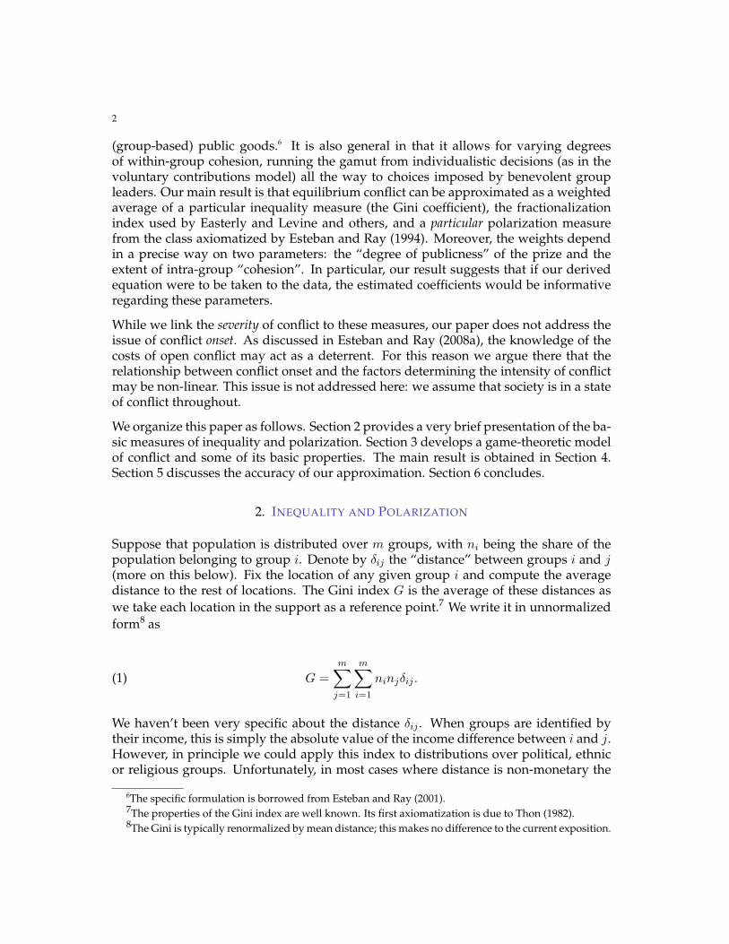
5.2.1. A Baseline Case. Our baseline exercise is the case of contests with quadratic costs.First consider large populations. Then, by the discussion in the previous section we maytake α = 0.5 without any loss of generality. We examine several degrees of publicnessin the payoffs: λ = 0, 0.2, 0.8 and 1.0 (we report on λ = 0.5 in a later variation). In eachof these cases, we take numerous random draws of a population distribution over fivegroups.

13

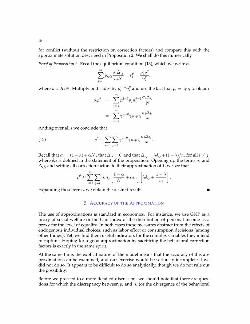
FIGURE 1. APPROXIMATE AND TRUE CONFLICT: BASELINE CASE

Figure 1 depicts the scatter plot of the approximate and true values of ρθ (ρ2, in this case).In each situation (and in all successive figures as well), we plot the true value of conflicton the horizontal axis and the approximation on the vertical axis. We also use the sameunits for both values, so that the diagonal, shown in every figure, is interpretable asequality in the two values. The top two panels perform simulations when private goodsare dominant (λ = 0.0, 0.2) and the bottom panels do the same when public goods aredominant (λ = 0.8, 1.0).

Remarkably, we obtain a very strong correlation between true and approximate valuesfor equilibrium conflict suggesting that the “behavior correction factors” do not play acritical role in explaining conflict.

Notice how we underapproximate the true value of conflict when λ is close to zero,and the overall conflict is small. This is related to the Pareto-Olson argument discussed

14

in the previous section. Low conflict will occur in non-polarized societies with one ormore small groups. When the conflict is over private goods (which is the case with λsmall), small groups will put in more resources per-capita. Because our approximationignores this effect, it underestimates conflict, especially when the value of that conflictis relatively small. In a similar vein, we tend to overestimate conflict (for small val-ues of conflict) when λ is close to 1. With public goods at stake, small groups put inless resources compared to their population share, and true conflict is smaller than theapproximation predicts.

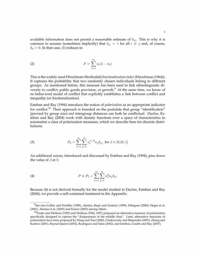
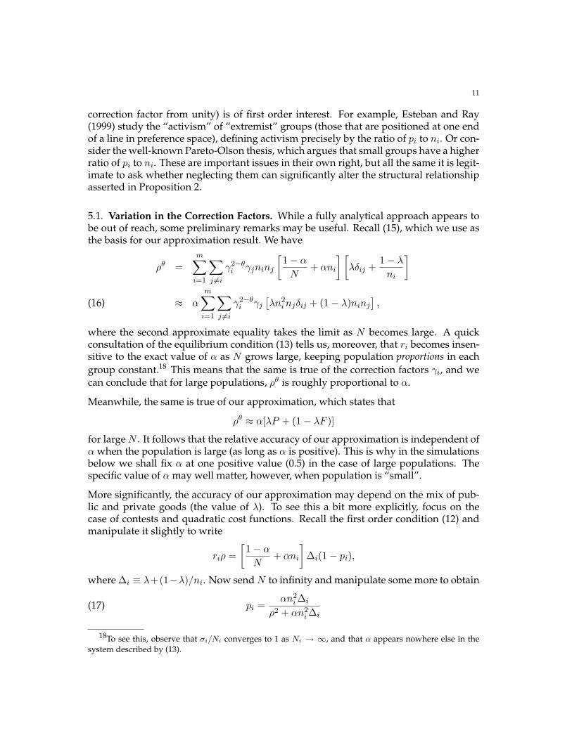
FIGURE 2. APPROXIMATE AND TRUE CONFLICT: VARYING UTILITY DISTANCES

That said, the correlation between the two variables is unaffected and the relationshipappears broadly linear. What is remarkable is how close the approximation really is,and yet how difficult it appears to be to get a handle on this analytically. That there isno simple relationship between the two values is evident from the highly nontrivial (yetconcentrated) scatter generated by the model.

15

However, note that in all situations, symmetric or near-symmetric population distribu-tions over all groups with positive populations will have the property that correctionfactors are unimportant. This is why there are regions in every panel where the simula-tions take us precisely to the diagonal.

This high correlation is retained in all the reasonable variations that we have studied.Some examples follow.

5.2.2. Inter-Group Distances. The next set of simulations studies varying inter-group dis-tances, instead of pure contests. Recall that distances are to be interpreted as losses fromhaving the other public goods in place, instead of the group’s favorite. We modify theprevious simulation and now permit utility losses to vary across groups pairs (retainingthe symmetry restriction that uij = uji). This is done by taking numerous independentdraws of the matrix describing pairwise utility losses. We retain the baseline specifica-tion in all other ways. The results are reported in Figure 2, for various values of λ. As inthe baseline case, the top panels perform simulations with private goods (λ = 0.0, 0.2)and the bottom panels do the same for public goods (λ = 0.8, 1.0). The correlations con-tinue to be remarkably high and the general features of the baseline case are retained.

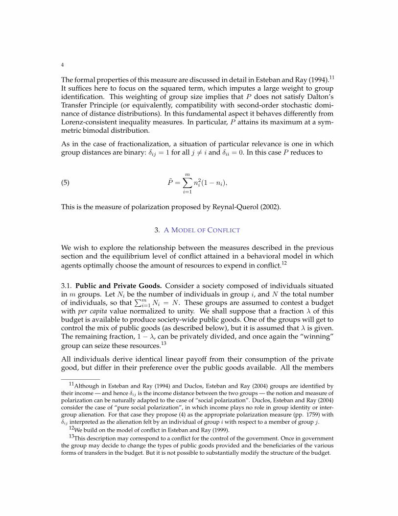
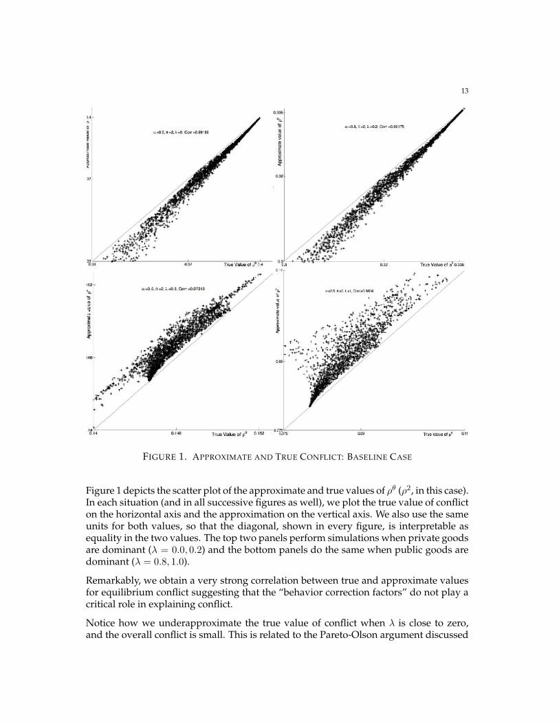
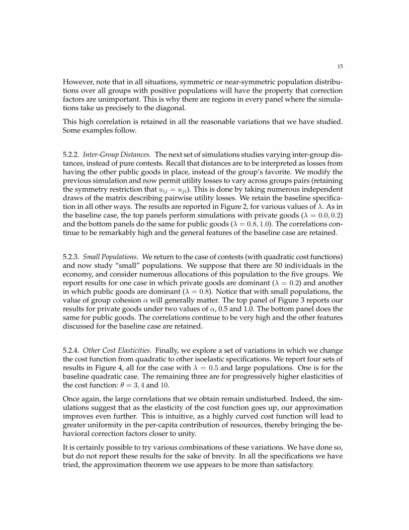
5.2.3. Small Populations. We return to the case of contests (with quadratic cost functions)and now study “small” populations. We suppose that there are 50 individuals in theeconomy, and consider numerous allocations of this population to the five groups. Wereport results for one case in which private goods are dominant (λ = 0.2) and anotherin which public goods are dominant (λ = 0.8). Notice that with small populations, thevalue of group cohesion α will generally matter. The top panel of Figure 3 reports ourresults for private goods under two values of α, 0.5 and 1.0. The bottom panel does thesame for public goods. The correlations continue to be very high and the other featuresdiscussed for the baseline case are retained.

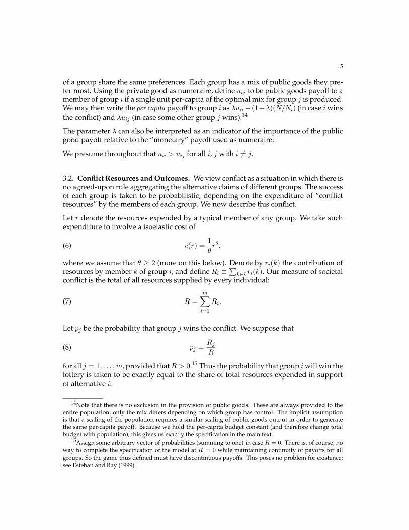
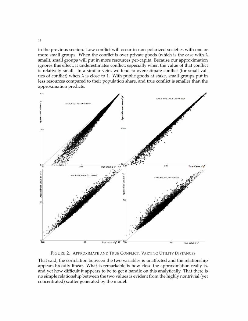
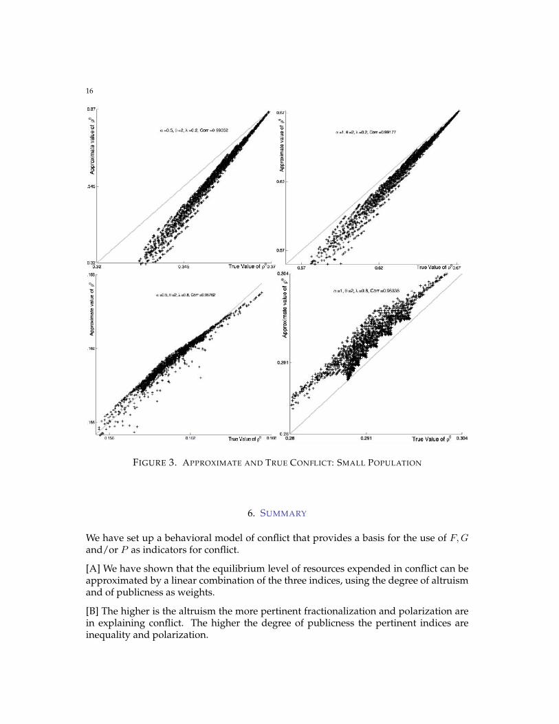
5.2.4. Other Cost Elasticities. Finally, we explore a set of variations in which we changethe cost function from quadratic to other isoelastic specifications. We report four sets ofresults in Figure 4, all for the case with λ = 0.5 and large populations. One is for thebaseline quadratic case. The remaining three are for progressively higher elasticities ofthe cost function: θ = 3, 4 and 10.

Once again, the large correlations that we obtain remain undisturbed. Indeed, the sim-ulations suggest that as the elasticity of the cost function goes up, our approximationimproves even further. This is intuitive, as a highly curved cost function will lead togreater uniformity in the per-capita contribution of resources, thereby bringing the be-havioral correction factors closer to unity.

It is certainly possible to try various combinations of these variations. We have done so,but do not report these results for the sake of brevity. In all the specifications we havetried, the approximation theorem we use appears to be more than satisfactory.

16

FIGURE 3. APPROXIMATE AND TRUE CONFLICT: SMALL POPULATION

6. SUMMARY

We have set up a behavioral model of conflict that provides a basis for the use of F,Gand/or P as indicators for conflict.

[A] We have shown that the equilibrium level of resources expended in conflict can beapproximated by a linear combination of the three indices, using the degree of altruismand of publicness as weights.

[B] The higher is the altruism the more pertinent fractionalization and polarization arein explaining conflict. The higher the degree of publicness the pertinent indices areinequality and polarization.

17

FIGURE 4. APPROXIMATE AND TRUE CONFLICT: NONQUADRATIC COSTS

[C] In simulations we find a very high correlation between our approximation and thetrue value of per capita conflict. This suggests that the behavior correction factors donot play a critical role.

Most importantly, this paper suggests new key features in explaining conflict: the de-gree of publicness in the payoff and the level of group mindedness in individual behav-ior. It seems plausible that the two dimensions are not independent of each other. Onewould expect high individualism in conflicts with a purely private payoff and highergroup motivation when the payoff sought is essentially public in nature. The connectionbetween these two dimensions is a matter of future research.

REFERENCES

BARRO, R.J. AND G.S. BECKER(1989) “Fertility Choice in a Model of Economic Growth,”Econometrica 57, 481-501.

18

BROCKETT, C.D. (1992) “Measuring Political Violence and Land Inequality in Central Amer-ica” American Political Science Review 86 (1992), 169-176.

CHAKRAVARTY, S.R. AND A. MAJUMDER(2001), “Inequality, Polarization and Welfare: The-ory and Applications,” Australian Economic Papers 40, 1–13.

COLLIER, P. AND A. HOEFFLER (2004), ”Greed and Grievance in Civil War” Oxford EconomicsPapers 56, 563-595.

DUCLOS, J-Y., J. ESTEBAN, AND D. RAY (2004), “Polarization: Concepts, Measurement,Estimation” Econometrica 72, 1737–1772.

EASTERLY W. AND R. LEVINE (1997), Africas Growth Tragedy: Policies and Ethnic Divisions,Quarterly Journal of Economics 111, 1203-1250.

ESTEBAN, J., C. GRADIN AND D. RAY (2007) An Extension of a Measure of Polarization, withan application to the income distribution of five OECD countries, Journal of Economic Inequality5, 1-19.

ESTEBAN, J. AND D. RAY (1994), “On the Measurement of Polarization” Econometrica 62, 819-852.

ESTEBAN, J. AND D. RAY (1999), “Conflict and Distribution” Journal of Economic Theory 87, 379-415.

ESTEBAN,J. AND D. RAY (2007), “A Model of Ethnic Conflict,” mimeo., Department of Econom-ics, new York University.

ESTEBAN, J. AND D. RAY (2008a), “Polarization, Fractionalization and Conflict,” Journal of PeaceResearch 45, 163-182.

ESTEBAN, J. AND D. RAY (2008b), “On the Salience of Ethnic Conflict,” American Economic Review98 forthcoming.

ESTEBAN, J. AND G. SCHNEIDER(2008) Polarization and Conflict: Theoretical and EmpiricalIssues (Introduction to the special issue), Journal of Peace Research 45, 131-141.

FEARON, J. AND D. LAITIN (2003), “Ethnicity, Insurgency, and Civil War,” American PoliticalScience Review 97, 75–90.

FOSTER, J. AND M.C. WOLFSON(1992), ”Polarization and the Decline of the Middle Class:Canada and the US”, Venderbilt University, mimeo.

LICHBACH, M. I. (1989), “An Evaluation of ”Does Economic Inequality Breed Political Con-flict?” Studies, World Politics 4, 431470.

MIDLARSKI, M.I. (1988), “Rulers and the ruled: patterned inequality and the onset of masspolitical violence,” American Political Science Review 82, 491–509.

MIGUEL, E., SATYANATH, S. AND E. SERGENTI (2004), “Economic Shocks and Civil Conflict:An Instrumental Variables Approach,” Journal of Political Economy 112, 725–753.

MONTALVO, J. G. AND M. REYNAL-QUEROL (2005a), “Ethnic Polarization, Potential Conflictand Civil War,” American Economic Review 95, 796–816.

19

MONTALVO, J. G. AND M. REYNAL-QUEROL(2005b) “Ethnic diversity and economic develop-ment” Journal of Development Economics 76, 293-323.

MULLER,E.N. AND M.A. SELIGSON (19987) “Inequality and Insurgency”, American Political Sci-ence Review 81, 425-451.

MULLER, E. N., M.A. SELIGSON AND H. FU (1989), “Land inequality and political violence”,American Political Science Review 83, 577–586.

NAGEL, J. (1974), “Inequality and discontent: a non-linear hypothesis,” World Politics 26, 453–472.

PANDE, R. AND D. RAY (2003), “Preliminary Notes on Inequality and Conflict,” mimeo.

REYNAL-QUEROL, M. (2002), ”Ethnicity, Political Systems, and Civil Wars” Journal of ConflictResolution 46, 29-54.

RODRIGUEZ, J.G. AND R. SALAS(2002), “Extended Bi-Polarization and Inequality Measures,”Research on Economic Inequality 9 69-84.

SAMBANIS, N. (2001), ”Do Ethnic and Non-Ethnic Civil Wars Have the Same Causes? A Theo-retical and Empirical Enquiry (Part 1)” Journal of Conflict Resolution 45, 259-282.

SEN, A.(1966) “Sen A. (1966), “Labour Allocation in a Cooperative Enterprise” Review of Eco-nomic Studies 33, 361-371.

SKAPERDAS, S. (1996), “Contest Success Functions,” Economic Theory 7, 283-290.

THON D.(1982) ”An axiomatization of the Gini coefficient”, Mathematical Social Science 2 131-143.

WANG, Y.Q. AND K.Y. TSUI(2000), “Polarization Orderings and New Classes of PolarizationIndices,” Journal of Public Economic Theory 2, 349–363.

WOLFSON, M. C. (1994), “When Inequalities Diverge”, American Economic Review Papers andProceedings 84 353-358.

WOLFSON, M.C.(1997), ”Divergent Inequalities: theory and empirical results”, Review of Incomeand Wealth 43 401-421.

ZHANG, X. AND R. KANBUR(2001), “What Difference Do Polarisation Measures Make? AnApplication to China,” Journal of Development Studies 37, 85–98.

APPENDIX

Esteban and Ray (1994) and Duclos, Esteban and Ray (2003) axiomatize the following class ofpolarization measures. Let population be distributed on [0,∞) with density f(x). The class isgiven by

Pβ = K

∫ ∫f(x)1+βf(y)|x− y|dxdy, for some constant K > 0 and β ∈ [0.25, 1].

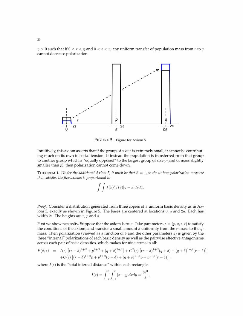
Axiom 5. Suppose that a distribution consists of three equi-spaced uniform basic densities ofsizes r, p and q, as shown in Figure 5, each of support 2ε. Assume that p = q + r. Then there is

20

η > 0 such that if 0 < r < η and 0 < ε < η, any uniform transfer of population mass from r to qcannot decrease polarization.

r p q

0 a 2a2! 2! 2!

FIGURE 5. Figure for Axiom 5.

Intuitively, this axiom asserts that if the group of size r is extremely small, it cannot be contribut-ing much on its own to social tension. If instead the population is transferred from that groupto another group which is “equally opposed” to the largest group of size p (and of mass slightlysmaller than p), then polarization cannot come down.

THEOREM 1. Under the additional Axiom 5, it must be that β = 1, so the unique polarization measurethat satisfies the five axioms is proportional to∫ ∫

f(x)2f(y)|y − x|dydx.

Proof. Consider a distribution generated from three copies of a uniform basic density as in Ax-iom 5, exactly as shown in Figure 5. The bases are centered at locations 0, a and 2a. Each haswidth 2ε. The heights are r, p and q.

First we show necessity. Suppose that the axiom is true. Take parameters z ≡ (p, q, r, ε) to satisfythe conditions of the axiom, and transfer a small amount δ uniformly from the r-mass to the q-mass. Then polarization (viewed as a function of δ and the other parameters z) is given by thethree “internal” polarizations of each basic density as well as the pairwise effective antagonismsacross each pair of basic densities, which makes for nine terms in all:

P (δ, z) = I(ε)[(r − δ)2+β + p2+β + (q + δ)2+β

]+ C2(ε)

[(r − δ)1+β(q + δ) + (q + δ)1+β(r − δ)

]+C(ε)

[(r − δ)1+βp+ p1+β(q + δ) + (q + δ)1+βp+ p1+β(r − δ)

],

where I(ε) is the “total internal distance” within each rectangle:

I(ε) ≡∫ ε

−ε

∫ ε

−ε|x− y|dxdy =

8ε3

3,

21

C(ε) is the “total distance” across neighboring rectangles:

C(ε) ≡∫ ε

−ε

∫ a+ε

a−ε(x− y)dxdy = 4aε2,

and C2(ε) is the “total distance” between the side rectangles:

C2(ε) ≡∫ ε

−ε

∫ 2a+ε

2a−ε(x− y)dxdy = 8aε2.

Differentiating P (δ, z) with respect to δ (write this partial derivative as P ′(δ, z)) and evaluatingthe result at δ = 0, we see that

P ′(0, z) = (2 + β)I(ε)[q1+β − r1+β

]+ (1 + β)C(ε)

[qβp− rβp

]− C2(ε)

[q1+β − r1+β + (1 + β)(rβq − qβr)

].

Substituting the values for I(ε), C(ε) and C2(ε), we see that14ε−2P ′(0, z) = (2 + β)

2ε3[q1+β − r1+β

]+ (1 + β)ap

[qβ − rβ

]− 2a

[q1+β − r1+β + (1 + β)(rβq − qβr)

].(19)

The axiom insists that P ′(0, z) must be nonnegative for all values of z such that p = q + r andr sufficiently small. Fixing p and a, take a sequence of z’s such that r → 0, q → p and ε → 0.Noting that P ′(0, z) ≥ 0 throughout this sequence, we can pass to the limit in (19) to concludethat

(1 + β)− 2 ≥ 0,which, given that β ≤ 1, proves that β = 1.

To establish the converse, put β = 1 and consider (19) again. We see that for any configurationwith q > r,

14ε−2P ′(0, z) = 2ε

[q2 − r2

]+ 2ap [q − r]− 2a

[q2 − r2

]> 2ap [q − r]− 2a(q − r)(q + r)= 2ap [q − r]− 2ap [q − r] = 0,

where the penultimate equality uses the restriction that p = q + r.