LINK STATE RELATIONSHIPS UNDER INCIDENT · PDF fileLINK STATE RELATIONSHIPS UNDER INCIDENT CONDITIONS: USING A CTM-BASED LINEAR PROGRAMMING DYNAMIC ... The effectiveness of these

LINK STATE RELATIONSHIPS UNDER INCIDENT CONDITIONS: USING A CTM-BASED LINEAR PROGRAMMING DYNAMIC TRAFFIC

ASSIGNMENT MODEL

FINAL REPORT

PennDOT/MAUTC Agreement Contract No. 510401 VT-2008-07

DTRS99-G-0003

Prepared for

Virginia Transportation Research Council

By

Weihao Yin Pamela Murray-Tuite

Virginia Polytechnic and State University March 2010

This work was sponsored by the Virginia Department of Transportation and the U.S. Department of Transportation, Federal Highway Administration. The contents of this report reflect the views of the authors, who are responsible for the facts and the accuracy of the data presented herein. The contents do not necessarily reflect the official views or policies of either the Federal Highway Administration, U.S. Department of Transportation, or the Commonwealth of Virginia at the time of publication. This report does not constitute a standard, specification, or regulation.

1. Report No.

2. Government Accession No. 3. Recipient’s Catalog No.

4. Title and Subtitle Link State Relationship under Incident Conditions: Using CTM-based Linear Programming Dynamic Traffic Assignment Model

5. Report Date March 2010 6. Performing Organization Code

7. Author(s) Weihao Yin and Pamela Murray-Tuite

8. Performing Organization Report No.

9. Performing Organization Name and Address Department of Civil and Environmental Engineering Virginia Polytechnic and State University Northern Virginia Center Falls Church, VA, 22043

10. Work Unit No. (TRAIS) 11. Contract or Grant No.

12. Sponsoring Agency Name and Address 13. Type of Report and Period Covered Final Report 8/10/2008– 8/10/2009 14. Sponsoring Agency Code

15. Supplementary Notes 16. Abstract Urban transportation networks, consisting of numerous links and nodes, experience traffic incidents such as accidents and road maintenance work. A typical consequence of incidents is congestion which results in long queues and causes high travel time variability. In order to combat the negative effects due to congestion, various mitigation strategies have been proposed and implemented in the United States and worldwide. The effectiveness of these congestion mitigation strategies for incident conditions largely depends on the accuracy of information regarding network conditions. Therefore, an efficient and accurate procedure to determine the link states, reflected by flows and density over time, is essential to incident management. This research project constructs a user equilibrium Dynamic Traffic Assignment (DTA) model using linear programming (LP) that incorporates the Cell Transmission Model (CTM) to evaluate the temporal variation of flow and density over links, which accurately reflect the link states of a transportation network. The proposed model adopts a scheme of bi-level optimization in which the upper level program determines the flows over the network while the lower level program (CTM) propagates flows according to widely-accepted traffic flow theory. Encapsulation of the CTM equips the model with the capability of accepting inputs of incidents like duration and capacity reduction. Moreover, the proposed bi-level model is capable of handling multiple origin-destination (OD) pairs, which is a strength that most LP-based DTA models do not possess. By using this model, the temporal variation of flows over links can be readily evaluated and thus it can be used to predict the time-dependent link states. The results of numerical examples show that the flow pattern preserves the user equilibrium principle and satisfies the First-In-First-Out (FIFO) condition. The link-based encapsulation of CTM is able to temporally capture the queue between links and fully mimics the spillback within links. The flow pattern resultant from the proposed LP-DTA procedure can be transformed to density variation diagrams of links. These visualized density predictions provide insights to link state relationships by graphically describing the states of all the links of a transportation network. The impact of incidents on links can be reflected by their density and flow variations during and after the incidents. The results of the numerical examples, by isolating the effects of the incident, show that the parallel routes of a specific OD pair display the relationship of substituting for each other, which is consistent with general expectations. A closer examination over the density variations confirms the existence of a substitution relationship between the unshared links of the two routes connecting an OD pair. Quantitative information about the additional traffic on the diversion route in terms of amount and duration of diverted traffic is also obtained. Two levels of application of link state relationships are identified for real-world situations. Information about link states for different incident scenarios can be aggregated and mined to derive general patterns for the link state relationships. These patterns can be used as general guidance for incident management purposes. A microscopic level of application involves usage of flow and density predictions for a specific incident to determine which specific incident management strategy (e.g. opening the HOV lane to all traffic or changing signal timing) is most beneficial. 17. Key Words Link states, Incident, Linear Programming, Dynamic Traffic Assignment

18. Distribution Statement No restrictions.

19. Security Classif. (of this report) Unclassified

20. Security Classif. (of this page) Unclassified

21. No. of Pages 40

22. Price

i

Abstract

Urban transportation networks, consisting of numerous links and nodes, experience traffic incidents such as accidents and road maintenance work. A typical consequence of incidents is congestion which results in long queues and causes high travel time variability. In order to combat the negative effects due to congestion, various mitigation strategies have been proposed and implemented in the United States and worldwide. The effectiveness of these congestion mitigation strategies for incident conditions largely depends on the accuracy of information regarding network conditions. Therefore, an efficient and accurate procedure to determine the link states, reflected by flows and density over time, is essential to incident management. This research project constructs a user equilibrium Dynamic Traffic Assignment (DTA) model using linear programming (LP) that incorporates the Cell Transmission Model (CTM) to evaluate the temporal variation of flow and density over links, which accurately reflect the link states of a transportation network. The proposed model adopts a scheme of bi-level optimization in which the upper level program determines the flows over the network while the lower level program (CTM) propagates flows according to widely-accepted traffic flow theory. Encapsulation of the CTM equips the model with the capability of accepting inputs of incidents like duration and capacity reduction. Moreover, the proposed bi-level model is capable of handling multiple origin-destination (OD) pairs, which is a strength that most LP-based DTA models do not possess. By using this model, the temporal variation of flows over links can be readily evaluated and thus it can be used to predict the time-dependent link states. The results of numerical examples show that the flow pattern preserves the user equilibrium principle and satisfies the First-In-First-Out (FIFO) condition. The link-based encapsulation of CTM is able to temporally capture the queue between links and fully mimics the spillback within links. The flow pattern resultant from the proposed LP-DTA procedure can be transformed to density variation diagrams of links. These visualized density predictions provide insights to link state relationships by graphically describing the states of all the links of a transportation network. The impact of incidents on links can be reflected by their density and flow variations during and after the incidents. The results of the numerical examples, by isolating the effects of the incident, show that the parallel routes of a specific OD pair display the relationship of substituting for each other, which is consistent with general expectations. A closer examination over the density variations confirms the existence of a substitution relationship between the unshared links of the two routes connecting an OD pair. Quantitative information about the additional traffic on the diversion route in terms of amount and duration of diverted traffic is also obtained.

ii

Two levels of application of link state relationships are identified for real-world situations. Information about link states for different incident scenarios can be aggregated and mined to derive general patterns for the link state relationships. These patterns can be used as general guidance for incident management purposes. A microscopic level of application involves usage of flow and density predictions for a specific incident to determine which specific incident management strategy (e.g. opening the HOV lane to all traffic or changing signal timing) is most beneficial.

iii

Table of Contents

Abstract ..................................................................................................................................... i

List of Figures .......................................................................................................................... v

List of Tables .......................................................................................................................... vi

Chapter 1 Introduction ..................................................................................................... 1

1.1. Methodology of the Study ..................................................................................... 1

1.1.1. Nature of Link States ...................................................................................... 1

1.1.2. Dynamic Traffic Assignment ........................................................................ 2

1.2. Objectives of the Study .......................................................................................... 2

1.3. Organization of the Report .................................................................................... 3

Chapter 2 Literature Review ........................................................................................... 4

2.1. Introduction ............................................................................................................. 4

2.2. Review of Analytical DTA models ....................................................................... 5

2.2.1. Mathematical programming formulations ................................................. 5

2.2.2. Optimal control formulations ....................................................................... 6

2.2.3. Variational inequality formulations ............................................................. 6

2.3. LP-DTA Models Based on the Cell Transmission Model ................................. 6

2.4. Summary .................................................................................................................. 8

Chapter 3 Model Formulation ......................................................................................... 9

3.1. Basic Assumptions ................................................................................................. 9

3.2. Upper Level Program .......................................................................................... 10

3.3. Lower Level Program .......................................................................................... 11

3.4. Properties of the Proposed Model ...................................................................... 15

3.5. Proof of Equivalence to DUE .............................................................................. 16

Chapter 4 Computational Experience of the Model .................................................. 19

4.1. Solving the Model ................................................................................................. 19

4.2. Numerical Examples ............................................................................................ 19

4.2.1. Single Origin Destination Pair .................................................................... 20

4.2.2. Multiple Origin Destination Pairs .............................................................. 23

4.3. Examination of Link State Relationships .......................................................... 27

iv

4.3.1. Multiple OD network ................................................................................... 27

4.4. Application of Link State Relationships ............................................................ 28

Chapter 5 Conclusions and Future Extensions ........................................................... 29

5.1. Conclusions ........................................................................................................... 29

5.2. Future Extensions ................................................................................................. 30

References .............................................................................................................................. 31

v

List of Figures

Figure 1 Time-Expanded Network .................................................................................... 10

Figure 2 Cell Partition within a Link ................................................................................. 11

Figure 3 Cumulative Counts of Vehicles of a Link ......................................................... 15

Figure 4 Flow Conservation between Time-space Links ................................................ 16

Figure 5 Solution Procedure ............................................................................................... 19

Figure 6 Two Test Networks ............................................................................................... 20

Figure 7 Density Variations of Links under the No-Incident Scenario ......................... 27

Figure 8 Density Variations of Links under the Incident Scenario (Severity = 0.6) .... 27

vi

List of Tables

Table 1 Summary of Notation ............................................................................................... 9

Table 2 Basic Characteristics of Single OD Pair Network ............................................... 20

Table 3 Demand Profile for Single OD Network ............................................................. 20

Table 4 Flow Pattern of Single OD Network (No Incident) ........................................... 21

Table 5 Flow Pattern Single OD Network (Incident Severity = 0.6) .............................. 22

Table 6 Flow Pattern of Single OD Network (Incident Severity = 1) ............................ 23

Table 7 Basic Characteristics of the Multiple OD Pairs Network .................................. 23

Table 8 Demand Profile for Multiple OD Pairs Network ............................................... 24

Table 9 Flow Pattern for Multiple OD Pairs Network (No Incident) ............................ 24

Table 10 Flow Pattern for Multiple OD Pair Network (Incident Severity = 0.6) ......... 25

Table 11 Flow Pattern for Multiple OD Pairs Network (Incident Severity =1) ........... 26

1

Chapter 1 Introduction

Urban transportation networks, consisting of numerous links and nodes, are vulnerable to various events ranging from natural disasters, such as hurricanes, to common traffic incidents, like accidents. A typical consequence of common incidents is congestion which results in long queues and causes high travel time variability. Congestion due to incidents constitutes at least 25% of total congestion (Cambridge Systematics, 2005). In addition, incidents account for approximately 60% of the vehicle hours lost to congestion (Robinson and Nowak, 1993). Congestion effects introduced by incidents are accentuated during peak hours. During peak hours when traffic flow approaches its capacity, the queue caused by lane closure possibly remains until the peak hours end (Helman, 2004). In order to combat the negative effects due to congestion, various mitigation strategies have been proposed and implemented in the United States and worldwide. Strategies commonly used include ramp metering as well as hard shoulder operation which aim to deal with recurrent congestion. For non-recurrent congestion mainly due to incidents, mitigation strategies adopted are variable speed limits, dynamic high-occupancy-vehicle (HOV) designations, and route diversion through variable message signs (Liu and Murray-Tuite, 2008). The effectiveness of implementing these strategies for incident conditions largely depends on the accuracy of information regarding network conditions. Particularly for the route diversion strategy, it is important to predict the amount of traffic diverted in order to ensure the effectiveness of the strategy; operations of the diverted routes may need to be adjusted accordingly to handle additional traffic due to the diversion. Therefore, an efficient and accurate procedure to determine the link states is essential to incident management. Moreover, understanding of the link state relationships can also be useful to provide general guidance for incident mitigation efforts. The remainder of this chapter is divided into three sections. The first section presents background to the study methodology by discussing the nature of link states and dynamic traffic assignment. The objectives of the study are presented in the second section and the last section presents the organization of the report.

1.1. Methodology of the Study

1.1.1. Nature of Link States

The states of the links that constitute a traffic network cannot be described exclusively by binary indicators for detailed analyses. Such dichotomous descriptions like “connected” and “disconnected” are suitable for utility networks because the connection status of links are of most interest under usual circumstances. However, under most occasions, links of a transportation network exhibit intermediate states rather than extreme states such as “disconnected.” Furthermore,

2

the link states are dynamic. Therefore, continuous measurements that have a time dimension are needed to accurately describe the link states of a traffic network. Fortunately, the traffic conditions on a specific link can be described using measures from well-established traffic theory such as flow, density and speed, which are dynamic and continuous. In addition to the difficulty of state description, the human factor adds to the complexity of determining the link states. Drivers tend to re-route when incidents occur especially when information about the traffic conditions is available. This is very different from communication networks in which signal traffic, under normal conditions, would not divert from the pre-determined route spontaneously. This is different from what people can do under similar conditions within a transportation network. In other words, the route choice of network traffic possesses a dynamic nature. Therefore, in order to predict the link states, this re-routing behavior needs to be captured. The existence of intermediate link states, combined with the dynamic nature of drivers’ route choice, leads to complicated link state relationships. Specifically, link state relationships may change over time and cannot be excessively synthesized into simple descriptions. Therefore, a complete evaluation of the dynamic variations of link states is necessary to facilitate the understanding of the link state relationships.

1.1.2. Dynamic Traffic Assignment

The static traffic assignment problem is defined as determining the flows for each link of a transportation network based on known demand (origin-destination matrix) and link performance functions (Sheffi, 1985). The Dynamic Traffic Assignment (DTA) departs from this definition by dealing with time-dependent flows. In addition, DTA is inherently characterized by the need to adequately represent traffic realism and human behaviors, which are, to some extent, reflected by the assignment principles like user-equilibrium (UE). The UE principle assumes that network users, or drivers, can choose their departure time and paths freely. Therefore, the output of a DTA procedure based on UE principle provides all the necessary elements to describe link states and subsequently understand link state relationships. User Equilibrium Dynamic Traffic Assignment (UE-DTA) is applied for this study since it gives both the required flow measurements and captures the re-routing behavior.

1.2. Objectives of the Study

The objectives of this study can be described as follows: In order to efficiently and accurately determine the link states, this research

project constructs a linear programming model that incorporates the Cell Transmission Model (CTM) based on Carey’s bi-level DTA framework (2009). The proposed model contributes to the existing literature by equipping the

3

model with the capability of modeling transient traffic as well as handling multiple OD pairs without first-in-first-out (FIFO) violation within the UE framework, which is a merit that most LP-based models do not possess. By using this model, the temporal variation of flows over links can be readily evaluated and thus it can predict the link states.

Transform the predicted flows into temporal density variations to evaluate link states of a traffic network. The temporal density variations are graphically presented thus facilitating interpretation.

1.3. Organization of the Report

The rest of the report is organized as follows. The next chapter reviews research efforts in the DTA field and focuses on various analytical formulations. Chapter 3 lays out the formulation of the model, discusses some properties of the proposed model and presents the proof of equivalence to dynamic user equilibrium. Numerical examples are provided in Chapter 4. Based on the results for the two sample networks, basic insights into link state relationships are provided in Chapter 5, as well as conclusions and future directions.

4

Chapter 2 Literature Review

Since dynamic traffic assignment is applied to identify the link state relationships, only literature relevant to DTA will be reviewed here. To the authors’ best knowledge, no alternative methods have been used to identify the link state relationships for a transportation network.

2.1. Introduction

DTA has received a lot of attention due to its significance in predicting traffic patterns within a transportation network for controlling and managing the network. According to different assignment principles, DTA problems fall into two general categories, namely, system optimum and user equilibrium. If the time-dependent origin-destination matrices are assumed to be known, in Dynamic User Equilibrium (DUE), users choose paths whose travel costs (time) are no higher than those on other available paths. If users are at the liberty of choosing departure times, the complete definition of DUE virtually implies users cannot shorten their travel time by unilaterally changing paths or departure time, which is similar to the definition of static user equilibrium presented in (Sheffi, 1985). The system optimum principle distinguishes itself from user equilibrium by requiring users to make route decisions for the sake of the network-wise benefit, or more specifically, minimization of the total travel costs of all the users. There are numerous research papers regarding the DTA problem. Solution methods for DTA can be synthesized into two major approaches: computer simulation and analytical models. Based on the mathematical techniques applied, analytical models can be classified into three categories: mathematical programming, optimal control theory, and variational inequality (Peeta and Ziliaskopoulos, 2001). Most analytical formulations, developed in the past two decades, tend to focus on user equilibrium (UE) and system optimum (SO), or variants of them such as incorporation of the stochastic nature of travel time. Review of simulation-based models is out of the scope of this project report. It should be noted that real-time deployment of DTA models and realistic operational performance are always among the objectives of any DTA models. Regardless of the mathematical techniques the analytical models apply, conflict always exists between tractability and modeling details, especially when traffic flow behaviors are considered within links of a traffic network. It is relatively difficult to incorporate traffic behaviors into mathematical programs or other analytical frameworks compared to discrete simulation. Aiming to overcome this difficulty, numerous research efforts, have been devoted to incorporating traffic flow models into DTA solving mechanisms. A quite natural idea is to absorb the traffic flow model into the network assignment procedure. Some models are hard to solve due to non-linearity of the travel time function or travel time calculation procedures they

5

adopt. These DTA formulations, incorporating various traffic flow models, will be discussed in the next section in greater detail. In addition to the requirement of realistic representation of traffic dynamics, it is important to model various external disruptions, such as traffic incidents, within the DTA modeling frameworks. With the availability of information about the incident occurrences, travelers have the option to change their routes along the way. This re-routing behavior, or diversion, may significantly influence the traffic pattern of a certain network especially within the DTA context. Hence, the capability of modeling transient incidents should be considered critical for DTA models.

2.2. Review of Analytical DTA models

2.2.1. Mathematical programming formulations

The applications of mathematical programming techniques to DTA were pioneered by Merchant and Nemhauser (1978a; 1978b). Their formulation (M-N model) deals with a simple deterministic problem of a fixed demand, single-destination network within the system optimum context. A typical problem within this SO formulation as well as many other SO models is First-In-First-Out (FIFO) violation. FIFO conditions make a lot of algorithms unsolvable analytically due to the fact that it invites non-convexity to mathematical programs (Peeta and Ziliaskopoulos, 2001). Compared to analytical models, FIFO compliance is not a problem for simulation models since it is easy to track each vehicle and thus maintain the FIFO condition. Another problem associated with some SO formulations like the M-N model relates to “holding-back” vehicles on links. In other words, certain traffic streams are intentionally favored over others to minimize the system delays (Carey and Subrahmanian, 2000). Studies by Janson (1991a; 1991b) are the first formulations attempting to model DTA under the UE principle. Non-linear mixed integer constraints were applied for the purpose of ensuring temporal continuity of OD flows. It is noted by other authors such as Peeta and Ziliaskopoulos (2001), that this model led to unrealistic traffic behaviors and relied on static link travel time functions. In order to realistically capture traffic behaviors, several authors attempted to accommodate traffic stream models into mathematical programming DTA models. Bi-level mathematical programs that encapsulate Greenshields’ traffic flow model (Jayakrishnan, Tsai et al. 1995; Jayakrishnan, Chen et al. 1999) represent those early attempts. As noted by Peeta and Ziliaskopoulos (2001), mathematical programming approaches have their limitations in strict adherence to dynamic optimality conditions and retaining the FIFO property as well as realistic traffic dynamics for general networks.

6

2.2.2. Optimal control formulations

In an optimal control modeling framework, both OD demands and traffic flows are considered as continuous functions of time, different from mathematical programming formulations. Friesz, Luque et al. (1989) proposed a link-based optimal control formulation for both SO and UE objectives for the single-destination case. The central assumption was continuous modifications to routing decisions based on changing network conditions. They also generalized Beckmann’s equivalent optimization problem for static UE traffic assignment as an optimal control problem, which lacks of efficient solution algorithm. By defining link inflows and outflows as control variables, Ran and Boyce (1994) transformed the DUE problem into a convex model using the Frank-Wolfe algorithm, which is easy to solve relative to the non-convex model. The limitations of optimal control formulations lie in their lack of explicit constraints to preclude FIFO violations and sound procedures to maintain traffic realism and more importantly a solution procedure for general networks (Peeta and Ziliaskopoulos, 2001).

2.2.3. Variational inequality formulations

The strengths of variational inequality (VI) derive from its unified mechanism to address equilibrium and equivalent optimization problems (Peeta and Ziliaskopoulos, 2001). Moreover it can handle more realistic traffic scenarios. The study by Dafermos (1980) serves as the pioneer to use the VI approach for the traffic equilibrium problem. The model presented in (Huey-Kuo and Che-Fu, 1998) demonstrated the feasibility of VI approach within the UE-DTA context by relating travel time of a link exclusively with link inflow. A more influential model (Lo and Szeto, 2002) developed a variational inequality model that uses CTM as the underlying traffic flow model. This model successfully meets the FIFO condition and more importantly, is capable of capturing traffic dynamics. It can mimic the queue accumulation and dissipation under capacity reduction scenarios, which is substantial progress for DTA models using the VI approach. This formulation successfully circumvented traffic realism issues that were raised towards the VI approach in (Peeta and Ziliaskopoulos, 2001) and essentially made it possible for the VI approach to achieve both computational tractability and traffic realism.

2.3. LP-DTA Models Based on the Cell Transmission Model

The Cell Transmission Model (Daganzo, 1994; Daganzo, 1995) provides a set of linear equations that are a numerical approximation of the Lighthill-Whitham-Roberts model (Lighthill and Whitham, 1955; Richards, 1956), or LWR model. Ever since its inception, the CTM received great attention from researchers who focus on dynamic

7

traffic assignment due to its mathematical simplicity for encapsulation in an analytical framework. Ziliaskopoulos (2000), in a pioneering work, applied the CTM to a dynamic traffic assignment problem. The single-destination system optimum dynamic traffic assignment problem was formulated as an LP model based on CTM. Since there was only one origin-destination pair and system optimum was in effect, FIFO did not pose a threat to the analytical formulation. Though the model does not have much operational value for actual applications (Peeta and Ziliaskopoulos, 2001), it did provide insights into the DTA problem by raising the concept of marginal travel time and more importantly, explored the possibility of linear formulation of DTA based on the CTM. Inspired by the aforementioned work, various extensions to the LP-DTA model have been made. The single-destination assumption was relaxed by Li and Ziliaskopoulos (1999). They designated fixed arrival windows for all vehicles of the network and set the objective function to minimize the total travel time experienced for all users within the network. While the two papers by Ziliaskopoulos and his colleagues formulated the system optimum DTA (SO-DTA) problems for single and multiple destinations, another significant contribution to the linear programming model for SO-DTA problem was made by Waller and Ziliaskopoulos (2006). It presented a stochastic extension to the Ziliaskopoulos’ deterministic LP model. The paper proposed a chance-constrained based formulation which provided a robust SO solution when the level of reliability is specified by users. Though Ziliaskopoulos and his colleagues did not propose analytical formulations for user-equilibrium DTA (UE-DTA), they developed heuristic algorithms for UE-DTA problems. Waller and Ziliaskopoulos (2006) developed a combinatorial algorithm for the single-destination UE-DTA problem based on CTM. The conceptual framework is straightforward. Vehicles are always assigned to the time-dependent shortest paths, which are calculated at the beginning of each iteration. Attempts were made to extend the algorithm to the multi-destination UE-DTA problem though vehicles were assumed to take fixed routes (Waller and Ziliaskopoulos, 2006). Similar work includes Golani and Waller (2004). It can be seen that LP DTA models proposed by Ziliaskopoulos and his colleagues are able to obtain robust solutions for the single-destination system optimum DTA problem. Under certain assumptions, the model can be extended to incorporate multiple origin-destination pairs. Unfortunately, their models are not capable of analytically dealing with the UE-DTA problem though heuristics for UE-DTA are developed. Aiming to tackle the UE-DTA problem within a linear programming framework, Carey and his colleagues proposed an LP framework for the single-destination UE-DTA problem. Essentially, Carey’s DTA framework (Carey and Subrahmanian, 2000; Carey 2009) is a bi-level mathematical program whose upper level program is

8

formulated as a system-optimum DTA problem and lower level program is referred to as the link sub-model. The link sub-model predicts traffic flow over each link at each time interval. These link flow predictions are then fed back to the upper level program and serve as link capacity at each time interval. By iterating between the upper and lower level program, a UE-DTA solution is obtained when convergence is reached.

2.4. Summary

Analytical dynamic traffic assignment models mainly apply three categories of mathematical techniques, namely mathematical programming, optimal control theory and variational inequality approach. It can be noted that a persistent issue is the need to balance between mathematical tractability and traffic realism. Reasons for this problem include difficulty in incorporating traffic flow models and non-convexity invited by the FIFO condition. Research efforts are still needed to overcome the aforementioned difficulties and realize large-scale applications at reasonable expenses. To distinguish itself from previous LP-based DTA models, the proposed model deals with multiple origin-destination pairs while Ziliaskopoulos (2000) focused on the single-destination case within the SO context. Extending the works by Carey (2009) and Cary and Subrahmanian (2000), the proposed model is capable of modeling incidents under the UE-DTA framework.

9

Chapter 3 Model Formulation

The model presented here is an extension of the linear programming dynamic traffic assignment (LP-DTA) framework proposed by Carey (2009). The following notation is used throughout the report.

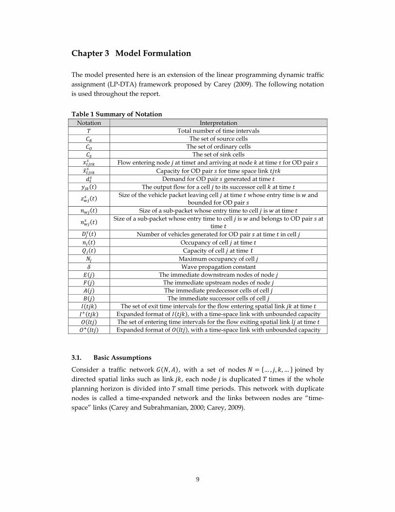
Table 1 Summary of Notation Notation Interpretation

Total number of time intervals The set of source cells The set of ordinary cells The set of sink cells

Flow entering node at time and arriving at node at time for OD pair Capacity for OD pair for time space link

Demand for OD pair generated at time The output flow for a cell to its successor cell at time

Size of the vehicle packet leaving cell at time whose entry time is and bounded for OD pair

Size of a sub-packet whose entry time to cell is at time

Size of a sub-packet whose entry time to cell is and belongs to OD pair at time

Number of vehicles generated for OD pair at time in cell Occupancy of cell at time Capacity of cell at time t

Maximum occupancy of cell Wave propagation constant

The immediate downstream nodes of node The immediate upstream nodes of node The immediate predecessor cells of cell The immediate successor cells of cell The set of exit time intervals for the flow entering spatial link at time Expanded format of , with a time-space link with unbounded capacity The set of entering time intervals for the flow exiting spatial link at time Expanded format of , with a time-space link with unbounded capacity

3.1. Basic Assumptions

Consider a traffic network , , with a set of nodes … , , , … joined by directed spatial links such as link , each node is duplicated times if the whole planning horizon is divided into small time periods. This network with duplicate nodes is called a time-expanded network and the links between nodes are “time-space” links (Carey and Subrahmanian, 2000; Carey, 2009).

10

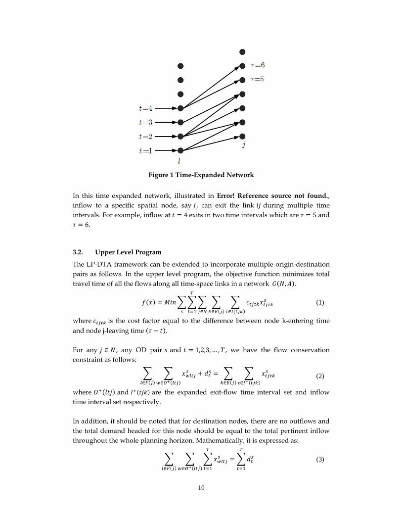
Figure 1 Time-Expanded Network

In this time expanded network, illustrated in Error! Reference source not found., inflow to a specific spatial node, say , can exit the link during multiple time intervals. For example, inflow at 4 exits in two time intervals which are 5 and

6.

3.2. Upper Level Program

The LP-DTA framework can be extended to incorporate multiple origin-destination pairs as follows. In the upper level program, the objective function minimizes total travel time of all the flows along all time-space links in a network , .

∈∈∈

(1)

where is the cost factor equal to the difference between node k-entering time and node j-leaving time . For any ∈ , any OD pair and 1,2,3, … , , we have the flow conservation constraint as follows:

∈∈ ∈∈

(2)

where and are the expanded exit-flow time interval set and inflow time interval set respectively. In addition, it should be noted that for destination nodes, there are no outflows and the total demand headed for this node should be equal to the total pertinent inflow throughout the whole planning horizon. Mathematically, it is expressed as:

∈∈

(3)

11

where is the destination node of OD pair . The capacity constraint confines the maximum flows along each time-space link, which is expressed by the equation:

, ∈ (4)

Note that flow conservation constraints (eq. (2) and eq. (3)) use expanded format of the set of link exit time intervals. The reasons are discussed as follows. Essentially, the capacity constraint (eq. (4)) excessively confines the flows over time-space links by not allowing more flows from upstream links to enter the current link, which could lead to infeasibility of the whole program. Hence, an additional unbounded time-space link is introduced. For example, if the time-space link with highest cost is link tjτk , then this extra time-space link is 1 with unbounded capacity. Introduction of this unbounded time-space link expands the exit time set to

. This extra time-space link ensures users’ free choice of spatial paths (Carey 2009). All the flows should be non-negative, which is expressed by:

0, ∀ , , ∈ , (5)

Objective function of eq.(1), together with the flow conservation constraints (eq.0, (3)), capacity constraint (eq.(4)) and non-negativity constraint (eq.(5)) completes the upper level program.

3.3. Lower Level Program

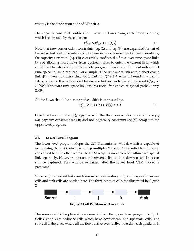
The lower level program adopts the Cell Transmission Model, which is capable of maintaining the FIFO principle among multiple OD pairs. Only individual links are considered here. In other words, the CTM recipe is implemented within each spatial link separately. However, interaction between a link and its downstream links can still be captured. This will be explained after the lower level CTM model is presented. Since only individual links are taken into consideration, only ordinary cells, source cells and sink cells are needed here. The three types of cells are illustrated by Figure 2.

Figure 2 Cell Partition within a Link

The source cell is the place where demand from the upper level program is input. Cells , and are ordinary cells which have downstream and upstream cells. The sink cell is the place where all the flows arrive eventually. Note that each spatial link

12

has its own dummy source cell and sink cell. In addition, vehicles arriving at the sink cell of a specific link do not necessarily successfully enter the source cell of a downstream link. The vehicles in the sink cell of an upstream link advance to the source cell of the downstream link depending on space availability, consistent with the FIFO rule. This procedure propagates multi-OD traffic based on the CTM recipe while maintaining the FIFO condition. The procedure can be conceptually described as follows. Each vehicle packet is made up of several sub-packets which are distinguished by entry time interval and OD pair. At each time interval throughout the whole planning horizon, the sub-packets that can leave are determined based on their respective entry time interval. In order to maintain FIFO, the sub-packet that enters earlier should always leave earlier compared to those entering later. The specifics are illustrated in the coming paragraphs. The planning horizon starts from time interval 1 and it is assumed that initial conditions of all the cells are known. Specifically, we set all the occupancies and flows equal to zero at the very beginning. The connection between the upper level program and lower level CTM model is the capacity of each time-space link . Note that the capacity constraint is not applicable to the additional unbounded time-space link aforementioned. Therefore, the exit time interval belongs to the set . After the solution to the upper level program is obtained, the flow variables are summed up by using the following equation:

∈

(6)

where signifies the total flow of OD pair entering the spatial link at time t . This total flow will be input into the lower level model as demand generated in the dummy source cell for the spatial link . In other words, eq.(4) and (6) are the connection between the upper level and lower level program. The first step of the lower level program finds the aggregate flow according to the CTM flow propagation equations (Daganzo, 1995) which are presented as follows. At any time , the output flow for cell to its successor cell can be calculated by the following equation:

, , , , ∈ (7)

It can be seen that the outflow is determined by cell capacities, denoted by and , current occupancy and the shockwave effect represented by the term

. With the outflow, the cell occupancies can be updated by using eq.(8) as follows.

1 , ∈ , ∈ (8)

Note that if cell is a source cell there is no inflow to it, or equivalently 0, ∀ , ∈ . If cell is a sink cell then no demand would be generated in this cell

13

and there is no output flow at any time. In other words, two conditions 0 and 0 hold at any time . Ordinary cells can have inflow and outflow but no demand. Hence, eq.(8) can be used to update cell occupancy for any category of cell at any time. In order to determine which sub-packets can leave at a specific time period, it is necessary to identify the sub-packets that are present in the current time interval. It has to be noted that the size of some vehicle sub-packets may be zero since it is possible that no vehicles enter this cell at a certain time. For cell at time interval , the sub-packets may enter this cell at any time interval prior to or at time interval . If the number of different OD pairs is , then totally the maximum number of sub-packets within a cell at any time is . For example, at 2, the maximum number of sub-packets within cell is 4 if there are two OD-pairs. Since sub-packets with early entry time should always leave earlier regardless of their destinations, it is essential to know occupancy disaggregated only by entry time interval at time , which is computed by:

(9)

There should always exist an entry time interval such that for any time interval ,

, , ∈ (10)

In eq. (10), is the outflow for cell to its successor cell at time , which is known from eq. (7). Eq. (10) essentially indicates that the packets with an arrival time interval earlier than should advance to the downstream cell in their entirety while the ones arriving later than this specific time interval should be split. In addition, we can always identify the packets leaving as a whole for OD pair by the summation ∑ . The FIFO principle requires that vehicle sub-packets that enter before and at should leave while only part of the sub-packet can leave. Since we have

multi-OD flows, we need to determine the proportions of this sub-packet allocated to each OD pair. We use the procedures presented in (Ge and Carey, 2004) to determine these proportions. The remaining part in the outflow packet after excluding packets leaving in their entirety is calculated as:

, ∈ (11)

In eq. (11), ∑ calculates the packets leaving in their entirety after the interval has been determined by eq.(10). The outflow allocated to each OD-pair is proportional to the size of the sub-packet of this OD-pair. The mathematical expression takes the form:

14

, ∀ (12)

By using eq. (9) to (12), we can determine the output flow disaggregated only by OD-pair,

, ∀ , ∈ (13)

So far we have determined the packets that can leave cell at time interval ; additional manipulations are needed to update the vehicle packet lists for the cells and their downstream cells. More specifically, we can calculate outflow disaggregated by both entry time interval and OD-pair as follows. For notational clarity purposes, a single variable is introduced to denote the flow for OD pair leaving cell at time whose entry time is . It can be used to update the packet list

for each cell.

,

, 1

0, 1

(14)

Eq. (14) essentially summarizes the flow calculation results presented in eq. (9) to eq. (13).

If the entry time of a packet is earlier than (determined in eq. (10)), it is supposed to leave the current cell in its entirety. Hence, we have .

If the entry time of a packet is equal to 1, this packet cannot leave as a whole. Only part of it can leave cell . Thus we have and

If the entry time of a packet is later than 1, it will not leave cell . In order to continue to track disaggregated flows and occupancy, we need to update the occupancy for the next time step. Flows leave cell so we have:

1 (15)

The output flow leaving at time from cell arrives at cell after one time interval. As a result, we have:

1 , ∀ , ∉ , ∈ (16)

In addition, if we consider the external demand as inflow to the source cell, in a similar fashion to eq.(16), we have:

1 , ∈ , ∀ (17)

Using eq. (15), (16) and (17), we calculate the disaggregated occupancies for the next time period. Cell FIFO ensures path FIFO as well as OD FIFO, which is proved in (Lo and Szeto, 2002). Hence, the cumulative arrival disaggregated by OD-pair in the sink cell can be used to determine the travel time for the whole link. The procedures used are explained with a concrete example.

15

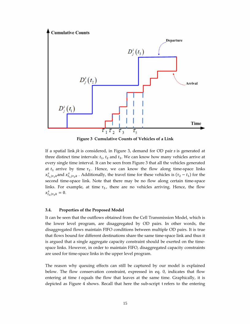
Figure 3 Cumulative Counts of Vehicles of a Link

If a spatial link is considered, in Figure 3, demand for OD pair is generated at three distinct time intervals: , and . We can know how many vehicles arrive at every single time interval. It can be seen from Figure 3 that all the vehicles generated at arrive by time . Hence, we can know the flow along time-space links

and . Additionally, the travel time for these vehicles is for the second time-space link. Note that there may be no flow along certain time-space links. For example, at time , there are no vehicles arriving. Hence, the flow

0.

3.4. Properties of the Proposed Model

It can be seen that the outflows obtained from the Cell Transmission Model, which is the lower level program, are disaggregated by OD pairs. In other words, the disaggregated flows maintain FIFO conditions between multiple OD pairs. It is true that flows bound for different destinations share the same time-space link and thus it is argued that a single aggregate capacity constraint should be exerted on the time-space links. However, in order to maintain FIFO, disaggregated capacity constraints are used for time-space links in the upper level program. The reason why queuing effects can still be captured by our model is explained below. The flow conservation constraint, expressed in eq. 0, indicates that flow entering at time equals the flow that leaves at the same time. Graphically, it is depicted as Figure 4 shows. Recall that here the sub-script t refers to the entering

16

time of the flow packet. The inflow to spatial node at time interval equals the outflow from the node in two time intervals.

Figure 4 Flow Conservation between Time-space Links

As mentioned in the previous section, each link is associated with a dummy source cell and sink cell. The inflow to a specific time-expanded node, say , is treated as demand generated at time in the dummy source cell. Due to flow conservation, this inflow is effectively equal to the outflow at time-expanded node . Moreover, this “dummy demand” is loaded in a strict chronological order from the beginning of the modeling horizon to the end. Hence, even if all the flows can move into the sink cells, this does not necessarily mean that they have entered the downstream link, which may not have adequate available space for additional incoming flows. Recall that each link has its own sink cell and source cell and the sink cell of a link is not the source cell of its downstream link. Therefore, entering the sink cell means the flows have left the link that contains this sink cell however it does not necessarily mean that these flows have entered the downstream link. Since demand is loaded sequentially, it is possible that the first cell of the downstream link cannot receive a vehicle packet at a certain time . Vehicles have to wait for a certain period of time. In this way, this model is able to capture the temporal effect of spillback. The inflow at time may not advance immediately due to congestion in downstream cells. As a result, the temporal effect of spillback, which is longer waiting time is captured between links. It should be noted that within each link, the spillback effects can be fully captured by the CTM recipe.

3.5. Proof of Equivalence to DUE

According to Carey (1999), three categories of paths can be identified: i. Fully utilized paths are paths on which one or more links constituting the path

carry flow to full capacity.

17

ii. Partially utilized paths are paths on which every link carries flow, but no links have flow to their full capacity.

iii. Available unutilized paths are paths on which there is at least one link carrying no flow while other links carry flow under the capacity limit.

The definition for dynamic user equilibrium in a time-expanded network is as follows (Carey 1999): DUE Definition: Links have fixed capacities. A traffic assignment is a UE if for each OD pair, FIFO is satisfied and the trip time on all partially utilized paths is not higher than the trip time on any available unutilized path, and is not lower than the trip time on any fully utilized path. The upper level program is constituted by eqs. (1) -(4). For notational simplicity, eq.0 can be rewritten as:

∈∈ ∈∈

, (18)

and are non-negative dual variables associated with their respective constraints and corresponds to the capacity constraint (eq.(4)). The proof uses Kuhn-Tucker optimality conditions which are necessary and sufficient for a linear program since a linear program is always a convex optimization problem (Bertsekas, 1999). For a specific OD pair , the Lagrangian of the linear program can be formulated as follows. Note that the OD-pair super-script is dropped for simplicity.

, , (19)

At the stationary point of the Lagrangian *x ,we have

, ,

and, ,

0 (20)

With respect to the dual variables, the following conditions have to hold:

, ,

and, ,

0 (21)

All the conditions expressed in eq.(20) and (21) can be written in the expanded form as:

0

0

0

(22)

where is the cost factor equal to . In addition to eq. (22), we have:

0

0

(23)

18

Eq. (22) and (23), together with flow conservation in eq. (18) are KT conditions for the linear program. By definition, the actual path travel time (p. t. t) is the summation of travel times of all the links traversed along the path irrespective of the path category. Mathematically,

. .

∈

(24)

where denotes the path connecting node to the destination node at time . From eq.(22), we know:

(25)

We can write an equation similar to eq. (25) for each time-space node along the path . By adding these equations, we have:

∈∈ ∈

(26)

If path is an available unutilized path, then flows on all the links are

below capacity. As a result, by the complementary slackness condition in eq.(23) we know all the dual variable are equal to zero. Hence, eq. (26) becomes:

∈∈

. . (27)

Note that right-hand side of eq. (27) is the actual path travel time expressed in eq. (24).

If path is a fully utilized path, then flows on all the links are greater than zero. So by complementary slackness in eq. (22), eq. (26) hold as a strict equality as follows:

∈∈ ∈

. . (28)

If path tjp is a partially utilized path, then all the flows are below capacity but

greater than zero. Hence we have:

∈∈

. . (29)

From eq. (27), (28) and (29) , we can know that at any time t , travel time along a partially utilized path is not higher than the trip time on any available unutilized path, and is not lower than the trip time on any fully utilized path. This is consistent with the dynamic user equilibrium definition presented at the beginning of this section.

19

Chapter 4 Computational Experience of the Model

4.1. Solving the Model

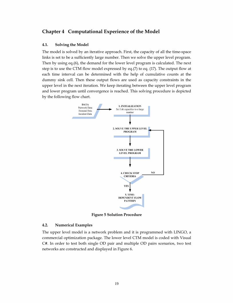
The model is solved by an iterative approach. First, the capacity of all the time-space links is set to be a sufficiently large number. Then we solve the upper level program. Then by using eq.(6), the demand for the lower level program is calculated. The next step is to use the CTM flow model expressed by eq.(7) to eq. (17). The output flow at each time interval can be determined with the help of cumulative counts at the dummy sink cell. Then these output flows are used as capacity constraints in the upper level in the next iteration. We keep iterating between the upper level program and lower program until convergence is reached. This solving procedure is depicted by the following flow chart.

Figure 5 Solution Procedure

4.2. Numerical Examples

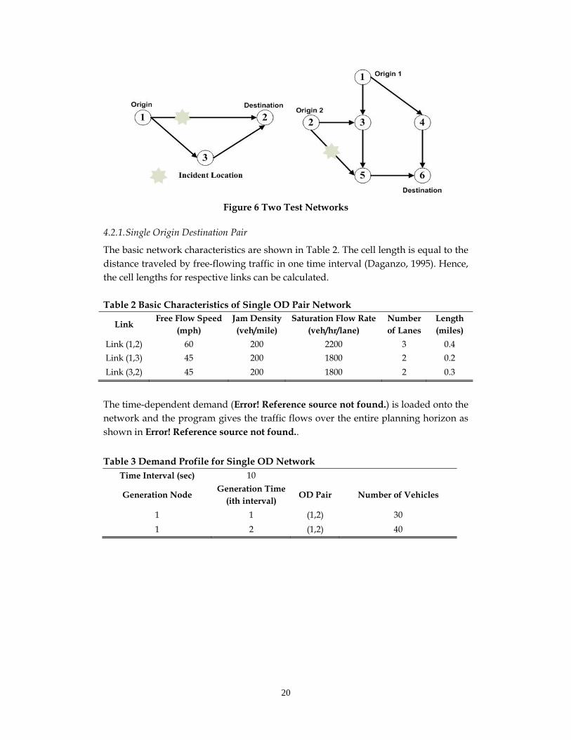
The upper level model is a network problem and it is programmed with LINGO, a commercial optimization package. The lower level CTM model is coded with Visual C#. In order to test both single OD pair and multiple OD pairs scenarios, two test networks are constructed and displayed in Figure 6.

20

Figure 6 Two Test Networks

4.2.1. Single Origin Destination Pair

The basic network characteristics are shown in Table 2. The cell length is equal to the distance traveled by free-flowing traffic in one time interval (Daganzo, 1995). Hence, the cell lengths for respective links can be calculated. Table 2 Basic Characteristics of Single OD Pair Network

Link Free Flow Speed

(mph) Jam Density (veh/mile)

Saturation Flow Rate (veh/hr/lane)

Number of Lanes

Length (miles)

Link (1,2) 60 200 2200 3 0.4

Link (1,3) 45 200 1800 2 0.2

Link (3,2) 45 200 1800 2 0.3

The time-dependent demand (Error! Reference source not found.) is loaded onto the network and the program gives the traffic flows over the entire planning horizon as shown in Error! Reference source not found..

Table 3 Demand Profile for Single OD Network Time Interval (sec) 10

Generation Node Generation Time

(ith interval) OD Pair Number of Vehicles

1 1 (1,2) 30

1 2 (1,2) 40

21

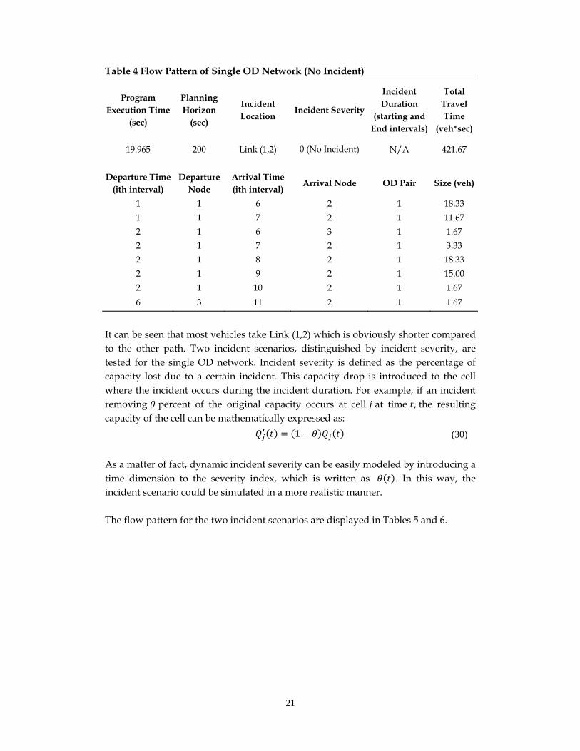
Table 4 Flow Pattern of Single OD Network (No Incident)

Program Execution Time

(sec)

Planning Horizon

(sec)

Incident Location

Incident Severity

Incident Duration

(starting and End intervals)

Total Travel Time

(veh*sec)

19.965 200 Link (1,2) 0 (No Incident) N/A 421.67

Departure Time (ith interval)

Departure Node

Arrival Time (ith interval)

Arrival Node OD Pair Size (veh)

1 1 6 2 1 18.33

1 1 7 2 1 11.67

2 1 6 3 1 1.67

2 1 7 2 1 3.33

2 1 8 2 1 18.33

2 1 9 2 1 15.00

2 1 10 2 1 1.67

6 3 11 2 1 1.67

It can be seen that most vehicles take Link (1,2) which is obviously shorter compared to the other path. Two incident scenarios, distinguished by incident severity, are tested for the single OD network. Incident severity is defined as the percentage of capacity lost due to a certain incident. This capacity drop is introduced to the cell where the incident occurs during the incident duration. For example, if an incident removing percent of the original capacity occurs at cell at time , the resulting capacity of the cell can be mathematically expressed as:

1 (30)

As a matter of fact, dynamic incident severity can be easily modeled by introducing a time dimension to the severity index, which is written as . In this way, the incident scenario could be simulated in a more realistic manner. The flow pattern for the two incident scenarios are displayed in Tables 5 and 6.

22

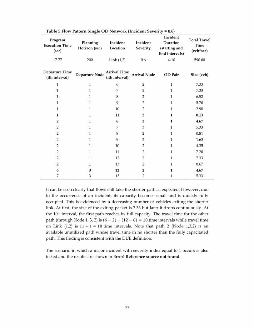
Table 5 Flow Pattern Single OD Network (Incident Severity = 0.6)


(sec)

Planning Horizon (sec)

Incident Location

Incident Severity

Incident Duration


Total Travel Time

(veh*sec)

17.77 200 Link (1,2) 0.6 4-10 590.00


Departure Node Arrival Time (ith interval)


1 1 6 2 1 7.33

1 1 7 2 1 7.33

1 1 8 2 1 6.52

1 1 9 2 1 5.70

1 1 10 2 1 2.98

1 1 11 2 1 0.13

2 1 6 3 1 4.67

2 1 7 3 1 5.33

2 1 8 2 1 0.81

2 1 9 2 1 1.63

2 1 10 2 1 4.35

2 1 11 2 1 7.20

2 1 12 2 1 7.33

2 1 13 2 1 8.67

6 3 12 2 1 4.67 7 3 13 2 1 5.33

It can be seen clearly that flows still take the shorter path as expected. However, due to the occurrence of an incident, its capacity becomes small and is quickly fully occupied. This is evidenced by a decreasing number of vehicles exiting the shorter link. At first, the size of the exiting packet is 7.33 but later it drops continuously. At the 10th interval, the first path reaches its full capacity. The travel time for the other path (through Node 1, 3, 2) is 6 2 12 6 10 time intervals while travel time on Link (1,2) is 11 1 10 time intervals. Note that path 2 (Node 1,3,2) is an available unutilized path whose travel time in no shorter than the fully capacitated path. This finding is consistent with the DUE definition. The scenario in which a major incident with severity index equal to 1 occurs is also tested and the results are shown in Error! Reference source not found..

23

Table 6 Flow Pattern of Single OD Network (Incident Severity = 1)


(sec)


Incident Location

Incident Severity

Incident Duration


Total Travel Time

(veh*sec)

35.87 200 Link (1,2) 1 4-10 536.67


Departure Node


Arrival Node

OD Pair Size (veh)

1 1 6 2 1 18.33

1 1 7 2 1 11.67

2 1 6 3 1 10.00

2 1 7 2 1 3.33

2 1 7 3 1 8.33

2 1 12 2 1 18.33

6 3 11 2 1 8.33

6 3 12 2 1 1.67

7 3 12 2 1 8.33

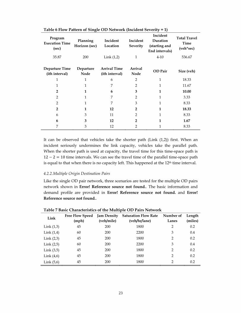
It can be observed that vehicles take the shorter path (Link (1,2)) first. When an incident seriously undermines the link capacity, vehicles take the parallel path. When the shorter path is used at capacity, the travel time for this time-space path is 12 2 10 time intervals. We can see the travel time of the parallel time-space path is equal to that when there is no capacity left. This happened at the 12th time interval.

4.2.2. Multiple Origin Destination Pairs

Like the single OD pair network, three scenarios are tested for the multiple OD pairs network shown in Error! Reference source not found.. The basic information and demand profile are provided in Error! Reference source not found. and Error! Reference source not found.. Table 7 Basic Characteristics of the Multiple OD Pairs Network

Link Free Flow Speed

(mph) Jam Density (veh/mile)

Saturation Flow Rate (veh/hr/lane)

Number of Lanes

Length (miles)

Link (1,3) 45 200 1800 2 0.2

Link (1,4) 60 200 2200 3 0.4

Link (2,3) 45 200 1800 2 0.2

Link (2,5) 60 200 2200 3 0.4

Link (3,5) 45 200 1800 2 0.2

Link (4,6) 45 200 1800 2 0.2

Link (5,6) 45 200 1800 2 0.2

24

Table 8 Demand Profile for Multiple OD Pairs Network Time Interval (sec) 10

Generation Node Generation Time

(ith interval) OD Pair Number of Vehicles

1 1 (1,6) 20

1 2 (1,6) 25

2 1 (2,6) 15

2 3 (2,6) 25

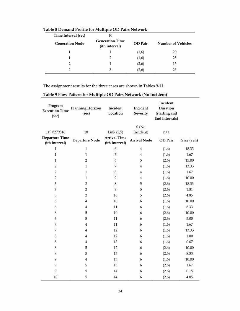
The assignment results for the three cases are shown in Tables 9-11.

Table 9 Flow Pattern for Multiple OD Pairs Network (No Incident)


(sec)


Incident Location

Incident Severity

Incident Duration


119.8279816 18 Link (2,5) 0 (No

Incident) n/a




1 1 6 4 (1,6) 18.33

1 1 7 4 (1,6) 1.67

1 2 6 5 (2,6) 15.00

2 1 7 4 (1,6) 13.33

2 1 8 4 (1,6) 1.67

2 1 9 4 (1,6) 10.00

3 2 8 5 (2,6) 18.33

3 2 9 5 (2,6) 1.81

3 2 10 5 (2,6) 4.85

6 4 10 6 (1,6) 10.00

6 4 11 6 (1,6) 8.33

6 5 10 6 (2,6) 10.00

6 5 11 6 (2,6) 5.00

7 4 11 6 (1,6) 1.67

7 4 12 6 (1,6) 13.33

8 4 12 6 (1,6) 1.00

8 4 13 6 (1,6) 0.67

8 5 12 6 (2,6) 10.00

8 5 13 6 (2,6) 8.33

9 4 13 6 (1,6) 10.00

9 5 13 6 (2,6) 1.67

9 5 14 6 (2,6) 0.15

10 5 14 6 (2,6) 4.85

25

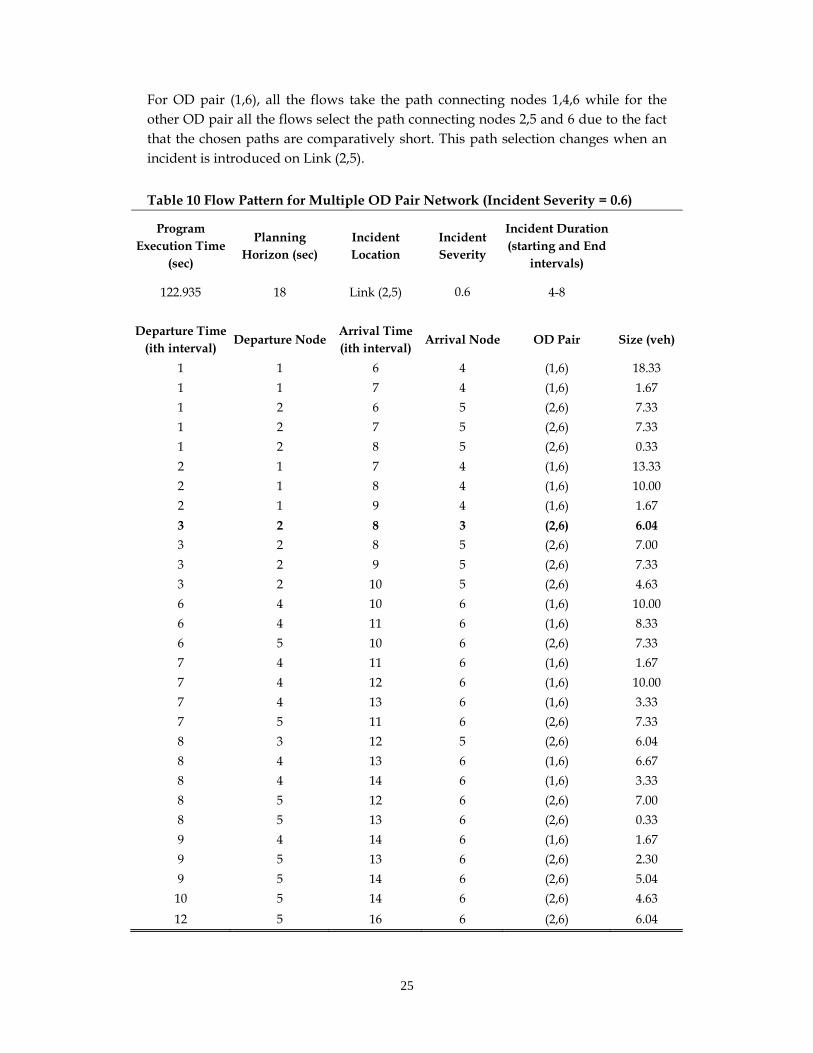
For OD pair (1,6), all the flows take the path connecting nodes 1,4,6 while for the other OD pair all the flows select the path connecting nodes 2,5 and 6 due to the fact that the chosen paths are comparatively short. This path selection changes when an incident is introduced on Link (2,5).

Table 10 Flow Pattern for Multiple OD Pair Network (Incident Severity = 0.6)


(sec)


Incident Location

Incident Severity

Incident Duration (starting and End

intervals)

122.935 18 Link (2,5) 0.6 4-8




1 1 6 4 (1,6) 18.33

1 1 7 4 (1,6) 1.67

1 2 6 5 (2,6) 7.33

1 2 7 5 (2,6) 7.33

1 2 8 5 (2,6) 0.33

2 1 7 4 (1,6) 13.33

2 1 8 4 (1,6) 10.00

2 1 9 4 (1,6) 1.67

3 2 8 3 (2,6) 6.04

3 2 8 5 (2,6) 7.00

3 2 9 5 (2,6) 7.33

3 2 10 5 (2,6) 4.63

6 4 10 6 (1,6) 10.00

6 4 11 6 (1,6) 8.33

6 5 10 6 (2,6) 7.33

7 4 11 6 (1,6) 1.67

7 4 12 6 (1,6) 10.00

7 4 13 6 (1,6) 3.33

7 5 11 6 (2,6) 7.33

8 3 12 5 (2,6) 6.04

8 4 13 6 (1,6) 6.67

8 4 14 6 (1,6) 3.33

8 5 12 6 (2,6) 7.00

8 5 13 6 (2,6) 0.33

9 4 14 6 (1,6) 1.67

9 5 13 6 (2,6) 2.30

9 5 14 6 (2,6) 5.04

10 5 14 6 (2,6) 4.63

12 5 16 6 (2,6) 6.04

26

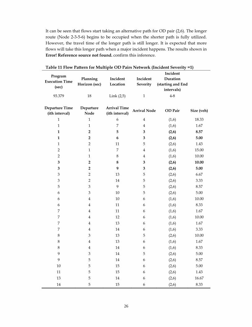
It can be seen that flows start taking an alternative path for OD pair (2,6). The longer route (Node 2-3-5-6) begins to be occupied when the shorter path is fully utilized. However, the travel time of the longer path is still longer. It is expected that more flows will take this longer path when a major incident happens. The results shown in Error! Reference source not found. confirm this inference. Table 11 Flow Pattern for Multiple OD Pairs Network (Incident Severity =1)


(sec)


Incident Location

Incident Severity

Incident Duration


93.379 18 Link (2,5) 1 4-8


Departure Node



1 1 6 4 (1,6) 18.33

1 1 7 4 (1,6) 1.67

1 2 5 3 (2,6) 8.57

1 2 6 3 (2,6) 5.00

1 2 11 5 (2,6) 1.43

2 1 7 4 (1,6) 15.00

2 1 8 4 (1,6) 10.00

3 2 8 3 (2,6) 10.00

3 2 9 3 (2,6) 5.00

3 2 13 5 (2,6) 6.67

3 2 14 5 (2,6) 3.33

5 3 9 5 (2,6) 8.57

6 3 10 5 (2,6) 5.00

6 4 10 6 (1,6) 10.00

6 4 11 6 (1,6) 8.33

7 4 11 6 (1,6) 1.67

7 4 12 6 (1,6) 10.00

7 4 13 6 (1,6) 1.67

7 4 14 6 (1,6) 3.33

8 3 13 5 (2,6) 10.00

8 4 13 6 (1,6) 1.67

8 4 14 6 (1,6) 8.33

9 3 14 5 (2,6) 5.00

9 5 14 6 (2,6) 8.57

10 5 15 6 (2,6) 5.00

11 5 15 6 (2,6) 1.43

13 5 14 6 (2,6) 16.67

14 5 15 6 (2,6) 8.33

27

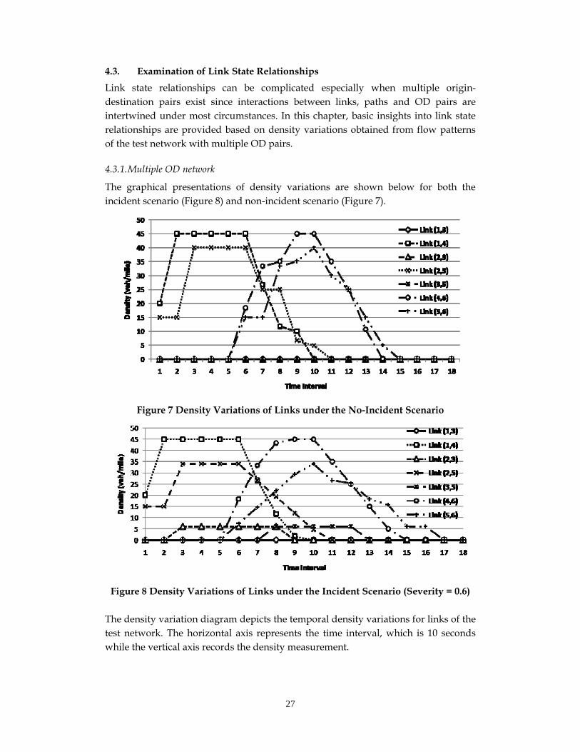
4.3. Examination of Link State Relationships

Link state relationships can be complicated especially when multiple origin-destination pairs exist since interactions between links, paths and OD pairs are intertwined under most circumstances. In this chapter, basic insights into link state relationships are provided based on density variations obtained from flow patterns of the test network with multiple OD pairs.

4.3.1. Multiple OD network

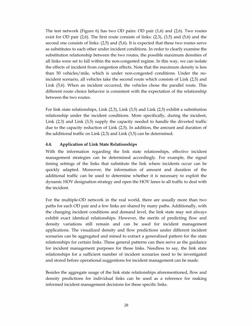
The graphical presentations of density variations are shown below for both the incident scenario (Figure 8) and non-incident scenario (Figure 7).

Figure 7 Density Variations of Links under the No-Incident Scenario

Figure 8 Density Variations of Links under the Incident Scenario (Severity = 0.6)

The density variation diagram depicts the temporal density variations for links of the test network. The horizontal axis represents the time interval, which is 10 seconds while the vertical axis records the density measurement.

28

The test network (Figure 6) has two OD pairs: OD pair (1,6) and (2,6). Two routes exist for OD pair (2,6). The first route consists of links: (2,3), (3,5) and (5,6) and the second one consists of links: (2,5) and (5,6). It is expected that these two routes serve as substitutes to each other under incident conditions. In order to clearly examine the substitution relationship between the two routes, the possible maximum densities of all links were set to fall within the non-congested regime. In this way, we can isolate the effects of incident from congestion effects. Note that the maximum density is less than 50 vehicles/mile, which is under non-congested conditions. Under the no-incident scenario, all vehicles take the second route which consists of Link (2,5) and Link (5,6). When an incident occurred, the vehicles chose the parallel route. This different route choice behavior is consistent with the expectation of the relationship between the two routes. For link state relationships, Link (2,3), Link (3,5) and Link (2,5) exhibit a substitution relationship under the incident conditions. More specifically, during the incident, Link (2,3) and Link (3,5) supply the capacity needed to handle the diverted traffic due to the capacity reduction of Link (2,5). In addition, the amount and duration of the additional traffic on Link (2,3) and Link (3,5) can be determined.

4.4. Application of Link State Relationships

With the information regarding the link state relationships, effective incident management strategies can be determined accordingly. For example, the signal timing settings of the links that substitute the link where incidents occur can be quickly adapted. Moreover, the information of amount and duration of the additional traffic can be used to determine whether it is necessary to exploit the dynamic HOV designation strategy and open the HOV lanes to all traffic to deal with the incident. For the multiple-OD network in the real world, there are usually more than two paths for each OD pair and a few links are shared by many paths. Additionally, with the changing incident conditions and demand level, the link state may not always exhibit exact identical relationships. However, the merits of predicting flow and density variations still remain and can be used for incident management applications. The visualized density and flow predictions under different incident scenarios can be aggregated and mined to extract a generalized pattern for the state relationships for certain links. These general patterns can then serve as the guidance for incident management purposes for those links. Needless to say, the link state relationships for a sufficient number of incident scenarios need to be investigated and stored before operational suggestions for incident management can be made. Besides the aggregate usage of the link state relationships aforementioned, flow and density predictions for individual links can be used as a reference for making informed incident management decisions for these specific links.

29

Chapter 5 Conclusions and Future Extensions

5.1. Conclusions

Effective implementation of incident mitigation strategies requires accurate and efficient procedures to predict link states, which are described by traffic density and flow. Considering the diversion behavior and the characteristics of link states, in this project, we apply UE-DTA to predict the link states and get insights regarding link state relationships. We developed a linear programming model that incorporates multiple origin destination pairs while possessing the capability of modeling transient incident phenomena. The model is based on the LP-DTA framework proposed by other researchers which allows user equilibrium by iterating between an upper level and lower level program that constitute the whole model. The model’s equivalence to DUE is proved by exploiting the Kuhn-Tucker condition, which is necessary and sufficient for a linear program. Two cases, namely the single OD pair network and multiple OD network, were constructed and tested. The results show that the flow pattern preserves the user equilibrium principle and satisfies the FIFO condition. The link-based encapsulation of Cell Transmission Model is able to temporally capture the spillback between links and fully mimics the spillback within links. This model strikes a balance between computational tractability, traffic realism and incident modeling capability. The flow pattern resultant from the model can be easily transformed to link density variations as shown in Section 4.3. The prediction of link density variations, combined with the flow pattern, is used to investigate the link state relationships. By isolating the effects of incident occurrence, the parallel routes of a specific OD pair display the relationship of substituting for each other, which is consistent with the general expectation regarding such parallel routes. A closer examination over the density variations confirms the existence of a substitution relationship between the links of the two parallel routes. Detailed information about the additional traffic on the diversion route is also obtained. Two levels of application of link state relationships are identified for real-world situations. Information about link states for different incident scenarios can be aggregated and mined to derive general patterns for the link state relationships. These patterns can be used as general guidance for incident management purposes. A microscopic level of application involves usage of flow and density predictions for a specific incident. For example, they can be used to determine whether it is necessary to exploit the dynamic HOV designation strategy and open the HOV lane to all traffic to deal with the incident. Operational adjustments such as changing signal timing can also be made based on the information regarding link states.

30

5.2. Future Extensions

One of the most important extensions is apparently to deal with spatial spillbacks between links. In the lower level CTM model, when diverge and merge cells are introduced, it is critical to come up with a mechanism to determine the diverge coefficients while maintaining the FIFO condition. In addition, real-world situations including queuing at signalized intersections can be also incorporated into the model by adapting the lower level CTM model. More specifically, cell capacities can be set as time-dependent to simulate the traffic signals. With these extensions and adaption, the model can be applied to large-scale networks by refining the solution code or resorting to more advanced computing techniques. Another avenue for future research is to explore how to integrate the information about link state relationships under different incident scenarios and thus derive the general pattern of link state relationships. High computation speed for this derivation process is desired since incident mitigation strategies need to be determined quickly. Therefore, research efforts are needed in the aspects such as designing efficient data mining algorithms for real-time deployment.

31

References

Bertsekas, D. (1999). Nonlinear Programming. Belmont Massachusetts, Athena Scientific.

Cambridge Systematics, I. (2005). "Traffic Congestion and Reliability: Trends and Advanced Strategies for Congestion Mitigation." Retrieved September 23, 2009, from http://ops.fhwa.dot.gov/congestion_report/.

Carey, M. (1999). A Framework for Dynamic Traffic Assignment. Northern Ireland, University of Ulster.

Carey, M. (2009). "A framework for user equilibrium dynamic traffic assignment." Journal of the Operational Research Society 60: 395-410.

Carey, M. and E. Subrahmanian (2000). "An approach to modelling time-varying flows on congested networks." Transportation Research, Part B (Methodological) 34B(3): 157-183.

Dafermos, S. (1980). "Traffic equilibrium and variational inequalities." Transportation Science 14(Copyright 1980, IEE): 42-54.

Daganzo, C. F. (1994). "The cell transmission model: a dynamic representation of highway traffic consistent with the hydrodynamic theory." Transportation Research, Part B (Methodological) 28B(4): 269-287.

Daganzo, C. F. (1995). "The cell transmission model. II. Network traffic." Transportation Research, Part B (Methodological) 29B(2): 79-93.

Friesz, T. L., J. Luque, et al. (1989). "Dynamic network traffic assignment considered as a continuous time optimal control problem." Operations Research 37(6): 893-901.

Ge, Y. E. and M. Carey (2004). Travel time computation of link and path flows and first-in-first-out, Dalian, China, Science Press.

Golani, H. and S. T. Waller (2004). "Combinatorial approach for multiple-destination user optimal dynamic traffic assignment." Transportation Research Record(1882): 70-78.

Helman, D. L. (2004). "Traffic Incident Management." Retrieved September 23, 2009, from http://www.tfhrc.gov/pubrds/04nov/03.htm.

Huey-Kuo, C. and H. Che-Fu (1998). "A model and an algorithm for the dynamic user-optimal route choice problem." Transportation Research, Part B (Methodological) 32B(Copyright 1998, IEE): 219-234.

Janson, B. N. (1991a). "Dynamic traffic assignment for urban road networks." Transportation Research, Part B (Methodological) 25B: 143-161.

Janson, B. N. (1991b). "Convergent Algorithm for Dynamic Traffic Assignment." Transportation Research Record 1328: 69-80.

Jayakrishnan, R., A. Chen, et al. (1999). "Freeway and arterial traffic flow simulation analytically embedded in dynamic assignment." Transportation Research Record(1678): 242-250.

Jayakrishnan, R., W. K. Tsai, et al. (1995). "A dynamic traffic assignment model with traffic-flow relationships." Transportation Research Part C (Emerging Technologies) 3C(1): 51-72.

32

Li, Y., A. K. Ziliaskopoulos, et al. (1999). "Linear programming formulations for system optimum dynamic traffic assignment with arrival time-based and departure time-based demands." Transportation Research Record(1667): 52-59.

Lighthill, M. J. and G. B. Whitham (1955). "On kinematic waves, Theory of traffic flow on long crowded roads." Proceedings of Royal Society of London 229(1178): 317-345.

Liu, S. and P. Murray-Tuite (2008). Evaluation of Stategies to Increase Transportation Resilience to Congestion Caused by Incidents. Falls Church, Virginia, Virginia Polytechnic and State University.

Lo, H. K. and W. Y. Szeto (2002). "A cell-based dynamic traffic assignment model: Formulation and properties." Mathematical and Computer Modelling 35(7-8): 849-865.

Merchant, D. K. and G. L. Nemhauser (1978a). "A Model and an Algorithm for the Dynamic Traffic Assignment Problems." Transportation Science 12(3): 183-199.

Merchant, D. K. and G. L. Nemhauser (1978b). "Optimality Conditions for a Dynamic Traffic Assignment Model." Transportation Science 12(3): 200-207.

Peeta, S. and A. K. Ziliaskopoulos (2001). "Foundations of Dynamic Traffic Assignment: The past, the present and the future." Networks and Spatial Economics 1(3-4): 233-265.

Ran Bin and D. Boyce (1994). Dynamic Urban Transportation Network Models: Theory and Implications for Intelligent Vehicle Highway Systems. Berlin, Springer-Verlag.

Richards, P. I. (1956). "Shock waves on highway." Operations Research Society of America -- Journal 4(1): 42-51.

Robinson, M. D. and P. M. Nowak (1993). "An Overview of Freeway Incident Management in the United States."

Sheffi, Y. (1985). Urban Transportation Networks: Equilibrium Analysis with Mathematical Programming Methods. Englewood Cliffs, New Jersey, Prentice-Hall.

Waller, S. T. and A. Ziliaskopoulos (2006). "A combinatorial user optimal dynamic traffic assignment algorithm." Annals of Operations Research 144: 249-261.

Waller, S. T. and A. K. Ziliaskopoulos (2006). "A chance-constrained based stochastic dynamic traffic assignment model: Analysis, formulation and solution algorithms." Transportation Research Part C (Emerging Technologies) 14(6): 418-427.

Ziliaskopoulos, A. K. (2000). "A linear programming model for the single destination system optimum dynamic traffic assignment problem." Transportation Science 34(1): 37-49.

Documents

LINK STATE RELATIONSHIPS UNDER INCIDENT · PDF fileLINK STATE RELATIONSHIPS UNDER INCIDENT CONDITIONS: USING A CTM-BASED LINEAR PROGRAMMING DYNAMIC ... The effectiveness of these