Embed Size (px)
Citation preview

CHAPTER III
LINEAR SYSTEM RESPONSE
31 OBJECTIVES
The output produced by an operational amplifier (or any other dynamic system) in response to a particular type or class of inputs normally proshyvides the most important characterization of the system The purpose of this chapter is to develop the analytic tools necessary to determine the reshysponse of a system to a specified input
While it is always possible to determine the response of a linear system to a given input exactly we shall frequently find that greater insight into the design process results when a system response is approximated by the known response of a simpler configuration For example when designing a low-level preamplifier intended for audio signals we might be interested in keeping the frequency response of the amplifier within i 5 of its mid-band value over a particular bandwidth If it is possible to approximate the amplifier as a two- or three-pole system the necessary constraints on pole location are relatively straightforward Similarly if an oscilloscope vertical amplifier is to be designed a required specification might be that the overshyshoot of the amplifier output in response to a step input be less than 3 of its final value Again simple constraints result if the system transfer function can be approximated by three or fewer poles
The advantages of approximating the transfer functions of linear systems can only be appreciated with the aid of examples The LM301A integrated-circuit operational amplifier has 13 transistors included-in its signal-transshymission path Since each transistor can be modeled as having two capacishytors the transfer function of the amplifier must include 26 poles Even this estimate is optimistic since there is distributed capacitance comparable to transistor capacitances associated with all of the other components in the signal path
Fortunately experimental measurements of performance can save us from the conclusion that this amplifier is analytically intractable Figure 3la shows the LM301A connected as a unity-gain inverter Figures 31b and 3lc show the output of this amplifier with the input a -50-mV step
1This amplifier is described in Section 1041
63
64 Linear System Response
47 kn
47 k
V F -+ V LM301 A 0 -
Compensating capacitor
(a)
20 mV
(b) 2 AsK
Figure 31 Step responses of inverting amplifier (a) Connection (b) Step response
with 220-pF compensating capacitor (c) Step response with 12-pF compensating
capacitor
for two different values of compensating capacitor2 The responses of an
R-C network and an R-L-C network when excited with +50-mV steps
supplied from the same generator used to obtain the previous transients
are shown in Figs 32a and 32b respectively The network transfer funcshy
tions are V0(s) 1 Vi(s) 25 X 10- 6 s + I
Objectives 65
20 mV
(c) 05 yAs
Figure 31-Continued
for the response shown in Fig 32a and
V0(s) 1 1 2Vi(s) 25 X 104 s + 7 X 10- 8s + I
for that shown in Fig 32b We conclude that there are many applications where the first- and second-order transfer functions of Eqns 31 and 32 adequately model the closed-loop transfer function of the LM301A when connected and compensated as shown in Fig 31
This same type of modeling process can also be used to approximate the open-loop transfer function of the operational amplifier itself Assume that the input impedance of the LM301A is large compared to 47 ki and that its output impedance is small compared to this value at frequencies of interest The closed-loop transfer function for the connection shown in Fig 31 is then
V0(s) -a(s) Vi(s) 2 + a(s)
2 Compensation is a process by which the response of a system can be modified advanshytageously and is described in detail in subsequent sections
20 mV
T
(a) 2 S
20 mV
(b) 05 s
Figure 32 Step responses for first- and second-order networks (a) Step response for V(s)Vi(s) = ](25 X 10- 6s + 1) (b) Step response for V(s)Vi(s) =
S2 81(25 X 10 14 + 7 X 10 s + 1)
66
67 Laplace Transforms
where a(s) is the unloaded open-loop transfer function of the amplifier Substituting approximate values for closed-loop gain (the negatives of Eqns 31 and 32) into Eqn 33 and solving for a(s) yields
a~) 8 X 10⁵ a(s) 8X(34)
and
28 X 107 a(s) 2 0 (35)s(35 X 10- 7 s + 1)
as approximate open-loop gains for the amplifier when compensated with 220-pF and 12-pF capacitors respectively We shall see that these approxishymate values are quite accurate at frequencies where the magnitude of the loop transmission is near unity
32 LAPLACE TRANSFORMS3
Laplace Transforms offer a method for solving any linear time-invariant differential equation and thus can be used to evaluate the response of a linear system to an arbitrary input Since it is assumed that most readers have had some contact with this subject and since we do not intend to use this method as our primary analytic tool the exposure presented here is brief and directed mainly toward introducing notation and definitions that will be used later
321 Definitions and Properties
The Laplace transform of a time functionf(t) is defined as
2[f(t)] A F(s) A f f(t)e- dt (36)
where s is a complex variable o + jw The inverse Laplace transform of the complex function F(s) is
-1[F(s)]A f(t) A F(s)e ds (37)2rj 1-J Fs d
A complete discussion is presented in M F Gardner and J L Barnes Transientsin LinearSystems Wiley New York 1942
In this section we temporarily suspend the variable and subscript notation used elseshywhere and conform to tradition by using a lower-case variable to signify a time function and the corresponding capital for its transform
68 Linear System Response
The direct-inverse transform pair is unique4 so that
2-12[ftt)] =f (t (38)
iff(t) = 0 t lt 0 and if f f(t) | e- dt is finite for some real value of a1
A number of theorems useful for the analysis of dynamic systems can be developed from the definitions of the direct and inverse transforms for functions that satisfy the conditions of Eqn 38 The more important of these theorems include the following
1 Linearity 2[af(t) + bg(t)] = [aF(s) + bG(s)]
where a and b are constants
2 Differentiation
Ldf(t) sF(s) - lim f(t)dt =-0+
(The limit is taken by approaching t = 0 from positive t)
3 Integration
2 [ f(T) d-] F(s)
4 Convolution
2 [f tf(r)g(t - r) d] = [ ff(t - r)g(r) dr] = F(s)G(s)
5 Time shift 2[f(t - r)] = F(s)e-
if f(t - r) = 0 for (t - r) lt 0 where r is a positive constant
6 Time scale
1 Fs]2[f(at)] = F -shy
a a
where a is a positive constant
7 Initialvalue lim f(t) lim sF(s) t-0+ 8-co
4 There are three additional constraints called the Direchlet conditions that are satisfied
for all signals of physical origin The interested reader is referred to Gardner and Barnes
69 Laplace Transforms
8 Final value
limf (t) = lim sF(s) J-oo 8-0
Theorem 4 is particularly valuable for the analysis of linear systemssince it shows that the Laplace transform of a system output is the prodshyuct of the transform of the input signal and the transform of the impulse response of the system
322 Transforms of Common Functions
The defining integrals can always be used to convert from a time funcshytion to its transform or vice versa In practice tabulated values are freshyquently used for convenience and many mathematical or engineering refshyerencesI contain extensive lists of time functions and corresponding Laplace transforms A short list of Laplace transforms is presented in Table 31
The time functions corresponding to ratios of polynomials in s that are not listed in the table can be evaluated by means of a partialfraction exshypansion The function of interest is written in the form
F(s) = p(s) _ p(s)q(s) (s + s1 )(s + s2) (s + s)
It is assumed that the order of the numerator polynomial is less than that of the denominator If all of the roots of the denominator polynomial are first order (ie s si i j)
F(s) = (310) k=1 S + sk
where
Ak = lim [(s + sk)F(s)] (311) k
If one or more roots of the denominator polynomial are multiple roots they contribute terms of the form
ZBkk- BsI~k + (312)
k1(S Si) k
See for example A Erdeyli (Editor) Tables of Integral Transforms Vol 1 Bateman Manuscript Project McGraw-Hill New York 1954 and R E Boly and G L Tuve (Editors) Handbook of Tables for Applied Engineering Science The Chemical Rubber Company Cleveland 1970
70 Linear System Response
Table 31 Laplace Transform Pairs
f(t) t gt 0F(s)
[f(t) = 0 t lt 0]
1 Unit impulse uo(t)
1 Unit step u-1 (t)
S2 [f(t) = 1 t gt 0]
1 Unit ramp u- 2(t)
[f(t) = t t gt 0]
1 tn
s+1a n
e-at s + a1
1 tn Se-at
(s + a)+1 (n)
1 1 - e-t
s(rs + 1
e-a sin wt(s + a)2 + W2
s + a e-a cos Wt (s + a)2 + W22
1 on 2 e-t-wn(sin 1 - -2 t) lt 1 s2 + 2 sn + 1 1 - 2
1 1 - sin coV1 - 2 t + tan- 22s(s 2 O2 + sWn + 1)
where m is the order of the multiple root located at s = -si The Bs are determined from the relationship
Bk = lim [(s + si)-F(s)] (313)k) ds--k8 (m( shy
71 Laplace Transforms
Because of the linearity property of Laplace transforms it is possible to find the time function f(t) by summing the contributions of all components of F(s)
The properties of Laplace transforms listed earlier can often be used to determine the transform of time functions not listed in the table The recshytangular pulse shown in Fig 33 provides one example of this technique The pulse (Fig 33a) can be decomposed into two steps one with an amplitude of +A starting at t = ti summed with a second step of amplishy
tl t 2
t 3P
(a)
f(t)
A
0 tl
-A -------shy
(b)
Figure 33 Rectangular pulse (a) Signal (b) Signal decomposed in two steps
72 Linear System Response
sin wt 0 lt t lt 0 otherwise
(a)
f(t)
sin wt t gt 0 sin w(t -) (t -)gt 0
01
11
(b)
Figure 34 Sinusoidal pulse (a) Signal (b) Signal decomposed into two sinusoids
(c) First derivative of signal (d) Second derivative of signal
tude - A starting at t = t 2 Theorems 1 and 5 combined with the transform of a unit step from Table 31 show that the transform of a step with amplishytude A that starts at t = ti is (As)e-I Similarly the transform of the second component is -(As)e- Superposition insures that the transform of f(t) is the sum of these two functions or
F(s) = (e- t - e-s2) (314) S
The sinusoidal pulse shown in Fig 34 is used as a second example
One approach is to represent the single pulse as the sum of two sinusoids
73 Laplace Tranforms
f(t)
w cos wt 0 lt t lt 0 otherwise
0
(c)
ft f1(t)
Impulse of area o
0 t al
-W 2 sin cot 0 lt t lt 1 0 otherwise
(d) Figure 34--Continued
exactly as was done for the rectangular pulse Table 31 shows that the transform of a unit-amplitude sinusoid starting at time t = 0 is w(s2 plusmn w2) Summing transforms of the components shown in Fig 3 4b yields
F(s) = 2 2 [I+e- ] (315) s2 + O
An alternative approach involves differentiating f(t) twice The derivative of f(t) f(t) is shown in Fig 34c Since f(0) = 0 theorem 2 shows that
2[f(t)] = sF(s) (316)
74 Linear System Response
The second derivative of f(t) is shown in Fig 34d Application of theorem 2 to this function 6 leads to
2[f(t)] = s2[f(t)] - lim f(t) = s 2F(s) - w (317) t- 0+
However Fig 34d indicates that
f(t) = -W 2f(t) + wuo t - -) (318)
Thus = -C 2F(s) + we--(w) (319)
Combining Eqns 317 and 319 yields
s2F(s) - o = --C2F(s) + coe-(Iw) (320)
Equation 320 is solved for F(s) with the result that
F(s) = + [1 + e-(wgt] (321)s 2 + W2
Note that this development in contrast to the one involving superposition does not rely on knowledge of the transform of a sinusoid and can even be used to determine this transform
323 Examples of the Use of Transforms
Laplace transforms offer a convenient method for the solution of linear time-invariant differential equations since they replace the integration and differentiation required to solve these equations in the time domain by algebraic manipulation As an example consider the differential equation
d2x dx + 3 + 2x = e-I t gt 0 (322)
dt 2 dt
subject to the initial conditions
dx x(0+) = 2 (0+) = 0
dt
The transform of both sides of Eqn 322 is taken using theorem 2 (applied twice in the case of the second derivative) and Table 31 to determine the Laplace transform of e-
s2X(s) - sx(0+) -dx
(0+) + 3sX(s) - 3x(0+) + 2X(s) - (323)dt s + 1
6The portion of this expression involving lim t-0+could be eliminated if a second imshypulse wuo(t) were included in f (t)
75 Laplace Transforms
5 0
(s) = (s + 1)(07 X 10-6S + 1)
Figure 35 Unity-gain follower
Collecting terms and solving for X(s) yields
2s2 + 8s + 7 (s + 1)2(s + 2)
Equations 310 and 312 show that since there is one first-order root and one second-order root
A1 B1 B2X(S) = A + B + B2(325)(s + 2) (s + 1) (s + 1)2
The coefficients are evaluated with the aid of Eqns 311 and 313 with the result that
--1 3 1 X(S) = + + (326)
s + 2 s + I (s + 1)2
The inverse transform of X(s) evaluated with the aid of Table 31 is
te tx(t) = -e-21 + 3e- + (327)
The operational amplifier connected as a unity-gain noninverting amplishyfier (Fig 35) is used as a second example illustrating Laplace techniques If we assume loading is negligible
VJ(s) a(s) 7 X 10⁵
Vi(s) I + a(s) (s + 1)(07 X 10- 6s + 1) + 7 X 101
10-12s 2 + 14 X 10- 6 s + 1 (328)
If the input signal is a unit step so that Vi(s) is 1s
V 6(s) = 2 I
s(10-12s + 14 X 10-6s + 1)
s[s2(10 6)2 + 2(07)s106 + 1] (329)
76 Linear System Response
The final term in Eqn 329 shows that the quadratic portion of the exshypression has a natural frequency w = 106 and a damping ratio = 07 The corresponding time function is determined from Table 31 with the result
)-07104t
f(t) = 1 -(
sin (07 X 106 t + 450) (330)
07
33 TRANSIENT RESPONSE
The transientresponse of an element or system is its output as a function of time following the application of a specified input The test signal chosen to excite the transient response of the system may be either an input that is anticipated in normal operation or it may be a mathematical abstracshytion selected because of the insight it lends to system behavior Commonly used test signals include the impulse and time integrals of this function
331 Selection of Test Inputs
The mathematics of linear systems insures that the same system inforshymation is obtainable independent of the test input used since the transfer function of a system is clearly independent of inputs applied to the system In practice however we frequently find that certain aspects of system pershyformance are most easily evaluated by selecting the test input to accentuate features of interest
For example we might attempt to evaluate the d-c gain of an operational amplifier with feedback by exciting it with an impulse and measuring the net area under the impulse response of the amplifier This approach is mathematically sound as shown by the following development Assume that the closed-loop transfer function of the amplifier is G(s) and that the corresponding impulse response [the inverse transform of G(s)] is g(t) The properties of Laplace transforms show that
f 0 g(t) dt = - G(s) (331)S
The final value theorem applied to this function indicates that the net area under impulse response is
lim g(t) dt = lim s - G(s) = G(0) (332) t-c o s-0
Unfortunately this technique involves experimental pitfalls The first of these is the choice of the time function used to approximate an impulse
77 Transient Response
In order for a finite-duration pulse to approximate an impulse satisfactorily it is necessary to have
t sm I (333)
where t is the width of the pulse and sm is the frequency of the pole of G(s) that is located furthest from the origin
It may be difficult to find a pulse generator that produces pulses narrow enough to test high-frequency amplifiers Furthermore the narrow pulse frequently leads to a small-amplitude output with attendant measurement problems Even if a satisfactory impulse response is obtained the tedious task of integrating this response (possibly by counting boxes under the output display on an oscilloscope) remains It should be evident that a far more accurate and direct measurement of d-c gain is possible if a conshystant input is applied to the amplifier
Alternatively high-frequency components of the system response are not excited significantly if slowly time-varying inputs are applied as test inputs In fact systems may have high-frequency poles close to the imaginary axis in the s-plane and thus border on instability yet they exhibit well-behaved outputs when tested with slowly-varying inputs
For systems that have neither a zero-frequency pole nor a zero in their transfer function the step response often provides the most meaningful evaluation of performance The d-c gain can be obtained directly by measuring the final value of the response to a unit step while the initial discontinuity characteristic of a step excites high-frequency poles in the system transfer function Adequate approximations to an ideal step are provided by rectangular pulses with risetimes
t ltlt s (334)
(sm as defined earlier) and widths
t gtgt - (335)
where s is the frequency of the pole in the transfer function located closest to the origin Pulse generators with risetimes under I ns are available and these generators can provide useful information about amplifiers with bandwidths on the order of 100 MHz
I While this statement is true in general if only the d-c gain of the system is required any pulse can be used An extension of the above development shows that the area under the response to any unit-area input is identical to the area under the impulse response
78 Linear System Response
332 Approximating Transient Responses
Examples in Section 31 indicated that in some cases it is possible to approximate the transient response of a complex system by using that of a much simpler system This type of approximation is possible whenever the transfer function of interest is dominated by one or two poles
Consider an amplifier with a transfer function
aom (rzis + 1) V =(s) n gt m all r gt 0 (336)Vt(s) T (rpjs + 1)
j= 1
The response of this system to a unit-step input is
F1 V0(s) 1 v0 t) = 2--1 -I- a + $ AketTpk (337)
s V(s) k=1
The As obtained from Eqn 311 after slight rearrangement are
H -z +1
A - + ) (338)
Tk3c
Assume thatTri gtgt all other rs In this case which corresponds to one pole in the system transfer function being much closer to the origin than all other singularities Eqn 338 can be used to show that A1 ~ ao and all other As - 0 so that
v(t) ~ ao(l - e-rPi) (339)
This single-exponential transient response is shown in Fig 36 Experience shows that the single-pole response is a good approximation to the actual response if remote singularities are a factor of five further from the origin than the dominant pole
The approximate result given above holds even if some of the remote singularities occur in complex conjugate pairs providing that the pairs are located at much greater distances from the origin in the s plane than the dominant pole However if the real part of the complex pair is not more negative than the location of the dominant pole small-amplitude high-frequency damped sinusoids may persist after the dominant transient is completed
79 Transient Response
i i----_
(1 - 1) - 063 ---
0 1 t P1
Figure 36 Step response of first-order system
Another common singularity pattern includes a complex pair of poles much closer to the origin in the s plane than all other poles and zeros An argument similar to that given above shows that the transfer function of an amplifier with this type of singularity pattern can be approximated by the complex pair alone and can be written in the standard form
V0(s) a0V-(S)- a(340)Vs(s) s2W 2 + 2 sw + 1
The equation parameters w and are called the naturalfrequency(expressed in radians per second) and the damping ratio respectively The physical significance of these parameters is indicated in the s-plane plot shown as Fig 37 The relative pole locations shown in this diagram correspond to the underdamped case ( lt 1) Two other possibilities are the critically damped pair ( = 1) where the two poles coincide on the real axis and the overdampedcase ( gt 1) where the two poles are separated on the real axis The denominator polynomial can be factored into two roots with real coefficients for the later two cases and as a result the form shown in Eqn 340 is normally not used The output provided by the amplifier described by Eqn 340 in response to a unit step is (from Table 31)
vO(t) = ao 1 - 1 en t sin (1 - 2 t + ltp)] (341)
where
D= tan-yV- 2]
80 Linear System Response
Location of pole pair n s plane
0 = cos-l9
a = Re(s)-shy
X
Figure 37 s-plane plot of complex pole pair
Figure 38 is a plot of v0(t) as a function of normalized time wat for various values of damping ratio Smaller damping ratios corresponding to comshyplex pole pairs with the poles nearer the imaginary axis are associated with step responses having a greater degree of overshoot
The transient responses of third- and higher-order systems are not as
easily categorized as those of first- and second-order systems since more parameters are required to differentiate among the various possibilities The situation is simplified if the relative pole positions fall into certain patterns One class of transfer functions of interest are the Butterworth filters These transfer functions are also called maximally flat because of properties of their frequency responses (see Section 34) The step responses of Butterworth filters also exhibit fairly low overshoot and because of
these properties feedback amplifiers are at times compensated so that their closed-loop poles form a Butterworth configuration
The poles of an nth-order Butterworth filter are located on a circle censhy
tered at the origin of the s-plane For n even the poles make angles [ (2k + 1) 90 0n with the negative real axis where k takes all possible inshytegral values from 0 to (n2) - 1 For n odd one pole is located on the
negative real axis while others make angles of -k (180 0 n) with the negashy
tive real axis where k takes integral values from 1 to (n2) - (12) Thus
for example a first-order Butterworth filter has a single pole located at
s = - on The second-order Butterworth filter has its poles located I45 from the negative real axis corresponding to a damping ratio of 0707
81 Frequency Response
18 01
16 - 02
- 03 14 - 04
12 05 12 - - - -
vo ) - 0707 50
10 j
08 - -
06 r-=
04 shy
02
0 I I | | | | | I 0 2 4 6 8 10 12 14 16 18 20 22 24
Figure 38 Step responses of second-order system
The transfer functions for third- and fourth-order Butterworth filters are
BAS) = s3W3 + 2s2co 2 + 2sw + 1 (342)
and
B4(s) = s4w 4 + 261s 3w 3 + 342s2o 2 + 261sw + 1 (343)
respectively Plots of the pole locations of these functions are shown in Fig 39 The transient outputs of these filters in response to unit steps are shown in Fig 310
34 FREQUENCY RESPONSE
The frequency response of an element or system is a measure of its steady-state performance under conditions of sinusoidal excitation In
I C(A
s plane
adius = co
a
s plane
Radius = con
a ~
(b)
Figure 39 Pole locations for third- and fourth-order Butterworth filters (a) Third-
Order (b) Fourth-order
82
83 Frequency Response
order
f 06 shyv 0 (t)
04 shy
02
0 0 2 4 6 8 10 12 14 16
wnt a
Figure 310 Step responses for third- and fourth-order Butterworth filters
steady state the output of a linear element excited with a sinusoid at a frequency w (expressed in radians per second) is purely sinusoidal at freshyquency w The frequency response is expressed as a gain or magnitude M(w) that is the ratio of the amplitude of the output to the input sinusoid and a phase angle 4(co) that is the relative angle between the output and input sinusoids The phase angle is positive if the output leads the input The two components that comprise the frequency response of a system with a transfer function G(s) are given by
M(co) = I G(jeo) (344a)
$(w) = 4G(j) tan- Im[G(jw)] (344b)Re[G(jo)]
It is frequently necessary to determine the frequency response of a sysshytem with a transfer function that is a ratio of polynomials in s One posshysible method is to evaluate the frequency response by substituting jW for s at all frequencies of interest but this method is cumbersome particularly for high-order polynomials An alternative approach is to present the inshyformation concerning the frequency response graphically as described below
18
84 Linear System Response
The transfer function is first factored so that both the numerator and denominator consist of products of first- and second-order terms with real coefficients The function can then be written in the general form
a s2 2 isG(s) (Ths + 1) 2 + s
S first- complex Wni Oni order zero
Lzeros J Lpairs
X H 2
(345) first- (rjS + 1) complex (S
2 nk + 2kSWnk + 1)
order pole Lpoles L-pairs
While several methods such as Lins method are available for factoring polynomials this operation can be tedious unless machine computation is employed particularly when the order of the polynomial is large Fortushynately in many cases of interest the polynomials are either of low order or are available from the system equations in factored form
Since G(jo) is a function of a complex variable its angle $(w) is the sum of the angles of the constituent terms Similarly its magnitude M(w) is the product of the magnitudes of the components Furthermore if the magnishytudes of the components are plotted on a logarithmic scale the log of M is given by the sum of the logs corresponding to the individual comshyponentsI
Plotting is simplified by recognizing that only four types of terms are possible in the representation of Eqn 345
1 Constants ao 2 Single- or multiple-order differentiations or integrations sn where n
can be positive (differentiations) or negative (integrations) 3 First-order terms (TS + 1) or its reciprocal
2 2 24 Complex conjugate pairs s + swn + 1 or its reciprocal
8 S N Lin A Method of Successive Approximations of Evaluating the Real and Comshy
plex Roots of Cubic and Higher-Order Equations J Math Phys Vol 20 No 3 August 1941 pp 231-242
9The decibel equal to 20 logio [magnitude] is often used for these manipulations This
usage is technically correct only if voltage gains or current gains between portions of a circuit with identical impedance levels are considered The issue is further confused when the decibel is used indiscriminately to express dimensioned quantities such as transconshyductances We shall normally reserve this type of presentation for loop-transmission manipulations (the loop transmission of any feedback system must be dimensionless) and simply plot signal ratios on logarithmic coordinates
85 Frequency Response
It is particularly convenient to represent each of these possible terms as a plot of M (on a logarithmic magnitude scale) and $ (expressed in degrees) as a function of o (expressed in radians per second) plotted on a logarithshymic frequency axis A logarithmic frequency axis is used because it provides adequate resolution in cases where the frequency range of interest is wide and because the relative shape of a particular response curve on the log axis does not change as it is frequency scaled The magnitude and angle of any rational function can then be determined by adding the magnitudes and angles of its components This representation of the frequency response of a system or element is called a Bode plot
The magnitude of a term ao is simply a frequency-independent constant with an angle equal to 00 or 1800 depending on whether the sign of ao is positive or negative respectively
Both differentiations and integrations are possible in feedback systems For example a first-order high-pass filter has a single zero at the origin and thus its voltage transfer ratio includes a factor s A motor (frequently used in mechanical feedback systems) includes a factor 1s in the transfer function that relates mechanical shaft angle to applied motor voltage since a constant input voltage causes unlimited shaft rotation Similarly various types of phase detectors are examples of purely electronic elements that have a pole at the origin in their transfer functions This pole results beshycause the voltage out of such a circuit is proportional to the phase-angle difference between two input signals and this angle is equal to the integral of the frequency difference between the two signals We shall also see that it is often convenient to approximate the transfer function of an amplifier with high d-c gain and a single low-frequency pole as an integration
The magnitude of a term s- is equal to w- a function that passes through 1 at w = I and has a slope of n on logarithmic coordinates The angle of this function is n X 900 at all frequencies
The magnitude of a first order pole 1(rs + 1) is
M = 1 (346)
while the angle of this function is
$ = -tan-rw (347)
The magnitude and angle for the first-order pole are plotted as a function of normalized frequency in Fig 311 An essential feature of the magnitude function is that it can be approximated by two straight lines one lying along the M = 1 line and the other with a slope of - 1 which intersect at c = 1r (This frequency is called the cornerfrequency) The maximum
86 Linear System Response
0707 Magnitude
Angle - -30
01 shy
60
001 shy
- -90
01 1 10
Figure 311 Frequency response of first-order system
departure of the actual curves from the asymptotic representation is a factor of 0707 and occurs at the corner frequency The magnitude and angle for a first-order zero are obtained by inverting the curves shown for the pole so that the magnitude approaches an asymptotic slope of +1 beyond the corner frequency while the angle changes from 0 to + 900
The magnitude for a complex-conjugate pole pair
I s2Wn2 + 2 swn + 1
is
4 22 ( 2 )2 (348)
on2 n
with the corresponding angle
= -tan- (349)1 - W2Wn2
These functions are shown in Bode-plot form as a parametric family of
curves plotted against normalized frequency wn in Fig 312 Note that
10 -005
V1 0 Asymptotic approximation 015
01 -
001shy
01 1 10
w
(a)
01
S005
-30 01=00
04 y 015
02 -60 05-- -shy
-- -- 025 06
03 0707
-90 08
-120shy
-150shy
_180 ----- - shy01 1 13
Wn
(b) Figure 312 Frequency response of second-order system (a) Magnitude (b) Angle
87
88 Linear System Response
the asymptotic approximation to the magnitude is reasonably accurate providing that the damping ratio exceeds 025 The corresponding curves for a complex-conjugate zero are obtained by inverting the curves shown in Fig 312
It was stated in Section 332 that feedback amplifiers are occasionally adjusted to have Butterworth responses The frequency responses for third-and fourth-order Butterworth filters are shown in Bode-plot form in Fig 313 Note that there is no peaking in the frequency response of these maximally-flat transfer functions We also see from Fig 312 that the dampshying ratio of 0707 corresponding to the two-pole Butterworth configuration divides the second-order responses that peak from those which do not The reader should recall that the flatness of the Butterworth response refers to its frequency response and that the step responses of all Butterworth filters exhibit overshoot
The value associated with Bode plots stems in large part from the ease with which the plot for a complex system can be obtained The overall system transfer function can be obtained by the following procedure First the magnitude and phase curves corresponding to all the terms inshycluded in the transfer function of interest are plotted When the first- and second-order curves (Figs 311 and 312) are used they are located along the frequency axis so that their corner frequencies correspond to those of the represented factors Once these curves have been plotted the magnitude of the complete transfer function at any frequency is obtained by adding the linear distances from unity magnitude of all components at the freshyquency of interest The same type of graphical addition can be used to obshytain the complete phase curve Dividers or similar aids can be used to pershyform the graphical addition
In practice the asymptotic magnitude curve is usually sketched by drawshying a series of intersecting straight lines with appropriate slope changes at intersections Corrections to the asymptotic curve can be added in the vicinity of singularities if necessary
The information contained in a Bode plot can also be presented as a gain-phase plot which is a more convenient representation for some opshyerations Rectangular coordinates are used with the ordinate representing the magnitude (on a logarithmic scale) and the abscissa representing the phase angle in degrees Frequency expressed in radians per second is a parameter along the gain-phase curve Gain-phase plots are frequently drawn by transferring data from a Bode plot
The transfer function
107(l0-4s + 1)Giks) = s(0Ols + 1) (s210 + 2(02)s106 + 1) (350)
1
01
10-2 _
10-3 shy
10-4 shy01 03 1 03 10
-90 shy
t -180 shy
-270 shy
-360 shy01 03 1 03 10
Cb
(b)
Figure 313 Frequency response of third- and fourth-order Butterworth filters (a) Magnitude (b) Angle
89
90 Linear System Response
A
(a)
Figure 314 Bode plot of 10((a)12 6 Individual s(001s + 1)(s 210 + 2(02)s 10 + 1) ()Idvda
factors (b) Bode plot
is used to illustrate construction of Bode and gain-phase plots This funcshy
tion includes these five factors
1 A constant 107 2 A single integration 3 A first-order pole with a time constant of 001 second corresponding
to a corner frequency of 100 radians per second
91 Frequency Response
108
107
106 - Magnitude -0
10s Angle - -90
104 shy
102 shy
102 shy10
1
01 1 10 102 103 104 105 106
(b)
Figure 314-Continued
4 A first-order zero with a time constant of 10-4 seconds corresponding to a corner frequency of 104 radians per second
5 A complex-conjugate pole pair with a natural frequency of 106 radians per second and a damping ratio of 02
The individual factors are shown in Bode-plot form on a common freshy
92 Linear System Response
quency scale in Fig 314a These factors are combined to yield the Bode plot for the complete transfer function in Fig 314b The same information is presented in gain-phase form in Fig 315
35 RELATIONSHIPS BETWEEN TRANSIENT RESPONSE AND FREQUENCY RESPONSE
It is clear that either the impulse response (or the response to any other transient input) of a linear system or its frequency response completely characterize the system In many cases experimental measurements on a closed-loop system are most easily made by applying a transient input We may however be interested in certain aspects of the frequency response of the system such as its bandwidth defined as the frequency where its gain drops to 0707 of the midfrequency value
Since either the transient response or the frequency response completely characterize the system it should be possible to determine performance in one domain from measurements made in the other Unfortunately since the measured transient response does not provide an equation for this response Laplace techniques cannot be used directly unless the time reshysponse is first approximated analytically as a function of time This section lists several approximate relationships between transient response and freshyquency response that can be used to estimate one performance measure from the other The approximations are based on the properties of first-and second-order systems
It is assumed that the feedback path for the system under study is freshyquency independent and has a magnitude of unity A system with a freshyquency-independent feedback path fo can be manipulated as shown in Fig 316 to yield a scaled unity-feedback system The approximations given are valid for the transfer function VaVi and V can be determined by scaling values for V0 by 1fo
It is also assumed that the magnitude of the d-c loop transmission is very large so that the closed-loop gain is nearly one at d-c It is further assumed that the singularity closest to the origin in the s plane is either a pole or a complex pair of poles and that the number of poles of the function exceeds the number of zeros If these assumptions are satisfied many practical systems have time domain-frequency domain relationships similar to those of first- or second-order systems
The parameters we shall use to describe the transient response and the frequency response of a system include the following
(a) Rise time t The time required for the step response to go from 10 to 90 of final value
108
107
106
105
tM
104
103
102 -
10 -
1
01 -270 -18 0o -90
Figure 315 Gain phase plot of s(O1s +
107(10- 4 s + 1)
1)(s 2 101 2 + 2(02)s10 + 1)
93
94 Linear System Response
a(sgt vo
10 0
(a)
sff - aVa
(b)
Figure 316 System topology for approximate relationships (a) System with frequency-independent feedback path (b) System represented in scaled unity-feedback form
(b) The maximum value of the step response P0
(c) The time at which Po occurs t (d) Settling time t The time after which the system step response reshy
mains within 2 of final value
(e) The error coefficient ei (See Section 36) This coefficient is equal
to the time delay between the output and the input when the system has
reached steady-state conditions with a ramp as its input
(f) The bandwidth in radians per second wh or hertz fh (fh = Wch 2 r)
The frequency at which the response of the system is 0707 of its low-
frequency value
(g) The maximum magnitude of the frequency response M
(h) The frequency at which M occurs w These definitions are illustrated in Fig 317
95 Relationships Between Transient Response and Frequency Response
For a first-order system with V(s)Vi(s) = l(rs + 1) the relationships are
22 = 035 (351) t=22T (351
Wh fh
PO = M= 1 (352)
t = oo (353)
ta = 4r (354)
ei = r (355)
W = 0 (356)
For a second-order system with V(s)Vi(s) = 1(s 2 2 + 2 sw + 1)
and 6 A cos-r (see Fig 37) the relationships are
22 035 (357 W h fh
P0 = 1 + exp = 1 + e-sane (358)V1 - (
t7 - (359) Wn 1-2 ~on sin6
4 4 t ~ =(360)
o cos
i= =2 cos (361) Wn (on
1 _ 1 M - sI lt 0707 6 gt 45 (362)
2 1_2 sin 20
= co V1 - 2 2 = w V-cos 26 lt 0707 6 gt 450 (363)
Wh = fn(l-22 N2 -4 2+ 4 ) 12(364)
If a system step response or frequency response is similar to that of an
approximating system (see Figs 36 38 311 and 312) measurements of tr Po and t permit estimation of wh w and M or vice versa The steady-
state error in response to a unit ramp can be estimated from either set of
measurements
- -- -- -- - --
t vo(t)
P0
1 09
01
tp ts t tr
(a)
Vit Vi (jco)
1 0707 --shy
01 C
(b)
vt K V0 (tW
e1 t (c)
Figure 317 Parameters used to describe transient and frequency responses (a) Unit-step response (b) Frequency response (c) Ramp response
96
97 Error Coefficients
One final comment concerning the quality of the relationship between 0707 bandwidth and 10 to 90 step risetime (Eqns 351 and 357) is in order For virtually any system that satisfies the original assumptions inshydependent of the order or relative stability of the system the product trfh
is within a few percent of 035 This relationship is so accurate that it really isnt worth measuringfh if the step response can be more easily determined
36 ERROR COEFFICIENTS
The response of a linear system to certain types of transient inputs may be difficult or impossible to determine by Laplace techniques either beshycause the transform of the transient is cumbersome to evaluate or because the transient violates the conditions necessary for its transform to exist For example consider the angle that a radar antenna makes with a fixed reference while tracking an aircraft as shown in Fig 318 The pointing angle determined from the geometry is
= tan- t (365)
Line of flight
Aircraft velocity = v
Radar antenna 0
Length = I
Figure 318 Radar antenna tracking an airplane
98 Linear System Response
assuming that 6 = 0 at t = 0 This function is not transformable using our form of the Laplace transform since it is nonzero for negative time and since no amount of time shift makes it zero for negative time The expansion introduced in this section provides a convenient method for evaluating the performance of systems excited by transient inputs such as Eqn 365 for which all derivatives exist at all times
361 The Error Series
Consider a system initially at rest and driven by a single input with a transfer function G(s) Furthermore assume that G(s) can be expanded in a power series in s or that
g2s2G(s) = go + gis + + + (366)
If the system is excited by an input vi(t) the output signal as a function of time is
v(t) = 2-1[G(s)Vj(s)] = 2[goVi(s) + gisVi(s) + g2s
2 Vt(s) + +] (367)
If Eqn 366 is inverse transformed term by term and the differentiation property of Laplace transforms is used to simplify the result we see that8
dvi~t)d 2 v1(t)~ v0(t) = gov(t) + g1 di + g 2 +---+ + (368)
dt dts
The complete series yields the correct value for v(t) in cases where the funcshytion v1(t) and all its derivatives exist at all times
In practice the method is normally used to evaluate the error (or difshyference between ideal and actual output) that results for a specified input If Eqn 368 is rewritten using the error e(t) as the dependent parameter the resultant series
dvi(t) dsv__t)
e(t) = eovi(t) + ei di + e2 + + (369)dt dt2
is called an error series and the es on the right-hand side of this equation are called errorcoefficients
The error coefficients can be obtained by two equivalent expansion methods A formal mathematical approach shows that
1 dk ye(s) (370) k dsk LV(s) _1=o
8A mathematically satisfying development is given in G C Newton Jr L A Gould and J F Kaiser Analytical Design of LinearFeedback Controls Wiley New York 1957 Appendix C An expression that bounds the error when the series is truncated is also given in this reference
99 Error Coefficients
where Ve(s) Vi(s) is the input-to-error transfer function for the system Alternatively synthetic division can be used to write the input-to-error transfer function as a series in ascending powers of s The coefficient of the sk term in this series is ek
While the formal mathematics require that the complete series be used to determine the error the series converges rapidly in cases of practical inshyterest where the error is small compared to the input signal (Note that if the error is the same order of magnitude as the input signal in a unity-feedback system comparable results can be obtained by turning off the system) Thus in reasonable applications a few terms of the error series
normally suffice Furthermore the requirement that all derivatives of the
input signal exist can be usually relaxed if we are interested in errors at times
separated from the times of discontinuities by at least the settling time of the system (See Section 35 for a definition of settling time)
362 Examples
Some important properties of feedback amplifiers can be illustrated by applying error-coefficient analysis methods to the inverting-amplifier conshynection shown in Fig 319a A block diagram obtained by assuming negshyligible loading at the input and output of the amplifier is shown in Fig 319b An error signal is generated in this diagram by comparing the actual
output of the amplifier with the ideal value - Vi The input-to-error transshyfer function from this block diagram is
Ve(S) = - 1 Vi(s) 1 + a(s)2
Operational amplifiers are frequently designed to have an approximately single-pole open-loop transfer function implying
a(s) _ ao (372) rs + 1
The error coefficients assuming this value for a(s) are easily evaluated by means of synthetic division since
Ve(S) - -2 - 2rs
Vi(s) I + ao2(rs + 1) ao + 2 + 2rs
2 2r 2
ao+ 2 ao + 2( ao+ 2)
+ 4T2 (1 - s 2 + + (373)(ao + 2)2 ao + 2)
100 Linear System Response
R
R
Vi Vo
(a)
Vi
(b)
Figure 319 Unity-gain inverter (a) Connection (b) Block diagram including error signal
If a0 the amplifier d-c gain is large the error coefficients are
2 -e0 a0
2r
a0
4r2 e2a
a002
101 Error Coefficients
(-2 )r
n = n gt 1 (374) aon
The error coefficients are easily interpreted in terms of the loop transmisshysion of the amplifier-feedback network combination in this example The magnitude of the zero-order error coefficient is equal to the reciprocal of the d-c loop transmission The first-order error-coefficient magnitude is equal to the reciprocal of the frequency (in radians per second) at which the loop transmission is unity while the magnitude of each subsequent higher-order error coefficient is attenuated by a factor equal to this frequency These results reinforce the conclusion that feedback-amplifier errors are reduced by large loop transmissions and unity-gain frequencies
If this amplifier is excited with a ramp vi(t) = Rt the error after any start-up transient has died out is
dvi(t) 2Rt 2Rrve(t) = eovi(t) + ei dt + - - (375)
dt ao ao
Because the maximum input-signal level is limited by linearity considerashytions (the voltage Rt must be less than the voltage at which the amplifier saturates) the second term in the error series frequently dominates and in these cases the error is
Ve(t) - 2R (376) ao
implying the actual ramp response of the amplifier lags behind the ideal output by an amount equal to the slope of the ramp divided by the unityshyloop-transmission frequency The ramp response of the amplifier assuming that the error series is dominated by the ei term is compared with the ramp response of a system using an infinite-gain amplifier in Fig 320 The steady-state ramp error introduced earlier in Eqns 355 and 361 and illustrated in Fig 317c is evident in this figure
One further observation lends insight into the operation of this type of system If the relative magnitudes of the input signal and its derivatives are constrained so that the first-order (or higher) terms in the error series domishynate the open-loop transfer function of the amplifier can be approximated as an integration
a(s) - - (377) TS
102 Linear System Response
f v(t)
2RTActual v0(t) = -Rt +a
t shy
Delay = =e a0
Ideal v(t) = -Rt
Figure 320 Ideal and actual ramp responses
In order for the output of an amplifier with this type of open-loop gain to be a ramp it is necessary to have a constant error signal applied to the amplifier input
Pursuing this line of reasoning further shows how the open-loop transfer function of the amplifier should be chosen to reduce ramp error Error is clearly reduced if the quantity aor is increased but such an increase reshyquires a corresponding increase in the unity-loop-gain frequency Unforshytunately oscillations result for sufficiently high unity-gain frequencies Alshyternatively consider the result if the amplifier open-loop transfer function approximates a double integration
a(s) ~ o( + (378)
(The zero is necessary to insure stability See Chapter 4) The reader should verify that both eo and ei are zero for an amplifier with this open-loop transfer function implying that the steady-state ramp error is zero Further manipulation shows that if the amplifier open-loop transfer function inshycludes an nth order integration the error coefficients eo through e_ 1 are zero
103 Error Coefficients
--------------------- I
10 n
+ L+
v1 (t) Buffer vA(t) vO(t)amplifier
o 1 uf1001 pFj
Figure 321 Sample-and-hold circuit
The use of error coefficients to analyze systems excited by pulse signals
is illustrated with the aid of the sample-and-hold circuit shown in Fig
321 This circuit consists of a buffer amplifier followed by a switch and
capacitor In practice the switch is frequently realized with a field-effect transistor and the 100-9 resistor models the on resistance of the transistor When the switch is closed the capacitor is charged toward the voltage vr
through the switch resistance If the switch is opened at a time tA the voltshy
age vo(t) should ideally maintain the value VI(tA) for all time greater than
tA The buffer amplifier is included so that the capacitor charging current is supplied by the amplifier rather than the signal source A second buffer amplifier is often included following the capacitor to isolate it from loads but this second amplifier is not required for the present example
There are a variety of effects that degrade the performance of a sample-
and-hold circuit One important source of error stems from the fact that vo(t) is generally not equal to v1(t) unless vr(t) is time invariant because of
the dynamics of the buffer amplifier and the switch-capacitor combination Thus an incorrect value is held when the switch is opened
Error coefficients can be used to predict the magnitude of this tracking error as a function of the input signal and the system dynamics For purposes of illustration it is assumed that the buffer amplifier has a single-pole transfer function such that
V(S) (379)Vi(s) 10- 6 s + 1
Since the time constant associated with the switch-capacitor combination
is also 1 ys the input-to-output transfer function with the switch closed
(in which case the system is linear time-invariant) is
V0(s) __ 1 Vt(S) = 1 ) (380)Vi(s) (10-Is + 1)2
104 Linear System Response
With the switch closed the output is ideally equal to the input and thus the input-to-error transfer function is
2Ve(S) V0(s) 10-1 s + 2 X 10⁻⁶s
Vi(s) Vi(s) (10-6s + 1)2 (381)
The first three error coefficients associated with Eqn 381 obtained by means of synthetic division are
eo = 0
ei = 2 X 10⁻¹ sec (382)
e2 = -3 X 10- sec 2
Sample-and-hold circuits are frequently used to process pulses such as radar echos after these signals have passed through several amplifier stages In many cases the pulse following amplification can be well approximated by a Gaussian signal and for this reason a signal
v(t) = e-( 10
1002
) (383)
is used as a test input The first two derivatives of vi(t) are
dv(t) = -1010te( I0 102 2 ) (384)dt
and
d2 v(t)0 10 2 0 10 2d t - - e101 t
2) + 10202e-( 2) (385)
dts
The maximum magnitude of dvidt is 607 X 104 volts per second occurring at t = plusmn 10-1 seconds and the maximum magnitude of d 2vidt2 is 1010
volts per second squared at t = 0 If the first error coefficient is used to estimate error we find that a tracking error of approximately 012 volt (12 of the peak-signal amplitude) is predicted if the switch is opened at t = 10- seconds The error series converges rapidly in this case with its second term contributing a maximum error of 003 volt at t = 0
PROBLEMS
P31 An operational amplifier is connected to provide a noninverting gain of
10 The small-signal step response of the connection is approximately first order with a 0 to 63 risetime of 1 4s Estimate the quantity a(s) for the
Problems 105
amplifier assuming that loading at the amplifier input and output is inshysignificant
P32 The transfer function of a linear system is
1 A(s) = (s2 + 05s + 1)(0s+ 1)
Determine the step response of this system Estimate (do not calculate exshyactly) the percentage overshoot of this system in response to step excitation
P33 Use the properties of Laplace transforms to evaluate the transform of
the triangular pulse signal shown in Fig 322
P34 Use the properties of Laplace transforms to evaluate the transform of the
pulse signal shown in Fig 323
P35 The response of a certain linear system is approximately second order
with a d-c gain of one Measured performance shows that the peak value of the response to a unit step is 138 and that the time for the step response to first pass through one is 05 yis Determine second-order parameters that can be used to model the system Also estimate the peak value of the output that results when a unit impulse is applied to the input of the sysshytem and the time required for the system impulse response to first return to zero Estimate the quantities M and fh for this system
P36 A high-fidelity audio amplifier has a transfer function
100s A (s) =)S(005s + 1)(s 2 4 X 10¹⁰ + s2ooX 100 + 1)(05 X 106 s + 1)
1 - -- shy~----f(t)
01 t t1I
Figure 322 Triangular pulse
106 Linear System Response
t f(t)
f(t) = 1 - cos t 0 lt t lt 27r 0 otherwise
o1 211
t
Figure 323 Raised cosine pulse
Plot this transfer function in both Bode and gain-phase form Recognize
that the high- and low-frequency singularities of this amplifier are widely
spaced and use this fact to estimate the following quantities when the
amplifier is excited with a 10-mV step
(a) The peak value of the output signal
(b) The time at which the peak value occurs
(c) The time required for the output to go from 2 to 18 V
(d) The time until the output droops to 74 V
P37 An oscilloscope vertical amplifier can be modeled as having a transfer
function equal to A o(10-9s + 1)5 Estimate the 10 to 90 rise time of
the output voltage when the amplifier is excited with a step-input signal
P38 An asymptotic plot of the measured open-loop frequency response of
an operational amplifier is shown in Fig 324a The amplifier is connected
as shown in Fig 324b (You may neglect loading) Show that lower values
of a result in more heavily damped responses Determine the value of a
that results in the closed-loop step response of the amplifier having an
overshoot of 20 of final value What is the 10 to 90 rise time in response
to a step for this value of a
P39 A feedback system has a forward gain a(s) = Ks(rs + 1) and a feedshy
back gain f = 1 Determine conditions on K and r so that eo and e2 are
Problems 107
i a(jco) I
106
10------------------------
1
_ =106
106
10
(a)
R
R VA 0
(b)
Figure 324 Inverting amplifier (a) Amplifier open-loop response (b) Connection
both zero What is the steady-state error in response to a unit ramp for this system
P310 An operational amplifier connected as a unity-gain noninverting amplifier
is excited with an input signal
vi(t) = 5 tan- 1 105t
Estimate the error between the actual and ideal outputs assuming that the open-loop transfer function can be approximated as indicated below (Note that these transfer functions all have identical values for unity-gain frequency)
(a) a(s) = 107s (b) a(s) = 10(10-6 s + 1)s 2
(c) a(s) = 101 (10- 6 s + 1)2 s 3
108 Linear System Response
bo + bs +--+ basshy
+ Ve VI
Figure 325 System with feedforward path
P311 The system shown in Fig 325 uses a feedforward path to reduce errors
How should the bs be chosen to reduce error coefficients eo through e to zero Can you think of any practical disadvantages to this scheme
MIT OpenCourseWarehttpocwmitedu
RES6-010 Electronic Feedback SystemsSpring 2013
For information about citing these materials or our Terms of Use visit httpocwmiteduterms

20 mV
T
(a) 2 S
20 mV
(b) 05 s
Figure 32 Step responses for first- and second-order networks (a) Step response for V(s)Vi(s) = ](25 X 10- 6s + 1) (b) Step response for V(s)Vi(s) =
S2 81(25 X 10 14 + 7 X 10 s + 1)
66
67 Laplace Transforms
where a(s) is the unloaded open-loop transfer function of the amplifier Substituting approximate values for closed-loop gain (the negatives of Eqns 31 and 32) into Eqn 33 and solving for a(s) yields
a~) 8 X 10⁵ a(s) 8X(34)
and
28 X 107 a(s) 2 0 (35)s(35 X 10- 7 s + 1)
as approximate open-loop gains for the amplifier when compensated with 220-pF and 12-pF capacitors respectively We shall see that these approxishymate values are quite accurate at frequencies where the magnitude of the loop transmission is near unity
32 LAPLACE TRANSFORMS3
Laplace Transforms offer a method for solving any linear time-invariant differential equation and thus can be used to evaluate the response of a linear system to an arbitrary input Since it is assumed that most readers have had some contact with this subject and since we do not intend to use this method as our primary analytic tool the exposure presented here is brief and directed mainly toward introducing notation and definitions that will be used later
321 Definitions and Properties
The Laplace transform of a time functionf(t) is defined as
2[f(t)] A F(s) A f f(t)e- dt (36)
where s is a complex variable o + jw The inverse Laplace transform of the complex function F(s) is
-1[F(s)]A f(t) A F(s)e ds (37)2rj 1-J Fs d
A complete discussion is presented in M F Gardner and J L Barnes Transientsin LinearSystems Wiley New York 1942
In this section we temporarily suspend the variable and subscript notation used elseshywhere and conform to tradition by using a lower-case variable to signify a time function and the corresponding capital for its transform
68 Linear System Response
The direct-inverse transform pair is unique4 so that
2-12[ftt)] =f (t (38)
iff(t) = 0 t lt 0 and if f f(t) | e- dt is finite for some real value of a1
A number of theorems useful for the analysis of dynamic systems can be developed from the definitions of the direct and inverse transforms for functions that satisfy the conditions of Eqn 38 The more important of these theorems include the following
1 Linearity 2[af(t) + bg(t)] = [aF(s) + bG(s)]
where a and b are constants
2 Differentiation
Ldf(t) sF(s) - lim f(t)dt =-0+
(The limit is taken by approaching t = 0 from positive t)
3 Integration
2 [ f(T) d-] F(s)
4 Convolution
2 [f tf(r)g(t - r) d] = [ ff(t - r)g(r) dr] = F(s)G(s)
5 Time shift 2[f(t - r)] = F(s)e-
if f(t - r) = 0 for (t - r) lt 0 where r is a positive constant
6 Time scale
1 Fs]2[f(at)] = F -shy
a a
where a is a positive constant
7 Initialvalue lim f(t) lim sF(s) t-0+ 8-co
4 There are three additional constraints called the Direchlet conditions that are satisfied
for all signals of physical origin The interested reader is referred to Gardner and Barnes
69 Laplace Transforms
8 Final value
limf (t) = lim sF(s) J-oo 8-0
Theorem 4 is particularly valuable for the analysis of linear systemssince it shows that the Laplace transform of a system output is the prodshyuct of the transform of the input signal and the transform of the impulse response of the system
322 Transforms of Common Functions
The defining integrals can always be used to convert from a time funcshytion to its transform or vice versa In practice tabulated values are freshyquently used for convenience and many mathematical or engineering refshyerencesI contain extensive lists of time functions and corresponding Laplace transforms A short list of Laplace transforms is presented in Table 31
The time functions corresponding to ratios of polynomials in s that are not listed in the table can be evaluated by means of a partialfraction exshypansion The function of interest is written in the form
F(s) = p(s) _ p(s)q(s) (s + s1 )(s + s2) (s + s)
It is assumed that the order of the numerator polynomial is less than that of the denominator If all of the roots of the denominator polynomial are first order (ie s si i j)
F(s) = (310) k=1 S + sk
where
Ak = lim [(s + sk)F(s)] (311) k
If one or more roots of the denominator polynomial are multiple roots they contribute terms of the form
ZBkk- BsI~k + (312)
k1(S Si) k
See for example A Erdeyli (Editor) Tables of Integral Transforms Vol 1 Bateman Manuscript Project McGraw-Hill New York 1954 and R E Boly and G L Tuve (Editors) Handbook of Tables for Applied Engineering Science The Chemical Rubber Company Cleveland 1970
70 Linear System Response
Table 31 Laplace Transform Pairs
f(t) t gt 0F(s)
[f(t) = 0 t lt 0]
1 Unit impulse uo(t)
1 Unit step u-1 (t)
S2 [f(t) = 1 t gt 0]
1 Unit ramp u- 2(t)
[f(t) = t t gt 0]
1 tn
s+1a n
e-at s + a1
1 tn Se-at
(s + a)+1 (n)
1 1 - e-t
s(rs + 1
e-a sin wt(s + a)2 + W2
s + a e-a cos Wt (s + a)2 + W22
1 on 2 e-t-wn(sin 1 - -2 t) lt 1 s2 + 2 sn + 1 1 - 2
1 1 - sin coV1 - 2 t + tan- 22s(s 2 O2 + sWn + 1)
where m is the order of the multiple root located at s = -si The Bs are determined from the relationship
Bk = lim [(s + si)-F(s)] (313)k) ds--k8 (m( shy
71 Laplace Transforms
Because of the linearity property of Laplace transforms it is possible to find the time function f(t) by summing the contributions of all components of F(s)
The properties of Laplace transforms listed earlier can often be used to determine the transform of time functions not listed in the table The recshytangular pulse shown in Fig 33 provides one example of this technique The pulse (Fig 33a) can be decomposed into two steps one with an amplitude of +A starting at t = ti summed with a second step of amplishy
tl t 2
t 3P
(a)
f(t)
A
0 tl
-A -------shy
(b)
Figure 33 Rectangular pulse (a) Signal (b) Signal decomposed in two steps
72 Linear System Response
sin wt 0 lt t lt 0 otherwise
(a)
f(t)
sin wt t gt 0 sin w(t -) (t -)gt 0
01
11
(b)
Figure 34 Sinusoidal pulse (a) Signal (b) Signal decomposed into two sinusoids
(c) First derivative of signal (d) Second derivative of signal
tude - A starting at t = t 2 Theorems 1 and 5 combined with the transform of a unit step from Table 31 show that the transform of a step with amplishytude A that starts at t = ti is (As)e-I Similarly the transform of the second component is -(As)e- Superposition insures that the transform of f(t) is the sum of these two functions or
F(s) = (e- t - e-s2) (314) S
The sinusoidal pulse shown in Fig 34 is used as a second example
One approach is to represent the single pulse as the sum of two sinusoids
73 Laplace Tranforms
f(t)
w cos wt 0 lt t lt 0 otherwise
0
(c)
ft f1(t)
Impulse of area o
0 t al
-W 2 sin cot 0 lt t lt 1 0 otherwise
(d) Figure 34--Continued
exactly as was done for the rectangular pulse Table 31 shows that the transform of a unit-amplitude sinusoid starting at time t = 0 is w(s2 plusmn w2) Summing transforms of the components shown in Fig 3 4b yields
F(s) = 2 2 [I+e- ] (315) s2 + O
An alternative approach involves differentiating f(t) twice The derivative of f(t) f(t) is shown in Fig 34c Since f(0) = 0 theorem 2 shows that
2[f(t)] = sF(s) (316)
74 Linear System Response
The second derivative of f(t) is shown in Fig 34d Application of theorem 2 to this function 6 leads to
2[f(t)] = s2[f(t)] - lim f(t) = s 2F(s) - w (317) t- 0+
However Fig 34d indicates that
f(t) = -W 2f(t) + wuo t - -) (318)
Thus = -C 2F(s) + we--(w) (319)
Combining Eqns 317 and 319 yields
s2F(s) - o = --C2F(s) + coe-(Iw) (320)
Equation 320 is solved for F(s) with the result that
F(s) = + [1 + e-(wgt] (321)s 2 + W2
Note that this development in contrast to the one involving superposition does not rely on knowledge of the transform of a sinusoid and can even be used to determine this transform
323 Examples of the Use of Transforms
Laplace transforms offer a convenient method for the solution of linear time-invariant differential equations since they replace the integration and differentiation required to solve these equations in the time domain by algebraic manipulation As an example consider the differential equation
d2x dx + 3 + 2x = e-I t gt 0 (322)
dt 2 dt
subject to the initial conditions
dx x(0+) = 2 (0+) = 0
dt
The transform of both sides of Eqn 322 is taken using theorem 2 (applied twice in the case of the second derivative) and Table 31 to determine the Laplace transform of e-
s2X(s) - sx(0+) -dx
(0+) + 3sX(s) - 3x(0+) + 2X(s) - (323)dt s + 1
6The portion of this expression involving lim t-0+could be eliminated if a second imshypulse wuo(t) were included in f (t)
75 Laplace Transforms
5 0
(s) = (s + 1)(07 X 10-6S + 1)
Figure 35 Unity-gain follower
Collecting terms and solving for X(s) yields
2s2 + 8s + 7 (s + 1)2(s + 2)
Equations 310 and 312 show that since there is one first-order root and one second-order root
A1 B1 B2X(S) = A + B + B2(325)(s + 2) (s + 1) (s + 1)2
The coefficients are evaluated with the aid of Eqns 311 and 313 with the result that
--1 3 1 X(S) = + + (326)
s + 2 s + I (s + 1)2
The inverse transform of X(s) evaluated with the aid of Table 31 is
te tx(t) = -e-21 + 3e- + (327)
The operational amplifier connected as a unity-gain noninverting amplishyfier (Fig 35) is used as a second example illustrating Laplace techniques If we assume loading is negligible
VJ(s) a(s) 7 X 10⁵
Vi(s) I + a(s) (s + 1)(07 X 10- 6s + 1) + 7 X 101
10-12s 2 + 14 X 10- 6 s + 1 (328)
If the input signal is a unit step so that Vi(s) is 1s
V 6(s) = 2 I
s(10-12s + 14 X 10-6s + 1)
s[s2(10 6)2 + 2(07)s106 + 1] (329)
76 Linear System Response
The final term in Eqn 329 shows that the quadratic portion of the exshypression has a natural frequency w = 106 and a damping ratio = 07 The corresponding time function is determined from Table 31 with the result
)-07104t
f(t) = 1 -(
sin (07 X 106 t + 450) (330)
07
33 TRANSIENT RESPONSE
The transientresponse of an element or system is its output as a function of time following the application of a specified input The test signal chosen to excite the transient response of the system may be either an input that is anticipated in normal operation or it may be a mathematical abstracshytion selected because of the insight it lends to system behavior Commonly used test signals include the impulse and time integrals of this function
331 Selection of Test Inputs
The mathematics of linear systems insures that the same system inforshymation is obtainable independent of the test input used since the transfer function of a system is clearly independent of inputs applied to the system In practice however we frequently find that certain aspects of system pershyformance are most easily evaluated by selecting the test input to accentuate features of interest
For example we might attempt to evaluate the d-c gain of an operational amplifier with feedback by exciting it with an impulse and measuring the net area under the impulse response of the amplifier This approach is mathematically sound as shown by the following development Assume that the closed-loop transfer function of the amplifier is G(s) and that the corresponding impulse response [the inverse transform of G(s)] is g(t) The properties of Laplace transforms show that
f 0 g(t) dt = - G(s) (331)S
The final value theorem applied to this function indicates that the net area under impulse response is
lim g(t) dt = lim s - G(s) = G(0) (332) t-c o s-0
Unfortunately this technique involves experimental pitfalls The first of these is the choice of the time function used to approximate an impulse
77 Transient Response
In order for a finite-duration pulse to approximate an impulse satisfactorily it is necessary to have
t sm I (333)
where t is the width of the pulse and sm is the frequency of the pole of G(s) that is located furthest from the origin
It may be difficult to find a pulse generator that produces pulses narrow enough to test high-frequency amplifiers Furthermore the narrow pulse frequently leads to a small-amplitude output with attendant measurement problems Even if a satisfactory impulse response is obtained the tedious task of integrating this response (possibly by counting boxes under the output display on an oscilloscope) remains It should be evident that a far more accurate and direct measurement of d-c gain is possible if a conshystant input is applied to the amplifier
Alternatively high-frequency components of the system response are not excited significantly if slowly time-varying inputs are applied as test inputs In fact systems may have high-frequency poles close to the imaginary axis in the s-plane and thus border on instability yet they exhibit well-behaved outputs when tested with slowly-varying inputs
For systems that have neither a zero-frequency pole nor a zero in their transfer function the step response often provides the most meaningful evaluation of performance The d-c gain can be obtained directly by measuring the final value of the response to a unit step while the initial discontinuity characteristic of a step excites high-frequency poles in the system transfer function Adequate approximations to an ideal step are provided by rectangular pulses with risetimes
t ltlt s (334)
(sm as defined earlier) and widths
t gtgt - (335)
where s is the frequency of the pole in the transfer function located closest to the origin Pulse generators with risetimes under I ns are available and these generators can provide useful information about amplifiers with bandwidths on the order of 100 MHz
I While this statement is true in general if only the d-c gain of the system is required any pulse can be used An extension of the above development shows that the area under the response to any unit-area input is identical to the area under the impulse response
78 Linear System Response
332 Approximating Transient Responses
Examples in Section 31 indicated that in some cases it is possible to approximate the transient response of a complex system by using that of a much simpler system This type of approximation is possible whenever the transfer function of interest is dominated by one or two poles
Consider an amplifier with a transfer function
aom (rzis + 1) V =(s) n gt m all r gt 0 (336)Vt(s) T (rpjs + 1)
j= 1
The response of this system to a unit-step input is
F1 V0(s) 1 v0 t) = 2--1 -I- a + $ AketTpk (337)
s V(s) k=1
The As obtained from Eqn 311 after slight rearrangement are
H -z +1
A - + ) (338)
Tk3c
Assume thatTri gtgt all other rs In this case which corresponds to one pole in the system transfer function being much closer to the origin than all other singularities Eqn 338 can be used to show that A1 ~ ao and all other As - 0 so that
v(t) ~ ao(l - e-rPi) (339)
This single-exponential transient response is shown in Fig 36 Experience shows that the single-pole response is a good approximation to the actual response if remote singularities are a factor of five further from the origin than the dominant pole
The approximate result given above holds even if some of the remote singularities occur in complex conjugate pairs providing that the pairs are located at much greater distances from the origin in the s plane than the dominant pole However if the real part of the complex pair is not more negative than the location of the dominant pole small-amplitude high-frequency damped sinusoids may persist after the dominant transient is completed
79 Transient Response
i i----_
(1 - 1) - 063 ---
0 1 t P1
Figure 36 Step response of first-order system
Another common singularity pattern includes a complex pair of poles much closer to the origin in the s plane than all other poles and zeros An argument similar to that given above shows that the transfer function of an amplifier with this type of singularity pattern can be approximated by the complex pair alone and can be written in the standard form
V0(s) a0V-(S)- a(340)Vs(s) s2W 2 + 2 sw + 1
The equation parameters w and are called the naturalfrequency(expressed in radians per second) and the damping ratio respectively The physical significance of these parameters is indicated in the s-plane plot shown as Fig 37 The relative pole locations shown in this diagram correspond to the underdamped case ( lt 1) Two other possibilities are the critically damped pair ( = 1) where the two poles coincide on the real axis and the overdampedcase ( gt 1) where the two poles are separated on the real axis The denominator polynomial can be factored into two roots with real coefficients for the later two cases and as a result the form shown in Eqn 340 is normally not used The output provided by the amplifier described by Eqn 340 in response to a unit step is (from Table 31)
vO(t) = ao 1 - 1 en t sin (1 - 2 t + ltp)] (341)
where
D= tan-yV- 2]
80 Linear System Response
Location of pole pair n s plane
0 = cos-l9
a = Re(s)-shy
X
Figure 37 s-plane plot of complex pole pair
Figure 38 is a plot of v0(t) as a function of normalized time wat for various values of damping ratio Smaller damping ratios corresponding to comshyplex pole pairs with the poles nearer the imaginary axis are associated with step responses having a greater degree of overshoot
The transient responses of third- and higher-order systems are not as
easily categorized as those of first- and second-order systems since more parameters are required to differentiate among the various possibilities The situation is simplified if the relative pole positions fall into certain patterns One class of transfer functions of interest are the Butterworth filters These transfer functions are also called maximally flat because of properties of their frequency responses (see Section 34) The step responses of Butterworth filters also exhibit fairly low overshoot and because of
these properties feedback amplifiers are at times compensated so that their closed-loop poles form a Butterworth configuration
The poles of an nth-order Butterworth filter are located on a circle censhy
tered at the origin of the s-plane For n even the poles make angles [ (2k + 1) 90 0n with the negative real axis where k takes all possible inshytegral values from 0 to (n2) - 1 For n odd one pole is located on the
negative real axis while others make angles of -k (180 0 n) with the negashy
tive real axis where k takes integral values from 1 to (n2) - (12) Thus
for example a first-order Butterworth filter has a single pole located at
s = - on The second-order Butterworth filter has its poles located I45 from the negative real axis corresponding to a damping ratio of 0707
81 Frequency Response
18 01
16 - 02
- 03 14 - 04
12 05 12 - - - -
vo ) - 0707 50
10 j
08 - -
06 r-=
04 shy
02
0 I I | | | | | I 0 2 4 6 8 10 12 14 16 18 20 22 24
Figure 38 Step responses of second-order system
The transfer functions for third- and fourth-order Butterworth filters are
BAS) = s3W3 + 2s2co 2 + 2sw + 1 (342)
and
B4(s) = s4w 4 + 261s 3w 3 + 342s2o 2 + 261sw + 1 (343)
respectively Plots of the pole locations of these functions are shown in Fig 39 The transient outputs of these filters in response to unit steps are shown in Fig 310
34 FREQUENCY RESPONSE
The frequency response of an element or system is a measure of its steady-state performance under conditions of sinusoidal excitation In
I C(A
s plane
adius = co
a
s plane
Radius = con
a ~
(b)
Figure 39 Pole locations for third- and fourth-order Butterworth filters (a) Third-
Order (b) Fourth-order
82
83 Frequency Response
order
f 06 shyv 0 (t)
04 shy
02
0 0 2 4 6 8 10 12 14 16
wnt a
Figure 310 Step responses for third- and fourth-order Butterworth filters
steady state the output of a linear element excited with a sinusoid at a frequency w (expressed in radians per second) is purely sinusoidal at freshyquency w The frequency response is expressed as a gain or magnitude M(w) that is the ratio of the amplitude of the output to the input sinusoid and a phase angle 4(co) that is the relative angle between the output and input sinusoids The phase angle is positive if the output leads the input The two components that comprise the frequency response of a system with a transfer function G(s) are given by
M(co) = I G(jeo) (344a)
$(w) = 4G(j) tan- Im[G(jw)] (344b)Re[G(jo)]
It is frequently necessary to determine the frequency response of a sysshytem with a transfer function that is a ratio of polynomials in s One posshysible method is to evaluate the frequency response by substituting jW for s at all frequencies of interest but this method is cumbersome particularly for high-order polynomials An alternative approach is to present the inshyformation concerning the frequency response graphically as described below
18
84 Linear System Response
The transfer function is first factored so that both the numerator and denominator consist of products of first- and second-order terms with real coefficients The function can then be written in the general form
a s2 2 isG(s) (Ths + 1) 2 + s
S first- complex Wni Oni order zero
Lzeros J Lpairs
X H 2
(345) first- (rjS + 1) complex (S
2 nk + 2kSWnk + 1)
order pole Lpoles L-pairs
While several methods such as Lins method are available for factoring polynomials this operation can be tedious unless machine computation is employed particularly when the order of the polynomial is large Fortushynately in many cases of interest the polynomials are either of low order or are available from the system equations in factored form
Since G(jo) is a function of a complex variable its angle $(w) is the sum of the angles of the constituent terms Similarly its magnitude M(w) is the product of the magnitudes of the components Furthermore if the magnishytudes of the components are plotted on a logarithmic scale the log of M is given by the sum of the logs corresponding to the individual comshyponentsI
Plotting is simplified by recognizing that only four types of terms are possible in the representation of Eqn 345
1 Constants ao 2 Single- or multiple-order differentiations or integrations sn where n
can be positive (differentiations) or negative (integrations) 3 First-order terms (TS + 1) or its reciprocal
2 2 24 Complex conjugate pairs s + swn + 1 or its reciprocal
8 S N Lin A Method of Successive Approximations of Evaluating the Real and Comshy
plex Roots of Cubic and Higher-Order Equations J Math Phys Vol 20 No 3 August 1941 pp 231-242
9The decibel equal to 20 logio [magnitude] is often used for these manipulations This
usage is technically correct only if voltage gains or current gains between portions of a circuit with identical impedance levels are considered The issue is further confused when the decibel is used indiscriminately to express dimensioned quantities such as transconshyductances We shall normally reserve this type of presentation for loop-transmission manipulations (the loop transmission of any feedback system must be dimensionless) and simply plot signal ratios on logarithmic coordinates
85 Frequency Response
It is particularly convenient to represent each of these possible terms as a plot of M (on a logarithmic magnitude scale) and $ (expressed in degrees) as a function of o (expressed in radians per second) plotted on a logarithshymic frequency axis A logarithmic frequency axis is used because it provides adequate resolution in cases where the frequency range of interest is wide and because the relative shape of a particular response curve on the log axis does not change as it is frequency scaled The magnitude and angle of any rational function can then be determined by adding the magnitudes and angles of its components This representation of the frequency response of a system or element is called a Bode plot
The magnitude of a term ao is simply a frequency-independent constant with an angle equal to 00 or 1800 depending on whether the sign of ao is positive or negative respectively
Both differentiations and integrations are possible in feedback systems For example a first-order high-pass filter has a single zero at the origin and thus its voltage transfer ratio includes a factor s A motor (frequently used in mechanical feedback systems) includes a factor 1s in the transfer function that relates mechanical shaft angle to applied motor voltage since a constant input voltage causes unlimited shaft rotation Similarly various types of phase detectors are examples of purely electronic elements that have a pole at the origin in their transfer functions This pole results beshycause the voltage out of such a circuit is proportional to the phase-angle difference between two input signals and this angle is equal to the integral of the frequency difference between the two signals We shall also see that it is often convenient to approximate the transfer function of an amplifier with high d-c gain and a single low-frequency pole as an integration
The magnitude of a term s- is equal to w- a function that passes through 1 at w = I and has a slope of n on logarithmic coordinates The angle of this function is n X 900 at all frequencies
The magnitude of a first order pole 1(rs + 1) is
M = 1 (346)
while the angle of this function is
$ = -tan-rw (347)
The magnitude and angle for the first-order pole are plotted as a function of normalized frequency in Fig 311 An essential feature of the magnitude function is that it can be approximated by two straight lines one lying along the M = 1 line and the other with a slope of - 1 which intersect at c = 1r (This frequency is called the cornerfrequency) The maximum
86 Linear System Response
0707 Magnitude
Angle - -30
01 shy
60
001 shy
- -90
01 1 10
Figure 311 Frequency response of first-order system
departure of the actual curves from the asymptotic representation is a factor of 0707 and occurs at the corner frequency The magnitude and angle for a first-order zero are obtained by inverting the curves shown for the pole so that the magnitude approaches an asymptotic slope of +1 beyond the corner frequency while the angle changes from 0 to + 900
The magnitude for a complex-conjugate pole pair
I s2Wn2 + 2 swn + 1
is
4 22 ( 2 )2 (348)
on2 n
with the corresponding angle
= -tan- (349)1 - W2Wn2
These functions are shown in Bode-plot form as a parametric family of
curves plotted against normalized frequency wn in Fig 312 Note that
10 -005
V1 0 Asymptotic approximation 015
01 -
001shy
01 1 10
w
(a)
01
S005
-30 01=00
04 y 015
02 -60 05-- -shy
-- -- 025 06
03 0707
-90 08
-120shy
-150shy
_180 ----- - shy01 1 13
Wn
(b) Figure 312 Frequency response of second-order system (a) Magnitude (b) Angle
87
88 Linear System Response
the asymptotic approximation to the magnitude is reasonably accurate providing that the damping ratio exceeds 025 The corresponding curves for a complex-conjugate zero are obtained by inverting the curves shown in Fig 312
It was stated in Section 332 that feedback amplifiers are occasionally adjusted to have Butterworth responses The frequency responses for third-and fourth-order Butterworth filters are shown in Bode-plot form in Fig 313 Note that there is no peaking in the frequency response of these maximally-flat transfer functions We also see from Fig 312 that the dampshying ratio of 0707 corresponding to the two-pole Butterworth configuration divides the second-order responses that peak from those which do not The reader should recall that the flatness of the Butterworth response refers to its frequency response and that the step responses of all Butterworth filters exhibit overshoot
The value associated with Bode plots stems in large part from the ease with which the plot for a complex system can be obtained The overall system transfer function can be obtained by the following procedure First the magnitude and phase curves corresponding to all the terms inshycluded in the transfer function of interest are plotted When the first- and second-order curves (Figs 311 and 312) are used they are located along the frequency axis so that their corner frequencies correspond to those of the represented factors Once these curves have been plotted the magnitude of the complete transfer function at any frequency is obtained by adding the linear distances from unity magnitude of all components at the freshyquency of interest The same type of graphical addition can be used to obshytain the complete phase curve Dividers or similar aids can be used to pershyform the graphical addition
In practice the asymptotic magnitude curve is usually sketched by drawshying a series of intersecting straight lines with appropriate slope changes at intersections Corrections to the asymptotic curve can be added in the vicinity of singularities if necessary
The information contained in a Bode plot can also be presented as a gain-phase plot which is a more convenient representation for some opshyerations Rectangular coordinates are used with the ordinate representing the magnitude (on a logarithmic scale) and the abscissa representing the phase angle in degrees Frequency expressed in radians per second is a parameter along the gain-phase curve Gain-phase plots are frequently drawn by transferring data from a Bode plot
The transfer function
107(l0-4s + 1)Giks) = s(0Ols + 1) (s210 + 2(02)s106 + 1) (350)
1
01
10-2 _
10-3 shy
10-4 shy01 03 1 03 10
-90 shy
t -180 shy
-270 shy
-360 shy01 03 1 03 10
Cb
(b)
Figure 313 Frequency response of third- and fourth-order Butterworth filters (a) Magnitude (b) Angle
89
90 Linear System Response
A
(a)
Figure 314 Bode plot of 10((a)12 6 Individual s(001s + 1)(s 210 + 2(02)s 10 + 1) ()Idvda
factors (b) Bode plot
is used to illustrate construction of Bode and gain-phase plots This funcshy
tion includes these five factors
1 A constant 107 2 A single integration 3 A first-order pole with a time constant of 001 second corresponding
to a corner frequency of 100 radians per second
91 Frequency Response
108
107
106 - Magnitude -0
10s Angle - -90
104 shy
102 shy
102 shy10
1
01 1 10 102 103 104 105 106
(b)
Figure 314-Continued
4 A first-order zero with a time constant of 10-4 seconds corresponding to a corner frequency of 104 radians per second
5 A complex-conjugate pole pair with a natural frequency of 106 radians per second and a damping ratio of 02
The individual factors are shown in Bode-plot form on a common freshy
92 Linear System Response
quency scale in Fig 314a These factors are combined to yield the Bode plot for the complete transfer function in Fig 314b The same information is presented in gain-phase form in Fig 315
35 RELATIONSHIPS BETWEEN TRANSIENT RESPONSE AND FREQUENCY RESPONSE
It is clear that either the impulse response (or the response to any other transient input) of a linear system or its frequency response completely characterize the system In many cases experimental measurements on a closed-loop system are most easily made by applying a transient input We may however be interested in certain aspects of the frequency response of the system such as its bandwidth defined as the frequency where its gain drops to 0707 of the midfrequency value
Since either the transient response or the frequency response completely characterize the system it should be possible to determine performance in one domain from measurements made in the other Unfortunately since the measured transient response does not provide an equation for this response Laplace techniques cannot be used directly unless the time reshysponse is first approximated analytically as a function of time This section lists several approximate relationships between transient response and freshyquency response that can be used to estimate one performance measure from the other The approximations are based on the properties of first-and second-order systems
It is assumed that the feedback path for the system under study is freshyquency independent and has a magnitude of unity A system with a freshyquency-independent feedback path fo can be manipulated as shown in Fig 316 to yield a scaled unity-feedback system The approximations given are valid for the transfer function VaVi and V can be determined by scaling values for V0 by 1fo
It is also assumed that the magnitude of the d-c loop transmission is very large so that the closed-loop gain is nearly one at d-c It is further assumed that the singularity closest to the origin in the s plane is either a pole or a complex pair of poles and that the number of poles of the function exceeds the number of zeros If these assumptions are satisfied many practical systems have time domain-frequency domain relationships similar to those of first- or second-order systems
The parameters we shall use to describe the transient response and the frequency response of a system include the following
(a) Rise time t The time required for the step response to go from 10 to 90 of final value
108
107
106
105
tM
104
103
102 -
10 -
1
01 -270 -18 0o -90
Figure 315 Gain phase plot of s(O1s +
107(10- 4 s + 1)
1)(s 2 101 2 + 2(02)s10 + 1)
93
94 Linear System Response
a(sgt vo
10 0
(a)
sff - aVa
(b)
Figure 316 System topology for approximate relationships (a) System with frequency-independent feedback path (b) System represented in scaled unity-feedback form
(b) The maximum value of the step response P0
(c) The time at which Po occurs t (d) Settling time t The time after which the system step response reshy
mains within 2 of final value
(e) The error coefficient ei (See Section 36) This coefficient is equal
to the time delay between the output and the input when the system has
reached steady-state conditions with a ramp as its input
(f) The bandwidth in radians per second wh or hertz fh (fh = Wch 2 r)
The frequency at which the response of the system is 0707 of its low-
frequency value
(g) The maximum magnitude of the frequency response M
(h) The frequency at which M occurs w These definitions are illustrated in Fig 317
95 Relationships Between Transient Response and Frequency Response
For a first-order system with V(s)Vi(s) = l(rs + 1) the relationships are
22 = 035 (351) t=22T (351
Wh fh
PO = M= 1 (352)
t = oo (353)
ta = 4r (354)
ei = r (355)
W = 0 (356)
For a second-order system with V(s)Vi(s) = 1(s 2 2 + 2 sw + 1)
and 6 A cos-r (see Fig 37) the relationships are
22 035 (357 W h fh
P0 = 1 + exp = 1 + e-sane (358)V1 - (
t7 - (359) Wn 1-2 ~on sin6
4 4 t ~ =(360)
o cos
i= =2 cos (361) Wn (on
1 _ 1 M - sI lt 0707 6 gt 45 (362)
2 1_2 sin 20
= co V1 - 2 2 = w V-cos 26 lt 0707 6 gt 450 (363)
Wh = fn(l-22 N2 -4 2+ 4 ) 12(364)
If a system step response or frequency response is similar to that of an
approximating system (see Figs 36 38 311 and 312) measurements of tr Po and t permit estimation of wh w and M or vice versa The steady-
state error in response to a unit ramp can be estimated from either set of
measurements
- -- -- -- - --
t vo(t)
P0
1 09
01
tp ts t tr
(a)
Vit Vi (jco)
1 0707 --shy
01 C
(b)
vt K V0 (tW
e1 t (c)
Figure 317 Parameters used to describe transient and frequency responses (a) Unit-step response (b) Frequency response (c) Ramp response
96
97 Error Coefficients
One final comment concerning the quality of the relationship between 0707 bandwidth and 10 to 90 step risetime (Eqns 351 and 357) is in order For virtually any system that satisfies the original assumptions inshydependent of the order or relative stability of the system the product trfh
is within a few percent of 035 This relationship is so accurate that it really isnt worth measuringfh if the step response can be more easily determined
36 ERROR COEFFICIENTS
The response of a linear system to certain types of transient inputs may be difficult or impossible to determine by Laplace techniques either beshycause the transform of the transient is cumbersome to evaluate or because the transient violates the conditions necessary for its transform to exist For example consider the angle that a radar antenna makes with a fixed reference while tracking an aircraft as shown in Fig 318 The pointing angle determined from the geometry is
= tan- t (365)
Line of flight
Aircraft velocity = v
Radar antenna 0
Length = I
Figure 318 Radar antenna tracking an airplane
98 Linear System Response
assuming that 6 = 0 at t = 0 This function is not transformable using our form of the Laplace transform since it is nonzero for negative time and since no amount of time shift makes it zero for negative time The expansion introduced in this section provides a convenient method for evaluating the performance of systems excited by transient inputs such as Eqn 365 for which all derivatives exist at all times
361 The Error Series
Consider a system initially at rest and driven by a single input with a transfer function G(s) Furthermore assume that G(s) can be expanded in a power series in s or that
g2s2G(s) = go + gis + + + (366)
If the system is excited by an input vi(t) the output signal as a function of time is
v(t) = 2-1[G(s)Vj(s)] = 2[goVi(s) + gisVi(s) + g2s
2 Vt(s) + +] (367)
If Eqn 366 is inverse transformed term by term and the differentiation property of Laplace transforms is used to simplify the result we see that8
dvi~t)d 2 v1(t)~ v0(t) = gov(t) + g1 di + g 2 +---+ + (368)
dt dts
The complete series yields the correct value for v(t) in cases where the funcshytion v1(t) and all its derivatives exist at all times
In practice the method is normally used to evaluate the error (or difshyference between ideal and actual output) that results for a specified input If Eqn 368 is rewritten using the error e(t) as the dependent parameter the resultant series
dvi(t) dsv__t)
e(t) = eovi(t) + ei di + e2 + + (369)dt dt2
is called an error series and the es on the right-hand side of this equation are called errorcoefficients
The error coefficients can be obtained by two equivalent expansion methods A formal mathematical approach shows that
1 dk ye(s) (370) k dsk LV(s) _1=o
8A mathematically satisfying development is given in G C Newton Jr L A Gould and J F Kaiser Analytical Design of LinearFeedback Controls Wiley New York 1957 Appendix C An expression that bounds the error when the series is truncated is also given in this reference
99 Error Coefficients
where Ve(s) Vi(s) is the input-to-error transfer function for the system Alternatively synthetic division can be used to write the input-to-error transfer function as a series in ascending powers of s The coefficient of the sk term in this series is ek
While the formal mathematics require that the complete series be used to determine the error the series converges rapidly in cases of practical inshyterest where the error is small compared to the input signal (Note that if the error is the same order of magnitude as the input signal in a unity-feedback system comparable results can be obtained by turning off the system) Thus in reasonable applications a few terms of the error series
normally suffice Furthermore the requirement that all derivatives of the
input signal exist can be usually relaxed if we are interested in errors at times
separated from the times of discontinuities by at least the settling time of the system (See Section 35 for a definition of settling time)
362 Examples
Some important properties of feedback amplifiers can be illustrated by applying error-coefficient analysis methods to the inverting-amplifier conshynection shown in Fig 319a A block diagram obtained by assuming negshyligible loading at the input and output of the amplifier is shown in Fig 319b An error signal is generated in this diagram by comparing the actual
output of the amplifier with the ideal value - Vi The input-to-error transshyfer function from this block diagram is
Ve(S) = - 1 Vi(s) 1 + a(s)2
Operational amplifiers are frequently designed to have an approximately single-pole open-loop transfer function implying
a(s) _ ao (372) rs + 1
The error coefficients assuming this value for a(s) are easily evaluated by means of synthetic division since
Ve(S) - -2 - 2rs
Vi(s) I + ao2(rs + 1) ao + 2 + 2rs
2 2r 2
ao+ 2 ao + 2( ao+ 2)
+ 4T2 (1 - s 2 + + (373)(ao + 2)2 ao + 2)
100 Linear System Response
R
R
Vi Vo
(a)
Vi
(b)
Figure 319 Unity-gain inverter (a) Connection (b) Block diagram including error signal
If a0 the amplifier d-c gain is large the error coefficients are
2 -e0 a0
2r
a0
4r2 e2a
a002
101 Error Coefficients
(-2 )r
n = n gt 1 (374) aon
The error coefficients are easily interpreted in terms of the loop transmisshysion of the amplifier-feedback network combination in this example The magnitude of the zero-order error coefficient is equal to the reciprocal of the d-c loop transmission The first-order error-coefficient magnitude is equal to the reciprocal of the frequency (in radians per second) at which the loop transmission is unity while the magnitude of each subsequent higher-order error coefficient is attenuated by a factor equal to this frequency These results reinforce the conclusion that feedback-amplifier errors are reduced by large loop transmissions and unity-gain frequencies
If this amplifier is excited with a ramp vi(t) = Rt the error after any start-up transient has died out is
dvi(t) 2Rt 2Rrve(t) = eovi(t) + ei dt + - - (375)
dt ao ao
Because the maximum input-signal level is limited by linearity considerashytions (the voltage Rt must be less than the voltage at which the amplifier saturates) the second term in the error series frequently dominates and in these cases the error is
Ve(t) - 2R (376) ao
implying the actual ramp response of the amplifier lags behind the ideal output by an amount equal to the slope of the ramp divided by the unityshyloop-transmission frequency The ramp response of the amplifier assuming that the error series is dominated by the ei term is compared with the ramp response of a system using an infinite-gain amplifier in Fig 320 The steady-state ramp error introduced earlier in Eqns 355 and 361 and illustrated in Fig 317c is evident in this figure
One further observation lends insight into the operation of this type of system If the relative magnitudes of the input signal and its derivatives are constrained so that the first-order (or higher) terms in the error series domishynate the open-loop transfer function of the amplifier can be approximated as an integration
a(s) - - (377) TS
102 Linear System Response
f v(t)
2RTActual v0(t) = -Rt +a
t shy
Delay = =e a0
Ideal v(t) = -Rt
Figure 320 Ideal and actual ramp responses
In order for the output of an amplifier with this type of open-loop gain to be a ramp it is necessary to have a constant error signal applied to the amplifier input
Pursuing this line of reasoning further shows how the open-loop transfer function of the amplifier should be chosen to reduce ramp error Error is clearly reduced if the quantity aor is increased but such an increase reshyquires a corresponding increase in the unity-loop-gain frequency Unforshytunately oscillations result for sufficiently high unity-gain frequencies Alshyternatively consider the result if the amplifier open-loop transfer function approximates a double integration
a(s) ~ o( + (378)
(The zero is necessary to insure stability See Chapter 4) The reader should verify that both eo and ei are zero for an amplifier with this open-loop transfer function implying that the steady-state ramp error is zero Further manipulation shows that if the amplifier open-loop transfer function inshycludes an nth order integration the error coefficients eo through e_ 1 are zero
103 Error Coefficients
--------------------- I
10 n
+ L+
v1 (t) Buffer vA(t) vO(t)amplifier
o 1 uf1001 pFj
Figure 321 Sample-and-hold circuit
The use of error coefficients to analyze systems excited by pulse signals
is illustrated with the aid of the sample-and-hold circuit shown in Fig
321 This circuit consists of a buffer amplifier followed by a switch and
capacitor In practice the switch is frequently realized with a field-effect transistor and the 100-9 resistor models the on resistance of the transistor When the switch is closed the capacitor is charged toward the voltage vr
through the switch resistance If the switch is opened at a time tA the voltshy
age vo(t) should ideally maintain the value VI(tA) for all time greater than
tA The buffer amplifier is included so that the capacitor charging current is supplied by the amplifier rather than the signal source A second buffer amplifier is often included following the capacitor to isolate it from loads but this second amplifier is not required for the present example
There are a variety of effects that degrade the performance of a sample-
and-hold circuit One important source of error stems from the fact that vo(t) is generally not equal to v1(t) unless vr(t) is time invariant because of
the dynamics of the buffer amplifier and the switch-capacitor combination Thus an incorrect value is held when the switch is opened
Error coefficients can be used to predict the magnitude of this tracking error as a function of the input signal and the system dynamics For purposes of illustration it is assumed that the buffer amplifier has a single-pole transfer function such that
V(S) (379)Vi(s) 10- 6 s + 1
Since the time constant associated with the switch-capacitor combination
is also 1 ys the input-to-output transfer function with the switch closed
(in which case the system is linear time-invariant) is
V0(s) __ 1 Vt(S) = 1 ) (380)Vi(s) (10-Is + 1)2
104 Linear System Response
With the switch closed the output is ideally equal to the input and thus the input-to-error transfer function is
2Ve(S) V0(s) 10-1 s + 2 X 10⁻⁶s
Vi(s) Vi(s) (10-6s + 1)2 (381)
The first three error coefficients associated with Eqn 381 obtained by means of synthetic division are
eo = 0
ei = 2 X 10⁻¹ sec (382)
e2 = -3 X 10- sec 2
Sample-and-hold circuits are frequently used to process pulses such as radar echos after these signals have passed through several amplifier stages In many cases the pulse following amplification can be well approximated by a Gaussian signal and for this reason a signal
v(t) = e-( 10
1002
) (383)
is used as a test input The first two derivatives of vi(t) are
dv(t) = -1010te( I0 102 2 ) (384)dt
and
d2 v(t)0 10 2 0 10 2d t - - e101 t
2) + 10202e-( 2) (385)
dts
The maximum magnitude of dvidt is 607 X 104 volts per second occurring at t = plusmn 10-1 seconds and the maximum magnitude of d 2vidt2 is 1010
volts per second squared at t = 0 If the first error coefficient is used to estimate error we find that a tracking error of approximately 012 volt (12 of the peak-signal amplitude) is predicted if the switch is opened at t = 10- seconds The error series converges rapidly in this case with its second term contributing a maximum error of 003 volt at t = 0
PROBLEMS
P31 An operational amplifier is connected to provide a noninverting gain of
10 The small-signal step response of the connection is approximately first order with a 0 to 63 risetime of 1 4s Estimate the quantity a(s) for the
Problems 105
amplifier assuming that loading at the amplifier input and output is inshysignificant
P32 The transfer function of a linear system is
1 A(s) = (s2 + 05s + 1)(0s+ 1)
Determine the step response of this system Estimate (do not calculate exshyactly) the percentage overshoot of this system in response to step excitation
P33 Use the properties of Laplace transforms to evaluate the transform of
the triangular pulse signal shown in Fig 322
P34 Use the properties of Laplace transforms to evaluate the transform of the
pulse signal shown in Fig 323
P35 The response of a certain linear system is approximately second order
with a d-c gain of one Measured performance shows that the peak value of the response to a unit step is 138 and that the time for the step response to first pass through one is 05 yis Determine second-order parameters that can be used to model the system Also estimate the peak value of the output that results when a unit impulse is applied to the input of the sysshytem and the time required for the system impulse response to first return to zero Estimate the quantities M and fh for this system
P36 A high-fidelity audio amplifier has a transfer function
100s A (s) =)S(005s + 1)(s 2 4 X 10¹⁰ + s2ooX 100 + 1)(05 X 106 s + 1)
1 - -- shy~----f(t)
01 t t1I
Figure 322 Triangular pulse
106 Linear System Response
t f(t)
f(t) = 1 - cos t 0 lt t lt 27r 0 otherwise
o1 211
t
Figure 323 Raised cosine pulse
Plot this transfer function in both Bode and gain-phase form Recognize
that the high- and low-frequency singularities of this amplifier are widely
spaced and use this fact to estimate the following quantities when the
amplifier is excited with a 10-mV step
(a) The peak value of the output signal
(b) The time at which the peak value occurs
(c) The time required for the output to go from 2 to 18 V
(d) The time until the output droops to 74 V
P37 An oscilloscope vertical amplifier can be modeled as having a transfer
function equal to A o(10-9s + 1)5 Estimate the 10 to 90 rise time of
the output voltage when the amplifier is excited with a step-input signal
P38 An asymptotic plot of the measured open-loop frequency response of
an operational amplifier is shown in Fig 324a The amplifier is connected
as shown in Fig 324b (You may neglect loading) Show that lower values
of a result in more heavily damped responses Determine the value of a
that results in the closed-loop step response of the amplifier having an
overshoot of 20 of final value What is the 10 to 90 rise time in response
to a step for this value of a
P39 A feedback system has a forward gain a(s) = Ks(rs + 1) and a feedshy
back gain f = 1 Determine conditions on K and r so that eo and e2 are
Problems 107
i a(jco) I
106
10------------------------
1
_ =106
106
10
(a)
R
R VA 0
(b)
Figure 324 Inverting amplifier (a) Amplifier open-loop response (b) Connection
both zero What is the steady-state error in response to a unit ramp for this system
P310 An operational amplifier connected as a unity-gain noninverting amplifier
is excited with an input signal
vi(t) = 5 tan- 1 105t
Estimate the error between the actual and ideal outputs assuming that the open-loop transfer function can be approximated as indicated below (Note that these transfer functions all have identical values for unity-gain frequency)
(a) a(s) = 107s (b) a(s) = 10(10-6 s + 1)s 2
(c) a(s) = 101 (10- 6 s + 1)2 s 3
108 Linear System Response
bo + bs +--+ basshy
+ Ve VI
Figure 325 System with feedforward path
P311 The system shown in Fig 325 uses a feedforward path to reduce errors
How should the bs be chosen to reduce error coefficients eo through e to zero Can you think of any practical disadvantages to this scheme
MIT OpenCourseWarehttpocwmitedu
RES6-010 Electronic Feedback SystemsSpring 2013
For information about citing these materials or our Terms of Use visit httpocwmiteduterms

1
01
10-2 _
10-3 shy
10-4 shy01 03 1 03 10
-90 shy
t -180 shy
-270 shy
-360 shy01 03 1 03 10
Cb
(b)
Figure 313 Frequency response of third- and fourth-order Butterworth filters (a) Magnitude (b) Angle
89
90 Linear System Response
A
(a)
Figure 314 Bode plot of 10((a)12 6 Individual s(001s + 1)(s 210 + 2(02)s 10 + 1) ()Idvda
factors (b) Bode plot
is used to illustrate construction of Bode and gain-phase plots This funcshy
tion includes these five factors
1 A constant 107 2 A single integration 3 A first-order pole with a time constant of 001 second corresponding
to a corner frequency of 100 radians per second
91 Frequency Response
108
107
106 - Magnitude -0
10s Angle - -90
104 shy
102 shy
102 shy10
1
01 1 10 102 103 104 105 106
(b)
Figure 314-Continued
4 A first-order zero with a time constant of 10-4 seconds corresponding to a corner frequency of 104 radians per second
5 A complex-conjugate pole pair with a natural frequency of 106 radians per second and a damping ratio of 02
The individual factors are shown in Bode-plot form on a common freshy
92 Linear System Response
quency scale in Fig 314a These factors are combined to yield the Bode plot for the complete transfer function in Fig 314b The same information is presented in gain-phase form in Fig 315
35 RELATIONSHIPS BETWEEN TRANSIENT RESPONSE AND FREQUENCY RESPONSE
It is clear that either the impulse response (or the response to any other transient input) of a linear system or its frequency response completely characterize the system In many cases experimental measurements on a closed-loop system are most easily made by applying a transient input We may however be interested in certain aspects of the frequency response of the system such as its bandwidth defined as the frequency where its gain drops to 0707 of the midfrequency value
Since either the transient response or the frequency response completely characterize the system it should be possible to determine performance in one domain from measurements made in the other Unfortunately since the measured transient response does not provide an equation for this response Laplace techniques cannot be used directly unless the time reshysponse is first approximated analytically as a function of time This section lists several approximate relationships between transient response and freshyquency response that can be used to estimate one performance measure from the other The approximations are based on the properties of first-and second-order systems
It is assumed that the feedback path for the system under study is freshyquency independent and has a magnitude of unity A system with a freshyquency-independent feedback path fo can be manipulated as shown in Fig 316 to yield a scaled unity-feedback system The approximations given are valid for the transfer function VaVi and V can be determined by scaling values for V0 by 1fo
It is also assumed that the magnitude of the d-c loop transmission is very large so that the closed-loop gain is nearly one at d-c It is further assumed that the singularity closest to the origin in the s plane is either a pole or a complex pair of poles and that the number of poles of the function exceeds the number of zeros If these assumptions are satisfied many practical systems have time domain-frequency domain relationships similar to those of first- or second-order systems
The parameters we shall use to describe the transient response and the frequency response of a system include the following
(a) Rise time t The time required for the step response to go from 10 to 90 of final value
108
107
106
105
tM
104
103
102 -
10 -
1
01 -270 -18 0o -90
Figure 315 Gain phase plot of s(O1s +
107(10- 4 s + 1)
1)(s 2 101 2 + 2(02)s10 + 1)
93
94 Linear System Response
a(sgt vo
10 0
(a)
sff - aVa
(b)
Figure 316 System topology for approximate relationships (a) System with frequency-independent feedback path (b) System represented in scaled unity-feedback form
(b) The maximum value of the step response P0
(c) The time at which Po occurs t (d) Settling time t The time after which the system step response reshy
mains within 2 of final value
(e) The error coefficient ei (See Section 36) This coefficient is equal
to the time delay between the output and the input when the system has
reached steady-state conditions with a ramp as its input
(f) The bandwidth in radians per second wh or hertz fh (fh = Wch 2 r)
The frequency at which the response of the system is 0707 of its low-
frequency value
(g) The maximum magnitude of the frequency response M
(h) The frequency at which M occurs w These definitions are illustrated in Fig 317
95 Relationships Between Transient Response and Frequency Response
For a first-order system with V(s)Vi(s) = l(rs + 1) the relationships are
22 = 035 (351) t=22T (351
Wh fh
PO = M= 1 (352)
t = oo (353)
ta = 4r (354)
ei = r (355)
W = 0 (356)
For a second-order system with V(s)Vi(s) = 1(s 2 2 + 2 sw + 1)
and 6 A cos-r (see Fig 37) the relationships are
22 035 (357 W h fh
P0 = 1 + exp = 1 + e-sane (358)V1 - (
t7 - (359) Wn 1-2 ~on sin6
4 4 t ~ =(360)
o cos
i= =2 cos (361) Wn (on
1 _ 1 M - sI lt 0707 6 gt 45 (362)
2 1_2 sin 20
= co V1 - 2 2 = w V-cos 26 lt 0707 6 gt 450 (363)
Wh = fn(l-22 N2 -4 2+ 4 ) 12(364)
If a system step response or frequency response is similar to that of an
approximating system (see Figs 36 38 311 and 312) measurements of tr Po and t permit estimation of wh w and M or vice versa The steady-
state error in response to a unit ramp can be estimated from either set of
measurements
- -- -- -- - --
t vo(t)
P0
1 09
01
tp ts t tr
(a)
Vit Vi (jco)
1 0707 --shy
01 C
(b)
vt K V0 (tW
e1 t (c)
Figure 317 Parameters used to describe transient and frequency responses (a) Unit-step response (b) Frequency response (c) Ramp response
96
97 Error Coefficients
One final comment concerning the quality of the relationship between 0707 bandwidth and 10 to 90 step risetime (Eqns 351 and 357) is in order For virtually any system that satisfies the original assumptions inshydependent of the order or relative stability of the system the product trfh
is within a few percent of 035 This relationship is so accurate that it really isnt worth measuringfh if the step response can be more easily determined
36 ERROR COEFFICIENTS
The response of a linear system to certain types of transient inputs may be difficult or impossible to determine by Laplace techniques either beshycause the transform of the transient is cumbersome to evaluate or because the transient violates the conditions necessary for its transform to exist For example consider the angle that a radar antenna makes with a fixed reference while tracking an aircraft as shown in Fig 318 The pointing angle determined from the geometry is
= tan- t (365)
Line of flight
Aircraft velocity = v
Radar antenna 0
Length = I
Figure 318 Radar antenna tracking an airplane
98 Linear System Response
assuming that 6 = 0 at t = 0 This function is not transformable using our form of the Laplace transform since it is nonzero for negative time and since no amount of time shift makes it zero for negative time The expansion introduced in this section provides a convenient method for evaluating the performance of systems excited by transient inputs such as Eqn 365 for which all derivatives exist at all times
361 The Error Series
Consider a system initially at rest and driven by a single input with a transfer function G(s) Furthermore assume that G(s) can be expanded in a power series in s or that
g2s2G(s) = go + gis + + + (366)
If the system is excited by an input vi(t) the output signal as a function of time is
v(t) = 2-1[G(s)Vj(s)] = 2[goVi(s) + gisVi(s) + g2s
2 Vt(s) + +] (367)
If Eqn 366 is inverse transformed term by term and the differentiation property of Laplace transforms is used to simplify the result we see that8
dvi~t)d 2 v1(t)~ v0(t) = gov(t) + g1 di + g 2 +---+ + (368)
dt dts
The complete series yields the correct value for v(t) in cases where the funcshytion v1(t) and all its derivatives exist at all times
In practice the method is normally used to evaluate the error (or difshyference between ideal and actual output) that results for a specified input If Eqn 368 is rewritten using the error e(t) as the dependent parameter the resultant series
dvi(t) dsv__t)
e(t) = eovi(t) + ei di + e2 + + (369)dt dt2
is called an error series and the es on the right-hand side of this equation are called errorcoefficients
The error coefficients can be obtained by two equivalent expansion methods A formal mathematical approach shows that
1 dk ye(s) (370) k dsk LV(s) _1=o
8A mathematically satisfying development is given in G C Newton Jr L A Gould and J F Kaiser Analytical Design of LinearFeedback Controls Wiley New York 1957 Appendix C An expression that bounds the error when the series is truncated is also given in this reference
99 Error Coefficients
where Ve(s) Vi(s) is the input-to-error transfer function for the system Alternatively synthetic division can be used to write the input-to-error transfer function as a series in ascending powers of s The coefficient of the sk term in this series is ek
While the formal mathematics require that the complete series be used to determine the error the series converges rapidly in cases of practical inshyterest where the error is small compared to the input signal (Note that if the error is the same order of magnitude as the input signal in a unity-feedback system comparable results can be obtained by turning off the system) Thus in reasonable applications a few terms of the error series
normally suffice Furthermore the requirement that all derivatives of the
input signal exist can be usually relaxed if we are interested in errors at times
separated from the times of discontinuities by at least the settling time of the system (See Section 35 for a definition of settling time)
362 Examples
Some important properties of feedback amplifiers can be illustrated by applying error-coefficient analysis methods to the inverting-amplifier conshynection shown in Fig 319a A block diagram obtained by assuming negshyligible loading at the input and output of the amplifier is shown in Fig 319b An error signal is generated in this diagram by comparing the actual
output of the amplifier with the ideal value - Vi The input-to-error transshyfer function from this block diagram is
Ve(S) = - 1 Vi(s) 1 + a(s)2
Operational amplifiers are frequently designed to have an approximately single-pole open-loop transfer function implying
a(s) _ ao (372) rs + 1
The error coefficients assuming this value for a(s) are easily evaluated by means of synthetic division since
Ve(S) - -2 - 2rs
Vi(s) I + ao2(rs + 1) ao + 2 + 2rs
2 2r 2
ao+ 2 ao + 2( ao+ 2)
+ 4T2 (1 - s 2 + + (373)(ao + 2)2 ao + 2)
100 Linear System Response
R
R
Vi Vo
(a)
Vi
(b)
Figure 319 Unity-gain inverter (a) Connection (b) Block diagram including error signal
If a0 the amplifier d-c gain is large the error coefficients are
2 -e0 a0
2r
a0
4r2 e2a
a002
101 Error Coefficients
(-2 )r
n = n gt 1 (374) aon
The error coefficients are easily interpreted in terms of the loop transmisshysion of the amplifier-feedback network combination in this example The magnitude of the zero-order error coefficient is equal to the reciprocal of the d-c loop transmission The first-order error-coefficient magnitude is equal to the reciprocal of the frequency (in radians per second) at which the loop transmission is unity while the magnitude of each subsequent higher-order error coefficient is attenuated by a factor equal to this frequency These results reinforce the conclusion that feedback-amplifier errors are reduced by large loop transmissions and unity-gain frequencies
If this amplifier is excited with a ramp vi(t) = Rt the error after any start-up transient has died out is
dvi(t) 2Rt 2Rrve(t) = eovi(t) + ei dt + - - (375)
dt ao ao
Because the maximum input-signal level is limited by linearity considerashytions (the voltage Rt must be less than the voltage at which the amplifier saturates) the second term in the error series frequently dominates and in these cases the error is
Ve(t) - 2R (376) ao
implying the actual ramp response of the amplifier lags behind the ideal output by an amount equal to the slope of the ramp divided by the unityshyloop-transmission frequency The ramp response of the amplifier assuming that the error series is dominated by the ei term is compared with the ramp response of a system using an infinite-gain amplifier in Fig 320 The steady-state ramp error introduced earlier in Eqns 355 and 361 and illustrated in Fig 317c is evident in this figure
One further observation lends insight into the operation of this type of system If the relative magnitudes of the input signal and its derivatives are constrained so that the first-order (or higher) terms in the error series domishynate the open-loop transfer function of the amplifier can be approximated as an integration
a(s) - - (377) TS
102 Linear System Response
f v(t)
2RTActual v0(t) = -Rt +a
t shy
Delay = =e a0
Ideal v(t) = -Rt
Figure 320 Ideal and actual ramp responses
In order for the output of an amplifier with this type of open-loop gain to be a ramp it is necessary to have a constant error signal applied to the amplifier input
Pursuing this line of reasoning further shows how the open-loop transfer function of the amplifier should be chosen to reduce ramp error Error is clearly reduced if the quantity aor is increased but such an increase reshyquires a corresponding increase in the unity-loop-gain frequency Unforshytunately oscillations result for sufficiently high unity-gain frequencies Alshyternatively consider the result if the amplifier open-loop transfer function approximates a double integration
a(s) ~ o( + (378)
(The zero is necessary to insure stability See Chapter 4) The reader should verify that both eo and ei are zero for an amplifier with this open-loop transfer function implying that the steady-state ramp error is zero Further manipulation shows that if the amplifier open-loop transfer function inshycludes an nth order integration the error coefficients eo through e_ 1 are zero
103 Error Coefficients
--------------------- I
10 n
+ L+
v1 (t) Buffer vA(t) vO(t)amplifier
o 1 uf1001 pFj
Figure 321 Sample-and-hold circuit
The use of error coefficients to analyze systems excited by pulse signals
is illustrated with the aid of the sample-and-hold circuit shown in Fig
321 This circuit consists of a buffer amplifier followed by a switch and
capacitor In practice the switch is frequently realized with a field-effect transistor and the 100-9 resistor models the on resistance of the transistor When the switch is closed the capacitor is charged toward the voltage vr
through the switch resistance If the switch is opened at a time tA the voltshy
age vo(t) should ideally maintain the value VI(tA) for all time greater than
tA The buffer amplifier is included so that the capacitor charging current is supplied by the amplifier rather than the signal source A second buffer amplifier is often included following the capacitor to isolate it from loads but this second amplifier is not required for the present example
There are a variety of effects that degrade the performance of a sample-
and-hold circuit One important source of error stems from the fact that vo(t) is generally not equal to v1(t) unless vr(t) is time invariant because of
the dynamics of the buffer amplifier and the switch-capacitor combination Thus an incorrect value is held when the switch is opened
Error coefficients can be used to predict the magnitude of this tracking error as a function of the input signal and the system dynamics For purposes of illustration it is assumed that the buffer amplifier has a single-pole transfer function such that
V(S) (379)Vi(s) 10- 6 s + 1
Since the time constant associated with the switch-capacitor combination
is also 1 ys the input-to-output transfer function with the switch closed
(in which case the system is linear time-invariant) is
V0(s) __ 1 Vt(S) = 1 ) (380)Vi(s) (10-Is + 1)2
104 Linear System Response
With the switch closed the output is ideally equal to the input and thus the input-to-error transfer function is
2Ve(S) V0(s) 10-1 s + 2 X 10⁻⁶s
Vi(s) Vi(s) (10-6s + 1)2 (381)
The first three error coefficients associated with Eqn 381 obtained by means of synthetic division are
eo = 0
ei = 2 X 10⁻¹ sec (382)
e2 = -3 X 10- sec 2
Sample-and-hold circuits are frequently used to process pulses such as radar echos after these signals have passed through several amplifier stages In many cases the pulse following amplification can be well approximated by a Gaussian signal and for this reason a signal
v(t) = e-( 10
1002
) (383)
is used as a test input The first two derivatives of vi(t) are
dv(t) = -1010te( I0 102 2 ) (384)dt
and
d2 v(t)0 10 2 0 10 2d t - - e101 t
2) + 10202e-( 2) (385)
dts
The maximum magnitude of dvidt is 607 X 104 volts per second occurring at t = plusmn 10-1 seconds and the maximum magnitude of d 2vidt2 is 1010
volts per second squared at t = 0 If the first error coefficient is used to estimate error we find that a tracking error of approximately 012 volt (12 of the peak-signal amplitude) is predicted if the switch is opened at t = 10- seconds The error series converges rapidly in this case with its second term contributing a maximum error of 003 volt at t = 0
PROBLEMS
P31 An operational amplifier is connected to provide a noninverting gain of
10 The small-signal step response of the connection is approximately first order with a 0 to 63 risetime of 1 4s Estimate the quantity a(s) for the
Problems 105
amplifier assuming that loading at the amplifier input and output is inshysignificant
P32 The transfer function of a linear system is
1 A(s) = (s2 + 05s + 1)(0s+ 1)
Determine the step response of this system Estimate (do not calculate exshyactly) the percentage overshoot of this system in response to step excitation
P33 Use the properties of Laplace transforms to evaluate the transform of
the triangular pulse signal shown in Fig 322
P34 Use the properties of Laplace transforms to evaluate the transform of the
pulse signal shown in Fig 323
P35 The response of a certain linear system is approximately second order
with a d-c gain of one Measured performance shows that the peak value of the response to a unit step is 138 and that the time for the step response to first pass through one is 05 yis Determine second-order parameters that can be used to model the system Also estimate the peak value of the output that results when a unit impulse is applied to the input of the sysshytem and the time required for the system impulse response to first return to zero Estimate the quantities M and fh for this system
P36 A high-fidelity audio amplifier has a transfer function
100s A (s) =)S(005s + 1)(s 2 4 X 10¹⁰ + s2ooX 100 + 1)(05 X 106 s + 1)
1 - -- shy~----f(t)
01 t t1I
Figure 322 Triangular pulse
106 Linear System Response
t f(t)
f(t) = 1 - cos t 0 lt t lt 27r 0 otherwise
o1 211
t
Figure 323 Raised cosine pulse
Plot this transfer function in both Bode and gain-phase form Recognize
that the high- and low-frequency singularities of this amplifier are widely
spaced and use this fact to estimate the following quantities when the
amplifier is excited with a 10-mV step
(a) The peak value of the output signal
(b) The time at which the peak value occurs
(c) The time required for the output to go from 2 to 18 V
(d) The time until the output droops to 74 V
P37 An oscilloscope vertical amplifier can be modeled as having a transfer
function equal to A o(10-9s + 1)5 Estimate the 10 to 90 rise time of
the output voltage when the amplifier is excited with a step-input signal
P38 An asymptotic plot of the measured open-loop frequency response of
an operational amplifier is shown in Fig 324a The amplifier is connected
as shown in Fig 324b (You may neglect loading) Show that lower values
of a result in more heavily damped responses Determine the value of a
that results in the closed-loop step response of the amplifier having an
overshoot of 20 of final value What is the 10 to 90 rise time in response
to a step for this value of a
P39 A feedback system has a forward gain a(s) = Ks(rs + 1) and a feedshy
back gain f = 1 Determine conditions on K and r so that eo and e2 are
Problems 107
i a(jco) I
106
10------------------------
1
_ =106
106
10
(a)
R
R VA 0
(b)
Figure 324 Inverting amplifier (a) Amplifier open-loop response (b) Connection
both zero What is the steady-state error in response to a unit ramp for this system
P310 An operational amplifier connected as a unity-gain noninverting amplifier
is excited with an input signal
vi(t) = 5 tan- 1 105t
Estimate the error between the actual and ideal outputs assuming that the open-loop transfer function can be approximated as indicated below (Note that these transfer functions all have identical values for unity-gain frequency)
(a) a(s) = 107s (b) a(s) = 10(10-6 s + 1)s 2
(c) a(s) = 101 (10- 6 s + 1)2 s 3
108 Linear System Response
bo + bs +--+ basshy
+ Ve VI
Figure 325 System with feedforward path
P311 The system shown in Fig 325 uses a feedforward path to reduce errors
How should the bs be chosen to reduce error coefficients eo through e to zero Can you think of any practical disadvantages to this scheme
MIT OpenCourseWarehttpocwmitedu
RES6-010 Electronic Feedback SystemsSpring 2013
For information about citing these materials or our Terms of Use visit httpocwmiteduterms
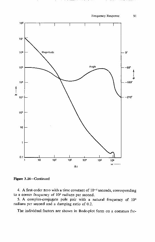

MIT OpenCourseWarehttpocwmitedu
RES6-010 Electronic Feedback SystemsSpring 2013
For information about citing these materials or our Terms of Use visit httpocwmiteduterms


![PDF[1.8MB] - Tokyo Chemical Industry Co., Ltd](https://img.pdfslide.us/doc/110x75/62073f2949d709492c2f747a/pdf18mb-tokyo-chemical-industry-co-ltd.jpg)