Linear regression relationships between NDVI, vegetation and rainfall in Etosha National Park, Namibia

Journal of Arid Environments (1999) 42: 235–260Article No. jare.1999.0505Available online at http://www.idealibrary.com on

0140-

Linear regression relationships between NDVI,vegetation and rainfall in Etosha National Park,

Namibia

W. P. du Plessis

Ministry of Environment & Tourism, Etosha Ecological Institute,P.O. Box 6, Okaukuejo, via Outjo, Namibia

(Received 28 July 1998, accepted 17 February 1999)

Estimations of 10-day interval green vegetation cover and biomass, 10-dayinterval cumulative rainfall, as well as annual rainfall are compared with 10-dayinterval and rainy season NDVI and MVC using linear regression analysis.Raw data were smoothed by averaging and removing dry season outliers.Results indicate that the ability of NDVI and MVC to predict green vegetationcover, cumulative rainfall and annual rainfall is poorer for raw data than foraveraged, outlier-removed data. It is recommended that the standard error ofthe raw data predictions are used to indicate the fundamental error in theserelationships, and that the equations of the averaged, outlier-removed data areused to indicate the fundamental strength of NDVI or MVC in predictingvegetation or rainfall. The practical use of integrated rainy season MVC imagesare discussed.

( 1999 Academic Press

Keywords: annual rainfall; cumulative rainfall; effective rainfall; greenvegetation cover and biomass; integrated rainy season MVC; NDVI; semi-aridsavannas; 10-day interval MVC

Introduction

The Etosha National Park (Etosha) is a large (22,915 km¨ 2) wildlife refuge in northernNamibia. Frequent monitoring of changes in rainfall, vegetation and animal movementsover the entire area is a momentous task using traditional ground-based methods, andcannot be maintained over a long period because of limited human and financialresources.

Satellite-derived NDVI (Normalized Difference Vegetation Index) and MVC(maximum value composite) are potentially very useful tools for the frequent monitor-ing of effective rainfall and green vegetation cover or biomass over large areas. TheNDVI and MVC may therefore be ideal tools for monitoring changes in vegetationduring the rainy season, which could contribute to more objective animal, water,vegetation and fire management in Etosha.

The NDVI is calculated from AVHRR (Advanced Very High ResolutionRadiometer) data from NOAA (National Oceanic and Atmospheric Administration)

1963/99/080235#26 $30.00/0 ( 1999 Academic Press

236 W. P. DU PLESSIS

polar orbiting satellites and is defined as:

NDVI"Channel 2!Channel 1Channel 2#Channel 1

(Eqn 1)

where Channel 1 and Channel 2 are the reflectance in the visible red (0)58 to 0)68 km)and near infrared channels (0)725 to 1)1 km), respectively. The NDVI is determined bythe degree of absorption by chlorophyll in the red wavelengths, which is proportional toleaf chlorophyll density, and by the reflectance of near infrared radiation, which isproportional to green leaf density (Tucker et al., 1985).

The maximum value composite (MVC) is calculated from a multi-temporal series ofgeometrically corrected NDVI images. On a pixel-by-pixel basis (picture element), eachNDVI value is examined, and only the highest value is retained for each pixel location(Holben, 1986). During the current study, MVC values were calculated from consecut-ive NDVI images over a 10-day period (10-day interval MVC).

Relationships between NDVI, rainfall and vegetation from the literature

The NDVI has been empirically shown to relate strongly to green vegetation cover andbiomass using ground-based studies involving spectral radiometers (Boutton & Tieszen,1983; Tucker et al., 1983; Huete & Jackson, 1987; Beck et al., 1990)

Many studies in the Sahel Zone (Tucker et al., 1985; Hielkema et al., 1986; Malo &Nicholson, 1990), Botswana (Prince & Tucker, 1986), East Africa (Boutton & Tieszen,1983; Davenport & Nicholson, 1993) and Tunisia (Kennedy, 1989) indicate meaning-ful direct relationships between NDVI derived from NOAA AVHRR satellites, rainfalland vegetation cover and biomass.

When predictions of rainfall or vegetation are compared for different NDVI-based studies, highly variable relationships are found (Hielkema et al., 1986; Groten,1991). These relationships vary in terms of their prediction strength (coefficient ofdetermination), amount of error (the standard error or standard deviation), slope andy-axis intercept.

There are many reasons for the variable relationships. The studies have been conduc-ted over many different soil and vegetation types, biomass, cover and greennessranges and at different times of the year. However, probably the most importantreason is that NDVI is seriously disturbed radiometrically due to complex radiativeinteractions between the atmosphere, sensor view angle and solar zenith angle (Van Dijket al., 1987). These factors reduce the reliability of the NDVI.

Many studies appear limited in that they do not incorporate the fundamental variabil-ity of NDVI when predicting vegetation and rainfall variables (Groten, 1991). Somestudies use statistical filters to smooth NDVI profiles (Van Dijk et al., 1987), but filteringdoes not remove the fundamental radiometric disturbance (Viovy et al., 1992). Also,many of these studies promote the use of NDVI as a sensitive tool for monitoring smallchanges in vegetation cover and biomass, although their results often indicate coef-ficient of determination values of less than 0)6 (Hellden & Eklundh, 1988; Nicholsonet al., 1990; Davenport & Nicholson, 1993).

Although NDVI is recognized as being limited in its use (Lillesand & Kiefer, 1994), itis still mostly used without appropriate consideration of the limitations. The implicationis that if NDVI is to be used as a prediction tool for rainfall and vegetation, thefundamental error in NDVI for predicting other variables such as total rainfall andvegetation cover needs to be incorporated in such predictions. Furthermore, theserelationships need to be calibrated for each climatic zone (arid, semi-arid, etc.) indifferent parts of the world. Relationships found in the semi-arid Sahel region are

RELATIONSHIPS BETWEEN NDVI, VEGETATION AND RAINFALL 237

not necessarily applicable to the semi-arid parts of Botswana (Farrar et al., 1994;Nicholson & Farrar, 1994) or East Africa (Nicholson et al., 1990).

Objectives

The objectives of this study are to: (i) introduce a pragmatic vegetation descriptionmethodology to relate to NDVI; (ii) provide empirical results of the relationshipsbetween NDVI, rainfall and vegetation for Etosha; (iii) indicate the high variabilityinherent in relationships between NDVI, rainfall and vegetation, and recommend howto incorporate this high variability to the NDVI-based predictions of vegetation andrainfall; and (iv) show examples of how integrated rainy season MVC images are used.

Data collection and analysis methods

Rainfall

Twenty raingauges of 50 cm length and 110 mm inner diameter were set up betweenSonderkop (gauge 1) and Halali (gauge 20), within 100 m of roads (Fig. 1). Ultraviolet-resistant PVC pipes were used as raingauges and sealed at the bottom with a PVC capand PVC cement. A plastic funnel was fitted to the inside on top. Fifteen millimeters ofmotor oil were added into each gauge to prevent evaporation of water, which was shownto be adequate for that purpose (Du Plessis, 1997). The gauges were placed approxim-ately 10 km apart, and were read every 10 days between the 21 September 1994 and the2 May 1995 (before the start of the rainy season until the start of the dry season). Gaugesthat were damaged or pushed over by animals were replaced during the following 10-dayinterval visit, and rainfall data (and corresponding vegetation descriptions and NDVIvalues) were discarded for that period. Data from raingauge number 5 were not includedin the analysis because of incorrect rainfall readings.

Ten-day interval rainfall data of the individual raingauges were extracted, and thecumulative rainfall calculated. The cumulative rainfall data of the different rain-gauges were then combined and compared with the appropriate study site’s vegetationvariables and satellite greenness indexes (NDVI and MVC values) for the correspond-ing period, using linear regression analysis. A study site was a 1 ha area around or closeto a raingauge.

Annual rainfall was measured at the 168 field raingauges distributed across Etosha,excluding pan areas. This represents a grid density of about 110 square km. Fieldraingauges, read once per year, are used primarily to identify areas that are to be burnt aspart of the burning strategy in Etosha (Du Plessis, 1997). The resulting annual rainfallmeasurements were compared in this study with the corresponding integrated rainyseason MVC values of the rainy season period between the 1 October and the 30 Aprilfor the years 1993/94, 1994/95 and 1995/96. Rainy season MVC pixels that werecontaminated by cloud, haze or dust were discarded, as well as rainfall data in caseswhere raingauges were found to be leaking.

Vegetation

Vegetation units surrounding each raingauge (study site) include a relativelyhomogenous area of approximately 2]2 km. The vegetation surrounding each studysite was inspected on the ground and Landsat TM satellite images were used to assess itshomogeneity. Largely different vegetation types were chosen as study sites, rangingfrom short grass plains to dense, high tree mopane savanna. Table 1 indicatesa structural description of the vegetation for the various sites. Figure 2 shows the

Fig

ure

1.Loc

atio

nof

the

stud

ysite

sin

Eto

sha,

Nam

ibia

.


Tab

le1.

Stru

ctur

alve

geta

tion

desc

ript

ion

ofth

e19

stud

ysite

sin

Eto

sha

Stru

ctur

alve

geta

tion

desc

ription

Stu

dysite

Hei

ght

cate

gory

Tota

lw

oody

crow

nnum

ber

and

vege

tation

type

cove

rde

nsity

Dom

inan

tsp

ecie

s

1Sh

rub

and

low

tree

sava

nna

Low

Col

opho

sper

mum

mop

ane

2Sh

rub

and

low

tree

sava

nna

Low

Col

opho

sper

mum

mop

ane

3Sh

rub

sava

nna

Low

Cat

ophr

acte

sal

exan

dri

4Sh

rub

and

low

tree

sava

nna

Med

ium

Col

opho

sper

mum

mop

ane

6Sh

rub

and

low

tree

sava

nna

Hig

hC

olop

hosp

erm

umm

opan

e7

Gra

ssla

ndan

dst

eppe

Ver

ylo

wA

nnual

gras

ses

and

Mon

echm

age

nist

ifoliu

m8

Shru

ban

dtr

eesa

vann

aLow

Col

opho

sper

mum

mop

ane

and

Aca

cia

nebr

owni

i9

Hig

htr

eesa

vann

aLow

Mor

inga

oval

ifolia

and

Col

opho

sper

mum

mop

ane

10G

rass

land

and

Step

peLow

Ann

ual

gras

ses

and

¸eu

cosp

haer

aba

ines

ii11

Gra

ssla

ndan

dst

eppe

Low

Ann

ual

gras

ses

and

¸eu

cosp

haer

aba

ines

ii12

Gra

ssla

ndan

dst

eppe

Ver

ylo

wto

low

Ann

ual

gras

ses

and

¸eu

cosp

haer

aba

ines

ii13

Shru

ban

dlo

wtr

eesa

vann

aLow

Col

opho

sper

mum

mop

ane

and

Aca

cia

mel

lifer

a14

Low

and

high

tree

sava

nna

Med

ium

Col

opho

sper

mum

mop

ane

and

¹er

min

alia

prun

ioid

es15

Gra

ssla

ndan

dst

eppe

Low

¸eu

cosp

haer

aba

ines

ii,Sal

sola

tube

rcul

ata,

and

Pet

alid

ium

engl

eran

um16

Shru

bsa

vann

aLow

Aca

cia

nebr

owni

i17

Hig

htr

eesa

vanna

Med

ium

Col

opho

sper

mum

mop

ane

18G

rass

land

and

step

peLow

¸eu

cosp

haer

aba

ines

iian

dC

yath

ula

here

roen

sis

19Pan's

edge

gras

slan

dV

ery

low

Mos

tly

pere

nnia

lgr

asse

san

dso

me

dw

arfsh

rubs

20H

igh

tree

and

shru

bsa

vanna

Med

ium

Col

opho

sper

mum

mop

ane,

Cat

ophr

acte

sal

exan

drian

dA

caci

are,ci

ens


Fig

ure

2.D

iagr

amofco

ver

and

hei

ghtcl

asse

suse

din

the

stru

ctura

ldes

crip

tion

ofve

geta

tion

.



decision tree used for the structural vegetation description. The crown cover is related tothe canopy-to-gap ratio of the woody component, which is defined as the mean gapbetween canopies divided by the canopy diameter (Wakler & Cropper, 1988).

Different vegetation variables were described at 10-day intervals and colourphotos were taken monthly showing the entire study site. The vegetation variablesdescribed were: (i) grasses and herbs; species composition, standing crop (biomass),total cover, greenness, green cover (cover of the green component of grasses); (ii) dwarfshrubs; species composition, total cover, percentage leaves, leaf greenness, green cover(cover of the green component of dwarf shrubs); (iii) shrub and trees; species composi-tion, total cover, percentage leaves, leaf greenness, green cover (cover of the greencomponent of shrub and trees); (iv) total vegetation cover of study site; and (v) totalgreen vegetation cover of study site (cover of the green component of the vegetation).

Most of the above vegetation variables were only described to aid in the estimation ofthe total vegetation cover and total green vegetation cover. The variables grass greenstanding crop, grass green cover and total green vegetation cover were found to be mostimportant in their relationship to NDVI and rainfall.

Grass green standing crop was estimated. These estimations were based on measure-ments where a disc pasture meter had been calibrated in Etosha to estimate totalgrass standing crop as part of the burning strategy (Du Plessis, 1997). Total grassstanding crop was firstly estimated, and then the green grass standing crop componentwas estimated separately. Classes used were: extremely low (4286 kg ha!1), very low(287}628 kg ha!1), low (629}1235 kg ha!1), medium (1236}2032 kg ha!1),high (2033}3020 kg ha!1), very high (3021}4197 kg ha!1) and extremely high('4197 kg ha!1).

Grass green cover was also estimated. Green cover describes how much of the soil wascovered by green grasses and herbs alone. Percentage classes used were: extremely low(0}1%), very low (1}5%), low (5}25%), medium (25}50%), high (50}75%) and veryhigh ('75%).

The total green vegetation cover (of grasses and herbs, dwarf shrubs, and shrub andtrees) for each site was estimated, and this estimation was refined from detaileddescriptions for each site and each vegetation stratum, and from the informationcontained in the photos taken of the entire site. Percentage classes used were: extremelylow (0}1%), very low (1}5%), low (5}25%), medium (25}50%), high (50}75%) andvery high ('75%).

The above descriptions of extremely low to very high cover and standing crop wereclassed to values of 1 to 6 for analysis purposes. Table 2 show how these values relate todescriptions and percentage ranges of cover and standing crop used.

The estimation of actual percentage values of the above vegetation variables in thefield were found to be inaccurate and inconsistent. Therefore, the above classificationsystem with broad, well-defined percentage ranges (class 1 to 6) was used instead.

Table 2. Descriptions of extremely low to very high percentage cover and standingcrop ranges related to analysis classes 1 to 6

Class Description Percentage cover Standing crop

1 Extremely low coveror standing crop 0}1% 4286 kg ha!1

2 Very low 1}5% 287}628 kg ha!1

3 Low 5}25% 629}1235 kg ha!1

4 Medium 25}50% 1236}2032 kg ha!1

5 High 50}75% 2033}3020 kg ha!1

6 Very high 75}100% 3021}4197 kg ha!1


NDVI and MVC

The NDVI data for Namibia obtained from NOAA 11 were captured at the EtoshaEcological Institute and processed using a LARST (Local Application of RemoteSensing Technology) system (Stephenson, 1991). Standard procedures were followedfor geometrical and atmospheric corrections (Lillesand & Kiefer, 1994). Furthermore,NOAA images were geometrically corrected to the nearest 2 km using the Etosha Pan asa co-ordination reference. The Etosha Pan, a barren area with no vegetation and mostlyno water, has a distinct outline that is clearly visible using different spectral channelsfrom NOAA images.

For each study site, the NDVI value was extracted from one pixel corresponding mostclosely to the site’s ground co-ordinates using Idrisi for Windows GIS software. Duringpreliminary analysis the average NDVI value of nine pixels surrounding a study sitecorresponded closely to the NDVI value of the one pixel closest to the study site. Theaverage values from the nine pixels were therefore ignored during final comparisons ofNDVI with vegetation and rainfall. The NDVI image used corresponded most closely tothe date at which the rainfall was measured and the vegetation was described for eachsite. The 10-day interval MVC value of each site was additionally calculated for the same10-day interval as rainfall measurements and vegetation descriptions. The NDVI andMVC values were evaluated using the Etosha Pan as a calibration target.

The NDVI and MVC values that were obviously contaminated by atmospheric noise(clouds, water vapour, haze and especially dust) or satellite error were not included inthe analysis. Strong contamination was detected by examining a specific NDVI or MVCimage against consecutive and preceding images, and discarding a study site’s NDVI orMVC values if the values appeared to be generally much higher or lower than the valuesaround each site for preceding or consecutive images. Great care was taken during thisprocess for the period at the beginning and end of the rainy season, because substantialchanges could be expected. Images were also discarded when many pixels had extremelyhigh values in the dry period. This error was attributed to signal noise resulting frompoor reception, but did not occur too often. Furthermore, images that were highlyaffected by clouds were also masked using standard cloud-masking techniques(Stephenson, 1991) and discarded from the analysis. Rainfall measurements and vegeta-tion descriptions of corresponding dates where NDVI and MVC values were discarded,were also left out of the final analysis.

Integrated rainy season MVC were calculated by extracting the maximum NDVIvalue of multi-temporal NDVI images over the rainy season period between the1 October and 30 April for the years 1993/94, 1994/95 and 1995/96.

The NDVI, MVC and rainy season MVC values, as well as rainfall and vegetationvalues (ranked 1 to 6) were compared with each other using linear regression analysis.Preliminary logarithmic regression analysis produced comparable coefficient ofdetermination results to linear regression analysis, and the latter was preferred for ease ofuse and interpretation.

Results and discussion

NDVI vs. vegetation

Figure 3 is a comparison of total green vegetation cover with NDVI of the raw data of all19 study sites combined. The data are sorted by date. A polynomial trendline of the fifthorder is fitted to each of the data sets.

Two aspects are apparent. The first is the high variability in the vegetation and NDVIdata, which reflects the differences in green vegetation cover between the dif-ferent study sites for different dates. Until the start of the main rainy season at the

Figure 3. Line plot comparing NDVI with total green vegetation cover of raw data. (h) Totalgreen vegetation cover; (r) NDVI; (**) polynomial trendline (NDVI); ( ) polynomialtrendline (total green vegetation cover).


beginning of February 1995, largely varying total green vegetation cover values wererecorded, but the NDVI seemed to stay relatively low. During the rainy season, bothvegetation and NDVI values increased, and then decreased towards the end of the rainyseason (by the middle of April 1995). The changes in total green vegetation cover areconsidered to be much closer to the actual situation observed in the field than indicatedby the changes in NDVI. (This is because vegetation classes have relatively large ranges(most are 25% in width), and the chance of correctly describing the total greenvegetation cover value and trend is seen as being much higher than the NDVI valuereflecting the correct trend.) This is due to the much smaller increments in NDVIcompared to vegetation descriptions in this study, which may for example indicatea slight to strong decreasing trend when in fact the total green vegetation cover stayed thesame or increased. This is attributed to atmospheric noise, sensor view angle and solarzenith angle effects having a negative influence on NDVI’s reliability.

The second aspect of Fig. 3 is that the two polynomial trendlines show a very highcorrespondence. Polynomial trendlines are not necessarily the most appropriate smooth-ing technique (Van Dijk et al., 1987) because they cannot reflect small changes in thedata, but it is clear that the basic trend of the two data sets are very similar. This study ismostly concerned with the basic trend between the different variables.

Figure 4 is a linear regression line plot of raw data of NDVI predicting total greenvegetation cover. The large variability is again clearly apparent. The low coefficientof determination value (0)5166) and high standard error of the y-axis predicted by thex-axis (1)05) indicate a poor relationship, which cannot be relied upon in any prediction(even though many papers indicate similar poor values as ‘meaningful’ and ‘sensitive’).

To reveal the strong relationship of the underlying trend indicated by the polynomialtrendlines in Fig. 3, the data sets were smoothed by averaging. Ranges of 20 consecut-ively paired values of total green vegetation cover and NDVI were smoothed bycalculating the arithmetic mean of these pairs. It was considered inappropriate to usemore refined trend and smoothing techniques such as ARIMA, exponential smoothing


or 4253H moving average smoothing, because the aim was to bring out the underlyingstrong relationship between these variables, and not to retain smaller variations that arenecessary for detailed interpretation of changes in the seasonal time series (Van Dijket al., 1987). Figure 5 is a comparison of total green vegetation cover with NDVI of the

Figure 5. Linear regression analysis comparing NDVI with total green vegetation cover ofaveraged data. (r) Total green vegetation cover; (**) linear (total green vegetation cover).

Figure 4. Linear regression analysis comparing NDVI with total green vegetation cover of rawdata. (r) Total green vegetation cover; (**) linear (total green vegetation cover).

Figure 6. Linear regression analysis comparing NDVI with total green vegetation cover ofaveraged, dry season outlier-removed data. (r) Total green vegetation cover; (**) linear (totalgreen vegetation cover).


averaged data of all 19 study sites combined using linear regression analysis. Thecoefficient of determination value of 0)8584 indicates a much stronger underlyingrelationship than the raw data’s coefficient of determination value of only 0)5166.The standard error of the y-axis predicted by the x-axis is also much lower at 0)44.

The NDVI has been shown in the literature to relate strongly to changes in greenvegetation cover or biomass, but not to dry vegetation or vegetation with a low greencover (Boutton & Tieszen, 1983; Huete & Jackson, 1987; Beck et al., 1990; Verstraete& Pinty, 1991). The raw and averaged data sets in this study incorporated data from theperiod before and after the rainy season. When paired outliers were removed from theaveraged data set (Fig. 6), the relationship improved even further to a coefficient ofdetermination value of 0)9129 and a standard error of the y-axis predicted by the x-axisof 0)31 using linear regression analysis. These values are interpreted as indicating anunderlying strong relationship between NDVI and total green vegetation cover.

NDVI vs. MVC

Ten-day interval MVC values were also calculated for each of the study sites.Figure 7 indicates the close correspondence between NDVI and MVC predicting totalgreen vegetation cover after dry season outliers were removed from the averaged datapairs. Table 3 shows some statistics and the equations of the independent variable(x-axis) predicting the dependent variable (y-axis) for the various variables of raw andaveraged data. Ten-day interval MVC has the advantage over NDVI that more atmo-spheric noise is removed (Holben, 1986). Ten-day interval MVC images are routinelyproduced and archived at the Etosha Ecological Institute, and is the standard productused to produce integrated rainy season MVC images. Therefore, 10-day interval MVCwere related to total green vegetation cover and cumulative rainfall, and the equationsthereof used rather than equations produced by single image NDVI values.

Figure 7. Comparison of linear regression equations plotted for total green vegetation coverpredicted by NDVI (*) and by MVC ( ) for averaged, dry season outlier-removed data.


MVC vs. vegetation vs. rainfall

The NDVI or MVC and vegetation was found to relate much more strongly tocumulative rainfall than to individual 10-day interval rainfall. This is because of a timelag in NDVI and vegetation response to rainfall (Hellden & Eklundh, 1988; Kennedy,1989; Malo & Nicholson, 1990; Groten, 1991; Davenport & Nicholson, 1993; Nichol-son & Farrar, 1994), and because rainfall in Etosha is spatially and temporally highlyvariable (Engert, 1992). Small amounts of rain (less than 20 mm) do not result ina significant increase in green vegetation cover, especially if consecutive rainfall eventsare more than about 5 days apart (pers. obs.). Cumulative rainfall, and not individualdaily rainfall, was therefore used in the comparison of MVC and vegetation.

Figure 8 shows the direct relationship between the 10-day interval MVC values on thex-axis predicting total green vegetation cover (on y-axis 1), and cumulative rainfall (ony-axis 2), using the equations from the averaged data with the dry season outliersremoved. Table 4 shows some statistics and the equations of the independent variable(x-axis) predicting the dependent variable (y-axis) for the various variables of raw andaveraged data. Cumulative rainfall was averaged in a similar way to MVC and total greenvegetation cover, and paired dry season outliers were removed. These relationships cantherefore be used to estimate two unknown variables if one is known or can be estimated.

It is recommended that the standard error of the raw data sets is used to calculate theamount of variability below or above the y-axis value predicted by the x-axis variable,and not to use the standard error of the averaged (smoothed) data for that purpose. Thereason is that the raw data show the actual amount of error in the data, which is in factnot removed by averaging (Viovy et al., 1992). Averaging just brings out the underlyingstrong trend between these variables and produces a more reliable equation for predic-tions of one or more variables by another.

The equations in Table 4 that were used to draw Fig. 8 produce for example an MVCvalue of 0)15 during the rainy season which predicts a total green vegetation cover ofclass 4)1, and the standard error of the y-axis predicted by the x-axis of the raw data is$0)96. An MVC of 0)15 predicts a cumulative rainfall of 276)68 mm with the standarderror of the raw data being $102)89 mm.

Tab

le3.

¸in

ear

regr

ession

equa

tion

san

dst

atistics

ofM<

Cco

mpa

red

with

ND<

Ipr

edic

ting

tota

lgr

een

cove

r.R

2 "co

e.ci

ent

ofde

term

inat

ion;

SE>

X"

stan

dard

erro

rof

the

y-ax

is(in

depe

nden

tva

riab

le)pr

edic

ted

byth

ex-a

xis

(dep

ende

ntva

riab

le);

N"

num

ber

ofob

serv

atio

ns.¹

hepr

obab

ility

valu

eis

(0)

001

for

allre

lation

ship

s

Inde

pend

ent

variab

leD

epen

dent

variab

leLin

ear

regr

ession

Dat

aty

pe(x

-axi

s)(y

-axi

s)eq

uation

R2

SEY

XN

Raw

MV

Cto

talgr

een

vege

tation

cove

ry"

(12)

838)

x#

1)86

240)

5988

0)96

266

Raw

tota

lgr

een

vege

tation

cove

rM

VC

y"(0)0

466)

x!0)

0601

0)59

880)

0626

6A

vera

ged

and

outlie

rsre

move

dM

VC

tota

lgr

een

vege

tation

cove

ry"

(14)

103)

x#1)

9562

0)92

391)

0110

Ave

rage

dan

dou

tlie

rsre

move

dto

talgr

een

vege

tation

cove

rM

VC

y"(0)0

655)

x!0)

1231

0)92

390)

0210

Raw

ND

VI

tota

lgr

een

vege

tation

cove

ry"

(14)

139)

x#1)

9534

0)51

661)

0520

4R

awto

talgr

een

vege

tation

cove

rN

DV

Iy"

(0)0

365)

x#0)

0426

0)51

660)

0520

4A

vera

ged

and

outlie

rsre

move

dN

DV

Ito

talgr

een

vege

tation

cove

ry"

(16)

412)

x#1)

7886

0)91

290)

317

Ave

rage

dan

dou

tlie

rsre

move

dto

talgr

een

vege

tation

cove

rN

DV

Iy"

(0)0

556)

x!0)

0948

0)91

290)

027


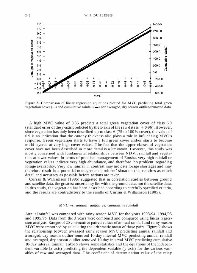
Figure 8. Comparison of linear regression equations plotted for MVC predicting total greenvegetation cover (*) and cumulative rainfall ( ), for averaged, dry season outlier-removed data.


A high MVC value of 0)35 predicts a total green vegetation cover of class 6)9(standard error of the y-axis predicted by the x-axis of the raw data is $0)96). However,since vegetation has only been described up to class 6 (75 to 100% cover), the value of6)9 is an indication that the canopy thickness also plays a role in influencing MVC’sresponse. Green vegetation starts to have a full green cover and/or starts to becomemulti-layered at very high cover values. The fact that the upper classes of vegetationcover have not been described in more detail is a limitation. However, this study wasmostly concerned with fundamental relationships between NDVI, rainfall and vegeta-tion at lower values. In terms of practical management of Etosha, very high rainfall orvegetation values indicate very high abundance, and therefore ‘no problem’ regardingforage availability. Very low rainfall in contrast may indicate forage shortages and maytherefore result in a potential management ‘problem’ situation that requires as muchdetail and accuracy as possible before actions are taken.

Curran & Williamson (1985) suggested that in correlation studies between groundand satellite data, the greatest uncertainty lies with the ground data, not the satellite data.In this study, the vegetation has been described according to carefully specified criteria,and the results are contradictory to the results of Curran & Williamson (1985).

MVC vs. annual rainfall vs. cumulative rainfall

Annual rainfall was compared with rainy season MVC for the years 1993/94, 1994/95and 1995/96. Data from the 3 years were combined and compared using linear regres-sion analysis. Ranges of 20 consecutive paired values of annual rainfall and rainy seasonMVC were smoothed by calculating the arithmetic mean of these pairs. Figure 9 showsthe relationship between averaged rainy season MVC predicting annual rainfall andaveraged, dry season outlier-removed 10-day interval MVC predicting annual rainfalland averaged, dry season outlier-removed 10-day interval MVC predicting cumulative10-day interval rainfall. Table 5 shows some statistics and the equations of the indepen-dent variable (x-axis) predicting the dependent variable (y-axis) for the various vari-ables of raw and averaged data. The coefficient of determination value of the rainy

Tab

le4.

¸in

ear

regr

ession

equa

tion

san

dst

atistics

ofM<

Cco

mpa

red

with

tota

lgr

een

cove

ran

dcu

mul

ativ

era

infa

ll.R

2 "co

e.ci

ent

ofde

term

inat

ion;

SE>

X"

stan

dard

erro

rof

the

y-ax

is(in

depe

nden

tva

riab

le)pr

edic

ted

byth

ex-a

xis

(dep

ende

ntva

riab

le);

N"

num

ber

ofob

serv

atio

ns.¹

hepr

obab

ility

valu

eis

(0)

001

for

allre

lation

ship

s

Inde

pend

ent

variab

leD

epen

dent

variab

leLin

ear

regr

ession

Dat

aty

pe

(x-a

xis)

(y-a

xis)

equa

tion

R2

SEY

XN

Raw

tota

lgr

een

vege

tation

cove

rcu

mul

ativ

era

infa

lly"

(55)

543)

x#0)

2914

0)33

7311

8)13

266

Raw

cum

ula

tive

rain

fall

tota

lgr

een

vege

tation

cove

ry"

(0)0

061)

x#1)

7995

0)33

731)

2426

6R

awM

VC

tota

lgr

een

vege

tation

cove

ry"

(12)

838)

x#1)

8624

0)59

880)

9626

6R

awto

talgr

een

vege

tation

cove

rM

VC

y"(0)0

466)

x!0)

0601

0)59

880)

0626

6R

awM

VC

cum

ulat

ive

rain

fall

y"(1

118)

8)x#

76)6

970)

4973

102)

8926

6R

awcu

mul

ativ

era

infa

llM

VC

y"(0)0

004)

x!0)

0006

0)49

730)

0726

6

Ave

rage

dan

dou

tlie

rsre

mov

edto

talgr

een

vege

tation

cove

rcu

mul

ativ

era

infa

lly"

(120

)47)

x!21

7)42

0)95

5227)2

110

Ave

rage

dan

dou

tlie

rsre

mov

edcu

mul

ativ

era

infa

llto

talgr

een

vege

tation

cove

ry"

(0)0

079)

x#1)

8533

0)95

520)

2410

Ave

rage

dan

doutlie

rsre

move

dM

VC

tota

lgr

een

vege

tation

cove

ry"

(14)

103)

x#1)

9562

0)92

391)

0110

Ave

rage

dan

dou

tlie

rsre

mov

edto

talgr

een

vege

tation

cove

rM

VC

y"(0)0

655)

x!0)

1231

0)92

390)

0210

Ave

rage

dan

dou

tlie

rsre

mov

edM

VC

cum

ulat

ive

rain

fall

y"(1

801)

4)x#

6)47

360)

9626

27)2

112

Ave

rage

dan

dou

tlie

rsre

mov

edcu

mul

ativ

era

infa

llM

VC

y"(0)0

005)

x!0)

0008

0)96

260)

0212


Figure 9. Comparison of linear regression equations of cumulative 10-day interval rainfallpredicted by 10-day interval MVC (**) and annual rainfall predicted by rainy season MVC( ), for averaged data.


season MVC equation predicting annual rainfall is 0)8374 (of averaged data), and thestandard error of the y-axis predicted by the x-axis of the raw data’s equation is 68)62.The coefficient of determination value of the 10-day interval MVC equationpredicting cumulative 10-day interval rainfall is 0)9626, and the standard error of they-axis predicted by the x-axis of the raw data’s equation is 102)89.

The equation of rainfall predicted by 10-day interval MVC and by rainy season MVCproduced significantly different results (Fig. 9). The cumulative 10-day intervalrainfall prediction has a much steeper slope than the annual rainfall prediction. Theexplanation is that 10-day interval vegetation response is more closely related tocumulative 10-day interval rainfall than to annual rainfall. Cumulative rainfall to a cer-tain degree represents effective rainfall (efficient use of rain) in terms ofvegetation development. Vegetation development tracks cumulative rainfall over therainy season, but not daily rainfall, and cumulative rainfall therefore relates better toMVC than normal rainfall does.

Annual rainfall, in contrast to cumulative 10-day interval rainfall, is the total dailyrainfall added up over the entire season without incorporating related vegetation re-sponse in the same manner as cumulative rainfall. The total annual rainfall amount ismostly not effective in terms of vegetation growth. For example, a rainy season mayhave periods with very little rainfall and with no vegetation reaction, as well as periodswith very high rainfall over a short period with also relatively poor vegetation responsebecause of water logging or high infiltration, runoff and evaporation. Under thesecircumstances, annual rainfall cannot reflect vegetation growth accurately, and thereforeit also does not reflect MVC’s response to rainfall.

Ten-day interval MVC is closely lined with 10-day interval vegetation response andtherefore with cumulative 10-day interval rainfall. Rainy season MVC, on the otherhand, is showing effective rainfall for an entire season, which is not represented bythe annual rainfall as explained above. Therefore, rainy season MVC is of much morevalue than total annual rainfall. For illustration, in Fig. 9, the extremely high MVC valueof 0)502 predicts an annual rainfall of 426)90 mm (the standard error of the y-axispredicted by the x-axis of the raw data’s equation is $68)62), whereas the same MVCvalue predicts cumulative 10-day interval rainfall of 910)83 mm (the standard error of

Tab

le5.

¸in

ear

regr

ession

equa

tion

san

dst

atistics

of10

-day

inte

rval

M<

Cco

mpa

red

with

cum

ulat

ive

rain

fall,

rain

yse

ason

M<

Cco

mpa

red

with

annu

alra

infa

ll,an

dra

iny

seas

onM<

Cof

10-d

ayin

terv

alra

inga

uges

com

pare

dwith

annu

alra

infa

llof

10-d

ayin

terv

alra

ingu

ages

.R

2 "co

e.ci

ent

ofde

term

inat

ion;

SE>

X"

stan

dard

erro

rof

the

y-ax

is(in

depe

nden

tva

riab

le)

pred

icte

dby

the

x-a

xis

(dep

ende

ntva

riab

le);

N"

num

ber

ofob

serv

atio

ns.¹

hepr

obab

ility

valu

eis

(0)

001

for

allre

lation

ship

s

Inde

pend

ent

variab

leD

epen

dent

variab

leLin

ear

regr

ession

Dat

aty

pe(x

-axi

s)(y

-axi

s)eq

uat

ion

R2

SEY

XN

Raw

10-d

ayin

terv

alM

VC

cum

ulat

ive

rain

fall

y"(1

118)

8)x#

76)6

970)

4973

102)

8926

6R

awra

iny

seas

onM

VC

annu

alra

infa

lly"

(584

)65)

x#13

7)36

0)30

2668)6

228

4

Ave

rage

dan

dou

tlie

rsre

mov

ed10

-day

inte

rval

MV

Ccu

mul

ativ

era

infa

lly"

(180

1)4)

x#6)

4736

0)96

2627)2

112

Ave

rage

dra

iny

seas

onM

VC

annu

alra

infa

lly"

(570

)39)

x#14

0)55

0)83

7420)3

714

Raw

rain

yse

ason

MV

Cat

Ann

ual

rain

fall

of

y"(5

82)0

9)x#

32)2

20)

7369

32)5

719

10-d

ayin

terv

alra

inga

uge

s10

-day

inte

rval

rain

gauge

s

Raw

Ann

ual

rain

fall

of

Rai

nyse

ason

MV

Cat

y"(0)0

013)

x#0)

0127

0)73

690)

0519

10-d

ayin

terv

alra

inga

uge

s10

-day

inte

rval

rain

gauge

s



the y-axis predicted by the x-axis of the raw data’s equation is $102)89), more thandouble the total annual rainfall, and indicates the potential effective rainfall (but nottrue rainfall).

To illustrate the point further, if the total annual rainfall at a specific location is, forexample, 500 mm, the effective rainfall in terms of plant growth (especially forannual plants) is less than 250 mm ((50%) in a semi-arid area such as Etosha. Thisrelationship may vary between years, depending on how effective the rainfallactually was, but the rainy season MVC values can provide a good representation ofeffective rainfall over a rainy season period.

Figure 10 shows the relationship between annual rainfall of the 168 annual raingaugesand the annual rainfall of the 10-day interval raingauges as predicted by the related rainyseason MVC’s. The trend between the two predicted rainfall calculations is nearlyidentical, but the annual rainfall of the 10-day interval raingauges is even lower than theannual rainfall of the 168 annually-read raingauges. This indicates that the rainfall of the1994/95 rainy season was even less effective than when using the average betweenthe rainy seasons of 1993/94 to 1995/96. Table 5 includes the linear regression equa-tions of the rainy season MVC at 10-day interval raingauges vs. annual rainfall of 10-dayinterval raingauges.

Different vegetation variables compared (and remarks on relationships with NDVI)

Of the various vegetation variables recorded for the different components in thevegetation (see ‘Methods’), total green vegetation cover, grass green cover and grassgreen standing crop correlated strongest to NDVI or MVC. Of these, grass green covermostly correlated the strongest with NDVI or MVC (unpublished data). Dwarf shrubsgreen cover correlated very poorly to NDVI or MVC because of their predominantlyvery low or low cover (usually less than 5% cover). Shrubs and trees at most of the studysites also had a low cover. The most dominant woody vegetation type in Etosha ismopane shrubs and trees. These developed most of their green leaves ('60%) beforeany rain fell, and stayed in leaf until after the rainy season, resulting in poor relationshipsbetween NDVI and shrub and tree green cover.

Figure 10. Comparison of linear regression equations plotted for annual rainfall of annualraingauges predicted by rainy season MVC at annual raingauges (*), and annual rainfall of10-day interval raingauges predicted by rainy season MVC at 10-day interval raingauges ( ).


Figure 11 shows the plotted equations of grass green standing crop predicting grassgreen cover and total green vegetation cover where the raw data have been averaged ina similar way as described earlier. No outliers needed to be removed because dry seasondescriptions were just as accurate as rainy season descriptions and were not influencedby noise in the same way that NDVI or MVC values are. Table 6 shows some statisticsand the equations of the independent variable (x-axis) predicting the dependent variable(y-axis) for the various variables of the raw and averaged data. The standard error of they-axis predicted by the x-axis of the raw data should be used to indicate the error in thepredictive data. Table 6 also indicates that grass green standing crop relates much betterto grass green cover than to total green vegetation cover (according to raw data’scoefficient of determinant values), as expected.

Figure 11 further indicates that a grass green standing crop of, for example, class 3)0predicts a grass green cover of 3)8, and a total green vegetation cover of 5)2. If the grassgreen standing crop is 6)0, the grass green cover predicted is 7)9, and the total greenvegetation cover predicted is 10)1. As indicated before, in the description of differ-ent vegetation variables, only class 1 to 6 were allocated, with 6 representing a very highcover or very high standing crop (75 to 100% cover or 3021 to 4197 kg ha!1 standingcrop). Predictive values of higher than 6)0 suggest higher than 100% cover, which is notpossible and indicates that the density of the canopy also plays a role in the relationshipsbetween vegetation cover, biomass and NDVI. Therefore, when the green vegetationcover is high or very high, it also starts to become multi-layered. Furthermore, relation-ships between green vegetation cover and NDVI at higher values were found to departfrom linearity and became exponential because vegetation reaches maximum photosyn-thetic capacity even though growth may continue (Malo & Nicholson, 1990).

The use of rainy season MVC

Figure 12(a, b) shows images of the rainy season MVC’s of Etosha for the years1996/97 and 1997/98, respectively. The rainy season of 1996/97 was a year with

Figure 11. Comparison of linear regression equations plotted for grass green standing croppredicting grass green cover (m) and total green vegetation cover (j) for averaged, dry seasonoutlier-removed data.

Tab

le6.

¸in

earre

gres

sion

equa

tion

san

dstat

istics

ofgr

assgr

een

stan

ding

crop

com

pare

dwith

gras

sgr

een

cove

ran

dto

talg

reen

vege

tation

cove

r.R

2 "co

e.ci

entof

dete

rmin

atio

n;SE>

X"

stan

dard

erro

rof

the

y-ax

is(in

depe

nden

tva

riab

le)p

redi

cted

byth

ex-a

xis

(dep

ende

ntva

riab

le);

N"

num

ber

ofob

serv

atio

ns.¹

hepr

obab

ility

valu

eis

(0)

001

for

allre

lation

ship

s

Inde

pend

ent

variab

leD

epen

dent

variab

leD

ata

type

(x-a

xis)

(y-a

xis)

Lin

ear

regr

ession

equat

ion

R2

SEY

XN

Raw

gras

sgr

een

stan

ding

crop

gras

sgr

een

cove

ry"

(1)1

781)

x!0)

0673

0)82

850)

4720

4R

awgr

ass

gree

nco

ver

gras

sgr

een

stan

ding

crop

y"(0)7

033)

x#0)

3104

0)82

850)

3620

4R

awgr

ass

gree

nst

andi

ngcr

opto

talgr

een

vege

tation

cove

ry"

(1)2

306)

x#0)

9061

0)50

801)

0620

4R

awto

talgr

een

vege

tation

cove

rgr

ass

gree

nst

andi

ngcr

opy"

(0)4

128)

x#0)

3809

0)50

800)

6120

4R

awgr

ass

gree

nco

ver

tota

lgr

een

vege

tation

cove

ry"

(0)9

647)

x#1)

1153

0)52

301)

0420

4R

awto

talgr

een

vege

tation

cove

rgr

ass

gree

nco

ver

y"(0)5

421)

x#0)

2256

0)52

300)

7820

4

Ave

rage

dgr

ass

gree

nst

andi

ngcr

opgr

ass

gree

nco

ver

y"(1)3

85)x

!0)

378

0)96

050)

1910

Ave

rage

dgr

ass

gree

nco

ver

gras

sgr

een

stan

ding

crop

y"(0)6

935)

x#0)

322

0)96

050)

1310

Ave

rage

dgr

ass

gree

nst

andi

ngcr

opto

talgr

een

vege

tation

cove

ry"

(1)6

445)

x#0)

273

0)91

020)

3510

Ave

rage

dto

talgr

een

vege

tation

cove

rgr

ass

gree

nst

andi

ngcr

opy"

(0)5

535)

x!0)

0152

0)91

020)

2010

Ave

rage

dgr

ass

gree

nco

ver

tota

lgr

een

vege

tation

cove

ry"

(1)1

696)

x#0)

7522

0)91

960)

3310

Ave

rage

dto

talgr

een

vege

tation

cove

rgr

ass

gree

nco

ver

y"(0)7

863)

x!0)

4533

0)91

960)

2710



above-average rainfall in Etosha, and the wettest year since 1978. The rainy season of1997/98 was a year with below-average rainfall over most of Etosha.

The NDVI is considered to be of little or no use in the critical dry season period. Therainy season MVC is therefore used to predict the maximum potential available biomassfor the following dry season, which may be as long as 9 months in Etosha (May toJanuary). The rainy season MVC values were classed into relatively broad qualitativeclasses based on field observations and quantitative results from this study. A low rainyseason MVC value, for example, is therefore used to indicate low levels of greenvegetation biomass, which may be interpreted as the result of low effective rainfall,which results in low forage availability for large grazers. A low rainy season MVC valuemay also indicate that an area has a low carrying capacity for large grazers, or an areamay have a low risk of fires spreading uncontrolled over a large area.

It is preferable to use the qualitative rainy season MVC classes (extremely low to veryhigh) in the decision-making process of national park management over trying to usemore complex quantitative parameters that are nearly impossible to define. For example,carrying capacity, which is an extremely variable concept dependent on many dynamicfactors, is very difficult to assess accurately and use successfully in large naturalsavannas. Therefore, qualitative rainy season MVC classes are preferred above quantit-ative carrying capacity values. Qualitative rainy season MVC classes are used in thefollowing manner. Low biomass availability derived from rainy season MVC valuesmay, for example, indicate high risk of forage shortage in the dry season for largergrazers, which may demand high levels of involvement from national park staff. Onthe other hand, very high biomass availability derived from rainy season MVC valuesmay indicate very low risk of forage shortage in the dry season for larger grazers, whichmeans no demand on the time of national park staff to provide water in areas withmore abundant forage to attract wildlife. However, such an abundant biomass situationmay demand high levels of involvement in that tracks and roads need to be graded intime to be able to control natural or accidental fires from spreading over too large areasin the following dry season.

Table 7 shows the categorization of the rainy season MVC images of Fig. 12(a, b) intoMVC and green vegetation biomass descriptive classes. These classes were definedusing the Etosha Pan as a calibration target for indicating bare ground, and dividing theMVC values above that into 15 equal digital number ranges, except for the last classwhich has a range of 33 digital numbers. Table 7 also includes values of MVC predi-cting total green cover using the appropriate equation from Table 4. The total greencover predicted by MVC (Fig. 8; Table 4) is about two to three classes higher than thegreen vegetation biomass indicated by the rainy season MVC images of Fig. 12(a, b)(Table 7).

Descriptions of total green vegetation cover are not directly related to green biomassor green standing crop (see ‘different vegetation variables compared’). Also, MVC(or NDVI) relates very poorly to total green vegetation cover values of lower than about30% (at the lower level of class 4 used in this study). The MVC values between digitalnumber’s !0)13 and 0)10 (bare ground) were often related to field descriptions of totalgreen cover values between 2 and 4 (very low to moderate total green vegetation cover).Therefore, predictions of total green vegetation cover by MVC produced about two tothree classes higher estimations than that of green vegetation biomass.

Another factor to consider in the use of the rainy season MVC is that vegetationbiomass is constantly being reduced as the dry season progresses. Field observationsshowed that just after the rainy season the grass biomass may for example be very high(class 6), but by the end of the dry season the grass biomass may have been reduced tomoderate (class 4) or even low (class 3) values in areas with high grazing pressure.Therefore, with low or very low rainy season MVC values, a reduction in biomass can beexpected towards the end of the dry season to levels of extremely low or even no biomassleft.


Fig

ure

12.

Rai

ny

seas

on

MV

Cim

ages

ofEto

sha

for

the

year

s(a

)19

96/9

7an

d(b

)19

97/9

8.G

VB"

gree

nve

geta

tion

biom

ass.


Table 7. Categorization of ND<I/M<C 8-bit digital number values andND<I/M<C ratio values into classes according to green vegetation biomassdescription, and compared with M<C predicting total green vegetation cover

NDVI/MVCranges (8-bit

digital numbervalues)

NDVI/MVCranges

(ratio values)

Green vegetationbiomass (GVB)class description

GVBclass

MVCpredicting totalgreen vegetation

cover

0 to 10 !0)326 to !0)291 clouds 0 !2)111 to 50 !0)287 to !0)135 water 0 0)151 to 110 !0)131 to!0)100 bare ground 1 3)4

111 to 125 0)104 to 0)158 extremely lowGVB

1 4)2

126 to 140 0)162 to 0)217 very low GVB 2 5)0141 to 155 0)221 to 0)275 low GVB 3 5)8156 to 170 0)279 to 0)334 moderate GVB 4 6)7171 to 185 0)338 to 0)393 high GVB 5 7)5186 to 200 0)397 to 0)451 very high GVB 6 8)3201 to 215 0)455 to 0)510 extremely high

GVB7 ('6) 9)1

216 to 230 0)514 to 0)568 extremely highGVB

8 ('6) 10)0

231 to 255 0)572 to 0)670 extremely highGVB

9 ('6) 11)4


Conclusions

The vegetation descriptions used were found to be pragmatic and effective to relatevegetation cover and biomass to NDVI and rainfall, and are repeatable between ob-servers and between years because of the broadly defined classes used. It is consideredimportant to record as much information about the various vegetation stratums aspossible to refine the estimation of total green vegetation cover for a particular site.

Raw NDVI (or MVC) data in this study, as with many other studies, show mostlypoor statistical relationships with green vegetation cover (or biomass) and rainfall. Thisis attributed to the fact that various non-vegetation related factors influence satellite-derived NDVI and mask the underlying strong relationships between NDVI, vegetationand rainfall.

When NDVI and corresponding vegetation data are averaged, and when dry seasonoutliers are removed, much stronger underlying relationships emerge. However, thisprocess does not remove the error inherent in the relationships, and the standard errorsof the raw data are to be used in the final equations of the averaged, outlier-removed datato indicate the errors above or below the predicted values.

For practical use, NDVI or MVC profiles could be improved by methods such as theBest Index Slope Extraction (BISE) method (Viovy et al., 1992), which removes moreof the variability than MVC. However, the standard errors of predictions from raw datashould still be used to indicate the inherent error in the data which the BISE method doesnot consider either.

Rainy season MVC is potentially very useful in predicting forage availability in naturalsavannas and range lands for the critical dry season when NDVI is practically of no use,and therefore could aid farm and conservation management, and guide drought reliefprograms in commercial and communal areas. The NDVI in this study has not been


related to agricultural crops, and the above predicted equations of NDVI and MVCwould most likely have to be refined for such areas.

I am grateful for the advice and assistance on remote sensing and GIS aspects by Rupert Loftie,Diane Davies and Simon Trigg, all which had affiliations with the Natural Resources Institutein England. Research and technical staff at the Etosha Ecological Institute that helped withdata collection are thanked for their assistance in the field. The Ministry of Environment andTourism in Namibia is thanked for their continuous support of this research.

References

Beck, L.R., Hutchinson, C.F. & Zaunderer, J. (1990). A comparison of greenness measures in twosemi-arid grasslands. Climatic Change, 17: 287}303.

Boutton, T.W. & Tieszen, L.L. (1983). Estimation of plant biomass by spectra reflectance in anEast African grassland. Journal of Range Management, 36: 213}216.

Curran, P.J. & Williamson, H.D. (1985). The accuracy of ground data used in remote sensinginvestigations. International Journal of Remote Sensing, 6: 1637}1651.

Davenport, M.L. & Nicholson, S.E. (1993). On the relationship between rainfall and theNormalized Difference Vegetation Index for diverse vegetation types in East Africa.International Journal of Remote Sensing, 14: 2369}2389.

Du Plessis, W.P. (1997). Refinements to the burning strategy in the Etosha National Park,Namibia, Koedoe, 40: 63}76.

Engert, S. (1992). Raumliche variabilitaK t und zeitliche periodizitaK t der niederschlage im EtoschaNationalpark, Namibia—mit einer anmerkung zur erosivitaK t der Niederschlage. M.Sc. thesis,Univeritat von Regensburg, Deutschland. (Unpublished).

Farrar, T.J., Nicholson, S.E. & Lare, A.R. (1994). The influence of soil type on the relationshipbetween NDVI, rainfall and soil moisture in semiarid Botswana. II. NDVI response to soilmoisture. Remote Sensing of Environment, 50: 121}133.

Groten, S.M.E. (1991). Satellitenmonitoring von Agrar-OG kosystemen im Sahel: Produktion-sschaK tzungen mit Hilfe von Zeitreihen des Vegetationsindexes aus NOAA-Satellitendaten inBurkina Faso. Ph.D. thesis, WestfaK lische WilhelmuniversitaK t, MuK nster. (Unpublished).

Hellden, U. & Eklundh, L. (1988). National Drought Impact Monitoring—a NOAA NDVI andprecipitation data study of Ethiopia. Lund Studies in Geography No. 15. Lund University Press.55 pp.

Hielkema, J.U., Prince, S.D. & Astle, W.L. (1986). Rainfall and vegetation monitoring in theSavanna Zone of the Democratic Republic of Sudan using NOAA Advanced Very HighResolution Radiometer. International Journal of Remote Sensing, 7: 1499}1513.

Holben, B.N. (1986). Characteristics of maximum-value composite images from temporalAVHRR data. International Journal of Remote Sensing, 7: 1417}1434.

Huete, A.R. & Jackson, R.D. (1987). Suitability of spectral indices for evaluating vegetationcharacteristics on arid rangelands. Remote Sensing of Environment, 23: 213}232.

Kennedy, P. (1989). Monitoring the vegetation of Tunisian grazing, lands using the NormalizedDifference Vegetation Index. Ambio, 18: 119}123.

Lillesand, T.M. & Kiefer, R.W. (1994). Remote Sensing and Image Interpretation. New York: JohnWiley, 750 pp.

Malo, A.R. & Nicholson, S.E. (1990). A study of rainfall and vegetation dynamics in the AfricanSahel using Normalized Difference Vegetation Index. Journal of Arid Environments, 19:1}24.

Nicholson, S.E. & Farrar, T.J. (1994). The influence of soil type on the relationship betweenNDVI, rainfall and soil moisture in semiarid Botswana. I. NDVI response to rainfall. RemoteSensing of Environment, 50: 107}120.

Nicholson, S.E., Davenport, M.L. & Malo, A.R. (1990). A comparison of the vegetation responseto rainfall in the Sahel and East Africa, using Normalized Difference Vegetation index fromNOAA AVHRR. Climatic Change, 17: 209}241.

Prince, S.D. & Tucker, C.J. (1986). Satellite remote sensing of rangelands in Botswana. II.NOAA AVHRR and herbaceous vegetation. International Journal of Remote Sensing, 7:1555}1570.


Stephenson, J. (1991). NOAA AVHRR receiving and processing system. Bradford UniversityResearch Ltd., Natural Resources Institute & Cranfield Institute of Technology, U.K. 138 pp.

Tucker, C.J., Vanpraet, C.L., Boerwinkel, E. & Gaston, A. (1983). Satellite remote sensing of totaldry matter production in the Senegalese Sahel. Remote Sensing of Environment, 13: 461}474.

Tucker, C.J., Vanpraet, C.L., Sharman, M.J. & Van Ittersum, G. (1985). Satellite remote sensingof total herbaceous biomass production in the Senegalese Sahel: 1980}1984. Remote Sensing ofEnvironment, 17: 233}249.

Van Dijk, A., Callis, S.L. & Sakamoto, C.M. (1987). Smoothing vegetation index profiles: analternative method for reducing radiometric disturbance in NOAA/AVHRR data. Photogram-metric Engineering and Remote Sensing, 53: 1059}1067.

Verstraete, M.M. & Pinty, B. (1991). The potential contribution of satellite remote sensing to theunderstanding of arid land processes. Vegetatio, 91: 59}72.

Viovy, N., Arino, O. & Belward, A.S. (1992). The Best Index Slope Extraction (BISE): a methodfor reducing noise in NDVI time-series. International Journal of Remote Sensing, 13: 1585}1590.

Walker, J. & Cropper, P.F. (1988). The crown-to-gap ratio and crown cover. The field study.Australian Journal of Ecology, 13: 101}108.

Documents

Linear regression relationships between NDVI, vegetation and rainfall in Etosha National Park, Namibia