Embed Size (px)
Citation preview
Linear programming – simplex algorithm, duality anddual simplex algorithm
Martin Branda
Charles University in PragueFaculty of Mathematics and Physics
Department of Probability and Mathematical Statistics
Computational Aspects of Optimization
2017-02-27 1 / 40
Linear programming
Content
1 Linear programming
2 Primal simplex algorithm
3 Duality in linear programming
4 Dual simplex algorithm
5 Software tools for LP
2017-02-27 2 / 40
Linear programming
Linear programming
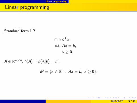
Standard form LP
min cT x
s.t. Ax = b,
x ≥ 0.
A ∈ Rm×n, h(A) = h(A|b) = m.
M = {x ∈ Rn : Ax = b, x ≥ 0}.
2017-02-27 3 / 40
Linear programming
Linear programming
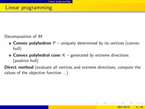
Decomposition of M:
Convex polyhedron P – uniquely determined by its vertices (convexhull)
Convex polyhedral cone K – generated by extreme directions(positive hull)
Direct method (evaluate all vertices and extreme directions, compute thevalues of the objective function ...)
2017-02-27 4 / 40
Linear programming
Linear programming trichotomy
One of these cases is valid:
1. M = ∅2. M 6= ∅: the problem is unbounded
3. M 6= ∅: the problem has an optimal solution (at least one of thesolutions is vertex)
2017-02-27 5 / 40
Primal simplex algorithm
Content
1 Linear programming
2 Primal simplex algorithm
3 Duality in linear programming
4 Dual simplex algorithm
5 Software tools for LP
2017-02-27 6 / 40

Primal simplex algorithm
1914–20052017-02-27 7 / 40
Primal simplex algorithm
Simplex algorithm – basis
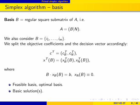
Basis B = regular square submatrix of A, i.e.
A = (B|N).
We also consider B = {i1, . . . , im}.We split the objective coefficients and the decision vector accordingly:
cT = (cTB , cTN ),
xT (B) = (xTB (B), xTN (B)),
whereB · xB(B) = b, xN(B) ≡ 0.
Feasible basis, optimal basis.
Basic solution(s).
2017-02-27 8 / 40
Primal simplex algorithm
Simplex algorithm – simplex table
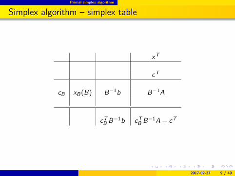
xT
cT
cB xB(B) B−1b B−1A
cTB B−1b cTB B−1A− cT
2017-02-27 9 / 40
Primal simplex algorithm
Simplex algorithm – simplex table
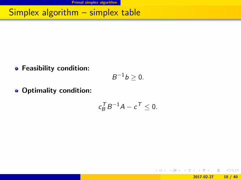
Feasibility condition:B−1b ≥ 0.
Optimality condition:
cTB B−1A− cT ≤ 0.
2017-02-27 10 / 40
Primal simplex algorithm
Simplex algorithm – a step
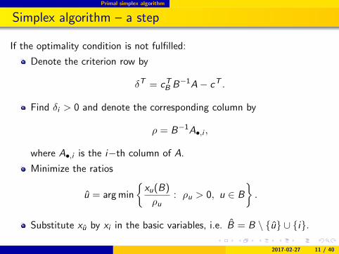
If the optimality condition is not fulfilled:
Denote the criterion row by
δT = cTB B−1A− cT .
Find δi > 0 and denote the corresponding column by
ρ = B−1A•,i ,
where A•,i is the i−th column of A.
Minimize the ratios
u = arg min
{xu(B)
ρu: ρu > 0, u ∈ B
}.
Substitute xu by xi in the basic variables, i.e. B = B \ {u} ∪ {i}.
2017-02-27 11 / 40
Primal simplex algorithm
Simplex algorithm – a step
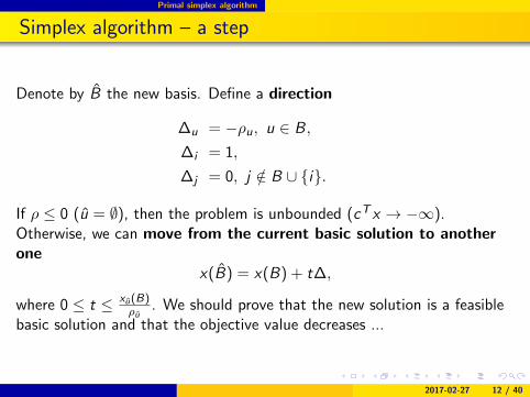
Denote by B the new basis. Define a direction
∆u = −ρu, u ∈ B,
∆i = 1,
∆j = 0, j /∈ B ∪ {i}.
If ρ ≤ 0 (u = ∅), then the problem is unbounded (cT x → −∞).Otherwise, we can move from the current basic solution to anotherone
x(B) = x(B) + t∆,
where 0 ≤ t ≤ xu(B)ρu
. We should prove that the new solution is a feasiblebasic solution and that the objective value decreases ...
2017-02-27 12 / 40
Primal simplex algorithm
Simplex algorithm – a step
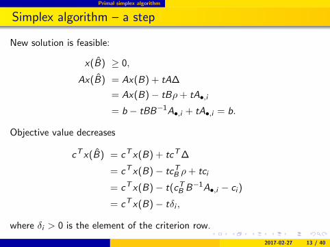
New solution is feasible:
x(B) ≥ 0,
Ax(B) = Ax(B) + tA∆
= Ax(B)− tBρ+ tA•,i
= b − tBB−1A•,i + tA•,i = b.
Objective value decreases
cT x(B) = cT x(B) + tcT∆
= cT x(B)− tcTB ρ+ tci
= cT x(B)− t(cTB B−1A•,i − ci )
= cT x(B)− tδi ,
where δi > 0 is the element of the criterion row.
2017-02-27 13 / 40
Primal simplex algorithm
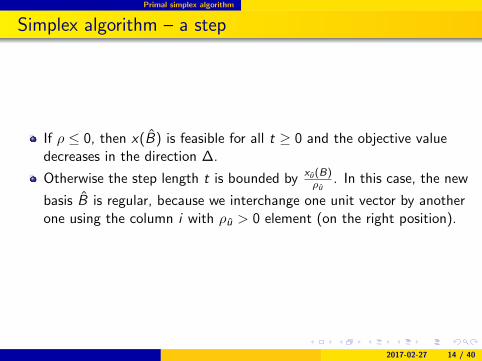
Simplex algorithm – a step
If ρ ≤ 0, then x(B) is feasible for all t ≥ 0 and the objective valuedecreases in the direction ∆.
Otherwise the step length t is bounded by xu(B)ρu
. In this case, the new
basis B is regular, because we interchange one unit vector by anotherone using the column i with ρu > 0 element (on the right position).
2017-02-27 14 / 40
Primal simplex algorithm
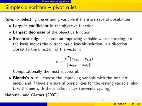
Simplex algorithm – pivot rules
Rules for selecting the entering variable if there are several possibilities:
Largest coefficient in the objective function
Largest decrease of the objective function
Steepest edge – choose an improving variable whose entering intothe basis moves the current basic feasible solution in a directionclosest to the direction of the vector c
maxcT (xnew − xold)
‖xnew − xold‖.
Computationally the most successful.
Blands’s rule – choose the improving variable with the smallestindex, and if there are several possibilities for the leaving variable, alsotake the one with the smallest index (prevents cycling)
Matousek and Gartner (2007).
2017-02-27 15 / 40
Primal simplex algorithm
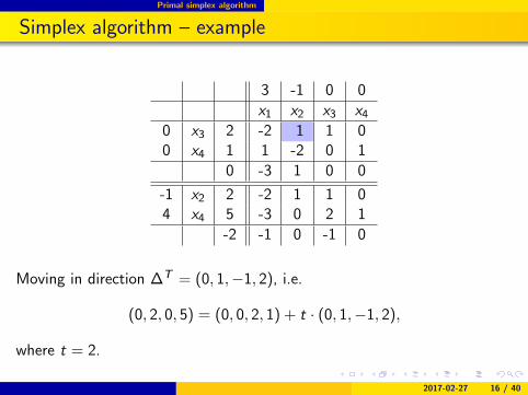
Simplex algorithm – example
3 -1 0 0
x1 x2 x3 x40 x3 2 -2 1 1 00 x4 1 1 -2 0 1
0 -3 1 0 0
-1 x2 2 -2 1 1 04 x4 5 -3 0 2 1
-2 -1 0 -1 0
Moving in direction ∆T = (0, 1,−1, 2), i.e.
(0, 2, 0, 5) = (0, 0, 2, 1) + t · (0, 1,−1, 2),
where t = 2.
2017-02-27 16 / 40
Primal simplex algorithm
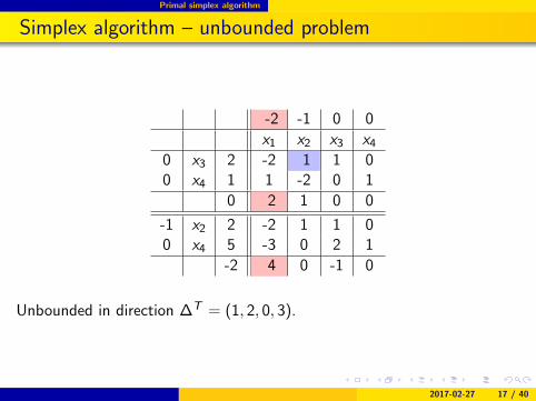
Simplex algorithm – unbounded problem
-2 -1 0 0
x1 x2 x3 x40 x3 2 -2 1 1 00 x4 1 1 -2 0 1
0 2 1 0 0
-1 x2 2 -2 1 1 00 x4 5 -3 0 2 1
-2 4 0 -1 0
Unbounded in direction ∆T = (1, 2, 0, 3).
2017-02-27 17 / 40
Duality in linear programming
Content
1 Linear programming
2 Primal simplex algorithm
3 Duality in linear programming
4 Dual simplex algorithm
5 Software tools for LP
2017-02-27 18 / 40
Duality in linear programming
Linear programming duality
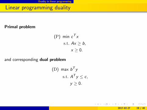
Primal problem
(P) min cT x
s.t. Ax ≥ b,
x ≥ 0.
and corresponding dual problem
(D) max bT y
s.t. AT y ≤ c ,
y ≥ 0.
2017-02-27 19 / 40
Duality in linear programming
Linear programming duality
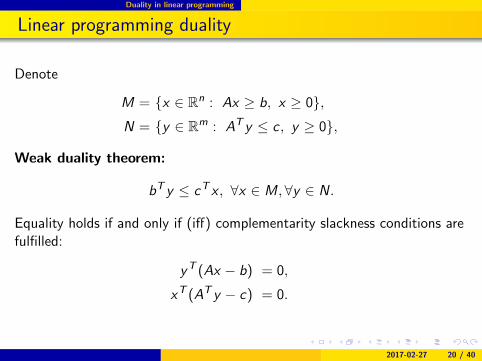
Denote
M = {x ∈ Rn : Ax ≥ b, x ≥ 0},N = {y ∈ Rm : AT y ≤ c, y ≥ 0},
Weak duality theorem:
bT y ≤ cT x , ∀x ∈ M,∀y ∈ N.
Equality holds if and only if (iff) complementarity slackness conditions arefulfilled:
yT (Ax − b) = 0,
xT (AT y − c) = 0.
2017-02-27 20 / 40
Duality in linear programming
Linear programming duality
Duality theorem: If M 6= ∅ and N 6= ∅, than the problems (P), (D)have optimal solutions.
Strong duality theorem: The problem (P) has an optimal solution ifand only if the dual problem (D) has an optimal solution. If oneproblem has an optimal solution, than the optimal values are equal.
2017-02-27 21 / 40
Duality in linear programming
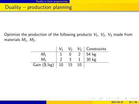
Duality – production planning
Optimize the production of the following products V1, V2, V3 made frommaterials M1, M2.
V1 V2 V3 Constraints
M1 1 0 2 54 kgM2 2 3 1 30 kg
Gain ($/kg) 10 15 10
2017-02-27 22 / 40
Duality in linear programming
Duality
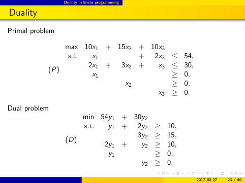
Primal problem
(P)
max 10x1 + 15x2 + 10x3s.t. x1 + 2x3 ≤ 54,
2x1 + 3x2 + x3 ≤ 30,x1 ≥ 0,
x2 ≥ 0,x3 ≥ 0.
Dual problem
(D)
min 54y1 + 30y2s.t. y1 + 2y2 ≥ 10,
3y2 ≥ 15,2y1 + y2 ≥ 10,y1 ≥ 0,
y2 ≥ 0.
2017-02-27 23 / 40
Duality in linear programming
Duality
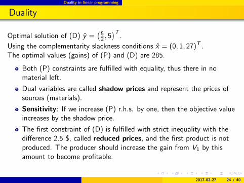
Optimal solution of (D) y =(52 , 5)T
.
Using the complementarity slackness conditions x = (0, 1, 27)T .The optimal values (gains) of (P) and (D) are 285.
Both (P) constraints are fulfilled with equality, thus there in nomaterial left.
Dual variables are called shadow prices and represent the prices ofsources (materials).
Sensitivity: If we increase (P) r.h.s. by one, then the objective valueincreases by the shadow price.
The first constraint of (D) is fulfilled with strict inequality with thedifference 2.5 $, called reduced prices, and the first product is notproduced. The producer should increase the gain from V1 by thisamount to become profitable.
2017-02-27 24 / 40
Duality in linear programming
Transportation problem
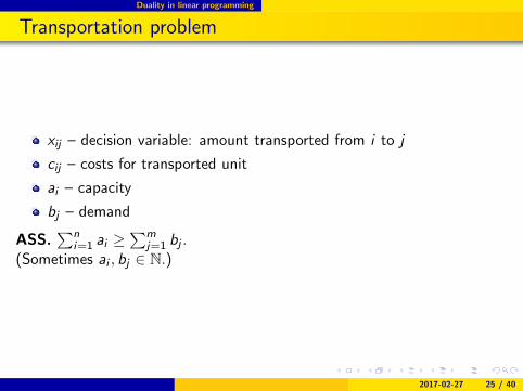
xij – decision variable: amount transported from i to j
cij – costs for transported unit
ai – capacity
bj – demand
ASS.∑n
i=1 ai ≥∑m
j=1 bj .(Sometimes ai , bj ∈ N.)
2017-02-27 25 / 40
Duality in linear programming
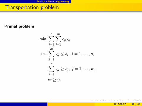
Transportation problem
Primal problem
minn∑
i=1
m∑j=1
cijxij
s.t.
m∑j=1
xij ≤ ai , i = 1, . . . , n,
n∑i=1
xij ≥ bj , j = 1, . . . ,m,
xij ≥ 0.
2017-02-27 26 / 40
Duality in linear programming
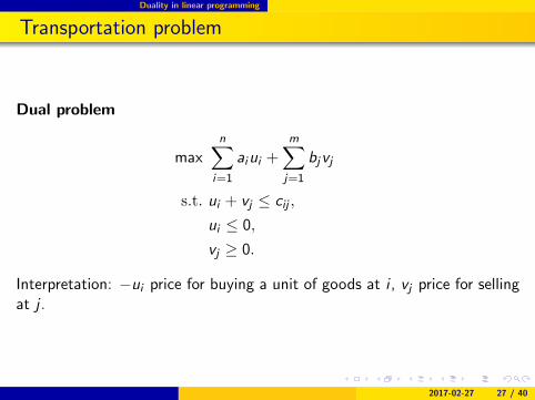
Transportation problem
Dual problem
maxn∑
i=1
aiui +m∑j=1
bjvj
s.t. ui + vj ≤ cij ,
ui ≤ 0,
vj ≥ 0.
Interpretation: −ui price for buying a unit of goods at i , vj price for sellingat j .
2017-02-27 27 / 40
Duality in linear programming
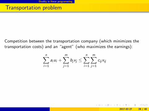
Transportation problem
Competition between the transportation company (which minimizes thetransportation costs) and an “agent” (who maximizes the earnings):
n∑i=1
aiui +m∑j=1
bjvj ≤n∑
i=1
m∑j=1
cijxij
2017-02-27 28 / 40

Duality in linear programming
Linear programming duality
Apply KKT optimality conditions to primal LP ... we will see relationswith NLP duality.
2017-02-27 29 / 40

Dual simplex algorithm
Content
1 Linear programming
2 Primal simplex algorithm
3 Duality in linear programming
4 Dual simplex algorithm
5 Software tools for LP
2017-02-27 30 / 40
Dual simplex algorithm
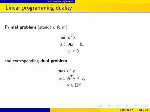
Linear programming duality
Primal problem (standard form)
min cT x
s.t. Ax = b,
x ≥ 0.
and corresponding dual problem
max bT y
s.t. AT y ≤ c ,
y ∈ Rm.
2017-02-27 31 / 40
Dual simplex algorithm
Dual simplex algorithm
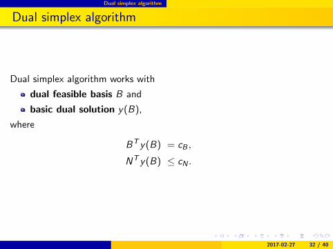
Dual simplex algorithm works with
dual feasible basis B and
basic dual solution y(B),
where
BT y(B) = cB ,
NT y(B) ≤ cN .
2017-02-27 32 / 40
Dual simplex algorithm
Dual simplex algorithm
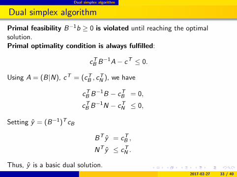
Primal feasibility B−1b ≥ 0 is violated until reaching the optimalsolution.Primal optimality condition is always fulfilled:
cTB B−1A− cT ≤ 0.
Using A = (B|N), cT = (cTB , cTN ), we have
cTB B−1B − cTB = 0,
cTB B−1N − cTN ≤ 0,
Setting y = (B−1)T cB
BT y = cTB ,
NT y ≤ cTN .
Thus, y is a basic dual solution.2017-02-27 33 / 40
Dual simplex algorithm
Dual simplex algorithm – a step
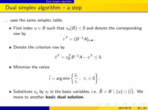
... uses the same simplex table.
Find index u ∈ B such that xu(B) < 0 and denote the correspondingrow by
τT = (B−1A)u,•.
Denote the criterion row by
δT = cTB B−1A− cT ≤ 0.
Minimize the ratios
i = arg min
{δiτi
: τi < 0
}.
Substitute xu by xi in the basic variables, i.e. B = B \ {u} ∪ {i}. Wemove to another basic dual solution.
2017-02-27 34 / 40
Dual simplex algorithm
Example – dual simplex algorithm
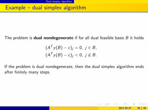
The problem is dual nondegenerate if for all dual feasible basis B it holds
(AT y(B)− c)j = 0, j ∈ B,
(AT y(B)− c)j < 0, j /∈ B.
If the problem is dual nondegenerate, then the dual simplex algorithm endsafter finitely many steps.
2017-02-27 35 / 40
Dual simplex algorithm
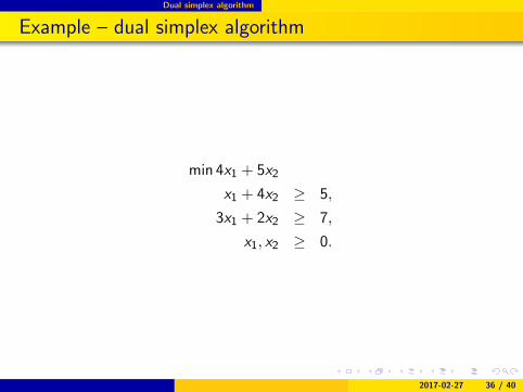
Example – dual simplex algorithm
min 4x1 + 5x2
x1 + 4x2 ≥ 5,
3x1 + 2x2 ≥ 7,
x1, x2 ≥ 0.
2017-02-27 36 / 40
Dual simplex algorithm
Example – dual simplex algorithm
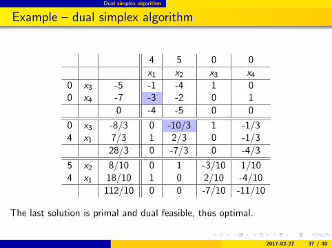
4 5 0 0
x1 x2 x3 x40 x3 -5 -1 -4 1 00 x4 -7 -3 -2 0 1
0 -4 -5 0 0
0 x3 -8/3 0 -10/3 1 -1/34 x1 7/3 1 2/3 0 -1/3
28/3 0 -7/3 0 -4/3
5 x2 8/10 0 1 -3/10 1/104 x1 18/10 1 0 2/10 -4/10
112/10 0 0 -7/10 -11/10
The last solution is primal and dual feasible, thus optimal.
2017-02-27 37 / 40

Software tools for LP
Content
1 Linear programming
2 Primal simplex algorithm
3 Duality in linear programming
4 Dual simplex algorithm
5 Software tools for LP
2017-02-27 38 / 40

Software tools for LP
Software tools for LP
Matlab
Mathematica
GAMS
Cplex studio
AIMMS
...
R
MS Excel
...
2017-02-27 39 / 40
Software tools for LP
Literature
Bazaraa, M.S., Sherali, H.D., and Shetty, C.M. (2006). Nonlinear programming:theory and algorithms, Wiley, Singapore, 3rd edition.
Boyd, S., Vandenberghe, L. (2004). Convex Optimization, Cambridge UniversityPress, Cambridge.
P. Lachout (2011). Matematicke programovanı. Skripta k (zanikle) prednasceOptimalizace I (IN CZECH).
Matousek and Gartner (2007). Understanding and using linear programming,Springer.
2017-02-27 40 / 40


![aumwno I - DTICWith Wolfe's simplex method of quadratic programming [18] and Dorn's analysis of duality in quadratic programing [8], the stage was set for 4 the extension of decomposition](https://img.pdfslide.us/doc/110x75/5e95907915db0a427c021c79/aumwno-i-dtic-with-wolfes-simplex-method-of-quadratic-programming-18-and-dorns.jpg)