Embed Size (px)
Citation preview
Copyright c© 2006 Tech Science Press CMES, vol.13, no.1, pp.19-34, 2006
Linear Buckling Analysis of Shear Deformable Shallow Shells by the BoundaryDomain Element Method
P.M. Baiz1 and M.H. Aliabadi1
Abstract: In this paper the linear buckling problem ofelastic shallow shells by a shear deformable shell theoryis presented. The boundary domain integral equationsare obtained by coupling two dimensional plane stresselasticity with boundary element formulation of Reissnerplate bending. The buckling problem is formulated as astandard eigenvalue problem, in order to obtain directlycritical loads and buckling modes as part of the solu-tion. The boundary is discretised into quadratic isopara-metric elements while in the domain quadratic quadrilat-eral cells are used. Several examples of cylindrical shal-low shells (curved plates) with different dimensions andboundary conditions are analysed. The results are com-pared with finite element solutions, and very good agree-ment is obtained.
keyword: Shallow Shell, Buckling, Shear DeformableTheory, Boundary Element Method.
1 Introduction
The behavior of curved plates under compression loads isof major concern in areas such as aerospace, in which thedesign requirements of weight critical applications usu-ally leads to thin panels with stability problems.
The first study of stability of shells can be traced backin 1911 by Lorenz, in which he presented solutions forcylinders subjected to axial compression. More com-plete descriptions of shell stability have been presentedby Timoshenko and Gere (1961) for several classicalproblems, and by Brush and Almorth (1975) for nonlin-ear theories. Other works dealing with shell buckling canbe found in Gerard and Becker (1957), giving an overallview of shell buckling problems; Nash’s review [Nash(1966)] with several hundred papers on shell buckling;Singer (1982) who reports on experimental investigationsand Bushnell (1985) who concentrates on numerical pro-cedures for the modeling and solution of complex non-
1 Imperial College London, South Kensington, SW7 2BT, London,U.K.
linear problems. Other more recent and useful bibliogra-phies and review papers can be found in works by Noor(1990), Teng (1996) and Knight and Starnes (1997).
The applications of the Boundary Element Method(BEM) to stability problems for plate and shallow shellstructures have been investigated since the 80’s. Manolis,Beskos, and Pineros (1986) developed a direct bound-ary element formulation dealing with linear elastic sta-bility analysis of Kirchhoff plates. More recently, Syn-gellakis and Elzein (1994) presented an extended bound-ary element formulation to incorporate any combina-tion of loading and support conditions; Nerantzaki andKatsikadelis (1996) presented a boundary element for-mulation for buckling of plates with variable thickness;and Lin, Duffield, and Shih (1999) described a gen-eral boundary element formulation for different bound-ary conditions and arbitrary planar shapes.
In the case of post-buckling formulations for thin elasticplates O’Donoghue and Atluri (1987) introduced the firstboundary element approach to nonlinear plate analysis;while for thin shallow shells, Zhang and Atluri (1988)presented a boundary element formulation applied to theanalysis of snap-through phenomena. In all these cases,plate and shallow shell BEM formulations have used theClassical or Kirchhoff-Love theory.
Although for most practical applications the classicaltheory is sufficient; it has been shown by Reissner (1947)that Kirchhoff theory of thin plates is not in agreementwith the experimental results for problems with stressconcentrations (stresses at an edge of a hole when thehole diameter became so small as to be of the order ofmagnitude of the plate thickness); or also in the caseof composite shells, where the ratio of Young’s modu-lus to shear modulus can be very large (low transverseshear modulus compared to isotropic materials). There-fore, shell theories accounting transverse shear deforma-tion overcome problems associated with the applicationof the classical theory, and additionally can be used forthe analysis of thin and thick shells.
20 Copyright c© 2006 Tech Science Press CMES, vol.13, no.1, pp.19-34, 2006
Recent developments with shear deformable plate the-ory by BEM include de works of Purbolaksono and Ali-abadi (2005b) for large deformation; Wen, Aliabadi, andYoung (2006) for post-buckling; and Supriyono and Ali-abadi (2006) for combined large deflection and plasticity.
Application of shear deformable theory to the linear elas-tic buckling problem of plates using the boundary el-ement method has been presented recently by Purbo-laksono and Aliabadi (2005a); and to the best knowl-edge of the authors, no study on the linear elastic buck-ling analysis of shallow shell structures by BEM hasbeen reported, for classical (Kirchhoff-Love) or shear de-formable (Reissner or Mindlin) theories. Other works onplates and shells by BEM can be found in Beskos (1991),and recent advances in BEM and their solid mechanicsapplications are in Aliabadi (2002).
The present paper reports on the investigation of a newboundary domain element formulation for the bucklinganalysis of shear deformable shallow shells. Initially,basic concepts of shear deformable shallow shells, andboundary integral equations are described. The bucklingproblem is formulated as a standard eigenvalue problem,to provide direct evaluation of critical load factors andbuckling modes. Numerical procedure to solve the for-mulation is presented, first the in plane stresses at domainpoints are calculated and subsequently the boundary inte-gral equations for the buckling problem are solved. Sev-eral examples in which results from the proposed BEMformulation are compared with FEM results and goodagreements are obtained.
2 Boundary domain integral equations for shear de-formable shallow shells
Consider a shallow shell of an isotropic linear elasticmaterial, with uniform thickness h, Young’s modulus E,Poisson ratio v and shear modulus G = E/2(1+v), with aquadratic middle surface defined by R1 and R2, which areprincipal curvatures of the shell in the x1− and x2− direc-tions, respectively. The indicial notation used throughoutthis paper is as follows: the Greek indices (α,β,γ) willvary from 1 to 2 and Roman indices (i, j,k) from 1 to 3.
Equilibrium equations for shear deformable plate bend-ing (Reissner-Mindlin) and 2D elasticity for shallowshells can be written in indicial notation as follows Ali-abadi (2002):
Mαβ,β −Qα = 0; (1)
Qα,α −kαβNαβ +q3 = 0; (2)
Nαβ,β +qα = 0 (3)
where k11 = 1/R1, k22 = 1/R2 and k12 = k21 = 0; (),β= ∂( )/∂xβ. Nαβ denote membrane stresses, Mαβ rep-resent bending moments, Qα is the shear forces for platebending and qi are the body forces.
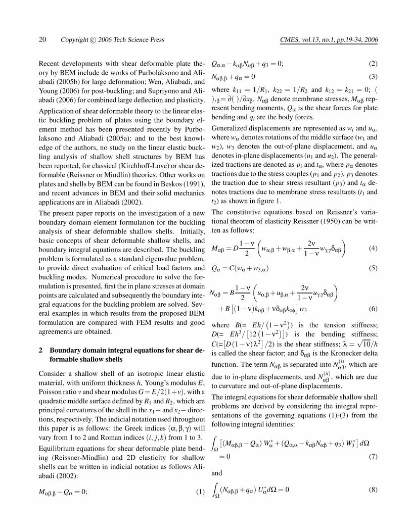
Generalized displacements are represented as wi and uα,where wα denotes rotations of the middle surface (w1 andw2), w3 denotes the out-of-plane displacement, and uαdenotes in-plane displacements (u1 and u2). The general-ized tractions are denoted as pi and tα, where pα denotestractions due to the stress couples (p1 and p2), p3 denotesthe traction due to shear stress resultant (p3) and tα de-notes tractions due to membrane stress resultants (t1 andt2) as shown in figure 1.
The constitutive equations based on Reissner’s varia-tional theorem of elasticity Reissner (1950) can be writ-ten as follows:
Mαβ = D1−ν
2
(wα,β +wβ,α +
2ν1−ν
wγ,γδαβ
)(4)
Qα = C(wα +w3,α) (5)
Nαβ = B1−ν
2
(uα,β +uβ,α +
2ν1−ν
uγ,γδαβ
)+B
[(1−ν)kαβ +νδαβkφφ
]w3 (6)
where B(= Eh/(1−ν2
)) is the tension stiffness;
D(= Eh3/[12
(1−ν2
)]) is the bending stiffness;
C(=[D(1−ν)λ2
]/2) is the shear stiffness; λ =
√10/h
is called the shear factor; and δαβ is the Kronecker delta
function. The term Nαβ is separated into N(i)αβ, which are
due to in-plane displacements, and N(ii)αβ , which are due
to curvature and out-of-plane displacements.
The integral equations for shear deformable shallow shellproblems are derived by considering the integral repre-sentations of the governing equations (1)-(3) from thefollowing integral identities:Z
Ω
[(Mαβ,β −Qα) W ∗
α +(Qα,α −kαβNαβ +q3) W ∗3
]dΩ
= 0 (7)
andZ
Ω(Nαβ,β +qα) U∗
αdΩ = 0 (8)
Linear Buckling Analysis 21
Figure 1 : Sign convection for generalised displacement and tractions.
where U∗α and W ∗
i (i = α,3) are weighting functions andΩ is the projected domain of a shell on x1 − x2 plane,bounded by boundary Γ. Equation (7) is an integral rep-resentation related to the governing equations for bend-ing and transverse shear stress resultants, while equation(8) is an integral representation related to the governingequations for membrane stress resultants.
2.1 Rotations and out of plane integral equations
The boundary domain integral representation related tothe governing equations for bending and transverse shearstress resultants of a boundary source point x′ are de-rived by using the weighted residual method as shown inDirgantara and Aliabadi (1999) and Dirgantara (2002).After taking into account all the limits and the jumpterms:
ci j(x′)wj(x′)+Z
Γ−P∗
i j(x′,x)wj (x)dΓ(x)
=Z
ΓW ∗
i j(x′,x)p j (x)dΓ(x)
−Z
ΓW ∗
i3
(x′,x
)kαβB
1−ν2
×[uα (x)nβ +uβ (x)nα +
2ν1−ν
uγ (x)nγδαβ
]dΓ(x)
+Z
ΩkαβB
1−ν2
[uα (X)W ∗
i3,β(x′,X
)+uβ (X)W ∗
i3,α(x′,X
)+
2ν1−ν
uγ (X)W ∗i3,γ
(x′,X
)δαβ
]dΩ(X)
−Z
ΩW ∗
i3
(x′,X
)kαβB×
[(1−ν)kαβ +νδαβkγγ
]w3 (X)dΩ(X)
+Z
ΩW ∗
i3(x′,X)q3(X)dΩ(X) (9)
whereR− denotes a Cauchy principal value integral,
x′,x ∈ Γ, X ∈ Ω are source and field points respectively,ci j(x′) are the jump terms, nβ are the components of theoutward normal vector to the shell boundary. The valueof ci j(x′) is equal to 1
2 δi j when x′ is located on a smoothboundary and equal to δi j when collocation is at domainpoints X.
W ∗i j and P∗
i j are the displacement and traction fundamentalsolutions respectively, derived by Vander Weeen (1982)and W ∗
i3,β is the derivative of the displacement fundamen-tal solutions with respect to the field point X. All thesekernels are given in appendix A.
2.2 In plane displacement integral equations
In the same way, the boundary domain integral equationrelated to the governing equations for membrane stressresultants of a boundary source point x′ can be written asDirgantara and Aliabadi (1999), Dirgantara (2002):
cθα(x′
)uα(x′)+
ZΓ− T ∗(i)
θα (x′,x)uα(x)dΓ(x)
+Z
ΩU∗
θα,β(x′,X)B[kαβ (1−ν)+νδαβkγγ
]w3(X)dΩ(X)
=Z
ΓU∗
θα(x′,x)tα(x)dΓ(x)+Z
ΩU∗
θα(x′,X)qα(X)dΩ(X)
(10)
where U∗θα and T (i)∗
θα are the well known fundamental so-lutions for in-plane displacements and membrane trac-
22 Copyright c© 2006 Tech Science Press CMES, vol.13, no.1, pp.19-34, 2006
tions respectively, while U∗θα,β is the derivative of the dis-
placement fundamental solution with respect to the fieldpoint X. These kernels are also given in appendix A. Theupper index (i) on T ∗
θα refers to the in plane displacement,
as it was explained with N(i)αβ.
Equations (9) and (10) represent the five boundary-domain integral equations for shear deformable shallowshell theory, the first two are in (9) (i = 1,2) and are forrotations (w1 and w2), the third (i = 3) also in (9) is forthe out-of-plane displacement (w3). The last two are in(10) (θ = 1,2) and are for in-plane displacements (u1 andu2).
It is important to mention that due to the curvature terms(containing kαβ), equations (9) and (10) have to be solvedsimultaneously and not only for collocation on boundarypoints x but also on domain points X.
3 Governing integral equations for linear bucklingof shear deformable shallow shells
In this section the buckling phenomenon of shallowshells is studied, initially the membrane stress resultantsin the domain are considered to be unknown due to ex-ternal loads on the boundary; therefore, determination ofmembrane stress resultants in the domain is the first stepsolution for the analysis. Next, the shell buckling equa-tions are obtained by introducing multiplication factorsof body forces or transverse loads (λ) in the governingintegral equations.
3.1 Integral equations for in plane stresses
The membrane stress resultants at domain points X′ canbe evaluated from the derivative of equation (10) and byusing the relationship in equation (6), resulting in the fol-lowing boundary-domain integral equation:
Nαβ(X′) =
ZΓ
U∗αβγ(X′,x)tγ(x)dΓ(x)
−Z
ΓT ∗
αβγ(X′,x)uγ(x)dΓ(x)
−Z
Ω− U∗
αβγ,θ(X′,X)B[kγθ (1−ν)+νδγθkφφ
]×w3(X)dΩ(X)+ fαβ(w3
(X′))
+Z
ΩU∗
αβγ(X′,X)qγ(X)dΩ(X)
+B[(1−ν)kαβ +νδαβkφφ
]w3
(X′) (11)
The kernels U∗αβγ and T ∗
αβγ in equation (11) are linear
combination of the first derivatives of U∗αβ and T ∗
αβ withrespect to the source point X′ and can be found in Dirgan-tara and Aliabadi (1999), Dirgantara (2002) and are alsolisted in appendix A. U∗
αβγ,θ is the derivative of U∗αβγ with
respect to the field point X and is given in appendix A.
The term fαβ in equation (11) arises from the integrationof the curvature term over the surface Γ′ centered at theload point X′. Details of the procedure to obtain this termare given in appendix B.
Another approach that could be used for the evaluation ofstresses at internal points consist of a numerical differen-tiation of displacements by means of the shape functionsof the domain cells, after internal displacement have beenfound, Zhang and Atluri (1988). The boundary-domainintegral equation (11) although computational more timeconsuming and mathematically more cumbersome, givesmore accurate results and therefore it was adopted in thiswork.
3.2 Integral formulation for the linear buckling prob-lem
Appropriate forms of the linearized buckling problemcan be derived by transforming the shell integral equa-tion (9) into an equivalent shell buckling formulation andintroducing a critical load factor λ, resulting in a group ofequation in terms of the prebuckling membrane stressesand the buckled shell displacements, as follows:
ci j(x′)wj(x′)+Z
Γ−P∗
i j(x′,x)wj (x)dΓ(x)
=Z
ΓW ∗
i j(x′,x)p j (x)dΓ(x)
−Z
ΓW ∗
i3
(x′,x
)kαβB
1−ν2
×[uα (x)nβ +uβ (x)nα +
2ν1−ν
uγ (x)nγδαβ
]dΓ(x)
+Z
ΩkαβB
1−ν2
[uα (X)W ∗
i3,β(x′,X
)+uβ (X)W ∗
i3,α(x′,X
)+
2ν1−ν
uγ (X)W ∗i3,γ
(x′,X
)δαβ
]dΩ(X)
−Z
ΩW ∗
i3
(x′,X
)kαβB
((1−ν)kαβ +νδαβkφφ
)×w3 (X)dΩ(X)
Linear Buckling Analysis 23
+λZ
ΩW ∗
i3(x′,X)q3(X)dΩ(X)
+λZ
ΩW ∗
i3(x′,X)(Nαβw3,β),α(X)dΩ(X) (12)
where (Nαβw3,β),α is a body term due to the large deflec-tion of w3(X). This term is the common extra term thatappears in the nonlinear equilibrium equations of platesand shells (e.g. see the nonlinear equilibrium equation6.10 in Brush and Almorth (1975)).
It is important to notice again that because of the pres-ence of the curvature terms in (12), this equation has tobe solve simultaneously with equation (10).
The deflection equation w3 at the domain points X′ is re-quired as the additional equation to arrange an eigenvalueequation, as follows:
w3(X′) =Z
ΓW ∗
3 j(X′,x)p j (x)dΓ(x)
−Z
ΓP∗
3 j(X′,x)wj (x)dΓ(x)
−Z
ΓW ∗
33
(X′,x
)kαβB
1−ν2
×[uα (x)nβ +uβ (x)nα +
2ν1−ν
uγ (x)nγδαβ
]dΓ(x)
+Z
ΩkαβB
1−ν2
[uα (X)W ∗
33,β(X′,X
)+uβ (X)W ∗
33,α(X′,X
)+
2ν1−ν
uγ (X)W ∗33,γ
(X′,X
)δαβ
]dΩ(X)
−Z
ΩW ∗
33
(X′,X
)kαβB
((1−ν)kαβ +νδαβkφφ
)×w3 (X)dΩ(X)
+λZ
ΩW ∗
33(X′,X)q3(X)dΩ(X)
+λZ
ΩW ∗
33(X′,X)(Nαβw3,β),α(X)dΩ(X) (13)
To arrange an eigenvalue equation, the derivativesw3,β(X) and w3,αβ(X) have to be expressed in terms ofw3(X), see section 4.3. Therefore the last integrals inequations (12) and (13), can be expressed as follows:
ci j(x′)wj(x′)+Z
Γ−P∗
i j(x′,x)wj (x)dΓ(x)
=Z
ΓW ∗
i j(x′,x)p j (x)dΓ(x)
−Z
ΓW ∗
i3
(x′,x
)kαβB
1−ν2
×
[uα (x)nβ +uβ (x)nα +
2ν1−ν
uγ (x)nγδαβ
]dΓ(x)
+Z
ΩkαβB
1−ν2
[uα (X)W ∗
i3,β(x′,X
)+uβ (X)W ∗
i3,α(x′,X
)+
2ν1−ν
uγ (X)W ∗i3,γ
(x′,X
)δαβ
]dΩ(X)
−Z
ΩW ∗
i3
(x′,X
)kαβB
((1−ν)kαβ +νδαβkφφ
)×w3 (X)dΩ(X)
+λZ
ΩW ∗
i3(x′,X) fb(X)dΩ(X) (14)
and,
w3(X′) =Z
ΓW ∗
3 j(X′,x)p j (x)dΓ(x)
−Z
ΓP∗
3 j(X′,x)wj (x)dΓ(x)
−Z
ΓW ∗
33
(X′,x
)kαβB
1−ν2
×[uα (x)nβ +uβ (x)nα +
2ν1−ν
uγ (x)nγδαβ
]dΓ(x)
+Z
ΩkαβB
1−ν2
[uα (X)W ∗
33,β(X′,X
)+uβ (X)W ∗
33,α(X′,X
)+
2ν1−ν
uγ (X)W ∗33,γ
(X′,X
)δαβ
]dΩ(X)
−Z
ΩW ∗
33
(X′,X
)kαβB
((1−ν)kαβ +νδαβkφφ
)×w3 (X)dΩ(X)
+λZ
ΩW ∗
33(X′,X) fb(X)dΩ(X) (15)
where:
fb = q3 +Nαβ,αf(r),βF−1w3 +Nαβf(r),αf(r),βF−1w3 (16)
4 Numerical implementation
In order to solve the integral equations presented in theprevious section, the boundary Γ and the domain Ω mustbe discretized. Generally, BEM formulations rely oncontinuous boundary elements and cells. However, be-cause of the presence of singular integrals in the domainduring the evaluation of the stresses Nαβ, it was decidedto implement continuous and discontinuous (partially ortotally) quadrilateral internal cells; while on the bound-ary semi-discontinuous elements are used for corners to
24 Copyright c© 2006 Tech Science Press CMES, vol.13, no.1, pp.19-34, 2006
avoid difficulties with discontinuity of the tractions atcorners.
From the implementation point of view, the use of dis-continuous or semi discontinuous elements requires theconsideration of two different meshes: the geometricmesh, defined by the geometric nodes which always lieon the boundary of the element; and the functional mesh,defined by the functional nodes which can exist any-where within the element boundaries. In the domain thisdistinction allows the use of a whole range of quadrilat-eral cell elements by just defining an appropriate set ofparameters, as it will be explained later.
4.1 Discretization
In the present study, quadratic isoparametric boundaryelements are used to describe the geometry and the func-tion along Γ. In the same way for the domain, quadraticquadrilateral isoparametric elements are used to describethe geometry and the function over Ω.
Equation (9) can be rewritten in a discretized form as:
ci j(x′)wj(x′)+Ne
∑n=1
3
∑m=1
wnmj
Z ξ=+1
ξ=−1P∗
i j(x′,x)Φm(ξ)Jn(ξ)dξ
=Ne
∑n=1
3
∑m=1
pnmj
Z ξ=+1
ξ=−1W ∗
i j(x′,x)Φm(ξ)Jn(ξ)dξ
−Ne
∑n=1
3
∑m=1
kαβB1−ν
2
(unm
α nnmβ +unm
β nnmα
+2ν
1−νunm
γ nnmγ δαβ
)×
Z ξ=+1
ξ=−1W ∗
i3
(x′,x
)Φm(ξ)Jn(ξ)dξ
+Nc
∑k=1
9
∑l=1
kαβB1−ν
2ukl
α
Z η=+1
η=−1
Z ξ=+1
ξ=−1W ∗
i3,β(x′,X
)×Ψl(ξ,η)Jk(ξ,η)dξdη
+Nc
∑k=1
9
∑l=1
kαβB1−ν
2ukl
β
Z η=+1
η=−1
Z ξ=+1
ξ=−1W ∗
i3,α(x′,X
)×Ψl(ξ,η)Jk(ξ,η)dξdη
+Nc
∑k=1
9
∑l=1
kααBνuklγ
Z η=+1
η=−1
Z ξ=+1
ξ=−1W ∗
i3,γ(x′,X
)×Ψl(ξ,η)Jk(ξ,η)dξdη
−Nc
∑k=1
9
∑l=1
kαβB[(1−ν)kαβ +νδαβkγγ
]wkl
3 ×Z η=+1
η=−1
Z ξ=+1
ξ=−1W ∗
i3
(x′,X
)Ψl(ξ,η)Jk(ξ,η)dξdη
+Nc
∑k=1
9
∑l=1
qkl3
Z η=+1
η=−1
Z ξ=+1
ξ=−1W ∗
i3
(x′,X
)×Ψl(ξ,η)Jk(ξ,η)dξdη (17)
where Ne and Nc are number of boundary elements andinternal cells respectively. Φm are the boundary shapefunctions. Ψl are the domain shape functions. ξ andη are local coordinates. Jn and Jk are the Jacobian oftransformation for boundary elements and internal cellsrespectively. A complete description of the boundary el-ements and domain cells used in this work is given inAppendix C.
Equations (10,14 and 15) have also to be expressed in thesame way as equation (17), but for the sake of space thecomplete expression will not be shown here.
In the case of the domain integral that contains fb inequations (14 and 15), when q3 = 0, the integral can bediscretized as follows:ZΩ
W ∗i3(x′,X) fb(X)dΩ(X)
=Nc
∑k=1
9
∑l=1
wkl3 · f kl
bw
Z η=+1
η=−1
Z ξ=+1
ξ=−1W ∗
i3
(x′,X
)×Ψl(ξ,η)Jk(ξ,η)dξdη (18)
where f klbw = Nkl
αβ,αf(r),βF−1 +Nklαβf(r),αf(r),βF−1.
4.2 Treatment of the integrals
Generally speaking, two different kinds of integrals canbe defined for both the boundary and domain. Dependingon the integrands, integrals can be classified as: Regular,in which case they can be evaluated using the standardgauss quadrature rule or; Singular, when the collocationpoint belongs to the element over which the integration isperformed, in this case special techniques must be used.
All the singular integrals appearing in the displacementand internal stress integral equations are dealt with by us-ing well established techniques and are treated separatelybased on their order of singularity.
On the boundary, near singular integrals (when the col-location node is close to the integration element) aretreated with the element subdivision technique Aliabadi(2002). Weakly singular integrals O(lnr) are treated us-ing a nonlinear coordinate transformation as reported byTelles Telles (1987). Strong singular integrals O(1/r) arecomputed indirectly by considering the generalized rigidbody motion, as explained in Dirgantara (2002).
Linear Buckling Analysis 25
The domain singular integrals can also be separated inweakly O(1/r) and strong O(1/r2). Weak singular in-tegrals are treated by a simple technique such as polarcoordinate transformation, followed by a regular proce-dure Aliabadi (2002). Strong singular integrals requirespecial techniques such as the ones described by LeitaoLeitao (1994).
4.3 Evaluation of the derivative terms
Several derivative terms in the domain have to be ob-tained, and although this procedure could be performedwith the polynomial interpolation of the domain cells, itwas considered more convenient the use of radial basisfunctions f (r) in order to establish the same frame ofcomparison with an only boundary formulation that willbe developed in a future publication.
The derivative terms w3,β(X) and w3,αβ(X) are approxi-mated as follows:
w3(x1,x2) =L
∑m=1
f (r)mΨm (19)
where the radial basis function is chosen as f (r) =√c2 + r2 and c2 =2. L is the total number of selected
points in the domain, which are the same domain pointsused in the domain integration process. As it can be seenfrom the integral equations (14) and (15), some of the in-tegrals are on the domain Ω, for which quadratic isopara-metric quadrilateral domain cells of 9 nodes are used.
The distance r in equation (19) is given by the followingexpression:
r =√
(x1 −xm1 )2 +(x2 −xm
2 )2 (20)
The Ψm are coefficients determined by values at the Ldomain points:
ΨΨΨ = F−1w3 (21)
Consequently, the first derivative of deflection w3,β canbe expressed as the product of the first derivative of theradial basis function and the coefficients Ψm, as follows:
w3,β(x1,x2) = f(r),βF−1w3 (22)
In the same way, the second derivative of deflection w3,αβcan be written as:
w3,αβ(x1,x2) = f(r),βf(r),αF−1w3 (23)
Similar to the above expressions, the derivative of in-plane stress resultants Nαβ,α can be expressed as:
Nαβ,α(x1,x2) = f(r),αF−1Nαβ (24)
5 Numerical procedure
In this section a numerical procedure developed to solvethe equations shown in the previous sections is explained.The solution steps towards the linear buckling solutionare given as follows:
• Initially, solution of the linear shallow shell bound-ary integral equations (9) and (10) is obtained.
• After boundary and domain displacements as wellas boundary tractions are known, the membranestresses at domain nodes Nαβ(X′) are obtained fromequation (11).
• Approximated derivatives of membrane stresses andout of plane displacement are obtained, as explainedin the subsection 4.3.
• Finally, the boundary integral equations of the buck-ling problem (10), (14) and (15) are assembled andsolved; obtaining buckling modes and buckling loadfactors.
This procedure is explained with more detail in the fol-lowing subsections.
5.1 Shell in plane stresses
After discretized equations (9) and (10) as explained insection 4.1, and point collocation the following linearsystem of equations is obtained for every node:⎡⎢⎢⎢⎢⎣
· · ·· · ·· · ·· · ·· · ·
c+Hp Hp Hpw Hu Hu
Hp c+Hp Hpw Hu Hu
Hp Hp c+Hpw Hu Hu
0 0 Hw c+Hs Hs
0 0 Hw Hs c+Hs
· · ·· · ·· · ·· · ·· · ·
⎤⎥⎥⎥⎥⎦
5×5(N+L)
⎧⎪⎪⎪⎪⎪⎪⎪⎪⎪⎪⎨⎪⎪⎪⎪⎪⎪⎪⎪⎪⎪⎩
...w1
w2
w3
u1
u2...
⎫⎪⎪⎪⎪⎪⎪⎪⎪⎪⎪⎬⎪⎪⎪⎪⎪⎪⎪⎪⎪⎪⎭
5(N+L)
26 Copyright c© 2006 Tech Science Press CMES, vol.13, no.1, pp.19-34, 2006
=
⎡⎢⎢⎢⎢⎣
· · ·· · ·· · ·· · ·· · ·
Gp Gp Gp 0 0Gp Gp Gp 0 0Gp Gp Gp 0 00 0 0 Gs Gs
0 0 0 Gs Gs
· · ·· · ·· · ·· · ·· · ·
⎤⎥⎥⎥⎥⎦
5×15NE
×
⎧⎪⎪⎪⎪⎪⎪⎪⎪⎪⎪⎨⎪⎪⎪⎪⎪⎪⎪⎪⎪⎪⎩
...p1
p2
p3
t1t2...
⎫⎪⎪⎪⎪⎪⎪⎪⎪⎪⎪⎬⎪⎪⎪⎪⎪⎪⎪⎪⎪⎪⎭
15NE
+
⎧⎪⎪⎪⎪⎨⎪⎪⎪⎪⎩
b1
b2
b3
g1
g2
⎫⎪⎪⎪⎪⎬⎪⎪⎪⎪⎭
(25)
where bi are the product of the bending displacement fun-damental solutions with the domain load q3, which inthis study is set to zero (q3 = 0 → bi = 0). Similarlygα are the product of the membrane displacement fun-damental solutions with the in plane domain loads qα,which are also set to zero in this analysis (qα = 0). Hand G are boundary element matrices for tractions anddisplacements fundamental solutions, respectively. Theindexes p and s on H and G refer to plate bending andplane stress formulations respectively; while the indexesu and w are coupled terms between plate bending andplane stress formulations. N, L and NE are number ofboundary nodes, domain points and boundary elements,respectively.
After performing all the collocation process, the knownand unknown quantities in equation (25) can be arrangedas a set of linear algebraic equation:
[A]5(N+L)×5(N+L) {X}5(N+L) = {F}5(N+L) (26)
where [A] is the system matrix, {X} contains the un-knowns displacements and tractions on the boundary N,as well as all the displacement in the domain L. The vec-tor {F} is obtained by multiplying the related matrices ofH or G by the known values of wi, uα or pi, tα (becausethe body forces where set to zero, qi = 0).
Once equation (26) has been solved, in-plane stressesN11, N12, and N22 in the domain are calculated from equa-tion (11). They are required to solve the shell bucklingproblem.
5.2 Shell buckling problem
After discretization of the equations (10) and (14) asexplained in section 4.1, the linear system of algebraic
equations for every collocation node on the boundary canbe written similar to the linear shell solution:⎡⎢⎢⎢⎢⎣
· · ·· · ·· · ·· · ·· · ·
c+Hp Hp Hpw Hu Hu
Hp c+Hp Hpw Hu Hu
Hp Hp c+Hpw Hu Hu
0 0 Hw c+Hs Hs
0 0 Hw Hs c+Hs
· · ·· · ·· · ·· · ·· · ·
⎤⎥⎥⎥⎥⎦
5×(5N+3L)
⎧⎪⎪⎪⎪⎪⎪⎪⎪⎪⎪⎨⎪⎪⎪⎪⎪⎪⎪⎪⎪⎪⎩
...w1
w2
w3
u1
u2...
⎫⎪⎪⎪⎪⎪⎪⎪⎪⎪⎪⎬⎪⎪⎪⎪⎪⎪⎪⎪⎪⎪⎭
5N+3L
=
⎡⎢⎢⎢⎢⎣
· · ·· · ·· · ·· · ·· · ·
Gp Gp Gp 0 0Gp Gp Gp 0 0Gp Gp Gp 0 00 0 0 Gs Gs
0 0 0 Gs Gs
· · ·· · ·· · ·· · ·· · ·
⎤⎥⎥⎥⎥⎦
5×15NE⎧⎪⎪⎪⎪⎪⎪⎪⎪⎪⎪⎨⎪⎪⎪⎪⎪⎪⎪⎪⎪⎪⎩
...p1
p2
p3
t1t2...
⎫⎪⎪⎪⎪⎪⎪⎪⎪⎪⎪⎬⎪⎪⎪⎪⎪⎪⎪⎪⎪⎪⎭
15NE
+λ
⎡⎢⎢⎢⎢⎣
· · ·· · ·· · ·· · ·· · ·
Q1
Q2
Q3
00
· · ·· · ·· · ·· · ·· · ·
⎤⎥⎥⎥⎥⎦
5×L
⎧⎪⎪⎨⎪⎪⎩
...w3...
⎫⎪⎪⎬⎪⎪⎭
L
(27)
and for every collocation node on the domain, the linearsystem of algebraic equations will be given for only thelast tree equations in (27); which correspond to w3, u1
and u2 displacements. Body force terms in equation (27)were considered zero (qi = 0), and are not shown.
In equation (27), Q is a node influence formed by thefollowing domain integral:
Qi =Z
ΩW ∗
i3(x′,X) fbw(X)dΩ(X) (28)
Equation (27) can be arranged in a similar manner asequation (26), and give:
[B](5N+3L)×(5N+3L){Y}5N+3L = λ [K](5N+3L)×L{w3}L
(29)
In order to arrange an eigenvalue formulation, equation
Linear Buckling Analysis 27
(15) can also be written in matrix form, similar to equa-tion (29):
[I]{w3}L = [BB]L×(5N+3L) {Y}5N+3L +λ [KK]L×L {w3}L
(30)
where the matrices [B] and [BB] contain coefficient ma-trices related to the fundamental solutions. Matrix [I]is the identity matrix. Vector {Y} represents the un-known boundary conditions (wi(x), uα(x) or pi(x), tα(x))and the unknown domain displacements (uα(X),w3(X)).Vector {w3} contains the unknown out of plane displace-ment w3(X). Matrices [K] and [KK] are obtained by mul-tiplication of the fundamental solutions with the prebuck-ling in plane stresses Nαβ(X) and approximation func-tions f (r).
As it can be seen in equation (29) the only load consid-ered in this transformed linearized buckling equation isthe transverse body load ((Nαβw3,β),α) multiplied by thecritical load factor λ, implying that all the known val-ues of wi,uα or pi, tα (boundary conditions), are set tozero. For this reason, there is no vector such as {F} (fromequation (26)) in equations (29) and (30).
Equation (29) can be rearranged in term of the unknownvector {Y}5N+3L,
{Y}5N+3L = λ [B]−1(5N+3L)×(5N+3L) [K](5N+3L)×L{w3}L
(31)
where matrix [B]−1 is the inverse of matrix [B].The substitution of equation (31) into equation (30)yields:
[I]L×L {w3}L = λ [BB]L×(5N+3L) [B]−1(5N+3L)×(5N+3L)×
[K](5N+3L)×L{w3}L +λ [KK]L×L {w3}L (32)
Equation (32) can be written as a standard eigenvalueproblem equation as follows:
([ψ]− 1λ
[I]){w3}L = 0 (33)
Buckling analysis of shear deformable shallow shell hasbeen presented as a standard eigenvalue problem; buck-ling modes {w3} and buckling load factors λ can be ob-tained by solving equation (33). This standard eigen-value problem was solved with LAPACK Anderson,Bai, Bischof, Blackford, Demmel, Dongarra, Du Croz,Greenbaum, Hammarling, McKenney, and Sorensen(1999) which is freely available on the internet.
6 Numerical examples
The proposed technique is applied to several benchmarkproblems to assess its accuracy and efficiency. Rect-angular cylindrical shallow shells with different curva-ture parameters, aspect ratios (a/b) and boundary condi-tions will be presented. Analytical solutions for bucklingof cylindrical shells under the action of uniform axialcompression have been given by Timoshenko and Gere(1961) or Flugge (1964) which are base on a set of threeequilibrium equations or Donnell (1933) who gives a sin-gle eighth order partial differential equation in the radialdisplacement.
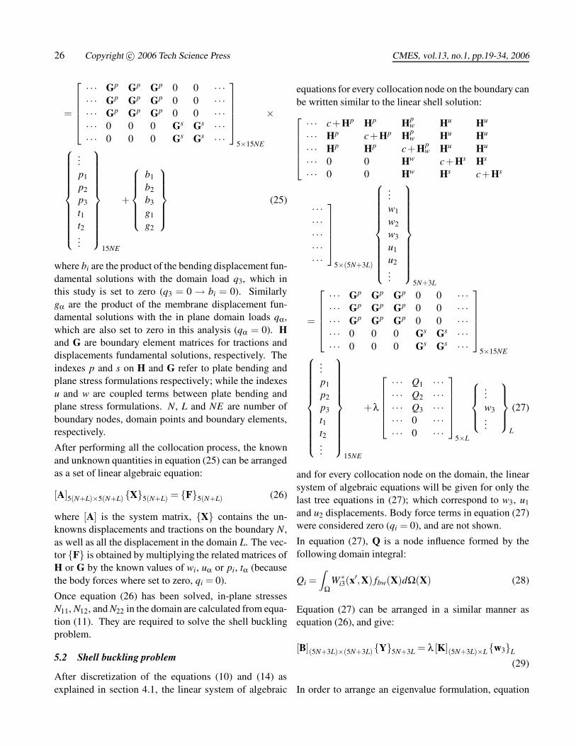
For axial compression of curved sheet panels (see figure2), the same method as in the case of a circular cylindri-cal tube axially compressed has been used for calculat-ing the critical stresses. The analytical solutions for anyof the buckling equations given so far in the literature,are based on the substitution of trigonometric functionswhich satisfy some specific boundary conditions and as-sumed buckling mode. On the other hand, they are basedon classical shell theory, where shear deformable effectsare not considered. Therefore, it seems more convenientto compare our results with finite element solutions.
Middle surface
h/2h/2
R
a
b
Nc
Nc
Figure 2 : Cylindrical shallow shell subjected to uniformaxial compression.
The buckling coefficients (K) and the curvature parame-ters (Z) for curved plate structures are defined as follows:
K =Ncr ·12(1−v2) ·b2
π2 ·E ·h2(34)
28 Copyright c© 2006 Tech Science Press CMES, vol.13, no.1, pp.19-34, 2006
and,
Z =b2 ·√1−v2
R ·h (35)
where Ncr represent the critical in plane stress, obtainedfrom the multiplication of the buckling factors λ withthe actual applied stress, and b denotes the length of thecurved side of the shell.
In the present work, two different sets of boundary condi-tions will be considered. The simply supported conditionrefers to zero out of plane displacement (w3 = 0) whilethe clamped condition is based on zero out of plane dis-placement and zero rotations (wi = 0). The in plane dis-placements in both cases were set free (uα �= 0). Theseboundary conditions are the same through all the bound-ary.
6.1 Convergency study
First of all, a convergency study was performed for thesimple supported case of a shallow shell subjected to uni-form axial compression, as shown in figure 2. The shellconsidered has an aspect ratio a/b = 2 and width b = 2in,thickness h = 0.03in, Young’s modulus E = 1.05 ·107psiand Poisson ratio v = 0.3. The radius of the shell isR = 6.5in that correspond for a curvature parameter ofZ = 19.568.
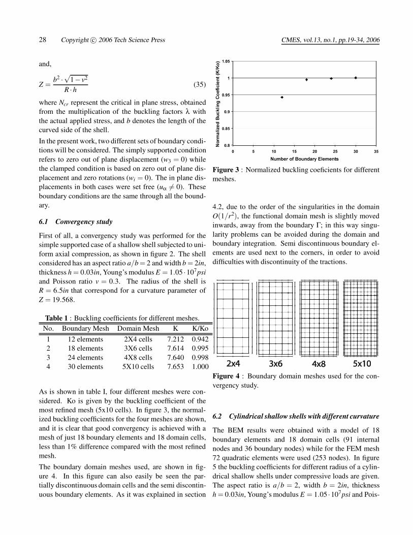
Table 1 : Buckling coefficients for different meshes.No. Boundary Mesh Domain Mesh K K/Ko
1 12 elements 2X4 cells 7.212 0.9422 18 elements 3X6 cells 7.614 0.9953 24 elements 4X8 cells 7.640 0.9984 30 elements 5X10 cells 7.653 1.000
As is shown in table I, four different meshes were con-sidered. Ko is given by the buckling coefficient of themost refined mesh (5x10 cells). In figure 3, the normal-ized buckling coefficients for the four meshes are shown,and it is clear that good convergency is achieved with amesh of just 18 boundary elements and 18 domain cells,less than 1% difference compared with the most refinedmesh.
The boundary domain meshes used, are shown in fig-ure 4. In this figure can also easily be seen the par-tially discontinuous domain cells and the semi discontin-uous boundary elements. As it was explained in section
Figure 3 : Normalized buckling coeficients for differentmeshes.
4.2, due to the order of the singularities in the domainO(1/r2), the functional domain mesh is slightly movedinwards, away from the boundary Γ; in this way singu-larity problems can be avoided during the domain andboundary integration. Semi discontinuous boundary el-ements are used next to the corners, in order to avoiddifficulties with discontinuity of the tractions.
Figure 4 : Boundary domain meshes used for the con-vergency study.
6.2 Cylindrical shallow shells with different curvature
The BEM results were obtained with a model of 18boundary elements and 18 domain cells (91 internalnodes and 36 boundary nodes) while for the FEM mesh72 quadratic elements were used (253 nodes). In figure5 the buckling coefficients for different radius of a cylin-drical shallow shells under compressive loads are given.The aspect ratio is a/b = 2, width b = 2in, thicknessh = 0.03in, Young’s modulus E = 1.05 ·107psi and Pois-
Linear Buckling Analysis 29
son ratio v = 0.3. As expected, an increase in the cur-vature also increase the buckling coefficients, while thedecrease of the curvature converge to the flat plate solu-tions.
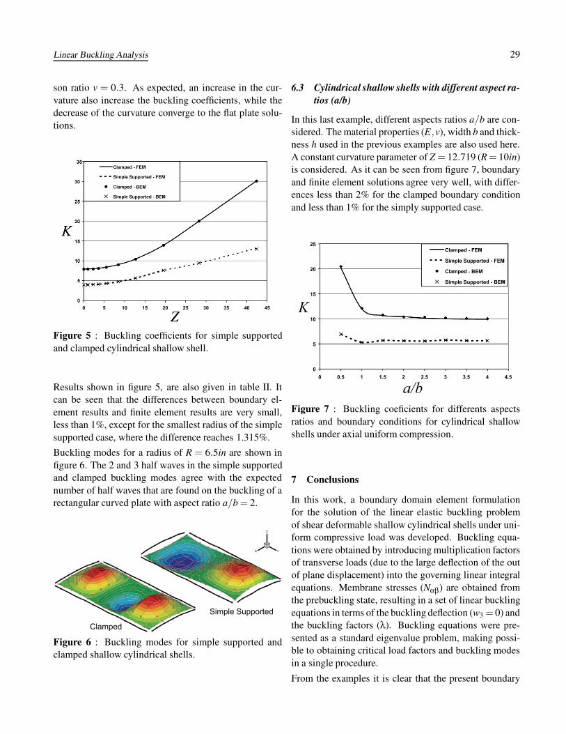
Figure 5 : Buckling coefficients for simple supportedand clamped cylindrical shallow shell.
Results shown in figure 5, are also given in table II. Itcan be seen that the differences between boundary el-ement results and finite element results are very small,less than 1%, except for the smallest radius of the simplesupported case, where the difference reaches 1.315%.
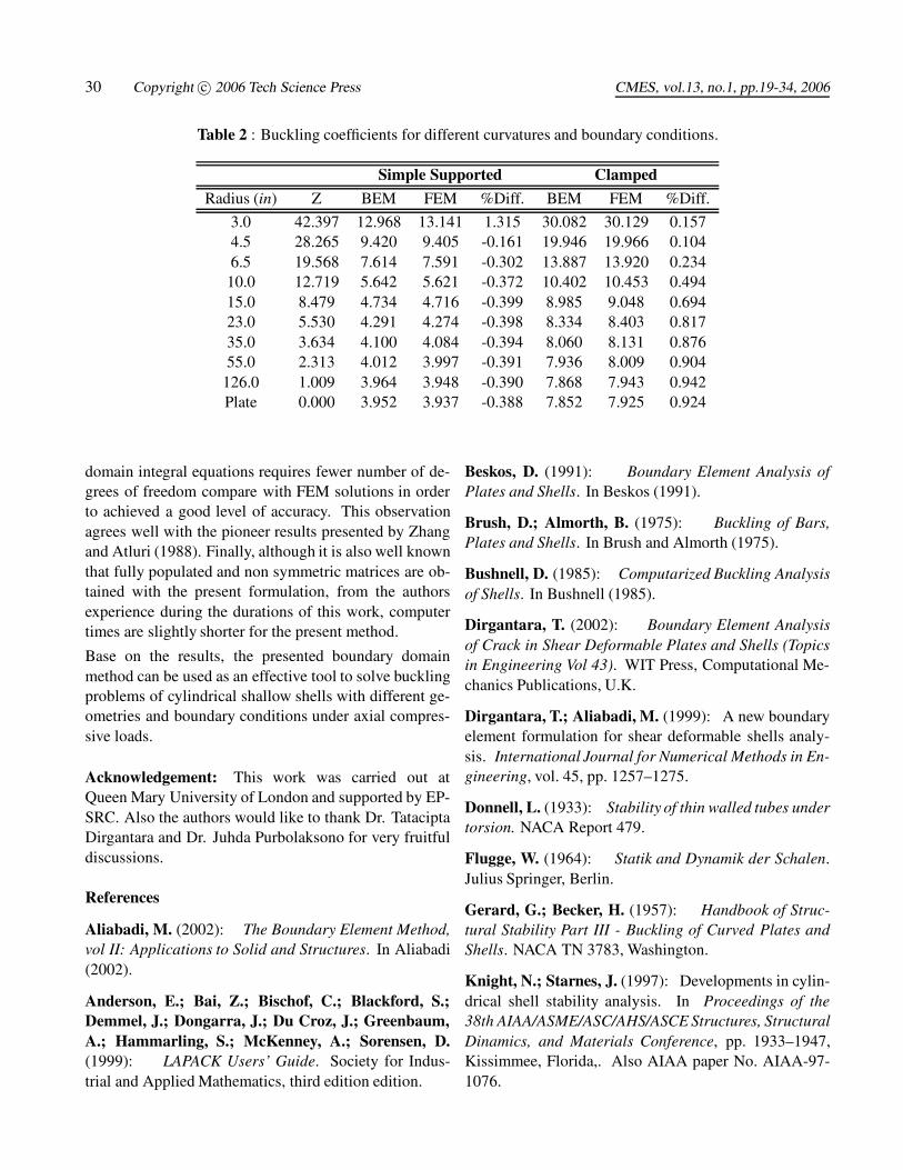
Buckling modes for a radius of R = 6.5in are shown infigure 6. The 2 and 3 half waves in the simple supportedand clamped buckling modes agree with the expectednumber of half waves that are found on the buckling of arectangular curved plate with aspect ratio a/b = 2.
Simple Supported
Clamped
Figure 6 : Buckling modes for simple supported andclamped shallow cylindrical shells.
6.3 Cylindrical shallow shells with different aspect ra-tios (a/b)
In this last example, different aspects ratios a/b are con-sidered. The material properties (E,v), width b and thick-ness h used in the previous examples are also used here.A constant curvature parameter of Z = 12.719 (R = 10in)is considered. As it can be seen from figure 7, boundaryand finite element solutions agree very well, with differ-ences less than 2% for the clamped boundary conditionand less than 1% for the simply supported case.
K
a/bFigure 7 : Buckling coeficients for differents aspectsratios and boundary conditions for cylindrical shallowshells under axial uniform compression.
7 Conclusions
In this work, a boundary domain element formulationfor the solution of the linear elastic buckling problemof shear deformable shallow cylindrical shells under uni-form compressive load was developed. Buckling equa-tions were obtained by introducing multiplication factorsof transverse loads (due to the large deflection of the outof plane displacement) into the governing linear integralequations. Membrane stresses (Nαβ) are obtained fromthe prebuckling state, resulting in a set of linear bucklingequations in terms of the buckling deflection (w3 = 0) andthe buckling factors (λ). Buckling equations were pre-sented as a standard eigenvalue problem, making possi-ble to obtaining critical load factors and buckling modesin a single procedure.
From the examples it is clear that the present boundary
30 Copyright c© 2006 Tech Science Press CMES, vol.13, no.1, pp.19-34, 2006
Table 2 : Buckling coefficients for different curvatures and boundary conditions.
Simple Supported Clamped
Radius (in) Z BEM FEM %Diff. BEM FEM %Diff.
3.0 42.397 12.968 13.141 1.315 30.082 30.129 0.1574.5 28.265 9.420 9.405 -0.161 19.946 19.966 0.1046.5 19.568 7.614 7.591 -0.302 13.887 13.920 0.23410.0 12.719 5.642 5.621 -0.372 10.402 10.453 0.49415.0 8.479 4.734 4.716 -0.399 8.985 9.048 0.69423.0 5.530 4.291 4.274 -0.398 8.334 8.403 0.81735.0 3.634 4.100 4.084 -0.394 8.060 8.131 0.87655.0 2.313 4.012 3.997 -0.391 7.936 8.009 0.904
126.0 1.009 3.964 3.948 -0.390 7.868 7.943 0.942Plate 0.000 3.952 3.937 -0.388 7.852 7.925 0.924
domain integral equations requires fewer number of de-grees of freedom compare with FEM solutions in orderto achieved a good level of accuracy. This observationagrees well with the pioneer results presented by Zhangand Atluri (1988). Finally, although it is also well knownthat fully populated and non symmetric matrices are ob-tained with the present formulation, from the authorsexperience during the durations of this work, computertimes are slightly shorter for the present method.
Base on the results, the presented boundary domainmethod can be used as an effective tool to solve bucklingproblems of cylindrical shallow shells with different ge-ometries and boundary conditions under axial compres-sive loads.
Acknowledgement: This work was carried out atQueen Mary University of London and supported by EP-SRC. Also the authors would like to thank Dr. TataciptaDirgantara and Dr. Juhda Purbolaksono for very fruitfuldiscussions.
References
Aliabadi, M. (2002): The Boundary Element Method,vol II: Applications to Solid and Structures. In Aliabadi(2002).
Anderson, E.; Bai, Z.; Bischof, C.; Blackford, S.;Demmel, J.; Dongarra, J.; Du Croz, J.; Greenbaum,A.; Hammarling, S.; McKenney, A.; Sorensen, D.(1999): LAPACK Users’ Guide. Society for Indus-trial and Applied Mathematics, third edition edition.
Beskos, D. (1991): Boundary Element Analysis ofPlates and Shells. In Beskos (1991).
Brush, D.; Almorth, B. (1975): Buckling of Bars,Plates and Shells. In Brush and Almorth (1975).
Bushnell, D. (1985): Computarized Buckling Analysisof Shells. In Bushnell (1985).
Dirgantara, T. (2002): Boundary Element Analysisof Crack in Shear Deformable Plates and Shells (Topicsin Engineering Vol 43). WIT Press, Computational Me-chanics Publications, U.K.
Dirgantara, T.; Aliabadi, M. (1999): A new boundaryelement formulation for shear deformable shells analy-sis. International Journal for Numerical Methods in En-gineering, vol. 45, pp. 1257–1275.
Donnell, L. (1933): Stability of thin walled tubes undertorsion. NACA Report 479.
Flugge, W. (1964): Statik and Dynamik der Schalen.Julius Springer, Berlin.
Gerard, G.; Becker, H. (1957): Handbook of Struc-tural Stability Part III - Buckling of Curved Plates andShells. NACA TN 3783, Washington.
Knight, N.; Starnes, J. (1997): Developments in cylin-drical shell stability analysis. In Proceedings of the38th AIAA/ASME/ASC/AHS/ASCE Structures, StructuralDinamics, and Materials Conference, pp. 1933–1947,Kissimmee, Florida,. Also AIAA paper No. AIAA-97-1076.
Linear Buckling Analysis 31
Leitao, V. (1994): Boundary Element in Nonlin-ear Fracture Mechanics (Topics in Engineering Vol 21).Computational Mechanics Publications, U.K.
Lin, J.; Duffield, R.; Shih, H. (1999): Boundary el-ement analysis of crack in shear deformable plates andshells (topics in engineering vol 43). Engineering Anal-ysis with Boundary Elements, vol. 23, pp. 131–137.
Manolis, G.; Beskos, D.; Pineros, M. (1986): Beamand plate stability by boundary elements. Computers &Structures, vol. 22, pp. 917–923.
Nash, W. (1966): Instability of Thin Shells. AppliedMechanics Survey. Spartan Books, Washintong D.C.
Nerantzaki, M.; Katsikadelis, J. (1996): Buckling ofplates with variable thickness - an analog equation so-lution. Engineering Analysis with Boundary Elements,vol. 18, pp. 149–154.
Noor, A. (1990): Bibliography of books and surveys onshells. Applied Mechanics Review, vol. 43, pp. 223–234.
O’Donoghue, P.; Atluri, S. (1987): Field/boundary el-ement approach to the large deflection of thin flat plates.Computers & Structures, vol. 27, pp. 427–435.
Purbolaksono, J.; Aliabadi, M. (2005): Buckling anal-ysis of shear deformable plates by the boundary elementmethod. International Journal for Numerical Methodsin Engineering, vol. 62, pp. 537–563.
Purbolaksono, J.; Aliabadi, M. (2005): Large defor-mation of shear deformable plates by the boundary ele-ment method. Journal of Engineering Mathematics, vol.51, pp. 211–230.
Purbolaksono, J.; Aliabadi, M. (2005): Dual Bound-ary Element Method for Instability Analysis of CrackedPlates. CMES: Computer Modeling in Engineering &Sciences, vol. 8, no. 1, pp. 73-90.
Reissner, E. (1947): On bending of elastic plates.Quarterly of Applied Mathematics, vol. 5, pp. 55–68.
Reissner, E. (1950): On a variational theorem in elas-ticity. Journal of Mathematics and Physics, vol. 29, pp.90–95.
Singer, J. (1982): Buckling experiments on shells - areview of recent developments. Solid Mechanics Arch,vol. 7, pp. 213–313.
Supriyono; Aliabadi, M. (2006): Boundary elementmethod for shear deformable plates with combined geo-metric and material nonlinearities. Engineering Analysiswith Boundary Elements, vol. 30, pp. 31–42.
Syngellakis, S.; Elzein, A. (1994): Plate bucklingloads by the boundary element method. InternationalJournal Numerical Method in Engineering, vol. 37, pp.1763–1778.
Telles, J. C. F. (1987): A self-adaptive coordinate trans-formation for efficient numerical evaluation of generalboundary element integrals. International Journal forNumerical Methods in Engineering, vol. 24, pp. 959–973.
Teng, G. (1996): Buckling of thin shells: Recent ad-vances and trends. Applied Mechanics Review, vol. 49,pp. 263–274.
Timoshenko, S.; Gere, J. (1961): Theory of ElasticStability. McGraw-Hill, New York, second edition edi-tion.
Vander Weeen, F. (1982): Application of the boundaryintegral equation method to reissner’s plate model. Inter-national Journal for Numerical Methods in Engineering,vol. 18, pp. 1–10.
Wen, P.; Aliabadi, M.; Young, A. (2006): Post-buckling analysis of shear deformable plates by bem.Journal of Strain Analysis for Engineering Design, vol.41.
Zhang, J.; Atluri, S. (1988): Post-buckling analysis ofshallow shells by the field-boundary element method. In-ternational Journal for Numerical Methods in Engineer-ing, vol. 26, pp. 571–587.
Appendix A: Appendix
The expressions for the kernels W ∗i j and P∗
i j are given byVander Weeen (1982) as follows:
W ∗αβ =
18πD(1−ν)
{[8B(z)− (1−ν)(2lnz−1)]δαβ
− [8A(z)+2(1−ν)]r,αr,β}W ∗
α3 = −W ∗3α =
18πD
(2lnz−1)rr,α
W ∗33 =
18πD(1−ν)λ2 [(1−ν)z2(lnz−1)−8lnz] (36)
32 Copyright c© 2006 Tech Science Press CMES, vol.13, no.1, pp.19-34, 2006
and
P∗γα =
−14πr
[(4A(z)+2zK1(z)+1−ν)(δαγr,n + r,αnγ)
+(4A(z)+1+ν)r,γnα
−2(8A(z)+2zK1(z)+1−ν)r,αr,γr,n]
P∗γ3 =
λ2
2π[B(z)nγ−A(z)r,γr,n]
P∗3α =
−(1−ν)8π
[(2(1+ν)(1−ν)
lnz−1
)nα +2r,αr,n
]
P∗33 =
−12πr
r,n (37)
where
A(z) = K0(z)+2z
[K1(z)− 1
z
]
B(z) = K0(z)+1z
[K1(z)− 1
z
](38)
in which K0(z) and K1(z) are modified Bessel functionsof the second kind, z = λr, r is the absolute distance be-tween the source and the field points, r,α = rα/r, whererα = xα(x)− xα(x′) and r,n = r,αnα.As it can be seen,A(z) is a smooth function, whereas, B(z) is a weakly sin-gular O(lnr). Therefore W ∗
i j is weakly singular and P∗i j
has a strong (Cauchy principal value) singularity O(1/r).
The expressions for the kernels U∗θα and T ∗
θα are thewell known (Kelvin solution) for two-dimensional planestress problems, and are given as Dirgantara and Aliabadi(1999) :
U∗θα =
14πB(1−ν)
[(3−ν) ln
(1r
)δθα +(1+ν) r,θr,α
](39)
T (i)∗θα = − 1
4πr{r,n [(1−ν)δθα +2(1+ν) r,θr,α]
+(1−ν) [nθr,α −nαr,θ]} (40)
where U∗θα are weakly singular kernels of order O
(ln
1r
)and T ∗
θα are strongly singular of order O(1/r) .
Derivatives of the displacement fundamental solutionswith respect to the field point (X) are given as follows:
W ∗γ3,α =
18πD
[(2lnz−1)δαγ +2r,γr,α
](41)
W ∗33,α =
r,α
8πD(1−ν)λ[z(1−ν)(2lnz−1)− 8
z] (42)
U∗αβ,γ =
1+v4πB(1−ν) r
×[−(3−ν)
(1+v)r,γδαβ +δαγr,β +δβγr,α −2r,βr,γr,α
](43)
The kernel W ∗γ3,α is regular, while W ∗
33,α and U∗αβ,γ are
weakly singular in the domain, singularity O(1/r).
The expressions for the kernels U∗αβγ and T ∗
αβγ are Dirgan-tara (2002):
U∗αβγ =
14πr
[(1−ν)
(δγαr,β +δγβr,α −δαβr,γ
)+2(1+ν) r,αr,βr,γ
](44)
T (i)∗αβγ =
B(1−ν)4πr2
{2r,n
[(1−ν)δαβr,γ
+ν(δγαr,β +δγβr,α
)−4(1+ν) r,αr,βr,γ]
+2ν(nαr,βr,γ +nβr,αr,γ
)+(1−ν)
(2nγr,αr,β +nβδαγ +nαδβγ
)−(1−3ν)nγδαβ
}(45)
Finally, the expression for U∗αβγ,θ is given by:
U∗αβγ,θ =
14πr2
{2(1+v)[δθαr,βr,γ +δβθr,αr,γ
+δθγr,βr,α −4r,αr,βr,γr,θ]−2r,θ (1−ν)
[δγαr,β +δγβr,α −δαβr,γ
]+(1−v)[δγαδβθ +δγβδαθ −δαβδγθ]
}(46)
Appendix B: Appendix
For the non curvature terms in equation (10), the differen-tiation can be applied directly to the tensors related to thefundamental solutions, whereas in the case of the curva-ture integral, which already have been differentiated once(U∗
θα,β), special considerations are necessary.
Let’s represent the curvature integral in equation (10) ona more formal manner:
Vθ = limε→0
ZΩε
U∗θα,β(X′,X)B
[kαβ (1−ν)+νδαβkφφ
]×w3(X)dΩ(X) (47)
where Ωε is the domain that remains after removed a cir-cle of radius ε centred at the point (X′) from the domainΩ.
Linear Buckling Analysis 33
The derivative of Vθ with respect to the coordinate xγ ofpoint (X′) can be written as:
∂Vθ
∂xγ= lim
ε→0
{∂
∂xγ
ZΩε
U∗θα,β(X′,X)B[
kαβ (1−ν)+νδαβkφφ]
w3(X)dΩ(X)}
(48)
The derivative of this domain integral, must be carriedout by using the Leibnitz formula, that is given by thefollowing expression:
ddα
Z ϕ2(α)
ϕ1(α)F(x,α)dx =
Z ϕ2(α)
ϕ1(α)
F(x,α)dα
dx
−F(ϕ(α),α)dϕ1(α)
dα+F(ϕ(α),α)
dϕ2(α)dα
(49)
After the Leibnitz formula have been applied to equation(48), one concludes that:
∂Vθ
∂xγ=
ZΩ−
U∗θα,β(X′,X)
∂xγB
[kαβ (1−ν)+νδαβkφφ
]×w3(X)dΩ(X)−B
[kαβ (1−ν)+νδαβkφφ
]w3(X′)×Z
Γ′U∗
θα,β(X′,x)r,γ dΓ′(x) (50)
where the first integral in the right hand side is in theCauchy principal value sense and the second one is cal-culated for a circle of radius ε → 0 centred at point (X′).
In order to solve the integral on Γ′, the following rela-tionships have to be considered:
r = ε; r,n = 1; dΓ′ = εdϕ
r,1 = cosϕ; r,2 = sinϕ
Now, it is possible to obtain the derivative of equation(10):
uθ(X′)∂γ
+Z
Γ− T ∗(i)
θα (X′,x)∂γ
uα(x)dΓ(x)
+Z
Ω−
U∗θα,β(X′,X)
∂xγB
[kαβ (1−ν)+νδαβkφφ
]×w3(X)dΩ(X)
− w3(X′)8(1−v)
{[kθγ (1−ν)+νδθγkφφ
](3v−5)
+[kθγ (v−1)+δθγkφφ
](1+v)
}=
ZΓ
U∗θα(X′,x)
∂γtα(x)dΓ(x)
+Z
Ω
U∗θα(X′,X)
∂γqα(X)dΩ(X) (51)
Finally, by introducing equation (51) into equation (6),the following expression can be obtained:
Nαβ(X′) =
ZΓ
U∗αβγ(X′,x)tγ(x)dΓ(x)
−Z
ΓT ∗
αβγ(X′,x)uγ(x)dΓ(x)
−Z
Ω− U∗
αβγ,θ(X′,X)B[kγθ (1−ν)+νδγθkφφ
]w3(X)dΩ(X)
+Z
ΩU∗
αβγ(X′,X)qγ(X)dΩ(X)
+B[(1−ν)kαβ +νδαβkφφ
]w3
(X′)
+Bw3 (X′)
8
{[kαβ (1−ν)+νδαβkφφ
](−v−5)
+[kαβ (ν−1)+δαβkφφ
](1−3v)
}(52)
Appendix C: Appendix
The quadratic continuous shape functions for the bound-ary are defined as:
Φ1(ξ) =12
ξ(ξ−1)
Φ2(ξ) = (1−ξ)(1+ξ)
Φ3(ξ) =12
ξ(ξ+1) (53)
For the case of semi-discontinuous boundary elements:
Φ1S1(ξ) =
910
ξ(ξ−1)
Φ1S3(ξ) =
610
ξ(
ξ− 23
)
Φ2S1(ξ) = −3
2(ξ−1)
(ξ+
23
)
Φ2S3(ξ) = −3
2(ξ+1)
(ξ− 2
3
)
Φ3S1(ξ) =
610
ξ(
ξ+23
)
Φ3S3(ξ) =
910
ξ(ξ+1) (54)
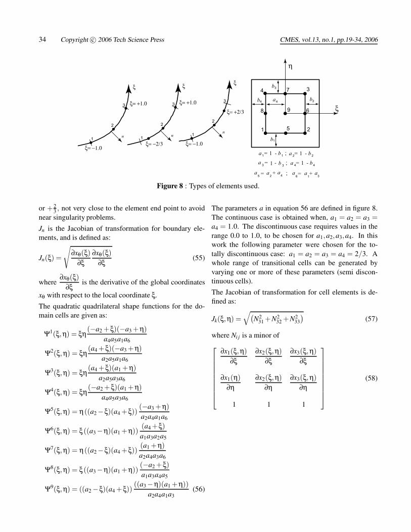
where ΦmS1 correspond to nodes placed at ξ = −2
3 ,0,+1,while Φm
S3 is for nodes placed at ξ = −1,0,+23 . See fig-
ure Appendix B:. The position of the internal node insemi-discontinuous element is chosen arbitrarily at −2
3
34 Copyright c© 2006 Tech Science Press CMES, vol.13, no.1, pp.19-34, 2006
1 2
34
5
6
7
8 9
a4b4
a = 1 - b ;
a12 345 6
1 1
η
ξ
b1
b3
b2
a = 1 - b2 2
;3 3 a = 1 - b4 4
ξ
1
2
3
n
ξ= +2/3
ξ= −1.0
ξ
1
2
3
n
ξ= +1.0
ξ= −2/3
ξ
1
2
3
n
ξ= +1.0
ξ= −1.0
a aa= +
a b
a a= +;
= 1 -
Figure 8 : Types of elements used.
or +23 , not very close to the element end point to avoid
near singularity problems.
Jn is the Jacobian of transformation for boundary ele-ments, and is defined as:
Jn(ξ) =
√∂xθ(ξ)
∂ξ∂xθ(ξ)
∂ξ(55)
where∂xθ(ξ)
∂ξis the derivative of the global coordinates
xθ with respect to the local coordinate ξ.
The quadratic quadrilateral shape functions for the do-main cells are given as:
Ψ1(ξ,η) = ξη(−a2 +ξ)(−a3 +η)
a4a5a1a6
Ψ2(ξ,η) = ξη(a4 +ξ)(−a3 +η)
a2a5a1a6
Ψ3(ξ,η) = ξη(a4 +ξ)(a1 +η)
a2a5a3a6
Ψ4(ξ,η) = ξη(−a2 +ξ)(a1 +η)
a4a5a3a6
Ψ5(ξ,η) = η((a2−ξ)(a4 +ξ))(−a3 +η)a2a4a1a6
Ψ6(ξ,η) = ξ((a3−η)(a1 +η))(a4 +ξ)a1a3a2a5
Ψ7(ξ,η) = η((a2−ξ)(a4 +ξ))(a1 +η)a2a4a3a6
Ψ8(ξ,η) = ξ((a3−η)(a1 +η))(−a2 +ξ)a1a3a4a5
Ψ9(ξ,η) = ((a2 −ξ)(a4 +ξ))((a3−η)(a1 +η))
a2a4a1a3(56)
The parameters a in equation 56 are defined in figure 8.The continuous case is obtained when, a1 = a2 = a3 =a4 = 1.0. The discontinuous case requires values in therange 0.0 to 1.0, to be chosen for a1,a2,a3,a4. In thiswork the following parameter were chosen for the to-tally discontinuous case: a1 = a2 = a3 = a4 = 2/3. Awhole range of transitional cells can be generated byvarying one or more of these parameters (semi discon-tinuous cells).
The Jacobian of transformation for cell elements is de-fined as:
Jk(ξ,η) =√(
N231 +N2
32 +N233
)(57)
where Ni j is a minor of⎡⎢⎢⎢⎢⎢⎢⎢⎢⎣
∂x1(ξ,η)∂ξ
∂x2(ξ,η)∂ξ
∂x3(ξ,η)∂ξ
∂x1(η)∂η
∂x2(ξ,η)∂η
∂x3(ξ,η)∂η
1 1 1
⎤⎥⎥⎥⎥⎥⎥⎥⎥⎦
(58)


![Development of deformable connection for earthquake ...static.tongtianta.site/paper_pdf/67ad414e-37ed-11e9-ab75-00163e08bb86.pdf · concrete building structures [17, 18]. Buckling](https://img.pdfslide.us/doc/110x75/5e80e9bfb9bb0676df55b3c1/development-of-deformable-connection-for-earthquake-concrete-building-structures.jpg)