Composite Structures 108 (2014) 341–353

Contents lists available at ScienceDirect

Composite Structures

journal homepage: www.elsevier .com/locate /compstruct

Wavelet spectral finite element for wave propagation in sheardeformable laminated composite plates

0263-8223/$ - see front matter � 2013 Elsevier Ltd. All rights reserved.http://dx.doi.org/10.1016/j.compstruct.2013.09.027

⇑ Corresponding author. Tel.: +1 662 325 3797; fax: +1 662 325 3864.E-mail addresses: dulip@raspet.msstate.edu (D. Samaratunga), jha@raspet.

msstate.edu (R. Jha), krishnan@aerospace.iisc.ernet.in (S. Gopalakrishnan).

Dulip Samaratunga a, Ratneshwar Jha a,⇑, S. Gopalakrishnan b

a Raspet Flight Research Laboratory, Mississippi State University, 114 Airport Road, Starkville, MS 39759, USAb Department of Aerospace Engineering, Indian Institute of Science, Bangalore 560 012, India

a r t i c l e i n f o

Article history:Available online 25 September 2013

Keywords:Wave propagationCompositeSpectral finite elementAbaqusShear deformation theoryStructural health monitoring

a b s t r a c t

This paper presents a new 2-D wavelet spectral finite element (WSFE) model for studying wave propa-gation in thin to moderately thick anisotropic composite laminates. The WSFE formulation is based onthe first order shear deformation theory (FSDT) which yields accurate results for wave motion at high fre-quencies. The wave equations are reduced to ordinary differential equations (ODEs) using Daubechiescompactly supported, orthonormal, scaling functions for approximations in time and one spatial dimen-sion. The ODEs are decoupled through an eigenvalue analysis and then solved exactly to obtain the shapefunctions used in element formulation. The developed spectral element captures the exact inertial distri-bution, hence a single element is sufficient to model a laminate of any dimension in the absence of dis-continuities. The 2-D WSFE model is highly efficient computationally and provides a direct relationshipbetween system input and output in the frequency domain. Results for axial and transverse wave prop-agations in laminated composite plates of various configurations show excellent agreement with finiteelement simulations using Abaqus�.

� 2013 Elsevier Ltd. All rights reserved.

1. Introduction

Wave propagation in elastic structures has been studied exten-sively and applied for transient response prediction, mechanicalproperty characterization, and nondestructive evaluation (NDE)[1–5]. Composite (elastic) structures are increasingly used in manyindustries such as transportation (air, land, and sea), wind energy,and civil infrastructure due to several advantages including higherspecific strength and modulus, fewer joints, improved fatigue life,and higher resistance to corrosion. Lamb wave based structuralhealth monitoring (SHM), which aims to perform nondestructiveevaluation through integrated actuators and sensors, has been avery active area of research in the past decade [6–10]. A validatedphysics-based model for wave propagation combined with exper-imental measurements is generally required for complete charac-terization (presence, location, and severity) of damages.

The modeling of wave propagation in composites presents com-plexities beyond that for isotropic structures [2,4]. Analytical solu-tions for wave propagation are not available for most practicalstructures due to complex nature of governing differential equa-tions and boundary/initial conditions. The finite element method(FEM) is the most popular numerical technique for modeling wave

propagation phenomena. However, for accurate predictions usingFEM, typically 20 elements should span a wavelength [11], whichresults in very large system size and enormous computational costfor wave propagation analysis at high frequencies. In addition,solving inverse problems (as required for NDE/SHM) is very diffi-cult using FEM. Spectral finite element (SFE), which follows FEMmodeling procedure in the transformed frequency domain, ishighly suitable for wave propagation analysis [12–14]. SFE modelsare many orders smaller than FEM and highly suitable for efficientNDE/SHM. Frequency domain formulation of SFE enables directrelationship between output and input through system transferfunction (frequency response function). SFE has very high compu-tational efficiency since nodal displacements are related to nodaltractions through frequency-wave number dependent stiffnessmatrix. Mass distribution is captured exactly and the accurate ele-mental dynamic stiffness matrix is derived. Consequently, in theabsence of any discontinuities, one element is sufficient to modela beam or plate structure of any length.

Fast Fourier Transform (FFT) based Spectral Finite Element(FSFE) method was popularized by Doyle [12], who formulatedFSFE models for isotropic 1-D and 2-D waveguides including ele-mentary rod, Euler Bernoulli beam, and thin plate. Gopalakrishnanand associates [13,15] extensively investigated FSFE models forbeams and plates-with anisotropic and inhomogeneous materialproperties. The FSFE method is very efficient for wave motion anal-ysis and it is suitable for solving inverse problems; however, FSFE

342 D. Samaratunga et al. / Composite Structures 108 (2014) 341–353

cannot model waveguides of short lengths. For 2-D problems, FSFEare essentially semi-infinite, that is, they are bounded only in onedirection [12,13]. Due to the global basis functions of the Fourierseries approximation of the spatial dimension, the effect of lateralboundaries cannot be captured. In addition, FSFE requires assump-tion of periodicity in time approximation resulting in ‘‘wrap-around’’ problem for smaller time window, which totally distortsthe response.

The 2-D Wavelet based Spectral Finite Element (WSFE) pre-sented by Gopalakrishnan and Mitra [14] overcomes the ‘‘wrap-around’’ problem and can accurately model 2-D plate structuresof finite dimensions. WSFE uses orthogonal compactly supported(localized) Daubechies scaling functions [16] as basis for both tem-poral and spatial approximations. Gopalakrishnan and associateshave formulated WSFE elements for wave propagation in rods,higher order beams, and plates with both isotropic and anisotropicmaterial properties [17–20]. However, the 2-D WSFE plate formu-lation presented in [14,19,20] is based on the classical laminatedplate theory (CLPT) [21]. The CLPT based formulations excludetransverse shear deformation and rotary inertia resulting in signifi-cant errors for wave motion analysis at high frequencies, especiallyfor composite laminates which have relatively low transverse shearmodulus [22,23]. Wave propagation in composite laminates basedon the first order shear deformation theory (FSDT) [21], which ac-counts for transverse shear and rotary inertia, yields accurately re-sults comparable with 3-D elasticity solutions and experimentseven at high frequencies [22,23]. For isotropic materials FSDT isknown to be exceptionally accurate down to wavelengths compara-ble with the plate thickness h, whereas CLPT is of acceptable accu-racy only for wavelengths greater than, say, 20h [24].

This paper presents a new 2-D WSFE based on FSDT for high fre-quency analysis of waveguides with finite dimensions and aniso-tropic material properties. Governing partial differential equations(PDEs) for wave motion and their temporal approximation usingDaubechies compactly supported high-order scaling functions arepresented. An eigenvalue analysis is performed to decouple the re-duced PDEs in spatial dimensions. The decoupled PDEs are thenapproximated in one spatial dimension using Daubechies lower-or-der scaling functions followed by an eigenvalue analysis similar tothe time approximation. The resulting ordinary differential equa-tions (ODEs) are solved exactly in frequency-wavenumber domainand the solution is used as shape function for the 2-D spectral ele-ment. Numerical experiments are performed to highlight the differ-ences between FSDT and CLPT in dispersion curves, providespectrum relationships, and present time domain responses. Resultsfor the new WSFE formulation are validated with Abaqus� simula-tions using shear flexible shell elements [25].

2. Formulation of wavelet spectral finite element with sheardeformation

Two dimensional wavelet spectral finite element with sheardeformation is formulated here for anisotropic compositelaminates.

2.1. Governing differential equations for wave propagation

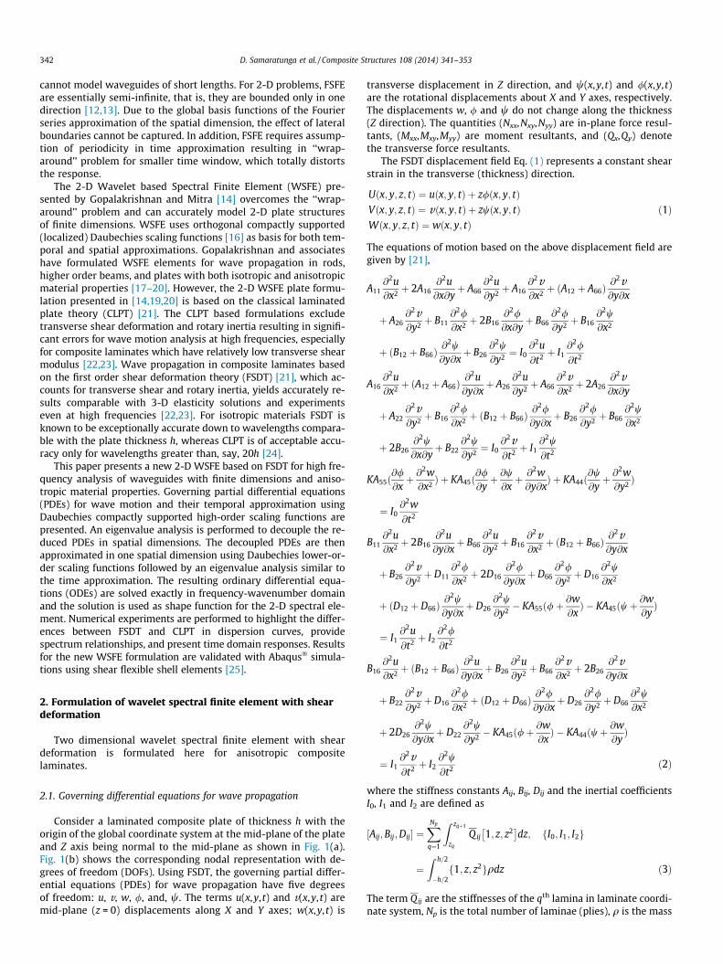
Consider a laminated composite plate of thickness h with theorigin of the global coordinate system at the mid-plane of the plateand Z axis being normal to the mid-plane as shown in Fig. 1(a).Fig. 1(b) shows the corresponding nodal representation with de-grees of freedom (DOFs). Using FSDT, the governing partial differ-ential equations (PDEs) for wave propagation have five degreesof freedom: u, v, w, /, and, w. The terms u(x,y, t) and v(x,y, t) aremid-plane (z = 0) displacements along X and Y axes; w(x,y, t) is

transverse displacement in Z direction, and w(x,y, t) and /(x,y, t)are the rotational displacements about X and Y axes, respectively.The displacements w, / and w do not change along the thickness(Z direction). The quantities (Nxx,Nxy,Nyy) are in-plane force resul-tants, (Mxx,Mxy,Myy) are moment resultants, and (Qx,Qy) denotethe transverse force resultants.

The FSDT displacement field Eq. (1) represents a constant shearstrain in the transverse (thickness) direction.

Uðx; y; z; tÞ ¼ uðx; y; tÞ þ z/ðx; y; tÞVðx; y; z; tÞ ¼ vðx; y; tÞ þ zwðx; y; tÞWðx; y; z; tÞ ¼ wðx; y; tÞ

ð1Þ

The equations of motion based on the above displacement field aregiven by [21],

A11@2u@x2 þ 2A16

@2u@x@y

þ A66@2u@y2 þ A16

@2v@x2 þ ðA12 þ A66Þ

@2v@y@x

þ A26@2v@y2 þ B11

@2/@x2 þ 2B16

@2/@x@y

þ B66@2/@y2 þ B16

@2w@x2

þ ðB12 þ B66Þ@2w@y@x

þ B26@2w@y2 ¼ I0

@2u@t2 þ I1

@2/

@t2

A16@2u@x2 þ ðA12 þ A66Þ

@2u@y@x

þ A26@2u@y2 þ A66

@2v@x2 þ 2A26

@2v@x@y

þ A22@2v@y2 þ B16

@2/@x2 þ ðB12 þ B66Þ

@2/@y@x

þ B26@2/@y2 þ B66

@2w@x2

þ 2B26@2w@x@y

þ B22@2w@y2 ¼ I0

@2v@t2 þ I1

@2w

@t2

KA55ð@/@xþ @

2w@x2 Þ þ KA45ð

@/@yþ @w@xþ @2w@y@x

Þ þ KA44ð@w@yþ @

2w@y2 Þ

¼ I0@2w@t2

B11@2u@x2 þ 2B16

@2u@y@x

þ B66@2u@y2 þ B16

@2v@x2 þ ðB12 þ B66Þ

@2v@y@x

þ B26@2v@y2 þ D11

@2/@x2 þ 2D16

@2/@y@x

þ D66@2/@y2 þ D16

@2w@x2

þ ðD12 þ D66Þ@2w@y@x

þ D26@2w@y2 � KA55ð/þ

@w@xÞ � KA45ðwþ

@w@yÞ

¼ I1@2u@t2 þ I2

@2/

@t2

B16@2u@x2 þ ðB12 þ B66Þ

@2u@y@x

þ B26@2u@y2 þ B66

@2v@x2 þ 2B26

@2v@y@x

þ B22@2v@y2 þ D16

@2/@x2 þ ðD12 þ D66Þ

@2/@y@x

þ D26@2/@y2 þ D66

@2w@x2

þ 2D26@2w@y@x

þ D22@2w@y2 � KA45ð/þ

@w@xÞ � KA44ðwþ

@w@yÞ

¼ I1@2v@t2 þ I2

@2w

@t2 ð2Þ

where the stiffness constants Aij, Bij, Dij and the inertial coefficientsI0, I1 and I2 are defined as

½Aij;Bij;Dij� ¼XNp

q¼1

Z zqþ1

zq

Q ij 1; z; z2� �

dz; I0; I1; I2f g

¼Z h=2

�h=2f1; z; z2gqdz ð3Þ

The term Qij are the stiffnesses of the qth lamina in laminate coordi-nate system, Np is the total number of laminae (plies), q is the mass

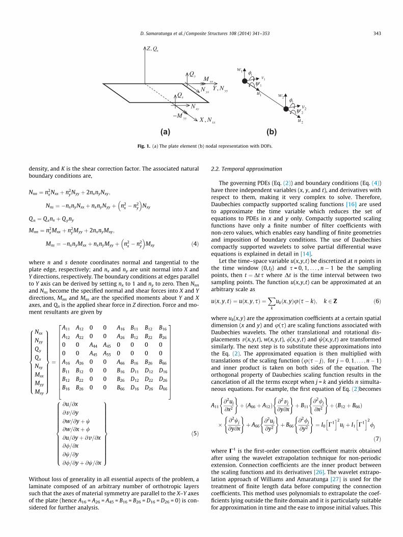
(a) (b)Fig. 1. (a) The plate element (b) nodal representation with DOFs.

D. Samaratunga et al. / Composite Structures 108 (2014) 341–353 343

density, and K is the shear correction factor. The associated naturalboundary conditions are,

Nnn ¼ n2x Nxx þ n2

y Nyy þ 2nxnyNxy;

Nns ¼ �nxnyNxx þ nxnyNyy þ n2x � n2

y

� �Nxy

Q n ¼ Q xnx þ Q yny

Mnn ¼ n2x Mxx þ n2

yMyy þ 2nxnyMxy;

Mns ¼ �nxnyMxx þ nxnyMyy þ n2x � n2

y

� �Mxy ð4Þ

where n and s denote coordinates normal and tangential to theplate edge, respectively; and nx and ny are unit normal into X andY directions, respectively. The boundary conditions at edges parallelto Y axis can be derived by setting nx to 1 and ny to zero. Then Nnn

and Nns become the specified normal and shear forces into X and Ydirections, Mnn and Mns are the specified moments about Y and Xaxes, and Qn is the applied shear force in Z direction. Force and mo-ment resultants are given by

Nxx

Nyy

Qy

Qx

Nxy

Mxx

Myy

Mxy

8>>>>>>>>>>>>><>>>>>>>>>>>>>:

9>>>>>>>>>>>>>=>>>>>>>>>>>>>;¼

A11 A12 0 0 A16 B11 B12 B16

A12 A22 0 0 A26 B12 B22 B26

0 0 A44 A45 0 0 0 00 0 A45 A55 0 0 0 0A16 A26 0 0 A66 B16 B26 B66

B11 B12 0 0 B16 D11 D12 D16

B12 B22 0 0 B26 D12 D22 D26

B16 B26 0 0 B66 D16 D26 D66

266666666666666664

377777777777777775@u=@x

@v=@y

@w=@yþ w

@w=@xþ /

@u=@yþ @v=@x@/=@x

@w=@y

@/=@yþ @w=@x

8>>>>>>>>>>>>><>>>>>>>>>>>>>:

9>>>>>>>>>>>>>=>>>>>>>>>>>>>;ð5Þ

Without loss of generality in all essential aspects of the problem, alaminate composed of an arbitrary number of orthotropic layerssuch that the axes of material symmetry are parallel to the X–Y axesof the plate (hence A16 = A26 = A45 = B16 = B26 = D16 = D26 = 0) is con-sidered for further analysis.

2.2. Temporal approximation

The governing PDEs (Eq. (2)) and boundary conditions (Eq. (4))have three independent variables (x, y, and t), and derivatives withrespect to them, making it very complex to solve. Therefore,Daubechies compactly supported scaling functions [16] are usedto approximate the time variable which reduces the set ofequations to PDEs in x and y only. Compactly supported scalingfunctions have only a finite number of filter coefficients withnon-zero values, which enables easy handling of finite geometriesand imposition of boundary conditions. The use of Daubechiescompactly supported wavelets to solve partial differential waveequations is explained in detail in [14].

Let the time–space variable u(x,y, t) be discretized at n points inthe time window (0, tf) and s = 0, 1, . . . , n � 1 be the samplingpoints, then t ¼ Dts where Dt is the time interval between twosampling points. The function u(x,y, t) can be approximated at anarbitrary scale as

uðx; y; tÞ ¼ uðx; y; sÞ ¼X

k

ukðx; yÞuðs� kÞ; k 2 Z ð6Þ

where uk(x,y) are the approximation coefficients at a certain spatialdimension (x and y) and u(s) are scaling functions associated withDaubechies wavelets. The other translational and rotational dis-placements v (x,y, t), w(x,y, t), /(x,y, t) and w(x,y, t) are transformedsimilarly. The next step is to substitute these approximations intothe Eq. (2). The approximated equation is then multiplied withtranslations of the scaling function (uðs� jÞ; for j ¼ 0;1; . . . ;n� 1)and inner product is taken on both sides of the equation. Theorthogonal property of Daubechies scaling function results in thecancelation of all the terms except when j = k and yields n simulta-neous equations. For example, the first equation of Eq. (2)becomes

A11@2uj

@x2

( )þ ðA66 þ A12Þ

@2v j

@y@x

( )þ B11

@2/j

@x2

( )þ ðB12 þ B66Þ

�@2wj

@y@x

( )þ A66

@2uj

@y2

( )þ B66

@2/j

@y2

( )¼ I0 C1

h i2uj þ I1 C1

h i2/j

ð7Þ

where C1 is the first-order connection coefficient matrix obtainedafter using the wavelet extrapolation technique for non-periodicextension. Connection coefficients are the inner product betweenthe scaling functions and its derivatives [26]. The wavelet extrapo-lation approach of Williams and Amaratunga [27] is used for thetreatment of finite length data before computing the connectioncoefficients. This method uses polynomials to extrapolate the coef-ficients lying outside the finite domain and it is particularly suitablefor approximation in time and the ease to impose initial values. This

344 D. Samaratunga et al. / Composite Structures 108 (2014) 341–353

extrapolation technique addresses one of the serious problems withFourier based SFE method, namely, the ‘wraparound’ problemcaused by treating the boundaries as periodic extensions. By solvingthe ‘wraparound’ problem, WSFE method is able to handle shortwaveguides and smaller time windows efficiently. Next, the cou-pled PDEs are decoupled using eigenvalue analysis of C1 followingthe procedure in [14]. The final decoupled form of the reduced PDEsgiven in Eq. (7) can be written as

A11@2uj

@x2 þ ðA66 þ A12Þ@2v j

@y@xþ B11

@2/j

@x2 þ ðB12 þ B66Þ@2wj

@y@xþ A66

@2uj

@y2

þ B66@2/j

@y2 ¼ �I0c2j uj � I1c2

j /j; j ¼ 0;1; . . . ;n� 1 ð8Þ

where uj is given by uj ¼ U�1uj, U is the eigenvector matrix of C1

and icjði ¼ffiffiffiffiffiffiffi�1p

Þ are the corresponding eigenvalues. Following ex-actly similar steps, the other four governing PDEs (in Eq. (2)) andthe natural boundary conditions (Eq. (4)) are transformed to PDEsin spatial dimensions (x and y) only. It should be mentioned herethat the sampling rate Dt should be less than a certain value toavoid spurious dispersion in the simulation using WSFE. In Mitraand Gopalakrishnan [14], a numerical study has been conductedfrom which the required Dt can be determined depending on theorder N of the Daubechies scaling function and frequency contentof the load.

2.3. Spatial (Y) approximation

The next step is to further reduce each of the transformed anddecoupled PDEs given by Eq. (8)(and similarly for the other trans-formed governing equations and boundary conditions) to a set ofcoupled ODEs using Daubechies scaling function approximationin one of the spatial (Y) dimension. Similar to time approximation,the time transformed variable uj is discretized at m points in thespatial window (0, LY), where LY is the length in Y direction. Letf = 0, 1, . . . , m � 1 be the sampling points, then y = DYf where DYis the spatial interval between two sampling points.

The function uj can be approximated by scaling function u(f) atan arbitrary scale as

ujðx; yÞ ¼ ujðx; fÞ ¼X

l

uljðxÞuðf� lÞ; l 2 Z ð9Þ

where ulj are the approximation coefficients at a certain spatialdimension x. The other four displacements v jðx; yÞ; wjðx; yÞ;/jðx; yÞ; and wjðx; yÞ are similarly transformed. Following similarsteps as the time approximation, substituting the above approxima-tions in Eq. (8)and taking inner product on both sides with thetranslates of scaling functions u(f � i), where i = 0, 1, . . . , m � 1and using their orthogonality property (which results in the cancel-ation of all the terms except when i = l), we get m simultaneousODEs. For example, the first of the Eq. (2), which is temporallyreduced in Eq. (8), can be spatially reduced as

A11d2uij

dx2 þ ðA66 þ A12Þ1

DY

Xl¼iþN�2

l¼i�Nþ2

dv lj

dxX1

i�l

þ ðB12 þ B66Þ1

DY

Xl¼iþN�2

l¼i�Nþ2

dwlj

dxX1

i�l þ B11d2/ij

dx2

þ A661

DY2

Xl¼iþN�2

l¼i�Nþ2

uljX2i�l þ B66

1DY2

Xl¼iþN�2

l¼i�Nþ2

/ljX2i�l

¼ �I0c2j uij � I1c2

j /ij ð10Þ

where N is the order of Daubechies wavelet and X1i�l and X2

i�l are theconnection coefficients for first- and second-order derivatives [26].

It can be seen from the ODEs given by Eq. (10) that similar totime approximation, even here certain coefficients uij near thevicinity of the boundaries (i = 0 and i = m�1) lie outside the spatialwindow (0,LY) defined by i = 0, 1, . . . , m � 1. These coefficientsmust be treated properly for finite domain analysis. Unlike timeapproximation, these coefficients are obtained through periodicextension for free lateral edges, while other boundary conditionsmay be imposed using a restraint matrix [14]. In the present study,the lateral boundaries are unrestrained (free–free) and boundaryconditions have been imposed using periodic extension. In addi-tion, it allows decoupling of the ODEs using eigenvalue analysisand thus reduces the computational cost. Here, after expressingthe unknown coefficients lying outside the finite domain interms of the inner coefficients considering periodic extension, theODEs given by Eq. (10) can be written as a matrix equation ofthe form as

A11d2uij

dx2

( )þ ðA66 þ A12Þ½K1� dv ij

dx

� �þ B11

d2/ij

dx2 þ ðB12 þ B66Þ½K1�

dwij

dx

( )þ A66½K1�

2fuijg þ B66½K1�

2/ij

n o¼ �I0c2

j fuijg � I1c2j /ij

n oð11Þ

where K1 is the first-order connection coefficient matrix obtainedafter periodic extension.

The coupled ODEs given by Eq. (11) are decoupled usingeigenvalue analysis similar to that done in temporal approxi-mation. It should be mentioned here that matrix K1 obtainedafter periodic extension has a circulant form and its eigenparameters are known analytically [14]. Let the eigenvaluesbe ibiði ¼

ffiffiffiffiffiffiffi�1p

Þ, then the decoupled ODEs corresponding toEq. (11) are given by

A11d2~uij

dx2 � ibiðA66 þ A12Þd~v ij

dxþ B11

d2 ~/ij

dx2 � ibiðB12 þ B66Þd~wij

dx

� b2i A66~uij � b2

i B66~/ij ¼ �I0c2

j~uij � I1c2

j~/ij ð12Þ

where ~uij (and similarly other transformed displacements) are givenby ~uij ¼ W�1uij; W is the eigenvector and ibi are the eigenvalues ofconnection coefficient matrix K1. Exactly the same procedure is fol-lowed to obtain decoupled form of the other four ODEs in Eq. (2) toobtain

A66d2 ~v ij

dx2 þ B66d2 ~wij

dx2 � ibiðA66 þ A12Þd~uij

dx� b2

i A22 ~v ij � ibiðB66 þ B12Þd~/ij

dx

� b2i B22

~wij ¼ �c2j I0 ~v ij � c2

j I1~wij

KA55d2 ~wij

dx2 þd~/ij

dx

!� KA44 b2

i~wij þ ibi

~wij

� �¼ �c2

j I0 ~wij

B11d2~uij

dx2 � ibiðB66 þ B12Þd~v ij

dxþ D11

d~/ij

dx2 � ibiðD66 þ D12Þd~wij

dx

� b2i B66~uij � b2

i D66~/ij � KA55

d ~wij

dxþ ~/ij

¼ �c2

j I2~/ij � c2

j I1~uij

B66d2 ~v ij

dx2 þ D66d2 ~wij

dx2 � ibiðB66 þ B12Þd~uij

dx� b2

i B22 ~v ij � ibiðD66 þ D12Þd~/ij

dx

� b2i D22

~wij � KA44 �ibi ~wij þ ~wij

� �¼ �c2

j I2~wij � c2

j I1 ~v ij

ð13Þ

The natural boundary conditions (Eq. (4)) after temporal and spatialapproximations are given as

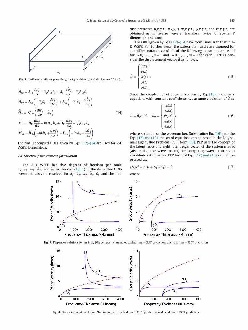
Fig. 2. Uniform cantilever plate (length = LX, width = LY, and thickness = 0.01 m).

D. Samaratunga et al. / Composite Structures 108 (2014) 341–353 345

eNxx ¼ A11d~uij

dx� ibiA12 ~v ij þ B11

d~/ij

dx� ibiB12

~wij

eNxy ¼ A66 �ibi~uij þd~v ij

dx

þ B66 �ibi

~/ij þd~wij

dx

!eQ x ¼ KA55

d ~wij

dxþ ~/ij

fMxx ¼ B11

d~uij

dx� ibiB12 ~v ij þ D11

d~/ij

dx� ibiD12

~wij

fMxy ¼ B66 �ibi~uij þd~v ij

dx

þ D66 �ibi

~/ij þd~wij

dx

!ð14Þ

The final decoupled ODEs given by Eqs. (12)–(14)are used for 2-DWSFE formulation.

2.4. Spectral finite element formulation

The 2-D WSFE has five degrees of freedom per node,uij; ~v ij; ~wij; ~/ij; and ~wij, as shown in Fig. 1(b). The decoupled ODEspresented above are solved for uij; ~v ij; ~wij; ~/ij; ~wij and the final

Fig. 3. Dispersion relations for an 8-ply [0]8 composite laminate; d

Fig. 4. Dispersion relations for an Aluminum plate; dashed l

displacements u(x,y, t), v(x,y, t), w(x,y, t), /(x,y, t) and w(x,y, t) areobtained using inverse wavelet transform twice for spatial Ydimension and time.

The ODEs given by Eqs. (12)–(14)have forms similar to that in 1-D WSFE. For further steps, the subscripts j and i are dropped forsimplified notations and all of the following equations are validfor j = 0, 1, . . . , n � 1 and i = 0, 1, . . . , m � 1 for each j. Let us con-sider the displacement vector ~d as follows,

~d ¼

~uðxÞ~vðxÞ~wðxÞ~/ðxÞ~wðxÞ

8>>>>>><>>>>>>:

9>>>>>>=>>>>>>;ð15Þ

Since the coupled set of equations given by Eq. (13) is ordinaryequations with constant coefficients, we assume a solution of ~d as

~d ¼ ~d0e�ijx; ~d0 ¼

~u0ðxÞ~v0ðxÞ~w0ðxÞ~/0ðxÞ~w0ðxÞ

8>>>>>><>>>>>>:

9>>>>>>=>>>>>>;ð16Þ

where j stands for the wavenumber. Substituting Eq. (16) into theEqs. (12) and (13), the set of equations can be posed in the Polyno-mial Eigenvalue Problem (PEP) form [13]. PEP uses the concept ofthe latent roots and right latent eigenvector of the system matrix(also called the wave matrix) for computing wavenumber andamplitude ratio matrix. PEP form of Eqs. (12) and (13) can be ex-pressed as,

fA2j2 þ A1jþ A0gf~d0g ¼ 0 ð17Þ

where

ashed line – CLPT prediction, and solid line – FSDT prediction.

ine – CLPT prediction, and solid line – FSDT prediction.

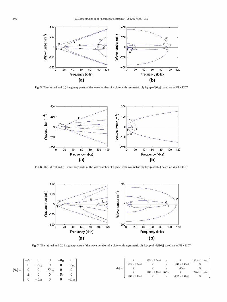
Fig. 5. The (a) real and (b) imaginary parts of the wavenumber of a plate with symmetric ply layup of [010] based on WSFE + FSDT.

Fig. 6. The (a) real and (b) imaginary parts of the wavenumber of a plate with symmetric ply layup of [010] based on WSFE + CLPT.

Fig. 7. The (a) real and (b) imaginary parts of the wave number of a plate with asymmetric ply layup of [05/905] based on WSFE + FSDT.

346 D. Samaratunga et al. / Composite Structures 108 (2014) 341–353

½A2� ¼

�A11 0 0 �B11 00 �A66 0 0 �B66

0 0 �KA55 0 0�B11 0 0 �D11 0

0 �B66 0 0 �D66

26666664

37777775

½A1� ¼

0 �bðA12 þ A66Þ 0 0 �bðB12 þ B66Þ�bðA12 þ A66Þ 0 0 �bðB12 þ B66Þ 0

0 0 0 �iKA55 00 �bðB12 þ B66Þ iKA55 0 �bðD12 þ D66Þ

�bðB12 þ B66Þ 0 0 �bðD12 þ D66Þ 0

26666664

37777775

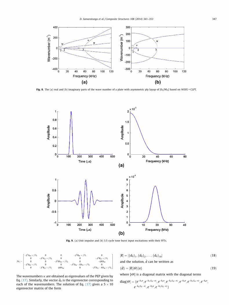
Fig. 8. The (a) real and (b) imaginary parts of the wave number of a plate with asymmetric ply layup of [05/905] based on WSFE + CLPT.

Fig. 9. (a) Unit impulse and (b) 3.5 cycle tone burst input excitations with their FFTs.

D. Samaratunga et al. / Composite Structures 108 (2014) 341–353 347

½A0 � ¼

�b2A66 þ c2 I0 0 0 �b2B66 þ c2I1 00 �b2A22 þ c2I0 0 0 �b2B22 þ c2I1

0 0 �b2KA44 þ c2I0 0 �ibKA44

�b2B66 þ c2I1 0 0 �b2D66 � KA55 þ c2I2 00 �b2B22 þ c2I1 ibKA44 0 �b2D22 � KA44 þ c2 I2

26666664

37777775

The wavenumbers j are obtained as eigenvalues of the PEP given byEq. (17). Similarly, the vector ~d0 is the eigenvector corresponding toeach of the wavenumbers. The solution of Eq. (17) gives a 5 � 10eigenvector matrix of the form

½R� ¼ ½fd0g1; fd0g2; . . . ; fd0g10� ð18Þ

and the solution, ~d can be written as

f~dg ¼ ½R�½H�fag ð19Þ

where [H] is a diagonal matrix with the diagonal terms

diag½H� ¼ fe�k1x; e�k1ðLX�xÞ; e�k2x; e�k2ðLX�xÞ; e�k3x; e�k3ðLX�xÞ; e�k4x;

e�k4ðLX�xÞ; e�k5x; e�k5ðLX�xÞg

348 D. Samaratunga et al. / Composite Structures 108 (2014) 341–353

Here, {a}T = {C1, C2, . . . , C10} are the unknown coefficients which canbe determined as described later. Since the procedure beyond thisstep is similar to the 2-D FSFE technique [12], it is not repeated

here. Finally, the transformed nodal forces fF�

eg and transformed no-

dal displacements fu�

eg are related by

fF�

eg ¼ ½K�

e�fu�eg ð20Þ

where ½K�

e� is the exact elemental dynamic stiffness matrix. Thesolution of Eq. (20) and the assembly of the elemental stiffnessmatrices to obtain the global stiffness matrix are similar to theFEM. One major difference is that in the (conventional) FEM, timeintegration of the equations of motion is performed using a suitablefinite difference scheme; however, in the SFEM performs dynamicstiffness generation assembly and solution as a part of a doubledo loop over frequency and horizontal wavenumber. Although thisprocedure is computationally expensive, the problem size in SFEMis so small that it does not increase overall computational cost. An-other major difference is that, unlike FEM, SFEM deals with only onedynamic stiffness matrix and hence matrix operation and storagerequire minimum computations.

3. Numerical experiment results and discussion

The formulated 2-D WSFE is used to study axial and transversewave propagation in several composite laminates (graphite-epoxy,AS4/3501) having symmetric and antisymmetric ply orientations.Dispersion and spectrum relations are presented and comparedwith CLPT based solutions. Simulation results are presented in time

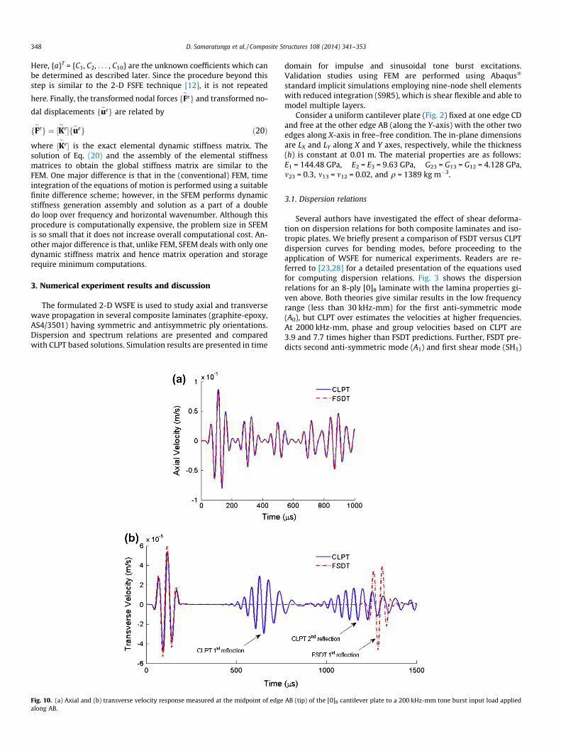
Fig. 10. (a) Axial and (b) transverse velocity response measured at the midpoint of edgealong AB.

domain for impulse and sinusoidal tone burst excitations.Validation studies using FEM are performed using Abaqus�

standard implicit simulations employing nine-node shell elementswith reduced integration (S9R5), which is shear flexible and able tomodel multiple layers.

Consider a uniform cantilever plate (Fig. 2) fixed at one edge CDand free at the other edge AB (along the Y-axis) with the other twoedges along X-axis in free–free condition. The in-plane dimensionsare LX and LY along X and Y axes, respectively, while the thickness(h) is constant at 0.01 m. The material properties are as follows:E1 = 144.48 GPa, E2 = E3 = 9.63 GPa, G23 = G13 = G12 = 4.128 GPa,m23 = 0.3, m13 = m12 = 0.02, and q = 1389 kg m�3.

3.1. Dispersion relations

Several authors have investigated the effect of shear deforma-tion on dispersion relations for both composite laminates and iso-tropic plates. We briefly present a comparison of FSDT versus CLPTdispersion curves for bending modes, before proceeding to theapplication of WSFE for numerical experiments. Readers are re-ferred to [23,28] for a detailed presentation of the equations usedfor computing dispersion relations. Fig. 3 shows the dispersionrelations for an 8-ply [0]8 laminate with the lamina properties gi-ven above. Both theories give similar results in the low frequencyrange (less than 30 kHz-mm) for the first anti-symmetric mode(A0), but CLPT over estimates the velocities at higher frequencies.At 2000 kHz-mm, phase and group velocities based on CLPT are3.9 and 7.7 times higher than FSDT predictions. Further, FSDT pre-dicts second anti-symmetric mode (A1) and first shear mode (SH1)

AB (tip) of the [0]8 cantilever plate to a 200 kHz-mm tone burst input load applied

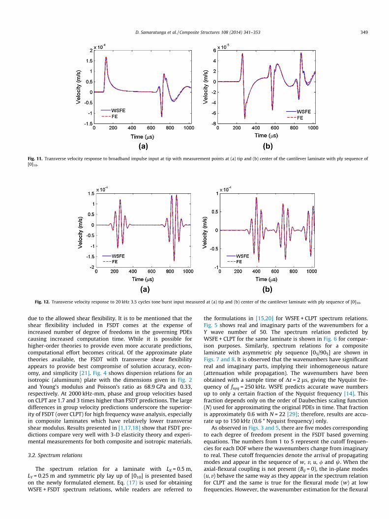
Fig. 11. Transverse velocity response to broadband impulse input at tip with measurement points at (a) tip and (b) center of the cantilever laminate with ply sequence of[0]10.

Fig. 12. Transverse velocity response to 20 kHz 3.5 cycles tone burst input measured at (a) tip and (b) center of the cantilever laminate with ply sequence of [0]10.

D. Samaratunga et al. / Composite Structures 108 (2014) 341–353 349

due to the allowed shear flexibility. It is to be mentioned that theshear flexibility included in FSDT comes at the expense ofincreased number of degree of freedoms in the governing PDEscausing increased computation time. While it is possible forhigher-order theories to provide even more accurate predictions,computational effort becomes critical. Of the approximate platetheories available, the FSDT with transverse shear flexibilityappears to provide best compromise of solution accuracy, econ-omy, and simplicity [21]. Fig. 4 shows dispersion relations for anisotropic (aluminum) plate with the dimensions given in Fig. 2and Young’s modulus and Poisson’s ratio as 68.9 GPa and 0.33,respectively. At 2000 kHz-mm, phase and group velocities basedon CLPT are 1.7 and 3 times higher than FSDT predictions. The largedifferences in group velocity predictions underscore the superior-ity of FSDT (over CLPT) for high frequency wave analysis, especiallyin composite laminates which have relatively lower transverseshear modulus. Results presented in [1,17,18] show that FSDT pre-dictions compare very well with 3-D elasticity theory and experi-mental measurements for both composite and isotropic materials.

3.2. Spectrum relations

The spectrum relation for a laminate with LX = 0.5 m,LY = 0.25 m and symmetric ply lay up of [010] is presented basedon the newly formulated element. Eq. (17) is used for obtainingWSFE + FSDT spectrum relations, while readers are referred to

the formulations in [15,20] for WSFE + CLPT spectrum relations.Fig. 5 shows real and imaginary parts of the wavenumbers for aY wave number of 50. The spectrum relation predicted byWSFE + CLPT for the same laminate is shown in Fig. 6 for compar-ison purposes. Similarly, spectrum relations for a compositelaminate with asymmetric ply sequence [05/905] are shown inFigs. 7 and 8. It is observed that the wavenumbers have significantreal and imaginary parts, implying their inhomogeneous nature(attenuation while propagation). The wavenumbers have beenobtained with a sample time of Dt = 2 ls, giving the Nyquist fre-quency of fnyq = 250 kHz. WSFE predicts accurate wave numbersup to only a certain fraction of the Nyquist frequency [14]. Thisfraction depends only on the order of Daubechies scaling function(N) used for approximating the original PDEs in time. That fractionis approximately 0.6 with N = 22 [29]; therefore, results are accu-rate up to 150 kHz (0.6 * Nyquist frequency) only.

As observed in Figs. 3 and 5, there are five modes correspondingto each degree of freedom present in the FSDT based governingequations. The numbers from 1 to 5 represent the cutoff frequen-cies for each DOF where the wavenumbers change from imaginaryto real. These cutoff frequencies denote the arrival of propagatingmodes and appear in the sequence of w, v, u, / and w. When theaxial-flexural coupling is not present (Bij = 0), the in-plane modes(u,v) behave the same way as they appear in the spectrum relationfor CLPT and the same is true for the flexural mode (w) at lowfrequencies. However, the wavenumber estimation for the flexural

350 D. Samaratunga et al. / Composite Structures 108 (2014) 341–353

mode is under predicted by CLPT at high frequencies in the absenceof rotary inertia and transverse shear flexibility terms in the for-mulation. First shear mode (/) becomes real after the fourth cutofffrequency whereas the corresponding mode for CLPT (dw/dx) iscompletely imaginary at high frequencies. The second shear mode(w) is an additional mode appearing in FSDT results only, whichstarts propagating after the fifth cutoff frequency.

Moreover, the imaginary parts of the shear wave numbers havehigher magnitudes compared to the imaginary parts of the fourthwave number in CLPT. This indicates comparatively higher modaldamping obtained in the FSDT simulations. As happened in CLPT,both w and / wave numbers initially contain nonzero real andimaginary parts denoting the propagation of inhomogeneouswaves. When considering the laminate with asymmetric ply

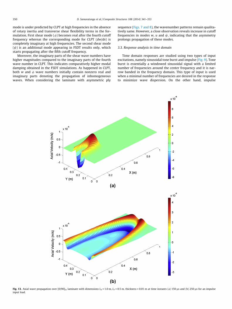
Fig. 13. Axial wave propagation over [0/90]2s laminate with dimensions LX = 1.0 m, LY =input load.

sequence (Figs. 7 and 8), the wavenumber patterns remain qualita-tively same. However, a close observation reveals increase in cutofffrequencies in modes w, u and w, indicating that the asymmetryprolongs propagation of these modes.

3.3. Response analysis in time domain

Time domain responses are studied using two types of inputexcitations, namely sinusoidal tone burst and impulse (Fig. 9). Toneburst is essentially a windowed sinusoidal signal with a limitednumber of frequencies around the center frequency and it is nar-row banded in the frequency domain. This type of input is usedwhen a minimal number of frequencies are desired in the responseto minimize wave dispersion. On the other hand, impulse

0.5 m, thickness = 0.01 m at time instants (a) 150 ls and (b) 250 ls for an impulse

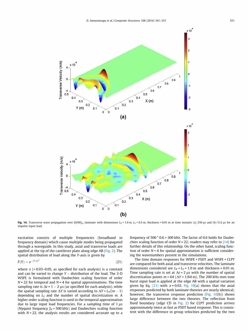
Fig. 14. Transverse wave propagation over [0/90]2s laminate with dimensions LX = 1.0 m, LY = 0.5 m, thickness = 0.01 m at time instants (a) 250 ls and (b) 512 ls for animpulse input load.

D. Samaratunga et al. / Composite Structures 108 (2014) 341–353 351

excitation consists of multiple frequencies (broadband infrequency domain) which cause multiple modes being propagatedthrough a waveguide. In this study, axial and transverse loads areapplied at the tip of the cantilever plate along edge AB (Fig. 2). Thespatial distribution of load along the Y-axis is given by

FðYÞ ¼ e�ðY=aÞ2 ð21Þ

where a (= 0.03–0.05, as specified for each analysis) is a constantand can be varied to change Y – distribution of the load. The 2-DWSFE is formulated with Daubechies scaling function of orderN = 22 for temporal and N = 4 for spatial approximations. The timesampling rate is Dt = 1 � 2 ls (as specified for each analysis), whilethe spatial sampling rate DY is varied according to DY = LY/(m � 1)depending on LY and the number of spatial discretization m. Ahigher order scaling function is used in the temporal approximationdue to large input load frequencies. For a sampling time of 1 ls(Nyquist frequency fN = 500 kHz) and Daubechies scaling functionwith N = 22, the analysis results are considered accurate up to a

frequency of 500 * 0.6 = 300 kHz. The factor of 0.6 holds for Daube-chies scaling function of order N = 22; readers may refer to [14] forfurther details of this relationship. On the other hand, scaling func-tion of order N = 4 for spatial approximation is sufficient consider-ing the wavenumbers present in the simulations.

The time domain responses for WSFE + FSDT and WSFE + CLPTare compared for both axial and transverse velocities. The laminatedimensions considered are LX = LY = 1.0 m and thickness = 0.01 m.Time sampling rate is set at Dt = 2 ls with the number of spatialdiscretization points m = 64 (DY = 1/64 m). The 200 kHz-mm toneburst input load is applied at the edge AB with a spatial variationgiven by Eq. (21) with a = 0.03. Fig. 10(a) shows that the axialresponses predicted by both laminate theories are nearly identical;however, the transverse response prediction (Fig. 10(b)) showslarge difference between the two theories. The reflection fromfixed boundary (edge CD in Fig. 2) for CLPT prediction arrivesapproximately twice as fast as FSDT based response. This is consis-tent with the difference in group velocities predicted by the two

352 D. Samaratunga et al. / Composite Structures 108 (2014) 341–353

theories as shown in Fig. 3(b). Another significant difference is thatthe group velocity based on FSDT is non-dispersive at this fre-quency-thickness, whereas CLPT prediction is in the dispersive re-gion. Therefore, the fixed boundary reflection using FSDT retainsthe shape of the excited wave packet, but CLPT shows a highly dis-persed wave. In summary, transverse shear and rotary inertia havehighly significant effect on the wave motion at high frequencieswhich necessitates the use of FSDT for accurate predictions.

3.4. Validation with conventional FEM

WSFE + FSDT results are compared with finite element simula-tions using Abaqus� standard implicit direct solver [25]. The lam-inate has dimensions of LX = LY = 0.5 m, time sampling rateDt = 1 ls with the number of spatial discretization points m = 64(DY = 1/64 m). Both unit impulse and tone burst input loads areapplied at the edge AB with a spatial variation given by Eq. (21)with a = 0.05. In the absence of any discontinuity, it is sufficientto model the uniform laminate structure shown in Fig. 2 using justone element in WSFE. Abaqus� model required a very refined meshwith 7688 nine-node shell elements (S9R5) for high frequency sim-ulations. As a result, WSFE analysis takes only 44s, whereas Aba-qus� simulation takes 4379s, which is two orders of magnitudehigher than WSFE. Figs. 11 and 12 show transverse velocities mea-sured at two points on the laminate (mid-point of tip and center ofthe laminate) for impulse and tone burst inputs, respectively. It isobserved that WSFE + FSDT and Abaqus� results have excellentcorrelation.

The first peak of tip response shown in Fig. 11(a) is the incidentimpulse which lasts for only a short time. For an impulse (broadband) input, each frequency component propagates at its groupvelocity and the fixed boundary reflection has multiple wave com-ponents with the fastest one reaching the tip at approximately700 ls. Responses measured at the center of the laminate(Fig. 11(b)) show several reflections, including the first one arrivingsoon after the incident impulse. For a sinusoidal tone burst input(Fig. 12), both forward propagating and reflected wave packetsare concentrated in time as well as frequency domains. As notedearlier, the wave motion is non-dispersive at this frequency-thick-ness (200 kHz-mm) thus preserving the shape of the wave packet.Most of the Lamb wave based SHM techniques employ sinusoidaltone burst input which makes signal interpretation less difficultin the non-dispersive frequency range [7].

3.5. Axial and transverse wave visualization

The wavenumbers and amplitude ratios (j and d0)obtained bysolving Eq. (17), are used along with the relation between trans-formed nodal forces and displacements (Eq. (20)) to determinethe unknown coefficients {a} in Eq. (19). Then Eq. (19) gives thedisplacement at any X 2 [0,LX] in the transformed frequency-wave-number domain. The wave velocities at sampling points alongY-axis and at any point along X-axis can then be obtained from asingle simulation. For wave visualization, the laminate dimensionsconsidered are LX = 1.0 m, LY = 0.5 m and thickness = 0.01 m with asymmetric ply layup of [0/90]2s. Time sampling rate is set atDt = 2 ls with the number of spatial discretization points m = 64(DY = 1/64 m). Fig. 13 shows the axial wave propagation in thelaminate at two different time instants for an unit impulse inputload applied at edge AB (Fig. 2) with a spatial variation given byEq. (21) with a = 0.03. Since the axial waves travel non-dispersively, time domain response preserves the shape of the ex-cited wave packet for any propagated distance. Further, Fig. 13(b)shows the directional dependence of the wave velocity. For thecross-ply laminate configuration, the stiffness is highest in 0� and90� directions, resulting in the highest wave velocity along them.

Fig. 14 shows the flexural wave response of the plate for an im-pulse input load applied in the transverse direction. It is observedthat the flexural (anti-symmetric) wave propagation velocity ismuch smaller than the axial (symmetric) wave propagation veloc-ity (Fig. 13) for this input load bandwidth. Further, Fig. 14(b) showsthe dispersive nature of the anti-symmetric mode. The wave is dis-persed all over the plate due to multiple wave components withdifferent group velocities.

4. Concluding remarks

A new 2-D wavelet spectral finite element (WSFE) with sheardeformation was presented for accurate modeling of high fre-quency wave propagation in anisotropic composite laminates.The governing PDEs based on FSDT were used to account for trans-verse shear strains and rotary inertia. Daubechies compactly sup-ported, orthonormal, scaling functions were employed fortemporal and spatial approximations to reduce the governing PDEsto ODEs in one spatial variable only. An eigenvalue analysis wasused to decouple ODEs which were solved exactly to obtain theshape functions used in the element formulation. Since the devel-oped element captured the exact inertial distribution, a single ele-ment was sufficient to model a laminate of any dimension in theabsence of discontinuities. Further, due to the compact nature ofDaubechies scaling functions, the WSFE was able to model finitewaveguides without the signal ‘wraparound’ problem (associatedwith Fourier transform based spectral finite element).

Group/phase velocity dispersion relations for fundamental anti-symmetric mode were compared between FSDT and CLPT showinglarge discrepancy at high frequencies, especially in the case ofcomposite laminates which have lower transverse shear modulus(compared to isotropic materials such as aluminum). Spectrumrelations describing the relationship between wavenumber andfrequency were presented and compared for the two theories(FSDT and CLPT). The wavenumbers showed both real and imagi-nary parts indicating attenuation while propagating. Comparisonbetween different ply sequences showed that the asymmetric plysequence ([05/905]) prolonged the cutoff frequency, the critical fre-quency where the wavenumber changed from imaginary to real.Time domain analysis was performed for two types of input loads,narrowband tone burst and broadband impulse. Axial wave prop-agation showed similarity between FSDT and CLPT, but flexuralwave velocity was much faster for CLPT resulting in spuriousboundary reflections. The developed WSFE was validated withAbaqus� FEM simulations using shear flexible elements. Excellentcorrelation was observed in the results and WSFE computationtime was less than two orders of magnitude compared to Abaqus�.Finally, a few snapshots at different time instants were presentedto visualize the wave motion in composite laminates using WSFEsimulations.

Acknowledgments

The authors gratefully acknowledge partial funding for this re-search through AFOSR Grant Number FA9550-09-1-0275 (ProgramManagers: Dr. Victor Giurgiutiu and Dr. David Stargel).

References

[1] Graff KF. Wave motion in elastic solids. Mineola (NY): Dover Publications Inc.,;1991 [11501].

[2] Rose JL. Ultrasonic waves in solid media. New York: Cambridge UniversityPress; 2004.

[3] Nayfeh AH. Wave propagation in layered anisotropic media: with applicationsto composites, vol. 39. North Holland; 1995.

[4] Datta SK, Shah AH. Elastic waves in composite media and structures: withapplications to ultrasonic nondestructive evaluation. CRC Press; 2008.

D. Samaratunga et al. / Composite Structures 108 (2014) 341–353 353

[5] Chimenti DE. Guided waves in plates and their use in materialscharacterization. Appl Mech Rev 1997;50:247–84.

[6] Raghavan A, Cesnik C. Review of guided-wave structural health monitoring.Shock Vib Dig 2007;39:91–114.

[7] Giurgiutiu V. Structural health monitoring: with piezoelectric wafer activesensors. MA: Elsevier; 2008.

[8] Su Z, Ye L, Lu Y. Guided lamb waves for identification of damage in compositestructures: a review. J Sound Vib 2006;295:753–80.

[9] Boller C, Chang F-K, Fujino Y. Encyclopedia of structural healthmonitoring. West Sussex (UK): John Wiley & Sons Ltd.; 2009.

[10] Diamanti K, Soutis C. Structural health monitoring techniques for aircraftcomposite structures. Prog Aerosp Sci 2010;46:342–52.

[11] Ochoa OO, Reddy JN. Finite element analysis of composite laminates, vol.7. Springer; 1992.

[12] Doyle JF. Wave propagation in structures: spectral analysis using fast discreteFourier transforms. 2nd ed. New York: Springer-Verlag; 1997.

[13] Gopalakrishnan S, Roy Mahapatra D, Chakraborty A. Spectral finite elementmethod. London (United Kingdom): Springer-Verlag; 2007.

[14] Gopalakrishnan S, Mitra M. Wavelet methods for dynamical problems. BocaRaton (FL): CRC Press; 2010.

[15] Chakraborty A, Gopalakrishnan S. A spectrally formulated plate element forwave propagation analysis in anisotropic material. Comput Methods ApplMech Eng 2005;194:4425–46.

[16] Daubechies I. Ten lectures on wavelets, vol. 61. Philadelphia: Society forIndustrial and Applied Mathematics; 1992.

[17] Mitra M, Gopalakrishnan S. Spectrally formulated wavelet finite element forwave propagation and impact force identification in connected 1-Dwaveguides. Int J Solids Struct 2005;42:4695–721.

[18] Mitra M, Gopalakrishnan S. Wavelet based spectral finite element for analysisof coupled wave propagation in higher order composite beams. Compos Struct2006;73:263–77.

[19] Mitra M, Gopalakrishnan S. Wavelet based 2-D spectral finite elementformulation for wave propagation analysis in isotropic plates. Comput ModelEng Sci 2006;1:11–29.

[20] Mitra M, Gopalakrishnan S. Wave propagation analysis in anisotropic plateusing wavelet spectral element approach. J Appl Mech 2008;75:014504-1–4-6.

[21] Reddy JN. Mechanics of laminated composite plates and shells. Boca Raton:CRC Press; 2004.

[22] Prosser WH, Gorman MR. Plate mode velocities in graphite/epoxy plates. JAcoust Soc Am 1994;96:902–7.

[23] Tang B, Henneke II EG, Stiffler RC. Low frequency flexural wave propagation inlaminated composite plates. Plenum Press; 1988.

[24] Rose LRF, Wang CH. Mindlin plate theory for damage detection: sourcesolutions. J Acoust Soc Am 2004;116:154–71.

[25] Abaqus Theory Manual. Version 6.12-1. Providence (RI): Dassault SystémesSimulia Corp.

[26] Beylkin G. On the representation of operators in bases of compactly supportedwavelets. SIAM J Numer Anal 1992;6:1716–40.

[27] Williams JR, Amaratunga K. A discrete wavelet transform without edge effectsusing wavelet extrapolation. J Fourier Anal Appl 1997;3:435–49.

[28] Duke Jr JC, Henneke II EG, Stinchcomb WW, Ultrason. Stress wave charact ofcomposite mater. NASA contractor report 3976; 1986.

[29] Mitra M, Gopalakrishnan S. Extraction of wave characteristics from waveletbased spectral finite element formulation. Mech Syst Signal Process 2006;20:2046–79.