4 State-space solutions and realizations

• 4.2 Solutions of LTI State EquationsConsider

• Premultiplying on both sides of first yields

• Implies

⎩⎨⎧

+=+=

)t(Du)t(Cx)t(y)t(Bu)t(Ax)t(x&

Ate−

)t(Bue)t(Axe)t(xe AtAtAt −−− =−&)t(Bue))t(xe(

dtd AtAt −− =

• Its integration from 0 to t yields

• Thus, we have

• The final solution

• Compute the solutions by using Laplacetransform

τ∫ τ=τ τ−=τ

− d)(Bue)(xe t0

At0

At

τ∫ τ+= τ− d)(Bue)0(xe)t(x t0

)t(AAt

)t(Dud)(BueC)0(xCe)t(y t0

)t(AAt +τ∫ τ+= τ−

)]s(uB)0(x[)AsI()s(x 1 +−= −

)s(uD)]s(uB)0(x[)AsI(C)s(y 1 ++−= −

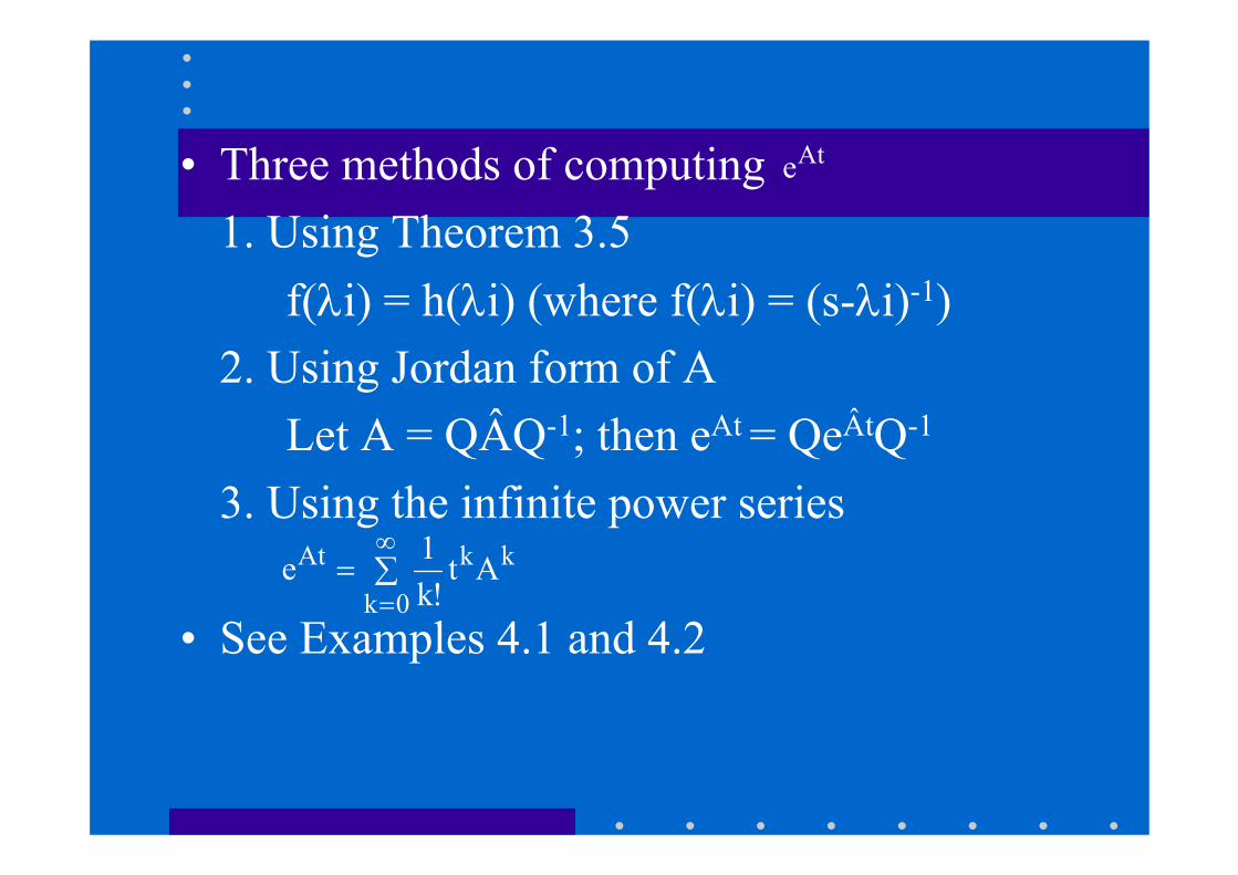
• Three methods of computing1. Using Theorem 3.5

f(λi) = h(λi) (where f(λi) = (s-λi)-1)2. Using Jordan form of A

Let A = QÂQ-1; then eAt = QeÂtQ-1

3. Using the infinite power series

• See Examples 4.1 and 4.2

Ate

∑=∞

=0k

kkAt At!k

1e

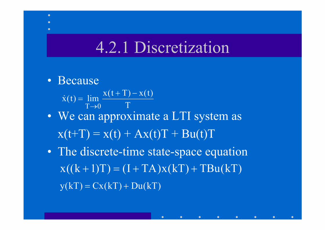
4.2.1 Discretization

• Because

• We can approximate a LTI system asx(t+T) = x(t) + Ax(t)T + Bu(t)T

• The discrete-time state-space equation

T)t(x)Tt(xlim)t(x

0T

−+=

→&

)kT(TBu)kT(x)TAI()T)1k((x ++=+)kT(Du)kT(Cx)kT(y +=

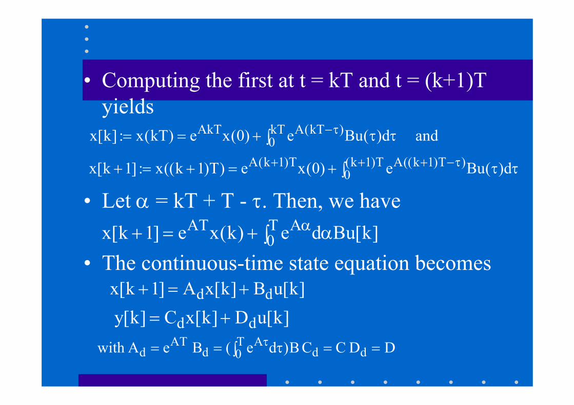
• Computing the first at t = kT and t = (k+1)T yields

• Let α = kT + T - τ. Then, we have

• The continuous-time state equation becomes

∫ ττ+== τ−kT0

)kT(AAkT and d)(Bue)0(xe)kT(x:]k[x

∫ ττ+=+=+ + τ−++ T)1k(0

)T)1k((AT)1k(A d)(Bue)0(xe)T)1k((x:]1k[x

∫ α+=+ αT0

AAT ]k[Bude)k(xe]1k[x

]k[uB]k[xA]1k[x dd +=+

]k[uD]k[xC]k[y dd +=

D DCC B)de( BeA with ddT0

Ad

ATd ==∫ τ== τ

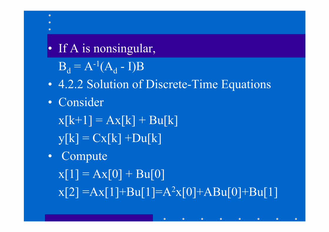
• If A is nonsingular,Bd = A-1(Ad - I)B

• 4.2.2 Solution of Discrete-Time Equations• Consider

x[k+1] = Ax[k] + Bu[k]y[k] = Cx[k] +Du[k]

• Computex[1] = Ax[0] + Bu[0]x[2] =Ax[1]+Bu[1]=A2x[0]+ABu[0]+Bu[1]

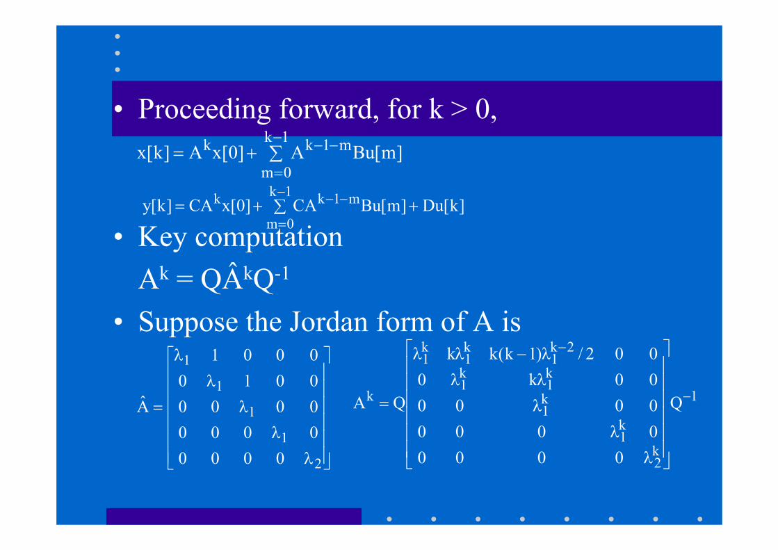
• Proceeding forward, for k > 0,

• Key computationAk = QÂkQ-1

• Suppose the Jordan form of A is

∑+=−

=

−−1k

0m

m1kk ]m[BuA]0[xA]k[x

∑ ++=−

=

−−1k

0m

m1kk ]k[Du]m[BuCA]0[xCA]k[y

⎥⎥⎥⎥⎥⎥

⎦

⎤

⎢⎢⎢⎢⎢⎢

⎣

⎡

λλ

λλ

λ

=

2

1

1

1

1

00000000000000100001

A1

k2

k1

k1

k1

k1

2k1

k1

k1

k Q

00000000000000k0002/)1k(kk

QA −

−

⎥⎥⎥⎥⎥⎥

⎦

⎤

⎢⎢⎢⎢⎢⎢

⎣

⎡

λλ

λλλλ−λλ

=

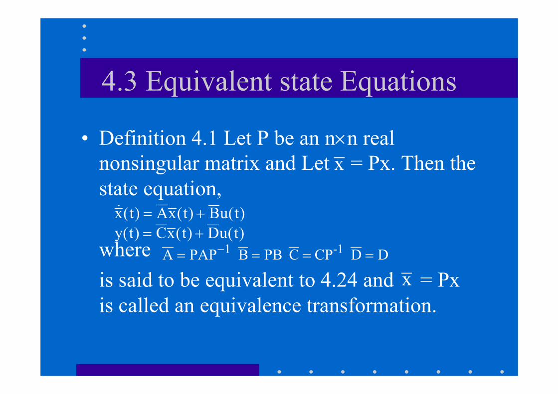
4.3 Equivalent state Equations

• Definition 4.1 Let P be an n×n real nonsingular matrix and Let = Px. Then the state equation,

where is said to be equivalent to 4.24 and = Pxis called an equivalence transformation.

x

)t(uB)t(xA)t(x +=&

)t(uD)t(xC)t(y +=DD CPC PBB PAPA -11 ==== −

x

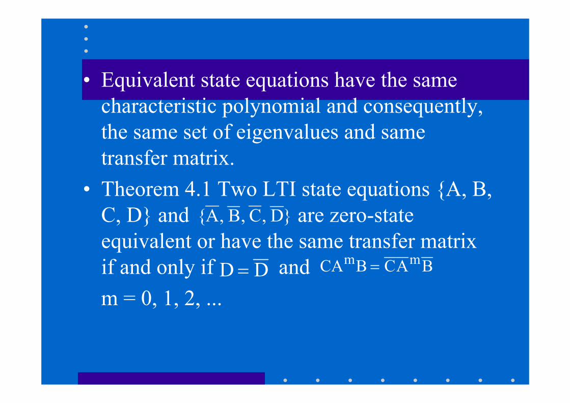
• Equivalent state equations have the same characteristic polynomial and consequently, the same set of eigenvalues and same transfer matrix.

• Theorem 4.1 Two LTI state equations {A, B, C, D} and are zero-state equivalent or have the same transfer matrix if and only if and m = 0, 1, 2, ...

}D ,C ,B ,A{

DD = BACBCA mm =

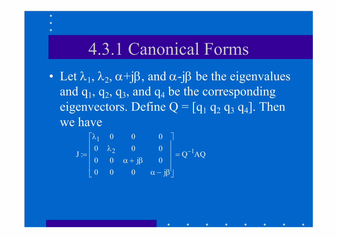
4.3.1 Canonical Forms• Let λ1, λ2, α+jβ, and α-jβ be the eigenvalues

and q1, q2, q3, and q4 be the corresponding eigenvectors. Define Q = [q1 q2 q3 q4]. Then we have

AQQ

j0000j00000000

:J 12

1

−=

⎥⎥⎥⎥

⎦

⎤

⎢⎢⎢⎢

⎣

⎡

β−αβ+α

λλ

=

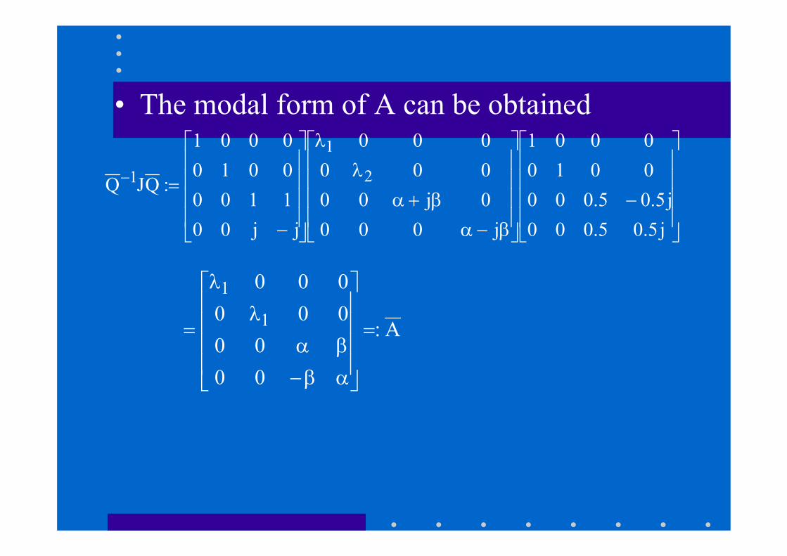
• The modal form of A can be obtained

A:

0000

000000

1

1

=

⎥⎥⎥⎥

⎦

⎤

⎢⎢⎢⎢

⎣

⎡

αβ−βα

λλ

=

⎥⎥⎥⎥

⎦

⎤

⎢⎢⎢⎢

⎣

⎡

−⎥⎥⎥⎥

⎦

⎤

⎢⎢⎢⎢

⎣

⎡

β−αβ+α

λλ

⎥⎥⎥⎥

⎦

⎤

⎢⎢⎢⎢

⎣

⎡

−

=−

j5.05.000j5.05.000

00100001

j0000j00000000

jj00110000100001

:QJQ 2

1

1

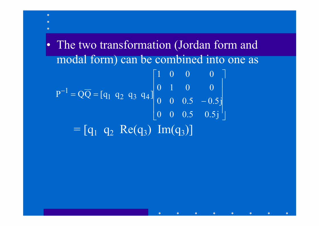
• The two transformation (Jordan form and modal form) can be combined into one as

= [q1 q2 Re(q3) Im(q3)]

⎥⎥⎥⎥

⎦

⎤

⎢⎢⎢⎢

⎣

⎡

−==−

j5.05.000j5.05.000

00100001

]q q q q[QQP 43211

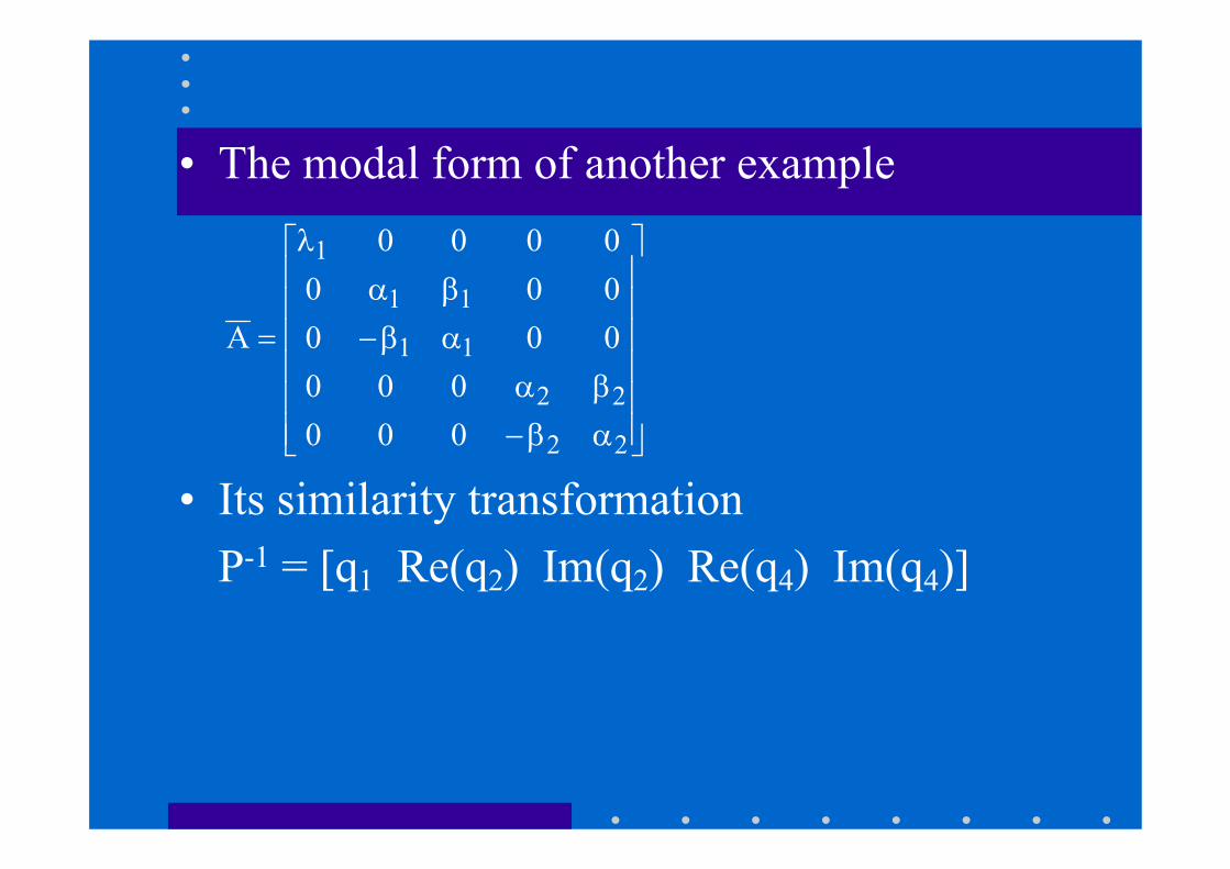
• The modal form of another example

• Its similarity transformationP-1 = [q1 Re(q2) Im(q2) Re(q4) Im(q4)]

⎥⎥⎥⎥⎥⎥

⎦

⎤

⎢⎢⎢⎢⎢⎢

⎣

⎡

αβ−βα

αβ−βα

λ

=

22

22

11

11

1

000000

0000000000

A

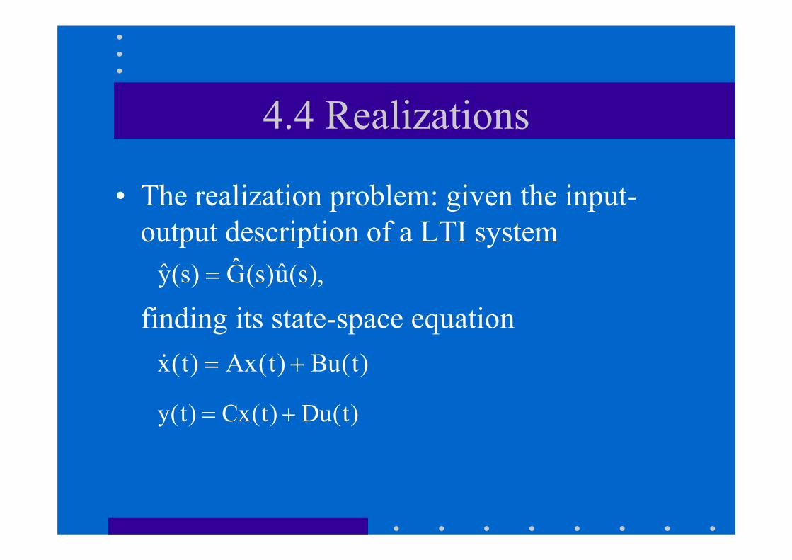
4.4 Realizations

• The realization problem: given the input-output description of a LTI system

finding its state-space equation),s(u)s(G)s(y =

)t(Bu)t(Ax)t(x +=&

)t(Du)t(Cx)t(y +=

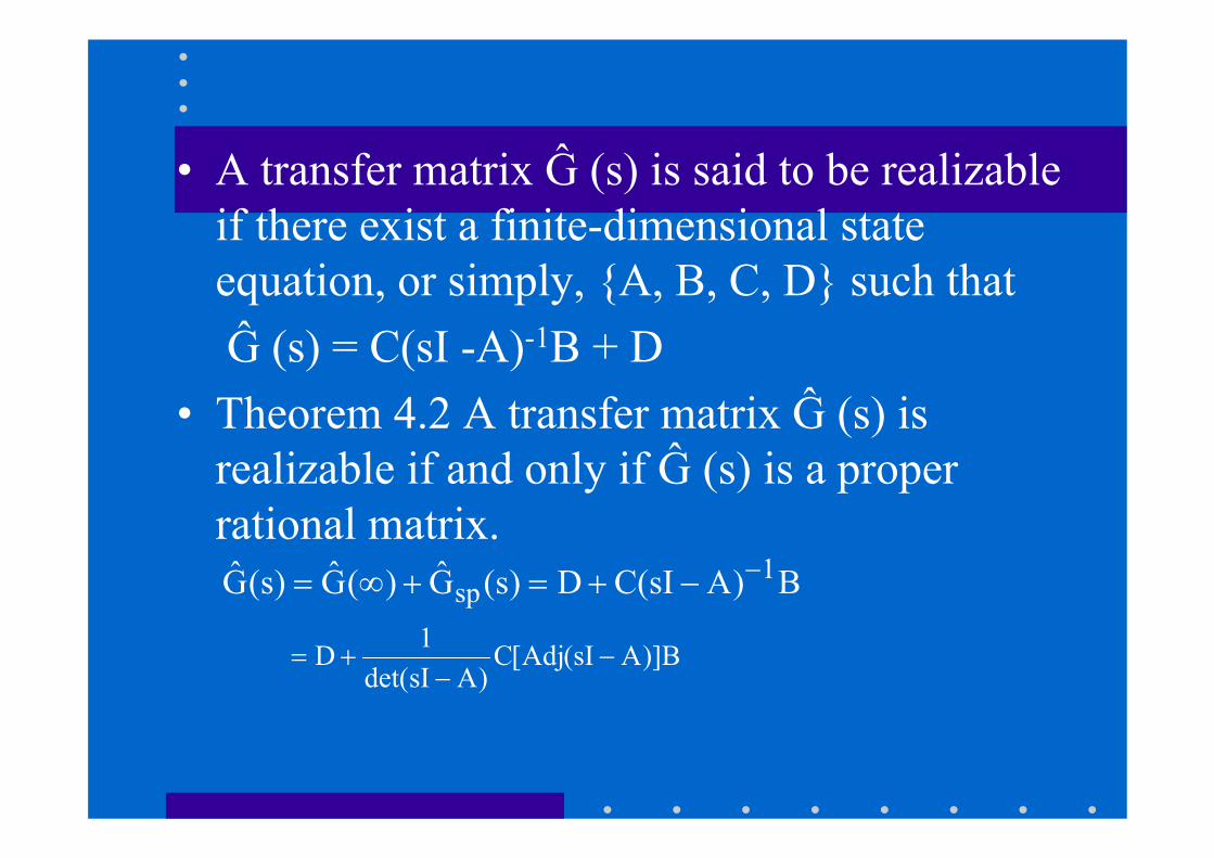
• A transfer matrix Ĝ (s) is said to be realizable if there exist a finite-dimensional state equation, or simply, {A, B, C, D} such that Ĝ (s) = C(sI -A)-1B + D

• Theorem 4.2 A transfer matrix Ĝ (s) is realizable if and only if Ĝ (s) is a proper rational matrix.

B)AsI(CD)s(G)(G)s(G 1sp

−−+=+∞=

B)]AsI(Adj[C)AsIdet(

1D −−

+=

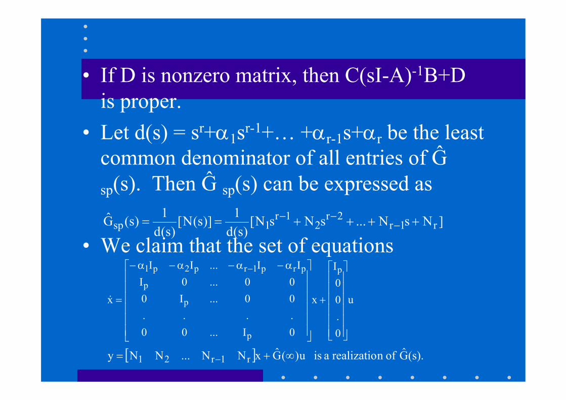
• If D is nonzero matrix, then C(sI-A)-1B+D is proper.

• Let d(s) = sr+α1sr-1+… +αr-1s+αr be the least common denominator of all entries of Ĝsp(s). Then Ĝ sp(s) can be expressed as

• We claim that the set of equations]NsN...sNsN[

)s(d1)]s(N[

)s(d1)s(G r1r

2r2

1r1sp ++++== −

−−

u

0.00I

x

0I...00....00...I000...0I

II...II

x

p

p

p

p

prp1rp2p1

⎥⎥⎥⎥⎥⎥

⎦

⎤

⎢⎢⎢⎢⎢⎢

⎣

⎡

+

⎥⎥⎥⎥⎥⎥

⎦

⎤

⎢⎢⎢⎢⎢⎢

⎣

⎡ α−α−α−α−

=

−

&

[ ] (s).G of nrealizatioa is u)(GxNN...NNy r1r21 ∞+= −

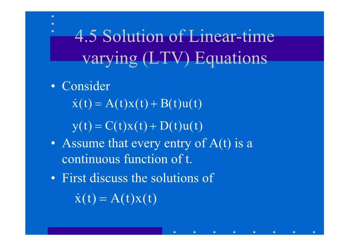
4.5 Solution of Linear-time varying (LTV) Equations

• Consider

• Assume that every entry of A(t) is a continuous function of t.

• First discuss the solutions of

)t(u)t(B)t(x)t(A)t(x +=&

)t(u)t(D)t(x)t(C)t(y +=

)t(x)t(A)t(x =&

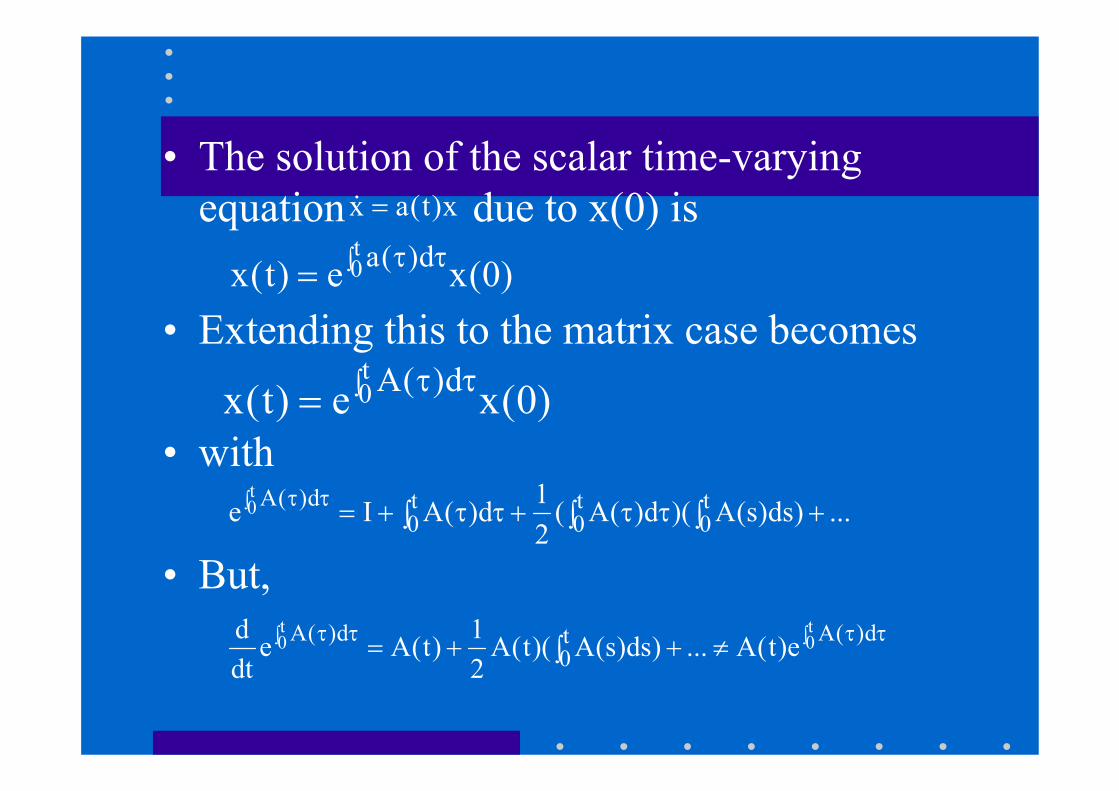
• The solution of the scalar time-varying equation due to x(0) is

• Extending this to the matrix case becomes

• with

• But,

x)t(ax =&

)0(xe)t(xt0 d)(a∫ ττ=

)0(xe)t(xt0 d)(A∫ ττ=

...)ds)s(A)(d)(A(21d)(AIe t

0t0

t0

d)(At0 +∫∫ ττ+∫ ττ+=∫ ττ

∫∫ ττττ ≠+∫+=t0

t0 d)(At

0d)(A e)t(A...)ds)s(A)(t(A

21)t(Ae

dtd

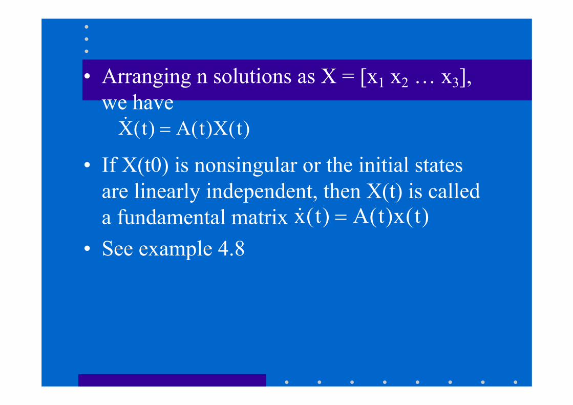
• Arranging n solutions as X = [x1 x2 … x3], we have

• If X(t0) is nonsingular or the initial states are linearly independent, then X(t) is called a fundamental matrix

• See example 4.8

)t(X)t(A)t(X =&

)t(x)t(A)t(x =&

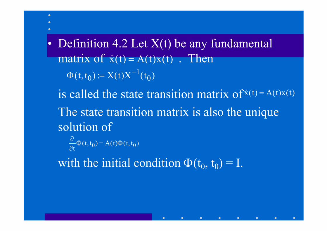
• Definition 4.2 Let X(t) be any fundamental matrix of . Then

is called the state transition matrix ofThe state transition matrix is also the unique solution of

with the initial condition Φ(t0, t0) = I.

)t(x)t(A)t(x =&

)t(X)t(X:)t,t( 01

0−=Φ

)t(x)t(A)t(x =&

)t,t()t(A)t,t(t 00 Φ=Φ∂∂

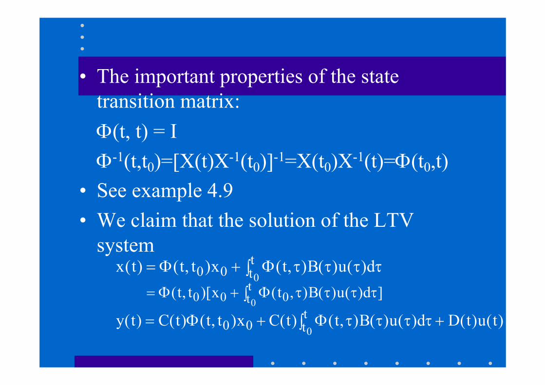
• The important properties of the state transition matrix:Φ(t, t) = IΦ-1(t,t0)=[X(t)X-1(t0)]-1=X(t0)X-1(t)=Φ(t0,t)

• See example 4.9• We claim that the solution of the LTV

system∫ ττττΦ+Φ= tt00 0

d)(u)(B),t(x)t,t()t(x]d)(u)(B),t(x)[t,t( t

t 000 0∫ ττττΦ+Φ=

)t(u)t(Dd)(u)(B),t()t(Cx)t,t()t(C)t(y tt00 0

+∫ ττττΦ+Φ=

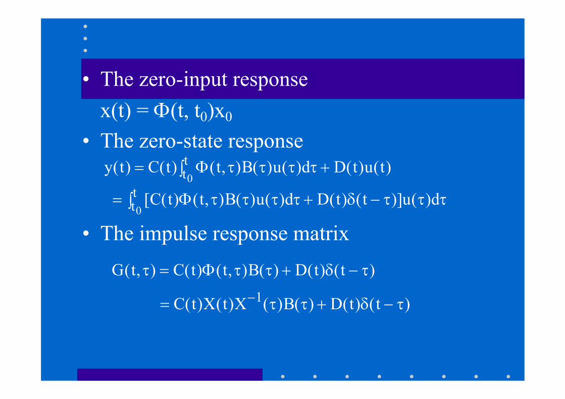
• The zero-input responsex(t) = Φ(t, t0)x0

• The zero-state response

• The impulse response matrix

)t(u)t(Dd)(u)(B),t()t(C)t(y tt0

+∫ ττττΦ=

τττ−δ+∫ ττττΦ= d)(u)]t()t(Dd)(u)(B),t()t(C[tt0

)t()t(D)(B),t()t(C),t(G τ−δ+ττΦ=τ

)t()t(D)(B)(X)t(X)t(C 1 τ−δ+ττ= −

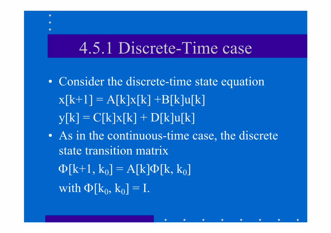
4.5.1 Discrete-Time case

• Consider the discrete-time state equationx[k+1] = A[k]x[k] +B[k]u[k]y[k] = C[k]x[k] + D[k]u[k]

• As in the continuous-time case, the discrete state transition matrixΦ[k+1, k0] = A[k]Φ[k, k0]with Φ[k0, k0] = I.

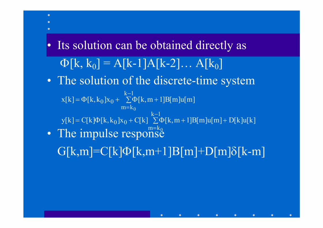
• Its solution can be obtained directly asΦ[k, k0] = A[k-1]A[k-2]… A[k0]

• The solution of the discrete-time system

• The impulse responseG[k,m]=C[k]Φ[k,m+1]B[m]+D[m]δ[k-m]

∑ +Φ+Φ=−

=

1k

km00

0

]m[u]m[B]1m,k[x]k,k[]k[x

]k[u]k[D]m[u]m[B]1m,k[]k[Cx]k,k[]k[C]k[y1k

km00

0

+∑ +Φ+Φ=−

=

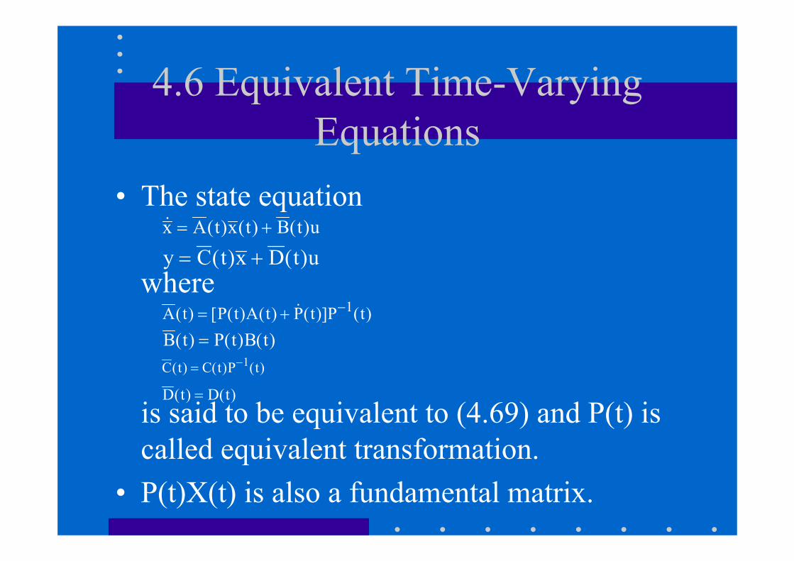
4.6 Equivalent Time-Varying Equations

• The state equation

where

is said to be equivalent to (4.69) and P(t) is called equivalent transformation.

• P(t)X(t) is also a fundamental matrix.

u)t(B)t(x)t(Ax +=&

u)t(Dx)t(Cy +=

)t(P)]t(P)t(A)t(P[)t(A 1−+= &

)t(B)t(P)t(B =)t(P)t(C)t(C 1−=

)t(D)t(D =

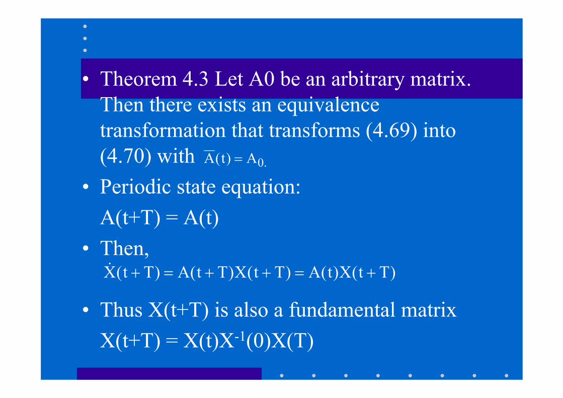
• Theorem 4.3 Let A0 be an arbitrary matrix. Then there exists an equivalence transformation that transforms (4.69) into (4.70) with

• Periodic state equation:A(t+T) = A(t)

• Then,

• Thus X(t+T) is also a fundamental matrixX(t+T) = X(t)X-1(0)X(T)

.0A)t(A =

)Tt(X)t(A)Tt(X)Tt(A)Tt(X +=++=+&

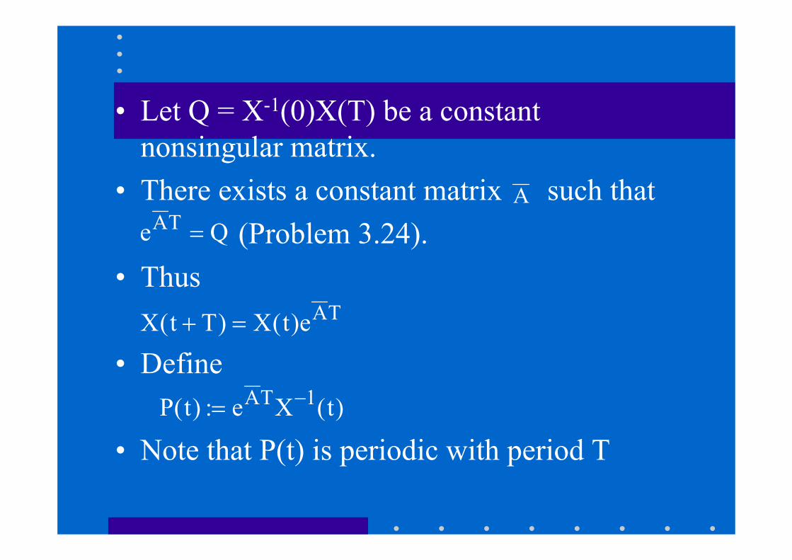
• Let Q = X-1(0)X(T) be a constant nonsingular matrix.

• There exists a constant matrix such that (Problem 3.24).

• Thus

• Define

• Note that P(t) is periodic with period T

A

Qe TA =

TAe)t(X)Tt(X =+

)t(Xe:)t(P 1TA −=

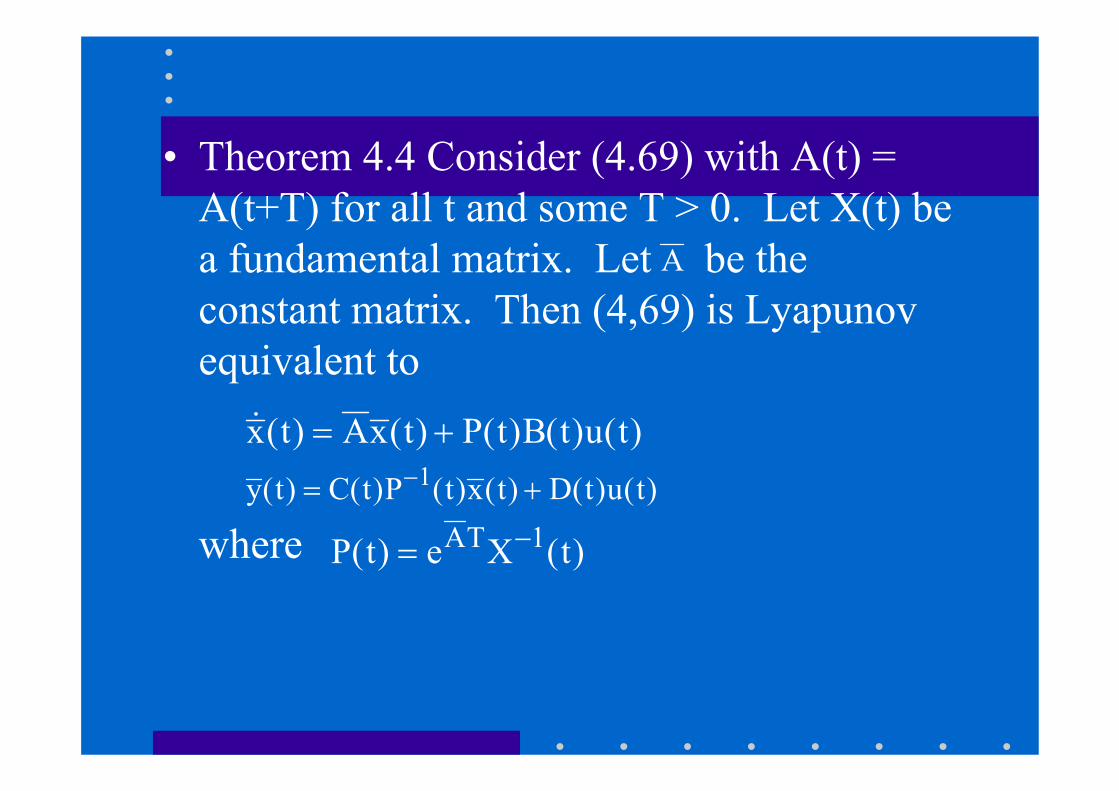
• Theorem 4.4 Consider (4.69) with A(t) = A(t+T) for all t and some T > 0. Let X(t) be a fundamental matrix. Let be the constant matrix. Then (4,69) is Lyapunovequivalent to

where

A

)t(u)t(B)t(P)t(xA)t(x +=&

)t(u)t(D)t(x)t(P)t(C)t(y 1 += −

)t(Xe)t(P 1TA −=

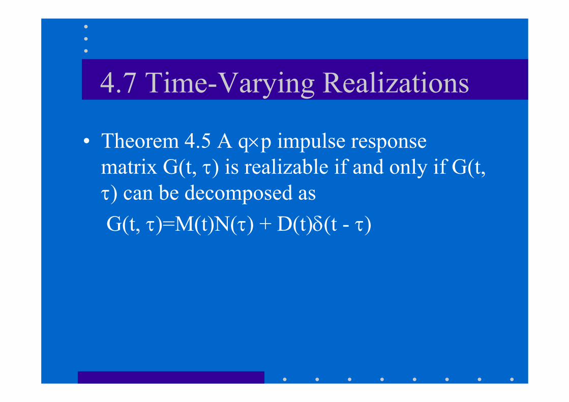
4.7 Time-Varying Realizations

• Theorem 4.5 A q×p impulse response matrix G(t, τ) is realizable if and only if G(t, τ) can be decomposed as G(t, τ)=M(t)N(τ) + D(t)δ(t - τ)