Linear Algebra Notesby

James L. Moseley

SPACE: THE FINAL FRONTIER

A SERIES OF CLASS NOTES TO INTRODUCE LINEAR AND NONLINEAR PROBLEMS TO ENGINEERS, SCIENTISTS, AND APPLIED MATHEMATICIANS

LINEAR CLASS NOTES:

A COLLECTION OF HANDOUTS

FOR

REVIEW AND PREVIEW

OF LINEAR THEORY

INCLUDING FUNDAMENTALS

OF

LINEAR ALGEBRA

by

James L. Moseley

Do not reproduce these notes without the expressed permission of Dr. James Moseley.

© 2012 James L. Moseley

CONTENTS

Chapter 0. Introductory Material

Chapter 1. Review of Elementary Algebra and Geometry in One, Two, and Three Dimensions

Chapter 2. Elementary Matrix Algebra

Chapter 3. Vector Spaces and Subspaces

Chapter 4. Introduction to Solving Linear Algebraic Equations

Chapter 5. Linear Operators, Span, Linear Independence, Basis Sets, and Dimension

Chapter 6. Preview of the Theory of Abstract Linear Equations of the First Kind

Chapter 7. Introduction to Determinants

Chapter 8. Inner Product and Normed Linear Spaces

Chapter 9. More on Matrix Inverses

A SERIES OF CLASS NOTES TO INTRODUCE LINEAR AND NONLINEAR PROBLEMS TO ENGINEERS, SCIENTISTS, AND APPLIED MATHEMATICIANS

LINEAR CLASS NOTES:A COLLECTION OF HANDOUTS FOR REVIEW AND PREVIEW

OF LINEAR THEORY INCLUDING FUNDAMENTALS OF

LINEAR ALGEBRA

CHAPTER 0

Introductory Material

1. Teaching Objectives for the Linear Algebra Portion of the Course

2. Sample Lectures for Linear Algebra

TEACHING OBJECTIVES for the

LINEAR ALGEBRA PORTIONof Math 251 (2-4 weeks)

1. Help engineering students to better understand how mathematicians do mathematics, including understanding the concepts of concrete and abstract spaces. 2. Know how to do matrix operations with real and complex matrices. This may require some remedial work in complex arithmetic including the conjugate of a complex number.3. Require that students memorize the definition of the abstract concept of a Vector (or Linear) Space as an abstract algebraic structure and that of a subspace of a vector space. The definition of a vector space includes the eight axioms for Vector Space Theory. The general definition of a Subspace in mathematics is a set with the same structure as the space. For a Vector Space, this requires closure of vector addition and multiplication by a scalar.4. Be able to solve for all three cases (unique solution, no solution, and infinte number Ax = b

of solutions). Understand what a problem is in mathematics, especially scalar and vector equations. 5. Develop some understanding of the definitions of Linear Operator, Span, Linear Independence, Basis, and Dimension. This need not be indepth, but exposure to all of the definitions is important. Understanding begins with exposure to the definitions. This orients students toward as a mapping problem and understanding dimension as an algebraic Ax = b

concept, helping them not to get stuck in 3-space.6. Know how to compute determinants by both using the Laplace expansion and by using Gauss elimination. 7. Know how to compute the inverse of a matrix. A formula for a 2x2 can be derived.8. Know the properties of a nonsingular (square) matrix and other appropriate theory (without proofs).

SAMPLE LECTURES FOR LINEAR ALGEBRA

We begin with an algebraic rather than a geometric approach to vectors. This will help theengineers not to get stuck in 3-space. If you start with geometry and then start talking about n-space, the engineers decide that what you are saying has nothing to do with engineering and quitlistening. “Help I’m stuck in three space and I can’t get out.”

DO NOT PRESENT IN CLASS ANY OF THE MATERIAL IN CHAPTER 1. Havethem read it on their own. This material provides background to help the students to convertfrom a geometric approach to an algebraic approach to vectors. This makes it easier to move onto 4,5,...n... dimensions but is not necessary to go over in class.

Lecture #1 “SPACE, THE FINAL FRONTIER”Handout#1 Page 1 and 2 (on one sheet of paper) of any old exam.

To a mathematician, a space is a set plus structure. There are two kinds: Concrete andAbstract. The number systems, NZQRC, are sets with structure and hence are spaces. However, we do not call them spaces, we call them number systems. We may begin with thePeano Postulates, and then construct successively the positive integers (natural numbers) N, theintegers Z,the rational numbers Q, and the reals R and the complexes C. However, in a realanalysis course, we follow Euclid and list the axioms that uniquely determine R. These fall intothree categories: the field (algebraic) axioms, the order axioms, and the least upper bound axiom(LUB). These are sufficient to determine every real number so that R is concrete (as are all thenumber systems). If we instead consider only the field axioms, we have the axioms for theabstract algebraic structure we call a field. We can define a field informally as a number systemwhere we can add, subtract, multiply, and divide (except by zero of course). (Do not confuse analgebraic field with a scalar or vector field that we will encounter later in Vector Calculus.) Sincean algebraic field is an abstract space, we give three examples: Q, R, and C. N and Z are notfields. Why?

A matrix is an array of elements in a field. Teach them to do matrix algebra with C aswell as R as entries. Begin with the examples on the old exam on page 1. That is, teach themhow to compute all of the matrix operations on the old exam. You may have to first teach themhow to do complex arithmetic including what the conjugate of a complex number is. Some willhave had it in high school, some may not. The True/False questions on page 2 of the old examprovide properties of Matrix Algebra. You need not worry about proofs, but for false statementssuch as “Matrix multiplication of square matrices is commutative” you can provide or have themprovide counter examples. DO NOT PRESENT THE MATERIAL IN CHAPTER 2 IN CLASS. It provides the proofs of the matrix algebra properties.

Lecture #2 VECTOR (OR LINEAR) SPACESHandout#2 One sheet of paper. On one side is the definition of a vector space from the notes. On the other side is the definition of a subspace from the notes.

Begin by reminding them that a space is a set plus structure. Then read them thedefinition of a vector space. Tell them that they must memorize this definition. This is oursecond example of an abstract algebraic space. Then continue through the notes giving themexamples of a vector space including Rn, Cn, matrices, and function spaces.

Then read them the definition of a subspace. Tell them that they must memorize this

definition. Stress that a subspace is a vector space in its own right. Why? Use the notes asappropriate, including examples (maybe) of the null space of a Linear Operator.

Lecture #3&4 SOLUTION OF Ax = b

Teach them how to do Gauss elimination. See notes. Start with the real 3x3 Example#1on page 8 of Chapter 4 in the notes. This is an example with exactly one solution. Then do theexample on page 15 with an arbitrary . Do both of the ‘s. One has no solution; one has anb

b

infinite number of solutions. Note that for a 4x4 or larger, geometry is no help. They will getgeometry when you go back to Stewart.

Lecture #5&6 REST OF VECTOR SPACE CONCEPTSGo over the definitions of Linear Operators, Span, Linear Independence, Basis Sets, andDimension. You may also give theorems, but no proofs (no time). Two examples of Linearoperators are T:Rn Rm defined by and the derivative D:A (R,R)A (R,R) where ifT(x) = Ax

fA (R,R) = {fF (R,R): f is analytic on R) and F (R,R) is the set of all real valued functions of areal variable, and we define D by . dfD(f) =

dx

Lecture #7 DETERMINANTS AND CRAMER’S RULETeach them how to compute determinants and how to solve using Cramer’s Rule.Ax = b

Lecture #8 INVERSES OF MATRICESTeach them how to compute (multiplicative) inverses of matrices. You can do any size matrix byaugmenting it with the (multiplicative) identity matrix I and using Gauss elimination. I do anarbitrary 2x2 to develop a formula for the inverse of a 2x2 which is easy to memorize.

This indicates two weeks of Lectures, but I usually take longer and this is ok. Try to get acrossthe idea of the difference in a concrete and an abstract space. All engineers need Linear Algebra. Some engineers need Vector Calculus. If we have to short change someplace, it is better theVector Calculus than the Linear Algebra. When you go back to Stewart in Chapter 10 and pickup the geometrical interpretation for 1,2, and 3 space dimensions, you can move a little faster soyou can make up some time. My first exam covers up through 10.4 of Stewart at the end of thefourth week. Usually, by then I am well into lines and planes and beyond.

A SERIES OF CLASS NOTES TO INTRODUCE LINEAR AND NONLINEAR PROBLEMS TO ENGINEERS, SCIENTISTS, AND APPLIED MATHEMATICIANS

LINEAR CLASS NOTES:A COLLECTION OF HANDOUTS FOR

REVIEW AND PREVIEW OF LINEAR THEORY

INCLUDING FUNDAMENTALS OF LINEAR ALGEBRA

CHAPTER 1

Review of Elementary Algebra and Geometry in

One, Two, and Three Dimensions

1. Linear Algebra and Vector Analysis

2. Fundamental Properties of the Real Number System

3. Introduction to Abstract Algebraic Structures: An Algebraic Field

4. An Introduction to Vectors

5. Complex Numbers, Geometry, and Complex Functions of a Complex Variable

Ch. 1 Pg. 1

Handout #1 LINEAR ALGEBRA AND VECTOR ANALYSIS Professor Moseley

As engineers, scientists, and applied mathematicians, we are interested in geometry fortwo reasons:1. The engineering and science problems that we are interested in solving involve time and space. We model time by R and (three dimensional) space using R3. However some problems can be idealized as one or two dimensional problems. i.e., using R or R2. We assume familiarity with R as a model for one dimensional space (Descartes) and with R2 as a model for two dimensional space (i.e., a plane). We assume less familiarity with R3 as a model of three space, but we do assume some.2. Even if the state variables of interest are not position in space (e.g., amounts of chemicals in a reactor, voltages, and currents), we may wish to draw graphs in two or three dimensions that represent these quantities. Visualization, even of things that are not geometrical, may provide some understanding of the process.It is this second reason (i.e., that the number of state variables in an engineering system of interestmay be greater than three) that motivates us to consider “vector spaces” of dimension greaterthan three. When speaking of a system, the term “degrees of freedom” is also used, but we willusually use the more traditional term “dimension” in a problem solving setting where noparticular application has been selected.

This leads to several definitions for the word “vector”;1. A physical quantity having magnitude and direction. (What your physics teacher told you.)2. A directed line segment in the plane or in 3-space.3. An element in R2 or R3 (i.e., an ordered pair or an ordered triple of real numbers).4. An element in Rn (i.e., an ordered n-tuple of real numbers).5. An element in Kn where K is a field (an abstract algebraic structure e.g., Q, R and C). 6. An element of a vector space (another abstract algebraic structure).

The above considerations lead to two separate topics concerning “vectors”.1. Linear Algebra.2. Vector Analysis

In Linear Algebra a “vector” in an n dimensional vector space may represent n statevariables and thus a system having n degrees of freedom. Although pictures of such vectors inone, two, and three dimensions may provide insight into the behavior of our system, these graphsneed have no geometrical meaning. A system having n degrees of freedom and requiring n statevariables resides in an n dimensional vector space which has no real geometrical meaning (e.g.,amounts of n different chemicals in a reactor, n voltages or currents, tension in n differentelements in a truss, flow rates in n different connected pipes, or amounts of money in n differentaccounts) . This does not diminish the usefulness of these vector spaces in solving engineering,science, and economic problems. A typical course in linear algebra covers topics in three areas:1. Matrix Algebra.2. Abstract Linear Algebra (Vector Space Theory).3. How to Solve a System of m Linear Algebraic Equations in n Unknowns.Although a model for the equilibrium or steady state of a linear system with n state variablesusually has n equations in n unknowns, little is gained and much is lost by a restriction to n

Ch. 1 Pg. 2

equations in n unknowns. Matrix algebra and abstract linear algebra (or vector space theory)provide the tools for understanding the methods used to solve m equations in n unknowns. Thebig point is that no geometrical interpretation of a vector is needed to make vectors in linearalgebra useful for solving engineering, scientific, and economic problems. A geometricalinterpretation is useful in one, two and three dimensions to help you understand what can happenand the “why’s” of the solution procedure, but no geometrical interpretation of a vector in “n”space is needed to make vectors in linear algebra useful for solving engineering, scientific,and economic problems.

In Vector Analysis (Vector Calculus and Tensor Analysis) we are very much interested inthe geometrical interpretation of our vectors (and tensors). Providing a mathematical model ofgeometrical concepts is the central theme of the subject. Interestingly, the “vector” spaces ofinterest from a linear algebra perspective are usually infinite dimensional as we are interested inphysical quantities at every point in physical space and hence have an infinite number of degreesof freedom and hence an infinite number of state variables for the system. These are oftenrepresented using functions rather than n-tuples of numbers as well as “vector” valued functions(e.g., three ordered functions of time and space) . We divide our system models into twocategories based on the number of variables needed to describe a state for our system:1. Discrete System Models having only a finite number of state variables. These are sometimes referred to as lumped parameter systems in engineering books. Examples are electriccircuits, systems of springs and “stirred” chemical reactors.2. Continuum System Models having an infinite number of state variables in one , two, or three physical dimensions. These are sometimes referred to as distributed parameter systems in engineering books. Examples are Electromagnetic Theory (Maxwell’s equations), Elasticity, and Fluid Flow (Navier-Stokes equations). One last point. Although the static or equilibrium problem for a discrete or lumped parameterproblem requires you to find values for n unknown variables, the dynamics problem requiresvalues for these n variables for all time and hence requires an infinite number of values. Again,these are usually given by n functions of time or equivalently by an n-dimensional time varying“vector”. (Note that here the term vector means n-tuple. When we use “vector” to mean n-tuple,rather than an element in a vector space, we will put it in quotation marks.)

Ch. 1 Pg. 3

Handout #2 FUNDAMENTAL PROPERTIES Professor MoseleyOF THE REAL NUMBER SYSTEM

Geometrically, the real numbers R can be put in one-to-one correspondence with a line inspace (Descartes). We call this the real number line and view R as representing onedimensional space. We also view R as being a fundamental model for time. However, we wish toalso view R mathematically as a set with algebraic and analytic properties. In this approach, wepostulate the existence of the set R and use axioms to establish the fundamental properties. Otherproperties are then developed using a theorem/proof/definition format. This removes the need toview R geometrically or temporally and allows us to algebraically move beyond three dimensions. Degrees of freedom is perhaps a better term, but dimension is standard in mathematics and wewill use it. We note that once a mathematical mode has been developed, although sometimesuseful for intuitive understanding, no geometrical interpretation of R is needed in the solutionprocess for engineering, scientific, and economic problems. We organize the fundamentalproperties of the real number system into several groups. The first three are the standardaxiomatic properties of R:

1) The algebraic (field) properties. (An algebraic field is an abstract algebraic structure. Examples are Q, R, and C. However, N and Z are not)2) The order properties. (These give R its one dimensional nature.)3) The least upper bound property. (This leads to the completeness property that insures that R has no “holes” and may be the hardest property of R to understand. R and C are complete, but Q is not complete)All other properties of the real numbers follow from these axiomatic properties. Being

able to “see” the geometry of the real number line may help you to intuit other properties of R. However, this ability is not necessary to follow the axiomatic development of the properties of R,and can sometimes obscure the need for a proof of an “obvious” property.

We consider other properties that can be derived from the axiomatic ones. To solveequations we consider

4)Additional algebraic (field) properties of R including factoring of polynomials. To solve inequalities, we consider:

5) Additional order properties including the definition and properties of the order relations <, >, , and . A vector space is another abstract algebraic structure. Application problems are often

formulated and solved using the algebraic properties of fields and vector spaces. R is not only afield but also a (one dimensional) vector space. The last two groups of properties of interestshow that R is not only a field and a vector space but also an inner product space and hence anormed linear space:

6) The inner product properties and 7) The norm (absolute value or length) properties.

These properties are of interest since the notion of length (norm) implies the notion of distanceapart (metric), and hence provides topological properties and allows for approximate solutions. They can be algebraically extended to two dimensions (R2), three dimensions (R3), n dimensions(Rn), and even infinite dimensions (Hilbert Space). There are many applications for vector

Ch. 1 Pg. 4

spaces of dimension greater than three (e.g., solving m linear algebraic equations in n unknownvariables) and infinite dimensional spaces (e.g., solving differential equations). In theseapplications, the term dimension does not refer to space or time, but to the degrees of freedomthat the problem has. A physical system may require a finite or infinite number of state variablesto specify the state of the system. Hence it would aid our intuition to replace the term dimensionwith the term degrees of freedom. On the other hand (OTOH), just as the real number line aids(and sometimes confuses) our understanding of the real number system, vector spaces in one two,and three dimensions can aid (and confuse) our understanding of the algebraic properties ofvector spaces.

ALGEBRAIC (FIELD) PROPERTIES. Since the set R of real numbers along with the binaryoperations of addition and multiplication satisfy the following properties, the system denoted bythe 5-tuple (R, +, .0,1) is an example of a field which is an abstract algebraic structure.

A1. x+y = y+x x,y R Addition is CommutativeA2. (x+y)+z = x+(y+z) x,y z R Addition is AssociativeA3. 0 R s.t. x+0 = x x R Existence of a Right Additive IdentityA4. x R w s.t. x+w = 0 Existence of a Right Additive InverseA5. xy = yx x,y R Multiplication is CommutativeA6. (xy)z = x(yz) x,y z R Multiplication is AssociationA7. 1 R s.t. x 1 = x x R Existence of a Right Multiplicative IdentityA8. x R s.t. x0 w R s.t. xw=1 Existence of a Right Multiplicative Inverse

A9. x(y+z) = xy + xz x,y z R Multiplication Distributes over Addition

There are other algebraic (field) properties which follow from these nine fundamental properties. Some of these additional properties (e.g., cancellation laws) are listed in high school algebrabooks and calculus texts. Check out the above properties with specific values of x, y, and z. Forexample, check out property A3 with x = π. Is π + 0 = π?

ORDER PROPERTIES. There exists the subset PR = R+ of positive real numbers that satisfies the following:

O1. x,y PR implies x+y PRO2. x,y PR implies xy PRO3. x PR implies -x PR

O4. x R implies exactly one of x = 0 or x PR or -x PR holds (trichotomy).

Note that the order properties involve the binary operations of addition and multiplication and aretherefore linked to the field properties. There are other order properties which follow from thefour fundamental properties. Some of these are listed in high school algebra books and calculustexts. The symbols <, >, <, and > can be defined using the set PR. For example, ab if (and onlyif) baPR{0}. The properties of these relations can then be established. Check out the aboveproperties with specific values of x and y. For example, check out property O1 with x = 2and y = π. Is + π positive?2

Ch. 1 Pg. 5

LEAST UPPER BOUND PROPERTY: The least upper bound property leads to the completeness property that assures us that the real number line has no holes. This is perhaps the most difficult concept to understand. It means that we must include the irrational numbers (e.g. π and ) with the rational numbers (fractions) to obtain all of the real numbers.2

DEFINITION. If S is a set of real numbers, we say that b is an upper bound for S if for each x S we have x < b. A number c is called a least upper bound for S if it is an upper bound for S and if c < b for each upper bound b of S.

LEAST UPPER BOUND AXIOM. Every nonempty set S of real numbers that has an upper bound has a least upper bound.

Check this property out with the set S = {x R: x2 < 2}. Give three different upper bounds for the set S. What real number is the least upper bound for the set S? Is it in the set S?

ADDITIONAL ALGEBRAIC PROPERTIES AND FACTORING. Additional algebraicproperties are useful in solving for the roots of the equation f(x) = 0 (i.e., the zeros of f) where fis a real valued function of a real variable. Operations on equations can be defined which result inequivalent equations (i.e., ones with the same solution set). These are called equivalentequation operations (EEO’s). An important property of R states that if the product of two realnumbers is zero, then at least one of them is zero. Thus if f is a polynomial that can be factoredso that f(x) = g(x) h(x) = 0, then either g(x) = 0 or h(x) = 0 (or both since in logic we use theinclusive or). Since the degrees of g and h will both be less than that of f, this reduces a hardproblem to two easier ones. When we can repeat the process to obtain a product of linear factors,we can obtain all of the zeros of f (i.e., the roots of the equation).

ADDITIONAL ORDER PROPERTIES. Often application problems require the solution ofinequalities. The symbols <, >, , and can be defined in terms of the set of positive numbers PR = R+ = {xR: x>0} and the binary operation of addition. As with equalities, operations oninequalities can be developed that result in equivalent inequalities (i.e., ones that have the samesolution set). These are called equivalent inequality operations (EIO’s).

ADDITIONAL PROPERTIES. There are many additional properties of R. We consider hereonly the important absolute value property which is basically a function.

x if x < 0x =

x if x 0

This function provides a norm, a metric, and a topology for R. Thus we can define limits,derivatives and integrals over intervals in R.

Ch. 1 Pg. 6

Handout #3 INTRODUCTION TO ALGEBRAIC STRUCTURES: Prof. MoseleyAN ALGEBRAIC FIELD

To introduce the notion of an abstract algebraic structure we consider (algebraic)fields. (These should not to be confused with vector and scalar fields in vector analysis.) Loosely, an algebraic field is a number system where you can add, subtract, multiply, and divide(except for dividing by zero of course). Examples of fields are Q, R, and C. Examples of otherabstract algebraic structures are: Groups, Rings, Integral Domains, Modules and Vector Spaces.

DEFINITION. Let F be a set (of numbers) together with two binary operations (which we calladdition and multiplication), denoted by + and (or juxtaposition), which satisfy the followinglist of properties.:

F1) x,y F x + y = y + x Addition is commutative F2) x,y F x + ( y + z ) = ( x + y ) + z Addition is associative F3) an element 0 F such that. x F, x + 0 = x Existence of a right additive identityF4) x F, a unique y F s.t. x + y = 0 Existence of a right We usually denote y by -x for each x in F. additive inverse for each elementF5) xy = yx x,y F Multiplication is commutative F6) x(yz) = (xy)z x,y,z F Multiplication is associative F7) an element 1 F such that 10 and x F, x1 = x Existence of a

a right multiplicative identityF8) x s.t. x0, a unique y F s.t. xy = 1 Existence of a right multiplicative inverse We usually denote y by (x-1) or (1/x) for each nonzero x in F. for each element except 0 F9) x( y + z ) = xy + xz x,y,z F (Multiplication distributes over addition)

Then the ordered 5-tuple consisting of the set F and the structure defined by the two operations ofaddition and multiplication as well as two identity elements mentioned in the definition, K = (F,+,,0,1), is an algebraic field.

Although technically not correct, we often refer to the set F as the (algebraic) field. Theelements of a field (i.e. the elements in the set F) are often called scalars. Since the letter F isused a lot in mathematics, the letter K is also used for a field of scalars. Since the rationalnumbers Q, the real numbers R, and the complex numbers C are examples of fields, it will beconvenient to use the notation K to represent (the set of elements for) any field K = (K,+,,0,1).

The properties in the definition of a field constitute the fundamental axioms for fieldtheory. Other field properties can be proved based only on these properties. Once we provedthat Q, R, and C are fields (or believe that someone else has proved that they are) then, by theprinciple of abstraction, we need not prove these properties for these fields individually, oneproof has done the work of three. In fact, for every (concrete) structure that we can establish as afield, all of the field properties apply.

We prove an easy property of fields. As a field property, this property must hold in everyalgebraic field. It is an identity and we use the standard form for proving identities.

THEOREM #1. Let K = (K,+,,0,1) be a field.. Then xK, 0 + x = x. (In English, this propertystates that the right identity element 0 established in F3 is also a left additive identity element.) Proof. Let xK. Then

Ch. 1 Pg. 7

STATEMENT REASON0 + x = x + 0 F1. Addition is commutative = x F3 0 is a rightr additive identity element.

(and properties of equality)Hence xK, 0 + x = x.

Q.E.D.

Although this property appears “obvious” (and it is) a formal proof can be written. This is whymathematicians may disagree about what axioms to select, but once the selection is made, theyrarely disagree about what follows logically from these axioms. Actually, the first four propertiesestablish a field with addition as an Abelian (or commutative) group (another abstract algebraicstructure). Group Theory, particularly for Abelian groups have been well studied bymathematicians. Also, if we delete 0, then the nonzero elements of K along with multiplicationalso form an Abelian group. We list some (Abelian) group theory properties as they apply tofields. Some are identities, some are not.

THEOREM #2. Let K = (K,+,,0,1) be a field. Then 1. The identity elements 0 and 1 are unique.2. For each nonzero element in K, its additive and multiplicative inverse element is unique.3. 0 is its own additive inverse element (i.e., 0 + 0 = 0) and it is unique, but it has nomultiplicative inverse element.4. The additive inverse of an additive inverse element is the element itself. (i.e., if a is theadditive inverse of a, then (a) = a ).5. (a + b) = a + b. (i.e., the additive inverse of a sum is the sum of their additive inverses.)6. The multiplicative inverse of a multiplicative inverse element is the element itself. (i.e., if a-1 isthe multiplicative inverse of a, then (a1)1 = a ).7. (a b)1 = a1 b1. (i.e., the multiplicative inverse of a product is the product of theirmultiplicative inverses.)8. Sums and products can be written in any order you wish.9. If a + b = a + c, then b = c. (Left Cancellation Law for Addition)10. If ab = ac and a 0, then b = c. (Left Cancellation Law for Multiplication.)

Ch. 1 Pg. 8

Handout #5 AN INTRODUCTION TO VECTORS Prof. Moseley

Traditionally the concept of a vector is introduced by physicists as a quantity such as forceor velocity that has magnitude and direction. Vectors are then represented geometrically bydirected line segments and are thought of geometrically. Modern mathematical treatmentsintroduce vectors algebraically as elements in a vector space. As an introductory compromise weintroduce two dimensional vectors algebraically and then examine the correspondence betweenalgebraic vectors and directed line segments in the plane. To define a vector space algebraically,we need a set of vectors and a set of scalars. We also need to define the algebraic operations ofvectors addition and scalar multiplication. Since we associate the analytic set R2 = {(x,y): x,y R} with the geometric set of points in a plane, we will use another notation, 2, for the set oftwo dimensional algebraic vectors.

SCALARS AND VECTORS. We define our set of scalars to be the set of real numbers R andour set of vectors to be the set of ordered pairs 2 = {[x,y]T: x,y R}. We use the matrixnotation [x,y]T (i.e.[x,y] transpose, see Chapter 2) to indicate a column vector to save space. (We could use row vectors, [x,y], but when we solve liear algebraqic equations we prefer columnvectors.) When writing homework papers it is better to use column vectors explicitly. We write

= [x,y]T and refer to x and y as the components of the vector .x x

VECTOR ADDITION. We define the sum of the vectors = [x1,y1]T and = [x2,y2]T x1

x2

as the vector + = [x1 + x2, y1 + y2]T. For example, [2,1]T + [5,2]T = [7,1]T. Thus we addx1 2x

vectors component wise.

SCALAR MULTIPLICATION. We define scalar multiplication of a vector = [x,y]T x

by a scalar α R by α = [α x, α y]T . For example, 3[2,1]T = [6,3]T. Thus we multiplyx

each component in by the scalar α. We define = [1, 0]T and = [ 0, 1]T so that every vector x i j

= [ x, y]T may be written uniquely as = x + y . x x i j

GEOMETRICAL INTERPRETATION. Recall that we associate the analytic set R2 = {(x,y): x,y R} with the geometric set of points in a plane. Temporarily, we use = (x,y)~xto denote a point in R2. We might say that the points in a plane are a geometric interpretation of R2. We can establish a one-to-one correspondence between the analytic set R2 and geometricalvectors (directed line segments). First consider only directed line segments which are positionvectors; that is, have their “tails” at the origin (i.e. at the point = (0,0) and their heads at some~0other point, say, the point = (x,y) in the plane R2 = {(x,y): x, yR}. Denote this set by G.~x

Position vectors are said to be “based at ”. If R2 is a point in the plane, then we let0 ~x 0 x

denote the position vector from the origin to the point . “Clearly” there exist a one-to-one~0 ~xcorrespondence between G and the set R2 of points in the plane; that is, we can readily identifyexactly one vector in G with exactly one point in R2. Now “clearly” a one-to-onecorrespondence also exists between the set of points in R2 and the set of algebraic vectors in 2. Hence a one-to-one correspondence exists between the set of algebraic vectors 2 and the set ofgeometric vectors G. In a traditional treatment, vector addition and scalar multiplication aredefined geometrically for directed line segments in G. We must then prove that the geometricdefinition of the addition of two directed line segments using the parallelogram law corresponds

Ch. 1 Pg. 9

to algebraic addition of the corresponding vectors in 2. Similarly for scalar multiplication. Wesay that we must prove that the two structures are isomorphic. It is somewhat simpler to definevector addition and scalar multiplication algebraically on 2 and think of G as a geometricinterpretation of the two dimensional vectors. One can then develop the theory of vectorswithout getting bogged down in the geometric proofs to establish the isomorphism. We canextend this isomorphism to R2. However, although we readily accept adding geometric vectors inG and will accept with coaxing adding algebraic vectors in 2 , we may baulk at the idea ofadding points in R2. However, the distinction between these sets with structure really justamounts to an interpretation of ordered pairs rather than an inherent difference in themathematical objects being considered. Hence from now on, for any of these we will use thesymbol R2 unless there is a philosophical reason to make the distinction. Reviewing, we have

2 G R2

where we have used the symbol to denote that there is an isomorphism between these sets withstructure.

MAGNITUDE AND DIRECTION. Normally we think of directed line segments as being “free”vectors; that is, we identify any directed line segment in the plane with the directed line segmentin G which has the same magnitude (length) and direction. The magnitude of the algebraic

vector = [x,y]T 2 is defined to be = which, using Pythagoras, is thex x x y2 2

length of the directed line segment in G which is associated with . It is easy to show that thex

property (i.e. prove the theorem) α = α holds for all 2 and all scalars α. x x x

It is also easy to show that if 0 the vector / = (1/ ) has magnitude equalx x x x x

to one (i.e. is a unit vector). Examples of unit vectors are = [1, 0]T and = [ 0, 1]T. i j“Obviously” any nonzero vector = [x,y]T can be written as = where =

x x x u u x/ is a unit vector in the same direction as . That is, gives the direction of andx x u x

gives its magnitude. For example, = [ 3, 4]T = 5 [3/5, 4/5]T where = [3/5, 4/5]T andx x u

= 5. To make vectors in 2 more applicable to two dimensional geometry we canx

introduce the concept of an equivalence relation and equivalence classes. We say that anarbitrary directed line segment in the plane is equivalent to a geometrical vector in G if it has thesame direction and magnitude. The set of all directed line segments equivalent to a given vectorin G forms an equivalence class. Two directed line segments are related if they are in the sameequivalence classes. This relation is called an equivalence relation since all directed linesegments that are related can be thought of as being the same. The equivalence classes partitionthe set of all directed line segments into sets that are mutually exclusive whose union is all of thedirected line segments.

VECTORS IN R3. Having established an isomorphism between R2, 2, and G, we make nodistinction in the future and will usually use R2 for the set of vectors in the plane, the set of pointsin the plane and the set of geometrical vectors. The context will explain what is meant. A similardevelopment can be done algebraically and geometrically for vectors in 3-space. There is atechnical difference between the sets R×R×R = {(x,y,z): x, y, zR}, R2×R = {((x,y),z): x, y,zR}, and R×R2 = {(x,(y,z)): x, y, zR}, but they are all isomorphic and we will usually considerthem to be the same and denote all three by R3. Furthermore, similar to 2 dimensions, we will use R3 to represent: the set of ordered triples, the set of points in 3 dimensional space, the set of 3

Ch. 1 Pg. 10

dimensional position vectors given by = [x,y,z]T = x + y + z where = [1, 0, 0]T, = [x i j k i j

0, 1, 0]T, and = [ 0, 0, 1]T, and the set of any three dimensional geometric vectors denoted bykdirected line segments.

The same analytic (but not geometric) development can be done for 4,5,..., n to obtain theset Rn of n-dimensional vectors. Again, no “real” geometrical interpretation is available. Thisdoes not diminish the usefulness of n-dimensional space for engineering since, for example, itplays a central role in the theory behind solving linear algebraic equations (m equations in n unknowns) and the theory behind any system which has n state variables (e.g., springs, circuits,and stirred tank reactors). The important thing to remember is that, although we may usegeometric language for Rn, we are doing algebra (and/or analysis), and not geometry.

PROPERTIES THAT CAN BE EXTENDED TO HIGHER DIMENSIONS. There areadditional algebraic, analytic, and topological properties for R, R2, and R3 that deserve to belisted since they are easily extended from R, R2,R3 to R4,..., Rn,... and, indeed to the (countably)infinite dimensional Hilbert space. We list these in four separate categories: inner product, norm,metric, and topology. Topologists may start with the definition of a topology as a collection ofopen sets. However, we are only interested in topologies that come from metrics which comefrom norms.

INNER (DOT) PRODUCT PROPERTIES. For x1, x2R, define = x1x2. For =1 2x ,x 1x

[x1,y1]T = x1 + y1 , = [x2,y2]T = x2 + y2 R2, define = x1x2 + y1y2. For for =i j 2x i j 1 2x ,x

1x

[x1,y1,z1]T = x1 + y1 + z1 , = [x2,y2,z2]T = x2 + y2 + z2 R3 define = x1x2i j k 2x i j k 1 2x ,x

+ y1y2 + z1z2. Then in R, R2, and R3 and, indeed, in any (real) inner product space V, we have thefollowing (abstract) properties of an inner product:

IP1) x,y y,x x,y V

IP2) x y, z x,z y,z , , , ,x y z V R

IP3) x,x 0 if 0x

< x,x > = 0 if x = 0

Check these properties out using specific values of x, y, z, α, β. For example, check out property IP2 with α = 2, β = 4, x = 1, y = 3 and z = 5. First calculate the left hand side (LHS), then theright hand side (RHS). Are they the same? Is the property true for these values? Now do thesame when = [2,3]T = 2 + 3 , = [1,4]T = + 4 and α =2 and β = 3. Also try some1x i j 2x i jthree dimensional vectors.

The inner or dot product of two vectors in two and three dimensions is more oftendenoted by . We have used the “physics” notation in 2 and 3 dimensions since

x y x, y

(x,y) is used to denote the coordinates of a point in the plane R2 and (x,y,z) for a point in 3 space. Note that we do not use arrows over the “vectors” when we are in one dimension. In R2 and R3,the geometric definition of inner (dot) product is where is the norm1 2 1 2 cosx ,x x x (magnitude) (see below) of the vector and θ is the angle between the two vectors. In Rn, the

definition of the inner product is where andn

i ii=1

(x,y) = x y n1 2 n i i=1

x = (x , x ,..., x ) = x

Ch. 1 Pg. 11

. Note we have moved to algebraic notation (no geometric interpretation is available). ni i=1

y = y

NORM (ABSOLUTE VALUE OR LENGTH) PROPERTIES. For xR, define , i.e., the absolute value of the number. For = [x,y]T = x + y R2,2x,x x x x xx x i j

define . For for = [x,y,z]T = x + y + z define . Then in2 2x x y x i j k 2 2 2x x y z

R, R2, and R3 and, indeed, in any normed linear space V, we have the following (abstract)properties of a norm:

N1) 0 if 0x x

= 0 if x = 0x = 0 if x = 0

N2) x x x V, R

N3) x, y R (Triangle Inequality)x, y Vx + y x + y

Check these properties out using specific values of x and α. For example check out property 2 with α = -3 and x = 2. That is, calculate the left hand side (LHS), then the righthand side (RHS). Are they the same? Is the property true for these values? Now check out theseproperties for two and three dimensional vectors.

In R, R2 and R3, the norm is the geometric magnitude or length of the vector. In Rn, the

norm of the vector is defined to be . ni i=1

x = x n2

ii=1

= xx

METRIC. For x1, x2R, define . For = [x1,y1]T = x1 + y1 , = [x2,y2]T1 2 1 2)(x ,x x x 1x i j 2x

= x2 + y2 R2, define . For = [x1,y1,z1]T i j 2 21 2 1 21 2 1 2) = (x - x ) + (y - y )(x ,x x x

1x

= x1 + y1 + z1 , = [x2,y2,z2]T = x2 + y2 + z2 R3 definei j k 2x i j k. Then in R, R2, and R3, and indeed, in any2 2 2

1 2 1 2 1 21 2 1 2) ) ( ) ( )(x ,x x x x x y y z z

metric space V, we have the following (abstract) properties of a metric:

M1 ρ(x,y) > 0 if x y

ρ(x,y) = 0 if x = y

M2 ρ(x,y) = ρ(y,x) x,y V

M3 ρ(x,z) ρ(x,y) +ρ(y,z) x,y,z V

In R, R2 and R3, the metric is the geometric distance between the tips of the positionvectors. In Rn, the metric of the vectors , Rn is defined to be n

i i=1x = x n

i i=1y = y

. A metric yields a definition of limit. Although in Rn with n > 3,n

2i i

i=1

( = (x - y )x,y) x y

this in not geometric, it does provides a measure for evaluating approximate solutions toengineering problems having n state variables. This also allows for the concept of a sequence ofapproximate solutions that converges to the exact solution in engineering problems.

Ch. 1 Pg. 12

TOPOLOGY. A topology is a collection of (open) sets having certain properties. Intuitively, anopen set is one that does not contain any of its boundary points. For example, open intervals areopen sets in the usual topology for R. Disks that do not contain any boundary points are opensets in R2. Balls which do not contain any boundary points are open sets in R3. Similarly for Rn,but no geometry. Topologists characterize continuity in terms of open sets.

Ch. 1 Pg. 13

Handout # 5 COMPLEX NUMBERS, GEOMETRY, AND COMPLEX Prof. MoseleyFUNCTIONS OF A COMPLEX VARIABLE

To solve z2 + 1 = 0 we "invent" the number i with the defining property i2 = ) 1. (Electrical engineers use j instead if i.) We then “define” the set of complex numbers as C ={x+iy:x,yR}. Then z = x+iy is known as the Euler form of z and z = (x,y)C = {(x,y):x,yR}is the Hamilton form of z where we identify C with R2 (i.e., with points in the plane). If z1 =x1+iy, and z2 = x2+iy2, then z1+z2 =df (x1+x2) + i(y1+y2) and z1z2 =df (x1x2-y1y2) + i(x1y2+x2y2). Using these definitions, the nine properties of addition and multiplication in the definition of anabstract algebraic field can be proved. Hence the system (C, + ,,0,1) is an example of an abstractalgebraic field. Computation of the product of two complex numbers is made easy using theEuler form and your knowledge of the algebra of R, the FOIL (first, outer, inner, last) method,and the defining property i2 = 1. Hence we have (x1+iy1)(x2+iy2) = x1x2+x1iy2 + iy1y2 + i2y1y2 =x1x2 + i (x1y2 + y1y2) y1y2 = (x1x2 y1y2) + i (x1y2+x2y1). This makes evaluation of polynomialfunctions easy.

EXAMPLE #1. If f(z) = (3 + 2i) + (2 + i)z + z2, then f(1+i) = (3 + 2i) + (2 + i)(1 + i) + (1 + i)2 = (3 + 2i) + (2 + 3i + i2) + (1 + 2i + i2)

= (3 + 2i) + (2 + 3i 1) + (1 + 2i 1) = (3 + 2i) + (1 + 3i) + ( 2i ) = 4 + 7i

Division and evaluation of rational functions is made easier by using the complex conjugate. Wealso define the magnitude of a complex number as the distance to the origin in the complex plane.

DEFINITION #1. If z = x+iy, then the complex conjugate of z is given by = x iy. Also thezmagnitude of z is z = .x y2 2

THEOREM #1. If z,z1,z2C, then a) = + , b) = , c) z2= , d) =z. z + z1 2 z1 z2 z z1 2 z1 z2 z z z

REPRESENTATIONS. Since each complex number can be associated with a point in the(complex) plane, in addition to the rectangular representation given above, complex numberscan be represented using polar coordinates.

z = x + iy = r cos θ + i sin θ = r (cos θ + i sin θ) = r θ (polar representation)

Note that r = z. You should be able to convert from Rectangular form to Polar form and viceversa. For example, 2 π/4 = + i and 1 + i = 2 π/3 . Also, if z1 = 3 + i and 2 2 3

z2 = 1 + 2i, then = = = = = =z1z2

z1z2

z2z2

z1

z2

z22

(3 i)(1 2i)

(1 22 )

(3 6i i 2i2 )(1 4)

(3- 2 i)5 7 1

575

i

EXAMPLE # 2 If f(z) = , evaluate f(4+i).z (3 i)z (2 i)

Ch. 1 Pg. 14

Solution. f(4+i)) = = = (4 + i) (3 i)(4 + i) (2 i)

(7 + 2i)(6 + 3i)

(7 + 2i)(6 + 3i)

(6 - 3i)(6 - 3i)

= = = i = i(42 + 6) + (12 - 21)i(36 +9)

48 - 9i45

4845

945

1615

15

THEOREM #2. If z1 = r1θ1 and z2 = r2θ2, then a) z1 z2 = r1 r2 θ1 + θ2 , b) If z20, then

= θ1 θ2 , c) z12 = r1

22θ1 , d) z1n = r1

nnθ1 .z1z2

1

2

rr

EULER’S FORMULA. By definition ei θ =df cos θ + i sin θ. This gives another way to write complex numbers in polar form. z = 1 + i = 2(cos π/3 + i sin π/3 ) = 2 π/3 = 2e i π / 33 z = + i = 2 (cos π/4 + i sin π/4 ) = 2 π/4 = e i π / 42 2

More importantly, it can be shown that this definition allows the extension of exponential, logarithmic, and trigonometric functions to complex numbers and that the standard properties hold. This allows you to determine what these extensions should be and to evaluate these functions.

EXAMPLE #6. If f(z) = (2 + i) e (1 + i) z , find f(1 + i).Solution. First (1 + i) (1 + i) = 1 + 2i + i2 = 1 + 2i -1 = 2i. Hencef(1 + i) = (2 + i) e2i = (2 + i)( cos 2 + i sin 2) = 2 cos 2 + i ( cos 2 + 2 sin 2 ) + i2 sin 2

= 2 cos 2 - sin 2 + i ( cos 2 + 2 sin 2 ) (exact answer) 2(- 0.4161468)- (0.9092974)+ i (-0.4161468 +2 (0.9092974)) = -1.7415911 + i(1.4024480) (approximate answer)

How do you know that -1.7415911 + i(1.4024480) is a good approximation to 2 cos 2 - sin 2 + i( cos 2 + 2 sin 2 ) ? Can you give an expression for the distance between these two numbers?

In the complex plane, ez is not one-to-one. Restricting the domain of ez to the strip R×(-π,π] ) {(0,0)}, in the complex plane, we can define Ln z as the (compositional) inverse function of ez with this restricted domain. This is similar to restricting the domain of sin x to [-π/2, π/2] to obtain sin -1 x (Arcsin x) as its (compositional) inverse function.

EXAMPLE #7. If f(z) = Ln [(1 + i) z] , find f(1 + i).Solution. First (1 + i) (1 + i) = 1 + 2i + i2 = 1 + 2i -1 = 2i. Now let w = x + iy = f(1 + i) where x,y R. Then w = x + iy = Ln 2i. Since Ln z is the (compositional) inverse of the function of ez, we have that 2i = exp(x + iy) = e x ei y = ex ( cos y + i sin y ). Equating real and imaginary parts we obtain ex cos y = 0 and ex sin y = 2 so that cos y = 0 and hence y = ±π/2. Now ex sin π/2 = 2 yields x = ln 2, but ex sin(- π/2) = 2 implies ex = -2. Since this is impossible, we have the unique solution f(1 + i) = ln 2 + i (π/2). We check by direct computation using Euler’s formula: exp[ ln 2 + i(π/2) ] = e ln 2 ei (π/2) = 2 ( cos (π/2) + i sin (π/2) ) = 2i.This is made easier by noting that if z = x + iy = re i θ, then Ln z = Ln(r e i θ) = ln r + i θ.

Letting e i z = cos z + i sin z we have e -i z = cos z + i sin(-z) = cos z - i sin z. Adding we obtain cos z = (e i z + e -i z )/2 which extends cosine to the complex plane. Similarly sin z = (e i z - e -i z )/2i.

Ch. 1 Pg. 15

EXAMPLE #8. If f(z) = cos [(1 + i)z] , find f(1 + i).Solution. First recall (1 + i) (1 + i) = 1 + 2i + i2 = 1 + 2i 1 = 2i. Hencef(1 + i) = cos (2i) = (ei 2i + e i(-2i) /2 = (e -2 + e 2)/2 = cosh 2 (exact answer)

3.762195691. (approximate answer)How do you know that 3.762195691 is a good approximation to cosh 2 ? Can you give anexpression for the distance between these two numbers (i.e., cosh 2 and 3.762195691)?

It is important to note that we represent C geometrically as points in the (complex) plane. Hence the domain of f:CC requires two dimensions. Similarly, the codomain requires twodimensions. Hence a "picture” graph of a complex valued function of a complex variable requiresfour dimensions. We refer to this a s a geometric depiction of f of Type 1. Hence we can notvisualize complex valued function of a complex variable the same way that we do real valuedfunction of a real variable. Again, geometric depictions of complex functions of a complexvariable of Type 1 (picture graphs) are not possible. However, other geometric depictions arepossible. One way to visualize a complex valued function of a complex variable is what issometimes called a “set theoretic” depiction which we label as Type 2 depictions. We visualizehow regions in the complex plane (domain) get mapped into other regions in the complex plane(codomain). That is, we draw the domain as a set (the complex z-plane) and then draw the w =f(z) plane. Often, points in the z-plane are labeled and their images in the w-plane are labeled withthe same or similar notation. Another geometric depiction (of Type 3) is to let f(z) = f(x+iy) =u(x,y) + iv(x,y) and sketch the real and imaginary parts of the function separately. Instead of drawing three dimensional graphs we can draw level curves which we call a Type 4depiction. If we put these level curves on the same z-plane, we refer to it as a Type 5 depiction.

Ch. 1 Pg. 16

A SERIES OF CLASS NOTES TO INTRODUCE LINEAR AND NONLINEAR PROBLEMS TO ENGINEERS, SCIENTISTS, AND APPLIED MATHEMATICIANS

LINEAR CLASS NOTES:A COLLECTION OF HANDOUTS FOR

REVIEW AND PREVIEW OF LINEAR THEORY

INCLUDING FUNDAMENTALS OF LINEAR ALGEBRA

CHAPTER 2

Elementary Matrix Algebra

1. Introduction and Basic Algebraic Operations

2. Definition of a Matrix

3. Functions and Unary Operations

4. Matrix Addition

5. Componentwise Matrix Multiplication

6. Multiplication by a Scalar

7. Dot or Scalar Product

8. Matrix Multiplication

9. Matrix Algebra for Square Matrices

10. Additional Properties

Ch. 2 Pg. 1

Handout No. 1 INTRODUCTION AND Professor MoseleyBASIC ALGEBRAIC OPERATIONS

Although usually studied together in a linear algebra course, matrix algebra can bestudied separately from linear algebraic equations and abstract linear algebra (Vector SpaceTheory). They are studied together since matrices are useful in the representation and solution oflinear algebraic equations and yield important examples of the abstract algebraic structure calleda vector space. Matrix algebra begins with the definition of a matrix. It is assumed that youhave some previous exposure to matrices as an array of scalars. Scalars are elements of anotherabstract algebraic structure called a field. However, unless otherwise stated, the scalar entries inmatrices can be assumed to be real or complex numbers (Halmos 1958,p.1). The definition of amatrix is followed closely by the definition of basic algebraic operations (computationalprocedures) which involve the scalar entries in the matrices (e.g., real or complex numbers) aswell as possibly additional scalars. These include unary, binary or other types of operations.

Some basic operations which you may have previously seen are:1. Transpose of a matrix.2. Complex Conjugate of a matrix.3. Adjoint of a matrix. (Not the same as the Classical Adjoint of a matrix.)4. Addition of two matrices of a given size.5. Componentwise multiplication of two matrices of a given size (not what is usually called multiplication of matrices). 6. Multiplication of a matrix (or a vector) by a scalar (scalar multiplication).7. Dot (or scalar) product of two column vectors (or row vectors) to obtain a scalar. Also called an inner product. (Column and row vectors are one dimensional matrices.)8. Multiplication (perhaps more correctly called composition) of two matrices with the right sizes (dimensions).

A unary operation is an operation which maps a matrix of a given size to another matrixof the same size. Unary operations are functions or mappings, but algebraists and geometersoften think in terms of operating on an object to transform it into another object rather than interms of mapping one object to another (already existing) object. Here the objects being mappedare not numbers, they are matrices. That is, you are given one matrix and asked to computeanother. For square matrices, the first three operations, transpose, complex conjugate, andadjoint, are unary operations. Even if the matrices are not square, the operations are stillfunctions.

A binary operation is an operation which maps two matrices of a given size to a thirdmatrix of the same size. That is, instead of being given one matrix and being asked to computeanother, you are given two matrices and asked to compute a third matrix. Algebraist think ofcombining or transforming two elements into a new element. Addition and componentwisemultiplication (not what is usually called matrix multiplication), and multiplication of squarematrices are examples of binary operations. Since on paper we write one element, the symbol forthe binary operation, and then the second element, the operation may, but does not have to,depend on the order in which the elements are written. (As a mapping, the domain of a binaryoperation is a cross product of sets with elements that are ordered pairs.) A binary operation

Ch. 2 Pg. 2

that does not depend on order is said to be commutative. Addition and componentwisemultiplication are commutative; multiplication of square matrices is not.

This may be the first you have become aware that there are binary operations inmathematics that are not commutative. However, it is not the first time you have encountered anon-commutative binary operation. Instead of thinking of subtraction as the inverse operation ofaddition (which is effected by adding the additive inverse element), we may think of subtraction asa binary operation which is not commutative (a b is not usually equal to b a). However, thereis another fundamental binary operation on (R,R) that is not commutative. If f(x) = x2 and g(x)= x + 2, it is true that (f+g)(x) = f(x) + g(x) = g(x) + f(x) = (g+f)(x) xR so that f+g = g+f. Similarly, (fg)(x) = f(x) g(x) = g(x) f(x) = (gf)(x)xR so that fg = gf. However, (fg)(x) =f(g(x)) = f( x + 2) = (x + 2)2, but (gf)(x) = g(f(x)) = g(x2) = x2 + 2 so that fg gf. Hence thecomposition of functions is not commutative.

When multiplying a matrix by a scalar (i.e., scalar multiplication), you are given a matrixand a scalar, and asked to compute another matrix. When computing a dot (or scalar) product,you are given two column (or row) vectors and asked to compute a scalar.

EXERCISES on Introduction and Basic Operations

EXERCISE #1. True or False.

_____ 1. Computing the transpose of a matrix is a binary operation._____ 2. Multiplying two square matrices is a binary operation._____ 3. Computing the dot product of two column vectors is a binary operation.

Halmos, P. R.1958, Finite Dimensional Vector Spaces (Second Edition) Van Nostrand ReinholdCompany, New York.

Ch. 2 Pg. 3

Handout #2 DEFINITION OF A MATRIX Prof. Moseley

We begin with an informal definition of a matrix as an array of scalars. Thus an m×nmatrix is an array of elements from an algebraic field K (e.g.,real or complex numbers) which has m rows and n columns. We use the notation Km×n for the set of all matrices over the field K. Thus, R3x4 is the set of all 3x4 real matrices and C2x3 is the set of all 2x3 matrices of complexnumbers. We represent an arbitrary matrix over K by using nine elements:

= = [ aij ] Kmxn (1)Amxn

1,1 1,2 1,n

2,1 2,2 2,n

m,1 m,1 m,n

a a aa a a

a a a

Recall that an algebraic field is an abstract algebra structure. R and C as well as Q are examplesof algebraic fields. Nothing essential is lost if you think of the elements in the matrices as real orcomplex numbers in which case we refer to them as real or complex matrices. Parentheses aswell as square brackets may be used to set off the array. However, the same notation should beused within a given discussion (e.g., a homework problem). That is, you must be consistent inyour notation. Also, since vertical lines are used to denote the determinant of a matrix (it isassumed that you have had some exposure to determinants) they are not acceptable to denotematrices. (Points will be taken off if your notation is not consistent or if vertical lines are used fora matrix.) Since Kmxn for the set of all matrices over the field K, Rmxn is the set of all real matricesand Cmxn is the set of all complex matrices. In a similar manner to the way we embed R in C andthink of the reals as a subset of the complex numbers, we embed Rmxn in Cmxn and, unless toldotherwise, assume Rmxn Cmxn. In fact, we may think of Cmxn as Rmxn + i Rmxn so that every complex matrix has a real and imaginary part. Practically, we simplyexpand the set where we are allowed to choose the numbers ai j , i = 1, ..., m and j = 1, ..., n.

The elements of the algebraic field, ai j , i = 1, ..., m and j = 1, ..., n, (e.g., real or complexnumbers) are called the entries in (or components of) A. To indicate that ai j is the element inA is the ith row and jth column we have also used the shorthand notation A = [aij]. We mightalso use A = (aij). The first subscript of ai j indicates the row and the second subscript indicates the column. This is particularly useful if there is a formula for ai j . We say that the size or dimension of the matrix is m×n and use the notation to indicate that A is a matrix of size A

mxn

m×n. The entries in A will also be called scalars. For clarity, it is sometimes useful to separatethe subscripts with a comma instead of a space. For example we might use a12,2 and ai+3,i+j insteadof a12 2 and ai+3 i+j.

Ch. 2 Pg. 4

EXAMPLES. = and are examples of rational matrices.3x3A

1 3/2 47 2 61 8 0

B 1/3, 2/5, 3

= , and = are examples of real (non-rational) matrices. A3x3

3 47 2 61 8 0

B3x1

1

4

e

, and = are examples of complex (non-real) A 1 i, 2, 3 2i B3x2

2i e + i3 / 4 + 3i 1.5

2e 7matrices.

As was done above, commas (instead of just spaces) are often used to separate the entries in 1×n matrices (often called row vectors). Although technically incorrect, this practice is acceptablesince it provides clarity.

COLUMN AND ROW VECTORS. An m×1 matrix (e.g., ) is often called a column 143

vector. We often use [1,4,3]T to denote this column vector to save space. The T stands fortranspose as explained later. Similarly, a 1×n matrix (e.g., [1, 4, 3]) is often called a row vector. This stems from their use in representing physical vector quantities such as position, velocity, andforce. Because of the obvious isomorphisms, we will often use Rn for the set of real columnvector Rn×1 as well as for the set of real row vectors R1×n. Similarly conventions hold for complexcolumn and row vectors and indeed for Kn, Kn×1, and K1×n. That is, we use the term “vector”even when n is greater than three and when the field is not R. Thus we may use Kn for a finitesequence of elements in K of length n, no matter how we choose to write it.

EQUALITY OF MATRICES. We say that two matrices are equal if they are the same; that is, ifthey are identical. This means that they must be of the same size and have the same entries incorresponding locations. (We do not use the bracket and parenthesis notation within the samediscussion. All matrices in a particular discussion must use the same notation.)

A FORMAL DEFINITION OF A MATRIX. Since R and C are examples of an (abstract)algebraic structure called a field (not to be confused with a vector field considered in vectoranalysis), we formally define a matrix as follows: An m×n matrix A over the (algebraic) field K(usually K is R or C) is a function from the set D = {1,...,. m} × {1, ..., n} to the set K (i.e.,A: D K). D is the cross product of the sets {1,...,. m} and {1, ..., n}. Its elements are ordered pairs (i,j) where i{1,...,. m} and j{1, ..., n}. The value of the function A at the point(i.j) D is denoted by aij and is in the codomain of the function. The value (i.j) in the domain thatcorresponds to aij is indicated by the location of aij in the array. Thus the array gives the values of

Ch. 2 Pg. 5

the function at each point in the domain D. Thus the set of m×n matrices over the field K is theset of functions (D,K) which we normally denote by Km×n. The set of real m×n matrices is Rm×n

= (D,R) and the set of complex m×n matrices is Cm×n = (D,C).

EXERCISES on Definition of a Matrix

EXERCISE #1. Write the 2×3 matrices whose entries are: (a) aij = i+j, (b) aij = (3i + j2)/2, (c) aij = [πi + j].

EXERCISE #2. Write the 3×1 matrices whose entries are given by the formulas in Exercise 1.

EXERCISE # 3. Choose x and y so that A = B if:

(a) and

(b)

(c)

(d)

Ch. 2 Pg. 6

Handout No. 3 FUNCTIONS AND UNARY OPERATIONS Professor Moseley

Let K be an arbitrary algebraic field. (e.g. K = Q, R, or C). Nothing essential is lost ifyou think of K as R or C. Recall that we use Kmxn to denote the set of all matrices with entries in K that are of size (or dimension) mxn (i.e. having m rows and n columns). We first define thetranspose function that can be applied to any matrix A Kmxn. It maps Kmxn to Knxm. We thendefine the (complex) conjugate function from Cmxn to Cmxn. Finally, we define the adjointfunction (not the same as the classical adjoint) from Cmxn to Cnxm. We denote an arbitrary matrixA in Kmxn by using nine elements.

= = [ aij ] Kmxn (1)Amxn

a a aa a a

a a a

1,1 1,2 1,n

2,1 2,2 2,n

m,1 m,1 m,n

TRANSPOSE.

DEFINITION #1. If = [ ai j ] Kmxn, then = [ ] Knxm is defined by = a j i formxnA

nxm

TA ~aij~aij

i=1,...,n, j=1,...,m. AT is called the transpose of the matrix A. (The transpose of A is obtained byexchanging its rows and columns.) The transpose function maps (or transforms) a matrix in Kmxn to (or into) a matrix in Knxm. Thus for the transpose function T, we have T: Kmxn Knxm..

Note that we have not just defined one function, but rather an infinite number of functions,one for each set Kmxn. We have named the function T, but we use AT instead of T(A) for theelement in the codomain Knxm to which A is mapped. Note that, by convention, the notation

= [ aij ] means that aij is the entry in the ith row and jth column of A: that is, unless otherwisemxnA

specified, the order of the subscripts (rather than the choice of index variable ) indicates the rowand column of the entry. Hence [ aji ] .

nxm

TA

EXAMPLE. If , then . If , the . If1 2 3

A = 4 5 67 8 9

T

1 4 7A = 2 5 8

3 6 9

1 iB = 3 + i 2i

5 1+ i

T 1 3 + i 5B =

i 2i 1+ i

A is given by (1) above, then AT = . Note that this makes the rows and

1,1 2,1 n,1

1,2 2,2 n,2

1,m 2,m n,m

a a aa a a

a a a

columns hard to follow.

Ch. 2 Pg. 7

PROPERTIES. There are lots of properties, particularly if K = C but they generally involve otheroperations not yet discussed. Hence we give only one at this time. We give its proof using thestandard format for proving identities in the STATEMENT/REASON format. We representmatrices using nine components, the first , second, and last components in the first, second, andlast rows. We refer to this as the nine element method. For many proofs involving matrixproperties, the nine element method is sufficient to provide a convincing argument.

THEOREM #1. For all A Km×n = the set of all m×n complex valued matrices, ( AT )T = A.

Proof: Let

= = [ aij ] Kmxn (1)Amxn

1,1 1,2 1,n

2,1 2,2 2,n

m,1 m,1 m,n

a a aa a a

a a a

Then by the definition of the transpose of A we have

= = Knxm (2)Amxn

T

1,1 2,1 m,1

1,2 2,2 m,2

1,n 2,n m,nnxm

a a aa a a

a a a

[a ]i, j~

where . We now show (AT)T = A using the standard procedure for proving identities in~a aji, j j,ithe STATEMENT/REASON format.

STATEMENT REASON

1,1 1,2 1,n

2,1 2,2 2,n

T

mxn

m,1 m,2 m,n

a a aa a a

A

a a a

TT

T

Definition of A (using the nine element representation) (Notation)

Definition of transpose

1,1 2,1 m,1

1,2 2,2 m,2

1,n 2,n m,n

a a aa a a

a a a

T

Ch. 2 Pg. 8

= Definition of transpose

1,1 1,2 1,n

2,1 2,2 2,n

m,1 m,2 m,n

a a aa a a

a a a

= A Definition of A

Since A was arbitrary, we have for all A Kmxn that ( AT )T = A as was to be proved.Q.E.D.

Thus, if you take the transpose twice you get the original matrix back. This means that thefunction or mapping defined by the operation of taking the transpose is in some sense, its owninverse operation. (We call such functions or mappings operators.) If f: Km×n Km×n is definedby f(A) = AT, then f1(B) =BT. However, ff 1 unless m=n. That is, taking the transpose of asquare matrix is its own inverse function.

DEFINITION #2. If A Kn×n (i.e. A is square) and A = AT, then A is symmetric.

COMPLEX CONJUGATE.

DEFINITION #3. If = [ aij ] Cmxn, then = [ ] Cmxn. The (complex)mxnA

mxnA ija

conjugate function maps (or transforms) a matrix in Cmxn to (or into) a matrix in Cmxn. Thus forthe complex conjugate function C we have C: Cmxn Cmxn..

That is, the entry in the ith row and jth column is for 1,...,n, j=1,...,m. (i.e. the complexijaconjugate of A is obtained by taking the complex conjugate componentwise; that is, by taking thecomplex conjugate of each entry in the matrix.) Again we have not just defined one function, butrather an infinite number of functions, one for each set Kmxn. We have named the function C, butwe use instead of C(A) for the element in the codomain Knxm to which A is mapped. NoteAthat unlike AT there is no problem in defining directly.A

PROPERTIES. Again, there are lots of properties but most of them involve other operations notyet discussed. We give two at this time.

THEOREM #2. For all A Cm×n = the set of all m×n complex valued matrices, = A. A

Thus if you take the complex conjugate twice you get the original matrix back. As with thetranspose, taking the complex conjugate of a square matrix is its own inverse function.

Ch. 2 Pg. 9

THEOREM #3. ( )T = . A A T

That is, the operations of computing the complex conjugate and computing the transposein some sense commute. That is, it does not matter which operation you do first. If A is square,then these two functions on Cn×n do indeed commute in the technical sense of the word.

ADJOINT.

DEFINITION #4. If = [ aij ] Cmxn, then * = ( )T Cnxm. The adjoint mxnA

mxnA A

function maps (or transforms) a matrix in Cmxn to (or into) a matrix in Knxm. Thus for the adjointfunction A, we have , A: Cmxn Cnxm..

That is, the entry in the ith row and jth column is for 1,...,n, j=1,...,m. (i.e. the adjoint of Ajiais obtained by taking the complex conjugate componentwise and then taking the transpose.) Again we have not just defined one function, but rather an infinite number of functions, one foreach set Cmxn. We have named the function A (using italics to prevent confusion with the matrixA, but we use A* instead of A(A) for the element in the codomain Cnxm to which A is mapped. . Note that having defined AT and , A* can be defined in terms of these two functions withoutAhaving to directly refer to the entries of A.

PROPERTIES. Again, there are lots of properties but most of them involve other operations. Hence we give only one at this time.

THEOREM #4. A* = .A T

That is, in computing A*, it does not matter whether you take the transpose or thecomplex conjugate first.

DEFINITION #4. If A* = A, then A is said to be a Hermitian matrix.

THEOREM #5. If ARn×n, then A is symmetric if and only if A is Hermitian.

Hermitian matrices (and hence real symmetric matrices) have nice properties; but morebackground is necessary before these can be discussed. Later, when we think of a matrix as(defining) an operator, then a Hermitian matrix is (defines) a self adjoint operator.

Ch. 2 Pg. 10

EXERCISES on Some Unary Matrix Operations

EXERCISE # 1. Compute the transpose of each of the following matrices

a) b) A = [1, ½ ] c) d) 1 2

A =3 4

1 i 1+ iA =

2 2 + i 0

πA = e

2

e)A=[π,2] f) g) h) i) A = [i,e,π]

iA = 2 + i

3

2 2iA =

0 1

0 01+ i 2 + i1 0

EXERCISE # 2. Compute the (complex) conjugate of each of the matrices in Exercise 1 above.

EXERCISE # 3. Compute the adjoint of each of the matrices in Exercise 1 above.

EXERCISE # 4. The notation B = [bi j ] defines the entries of an arbitrary m×n matrix B. Writeout this matrix as an array using a nine component representation (i.e, as is done in Equation (1). Now write out the matrix C = [cij] as an array. Now write out the matrix CT as an array using thenine component method.

EXERCISE # 5. Write a proof of Theorem #2. Since it is an identity, you can use the standardform for writing proofs of identities. Begin by defining the arbitrary matrix A. Represent it usingthe nine component method. Then start with the left hand side and go to the right hand side,justifying every step in a STATEMENT/REASON format.

EXERCISE # 6. Write a proof of Theorem #3. Since it is an identity, you can use the standardform for writing proofs of identities. Begin by defining the arbitrary matrix A. Represent it usingthe nine component method. Then start with the left hand side and go to the right hand side,justifying every step.

Ch. 2 Pg. 11

Handout #4 MATRIX ADDITION Professor Moseley

DEFINITION #1. Let A and B be m × n matrices in Km×n defined by

= = [aij], = = [bij] (1)Amxn

a a aa a a

a a a

1,1 1,2 1,n

2,1 2,2 2,n

m,1 m,1 m,n

Bmxn

b b bb b b

b b b

1,1 1,2 1,n

2,1 2,2 2,n

m,1 m,1 m,n

We define the sum of A and B by

= Kmxn (2)A Bmxn mxn

a + b a + b a + ba + b a + b a + b

a + b a + b a + b

1,1 1,1 1,2 1,2 1,n 1,n

2,1 2,1 2,2 2,2 2,n 2,n

m,1 m,1 m,1 m,1 m,n m,n

that is, A + B C [ci j ] where ci j = ai j + bi j for i = 1,..., m and j = 1,..., n.

We say that we add A and B componentwise. Note that it takes less space (but is notas graphic) to define the i,jth component (i.e., c i j ) of A + B = C then to write out the sum inrows and columns. Since m and n are arbitrary, in writing out the entries, we wrote only nineentries. However, these nine entries may give a more graphic depiction of a concept that helpswith the visualization of matrix computations. 3×3 matrices are often used to represent physicalquantities called tensors. Similar to referring to elements in Kn, Kn×1, and K1×n as “vectors” evenwhen n>3 and KR, we will refer to A = ai j (without parentheses or brackets) as tensor notationfor any matrix A even when A is not 3×3. Thus ci j = ai j + bi j defines the matrix ci j as the sum ofthe matrices ai j and bi j using tensor notation. (The Einstein summation convention is discussedlater, but it is not assumed unless so stated .)

As a mapping, + maps an element in Km×n × Km×n to an element in Km×n, + : Km×n × Km×n Km×n where Km×n × Km×n = {(A,B):A,BKm×n} is the cross product of Km×n

with itself. The elements in Km×n × Km×n are ordered pairs of elements in Km×n. Hence the orderin which we add matrices could be important. Part b of Theorem 1 below establishes that it isnot, so that matrix addition is commutative. Later we will see that multiplication of squarematrices is a binary operation that is not commutative so that the order in which we multiplymatrices is important.

Ch. 2 Pg. 12

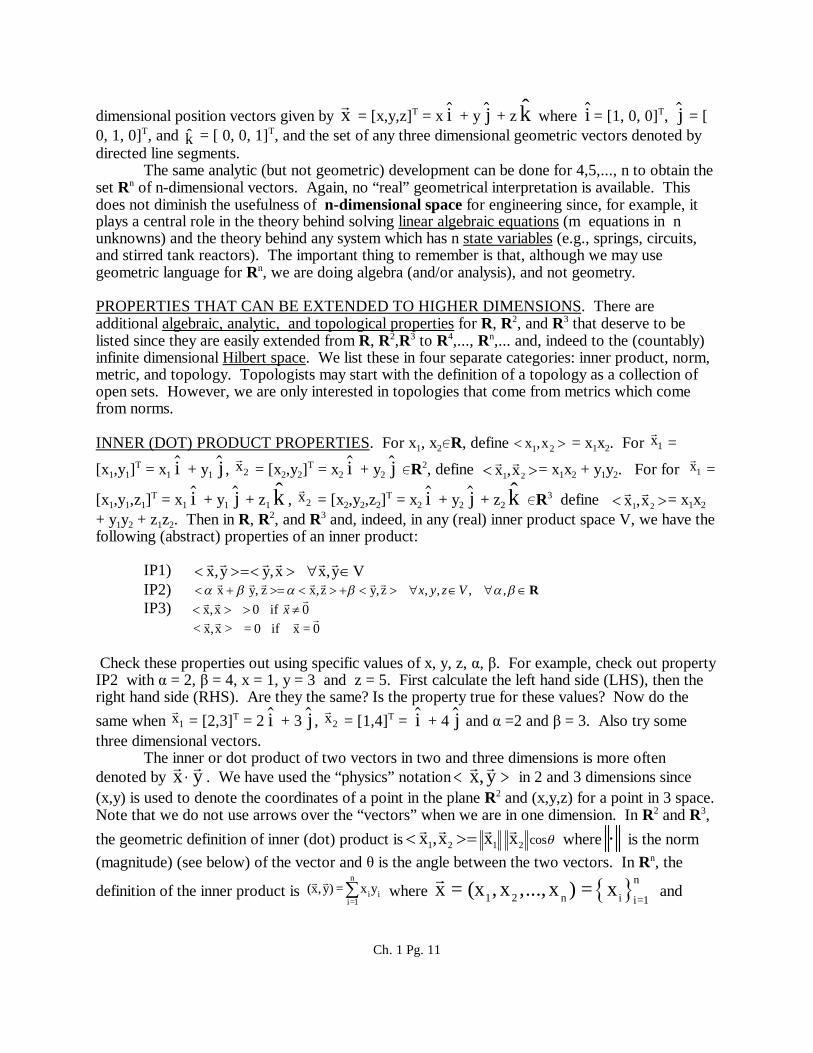
PROPERTIES. Since the entries in a matrix are elements of a field, the field properties can beused to prove corresponding properties of matrix addition. These properties are then given thesame names as the corresponding properties for fields.

THEOREM #1. Let A, B, and C be m × n matrices. Then

a. + ( + ) = ( + ) + (matrix addition is associative) (3)mxnA

mxnB

mxnC

mxnA

mxnB

mxnC

b. + = + (matrix addition is commutative) (4)mxnA

mxnB

mxnB

mxnA

THEOREM #2. There exists an m × n matrix Ο such that for all m × n matrices + = (existence of a right additive identity in Km×n).

mxnA

mxnO

mxnA

We call the right additive identity matrix the zero matrix since it can be shown to be the m × n matrix whose entries are all the zero element in the field K. (You may think of this element as thenumber zero in R or C.) To distinguish the zero matrix from the number zero we have denoted itby Ο; that is

= = [ 0 ] Kmxn (1)mxnO

0 0 00 0 0

0 0 0

THEOREM #3. The matrix Ο Kmxn is the unique additive identity element in Kmxn.

PARTIAL PROOF. The definition of and proof that Ο is an additive identity element is left to theexercises. We prove only that it is unique. To show that Ο is the unique element in Kmxn suchthat for all A Kmxn, A + Ο = Ο + A = A, we assume that there is some other matrix, say ΘKmxn that has the same property, that is, for all A Kmxn, A + Θ = Θ + A = A, and show that Θ =Ο. A proof can be written in several ways including showing that each element in Θ is the zeroelement of the field so that by the definition of equality of matrices we would have Θ = Ο. However, we can write a proof without having to consider the entries in Θ directly. Such a proveis considered to be more elegant. Although the conclusion, Θ = Ο is an equality, it is not anidentity. We will write the proof in the STATEMENT/REASON format, but not by starting withthe left hand side. We start with a known identity.

Ch. 2 Pg. 13

STATEMENT REASON

A Kmxn, A = Ο + A It is assumed that Ο has been established asan additive identity element for Kmxn.

Θ = Ο + Θ Let A= Θ in this known identity. = Ο Θ is assumed to be an identity so that for all

A Kmxn, A + Θ = Θ + A = A. This includesA = Ο so that Ο + Θ = Ο.

Since we have shown that the assumed identity Θ must in fact be Ο, (i.e., Θ = Ο), we have thatΟ is the unique additive identity element for Kmxn.

Q.E.D.

THEOREM #4. For every matrix , there exists a matrix, call it such that mxnA

mxnB

+ = (existence of a right additive inverse).mxnA

mxnB

mxnO

It is easily shown that B is the matrix containing the negatives of the entries in A. That is, if A = [aij] and B = [bij], then bij = aij. Hence we denote B by A. (This use of the minus signis technically different from the multiplication of a matrix by the scalar ) 1. Multiplication of amatrix by a scalar is defined later. Only then can we prove that these are the same.)

COROLLARY #5. For every matrix the unique right additive inverse matrix, call it , is mxnA

mxnA

= [ ] (Computation of the unique right additive inverse). mxnA ija

THEOREM #6. For every matrix , the matrix has the properties mxnA

mxnA

+ ( ) = + = . (-A is a (right and left) additive inverse).mxnA

mxnA

mxnA

mxnA

mxnO

Furthermore, this right and left inverse is unique.

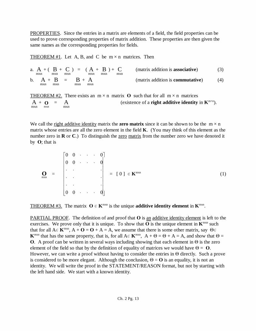
INVERSE OPERATION. We define subtraction of matrices by A - B = A + (-B). Thus to compute A ) B, we first find the additive inverse matrix for B (i.e., C = ) B where if C = [cij] and B = [bij], then cij = )bij). Then we add A to C = ) B. Computationally, if A = [aij] and B = [bij] then

Ch. 2 Pg. 14

= KmxnA Bmxn mxn

1,1 1,1 1,2 1,2 1,n 1,n

2,1 2,1 2,2 2,2 2,n 2,n

m,1 m,1 m,1 m,1 m,n m,n

a - b a - b a - ba - b a - b a - b

a - b a - b a - b

THEOREM #7. Let A, B Km×n. Then (A + B)T = AT + BT.

THEOREM #8. Let A, B Cm×n. Then the following hold:1) ( ) = + A B A B2) (A + B)* = A* + B*

EXERCISES on Matrix Addition

EXERCISE #1. If possible, add A to B (i.e., find the sum A + B) if

a) , b) A = [1,2] , B = [1,2,3]1 1 + iA =

2 2 i

0 2iB =

3 1 i

c) , d) , 0 1 + i

A = 2e 3

1 i i

1 + i 3

B = 2 0

0 1 i

2 + i

A = 0

1 i

2

2 + 2 i

B = 0

1 2 i

2

EXERCISE #2. Compute A+(B+C) (that is, first add B to C and then add A to the sumobtained) and (A+B)+C (that is, add A+B and then add this sum to C) and show that you get thesame answer if

a) , , b) , , 1 1 + iA =

2 2 i

0 2iB =

3 1 i

2 1 + iC =

1 1 i

0 1 + i

A = 2e 3

1 i i

1 + i 3

B = 2 0

0 1 i

2 2 + i

C = 3e 3

3 i i

, 2 + i

A = 0

1 i

2

2 + 2 i

B = 0

1 2 i

2

1 + i

C = 0

2 i

2

EXERCISE #3. Compute A+B (that is, add A to B) and B+A (that is, add B to A) and showthat you get the same answer if:

a) , b) , , 1 1 + iA =

2 2 i

0 2iB =

3 1 i

0 1 + i

A = 2e 3

1 i i

1 + i 3

B = 2 0

0 1 i

2 + i

A = 0

1 i

2

2 + 2 i

B = 0

1 2 i

2

EXERCISE #4. Can you explain in one sentence why both commutativity and associativity holdfor matrix addition? (Hint: They follow because of the corresponding properties for .)

(Fill in the blank)Now elaborate.

Ch. 2 Pg. 15

EXERCISE #5. Find the additive inverse of A if

a) c) A = [i,e,π]

EXERCISE # 6. Write a proof of Theorem #1. Since these are identities, use the standard formfor writing proofs of identities. Begin by defining arbitrary matrices A and B. Represent themusing at least the four corner entries. Then start with the left hand side and go to the right handside, justifying every step.

EXERCISE # 7. Write a proof of Theorem #2. Since it is an identity, you can use the standardform for writing proofs of identities. Begin by defining the arbitrary matrix A. Represent it usingat least the four corner entries. Then start with the left hand side and go to the right hand side,justifying every step.

EXERCISE # 8. Finish the proof of Theorem #3. Theorem #2 claims that O is a right additiveidenty, i.e., AKmxn we have the identity A+O = A. Thus we can use the standard form forwriting proofs of identities to show that O is also a left additive identity. Begin by defining thearbitrary matrix A. Represent it using at least the four corner entries. Then define the additiveinverse element O using at least the four corners. Then start with the left hand side and go to theright hand side, justifying every step. Hence O is an additive identity. We have shown uniquenessso that O is the additive identity element.

EXERCISE # 9. Write a proof of Theorem #4. Since it is an identity, you can use the standardform for writing proofs of identities. Begin by defining the arbitrary matrix A. Represent it usingat least the four corner entries. Then define the additive inverse element B = A = [aij] using atleast the four corners. Then start with the left hand side and go to the right hand side, justifyingevery step.

EXERCISE # 10. Write a proof of Corollary #5. You can use the standard form for writingproofs of identities to show that A is a right additive inverse. Then show uniqueness.

EXERCISE # 11. Write a proof of Theorem #6. Since it is an identity, you can use the standardform for writing proofs of identities.

EXERCISE # 12. Write a proof of Theorem #7. Since it is an identity, you can use the standardform for writing proofs of identities.

EXERCISE # 13. Write a proof of Theorem #8. Since these are identities, you can use thestandard form for writing proofs of identities.

Ch. 2 Pg. 16

Handout #5 COMPONENTWISE MATRIX MULTIPLICATION Professor Moseley

Componentwise multiplication is not what is usually called matrix multiplication. Although not usually developed in elementary matrix theory, it does not deserve to be ignored.

DEFINITION #1. Let A and B be m × n matrices in Km×n defined by

= = [aij], = = [bij] (1)Amxn

a a aa a a

a a a

1,1 1,2 1,n

2,1 2,2 2,n

m,1 m,1 m,n

Bmxn

b b bb b b

b b b

1,1 1,2 1,n

2,1 2,2 2,n

m,1 m,1 m,n

Then we define the componentwise product of A and B by

= Kmxn (2)A Bmxn mxn

a b a b a ba b a b a b

a b a b a b

1,1 1,1 1,2 1,2 1,n 1,n

2,1 2,1 2,2 2,2 2,n 2,n

m,1 m,1 m,1 m,1 m,n m,n

that is, A B C [cij] where cij = aij bij for i = 1,..., m and j = 1,..., n.

We say that we multiply A and B componentwise. Note that it takes less space (but isnot as graphic) to define the i,jth component (i.e., ci j ) of C = A B then to write out theproduct in rows and columns. Even in writing out the entries we were terse since we wrote onlynine entries of the array. Again, since this nine element technique often gives a more graphicdepiction of a concept, it will often be used to help with the visualization of matrix computations.

PROPERTIES. Since the entries in a matrix are elements of a field, the field properties can beused to prove corresponding properties for componentwise matrix multiplication.

THEOREM #1. Let A, B, and C be m × n matrices. Thena. ( ) = ( ) (componentwise matrix mult. is associative) (3)A

mxnB

mxnC

mxnAmxn

Bmxn

Cmxn

b. = (componentwise matrix mult. is commutative) (4)Amxn

Bmxn

Bmxn

Amxn

Ch. 2 Pg. 17

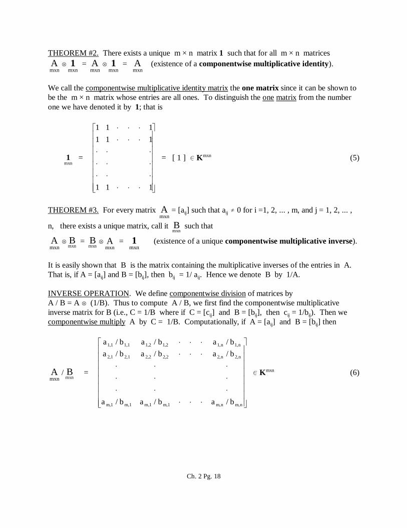
THEOREM #2. There exists a unique m × n matrix 1 such that for all m × n matrices = = (existence of a componentwise multiplicative identity).A

mxn1

mxnAmxn

1mxn

Amxn

We call the componentwise multiplicative identity matrix the one matrix since it can be shown tobe the m × n matrix whose entries are all ones. To distinguish the one matrix from the numberone we have denoted it by 1; that is

= = [ 1 ] Kmxn (5)1mxn

1 1 11 1 1

1 1 1

THEOREM #3. For every matrix = [aij] such that aij 0 for i =1, 2, ... , m, and j = 1, 2, ... ,Amxn

n, there exists a unique matrix, call it such that Bmxn

= = (existence of a unique componentwise multiplicative inverse).Amxn

Bmxn

Bmxn mxn

A 1mxn

It is easily shown that B is the matrix containing the multiplicative inverses of the entries in A. That is, if A = [aij] and B = [bij], then bij = 1/ aij. Hence we denote B by 1/A.

INVERSE OPERATION. We define componentwise division of matrices by A / B = A (1/B). Thus to compute A / B, we first find the componentwise multiplicativeinverse matrix for B (i.e., C = 1/B where if C = [cij] and B = [bij], then cij = 1/bij). Then wecomponentwise multiply A by C = 1/B. Computationally, if A = [aij] and B = [bij] then

/ = Kmxn (6)Amxn

Bmxn

a / b a / b a / ba / b a / b a / b

a / b a / b a / b

1,1 1,1 1,2 1,2 1,n 1,n

2,1 2,1 2,2 2,2 2,n 2,n

m,1 m,1 m,1 m,1 m,n m,n

Ch. 2 Pg. 18

EXERCISES on Componentwise Matrix Multiplication

EXERCISE #1. If possible, multiply componentwise A to B (i.e., find the componentwise product A cm B) if

a) b) A = [1,2] , B = [1,2,3]

c) d)

EXERCISE #2. Compute A cm (B cm C) (that is, first componentwise multiply B and C andthen componentwise multiply A and the product obtained) and ( A cm B ) cm C (that is, firstcomponentwise multiply A and B and then componentwise multiply the product obtained withC) and show that you get the same answer if

a)

b)

EXERCISE #3. Compute AB and BA and show that you get the same answer if:

a) b)

EXERCISE #4. Can you explain in one sentence why commutativity and associativity hold forcomponentwise matrix multiplication? (Hint: They follow because of the correspondingproperties for .)

(Fill in the blank, then elaborate)

EXERCISE #5. If possible, find the componentwise multiplicative inverse of A if

a) c) A = [i,e,π]

EXERCISE # 6. Write a proof of Theorem #1. Since these are identities, use the standard formfor writing proofs of identities. Begin by defining arbitrary matrices A and B. Represent themusing at least the four corner entries. Then start with the left hand side and go to the right handside, justifying every step.

EXERCISE # 7. Write a proof of Theorem #2. Since it is an identity, you can use the standard

Ch. 2 Pg. 19

form for writing proofs of identities. Begin by defining the arbitrary matrix A. Represent it usingat least the four corner entries. Then start with the left hand side and go to the right hand side,justifying every step.

EXERCISE # 8. Write a proof of Theorem #3. Since it is an identity, you can use the standardform for writing proofs of identities. Begin by defining the arbitrary matrix A. Represent it usingat least the four corner entries. Then define the additive inverse element B = -A = [-aij] using atleast the four corners. Then start with the left hand side and go to the right hand side, justifyingevery step.

Ch. 2 Pg. 20

Handout No.6 MULTIPLICATION BY A SCALAR Professor Moseley

DEFINITION #1. Let be an m×n matrix and α a scalar ( α K where K is a field):Amxn

= = [aij] Kmxn, α K (e.g., K = R or K = C) (1)Amxn

1,1 1,2 1,n

2,1 2,2 2,n

m,1 m,1 m,n

a a aa a a

a a a

then we define the product of α and A (called multiplication by a scalar, but not scalarproduct) by

α = = [ α aij ] Kmxn (1)Amxn

a a aa a a

a a a

1,1 1,2 1,n

2,1 2,2 2,n

m,1 m,1 m,n

that is, αA C = [cij] where cij = αaij for i = 1,..., m and j = 1,..., m. That is, we multiply eachcomponent in A by α. Again defining an arbitrary component cij of αA takes less space but isless graphic, that is, does not give a good visualization of the operation. However, you shouldlearn to provide that visualization, (i.e., look at cij = αaij and visualize each component beingmultiplied by α, for example, the nine element graphic above or the four corner graphic.) Sometimes we place the scalar on the right hand side (RHS): αA =α[aij] = [aij]α = Aα.

PROPERTIES. The following theorems can be proved.

THEOREM #1. Let A be an m×n matrix and 1 be the multiplicative identity in the associatedscalar field K (e.g., 1 R or 1 C), then 1A = A.

THEOREM #2. Let A and B be an m×n matrix and α and β be scalars in K(e.g., α,β R or α,β C), thena. α(βA) = (αβ)A (Note the difference in the meaning of the two sets of parentheses.)b. (α + β)A = (αA) + (βA) (Note the difference in the meaning of the two plus signs.)c. α(A+B) = (αA) + (βB) (What about parentheses and plus signs here?)

Ch. 2 Pg. 21

INVERSE OPERATION. If α is a nonzero scalar, the division of a matrix A by the scalar α isdefined to be multiplication by the multiplicative inverse of the scalar. Thus A/α = (1/α) A.

THEOREM #3. Let A, B Cm×n. Then the following hold:1) (αA)T = α AT

2)αA = αA3) (αA)* = α A*

EXERCISES on Multiplication by a Scalar

EXERCISE #1. Multiply A by the scalar α if

a) α = 2 and b) α = 2+i and A = [1,2] c) α = 1 and 1 1 + iA =

2 2 i

0 1 + i

A = 2e 3

1 i i

d) α =1 /2 and 2 + i

A = 0

1 i

2

EXERCISE #2. Compute (αA)T (that is, first multiply α by A and take the transpose) and then α AT (that is, multiply α by A transpose) and show that you get the same answer if

a) α = 2 and b) α = 2+i and A = [1,2] c) α = 1 and 1 1 + iA =

2 2 i

0 1 + i

A = 2e 3

1 i i

d) α = 1/2 and 2 + i

A = 0

1 i

2

EXERCISE #3. Compute (that is, multiply α by A and then compute the complex conjugate)αAand then compute (that is, compute and then and then multiply by ) and thenαA A α Ashow that you get the same answer if:

a) α = 2 and b) α = 2+i and A = [1,2] c) α = 1 and 1 1 + iA =

2 2 i

0 1 + i

A = 2e 3

1 i i

d) α = ½ and 2 + i

A = 0

1 i

2

Ch. 2 Pg. 22

Handout No.7 DOT OR SCALAR PRODUCT Professor Moseley

DEFINITION #1. Let = [x1,x2,...,xn] and = [y1,y2,...,yn] be row vectors in R1×n or C1×n (wex y

could just as well use column vectors). Then define the scalar product of and byx y

= = x y x y + x y + ... + x y1 1 2 2 n n x yi

i 1

n

i

In R2 and R3, this is usually called the dot product. (In an abstract setting, this operation isusually called an inner product.)

PROPERTIES. The following theorem can be proved.

THEOREM #1. Let = [x1,x2,...,xn], = [y1,y2,...,yn], and = [z1,z2,...,zn] be row vectors in x y z

R1×n or C1×n; we could just as well use column vectors) and α be a scalar. Then

a. = = x

y y x

yx

b. (x y) z x y x z

c. = α ( )( x) y x

y

d. x x 0

x x 0 if and only if x = 0

The term inner product is used for an operation on an abstract vector space if it has all of the properties given in Theorem #1. Hence we have that the operation of scalar product defined above is an example of an inner product and hence R1×n and K1×n (and Rn×1 and Cn×1 and Rn andCn) are inner product spaces.

EXERCISES on Dot or Scalar Product.

EXERCISE #1. Compute ifx

y

a) b) c)[1,2,1], [2,3,1]x y [1,2,3,4], [2,4,0,1]x y

[1,0,1,0], [1,2,0,1]x y

EXERCISE #2. Compute ifx

y

a) b) [1 ,2 ,0,1], [1 ,2 ,0,1]x i i y i i [1 ,0,0, ], [1 ,2 ,0,1]x i i y i i

c) [1,0,1, ], [1 ,2 ,0,1]x i y i i

Ch. 2 Pg. 23

Handout #8 MATRIX MULTIPLICATION Professor Moseley

Matrix multiplication should probably be called matrix composition, but the term matrixmultiplication is standard and we will use it.

DEFINITION #1. Let = [ aij ], = [ aij ]. Then = AB = [ cij ] where .Amxp

Bpxn

Cmxn

c = a bij iki 1

p

kj

Although the definition of the product matrix C is given without reference to the scalar product, itis useful to note that the element cij is obtained by computing the scalar product of the ith row of Awith the jth column of B and placing this result in the ith row and jth column of C. Using tensor

notation, we may just write . If we adopt the Einstein summation convention ofc = a bij iki 1

p

kj

summing over repeated indices, then this may be written as cij =aik bkj. This assumes that thevalues of m, n, and p are known.

EXAMPLE.

=

1 2 10 2 51 3 1

0 3 21 -1 31 1 1

3 - 4 57 3 114 1 12

A B C

c11 = [-1,2,1][0,1,1] = [-1,2,1][0,1,1]T = (-1)(0) + (2)(1) + (1)(1) = 3

c12 = [-1,2,1][3,-1,1] = [-1,2,1][3,-1,1]T = (-1)(3) + (2)(-1) + (1)(1) = -4

SIZE REQUIREMENT: In order to take the dot product of the ith row of A with the jth columnof B, they must have the same number of elements. Thus the number of columns of A must be thesame as the number of rows of B.

A B Cnxp pxn nxm

THE SCALAR PRODUCT IN TERMS OF MATRIX MULTIPLICATION. The dot product oftwo row vectors in R1×n can be given in terms of matrix multiplication. Let = [x1,x2,...,xn] and

x= [y1,y2,...,yn] be row vectors in R1×n. Then y

Ch. 2 Pg. 24

= = = x y x y + x y + ... + x y1 1 2 2 n n x yii 1

n

i

x y1xn nx1

T

If and are defined as column vectors, we havex y

= = = x y 1 1 2 2 n nx y + x y + ... + x y x yi

i 1

n

i T

1xn nx1x y

Using tensor notation, including the Einstein summation convention, we have = xi yi.x y

PROPERTIES. For multiplication properties, we must first be sure that all of the operations arepossible. Note that unless A and B are square, we can not compute both AB and BA. Even forsquare matrices, AB does not always equal BA (except for 1×1's). However, we do have:

THEOREM #1. Let , , and be matrices so that the multiplications , Amxp

Bpxr rxn

CmxpA

pxrB

, ( ), and ( ) are all possible. Then Bpxr rxn

C Amxp

Bpxr rxn

C Amxp

Bpxr

Crxn

A(BC) = (AB)C. matrix multiplication is associative

THEOREM #2. Let , , and be matrices so that the multiplications , mxpA B

pxnCpxn

Amxp

Bpxn

and the additions + and + are all possible. Then Amxp

Cpxn

Bpxn

Cpxn

Amxp

Bpxn

Amxp

Cpxn

A(B + C) = AB + AC matrix multiplication on the left distributes over matric addition

Now let , , and be matrices so that the multiplications , , and theAmxp

Bmxp

Cpxn mxp pxn

A B Cpxn

Bmxp

Cpxn

additions + , and + are all possible. Then Amxp

Bmxp

Amxp

Cpxn

Bmxp

Cpxn

(A+B)C = AC + BC matrix multiplication on the right distributes over matric addition

THEOREM #3. Let and be matrices so that the matrix multiplications AB, (αA)B, and Amxp

Bpxn

A(αB) are all possible. Then (αA)B = A(αB) = α(AB).

Ch. 2 Pg. 25

EXERCISES on Matrix Multiplication

EXERCISE #1. If possible, multiply A times B (i.e., find the product AB) if

a) , b) , c) A = [1,2] , B = [1,2,3]1 1 + iA =

2 2 i

0 2iB =

3 1 i

1 1+ iA =

1 1 i

0 2iB =

3 1 i

d) , e) , f) , 0 1 + i

A = 2e 3

1 i i

1 + i 3

B = 2 0

0 1 i

1 0A =

2 2 i

0 2iB =

3 1 i

1 1 + iA =

2 0

0 2iB =

3 1 i

g) , h) , 2 + i

A = 0

1 i

2

2 + 2 i

B = 0

1 2 i

2

1 0 0A = 0 1 0

0 0 1

1 0 0B = 1+ i 1 0

0 0 1

EXERCISE #2. . If posible, compute A(B+C) (that is, first add B to C and then add A timesthis sum) and then AB and BC (that is, multiply AB and then BC) and then show that you get A(B+C) = AB +AC if

a) , , b) , 1 1 + iA =

2 2 i

0 2iB =

3 1 i

2 1 + iC =

1 1 i

0 1 + i

A = 2e 3

1 i i

1 + i 3

B = 2 0

0 1 i

2 2 + i

C = 3e 3

3 i i

Ch. 2 Pg. 26

Handout #9 MATRIX ALGEBRA FOR SQUARE MATRICES Professor Moseley

If A and B are square, then we can compute both AB and BA. Unfortunately, these maynot be the same.

THEOREM #1. If n >1, then there exists A, BR n×n such that AB BA. Thus matrixmultiplication is not commutative.

Thus AB=BA is not an identity. Can you give a counter example for n=2? (i.e. an examplewhere AB BA. See Exercise #2.)

DEFINITION #1. For square matrices, there is a multiplicative identity element. We definethe n×n matrix I by

= One's down the diagonal. Zero's everywhere else.Imxn

1 0 0

0 1 0

0 0 1

THEOREM #2. We have = = A Knxn Anxn

Inxn

Inxn

Anxn

Anxn

DEFINITION #2. If there exists B such that AB = I., then B is a right (multiplicative) inverseof A. If there exists C such that CA = I., then C is a left (multiplicative) inverse of A. If AB = BA = I, then B is a (multiplicative) inverse of A and we say that A is invertible. If B isthe only matrix with the property that AB = BA = I, then B is the inverse of A. If A has a uniqueinverse, then we say A is nonsingular and denote its inverse by A-1.

THEOREM #3. Th identity matrix is its own inverse.

Later (Chapter 9) we show that if A has a right and a left inverse, then it has a unique inverse. Hence we prove that A is invertible if and only if it is nonsingular. Even later, we show that if Ahas a right (or left) inverse, then it has a unique inverse. Thus, even though matrix multiplicationis not commutative, a right inverse is always a left inverse and is indeed the inverse. Somematrices have inverses; others do not. Unfortunately, it is usually not easy to look at a matrix anddetermine whether or not it has a (multiplicative) inverse.

THEOREM #4. There exist A, BR n×n such that AI is invertible and B has no inverse.

Ch. 2 Pg. 27

INVERSE OPERATION. If B has a right and left inverse then it is a unique inverse ((i.e., B-1

such that B-1B = BB-1 = I) and we can define Right Division AB-1 and Left Division B-1A of Aby B (provided B-1 exists). But since matrix multiplication is not commutative, we do not know

that these are the same. Hence is not well defined since no indication of whether we meanAB

left or right division is given.

EXERCISES on Matrix Algebra for Square Matrices

EXERCISE #1. True or False._____ 1. If A and B are square, then we can compute both AB and BA. _____ 2. If n >1, then there exists A, BR n×n such that AB BA. _____ 3. Matrix multiplication is not commutative. _____ 4. AB=BA is not an identity._____ 5. For square matrices, there is a multiplicative identity element, namely the n×n matrix I,

given by = .nxnI

1 0 0

0 1 0

0 0 1

_____ 6. A Knxn we have = = Anxn

Inxn

Inxn

Anxn

Anxn

_____ 7. If there exists B such that AB = I., then B is a right (multiplicative) inverse of A.

_____ 8. If there exists C such that CA = I., then C is a left (multiplicative) inverse of A._____ 9. If AB = BA = I, then B is a multiplicative inverse of A and we say that A is invertible. _____ 10. If B is the only matrix with the property that AB = BA = I, then B is the inverse of A._____ 11. If A has a unique inverse, then we say A is nonsingular and denote its inverse by A-1._____ 12. The identity matrix is its own inverse. _____ 13. If A has a right and a left inverse, then it has a unique inverse. _____ 14. A is invertible if and only if it is nonsingular. _____ 15. If A has a right (or left) inverse, then it has a unique inverse. _____ 16. Even though matrix multiplication is not commutative, a right inverse is always a left inverse._____ 17. The inverse of a matrix is unique._____ 18. Some matrices have inverses; others do not. _____ 19. It is usually not easy to look at a matrix and determine whether or not it has a (multiplicative) inverse._____ 20. There exist A, BR n×n such that AI is invertible and B has no inverse

Ch. 2 Pg. 28

EXERCISE #2. Let α= 2, A = , and B = . Compute the following:1 i 1 i

1 0

1 0i 1+ i

= ___________. AT =____________. A* = ____________. αA = ____________. A

A+B =____________. AB =_____________.

EXERCISE #3. Let α= 3, A = , and B = . Compute the following:i 1 i0 1+ i

1 0i 1+ i

= ___________. AT =____________. A* = ____________. αA = ____________. A

A+B =____________. AB =_____________.

EXERCISE #4. Solve where , , and . 2x2 2x1 2x1A x b

1 iA

i 1

xx

y

1b

i

EXERCISE #5. Solve where , , and 2x2 2x1 2x1A x b

1 iA

i 1

xx

y

1b

0

EXERCISE #6 Solve where , , and 2x2 2x1 2x1A x b

1 iA

i 0

xx

y

1b

i

Ch. 2 Pg. 29

Handout #10 ADDITIONAL MATRIX PROPERTIES Professor Moseley

Recall that if K is a field and Km×n is the set of all matrices over K, then the followingproperties of matrices are true.

THEOREM #1. Let Km×n is the set of all matrices over K. Then for all A, B, C Km×n , we have

1) A + ( B + C ) = ( A + B ) + C associativity of matrix addition 2) A + B = B + A commutativity of matrix addition 3) There exists a unique matrix O such that for every matrix A ε Km×n, A + O = A. 4) For each A ε Km×n, there exist a unique matrix called A such that A + (A) = O.

By using these properties, but without resorting to looking at the components of the matrices wecan prove

THEOREM #2. Let Km×n is the set of all matrices over K. Then for all A, B, C Km×n , we have

1) Ο + A = A.2) (B) + (A + B) = (A + B) + (B) = A3) (A + B) = (A) + (B). The additive inverse of a sum is the sum of the additive inverses.4) If A + B = A + C, then B = C This is the cancellation law (for addition).

The proofs of properties 1) to 3) in Theorem #2 are easily proved using the standard method forproving identities in STATEMENT/REASON format. However none of the reasons rely onlooking at the components of the matrices and hence do not rely directly on the properties of theunderlying field. Now note that property 4) in Theorem #2 is not an identity. The conclusion isan equality, but it is a conditional equality. Although one could write a somewhat contortedproof of the concluding equality (B = C) by starting with one side and using the substitutionaxiom of equality to achieve the other side, a better proof is achieved by simply adding the sameelement to both sides of the given equation. Explanations of why the element to be added exists(Property 4) in Theorem #4) and why you can add the same element to both sides of an equationand the result is the same (axiom of equality) are needed.

The properties given in Theorem #1 establish Km×n as a Abelian (or commutative)group. Since only these properties are needed to prove Theorem #2, we see that anymathematical structure having these properties (i.e., any commutative group) also has theproperties given in Theorem #2. We refer to both the defining properties given in Theorem #1and the resulting properties given in Theorem #2 as Abelian group properties.

Now recall that if K is a field and Km×n is the set of all matrices over K, then thefollowing additional properties of matrices have been proved.

THEOREM #3. Let Km×n is the set of all matrices over K. Then for all scalars α ß K and A, B Km×n , we have

Ch. 2 Pg. 30

1) α ( ß A ) = ( α ß ) A (Note that (α ß) indicates multiplication in the field K.)2) (α + ß) A = α A + ß A3) α (A + B ) = α A + α B4) 1 A = A .

The properties in Theorem #4 below are easy to prove directly for matrices. However, they canalso be proved by using the properties in Theorem #1 and Theorem #3 (and the properties inTheorem #2 since these can be proved using only Theorem #1), but without resorting to lookingat the components of the matrices.

THEOREM #4. Let Km×n is the set of all matrices over K. Then for all scalars α K and A Km×n , we have

1) 0A = Ο,2) α Ο = Ο,3) If α A = Ο, then either α = 0 or A = Ο.

The first two properties are identities and can be proved using the standard method. Some mightargue that such proofs can become contorted and other methods may be clearer. The third isneither an identity nor a conditional equality. The hypothesis is an equality, but the conclusionstates that there are only two possible reasons why the suppose equality could be true, either ofthe possibilities given in 1) or 2) (or both) but no others.

The properties given in Theorems #1 and #3 establish Km×n as a vector space (see Chapter2-3) over K. Since only properties in Theorems #1 and #3 are needed to prove Theorems #2 and#4, we see that any mathematical structure having the properties given in Theorems #1 and #3(i.e., any vector space) also has the properties given in Theorems #2 and 4. We refer to both thedefining properties given in Theorems #1 and #3 and the resulting properties given in Theorems#2 and #4 as vector space properties. We consider additional vector spaces in the next chapter. Later, we consider more propertiess of (multiplicative) inverses of square matrices.

Ch. 2 Pg. 31

EXERCISES on Additional Matrix Properties

EXERCISE #1. True or False._____ 1.If Km×n is the set of all matrices over K, then for all A, B, C Km×n , we have A + ( B + C ) = ( A + B ) + C._____ 2.If Km×n is the set of all matrices over K, then for all A, B, C Km×n , we have the associativity of matrix addition._____ 3.If Km×n is the set of all matrices over K, then for all A, B Km×n , we have A + B = B + A._____ 4.If Km×n is the set of all matrices over K, then for all A, B Km×n , we have the commutativity of matrix addition.

_____ 5.If Km×n is the set of all matrices over K, then we have that there exists a unique matrix O such that for every matrix A ε Km×n, A + O = A._____ 6.If Km×n is the set of all matrices over K, then we have that for each A ε Km×n, there exist a unique matrix called A such that A + (A) = O._____ 7. If Km×n is the set of all matrices over K, then we have Ο + A = A._____ 8. If Km×n is the set of all matrices over K, then (B) + (A + B) = (A + B) + (B) = A_____ 9. If Km×n is the set of all matrices over K, then for all A, B, C Km×n , we have (A + B) = (A) + (B)._____ 10. If Km×n is the set of all matrices over K, then for all A, B, C Km×n , we have that the additive inverse of a sum is the sum of the additive inverses._____ 11. If Km×n is the set of all matrices over K, then for all A, B, C Km×n , we have that if A + B = A + C, then B = C _____ 12. If Km×n is the set of all matrices over K, then A + B = A + C, then B = C is called the cancellation law for addition. _____ 13. Many of the properties of matrices are identies and can be proved using the STATEMENT/REASON format. _____ 14. Some of the properties of matrices do not rely on looking at the components of the matrices._____ 15. Some of the properties of matrices do not rely directly on the properties of the underlying field. _____ 16. Some of the properties of matrices are not identities._____ 17. Some of the properties of matrices are conditional equalities. _____ 18. Some of the properties of matrices can be proved by starting with one side and using the substitution axiom of equality to achieve the other side._____ 19. Sometimes a better proof of a matrix property can be obtained by simply adding the same element to both sides of a given equation. _____ 20. Sometimes a proofs of a matrix properties can be obtained by using properties of equality. _____ 21. A group is an abstract algebraic structure._____ 22. An Abelian group is an abstract algebraic structure._____ 23. A commutative group is an abstract algebraic structure.

Ch. 2 Pg. 32

_____ 24. The set of all matrices over a field K is a group._____ 25. The set of all matrices over a field K is an abelian group._____ 26. The set of all matrices over a field K is a commutative group._____ 27. The set of all matrices over a field K is a group._____ 28. If Km×n is the set of all matrices over K, then for all scalars α, ß K and A Km×n , we have α ( ß A ) = ( α ß ) A_____ 29. If Km×n is the set of all matrices over K, then for all scalars α, ß K and A,B Km×n , we have (α + ß) A = α A + ß A_____ 30. If Km×n is the set of all matrices over K, then for all scalars α K and A,B Km×n , we have α (A + B ) = α A + α B_____ 31. If Km×n is the set of all matrices over K, then for all A Km×n , we have 1 A = A ._____ 32. If Km×n is the set of all matrices over K, then for all A Km×n , we have 0A = Ο._____ 33. If Km×n is the set of all matrices over K, then for all all scalars α K we have α Ο = Ο._____ 34. If Km×n is the set of all matrices over K, then for all scalars α K and A Km×n , we have that if α A = Ο, then either α = 0 or A = Ο._____ 35. The set of all matrices over K is a vector space.

Ch. 2 Pg. 33

A SERIES OF CLASS NOTES TO INTRODUCE LINEAR AND NONLINEAR PROBLEMSTO ENGINEERS, SCIENTISTS, AND APPLIED MATHEMATICIANS

LINEAR CLASS NOTES:A COLLECTION OF HANDOUTS FOR

REVIEW AND PREVIEW OF LINEAR THEORY

INCLUDING FUNDAMENTALS OF LINEAR ALGEBRA

CHAPTER 3

Vector Spaces and Subspaces

1. Definition of a Vector Space

2. Examples of Vector Spaces

3. Subspace of a Vector Space

Ch. 3 Pg. 1

Handout #1 DEFINITION OF AN ABSTRACT VECTOR SPACE Professor Moseley

Abstract linear algebra begins with the definition of a vector space (or linear space) asan abstract algebraic structure. We may view the eight properties in the definition as thefundamental axioms for vector space theory. The definition requires knowledge of anotherabstract algebraic structure, a field where we can always add (and subtract) as well as multiply(and divide except for zero), but nothing essential is lost if you always think of the field (ofscalars) as being the real or complex numbers (Halmos 1958,p.1).

DEFINITION #1. A nonempty set of objects (vectors), V, together with an algebraic field (ofscalars) K, and two algebraic operations (vector addition and scalar multiplication) whichsatisfy the algebraic properties listed below (Laws of Vector Algebra) comprise a vector space. (Following standard convention, although technically incorrect, we will usually refer to the set ofvectors V as the vector space). The set of scalars K are usually either the real numbers R orthe complex numbers C in which case we refer to V as a real or complex vector space. Let

, , ε V be any vectors and α,ß ε K be any scalars. Then the following must hold:xy z

VS1) + ( + ) = ( + ) + Associativity of vector addition x y z x y z

VS2) + = + Commutativity of vector addition x y y x

VS3) There exists a vector , Existence of a right additive identity0

such that for every V, + = vector for vector addition x x

0 x

VS4) For each V, there exist a vector, denoted Existence of a right additive inverse x

by , such that + ( ) = . vector for each vector in V - xx - x

0

VS5) α (ß ) = ( αß) An associativity property for scalar x x

multiplication VS6) (α+ß) = (α ) + (ß ) A distributive property for scalar

x x xmultiplication and vector addition

VS7) α( + )= (α ) + (α ) Another distributive property for scalar x y x y

multiplication and vector addition VS8) 1 = A scaling property for scalar multiplication

x x

These eight properties are an essential part of the definition of a vector space. In abstract algebraterminology, the first four properties establish a vector space with vector addition as an Abelian (or commutative) group (another abstract algebraic structure). The last four properties giverules on how vector addition and scalar multiplication must behave together.

Although technically not correct, we often refer to the set V of vectors as the vectorspace. Thus the R, R2,R3, Rn, and Rm×n are referred to as real vector spaces and C, Cn, and Cm×n

as complex vector spaces. Also Q, Qn and Qm×n, and indeed, K, Kn, and Km×n for any field arereferred to as vector spaces. However, the definition of a vector space requires that its structurebe given. Thus to rigorously represent a vector space, we use a 5-tuple consisting of 1) the set ofvectors, 2) the set of scalars, 3) vector addition, 4) scalar multiplication, and 5) the zero vector

Ch. 3 Pg. 2

(which is the only vector required to be in all vector spaces). Thus V = (V, K, +, , ). (Since0

we use juxtaposition to indicate scalar multiplication, we have no symbol for multiplication of avector by a scalar and hence just leave a space.)

We consider some properties that hold in all vector spaces (i.e., they are vector spaceproperties like the original eight, but unlike the original eight, these follow from the original eightusing mathematical logic). Specific examples of vector spaces are given in the next handout. Once they have been shown to be vector spaces, it is not logically necessary to show directly thatthe properties in Theorems #1, #2 and #3 and Corollary #4 hold in these spaces. The propertieshold since we can show that they are vector space properties (i.e., they hold in an abstract vectorspace). However, you may wish to check out these properties in specific vector spaces (i.e.,provide a direct proof) to improve your understanding of the concepts. We start with an easyproperty for which we provide proof.

THEOREM #1. Let V = (V,K, +, , ) be a vector space. Then for all V, + = .0 x

0 x x

Proof. Let be any vector in V and let be the right additive identity for V (or V). Thenx

0

STATEMENT REASON + = + VS2. Vector addition is commutative0 x x 0

= VS3 is the right additive identity elementx

0

for V (or V ).Hence for all V, + = (i.e., is a left additive identity element as well as a right

x0 x x

0

additive identity element ).Q.E.D.

As in the proofs of any identity, the replacement of + by is effected by the property of0 x x

equality that says that in any equality, a quantity may be replaced by an equal quantity. (Note thatthe second equality is really + = as the LHS is assumed.) This proof is in some sense

0 x x

identical to the proof that for all xK, 0 + x = 0 for fields. This is because the property is really agroup theory property and vectors with vector addition (as well as scalars with scalar addition)form groups. We now list additional properties of a vector space that follow since the vectors ina vector space along with vector addition form a group. Since is both a left and right additive

0

identity element, we may now say that it is an additive identity element.

THEOREM #2. Let V be a vector space over the field K. (i.e., Let V = (V, K, +, , ) be a0

vector space.) Then 1. The zero vector is unique (i.e., there is only one additive identity element in V).2. Every vector has a unique additive inverse element.3. is its own additive inverse element (i.e., , + = ).0

0

0

0

4. The additive inverse of an additive inverse element is the element itself. (i.e., if - is the x

additive inverse of , then ( ) = ).x x x

Ch. 3 Pg. 3

5. ( = ) =( ) +( ). (i.e., the additive inverse of a sum is the sum of their additivex y x y

inverses.)6. Sums of vectors can be written in any order you wish.7. If + = + , then = . (Cancellation Law for Addition)

x y x z y z

We now give a theorem for vector spaces analogous to the one for fields that says that if theproduct of two numbers is zero, one of the numbers must be zero.

THEOREM #3. Let V be a vector space over the field K. (i.e., Let V = (V, K, +, , ) be a0

vector space. The scalars K may be thought of as either R or C so that we have a real orcomplex vector space, but V may not be thought of as Rn or Cn.)1. V, 0 = .

x x0

2. α K, α = 0

0

3. α K, V, α = implies either α = 0 or = .x x

0 x

0

COROLLARY#4 (Zero Product). Let V be a vector space over the field K. (K may be thoughtof is either R or C.) Let α K, V. Then α = if and only if α = 0 or = .

x x0 x

0

In the abstract algebraic definition of a vector space, vectors do not have a magnitude (or length). Later, we will discuss normed linear spaces where this structure is added to a vector space. However, the concept of direction, in the sense indicated in the following theorem, is in allvector spaces.

DEFINITION #2. Let V be a vector space over a field K. Two nonzero vectors , V are x y

said to be parallel if there is a scalar αK such that α = . (The zero vector has nox y

direction.) If V is a real vector space so that K=R, then two (non-zero) parallel vectors are in thesame direction if α>0, but in opposite directions if α<0.

EXERCISES on The Definition of an Abstract Vector Space

EXERCISE #1. True or False.For all questions, assume V is a vector space over a field K, , , V are any vectors and x

y zα,ß K are any scalars. _____ 1. The following property is an axiom in the definition of a vector space: VS) + ( + ) = ( + ) +

x y z x y z_____ 2. The following property is an axiom in the definition of a vector space: VS) + = +

x y y x_____ 3. The following property is an axiom in the definition of a vector space:

Ch. 3 Pg. 4

VS)There exists a vector such that for every V, + = 0 x x

0 x

_____ 4. The following property is an axiom in the definition of a vector space: VS) For each V, there exist a vector, denoted by , such that + ( ) = .

x - xx - x

0

_____ 5. The following property is an axiom in the definition of a vector space: VS) ) α (ß ) = ( αß)

x x_____ 6. The following property is an axiom in the definition of a vector space: VS) (α+ß) = (α ) + (ß )

x x x_____ 7. The following property is an axiom in the definition of a vector space: VS) α( + )= (α ) + (α )

x y x y_____ 8. The following property is an axiom in the definition of a vector space: VS) ) 1 =

x x_____ 9. In V, vector addition is associative._____ 10. In V, vector addition is commutative._____ 11.In V, for vector addition, there exist a right additive identity such that for every V,

x + = .

x0 x

_____ 12. For vector addition, every vector in V has a right additive inverse, denoted by , x

such that . x +( x) = 0

_____ 13. For all V, we have + = .x

0 x x

_____ 14. In V, the zero vector is unique._____ 15. There is only one additive identity element in V_____ 16. In V, every vector has a unique additive inverse element._____ 17. In V, is its own additive inverse element

0

_____ 18. The additive inverse of an additive inverse element is the element itself_____ 19. if is the additive inverse of in V, then ( ) = .

x x x x_____ 20. α K, V, α = implies either α = 0 or = .

x x0 x

0

Halmos, P. R.1958, Finite Dimensional Vector Spaces (Second Edition) Van Nostrand ReinholdCompany, New York.

Ch. 3 Pg. 5

Handout #2 EXAMPLES OF VECTOR SPACES Professor Moseley

If we define a specific set of vectors, a set of scalars and two operations that satisfy theeight properties in the definition of a vector space (i.e., the Laws or Axioms of Vector Algebra)we obtain an example of a vector space. Note that this requires that the eight properties given inthe definition of an (abstract) vector space be verified for the (concrete) example. We giveexamples of vector spaces, but the verification that they are indeed vector spaces is left to theexercises. We also give two ways of building a more complicated vector space from a givenvector space.

EXAMPLE #1. The set of sequences of a fixed length in a field K. Since we are not interestedin matrix multiplication at this time, we may think of them not only as sequences, but as columnvectors or as row vectors. When we consider linear operators, we wish them to be columnvectors and so we use this interpretation. For example, if K = R, we let

i) V = = Rnx1 Rnx

x

x

:x R, i 1,2,3,.., n

1

n

i

ii) The scalars are the real numbers R. iii) Vector addition is defined by

+ = . (i.e. Add componentwise as in matrix addition)

x

x

1

n

y

y

1

n

x y

x y

1 1

n n

iv) Scalar multiplication is defined by

α = . (i.e. Multiply each component in x by α as in multiplication

x

x

1

n

x

x

1

n

of a matrix by a scalar.)

Again, the space of row vectors: V = {(x1,...,xn): xiR, i = 1,...,n} = R1xn Rn is technicallydifferent from the space of column vectors. However, as far as being a vector space is concerned,the distinction is merely technical and not substantive. Unless we need to make use of the

Ch. 3 Pg. 6

technical difference we will denote both spaces by Rn. We refer to Rn as the space of n-tuples ofreal numbers whether they are written as row vectors or column vectors. If we wish to think ofrow vectors as n × 1 matrices, column vectors as 1 × n matrices, and consider matrixmultiplication, then we must distinguish between row and column vectors. If we wish the scalarsto be the complex numbers, we must consider the space Cn of n-tuples of complex numbers.

EXAMPLE #2. Consider the set Rm× n of all matrices of real numbers with a fixed size, m × n. We define vector addition as matrix addition. (To find the sum of two matrices, add themcomponentwise.) Scalar multiplication of a vector (i.e. a matrix) by a scalar is defined in the usualway (multiply each component in the matrix by the scalar). Note that matrix multiplication is notrequired for the set of matrices of a given size to have the vector space structure. The Laws ofVector Algebra can be shown to hold and hence Rm× n is a vector space. We may also considerCm×n, the set of all matrices of complex numbers.

EXAMPLE #3. Function Spaces. Let (D,R) = {f: D R} where D R; that is, let (D) be the collection of all real valued functions of a real variable which have a common domain D in R. Often, D = I = (a,b). The scalers will be R. Vector addition is defined as function addition. Recall that a function f is defined by knowing (the rule that determines) the values y = f(x) foreach x is the domain of f. Given two functions f and g whose domains are both D, we candefine a new function h = f + g (h is called the sum of f and g) by the rule h(x) = f(x) + g(x) for all x D. Similarly we define the function αf by the rule (αf)(x) = α f(x) for all x D. This defines scalar multiplication of a “vector” (i.e. a function) by a scalar. The Laws of VectorAlgebra can be shown to hold and hence (D) is a vector space. We may also define (D) to be{f: D C} where D C. That is, we may also let (D) describe the set of all complex valuedfunctions of a complex variable that have a common domain D in C. Function spaces are veryimportant when you wish to solve differential equations.

EXAMPLE #4. Suppose VR is a real vector space. We construct a complex vector space VC as follows: As a set, let VC = VR × VR = {( , ): , VR}. However, we will use the Eulerian

x y x ynotation, = + i for elements in VC. We define vector addition and scalar multiplication

z x ycomponentwise in the obvious way:If = + i , = + i VC, then + = ( + ) + i( + ).z1

x1y1

z2x2

y2z1

z2x1

x2y1

y2

If γ=α+iβC and = + i VC, then γ = (α β ) +i (β + α ). z x y z x y x y

It is straight forward to show that with these definitions, all eight of the Laws of Vector Algebra are satisfied so that VC is a complex vector space. We see that VR can be embedded in VC and hence can be considered as a subset of VC. It is not a subspace (see the next handout) since they use a different set of scalars. However, if scalars are restricted to R and vectors to the form = + i , then the vector space structure of VR is also embedded in VC. z x

0

It is important to note that this process can be done for any vector space VR. If we start with R, we get C. If we start with Rn, we get Cn. If we start with Rm×n, we get Cm×n. If we start with real functions of a real variable, we get complex functions of a real variable. For example,

Ch. 3 Pg. 7

the complex vector space C1(R2,C) = C1(R2,R)+iC1(R2,R) with vectors that are complex valuedfunctions of two real variables of the form u(x,y) +iv(x,y) with u,vC1(R2,R) will be of interestlater. Since there is a one-to-one correspondence between R2 and C (in fact, they are isomorphicas real vector spaces) and have the same topology (they have the same norm and hence the samemetric, see Chapter 8) we may identify C1(R2,R) with set of real valued functions of a complexvariable C1(C,R)= {u(z)= C1(R2):z=x+iy} and hence C1(R2,R)+iC1(R2,R) with ~u(x, y)the complex vector space of complex valued functions of a complex variable C1(C,C) = C1(C,R)+iC1(C,R) of the form w(z) = u(z) +iv(z) where u,vC1(R2,R).

EXAMPLE #5. Time varying vectors. Suppose V is a real vector space (which we think of as astate space). Now let V(I) = {x(t):IV}=F (I,V) where I = (a,b)R. That is, V is the set of all”vector valued” functions on the open interval I. (Thus we allow the state of our system to varywith time.) To make V(I) into a vector space, we must equip it with a set of scalars, vectoraddition, and scalar multiplication. The set of scalars for V(I) is the same as the scalars for V(i.e.,R). Vector addition and scalar multiplication are simply function addition and scalarmultiplication of a function. To avoid introducing to much notation, the engineering conventionof using the same symbol for the function and the dependent variable will be used (i.e., instead ofy=f(x), we use y=y(x) ). Hence instead of , for a function in V(I), we use = (t).

x = f(t)x x

The context will explain whether is a vector in V or a function in V(I).x

1) If , V(I), then we define + pointwise as , ( + )(t) = (t) + (t).x y x y x y x y

2) If V(I) and α is a scalar, then we define (α )(t) V(I) pointwise as (α )(t) = α (t).x x x x

The proof that V(I) is a vector space is left to the exercises. We use the notation V(t) instead ofV(I), when, for a math model, the interval of validity is unknown and hence part of the problem. Since V is a real vector space, so is V(t). V(t) can then be embedded in a complex vector spaceas described above. Although we rarely think of time as being a complex variable, this is oftenuseful mathematically to solve dynamics problems since we may wish state variables to beanalytic. Thus the holomorphic function spaces are of interest.

EXAMPLE #6. (Holomorphic functions) Consider C1(R2,R)+iC1(R2,R).

Ch. 3 Pg. 8

EXERCISES on Examples of Vector Spaces

EXERCISE #1. True or False.For all questions, assume V is a vector space over a field K, , , V are any vectors and x

y zα,ß K are any scalars.

_____ 1. V = = Rn is a vector space.x

x

x

:x R, i 1,2,3,.., n

1

n

i

_____ 2. The scalars for the vector space R3 are the real numbers R._____ 3. Rmxn is a vector space_____ 4.The scalars for the vector space R3x2 are the real numbers R._____ 5. C1x2 is a vector space_____ 6. Rmxn is a real vector space_____ 7. The scalars for the vector space R3x2 are the real numbers R._____ 8. The scalars for the vector space C3x2 are the real numbers R._____ 9. The scalars for the vector space R10 are the real numbers R._____ 10. R1x2 is a real vector space._____ 11. Cmxn is a real vector space._____ 12. The function space (D,R) = {f: D R} where D R is a vector space._____ 13. The set of all continuous functions on the open interrval I = (a,b), C(I,R), is a vector space_____ 14. The set of all analytic functions on the open interrval I = (a,b), A (I,R), is a vector space._____ 15. The scalars for the vector space (D,R) = {f: D R} where D R are the real numbers R._____ 16. (D,R) = {f: D R} where D R is a real vector space._____ 17. The set of all real valued continuous functions on the open interrval I = (a,b), C(I,R), is a real vector space.

Ch. 3 Pg. 9

Handout #3 SUBSPACE OF A VECTOR SPACE Professor Moseley

An important concept in abstract linear algebra is that of a subspace. After we haveestablished a number of important examples of vector spaces, we may have reason to examinesubsets of these vector spaces. Some subsets are subspaces, some are not. It is important to beable to determine if a given subset is in fact a subspace.

In general in mathematics, a set with structure is called a space. A subset of a space thathas the same structure as the space itself is called a subspace. Sometimes, all subsets of a spaceare subspaces with the induced mathematical structure. However, all subsets of a vector (orlinear) space need not be subspaces. This is because not all subsets have a closed algebraicstructure. The sum of two vectors in a subset might not be in the subset. A scalar times a vectorin the subset might not be in the subset.

DEFINITION #1. Let W be a nonempty subset of a vector space V. If for any vectors , W and scalars α,β K (recall that normally the set of scalars K is either R or C), we

x yhave that α + β W, then W is a subspace of V.

x y

THEOREM #1. A nonempty subset W of a vector space V is a subspace of V if and only if for , V and α K (i.e. α is a scalar) we have.

x y i) , W implies + W, andx y x y

ii) W implies α W.x x

TEST FOR A SUBSPACE. Theorem #1 gives a good test to determine if a given subset of avector space is a subspace since we can test the closure properties separately. Thus if W Vwhere V is a vector space, to determine if W is a subspace,we check the following three points.

1) Check to be sure that W is nonempty. (We usually look for the zero vector since if there is W, then 0 = must be in W. Every vector space and every subspace x x 0

must contain the zero vector.)2) Let and be arbitrary elements of W and check to see if + is in W.

x y x y (Closure of vector addition) 3) Let be an arbitrary element in W and check to see if α is in W.

x x (Closure of scalar multiplication).

The checks can be done in different ways. For example, by using an English description of thesubspaces, by visualizing the subspaces geometrically, and by using mathematical notation (whichyou may have to develop). Although, in some sense any clear argument to validate the threeproperties constitutes a proof, mathematicians prefer a proof using mathematical notation sincethis does not limit one to three dimensions, avoids the potential pitfalls of vagueness inherent inEnglish prose, and usually is more terse. Hence we will refer to the use of English prose and thevisualization of subspaces geometrically as checks, and the use of mathematical notation as aproof. Use English prose and geometry to check in your mind. Learn to write algebraic proofs

Ch. 3 Pg. 10

using mathematical notation to improve your understanding of the concept.

EXAMPLE #1. Let R3 = {(x,y,z): x,y,zR} and W be the subset of V which consists of vectorswhose first and second components are the same and whose third component is zero. Inmathematically (more concise)notation we can define W as W = {(α,α,0): α R}. (Since matrixmultiplication is not needed, we use row vectors rather than column vector to save space.) Notethat the scalars are the reals.

English Check. We first check to see if W is a subspace using English. 1) "Clearly" W is nonempty since, for example if α = 0, the vector (0,0,0) is in W. Recall that the zero vector must always be in a subspace. 2) If we add two vectors in W (i.e. two vectors whose first two components are equal and whose third component is zero), "clearly" we will get a vector in W (i.e. a vector whose first two components are equal and whose third component is zero). Hence W is closed under vector addition. 3) If we multiply a vector in W (i.e. a vector whose first two components are equal and whose third component is zero) by a scalar, "clearly" we will get a vector in W (i.e. a vector whose first two components are equal and whose third component is zero). Hence W is closed under scalar multiplication.

Note that if the parenthetical expressions are removed, the above "check" does not explain orprove anything. Hence, after a geometrical check, we give a more mathematical proof using thedefinition of W as W = {(α,α,0): α R}.

Geometrical Check. Since we can sketch R3 in the plane R2 we can give a geometricalinterpretation of W and can in fact check to see if W is a subspace geometrically. Recall thatgeometrically we associate the algebraic vector = (x,y,z) R3 with the geometric position

xvector (directed line segment) whose tail is the origin and whose head is at the point (x,y,z). Hence W is the set of position vectors whose heads fall on the line through the origin and the point (1,1,0). Although technically incorrect, we often shorten this and say that W is the line through the origin and point (1,1,0). 1) The line W, (i.e. the line through (0,0,0) and (1,1,0) ) "clearly" contains the origin (i.e. the vector = (0,0,0) ).

0

2) If we add two vectors whose heads lie on the line W (i.e. the line through (0,0,0) and (1,1,0)), "clearly" we will get a vector whose head lies on the line W (i.e. the line through (0,0,0) and (1,1,0) ). (Draw a picture.) Hence W is closed under vector addition. 3) If we multiply a vector whose head lies on the line through W (i.e. the line through (0,0,0) and (1,1,0) ) by a scalar, "clearly" we will get a vector whose head lies on the line through (0,0,0) and (1,1,0). (Again, draw a picture.) Hence W is closed under scalar multiplication.

THEOREM #2. The set W = {(α,α,0): α R} is a subspace of the vector space R3.

Proof. Let W = {(α,α,0): α R}. 1) Letting α = 0 we see that (0,0,0) W so that W .

Ch. 3 Pg. 11

2) Now let = (α,α,0) and = (β,β,0) so that , y W. Thenx y x y

STATEMENT REASON+ = (α,α,0) + (β,β,0) Notation

x y = (α+β,α+β,0) . Definition of Vector Addition in 3

"Clearly" (α+β,α+β,0) W since it is of the correct form. Hence W is closed under vector addition. 3) Let = (α,α,0) and a R be a scalar. Then

x

STATEMENT REASON a = a(α,α,0) Notation

x = (aα,aα,0). Definition of Scalar Multiplication in 3

"Clearly" (aα,aα,0) W since it is of the correct form. Hence W is closed under scalar multiplication.

Q.E.D.

Note that the proof is in some sense more convincing (i.e. more rigorous) than theEnglish check or a geometric check. However we did have to develop some notation to do theproof.

EXAMPLE #2. Let V = (I) be the set of real valued functions on I=(a,b) where a<b. Now letW=C(I) be the set of continuous functions on I. Clearly W=C(I) is a subset of V =(I). Notethat the scalars are the reals.

English Check. We first check to see if W is a subspace using English. 1) "Clearly" W is nonempty since, for example f(x) =x2 is a continuous function in C(I). Also, f(x) =0 is continuous as is required for W to be a subspace. 2) If we add two continuous functions, we get a continuous function so that sums of functions in W are in W. Hence W is closed under vector addition. (Recall that this is a theorem from calculus.) 3) If we multiply a continuous function by a scalar, we get a continuous function. Hence W is closed under scalar multiplication. (Recall that this is anther theorem from calculus.)

“Clearly” there is no “geometrical” check that W is a subspace. The reason is that C(I) is infinitedimensional and hence a geometrical picture is not possible. The concept of a basis for a vectorspace or subspace and that of dimension will be discussed later.)

The informal English check can be upgraded to a mathematical proof by a careful rewording andby citing references for the appropriate theorems from calculus.

We close by noting that a subspace is in fact a vector space in its on right using the vectoraddition and scalar multiplication of the larger vector space.

Ch. 3 Pg. 12

THEOREM #3. Suppose WV where V is a vector space over the scalars K. If W is a subspaceof V, then all of the eight properties hold for all elements in W and all scalars in K (withoutrelying on any of the elements in V that are not in W). Thus W with the vector addition andscalar multiplication of V (but without the elements in V that are not in W) is a vector space.

EXERCISES on Subspace of a Vector Space

EXERCISE #1. True or False.For all questions, assume V is a vector space over a field K, , , V are any vectors and x

y zα,ß K are any scalars.

_____ 1. If WV is a nonempty subset of a vector space V and for any vectors , W andx y

scalars α,β K, we have that α + β W, then W is a subspace of V.x y

_____ 2. A nonempty subset W of a vector space V is a subspace of V if and only if for , V and α K (i.e. α is a scalar) we have i) , W implies + W,

x y x y x y and ii) W implies α W.

x x_____ 3. If W is a subspace of V, then W is nonempty._____ 4. If W is a subspace of V, then for any arbitrary vectors and in W, the sum

x y + is in W.

x y_____ 5. If W is a subspace of V, then for any arbitrary vector in W and scalar αK, α is

x x in W. _____ 6. If W be the subset of V= R3 which consists of vectors whose first and second components are the same and whose third component is zero, then W is a subspace of V._____ 7. W = {(α,α,0): α R} is a subspace of R3._____ 8. W = {(α,0,0): α R} is a subspace of R3._____ 9. If I = (a,b), then C(I,R) is a subspace of F (I,R)._____ 10. If I = (a,b), then A (I,R) is a subspace of F (I,R)._____ 11. If I = (a,b), then A (I,R) is a subspace of C(I,R).

EXERCISE #2. Let R3 = {(x,y,z): x,y,zR} and W be the subset of V which consists of vectorswhere all three components are the same. In mathematically (more concise) notation we candefine W as W = {(α,α,α): α R}. (Since matrix multiplication is not needed, we use rowvectors rather than column vector to save space.) Note that the scalars are the reals. If possible,do an English check, a geometric check, and a proof that W is a subspace.

EXERCISE #3. Let R3 = {(x,y,z): x,y,zR} and W be the subset of V which consists of vectorswhere second ands third components are zero. In mathematically (more concise) notation we candefine W as W = {(α,0,0): α R}. (Since matrix multiplication is not needed, we use row vectorsrather than column vector to save space.) Note that the scalars are the reals. If possible, do anEnglishcheck, a geometric check, and a proof that W is a subspace.

Ch. 3 Pg. 13

EXERCISE #4. Let R3 = {(x,y,z): x,y,zR}, R4 = {(x1,x2,x3, x4): x1,x2,x3, x4R}. Consider thefollowing subsets W of these vector sapaces. Determine which are subspaces. (Since matrixmultiplication is not needed, we use row vectors rather than column vector to save space.) Notethat the scalars are the reals. For each subset, first write an English description of the subset. Ifpossible, do an English check, a geometric check, and a proof that W is a subspace. If W is not asubspace explain clearly why it is not. In mathematically (more concise) notation we define W as1. W = {(α,1,0): α R} R3. 2. W = {(x,y,z): x2 + y2 + z2 =1 and x,y,z R} R3

3. W = {(α,β,0): α,β R}R3. 4. W = {(α,β,0,0): α,β R}R4 .5. W = {(α,α,α,α): α R}R4

6. W = {(α,α,β,β): α,β R}R4

Ch. 3 Pg. 14

A SERIES OF CLASS NOTES TO INTRODUCE LINEAR AND NONLINEAR PROBLEMS TO ENGINEERS, SCIENTISTS, AND APPLIED MATHEMATICIANS

LINEAR CLASS NOTES:A COLLECTION OF HANDOUTS FOR

REVIEW AND PREVIEW OF LINEAR THEORY

INCLUDING FUNDAMENTALS OF LINEAR ALGEBRA

CHAPTER 4

Introduction to Solving

Linear Algebraic Equations

1. Systems, Solutions, and Elementary Equation Operations

2. Introduction to Gauss Elimination

3. Connection with Matrix Algebra and Abstract Linear Algebra

4. Possibilities for Linear Algebraic Equations

5. Writing Solutions To Linear Algebraic Equations

6. Elementary Matrices and Solving the Vector Equation

Ch. 4 Pg. 1

Handout #1 SYSTEMS, SOLUTIONS, AND Prof. MoseleyELEMENTARY EQUATION OPERATIONS

In high school you learned how to solve two linear (and possibly nonlinear) equations intwo unknowns by the elementary algebraic techniques of addition and substitution to eliminateone of the variables. These techniques may have been extended to three and four variables. Also,graphical or geometric techniques may have been developed using the intersection of two linesor three planes. Later, you may have been introduced to a more formal approach to solving asystem of m equations in n unknown variables.

a 11 x 1 + a 12 x 2 + + a 1n x n = b 1a 21 x 1 + a 22 x 2 + + a 2n x n = b 2 (1) a m1 x 1 + a m2 x 2 + + a mn x n = b m

We assume all of the scalars aij, xi, and bj are elements in a field K. (Recall that a field is anabstract algebra structure that may be defined informally as a number system where you can add,subtract, multiply , and divide. Examples of a field are Q, R, and C. However, N and Z are notfields. Unless otherwise noted, the scalars can be assumed to be real or complex numbers. i.e., K= R or K = C.) The formal process for solving m linear algebraic equations in n unknownsis called Gauss Elimination. We need a formal process to prove that a solution (or a parametricexpression for an infinite number of solutions) can always be obtained in a finite number of steps(or a proof that no solution exists), thus avoiding the pitfall of a "circular loop" which may resultfrom ad hoc approaches taken to avoid fractions. Computer programs using variations of thisalgorithm avoid laborious arithmetic and handle problems where the number of variables is large. Different programs may take advantage of particular characteristics of a category of linearalgebraic equations (e.g., banded equations). Software is also available for iterative techniqueswhich are not discussed here. Another technique which is theoretically interesting, but only usefulcomputationally for very small systems is Cramer Rule which is discussed in Chapter 7.

DEFINITION #1. A solution to (1) is an n-tuple (finite sequence) x 1, x 2, ..., x n in Kn (e.g., Rn or Cn ) such that all of the equations in (1) are true. It can be considered to be a rowvector [ x 1, x 2, ..., x n ] or as a column vector [ x 1, x 2, ..., x n ]T using the transpose notation. When we later formulate the problem given by the scalar equatiuons (1) as a matrix or “vector”equation, we will need our unknown “vector” to be a column vector, hence we use columnvectors. If we use column vectors, the solution set for (1) is the set

S = { = [ x 1, x 2, ..., x n ] Kn: when x 1, x 2, ..., x n are substituted into (1), all of the xequations in (1) are satisfied}.

Ch. 4 Pg. 2

DEFINITION #2. Two systems of linear algebraic equations are equivalent if their solution setsare equal (i.e., have the same elements).

As with a single algebraic equation, there are algebraic operations that can be performed on asystem that yield a new equivalent system. We also refer to these as equivalent equationoperations (EEO’s). However, we will restrict the EEO’s we use to three elementary equationoperations.

DEFINITION #3. The Elementary Equation Operations (EEO’s) are 1. Exchange two equations2. Multiply an equation by a nonzero constant.3. Replace an equation by itself plus a scalar multiple of another equation.

The hope of elimination using EEO’s is to obtain, if possible, an equivalent system of nequations that is one-way coupled with new coefficients aij as follows:

a11x1 + a12x2 + + a1nxn = b1 a22x2 + + a2nxn = b2 (2)

annxn = bn

where aii 0 for i = 1, 2, ...,n. Since these equations are only one-way coupled, the last equationmay then be solved for xn and substituted back into the previous equation to find xn -1. Thisprocess may be continued to find all of the xi’s that make up the unique (vector) solution. Notethat this requires that m n so that there are at least as many equations as unknowns (someequations may be redundant) and that all of the diagonal coefficients aii are not zero. This is avery important special case. The nonzero coefficients aii are called pivots.

Although other operations on the system of equations can be derived, the three EEO’s inDefinition #3 are sufficient to find a one-way coupled equivalent system, if one exists. Ifsufficient care is not taken when using other operations such as replacing an equation by a linearcombination of the equations, a new system which is not equivalent to the old one may result.Also, if we restrict ourselves to these three EEO’s, it is easier to develop computationalalgorithms that can be easily programed on a computer. Note that applying one of these EEO’sto a system of equations (the Original System or OS) results in a new system of equations (NewSystem or NS). Our claim is that the systems OS and NS have the same solution set.

THEOREM #1. The new system (NS) of equations obtained by applying an elementary equationoperation to a system (OS) of equations is equivalent to the original system (OS) of equations.

Proof idea. By Definition#2 we need to show that the two systems have the same solution set.

Ch. 4 Pg. 3

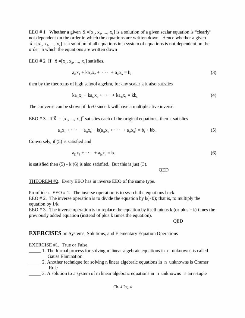
EEO # 1 Whether a given =[x1, x2, ..., xn] is a solution of a given scalar equation is “clearly”x

not dependent on the order in which the equations are written down. Hence whether a given=[x1, x2, ..., xn] is a solution of all equations in a system of equations is not dependent on the

xorder in which the equations are written down

EEO # 2 If =[x1, x2, ..., xn] satisfies. x

ai1x1 + kai2x2 + + ainxn = bi (3)

then by the theorems of high school algebra, for any scalar k it also satisfies

kai1x1 + kai2x2 + + kainxn = kbi. (4)

The converse can be shown if k0 since k will have a multiplicative inverse.

EEO # 3. If = [x1, ..., xn]T satisfies each of the original equations, then it satisfiesx

ai1x1 + + ainxn + k(aj1x1 + + ajnxn) = bi + kbj. (5)

Conversely, if (5) is satisfied and

aj1x1 + + ajnxn = bj (6)

is satisfied then (5) - k (6) is also satisfied. But this is just (3).QED

THEOREM #2. Every EEO has in inverse EEO of the same type.

Proof idea. EEO # 1. The inverse operation is to switch the equations back. EEO # 2. The inverse operation is to divide the equation by k(0); that is, to multiply theequation by 1/k.EEO # 3. The inverse operation is to replace the equation by itself minus k (or plus k) times thepreviously added equation (instead of plus k times the equation).

QED

EXERCISES on Systems, Solutions, and Elementary Equation Operations

EXERCISE #1. True or False._____ 1. The formal process for solving m linear algebraic equations in n unknowns is called Gauss Elimination_____ 2. Another technique for solving n linear algebraic equations in n unknowns is Cramer Rule _____ 3. A solution to a system of m linear algebraic equations in n unknowns is an n-tuple

Ch. 4 Pg. 4

(finite sequence) x 1, x 2, ..., x n in Kn (e.g., Rn or Cn ) such that all of the equations are true.

Ch. 4 Pg. 5

Handout #2 INTRODUCTION TO GAUSS ELIMINATION Professor Moseley

Gauss elimination can be used to solve a system of m linear algebraic equations over afield K in n unknown variables x 1, x 2, ..., x n in a finite number of steps.

a 11 x 1 + a 12 x 2 + + a 1n x n = b 1a 21 x 1 + a 22 x 2 + + a 2n x n = b 2 (1) a m1 x 1 + a m2 x 2 + + a mn x n = b m

Recall

DEFINITION #1. A solution of to (1) is an n-tuple x 1, x 2, ..., x n which may be considered as a (row) vector [ x 1, x 2, ..., x n ] (or column vector) in Kn (usually K is R or C ) such that all of theequations in (1) are true. The solution set for (1) is the set S = { [ x 1, x 2, ..., x n ] Kn: all of theequations in (1) are satisfied}. That is, the solution set is the set of all solutions. The set is theset where we look for solutions. In this case it is Kn. Two systems of linear algebraic equationsare equivalent if their solution set are the same (i.e., have the same elements).

Recall also the three elementary equation operations (EEO’s) that can be used on a set of linearequations which do not change the solution set.1. Exchange two equations2. Multiply an equation by a nonzero constant.3. Replace an equations by itself plus a scalar multiple of another equation.

Although other operations on the system of equations can be derived, if we restrictourselves to these operations, it is easier to develop computational algorithms that can be easilyprogramed on a computer.

DEFINITION #2. The coefficient matrix is the array of coefficients for the system (notincluding the right hand side, RHS).

(2)

11 12 1n

21 22 2n

m1 m21 mn

a a aa a a

a a a

Ch. 4 Pg. 6

DEFINITION #3. The augmented (coefficient) matrix is the coefficient matrix augmented bythe values from the right hand side (RHS).

x1 x2 xn+ ,*a 11 a 12 a 1n * b1 * Represents the first equation *a 21 a 22 a 2n * b2 * Represents the second equation* * * (3)* * ** * **a m1 a m2 a mn * bm * Represents the mth equation. -

Given the coefficient matrix A and the right hand side (“vector”) , we denote the associated b

augmented matrix as [A ]. (Note the slight abuse of notation since A actually includes theb

brackets. This should not cause confusion.)

ELEMENTARY ROW OPERATIONS. All of the information contained in the equations of alinear algebraic system is contained in the augmented matrix. Rather than operate on the originalequations using the elementary equation operations (EEO’s) listed above, we operate on theaugmented matrix using Elementary Row Operations (ERO's).

DEFINITION #4. We define the Elementary Row Operations (ERO's)1. Exchange two rows (avoid if possible since the determinant of the new coefficient matrix changes sign).2. Multiply a row by a non zero constant (avoid if possible since the determinant of the new coefficient matrix is a multiple of the old one).3. Replace a row by itself plus a scalar multiple of another row (the determinant of the new coefficient matrix is the same as the old one).

There is a clear one-to-one correspondence between systems of linear algebraic equations andaugmented matrices including a correspondence between EEO’s and ERO’s. We say that the twostructures are isomorphic. Using this correspondence and the theorems on EEO’s from theprevious handout, we immediately have the following theorems.

THEOREM #1. Suppose a system of linear equations is represented by an augmented matrixwhich we call the original augmented matrix (OAM) and that the OAM is operated on by an EROto obtain a new augmented matrix (NAM). Then the system of equations represented by the newaugmented matrix (NAM) has the same solution set as the system represented by the originalaugmented matrix (OAM).

THEOREM #2. Every ERO has an inverse ERO of the same type.

DEFINITION #5. If A and B are m×n (coefficient or augmented) matrices over the field F, wesay that B is row-equivalent to A if B can be obtained from A by finite sequence of ERO's.

Ch. 4 Pg. 7

THEOREM #3. Row-equivalence is an equivalence relation (Recall the definition ofequivalence relation given in the remedial notes or look up it up in a Modern Algebra text).

THEOREM #4 If A and B are m×n augmented matrices which are row-equivalent, then thesystems they represent are equivalent (i.e., have the same solution set).

Proof idea. Suppose A = A0 A1 Ak = B. Using induction and Theorem #1, the twosystems can be shown to have the same solution set.

DEFINITION #6. If A is a m×n (coefficient or augmented) matrices over the field F, we call thefirst nonzero entry in each row its leading entry. We say that A is in row-echelon form if: 1. All entries below a leading entry are zero,2. For i =2, ..., m, the leading entry in row i is to the right of the leading entry in row (i1),3. All rows containing only zeros are below any rows containing nonzero entries.If, in addition, 4. The leading entry in each row is one,5. All entries above a leading entry are zero,then A is in reduced-row-echelon form (or row-reduced-echelon form). If A is in row-echelon form (or reduced-row-echelon form) we refer to the leading entries aspivots.

For any matrix A, Gauss Elimination (GE) will always obtain a row-equivalent matrix U that is inrow-echelon form. Gauss-Jordan Elimination (GJE) will yield a row-equivalent matrix R that is in

reduced-row-echelon form. A b U c R d

GE GJE

EXAMPLE #1. To illustrate Gauss elimination we consider an example:

2x + y + z = 1 (1) 4x + y = -2 (2)2x + 2y + z = 7 (3)

It does not illustrate the procedure completely, but is a good starting point. The solution set Sfor (1), (2) and (3) is the set of all ordered triples, [x,y,z] which satisfy all three equations. Thatis,

S = { = [x, y, z] R3 : Equations (1), (2), and (3) are true }x

The coefficient and augmented matrices are

Ch. 4 Pg. 8

A = [A ] =

x y z2 1 14 1 02 2 1

b

x y z RHS

2 1 1 1 represents equation 14 1 0 2 represents equation 22 2 1 7 represents equation 3

Note that matrix multiplication is not necessary for the process of solving a system of linearalgebraic equations. However, you may be aware that we can use matrix multiplication to writethe system (1), (2), and (3) as A = where now it is mandatory that be a column vector

xb x

instead of a row vector. Also = [1, 2, 7]T is a column vector. (We use the transpose notationb

to save space and paper.)

GAUSS ELIMINATION. We now use the elementary row operations (ERO's) on the example ina systematic way known as (naive) Gauss (Jordan) Elimination to solve the system. Theprocess can be divided into three (3) steps.

Step 1. Forward Elimination (obtain zeros below the pivots).This step is also called the(forward) sweep phase.

R 2RR R

2 1 14 1 02 2 1

12

72 1

3 1

3 2

2 1 1 10 1 2 4

R 3R 0 3 2 8

2 1 10 1 2

0 4

1

4

0

4

This completes the forward elimination step. The pivots are the diagonal elements 2, -1, and -4. Note that in getting zeros below the pivot 2, we can do 2 ERO’s and only rewrite the matrixonce. The last augmented matrix represents the system.

2x + y + z = 1 We could now use 4z = 4 z = 1 y 2z = 4 back substitution y = 4 + 2z = 4 + 2(1) = 2 y = 2 4z = 4 . to obtain 2x = 1 y z = 1 (2) (1) = 2 x = 1.

The unique solution is sometimes written in the scalar form as x = 1, y = 2, and z = 1, but ismore correctly written in the vector form as the column vector [1,2,1]T. Instead of backsubstituting with the equations, we can use the following two additional steps using theaugmented matrix. When these steps are used, we refer to the process as Gauss-Jordanelimination.

Step 2. Gauss-Jordan Normalization (Obtain ones along the diagonal).

Ch. 4 Pg. 9

1/ 2 R

R1/ 4 R

2 1 10 -1 - 20 0 - 4

14

- 4

1

2

3

1 1/ 2 1/ 20 1 20 0 1

1/ 241

We could now use back substitution but instead we can proceed with the augmented matrix.

Step 3. Gauss-Jordan Completion Phase (Obtain zeros above the pivots) Variation #1 Right to Left.

1 3

2 3

nR 1/2nR 1 1/2 1/2 1/2R 2R 0 1 2 4

0 0 1 1

1 2nR 1/2nR 1 1/2 0 00 1 0 20 0 1 1

1 0 0 -10 1 0 20 0 1 1

x 1y 2z 1

Variation #2 (Left to Right)

1 2nR 1/ 2 R 1 1/2 1/2 1/2

0 1 2 40 0 1 1

1 3

2 3

nR 1/2nR 1 0 -1/2 3/2R 2R 0 1 2 4

0 0 1 1

1 0 00 1 00 0 1

-121

x 1y 2z 1

Note that both variations as well as back substitution result in the same solution, . Tx = [-1,2,1]

It should also be reasonably clear that this algorithm can be programmed on a computer. Itshould also be clear that the above procedure will give a unique solution for n equations in n unknowns in a finite number of steps provided zeros never appear on the diagonal. The casewhen zeros appear on the diagonal and we still have a unique solution is illustrated below. Themore general case of m equations in n unknowns where three possibilities exist is discussedlater.

EXAMPLE #2. To illustrate the case of zeros on the diagonal that are eliminated by rowexchanges consider:

y 2 z = 4 (4) 4 z = 4 (5)

2x + y + z = 1 (6)

The augmented matrix is

[A ] = b

x y z RHS

0 1 2 4 representsnequationn10 0 4 4 representsnequationn22 1 1 1 representsnequationn3

Note that there is a zero in the first row first column so that Gauss Elimination temporarily breaksdown. However, note that the augmented matrix is row equivalent to those in the previous

Ch. 4 Pg. 10

problem since it is just the matrix at the end of the forward step of that problem with the rows in adifferent order To establish a standard convention for fixing the breakdown, we go down the firstcolumn until we find a nonzero number. We then switch the first row with the first row with anonzero entry in the first column. (If all of the entries in the first column are zero, then x can beanything and is not really involved in the problem.) Switching Rows one and three we obtain

0 1 20 0 42 1 1

44

1

2 1 10 0 40 1 2

144

The 2 in the first row, first column is now our first pivot. We go to the second row, secondcolumn. Unfortunately, it is also a zero. But the third row, second column is not so we switchrows.

2 1 1 10 0 4 40 1 2 4

2 1 10 1 20 0 4

144

We now have the same augmented matrix as given at the end of the forward step for the previousproblem. Hence the solution is x = 1, y = 2, and z = 1. This can be written as the column vectorx = [1, 2, 1 ]T.

EXERCISES on Introduction to Gauss EliminationEXERCISE #1. True or False._____ 1. An elementary equation operation (EEO) that can be used on a set of linear algebraic equations which does not change the solution set is “Exchange two equations”._____ 2. An elementary equation operation (EEO) that can be used on a set of linear algebraic equations which does not change the solution set is “Multiply an equation by a nonzero constant”._____ 3. An elementary equation operation (EEO) that can be used on a set of linear algebraic equations which does not change the solution set is “Replace an equations by itself plus a scalar multiple of another equation”._____ 4. An elementary row operation (ERO) of type one that can be used on a matrix is “Exchange two rows”. _____ 5. An elementary row operation (ERO) of type two that can be used on a matrix is “Multiply a row by a nonzero constant”_____ 6. An elementary row operation (ERO) of type three that can be used on a matrix is “Replace a row by itself plus a scalar multiple of another row”._____ 7. There is a clear one-to-one correspondence between systems of linear algebraic equations and augmented matrices including a correspondence between EEO’s and ERO’s so that we say that the two structures are isomorphic. _____ 8. Every ERO has an inverse ERO of the same type.

Ch. 4 Pg. 11

_____ 9. If A and B are m×n (coefficient or augmented) matrices over the field K, we say that B is row-equivalent to A if B can be obtained from A by finite sequence of ERO's._____ 10. Row-equivalence is an equivalence relation _____ 11. If A and B are m×n augmented matrices which are row-equivalent, then the systems they represent are equivalent (i.e., have the same solution set)_____ 12. If A is a m×n (coefficient or augmented) matrix over the field K, we call the first nonzero entry in each row its leading entry.

EXERCISE #2. Solve 4x + y = -2 2x + 2y + z = 7

2x + y + z = 1

EXERCISE #3. Solve x1 + x2 + x3 + x4 = 1 x1 + 2x2 + x3 = 0 x3 + x4 = 1 x2 + 2x3 + x4 = 1

EXERCISE #4. Solve 4x + y = -2 2x + y + z = 7

2x + y + z = 1

EXERCISE #5. Solve x1 + x2 + x3 + x4 = 1 x1 + 2x2 + x3 = 0 x3 + x4 = 1 x2 + 2x3 + 2x4 = 3

EXERCISE #6. Solve 4x + y = -2 2x + 2y + z = 5

2x + y + z = 1

EXERCISE #7. Solve 4x + y = -2 2x + 2y + z = 1

2x + y + z = 1

Ch. 4 Pg. 12

Handout #3 CONNECTION WITH MATRIX Professor MoseleyALGEBRA AND ABSTRACT LINEAR ALGEBRA

By using the definition of matrix equality we can think of the system of scalar equations

a 11 x 1 + a 12 x 2 + + a 1n x n = b 1a 21 x 1 + a 22 x 2 + + a 2n x n = b 2 (1) a m1 x 1 + a m2 x 2 + + a mn x n = b m

as one “vector” equation where “vector” means an n-tuple or column vector. By using matrixmultiplication (1) can be written as

(2)mxn nx1 mx1A x b

where

= [xi] Kn, = [bi]Km, A = = [aij]Kmxn .x

xx

x

1

2

n

b

bb

b

1

2

m

a a aa a a

a a a

11 12 1n

21 22 2n

m1 m21 mn

If we think of Kn and Km as vector spaces, we can define

T( ) = (3)x A x

mxn nx1

so that T is a mapping from Kn to Km. We write T: Kn Km. A mapping from a vector spaceto another vector space is called an operator. We may now view the system of scalar equationsas the operator equation:

T( ) = (4)xb

A column vector Kn is a solution to (4) if and only if it is a solution to (1) or (2). Solutionsx

to (4) are just those vectors in Kn that get mapped to in Km by the operator T. Thex

b

equation T( ) = (5)x

0

is called homogeneous and is the complementary equation to (4). Note that it always has

Ch. 4 Pg. 13

= = [0, 0, ... , 0]T Kn as a solution. = is called the trivial solution to (5) since it is x

0 x

0

always a solution. The question is “Are there other solutions?” and if so “How many?”. We now have a connection between solving linear algebraic equations, matrix algebra, and abstract linear algebra. Also we now think of solving linear algebraic equations as an example of amapping problem where the operator T:Rn Rm is defined by (3) above. We wish to find all solutions to the mapping problem (4). To introduce this topic, we define what we mean by a linear operator from one vector space to another.

DEFINITION #1. An operator T:V W is said to be linear if , V and scalars α,β, x y

it is true that T( α + β ) = α T( ) + β T( ). (6)x y x y

T: Kn Km defined by T( ) = is one example of a linear operator. We will give others x A x

mxn nx1

later. To connect the mapping problem to matrix algebra we reveal that if m = n, then (1) (2) and (4) have a unique solution if and only if the matrix A is invertible.

THEOREM #1. Suppose m = n so that (1) has the same number of equations as unknowns. Then (1), (2), and (4) have a unique solution if and only if the matrix A is invertible.

EXERCISES on Connection with Matrix Algebra and Abstract Linear Algebra

EXERCISE #1. True or False._____ 1. Since Kn and Km are vector spaces, we can define T( ) = so that T is a

x A xmxn nx1

mapping from Kn to Km. _____ 2. A mapping from a vector space to another vector space is called an operator. _____ 3. Solutions to are just those vectors in Kn that get mapped to in Km

mxn nx1 mx1A x b

x

b

by the operator T( ) = . x A x

mxn nx1

_____ 4. The equation T( ) = is called homogeneous and is the complementary equation to x

0

where T( ) = . mxn nx1 mx1T x b

x A x

mxn nx1

_____ 5. = is called the trivial solution to the complementary equation to .x

0

mxn nx1 mx1A x b

_____ 6. An operator T:V W is said to be linear if , V and scalars α,β, it is truex y

that T( α + β ) = α T( ) + β T( ).x y x y_____ 7. The operator T: Kn to Km defined by T( ) = is a linear operator.

x A xmxn nx1

_____ 8. has a unique solution if and only if the matrix A is invertible.nxn nx1 nx1A x b

Ch. 4 Pg. 14

Handout #4 POSSIBILITIES FOR Professor MoseleyLINEAR ALGEBRAIC EQUATIONS

We consider the three possible outcomes of applying Gauss elimination to the system ofscalar algebraic equations:

a 11 x 1 + a 12 x 2 + + a 1n x n = b 1a 21 x 1 + a 22 x 2 + + a 2n x n = b 2 (1) a m1 x 1 + a m2 x 2 + + a mn x n = b m

THEOREM. There exists three possibilities for the system (1):1. There is no solution.2. There exists exactly one solution.3. There exists an infinite number of solutions

We have illustrated the case where there exists exactly one solution. We now illustrate the caseswhere there exists no solution and an infinite number of solutions.

EXAMPLE. Solve

E1 x + y + z = b1E2 2x + 2y + 3z = b2 (2)E3 4x + 4y + 8z = b3

if has the values 1) and 2) .b

bbb

1

2

3

b b

111

1

b b

110

2

Solution: Forward Step. Reduce the augmented matrix

R 2R

R 4R

1 1 1

2 2 3

4 4 8

b

b

b2 1

3 1

1

2

3

R 4R

1 1 10 0 10 0 4

bb 2bb 4b3 2

1

2 1

3 1

1 1 10 0 10 0 0

bb b

b 4b + 4b

1

2 1

3 2 1

as R3 4R2 b3 4b1 4(b2 2b1) = b3 4b2+4b1

This completes the forward elimination step. We see that (2) has a solution if and only ifb3 4b2 + 4b1 = 0 or 4b1 4b2 + b3 = 0. This means that the range of the operator T associatedwith the matrix A is the plane in R3 through the origin whose equation in x,y,z variables is

Ch. 4 Pg. 15

P: 4x 4y +z = 0 where P R3. If = [1,1,1]T then 4(1) 4(1) + 1 = 1 0 and hence we b b1

have no solution. If = [1,1,0]T then 4(1) 4(1) + 0 = 0 so there exists a solution. In fact b b 2

there exists an infinite number of solutions. The pivots are already ones. We finish the Gauss-Jordan process for = [1,1,0]T . Our augmented matrix is

b b 2

1 2R R 1 1 1 1

0 0 1 10 0 0 0

1 1 0 20 0 1 10 0 0 0

x y 2 z 1 0 0

x 2 - yz 1

We can now write a (parametric) formula for the infinite number of solutions.

= = + y x

xyz

2 yy1

201

110

It will become clear why one wishes to writw the solution in this form after you learn to solvedifferential equations.

CONVENIENT CHECKS. There are convenient checks for the vectors that appear in theformula for the infinite number of solutions. Satisfying these checks does not guarantee a correctsolution. However, failing these checks does guarantee an error.

Since we claim to have all solutions to , letting y = 0, we see that 3x3 3x1 3x1A x b

= [2, 0, 1]T should be a (particular) solution to . (There are an infinite number ofpx Ax b

solutions.) u + v + w = 1 2 + 0 1 = 1 2u + 2v + 5w = 1 2(2) + 2(0) + 5(1) = 14u + 4v + 5w = 0 4(2) + 4(0) + 8(1) = 0

Hence this part of the formula for the solution checks. Careful analysis indicates that = [1, 1, 0]T should be a solution to the complementary (homogeneous) equation .

x1 Ax 0

u + v + w = 0 1 + 1 + 0 = 0 2u + 2v + 5w = 0 2( 1) +2(1) + 5(0) = 0 4u + 4v + 8w = 0 4( 1) +4(1) + 8(0) = 0

Hence this part of the formula for the solution also checks.

EXERCISES on Possibilities for Linear Algebraic Equations

EXERCISE #1. True or False._____ 1. There exists three possibilities for the system .

mxn nx1 mx1A x b

_____ 2. One possibility for the system is that there is no solution.mxn nx1 mx1A x b

Ch. 4 Pg. 16

_____ 3. One possibility for the system is that there exists exactly one solution.mxn nx1 mx1A x b

_____ 4. One possibility for the system is an infinite number of solutions.mxn nx1 mx1A x b

EXERCISE #2. Solve x + y + z = b1 2x + 2y + 3z = b2 4x + 4y + 8z = b3

if has the values 1) and 2) .1

2

3

bb b

b

1

1b b 1

2

2

1b b 2

0

EXERCISE #3. Solve x + y + z = b1 2x + 2y + 3z = b2 4x + 4y + 4z = b3

if has the values 1) and 2) .1

2

3

bb b

b

1

1b b 2

4

2

1b b 1

2

Ch. 4 Pg. 17

Handout #2 WRITING SOLUTIONS OF Professor MoseleyLINEAR ALGEBRAIC EQUATIONS

Consider the system of linear equations

(1)A x bmxn nx1 mx1

Suppose we apply Gauss-Jordan elimination so that

GE GJE

mxn mxnmxnmx1 mx1 mx1A b U c R d

where U is an upper triangular matrix obtained using Gauss Elimination, is the result of applyingc

these same operations to , R is the row- reduced-echelon form of A obtained using Gauss -b

Jordan elimination, and is the result of applying these same operations to . This meansd

b

that the matrix has zeros above as well as below the pivots. Recall that there all threeR dmxn mx1

cases: 1) No solution, 2) Exactly one solution (a unique solution), and 3) An infinite number ofsolutions.

1) If there is a row in where the entries in R are all zero and the entry in is nonzero R dmxn mx1

d

(this corresponds to an equation of the form 0 = di 0). Since this is not true, the system has no solution, and you conclude by writing: No Solution.

2) If there are m n rows of all zeros (including the elements in ) and so n pivots (dependentd

variables) then each variable in is determined uniquely and there is exactly one solution. x

Conclude by giving the solution explicitly in both scalar and vector form.3) If there are an infinite number of solutions we proceed as follows:

a) Separate the variables (i.e. the columns) into two groups. Those corresponding to pivots are the dependent (basic) variables. Those not corresponding to pivots are the independent (free) variables.b) Write the equations that correspond to the augmented matrix [R ].

d

c) Solve these equations for the dependent variables in terms of the independent variables. (This is easy if GJE is used).d) Replace the dependent variables in the vector x = [x1, , xn]T to obtain x in terms of the independent variables only.

e) Write the infinite number of solutions in the paramentric form x

x x c xp i ii 1

k

Ch. 4 Pg. 18

x = 1 y = 2 Scalar formz = 1

where the ci’s are the independent variables. Thus we see that there is a solution for each set of paramenter values.

Alternately we see that x p can be obtained by letting all the ci’s (i.e. the independent variables) be zero. If then can be taken to be . The above procedure will in fact make it

b 0

x p

0

zero.) Hence the vectors xI can be obtained by letting and letting each independent b 0

variable be one with the rest of the independent variables equal to zero.

EXAMPLE#1 . Recall that the solution process for

2x + y + z = 1 (1) 4x + y = 2 (2)2x + 2y + z = 7 (3)

using Gauss-Jordan elimination (right to left) on augmented matrices is

2 1

3 1

2 1 1 1R 2R 4 1 0 2R R 2 2 1 7

R R

2 1 10 1 2

3 2

1

83 2

3 0

4

1 / 2 RR

1 / 4 R

2 1 10 1 20 0 4

144

1

2

3

R 1/ 2 RR 2R

1 1/ 2 1/ 20 1 20 0 1

1/ 241

1 3

2 3

R 1/ 2 R 1 1/ 2 00 1 00 0 1

021

1 2

1 0 00 1 00 0 1

-121

Vector form.x

121

EXAMPLE#2 . Recall that the solution process for

E1 x + y + z = b1E2 2x + 2y + 3z = b2 (2)E3 4x + 4y + 8z = b3

if = [1,1,1]T using Gauss elimination (only the forward sweep is needed) on augmented b b1

Ch. 4 Pg. 19

matrices is

R 2RR 4R

1 1 12 2 34 4 8

111

2 1

3 1

R 4R

1 1 10 0 10 0 4

1-1-33 2

1 1 10 0 10 0 0

1-11

x y z 1z 10 1

The last equation (0=1) is not true so we see that the equations are inconsistent and that there isno solution. We write NO SOLUTION.

On the other hand, if = [1,1,0]T using Gauss-Jordan elimination on augmented matrices is b b1

R 2RR 4R

1 1 12 2 34 4 8

110

2 1

3 1

3 2

1 1 1 10 0 1 1

R 4R 0 0 4 3

1 2R R 1 1 1 10 0 1 10 0 0 0

1 2R R 1 1 0 20 0 1 10 0 0 0

x y 2 z 1 0 0

x 2 - yz 1

We can now write a (parametric) formula for the infinite number of solutions.

= = + y Vector Form Scalar Formx 2 - yz 1

2 yy1

20-1

110

x 1 y(y y)z 1

Ch. 4 Pg. 20

EXERCISES on Writing Solutions of Linear Algebraic Equations

EXERCISE #1. Suppose the Gauss process yields x + y + z = b1 2y + 3z = b2 8z = b3If = [1,1,1]T , give the solution and the solution set. What is the difference inT

1 2 3 1b =[b ,b ,b ] = b

these two questions. How many solutions are there? The solution should be written as ______. If = [0,0,0]T , give the solution and the solution set. What is the difference inT

1 2 3 1b =[b ,b ,b ] = b

these two questions. How many solutions are there? The solution should be written as ______.

EXERCISE #2. Suppose the Gauss-Jordan process yields 1 2

2 1

3 2 1

b -b1 0 00 1 0 b -b0 0 0 b -b -b

If = [1,1,1]T , give the solution and the solution set. What is the difference inT1 2 3 1b =[b ,b ,b ] = b

these two questions. How many solutions are there? The solution should be written as ______. If = [1,1,0]T , give the solution and the solution set. What is the difference inT

1 2 3 1b =[b ,b ,b ] = b

these two questions. How many solutions are there? The solution should be written as _____.

Ch. 4 Pg. 21

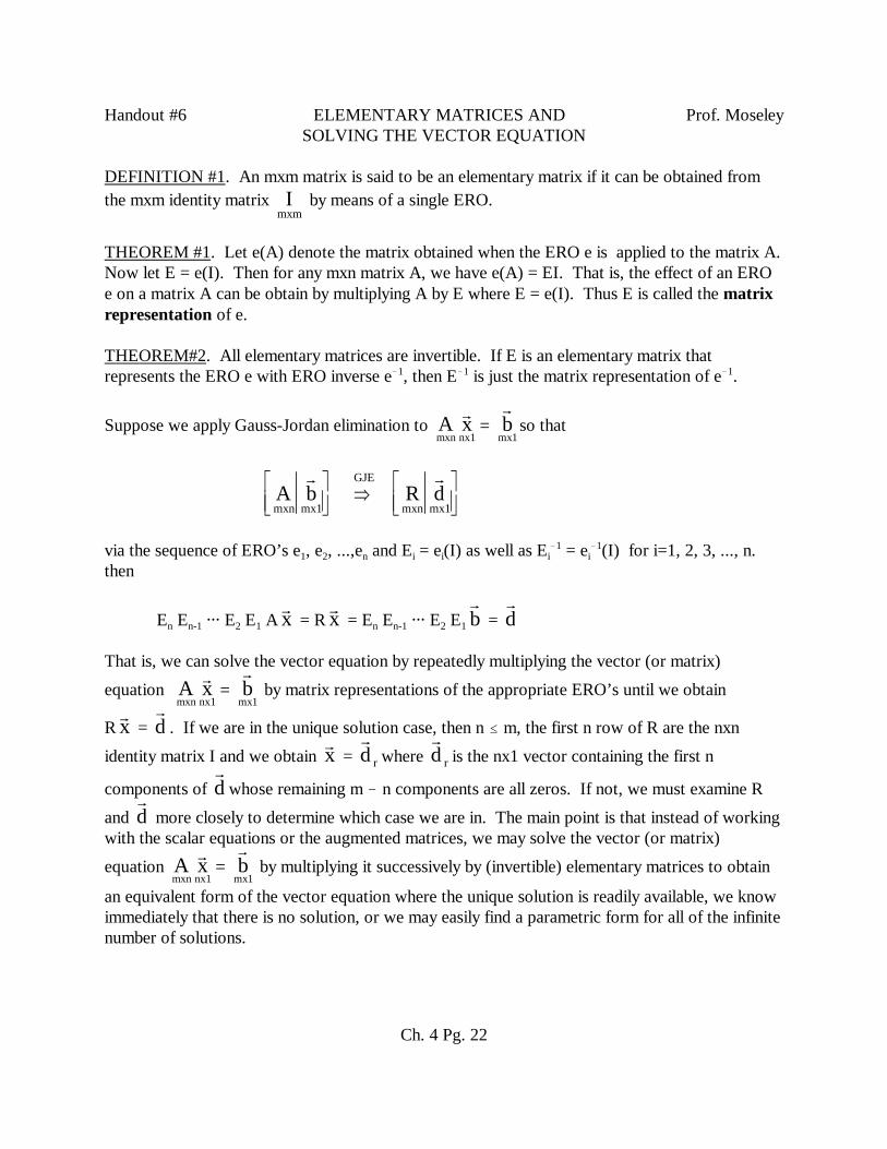
Handout #6 ELEMENTARY MATRICES AND Prof. MoseleySOLVING THE VECTOR EQUATION

DEFINITION #1. An mxm matrix is said to be an elementary matrix if it can be obtained fromthe mxm identity matrix by means of a single ERO.I

mxm

THEOREM #1. Let e(A) denote the matrix obtained when the ERO e is applied to the matrix A. Now let E = e(I). Then for any mxn matrix A, we have e(A) = EI. That is, the effect of an EROe on a matrix A can be obtain by multiplying A by E where E = e(I). Thus E is called the matrixrepresentation of e.

THEOREM#2. All elementary matrices are invertible. If E is an elementary matrix thatrepresents the ERO e with ERO inverse e1, then E1 is just the matrix representation of e1.

Suppose we apply Gauss-Jordan elimination to so that A x bmxn nx1 mx1

A b R dmxn mx1

GJE

mxn mx1

via the sequence of ERO’s e1, e2, ...,en and Ei = ei(I) as well as Ei1 = ei

1(I) for i=1, 2, 3, ..., n.then

En En-1 E2 E1 A = R = En En-1 E2 E1 = x x

b

d

That is, we can solve the vector equation by repeatedly multiplying the vector (or matrix)equation by matrix representations of the appropriate ERO’s until we obtain A x b

mxn nx1 mx1

R = . If we are in the unique solution case, then n m, the first n row of R are the nxnx

d

identity matrix I and we obtain = where is the nx1 vector containing the first nx

d r

d r

components of whose remaining m n components are all zeros. If not, we must examine Rd

and more closely to determine which case we are in. The main point is that instead of workingd

with the scalar equations or the augmented matrices, we may solve the vector (or matrix)equation by multiplying it successively by (invertible) elementary matrices to obtainA x b

mxn nx1 mx1

an equivalent form of the vector equation where the unique solution is readily available, we knowimmediately that there is no solution, or we may easily find a parametric form for all of the infinitenumber of solutions.

Ch. 4 Pg. 22

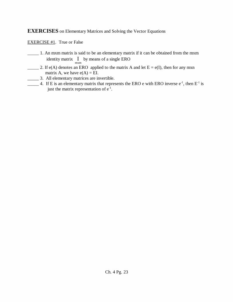
EXERCISES on Elementary Matrices and Solving the Vector Equations

EXERCISE #1. True or False

_____ 1. An mxm matrix is said to be an elementary matrix if it can be obtained from the mxm identity matrix by means of a single EROI

mxm_____ 2. If e(A) denotes an ERO applied to the matrix A and let E = e(I), then for any mxn matrix A, we have e(A) = EI. _____ 3. All elementary matrices are invertible. _____ 4. If E is an elementary matrix that represents the ERO e with ERO inverse e-1, then E-1 is just the matrix representation of e-1.

Ch. 4 Pg. 23

A SERIES OF CLASS NOTES TO INTRODUCE LINEAR AND NONLINEAR PROBLEMS TO ENGINEERS, SCIENTISTS, AND APPLIED MATHEMATICIANS

LINEAR CLASS NOTES:A COLLECTION OF HANDOUTS FOR

REVIEW AND PREVIEW OF LINEAR THEORY

INCLUDING FUNDAMENTALS OF LINEAR ALGEBRA

CHAPTER 5

Linear Operators,

Span, Linear Independence,

Basis Sets, and Dimension

1. Linear Operators

2. Spanning Sets

3. Linear Independence of Column Vectors

4. Basis Sets and Dimension

Ch. 5 Pg. 1

Handout #1 LINEAR OPERATOR THEORY Professor Moseley

In this handout, we preview linear operator theory. The most important examples oflinear operators are differential and integral operators and operators defined by matrixmultiplication. These arise in many applications. Lumped parameter systems (e.g., linearcircuits and mass spring systems) give rise to discrete operators defined on finite dimensionalvector spaces (e.g., Rn). Differential and integral equations (e.g., Maxwell’s equations and theNavier-Stokes equation) are used to model distributed (continuum) systems and require infinitedimensional vector spaces. These give rise to differential and integral operators on functionspaces.

Even without covering any topics in differential equations, your background in calculus should be sufficient to see how discrete and continuous operators are connected as linearoperators on a vector space.

A function or map T from one vector space V to another vector space W is often call anoperator. If we wish to think geometrically (e.g., if V and W are R2 or R3) rather thanalgebraically we might call T a transformation.

DEFINITION 1. Let V and W be vector spaces over the same field K. An operator T:V W issaid to be linear if , V and scalars α,βK, it is true that

x y

T( α + β ) = α T( ) + β T( ). (1)x y x y

THEOREM 1. Let V and W be vector spaces over the same field K. An operator T: V W islinear if and only if the following two properties hold: i) , ε V implies T( + ) = T( ) + T( ) (2)

x y x y x y ii) αK and ε V implies T(α ) = α T( ). (3)

x x x

EXAMPLE 1 Let the operator T:Rn Rm be defined by matrix multiplication of the column vector by the m× n matrix A; that is, let

x

T( ) =df (4)x

mxn nx1A x

where Rn and Rm×n. Then T is a linear

1

2

mxn

n

xx

x

x

11 12 1n

21 22 2n

mxn

m1 m21 mn

a a aa a a

a a a

A

operator.

Ch. 5 Pg. 2

EXAMPLE 2 Let I = (a,b). The operator D:C1(I,R) C(I,R) defined by

D(f) =df (5)dfdx

where f ε C1(I,R) = {f:I R: exists and is continuous on I} anddfdx

C(I, R) ={f:I R:f is continuous on I}. Then D is a linear operator. We may restrict D to A (I, R) ={f:I R:f is analytic on I} so that D:A (I, R) A (I, R) maps a vector space back toitself.

DEFINITION #2. Let T:VW be a mapping from a set V to a set W. The set R(T) = {y W: there exists an xV such that y = T(x) } is called the range of T. If W has an additive structure (i.e., a binary operation which we call addition) with an additive identity which we call 0, then the set N(T) = {xV: T(x) = 0} is called the null set of T (or nullity of T).

If T is a linear operator from a vector space V to another vector space W, we can say more.

THEOREM #2 Let T:VW be a linear operator from a vector space V to a vector space W. The range of T, R(T) = { W: there exists an V such that = T( ) }, is a subspace of W

y x y xand the null set of T, N(T) = { V: T( ) = 0} is a subspace of V.

x x

We rename these sets.

DEFINITION #3. Let T:VW be a linear operator from a vector space V to another vectorspace W. The set R(T) = { W: there exists an V such that = T( ) } is called the

y x y xrange space of T and the set N(T) = { V: T( ) = } is called the null space of T. .

x x0

Ch. 5 Pg. 3

EXERCISES on Linear Operator Theory

EXERCISE #1. True or False._____ 1. A linear circuit is an example of a lumped parameter system.

_____ 2. Amass/spring system is an example of a lumped parameter system.

_____ 3. A function or map T from one vector space V to another vector space W is often call an operator. _____ 4. An operator T:V W is said to be linear if , V and scalars α,βK, it is true

x y that T( α + β ) = α T( ) + β T( ).

x y x y_____ 5. An operator T: V W is linear if and only if the following two properties hold: i) , ε V implies T( + ) = T( ) + T( ) and ii) αK and ε V implies

x y x y x y x

T(α ) = α T( ).x x

_____ 6. The operator T:Rn Rm defined by is a linear operator.mxn nx1

T(x) A x

_____ 7. The operator D:C1(a,b) C(a,b) be defined by D(f) =df is a linear operator.dfdx

_____ 8. C(a,b) ={f:(ab) R:f is continuous}.

_____ 9. C1(a,b) = {f:(a,b) R: exists and is continuous}. dfdx

_____ 10. If T:VW , then the set R(T) = {y W: there exists an xV such that y = T(x) } is called the range of T. _____ 11. If T:VW and W has an additive structure (i.e., a binary operation which we call addition) with an additive identity which we call 0, then the set N(T) = {xV: T(x) = 0} is called the null set of T (or nullity of T)._____ 12. If T:VW is a linear operator from a vector space V to a vector space W, then the range of T, R(T) = { W: there exists an V such that = T( ) }, is a

y x y x subspace of W_____ 14.If T:VW is a linear operator from a vector space V to a vector space W, then the null set of T, N(T) = { V: T( ) = 0} is a subspace of V.

x x_____ 15. If T:VW is a linear operator from a vector space V to another vector space W, then the set R(T) = { W: there exists an V such that = T( ) } is called the

y x y x range space of T. _____ 16. If T:VW is a linear operator from a vector space V to another vector space W, then the set N(T) = { V: T( ) = } is called the null space of T.

x x0

Ch. 5 Pg. 4

Handout # 2 SPANNING SETS Professor Moseley

DEFINITION #1. If , , , are vectors in a vector space V and α1,α2,,αn x1

x2x n

are scalars, then

α, + α2 + + αn = x1

x2x n

n

i 1i 1

x

is called a linear combination of the vectors. (It is important to note that a linear combinationallows only a finite number of vectors.)

EXAMPLE #1. Consider the system of linear algebraic equations:

2x + y + z = 14x + y = -3 x - 2y - z = 0 .

This set of scalar equations can be written as the vector equation

x + y + z = 241

112

101

13

0

where the left hand side (LHS) is a linear combination of the (column vectors whose components come from the) columns of the coefficient matrix

A = .

2 1 14 1 01 2 1

If we generalize Example #1, we obtain:

THEOREM #1. The general system

(1)A x bnxn nx1 nx1

has a solution if and only if the vector can be written as a linear combination of theb

Ch. 5 Pg. 5

columns of A. That is, is in the range space of T( ) = A if and only if can be written asb x x

b

a linear combination of the (column vectors whose components come from the) columns of thecoefficient matrix. A.

DEFINITION #2. Let S be a (finite) subset of a subspace W of a vector space V. If everyvector in W can be written as a linear combination of (a finite number of) vectors in S, then S is said to span W or to form a spanning set for W. On the other hand, if S is any (finite) set ofvectors, the span of S, written Span(S), is the set of all possible linear combinations of (a finitenumber of) vectors in S.

THEOREM #2. For any (finite) subset S of a vector space V, Span (S) is a subspace of V.

THEOREM #3. If (a finite set) S is a spanning set for W, then Span S = W.

EXAMPLES. Consider the following subsets of R3.

1. S = {[1,0,0]T} = {i}. Then Span (S) = {x i: x R} = x - axis. 2. S = {[1,0,0]T, [0,1,0]T} = {i, j}. Then Span (S) = {x i+y j: x, y R} = the xy plane. 3. S = {[1,0,0]T, [1,1,0]T} = {i, i+j}. Then Span (S) = xy plane. 4. S = {[1,0,0]T, [0,1,0]T, [1,1,0]T} = {i, j, i+j}. Then Span (S) = xy plane.

DEFINITION #3. For any matrix , the span of the set of column vectors is the columnAmxn

space of A. The usual notation for the column space is R(A) and sometimes RA. Normally wewill use R(A). The reason for this notation is that when we think of the operator T( ) defined

xby (matrix) multiplication of the matrix by the column vector = [x1,,xn]T, we see that T A

mxn

x

maps vectors Rn into vectors = A Rm, the column space R(A) is seen to be thex y

xrange (space) of T.

COMMENT. Consider the general system (1) above. Theorem #1 can now be rephrased to say that (1) has a solution if and only if is in the column space of A (i.e. in the range of the

b

operator T).

DEFINITION 4. For any matrix , the span of the set of row vectors is the row space Amxn

of A. The usual notation for the row space is R(AT) and sometimes RAT since the row space of A is the column space of AT. Normally we will use R(AT).

If we think of the operator TT( ) defined by (matrix) multiplication of the matrix by the x A

mxn

T

column vector = [y1,,ym]T, we see that AT maps vectors Rm into vectors = AT Rn, y y x y

Ch. 5 Pg. 6

the row space R(AT) is seen to be the range (space) of AT.

Recall that all of the coefficient matrices for the associated linear systems of algebraic equations obtained in the process of doing Gauss elimination are row equivalent. Hence they all have the same row space. However, they do not have the same column space.

EXERCISES on Spanning Sets

EXERCISE #1. True or False._____ 1. If , , , are vectors in a vector space V and α1,α2,,αn are scalars, then

x1x2

x n

α, + α2 + + αn = is a linear combination of the vectorsx1

x2x n

n

i 1i 1

x

_____ 2. A linear combination allows only a finite number of vectors.

_____ 3. The linear algebraic equations: 2x + y + z = 1, 4x + y = 3, x 2y z = 0, is a system of scalar equations._____ 4. The coefficient matrix for the system of linear algebraic equations: 2x + y + z = 1,

4x + y = 3, x 2y z = 0 is A = .

2 1 14 1 01 2 1

_____ 5. The linear algebraic equations: 2x + y + z = 1, 4x + y = 3, x 2y z = 0 can be

written as the vector equation x + y + z = .241

112

101

13

0

_____ 5. The left hand side (LHS) of the vector equation x + y + z 241

112

101

= is a linear combination of the column vectors whose components come from 13

0

the columns of the coefficient matrix A = .

2 1 14 1 01 2 1

_____ 6. The general system has a solution if and only if the vector can be writtenA x bnxn nx1 nx1

b

Ch. 5 Pg. 7

as a linear combination of the columns of A. _____ 7. is in the range space of T( ) = A if and only if can be written as a linear

b x x

b

combination of the column vectors whose components come from the columns of the coefficient matrix A._____ 8. If S be a finite subset of a subspace W of a vector space V and every vector in W can be written as a linear combination of a finite number of vectors in S, then S is said to span W or to form a spanning set for W._____ 9. If S be a finite subset of a subspace W of a vector space V, then the span of S, written Span(S), is the set of all possible linear combinations of a finite number of vectors in S._____ 10. For any finite subset S of a vector space V, Span (S) is a subspace of V.

_____ 11. If S be a finite subset of a subspace W of a vector space V and S is a spanning set for W, then Span S = W._____ 12. For any matrix , the span of the set of column vectors is the column space of A.A

mxn

_____ 13. The usual notation for the column space is R(A) and sometimes RA.

_____ 14. The reason that R(A) is the column space of A is that when we think of the operator

T( ) defined by matrix multiplication of the matrix by the column vector x A

mxn

= [x1,,xn]T, we see that T maps vectors Rn into vectors = A Rm x x y

x which is the column space R(A)_____ 14. The column space R(A) is the range space of T.

_____ 15. has a solution if and only if is in the range of the operator T( ) = A .A x bnxn nx1 nx1

b

x x

_____ 16. has a solution if and only if is in the column space of A. A x bnxn nx1 nx1

b

_____ 17. For any matrix , the span of the set of row vectors is the row space of A. Amxn

_____ 18. The usual notation for the row space is R(AT) and sometimes RAT since the row space of A is the column space of AT. _____ 19. If we think of the operator TT( ) defined by (matrix) multiplication of the matrix

x by the column vector = [y1,,ym]T, we see that AT maps vectors Rm into A

mxn

T y y

vectors = AT Rn, the row space R(AT) is seen to be the range space of AT.x y

Ch. 5 Pg. 8

Handout #3 LINEAR INDEPENDENCE (OF COLUMN VECTORS) Professor Moseley

DEFINITION #1. Let V be a vector space. A finite set of vectors V isS {x ,..., x }1 k

linearly independent (.i.) if the only set of scalars c1, c2, ..., ck which satisfy the (homogeneous)vector equation

(1)1 1 2 2 k kc x c x c x 0

is c1 = c2 = = cn = 0; that is, (1) has only the trivial solution. If there is a set of scalars not allzero satisfying (1) then S is linearly dependent (.d.).

It is common practice to describe the vectors (rather than the set of vectors) as beinglinearly independent or linearly dependent. Although this is technically incorrect, it is widespread, and hence we accept this terminology. Since we may consider (1) as a linearhomogeneous equation with unknown vector [ c1, c2, ..., cn] Rn, if (1) has one nontrivialsolution, then it in fact has an infinite number of nontrivial solutions. As part of the standardprocedure for showing that a set is linearly dependent directly using the definition (DUD) youmust exhibit one (and only one) such non trivial solution. To show that a set is linearlyindependent directly using the definition (DUD) you must show that the only solution of (1) isthe trivial solution (i.e. that all the ci's must be zero). Before looking at the application of thisdefinition to column vectors, we state four theorems.

THEOREM #1. Let V be a vector space. If a finite set of vectors V containsS {x ,..., x }1 k

the zero vector, then S is linearly dependent.

THEOREM #2. Let V be a vector space. If , then V is linearly independent. x 0 S {x}

Proof. To show S is linearly independent we must show that c1 implies that c1 = 0. But x = 0

by the zero product theorem, if c1 is true then c1 = 0 or . But by hypothesis . x = 0

x = 0 x 0

Hence c1 implies c1 = 0. Hence S = where is linearly independent. x = 0 {x} x 0

Q.E.D.

THEOREM #3. Let V be a vector space and S = { , } V. If either or is the zeroxy x

yvector, then S is linearly dependent.

THEOREM #4. Let V be a vector space and S = { , } V where and are nonzeroxy x

yvectors. Then S is linearly dependent if and only if one vector is a scalar multiple of the other.

Although the definition is stated for an abstract vector space and hence applies to any

Ch. 5 Pg. 9

vector space and we have stated some theorems in this abstract setting, in this section we focus oncolumn vectors in Rn (or Cn or Kn). Since we now know how to solve a system of linearalgebraic equations, using this procedure, we can develop a “procedure” to show that a finite setin Rn (or Cn or Kn) is linearly independent. We also show how to give sufficient conditions toshow that a finite set in Rn (or Cn or Kn) is linearly dependent.

PROCEDURE. To determine if a set V is linearly independent or linearlyS {x ,..., x }1 k

dependent, we first write down the equation (1) and try to solve. If we can show that the onlysolution is the trivial solution c1 = c2 = = cn = 0, then we have shown directly using thedefinition (DUD) of linear independence that S is linearly independent. On the other hand(OTOH), if we can exhibit a nontrivial solution, then we have shown directly using thedefinition of linear dependence that S is linearly dependent. We might recall that the lineartheory assures us that if there is one nontrivial solution, that there are an infinite number ofnontrivial solutions. However, to show that S is linearly dependent directly using the definition,it is not necessary (or desirable) to find all of the nontrivial solutions. Although you could arguethat once you are convinced (using some theorem) that there are an infinite number of solutions,then we do not need to exhibit one, this will not be considered to be a proof directly using thedefinition (as it requires a theorem). Thus to prove that S is linearly dependent directly using thedefinition of linear dependence, you must exhibit one nontrivial solution. This will help you tobetter understand the concepts of linear independence and linear dependence. We apply these“procedures” to finite sets in Rn (or Cn). For Rn (or Cn) (1) becomes a system ofS {x ,..., x }1 k

n equations (since we are in Rn (or Cn) ) in k unknowns (since we have k vectors). (This can beconfusing when applying general theorems about m equations in n unknowns. However, thisshould not be a problem when using DUD on specific problems.)

EXAMPLE #1. Determine (using DUD) if is linearly independent.1 2 1

S , ,1 3 2

Solution. (This is not a yes-no question and a proof is required). Assume

(2)1 2 3

1 2 1 0c c c

1 3 2 0

and (try to) solve. The vector equation (2) is equivalent to the two scalar equations (since we arein R2) in three unknowns (since S has three vectors).

c1+ 2c2 + c3 = 0 c1+ 3c2 + 2c3 = 0 (3)

Simple systems can often be solved using ad hoc (for this case only) procedures. But for

Ch. 5 Pg. 10

complicated systems we might wish to write this system in the form and use GaussAc 0

elimination (on a computer). Note that when we reduce A we do not have to augment. Why?

For this example and . Since the system is homogeneous we can1 2 1

A1 3 2

1

2

3

cc c

c

solve by reducing A without augmenting (Why?).

1 2 3 1 2 3 3 3 3

2 3 2 31 2

c 2c c 0 c 2c c 2c c c1 2 1 1 2 1c c 0 c cR R 1 3 2 0 1 1

Hence the general solution of (2) is .1 3

2 3 3

3 3

c c 1c c c 1c c 1

Hence there are an infinite number of solutions. They are the vectors in the subspace W = { R3 : = c [2, -1, 1]T with c R}. Since there is a nontrivial solution, S is linearly

x xdependent. However, we must exhibit one nontrivial solution which we do by choosing c1=1, c2 = 1, and c3 = 1. Hence we have

(4)1 2 1 0

(1) ( 1) (1)1 3 2 0

Since we have exhibited a nontrivial linear combination of the vectors in S, (4) alone proves that S is a linearly dependent set in the vector space R2 QED

It may be easy to guess a nontrivial solution (if one exists). We call this method theClever Ad Hoc (CAH) method. You may have noted that the first and third vectors in theprevious example add together to give the second vector. Hence the coefficients c1, c2, and c3could have been easily guessed.

EXAMPLE #2. Determine if is linearly independent.

1 3 4S 2 , 6 , 5

1 3 6

Solution. (Again this is not a yes-no question and a proof is required) Note that since

Ch. 5 Pg. 11

we have 1 3

3 2 61 3

. (5)1 3 4 0

(3) 2 ( 1) 6 (0) 5 01 3 6 0

Since we have exhibited a nontrivial linear combination of the vectors in S, (5) alone proves that S is a linearly dependent set in the vector space R3 Hence S is linearly dependent. Q.E.D.

We give a final example.

EXAMPLE #3. Determine if is linearly independent.1 1

S ,1 2

Solution. Since is not a multiple of we assume 11

12

1 21 2

1 2

c c 01 1 0c c Ac 01 2 0 c 2c 0

where

and . Hence1 1

A1 2

1

2

cc

c

1 2 1 2 2

1 2 2

c c 01 1 1 1 c c c 0R R c 01 2 0 1

Since we have proved that the trivial linear combination where c1 = c2 = 0 is the only linearcombination of the vectors in S that gives the zero vector in R2 (i.e., we have proved that S is alinearly independent set.

Ch. 5 Pg. 12

EXERCISES on Linear Independence (of Column Vectors)

EXERCISE #1. True or False._____ 1. If V be a vector space and V, then S is linearly independent (.i.) if S {x ,..., x }1 k

the only set of scalars c1, c2, ..., ck which satisfy the (homogeneous) vector equation is c1 = c2 = = cn = 0.1 1 2 2 k kc x c x c x 0

_____ 2. If V be a vector space and V, then S is linearly independent (.i.) if S {x ,..., x }1 k

the only set of scalars c1, c2, ..., ck which satisfy the (homogeneous) vector equation is the trivial solution.1 1 2 2 k kc x c x c x 0

_____ 3. If V be a vector space and V, then S is linearly dependent (.d.) ifS {x ,..., x }1 k

there is a set of scalars not all zero satisfying .1 1 2 2 k kc x c x c x 0

_____ 4. If V is a vector space and V contains the zero vector, then S isS {x ,..., x }1 k

linearly dependent._____ 5. If V be a vector space, and V, then S is linearly independent.

x 0 S {x}

_____ 6. If c1 is true then by the zero product theorem either c1 = 0 or . _____ x = 0

x = 0

_____ 7. If V is a vector space and S = { , } V and either or is the zero vector, then S xy x

y is linearly dependent._____ 8. If V is a vector space and S = { , } V where and are nonzero vectors, then S isx

y xy

linearly dependent if and only if one vector is a scalar multiple of the other.

EXERCISE #2. Use the procedure given above to determine (using DUD) if is1 4 2S , ,1 3 2

linearly dependent or linearly independent or neither. Thus you must explain completely.

EXERCISE #3. Use the procedure given above to determine (using DUD) if is1 4 4

S 2 , 8 , 51 4 6

linearly dependent or linearly independent or neither. Thus you must explain completely.

EXERCISE #4. Use the procedure given above to determine (using DUD) if 1 1

S ,1 2

is linearly dependent or linearly independent or neither. Thus you must explain completely.

EXERCISE #5. Prove Theorem #1.

EXERCISE #6. Prove Theorem #3.

EXERCISE #7. Prove Theorem #4.

Ch. 5 Pg. 13

Handout #4 BASIS SETS AND DIMENSION Professor Moseley

DEFINITION #1. Let B = { , ,..., } W V where W is a subspace of the vector spacex1

x2 kx

V. Then B is a basis of W if i) B is linearly independentii) B spans W (i.e. Span B = W)

To prove that a set B is a basis (or basis set or base) for W we must show both i) and ii). Wealready have a method to show that a set is linearly independent. To use DUD consider thevector equation

c1 + c2 + + ck = (1)x1

x2 kx0

in the unknown variables c1, c2, ...,ck and show that the trivial solution c1 = c2 = ck = 0 is the only solution of (1). To show that B is a spanning set using DUD we must show that an arbitrary vector W can be written as a linear combination of the vectors in B; that is we must

b

show that the vector equation

c1 + c2 + + ck = (2)x1

x2 kxb

in the unknown variables c1, c2, ...,ck always has at least one solution.

EXAMPLE (THEOREM) #1. Show that B = { [1,0,0]T, [1,1,0]T } is a basis for W = { [x, y, 0]T:x,y R }.Solution. (proof) To show linear independence we solve

or to obtain c1 = c2 = 01 2

1 1 0c 0 c 1 0

0 0 0

c c 0 c 0 0 0

1 2

2

so that B is linearly independent.

ii) To show B spans W we let = [x, y, 0] W (i.e., an arbitrary vector in W) andx

solve

or to obtain 1 2

1 1 xc 0 c 1 y

0 0 0

c c c y 0 0

1 2

2

x

c2 = y c1 = xc2 = xy.

Ch. 5 Pg. 14

Hence for any we have ;

xx y W

0

x 1 1

x y (x y) 0 y 10 0 0

that is, every vector in W can be written as a linear combination of vectors in B. Hence B spans W and Span B = W.

Since B is a linearly independent set and spans W, it is a basis for W.Q.E.D.

EXAMPLE (THEOREM) #2. B = where is a basis of Rn. . 1 nˆ ˆe ,..., eth

Ti

i slote [0,...,0,1,0,...,0]

THEOREM #3. Let B = { , ,..., } W V where W is a subspace of the vector space V. 1x 2x kx

Then B is a basis of W iff W, ! c1, c2, ...,cn such that .x 1 1 2 2 k kx c x c x c x

The values of c1, c2, ...,cn associated with each are called the coordinates of with respect tox x

the basis B = { , ,..., }. Given a basis, finding the coordinates of for any given vector is1x 2x nx x

an important problem.. Although a basis set is not unique, if there is a finite basis, then the number of vectors in a

basis set isunique.

THEOREM #4. If B = { , ,..., } is a basis for a subspace W in a vector space V, thenx1

x2 kx

every basis set for W has exactly k vectors.

DEFINITION #2. The number of vectors in a basis set for a subspace W of a vector space V is the dimension of W. If the dimension of W is k, we write dim W = k.

THEOREM #5. The dimension of Rn over R (and the dimension of Cn over C) is n.

Proof idea. Exhibit a basis and prove that it is a basis. (See Example (Theorem) #2)

Ch. 5 Pg. 15

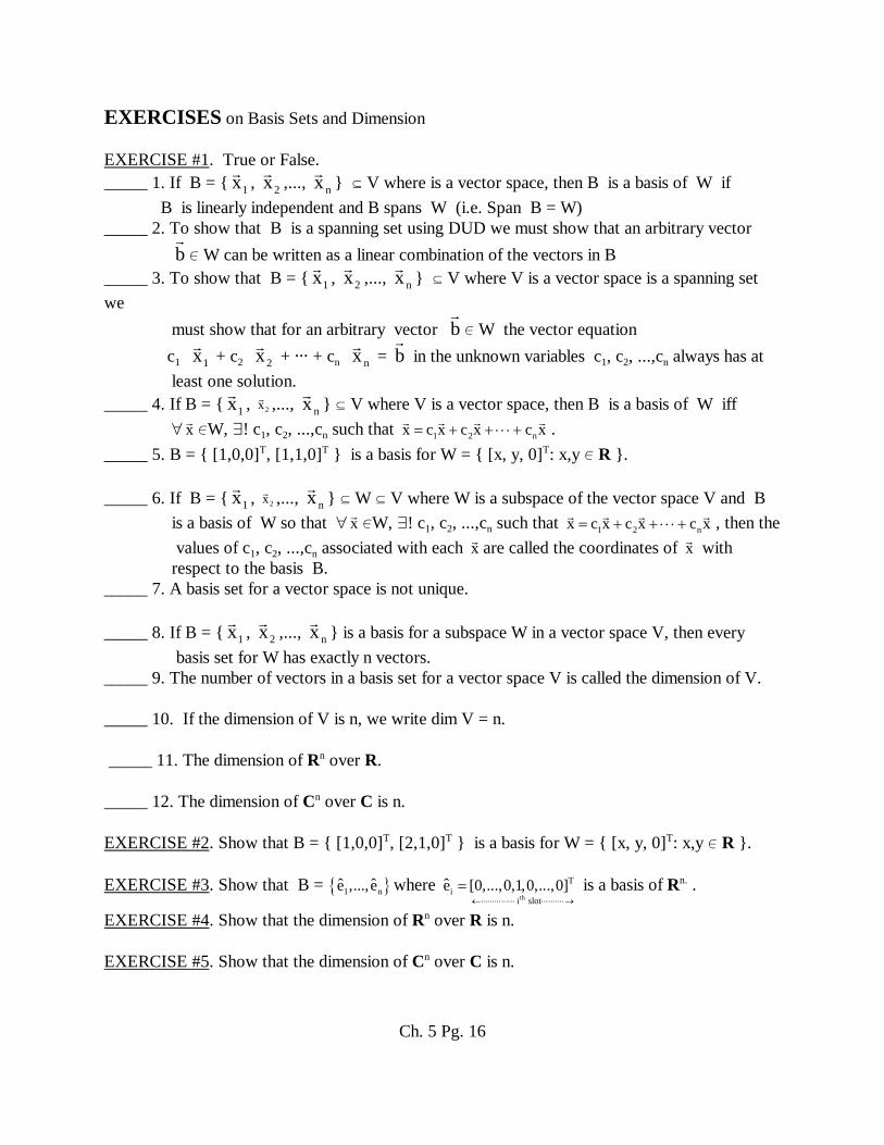
EXERCISES on Basis Sets and Dimension

EXERCISE #1. True or False._____ 1. If B = { , ,..., } V where is a vector space, then B is a basis of W if

x1x2

x n

B is linearly independent and B spans W (i.e. Span B = W)_____ 2. To show that B is a spanning set using DUD we must show that an arbitrary vector W can be written as a linear combination of the vectors in B

b

_____ 3. To show that B = { , ,..., } V where V is a vector space is a spanning setx1

x2x n

we must show that for an arbitrary vector W the vector equation

b

c1 + c2 + + cn = in the unknown variables c1, c2, ...,cn always has at x1

x2x n

b

least one solution._____ 4. If B = { , ,..., } V where V is a vector space, then B is a basis of W iff

x1 2xx n

W, ! c1, c2, ...,cn such that .x 1 2 nx c x c x c x

_____ 5. B = { [1,0,0]T, [1,1,0]T } is a basis for W = { [x, y, 0]T: x,y R }.

_____ 6. If B = { , ,..., } W V where W is a subspace of the vector space V and B x1 2x

x n

is a basis of W so that W, ! c1, c2, ...,cn such that , then thex 1 2 nx c x c x c x

values of c1, c2, ...,cn associated with each are called the coordinates of with x x

respect to the basis B._____ 7. A basis set for a vector space is not unique.

_____ 8. If B = { , ,..., } is a basis for a subspace W in a vector space V, then everyx1

x2x n

basis set for W has exactly n vectors._____ 9. The number of vectors in a basis set for a vector space V is called the dimension of V.

_____ 10. If the dimension of V is n, we write dim V = n.

_____ 11. The dimension of Rn over R.

_____ 12. The dimension of Cn over C is n.

EXERCISE #2. Show that B = { [1,0,0]T, [2,1,0]T } is a basis for W = { [x, y, 0]T: x,y R }.

EXERCISE #3. Show that B = where is a basis of Rn. . 1 nˆ ˆe ,..., eth

Ti

i slote [0,...,0,1,0,...,0]

EXERCISE #4. Show that the dimension of Rn over R is n.

EXERCISE #5. Show that the dimension of Cn over C is n.

Ch. 5 Pg. 16

Ch. 5 Pg. 17

A SERIES OF CLASS NOTES TO INTRODUCE LINEAR AND NONLINEAR PROBLEMSTO ENGINEERS, SCIENTISTS, AND APPLIED MATHEMATICIANS

LINEAR CLASS NOTES:A COLLECTION OF HANDOUTS FOR

REVIEW AND PREVIEW OF LINEAR THEORY

INCLUDING FUNDAMENTALS OF LINEAR ALGEBRA

CHAPTER 6

Preview of the

Theory of Abstract Linear Equations

of the First Kind

1. Linear Operator Theory

2. Introduction to Abstract Linear Mapping Problems

Ch. 6 Pg. 1

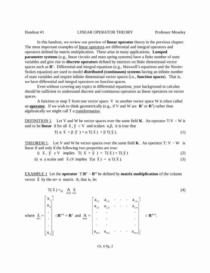
Handout #1 LINEAR OPERATOR THEORY Professor Moseley

In this handout, we review our preview of linear operator theory in the previous chapter. The most important examples of linear operators are differential and integral operators andoperators defined by matrix multiplication. These arise in many applications. Lumpedparameter systems (e.g., linear circuits and mass spring systems) have a finite number of statevariables and give rise to discrete operators defined by matrices on finite dimensional vectorspaces such as Rn. Differential and integral equations (e.g., Maxwell’s equations and the Navier-Stokes equation) are used to model distributed (continuum) systems having an infinite numberof state variables and require infinite dimensional vector spaces (i.e., function spaces). That is,we have differential and integral operators on function spaces.

Even without covering any topics in differential equations, your background in calculus should be sufficient to understand discrete and continuous operators as linear operators on vectorspaces.

A function or map T from one vector space V to another vector space W is often calledan operator. If we wish to think geometrically (e.g., if V and W are R2 or R3) rather thanalgebraically we might call T a transformation.

DEFINITION 1. Let V and W be vector spaces over the same field K. An operator T:V W issaid to be linear if for all , V and scalars α,β, it is true that

x y T( α + β ) = α T( ) + β T( ). (1)

x y x y

THEOREM 1. Let V and W be vector spaces over the same field K. An operator T: V W islinear if and only if the following two properties are true:

i) , ε V implies T( + ) = T( ) + T( ) (2)x y x y x y

ii) α a scalar and εV implies T(α ) = α T( ). (3)x x x

EXAMPLE 1 Let the operator T:Rn Rm be defined by matrix multiplication of the column vector by the m× n matrix A; that is, let

x

T( ) =df (4)x A

mxn

xnx1

where Rnx1 = Rn and = Rm×n.x

xx

x

nx1

1

2

n

mxnA

1,1 1,2 1,n

2,1 2,2 2,n

m,1 m,1 m,n

a a aa a a

a a a

Ch. 6 Pg. 2

Then T is a linear operator.

EXAMPLE 2 Let I = (a,b). The operator D:C1(I,R) C(I,R) be defined by

D(f) =df (5)dfdx

where f ε C1(I,R) = {f:I R: exists and is continuous on I} anddfdx

C(I,R) ={f:I R : f is continuous on I}. Then D is a linear operator. We may restrict D to A (I, R) ={f:I R:f is analytic on I} so that D:A (I, R) A (I, R) maps a vector space back toitself.

DEFINITION #2. Let T:VW be a mapping from a set V to a set W. The set R(T) = { y W: there exists an xV such that y = T(x) } is called the range of T. If W has anadditive structure (i.e., a binary operation which we call addition) with an additive identity whichwe call 0, then the set N(T) = {xV: T(x) = 0} is called the null set of T (or nullity of T).

If T is a linear operator from a vector space V to another vector space W, we can say more.

THEOREM #2 Let T:VW be a linear operator from a vector space V to a vector space W. The range of T R(T) = { W: there exists an V such that = T( ) }, is a subspace of W

y x y xand the null set of T, N(T) = { V: T( ) = 0} is a subspace of V.

x x

We rename these sets.

DEFINITION #3. Let T:VW be a linear operator from a vector space V to another vectorspace W. The set R(T) = { W: there exists an V such that = T( ) } is called the

y x y xrange space of T and the set N(T) = { V: T( ) = 0} is called the null space of T. .

x x

Ch. 6 Pg. 3

Handout #2 INTRODUCTION TO ABSTRACT Professor MoseleyLINEAR MAPPING PROBLEMS

We consider the (abstract) equation (of the first kind)

T( ) = (Nonhomogeneous) (1)x

b

where T is a linear operator from the vector space V to the vector space W ( T:V W ). Weview (1) as a mapping problem; that is, we wish to find those that are mapped by T to . x's b

THEOREM #1. For the nonhomogeneous equation (1) there are three possibilities:1) There are no solutions.2) There is exactly one solution.3) There are an infinite number of solutions.

THEOREM #2. For the homogeneous equation

T( ) = (Homogeneous) (2)x

0

there are only two possibilities:1) There is exactly one solution, namely = ; that is the null space of T (i.e. the set of

x0

vectors that are mapped into the zero vector) is N(T) = { }.0

2) There are an infinite number of solutions. If the null space of T is finite dimensional, say has dimension k ε N, then the general solution of (2) is of the form

= c1 + +ck = (3)x x1

x k

k

i ii 1

c x

where B = { ,, } is a basis for N(T) and ci, i=1,...,k are arbitrary constants.x1

x k

THEOREM #3. The nonhomogeneous equation (1) has at least one solution if is b

contained in the range space of T, R(T), (the set of vectors W for which there exist V w v

such that T[ ] = ). If this is the case, then the general solution of (1) is of the formv w

= + (4)x x p

x h

where is a particular (i.e. any specific) solution to (1) and is the general (e.g. ax p

x h

parametric formula for all) solution(s) of (2). If N(T) is finite dimensional then

= + = + c1 + +ck = + (5)x x p

x hx p

x1x k

x p c xi ii 1

k

Ch. 6 Pg. 4

where B = { ,, } is a basis of N(T). For the examples, we assume some previousx1

x k

knowledge of determinants and differential equations. Even without this knowledge, youshould get a feel for the theory. And if you lack the knowledge, you may wish to reread thishandout after obtaining it.

EXAMPLE 1 OPERATORS DEFINED BY MATRIX MULTIPLICATION We now apply the general linear theory to operators defined by matrix multiplication. We lookfor the unknown column vector = [x1,x2,,xn]T. (We use the transpose notation on a row

xvector to indicate a column vector to save space and trees.) We consider the operator T[ ] = A where A is an m×n matrix.

x x

THEOREM 4. If is in the column (range) space of the matrix (operator) A, then the generalb

solution to the nonhomogeneous system of algebraic equation(s)

= (6)Amxn

xnx1

b

mx1

can be written in the form

= + c1 + +ck = + (7)x x p

x1x k

x p c xi ii 1

k

where is a particular ( i.e. any) solution to (6) andx p

= c1 + +ck = (8)x h

x1x k c xi i

i 1

k

is the general solution (i.e. a parametric formula for all solutions) to the complementaryhomogeneous equation

= (9)Amxn

xnx1 mx1

0

Here B = { ,, } is a basis for the null space N(T) ( also denoted by N(A) ) which hasx1

x k

dimension k. All of the vectors , ,, can be founded together using the computationalpx x1 kx

technique of Gauss Elimination. If N(T) = { }, then the unique solution of = is 0 A

mxn nx1x

b

mx1

x p

(and the unique solution to is = ).mx1mxnnx10A x x h

0

nx1

THEOREM 5. If n = m, then we consider two cases (instead of three) for equation (6): 1) det A 0 so that A is nonsingular; then the matrix A has a unique inverse, A1 (which is almost never computed), and for any Rm, = always has the unique solution

b A

nxn

xnx1

b

nx1

Ch. 6 Pg. 5

=A1 . Thus the operator is one-to-one and onto so that any vector is x b

T(x) = Ax b

always in the range space R(A) and only the vector =A1 . maps to it. Again, the matrix x

b

A defines an operator that is a one-to-one and onto mapping from Rn to Rn (or Cn to Cn). 2) det A = 0 so that A is singular; then either there is no solution or if there is a solution, then there are an infinite number of solutions. Whether there is no solution or an infinite numbers of solutions depends on , specifically, on whether εR(A) or not. The operator

b

b

defined by tha matrix A is not one-to-one or onto and the dimension of N(A) is greater than or equal to one.

EXAMPLE 2 LINEAR DIFFERENTIAL EQUATIONSTo avoid using x as either the independent or dependent variable, we look for the unknownfunction u (dependent variable) as a function of t (independent variable). We let the domain of ube I = (a,b) and think of the function u as a vector in an (infinite dimensional) vector (function)space.

THEOREM 6. If g is in the range space R(L) of the linear differential operator L (i.e. g ε R(L) ) then the general solution to the nonhomogeneous equation

L[ u(t) ] = g(t) t I (10)

can be written in the form

u(t) = up(t) + uh(t) (11)

where up is a particular solution to (10) and uh is the general solution to the homogeneousequation

L[ u(t) ] = 0 t I (12)

Special cases:1) L[ u(t) ] = u" + p(t)u + q(t)u. Second Order Scalar Equation.

For this case, we let I = (a,b) and L:A (I,R) A (I,R). It is known that the dimension ofthe null space is two so that

uh(t) = c1u1(t) + c2u2(t).

2) L[ u(t) ] = po(t) + + pn(t) u(t) nth Order Scalar Equation.n

n

d udt

Again we let I = (a,b) and L:A (I,R) A (I,R). For this case, the dimension of the null space is n so that

Ch. 6 Pg. 6

uh(t) = c1 u1(t) + +cn un(t) = .c u (t)i ii 1

n

3) L[ ] = First Order System ("Vector" Equation)u(t) du

dt

P (t)u(t)

nxn

Again we let I = (a,b), but now L:A (I,Rn) A (I,Rn) where A (I,Rn) =

{ }; nu(t) : I R

that is the set of all time varying "vectors". Here the word "vector" means an n-tuple of functions. We replace (10) with

L[ ] = u(t) g(t)

and (12) with L[ ] = .

u(t)0

Then = + u(t) u (t)p

u (t)h

where = c1 + + cn (i.e. the null space is n dimensional).

u (t)hu (t)1

u (t)n

Ch. 6 Pg. 7

A SERIES OF CLASS NOTES TO INTRODUCE LINEAR AND NONLINEAR PROBLEMSTO ENGINEERS, SCIENTISTS, AND APPLIED MATHEMATICIANS

LINEAR CLASS NOTES:A COLLECTION OF HANDOUTS FOR

REVIEW AND PREVIEW OF LINEAR THEORY

INCLUDING FUNDAMENTALS OF LINEAR ALGEBRA

CHAPTER 7

Introduction to

Determinants

1. Introduction to Computation of Determinants

2. Computation Using Laplace Expansion

3. Computation Using Gauss Elimination

4. Introduction to Cramer’s Rule

Ch. 6 Pg. 1

Handout #1 INTRODUCTION TO COMPUTATION OF DETERMINANTS Prof. Moseley

Rather than give a fairly complicated definition of the determinant in terms of minors andcofactors, we focus only on two methods for computing the determinant function det:Rn×nR (or

det:CnxnC). Let A= . The we define det(A) = adbc. Later we will show that a bc d

A1 = . For ARn×n (or Cn×n), we develop two methods for computinga b a b1 1c d c dad bc det A

det(A): Laplace Expansion and Gauss EliminationBut first, we give (without proof) several properties of determinants that aid in their

evaluation.

THEOREM. Let ARn×n (or Cn×n). Then1. (ERO's of type 1) If B is obtained from A by exchanging two rows, then det(B) = det(A).2. (ERO's of type 2) If B is obtained from A by multiplying a row of A by a0, then det(B) = a det(A).3. (ERO's of type 3) If B is obtained from A by replacing a row of A by itself plus a scalarmultiple of another row, then det(B) = det(A).4. If U is the upper triangular matrix obtained from A by Gauss elimination (forward sweep) usingonly ERO's of type 3, then det(A) = det(U)5. If URn×n (or Cn×n) is upper triangular, then det(U) is equal to the product of the diagonalelements.6. If A has a row (or column) of zeros, then det(A) = 0.. 7. If A has two rows (or columns) that are equal, then det(A) = 0.. 8. If A has one row (column) that is a scalar multiple of another row (column), then det(A) = 0.. 9. det(AB) =det(A) det(B)..10.If det(A) 0, then det(A1) = 1/det(A).11. det(AT) = det(A).

EXERCISES on Introduction of Computation of Determinants

EXERCISE #1. True or False.

_____ 1. If A= , then det(A) = adbca bc d

_____ 2.If A= , then A1 = .a bc d

a b1c dad bc

_____ 3.If ARn×n (or Cn×n), there are (at least) two methods for computing det(A)._____ 4. If ARn×n (or Cn×n), Laplace Expansionis one method for computing det(A)_____ 5. 3.If ARn×n (or Cn×n), use of Gauss Elimination is one method for computing det(A).

Ch. 6 Pg. 2

_____ 6. If ARn×n (or Cn×n) and B is obtained from A by exchanging two rows, then det(B) = det(A)._____ 7. If ARn×n (or Cn×n) and B is obtained from A by multiplying a row of A by a0, then det(B) = a det(A)._____ 8. If ARn×n (or Cn×n) and B is obtained from A by replacing a row of A by itself plus a scalar multiple of another row, then det(B) = det(A)._____ 9. If ARn×n (or Cn×n) and U is the upper triangular matrix obtained from A by Gauss elimination (forward sweep) using only ERO's of type 3, then det(A) = det(U)_____ 10. If ARn×n (or Cn×n) and URn×n (or Cn×n) is upper triangular, then det(U) is equal to the product of the diagonal elements._____ 11. If ARn×n (or Cn×n) and A has a row of zeros, then det(A) = 0._____ 12. If ARn×n (or Cn×n) and A has a column of zeros, then det(A) = 0. _____ 13. If ARn×n (or Cn×n) and A has two rows that are equal, then det(A) = 0. _____ 14. If ARn×n (or Cn×n) and A has two columns that are equal, then det(A) = 0. _____ 15. If ARn×n (or Cn×n) and A has one row that is a scalar multiple of another row, then det(A) = 0. _____ 16. If ARn×n (or Cn×n) and A has one column that is a scalar multiple of another column, then det(A) = 0. _____ 17. If A,BRn×n (or Cn×n) then det(AB) =det(A) det(B).._____ 18. If ARn×n (or Cn×n) and det(A) 0, then det(A1) = 1/det(A)._____ 19. If ARn×n (or Cn×n), thjen det(AT) = det(A).

EXERCISE #2. Compute det A where 0 5A

0 1

EXERCISE #3. Compute det A where 1 2A

3 1

EXERCISE #4. Compute det A where 1 iA

i 1

EXERCISE #5. Compute det A where 1 iA

i 0

EXERCISE #6. Compute A1 if 2 5A

3 7

EXERCISE #7. Compute A1 if 2 1A

5 3

EXERCISE #8. Compute A1 if 1 iA

i 2

EXERCISE #9. Compute A1 if 1 iA

i 0

EXERCISE #10. Compute A1 if 0 5A

0 1

EXERCISE #11. Compute A1 if 1 2A

3 1

EXERCISE #12. Compute A1 if 1 iA

i 1

Ch. 6 Pg. 3

Handout #2 COMPUTATION USING LAPLACE EXPANSION Professor Moseley

We give an example of how to compute a determinant using Laplace expansion..

EXAMPLE. Compute det(A) where A= using Laplace expansion..

2 1 0 01 2 1 0

0 1 2 10 0 1 2

Solution: Expanding in terms of the first row we havc

det(A) = = 2 (1)

2 1 0 01 2 1 0

0 1 2 10 0 1 2

2 1 01 2 1

0 1 2

1 1 00 2 10 1 2

+(0) (0)

1 2 00 1 10 0 2

1 2 10 1 20 0 1

so the last two 3x3's are zero. Hence expanding the first remaining 3x3 in terms of the first rowand the second interms of the first column we have

det(A) = 2 (1) 2 1 1 1 1 2( 1) (0)1 2 0 2 0 1

2 1 1 0 1 0(0) (0)1 2 1 2 2 1

= 2[(41) +(2)] + [4 1] = 2 + 3 = 5

Ch. 6 Pg. 4

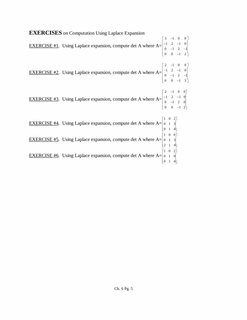
EXERCISES on Computation Using Laplace Expansion

EXERCISE #1. Using Laplace expansion, compute det A where A= 3 1 0 01 2 1 0

0 1 2 10 0 1 2

EXERCISE #2. Using Laplace expansion, compute det A where A= 2 1 0 01 2 1 0

0 1 2 10 0 1 3

EXERCISE #3. Using Laplace expansion, compute det A where A= 2 1 0 01 2 1 0

0 1 2 00 0 1 2

EXERCISE #4. Using Laplace expansion, compute det A where A= 1 0 20 1 30 1 4

EXERCISE #5. Using Laplace expansion, compute det A where A= 1 0 00 1 32 1 4

EXERCISE #6. Using Laplace expansion, compute det A where A= 1 0 20 1 00 1 4

Ch. 6 Pg. 5

Handout #3 COMPUTATION USING GAUSS ELIMINATION Professor Moseley

We give an example of how to compute a determinant using Gauss elimination.

EXAMPLE. Compute det(A) where A= using Gauss elimination.

2 1 0 01 2 1 0

0 1 2 10 0 1 2

RecallTHEOREM. Let ARn×n (or Cn×n). Then3. (ERO's of type 3) If B is obtained from A by replacing a row of A by itself plus a scalarmultiple of another row, then det(B) = det(A).4. If U is the upper triangular matrix obtained from A by Gauss elimination (forward sweep) usingonly ERO's of type 3, then det(A) = det(U).

2 1

2 1 0 0R (1/ 2)R 1 2 1 0

0 1 2 10 0 1 2

3 2

2 1 0 00 3 / 2 1 0

R (2 / 3)R 0 1 2 10 0 1 2

3 2

2 1 0 00 3/ 2 1 00 0 4 / 3 1

R (3/ 4)R 0 0 1 2

2 1 0 00 3 / 2 1 00 0 4 / 3 10 0 0 5 / 4

Since only ERO's of Type 3 were used, we have det(A) = det(U) = 2(3/2)(4/3)(5/4) = 5.

EXERCISES on Computation Using Gauss Elimination

EXERCISE #1. Using Gauss elimination, compute det A where A= 3 1 0 01 2 1 0

0 1 2 10 0 1 2

EXERCISE #2. Using Gauss elimination, compute det A where A= 2 1 0 01 2 1 0

0 1 2 10 0 1 3

EXERCISE #3. Using Gauss elimination, compute det A where A= 2 1 0 01 2 1 0

0 1 2 00 0 1 2

Ch. 6 Pg. 6

Handout #1 INTRODUCTION TO CRAMER’S RULE Prof. Moseley

Cramer’s rule is a method of solving when A is square and the determinant of AAx = b

which we denote by D 0. The good news is that we have a formula. The bad news is that,computationally, it is not efficient for large matrices and hence is never used when n > 3. Let Abe an nxn matrix and A = [aij]. Let be nx1 column vectors andT

1 2 nx = [x ,x ,...,x ] and b

. Now let Ai be the matrix obtained from A by replacing the ith column of a byi ix = [x ] and b = [b ]

the column vector . Denote the determinant of Ai by Di. Then xi = Di/D so thatb

.T T1 2 n ix = [x ,x ,..., x ] = [D / D]

EXERCISES on Introduction to Cramer’s Rule

EXERCISE #1. Use Cramer’s rule to solve where and Ax = b 2 3

A3 5

2b =

3

EXERCISE #2. Use Cramer’s rule to solve where and Ax = b 2 3

A3 5i

i

2b =

3

EXERCISE #3.Use Cramer’s rule to solve where Ax = b 1 1 1 5

A 1 1 3 and b 12 1 1 3

EXERCISE #4. Use Cramer’s rule to solve x1 + x2 + x3 + x4 = 1 x1 + 2x2 + x3 = 0 x3 + x4 = 1 x2 + 2x3 + x4 = 1

Ch. 6 Pg. 7

A SERIES OF CLASS NOTES TO INTRODUCE LINEAR AND NONLINEAR PROBLEMSTO ENGINEERS, SCIENTISTS, AND APPLIED MATHEMATICIANS

LINEAR CLASS NOTES:A COLLECTION OF HANDOUTS FOR

REVIEW AND PREVIEW OF LINEAR THEORY

INCLUDING FUNDAMENTALS OF LINEAR ALGEBRA

CHAPTER 8

Inner Product and

Normed Linear Spaces

1. Normed Linear Spaces

2. Inner Product Spaces

3. Orthogonal Subspaces

4. Introduction to Error Analysis in Normed Linear Spaces

Ch. 8 Pg. 1

Handout #1 NORMED LINEAR SPACES Prof. Moseley

Since solving linear algebraic equations for a field K require only a finite number of exactalgebraic steps, any field will do. However, actually carrying out the process usually involvesapproximate arithmetic and hence approximate solutions. In an infinite dimensional vector spacethe solution process often requires an infinite process that converges. Hence the vector space (orits field) must have additional properties. Physicists and engineers think of vectors as quantitieswhich have length and direction. Although the notion of direction can be discusssed, thedefinition of a vector space does not include the concept of the length of a vector. Theabstraction of the concept of length of a vector is called a norm and vector spaces (also calledlinear spaces) which have a norm (or length) are called normed linear spaces. Having thenotion of length in a vector space gives us the notion of a unit vector (i.e. a vector of length one).

DEFINITION #1. A normed linear space is a real or complex vector space V on which a normhas been defined. A norm (or length) is a function such that:V { : 0} R R

1) x 0, x V

if and only if x 0 x 0

2) scalars αx x x V

3) (this is called the triangle in equality)1 2 1 2 1 2x x x x x ,x V

Note that the zero vector is the only vector with zero length. For all other vectors 0

x

we have . Hence for each non zero we can define the unit vector x 0 x

. (1)1 xu u(x) xx x

LEMMA #1. If V, and , then . x V, x 0 1 xu u(x) x

x x

u 1

Proof. Let . Then1 xu u(x) xx x

Statement Reason

Definition of 1u xx

u

= Property (2) above 1 xx

= Algebraic Properties of Rxx

= 1 Algebraic Properties of R.

Ch. 8 Pg. 2

THEOREM #1. If , then can be written as where is a unit vector in thex 0 x x x u

u

direction of and gives the length of .x x x

Proof idea. That is the length or norm of follows from the definition of as a norm orx x x

length. Since , and we define as before as the unit vector wex 0

x 0 u 1 xu u(x) x

x x

see that is a positive scalar multiple of so that it is pointed in the same “direction” as . Tou x x

show that is left as an exercise. QEDx x u

The abstraction of the notion of distance between two points in a set (or vector space) iscalled a metric.

DEFINITION #2. A metric space is a set S on which a metric has been defined. A metric (ordistance between) on S is a function ρ:S×SR+={αRα0} such that

1) ρ(x,y)0 f x,yS.ρ(x,y) =0 if and only if x=y.

2) ρ(x,y) = ρ(y,x).3) ρ(x,z) ρ(x,y) + ρ(y,z) (this is also called the triangle in equality)

THEOREM #2. Every normed vector space is a metric space with the metric .(x, y) x y

However, we note that a metric space need not be a vector space. Geometrically in R3, ρ is thedistance between the tips of the position vectors and . A metric yields the notion of ax y

topology, but we need not develop this more general concept. However, to discuss approximatesolutions, we do need the notion of completeness. Although it could be developed in a moregeneral context, we are content to discuss complete vector spaces.

DEFINITION #3. A Cauchy sequence of vectors is a sequence in a normed linearn 1n{x

}space V such that for any ε>0, there exists N with < ε whenever m,n>N.

xnxm

Thus get close together when n and m are large. m nx and x

DEFINITION #4. A sequence of vectors in a vector space V is convergent if there existn 1n{x

}such that for any ε>0, there exists N with < ε whenever n>N.

x xnx

DEFINITION #5. A vector space is complete if every Cauchy sequence of vectors converges. ABanach Space is a complete normed linear space.

Ch. 8 Pg. 3

The concepts of metric (or topology) and completeness are essential for computing limits; forexample, in the process of computing approximate solutions and obtaining error estimates.Completeness does for a vector space what R does for Q (which are just special cases). It makessure that there are no holes in the space so that Cauchy sequences (that look like they ought toconverge) indeed have a vector to converge to. If we wish to solve problems in a metric space Sand S is not complete, we can construct the completion of S which we usually denote by . SThen, since is complete, we can obtain approximate solutions. S

Ch. 8 Pg. 4

Handout #2 INNER PRODUCT SPACES Prof. Moseley

Recall that to determine if two vectors in R3 are perpendicular, we compute the dotproduct. The abstraction of the notion of dot product in an abstract vector space is called aninner product. Vector spaces on which an inner product is defined are called inner productspaces. As we will see, in an inner product space we have not only the notion of two vectorsbeing perpendicular but also the notions of length of a vector and a new way to determine if aset of vectors is linearly independent.

DEFINITION #1. An inner product space is a real or complex vector space V on which aninner product is defined. A inner product is a function (,): V × VR such that ____

1) (x, y) (y,x) x, y V

(the bar over the inner product indicates complex conjugate. If V is a real vectorspace, it is not necessary and we see that the inner product is commutative for realvector spaces.)

2) and scalars α.( x, y) (x, y) x, y V

3) .1 2 11 2 1 2(x x , y) (x , y) (x , y) x ,x , y V

(Properties 2 and 3) say that the inner product is linear in the first slot.)4) (x, x) 0 x V

(x,x) 0 iff x 0

If V is an inner product space we define a mapping, by: V { : 0} R R

. (1)x (x,x)

THEOREM #1. given by (1) defines a norm on any inner product space and hencex (x,x)

makes it into a normed linear space. (See the previous handout)

DEFINITION #2. A Hilbert space is a complete, inner product space.

Again, the concept of completeness in a vector space is an abstraction of what R does for Q. R iscomplete; Q is not.

EXAMPLE (THEOREM). Let V = Rn and define the inner product by n

Ti i

i 1

(x, y) x y x y

where . Note that we can define the inner product in Rn in terms of matrixT T1 nx [x ,..., x ]

multiplication. Note also . We can then prove (i.e. verify) that defines anT(x, y) y x T(x, y) x y

inner product (i.e. satisfies the properties in the definition of an inner product).

Ch. 8 Pg. 5

Proof of 2). Let , thenT T1 nx [x ,..., x ]

T T1 ny [y ,..., y ]

Statement Reason = definition of inner product for Rn. ( x, y)

Tx y

= notation and definition of transpose

1

1 n

n

y

( [x ,..., x ])

y

= definition of scalar multiplication

1

1 n

n

y

[ x ,..., x ]

y

= (αx1)y1 + (αx2)y2 ++ (αxn)yn definition matrix multiplication = α(x1y1 + x2y2 ++ xnyn) properties real numbers = definition of matrix multiplicationT(x y)

= definition of inner product (x, y)

QED

Note that in Rn we have

. (2)n

T 2 2 21 n i

i 1

x (x,x) x x x x x

In R3 we know that two vectors are perpendicular if their dot product is zero. We abstract thisidea by defining two vectors in an inner product space to be orthogonal (rather than use the wordperpendicular) if their inner product is zero.

DEFINITION #3. The row vectors =[x1,x2,...,xn] and =[y1,y2,...,yn] in Rn are orthogonal ifx y

(and only if) .T(x, y) x y 0

Pythagoras Extended. In R3 (or any real inner product space) we might define two vectors to beperpendicular if they satisfy the Pythagorean theorem; that is if

. (3)2 2 2x y x y ( (x, y))

Since , (3) may be rewritten asx y (x y)

Ch. 8 Pg. 6

(x, x) (y, y) (x y,x y)

= (4)(x,x) 2(x, y) (y, y)

(since the inner product is commutative; Cn is different.)

THEOREM #2. and in Rn are perpendicular iff they are orthogonal.x y

DEFINITION #4. is a unit vector (i.e. a vector of length one) in the direction of thexux

nonzero vector ( has no direction). Hence any nonzero vector can be written asx 0

x

where is the magnitude or length and is a unit vector in the direction ofxx xx

x xux

.x

DEFINITION #5. The cosine of the acute angle θ ( 0 θ π) between two nonzero vectors x

and Rn isy

(5)T(x, y) x ycos( )

x y x y

Note: This is often used as the geometric definition of dot product in R3.To show that (5) does yield θ in R3 we first extend the concept of projection.

DEFINITION #6. The vector projection of a vector in the direction of a non-zero vector b

a

is given by (a,b)p b cos

a

scalar

ap b cosa

magnitude unit vector giving direction of p

of p

2

(a,b) a (a,b) aa a a

The magnitude of is called the scalar projection of in the direction of p b

a

Ch. 8 Pg. 7

Handout #3 ORTHOGONAL SUBSPACES Prof. Moseley

We first review the definition, a theorem, and the test for a subspace.

DEFINITION #1. Let W be a nonempty subset of a vector space V. If for any vectors , W and scalars α,β K (recall that normally the set of scalars K is either R or C), we

x yhave that α + β W, then W is a subspace of V.

x y

THEOREM #1. A nonempty subset W of a vector space V is a subspace of V if and only if for , V and α K (i.e. α is a scalar) we have.

x y i) , W implies + W, andx y x y

ii) W implies α W.x x

TEST FOR A SUBSPACE. Theorem #1 gives a good test to determine if a given subset of avector space is a subspace since we can test the closure properties separately. Thus if W Vwhere V is a vector space, to determine if W is a subspace,we check the following three points.

1) Check to be sure that W is nonempty. (We usually look for the zero vector since if there is W, then 0 = must be in W. Every vector space and every subspace x x 0

must contain the zero vector.)2) Let and be arbitrary elements of W and check to see if + is in W.

x y x y (Closure of vector addition) 3) Let be an arbitrary element in W and check to see if α is in W.

x x (Closure of scalar multiplication).

DEFINITION #2 Let W1 and W2 be subspaces of a vector space V. Then the sum of W1 andW2 is defined as W1 +W2 ={ : }.1 2x x

1 1 2 2x W and x W

THEOREM #2 Let W1 and W2 be subspaces of a vector space V. Then the sum of W1 and W2is subspace of V.

DEFINITION #3 Let W1 and W2 be subspaces of a vector space V such that. Then the sum of W1 and W2 defined as W1 +W2 ={ : 1 2 0W W

1 2x x

} is a direct sum which we denote by 1 1 2 2x W and x W 1 2W W

THEOREM #3 Let W1 and W2 be subspaces of a vector space V and . Then for every vector in V there exist unique 1 2 1 2 1 1 2 2:V = W W = x + x x W and x W x

vectors W1 and W2 such that .1x 2x1 2x = x + x

Ch. 8 Pg. 8

DEFINITION #4 Let W1 and W2 be subspaces of a real inner product space V with inner product (,). W1 and W2 are said to be orthogonal to each other if + x W1 and x + y y

W2, we have ( , ) = 0. We write W1 2 W2.x y

THEOREM #4. If A Rm×n, then its row space is orthogonal to its null space and its column space is orthogonal to its left null space. We write R(AT) 2 N(A) and R(A) 2 N(AT).

DEFINITION #5 Let W be a subspace of a real inner product space V with inner product (,).The orthogonal complement of W is the set W 2 = { V: ( , ) = 0 W}.y x y x

THEOREM #5. Let W be a subspace of a real inner product space V with inner product (,).Then the orthogonal complement of W, W 2 = { V: ( , ) = 0 W}, is a subspace.y x y x

THEOREM #6. Let W be a subspace of a real inner product space V with inner product (,).Then the orthogonal complement of W 2 is W. We write (W 2) 2 = W.

THEOREM #7. If A Rm×n, then its row space is the orthogonal complement of its null space and the null is the orthogonal complement to the row space. We write R(AT) 2 = N(A) and N(A) 2 = R(AT). Similarly, R(A) 2 = N(AT) and N(AT) 2 = R(A).

THEOREM #8. Let W be a nonempty subset of a real inner product space V with inner product (,). Then V is the direct sum of W and W 2 , V = W W 2.

THEOREM #9. If A Rm×n, then Rn = R(AT) N(A) and Rm = R(A) N(AT).

Ch. 8 Pg. 9

Handout #4 INTRODUCTION TO ERROR ANALYSIS Prof. MoseleyIN NORMED LINEAR SPACES

In vector spaces where the concept of length or norm (as well as direction) is available, we can talk about approximate solutions to the mapping problem

T( ) = (1)u b

where T is a linear operator from V to W; T:VW where V and W are normed linear spaces. Let V be an approximate solution of (1) and V be the exact solution which we assume au eu

to exist and be unique. A measure of how good a solution is is given by the norm or length of au

the error vector in V,

;v e aE u u

that is,.V v e aE E u u

If T is invertible (e.g., if T:RnRn, is defined by a matrix, T( ) = A and detA0), then x x

1 1 1V v e a a aE E u u T (b) T (b ) T (b b )

where . (The inverse of a linear operator, if it exists, is a linear operator.) By a well-a ab T(u )

known theorem in analysis,

1 1a aT (b b ) T b b

where T-1 is the norm of the operator T-1 which we assume to be finite. If an a priori “estimate” (i.e., bound) of T-1, say T-1 C, can be obtained, then an “estimate of” (i.e., bound for) EV can be obtained by first computing . Even without an estimate of (bound ab b

for) T-1, we may use

E = EW = . b ba = b T(ua)a ab b b T(u )

where

; W a aE b b b T(u )

is a measure of the error for . After all, if , then so that EW = 0. We call EW au a eu u aT(u ) b

the error vector in W. Note that this error vector (and hence E) can always be computed whereas usually can not. (If is known, then the exact solution is VE

VE

e a Vu u E

Ch. 8 Pg. 10

known and there is no need for an approximate solution.) In fact, E can be computed independent of whether (1) has a unique solution or not. We refer to a solution that minimizes E = EW as a least error solution. If (1) has one or more solutions, then these are all least error solutions since they all give E = 0. On the other hand, if (1) has no solution, then choosing tou

minimize E gives a “best possible” solution. Under certain conditions, it is unique.

Ch. 8 Pg. 11

Handout #5 ORTHOGONAL BASIS AND BASIS SETS FOR Prof. MoseleyINFINITE DIMENSIONAL VECTOR SPACES

DEFINITION #1. Let S = { , ,..., } W V where W is a subspace of the inner product1x 2x kx

space V. Then S is said to be (pairwise) orthogonal if for all i,j we have { , ) = 0 for ij. If Six jx

is a basis of W, it is called an orthogonal basis. (This requires that S does not contain the zerovector.) An orthogonal basis is said o be othonormal if for alli, ix 0

If B = { , ,..., } V is an orthogonal basis for the inner product space V, then the1x 2x kx

coordinates for are particularly easy to compute. Let x V

. (1)1 1 2 2 k kx c x c x c x V

To find ci, take the inner product of both sides with .jx

. 1 1 2 2j j k k(x ,x) (x ,c x c x c x )

1 1 2 2j j j j k k(x ,x) (x ,c x ) (x ,c x ) (x ,c x )

1 1 2 2j j j k j k(x ,x) c (x ,x ) c (x ,x ) c (x ,x )

(2)j j j j(x , x) c (x ,x )

so that

. (3)j

jj j

(x ,x)c

(x ,x )

The concepts of a basis and orthogonal basis can be extended to infinite dimensionalspaces. We first extend the concepts of linear independence and spanning sets.

DEFINITION #2. An infinite set S in a vector space V is linearly independent if every finitesubset of S is linearly independent. Thus the countable set { , ,..., ,...} is linearly1x 2x kx

independent if Sn = { , ,..., } is linearly independent for all nN.1x 2x kx

DEFINITION #3. Let the countable set S = { , ,..., ,...} W V where W is a subspace1x 2x kx

of a vector space V. S is a Hamel spanning set for W if for all , there exists nN and c1, x W

c2, ..., cn such that . If V is a topological vector space (e.g. a normed linear1 1 2 2 n nx c x c x c x

space), then S is a Schauder spanning set for W if for all , there exist c1, c2, ..., cn,... suchx W

that .1 1 2 2 n n n nn 1

x c x c x c x c x

Ch. 8 Pg. 12

DEFINITION #3. Let B = { , ,..., } W V where W is a subspace of a vector space V. 1x 2x nx

B is a Hamel basis for W if it is linearly independent and a Hamel spanning set for W. If V is atopological vector space (e.g. a normed linear space), then B is a Schauder basis for W if it islinearly independent and a Schauder spanning set for W..

EXAMPLE. 1) Let B = {1, x, x2, x3, ...}. Then B is a Hamel basis for the set of all polynomialsP (R,R) and a Scauder basis for the set of all analytic functions with an infinite radius ofconvergence about x = 0. Note that both of these spaces are infinite dimensional.2) Let B = { , ,..., ,...} be an infinite linearly independent set in a real topological vector1x 2x nx

space. Then B is a Hamel basis for the subspace W1 = { = c1 +c2 ++cn : c1, c2, ,...cnR}x 1x 2x nx

of V and B is a Schauder basis for the subspace W2 = { = c1 +c2 ++cn +: c1, c2,x 1x 2x nx

,...cn,...R where the series converges} of V. Again, note that both of these spaces are infinitedimensional.

If B = { , ,..., ,...} V is an orthogonal basis for the Hilbert space H, then the coordinates1x 2x nx

for are particularly easy to compute. Let x H

. (4)1 1 2 2 n nx c x c x c x H

To find ci, take the inner product of both sides with .jx

. j j 1 1 2 2 n n(x ,x) (x ,c x c x c x )

j j 1 1 j 2 2 j n n(x ,x) (x ,c x ) (x ,c x ) (x ,c x )

j 1 j 1 2 j 2 n j n(x ,x) c (x , x ) c (x ,x ) c (x ,x )

(5)j j j j(x ,x) c (x ,x )

. (6)j

jj j

(x ,x)c (x ,x )

Note that this is the same formula as for the finite dimensional case.

Ch. 8 Pg. 13

A SERIES OF CLASS NOTES TO INTRODUCE LINEAR AND NONLINEAR PROBLEMSTO ENGINEERS, SCIENTISTS, AND APPLIED MATHEMATICIANS

LINEAR CLASS NOTES:A COLLECTION OF HANDOUTS FOR

REVIEW AND PREVIEW OF LINEAR THEORY

INCLUDING FUNDAMENTALS OF LINEAR ALGEBRA

CHAPTER 9

More on

Matrix Inverses

1. Re-introduction to Matrix Inverses

2. Computation Using Gauss Elimination

4. Formula for a 2x2 Matrix

Ch. 7 Pg. 1

Handout #1 RE-INTRODUCTION TO MATRIX INVERSES Prof. Moseley

Recall that if A and B are square, then we can compute both AB and BA. Unfortunately,these may not be the same.

THEOREM #1. If n >1, then there exists A, BR n×n such that AB BA. Thus matrixmultiplication is not commutative.

Thus AB=BA is not an identity. Can you give a counter example for n=2? (i.e. an examplewhere AB BA.)

DEFINITION #1. For square matrices, there is a multiplicative identity element. We definethe n×n matrix I by

= One's down the diagonal. Zero's everywhere else.Imxn

1 0 0

0 1 0

0 0 1

THEOREM #2. We have = = A Knxn Anxn

Inxn

Inxn

Anxn

Anxn

DEFINITION #2. If there exists B such that AB = I., then B is a right (multiplicative) inverseof A. If there exists C such that CA = I., then C is a left (multiplicative) inverse of A. If AB = BA = I, then B is a (multiplicative) inverse of A and we say that A is invertible. If B isthe only matrix with the property that AB = BA = I, then B is the inverse of A. If A has a uniqueinverse, then we say A is nonsingular and denote its inverse by A-1.

THEOREM #3. Th identity matrix is its own inverse.

Later we show that if A has a right and a left inverse, then it has a unique inverse. Hence weprove that A is invertible if and only if it is nonsingular. Even later, we show that if A has a right(or left) inverse, then it has a unique inverse. Thus, even though matrix multiplication is notcommutative, a right inverse is always a left inverse and is indeed the inverse. Some matriceshave inverses; others do not. Unfortunately, it is usually not easy to look at a matrix anddetermine whether or not it has a (multiplicative) inverse.

THEOREM #4. There exist A, BR n×n such that AI is invertible and B has no inverse.

Ch. 7 Pg. 2

INVERSE OPERATION. If B has a right and left inverse then it is a unique inverse ((i.e., B-1

such that B-1B = BB-1 = I) and we can define Right Division AB-1 and Left Division B-1A of Aby B (provided B-1 exists). But since matrix multiplication is not commutative, we do not know

that these are the same. Hence is not well defined since no indication of whether we meanAB

left or right division is given.

EXERCISES on Re-introduction to Matrix Inverses

EXERCISE #1. True or False._____ 1. If A and B are square, then we can compute both AB and BA. _____ 2. If n >1, then there exists A, BR n×n such that AB BA. _____ 3. Matrix multiplication is not commutative. _____ 4. AB=BA is not an identity._____ 5. For square matrices, there is a multiplicative identity element, namely the n×n matrix I,

given by = .nxnI

1 0 0

0 1 0

0 0 1

_____ 6. A Knxn we have = = Anxn

Inxn

Inxn

Anxn

Anxn

_____ 7. If there exists B such that AB = I., then B is a right (multiplicative) inverse of A.

_____ 8. If there exists C such that CA = I., then C is a left (multiplicative) inverse of A._____ 9. If AB = BA = I, then B is a multiplicative inverse of A and we say that A is invertible. _____ 10. If B is the only matrix with the property that AB = BA = I, then B is the inverse of A._____ 11. If A has a unique inverse, then we say A is nonsingular and denote its inverse by A-1._____ 12. The identity matrix is its own inverse. _____ 13. If A has a right and a left inverse, then it has a unique inverse. _____ 14. A is invertible if and only if it is nonsingular. _____ 15. If A has a right (or left) inverse, then it has a unique inverse. _____ 16. Even though matrix multiplication is not commutative, a right inverse is always a left inverse._____ 17. The inverse of a matrix is unique._____ 18. Some matrices have inverses; others do not. _____ 19. It is usually not easy to look at a matrix and determine whether or not it has a (multiplicative) inverse._____ 20. There exist A, BR n×n such that AI is invertible and B has no inverse

Ch. 7 Pg. 3

EXERCISE #2. Let α= 2, A = , and B = . Compute the following:1 i 1 i

1 0

1 0i 1+ i

= ___________. AT =____________. A* = ____________. αA = ____________. A

A+B =____________. AB =_____________.

EXERCISE #3. Let α= 3, A = , and B = . Compute the following:i 1 i0 1 + i

1 0i 1+ i

= ___________. AT =____________. A* = ____________. αA = ____________. A

A+B =____________. AB =_____________.

EXERCISE #4. Solve where , , and . 2x2 2x1 2x1A x b

1 iA

i 1

xx

y

1b

i

EXERCISE #5. Solve where , , and 2x2 2x1 2x1A x b

1 iA

i 1

xx

y

1b

0

EXERCISE #6 Solve where , , and 2x2 2x1 2x1A x b

1 iA

i 0

xx

y

1b

i

Ch. 7 Pg. 4

Handout #3 COMPUTATION USING GAUSS/JORDAN ELIMINATION Professor Moseley

We give an example of how to compute the inverse of a matrix A using Gauss-Jordanelimination (or Gauss-Jordan reduction). The procedure is to augment A with the identity matrix. Then use Gauss-Jordan to convert A into I. Magically, I is turned into A1. Obviously, if A is notinvertible, this does not work.

EXAMPLE#1. Use Gauss-Jordan reduction to compute A1 where A= .2 1 0 01 2 1 0

0 1 2 10 0 1 2

2 1

2 1 0 0 1 0 0 0R (1/2)R 1 2 1 0 0 1 0 0

0 1 2 10 0 1 00 0 1 2 0 0 0 1

3 2

2 1 0 0 1 0 0 00 3/ 2 1 0 1/ 2 1 0 0

R (2 / 3)R 0 1 2 1 0 0 1 00 0 1 2 0 0 0 1

4 3

2 1 0 0 1 0 0 00 3/ 2 1 0 1/ 2 1 0 00 0 4 / 3 11/ 3 2 / 3 1 0

R (3/ 4)R 0 0 1 2 0 0 0 1

2 1 0 0 1 0 0 00 3/ 2 1 0 1/ 2 1 0 00 0 4 / 3 1 1/ 3 2 / 3 1 00 0 0 5/ 41/ 4 1/ 2 3/ 4 1

We now divide by the pivots to make them all one.

1

2

3

4

1/ 2R 2 1 0 0 1 0 0 02/ 3R 0 3/ 2 1 0 1/ 2 1 0 03/ 4R 0 0 4/ 3 1 1/3 2/3 1 05/ 4R 0 0 0 5/ 41/ 4 1/ 2 3/ 4 1

1 1 / 2 0 0 1 / 2 0 0 00 1 2 / 3 0 1 / 3 2 / 3 0 00 0 1 3 / 4 1 / 4 1 / 2 3 / 4 00 0 0 1 1 / 5 2 / 5 3 / 5 4 / 5

We now make zeros above the pivots.

3 4

1 1/2 0 0 1/2 0 0 00 1 2/3 0 1/3 2/3 0 0

R 3/4R 0 0 1 3/41/4 1/2 3/4 00 0 0 1 1/5 2/5 3/5 4/5

3

1 1/2 0 01/2 0 0 0R2 2/3R 0 1 2/3 01/3 2/3 0 0

0 0 1 0 2/5 4/5 6/5 3/50 0 0 11/5 2/5 3/5 4/5

1 2R 1/ 2R 1 1/ 2 0 0 1/ 2 0 0 0

0 1 2 / 3 0 3 / 5 6 / 5 4 / 5 2 / 50 0 1 0 2 / 5 4 / 5 6 / 5 3 / 50 0 0 1 1/ 5 2 / 5 3 / 5 4 / 5

1 1 / 2 0 0 4 / 5 3 / 5 2 / 5 1 / 50 1 2 / 3 0 3 / 5 6 / 5 4 / 5 2 / 50 0 1 0 2 / 5 4 / 5 6 / 5 3 / 50 0 0 1 1 / 5 2 / 5 3 / 5 4 / 5

Hence A1 = . We will check.4 / 5 3 / 5 2 / 5 1 / 53 / 5 6 / 5 4 / 5 2 / 52 / 5 4 / 5 6 / 5 3 / 51 / 5 2 / 5 3 / 5 4 / 5

Ch. 7 Pg. 5

AA1 = .2 1004/53/52/51/5 100012 103/56/54/52/5 01000 12 12/54/56/53/5 001000 121/52/53/54/5 0001

Hence A1 = is indeed the inverse of A.4 / 5 3 / 5 2 / 5 1/ 53 / 5 6 / 5 4 / 5 2 / 52 / 5 4 / 5 6 / 5 3 / 51/ 5 2 / 5 3 / 5 4 / 5

EXAMPLE#2. For a 2x2 we can do the computation in general. This means that we can obtain aformula for a 2x2. We can do this for a 3x3, but the result is not easy to remember and we are

better off just using Gauss-Jordan for the particular matic of interest. Let A= . For thea bc d

2x2, we will assume that a0. We leave it to the exercises to show that the formula that we willderive for a0 also works for a = 0. Proceeding we first get zeros below the pivots.

or 2 1

1 0a bR - c / aR 0 1c d

a b 1 0c c0 d b 1a a

a b 1 0a d c b c0 1

a a

Next we make the pivots all one. We now assume that det(A)= adbc 0 so that the matrix isnonsingular.

1

2

a b 1 01/ aRad cb ca / (ad bc)R 0 1

a a

1 21/ a 0R b / aR 1 b / a

c a0 1ad bc ad bc

1 c b a1 0 ad bc a ad - bc0 1 c a

ad bc ad bc

ba a

ad - (bc - bc) b1 0 a(ad bc) ad bc0 1 c a

ad bc ad bc

d b1 0 a(ad bc) ad bc0 1 c a

ad bc ad bc

Hence A1 =

d bd b d b1 1a(ad bc) ad bc = =c a c aad bc detAc a

ad bc ad bc

EXERCISES on Computation Using Gauss-Jordan Elimination

EXERCISE #1. Using the formula A1 = , compute A1 when A= d b1=c ad e t A

6 111 2

Ch. 7 Pg. 6

EXERCISE #2. Using the formula A1 = , compute A1 where A= d b1=detA c a

3 14 2

EXERCISE #3. Using Gauss-Jordan elimination, compute A1 where A=1 2 00 2 10 0 1

EXERCISE #4. Using Gauss-Jordan elimination, compute A1 where A= 1 0 22 1 34 1 8

EXERCISE #5. Let A= . Without using the formula A1 = 0 bc d

d b1=c ad e t A

use Gauss-Jordan to show that A1 = . Thus you have proved that the formulad b1=c 0d e t A

works even when a = 0.

EXERCISE #6. Using the formula A1 = , compute A1 where A= . d b1=detA c a

0 14 2

EXERCISE #7. Compute A1 if 2 5A

3 7

EXERCISE #8. Compute A1 if 2 1A

5 3

EXERCISE #9. Compute A1 if 1 iA

i 2

EXERCISE #10. Compute A1 if 1 iA

i 0

EXERCISE #11. Compute A1 if 0 5A

0 1

EXERCISE #12. Compute A1 if 1 2A

3 1

EXERCISE #13. Compute A1 if 1 iA

i 1

EXERCISE #14. Using Gauss elimination, compute A1 where A= 3 1 0 01 2 1 0

0 1 2 10 0 1 2

EXERCISE 15. Using Gauss elimination, compute A1 where A= 2 1 0 01 2 1 0

0 1 2 00 0 1 2

EXERCISE #16. Using Gauss elimination, compute A1 where A= 2 1 0 00 2 1 00 0 2 10 0 0 2

EXERCISE #17. Using Gauss elimination, compute A1 where A= 2 0 0 00 2 0 00 0 2 00 0 0 2

Ch. 7 Pg. 7