Linear Algebra and its Applications 498 (2016) 574–591

Contents lists available at ScienceDirect

Linear Algebra and its Applications

www.elsevier.com/locate/laa

On tropical supereigenvectors

Peter ButkovičSchool of Mathematics, University of Birmingham, Birmingham B15 2TT,United Kingdom

a r t i c l e i n f o a b s t r a c t

Article history:Received 25 November 2015Accepted 28 February 2016Available online 3 March 2016Submitted by R. Brualdi

Dedicated to the memory of Hans Schneider – a great colleague and friend

MSC:15A1815A80

Keywords:MatrixEigenvalueEigenvectorSubeigenvectorSupereigenvector

The task of finding tropical eigenvectors and subeigenvec-tors, that is non-trivial solutions to A ⊗ x = λ ⊗ x and A ⊗ x ≤ λ ⊗ x in the max-plus algebra, has been studied by many authors since the 1960s. In contrast the task of find-ing supereigenvectors, that is solutions to A ⊗ x ≥ λ ⊗ x, has attracted attention only recently. We present a number of properties of supereigenvectors focusing on a complete charac-terization of the values of λ associated with supereigenvectors and in particular finite supereigenvectors. The proof of the main statement is constructive and enables us to find a non-trivial subspace of finite supereigenvectors. We also present an overview of key related results on eigenvectors and subeigen-vectors.

© 2016 The Author. Published by Elsevier Inc. This is an open access article under the CC BY license

(http://creativecommons.org/licenses/by/4.0/).

1. Introduction

Tropical linear algebra (also called max-algebra or path algebra) is an analogue of linear algebra developed for the pair of operations (⊕,⊗) where

a⊕ b = max(a, b)

E-mail address: p.butkovic@bham.ac.uk.

http://dx.doi.org/10.1016/j.laa.2016.02.0330024-3795/© 2016 The Author. Published by Elsevier Inc. This is an open access article under the CC BY license (http://creativecommons.org/licenses/by/4.0/).

P. Butkovič / Linear Algebra and its Applications 498 (2016) 574–591 575

and

a⊗ b = a + b

for a, b ∈ Rdef= R ∪{−∞}. This pair is extended to matrices and vectors as in conventional

linear algebra. That is if A = (aij), B = (bij) and C = (cij) are matrices of compatible sizes with entries from R, we write C = A ⊕B if cij = aij ⊕ bij for all i, j and C = A ⊗B

if

cij =⊕k

aik ⊗ bkj = maxk

(aik + bkj)

for all i, j. If α ∈ R then α⊗A = (α⊗ aij). For simplicity we will use the convention of not writing the symbol ⊗. Thus in what follows the symbol ⊗ will usually not be used and unless explicitly stated otherwise, all multiplications indicated are in max-algebra.

The interest in tropical linear algebra was originally motivated by the possibility of dealing with a class of non-linear problems in pure and applied mathematics, operational research, science and engineering as if they were linear due to the fact that

(R,⊕,⊗

)is a

commutative and idempotent semifield. Besides the main advantage of using linear rather than non-linear techniques, tropical linear algebra enables us to efficiently describe and deal with complex sets [6], reveal combinatorial aspects of problems [5] and view a class of problems in a new, unconventional way. The first pioneering papers appeared in the 1960s [15,16,35], followed by substantial contributions in the 1970s and 1980s such as [17,23,39,14]. Since 1995 we have seen a remarkable expansion of this research field following a number of findings and applications in areas as diverse as algebraic geometry [30] and [34], geometry [26], control theory and optimization [2], phylogenetic [33], modelling of the cellular protein production [4] and railway scheduling [24]. A number of research monographs have been published [2,7,24,28,29]. A chapter on max-algebra appears in a handbook of linear algebra [25] and a chapter on idempotent semirings is in a monograph on semirings [21].

Tropical linear algebra covers a range of linear-algebraic problems in the max-linear setting, such as systems of linear equations and inequalities, linear independence and rank, bases and dimension of subspaces, polynomials, characteristic polynomials, matrix equations, matrix orbits and periodicity of matrix powers [2,7,17,24]. Among the most intensively studied questions was the eigenproblem, that is the question, for a given square matrix A to find all values of λ ∈ R and non-trivial vectors x such that A ⊗ x = λ ⊗ x. This and related questions have been answered [17,23,20,3,19] with numerically stable low-order polynomial algorithms. The same is true about the subeigenproblem that is solution to A ⊗ x ≤ λ ⊗ x, which appears to be strongly linked to the eigenproblem (see Section 4). In contrast, until recently [12,38,31] almost no attention has been paid to the supereigenproblem that is solution to A ⊗x ≥ λ ⊗x, which is trivial for small values of λbut in general the description of the whole solution set seems to be much more difficult than for the eigenproblem [38,31]. This fact triggers in particular the question of finding

576 P. Butkovič / Linear Algebra and its Applications 498 (2016) 574–591

finite supereigenvectors. It is the main aim of this paper to identify (in Theorem 5.8) all values of λ for which a given matrix A has finite supereigenvectors and to find such vectors.

In order to provide a complete picture the results on general and finite supereigenvec-tors are compared with those for eigenvectors and subeigenvectors. Note that a theory of finite eigenvectors and subeigenvectors is well developed [17,7]. Note also that in the max-times setting, that is for the semifield (R+,max, .) finiteness corresponds to posi-tivity.

We first give in Sections 2–4 a summary of the concepts and known results in tropical linear algebra that will be used in Section 5 to present the results on supereigenvectors.

2. Definitions and notation

Throughout the paper we denote −∞ by ε (the neutral element with respect to ⊕) and for convenience we also denote by the same symbol any vector, whose all components are −∞, or a matrix whose all entries are −∞. If a ∈ R then the symbol a−1 stands for −a. We assume everywhere that n ≥ 1 is an integer and denote N = {1, . . . , n}.

A vector or matrix are called finite if all their entries are real numbers. A square matrix is called diagonal if all its diagonal entries are real numbers and off-diagonal entries are ε. A diagonal matrix with all diagonal entries equal to 0 is called the unit matrix and denoted I. Obviously, AI = IA = A whenever A and I are of compatible sizes.

If A is a square matrix then the iterated product AA . . .A in which the symbol Aappears k-times will be denoted by Ak. By definition A0 = I.

It is easily proved that if A, B and C are of compatible sizes then:

A ≥ B =⇒ AC ≥ BC and CA ≥ CB. (1)

Tropical linear algebra often benefits from close links between matrices and digraphs. A digraph is an ordered pair D = (V, E) where V is a nonempty finite set (of nodes) and E ⊆ V × V (the set of arcs).

Let D = (V, E) be a digraph. A sequence π = (v1, . . . , vp) of nodes in D is called a path (in D) if p = 1 or p > 1 and (vi, vi+1) ∈ E for all i = 1, . . . , p −1. The number p −1is called the length of π and will be denoted by l (π). If u is the starting node and v is the endnode of π then we say that π is a u − v path. If there is a u − v path in D then v is said to be reachable from u, notation u −→ v. Thus u −→ u for any u ∈ V .

A path (v1, . . . , vp) is called a cycle if v1 = vp and p > 1 and it is called an elementary cycle if, moreover, vi �= vj for i, j = 1, . . . , p − 1, i �= j. If there is no cycle in D then Dis called acyclic.

A digraph D is called strongly connected if u −→ v for all nodes u, v in D. A subdi-graph D′ of D is called a strongly connected component of D if it is a maximal strongly connected subdigraph of D, that is, D′ is a strongly connected subdigraph of D and if D′

P. Butkovič / Linear Algebra and its Applications 498 (2016) 574–591 577

is a subdigraph of a strongly connected subdigraph D′′ of D then D′ = D′′. Note that a digraph consisting of one node and no arc is strongly connected and acyclic; however, if a strongly connected digraph has at least two nodes then it obviously cannot be acyclic.

If D = (N, E) is a digraph and K ⊆ N then D[K] denotes the induced subgraph of D, that is

D[K] = (K,E ∩ (K ×K)).

A weighted digraph is D = (V,E,w), where (V,E) is a digraph and w is a real function on E. All definitions for digraphs are naturally extended to weighted digraphs. If π = (v1, . . . , vp) is a path in (V,E,w) then the weight of π is w(π) = w (v1, v2) +w (v2, v3) + . . . + w (vp−1, vp) if p > 1 and ε if p = 1.

Given A = (aij) ∈ Rn×n the symbol DA will denote the weighted digraph (N,E,w)

where E = {(i, j) ; aij > ε} and w (i, j) = aij for all (i, j) ∈ E. The digraph DA is said to be associated with the matrix A. If π = (i1, . . . , ip) is a path in DA then we denote w(π)by w(π, A) and it now follows from the definitions that w(π, A) = ai1i2+ai2i3+. . .+aip−1ip

if p > 1 and ε if p = 1.If DA is strongly connected then A is called irreducible and reducible otherwise.Given A ∈ R

n×n, the symbol λ(A) will stand for the maximum cycle mean of A, that is:

λ(A) = maxσ

μ(σ,A), (2)

where the maximization is taken over all elementary cycles in DA, and

μ(σ,A) = w(σ,A)l (σ) (3)

denotes the mean of a cycle σ. With the convention max ∅ = ε the value λ (A) always exists since the number of elementary cycles is finite. However, it is easy to show [7] that λ (A) remains the same if the word “elementary” is removed from the definition. It can be computed in O

(n3) time [27], see also [7]. Observe that λ (A) = ε if and only if DA

is acyclic.Let A ∈ R

n×n and λ ∈ R. A cycle σ in DA is called λ-critical if μ(σ, A) = λ. We denote by Nc (A, λ) the set of λ-critical nodes, that is nodes on λ-critical cycles. The λ-critical digraph of A is the digraph CA with the set of nodes N ; the set of arcs, notation Ec (A), is the set of arcs of all λ-critical cycles. If i, j ∈ Nc (A, λ) belong to the same λ-criticalcycle then i and j are called λ-equivalent and we write i ∼λ j. Clearly, ∼λ constitutes a relation of equivalence on Nc (A, λ). The letter λ or prefix λ- will be omitted when λ = λ (A).

A matrix A ∈ Rn×n is called definite if λ(A) = 0 [13,17]. Thus a matrix is definite if

and only if all cycles in DA are nonpositive and at least one has weight zero. It is easy to

578 P. Butkovič / Linear Algebra and its Applications 498 (2016) 574–591

check that λ(αA) = αλ(A) for any α ∈ R. Hence (λ(A))−1A is definite whenever λ(A)

is finite. The matrix λ−1A for λ ∈ R will be denoted by Aλ.The (tropical) column span of a matrix A will be denoted by span (A) that is for A

with columns A1, . . . , An

span (A) ={∑⊕

iαiAi;α1, . . . , αn ∈ R

}.

We also define

span+ (A) ={∑⊕

iαiAi;α1, . . . , αn ∈ R

}.

Given A ∈ Rn×n it is standard [17,2,24,7] in max-algebra to define the infinite series

A+ = A⊕A2 ⊕A3 ⊕ . . . (4)

and

A∗ = I ⊕A+ = I ⊕A⊕A2 ⊕A3 ⊕ . . . . (5)

The matrix A+ is called the weak transitive closure of A and A∗ is the strong transitive closure of A, also called the Kleene star.

It follows from the definitions that every entry of the matrix sequence{A⊕A2 ⊕ . . .⊕Ak

}∞k=0

is a nondecreasing sequence in R and therefore either it is convergent to a real number (when bounded) or its limit is +∞ (when unbounded). If λ(A) ≤ 0 then

A+ = A⊕A2 ⊕ . . .⊕Ak

and

A∗ = I ⊕A⊕A2 ⊕ . . .⊕Ak−1

for every k ≥ n and can be found using the Floyd–Warshall algorithm in O(n3) time [7].

If A is also irreducible and n > 1 then both A+ and A∗ are finite.If λ ∈ R then (Aλ)+ will be shortly written as A+

λ , similarly (Aλ)∗. If λ = λ (A)then the symbol A+

λ stands for the matrix consisting of the columns of A+λ with indices

j ∈ Nc (A). The following will be useful and is easily proved.

Lemma 2.1. (See [17,24,7].) Let A ∈ Rn×n, λ = λ (A) > ε and A+

λ = (γij). Then j ∈ Nc (A) if and only if γjj = 0.

P. Butkovič / Linear Algebra and its Applications 498 (2016) 574–591 579

Let S ⊆ Rn. The set S is called a tropical subspace if

αu⊕ βv ∈ S

for every u, v ∈ S and α, β ∈ R. The adjective “tropical” will usually be omitted.If S ⊆ R

m is a finite set then as a slight abuse of notation we will denote by span (S)the set span (A), where A is the matrix whose columns are exactly the elements of S. If span (S) = T then S is called a set of generators for T and T is called finitely generated.

Let v ∈ Rm. The max-norm or just norm of v is the value of the greatest component

of v, notation ‖v‖; v is called scaled if ‖v‖ = 0. The set S is called scaled if all its elements are scaled.

The set S = {v1, . . . , vn} ⊆ Rm is called dependent if vk ∈ span{v1, . . . , vk−1, vk+1,

. . . , vn} for some k ∈ N . Otherwise S is independent.Let S, T ⊆ R

m. The set S is called a basis of T if it is an independent set of generators for T . The following is of fundamental importance as it shows that every subspace has an essentially unique basis.

Theorem 2.2. (See [36,37,11,7].) Every non-trivial finitely generated subspace has a unique scaled basis.

Finally, for A ∈ Rn×n and λ ∈ R we denote

V (A, λ) ={x ∈ R

n;Ax = λx},

V∗(A, λ) ={x ∈ R

n;Ax ≤ λx},

V ∗(A, λ) ={x ∈ R

n;Ax ≥ λx},

FV (A, λ) = {x ∈ Rn;Ax = λx} ,

FV ∗(A, λ) = {x ∈ Rn;Ax ≤ λx} ,

FV ∗(A, λ) = {x ∈ Rn;Ax ≥ λx} ,

Λ (A) ={λ ∈ R;V (A, λ) �= {ε}

}.

The set Λ (A) or just Λ will be called the spectrum of A.

3. Known results on eigenvectors and subeigenvectors

The tropical eigenvalue–eigenvector problem (briefly eigenproblem) is the following:Given A ∈ R

n×n, find all λ ∈ R (eigenvalues) and x ∈ Rn, x �= ε (eigenvectors) such

that

Ax = λx.

580 P. Butkovič / Linear Algebra and its Applications 498 (2016) 574–591

This problem has been studied since the work of R.A. Cuninghame-Green [16]. A full solution of the eigenproblem in the case of irreducible matrices has been presented by R.A. Cuninghame-Green [17,18] and M. Gondran and M. Minoux [22], see also N.N. Vorobyov [35]. The general (reducible) case was first presented by S. Gaubert [20] and R.B. Bapat, D. Stanford and P. van den Driessche [3]. See also [9] and [7].

Theorem 3.1. (See [16,17,22].) If A ∈ Rn×n is irreducible then Λ (A) = {λ (A)} and all

eigenvectors of A are finite.

The value λ (A) is usually called the principal eigenvalue. For a matrix A to have finite eigenvectors it is not necessary that A is irreducible:

Theorem 3.2. (See [17].) Let A = (aij) ∈ Rn×n and λ (A) > ε. Then A has finite

eigenvectors if and only if for every i ∈ N there is a j ∈ Nc (A) such that i → j. All finite eigenvectors (if any) are associated with λ = λ (A).

The following theorem identifies an essentially unique basis of the eigenspace of Acorresponding to the principal eigenvalue. Note that this statement for irreducible ma-trices was already proved in [17]. The case when λ (A) = ε is trivial [7] and will not be discussed here.

Theorem 3.3. (See [1].) Suppose that A ∈ Rn×n

, λ = λ(A) > ε and g1, . . . , gn are the columns of A+

λ . Then

V (A, λ (A)) = span(A+

λ

)and we obtain a basis of V (A, λ(A)) by taking exactly one gj for each equivalence class in (Nc(A),∼).

Reducible n × n matrices have up to n eigenvalues. In order to identify all of them A is transformed by simultaneous permutations of the rows and columns (which do not change the spectrum) to a Frobenius normal form (FNF)

A′ =

⎛⎜⎜⎜⎝A11 ε . . . ε

A21 A22 . . . ε

. . . . . . . . . . . .

Ar1 Ar2 . . . Arr

⎞⎟⎟⎟⎠ , (6)

where A11, . . . , Arr are irreducible square submatrices of A′. This form is unique up to the order of the blocks and simultaneous permutations of the rows and columns within each block. If A is in the Frobenius normal form (6) then the corresponding partition subsets of the node set N of DA will be denoted as N1, . . . , Nr and called classes (of A). It follows that each of the induced subgraphs DA[Ni] (i = 1, . . . , r) is strongly connected

P. Butkovič / Linear Algebra and its Applications 498 (2016) 574–591 581

and an arc from Ni to Nj in DA exists only if i ≥ j. As a slight abuse of language we will also say for simplicity that λ(Ajj) is the eigenvalue of Nj .

If A is in the Frobenius normal form (6) then the reduced digraph, notation RA, is the digraph with nodes N1, . . . , Nr and the set of arcs {(Ni, Nj); (∃k ∈ Ni)(∃ ∈ Nj)ak� > ε}. Observe that RA is acyclic and represents a partially ordered set. Any class that has no incoming (outcoming) arcs in RA is called initial (final), similarly for diagonal blocks. Recall that the symbol Ni −→ Nj means that there is a directed path from Ni to Nj

in RA (and therefore from each node in Ni to each node in Nj in DA).It is intuitively clear that all eigenvalues of A in an FNF are among the unique eigen-

values of diagonal blocks. However, in general some of these values are not eigenvalues of A. The following key result appeared for the first time independently in the thesis [20]and report [3], see also [7] and [9].

Theorem 3.4 (Spectral theorem). Let (6) be a Frobenius normal form of a matrix A ∈ R

n×n. Then

Λ(A) = {λ ∈ R; (∃j)λ = λ(Ajj) = maxNi→Nj

λ(Aii)}.

Corollary 3.5. Every n ×n matrix A has up to n eigenvalues and the greatest eigenvalue is λ (A) (which will therefore also be denoted by λmax).

Note that if a diagonal block, say Ajj has λ (Ajj) ∈ Λ (A), it still may not satisfy the condition λ(Ajj) = maxNi→Nj

λ(Aii) and may not provide any eigenvectors. It is therefore necessary to identify blocks that satisfy this condition: If

λ(Ajj) = maxNi→Nj

λ(Aii)

then Ajj (and also Nj or just j) is called spectral. Thus λ(Ajj) ∈ Λ(A) if j is spectral but not necessarily the other way round. We immediately deduce that all initial blocks as well as the blocks with maximum cycle mean λ (A) are spectral. The smallest eigenvalue of A that is

min Λ (A) = min {λ (Ni) ;Ni spectral}

will be denoted λmin.We now explain how to find a basis of the eigenspace associated with a general eigen-

value λ ∈ Λ (A). Let A ∈ Rn×n be in the Frobenius normal form (6), N1, . . . , Nr be the

classes of A and R = {1, . . . , r}. The case λ = ε is trivial [7] and will not be discussed here. Suppose that λ ∈ Λ(A), λ > ε and denote

I(λ) = {i ∈ R;λ(Ni) = λ,Ni spectral}.

582 P. Butkovič / Linear Algebra and its Applications 498 (2016) 574–591

Note that λ(λ−1A) = λ−1λ(A) may be positive since λ ≤ λ(A) and thus A+λ = (γij)

may now include entries equal to +∞. Let us denote

N ′c(A, λ) =

⋃i∈I(λ)

Nc(Aii, λ) ={j ∈ N ; γjj = 0, j ∈

⋃i∈I(λ)

Ni

}.

Theorem 3.6. (See [9,7].) Suppose that A ∈ Rn×n and λ ∈ Λ(A), λ > ε. Let g1, . . . , gn be

the columns of A+λ and A+

λ consist of gj , j ∈ N ′c(A, λ). Then

V (A, λ) = span(A+

λ

)and a basis of V (A, λ) can be obtained by taking exactly one gj, j ∈ N ′

c(A, λ) for each ∼λ equivalence class.

Corollary 3.7. The spectrum Λ(A) and bases of V (A, λ) for all λ ∈ Λ(A) can be found in O(n3) time.

4. Subeigenvectors

If A ∈ Rn×n and λ ∈ R then a vector x ∈ R

n, x �= ε satisfying

Ax ≤ λx (7)

is called a subeigenvector of A with associated subeigenvalue λ.The question of existence of subeigenvectors and finite subeigenvectors has been stud-

ied for some time and the theorem below summarizes the main results. The case when λ (A) = ε is trivial [7] and will not be discussed here.

Theorem 4.1. (See [10,7].) Let A ∈ Rn×n

, λ (A) > ε. Then

(a) FV ∗ (A, λ) �= ∅ if and only if λ ≥ λ (A) and FV ∗ (A, λ) = span+ (A∗λ) for λ ≥ λ (A).

(b) V∗ (A, λ) �= {ε} if and only if λ ≥ λmin and V∗ (A, λ) = span (G), for λ ≥ λmin, where G is the matrix consisting of the columns gj of the matrix A∗

λ with indices j ∈

⋃i∈I∗(λ)

Ni, where

I∗(λ) = {i ∈ R;λ(Ni) ≤ λ,Ni spectral}.

It follows that bases of FV ∗ (A, λ) �= ∅ and V∗ (A, λ) �= {ε} can be found in O(n3)

time [32].

P. Butkovič / Linear Algebra and its Applications 498 (2016) 574–591 583

5. Supereigenvectors

If A ∈ Rn×n and λ ∈ R then a vector x ∈ R

n, x �= ε satisfying

Ax ≥ λx (8)

is called a supereigenvector of A with associated supereigenvalue λ.In contrast to eigenvectors and subeigenvectors the questions of existence and full

description are more difficult for supereigenvectors, although there is a trivial answer for λsmall enough as stated in the next proposition. In what follows we denote mini=1,...,n aiiby λ (A) or just λ. Clearly, λ (A) ≤ λmin.

Proposition 5.1. If λ ≤ λ then V ∗(A, λ) = Rn.

Proof. If λ ≤ aii for every i then for every x and every i we have

λ⊗ xi ≤ aii ⊗ xi ≤ (A⊗ x)i

and so λx ≤ Ax. �In order to describe the values of λ associated with supereigenvectors we start with a

necessary condition for finite supereigenvectors (which later turns out to be insufficient in general).

Lemma 5.2. If Ax ≥ λx, x finite then λ ≤ λ (A).

Proof. Take any i = i1 ∈ N . Then

λ + xi1 ≤ ai1i2 + xi2

for some i2 ∈ N . Similarly

λ + xi2 ≤ ai2i3 + xi3

for some i3 ∈ N and so on. By finiteness and by omitting, if necessary, a few first indices we get for some k:

λ + xik ≤ aiki1 + xi1 .

After adding up and simplifying we have

λ ≤ ai1i2 + . . . + aiki1k

≤ λ (A) . �

584 P. Butkovič / Linear Algebra and its Applications 498 (2016) 574–591

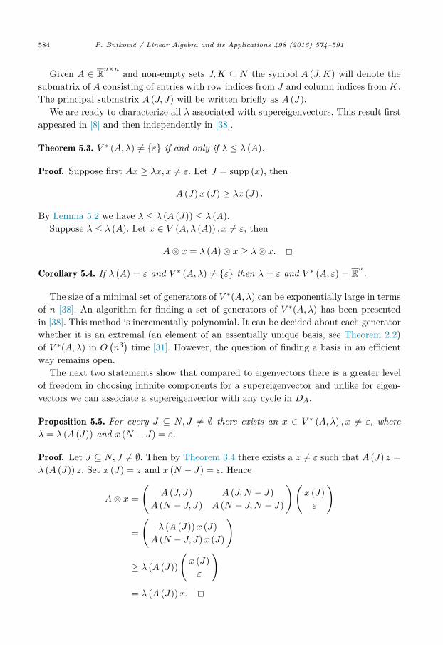
Given A ∈ Rn×n and non-empty sets J, K ⊆ N the symbol A (J,K) will denote the

submatrix of A consisting of entries with row indices from J and column indices from K. The principal submatrix A (J, J) will be written briefly as A (J).

We are ready to characterize all λ associated with supereigenvectors. This result first appeared in [8] and then independently in [38].

Theorem 5.3. V ∗ (A, λ) �= {ε} if and only if λ ≤ λ (A).

Proof. Suppose first Ax ≥ λx, x �= ε. Let J = supp (x), then

A (J)x (J) ≥ λx (J) .

By Lemma 5.2 we have λ ≤ λ (A (J)) ≤ λ (A).Suppose λ ≤ λ (A). Let x ∈ V (A, λ (A)) , x �= ε, then

A⊗ x = λ (A) ⊗ x ≥ λ⊗ x. �Corollary 5.4. If λ (A) = ε and V ∗ (A, λ) �= {ε} then λ = ε and V ∗ (A, ε) = R

n.

The size of a minimal set of generators of V ∗(A, λ) can be exponentially large in terms of n [38]. An algorithm for finding a set of generators of V ∗(A, λ) has been presented in [38]. This method is incrementally polynomial. It can be decided about each generator whether it is an extremal (an element of an essentially unique basis, see Theorem 2.2) of V ∗(A, λ) in O

(n3) time [31]. However, the question of finding a basis in an efficient

way remains open.The next two statements show that compared to eigenvectors there is a greater level

of freedom in choosing infinite components for a supereigenvector and unlike for eigen-vectors we can associate a supereigenvector with any cycle in DA.

Proposition 5.5. For every J ⊆ N, J �= ∅ there exists an x ∈ V ∗ (A, λ) , x �= ε, where λ = λ (A (J)) and x (N − J) = ε.

Proof. Let J ⊆ N, J �= ∅. Then by Theorem 3.4 there exists a z �= ε such that A (J) z =λ (A (J)) z. Set x (J) = z and x (N − J) = ε. Hence

A⊗ x =(

A (J, J) A (J,N − J)A (N − J, J) A (N − J,N − J)

)(x (J)ε

)

=(

λ (A (J))x (J)A (N − J, J)x (J)

)

≥ λ (A (J))(x (J)ε

)= λ (A (J))x. �

P. Butkovič / Linear Algebra and its Applications 498 (2016) 574–591 585

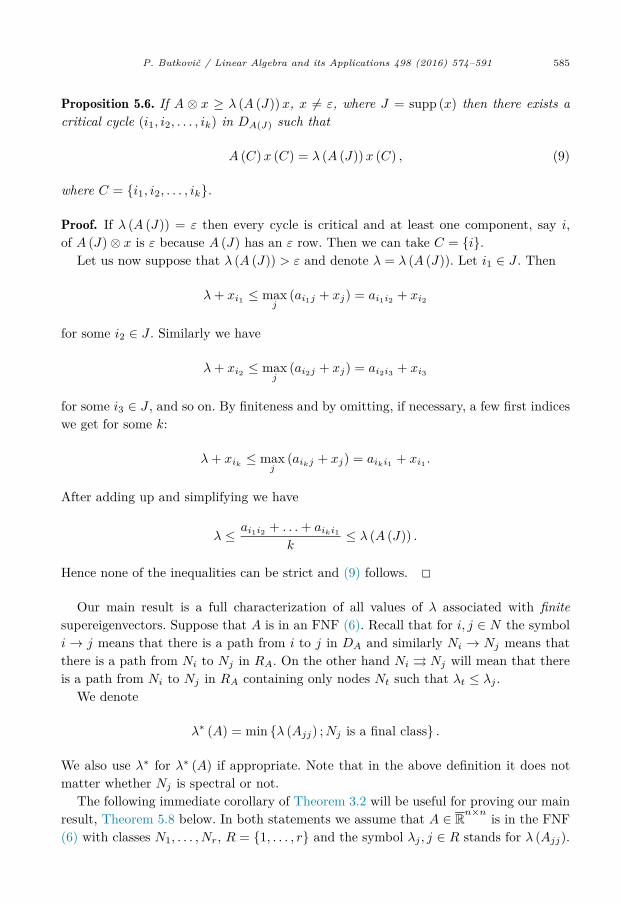
Proposition 5.6. If A ⊗ x ≥ λ (A (J))x, x �= ε, where J = supp (x) then there exists a critical cycle (i1, i2, . . . , ik) in DA(J) such that

A (C)x (C) = λ (A (J))x (C) , (9)

where C = {i1, i2, . . . , ik}.

Proof. If λ (A (J)) = ε then every cycle is critical and at least one component, say i, of A (J) ⊗ x is ε because A (J) has an ε row. Then we can take C = {i}.

Let us now suppose that λ (A (J)) > ε and denote λ = λ (A (J)). Let i1 ∈ J . Then

λ + xi1 ≤ maxj

(ai1j + xj) = ai1i2 + xi2

for some i2 ∈ J . Similarly we have

λ + xi2 ≤ maxj

(ai2j + xj) = ai2i3 + xi3

for some i3 ∈ J , and so on. By finiteness and by omitting, if necessary, a few first indices we get for some k:

λ + xik ≤ maxj

(aikj + xj) = aiki1 + xi1 .

After adding up and simplifying we have

λ ≤ ai1i2 + . . . + aiki1k

≤ λ (A (J)) .

Hence none of the inequalities can be strict and (9) follows. �Our main result is a full characterization of all values of λ associated with finite

supereigenvectors. Suppose that A is in an FNF (6). Recall that for i, j ∈ N the symbol i → j means that there is a path from i to j in DA and similarly Ni → Nj means that there is a path from Ni to Nj in RA. On the other hand Ni ⇒ Nj will mean that there is a path from Ni to Nj in RA containing only nodes Nt such that λt ≤ λj .

We denote

λ∗ (A) = min {λ (Ajj) ;Nj is a final class} .

We also use λ∗ for λ∗ (A) if appropriate. Note that in the above definition it does not matter whether Nj is spectral or not.

The following immediate corollary of Theorem 3.2 will be useful for proving our main result, Theorem 5.8 below. In both statements we assume that A ∈ R

n×n is in the FNF (6) with classes N1, . . . , Nr, R = {1, . . . , r} and the symbol λj , j ∈ R stands for λ (Ajj).

586 P. Butkovič / Linear Algebra and its Applications 498 (2016) 574–591

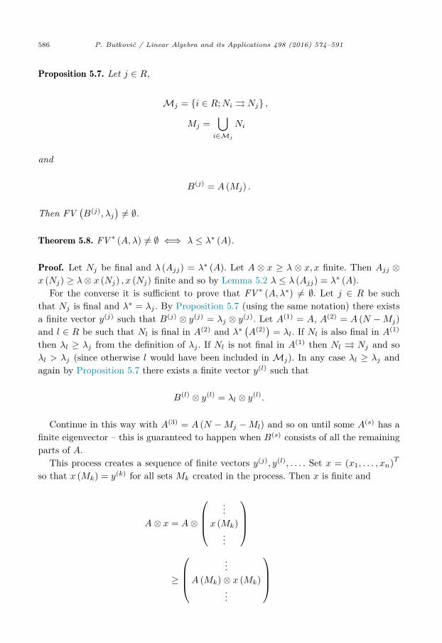
Proposition 5.7. Let j ∈ R,

Mj = {i ∈ R;Ni ⇒ Nj} ,

Mj =⋃

i∈Mj

Ni

and

B(j) = A (Mj) .

Then FV(B(j), λj

)�= ∅.

Theorem 5.8. FV ∗ (A, λ) �= ∅ ⇐⇒ λ ≤ λ∗ (A).

Proof. Let Nj be final and λ (Ajj) = λ∗ (A). Let A ⊗ x ≥ λ ⊗ x, x finite. Then Ajj ⊗x (Nj) ≥ λ ⊗ x (Nj) , x (Nj) finite and so by Lemma 5.2 λ ≤ λ (Ajj) = λ∗ (A).

For the converse it is sufficient to prove that FV ∗ (A, λ∗) �= ∅. Let j ∈ R be such that Nj is final and λ∗ = λj . By Proposition 5.7 (using the same notation) there exists a finite vector y(j) such that B(j) ⊗ y(j) = λj ⊗ y(j). Let A(1) = A, A(2) = A (N −Mj)and l ∈ R be such that Nl is final in A(2) and λ∗ (A(2)) = λl. If Nl is also final in A(1)

then λl ≥ λj from the definition of λj . If Nl is not final in A(1) then Nl ⇒ Nj and so λl > λj (since otherwise l would have been included in Mj). In any case λl ≥ λj and again by Proposition 5.7 there exists a finite vector y(l) such that

B(l) ⊗ y(l) = λl ⊗ y(l).

Continue in this way with A(3) = A (N −Mj −Ml) and so on until some A(s) has a finite eigenvector – this is guaranteed to happen when B(s) consists of all the remaining parts of A.

This process creates a sequence of finite vectors y(j), y(l), . . . . Set x = (x1, . . . , xn)T

so that x (Mk) = y(k) for all sets Mk created in the process. Then x is finite and

A⊗ x = A⊗

⎛⎜⎜⎝...

x (Mk)...

⎞⎟⎟⎠

≥

⎛⎜⎜⎝...

A (Mk) ⊗ x (Mk)...

⎞⎟⎟⎠

P. Butkovič / Linear Algebra and its Applications 498 (2016) 574–591 587

=

⎛⎜⎜⎝...

λk ⊗ x (Mk)...

⎞⎟⎟⎠

≥ λ∗ ⊗

⎛⎜⎜⎝...

x (Mk)...

⎞⎟⎟⎠ = λ∗ ⊗ x.

The last inequality follows because λk ≥ λ∗ for every k. �It is easily seen that the identification of Mj in Proposition 5.7 can be done in

polynomial time. Therefore the constructive proof above provides a method to find a non-trivial subset of a set of generators of finite supereigenvectors in polynomial time. If (in the notation of this proof) B is the n × t matrix (for some positive integer t) of the form ⎛⎜⎜⎜⎝

. . . ε ε

ε B(j)λj

ε

ε ε. . .

⎞⎟⎟⎟⎠then span+ (B) ⊆ FV ∗ (A, λ∗).

Remark 5.9. λ∗ (A) ranges over the whole discrete set {λ (Ajj) ; j ∈ R} and may be smaller or greater than λmin, or equal to λmin, for instance when

A =

⎛⎜⎝ α ε ε

0 2 ε

ε 0 1

⎞⎟⎠then for any α ∈ R we have λ (A) = max (2, α) , λmin = 1 and λ∗ (A) = α.

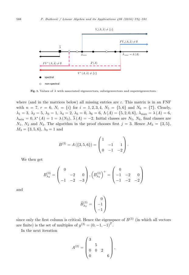
Fig. 1 shows a comparison of values of λ associated with general/finite eigenvectors, subeigenvectors and supereigenvectors.

We conclude with an example. Let A be the matrix⎛⎜⎜⎜⎜⎜⎜⎜⎜⎜⎝

35

10 0 0 2

0 0 −1 10 −1 −2

0 0 6

⎞⎟⎟⎟⎟⎟⎟⎟⎟⎟⎠,

588 P. Butkovič / Linear Algebra and its Applications 498 (2016) 574–591

Fig. 1. Values of λ with associated eigenvectors, subeigenvectors and supereigenvectors.

where (and in the matrices below) all missing entries are ε. This matrix is in an FNF with n = 7, r = 6, Ni = {i} for i = 1, 2, 3, 4, N5 = {5, 6} and N6 = {7}. Clearly, λ1 = 3, λ2 = 5, λ3 = 1, λ4 = 2, λ5 = 0, λ6 = 6, Λ (A) = {5, 2, 0, 6}, λmax = λ (A) = 6, λmin = 0, λ∗ (A) = 1 = λ (N3), λ (A) = −2. Initial classes are N5, N6, final classes are N1, N2 and N3. The algorithm in the proof chooses first j = 3. Hence M3 = {3, 5}, M3 = {3, 5, 6}, λ3 = 1 and

B(3) = A ({3, 5, 6}) =

⎛⎜⎝ 1−1 1

0 −1 −2

⎞⎟⎠ .

We then get

B(3)λ3

=

⎛⎜⎝ 0−2 0

−1 −2 −3

⎞⎟⎠ ,(B

(3)λ3

)+=

⎛⎜⎝ 0−1 −2 0−1 −2 −2

⎞⎟⎠and

B(3)λ3

=

⎛⎜⎝ 0−1−1

⎞⎟⎠since only the first column is critical. Hence the eigenspace of B(3) (in which all vectors are finite) is the set of multiples of y(3) = (0,−1,−1)T .

In the next iteration

A(2) =

⎛⎜⎜⎜⎝3

50 0 20 6

⎞⎟⎟⎟⎠ ,

P. Butkovič / Linear Algebra and its Applications 498 (2016) 574–591 589

l = 1, M1 = {1, 4} = M1, λ1 = 3 and

B(2) = A ({1, 4}) =(

30 2

).

Similarly as before the eigenspace of B(2) (in which all vectors are finite) is the set of multiples of y(2) = (0,−3)T .

In the next iteration

A(3) =(

56

),

l = 2, M2 = {2} = M2, λ2 = 5 and y(3) = (0)T .Finally,

A(4) =(

6),

l = 6, M7 = {7} = M6, λ6 = 6 and y(4) = (0)T .We conclude that finite supereigenvectors of A associated with λ exist if and only if

λ ≤ 1 and for any such λ we have span+ (B) ⊆ FV ∗ (A, λ), where

B =

⎛⎜⎜⎜⎜⎜⎜⎜⎜⎜⎝

00

0−3

−1−1

0

⎞⎟⎟⎟⎟⎟⎟⎟⎟⎟⎠.

We also observe that FV ∗ (A, λ) = R7 and V ∗(A, λ) = R

7 for all λ ≤ −2.

6. Conclusions

We have presented an overview of previously proved criteria for the existence of gen-eral and finite eigenvectors and subeigenvectors. We have then proved such criteria for general and finite supereigenvectors. A method for finding a non-trivial subset of a set of generators of finite supereigenvectors follows from the proof. However, efficient finding of a set of generators and a basis of the subspace of all general or finite supereigenvectors associated with a given λ ∈ R remains open.

Acknowledgements

This research was supported by EPSRC grant EP/J00829X/1.

590 P. Butkovič / Linear Algebra and its Applications 498 (2016) 574–591

References

[1] M. Akian, S. Gaubert, C. Walsh, Discrete max-plus spectral theory, in: G.L. Litvinov, V.P. Maslov (Eds.), Idempotent Mathematics and Mathematical Physics, in: Contemp. Math., vol. 377, AMS, 2005, pp. 53–77.

[2] F.L. Baccelli, G. Cohen, G.-J. Olsder, J.-P. Quadrat, Synchronization and Linearity, John Wiley, Chichester, New York, 1992.

[3] R.B. Bapat, D. Stanford, P. van den Driessche, The eigenproblem in max algebra, DMS-631-IR, University of Victoria, British Columbia, 1993.

[4] C.A. Brackley, D. Broomhead, M.C. Romano, M. Thiel, A max-plus model of ribosome dynamics during mRNA translation, J. Theoret. Biol. 303 (2012) 128–140.

[5] P. Butkovic, Max-algebra: the linear algebra of combinatorics?, Linear Algebra Appl. 367 (2003) 313–335.

[6] P. Butkovic, Finding a bounded mixed-integer solution to a system of dual inequalities, Oper. Res. Lett. 36 (2008) 623–627.

[7] P. Butkovic, Max-Linear Systems: Theory and Algorithms, Springer Monogr. Math., Springer-Verlag, London, 2010.

[8] P. Butkovic, Supereigenvectors, preprint, School of Mathematics, University of Birmingham, 2012/3.[9] P. Butkovic, R.A. Cuninghame-Green, S. Gaubert, Reducible spectral theory with applications to

the robustness of matrices in max-algebra, SIAM J. Matrix Anal. Appl. 31 (3) (2009) 1412–1431.[10] P. Butkovic, H. Schneider, Applications of max-algebra to diagonal scaling of matrices, Electron. J.

Linear Algebra 13 (2005) 262–273.[11] P. Butkovic, H. Schneider, S. Sergeev, Generators, extremals and bases of max cones, Linear Algebra

Appl. 421 (2007) 394–406.[12] P. Butkovic, H. Schneider, S. Sergeev, Recognizing weakly stable matrices, SIAM J. Control Optim.

50 (5) (2012) 3029–3051.[13] B.A. Carré, An algebra for network routing problems, J. Inst. Math. Appl. 7 (1971) 273–294.[14] G. Cohen, D. Dubois, J.-P. Quadrat, M. Viot, A linear-system-theoretic view of discrete-event

processes and its use for performance evaluation in manufacturing, IEEE Trans. Automat. Control AC-30 (3) (1985).

[15] R.A. Cuninghame-Green, Process synchronisation in a steelworks – a problem of feasibility, in: Banbury, Maitland (Eds.), Proc. 2nd Int. Conf. on Operational Research, English University Press, 1960, pp. 323–328.

[16] R.A. Cuninghame-Green, Describing industrial processes with interference and approximating their steady-state behaviour, Oper. Res. Quart. 13 (1962) 95–100.

[17] R.A. Cuninghame-Green, Minimax Algebra, Lecture Notes in Econom. and Math. Systems, vol. 166, Springer, Berlin, 1979.

[18] R.A. Cuninghame-Green, Minimax Algebra and Applications, Adv. Imaging Electron Phys., vol. 90, Academic Press, New York, 1995, pp. 1–121.

[19] L. Elsner, P. van den Driessche, On the power method in max algebra, in: Special Issue Dedicated to Hans Schneider, Madison, WI, 1998, Linear Algebra Appl. 302/303 (1999) 17–32.

[20] S. Gaubert, Théorie des systèmes linéaires dans les dioïdes, Thèse, Ecole des Mines de Paris, 1992.[21] J.S. Golan, Semirings and Their Applications, Kluwer Acad. Publ., Dordrecht, 1999.[22] M. Gondran, M. Minoux, Valeurs propres et vecteur propres dans les dioïdes et leur interprétation

en théorie des graphes, Bull. Direction Etudes Rech., Ser. C, Math. Inform. 2 (1977) 25–41.[23] M. Gondran, M. Minoux, Linear algebra of dioïds: a survey of recent results, Ann. Discrete Math.

19 (1984) 147–164.[24] B. Heidergott, G.-J. Olsder, J. van der Woude, Max Plus at Work: Modeling and Analysis of

Synchronized Systems: A Course on Max-Plus Algebra, PUP, 2005.[25] L. Hogben, et al., Handbook of Linear Algebra, Discrete Math. Appl., vol. 39, Chapman and Hall,

2006.[26] M. Joswig, Tropical convex hull computations, in: G.L. Litvinov, S.N. Sergeev (Eds.), Proceedings

of the International Conference on Tropical and Idempotent Mathematics, in: Contemp. Math., vol. 495, AMS, 2009, pp. 193–212.

[27] R.M. Karp, A characterization of the minimum cycle mean in a digraph, Discrete Math. 23 (1978) 309–311.

[28] V.N. Kolokoltsov, V.P. Maslov, Idempotent Analysis and Its Applications, Kluwer Acad. Publ., Dordrecht, 1997.

P. Butkovič / Linear Algebra and its Applications 498 (2016) 574–591 591

[29] W.M. McEneaney, Max-Plus Methods for Nonlinear Control and Estimation, Systems Control Found. Appl., Birkhäuser, 2006.

[30] G. Mikhalkin, Tropical geometry and its application, in: Proceedings of the ICM, Madrid, 2006, pp. 827–852.

[31] S. Sergeev, Extremals of the supereigenvector cone in max algebra: a combinatorial description, Linear Algebra Appl. 479 (2015) 106–117.

[32] S. Sergeev, H. Schneider, P. Butkovic, On visualization scaling, subeigenvectors and Kleene stars in max algebra, Linear Algebra Appl. 431 (2009) 2395–2406.

[33] D. Speyer, B. Sturmfels, Tropical mathematics, Math. Mag. 82 (2009) 163–173.[34] B. Sturmfels, et al., On the tropical rank of a matrix, in: J.E. Goodman, J. Pach, E. Welzl (Eds.),

Discrete and Computational Geometry, in: Math. Sci. Res. Inst. Publ., vol. 52, Cambridge University Press, 2005, pp. 213–242.

[35] N.N. Vorobyov, Extremal algebra of positive matrices, Elektron. Datenverarb. Kybernet. 3 (1967) 39–71 (in Russian).

[36] E. Wagneur, Finitely generated moduloïds: the existence and unicity problem for bases, in: J.L. Lions, A. Bensoussan (Eds.), Analysis and Optimization of Systems, Antibes, 1988, in: Lecture Notes in Control and Inform. Sci., vol. 111, Springer, Berlin, 1988, pp. 966–976.

[37] E. Wagneur, Moduloïds and pseudomodules: 1. Dimension theory, Discrete Math. 98 (1991) 57–73.[38] X. Wang, H. Wang, The generators of the solution space for a system of inequalities, Linear Algebra

Appl. 459 (2014) 248–263.[39] K. Zimmermann, Extremální Algebra, vol. 46, Výzkumná publikace Ekonomicko-matematické lab-

oratoře při Ekonomickém ústavě ČSAV, Praha, 1976 (in Czech).