www.elsevier.nl/locate/jelechem

Journal of Electroanalytical Chemistry 478 (1999) 25–32

Limiting current in normal pulse polarography with reactantadsorption obeying the Langmuir and the Frumkin isotherms

N. Fatouros *, D. KrulicLaboratoire LI2C-Electrochimie, Uni6ersite Pierre et Marie Curie, 4 place Jussieu, 75252 Paris Cedex 05, France

Received 5 July 1999; received in revised form 27 September 1999; accepted 28 September 1999

Abstract

A dimensionless analysis for the limiting current in normal pulse polarography (NPP) with reactant adsorption obeying theLangmuir and the Frumkin isotherms is presented. Zone diagrams, calculated numerically with reference to limiting cases whichcan be approached by analytical expressions, allow the determination of the adsorption parameters. Conclusions concerning theinitial accumulation of the adsorbate at zero current, apply to other voltammetries. © 1999 Elsevier Science S.A. All rightsreserved.

Keywords: Normal pulse polarography; Adsorption; Langmuir and Frumkin isotherms

1. Introduction

Adsorption of an electroactive species on the work-ing electrode before the application of the potential orat potentials where the rate of the electrochemicalreaction is low, greatly influences the response ofvoltamperometric methods. A typical example is thelimiting current in normal pulse polarography (NPP)which was essentially studied in the cases of low andstrong adsorptions [1–5]. A more detailed bibliographyis given in Ref. [3].

In the present work, it is shown that, when theLangmuir and the Frumkin isotherms are used, theadsorption at zero current can be described with twodimensionless variables. This allows zone diagrams tobe drawn which completely characterize the limitingcurrent in NPP. This new approach also permits thedefinition of the domain of validity of Henry’s linearlaw which is often used because it can lead to literalsolutions [6].

2. Approach of the problem

We assume that the working electrode is plane, thediffusion is the limiting step and the adsorption at zerocurrent, during a certain time t1, obeys Frumkin’sisotherm which can be stated as:

KGmax

c(0, t) exp(gu)=u

1−u(1)

Gmax is the limiting quantity adsorbed in a monolayeron the electrode surface, c(0, t) is the concentration ofthe surface-active compound at the electrode � solutioninterface, and:

u=G/Gmax (2)

is the fractional coverage of the surface. It is assumedthat the adsorption constant K and the g factor in Eq.(1) remain constant in the interval [0, t1], even if a stepoccurs between the equilibrium potential (open circuit)and the imposed potential. A positive value for the g

factor in Eq. (1) must be considered for attraction ofadsorbed particles. The constant:

b=K/Gmax (3)

is also used in this work.At low degrees of coverage, Eq. (1) reduces to Hen-

ry’s linear law:* Corresponding author. Fax: +33-44-27-3834.E-mail address: nf@ccr.jussieu.fr (N. Fatouros)

0022-0728/99/$ - see front matter © 1999 Elsevier Science S.A. All rights reserved.PII: S 0 0 2 2 -0728 (99 )00409 -X

N. Fatouros, D. Krulic / Journal of Electroanalytical Chemistry 478 (1999) 25–3226

bc(0, t)=u (4)

In our analysis, the distributions of concentration asa function of the distance x from the electrode, c(x, t),and the values of c(0, t1) are taken into account.

Let:

C0=c(0, t1)/c* (5)

and:

c=pDtIlim/nFADc* (6)

c is the ratio of the limiting current in NPP withreactant adsorption, Ilim, over the limiting current in theabsence of adsorption. In the above expressions, c* isthe bulk concentration of the adsorbate, D its diffusioncoefficient, n the number of electrons involved in theelectrochemical reaction, F the Faraday constant andA is the surface area of the electrode. Finally, Dt is thedelay of sampling of the current after the application ofthe potential step which leads to Ilim

2.1. Henry’s isotherm

We recently published [4,5] the formal solution forany stepped polarography with reactant adsorptionobeying Henry’s isotherm. In this case, C0 is given by:

C0=1−F(1/Y) (7)

with:

Y=K/Dt1 (8)

The function F is defined here as:

F(u)=exp(u2)erfc(u) (9)

From equation (10) in Ref. [4], c can be put in theform:

c=C0−pt

YF�1

Y�

−t

Y2

& 1+t

1

F(u/Y)

1+t−udu

+' t

1+t+

pt

Y�

1−2p

arctan1t

�(10)

where t is defined as:

t=Dt/t1 (11)

The function F and the integral in Eq. (10) can becalculated as indicated in Ref. [4] with high accuracy(up to 9 significant figures [7]). Eq. (10) shows thatwhen t tends to 0, c approaches C0. Moreover, thefollowing limits hold:

limy�0

C0=1, limy�0

c=1

limy��

C0=0, limy��

c=Dt/t=t/(1+t) (12)

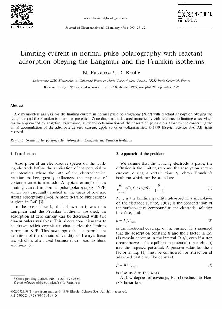
In Fig. 1, c is plotted as a function of log Y for t

equal to 0.02, 0.05 and 0.1. As Y decreases, the concen-tration profile at t1 near the electrode becomes moreand more horizontal and then c approaches C0. Thismeans that the limiting current in NPP with reactantadsorption can be equivalent to the limiting current inNPP without adsorption carried out with a bulk con-centration c*=c(0, t1). When tB0.1, the approxima-tion of c by C0 is valid at better than 5% for YB0.45.For Y=0.45, c is equal to 0.8.

2.2. Limiting cases independent of the adsorptionisotherm

When b�� (adsorption equilibrium almost unidi-rectional), up to a time t % where u becomes equal to 1,c(0, t) is nearly zero and then we have:

dG

dt=

c*D

pt(13)

From which:

u=G

Gmax

=2c*Dt

Gmaxp(14)

This relation was first considered for the study ofadsorption in polarography [8].

The dimensionless variable X is introduced:

X='t1

t %=

2c*Dt1

Gmaxp(15)

Two cases will be distinguished:1. tl5 t % or X51. In this case u(tl) is equal to X.

Moreover, at t\ tl after the application of the po-tential step, the diffusion still proceeds withc(0, t)#0. Consequently, Ilim, at time t is propor-tional to 1/t and c is equal to Dt/t. From thissimple reasoning, the same limiting value for c, as

Fig. 1. c calculated from Eq. (10), valid for Henry’s isotherm, isplotted as a function of log Y, for different values of t indicated onthe curves.

N. Fatouros, D. Krulic / Journal of Electroanalytical Chemistry 478 (1999) 25–32 27

Table 1Comparison of the values of C0 and c calculated both from Eqs. (7)and (10) and by numerical simulation a

C0 simY c (Eq. (10))C0 (Eq. (7)) c sim

10 11 1.000001.78×10−2 0.98996 0.98996 0.99017 0.99018

0.572221 0.611330.57242 0.611112.2545×10−6 0.14003 0.140032.2568×10−65×105

a For the numerical simulation, X=10−4.

pXYC exp(gu)/2=u/(1−u)

du/dT=pX((C/(L)/2

T\1:

C(0, T)=0, c=pt((C/(L)L=0

C(�, T)=1 (21)

This formulation shows that c is a function of X, Y,t and g. In particular, C(0, 1)=c(0, tl)/c* C0 obvi-ously depends on X, Y and g. Moreover, Henry’sequation holds when X�0 and Eq. (18) when Y��whatever g.

2.4. Numerical simulation

The diffusion equation is solved by the explicit finitedifferences method. For all calculations, the same FOR-

TRAN program was used. The general form of theadsorption isotherm (Eq. (1)) was introduced in calcu-lations. At each step time, this equation was solvedusing a root-finding algorithm by bisection and falseposition. The conditions for the time and space steps, dtand dx, were dt=5×10−6 s and Ddt/dx2=0.495.

In Table 1, results obtained from Eqs. (7) and (10)are compared with those of the numerical integration.It appears that, under the conditions used for thecalculations, the numerical integration is precise to atleast 4 significant figures.

2.5. Strong adsorption

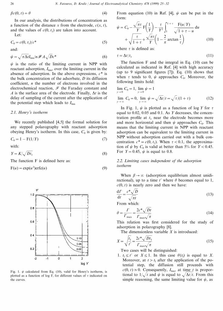
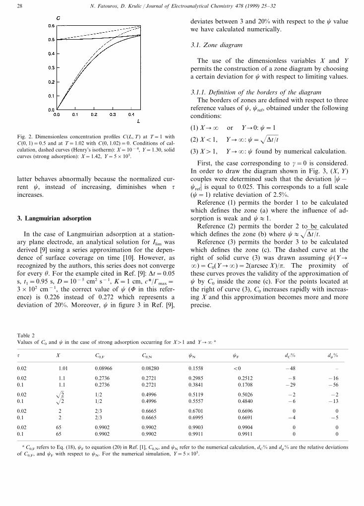
For a strong adsorption occurring when X\1 andY��, the concentration profile is more horizontalthan that in Henry’s domain having the same origin C0.For instance, when C0=0.5 the slope of the linear partof the concentration profile is 0.3%, whereas in thedomain of validity of Henry’s isotherm, it is 11%.

This appears clearly in Fig. 2 where the concentra-tion profiles at T=1 and at T=1.02 are presented forX=10−4 (X�0), Y=1.30 (dashed curves) and forX=1.42, Y=5×105 (Y��) (solid curves).

In Table 2, values of C0 and c for different values ofX are presented. Each time, c is calculated for twovalues of t, 0.02 and 0.1. C0,F refers to Eq. (18), C0,N

and cN, to the numerical simulation performed withoutany preliminary assumption. Finally, cF refers to equa-tion (20) in Ref. [1]. In this table, dC% and dc%represent the relative deviations in percentage of C0,F

and cF with respect to cN This table shows that Eq.(18), derived assuming that c(0, t)=0 at t5 t %, is suffi-ciently accurate for X\1.01, that is for values of t %close to t1. Table 2 also shows that for X close to 1 thesubstitution of c by C0 leads to better results than theapproximate solution (20) in Ref. [1]. Moreover, the

that found using Henry’s isotherm, is recovered (seeEq. (12)).

2. t1\ t % or X\1. In this case, u(tl)=1 and the diffu-sion in the interval [t %, tl] fills the concentrationprofile hollowed up to t %. The concentration profilec(x, t1) and c can be calculated from the diffusionequation:

#c#t

=D#2c#x2 (16)

with the conditions:

c(x, t %)=c*erf(x/2Dt %) (a)

t %B t5 t1:(#c/#x)x=0=0 (b)

t\ t1:c(0, t)=0 (c)

c=I/Ilim= (pDDt/c*)(#c/#x)x=0 (d)

c(�, t)=c* (e) (17)

Under these conditions, an approximate solution forc was previously presented [1].

The solution for C0=c(0, t1)/c* is (see Appendix A):

C0=2p

arctan X2−1=2p

arcsec X (18)

2.3. Description of adsorption by means ofdimensionless parameters

Using the dimensionless quantities X and Y, intro-duced in Sections 2.1 and 2.2, the adsorption isotherm(Eq. (1)) can be written at t= t1:

p

2XYC0 exp(gu)=

u

1−u(19)

Moreover, setting T= t/t1=1+t, L=x/Dt1, C=c/c*, the problem, in general, can be formulated as:

#C#T

=#2C#L2 (20)

with:

C(L, 0)=1

0BT51, L=0:

N. Fatouros, D. Krulic / Journal of Electroanalytical Chemistry 478 (1999) 25–3228

Fig. 2. Dimensionless concentration profiles C(L, T) at T=1 withC(0, 1)=0.5 and at T=1.02 with C(0, 1.02)=0. Conditions of cal-culation, dashed curves (Henry’s isotherm): X=10−4, Y=1.30, solidcurves (strong adsorption): X=1.42, Y=5×105.

deviates between 3 and 20% with respect to the c valuewe have calculated numerically.

3.1. Zone diagram

The use of the dimensionless variables X and Ypermits the construction of a zone diagram by choosinga certain deviation for c with respect to limiting values.

3.1.1. Definition of the borders of the diagramThe borders of zones are defined with respect to three

reference values of c, cref, obtained under the followingconditions:

(1) X�� or Y�0: c=1

(2) XB1, Y��: c=Dt/t

(3) X\1, Y��: c found by numerical calculation.

First, the case corresponding to g=0 is considered.In order to draw the diagram shown in Fig. 3, (X, Y)couples were determined such that the deviation �c−cref� is equal to 0.025. This corresponds to a full scale(c=1) relative deviation of 2.5%.

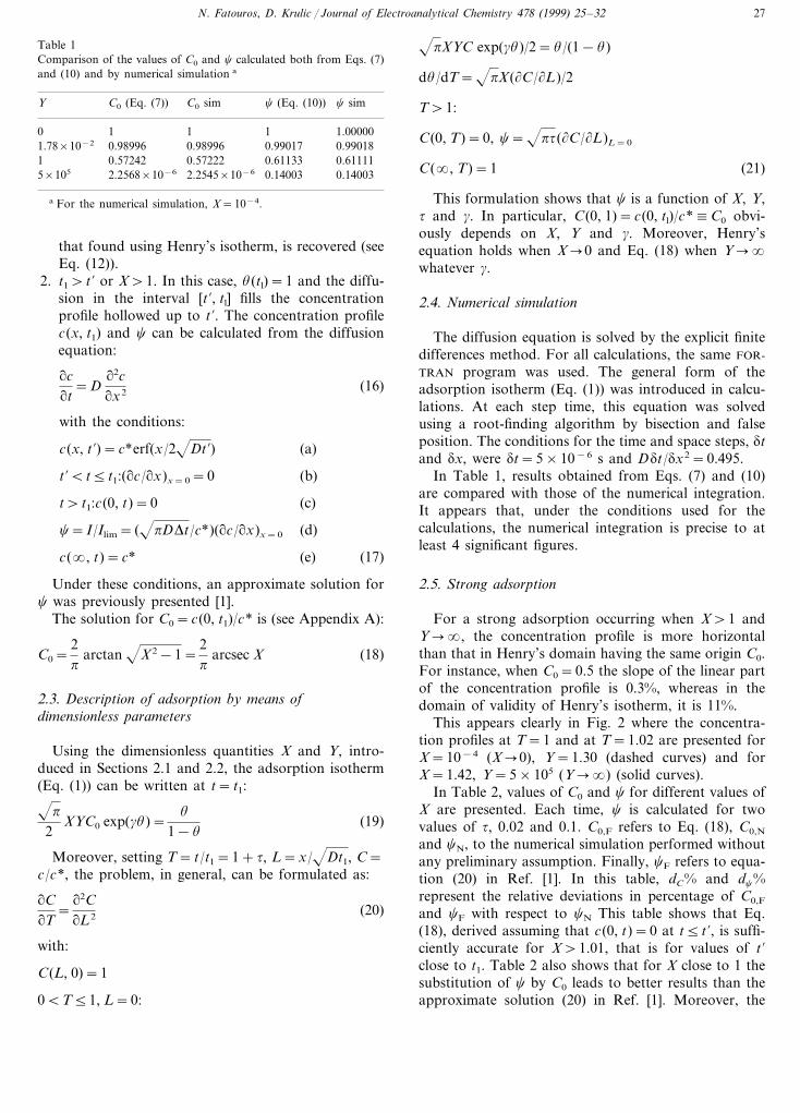
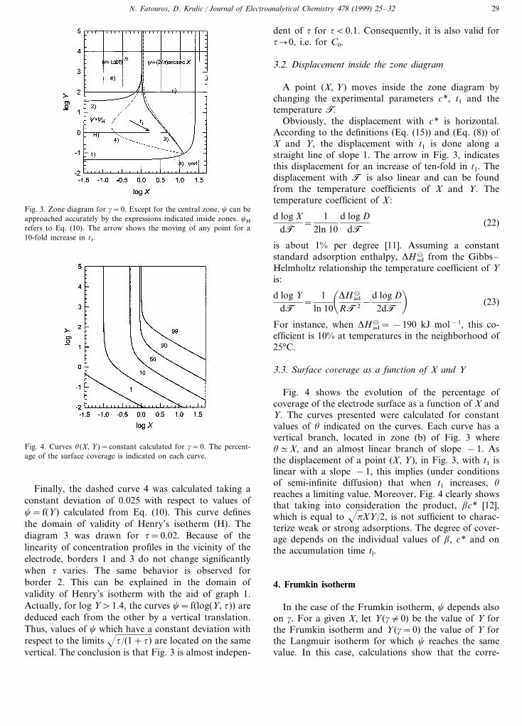
Reference (1) permits the border 1 to be calculatedwhich defines the zone (a) where the influence of ad-sorption is weak and c:1.

Reference (2) permits the border 2 to be calculatedwhich defines the zone (b) where c:Dt/t.

Reference (3) permits the border 3 to be calculatedwhich defines the zone (c). The dashed curve at theright of solid curve (3) was drawn assuming c(Y��)=C0(Y��)=2(arcsec X)/p. The proximity ofthese curves proves the validity of the approximation ofc by C0 inside the zone (c). For the points located atthe right of curve (3), C0 increases rapidly with increas-ing X and this approximation becomes more and moreprecise.

latter behaves abnormally because the normalized cur-rent c, instead of increasing, diminishes when t

increases.

3. Langmuirian adsorption

In the case of Langmuirian adsorption at a station-ary plane electrode, an analytical solution for Ilim wasderived [9] using a series approximation for the depen-dence of surface coverage on time [10]. However, asrecognized by the authors, this series does not convergefor every u. For the example cited in Ref. [9]: Dt=0.05s, t1=0.95 s, D=10−5 cm2 s−1, K=1 cm, c*/Gmax=3×102 cm−1, the correct value of c (F in this refer-ence) is 0.226 instead of 0.272 which represents adeviation of 20%. Moreover, c in figure 3 in Ref. [9],

Table 2Values of C0 and c in the case of strong adsorption occurring for X\1 and Y�� a

C0,NC0,Ft X dc%dC%cFcN

1.01 0.08966 0.082800.02 0.1558 B0 −48 –

1.1 −160.02 −80.2736 0.25120.29850.27211.10.1 −290.1708 −560.38410.27210.2736

1/2 0.4996 0.5119 0.5026 −20.02 −221/2 0.4996 0.5557 0.4840 −60.1 −132

00.66960.67010.6665 02/320.022/3 0.6665 0.6995 0.66910.1 −42 −5

0.990265 00.02 00.99040.99030.9902000.99110.99110.99020.99020.1 65

a C0,F refers to Eq. (18), cF to equation (20) in Ref. [1], C0,N, and cN refer to the numerical calculation, dC% and dc% are the relative deviationsof C0,F, and cF with respect to cN. For the numerical simulation, Y=5×105.

N. Fatouros, D. Krulic / Journal of Electroanalytical Chemistry 478 (1999) 25–32 29

Fig. 3. Zone diagram for g=0. Except for the central zone, c can beapproached accurately by the expressions indicated inside zones. cH

refers to Eq. (10). The arrow shows the moving of any point for a10-fold increase in t1.

dent of t for tB0.1. Consequently, it is also valid fort�0, i.e. for C0.

3.2. Displacement inside the zone diagram

A point (X, Y) moves inside the zone diagram bychanging the experimental parameters c*, t1 and thetemperature T.

Obviously, the displacement with c* is horizontal.According to the definitions (Eq. (15)) and (Eq. (8)) ofX and Y, the displacement with t1 is done along astraight line of slope 1. The arrow in Fig. 3, indicatesthis displacement for an increase of ten-fold in t1. Thedisplacement with T is also linear and can be foundfrom the temperature coefficients of X and Y. Thetemperature coefficient of X :

d log XdT

=1

2ln 10d log D

dT(22)

is about 1% per degree [11]. Assuming a constantstandard adsorption enthalpy, DHad

� from the Gibbs–Helmholtz relationship the temperature coefficient of Yis:

d log YdT

=1

ln 10�DHad

�

RT2 −d log D2dT

�(23)

For instance, when DHad�= −190 kJ mol−1, this co-

efficient is 10% at temperatures in the neighborhood of25°C.

3.3. Surface co6erage as a function of X and Y

Fig. 4 shows the evolution of the percentage ofcoverage of the electrode surface as a function of X andY. The curves presented were calculated for constantvalues of u indicated on the curves. Each curve has avertical branch, located in zone (b) of Fig. 3 whereu#X, and an almost linear branch of slope −1. Asthe displacement of a point (X, Y), in Fig. 3, with t1 islinear with a slope −1, this implies (under conditionsof semi-infinite diffusion) that when t1 increases, u

reaches a limiting value. Moreover, Fig. 4 clearly showsthat taking into consideration the product, bc* [12],which is equal to pXY/2, is not sufficient to charac-terize weak or strong adsorptions. The degree of cover-age depends on the individual values of b, c* and onthe accumulation time tl.

4. Frumkin isotherm

In the case of the Frumkin isotherm, c depends alsoon g. For a given X, let Y(g"0) be the value of Y forthe Frumkin isotherm and Y(g=0) the value of Y forthe Langmuir isotherm for which c reaches the samevalue. In this case, calculations show that the corre-

Fig. 4. Curves u(X, Y)=constant calculated for g=0. The percent-age of the surface coverage is indicated on each curve.

Finally, the dashed curve 4 was calculated taking aconstant deviation of 0.025 with respect to values ofc= f(Y) calculated from Eq. (10). This curve definesthe domain of validity of Henry’s isotherm (H). Thediagram 3 was drawn for t=0.02. Because of thelinearity of concentration profiles in the vicinity of theelectrode, borders 1 and 3 do not change significantlywhen t varies. The same behavior is observed forborder 2. This can be explained in the domain ofvalidity of Henry’s isotherm with the aid of graph 1.Actually, for log Y\1.4, the curves c= f(log(Y, t)) arededuced each from the other by a vertical translation.Thus, values of c which have a constant deviation withrespect to the limits t/(1+t) are located on the samevertical. The conclusion is that Fig. 3 is almost indepen-

N. Fatouros, D. Krulic / Journal of Electroanalytical Chemistry 478 (1999) 25–3230

Table 3C0, u and log Y calculated for g=2, 0 and −2 and for three different sets of values (X, c) a

u log Y Y(g)/Y(g=0) e−gu(g=0) d%g C0

(3a)2 0.0310 0.292 1.446 0.574 0.557 −2.9

0.292 1.687 1 1 00 0.03190.293 1.930 1.750.0328 1.79−2 2.6

(3b)0.370 −0.346 0.4512 0.4630.701 2.60.385 0 10.707 10 0

0.710−2 0.395 0.358 2.28 2.16 −5.3

(3c)0.497 −1.476 0.3630.974 0.3672 1.0

0.9740 0.502 −1.036 1 1 00.504−2 −0.5960.975 2.76 2.73 −1.0

a d% is the relative deviation of e−gu(g=0) with respect to Y(g)/Y(g=0). (3a) log X=−0.523, c=0.165. (3b) log X=0, c=0.725. (3c)log X=1.103, c=0.975.

sponding values of C0 are close to each other. The sameholds for the values of u. This behavior is evident in thedomain of strong adsorptions where u approaches 1and c tends to C0. Therefore, from Eq. (19), it followsthat:

Y(g)Y(g=0)

#exp(−gu) (24)

In Table 3, we present Y(g)/Y(g=0) and exp(−gu) forvalues of c corresponding to points (X, Y(g=0)) lo-cated in zone (b), in the central zone and in the bottomof zone (c) in Fig. 3. In each table, the extreme valuesfor the g factor usually admitted, 2 and −2 are consid-ered. The values of C0, and the deviation of exp(−gu)with respect to Y(g)/Y(g=0) (in general, less than 3%)are also presented. Eq. (24) allows us to obtain fromFigs. 3 and 4 established for g=0, the correspondingdiagrams for g"0. This transformation is performedby multiplying g by exp(−gu). For borders 1 and 3 inzone diagram 3, u is calculated by:

u=pXYC0

2+pXYC0

(25)

For border 1, C0 is equal to 0.975 and for border 3,C0= (2 arcsec X)/p+0.025. For border 2, u=X.

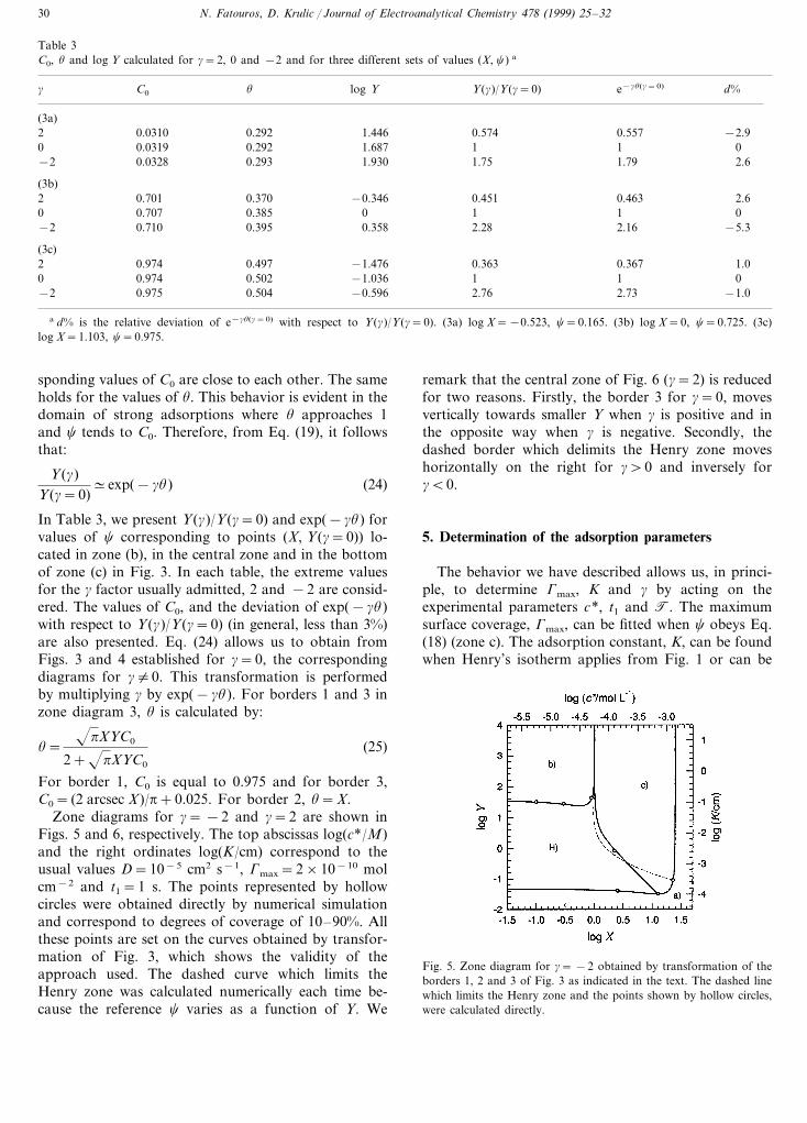
Zone diagrams for g= −2 and g=2 are shown inFigs. 5 and 6, respectively. The top abscissas log(c*/M)and the right ordinates log(K/cm) correspond to theusual values D=10−5 cm2 s−1, Gmax=2×10−10 molcm−2 and t1=1 s. The points represented by hollowcircles were obtained directly by numerical simulationand correspond to degrees of coverage of 10–90%. Allthese points are set on the curves obtained by transfor-mation of Fig. 3, which shows the validity of theapproach used. The dashed curve which limits theHenry zone was calculated numerically each time be-cause the reference c varies as a function of Y. We

remark that the central zone of Fig. 6 (g=2) is reducedfor two reasons. Firstly, the border 3 for g=0, movesvertically towards smaller Y when g is positive and inthe opposite way when g is negative. Secondly, thedashed border which delimits the Henry zone moveshorizontally on the right for g\0 and inversely forgB0.

5. Determination of the adsorption parameters

The behavior we have described allows us, in princi-ple, to determine Gmax, K and g by acting on theexperimental parameters c*, t1 and T. The maximumsurface coverage, Gmax, can be fitted when c obeys Eq.(18) (zone c). The adsorption constant, K, can be foundwhen Henry’s isotherm applies from Fig. 1 or can be

Fig. 5. Zone diagram for g= −2 obtained by transformation of theborders 1, 2 and 3 of Fig. 3 as indicated in the text. The dashed linewhich limits the Henry zone and the points shown by hollow circles,were calculated directly.

N. Fatouros, D. Krulic / Journal of Electroanalytical Chemistry 478 (1999) 25–32 31

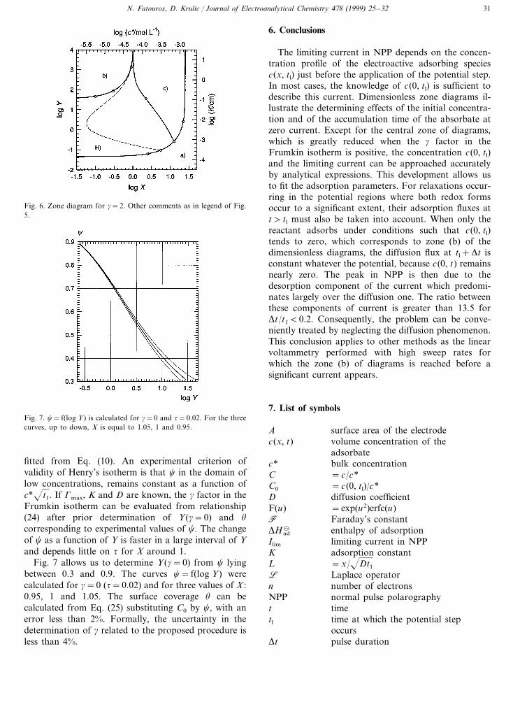
Fig. 6. Zone diagram for g=2. Other comments as in legend of Fig.5.

6. Conclusions

The limiting current in NPP depends on the concen-tration profile of the electroactive adsorbing speciesc(x, tl) just before the application of the potential step.In most cases, the knowledge of c(0, tl) is sufficient todescribe this current. Dimensionless zone diagrams il-lustrate the determining effects of the initial concentra-tion and of the accumulation time of the absorbate atzero current. Except for the central zone of diagrams,which is greatly reduced when the g factor in theFrumkin isotherm is positive, the concentration c(0, tl)and the limiting current can be approached accuratelyby analytical expressions. This development allows usto fit the adsorption parameters. For relaxations occur-ring in the potential regions where both redox formsoccur to a significant extent, their adsorption fluxes att\ tl must also be taken into account. When only thereactant adsorbs under conditions such that c(0, tl)tends to zero, which corresponds to zone (b) of thedimensionless diagrams, the diffusion flux at tl+Dt isconstant whatever the potential, because c(0, t) remainsnearly zero. The peak in NPP is then due to thedesorption component of the current which predomi-nates largely over the diffusion one. The ratio betweenthese components of current is greater than 13.5 forDt/t1B0.2. Consequently, the problem can be conve-niently treated by neglecting the diffusion phenomenon.This conclusion applies to other methods as the linearvoltammetry performed with high sweep rates forwhich the zone (b) of diagrams is reached before asignificant current appears.

7. List of symbols

A surface area of the electrodec(x, t) volume concentration of the

adsorbatebulk concentrationc*

C =c/c*C0 =c(0, tl)/c*D diffusion coefficientF(u) =exp(u2)erfc(u)

Faraday’s constantFDHad

� enthalpy of adsorptionIlim limiting current in NPP

adsorption constantKL =x/Dt1

L Laplace operatornumber of electronsn

NPP normal pulse polarographytimet

tl time at which the potential stepoccurspulse durationDt

Fig. 7. c= f(log Y) is calculated for g=0 and t=0.02. For the threecurves, up to down, X is equal to 1.05, 1 and 0.95.

fitted from Eq. (10). An experimental criterion ofvalidity of Henry’s isotherm is that c in the domain oflow concentrations, remains constant as a function ofc*t1. If Gmax, K and D are known, the g factor in theFrumkin isotherm can be evaluated from relationship(24) after prior determination of Y(g=0) and u

corresponding to experimental values of c. The changeof c as a function of Y is faster in a large interval of Yand depends little on t for X around 1.

Fig. 7 allows us to determine Y(g=0) from c lyingbetween 0.3 and 0.9. The curves c= f(log Y) werecalculated for g=0 (t=0.02) and for three values of X :0.95, 1 and 1.05. The surface coverage u can becalculated from Eq. (25) substituting C0 by c, with anerror less than 2%. Formally, the uncertainty in thedetermination of g related to the proposed procedure isless than 4%.

N. Fatouros, D. Krulic / Journal of Electroanalytical Chemistry 478 (1999) 25–3232

time for which u=1t %= t/tlTtemperature, Kelvin scaleT

x distance coordinate=t1/t %X=K/Dt1Y

Greek lettersb =K/Gmax

g interaction factor in the Frumkinisotherm

Gmax maximum surface concentration ofadsorbate

u surface fractional coveraget =Dt/t1

=I/Ilimc

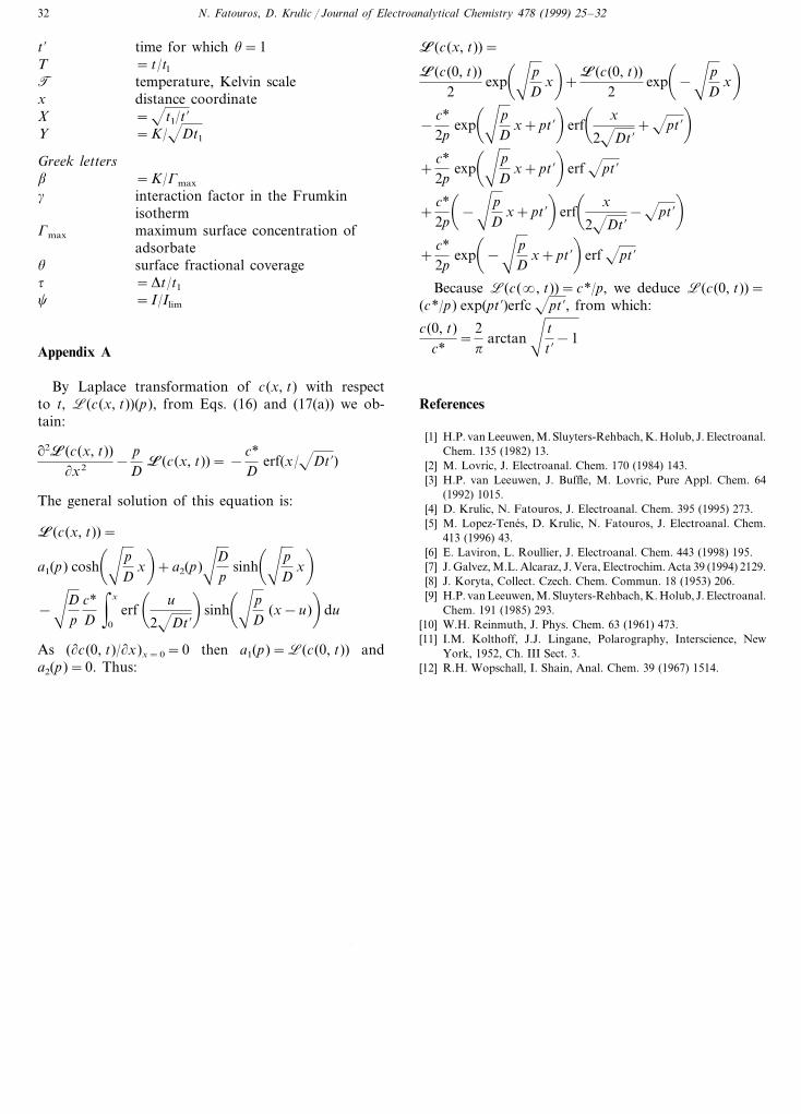
Appendix A

By Laplace transformation of c(x, t) with respectto t, L(c(x, t))(p), from Eqs. (16) and (17(a)) we ob-tain:

#2L(c(x, t))(x2 −

pD

L(c(x, t))= −c*D

erf(x/Dt %)

The general solution of this equation is:

L(c(x, t))=

a1(p) cosh�'p

Dx�

+a2(p)'D

psinh

�'pD

x�

−'D

pc*D

& x

0

erf� u

2Dt %

�sinh

�'pD

(x−u)�

du

As ((c(0, t)/(x)x=0=0 then a1(p)=L(c(0, t)) anda2(p)=0. Thus:

L(c(x, t))=

L(c(0, t))2

exp�'p

Dx�

+L(c(0, t))

2exp

�−'p

Dx�

−c*2p

exp�'p

Dx+pt %

�erf

� x

2Dt %+pt %

�+

c*2p

exp�'p

Dx+pt %

�erf pt %

+c*2p�

−'p

Dx+pt %

�erf

� x

2Dt %−pt %

�+

c*2p

exp�

−'p

Dx+pt %

�erf pt %

Because L(c(�, t))=c*/p, we deduce L(c(0, t))=(c*/p) exp(pt %)erfc pt %, from which:

c(0, t)c*

=2p

arctan' t

t %−1

References

[1] H.P. van Leeuwen, M. Sluyters-Rehbach, K. Holub, J. Electroanal.Chem. 135 (1982) 13.

[2] M. Lovric, J. Electroanal. Chem. 170 (1984) 143.[3] H.P. van Leeuwen, J. Buffle, M. Lovric, Pure Appl. Chem. 64

(1992) 1015.[4] D. Krulic, N. Fatouros, J. Electroanal. Chem. 395 (1995) 273.[5] M. Lopez-Tenes, D. Krulic, N. Fatouros, J. Electroanal. Chem.

413 (1996) 43.[6] E. Laviron, L. Roullier, J. Electroanal. Chem. 443 (1998) 195.[7] J. Galvez, M.L. Alcaraz, J. Vera, Electrochim. Acta 39 (1994) 2129.[8] J. Koryta, Collect. Czech. Chem. Commun. 18 (1953) 206.[9] H.P. van Leeuwen, M. Sluyters-Rehbach, K. Holub, J. Electroanal.

Chem. 191 (1985) 293.[10] W.H. Reinmuth, J. Phys. Chem. 63 (1961) 473.[11] I.M. Kolthoff, J.J. Lingane, Polarography, Interscience, New

York, 1952, Ch. III Sect. 3.[12] R.H. Wopschall, I. Shain, Anal. Chem. 39 (1967) 1514.

.