Embed Size (px)
Citation preview
Limited Dependent Variable Models I
Fall 2008
Environmental Econometrics (GR03) LDV Fall 2008 1 / 20
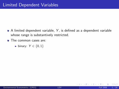
Limited Dependent Variables
A limited dependent variable, Y , is de�ned as a dependent variablewhose range is substantively restricted.
The common cases are:
binary: Y 2 f0, 1gmultinomial: Y 2 f0, 1, 2, ..., kginteger: Y 2 f0, 1, 2, ...gcensored: Y 2 fY � : Y � � 0g
Environmental Econometrics (GR03) LDV Fall 2008 2 / 20
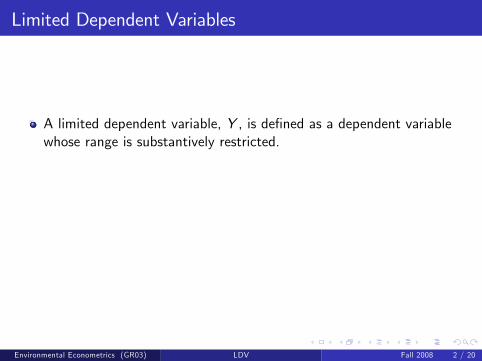
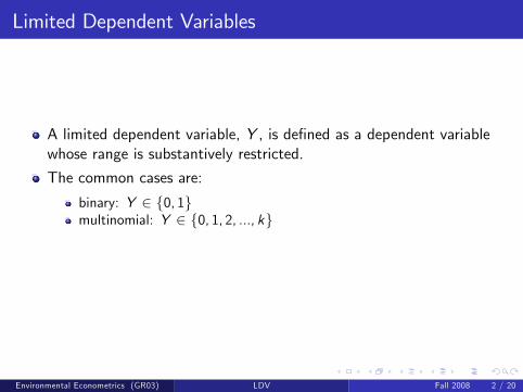
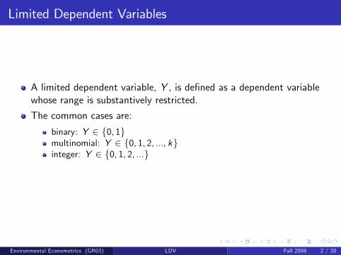
Limited Dependent Variables
A limited dependent variable, Y , is de�ned as a dependent variablewhose range is substantively restricted.
The common cases are:
binary: Y 2 f0, 1g
multinomial: Y 2 f0, 1, 2, ..., kginteger: Y 2 f0, 1, 2, ...gcensored: Y 2 fY � : Y � � 0g
Environmental Econometrics (GR03) LDV Fall 2008 2 / 20
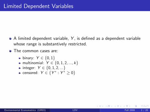
Limited Dependent Variables
A limited dependent variable, Y , is de�ned as a dependent variablewhose range is substantively restricted.
The common cases are:
binary: Y 2 f0, 1gmultinomial: Y 2 f0, 1, 2, ..., kg
integer: Y 2 f0, 1, 2, ...gcensored: Y 2 fY � : Y � � 0g
Environmental Econometrics (GR03) LDV Fall 2008 2 / 20
Limited Dependent Variables
A limited dependent variable, Y , is de�ned as a dependent variablewhose range is substantively restricted.
The common cases are:
binary: Y 2 f0, 1gmultinomial: Y 2 f0, 1, 2, ..., kginteger: Y 2 f0, 1, 2, ...g
censored: Y 2 fY � : Y � � 0g
Environmental Econometrics (GR03) LDV Fall 2008 2 / 20
Limited Dependent Variables
A limited dependent variable, Y , is de�ned as a dependent variablewhose range is substantively restricted.
The common cases are:
binary: Y 2 f0, 1gmultinomial: Y 2 f0, 1, 2, ..., kginteger: Y 2 f0, 1, 2, ...gcensored: Y 2 fY � : Y � � 0g
Environmental Econometrics (GR03) LDV Fall 2008 2 / 20
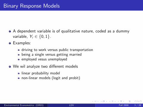
Binary Response Models
A dependent variable is of qualitative nature, coded as a dummyvariable, Yi 2 f0, 1g.Examples:
driving to work versus public transportationbeing a single versus getting marriedemployed vesus unemployed
We wil analyze two di¤erent models
linear probability modelnon-linear models (logit and probit)
Environmental Econometrics (GR03) LDV Fall 2008 3 / 20
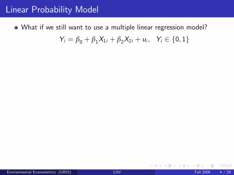
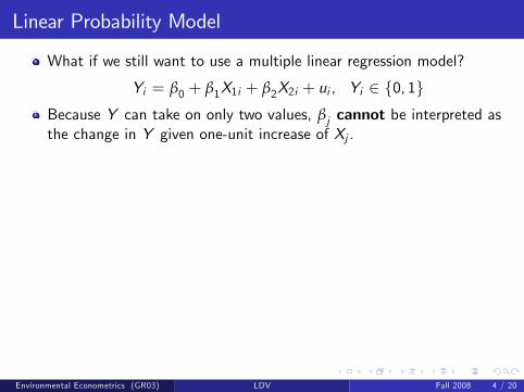
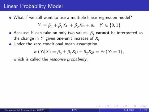
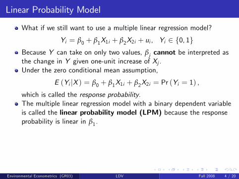
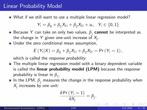
Linear Probability Model
What if we still want to use a multiple linear regression model?
Yi = β0 + β1X1i + β2X2i + ui , Yi 2 f0, 1g
Because Y can take on only two values, βj cannot be interpreted asthe change in Y given one-unit increase of Xj .Under the zero conditional mean assumption,
E (Yi jX ) = β0 + β1X1i + β2X2i = Pr (Yi = 1) ,
which is called the response probability.The multiple linear regression model with a binary dependent variableis called the linear probability model (LPM) because the responseprobability is linear in β1.In the LPM, βj measures the change in the response probability whenXj increases by one unit:
∂Pr (Yi = 1)∂Xj
= βj .
Environmental Econometrics (GR03) LDV Fall 2008 4 / 20
Linear Probability Model
What if we still want to use a multiple linear regression model?
Yi = β0 + β1X1i + β2X2i + ui , Yi 2 f0, 1gBecause Y can take on only two values, βj cannot be interpreted asthe change in Y given one-unit increase of Xj .
Under the zero conditional mean assumption,
E (Yi jX ) = β0 + β1X1i + β2X2i = Pr (Yi = 1) ,
which is called the response probability.The multiple linear regression model with a binary dependent variableis called the linear probability model (LPM) because the responseprobability is linear in β1.In the LPM, βj measures the change in the response probability whenXj increases by one unit:
∂Pr (Yi = 1)∂Xj
= βj .
Environmental Econometrics (GR03) LDV Fall 2008 4 / 20
Linear Probability Model
What if we still want to use a multiple linear regression model?
Yi = β0 + β1X1i + β2X2i + ui , Yi 2 f0, 1gBecause Y can take on only two values, βj cannot be interpreted asthe change in Y given one-unit increase of Xj .Under the zero conditional mean assumption,
E (Yi jX ) = β0 + β1X1i + β2X2i = Pr (Yi = 1) ,
which is called the response probability.
The multiple linear regression model with a binary dependent variableis called the linear probability model (LPM) because the responseprobability is linear in β1.In the LPM, βj measures the change in the response probability whenXj increases by one unit:
∂Pr (Yi = 1)∂Xj
= βj .
Environmental Econometrics (GR03) LDV Fall 2008 4 / 20
Linear Probability Model
What if we still want to use a multiple linear regression model?
Yi = β0 + β1X1i + β2X2i + ui , Yi 2 f0, 1gBecause Y can take on only two values, βj cannot be interpreted asthe change in Y given one-unit increase of Xj .Under the zero conditional mean assumption,
E (Yi jX ) = β0 + β1X1i + β2X2i = Pr (Yi = 1) ,
which is called the response probability.The multiple linear regression model with a binary dependent variableis called the linear probability model (LPM) because the responseprobability is linear in β1.
In the LPM, βj measures the change in the response probability whenXj increases by one unit:
∂Pr (Yi = 1)∂Xj
= βj .
Environmental Econometrics (GR03) LDV Fall 2008 4 / 20
Linear Probability Model
What if we still want to use a multiple linear regression model?
Yi = β0 + β1X1i + β2X2i + ui , Yi 2 f0, 1gBecause Y can take on only two values, βj cannot be interpreted asthe change in Y given one-unit increase of Xj .Under the zero conditional mean assumption,
E (Yi jX ) = β0 + β1X1i + β2X2i = Pr (Yi = 1) ,
which is called the response probability.The multiple linear regression model with a binary dependent variableis called the linear probability model (LPM) because the responseprobability is linear in β1.In the LPM, βj measures the change in the response probability whenXj increases by one unit:
∂Pr (Yi = 1)∂Xj
= βj .
Environmental Econometrics (GR03) LDV Fall 2008 4 / 20
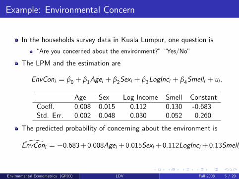
Example: Environmental Concern
In the households survey data in Kuala Lumpur, one question is
�Are you concerned about the environment?��Yes/No�
The LPM and the estimation are
EnvConi = β0 + β1Agei + β2Sexi + β3LogInci + β4Smelli + ui .
Age Sex Log Income Smell ConstantCoe¤. 0.008 0.015 0.112 0.130 -0.683Std. Err. 0.002 0.048 0.030 0.052 0.260
The predicted probability of concerning about the environment is
\EnvConi = �0.683+ 0.008Agei + 0.015Sexi + 0.112LogInci + 0.13Smelli .
Environmental Econometrics (GR03) LDV Fall 2008 5 / 20
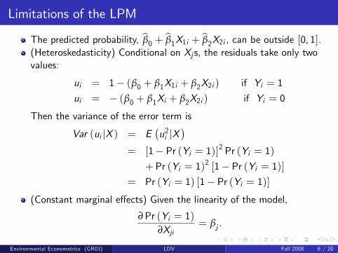
Limitations of the LPM
The predicted probability, bβ0 + bβ1X1i + bβ2X2i , can be outside [0, 1].(Heteroskedasticity) Conditional on Xj s, the residuals take only twovalues:
ui = 1� (β0 + β1X1i + β2X2i ) if Yi = 1
ui = � (β0 + β1Xi + β2X2i ) if Yi = 0
Then the variance of the error term is
Var (ui jX ) = E�u2i jX
�= [1� Pr (Yi = 1)]2 Pr (Yi = 1)
+Pr (Yi = 1)2 [1� Pr (Yi = 1)]
= Pr (Yi = 1) [1� Pr (Yi = 1)](Constant marginal e¤ects) Given the linearity of the model,
∂Pr (Yi = 1)∂Xji
= βj .
Environmental Econometrics (GR03) LDV Fall 2008 6 / 20
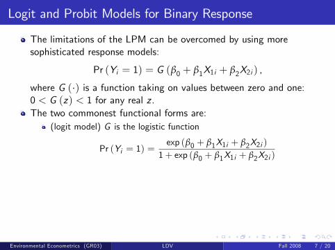
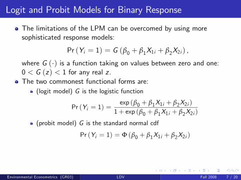
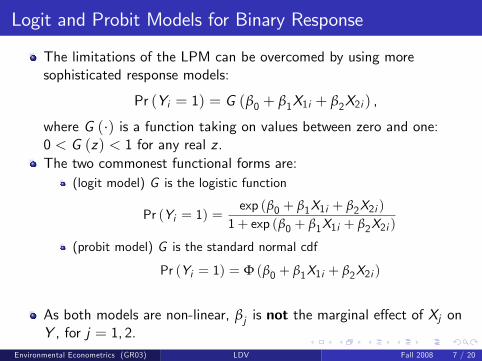
Logit and Probit Models for Binary Response
The limitations of the LPM can be overcomed by using moresophisticated response models:
Pr (Yi = 1) = G (β0 + β1X1i + β2X2i ) ,
where G (�) is a function taking on values between zero and one:0 < G (z) < 1 for any real z .
The two commonest functional forms are:
(logit model) G is the logistic function
Pr (Yi = 1) =exp (β0 + β1X1i + β2X2i )
1+ exp (β0 + β1X1i + β2X2i )
(probit model) G is the standard normal cdf
Pr (Yi = 1) = Φ (β0 + β1X1i + β2X2i )
As both models are non-linear, βj is not the marginal e¤ect of Xj onY , for j = 1, 2.
Environmental Econometrics (GR03) LDV Fall 2008 7 / 20
Logit and Probit Models for Binary Response
The limitations of the LPM can be overcomed by using moresophisticated response models:
Pr (Yi = 1) = G (β0 + β1X1i + β2X2i ) ,
where G (�) is a function taking on values between zero and one:0 < G (z) < 1 for any real z .The two commonest functional forms are:
(logit model) G is the logistic function
Pr (Yi = 1) =exp (β0 + β1X1i + β2X2i )
1+ exp (β0 + β1X1i + β2X2i )
(probit model) G is the standard normal cdf
Pr (Yi = 1) = Φ (β0 + β1X1i + β2X2i )
As both models are non-linear, βj is not the marginal e¤ect of Xj onY , for j = 1, 2.
Environmental Econometrics (GR03) LDV Fall 2008 7 / 20
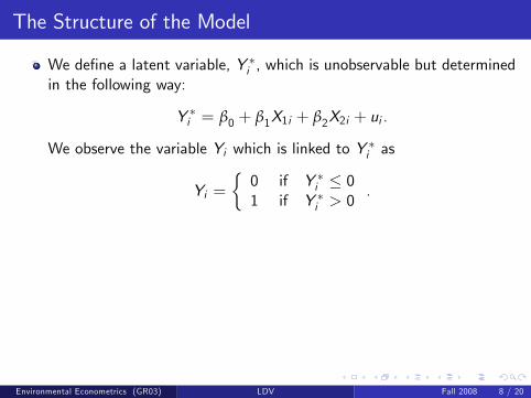
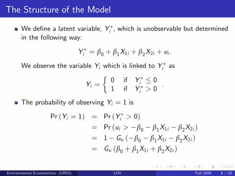
The Structure of the Model
We de�ne a latent variable, Y �i , which is unobservable but determinedin the following way:
Y �i = β0 + β1X1i + β2X2i + ui .
We observe the variable Yi which is linked to Y �i as
Yi =�01
if Y �i � 0if Y �i > 0
.
The probability of observing Yi = 1 is
Pr (Yi = 1) = Pr (Y �i > 0)
= Pr (ui > �β0 � β1X1i � β2X2i )
= 1� Gu (�β0 � β1X1i � β2X2i )
= Gu (β0 + β1X1i + β2X2i )
Environmental Econometrics (GR03) LDV Fall 2008 8 / 20
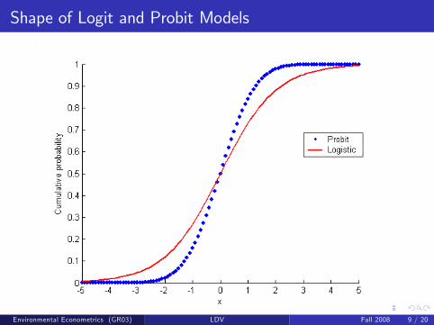
Shape of Logit and Probit Models
Environmental Econometrics (GR03) LDV Fall 2008 9 / 20
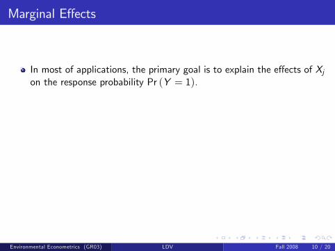
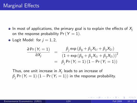
Marginal E¤ects
In most of applications, the primary goal is to explain the e¤ects of Xjon the response probability Pr (Y = 1).
Logit Model: for j = 1, 2,
∂Pr (Yi = 1)∂Xj
=βj exp (β0 + β1X1i + β2X2i )
(1+ exp (β0 + β1X1i + β2X2i ))2
= βj Pr (Yi = 1) (1� Pr (Yi = 1))
Thus, one unit increase in Xj leads to an increase ofβj Pr (Yi = 1) (1� Pr (Yi = 1)) in the response probability.
Environmental Econometrics (GR03) LDV Fall 2008 10 / 20
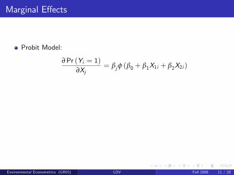
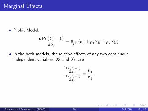
Marginal E¤ects
Probit Model:
∂Pr (Yi = 1)∂Xj
= βjφ (β0 + β1X1i + β2X2i )
In the both models, the relative e¤ects of any two continuousindependent variables, X1 and X2, are
∂Pr(Yi=1)∂X1
∂Pr(Yi=1)∂X2
=β1β2.
Environmental Econometrics (GR03) LDV Fall 2008 11 / 20
Marginal E¤ects
Probit Model:
∂Pr (Yi = 1)∂Xj
= βjφ (β0 + β1X1i + β2X2i )
In the both models, the relative e¤ects of any two continuousindependent variables, X1 and X2, are
∂Pr(Yi=1)∂X1
∂Pr(Yi=1)∂X2
=β1β2.
Environmental Econometrics (GR03) LDV Fall 2008 11 / 20
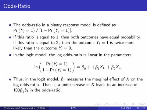
Odds-Ratio
The odds-ratio in a binary response model is de�ned asPr (Yi = 1) / [1� Pr (Yi = 1)].If this ratio is equal to 1, then both outcomes have equal probability.If this ratio is equal to 2 , then the outcome Yi = 1 is twice morelikely than the outcome Yi = 0.
In the logit model, the log odds-ratio is linear in the parameters:
ln�
Pr (Yi = 1)1� Pr (Yi = 1)
�= β0 ++β1X1i + β2X2i
Thus, in the logit model, β1 measures the marginal e¤ect of X on thelog odds-ratio. That is, a unit increase in X leads to an increase of100β1% in the odds-ratio.
Environmental Econometrics (GR03) LDV Fall 2008 12 / 20
Maximum Likelihood Estimation I
Both logit and probit models are non-linear models. We introduce anew estimation method, called the Maximum LikelihoodEstimation.Let f(Yi ,X1i , ...,Xki )gNi=1 denote a random sample from thepopulation distribution of Y conditional on X1, ...,Xk ,f (Y jX1, ...,Xk ; θ).The likelihood estimation requires the parametric assumption offunctional forms on f (Y jX1, ...,Xk ; θ) and we need to know the jointdistribution.
Environmental Econometrics (GR03) LDV Fall 2008 13 / 20
Maximum Likelihood Estimation II
Because of the random sampling assumption, the joint distribution off(Yi ,X1i , ...,Xki )gNi=1 is the product of the distributions:
(continuous variable) Πni=1f (Yi jX1i , ...,Xki ; θ)
(discrete variable) Πni=1 Pr (Yi jX1i , ...,Xki ; θ)
Then, the likelihood function is de�ned as
L�
θ; f(Yi ,X1i , ...,Xki )gNi=1�= Πn
i=1f (Yi jX1i , ...,Xki ; θ)
The maximum likelihood (ML) estimator of θ is the value of θ thatmaximizes the likelihood function.
Environmental Econometrics (GR03) LDV Fall 2008 14 / 20
Maximum Likelihood Estimation III
The ML principle says that, out of all the possible values for θ, thevalue that makes the likelihood of the observed data largest should bechosen.
Usually, it is more convenient to work with the log-likelihood function:
log L�
θ; f(Yi ,X1i , ...,Xki )gNi=1�=
n
∑i=1log f (Yi jX1i , ...,Xki ; θ) .
Because of the non-linear nature of the maximization problem, weusually cannot obtain an explict formula for ML estimators. Thus,one requires a numerical optimization.
Under very general conditions, the MLE is consistent, asymptoticallye¢ cient, and asymptotically normal.
Environmental Econometrics (GR03) LDV Fall 2008 15 / 20
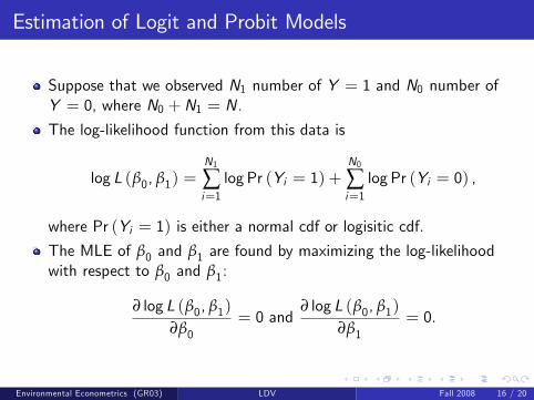
Estimation of Logit and Probit Models
Suppose that we observed N1 number of Y = 1 and N0 number ofY = 0, where N0 +N1 = N.
The log-likelihood function from this data is
log L (β0, β1) =N1
∑i=1log Pr (Yi = 1) +
N0
∑i=1log Pr (Yi = 0) ,
where Pr (Yi = 1) is either a normal cdf or logisitic cdf.
The MLE of β0 and β1 are found by maximizing the log-likelihoodwith respect to β0 and β1:
∂ log L (β0, β1)∂β0
= 0 and∂ log L (β0, β1)
∂β1= 0.
Environmental Econometrics (GR03) LDV Fall 2008 16 / 20
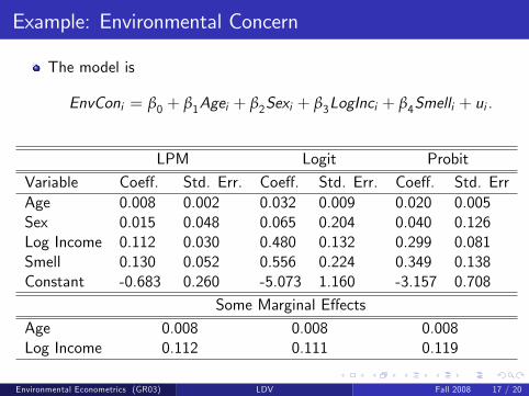
Example: Environmental Concern
The model is
EnvConi = β0 + β1Agei + β2Sexi + β3LogInci + β4Smelli + ui .
LPM Logit Probit
Variable Coe¤. Std. Err. Coe¤. Std. Err. Coe¤. Std. ErrAge 0.008 0.002 0.032 0.009 0.020 0.005Sex 0.015 0.048 0.065 0.204 0.040 0.126Log Income 0.112 0.030 0.480 0.132 0.299 0.081Smell 0.130 0.052 0.556 0.224 0.349 0.138Constant -0.683 0.260 -5.073 1.160 -3.157 0.708
Some Marginal E¤ects
Age 0.008 0.008 0.008Log Income 0.112 0.111 0.119
Environmental Econometrics (GR03) LDV Fall 2008 17 / 20
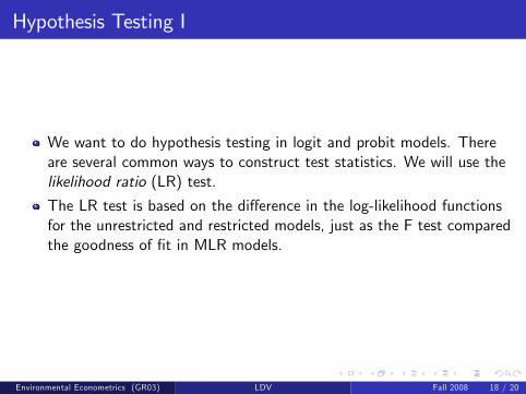
Hypothesis Testing I
We want to do hypothesis testing in logit and probit models. Thereare several common ways to construct test statistics. We will use thelikelihood ratio (LR) test.
The LR test is based on the di¤erence in the log-likelihood functionsfor the unrestricted and restricted models, just as the F test comparedthe goodness of �t in MLR models.
Environmental Econometrics (GR03) LDV Fall 2008 18 / 20
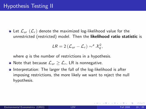
Hypothesis Testing II
Let Lur (Lr ) denote the maximized log-likelihood value for theunrestricted (restricted) model. Then the likelihood ratio statistic is
LR = 2 (Lur �Lr ) �a X 2q ,
where q is the number of restrictions in a hypothesis.
Note that because Lur � Lr , LR is nonnegative.Interpretation: The larger the fall of the log-likelihood is afterimposing restrictions, the more likely we want to reject the nullhypothesis.
Environmental Econometrics (GR03) LDV Fall 2008 19 / 20
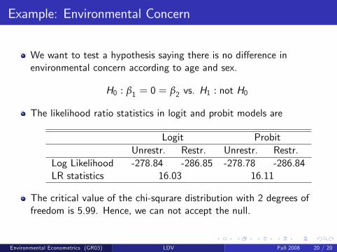
Example: Environmental Concern
We want to test a hypothesis saying there is no di¤erence inenvironmental concern according to age and sex.
H0 : β1 = 0 = β2 vs. H1 : not H0
The likelihood ratio statistics in logit and probit models are
Logit ProbitUnrestr. Restr. Unrestr. Restr.
Log Likelihood -278.84 -286.85 -278.78 -286.84LR statistics 16.03 16.11
The critical value of the chi-squrare distribution with 2 degrees offreedom is 5.99. Hence, we can not accept the null.
Environmental Econometrics (GR03) LDV Fall 2008 20 / 20