Embed Size (px)
Citation preview

ERRORS IN THE DEPENDENT VARIABLEOF QUANTILE REGRESSION MODELS
JERRY HAUSMAN, YE LUO, AND CHRISTOPHER PALMER
Abstract. The usual quantile regression estimator of Koenker and Bassett (1978) is biasedif there is an additive error term in the dependent variable. We analyze this problem as anerrors-in-variables problem where the dependent variable suffers from classical measurementerror and develop a sieve maximum-likelihood approach that is robust to left-hand side mea-surement error. After describing sufficient conditions for identification, we show that whenthe number of knots in the quantile grid is chosen to grow at an adequate speed, the sievemaximum-likelihood estimator is asymptotically normal. We verify our theoretical resultswith Monte Carlo simulations and illustrate our estimator with an application to the returnsto education highlighting important changes over time in the returns to education that havebeen obscured in previous work by measurement-error bias.
Keywords: Measurement Error, Quantile Regression, Functional Analysis
Date: April 2016.Hausman: MIT Department of Economics; [email protected]: Univeristy of Florida Department of Economics; [email protected]: Haas School of Business, University of California, Berkeley; [email protected] thank Victor Chernozhukov, Denis Chetverikov, Kirill Evdokimov, Brad Larsen, and Rosa Matzkin forhelpful discussions, as well as seminar participants at Cornell, Harvard, MIT, UCL, and UCLA. Haoyang Liu,Yuqi Song, and Jacob Ornelas provided outstanding research assistance.

ERRORS IN THE DEPENDENT VARIABLE OF QUANTILE REGRESSION MODELS 1
1. Introduction
Economists are aware of problems arising from errors-in-variables in regressors but generallyignore measurement error in the dependent variable. In this paper, we study the consequencesof measurement error in the dependent variable of conditional quantile models and propose amaximum likelihood approach to consistently estimate the distributional effects of covariatesin such a setting. Quantile regression (Koenker and Bassett, 1978) has become a very populartool for applied microeconomists to consider the effect of covariates on the distribution of thedependent variable. However, as left-hand side variables in microeconometrics often come fromself-reported survey data, the sensitivity of traditional quantile regression to LHS measurementerror poses a serious problem to the validity of results from the traditional quantile regressionestimator.
The errors-in-variables (EIV) problem has received significant attention in the linear model,including the well-known results that classical measurement error causes attenuation bias ifpresent in the regressors and has no effect on unbiasedness if present in the dependent variable.See Hausman (2001) for an overview. In general, the linear model results do not hold innonlinear models.1 We are particularly interested in the linear quantile regression setting.2
Hausman (2001) observes that EIV in the dependent variable in quantile regression modelsgenerally leads to significant bias, a result very different from the linear model intuition.
In general, EIV in the dependent variable can be viewed as a mixture model.3 We showthat under certain discontinuity assumptions, by choosing the growth speed of the number ofknots in the quantile grid, our estimator has fractional polynomial of n convergence speed andasymptotic normality. We suggest using the bootstrap for inference.
Intuitively, the estimated quantile regression line xi
b�(⌧) for quantile ⌧ may be far from theobserved y
i
because of LHS measurement error or because the unobserved conditional quantileui
of observation i is far from ⌧ . Our ML framework effectively estimates the likelihood that agiven quantile-specific residual ("
ij
⌘ yi
�xi
�(⌧j
)) is large because of measurement error ratherthan observation i’s unobserved conditional quantile u
i
being far away from ⌧j
. The estimate of
1Schennach (2008) establishes identification and a consistent nonparametric estimator when EIV exists in anexplanatory variable. Studies focusing on nonlinear models in which the left-hand side variable is measuredwith error include Hausman et. al (1998) and Cosslett (2004), who study probit and tobit models, respectively.2Carroll and Wei (2009) proposed an iterative estimator for the quantile regression when one of the regressorshas EIV.3A common feature of mixture models under a semiparametric or nonparametric framework is the ill-posedinverse problem, see Fan (1991). We face the ill-posed problem here, and our model specifications are linkedto the Fredholm integral equation of the first kind. The inverse of such integral equations is usually ill-posedeven if the integral kernel is positive definite. The key symptom of these model specifications is that the high-frequency signal of the objective we are interested in is wiped out, or at least shrunk, by the unknown noise ifits distribution is smooth. To uncover these signals is difficult and all feasible estimators have a lower speed ofconvergence compare to the usual
pn case. The convergence speed of our estimator relies on the decay speed of
the eigenvalues of the integral operator. We explain this technical problem in more detail in the related sectionof this paper.

2 HAUSMAN, LUO, AND PALMER
the joint distribution of the conditional quantile and the measurement error allows us to weightthe log likelihood contribution of observation i more in the estimation of �(⌧
j
) where they arelikely to have u
i
⇡ ⌧j
. In the case of Gaussian errors in variables, this estimator reduces toweighted least squares, with weights equal to the probability of observing the quantile-specificresidual for a given observation as a fraction of the total probability of the same observation’sresiduals across all quantiles.
An empirical example (extending Angrist et al., 2006) studies the heterogeneity of returnsto education across conditional quantiles of the wage distribution. We find that when wecorrect for likely measurement error in the self-reported wage data, we estimate considerablymore heterogeneity across the wage distribution in the returns to education. In particular, theeducation coefficient for the bottom of the wage distribution is lower than previously estimated,and the returns to education for latently high-wage individuals has been increasing over timeand is much higher than previously estimated. By 2000, the returns to education for the top ofthe conditional wage distribution are over three times larger than returns for any other segmentof the distribution.
The rest of the paper proceeds as follows. In Section 2, we introduce model specification andidentification conditions. In Section 3, we consider the MLE estimation method and analyzesits properties. In Section 4, we discuss sieve estimation. We present Monte Carlo simulationresults in Section 5, and Section 6 contains our empirical application. Section 7 concludes. TheAppendix contains an extension using the deconvolution method and additional proofs.
Notation: Define the domain of x as X . Define the space of y as Y. Denote a ^ b as theminimum of a and b, and denote a _ b as the larger of a and b. Let �!
d
be weak convergence(convergence in distribution), and �!
p
stands for convergence in probability. Let �!d
⇤ be weak
convergence in outer probability. Let f("|�) be the p.d.f of the EIV e parametrized by �.Assume the true parameters are �
0
(·) and �0
for the coefficient of the quantile model andparameter of the density function of the EIV. Let d
x
be the dimension of x. Let ⌃ be thedomain of �. Let d
�
be the dimension of parameter �. Define ||(�0,
�0
)|| :=p
||�0
||22
+ ||�0
||22
as the L2 norm of (�0,
�0
), where || · ||2
is the usual Euclidean norm. For �k
2 Rk, define||(�
k,
�0
)||2 :=p
||�k
||22
/k + ||�0
||22
.
2. Model and Identification
We consider the standard linear conditional quantile model, where the ⌧ th quantile of thedependent variable y⇤ is a linear function of x
Qy
⇤(⌧ |x) = x�(⌧).
However, we are interested in the situation where y⇤ is not directly observed, and we insteadobserve y where
y = y⇤ + "

ERRORS IN THE DEPENDENT VARIABLE OF QUANTILE REGRESSION MODELS 3
Figure 1. Check Function ⇢⌧
(z)
0
τ
1−τ
and " is a mean-zero, i.i.d error term independent from y⇤, x and ⌧ .Unlike the linear regression case where EIV in the left hand side variable does not matter
for consistency and asymptotic normality, EIV in the dependent variable can lead to severebias in quantile regression. More specifically, with ⇢
⌧
(z) denoting the check function (plottedin Figure 1)
⇢⌧
(z) = z(⌧ � 1(z < 0)),
the minimization problem in the usual quantile regression
�(⌧) 2 argmin
b
E[⇢⌧
(y � xb)], (2.1)
is generally no longer minimized at the true �0
(⌧) when EIV exists in the dependent variable.When there exists no EIV in the left-hand side variable, i.e. y⇤ is observed, the FOC is
E[x(⌧ � 1(y⇤ < x�(⌧)))] = 0, (2.2)
where the true �(⌧) is the solution to the above system of FOC conditions as shown by Koenkerand Bassett (1978). However, with left-hand side EIV, the FOC condition determining b�(⌧)becomes
E[x(⌧ � 1(y⇤ + " < x�(⌧)))] = 0. (2.3)
For ⌧ 6= 0.5, the presence of measurement error " will result in the FOC being satisfied ata different estimate of � than in equation (2.2) even in the case where " is symmetricallydistributed because of the asymmetry of the check function. In other words, in the minimization

4 HAUSMAN, LUO, AND PALMER
problem, observations for which y⇤ � x�(⌧) and should therefore get a weight of ⌧ may end upon the left-hand side of the check function, receiving a weight of (1 � ⌧) . Thus, equal-sizeddifferences on either side of zero do not cancel each other out.4
A straightforward analytical example below demonstrates the intuition behind the problemof left-hand errors in variables for estimators concerned with estimating the distributionalparameters. We then provide a simple Monte-Carlo simulation to show the degree of bias in asimple two-factor model with random disturbances on the dependent variable y.
Example 1. Consider the bivariate data-generating process
yi
= �0
(ui
) + �1
(ui
) · xi
+ "i
where xi
2 {0, 1}, the measurement error "i
is distributed N (0, 1), and the unobserved con-ditional quantile u
i
of observation i follows ui
⇠ U [0, 1]. Let the coefficient function �0
(⌧) =
�1
(⌧) = �
�1
(⌧), with �
�1
(·) representing the inverse CDF of the standard normal distribution.Because quantile regression estimates the conditional quantiles of y given x, in this simple set-ting, the estimated slope coefficient function is simply the difference in inverse CDFs for x = 1
and x = 0. For any quantile ⌧ , b�1
(⌧) = F�1
y|x=1
(⌧) � F�1
y|x=0
(⌧) where F (·) is the CDF of y.With no measurement error, the distribution y|x = 1 is N (0, 4) and the distribution of y|x = 0
is N (0, 1). In this case,b�1
(⌧) = (
p4�
p1)�
�1
(⌧) = �1
(⌧),
or the estimated coefficient equals the truth at each ⌧ . However, with non-zero measurementerror, y|x = 1 ⇠ N (0, 5) and y|x = 0 ⇠ N (0, 2). The estimated coefficient function undermeasurement error ˜�
1
(·) is
˜�1
(⌧) = (
p5�
p2)�
�1
(⌧),
which will not equal the truth for any quantile ⌧ 6= 0.5.
This example also illustrates the intuition offered by Hausman (2001) for compression biasfor bivariate quantile regression. For the median ⌧ = 0.5, because �
�1
(0.5) = 0, �(⌧) =
b�(⌧) =
˜�(⌧) = 0 such that the median is unbiased. For all other quantiles, however, sincep5 �
p2 < 1, the coefficient estimated under measurement error will be compressed towards
the true coefficient on the median regression �1
(0.5).
Example 2. We now consider a simulation exercise to illustrate the direction and magnitude ofmeasurement error bias in even simple quantile regression models. The data-generating process
4For median regression, ⌧ = .5 and so ⇢.5(·) is symmetric around zero. This means that if " is symmetrically
distributed and �(⌧) symmetrically distributed around ⌧ = .5 (as would be the case, for example, if �(⌧) werelinear in ⌧), the expectation in equation (2.3) holds for the true �0(⌧). However, for non-symmetric ", equation(2.3) is not satisfied at the true �0(⌧).

ERRORS IN THE DEPENDENT VARIABLE OF QUANTILE REGRESSION MODELS 5
Table 1. Monte-Carlo Results: Mean Bias
EIV Quantile (⌧)Parameter Distribution 0.1 0.25 0.5 0.75 0.9
�1
(⌧) = e⌧
" =0 0.006 0.003 0.002 0.000 -0.005" ⇠ N (0, 4) 0.196 0.155 0.031 -0.154 -0.272" ⇠ N (0, 16) 0.305 0.246 0.054 -0.219 -0.391
True parameter: 1.105 1.284 1.649 2.117 2.46
�2
(⌧) =p⌧
" =0 0.000 -0.003 -0.005 -0.006 -0.006" ⇠ N (0, 4) 0.161 0.068 -0.026 -0.088 -0.115" ⇠ N (0, 16) 0.219 0.101 -0.031 -0.128 -0.174
True parameter: 0.316 0.5 0.707 0.866 0.949Notes: Table reports mean bias (across 500 simulations) of slope coefficients estimated for each quantile⌧ from standard quantile regression of y on a constant, x1, and x2 where y = x1�1(⌧) + x2�2(⌧) + "and " is either zero (no measurement error case, i.e. y⇤ is observed) or " is distributed normally withvariance 4 or 16. The covariates x1 and x2 are i.i.d. draws from LN(0, 1). N = 1, 000.
for the Monte-Carlo results is
yi
= �0
(ui
) + x1i
�1
(ui
) + x2i
�2
(ui
) + "i
with the measurement error "i
again distributed as N (0,�2) and the unobserved conditionalquantile u
i
of observation i following ui
⇠ U [0, 1]. The coefficient function �(⌧) has components�0
(⌧) = 0, �1
(⌧) = exp(⌧), and �2
(⌧) =
p⌧ . The variables x
1
and x2
are drawn fromindependent lognormal distributions LN(0, 1). The number of observations is 1,000.
Table 1 presents Monte-Carlo results for three cases: when there is no measurement errorand when the variance of " equals 4 and 16. The simulation results show that under thepresence of measurement error, the quantile regression estimator is severely biased. Further-more, we find evidence of the attenuation-towards-the-median behavior posited by Hausman(2001), with quantiles above the median biased down and quantiles below the median upwardlybiased, understating the distributional heterogeneity in the �(·) function. For symmetricallydistributed EIV and uniformly distributed �(⌧), the median regression results appear unbiased.Comparing the mean bias when the variance of the measurement error increases from 4 to 16shows that the bias is increasing in the variance of the measurement error. Intuitively, theinformation of the functional parameter �(·) is decaying when the variance of the EIV becomeslarger.
2.1. Identification and Regularity Conditions. In the linear quantile model, it is assumedthat for any x 2 X , x�(⌧) is increasing in ⌧ . Suppose x
1
, ..., xd
x
are dx
-dimensional linearlyindependent vectors in int(X ). So Q
y
⇤(⌧ |x
i
) = xi
�(⌧) must be strictly increasing in ⌧ . Considerthe linear transformation of the model with matrix A = [x
1
, ..., xd
x
]
0:
Q⇤
y
(⌧ |x) = x�(⌧) = (xA�1
)(A�(⌧)). (2.4)
6 HAUSMAN, LUO, AND PALMER
Let ex = xA�1 and e�(⌧) = A�(⌧). The transformed model becomes
Q⇤
y
(⌧ |ex) = exe�(⌧), (2.5)
with every coefficient e�k
(⌧) being weakly increasing in ⌧ for k 2 {1, ..., dx
}. Therefore, WLOG,we can assume that the coefficients �(·) are increasing and refer to the set of functions {�
k
(·)}dxk=1
as co-monotonic functions. We therefore proceed assuming that �k
(·) is an increasing functionwhich has the properties of e�(⌧). All of the convergence and asymptotic results for e�
k
(⌧) holdfor the parameter �
k
after the inverse transform A�1.
Condition C1 (Properties of �(·)). We assume the following properties on the coefficient vectors�(⌧):
(1) �(⌧) is in the space M [B1
⇥B2
⇥B3
...⇥Bd
x
] where the functional space M is defined asthe collection of all functions f = (f
1
, ..., fd
x
) : [0, 1] ! [B1
⇥...⇥Bd
x
] with Bk
⇢ R beinga closed interval 8 k 2 {1, ..., d
x
} such that each entry fk
: [0, 1] ! Bk
is monotonicallyincreasing in ⌧ .
(2) Let Bk
= [lk
, uk
] so that lk
< �0k
(⌧) < uk
8 k 2 {1, ..., dx
} and ⌧ 2 [0, 1].(3) �
0
is a vector of C1 functions with derivative bounded from below by a positive constant.(4) The domain of the parameter � is a compact space ⌃ and the true value �
0
is in theinterior of ⌃.
Under assumption C1 it is easy to see that the parameter space ⇥ := M ⇥ ⌃ is compact.
Lemma 1. The space M [B1
⇥B2
⇥B3
...⇥Bk
] is a compact and complete space under Lp, forany p � 1.
Proof. See Appendix D.1. ⇤
Monotonicity of �k
(·) is important for identification because in the log-likelihood function,f(y|x) =
´1
0
f(y � x�(u)|�)du is invariant when the distribution of random variable �(u) isinvariant. The function �(·) is therefore unidentified if we do not impose further restrictions.Given the distribution of the random variable {�(u) |u 2 [0, 1]}, the vector of functions � :
[0, 1] ! B1
⇥B2
⇥ ...⇥Bd
x
is unique under the rearrangement if the functions {�k
(·)}dxk=1
areco-monotonic.
Condition C2 (Properties of x). We assume the following properties of the design matrix x:
(1) E[x0x] is non-singular.(2) The domain of x, denoted as X , is continuous on at least one dimension, i.e. there
exists k 2 {1, ..., dx
} such that for every feasible x�k
, there is a open set Xk
⇢ R suchthat (X
k,
x{�k}
) ⇢ X .(3) Without loss of generality, �
k
(0) � 0.

ERRORS IN THE DEPENDENT VARIABLE OF QUANTILE REGRESSION MODELS 7
Condition C3 (Properties of EIV). We assume the following properties of the measurementerror ":
(1) The probability function f("|�) is differentiable in �.(2) For all � 2 ⌃, there exists a uniform constant C > 0 such that E[| log f("|�)|] < C.(3) f(·) is non-zero all over the space R, and bounded from above.(4) E["] = 0.(5) Denote �(s|�) :=
´1
�1
exp(is")f("|�)d" as the characteristic function of ".(6) Assume for any �
1
and �2
in the domain of �, denoted as ⌃, there exists a neighborhoodof 0, such that �(s|�1)
�(s|�2)can be expanded as 1 +
P
1
k=2
ak
(is)k.
Denote ✓ := (�(·),�) 2 ⇥. For any ✓, define the expected log-likelihood function L(✓) asfollows:
L(✓) = E[log g(y|x, ✓)], (2.6)
where the conditional density function g(y|x, ✓) is defined as
g(y|x, ✓) =ˆ
1
0
f(y � x�(u)|�)du. (2.7)
Define the empirical likelihood as
Ln
(✓) = En
[log g(y|x, ✓)], (2.8)
The main identification results rely on the monotonicity of x�(⌧). The global identificationcondition is the following:
Condition C4 (Identification). There does not exist (�1
,�1
) 6= (�0
,�0
) in parameter space ⇥
such that g(y|x,�1
,�1
) = g(y|x,�0
,�0
) for all (x, y) with positive continuous density or positivemass.
Theorem 1 (Nonparametric Global Identification). Under condition C1-C3, for any �(·) andf(·) which generates the same density of y|x almost everywhere as the true function �
0
(·) andf0
(·), it must be that:�(⌧) = �
0
(⌧)
f(") = f0
(").
Proof. See Appendix D.1. ⇤
We also summarize the local identification condition as follows:
Lemma 2 (Local Identification). Define p(·) and �(·) as functions that measure the deviationof a given � or � from the truth: p(⌧) = �(⌧) � �
0
(⌧) and �(�) = � � �0
. Then there doesnot exist a function p(⌧) 2 L2
[0, 1] and � 2 Rd
� such that for almost all (x, y) with positive
8 HAUSMAN, LUO, AND PALMER
continuous density or positive massˆ1
0
f(y � x�(⌧)|�)xp(⌧)d⌧ =
ˆ1
0
�0f�
(y � x�(⌧))d⌧,
except that p(⌧) = 0 and � = 0.
Proof. See Appendix D.1. ⇤
Condition C5 (Stronger local identification for �). For any � 2 Sd
�
�1,
inf
p(⌧)2L
2[0,1]
✓ˆ1
0
fy
(y � x�(⌧)|�)xp(⌧)d⌧ �ˆ
1
0
�0f�
(y � x�(⌧))d⌧)2◆
> 0. (2.9)
3. Maximum Likelihood Estimator
3.1. Consistency. The ML estimator is defined as:
(
b�(·), b�) 2 arg max
(�(·),�)2⇥
En
[g(y|x,�(·),�)]. (3.1)
where g(·|·, ·, ·) is the conditional density of y given x and parameters, as defined in equation(2.7)
The following theorem states the consistency property of the ML estimator.
Lemma 3 (MLE Consistency). Under conditions C1-C3, the random coefficients �(·) and theparameter � that determines the distribution of " are identified in the parameter space ⇥. Themaximum-likelihood estimator
(
b�(·), b�) 2 arg max
(�(·),�)2⇥
En
log
ˆ1
0
f(y � x�(⌧)|�)d⌧�
exists and converges to the true parameter (�0
(·),�0
) under the L1 norm in the functionalspace M and Euclidean norm in ⌃ with probability approaching 1.
Proof. See Appendix D.2. ⇤
The identification theorem is a special version of a general MLE consistency theorem (Van derVaart, 2000). Two conditions play critical roles here: the co-monotonicity of the �(·) functionand the local continuity of at least one right-hand side variable. If we do not restrict theestimator in the family of monotone functions, then we will lose compactness of the parameterspace ⇥ and the consistency argument will fail.
3.2. Ill-posed Fredholm Integration of the First Kind. In the usual MLE setting withthe parameter being finite dimensional, the Fisher information matrix I is defined as:
I := E
@f
@✓
@f
@✓
0
�
.

ERRORS IN THE DEPENDENT VARIABLE OF QUANTILE REGRESSION MODELS 9
In our case, since the parameter is continuous, the informational kernel I(u, v) is defined as5
I(u, v)[p(v), �] = E
"
✓
f�(u)
g,g�
g
◆
0
✓ˆ1
0
fv
gp(v)dv +
g�
g
0
�
◆
#
. (3.2)
If we assume that we know the true �, i.e., � = 0, then the informational kernel becomes
I0
(u, v) := E[
@fu
g
@fu
g
0
].
By condition C5, the eigenvalue of I and I0
are both non-zero.Since E[X 0X] < 1, I
0
(u, v) is a compact (Hilbert-Schmidt) operator. From the RieszRepresentation Theorem, L(u, v) has countable eigenvalues �
1
� �2
� ... > 0 with 0 being theonly limit point of this sequence. It can be written as the following form:
I0
(·) =1
X
i=1
�i
h i
, ·i i
where i
is the system of orthogonal functional basis, i = 1, 2, . . .. For any function s(·),´1
0
I0
(u, v)h(v)dv = s(u) is called the Fredholm integral equation of the first kind. Thus, thefirst-order condition of the ML estimator is ill-posed. In Section (3.3) below, we establishconvergence rate results for the ML estimator using a deconvolution method.6
Although the estimation problem is ill-posed for the function �(·), the estimation problem isnot ill-posed for the finite dimensional parameter � given that E[g
�
g0�
] is non-singular. In theLemma below, we show that � converges to �
0
at rate 1/pn.
Lemma 4 (Estimation of �). If E[gsvg0sv] is positive definite and conditions C1-C5 hold, the MLestimator b� has the following property:
b� � �0
! Op
(n�
14). (3.3)
Proof. See Appendix D.2. ⇤
3.3. Bounds for the Maximum Likelihood Estimator. In this subsection, we use thedeconvolution method to establish bounds for the maximum likelihood estimator. Recall thatthe maximum likelihood estimator is the solution
(�,�) = argmax(�,�)2⇥
En
[log(g(y|x,�,�))]
5For notational convenience, we abbreviate @f(y�x�0(⌧)|�0)@�(⌧) as f
�(⌧), g(y|x,�0(⌧),�0) as g, and @g
@�
as g�
.6Kuhn (1990) shows that if the integral kernel is positive definite with smooth degree r, then the eigenvalue�i
is decaying with speed O(n�r�1). However, it is generally more difficult to obtain a lower bound for theeigenvalues. The decay speed of the eigenvalues of the information kernel is essential in obtaining convergencerate. From the Kuhn (1990) results, we see that the decay speed is linked with the degree of smoothness ofthe function f . The less smooth the function f is, the slower the decaying speed is. We show below that byassuming some discontinuity conditions, we can obtain a polynomial rate of convergence.

10 HAUSMAN, LUO, AND PALMER
Define �(s0
) = sup
|s|s0| 1
�
"
(s|�0)|. We use the following smoothness assumptions on the
distribution of " (see Evodokimov, 2010).
Condition C6 (Ordinary Smoothness (OS)). �(s0
) C(1 + |s0
|�).
Condition C7 (Super Smoothness (SS)). �(s0
) C1
(1 + |s0
|C2) exp(|s
0
|�/C3
).
The Laplace distribution L(0, b) satisfies the Ordinary Smoothness (OS) condition with � =
2. The Chi-2 Distribution �2
⌫
satisfies the OS condition with � =
⌫
2
. The Gamma Distribution�(⌫, ✓) satisfies the OS condition with � = ⌫. The Exponential Distribution satisfies conditionOS with � = 1. The Cauchy Distribution satisfies the Super Smoothness (SS) condition with� = 1. The Normal Distribution satisfies the SS condition with � = 2.
Lemma 5 (MLE Convergence Speed). Under assumptions C1-C5 and the results in Lemma 4,(1) if Ordinary Smoothness holds (C6), then the ML estimator of b� satisfies for all ⌧
|b�(⌧)� �0
(⌧)| - n�
12(1+�)
(2) if Super Smoothness holds (C7), then the ML estimator of b� satisfies for all ⌧
|b�(⌧)� �0
(⌧)| - log(n)�1� .
Proof. See Appendix D.2. ⇤
4. Sieve Estimation
In the last section we demonstrated that the maximum likelihood estimator restricted toparameter space ⇥ converges to the true parameter with probability approaching 1. However,the estimator still lives in a large space with �(·) being d
x
-dimensional co-monotone functionsand � being a finite dimensional parameter. Although theoretically such an estimator doesexist, in practice it is computationally infeasible to search for the likelihood maximizer withinthis large space. In this paper, we consider a spline estimator of �(·) to mimic the co-monotonefunctions �(·) for their computational advantages in calculating the sieve estimator. The es-timator below is easily adapted to the reader’s preferred estimator. For simplicity, we use apiecewise constant sieve space, which we define as follows.
Definition 1 (Sieve Space). Define ⇥
J
= ⌦
J
⇥ ⌃, where ⌦
J
stands for increasing piecewiseconstant functions on [0, 1] with J knots at
n
j
J
o
for j = 0, 1, ..., J � 1. In other words, for any
�(·) 2 ⌦
J
, �k
(·) is a piecewise constant function on intervals [
j
J
, j+1
J
) for j = 0, . . . , J � 1 andk = 1, . . . , d
x
.
We know that the L2 distance of the space ⇥
J
to the true parameter ✓0
satisfies d2
(✓0
,⇥J
) C
1J for some generic constant C.The sieve estimator is defined as follows:

ERRORS IN THE DEPENDENT VARIABLE OF QUANTILE REGRESSION MODELS 11
Definition 2 (Sieve Estimator).
(�J
(·),�) = arg max
✓2⇥
J
En
[log g(y|x,�,�)] (4.1)
Let d(✓1
, ✓2
)
2
:= E[
´R
(g(y|x,✓1)�g(y|x,✓2))2
g(y|x,✓0)dy] be a pseudo metric on the parameter space ⇥.
We know that d(✓, ✓0
) L(✓0
|✓0
)� L(✓|✓0
).Let || · ||
d
be a norm such that ||✓0
� ✓||d
Cd(✓0
, ✓). Our metric || · ||d
here is chosen to be:
||✓||2d
:= h✓, I(u, v)[✓]i . (4.2)
By Condition C4, || · ||d
is indeed a metric.For the sieve space ⇥
J
and any (⌦
J
,�) 2 ⇥
J
, define ˜I as the following matrix:
˜I := E
2
6
4
0
B
@
´ 1J
0
f⌧
d⌧,´ 2
J
1J
f⌧
d⌧, ...,´1
J�1J
f⌧
d⌧
g,g�
g
1
C
A
0
B
@
´ 1J
0
f⌧
d⌧,´ 2
J
1J
f⌧
d⌧, ...,´1
J�1J
f⌧
d⌧
g,g�
g
1
C
A
0
3
7
5
.
Again, by Condition C4, this matrix ˜I is non-singular. Furthermore, if a certain discontinuitycondition is assumed, the smallest eigenvalue of ˜I can be proved to be bounded away from somepolynomial of J .
Condition C8 (Discontinuity of f). Suppose there exists a positive integer � such that f 2C��1
(R), and the �th order derivative of f equals:
f (�)
(x) = h(x) + �(x� a), (4.3)
with h(x) being a bounded function and L1 Lipschitz except at a, and �(x � a) is a Dirac�-function at a.
Remark. The Laplace distribution satisfies the above assumption with � = 1. There is anintrinsic link between the above discontinuity condition and the tail property of the char-acteristic function stated as the (OS) condition. Because �
f
0(s) = is�
f
(s), we know that�f
(s) = 1
(is)
�
�f
(�)(s), while �f
(�)(s) = O(1) under the above assumption. Therefore, assump-tion C9 indicates that �
f
(s) := sup | 1
�
f
(s)
| C(1 + s�). In general, these results will hold aslong as the number of Dirac functions in f (�) are finite in (4.3).
The following Lemma establishes the decay speed of the minimum eigenvalue of ˜I.
Lemma 6. If the function f satisfies condition C8 with degree � > 0,(1) the minimum eigenvalue of ˜I, denoted as r(˜I), has the following property:
1
J�
- r(˜I).
(2) 1
J
�
- sup
✓2P
k
||✓||
d
||✓||

12 HAUSMAN, LUO, AND PALMER
Proof. See Appendix D.3. ⇤
The following Lemma establishes the consistency of the sieve estimator.
Lemma 7 (Sieve Estimator Consistency). If conditions C1-C6 and C9 hold, The sieve estima-tor defined in (4.1) is consistent.
Given the identification assumptions in the last section, if the problem is identified, thenthere exists a neighborhood · of ✓
0
, for any ✓ 2 �, ✓ 6= ✓0
, we have:
L(✓0
|✓0
)� L(✓|✓0
) � Ex
ˆY
(g(y|x, ✓0
)� g(y|x, ✓))2
g(y|x, ✓0
)
�
> 0. (4.4)
Proof. See Appendix D.3. ⇤
Unlike the usual sieve estimation problem, our problem is ill-posed with decaying eigen-value with speed J�. However, the curse of dimensionality is not at play because of theco-monotonicity: all entries of vector of functions �(·) are function of a single variable ⌧ . It istherefore possible to use sieve estimation to approximate the true functional parameter withthe number of intervals in the sieve J growing slower than
pn.
We summarize the tail property of f in the following condition:
Condition C 9 (Tail Property of f). Assume there exists a generic constant C such thatV ar
⇣
f
�
J
g0, g�g0
⌘
< C for any �J
(·) and � in a fixed neighborhood of (�0
(·), �0
).
Remark. The above condition is true for the Normal, Laplace, and Beta Distributions, amongothers.
Condition C10 (Eigenvector of ˜I). Suppose the smallest eigenvalue of ˜I, r(˜I) = c
J
J
�
. Suppose v
is a normalized eigenvector of r(˜I), and that J�↵ - min |vi
| for some fixed ↵ � 1
2
.
Theorem 2. Under conditions C1-C5 and C8-C10, the following results hold for the sieve-MLestimator:
(1) If the number of knots J satisfies the following growth condition:(a) J
2�+1p
n
! 0,
(b) J
�+r
p
n
! 1,
then ||✓ � ✓0
|| = Op
(
J
�
p
n
).(2) If condition 11 holds and the following growth conditions hold
(a) J
2�+1p
n
! 0
(b) J
�+r�↵
p
n
! 1,
then (a) for every j = 1, . . . , J , there exists a number µkjJ
, such that µ
kjJ
J
r
! 0, J
��↵
µ
kjJ
=
O(1), andµkjJ
(�k,J
(⌧j
)� �k,0
(⌧j
)) �!d
N (0, 1).
ERRORS IN THE DEPENDENT VARIABLE OF QUANTILE REGRESSION MODELS 13
and (b) for the parameter �, there exists a positive definite matrix V of dimension d�
⇥d�
such that the sieve estimator satisfies:pn(�
J
� �0
) ! N (0, V ).
Proof. See Appendix D.3. ⇤
Once we fix the number of interior points, we can use ML to estimate the sieve estimator.We discuss how to compute the sieve-ML estimator in the next section.
4.1. Inference via Bootstrap. In the last section we proved asymptotic normality for thesieve-ML estimator ✓ = (�(⌧),�). However, computing the convergence speed µ
kjJ
for �k,J
(⌧j
)
by explicit formula can be difficult in general. To conduct inference, we recommend usingnonparametric bootstrap. Define (xb
i
, ybi
) as a resampling of data (xi
, yi
) with replacement forbootstrap iteration b = 1, . . . B, and define the estimator
✓b = arg max
✓2⇥
J
Eb
n
[log g(ybi
|xbi
, ✓)], (4.5)
where Eb
n
denotes the operator of empirical average over resampled data for bootstrap iterationb. Then our preferred form of the nonparametric bootstrap is to construct the 95% ConfidenceInterval pointwise for each covariate k and quantile ⌧ from the variance dV ar(�
k
(⌧)) of each
vector of bootstrap coefficients�
�bk
(⌧)
B
b=1
as b�k
(⌧)± z1�↵/2
·q
dV ar(�k
(⌧)) where the criticalvalue z
1�↵/2
⇡ 1.96 for significance level of ↵ = .05.Chen and Pouzo (2013) establishes results in validity of the nonparametric bootstrap in
semiparametric models for a general functional of a parameter ✓. The Lemma below is animplementation of theorem (5.1) of Chen and Pouzo (2013), and establishes the asymptoticnormality of the bootstrap estimates that allows us, for example, to use their empirical varianceto construct bootstrapped confidence intervals.
Lemma 8 (Validity of the Bootstrap). Under condition C1-C6 and C9, choosing the number ofknots J according to the condition stated in Theorem 1, the bootstrap defined in equation (4.5)has the following property:
�bk,J
(⌧)� �k,J
(⌧)
µkjJ
⇤�!d
N (0, 1) (4.6)
Proof. See Appendix D.3. ⇤
4.2. Weighted Least Squares. Under normality assumption of the EIV term ", the max-imization of Q(·|✓) reduces to the minimization of a simple weighted least square problem.Suppose the disturbance " ⇠ N (0,�2). Then the maximization problem (4.1) becomes the

14 HAUSMAN, LUO, AND PALMER
following, with the parameter vector ✓ = [�(·),�]
max
✓
0Q(✓0|✓) := E
⇥
log(f(y � x�0(⌧))|✓0)(x, y, ✓)|✓⇤
(4.7)
= E"ˆ
1
⌧
f(y � x�(⌧)|�)´1
0
f(y � x�(u)|�)du
✓
�1
2
log(2⇡�02)� (y � x�0(⌧))2
2�02
◆
d⌧
#
.
It is easy to see from the above equation that the maximization problem of �0(·)|✓ is tominimize the sum of weighted least squares. As in standard normal MLE, the FOC for �0(·)does not depend on �02. The �02 is solved after all the �0(⌧) are solved from equation (4.7).Therefore, the estimand can be implemented with an EM algorithm that reduces to iterationon weighted least squares, which is both computationally tractable and easy to implement inpractice.
Given an initial estimate of a weighting matrix W , the weighted least squares estimates of� and � are
b�(⌧j
) = (X 0Wj
X)
�1X 0Wj
y
b� =
s
1
NJ
X
j
X
i
wij
b"2ij
where Wj
is the diagonal matrix formed from the jth column of W , which has elements wij
.Given estimates b"
j
= y �X b�(⌧j
) and b�, the weights wij
for observation i in the estimationof �(⌧
j
) are
wij
=
� (b"ij
/b�)1
J
P
j
� (b"ij
/b�)(4.8)
where �(·) is the pdf of a standard normal distribution J is the number of ⌧s in the sieve, e.g.J = 9 if the quantile grid is {⌧
j
} = {0.1, 0.2, ..., 0.9}.
5. Monte-Carlo Simulations
We examine the properties of our estimator empirically in Monte-Carlo simulations. Let thedata-generating process be
yi
= �0
(ui
) + x1i
�1
(ui
) + x2i
�2
(ui
) + "i
where n = 100, 000, the conditional quantile ui
of each individual is u ⇠ U [0, 1], and thecovariates are distributed as independent lognormal random variables, i.e. x
1i
, x2i
⇠ LN(0, 1).The coefficient vector is a function of the conditional quantile u
i
of individual i0
B
@
�0
(u)
�1
(u)
�2
(u)
1
C
A
=
0
B
@
1 + 2u� u2
1
2
exp(u)
u+ 1
1
C
A
.

ERRORS IN THE DEPENDENT VARIABLE OF QUANTILE REGRESSION MODELS 15
In our baseline scenario, we draw mean-zero measurement error " from a mixed normal distri-bution
"i
⇠
8
>
>
<
>
>
:
N (�3, 1) with probability 0.5
N (2, 1) with probability 0.25
N (4, 1) with probability 0.25
We also probe the robustness of the mixture specification by simulating measurement error fromalternative distributions and testing how well modeling the error distribution as a Gaussian mix-ture handles alternative scenarios to simulate real-world settings in which the econometriciandoes not know the true distribution of the residuals.
We use a gradient-based constrained optimizer to find the maximizer of the log-likelihoodfunction defined in Section 3. See Appendix A for a summary of the constraints we impose andanalytic characterizations of the log-likelihood gradients for a mixture of three normals. We usequantile regression coefficients for a ⌧ -grid of J = 9 knots as start values. For the start valuesof the distributional parameters, we place equal 1/3 weights on each mixture component, withunit variance and means -1, 0, and 1.
As discussed in Section 2.1, the likelihood function is invariant to a permutation of theparticular quantile labels. For example, the log-likelihood function defined by equations (2.6)and (2.7) would be exactly the same if �(⌧ = .2) were exchanged with �(⌧ = .5). Rearrangementhelps ensure that the final ordering is consistent with the assumption of x�(⌧) being monotonicin ⌧ and weakly reduces the L2 distance of the estimator b�(·) with the true parameter functional�(·). See Chernozhukov et al. (2009) for further discussion. Accordingly, we sort our estimatedcoefficient vectors by x̄b�(⌧) where x̄ is the mean of the design matrix across all observations.Given initial estimates ˜�(·), we take our final estimates for each simulation to be
n
b�(⌧j
)
o
for
j = 1, ..., J where b�(⌧j
) =
˜�(⌧r
) and r is the element of ˜�(·) corresponding to the jth smallestelement of the vector x̄˜�(·).
5.1. Simulation Results. In Figures 2 and 3, we plot the mean bias (across 500 MonteCarlo simulations) of quantile regression of y (generated with measurement error drawn from amixture of three normals) on a constant, x
1
, and x2
and contrast that with the mean bias of ourestimator using a sieve for �(·) consisting of 9 knots. Quantile regression is badly biased, withlower quantiles biased upwards towards the median-regression coefficients and upper quantilesbiased downwards towards the median-regression coefficients. While this pattern of bias towardsthe median evident in Table 2 still holds, the pattern in Figures 2 and 3 is nonmonotonic forquantiles below the median in the sense that the bias is actually greater for, e.g., ⌧ = 0.3 thanfor ⌧ = 0.1. Simulations reveal that the monotonic bias towards the median result seems torely on a symmetric error distribution. Regardless, the bias of the ML estimator is statisticallyindistinguishable from zero across quantiles of the conditional distribution of y given x, with anaverage mean bias across quantiles of 2% and 1% (for �
1
and �2
, respectively) and always less
16 HAUSMAN, LUO, AND PALMER
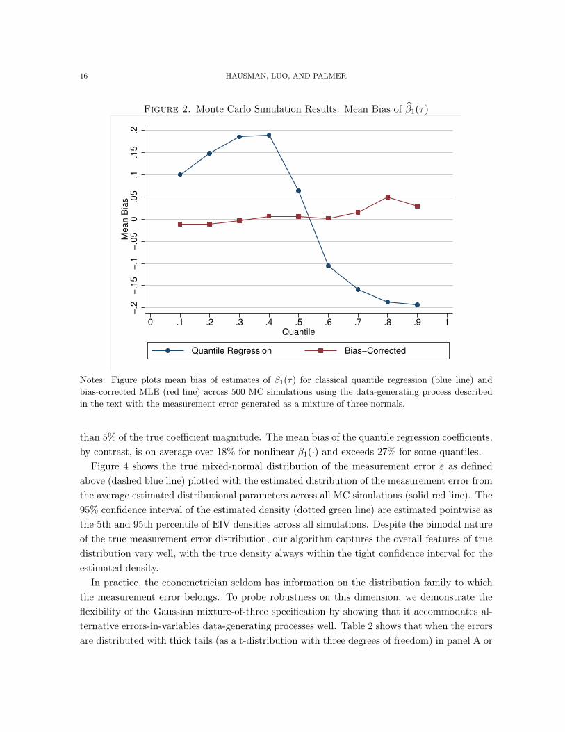
Figure 2. Monte Carlo Simulation Results: Mean Bias of b�1
(⌧)
−.2
−.1
5−
.1−
.05
0.0
5.1
.15
.2
Me
an
Bia
s
0 .1 .2 .3 .4 .5 .6 .7 .8 .9 1
Quantile
Quantile Regression Bias−Corrected
Notes: Figure plots mean bias of estimates of �1(⌧) for classical quantile regression (blue line) andbias-corrected MLE (red line) across 500 MC simulations using the data-generating process describedin the text with the measurement error generated as a mixture of three normals.
than 5% of the true coefficient magnitude. The mean bias of the quantile regression coefficients,by contrast, is on average over 18% for nonlinear �
1
(·) and exceeds 27% for some quantiles.Figure 4 shows the true mixed-normal distribution of the measurement error " as defined
above (dashed blue line) plotted with the estimated distribution of the measurement error fromthe average estimated distributional parameters across all MC simulations (solid red line). The95% confidence interval of the estimated density (dotted green line) are estimated pointwise asthe 5th and 95th percentile of EIV densities across all simulations. Despite the bimodal natureof the true measurement error distribution, our algorithm captures the overall features of truedistribution very well, with the true density always within the tight confidence interval for theestimated density.
In practice, the econometrician seldom has information on the distribution family to whichthe measurement error belongs. To probe robustness on this dimension, we demonstrate theflexibility of the Gaussian mixture-of-three specification by showing that it accommodates al-ternative errors-in-variables data-generating processes well. Table 2 shows that when the errorsare distributed with thick tails (as a t-distribution with three degrees of freedom) in panel A or
ERRORS IN THE DEPENDENT VARIABLE OF QUANTILE REGRESSION MODELS 17
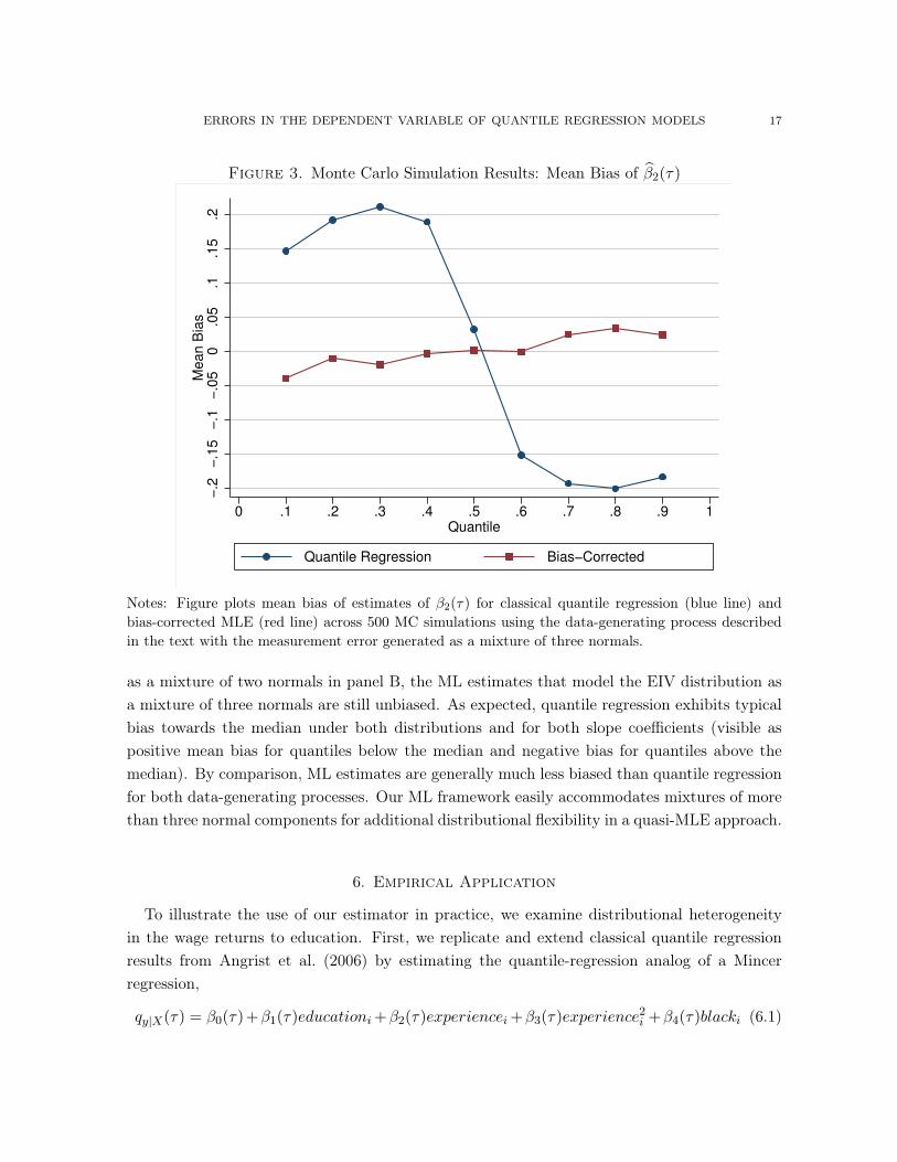
Figure 3. Monte Carlo Simulation Results: Mean Bias of b�2
(⌧)
−.2
−.1
5−
.1−
.05
0.0
5.1
.15
.2
Me
an
Bia
s
0 .1 .2 .3 .4 .5 .6 .7 .8 .9 1
Quantile
Quantile Regression Bias−Corrected
Notes: Figure plots mean bias of estimates of �2(⌧) for classical quantile regression (blue line) andbias-corrected MLE (red line) across 500 MC simulations using the data-generating process describedin the text with the measurement error generated as a mixture of three normals.
as a mixture of two normals in panel B, the ML estimates that model the EIV distribution asa mixture of three normals are still unbiased. As expected, quantile regression exhibits typicalbias towards the median under both distributions and for both slope coefficients (visible aspositive mean bias for quantiles below the median and negative bias for quantiles above themedian). By comparison, ML estimates are generally much less biased than quantile regressionfor both data-generating processes. Our ML framework easily accommodates mixtures of morethan three normal components for additional distributional flexibility in a quasi-MLE approach.
6. Empirical Application
To illustrate the use of our estimator in practice, we examine distributional heterogeneityin the wage returns to education. First, we replicate and extend classical quantile regressionresults from Angrist et al. (2006) by estimating the quantile-regression analog of a Mincerregression,
qy|X
(⌧) = �0
(⌧)+�1
(⌧)educationi
+�2
(⌧)experiencei
+�3
(⌧)experience2i
+�4
(⌧)blacki
(6.1)

18 HAUSMAN, LUO, AND PALMER
Figure 4. Monte Carlo Simulation Results: Distribution of Measurement Error
0.0
5.1
.15
.2.2
5
De
nsity
−8 −6 −4 −2 0 2 4 6 8
Measurement Error
True Density Estimated Density 95% CI
Notes: Figure reports the true measurement error (dashed blue line), a mean-zero mixture of threenormals (N (�3, 1), N (2, 1), and N (4, 1) with weights 0.5, 0.25, and 0.25, respectively) against theaverage density estimated from the 500 Monte Carlo simulations (solid red line). For each grid point,the dotted green line plots the 5th and 95th percentile of the EIV density function across all MCsimulations.
where qy|X
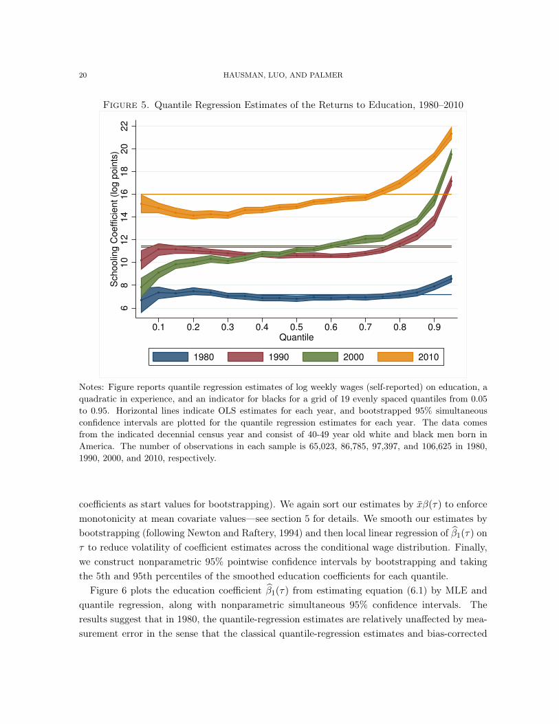
(⌧) is the ⌧ th quantile of the conditional (on the covariates X) log-wage distribu-tion, the education and experience variables are measured in years, and black is an indicatorvariable.7 Figure 5 plots results of estimating equation (6.1) by quantile regression on censusmicrodata samples from four decennial census years: 1980, 1990, 2000, and 2010, along withsimultaneous confidence intervals obtained from 200 bootstrap replications.8 Horizontal lines inFigure 5 represent OLS estimates of equation 5 for comparison. Consistent with the results inFigure 2 of Angrist et al., we find quantile-regression evidence that heterogeneity in the returnsto education across the conditional wage distribution has increased over time. In 1980, an addi-tional year of education was associated with a 7% increase in wages across all quantiles, nearly7Here we emphasize that, in contrast to the linear Mincer equation, quantile regression assumes that all unob-served heterogeneity enters through the unobserved rank of person i in the conditional wage distribution. Thepresence of an additive error term, which could include both measurement error and wage factors unobservedby the econometrician, would bias the estimation of the coefficient function �(·).8The 1980–2000 data come from Angrist et al.’s IPUMS query, and the 2010 follow their sample selection criteriaand again draw from IPUMS (Ruggles et al., 2015). For further details on the data including summary statistics,see Appendix B.
ERRORS IN THE DEPENDENT VARIABLE OF QUANTILE REGRESSION MODELS 19
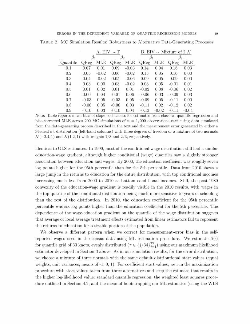
Table 2. MC Simulation Results: Robustness to Alternative Data-Generating Processes
A. EIV ⇠ T B. EIV ⇠ Mixture of 2 N�1
�2
�1
�2
Quantile QReg MLE QReg MLE QReg MLE QReg MLE0.1 0.07 0.01 0.09 -0.03 0.14 0.04 0.18 0.030.2 0.05 -0.02 0.06 -0.02 0.15 0.05 0.16 0.000.3 0.04 -0.02 0.05 -0.06 0.09 0.05 0.09 0.000.4 0.03 0.00 0.03 -0.02 0.03 0.05 -0.01 0.010.5 0.01 0.02 0.01 0.01 -0.02 0.08 -0.06 0.020.6 0.00 0.04 -0.01 0.06 -0.06 0.03 -0.09 0.030.7 -0.03 0.05 -0.03 0.05 -0.09 0.05 -0.11 0.000.8 -0.06 0.05 -0.06 0.03 -0.11 0.02 -0.12 0.020.9 -0.10 0.03 -0.10 0.04 -0.13 -0.02 -0.11 -0.04
Note: Table reports mean bias of slope coefficients for estimates from classical quantile regression andbias-corrected MLE across 200 MC simulations of n = 1, 000 observations each using data simulatedfrom the data-generating process described in the text and the measurement error generated by either aStudent’s t distribution (left-hand columns) with three degrees of freedom or a mixture of two normalsN (�2.4, 1) and N (1.2, 1) with weights 1/3 and 2/3, respectively.
identical to OLS estimates. In 1990, most of the conditional wage distribution still had a similareducation-wage gradient, although higher conditional (wage) quantiles saw a slightly strongerassociation between education and wages. By 2000, the education coefficient was roughly sevenlog points higher for the 95th percentile than for the 5th percentile. Data from 2010 shows alarge jump in the returns to education for the entire distribution, with top conditional incomesincreasing much less from 2000 to 2010 as bottom conditional incomes. Still, the post-1980convexity of the education-wage gradient is readily visible in the 2010 results, with wages inthe top quartile of the conditional distribution being much more sensitive to years of schoolingthan the rest of the distribution. In 2010, the education coefficient for the 95th percentilepercentile was six log points higher than the education coefficient for the 5th percentile. Thedependence of the wage-education gradient on the quantile of the wage distribution suggeststhat average or local average treatment effects estimated from linear estimators fail to representthe returns to education for a sizable portion of the population.
We observe a different pattern when we correct for measurement-error bias in the self-reported wages used in the census data using ML estimation procedure. We estimate �(·)for quantile grid of 33 knots, evenly distributed (⌧ 2 {j/34}33
j=1
) using our maximum likelihoodestimator developed in Section 3 above. As in our simulation results, for the error distribution,we choose a mixture of three normals with the same default distributional start values (equalweights, unit variances, means of -1, 0, 1). For coefficient start values, we run the maximizationprocedure with start values taken from three alternatives and keep the estimate that results inthe higher log-likelihood value: standard quantile regression, the weighted least squares proce-dure outlined in Section 4.2, and the mean of bootstrapping our ML estimates (using the WLS
20 HAUSMAN, LUO, AND PALMER
Figure 5. Quantile Regression Estimates of the Returns to Education, 1980–2010
68
10
12
14
16
18
20
22
Sch
oo
lin
g C
oe
ffic
ien
t (lo
g p
oin
ts)
0.1 0.2 0.3 0.4 0.5 0.6 0.7 0.8 0.9
Quantile
1980 1990 2000 2010
Notes: Figure reports quantile regression estimates of log weekly wages (self-reported) on education, aquadratic in experience, and an indicator for blacks for a grid of 19 evenly spaced quantiles from 0.05to 0.95. Horizontal lines indicate OLS estimates for each year, and bootstrapped 95% simultaneousconfidence intervals are plotted for the quantile regression estimates for each year. The data comesfrom the indicated decennial census year and consist of 40-49 year old white and black men born inAmerica. The number of observations in each sample is 65,023, 86,785, 97,397, and 106,625 in 1980,1990, 2000, and 2010, respectively.
coefficients as start values for bootstrapping). We again sort our estimates by x̄�(⌧) to enforcemonotonicity at mean covariate values—see section 5 for details. We smooth our estimates bybootstrapping (following Newton and Raftery, 1994) and then local linear regression of b�
1
(⌧) on⌧ to reduce volatility of coefficient estimates across the conditional wage distribution. Finally,we construct nonparametric 95% pointwise confidence intervals by bootstrapping and takingthe 5th and 95th percentiles of the smoothed education coefficients for each quantile.
Figure 6 plots the education coefficient b�1
(⌧) from estimating equation (6.1) by MLE andquantile regression, along with nonparametric simultaneous 95% confidence intervals. Theresults suggest that in 1980, the quantile-regression estimates are relatively unaffected by mea-surement error in the sense that the classical quantile-regression estimates and bias-corrected

ERRORS IN THE DEPENDENT VARIABLE OF QUANTILE REGRESSION MODELS 21
Figure 6. Returns to Education Correcting for LHS Measurement Error0
.05
.1.1
5.2
.25
.3.3
5.4
0 .2 .4 .6 .8 1
quantile
1980
0.0
5.1
.15
.2.2
5.3
.35
.4
0 .2 .4 .6 .8 1
quantile
1990
0.0
5.1
.15
.2.2
5.3
.35
.4
0 .2 .4 .6 .8 1
quantile
2000
0.0
5.1
.15
.2.2
5.3
.35
.4
0 .2 .4 .6 .8 1
quantile
2010
MLE Quantile Regression 95% CI
Notes: Graphs plot education coefficients estimated using quantile regression (red lines) and the MLestimator described in the text (blue line). Green dashed lines plot 95% Confidence Intervals using thebootstrap procedure described in the text. See notes to Figure (5).
ML estimates are nearly indistinguishable. For 1990, the pattern of increasing returns to edu-cation for higher quantiles is again visible in the ML estimates with the very highest quantilesseeing an approximately five log point larger increase in the education-wage gradient thansuggested by quantile regression, although this difference for top quantiles does not appearstatistically significant given typically wide confidence intervals for extremal quantiles. In the2000 decennial census, the quantile-regression and ML estimates of the returns to educationagain diverge for top incomes, with the point estimate suggesting that after correcting for mea-surement error in self-reported wages, the true returns to an additional year of education forthe top of the conditional wage distribution was a statistically significant 13 log points (17percentage points) higher than estimated by classical quantile regression. This bias correctionhas a substantial effect on the amount of inequality estimated in the education-wage gradient,with the ML estimates implying that top wage earners gained 23 log points (29 percentagepoints) more from a year of education than workers in the bottom three quartiles of wageearners. For 2010, both ML and classical quantile-regression estimates agree that the returnsto education increased across all quantiles, but again disagree about the marginal returns toschooling for top wage earners. Although the divergence between ML and quantile regressionestimates for the top quartile is not as stark as in 2000, the quantile regression estimates at the95th percentile of the conditional wage distribution are again outside the nonparametric 95%confidence intervals for the ML estimates.
22 HAUSMAN, LUO, AND PALMER
Figure 7. ML Estimated Returns to Education Across Years
0.0
5.1
.15
.2.2
5.3
.35
Education C
oeffic
ient
0 .1 .2 .3 .4 .5 .6 .7 .8 .9 1
Quantile
1980 1990 2000 2010
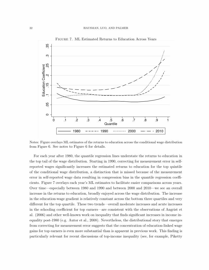
Notes: Figure overlays ML estimates of the returns to education across the conditional wage distributionfrom Figure 6. See notes to Figure 6 for details.
For each year after 1980, the quantile regression lines understate the returns to education inthe top tail of the wage distribution. Starting in 1990, correcting for measurement error in self-reported wages significantly increases the estimated returns to education for the top quintileof the conditional wage distribution, a distinction that is missed because of the measurementerror in self-reported wage data resulting in compression bias in the quantile regression coeffi-cients. Figure 7 overlays each year’s ML estimates to facilitate easier comparisons across years.Over time—especially between 1980 and 1990 and between 2000 and 2010—we see an overallincrease in the returns to education, broadly enjoyed across the wage distribution. The increasein the education-wage gradient is relatively constant across the bottom three quartiles and verydifferent for the top quartile. These two trends—overall moderate increases and acute increasesin the schooling coefficient for top earners—are consistent with the observations of Angrist etal. (2006) and other well-known work on inequality that finds significant increases in income in-equality post-1980 (e.g. Autor et al., 2008). Nevertheless, the distributional story that emergesfrom correcting for measurement error suggests that the concentration of education-linked wagegains for top earners is even more substantial than is apparent in previous work. This finding isparticularly relevant for recent discussions of top-income inequality (see, for example, Piketty

ERRORS IN THE DEPENDENT VARIABLE OF QUANTILE REGRESSION MODELS 23
Figure 8. Estimated Distribution of Wage Measurement Error
0.2
.4.6
.8
De
nsity
−2 −1.5 −1 −.5 0 .5 1 1.5 2
Measurement Error
Note: Graph plots the estimated probability density function of the measurement error in 1990 whenspecified as a mixture of three normal distributions.
and Saez, 2006). The time-varying nature of this relationship between the wage distributionand education is suggestive in the role of macroeconomic context in measuring the returns toeducation. If the wage earnings of highly educated workers at the top of the conditional wagedistribution is more volatile, then single-year snapshots of inequality may under or overstatethe relationship between wages and education. Judgment based solely on the 2000 pattern ofthe education gradient would find significantly more inequity in the returns to education thanestimates using 2010 data. By 2010, not only had the overall returns to education increasedacross nearly the entire wage distribution, but the particularly high education gradient enjoyedby the top quartile seems to have been smoothed out and shared by the top half of the wagedistribution. Whether the slight decrease in the schooling coefficient for top earners is simplya reflection of their higher exposure to the financial crisis (e.g. hedge-fund managers havinglarger declines in compensation than average workers) is a question to be asked of future data.
Our methodology also permits a characterization of the distribution of dependent-variablemeasurement error. Figure 8 plots the estimated distribution of the measurement error (solidblue line) in the 1990 data. Despite the flexibility afforded by the mixture specification, the

24 HAUSMAN, LUO, AND PALMER
Figure 9. 2000 Estimated Returns to Education: WLS vs. MLE0
.1.2
.3.4
0 .2 .4 .6 .8 1
quantile
WLS Quantile Regression MLE
estimated density is approximately normal—unimodal and symmetric but with higher kurtosis(fatter tails) than a single normal.
In light of the near-normality of the measurement error distribution estimated in the self-reported wage data, we report results for weighted-least squares estimates of the returns toeducation (see Section 4.2 for a discussion of the admissibility of the WLS estimator when theEIV distribution is normal). Figure 9 shows the estimated education-wage gradient across theconditional wage distribution for three estimators—quantile regression, weighted least squares,and MLE. Both the WLS and MLE estimates revise the right-tail estimates of the relationshipbetween education and wages significantly, suggesting that the quantile regression-based esti-mates for the top quintile of the wage distribution are severely biased from dependent-variableerrors in variables. The WLS estimates seem to be particularly affected by the extremal quan-tile problem (see, e.g. Chernozhukov, 2005), leading us to omit unstable estimates in the topand bottom deciles of the conditional wage distribution. While we prefer our MLE estimator,the convenience of the weighted least squares estimator lies in its ability to recover many of thequalitative facts obscured by LHS measurement error bias in quantile regression without theex-post smoothing (apart from dropping bottom- and top-decile extremal quantile estimates)required to interpret the ML estimates.

ERRORS IN THE DEPENDENT VARIABLE OF QUANTILE REGRESSION MODELS 25
7. Conclusion
In this paper, we develop a methodology for estimating the functional parameter �(·) inquantile regression models when there is measurement error in the dependent variable. Assum-ing that the measurement error follows a distribution that is known up to a finite-dimensionalparameter, we establish general convergence speed results for the MLE-based approach. Undera discontinuity assumption (C8), we establish the convergence speed of the sieve-ML estimator.When the distribution of the EIV is normal, optimization problem becomes an EM problemthat can be computed with iterative weighted least squares. We prove the validity of boot-strapping based on asymptotic normality of our estimator and suggest using a nonparametricbootstrap procedure for inference. Monte Carlo results demonstrate substantial improvementsin mean bias of our estimator relative to classical quantile regression when there are modesterrors in the dependent variable, highlighted by the ability of our estimator to estimate thesimulated underlying measurement error distribution (a bimodal mixture of three normals)with a high-degree of accuracy.
Finally, we revisited the Angrist et al. (2006) question of whether the returns to educa-tion across the wage distribution have been changing over time. We find a somewhat differentpattern than prior work, highlighting the importance of correcting for errors in the dependentvariable of conditional quantile models. When we correct for likely measurement error in theself-reported wage data, we find that top wages have grown much more sensitive to educa-tion than wage earners in the bottom three quartiles of the conditional wage distribution, animportant source of secular trends in income inequality.

26 HAUSMAN, LUO, AND PALMER
References
[1] Joshua Angrist, Victor Chernozhukov, and Iván Fernández-Val. Quantile regression under misspecification,with an application to the us wage structure. Econometrica, 74(2):539–563, 2006.
[2] David H Autor, Lawrence F Katz, and Melissa S Kearney. Trends in us wage inequality: Revising therevisionists. The Review of economics and statistics, 90(2):300–323, 2008.
[3] Songnian Chen. Rank estimation of transformation models. Econometrica, 70(4):1683–1697, 2002.[4] Xiaohong Chen. Large sample sieve estimation of semi-nonparametric models. Handbook of Econometrics,
6:5549–5632, 2007.[5] Xiaohong Chen and Demian Pouzo. Sieve quasi likelihood ratio inference on semi/nonparametric conditional
moment models1. 2013.[6] Victor Chernozhukov. Extremal quantile regression. Annals of Statistics, pages 806–839, 2005.[7] Victor Chernozhukov, Ivan Fernandez-Val, and Alfred Galichon. Improving point and interval estimators
of monotone functions by rearrangement. Biometrika, 96(3):559–575, 2009.[8] Stephen R Cosslett. Efficient semiparametric estimation of censored and truncated regressions via a
smoothed self-consistency equation. Econometrica, 72(4):1277–1293, 2004.[9] Stephen R Cosslett. Efficient estimation of semiparametric models by smoothed maximum likelihood*.
International Economic Review, 48(4):1245–1272, 2007.[10] Arthur P Dempster, Nan M Laird, Donald B Rubin, et al. Maximum likelihood from incomplete data via
the em algorithm. Journal of the Royal statistical Society, 39(1):1–38, 1977.[11] Jianqing Fan. On the optimal rates of convergence for nonparametric deconvolution problems. The Annals
of Statistics, pages 1257–1272, 1991.[12] Jerry Hausman. Mismeasured variables in econometric analysis: problems from the right and problems
from the left. Journal of Economic Perspectives, 15(4):57–68, 2001.[13] Jerry A Hausman, Jason Abrevaya, and Fiona M Scott-Morton. Misclassification of the dependent variable
in a discrete-response setting. Journal of Econometrics, 87(2):239–269, 1998.[14] Jerry A Hausman, Andrew W Lo, and A Craig MacKinlay. An ordered probit analysis of transaction stock
prices. Journal of financial economics, 31(3):319–379, 1992.[15] Joel L Horowitz. Applied nonparametric instrumental variables estimation. Econometrica, 79(2):347–394,
2011.[16] Thomas Kühn. Eigenvalues of integral operators with smooth positive definite kernels. Archiv der Mathe-
matik, 49(6):525–534, 1987.[17] Michael A Newton and Adrian E Raftery. Approximate bayesian inference with the weighted likelihood
bootstrap. Journal of the Royal Statistical Society. Series B (Methodological), pages 3–48, 1994.[18] Thomas Piketty and Emmanuel Saez. The evolution of top incomes: A historical and international per-
spective. The American Economic Review, pages 200–205, 2006.[19] Steven Ruggles, Katie Genadek, Ronald Goeken, Josiah Grover, and Matthew Sobek. Integrated public use
microdata series version 6.0 [machine-readable database], Minneapolis: University of Minnesota, 2015.[20] Susanne M Schennach. Quantile regression with mismeasured covariates. Econometric Theory, 24(04):1010–
1043, 2008.[21] Xiaotong Shen et al. On methods of sieves and penalization. The Annals of Statistics, 25(6):2555–2591,
1997.[22] Ying Wei and Raymond J Carroll. Quantile regression with measurement error. Journal of the American
Statistical Association, 104(487), 2009.

ERRORS IN THE DEPENDENT VARIABLE OF QUANTILE REGRESSION MODELS 27
Appendix A. Optimization Details
In this section, for practitioner convenience, we provide additional details on our optimizationroutine, including analytic characterizations of the gradient of the log-likelihood function. Forconvenience, we will refer to the log-likelihood l for observation i as
l = log
ˆ1
0
f"
(y � x�(⌧))d⌧
where " is distributed as a mixture of L normal distributions, with probability density function
f"
(u) =L
X
`=1
⇡`
�`
�
✓
u� µ`
�`
◆
.
For the mixture of normals, the probability weights ⇡`
on each component ` must sum to unity.Similarly, for the measurement error to be mean zero,
P
`
µ`
⇡`
= 0, where µ`
is the mean ofeach component. For a three-component mixture, this pins down
µ3
= �µ1
⇡1
+ µ2
⇡2
1� ⇡1
� ⇡2
(wherein we already used ⇡3
= 1�⇡1
�⇡2
). We also need to require that each weight be boundedby [0, 1]. To do this, we used a constrained optimizer and require that each of ⇡
1
,⇡2
, 1�⇡1
�⇡2
�0.01. The constraints on the variance of each component are that �2
`
� 0.01 for each `.Using the piecewise constant form of �(·), let �(⌧) be defined as
�(⌧) =
8
>
>
>
<
>
>
>
:
�1
when ⌧0
⌧ < ⌧1
�2
when ⌧1
⌧ < ⌧2
· · · · · ·�T
when ⌧T �1
⌧ < ⌧T
where ⌧0
= 0 and ⌧T
= 1. Ignoring the constraints on the weight and mean of the last mixturecomponent for the moment, the first derivatives of l with respect to each coefficient �
j
anddistributional parameter are
@l
@⇡`
=
1´1
0
f"
(y � x�(⌧))d⌧
ˆ1
0
1
�`
�
✓
y � x�(⌧)� µ`
�`
◆
d⌧
@l
@µ`
=
1´1
0
f"
(y � x�(⌧))d⌧
ˆ1
0
⇡`
�`
✓
y � x�(⌧)� µ`
�2`
◆
�
✓
y � x�(⌧)� µ`
�`
◆
d⌧
@l
@�`
=
1´1
0
f"
(y � x�(⌧))d⌧
ˆ1
0
�⇡`
�2`
�
✓
y � x�(⌧)� µ`
�`
◆
d⌧
+
1´1
0
f"
(y � x�(⌧))d⌧
ˆ1
0
1
�`
✓
(y � x�(⌧)� µ`
)
2
�3`
◆
�
✓
y � x�(⌧)� µ`
�`
◆
d⌧
28 HAUSMAN, LUO, AND PALMER
@l
@�j
=
1´1
0
f"
(y � x�(⌧))d⌧
ˆ⌧
j
⌧
j�1
@f"
(y � x�j
)
@�j
d⌧
=
1´1
0
f"
(y � x�(⌧))d⌧(⌧
j
� ⌧j�1
)
@f"
(y � x�j
)
@�j
=
(⌧j
� ⌧j�1
)´1
0
f"
(y � x�(⌧))d⌧f 0
"
(y � x�j
) (�x)
=
� (⌧j
� ⌧j�1
)x´1
0
f"
(y � x�(⌧))d⌧
3
X
`=1
⇡`
�2`
�
✓
y � x�j
� µ`
�`
◆✓
�y � x�j
� µ`
�`
◆
.
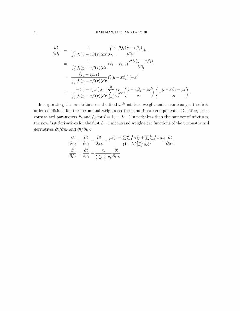
Incorporating the constraints on the final Lth mixture weight and mean changes the first-order conditions for the means and weights on the penultimate components. Denoting theseconstrained parameters ⇡̃
`
and µ̃`
for ` = 1, . . . L� 1 strictly less than the number of mixtures,the new first derivatives for the first L�1 means and weights are functions of the unconstrainedderivatives @l/@⇡
`
and @l/@µ`
:
@l
@⇡̃`
=
@l
@⇡`
� @l
@⇡L
� µ`
(1�P
L�1
`=1
⇡`
) +
P
L�1
`=1
⇡`
µ`
(1�P
L�1
`=1
⇡`
)
2
@l
@µL
@l
@µ̃`
=
@l
@µ`
� ⇡`
P
L�1
`=1
⇡`
@l
@µL

ERRORS IN THE DEPENDENT VARIABLE OF QUANTILE REGRESSION MODELS 29
Appendix B. Data Appendix
Following the sample selection criteria of Angrist et al. (2006), our data comes from 1%samples of decennial census data available via IPUMS.org (Ruggles et al., 2015) from 1980–2010. From each database, we select annual wage income, education, age, and race data forprime-age (age 40-49) black and white males who have at least five years of education, wereborn in the United States, had positive earnings and hours worked in the reference year, andwhose responses for age, education, and earnings were not imputed. Our dependent variable islog weekly wage, obtained as annual wage income divided by weeks worked. For 1980, we takethe number of years of education to be the highest grade completed and follow the methodologyof Angrist et al. (2006) to convert the categorical education variable in 1990, 2000, and 2010into a measure of the number of years of schooling. Experience is defined as age minus yearsof education minus five. For 1980, 1990, and 2000, we use the exact extract of Angrist etal., and draw our own data to extend the data to include the 2010 census. Table 3 reportssummary statistics for the variables used in the regressions in the text. Wages for 1980–2000were expressed in 1989 dollars after deflating using the Personal Consumption ExpendituresIndex. As slope coefficients in a log-linear quantile regression specification are unaffected byscaling the dependent variable, we do not deflate our 2010 data.
Table 3. Education and Wages Summary StatisticsYear 1980 1990 2000 2010Log weekly wage 6.40 6.46 6.47 8.34
(0.67) (0.69) (0.75) (0.78)Education 12.89 13.88 13.84 14.06
(3.10) (2.65) (2.40) (2.37)Experience 25.46 24.19 24.50 24.60
(4.33) (4.02) (3.59) (3.82)Black 0.076 0.077 0.074 0.078
(0.27) (0.27) (0.26) (0.27)Number of Observations 65,023 86,785 97,397 106,625
Notes: Table reports summary statistics for the Census data used in the quantile wage regressions inthe text. The 1980, 1990, and 2000 datasets come from Angrist et al. (2006). Following their sampleselection, we extended the sample to include 2010 Census microdata from IPUMS.org (Ruggles et al.,2015).

30 HAUSMAN, LUO, AND PALMER
Appendix C. Deconvolution Method
Although the direct MLE method is used to obtain identification and some asymptoticproperties of the estimator, the main asymptotic property of the maximum likelihood estimatordepends on discontinuity assumption C.9. Evodokimov (2011) establishes a method usingdeconvolution to solve a similar problem under panel data condition. He adopts a nonparametricsetting and therefore needs kernel estimation method.
Instead, in the special case of quantile regression setting, we can further explore the linearstructure without using the nonparametric method. Deconvolution offers a straight forwardview of the estimation procedure.
The CDF function of a random variable w can be computed from the characteristic function�w
(s).
F (w) =1
2
� lim
q!1
ˆq
�q
e�iws
2⇡is�w
(s)ds. (C.1)
�0
(⌧) satisfying the following conditional moment condition:
E[F (x�0
(⌧)|x)] = ⌧. (C.2)
Since we only observe y = x�(⌧) + ", the �x�
(s) = E[exp(isy)]
�
"
(s)
. Therefore �0
(⌧) satisfies:
E[
1
2
� ⌧ � lim
q!1
ˆq
�q
E[e�i(y�x�0(⌧))s|x]2⇡is�
"
(s)ds|x] = 0 (C.3)
In the above expression, the limit symbol before the integral can not be exchanged with thefollowed conditional expectation symbol. But in practice, they can be exchanged if the integralis truncated.
A simple way to explore information in the above conditional moment equation is to considerthe following moment conditions:
E
"
x
1
2
� ⌧ + Im( lim
q!1
ˆq
�q
E[e�i(y�x�0(⌧))s|x]2⇡s�
"
(s)ds)
!#
= 0 (C.4)
Let F (x�, y, ⌧, q) = 1
2
� ⌧ � Imn´
q
�q
e
�i(y�x�)s|x
2⇡s�
"
(s)
dso
.Given fixed truncation threshold q, the optimal estimator of the kind E
n
[f(x)F (x�, y, ⌧, q)]
is:
En
[E[
@F
@�|x]/�(x)2F (x�, y, ⌧, q)] = 0, (C.5)
where �(x)2 := E[F (x�, y, ⌧)2|x].Another convenient estimator is:

ERRORS IN THE DEPENDENT VARIABLE OF QUANTILE REGRESSION MODELS 31
argmin
�
En
[F (x�, y, ⌧, q)2]. (C.6)
These estimators have similar behaviors in term of convergence speed, so we will only discussthe optimal estimator. Although it can not be computed directly because the weight @F
@�
/�(x)2
depends on �, it can be achieved by an iterative method.
Theorem 3. (a) Under condition OS with � � 1, the estimator � satisfying equation (3.15)with truncation threshold q
n
= CN12� satisfies:
� � �0
= O(N�1N
2�), (C.7)
(b) Under condition SS with, the estimator b� satisfies equation (3.15) with truncation thresh-old q
n
= C log(n)1� satisfies:
� � �0
= O(log(n)�1�
). (C.8)

32 HAUSMAN, LUO, AND PALMER
Appendix D. Proofs of Lemmas and Theorems
D.1. Lemmas and Theorems in Section 2. In this section we prove the Lemmas andTheorems in section 2.
Proof of Lemma 1.
Proof. For any sequence of monotone functions f1
, f2
, ..., fn
, ... with each one mapping [a, b] intosome closed interval [c, d]. For bounded monotonic functions, point convergence means uniformconvergence, therefore this space is compact. Hence the product space B
1
⇥ B2
⇥ ... ⇥ Bk
iscompact. It is complete since L2 functional space is complete and limit of monotone functionsis still monotone. ⇤
Proof of Lemma 2.
Proof. WLOG, under condition C.1-C.3, we can assume the variable x1
is continuous. If thereexists �(·) and f(·) which generates the same density g(y|x,�(·), f) as the true paramter �
0
(·)and f
0
(·), then by applying Fourier transformation,
�(s)
ˆ1
0
exp(is�(⌧))d⌧ = �0
(s)
ˆ1
0
exp(is�0
(⌧))d⌧.
Denote m(s) = �(s)
�0(s)= 1 +
P
1
k=2
ak
(is)k around a neighborhood of 0. Therefore,
m(s)
ˆ1
0
exp(isx�1
��1
(⌧))1
X
i=0
(is)kxk1
�1
(⌧)k
k!d⌧ =
ˆ1
0
exp(isx�1
�0,�1
(⌧))1
X
i=0
(is)kxk1
�0,1
(⌧)k
k!d⌧.
Since x1
is continuous, then it must be that the corresponding polynomials of x1
are the samefor both sides. Namely,
m(s)(is)k
k!
ˆ1
0
exp(isx�1
��1
(⌧))�1
(⌧)kd⌧ =
(is)k
k!
ˆ1
0
exp(isx�1
�0.�1
(⌧))�0,1
(⌧)kd⌧.
Divide both sides of the above equation by (is)k/k!, as let s approaching 0, we get:
ˆ1
0
�1
(⌧)kd⌧ =
ˆ1
0
�0,1
(⌧)kd⌧.
By assumption C.2, �1
(·) and �0,1
(·) are both strictly monotone, differentiable and greaterthan or equal to 0. So �
1
(⌧) = �0,1
(⌧) for all ⌧ 2 [0, 1].Now consider the same equation considered above. divide both sides by (is)k/k!, we get
m(s)´1
0
exp(isx�1
��1
(⌧))�0,1
(⌧)kd⌧ =
´1
0
exp(isx�1
�0.�1
(⌧))�0,1
(⌧)kd⌧,for all k � 0.Since �
0,1
(⌧)k, k � 1 is a functional basis of L2
[0, 1], therefore m(s) exp(isx�1
��1
(⌧)) =
exp(isx�1
�0,�1
(⌧)) for all s in a neighborhood of 0 and all ⌧ 2 [0, 1]. If we differentiate bothsides with respect to s and evaluate at 0 (notice that m0
(0) = 0), we get:

ERRORS IN THE DEPENDENT VARIABLE OF QUANTILE REGRESSION MODELS 33
x�1
��1
(⌧) = x�1
�0,�1
(⌧),
for all ⌧ 2 [0, 1].
By assumption C.2, E[x0x] is non-singular. Therefore E[x0�1
x�1
] is also non-singular. Hence,the above equation suggests �
�1
(⌧) = �0,�1
(⌧), for all ⌧ 2 [0, 1]. Therefore, �(⌧) = �0
(⌧).Thisimplies that �(s) = �
0
(s). Hence f(") = f0
(").⇤
Proof of Lemma 3.
Proof. Proof: (a) If the equation stated in (a) holds a.e., then we can apply Fourier transfor-mation on both sides, i.e., conditional on x,
ˆeisyˆ
1
0
fy
(y � x�(⌧))xt(⌧)d⌧dy =
ˆeisyˆ
1
0
ˆ1
0
f�
(y � x�(⌧))d⌧dy. (D.1)
Let q(⌧) = x�(⌧), which is a strictly increasing function. We can use change of variables tochange ⌧ to q.
We get:ˆ1
0
eisx�(⌧)xt(⌧)
ˆeis(y�x�(⌧))f 0
(y�x�(⌧))dyd⌧ =
ˆ1
0
eisx�(⌧)ˆ
eis(y�x�(⌧))f�
(y�x�(⌧))dyd⌧.
(D.2)or, equivalently,
ˆ1
0
eisx�(⌧)xt(⌧)d⌧(�is)�"
(s) =
ˆ1
0
eisx�(⌧)d⌧@�
"
(s)
@�, (D.3)
given that´f 0
(y)eisydy = �is´f(y)eisydy.
Denote´1
0
eisx�(⌧)xt(⌧)d⌧ = q(x, s), and´1
0
eisx�(⌧)d⌧ = r(x, s). Therefore,
�isq(s, x)�(s) = r(s, x)@�
"
(s)
@�.
First we consider normal distribution. �"
(s) = exp(��2s2/2). So @�
"
(s)
@�
= ��s2�"
(s).Therefore, q(s, x) = is�r(s, x), for all s and x with positive probability. Since x�(⌧) is
strictly increasing, let z = x�(⌧), and I(y) = 1(x�(0) y x�(1)).So q(s, x) =
´1
�1
eisw{ xt(z
�1(w))
xz
0(z
�1(w))
I(w)}dw, and r(s, x) =´1
�1
eisw{ 1
xz
0(z
�1(w))
I(w)}dw.q(s, x) = is�r(s, x) means that there is a relationship between the integrands. More specifi-
cally, it must be that
xt(z�1
(w))
xz0(z�1
(w))I(w) = d
1
xz0(z�1
(w))I(w)/dw. (D.4)
Obviously they don’t equal to each other for a continuous interval of xi
, because the latterfunction has a � function component.

34 HAUSMAN, LUO, AND PALMER
For more general distribution function f , �isq(s, x)�"
(s) = r(s, x)@�"
(s)
@�
, with @�
"
(s)
@�
=
�"
(s)s2m(s), for some m(s) :=P
1
j=0
aj
(is)j .Therefore,
�ism(s)r(s, x) = q(s, x).
Consider local expansion of s in both sides, we get:
�is(1
X
j=0
aj
(is)j)(1
X
k=0
ˆ1
0
(x�(⌧))kd⌧(is)k
k!) =
1
X
j=0
ˆ1
0
(x�(⌧))kxt(⌧)d⌧(is)k
k!.
Compare the kth polynomial of s, we get:´1
0
(x�(⌧))kxt(⌧)d⌧ = 0, if k = 0.´1
0
(x�(⌧))kxt(⌧)d⌧ = �P
1j<k
aj
(is)j(´1
0
x�(⌧))j�1d⌧ (is)
j�1
(j�1)!
.Let x
1
be the continuous variable, and x�1
be the variables left. Let �1
be the coefficientcorresponds to x
1
and let ��1
be the coefficient corresponds to x�1
. Let t1
be the componentin t that corresponds to x
1
, and let t�1
be the component in t that corresponds to x�1
.Then, consider the (k + 1)
th order polynomial of x1
, we get:
ˆ1
0
�1
(⌧)kt1
(⌧)d⌧ = 0.
since �1
(⌧)k, k � 0 form a functional basis in L2
[0, 1], t1
(⌧) must equal to 0.Consider the kth order polynomial of x
1
, we get:
ˆ1
0
�1
(⌧)k(x�1
t�1
(⌧))d⌧ = 0.
So x�1
t�1
(⌧) = 0 for all ⌧ 2 [0, 1]. Since E[x�1
x0�1
] has full rank, it must be that t�1
(⌧) = 0.Hence local identification condition holds. ⇤
D.2. Lemmas and Theorems in Section 3. In this subsection, we prove the Lemmas andTheorems in section 3.
Lemma 9 (Donskerness of ⇥). The parameter space ⇥ is Donsker.
Proof. By theorem 2.7.5 of Van der Vaart and Wellner (2000), the space of bounded monotonefunction, denoted as F , satisfies:
logN[]
(",F , Lr
(Q)) K1
",
for every probability measure Q and every r � 1, and a constant K which depends only onr.

ERRORS IN THE DEPENDENT VARIABLE OF QUANTILE REGRESSION MODELS 35
Since ⇥ is a product space of bounded monotone functions M and a finite dimensionalbounded compact set ⌃, therefore the bracketing number of ⇥ given any measure Q is alsobounded by:
logN[]
(",⇥, Lr
(Q)) Kdx
1
",
Therefore,´�
0
q
logN[]
(",⇥, Q) < 1, i.e., ⇥ is Donsker. ⇤
Proof of Lemma 4.
Proof. Ln
(✓) � Ln
(✓0
) by definition, and we know that L(✓0
) � L(✓) by information inequality.By Lemma 10, since ⇥ is Donsker, then the following stochastic equicontinuity condition
holds:
pn(L
n
(✓)� Ln
(✓1
)� (L(✓)� L(✓1
))) !p
rn
,
for some generic term rn
= op
(1), if |✓ � ✓1
| ⌘n
for small enough ⌘n
. Therefore uniformconvergence of L
n
(✓)� L(✓) holds in ⇥. In addition, by Lemma 2, the parameter ✓ is globallyidentified. Also, it is obvious that L is continuous in ✓.
Therefore, the usual consistency result of MLE estimator applies here. ⇤
Proof of Lemma 5.Proof of Lemma 6.
Proof. By definition,
En
[log(g(y|x,�,�))] � En
[log(g(y|x,�0
,�0
))]. (D.5)
And we know that by information inequality, E[log(g(y|x,�,�))] E[log(g(y|x,�0
,�0
))].
Therefore, E[log(g(y|x,�,�))]�E[log(g(y|x,�0
,�0
))] � 1
p
n
Gn
[log(g(y|x,�,�))�g(y|x,�0
,�0
))].By Donskerness of parameter space ⇥, the following equicontinuity condition holds:Hence,
0 E[log(g(y|x,�0
,�0
))]� E[log(g(y|x,�,�))] -p
1pn. (D.6)
Because � is converging to the true parameter inpn speed, we will simply use �
0
here inthe argument because it won’t affect our analysis later. In the notation, I will abbreviate �
0
.Let z(y, x) = g(y|�, x) � g(y|�
0
, x). In equation 3.19, we know that the KL-discrepancy ofg(y|x,�
0
) and g(y|x,�), noted as D(g(·|�0
)||g(·|�)), is bounded by C 1
p
n
with p ! 1.So E
x
[||z(y|x)||1
]
2 D(g(·|�0
)||g(·|�)) 2(E[log(g(y|x,�0
,�0
))] � E[log(g(y|x,�,�))]) -p
1
p
n
, where |z(y|x)|1
=
´1
�1
|z(y|x)|dy.Now consider the characteristic function of y conditional on x:

36 HAUSMAN, LUO, AND PALMER
�x�
(s) =
´1
�1
g(y|�, x)eisydy�"
(s),
and
�x�0(s) =
´1
�1
g(y|�0
, x)eisydy
�"
(s).
Therefore
�x�
(s)� �x�0(s) =
´1
�1
z(y|x)eisydy�"
(s), (D.7)
and |�x�
(s)� �x�0(s)|
||z(y|x)||1
|�
"
(s)|
.Let F
⌘
(w) = 1
2
� lim
q!1
´q
�q
e
�iws
2⇡s
�⌘
(s)ds. Then F (w) is the CDF of the random variable⌘.
Let F⌘
(w, q) = 1
2
�´q
�q
e
�iws
2⇡s
�⌘
(s)ds. If the p.d.f of ⌘ is a C1 function and ⌘ has finite secondorder moment, then F
⌘
(w, q) = F⌘
(w) + O(
1
q
2 ). Since x and � are bounded, let ⌘ = x�(⌧),then there exists a common C such that |F
x�
(w, q) � Fx�
(w)| C
q
2 for all x 2 X and w 2 Rfor q being large enough.
Therefore |Fx�
(w, q) � Fx�0(w, q)| = |
´q
�q
e
isw
2⇡s
(�x�
(s) � �x�0(s))ds| |
´q
�q
||z(y|x)||12⇡s
|�
"
(s)|
ds| -||z(y|x)||
1
�(q).Consider the follow moment condition:
E[x(Fx�0(x�0)� ⌧)] = 0 (D.8)
Let F0
denote Fx�0 and F denote F
x�
.We will replace the moment condition stated in (J.8) by the truncated function F (w, q). So
by the truncation property, for any fixed � 2 Rd
x :
�E[x(F0
(x�)� F0
(x�0
))] = �E[x(F0
(x�)� F (x�))] = �E[x(F0
(x�, q)� F (x�, q))] +O(
1
q2).
(D.9)The first term of the right hand side is bounded by:
E[|�x|�(q)||z(y|x)||1
] - E[||z(y|x)||1
]�(q).
And �E[x(F0
(x�)�F0
(x�0
))] = �E[x0xf(x�0
(⌧))](�(⌧)� �0
(⌧))(1+ o(1)), where f(x�0
(⌧))
is the p.d.f of the random variablex�0
(·) evaluated at ⌧ .Hence, �(⌧)� �
0
(⌧) = Op
(
�(q)
n
14) +O(
1
q
2 ).
Under OS condition, �(q) - q�, so by choosing q = Cn1
4(�+2) , ||�(⌧)� �0
(⌧)||2
-p
n�
12(�+2) .
Under SS condition, �(q) - C1
(1+ |q|C2) exp(|q|�/C
3
). By choosing q = C log(n)14� , ||�(⌧)�
�0
(⌧)||2
-p
log(n)�12� . ⇤

ERRORS IN THE DEPENDENT VARIABLE OF QUANTILE REGRESSION MODELS 37
D.3. Lemmas and Theorems in Sections 4 and 5. In this subsection we prove the Lemmasand Theorems in section 4.
Proof of Lemma 8.
Proof. Suppose f satisfies discontinuity condition C8 with degree � > 0.Denote l
k
= (f⌧1 , f⌧2 , ..., f⌧
k
, g�
).
For any (pk
, �) 2 Pk
, pk
Ik
p0k
= E[
´R
(l
k
p
0k
)
2
g
dy] � E[(lk
p0k
)
2
], since g is bounded from above.Assume c := inf
x2§,⌧2[0,1]
(x�0(⌧)) > 0. Now consider an interval [y, y + 1
2�kc
].Let S(�) :=
P
�
i=0
(�Ci
�
)
2, where Cb
a
stands for the combinatorial number choosing b elementsfrom a set with size a.
So,
S(�)E[
ˆR
(lk
p0k
)
2
dy] = E[
�
X
j=0
(Cj
�
)
2
ˆR(lk
(y + j/(2�ukc))p0k
(y + j/(2�kc)))2dy].
And by Cauchy-Schwarz inequality,
E[
�
X
j=0
(Cj
�
)
2
ˆR(lk
(y + j/(2�ukc))p0k
(y + j/(2�ukc)))2dy]
� E[
ˆR(
�
X
j=0
(�1)
jCj
�
lk
(y + j/(2�ukc))p0k
(y + j/(2�ukc)))2dy].
let J i
k
:= [a+ x�( i+1/2
k
)� 1
2�uk
, a+ x�( i+1/2
k
) +
1
2�uk
], so
E[
�
X
j=0
(Cj
�
)
2
ˆR(lk
(y + j/(2�ukc))p0k
(y + j/(2�ukc)))2dy]
� E[
ˆJ
i
k
(
�
X
j=0
(�1)
jCj
�
lk
(y + j/(2�ukc))p0k
(y + j/(2�ukc)))2dy].
By discontinuity assumption, ,�
X
j=0
(�1)
jCj
�
lk
(y + j/(2�ukc))p0k
(y + j/(2�ukc))
=
1
(uk)��1
(
c
(�� 1)!
xi
p0i
+
cj
uk
k
X
j=1,j 6=i
xj
pj
),
with cj
uniformly bounded from above, since f (�) is L1 Lipschitz except at a.Notice that J i
k
does not intersect each other, so S(�)E[
´R(lkp
0
k
)
2dy] � S(�)P
k
i=1
E[
´J
i
k
(lk
p0k
)
2dy]
� E[
c
0
2uk
P
k
i=1
{ 1
(uk)
��1 (c
(��1)!
xi
p0i
+
c
jk
uk
P
k
j=1,j 6=i
xj
pj
)}2]For constant u being large enough (only depend on �, sup c
jk
and c),

38 HAUSMAN, LUO, AND PALMER
E[
P
k
i=1
{ 1
(uk)
��1 (c
(��1)!
xi
p0i
+
c
jk
uk
P
k
j=1,j 6=i
xj
pj
)}2] � c(�) 1
k
2��1
P
k
j=1
E[x2j
p2j
] ⇣ 1
k
2� ||p||22
,with some constant c(�) only depends on � and u.In addition, from condition C5, we know that ✓I
k
✓ % ||�||22
.Therefore ✓I
k
✓ % ||�||22
+
1
k
2� ||p||22
% 1
k
2� ||✓||22
. Hence, the smallest eigenvalue r(Ik
) of Ik
isbounded by c
k
�
, with some generic constant c depending on �, x, the the L1 Lipshitz coefficientof f (k) at set R� [a� ⌘, a+ ⌘]. ⇤
Proof of Lemma 9.
Proof. The proof of this Lemma is based on Chen (2008) results of sieve extremum estimatorconsistency. Below I recall the five Conditions listed in Theorem 3.1 of Chen (2008). Theo-rem 3.1 in Chen (2008) shows that as long as the following conditions are satisfied, the sieveestimator is consistent.
Condition C11. [Identification] (1) L(✓0
) < 1, and if L(✓0
) = �1 then L(✓) > �1 for all✓ 2 ⇥
k
\ {✓0
} for all k � 1.(2)there are a nonincreasing positive function �(·) and a positive function m(·) such that for
all " > 0 and k � 1,
L(✓0
)� sup
✓2⇥
k
:d(✓,✓0)L(✓k
)�"
� �(k)m(") > 0.
Condition C12. [Sieve Space] ⇥
k
⇢ ⇥
k+1
⇢ ⇥ for all k � 1; and there exists a sequence⇡k
✓0
2 ⇥
k
such that d(✓0
,⇡k
✓0
) ! 0 as k ! 0.
Condition C13. [Continuity] (1)L(✓) is upper semicontinuous on ⇥
k
under metric d(·, ·).(2) |L(✓
0
)� L(⇡k(n)
✓0
)| = o(�(k(n))).
Condition C14. [compact Sieve space] ⇥k
is compact under d(·, ·).
Condition C15. [uniform convergence] 1) For all k � 1, plim sup
✓2⇥
k
|Ln
(✓) � L(✓)| = 0. 2)bc(k(n)) = o
p
(�(k(n))) where bc(k(n)) := sup
✓2⇥
k
|Ln
(✓)� L(✓)|. 3) ⌘k(n)
= o(�(k(n))).
These assumptions are verified below:For Identification: Let d be the metric induced by theL2 norm || · ||
2
defined on ⇥. Byassumption C4 and compactness of ⇥, L(✓
0
) � sup
✓2⇥:d(✓,✓0)L(✓
k
) > 0 for any " > 0. So let�(k) = 1, Identification condition holds.
For condition Sieve Space: Our Sieve space satisfies ⇥k
⇢ ⇥
2k
⇢ ⇥. In general we can considethe sequence ⇥
2
k(1) ,⇥2
k(2) , ...,⇥2
k(n) ... instead of ⇥
1
,⇥2
,⇥3
... with k(n) being an increasingfunction and lim
n!1
k(n) = 1.For condition Continuity: Since we assume f is continuous and L1 Lipshitz, (1) is satisfied.
(2) is statisfied under the construction of our Sieve space.Condition Compact Sieve Space is trivial.

ERRORS IN THE DEPENDENT VARIABLE OF QUANTILE REGRESSION MODELS 39
The condition Uniform Convergence is also easy to verify since the entropy metric of space⇥
k
is finite and uniformly bounded by the entropy metric of ⇥. Therefore we have stochasticequi-continuity, i.e., sup
✓2⇥
k
|Ln
(✓)� L(✓)| = Op
(
1
p
n
).
In (3), ⌘k
is defined as the error in the maximization procedure. Since � is constant, as soonas our maximizer b✓
k
satisfies Ln
(
b✓k
)� sup
✓2⇥
k
Ln
(✓k
) ! 0, (3) is verified.Hence, the Sieve MLE estimator is consistent.
⇤
Proof of Lemma 10.
Proof. This theorem follows directly from Lemma 8. If the neighborhood ·j
of ✓0
is chosen as�
j
:= {✓ 2 ⇥
k
: |✓ � ✓0
|2
µ
k
k
�
},with µ
k
being a sequence converging to 0, then the non-linear term in Ex
[
´Y
(g(y|x,✓0)�g(y|x,✓))
2
g(y|x,✓0)dy]
is dominated by the first order term ✓Ik✓0.⇤
Proof of Theorem 1.
Proof. Suppose ✓ = (�(·),�) 2 ⇥
k
is the Sieve estimator. By Lemma 8, the consistency ofSieve estimator shows that ||✓ � ✓
0
||2
!p
0.Denote ⌧
i
=
i�1
k
, i = 1, 2, ..., k
First order condition gives:
En
[�xf 0
(y � x�(⌧i
)|�)] = 0. (D.10)
andE
n
[g�
(y|x,�,�)] = 0. (D.11)
Assume that we choose k = k(n) such that:(1)k�+1||✓ � ✓
0
||2
!p
0.(2)kr||✓ � ✓
0
||2
! 1 with p ! 1.And assume that r > � + 1. Such sequence k(n) exists because Lemma 7 shows an upper
bound for ||✓ � ✓0
||, i.e., ||✓0
� ✓||2
-p
n�
12(2+�) .
From the first order condition, we know that:
En
[(
f⌧1(y|x, ✓), f⌧2(y|x, ✓), ..., f⌧
k
(y|x, ✓)g(y|x, ✓) ,
g�
(y|x, ✓)g(y|x, ✓) )] = 0.
Denote f✓
k
= (f⌧1(y|x, ✓), f⌧2(y|x, ✓), ..., f⌧
k
(y|x, ✓)).Therefore,
0 = En
[(
f✓
k
g,g�
g)] = (E
n
[(
f✓
k
g,g�
g)]� E
n
[(
f✓
k
,0
g0
,g�,0
g0
)]) + En
[(
f✓
k
,0
g0
,g�,0
g0
)].
The first term can be decomposed as:
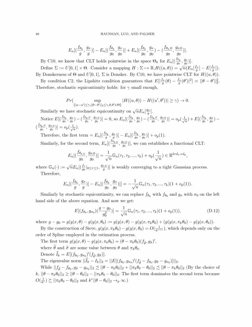
40 HAUSMAN, LUO, AND PALMER
En
[(
f✓
k
g,g�
g)]� E
n
[(
f✓
k
g0
,g�
g0
)] + En
[(
f✓
k
g0
,g�
g0
)� (
f✓
k
,0
g0
,g�,0
g0
)].
By C10, we know that CLT holds pointwise in the space ⇥
k
for En
[(
f
✓
k
g0, g�g0)].
Define ⌃ := U [0, 1] ⇥ ⇥. Consider a mapping H : ⌃ 7! R,H((u, ✓)) =pn(E
n
[
f
u
g
] � E[
f
u
g
]).By Donskerness of ⇥ and U [0, 1], ⌃ is Donsker. By C10, we have pointwise CLT for H((u, ✓)).
By condition C2, the Lipshitz condition guarantees that E[|fug
(✓) � f
u
g
(✓0)|2] ⇣ ||✓ � ✓0||22
.Therefore, stochastic equicontinuity holds: for � small enough,
Pr( sup
{|u�u
0|�,||✓�✓
0||2�,✓,✓
02⇥}
|H((u, ✓))�H((u0, ✓0))| � �) ! 0.
Similarly we have stochastic equicontinuity onpnE
n
[
g
�
g
].
Notice E[(
f
✓
k
g0, g�g0)� (
f
✓
k
,0
g0, g�,0
g0)] = 0, so E
n
[(
f
✓
k
g0, g�g0)� (
f
✓
k
,0
g0, g�,0
g0)] = o
p
(
1
p
n
)+E[(
f
✓
k
g0, g�g0)�
(
f
✓
k
,0
g0, g�,0
g0)] = o
p
(
1
p
n
).
Therefore, the first term = En
[(
f
✓
k
g
, g�g
)]� En
[(
f
✓
k
g0, g�g0)] + o
p
(1).
Similarly, for the second term, En
[(
f
✓
k,0
g0, g�,0
g0)], we can establishes a functional CLT:
En
[(
f✓
k,0
g0
,g�,0
g0
)] =
1pnG
n
(⌧1
, ⌧2
, ..., ⌧k
) + op
(
1pn) 2 Rkrd
x
+d
p ,
where Gn
(·) :=pnE
n
[(
f
⌧
g0|0⌧1
, g�,0g
)] is weakly converging to a tight Gaussian process.Therefore,
En
[(
f✓
k
g,g�
g)]� E
n
[(
f✓
k
g0
,g�
g0
)]] = � 1pnG
n
(⌧1
, ⌧2
, ..., ⌧k
)(1 + op
(1)).
Similarly by stochastic equicontinuity, we can replace f✓
k
with f✓0 and g
�
with �0
on the lefthand side of the above equation. And now we get:
E[(f✓0 , g�0)(
g � g0
g20
)] =
1pnG
n
(⌧1
, ⌧2
, ..., ⌧k
)(1 + op
(1)), (D.12)
where g � g0
= g(y|x, ✓)� g(y|x, ✓0
) := g(y|x, ✓)� g(y|x,⇡k
✓0
) + (g(y|x,⇡k
✓0
)� g(y|x, ✓0
)).
By the construction of Sieve, g(y|x,⇡k
✓0
)� g(y|x, ✓0
) = O(
1
k
r+1 ), which depends only on theorder of Spline employed in the estimation process.
The first term g(y|x, ✓)� g(y|x,⇡k
✓0
) = (✓ � ⇡k
✓0
)(fe✓
, ge�)0,
where e✓ and e� are some value between ✓ and ⇡k
✓0
.Denote bI
k
= E[(f✓0 , g�0)
0
(fe✓
, ge�)].The eigenvalue norm ||bI
k
� Ik
||2
= ||E[(f✓0 , g�0)
0
(fe✓
� f✓0 , ge� � g
�0)]||2.While ||fe
✓
� f✓0 , ge� � g
�0 ||2 - ||✓ � ⇡k
✓0
||2
+ ||⇡k
✓0
� ✓0
||2
- ||✓ � ⇡k
✓0
||2
(By the choice ofk, ||✓� ⇡
k
✓0
||2
� ||✓� ✓0
||2
� ||⇡k
✓0
� ✓0
||2
. The first term dominates the second term becauseO(
1
k
r
) % ||⇡k
✓0
� ✓0
||2
and kr||✓ � ✓0
||2
!p
1.)

ERRORS IN THE DEPENDENT VARIABLE OF QUANTILE REGRESSION MODELS 41
Since sup
x,y
||(f✓0 , g�0)||2 - k, ||bI
k
� Ik
||2
- k||✓ � ⇡k
✓0
||2
.Denote H :=
bIk
� Ik
, so
||H||2
- k||✓ � ⇡✓0
||2
- ||✓ � ✓0
||2
-p
1
k�. (D.13)
bI�1
k
= (Ik
+H)
�1
= I�1
k
(I + I�1
k
H)
�1.By (J.13), ||I�1
k
H||2
k� o(1)
k
�
= op
(1). Therefore, I + I�1
k
H is invertible and has eigenvaluesbounded from above and below uniformly in k. Hence the matrix bI�1
k
’s largest eigenvalue isbounded by Ck� for some generic constant C with p ! 1. Furthermore, bI�1
k
= I�1
k
(1 + op
(1)).Apply our result in (J.12), we get: ✓ � ⇡✓
0
= I�1
k
1
p
n
Gn
(1 + op
(1)). So ||✓ � ✓0
||2
= Op
(
k
�
p
n
).Moreover, under condition C.11,
||✓ � ✓0
||2
%p
Since at the beginning we assume: (1) k�+1||✓�✓0
||2
! 0. (2) kr||✓�✓0
||2
! 1 with p ! 1,and ||✓
0
� ⇡✓0
||2
= Op
(
1
k
r
).
Now we prove the condition that ||✓ � ✓0
||2
= Op
(
k
�
p
n
)
the regularity condition for k is:(a)k2�+1
p
n
! 0.
(b)k�+r�↵
p
n
! 1.If k satisfies growth conditions (1) and (2), the Sieve estimator ✓
k
satisfies:
✓k
� ✓0
= ✓k
� ⇡✓0
+ ⇡✓0
� ✓0
= Op
(
k�pn) +O(
1
kr) = O
p
(
k�pn).
Under condition C.11,
✓ � ⇡✓0
= I�1
k
1pnG
n
(1 + op
(1)) %p
k��↵
pn
% 1
kr.
Therefore,✓ � ✓
0
= I�1
k
1pnG
n
(1 + op
(1)).
And pointwise asymptotic normality holds.For parameter �, we would like to recall Chen’s (2008) result. In fact, we use a result
slightly stronger than that in Chen (2008), but the reasoning are similar. For k satisfyinggrowth condition in (1), we know that L(✓)�L(✓
0
) ⇣ ||✓� ✓0
||k
, where ✓k
2 ⇥
k
\Nk
and || · ||k
is defined as < ·, Ik· >.For a functional of interest, h : ⇥ :! R, define the partial derivative:
@h
@✓:= lim
t!0
h(✓0
+ t[✓ � ✓0
])� h(✓0
)
t.
Define ¯V be the space spanned by ⇥� ✓0
.By Riesz representation theory, there exists a v⇤ 2 ¯V such that @h
@✓
[✓ � ✓0
] =< ✓ � ✓0
, v⇤ >,
where < ·, · > is induced by || · ||.

42 HAUSMAN, LUO, AND PALMER
Below are five conditions needed for asymptotic normality of h(✓).
Condition C16. (i)There is ! > 0 such that |h(✓�✓0
� @h(✓0)
@✓
[✓�✓0
])| = O(||✓�✓0
||!) uniformlyin ✓ 2 ⇥
n
with ||✓ � ✓0
|| = o(1);(ii)||@h(✓0)
@✓
|| < 1.(iii)there is ⇡
n
v⇤ 2 ⇥
k
such that ||⇡n
v⇤ � v⇤||⇥ ||b✓n
� ✓0
|| = op
(n�12).
This assumption is easy to verify because our function h is a linear function in �: h(✓) = �0�.Therefore the first and third condition is automatically verified. The second condition is truebecause of assumption C.6. So v⇤ = (0, E[g
�,0
g0�,0
]
�1�). Denote I�
:= E[g�,0
g0�,0
]
Let "n
denote any sequence satisfying: "n
= o(n�1/2
). Suppose the Sieve estimator convergesto ✓
0
faster than �n
.Define the functional operator µ
n
= En
� E.
Condition C17.
sup
✓2⇥
k(n);||✓�✓0||�
n
µn
(l(✓, Z)� l(✓ ± "n
⇡n
v⇤, Z)� @l(✓0
, Z)
@✓[±"
n
⇡n
v⇤]) = Op
("2n
).
In fact this assumption is the stochastic continuity assumption. It can be verified by P-Donskerness of ⇥ and L1 Lipshitz property that we assume on the function f .
Denote K(✓1
, ✓2
) = L(✓1
)� L(✓2
).
Condition C18.
E[
@l(b✓n
, Z)
@✓[⇡
n
v⇤]] =< b✓n
� ✓0
,⇡n
v⇤ > +o(n�1/2
).
We know that E[
@l(
b✓
n
,Z)
@✓
[⇡n
v⇤]] = E[
g
�
(y|x,
b✓
n
)
g
0
I�1
�
�] = E[
g
�
(y|x,
b✓
n
)
g
0
]I�1
�
�.We know that |b✓
n
� ✓0
|2
= Op
(
k
�
p
n
) and k
2�+1p
n
! 0, so |✓ � ✓0
|22
= op
(n�(�+1)/(2�+1)
) =
o(n�1/2
).And we know that E[
g
�
(y|x,
b✓
n
)
g0] = 0. So
E[
g�
(y|x, b✓n
)
g] = E[g
�
(y|x, b✓n
)(
1
g� 1
g0
)].
By L1 Lipshitz condition |g�g0
| C1
(x, y)|✓�✓0
|2
, and |g�
(|b✓n
)�g�(|✓0
)| C2
(x, y)|✓�✓0
|2
.And such coefficients has nice tail properties. Therefore,
E[g�
(y|x, b✓n
)(
1
g� 1
g0
)] = E[g�
(y|x, ✓0
)(
@g/@✓
g2)(
b✓n
� ✓0
)] +O(|b✓n
� ✓0
|22
).
Then E[
@l(
b✓
n
,Z)
@✓
[⇡n
v⇤]] = E[(
b✓n
� ✓0
)
0
@g/@✓
g
2 g�
(y|x, ✓0
)
0�] + op
(n�1/2
).
The first part of the equation above is < b✓n
� ✓0
,⇡n
v⇤ >.
Condition C19. (i) µn
(
@l(✓0,Z)
@✓
[⇡n
v⇤ � v⇤]) = op
(n�1/2
).

ERRORS IN THE DEPENDENT VARIABLE OF QUANTILE REGRESSION MODELS 43
(ii) E[
@l(✓0,Z)
@✓
[⇡n
v⇤]] = o(n�1/2
).(i) is obvious since v⇤ = ⇡
n
v⇤. (ii) is also obvious since it equals to 0.
Condition C20.G
n
{@l(✓0, Z)
@✓[v⇤]} !
d
N (0,�2v
),
with�2v
> 0.
This assumption is also not hard to verify because @l(✓0,Z)
@✓
[v⇤] is a random variable withvariance bounded from above. It is not degenerate because E[g
�
g0�
] is positive definite.Then by theorem 4.3 in Chen (2008), for any �, our sieve estimator ✓
n
have the property:
pn�0(�
n
� �0
) !d
N (0,�2v
).
Since the above conclusion is true for arbitrary �,pn(�
n
� �0
) must be jointly asymptoticnormal, i.e., there exists a positive definite matrix V such that
pn(�
n
� �0
) !d
N (0, V ).⇤
D.4. Lemmas and Theorems in Appendix I. In this subsection we prove the Lemmas andTheorems stated in section 5.
Proof of Theorem 2.
Proof. For simplicity, we assume the �"
(s) is a real function. The proof is similar when it iscomplex. Then,
F (x�, y, q) =1
2
� ⌧ +
ˆq
0
sin((y � x�)s)
⇡s
1
�"
(s)ds.
Under condition OS,|F (x�, y, q)| C(q��1
+ 1) if � � 1, for some fixed C and q large enough.Under condition SS, |F (x�, y, q)| C
1
exp(q�/C2
) for some fixed C1
and C2
.Let h(x, y) := E[
´q
n
0
cos((y�x�)s)
⇡
ds
�
"
(s)
].
By change of integration, E[
´q
n
0
cos((y�x�)s)
⇡
ds
�
"
(s)
] C.Let �(x)2 = E[F (x�, y, ⌧, q)2|x].Under condition OS, by similar computation, C
1
q2(��1) �(x)2 C2
q2(��1), and undercondition SS, C
1
exp(q�/C3
) �(x)2 C2
exp(q�/C4
), for some fixed C1
, C2
, C3
, C4
.For simplicity, let m(�) = q��1 if OS condition holds, and let m(�) = exp(q�/C) if SS holds
with constant C.� is solving:
En
[xh(x)
�(x)2F (x�, y, ⌧, q)] = 0. (D.14)
Adopting the usual local expansion:

44 HAUSMAN, LUO, AND PALMER
En
[
h(x, y)
�(x)2(F (x�, y, ⌧, q)�F (x�
0
, y, ⌧, q))] = �{En
[
h(x, y)
�(x)2(F (x�
0
, y, ⌧, q)]�E[
h(x)
�(x)2(F (x�
0
, y, ⌧, q)]}
(D.15)
�E[
h(x, y)
�(x)2(F (x�
0
, y, ⌧, q)].
The left hand side equals:
(� � �0
)E[x0xh(x, y)2
�(x)2](1 + o
p
(1)) =
q2
m(�)2E[l(x, q)x0x](� � �
0
)(1 + op
(1)).
l(x, q) is a bounded function converging uniformly to l(x,1).The first term of the RHS is:
� 1pnG
n
[xh(x, y)
�(x)
f(x�, y, ⌧, q)
�(x)] = O
p
(
1pnm(�)
).
The second term of the RHS is:
E[
h(x)
�(x)2(F (x�
0
, y, ⌧, q)] = O(
q
m(�)2).
Therefore, � � �0
= Op
(
m(�)
p
n
) +O(
1
q
).
Under SS, the optimal q level is log(n)1� , and the optimal convergence speed is therefore
log(n)�1� . Under OS condition, the optimal q = n
12� , and the optimal convergence speed is
1
n
12�
. ⇤