Limit Theorems for Betti Numbersof Extreme Sample Clouds

Takashi Owada

Technion-Israel Institute of Technology

May 2016

1 / 26

Topological data analysis

Topological data analysis (TDA) is an approach to the analysisof datasets using techniques from topology and othermathematics.

Typically, topologists classify objects into classes of “similarshapes” by the number of holes.

2 / 26

Topological data analysis

Topological data analysis (TDA) is an approach to the analysisof datasets using techniques from topology and othermathematics.

Typically, topologists classify objects into classes of “similarshapes” by the number of holes.

2 / 26

As highlighted in a recent series of columns in the IMS Bulletin,the collaboration of three different disciplines, topology,probability, and statistics, is indispensable for the development ofTDA.

I The author of the column has invented a word, TOPOS(=topology, probability, and statistics).

However, there are still only limited number of probabilistic andstatistical works in TDA.

3 / 26

Betti numbers

Basic quantifier in algebraic topology.

Given a topological space X, the 0-th Betti number β0(X) isdefined as

β0(X) = the number of connected components in X.

For k ≥ 1, the k-th Betti number βk(X) is defined as

βk(X) = the number of k-dim holes in X.

I More intuitively,

β1(X) = the number of “closed loops” in X.

β2(X) = the number of “hollows” in X.

4 / 26

Betti numbers

Basic quantifier in algebraic topology.

Given a topological space X, the 0-th Betti number β0(X) isdefined as

β0(X) = the number of connected components in X.

For k ≥ 1, the k-th Betti number βk(X) is defined as

βk(X) = the number of k-dim holes in X.

I More intuitively,

β1(X) = the number of “closed loops” in X.

β2(X) = the number of “hollows” in X.

4 / 26

5 / 26

5 / 26

Scheme

1. Generate random sample from a heavy tail distribution.

(Xi): iid Rd-valued random variables, d ≥ 2, with sphericallysymmetric density f .

f has a regularly varying tail: for some α > d,

limr→∞

f(rte1)

f(re1)= t−α for every t > 0 ,

where e1 = (1, 0, . . . , 0) ∈ Rd.

To make our story simpler, we will work on a special example inthe following.

f(x) = C/(1 + ||x||α

), x ∈ Rd, α > d .

6 / 26

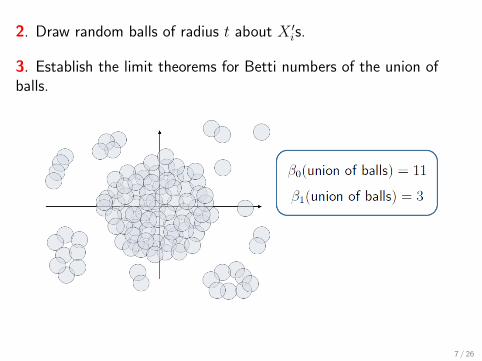
2. Draw random balls of radius t about X ′is.

3. Establish the limit theorems for Betti numbers of the union ofballs.

7 / 26

.Proposition [Adler et. al, 2014]...

.

. ..

.

.

There exists a sequence R(c)n = C ′(n/ log n)1/α for some C ′ > 0,

such that

P{B(0;R(c)

n ) ⊂∪

X∈Xn∩B(0;R(c)n )

B(X; 1)

}→ 1 , n → ∞,

where Xn = {X1, . . . , Xn}.

B(0;R(c)n ) is called a core.

8 / 26

The related notion, a weak core, plays a more decisive role in thecharacterization of the limit theorems.

.Definition..

.

. ..

.

.

Let f be a spherically symmetric density on Rd and R(w)n → ∞ be a

sequence determined by

nf(R(w)

n e1)→ 1 , n → ∞ .

Then B(0;R(w)n ) is called a weak core.

If f(x) = C/(1 + ||x||α

), x ∈ Rd, then R

(w)n = (Cn)1/α.

R(c)n /R

(w)n → 0, but they have the same regular variation

exponent, 1/α.

9 / 26

The related notion, a weak core, plays a more decisive role in thecharacterization of the limit theorems.

.Definition..

.

. ..

.

.

Let f be a spherically symmetric density on Rd and R(w)n → ∞ be a

sequence determined by

nf(R(w)

n e1)→ 1 , n → ∞ .

Then B(0;R(w)n ) is called a weak core.

If f(x) = C/(1 + ||x||α

), x ∈ Rd, then R

(w)n = (Cn)1/α.

R(c)n /R

(w)n → 0, but they have the same regular variation

exponent, 1/α.

9 / 26

Betti number in the tail

Xn = {X1, . . . , Xn}: iid Rd-valued random variables drawn froma power-law density with tail parameter α.

For k ≥ 1, define

βk,n(t) := βk

( ∪X∈Xn\B(0;Rn)

B(X; t)

), t ≥ 0 ,

where Rn is a non-random sequence with Rn ≥ R(w)n (= radius

of a weak core).

10 / 26

Betti number in the tail

Xn = {X1, . . . , Xn}: iid Rd-valued random variables drawn froma power-law density with tail parameter α.

For k ≥ 1, define

βk,n(t) := βk

( ∪X∈Xn\B(0;Rn)

B(X; t)

), t ≥ 0 ,

where Rn is a non-random sequence with Rn ≥ R(w)n (= radius

of a weak core).

10 / 26

Roughly speaking, as n → ∞, k-dim holes are distributed asfollows.

Three different regimes must be considered.We set, respectively,

I [1]: Rn = (Cn)1/(α−d/(k+2)),I [2]: (Cn)1/α ≪ Rn ≪ (Cn)1/(α−d/(k+2)),I [3]: Rn = (Cn)1/α,

and compute βk,n(t) by counting k-dim holes outside B(0;Rn).

11 / 26

Roughly speaking, as n → ∞, k-dim holes are distributed asfollows.

Three different regimes must be considered.We set, respectively,

I [1]: Rn = (Cn)1/(α−d/(k+2)),I [2]: (Cn)1/α ≪ Rn ≪ (Cn)1/(α−d/(k+2)),I [3]: Rn = (Cn)1/α,

and compute βk,n(t) by counting k-dim holes outside B(0;Rn).

11 / 26

In the regime [1],

There exist finitely many k-dim holes formed by k + 2 randompoints outside B(0;Rn) as n → ∞.

12 / 26

Example (k = 1)

The appearance of holes is a rare event.

13 / 26

Limiting process for βk,n(t):

Nk(t) :=

∫(Rd)k+1

ht(0, y1, . . . , yk+1)Mk(dy).

Mk is a Poisson random measure with Lebesgue intensitymeasure on (Rd)k+1.

ht(0, y1, . . . , yk+1) = 1

{βk

(B(0; t) ∪

∪k+1i=1 B(yi; t)

)= 1

}with 0, y1, . . . , yk+1 ∈ Rd.

14 / 26

ht(0,y) can be expressed as

ht(0,y) = h+t (0,y)− h−

t (0,y),

where h+t and h−

t are some other indicator functions, increasingin t.

Accordingly,

Nk(t) =

∫(Rd)k+1

h+t (0,y)Mk(dy)−

∫(Rd)k+1

h−t (0,y)Mk(dy)

:= N+k (t)−N−

k (t).

We can prove that N+k (t) and N−

k (t) are represented as a(time-changed) Poisson process.

I However, Nk(t) is not a (time-changed) Poisson process.

15 / 26

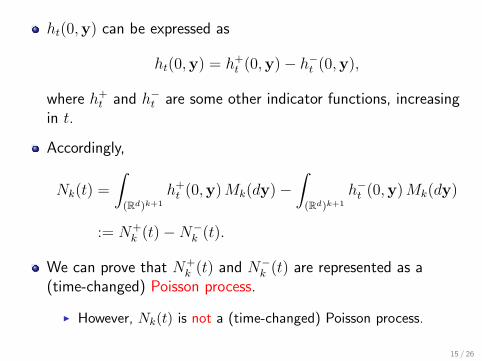
ht(0,y) can be expressed as

ht(0,y) = h+t (0,y)− h−

t (0,y),

where h+t and h−

t are some other indicator functions, increasingin t.

Accordingly,

Nk(t) =

∫(Rd)k+1

h+t (0,y)Mk(dy)−

∫(Rd)k+1

h−t (0,y)Mk(dy)

:= N+k (t)−N−

k (t).

We can prove that N+k (t) and N−

k (t) are represented as a(time-changed) Poisson process.

I However, Nk(t) is not a (time-changed) Poisson process.

15 / 26

.Theorem 1. [O., 2016]..

.

. ..

.

.

In the regime [1], we have, as n → ∞,

βk,n(t) ⇒ N+k (t)−N−

k (t).

16 / 26

In the regime [2],

There exist infinitely many k-dim holes formed by k + 2 pointsoutside B(0;Rn) as n → ∞.

17 / 26

Example (k = 1)

The appearance of holes is no longer a rare event.18 / 26

Limiting process for βk,n(t): Define a Gaussian process

Yk(t) :=

∫(Rd)k+1

ht(0, y1, . . . , yk+1)Gk(dy).

Gk is a Gaussian random measure with Lebesgue controlmeasure on (Rd)k+1.

ht(0, y1, . . . , yk+1) = 1

{βk

(B(0; t) ∪

∪k+1i=1 B(yi; t)

)= 1

}with 0, y1, . . . , yk+1 ∈ Rd.

19 / 26

Using the decomposition ht = h+t − h−

t , we can write

Yk(t) =

∫(Rd)k+1

h+t (0,y)Gk(dy)−

∫(Rd)k+1

h−t (0,y)Gk(dy)

:= Y +k (t)− Y −

k (t).

Then, Y +k (t) and Y −

k (t) are represented as a (time-changed)Brownian motion.

I Yk(t) is a Gaussian process, but it is not a (time-changed)Brownian motion.

20 / 26

.Theorem 2. [O., 2016]..

.

. ..

.

.

In the regime [2], we have, as n → ∞,

βk,n(t)− E{βk,n(t)

}(nk+2R

d−α(k+2)n

)1/2 ⇒ Y +k (t)− Y −

k (t).

21 / 26

In the regime [3],

22 / 26

Example (k = 1)

In the regimes [1] and [2], all the one-dim holes contributing toβ1,n(t) in the limit are always of the form

In the regime [3], many different kinds of one-dim holes (whichexist close enough to a weak core) contribute to β1,n(t) in thelimit.

23 / 26

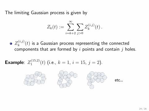
The limiting Gaussian process is given by

Zk(t) :=∞∑

i=k+2

∑j>0

Z(i,j)k (t) .

Z(i,j)k (t) is a Gaussian process representing the connected

components that are formed by i points and contain j holes.

Example: Z(15,2)1 (t) (i.e., k = 1, i = 15, j = 2).

24 / 26

The limiting Gaussian process is given by

Zk(t) :=∞∑

i=k+2

∑j>0

Z(i,j)k (t) .

Z(i,j)k (t) is a Gaussian process representing the connected

components that are formed by i points and contain j holes.

Example: Z(15,2)1 (t) (i.e., k = 1, i = 15, j = 2).

24 / 26

Rewrite Zk(t) as

Zk(t) = Z(k+2,1)k (t) +

∞∑i=k+3

∑j>0

Z(i,j)k (t) .

Z(k+2,1)k (t) represents the connected components that are

formed by k + 2 points and contain a single k-dimensional hole.

Example: Z(3,1)1 (t) (i.e., k = 1, i = 3, j = 1).

Z(k+2,1)k (t) is “similar” to the Yk(t) in the regime [2].

25 / 26

Rewrite Zk(t) as

Zk(t) = Z(k+2,1)k (t) +

∞∑i=k+3

∑j>0

Z(i,j)k (t) .

Z(k+2,1)k (t) represents the connected components that are

formed by k + 2 points and contain a single k-dimensional hole.

Example: Z(3,1)1 (t) (i.e., k = 1, i = 3, j = 1).

Z(k+2,1)k (t) is “similar” to the Yk(t) in the regime [2].

25 / 26

.Theorem 3. [O., 2016]..

.

. ..

.

.

In the regime [3], we have, as n → ∞,

βk,n(t)− E{βk,n(t)

}nd/(2α)

⇒ Zk(t).

26 / 26