Likelihood Analysis of the pMSSM11 in Light of LHC 13-TeV Data

Likelihood Analysis of the pMSSM11 in Light of

LHC 13-TeV DataE. Bagnaschia, K. Sakuraib, M. Borsatoc, O. Buchmuellerd, M. Citrond, J. C. Costad,A. De Roecke, M.J. Dolanf , J.R. Ellisg, H. Flacherh, S. Heinemeyeri, M. Lucioc,D. Martınez Santosc, K.A. Olivej, A. Richardsd, V.C. Spanosk, I. Suarez Fernandezc,G. Weigleina

aDESY, Notkestraße 85, D–22607 Hamburg, Germany

bInstitute of Theoretical Physics, Faculty of Physics, University of Warsaw, ul. Pasteura 5, PL–02–093Warsaw, Poland

cInstituto Galego de Fısica de Altas Enerxıas, Universidade de Santiago de Compostela, Spain

dHigh Energy Physics Group, Blackett Laboratory, Imperial College, Prince Consort Road, London SW7 2AZ, UK

eExperimental Physics Department, CERN, CH–1211 Geneva 23, Switzerland;Antwerp University, B–2610 Wilrijk, Belgium

fARC Centre of Excellence for Particle Physics at the Terascale, School of Physics, University ofMelbourne, 3010, Australia

gTheoretical Particle Physics and Cosmology Group, Department of Physics, King’s College London,London WC2R 2LS, UK;National Institute of Chemical Physics and Biophysics, Ravala 10, 10143 Tallinn, Estonia;Theoretical Physics Department, CERN, CH–1211 Geneva 23, Switzerland

hH.H. Wills Physics Laboratory, University of Bristol, Tyndall Avenue, Bristol BS8 1TL, UK

iCampus of International Excellence UAM+CSIC, Cantoblanco, E–28049 Madrid, Spain;Instituto de Fısica Teorica UAM-CSIC, C/ Nicolas Cabrera 13-15, E–28049 Madrid, Spain;Instituto de Fısica de Cantabria (CSIC-UC), Avda. de Los Castros s/n, E–39005 Santander, Spain

jWilliam I. Fine Theoretical Physics Institute, School of Physics and Astronomy, University ofMinnesota, Minneapolis, Minnesota 55455, USA

kSection of Nuclear & Particle Physics, Department of Physics, National and Kapodistrian Universityof Athens, GR15784 Athens, Greece

We use MasterCode to perform a frequentist analysis of the constraints on a phenomenological MSSM modelwith 11 parameters, the pMSSM11, including constraints from ∼ 36/fb of LHC data at 13 TeV and PICO,XENON1T and PandaX-II searches for dark matter scattering, as well as previous accelerator and astrophysicalmeasurements, presenting fits both with and without the (g − 2)µ constraint. The pMSSM11 is specified by thefollowing parameters: 3 gaugino masses M1,2,3, a common mass for the first-and second-generation squarks mq anda distinct third-generation squark mass mq3 , a common mass for the first-and second-generation sleptons m˜ anda distinct third-generation slepton mass mτ , a common trilinear mixing parameter A, the Higgs mixing parameterµ, the pseudoscalar Higgs mass MA and tanβ. In the fit including (g − 2)µ, a Bino-like χ0

1 is preferred, whereasa Higgsino-like χ0

1 is mildly favoured when the (g − 2)µ constraint is dropped. We identify the mechanisms thatoperate in different regions of the pMSSM11 parameter space to bring the relic density of the lightest neutralino,χ0

1, into the range indicated by cosmological data. In the fit including (g − 2)µ, coannihilations with χ02 and the

Wino-like χ±1 or with nearly-degenerate first- and second-generation sleptons are active, whereas coannihilationswith the χ0

2 and the Higgsino-like χ±1 or with first- and second-generation squarks may be important when the(g − 2)µ constraint is dropped. In the two cases, we present χ2 functions in two-dimensional mass planes aswell as their one-dimensional profile projections and best-fit spectra. Prospects remain for discovering strongly-interacting sparticles at the LHC, in both the scenarios with and without the (g − 2)µ constraint, as well as fordiscovering electroweakly-interacting sparticles at a future linear e+e− collider such as the ILC or CLIC.

KCL-PH-TH/2017-22, CERN-PH-TH/2017-087, DESY 17-059, IFT-UAM/CSIC-17-035

FTPI-MINN-17/17, UMN-TH-3701/17

arX

iv:1

710.

1109

1v3

[he

p-ph

] 1

May

201

8

1. Introduction

Supersymmetric (SUSY) models of TeV-scalephysics are being subjected to increasing pressureby the strengthening constraints imposed by LHCexperiments [1, 2] and searches for Dark Matter(DM) [3–6]. In particular, in the context of mod-els with soft supersymmetry-breaking parametersconstrained to be universal at a high unifica-tion scale, the LHC limits on sparticle masseshave been in increasing tension with a super-symmetric interpretation of the anomalous mag-netic moment of the muon, (g−2)µ, which wouldrequire relatively light sleptons and electroweakgauginos [7–10]. This pressure has been ratch-eted up by the advent of ∼ 36/fb of data fromRun 2 of the LHC at a centre-of-mass energy of13 TeV [11–13] 1, which probe supersymmetricmodels at significantly higher mass scales thanwas possible in Run 1 at 7 and 8 TeV in thecentre of mass. In parallel, direct searches forDM scattering have also been making significantprogress towards the neutrino ‘floor’ [14], in par-ticular with the recent data releases from theLUX, PICO, XENON1T and PandaX-II exper-iments [3–6]. Here we analyze these constraintsin the minimal supersymmetric extension of theStandard Model (MSSM), which, because of R-parity, has a stable cosmological relic particle thatwe assume to be the lightest neutralino, χ0

1, [15].The strengthening phenomenological, experi-

mental and astrophysical constraints on super-symmetry (SUSY) were initially explored mainlyin the contexts of models in which SUSY breakingwas assumed to be universal at the GUT scale,such as the constrained MSSM (CMSSM) [7, 8,16], non-universal Higgs models (NUHM1,2) [8,9] 2, the minimal anomaly-mediated SUSY-breaking model (mAMSB) [18], and models basedon the SU(5) group [19]. These models aretractable by virtue of having a relatively limited

1We use here results from SUSY searches by the CMSCollaboration: the results from ATLAS [2] yield similarconstraints.2For a recent analysis of these models in light of ∼ 13/fbof LHC data at 13 TeV, see [17]. This analysis does notinclude the PICO, XENON1T and most recent PandaX-IIresults, and has other differences that are noted later inthis paper.

number of parameters, though the universality as-sumptions they employ are not necessarily wellsupported in scenarios motivated by fundamen-tal principles, such as string theory. Their limitedparameter spaces are amenable to analysis, e.g.,in the frequentist approach we follow, in whichone constructs a global likelihood function thatembodies all the information provided by the mul-tiple constraints.

Alternatively, one may study phenomenolog-ical models in which the soft SUSY-breakingparameters are not constrained by any univer-sality assumptions, though subject to milderconstraints emanating, in particular, from up-per limits on SUSY contributions to flavour-changing processes. These phenomenologicalMSSM (pMSSM) [20] models contain many moreparameters, whose exploration is computationallydemanding. There have been cut-based globalanalyses of variants of the pMSSM with as manyas 19 parameters [21] and global fits focused onspecific sectors or parameter ranges [22], how-ever in the past we have restricted our frequen-tist attentions to a variant of the pMSSM with10 parameters, the pMSSM10 [10,23]. These weretaken to be 3 independent gaugino masses, M1,2,3,a common electroweak-scale mass for the first-andsecond-generation squarks, mq, a distinct massfor the third-generation squarks, mq3 , a commonelectroweak-scale mass ml for the sleptons, a sin-gle trilinear mixing parameter A that is universalat the electroweak scale, the Higgs mixing param-eter µ, the pseudoscalar Higgs mass, MA and theratio of Higgs vevs, tanβ 3.

It is desirable to extend this type of analysis tomore general variants of the pMSSM, for a coupleof reasons. One is that the lower bounds on spar-ticle masses will, in general, be weaker in modelswith more parameters, so one should explore suchmodels before making statements about the mag-nitudes of these lower bounds and prospects fordiscovering sparticles at the LHC or elsewhere.Another reason is that reconciling the strength-ening LHC constraints with the cosmological DMdensity constraint requires, in general, specific

3For a recent analysis of a 7-dimensional version of theMSSM in light of ∼ 13/fb of LHC data at 13 TeV, see [24].

2

3

relations between sparticle masses that suppressthe relic density via coannihilation effects and/orrapid annihilations through direct-channel reso-nances. Therefore one should study models capa-ble of accommodating these DM mechanisms [23].

Examples of DM mechanisms that have beenstudied extensively in the past [23] include coan-nihilation with the lighter stau slepton, τ1, thelighter chargino, χ±1 , or the lighter stop squark,t1, and rapid annihilations via the Z boson, the125-GeV Higgs boson, h, or the heavier MSSMHiggs bosons, H/A. More recently, the possibil-ity of coannihilation with gluinos, g, has beenexplored in models with non-universal gauginomasses [25,26], and coannihilation with the right-handed up-type squarks of the first two genera-tions, uR/cR, emerged as a possibility in an SU(5)model with non-universal scalar masses m5,m10

for sfermions in 5 and 10 representations [19].All of these were possibilities in the pMSSM10,

but in that scenario the stau and smuon masseswere fixed to be equal, putting the LHC con-straints on stau coannihilation in tension with thepossibility of a SUSY interpretation of (g−2)µ, atension that has increased with the advent of thefirst LHC data at 13 TeV. In this paper we studytwo possible resolutions of this issue. We study anextension of the parameter space of the pMSSM10to 11 parameters by relaxing the equality betweenthe soft SUSY-breaking contributions to the staumass and to the (still common) masses of thesmuon and selectron, the pMSSM11. In order toassess the importance of the (g − 2)µ constraint,we also consider a fit omitting the SUSY inter-pretation of (g−2)µ. The principal results of thispaper are comparisons between the likelihoods ofdifferent spectra in the pMSSM11 with and with-out (g− 2)µ, and comparisons between the likeli-

hoods of different DM mechanisms including τ1, ˜,q and g coannihilation, highlighting the impactsof the LHC 13 TeV and recent DM scatteringdata.

The layout of this paper is as follows. InSect. 2 we specify the framework of our analy-sis. Subsection 2.1 specifies the pMSSM11, es-tablishes our notation for its parameters and de-scribes our procedure for sampling the pMSSM11

parameter space. In Subsection 2.2 we review theMasterCode tool to construct a global χ2 like-lihood function combining constraints on modelparameters, Subsection 2.3 describes our treat-ments of the electroweak and flavour constraints,including some updates compared with our pre-vious analyses. In Subsection 2.4 we give detailson our DM analysis, which includes constraintson both spin-independent and -dependent DMscattering [3–6]. Our implementations of the con-straints from ∼ 36/fb of LHC at 13 TeV [11–13]are discussed in Subsection 2.5. Then, in Sec-tion 3.1 we present results for the global likelihoodfunction in various parameter planes, highlight-ing the regions where different DM mechanismsoperate and comparing results with and withoutthe (g − 2)µ constraint being applied. Section 4displays the one-dimensional profile likelihoodfunctions for various masses, mass differencesand other observables in these two cases, andalso shows predictions for spin-independent and -dependent DM scattering. Section 5 highlightsthe impacts of the LHC 13-TeV data [11–13]and the recent direct searches for astrophysicalDM [3–6]. Section 6 discusses the best-fit points,favoured and allowed spectra in these pMSSMscenarios. Finally, Section 7 summarizes our con-clusions.

2. Analysis Framework

2.1. Model ParametersAs mentioned above, in this paper we con-

sider a pMSSM scenario with eleven parameters,namely

3 gaugino masses : M1,2,3 ,

2 squark masses : mq ≡mq1 ,mq2

6= mq3 = mt,mb,

2 slepton masses : m˜ ≡ m˜1

= m˜2

= me,mµ

6= m`3 = mτ ,

1 trilinear coupling : A , (1)

Higgs mixing parameter : µ ,

pseudoscalar Higgs mass : MA ,

ratio of vevs : tanβ ,

4

where q1,2 ≡ u, d, s, c, we assume soft SUSY-breaking parameters for left- and right-handedsfermions, and the sneutrinos have the same softSUSY-breaking parameter as the correspondingcharged sfermions. All of these parameters arespecified at a renormalisation scale MSUSY givenby the geometric mean of the masses of the scalartop eigenstates, MSUSY ≡ √mt1

mt2, which is also

the scale at which electroweak symmetry break-ing conditions are imposed. We allow the signof the mixing parameter µ to be either positiveor negative. The important difference from thepMSSM10 scenario we studied previously [10] isthat the first- and second-generation slepton massm˜ and the stau mass mτ are decoupled in thepMSSM11 4.

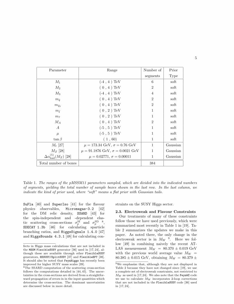
The ranges of these parameters sampled in ouranalysis are displayed in Table 1. In each case, weindicate in the third column of Table 1 how theranges of most of these parameters are dividedinto segments, much as we did previously for ouranalysis of the pMSSM10 [10].

These segments define boxes in the eleven-dimensional parameter space, which we sampleusing the MultiNest package [29]. In order toensure a smooth overlap between boxes and elim-inate features associated with their boundaries,we choose for each box a prior such that 80% ofthe sample has a flat distribution within the nom-inal box, and 20% of the sample is in normally-distributed tails extending outside the box. Aninitial scan over all mass parameters with abso-lute values ≤ 4 TeV showed that non-trivial be-haviour of the global likelihood function was re-stricted to |M1| . 1 TeV and m˜ . 1 TeV. Inorder to achieve high resolution efficiently, we re-stricted the range of m˜ to < 2 TeV in the fullscan 5. To study properly the impact of the(g − 2)µ, we performed separate sampling cam-paigns with and without it. On the other hand,during the sampling phase the constraints com-

4In comparison, the pMSSM7 scenario studied in [24] as-sumes gaugino and squark/slepton mass universality atsome input scale Q, and has two trilinear couplings At,b,independent Higgs masses Hu,d and tanβ as free param-eters.5Since m˜ > mχ0

1, this entails also the restriction to

mχ01< 2 TeV visible in subsequent figures.

ing from LHC13 results have not been included.Since their impact consists in providing lowerbounds to the sparticle masses, this choice al-lows for a proper assessment of their impact onthe full parameter space. Moreover, we also per-formed dedicated scans for various DM annihi-lation mechanisms, in such a way to improve thequality of the sample in the description of the fine-tuned spectrum configurations that characterizethem. The data sets from the various campaignshave been merged into a single set on which thelikelihood is computed dynamically including orexcluding the (g − 2)µ and/or the LHC13 con-straints according to our interest. The total num-ber of points in our pMSSM11 parameter scan is∼ 2× 109.

2.2. MasterCodeWe perform a global likelihood analysis of

the pMSSM11 including constraints from directsearches for SUSY particles at the LHC, mea-surements of the Higgs boson mass and signalstrengths, LHC searches for SUSY Higgs bosons,precision electroweak observables, flavour con-straints from B- and K-physics observables, thecosmological constraint on the overall cold darkmatter (CDM) density, and upper limits on spin-independent and -dependent LSP-nuclear scatter-ing. We treat (g − 2)µ as an optional constraint,presenting results from global fits with and with-out it, and we treat mt, αs and MZ as nuisanceparameters.

The observables contributing to the like-lihood are calculated using the MasterCode

tool [7–10, 18, 19, 23, 30], which interfaces andcombines consistently various public and pri-vate codes using the SUSY Les Houches Ac-cord (SLHA) [31]. The following codes are usedin this analysis: SoftSusy 3.3.9 [32] for thespectrum, FeynWZ [33] for the electroweak pre-cision observables 6, FeynHiggs 2.11.3 [35]for the Higgs sector 7 and (g − 2)µ,

6We use here an updated version of FeynWZ (not yet pub-licly available) in which theMW evaluation is based on [34]and is identical to that implemented in FeynHiggs, whichgives more reliable results in parameter regions with largerSUSY masses or small SUSY mass splittings. The otherEWPO are treated in the same way as in [33].7We note that FeynHiggs incorporates resummation ef-

5

Parameter Range Number of Prior

segments Type

M1 (-4 , 4 ) TeV 6 soft

M2 ( 0 , 4 ) TeV 2 soft

M3 (-4 , 4 ) TeV 4 soft

mq ( 0 , 4 ) TeV 2 soft

mq3 ( 0 , 4 ) TeV 2 soft

m˜ ( 0 , 2 ) TeV 1 soft

mτ ( 0 , 2 ) TeV 1 soft

MA ( 0 , 4 ) TeV 2 soft

A (-5 , 5 ) TeV 1 soft

µ (-5 , 5 ) TeV 1 soft

tanβ ( 1 , 60) 1 soft

Mt [27] µ = 173.34 GeV, σ = 0.76 GeV 1 Gaussian

MZ [28] µ = 91.1876 GeV, σ = 0.0021 GeV 1 Gaussian

∆α(5)had(MZ) [28] µ = 0.02771, σ = 0.00011 1 Gaussian

Total number of boxes 384

Table 1. The ranges of the pMSSM11 parameters sampled, which are divided into the indicated numbersof segments, yielding the total number of sample boxes shown in the last row. In the last column, weindicate the kind of prior used, where “soft” means a flat prior with Gaussian tails.

SuFla [40] and SuperIso [41] for the flavourphysics observables, Micromegas-3.2 [42]for the DM relic density, SSARD [43] forthe spin-independent and -dependent elas-tic scattering cross-sections σSI

p and σSDp

8,SDECAY 1.3b [46] for calculating sparticlebranching ratios, and HiggsSignals 1.4.0 [47]and HiggsBounds 4.3.1 [48] for calculating con-

fects in Higgs mass calculations that are not included inthe MSSM FlexibleSUSY generator [36] used in [17, 24], al-though these are available through other FlexibleSUSY

generators, HSSUSY/SplitSUSY [37] and FlexibleEFT [38].It should also be noted that FeynHiggs has recently beenimproved for higher SUSY mass scales [39].8The SSARD computation of the scattering cross-sectionfollows the computations detailed in [44, 45]. The uncer-tainties in the cross-sections are derived from a straightfor-ward propagation of errors in in the input quantities whichdetermine the cross-section. The dominant uncertaintiesare discussed below in more detail.

straints on the SUSY Higgs sector.

2.3. Electroweak and Flavour ConstraintsOur treatments of many of these constraints

follow those we have used previously, which weresummarized most recently in Table 1 in [19]. Ta-ble 2 summarizes the updates we make in thispaper. As noted there, the only change in theelectroweak sector is in MW

9. Here we fol-low [49] in combining naively the recent AT-LAS measurement MW = 80.370 ± 0.019 GeVwith the previous world average value MW =80.385 ± 0.015 GeV, obtaining MW = 80.379 ±9We emphasize that, although they are not displayed inTable 2 because they have not changed since [19], we usea complete set of electroweak constraints, not restricted toMW as used in [17,24]. We also note that the FeynWZ codewe use to calculate MW incorporates 2-loop correctionsthat are not included in the FlexibleSUSY code [36] usedin [17,24].

6

0.012 GeV 10.Since one of our objectives in this paper is to

emphasize the impact on the pMSSM11 parame-ter space of the (g − 2)µ constraint, for referencewe also include in Table 2 the implementation ofthis constraint that we use as an option 11

As can be seen in Table 2, we have also up-dated a number of flavour constraints. In par-ticular, we have updated the global analysis ofBR(Bs,d → µ+µ−) to include the latest Run 2result from LHCb [57] as well as the Run 1 resultsof CMS, LHCb [55] and ATLAS [56]. We assumeminimal flavour violation (MFV) when combin-ing the BR(Bd → µ+µ−) constraint with thatfrom BR(Bs → µ+µ−) into the quantity Rµµ [8],and take into account the correlation between thetheoretical calculations of fBs and fBd

.The LHCb Collaboration has also pub-

lished [57] a first determination of the effectiveBs lifetime as measured in Bs → µ+µ− decays,providing a constraint on the quantity A∆Γ viathe relation

τ(Bs → µ+µ−)

τ(Bs → µ+µ−)|SM=

1 + 2A∆Γys + y2s

(1 + ys)(1 +A∆Γys),

(2)

where [59]

ys = τBs

∆Γs2

= 0.0675± 0.004 ,

A∆Γ ≡ −2Re(λ)

(1 + |λ|2), (3)

λ ≡ q

p

A(Bs → µ+µ−)

A(Bs → µ+µ−),

where τBsis the inclusive Bs decay lifetime, the

complex numbers p, q specify the relation betweenthe mass eigenstates of the B0

s − B0s system and

the flavour eigenstates [59], and A(B0s → µ+µ−)

10In so doing, we neglect correlations in the uncertain-ties due to PDFs, QED and boson pT modelling, but ourresults are relatively insensitive to the details of this com-bination.11The (g − 2)µ evaluation in FeynHiggs contains less so-phisticated two-loop corrections than GM2CALC [50]. How-ever, the difference is small compared with other uncer-tainties in our analysis.

and A(B0s → µ+µ−) are the B0

s and B0s de-

cay amplitudes. In the Standard Model (SM),A∆Γ = 1 so that τ(Bs → µ+µ−)|SM = τBs

/(1 −ys) = 1.619 ± 0.009 ps. On general grounds,A∆Γ ∈ [−1, 1]. The LHCb measurement τ(Bs →µ+µ−) = 2.04 ± 0.44(stat.) ± 0.05(syst.) ps cor-responds formally to A∆Γ = 7.7± 10.0, implyingthat the current LHCb result does not constrainsignificantly the pMSSM11 parameter space, andwe do not include it in our fit. However, in thelater discussion of our fit results we present forinformation the χ2 profile likelihood functions wefind for A∆Γ and τ(Bs → µ+µ−).

We have also updated our implementations ofb → sγ, B → τν, B → Xs``, ∆MBs

and ∆MBd

to take account of updated theoretical calcula-tions within the SM. For the same reason, in thekaon sector we have also updated our implemen-tations of K → µν and K → πνν 12. Since thereare, in general, supersymmetric contributions tothe observables commonly used in global fits toCKM parameters, we remove these contributionsand make a global fit to the CKM parameterswithout them.

In general, we treat the electroweak precisionobservables, (g − 2)µ and all B- and K-physicsobservables (except for BR(Bs,d → µ+µ−)) asGaussian constraints, combining in quadraturethe experimental and applicable SM and SUSYtheory errors.

2.4. Dark Matter Constraints andMechanisms

Cosmological densitySince we work in the framework of the MSSM,R-parity is conserved, so that the lightestSUSY particle (LSP) is a candidate to pro-vide the CDM. We assume that the LSP isthe lightest neutralino χ0

1 [15], and that it isthe dominant component of the CDM. As inour recent papers [18, 19], we use the Planck2015 constraint on the total CDM density:ΩCDMh

2 = 0.1186± 0.0020EXP ± 0.0024TH [73].

Density mechanismsAs one of the primary objectives in our analysis

12We refer to Table 1 of [19] for a complete set of theK-decay constraints we implement.

7

Observable Source Constraint

Th./Ex.

MW [GeV] [33] / [51,52] 80.379± 0.012± 0.010MSSM

aEXPµ − aSM

µ [53] / [54] (30.2± 8.8± 2.0MSSM)× 10−10

Rµµ [55–57] 2D likelihood, MFV

τ(Bs → µ+µ−) [57] 2.04± 0.44(stat.)± 0.05(syst.) ps

BREXP/SMb→sγ [58]/ [59] 0.988± 0.045EXP ± 0.068TH,SM ± 0.050TH,SUSY

BREXP/SMB→τν [59, 60] 0.883± 0.158EXP ± 0.096SM

BREXP/SMB→Xs``

[61]/ [59] 0.966± 0.278EXP ± 0.037SM

∆MEXP/SMBs

[40, 62] / [59] 0.968± 0.001EXP ± 0.078SM

∆MEXP/SMBs

∆MEXP/SMBd

[40, 62] / [59] 1.007± 0.004EXP ± 0.116SM

BREXP/SMK→µν [40, 63] / [64] 1.0005± 0.0017EXP ± 0.0093TH

BREXP/SMK→πνν [65]/ [66] 2.01± 1.30EXP ± 0.18SM

σSIp [3, 4, 6] Combined likelihood in the (mχ0

1, σSIp ) plane

σSDp [5] Likelihood in the (mχ0

1, σSDp ) plane

g → qqχ01, bbχ

01, ttχ

01 [11, 12] Combined likelihood in the (mg,mχ0

1) plane

q → qχ01 [11] Likelihood in the (mq,mχ0

1) plane

b→ bχ01 [11] Likelihood in the (mb,mχ0

1), plane

t1 → tχ01, cχ

01, bχ

±1 [11] Likelihood in the (mt1

,mχ01), plane

χ±1 → ν`±χ01, ντ

±χ01,W

±χ01 [13] Likelihood in the (m

χ±1,mχ0

1) plane

χ02 → `+`−χ0

1, τ+τ−χ0

1, Zχ01 [13] Likelihood in the (mχ0

2,mχ0

1) plane

Heavy stable charged particles [67] Fast simulation based on [67,68]

H/A→ τ+τ− [69–72] Likelihood in the (MA, tanβ) plane

Table 2Experimental constraints that we update in this work compared to Table 1 in [19]. We indicate separatelythe experimental and applicable theoretical errors in the SM and SUSY (sometimes in combination, la-belled “MSSM”). The contribution of the τ(Bs → µ+µ−) constraint to the global χ2 likelihood function isessentially constant across the relevant region of the pMSSM11 parameter space, and it is not includedin the fit. The new LHC constraints are all based on ∼ 36/fb of data at 13 TeV.

is to investigate the relevances of various mech-anisms for bringing the relic χ0

1 density into therange allowed by astrophysics and cosmology, weintroduce a set of measures related to particlemasses that were found in our previous anal-yses [23] to indicate when specific mechanismswere dominant 13. These may be grouped as

13We have checked specifically the validity of these mea-sures using Micromegas, finding good consistency in mostcases. However, in certain hybrid regions where more than

follows.

•Coannihilation with an InoThis may be important if the χ0

1 is not muchlighter than the lighter chargino, χ±1 , and the sec-ond neutralino, χ0

2, or the gluino, g. For these

one mechanism satisfied the criteria we found that just onemechanism dominates. Moreover, it might also happenthat some regions of the parameter space are not classifiedby a given measure even if the corresponding mechanismis active.

8

cases we introduce the coannihilation measures

Ino coann. :

(MIno

mχ01

− 1

)< 0.25 . (4)

We find that chargino and χ02 coannihilation is im-

portant in our analysis, and in our 2-dimensionalplots we shade green the regions where (4) issatisfied when the Ino is the lighter chargino, χ±1(which is almost degenerate with the χ0

2). Onthe other hand, we find that gluino coannihila-tion is not important in the pMSSM11 when the(g − 2)µ constraint is imposed. This is due tothe fact that (g − 2)µ forces the neutralino massto values for which a gluino of equivalent masswould be excluded by current LHC results.

•Coannihilation with sleptonsIn the version of the pMSSM that we study

here, the two stau mass eigenvalues are simi-lar, since the soft SUSY-breaking parameters arespecified at the TeV scale and the left-right mix-ing ∝ mτ is relatively small, but the stau massesare not degenerate with the selectron and smuonmasses, in general. We find that smuon and selec-tron coannihilation are in general more importantthan stau coannihilation, thanks to the greatermultiplicity of near-degenerate states. We intro-duce the following coannihilation measure:

˜ coann. :

(m˜

mχ01

− 1

)< 0.15 , (5)

and shade in yellow (pink) the regions of ourtwo-dimensional plots where (5) is satisfied for` = µ, e (τ), respectively.

•Coannihilation with squarksSimilarly, this may be important for squarks q

that are not much heavier than the χ01. The case

considered most often has been q = t1, but herewe consider all possibilities, including coannihi-lations with first- and second-generation squarks,which we find to be important when the LHC13-TeV constraint or (g − 2)µ is dropped. Weintroduce the coannihilation measure

q coann. :

(mq

mχ01

− 1

)< 0.15 , (6)

and we use the following colours in our plots forthe regions where (6) is satisfied: q = d/s/u/cL,Rcyan, t1 grey, b1 purple.

•Annihilation via a direct-channel boson poleWhen there is a massive boson B with mass

MB ∼ 2mχ01, χ0

1χ01 annihilation is enhanced along

a ‘funnel’ in parameter space. We have foundthat such a mechanism is likely to dominate ifthe following condition is satisfied:

B funnel :

∣∣∣∣∣MB

mχ01

− 2

∣∣∣∣∣ < 0.1 . (7)

We have considered the cases B = h, Z and H/A,and use blue shading for the regions of our subse-quent plots where (7) is satisfied when B = H/A.We comment later on a small region where rapidannihilation via the h and Z poles is important.

•Enhanced Higgsino componentWe have also considered a somewhat different

possibility, namely that the χ01 has an enhanced

Higgsino component because the following condi-tion is satisfied, which is similar to the situationin the focus-point region of the CMSSM:

Higgsino :

∣∣∣∣∣

(µ

mχ01

)− 1

∣∣∣∣∣ < 0.3 . (8)

Regions where the condition (8) is satisfied gener-ally satisfy the chargino coannihilation conditionwith a Higgsino-like LSP, and are also shadedgreen.

•Hybrid regionsIn addition to the ‘primary’ regions where only

one of the conditions (4, 5, 6, 7, 8) is satisfied,there are also ‘hybrid’ regions where more thanone condition is satisfied. These are indicated inthe following by mixtures of the correspondingprimary colours.

Direct DM searchesWe implement experimental constraints from di-rect searches for supersymmetric DM via bothspin-independent and -dependent scattering onnuclei. We use the LUX [4], XENON1T [6]

9

and PandaX-II [3] constraints on the spin-independent DM scattering cross section σSI

p ,which we implement via a combined two-dimensional likelihood function in the (mχ0

1, σSIp )

plane.Our treatment of the spin-independent nuclear

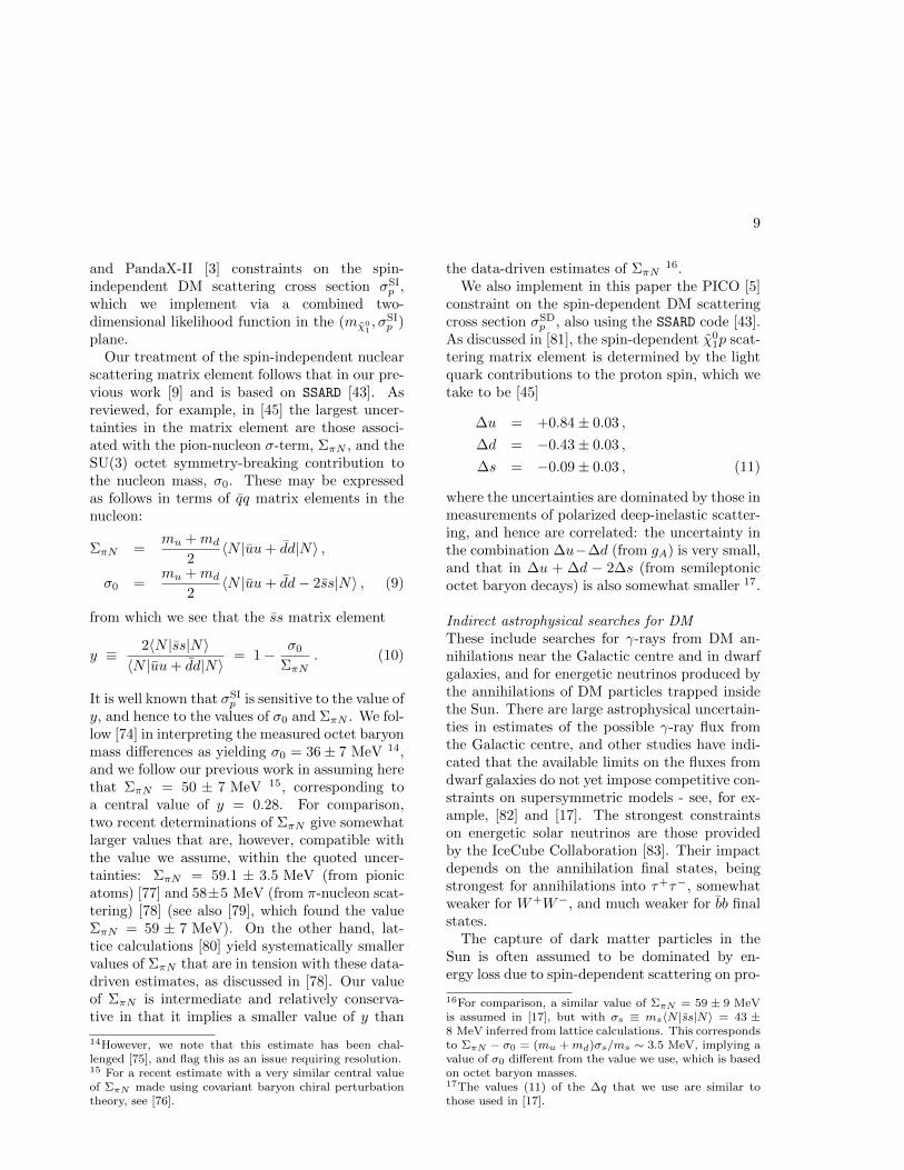
scattering matrix element follows that in our pre-vious work [9] and is based on SSARD [43]. Asreviewed, for example, in [45] the largest uncer-tainties in the matrix element are those associ-ated with the pion-nucleon σ-term, ΣπN , and theSU(3) octet symmetry-breaking contribution tothe nucleon mass, σ0. These may be expressedas follows in terms of qq matrix elements in thenucleon:

ΣπN =mu +md

2〈N |uu+ dd|N〉 ,

σ0 =mu +md

2〈N |uu+ dd− 2ss|N〉 , (9)

from which we see that the ss matrix element

y ≡ 2〈N |ss|N〉〈N |uu+ dd|N〉 = 1− σ0

ΣπN. (10)

It is well known that σSIp is sensitive to the value of

y, and hence to the values of σ0 and ΣπN . We fol-low [74] in interpreting the measured octet baryonmass differences as yielding σ0 = 36± 7 MeV 14,and we follow our previous work in assuming herethat ΣπN = 50 ± 7 MeV 15, corresponding toa central value of y = 0.28. For comparison,two recent determinations of ΣπN give somewhatlarger values that are, however, compatible withthe value we assume, within the quoted uncer-tainties: ΣπN = 59.1 ± 3.5 MeV (from pionicatoms) [77] and 58±5 MeV (from π-nucleon scat-tering) [78] (see also [79], which found the valueΣπN = 59 ± 7 MeV). On the other hand, lat-tice calculations [80] yield systematically smallervalues of ΣπN that are in tension with these data-driven estimates, as discussed in [78]. Our valueof ΣπN is intermediate and relatively conserva-tive in that it implies a smaller value of y than

14However, we note that this estimate has been chal-lenged [75], and flag this as an issue requiring resolution.15 For a recent estimate with a very similar central valueof ΣπN made using covariant baryon chiral perturbationtheory, see [76].

the data-driven estimates of ΣπN16.

We also implement in this paper the PICO [5]constraint on the spin-dependent DM scatteringcross section σSD

p , also using the SSARD code [43].As discussed in [81], the spin-dependent χ0

1p scat-tering matrix element is determined by the lightquark contributions to the proton spin, which wetake to be [45]

∆u = +0.84± 0.03 ,

∆d = −0.43± 0.03 ,

∆s = −0.09± 0.03 , (11)

where the uncertainties are dominated by those inmeasurements of polarized deep-inelastic scatter-ing, and hence are correlated: the uncertainty inthe combination ∆u−∆d (from gA) is very small,and that in ∆u + ∆d − 2∆s (from semileptonicoctet baryon decays) is also somewhat smaller 17.

Indirect astrophysical searches for DMThese include searches for γ-rays from DM an-nihilations near the Galactic centre and in dwarfgalaxies, and for energetic neutrinos produced bythe annihilations of DM particles trapped insidethe Sun. There are large astrophysical uncertain-ties in estimates of the possible γ-ray flux fromthe Galactic centre, and other studies have indi-cated that the available limits on the fluxes fromdwarf galaxies do not yet impose competitive con-straints on supersymmetric models - see, for ex-ample, [82] and [17]. The strongest constraintson energetic solar neutrinos are those providedby the IceCube Collaboration [83]. Their impactdepends on the annihilation final states, beingstrongest for annihilations into τ+τ−, somewhatweaker for W+W−, and much weaker for bb finalstates.

The capture of dark matter particles in theSun is often assumed to be dominated by en-ergy loss due to spin-dependent scattering on pro-

16For comparison, a similar value of ΣπN = 59 ± 9 MeVis assumed in [17], but with σs ≡ ms〈N |ss|N〉 = 43 ±8 MeV inferred from lattice calculations. This correspondsto ΣπN − σ0 = (mu +md)σs/ms ∼ 3.5 MeV, implying avalue of σ0 different from the value we use, which is basedon octet baryon masses.17The values (11) of the ∆q that we use are similar tothose used in [17].

10

tons, in which case an upper limit on the neutrinoflux may be used to constrain the spin-dependentcross-section σSD

p , as done by the IceCube Col-laboration [83]. However, the interpretation ofthis constraint [83] depends on the importance ofspin-independent scattering on 4He and heaviernuclei inside the Sun, and whether the DM den-sity inside the Sun is in equilibrium between cap-ture and annihilation [84]. As discussed in Sec-tion 4.10, we have found in an exploratory studythat the IceCube constraint has little impact oncethe more recent PICO constraint [5] on σSD

p istaken into account. In view of the fact that it hasfewer uncertainties, we use the PICO result in ourglobal fit, setting aside the IceCube result [83] 18.

2.5. 13 TeV LHC ConstraintsThe LHC constraints we consider are those

from searches for coloured sparticles in eventswith missing transverse energy, /ET , accompa-nied by jets and possibly leptons, searches forelectroweak inos in events with multiple lep-tons, searches for long-lived charged particles,measurements of the 125 GeV Higgs boson h,and searches for the heavier SUSY Higgs bosonsH,A,H±. Our principal focus in this paperis on the implications of Run-2 LHC searcheswith ∼ 36/fb of data at 13 TeV, though wealso make comparisons with the situation beforethese constraints were released. Our implemen-tations of the constraints from LHC Run 1 atenergies of 7 and 8 TeV used in our previousanalysis of the pMSSM10 model were describedin [10], and our implementations of /ET searcheswith ∼ 13/fb of data at 13 TeV in the gluinoand squark production channels were describedin [19], as were our implementations of searchesfor long-lived charged particles and for H,A,H±

with similar data sets. We refer the reader tothese publications for details of those implemen-tations, focusing here on our implementations ofthe Run 2 searches with ∼ 36/fb of data.

Searches for gluinos and squarksWe consider the constraints from CMS simpli-

fied model searches using events with /ET and jets

18In contrast, [17] uses the IceCube result, but not thePICO result.

but no leptons released in [11] and events with /ETand jets and a single lepton released in [12].

In the approach taken, e.g., by CheckMATE

[85], ColliderBit [86] and MadAnalysis 5 [87],Monte Carlo simulations are used to estimate thesignal yield from a model point after the eventselection and to test it by comparing it withthe upper bound given by an experimental col-laboration. However, such a method is time-consuming and computationally prohibitive forour purpose. To circumvent this issue, we takethe Fastlim [88] approach 19 and consider theimplications of [11] for the following supersym-metric topologies: gg → [qqχ0

1]2 and [bbχ01]2, and

q ˜q → [qχ01][qχ0

1], and the implications of [12] forthe topology gg → [ttχ0

1]2. The kinematics ofeach of these topologies depends on a reducedsubset of sparticle masses, e.g., (mg,mχ0

1) in the

case of the gg → [qqχ01]2 topology, and the CMS

publications [11,12] provide in Root files 95% CLupper limits σUL on the cross sections in the cor-responding parameter planes. For each point inthe main pMSSM11 sample, we calculate for thegg initial state and various final states contribu-tions to the global χ2 likelihood function of theform

χ2g→SMχ0

1= 5.99 ·

[ σgg BR2g→SMχ0

1

σg→SMχ0

1

UL (mg,mχ01)

]2, (12)

where SM denotes the Standard Model particlesconsidered in each topology, SM ≡ qq, bb and tt,and analogously for the q ˜q → [qχ0

1][qχ01] topology,

where SM ≡ q and q. We use NLL-fast [91] tocompute the cross sections for coloured sparticlepair-production up to NLO+NLL level.

If gluino and squarks have comparable masses,associated gluino-squark production may be size-able. In the mg & mq region, a fraction of thegq → gq process where the gluino decays into q+qmay be regarded as the production of a squark-antisquark pair with a soft quark jet. Ignoringthis soft jet, we can constrain this process by con-sidering the qq → q ˜q simplified model limit. Inthe analyses we consider, jets are treated inclu-sively and this extra quark jet tends to slightly

19The SmodelS code [89, 90] takes a similar approach, asdescribed in [88].

11

increase the acceptance. Ignoring the soft jettherefore results in underestimation of the signalacceptance, leading to a conservative limit. Inorder to constrain the gq → gq → q ˜qq process inthe same way as qq → q ˜q, we rescale the squarkcross-section as σqq → σqq + σgq · BRg→qq beforeapplying squark simplified model limit.

Similarly, in the mq & mg region we rescale thegluino cross-section as σgg → σgg + σgq · BRq→qgto constrain the gq → gq → ggq process using thegluino simplified model limit.

Stop and sbottom searchesOur treatment of LHC 13 TeV limits on stops

and sbottoms is similar in principle to our imple-mentation of the gluino and squark constraintsdescribed above. It is based on CMS simpli-fied model searches in the jets + 0 [11] and 1[12] lepton final states, where the results are in-terpreted as limits on the following topologies:t1˜t1 → [tχ0

1][tχ01], [cχ0

1][cχ01] in the compressed-

spectrum region, [bW+χ01][bW−χ0

1] via χ±1 inter-

mediate states and b1˜b1 → [bχ0

1][bχ01]. We also use

Fastlim to implement the CMS constraints in allthese channels, following the same procedure asdescribed above for gluinos and squarks, and es-timating the corresponding contributions to theglobal χ2 likelihood function as

χ2q3→SMχ0

1= 5.99 ·

[ σq3 ˜q3BR2

q3→SMχ01

σq3→SMχ0

1

UL (mt1,mχ0

1)

]2, (13)

where SM = t, c and bW+ for q3 = t1 and SM = bfor q3 = b1, respectively.

In a significant part of the pMSSM11 pa-rameter space, the neutralino relic abundanceis brought into the observed range by Wino orHiggsino coannihilation mechanisms. In theseregions, χ±1 and χ0

1 are highly mass degenerate,with a mass difference that is typically smallerthan 5 GeV. Since the decay products of theχ±1 → χ0

1 transition are too soft to affect thesignal acceptance, we can replace χ±1 by χ0

1 inthe simplified topology. This approximation al-lows us to constrain the t1 → bχ+

1 (b1 → tχ−1 )topology using the b1 → bχ0

1 (t1 → tχ01) sim-

plified model limit. Thus, in the Wino andHiggsino coannihilation regions, we replace,

e.g., the numerator in (13) by σt1 ˜t1

BR2t1→tχ0

1→

σt1 ˜t1

BR2t1→tχ0

1+ σ

b1˜b1

BR2b1→tχ−

1, enhancing the

sensitivity.

Searches for electroweak inosThe CMS Collaboration has also released re-

sults from searches for electroweak ino produc-tion at the LHC in multilepton final stateswith ∼ 36/fb of data at 13 TeV [13]. Thesignatures we have implemented are χ±1 χ

02 →

[Wχ01][Zχ0

1], 3`± + 2χ01 via ˜±/ν intermediate

states, and 3τ±+ 2χ01 via τ± intermediate states.

As in the cases of searches for strongly-interactingsparticles described above, we use Fastlim tocompare the cross-section times branching ra-tio with the 95% CL upper limit released byCMS [13]. We obtain the corresponding contri-butions to the global χ2 likelihood function as

χ2χ±1 →SMχ0

1,χ02→SMχ0

1'

5.99 ·[σχ±

1 χ02BRχ±

1 →SMχ01BRχ0

2→SMχ01

σ(χ±

1 →SMχ01)(χ0

2→SMχ01)

UL

]2,(14)

where SM ≡ W or Z, one or two `± and one ortwo τ±, respectively. One complication comparedto the previous coloured sparticle cases is thatσχ±

1 χ02

depends on many MSSM parameters:

σ(pp→ χ±1 χ02) =

F(M1,M2, µ, tanβ,mqL ,muR

,mdR

), (15)

and it is not feasible to tabulate the cross sectiondirectly in a multi-dimensional look-up table. Wehave therefore used the code EWK-fast [92], whichis based on the observation that σ(pp → χ±1 χ

02)

factorizes mathematically (where χi and χj rep-resent any chargino and/or neutralino):

σ(pp→ χiχj) =∑

a

Ta(U)Fa(mχi

,mχj,ma

),

(16)

where Ta(U) is a function of the mixing matricesU = U, V,N that can be calculated analyti-cally. The factor Fa(mχi

,mχj,ma) captures the

kinematics and the effect of the parton distribu-tion function and is tabulated in 3-dimensional

12

Topology Analysis Ref.

gg → [ qqχ01 ]2, [ bbχ0

1 ]2 0 leptons + jets with /ET [11]

gg → [ ttχ01 ]2 1 lepton + jets with /ET [12]

q ˜q → [ qχ01 ][ qχ0

1 ] 0 leptons + jets with /ET [11]

b˜b→ [ bχ01 ][ bχ0


t1˜t1 → [ tχ01 ][ tχ0

1 ], [ cχ01 ][ cχ0


t1˜t1 → [ bχ+1 ][ bχ−1 ]→ [ bW+χ0

1 ][ bW−χ01 ] 0 leptons + jets with /ET [11]

χ±1 χ02 → [ ν`±χ0

1 ][ `+`−χ01 ] (via ˜±) multileptons with /ET [13]

χ±1 χ02 → [ ντ±χ0

1 ][ τ+τ−χ01 ] (via τ±) multileptons with /ET [13]

χ±1 χ02 → [W±χ0

1 ][Zχ01 ] multileptons with /ET [13]

Table 3Summary of the simplified model limits from ∼ 36/fb of CMS data at 13 TeV used in our study.

look-up tables as a function of mχi,mχj

and ma,where ma = mqL ,muR

or mdR.

The electroweak ino analyses described abovecan be extended to constrain models in whichelectroweak inos can be produced in the decays ofcoloured sparticles. This is because these searchesdo not impose conditions on the number of jetsand the final states in such events resemble thosearising from the direct production of electroweakinos associated with initial-state QCD radiation.In order to constrain this class of events we in-clude an extra contribution to the electroweak inocross-section, much as we discussed above in thecase of the qg constraint. For example, in order toconstrain q ˜q → χiχj + jets, we rescale the cross-section: σχiχj

→ σχiχj+ σq ˜q BRq→jχi

BR ˜q→jχj

before applying the electroweak ino simplifiedlimit 20.

2.6. Combination of contributions toglobal χ2 function from LHC spar-ticle searches

The total contribution of LHC Run-2 sparti-cle searches is obtained by adding the contribu-tions from the coloured sparticle (12, 13) and elec-troweak ino searches (14):

χ2LHC Run 2 =

Topologies∑

i

χ2i , (17)

20We note here for completeness that the LHC searches forsleptons [1, 2] do not constrain the pMSSM11 parameterspace significantly.

where the sum is over all the distinct SM finalstates mentioned above. The simple sum is jus-tified because event samples with different finalstates are statistically independent, so that theircorrelations are not important for our analysis.We summarise the simplified model limits we usein our scan in Table 3.

2.7. Measurements of the h(125) BosonThese are incorporated via the HiggsSignals

code [47], which implements the informationfrom ATLAS and CMS measurements from LHCRun 1, as summarized in the joint ATLAS andCMS publication [93].

2.8. Searches for Heavy MSSM HiggsBosons

These are incorporated via the HiggsBounds

code [48], which implements the informationfrom ATLAS and CMS measurements from LHCRun 1, supplemented by the constraint from ∼36/fb of data from the LHC at 13 TeV providedby ATLAS [72].

2.9. Searches for long-lived or stablecharged particles

The CMS Collaboration has published a searchfor charged particles with lifetimes & 3 ns [68],and a search for massive charged particles thatleave the detector without decaying [94]. Wedo not include the results of these searches inour global likelihood analysis, but comment later

13

on their potential impacts. The only constraintthat we impose on long-lived charged sparticlesa priori is to require the lifetime to be smallerthan 103 s so as to avoid modifying the successfulpredictions of cosmological nucleosynthesis cal-culations [95].

3. Global Fit Results

The input parameter values for our best-fitpoints with and without (g − 2)µ are shown inthe second and fourth columns of Table 4, andthe spectra and dominant decays shown in Fig. 1.The third and fifth columns show input valuesfor other points of interest that we discuss be-low. Lower rows of Table 4 show the total χ2

per degree of freedom (d.o.f.) for each point,dropping the contributions from HiggsSignals

that are shown in the last line. We also showthe corresponding p-values, as calculated usingthe prescription described in [19] to estimate thenumber of degrees of freedom 21. We ignored thecontribution to the likelihood coming from thenuisance parameters, and we removed the con-tribution to the likelihood from HiggsSignals,so as to avoid biasing our results by giving toomuch importance to the Higgs signal rates. Sinceall the other constraints contribute significantlyto χ2 function somewhere in the pMSSM11, weinclude them all in the d.o.f. count. However,we merged into a single constraint the LHC di-rect searches for sparticle production at 8 and 13TeV, and also combined the 8- and 13-TeV lim-its on heavy Higgs bosons from A/H → τ+τ−

searches. This results in totals of 31 and 30 con-straints for the cases with and without (g − 2)µ,respectively. Since the number of free parametersis 11, this yields 20 and 19 for the numbers ofd.o.f. in the two cases, as stated in Table 4. Wenote that the p-values are all comfortably high,

21In previous studies (see, e.g., the first paper in [7]) wehave validated our naive p-value approximation with toyexperiments, and found that it provides a reasonably accu-rate and conservative estimate of the underlying p-valueof the likelihood distribution. This was confirmed by astudy in the last paper in [16], which compared for dif-ferent scenarios the naive p-value calculation with thatobtained from toys.

whether (g − 2)µ is included, or not.

3.1. Parameter PlanesWe now display results from our global fits with

and without (g − 2)µ in pairs of 2-dimensionalpMSSM11 parameter planes. We indicate thelocations of the best-fit points in these two-dimensional projections by green stars, We alsoshow in these planes the ∆χ2 = 2.30, 5.99and 11.3 contours, corresponding approxi-mately to the boundaries of the regions pre-ferred/allowed/possible at the 1-/2-/3-σ levels(68%, 95% and 99.7% CL), as red, blue and greensolid lines, respectively. Within the 2-σ contours,we use colour coding to indicate the dominantDM mechanisms, as discussed in Sect. 2.4, for theparameter sets that minimize χ2 at each point inthe plane.

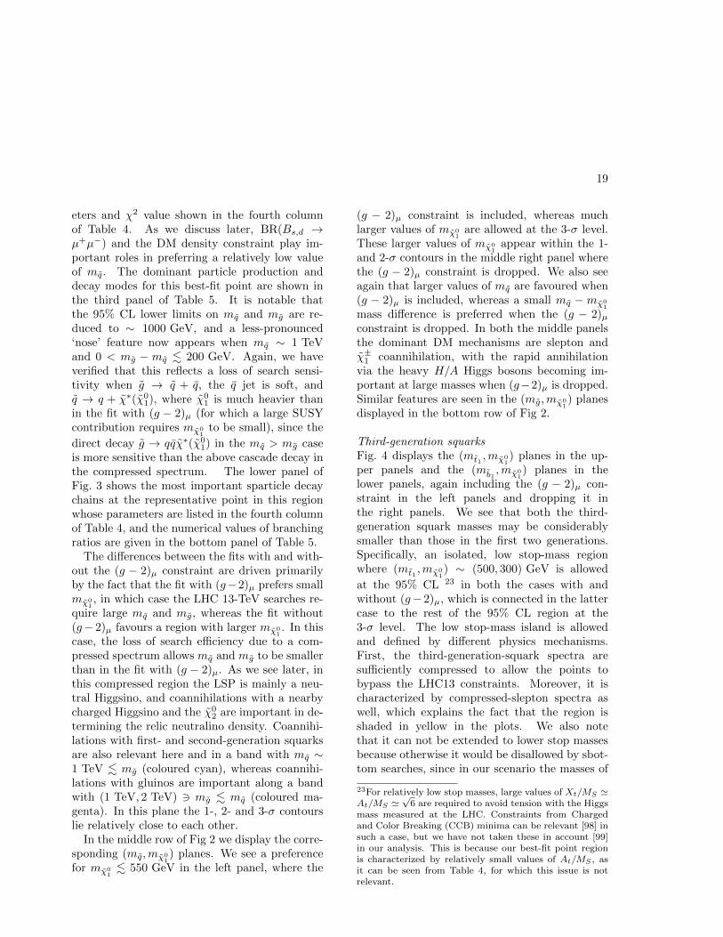
Squarks and gluinosThe top row of plots in Fig. 2 show (mq,mg)planes, where mq is an average over the massesof the left- and right-handed first- and second-generation squarks, which are very similar inthe pMSSM11 22. In the top left panel, where(g−2)µ is included, we see 95% CL lower boundsmq & 2000 GeV and mg & 1400 GeV, withregions favoured at the 68% CL appearing atslightly larger masses. We note that the best-fit point, denoted by the green star, is at largemq > 4000 GeV and mg ∼ 3900 GeV. The fullset of pMSSM parameter values at this point, aswell as the value of the global χ2 function, arelisted in the second column of Table 4. Impor-tant sparticle production cross-sections and decaymodes at this best-fit point are shown in the toppanel of Table 5.

Within the 2-σ contour, the dominant DMmechanism is slepton coannihilation, with staucoannihilation also playing a role for mq ∼2.5 TeV, and χ±1 coannihilation playing a role atmg ∼ 1500 GeV and when mg & 2500 GeV andmq & 2800 GeV. Finally, we observe that at the3-σ level much smaller values of mq are allowed,and that there is also a peninsula at small mg

and larger mq that appears at the same level.

22This and later figures were prepared usingMatplotlib [97], except where otherwise noted.

14

0

400

800

1200

1600

2000

2400

2800

3200

3600

4000

4400

Mas

s/

GeV

h0

H0A0

H±gqRqL

t1

b1

b2t2

˜R

νL

˜Lτ1

ντ

τ2

χ01

χ02 χ±

1

χ03

χ04 χ±

2

0

400

800

1200

1600

2000

2400

2800

3200

Mas

s/

GeV

h0

H0A0

H±

qR

qL

t1

b1b2

t2

˜R

νL

˜L

τ1

ντ

τ2

g

χ01

χ02 χ±

1

χ03

χ04 χ±

2

Figure 1. Higgs and sparticle spectra for the best-fit points for the pMSSM11 with (top) and without the(g−2)µ constraint (bottom), showing also decay paths with branching ratios > 5%, the widths of the linesbeing proportional to the branching ratios. These plots were prepared using the code presented in [96].

15

Parameter With LHC 13 TeV and (g − 2)µ With LHC 13 TeV, not (g − 2)µ

Best fit ‘Nose’ region Best fit ‘Nose’ region

M1 0.25 TeV - 0.39 TeV - 1.3 TeV - 1.5 TeV

M2 0.25 TeV 1.2 TeV 2.3 TeV 2.0 TeV

M3 - 3.86 TeV - 1.7 TeV 1.9 TeV 1.0 TeV

mq 4.0 TeV 2.00 TeV 0.9 TeV 0.9 TeV

mq3 1.7 TeV 4.1 TeV 2.0 TeV 1.9 TeV

m˜ 0.35 TeV 0.36 TeV 1.9 TeV 1.4 TeV

mτ 0.46 TeV 1.4 TeV 1.3 TeV 1.4 TeV

MA 4.0 TeV 4.2 TeV 3.0 TeV 3.3 TeV

A 2.8 TeV 5.4 TeV - 3.4 TeV - 3.4 TeV

µ 1.33 TeV - 5.7 TeV - 0.95 TeV - 0.93 TeV

tanβ 36 19 33 33

χ2/d.o.f. 22.1/20 24.46/20 20.88/19 22.57/19

p-value 0.33 0.22 0.34 0.25

χ2(HS) 68.01 67.97 68.06 68.05

Table 4Values of the pMSSM11 input parameters and values of the global χ2 function at the best-fit pointsincluding the LHC 13-TeV constraints, with and without the (g−2)µ constraint, as well as at representativepoints in the ‘nose’ regions in the top left and right panels of Fig. 2. Lower rows show the total χ2/d.o.f.and the corresponding p-values for each point. As discussed in the text, we calculate these omittingthe contributions from HiggsSignals, which are shown separately in the last line. The SLHA files forthese points are available on our website, at the following URL https: // mastercode. web. cern. ch/

mastercode/ downloads. php .

These regions avoid the LHC exclusion searches invirtue of the same mechanisms which allow lowermasses when the (g−2)µ constraint is not appliedand which will be described more in detail below.However, they are not able to satisfy the (g− 2)µand this is why they take a ∆χ2 ' 11 penaltywhich makes them allowed only at 3-σ.

We also note a ‘nose’ feature correspondingto a reduction in the lower bounds when mq ∼2.2 TeV and 0 < mq − mg . 200 GeV. Wehave verified that this is due to a loss of searchsensitivity when qR → g + q, the q jet is soft,and g → qq + χ∗, where χ∗ denotes any elec-troweak ino other than the LSP, compared to ahigh sensitivity for qR → qχ0

1 in the mg > mq

case. The input pMSSM11 parameter values at

a representative point in this ‘nose’ region arelisted in the third column of Table 4. The upperpanel of Fig. 3 displays relevant sparticle massesand the most important sparticle decay chainsat this point, and numerical values are given inthe second panel of Table 5. We see that theright-handed squarks decay into a variety of finalstates involving heavier neutralinos and charginosvia intermediate gluinos due to mg < mq, reduc-ing the effectiveness of /ET -based searches in this‘nose’ region, compared to simple q → q + χ0

1 de-cays.

We see significant differences in the top rightpanel where (g − 2)µ is dropped. The best-fitin this case is close to the 68% CL boundary at(mq,mg) ∼ (1000, 1600) GeV, with the param-

https://mastercode.web.cern.ch/mastercode/downloads.php

https://mastercode.web.cern.ch/mastercode/downloads.php

16

0 500 1000 1500 2000 2500 3000 3500 4000

mq [GeV]

0

500

1000

1500

2000

2500

3000

3500

4000

mg[GeV

]

pMSSM11 w/ (g − 2)µ : best fit, 1σ, 2σ, 3σ

0 500 1000 1500 2000 2500 3000 3500 4000

mq [GeV]

0

500

1000

1500

2000

2500

3000

3500

4000

mg[GeV

]

pMSSM11 w/o (g − 2)µ : best fit, 1σ, 2σ, 3σ

0 500 1000 1500 2000 2500 3000 3500 4000

mq [GeV]

0

200

400

600

800

1000

1200

mχ

0 1[GeV

]


0 500 1000 1500 2000 2500 3000 3500 4000

mq [GeV]

0

200

400

600

800

1000

1200

mχ

0 1[GeV

]


0 500 1000 1500 2000 2500 3000 3500 4000

mg [GeV]

0

200

400

600

800

1000

1200

mχ

0 1[GeV

]


0 500 1000 1500 2000 2500 3000 3500 4000

mg [GeV]

0

200

400

600

800

1000

1200

mχ

0 1[GeV

]


±1 coann.

A/H funnelslep coann.stau coann.

gluino coann.squark coann.

stop coann.sbot coann.

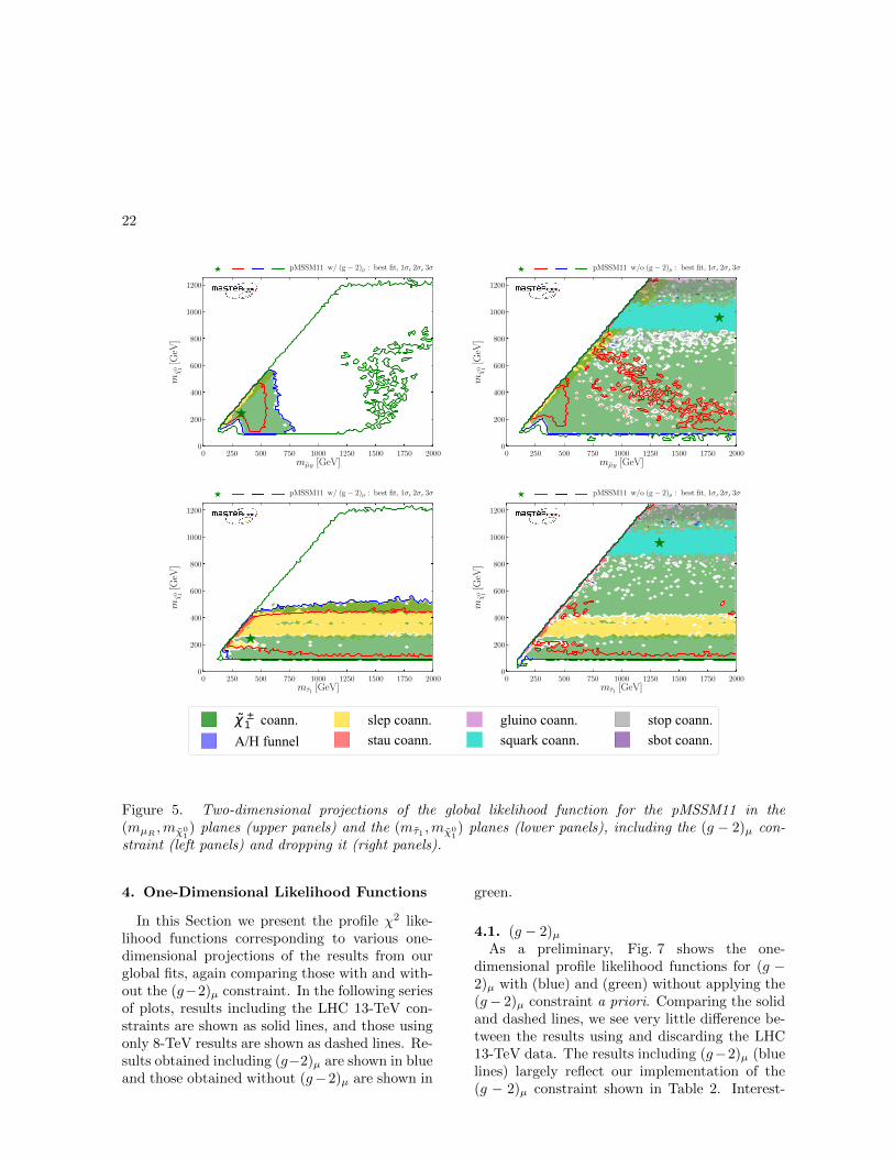
Figure 2. Two-dimensional projections of the global likelihood function for the pMSSM11 in the (mq,mg)planes (top panels), the (mq,mχ0

1) planes (middle panels) and the (mt1

,mχ01) planes (bottom panels),

including the (g − 2)µ constraint (left panels) and dropping it (right panels).

17

29

0

500

1000

1500

2000

Mas

s[G

eV]

uL

±1 +j

g+j

01+j

02+j

eR+l

01+[g, W+, bb, Z, tt, jj, h]

02+[g, tt, jj, bb]

±1 +[bt, jj]

eL+l

e+l

µR+lµ+l

µL+l

eR+l

01+[Z, W+, l, h]

eL+l

e+l

µR+lµ+l

µL+l 01+l

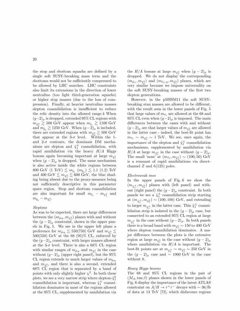
Figure 3. Upper panel: The dominant sparticle decay chains at the representative point in the ‘nose’region in the top left panel of Fig. 2 (with (g 2)µ) whose parameters are listed in the second columnof Table 4. Lower panel: The dominant sparticle decay chains at the representative point in the ‘nose’region in the top right panel of Fig. 2 (without (g 2)µ) whose parameters are listed in the fourth columnof Table 4 - note that the vertical scale has a suppressed zero.

g

χ±1 χ0

2

ℓ, ν χ01

[tb,tb, q

q]

[ℓ, ν]

[ℓ,ν]

[ℓ, ν]

[W ±]

[Z, h

]

29


[qq,

bb, t

t ]

[qq,

bb, t

t ]

qL

[q][q]

[q]

[q] [q]

[q]

qR

29

900

950

1000

1050

1100

Mas

s[G

eV]

g

dR+j uR+j

sL+j

cL+jsR+j

dL+j

cR+j

uL+j

±1 +j

01+j

02+j

±1 +[jj, ll]

01+[, jj, ll] 0

1+[jj, ll]


qL

g

χ±1

χ02

qR

[q] [q]

[q]

[q] [q]

[qq, ℓν]

χ01

[q]

[γ, qq, νν, ℓℓ]

29


Figure 3. Upper panel: The dominant sparticle decay chains at the representative point in the ‘nose’region in the top left panel of Fig. 2 (with (g − 2)µ) whose parameters are listed in the second columnof Table 4. Lower panel: The dominant sparticle decay chains at the representative point in the ‘nose’region in the top right panel of Fig. 2 (without (g− 2)µ) whose parameters are listed in the fourth columnof Table 4 - note that the vertical scale has a suppressed zero. In both plots the widths of the sparticlesare represented as semi-transparent bands around the bar representing the nominal mass value and of thesame color.

18

Dominant sparticle production and decay modes at best-fit point with (g − 2)µ

Production σ [fb]

pp→ t1t1 + X 0.25

pp→ b1b1 + X 0.13

Decays (mass [GeV]) BR [%]

t1(1481) → bχ±1 (270) / tχ02(270) / tχ0

1(249) 56 / 25 / 19

b1(1586) → tχ±1 (270) / bχ02(270) / bχ0

3/4(270) / bχ01(249) 60 / 29 / 5 / 4

χ±1 (270) → `±ν`χ01(249) / qq′χ0

1(249) / τ±ντ χ01(249) 52 / 38 / 1

χ02(270) → ννχ0

1(249) / `±`∓χ01(249) / τ±τ∓χ0

1(249) 53 / 37 / 1

Dominant sparticle production and decay modes at ‘nose’ point in fit with (g − 2)µ

Production σ [fb]

pp→ qq + X 3.4

pp→ gq + X 3.4

pp→ gg + X 0.5


g(1942) → qqχ01(380) / qq′χ±1 (1273) / qqχ0

2(1273) 45 / 37 / 18

qL(2099) → qχ±1 (1273) / qg(1942) / qχ02(1273) / qχ0

1(380) 48 / 26 / 24 / 2

qR(2086) → qg(1942) / qχ01(380) 57 / 43

χ±1 (1273) → [`±ν`(400)→ `±ν`χ01(380)] / [ν` ˜

±(404)→ ν``±χ0

1(380)] 50 / 50

χ02(1273) → [`± ˜∓(404)→ `+`−χ0

1(380)] / [νν`(400)→ ν`ν`χ01(380)] 50 / 50

Dominant sparticle production and decay modes at best-fit point without (g − 2)µ

Production σ [fb]

pp→ qq + X 386

pp→ gq + X 51

pp→ gg + X 1


g(1908) → qqR(988) / qqL(1008) 51 / 49

qL(1008) → qχ±1 (955) / qχ01(954) / qχ0

2(954) 55 / 39 / 6

qR(988) → qχ02(954) / qχ0

1(954) 98 / 2

Dominant sparticle production and decay modes at ‘nose’ point in fit without (g − 2)µ

Production σ [fb]

pp→ qq + X 619

pp→ gq + X 586

pp→ gg + X 87


g(1131) → qqR(984) / qqL(1003) 44 / 56

qL(1003) → qχ±1 (939) / qχ01(937) / qχ0

2(938) 58 / 38 / 4

qR(984) → qχ02(938) / qχ0

1(937) 96 / 4Table 5Dominant particle production and decay modes for various pMSSM11 parameter sets. Top panel: best-fitpoint with (g − 2)µ. Second panel: representative point in the ‘nose’ region in fit with (g − 2)µ. Thirdpanel: best-fit point without (g−2)µ. Bottom panel: representative point in the ‘nose’ region in fit without(g − 2)µ.

19

eters and χ2 value shown in the fourth columnof Table 4. As we discuss later, BR(Bs,d →µ+µ−) and the DM density constraint play im-portant roles in preferring a relatively low valueof mq. The dominant particle production anddecay modes for this best-fit point are shown inthe third panel of Table 5. It is notable thatthe 95% CL lower limits on mq and mg are re-duced to ∼ 1000 GeV, and a less-pronounced‘nose’ feature now appears when mq ∼ 1 TeVand 0 < mg − mq . 200 GeV. Again, we haveverified that this reflects a loss of search sensi-tivity when g → q + q, the q jet is soft, andq → q + χ∗(χ0

1), where χ01 is much heavier than

in the fit with (g − 2)µ (for which a large SUSYcontribution requires mχ0

1to be small), since the

direct decay g → qqχ∗(χ01) in the mq > mg case

is more sensitive than the above cascade decay inthe compressed spectrum. The lower panel ofFig. 3 shows the most important sparticle decaychains at the representative point in this regionwhose parameters are listed in the fourth columnof Table 4, and the numerical values of branchingratios are given in the bottom panel of Table 5.

The differences between the fits with and with-out the (g − 2)µ constraint are driven primarilyby the fact that the fit with (g−2)µ prefers smallmχ0

1, in which case the LHC 13-TeV searches re-

quire large mq and mg, whereas the fit without(g− 2)µ favours a region with larger mχ0

1. In this

case, the loss of search efficiency due to a com-pressed spectrum allows mq and mg to be smallerthan in the fit with (g − 2)µ. As we see later, inthis compressed region the LSP is mainly a neu-tral Higgsino, and coannihilations with a nearbycharged Higgsino and the χ0

2 are important in de-termining the relic neutralino density. Coannihi-lations with first- and second-generation squarksare also relevant here and in a band with mq ∼1 TeV . mg (coloured cyan), whereas coannihi-lations with gluinos are important along a bandwith (1 TeV, 2 TeV) 3 mg . mq (coloured ma-genta). In this plane the 1-, 2- and 3-σ contourslie relatively close to each other.

In the middle row of Fig 2 we display the corre-sponding (mq,mχ0

1) planes. We see a preference

for mχ01. 550 GeV in the left panel, where the

(g − 2)µ constraint is included, whereas muchlarger values of mχ0

1are allowed at the 3-σ level.

These larger values of mχ01

appear within the 1-and 2-σ contours in the middle right panel wherethe (g − 2)µ constraint is dropped. We also seeagain that larger values of mq are favoured when(g − 2)µ is included, whereas a small mq − mχ0

1

mass difference is preferred when the (g − 2)µconstraint is dropped. In both the middle panelsthe dominant DM mechanisms are slepton andχ±1 coannihilation, with the rapid annihilationvia the heavy H/A Higgs bosons becoming im-portant at large masses when (g−2)µ is dropped.Similar features are seen in the (mg,mχ0

1) planes

displayed in the bottom row of Fig 2.

Third-generation squarksFig. 4 displays the (mt1

,mχ01) planes in the up-

per panels and the (mb1,mχ0

1) planes in the

lower panels, again including the (g − 2)µ con-straint in the left panels and dropping it inthe right panels. We see that both the third-generation squark masses may be considerablysmaller than those in the first two generations.Specifically, an isolated, low stop-mass regionwhere (mt1

,mχ01) ∼ (500, 300) GeV is allowed

at the 95% CL 23 in both the cases with andwithout (g− 2)µ, which is connected in the lattercase to the rest of the 95% CL region at the3-σ level. The low stop-mass island is allowedand defined by different physics mechanisms.First, the third-generation-squark spectra aresufficiently compressed to allow the points tobypass the LHC13 constraints. Moreover, it ischaracterized by compressed-slepton spectra aswell, which explains the fact that the region isshaded in yellow in the plots. We also notethat it can not be extended to lower stop massesbecause otherwise it would be disallowed by sbot-tom searches, since in our scenario the masses of

23For relatively low stop masses, large values of Xt/MS 'At/MS '

√6 are required to avoid tension with the Higgs

mass measured at the LHC. Constraints from Chargedand Color Breaking (CCB) minima can be relevant [98] insuch a case, but we have not taken these in account [99]in our analysis. This is because our best-fit point regionis characterized by relatively small values of At/MS , asit can be seen from Table 4, for which this issue is notrelevant.

20

the stop and sbottom squarks are defined by asingle soft SUSY-breaking mass term and thesbottoms would not be sufficiently compressed tobe allowed by LHC searches. LHC constraintsalso limit its extensions in the direction of lowerneutralino (too light third-generation squarks)or higher stop masses (due to the loss of com-pression). Finally, at heavier neutralino massesslepton coannihilation is insufficient to reducethe relic density into the allowed range.4 When(g−2)µ is dropped, extended 95% CL regions withmχ0

1& 500 GeV appear when mt1

& 1100 GeVand mb1

& 1250 GeV. When (g−2)µ is included,there are extended regions with mχ0

1& 500 GeV

that appear at the 3-σ level. Within the 1-and 2-σ contours, the dominant DM mecha-nisms are slepton and χ±1 coannihilation, withrapid annihilation via the heavy H/A Higgsbosons again becoming important at large mχ0

1

when (g − 2)µ is dropped. The same mechanismis also active inside the white regions between800 GeV (1 TeV) . mt1

(mb1) . 1.1 (1.2) TeV

and 400 GeV . mχ01. 600 GeV, the blue shad-

ing being absent due to the proxy-measure beingnot sufficiently descriptive in this parameterspace region. Stop and sbottom coannihilationare also important for small mt1

− mχ01

andmb1−mχ0

1.

SleptonsAs was to be expected, there are large differencesbetween the (mµR

,mχ01) planes with and without

the (g − 2)µ constraint, shown in the upper pan-els in Fig. 5. We see in the upper left plane apreference for mµR

. 550(750) GeV and mχ01.

500(550) GeV at the 68 (95)% CL, enforced bythe (g−2)µ constraint, with larger masses allowedat the 3-σ level. There is also a 68% CL regionwith similar ranges of mµR

and mχ01

in the casewithout (g−2)µ (upper right panel), but the 95%CL region extends to much larger values of mµR

and mχ01, and there is also a second, extended

68% CL region that is separated by a band ofpoints with only slightly higher χ2. In both theseplots, we see a very narrow strip where slepton-χ0

1

coannihilation is important, whereas χ±1 coanni-hilation dominates in most of the regions allowedat the 95% CL, supplemented by annihilation via

the H/A bosons at large mχ01

when (g − 2)µ isdropped. We do not display the corresponding(mµL

,mχ01) and (meL,R

,mχ01) planes, which are

very similar because we impose universality onthe soft SUSY-breaking masses of the first twoslepton generations.

However, in the pMSSM11 the soft SUSY-breaking stau masses are allowed to be different,with the result seen in the lower panels of Fig. 5that large values of mτ1 are allowed at the 68 and95% CL even when (g−2)µ is imposed. The maindifferences between the cases with and without(g− 2)µ are that larger values of mχ0

1are allowed

in the latter case - indeed, the best-fit point hasmτ1 ∼ mχ0

1∼ 1 TeV. We see, once again, the

importance of the slepton and χ±1 coannihilationmechanisms, supplemented by annihilation viaH/A at large mχ0

1in the case without (g − 2)µ.

The small ‘nose’ at (mτ1 ,mχ01) ∼ (100, 50) GeV

is a remnant of rapid annihilations via direct-channel Z and h(125) poles.

Electroweak inosIn the upper panels of Fig. 6 we show the(mχ±

1,mχ0

1) planes with (left panel) and with-

out (right panel) the (g− 2)µ constraint. In bothpanels we see a χ±1 coannihilation strip startingat (mχ±

1,mχ0

1) ∼ (100, 100) GeV, and extending

to larger mχ±1

in the latter case. This χ±1 coanni-

hilation strip is isolated in the (g − 2)µ case, butconnected to an extended 95% CL region at largemχ±

1in the case without (g− 2)µ. In both panels

there is a broad band with mχ01∼ 150 to 400 GeV

where slepton coannihilation dominates. A ma-jor difference between the plots is the extensiveregion at large mχ0

1in the case without (g − 2)µ

where annihilation via H/A is important. Thebest-fit points are at mχ±

1∼ mχ0

1∼ 250 GeV in

the (g − 2)µ case and ∼ 1000 GeV in the casewithout it.

Heavy Higgs bosonsThe 68 and 95% CL regions in the pair of(MA, tanβ) planes shown in the lower panels ofFig. 6 display the importance of the latest ATLASconstraint on A/H → τ+τ− decays with ∼ 36/fbof data at 13 TeV [72], which disfavours regions

21

0 250 500 750 1000 1250 1500 1750 2000mt1

[GeV]0

200

400

600

800

1000

1200

mχ

0 1[GeV

]


0 250 500 750 1000 1250 1500 1750 2000mt1

[GeV]0

200

400

600

800

1000

1200

mχ

0 1[GeV

]


0 250 500 750 1000 1250 1500 1750 2000mb1

[GeV]0

200

400

600

800

1000

1200

mχ

0 1[GeV

]


0 250 500 750 1000 1250 1500 1750 2000mb1

[GeV]0

200

400

600

800

1000

1200

mχ

0 1[GeV

]


±1 coann.




Figure 4. Two-dimensional projections of the global likelihood function for the pMSSM11 in the (mt1,mχ0

1)

planes (upper panels) and the (mb1,mχ0

1) planes (lower panels), including the (g − 2)µ constraint (left

panels) and dropping it (right panels).

with MA . 1 TeV at larger tanβ. We also notethat the dominant DM mechanisms display signif-icant differences. Chargino coannihilation is im-portant in both planes, but slepton coannihilationappears only in the case where (g−2)µ is included.In this case annihilation via the H/A poles ap-pears only when MA . 1 TeV, but it appears alsoat larger MA when (g − 2)µ is dropped. We seein both cases a limited region with MA ∼ 2 TeVand tanβ . 10 where stau coannihilation dom-inates. In our previous pMSSM10 analysis [10]the interplay of the LHC electroweak searches,

(g − 2)µ and the DM constraints, heavily rely-ing on the fact that only one independent sleptonmass parameter was allowed, led to a region with25 <∼ tanβ <∼ 45 being preferred at the 68% CL.However, in the pMSSM11, dropping the restric-tion mτ = m˜ now allows values of tanβ < 5 fora wide range of MA values. Also, despite the up-dated (stronger) constraints on H/A → ττ , val-ues down to MA ∼ 500 GeV are still allowed atthe 95% CL.

22

0 250 500 750 1000 1250 1500 1750 2000mµR

[GeV]

0

200

400

600

800

1000

1200

mχ

0 1[GeV

]


0 250 500 750 1000 1250 1500 1750 2000mµR

[GeV]

0

200

400

600

800

1000

1200

mχ

0 1[GeV

]


0 250 500 750 1000 1250 1500 1750 2000mτ1

[GeV]

0

200

400

600

800

1000

1200

mχ

0 1[GeV

]


0 250 500 750 1000 1250 1500 1750 2000mτ1

[GeV]

0

200

400

600

800

1000

1200

mχ

0 1[GeV

]


±1 coann.




Figure 5. Two-dimensional projections of the global likelihood function for the pMSSM11 in the(mµR

,mχ01) planes (upper panels) and the (mτ1 ,mχ0

1) planes (lower panels), including the (g − 2)µ con-

straint (left panels) and dropping it (right panels).

4. One-Dimensional Likelihood Functions

In this Section we present the profile χ2 like-lihood functions corresponding to various one-dimensional projections of the results from ourglobal fits, again comparing those with and with-out the (g−2)µ constraint. In the following seriesof plots, results including the LHC 13-TeV con-straints are shown as solid lines, and those usingonly 8-TeV results are shown as dashed lines. Re-sults obtained including (g−2)µ are shown in blueand those obtained without (g−2)µ are shown in

green.

4.1. (g − 2)µAs a preliminary, Fig. 7 shows the one-

dimensional profile likelihood functions for (g −2)µ with (blue) and (green) without applying the(g− 2)µ constraint a priori. Comparing the solidand dashed lines, we see very little difference be-tween the results using and discarding the LHC13-TeV data. The results including (g−2)µ (bluelines) largely reflect our implementation of the(g − 2)µ constraint shown in Table 2. Interest-

23

0 250 500 750 1000 1250 1500 1750 2000mχ±

1[GeV]

0

200

400

600

800

1000

1200

mχ

0 1[GeV

]


0 250 500 750 1000 1250 1500 1750 2000mχ±

1[GeV]

0

200

400

600

800

1000

1200

mχ

0 1[GeV

]


0 1000 2000 3000 4000

MA[GeV]0

10

20

30

40

50

60

tanβ


0 1000 2000 3000 4000

MA[GeV]0

10

20

30

40

50

60

tanβ


±1 coann.




Figure 6. Two-dimensional projections of the global likelihood function for the pMSSM11 in the(mχ±

1,mχ0

1) planes (upper panels) and the (MA, tanβ) planes (lower panels), including the (g − 2)µ

constraint (left panels) and dropping it (right panels).

ingly, when this constraint is not applied a priori(green lines), whilst a very small SUSY contri-bution to (g − 2)µ is preferred, a wide range ofvalues of (g − 2)µ are found to be allowed at the∆χ2∼ 2 level and the experimental value can beaccommodated at the 1.5-σ level. Although theother data certainly do not favour a large SUSYcontribution to (g − 2)µ, neither do they excludeit.

4.2. Sparticle Masses

Squarks and gluinosThe profile likelihood functions for squarks andgluinos are shown in Fig. 8. The left panel isfor mq, where we see that when the 13-TeVLHC data and (g − 2)µ constraint are included(solid blue line), there is a monotonic decreasein χ2 as mq increases, with mq & 1.9 TeV atthe 95% CL (horizontal dotted line). This con-straint is much stronger than that obtained with8-TeV data alone (dashed blue and green lines):

24

−1 0 1 2 3 4 5 6

∆(g−22

)µ

×10−9

0

2

4

6

8∆χ2

pMSSM11LHC13, w/ (g − 2)µ

LHC8, w/ (g − 2)µ

LHC13, w/o (g − 2)µ

LHC8, w/o (g − 2)µ

Figure 7. One-dimensional profile likelihood functions for (g − 2)µ in the pMSSM11, with (blue) andwithout (green) applying the (g − 2)µ constraint a priori and with (solid) and without (dashed) applyingthe constraints coming from the LHC run at 13 TeV. Also shown as a dotted line is the experimentalconstraint [54], taking into account the theoretical uncertainty [53] within the Standard Model.

mq & 1.0 TeV at the 95% CL. In particular,the 13-TeV data exclude a squark coannihilationstrip that had been allowed by the 8-TeV data.When (g−2)µ is dropped but the 13-TeV data re-tained (solid green line), the χ2 function exhibitsa global minimum at mq ∼ 1 TeV, with a plateauat ∆χ2 ' 1.5 at larger mq. Important roles inthe location of this global minimum are played bythe BR(Bs,d → µ+µ−) constraint as discussed inSubsection 4.4, whose contribution to the globalχ2 function at this point is ∼ 1.1 lower than atlarge mq, and by the relic DM density constraint,which is satisfied thanks to multiple coannihila-tion processes as discussed in Subsection 4.6.

In the right panel of Fig. 8 for mg, we see thatwith both the LHC 13-TeV data and (g − 2)µincluded mg & 1.8 TeV (solid blue line), whereaswithout (g − 2)µ we find mg & 1.0 TeV (solidgreen line). On the other hand, in the ab-sence of the LHC 13-TeV data (dashed lines),mg & 500 GeV would have been allowed at the95% CL, whether (g − 2)µ is included, or not.

The LHC 13-TeV run has excluded a region ofgluino coannihilation that was allowed by the8-TeV data.

Third-generation squarksAn analogous pair of plots showing the profilelikelihood functions for the masses of the t1 andb1 are shown in the left and right panels of Fig. 9.When the LHC 13-TeV data are included we seein the left panel a well-defined local minimum ofthe χ2 function in a compressed-stop region with∆χ2 ∼ 2.3 for mt1

∼ 400 GeV. This is followedby a local maximum that exceeds ∆χ2 > 9 formt1∼ 800 GeV when (g − 2)µ is included (solid

blue line) but is lower when (g − 2)µ is dropped(solid green line). This is followed in both casesby a monotonic decrease for larger mt1

and aglobal minimum of χ2 for mt1

∼ 1800 GeV.In the case of mb1

(right panel of Fig. 9). whenthe 13-TeV LHC data and (g − 2)µ are included(solid blue line) there are some irregularities inthe χ2 function for mb1

∼ 1000 GeV, but no hint

25

0 1000 2000 3000 4000mq [GeV]

0

2

4

6

8

∆χ2


LHC8, w/ (g − 2)µ

LHC13, w/o (g − 2)µ

LHC8, w/o (g − 2)µ

0 1000 2000 3000 4000mg [GeV]

0

2

4

6

8

∆χ2


LHC8, w/ (g − 2)µ

LHC13, w/o (g − 2)µ

LHC8, w/o (g − 2)µ

Figure 8. Left panel: one-dimensional profile likelihood functions for the q mass in the pMSSM11 with(blue) and without the (g − 2)µ constraint (green) and with (solid) and without (dashed) applying theconstraints from LHC Run II. Right panel: similarly for the g mass.

of a compressed-sbottom region when (g − 2)µis dropped (dashed blue line). Comparing withthe situation when only LHC 8-TeV used, we seethat the 13-TeV data have increased significantlythe pressure on scenarios with mb1

. 1.5 TeV.

At larger masses the χ2 functions mb1are very

similar to those for mt1, whether (g − 2)µ is in-

cluded or not.

SleptonsFig. 10 displays analogous plots of the profile like-lihood functions for mµR

(left panel, those formµL

and meL,Rare very similar) and mτ1 (right

panel, that for mτ2 is quite similar). When the(g − 2)µ constraint is implemented (blue lines),the χ2 function for mµR

exhibits the expectedwell-defined minimum at mµR

∼ 200 to 500 GeVwhen the LHC 13-TeV data are included. In theabsence of the (g − 2)µ constraint (green lines),this is replaced by a plateau with ∆χ2 ∼ 2 thatextends to mµR

∼ 900 GeV, where the profilelikelihood function drops to very small values forlarger mµR

. The drop occurs because this fitprefers mχ0

1∼ 900 to 1000 GeV, and any heavier

µR can decay into a χ01 in this mass range.

We see in the right panel of Fig. 10 that when

(g − 2)µ is included (blue lines) the profile likeli-hood function for mτ1 is quite different from thatfor mµR

, thanks to the decoupling between theirsoft SUSY-breaking masses in the pMSSM11.The χ2 function falls monotonically to a localminimum when mτ1 ∼ 300 GeV and remainssmall for larger mτ1 , whether the LHC 13-TeVdata are included (solid line), or not (dashedline). However, when (g − 2)µ is dropped (greenlines), the profile likelihood function for mτ1 isquite similar to that for mµR

, also exhibiting aplateau with ∆χ2 ∼ 2 and falling to small valuesfor mτ1 & 900 GeV when the LHC 13-TeV dataare included. This feature appears because, inorder to avoid a charged LSP, a smaller value ofmτ1 would require a smaller value of mχ0

1, which

is disfavoured as seen in the left panel of Fig. 11and discussed below.

Electroweak inosFig. 11 shows the profile likelihood functions forthe lightest neutralino χ0

1 (left panel) and thelighter chargino χ±1 (right panel). When the(g − 2)µ constraint is applied (blue lines), the χ2

function for mχ01

including 13-TeV data exhibitsa well-defined but broad minimum at mχ0

1∼ 100

26

0 1000 2000 3000 4000mt1

[GeV]

0

2

4

6

8

∆χ2


LHC8, w/ (g − 2)µ

LHC13, w/o (g − 2)µ

LHC8, w/o (g − 2)µ

0 1000 2000 3000 4000mb1

[GeV]

0

2

4

6

8

∆χ2


LHC8, w/ (g − 2)µ

LHC13, w/o (g − 2)µ

LHC8, w/o (g − 2)µ

Figure 9. Left panel: one-dimensional profile likelihood functions for the t1 mass in the pMSSM11 with(blue) and without the (g − 2)µ constraint (green) and with (solid) and without (dashed) applying the

constraints from LHC Run II. Right panel: similarly for the b1 mass.

to 400 GeV. This preference for small mχ01

wasalready seen in the upper boundaries of the 68%and 95% CL regions in the planes involving mχ0

1

shown in the previous Section when the (g − 2)µconstraint is applied (left panels).

On the other hand, when the (g−2)µ constraintis dropped (green lines) we see a preference formχ0

1∼ 950 GeV. Despite the fact that the LSP

is a nearly-pure Higgsino at this best-fit point,this mass of ∼ 950 GeV is below the ∼ 1.1 TeVmass expected for a Higgsino dark matter candi-date. This arises because, at the best-fit point,several of the squark masses lie close to the LSPmass, making multiple coannihilation important.Due to the relatively large number of states withmasses close to the Higgsino, their density ac-tually increases the final LSP relic density 24,thereby pushing the mass of the Higgsino belowits nominal ∼ 1.1 TeV value.

Turning now to the profile likelihood func-tions for the lighter chargino χ±1 (right panelof Fig. 11), we see that when (g − 2)µ is takeninto account (blue lines) the χ2 function alsofeatures a well-defined minimum for mχ±

1∼ 200

24This effect was noted previously in a different contextin [100].

to 500 GeV (that for χ02 is very similar), reflect-

ing the importance of χ±1 − χ01 coannihilation.

This minimum is followed by a rise to a localmaximum at mχ±

1∼ 600 GeV, which is more

pronounced when the 13-TeV data are included(solid blue), followed by a slow decrease as mχ±

1

increases further. When the (g−2)µ constraint isdropped and the LHC 13-TeV data are included(solid green line), the χ2 functions for mχ±

1and

mχ02

have global minima at mχ01∼ 1000 GeV, ac-

companied by plateaus with ∆χ2 ∼ 2 at smallerand larger values of mχ±

1. The dip in the χ2 func-

tion occurs because the fit to BR(Bs,d → µ+µ−)is improved for mχ±

1' mχ0

2∼ mχ0

1∼ 1 TeV.

Chargino coannihilation is important around thisglobal minimum of the χ2 function, and so areother coannihilation mechanisms, as we discusslater.

4.3. Neutralino CompositionIt is interesting also to examine the profile like-

lihood functions for the amplitudes N1i charac-terizing the χ0

1 composition:

χ01 = N11B +N12W

3 +N13Hu +N14Hd , (18)

27

0 500 1000 1500 2000mµR

[GeV]

0

2

4

6

8

∆χ2


LHC8, w/ (g − 2)µ

LHC13, w/o (g − 2)µ

LHC8, w/o (g − 2)µ

0 500 1000 1500 2000mτ1

[GeV]

0

2

4

6

8

∆χ2


LHC8, w/ (g − 2)µ

LHC13, w/o (g − 2)µ

LHC8, w/o (g − 2)µ

Figure 10. Left panel: one-dimensional profile likelihood functions for the µR mass in the pMSSM11 with(blue) and without the (g − 2)µ constraint (green) and with (solid) and without (dashed) applying theconstraints from LHC Run II. Right panel: similarly for the τ1 mass.

which are shown in Fig. 12, again for the analysiswith the 13-TeV data as solid lines and withoutthem as dashed lines, and with (g − 2)µ as bluelines and without it as green lines. The top leftpanel shows that, when (g − 2)µ is included, an

almost pure B composition of the χ01 is preferred,

N11 → 1, though the possibility that this compo-nent is almost absent is also allowed at the level∆χ2 ∼ 4. On the other hand, when the con-straint from (g − 2)µ is removed, there is a mild(∆χ2 ∼ 1) preference for N11 → 0. The reasonfor this is again the preference for a large Hu,d

components in the latter case, where the neu-tralino mass is allowed to be larger, due to flavorconstraints slightly favoring a 1 TeV neutralino asa solution to the observed DM relic density. Theupper right panel shows that a small W 3 compo-nent in the χ0

1 is preferred in all cases. 25. Finally,the lower panel confirms that small Hu,d compo-nents are preferred by ∆χ2 & 4 when (g − 2)µ isincluded, whereas there would have been a pref-erence for these components to dominate in theabsence of the (g − 2)µ constraint.

25This is because we only scan m˜ and mτ < 2 TeV, hencemχ0

1< 2 TeV, so do not probe the expected Wino-like

LSP region where mχ01∼ 3 TeV.

Fig. 13 displays information about the pre-ferred and disfavoured χ0

1 compositions in two tri-angular panels. Both are for fits including LHC13-TeV data (those dropping these data are quitesimilar), the left panel includes the (g − 2)µ con-straint and the right panel drops it. The ∆χ2 forthe best-fit points at each location in the trianglesare colour-coded as indicated. We see in the leftpanel that in the case with (g−2)µ a small Winofraction N2

12 < 0.1 is strongly favoured, while therelative proportions of the Bino fraction N2

11 andthe Higgsino fraction N2

13 +N214 are relatively un-

constrained at the 95% CL. On the other hand,the right panel shows that almost all binary com-binations of Bino, Wino and Higgsino (along theedges of the triangle) are allowed at the 95% CL,but three-way mixtures (in the interior of the tri-angle) are strongly disfavoured.

Table 6 compares the composition of the LSPχ0

1 found at the best-fit points in our presentpMSSM11 analysis based on LHC 13-TeV data(with and without the (g − 2)µ constraint) withthe composition at the best-fit point from ourprevious pMSSM10 analysis that also applied the(g − 2)µ constraint [10]. We see that both thepMSSM11 and pMSSM10 analyses with (g − 2)µ

28

0 500 1000 1500 2000

mχ0

1[GeV]

0

2

4

6

8

∆χ2


LHC8, w/ (g − 2)µ

LHC13, w/o (g − 2)µ

LHC8, w/o (g − 2)µ

0 500 1000 1500 2000mχ±

1[GeV]

0

2

4

6

8

∆χ2


LHC8, w/ (g − 2)µ

LHC13, w/o (g − 2)µ

LHC8, w/o (g − 2)µ

Figure 11. Left panel: one-dimensional profile likelihood functions for the χ01 mass in the pMSSM11 with

(blue) and without the (g − 2)µ constraint (green) and with (solid) and without (dashed) applying theconstraints from LHC Run II. Right panel: similarly for the χ±1 mass.

prefer an almost pure B composition. On theother hand, when the (g − 2)µ constraint isdropped the pMSSM11 analysis prefers an almostequal mixture of Hu and Hd components witha small admixture of B and again a very smalladmixture of W3 because we only scan m˜ andmτ , hence mχ0

1< 2 TeV. Table 6 also displays

the composition of the second-lightest neutralino,χ0

2, and we see that its content is mainly W3 inthe fit to the pMSSM11 with (g − 2)µ and in thepMSSM10 fit, but is mainly Higgsino in the fit tothe pMSSM11 without (g − 2)µ.

4.4. B-Physics ObservablesFig. 14 displays the one-dimensional profile

likelihood functions for BR(Bs,d → µ+µ−) in thepMSSM11 (left panel) and the BR(Bs → Xsγ)branching ratio (right panel), with and withoutthe LHC 13-TeV data and the (g−2)µ constraint.We see in the left panel that a value of BR(Bs,d →µ+µ−) close to the SM value is preferred if boththese constraints are applied, though deviationsat the level of ± ∼ 10% are allowed at the level of∆χ2 = 4 (2σ), corresponding to the 95% CL. Onthe other hand, if (g − 2)µ is dropped, a larger

range of BR(Bs,d → µ+µ−) is allowed, with alarger deviation at the level of ± ∼ 30% becom-ing allowed at the level of ∆χ2 = 4. In particular,when the LHC13 data are included but (g − 2)µis dropped, the global χ2 function is minimizedat a value of BR(Bs,d → µ+µ−) below the SMvalue, as hinted by the present experimental data,with the SM value being mildly disfavoured by∆χ2 ' 1. It will be interesting to see how mea-surements of BR(Bs,d → µ+µ−) evolve.

The analogous curves for BR(Bs → Xsγ) in theright panel of Fig. 14 show preferences for valuesclose the SM predictions, with 2σ ranges that are±20%. Discriminating between the SM and thepMSSM11 would require significant reductions inboth the theoretical and experimental uncertain-ties in BR(Bs → Xsγ).

As already mentioned in Section 2.3, the LHCbCollaboration has recently announced the firstexperimental measurement of τ(Bs → µ+µ−),which is related to the quantity A∆Γ that takesthe value +1 in the SM, but may be different ina SUSY model such as the pMSSM11. Fig. 15displays the profile likelihood functions for A∆Γ

(left panel) and τ(Bs → µ+µ−)/τBs(right panel),

29

0.0 0.2 0.4 0.6 0.8 1.0N 2

11

0

2

4

6

8

∆χ2


LHC8, w/ (g − 2)µ

LHC13, w/o (g − 2)µ

LHC8, w/o (g − 2)µ

0.0 0.2 0.4 0.6 0.8 1.0N 2

12

0

2

4

6

8

∆χ2


LHC8, w/ (g − 2)µ

LHC13, w/o (g − 2)µ

LHC8, w/o (g − 2)µ

0.0 0.2 0.4 0.6 0.8 1.0N 2

13 +N 214

0

2

4

6

8

∆χ2


LHC8, w/ (g − 2)µ

LHC13, w/o (g − 2)µ

LHC8, w/o (g − 2)µ

Figure 12. One-dimensional likelihood plots for the B fraction in the LSP χ01 composition in the (upper

left), for the W 3 fraction (upper right) and for the Hu,d fraction (lower panel).

30

0.0

1.0

1.0

0.0

0.0 1.00.0

0.1

0.2

0.3

0.4

0.5

0.6

0.7

0.8

0.9

1.0

1.0

0.9

0.8

0.7

0.6

0.5

0.4

0.3

0.2

0.1

0.0

0.0 0.1 0.2 0.3 0.4 0.5 0.6 0.7 0.8 0.9 1.0

Pure higgsino

Pure

bino

Purew

ino

N213 +

N214

N 212

N2

11

pMSSM11 w/ (g − 2)µ χ01 composition

0

2

4

6

8

10

∆χ2

0.0

1.0

1.0

0.0

0.0 1.00.0

0.1

0.2

0.3

0.4

0.5

0.6

0.7

0.8

0.9

1.0

1.0

0.9

0.8

0.7

0.6

0.5

0.4

0.3

0.2

0.1

0.0

0.0 0.1 0.2 0.3 0.4 0.5 0.6 0.7 0.8 0.9 1.0

Pure higgsino

Pure

bino

Purew

inoN 212

N2

11

N213 +

N214

pMSSM11 w/o (g − 2)µ χ01 composition

0

2

4

6

8

10

∆χ2

Figure 13. Triangular presentations of the composition of the χ01 in the fit with LHC 13-TeV and with

(without) the (g − 2)µ constraint in the left (right) panel.

Model State B W3 Hu Hd

pMSSM11 (with (g − 2)µ) χ01 0.99 -0.03 0.04 -0.01

χ02 0.03 0.99 -0.06 -0.01

pMSSM11 (w/o (g − 2)µ) χ01 0.01 0.04 0.71 0.70

χ02 0.09 0.02 -0.70 -0.70

pMSSM10 χ01 0.99 -0.11 0.09 -0.04

χ02 0.12 0.98 -0.13 0.05

Table 6The amplitudes characterizing the decomposition of the LSP χ0

1 and of the χ02 into interaction eigenstates

at the best-fit points in our present pMSSM11 analysis including LHC 13-TeV data, with and without the(g − 2)µconstraint, compared with the composition at the best-fit point found in our previous pMSSM10analysis that also included the (g − 2)µ constraint, but only LHC 8-TeV data [10].

in our pMSSM11 fits with and without the LHC13-TeV data and (g− 2)µ. We restrict our atten-tion to positive values of A∆Γ, corresponding toτ(Bs → µ+µ−)/τBs > 0.94. We see that all thefits favour values of A∆Γ close to unity, with thatdropping both the LHC 13-TeV data and (g−2)µallowing the widest range. Values of τ(Bs →µ+µ−)/τBs

close to unity are also favoured, with∆χ2 & 9 for τ(Bs → µ+µ−)/τBs

= 0.94. The

new LHCb measurement [57] does not challengeany of these model predictions.

4.5. Higgs ObservablesFig. 16 shows similar plots of Mh (upper left

panel), and of the ratios of the branching ratiosfor h→ γγ, ZZ∗ and h→ gg (treated as a proxyfor σ(gg → h)) to their values in the SM in theupper right, lower left and lower right panels, re-spectively. Taking into account the theoretical

31

0.0 0.5 1.0 1.5 2.0

BRMSSM/SMBs,d→µ+µ−

0

2

4

6

8

∆χ2


LHC8, w/ (g − 2)µ

LHC13, w/o (g − 2)µ

LHC8, w/o (g − 2)µ

0.0 0.5 1.0 1.5 2.0

BRMSSM/SMBs→Xsγ

0

2

4

6

8

∆χ2


LHC8, w/ (g − 2)µ

LHC13, w/o (g − 2)µ

LHC8, w/o (g − 2)µ

Figure 14. One-dimensional profile likelihood functions for BR(Bs,d → µ+µ−) in the pMSSM11 (leftpanel) and the BR(Bs → Xsγ) branching ratio (right panel), with and without the LHC 13-TeV dataand the (g − 2)µ constraint. Also shown as dotted lines are the experimental constraints, including thecorresponding theoretical uncertainties within the Standard Model.

uncertainties in the calculation of Mh in a su-persymmetric model [35], which we take to be±3 GeV26, there is no tension with the global fits.These also favour values of the decay branchingratios that are similar to those in the SM whether(g−2)µ is included in the fit, or not, though withuncertainties that are typically ± ∼ 20%. As dis-cussed in [19], the global combination of ATLASand CMS measurements using LHC Run-1 datahas significantly larger uncertainties.

4.6. Dark Matter MeasuresIn Section 2.4 we introduced various possible

mechanisms for bringing the relic χ01 density into

the range allowed by Planck and other data,proposing measures of their prospective impor-tance that we portrayed using different coloursin the two-dimensional parameter planes shownin Section 3. We emphasized there and in thesubsequent discussions of one-dimensional profilelikelihood functions earlier in Section 4 the rolesplayed by certain of these DM mechanisms. In

26We implement the constraint in the fit as a Gaussianlikelihood-penalty with σ = 1.5 GeV, to avoid issues whichwould result from using a flat interval (due to the discon-tinuity in the p.d.f. at the interval extrema).

this Subsection we display profile likelihood func-tions for the most interesting of these DM mea-sures, discussing the ∆χ2 levels at which theybecome relevant. As in the previous Sections,we compare results for the analysis in which the(g − 2)µ constraint is applied with those when(g − 2)µ is discarded.

Fig. 17 displays the profile likelihood functionsfor the selected DM measures. The top left panelshows the first- and second-generation sleptonmeasure, and we see that ∆χ2 is generally smallthroughout this region. The τ1 measure is shownin the top right panel, and we see that with(g−2)µ included, whether or not the LHC 13-TeVresults are included, the χ2 function has a shal-low minimum within the region where this mech-anism may dominate (shown as the vertical pinkband), but very small values of the τ1 coannihi-lation measure are disfavoured, and larger valuesof this measure also appear with a negligible like-lihood price. On the other hand, when (g − 2)µis dropped we find that ∆χ2 ∼ 2 is almost inde-pendent of mτ1/mχ0

1.

The χ2 function rises as mτ1/mχ01→ 1

when (g − 2)µ is included, because this con-

32

0.0 0.2 0.4 0.6 0.8 1.0A∆Γ

0

2

4

6

8

∆χ2


LHC8, w/ (g − 2)µ

LHC13, w/o (g − 2)µ

LHC8, w/o (g − 2)µ

0.94 0.96 0.98 1.00 1.02 1.04 1.06ττBs

0

2

4

6

8

∆χ2


LHC8, w/ (g − 2)µ

LHC13, w/o (g − 2)µ

LHC8, w/o (g − 2)µ

Figure 15. One-dimensional χ2 profile likelihood functions for A∆Γ (left panel) and τ(Bs → µ+µ−)/τBs

(right panel), in the fits with and without the LHC 13-TeV data and (g − 2)µ.

straint prefers small values of mχ01, for which

the relic density constraint cannot be satisfiedwhen mτ1/mχ0

1→ 1. However, since the first-

and second-generation slepton masses are inde-pendent of mτ1 in the pMSSM11 there is no suchobstacle disfavouring mµR

/mχ01→ 1. Therefore

the profile χ2 function for the first- and second-generation DM measure does not rise in this limit,as seen in the top left panel of Fig. 17.

In the case of the χ±1 coannihilation measureshown in the middle left panel of Fig. 17, wesee that the best-fit pMSSM11 points lie withinthis shaded band, whether the LHC 13-TeV dataand/or (g − 2)µ are included or not. In the casewith (g − 2)µ, the best-fit point has mχ±

1/mχ0

1∼

1.1 whether the LHC 13-TeV data are includedor not, whereas when (g− 2)µ is dropped there isa strong preference for mχ±

1/mχ0

1close to unity,

which is possible in the case because the LSPis Higgsino-like. As in the case of the τ1 DMmeasure, the relic density constraint disfavoursmχ±

1/mχ0

1→ 1 when (g−2)µ is included. We find

some parameter sets with mχ±1−mχ0

1. 10 MeV

that have ∆χ2 & 4, which occur when M1 is neg-ative, near the border of a region where the LSPwould be the χ±1 .

In the case of the A/H measure shown in the

middle right panel, we see that ∆χ2 > 3 in thisregion when the (g − 2)µ and LHC 13-TeV con-straints are both used. However, the χ2 price ofrapid annihilation through the A/H poles is re-duced if either of these constraints is dropped.Indeed, including the (g − 2)µ constraint forcesthe neutralino mass to be at most ' 500 GeV, inwhich case the funnel condition implies an upperbound on MA . 1 TeV, well within the reach ofLHC 13-TeV searches for tanβ & 15.

The bottom left panel of Fig. 17 displays theprofile likelihood function for the squark coan-nihilation measure mqL/mχ0

1− 1. We see that

before the LHC-13 data the best-fit point with(g−2)µ included was in the squark coannihilationregion with mqL/mχ0

1< 1.1, though this feature

was absent when (g−2)µ was dropped. Includingthe LHC 13-TeV data, the best-fit points withand without (g−2)µ have mqL mχ0

1, but there

is still a vestige of the squark coannihilation re-gion with ∆χ2 < 4 when (g − 2)µ is dropped.The reason for this is that lifting the (g − 2)µconstraint allows for a heavier neutralino, whichin turn implies heavier squark masses still allowedby LHC-13 TeV data Finally, the bottom rightpanel of Fig. 17 shows the gluino coannihilationmeasure, and we see that this may also play a

33

120 122 124 126 128 130Mh[GeV]

0

2

4

6

8

∆χ2


LHC8, w/ (g − 2)µ

LHC13, w/o (g − 2)µ

LHC8, w/o (g − 2)µ

0.0 0.5 1.0 1.5 2.0

BRMSSM/SMh→γγ

0

2

4

6

8

∆χ2


LHC8, w/ (g − 2)µ

LHC13, w/o (g − 2)µ

LHC8, w/o (g − 2)µ

0.0 0.5 1.0 1.5 2.0

BRMSSM/SMh→ZZ

0

2

4

6

8

∆χ2


LHC8, w/ (g − 2)µ

LHC13, w/o (g − 2)µ

LHC8, w/o (g − 2)µ

0.0 0.5 1.0 1.5 2.0

BRMSSM/SMh→gg

0

2

4

6

8

∆χ2


LHC8, w/ (g − 2)µ

LHC13, w/o (g − 2)µ

LHC8, w/o (g − 2)µ

Figure 16. One-dimensional profile likelihood plots for Mh (upper left panel), for the h → γγ branchingratio in the pMSSM11 relative to that in the SM with (upper right panel), for the h → ZZ∗ branchingratio (lower left panel) and for the h → gg branching ratio (lower right panel). In the upper left panelwe also show as a dotted line the experimental constraint combined with the corresponding theoreticaluncertainty within the pMSSM11.

34

role when ∆χ2 < 4, unless both the LHC 13-TeVdata and (g − 2)µ are included.

4.7. NLSP LifetimesWe display in Fig. 18 the one-dimensional pro-

file likelihood for the NLSP lifetime, τNLSP, in-cluding all possible NLSP species. There is lit-tle difference between the ∆χ2 functions with(g−2)µ, whether or not the LHC 13-TeV data areincluded (blue curves). In both cases, we find that∆χ2 & 4 for τNLSP & 10−10 s. On the other hand,when the (g − 2)µ constraint is dropped (greencurves), we see that values of τNLSP . 103 s areallowed at the ∆χ2 . 4 level, again whether ornot the LHC 13-TeV data are included (greencurves). As already mentioned, we exclude fromour scan parameter sets with NLSP lifetimes ex-ceeding 103 s, as they could alter the successfulpredictions of standard Big Bang nucleosynthe-sis [95].

The upper panels of Fig. 19 display the ∆χ2

distributions for chargino (left) and stau lifetimes(right) between 10−7 s and 103 s, for the fits omit-ting (g−2)µ (fits including (g−2)µ give ∆χ2 out-side the displayed range). We see that, whereasshorter lifetimes are favoured, lifetimes as long as103 s are allowed at the 95% CL for both spar-ticle species when (g − 2)µ is dropped, whetheror not the LHC 13-TeV data are included. Thelower panels of Fig. 19 display the correspondingmass-lifetime planes for the chargino and stau.We see that a long-lived chargino would havea mass mχ±

1∼ 1.1 TeV, and a long-lived stau

would have a mass mτ1 ∼ 1.5 TeV, both beyondthe reaches of current LHC searches for long-livedcharged particles. We have also checked the pos-sible lifetimes of other NLSP candidates, find-ing that squarks and gluinos generally have life-times . 10−17(10−10) s at the 95% CL in fits in-cluding LHC 13-TeV with (without) the (g− 2)µconstraint, with just a few points having longerlifetimes. Hence they also do not offer goodprospects for LHC searches for long-lived parti-cles.

4.8. Spin-Independent Scattering CrossSection

We now discuss the prospects for direct detec-tion of χ0

1 DM via spin-independent elastic scat-tering. Fig. 20 shows (mχ0

1, σSIp ) planes, including

the LHC 13-TeV data, with (left panel) and with-out (right panel) the (g − 2)µ constraint. Thevalues of σSI

p displayed are the nominal valuescalculated using the central values of the ma-trix elements in the SSARD code. The pale greenshaded region is that excluded by the combinedLUX [4], XENON1T [6] and PandaX-II [3] limit,which is shown as a solid black line 27. The yel-low shaded region lies below the neutrino ‘floor’,which is shown as an orange dashed line. We seethat mχ0

1& 100 GeV in both the cases with and

without the (g− 2)µ constraint, with upper limitmχ0

1. 550 at the 95% CL when (g − 2)µ is in-

cluded. When this constraint is dropped, the 95%CL range extends up to 2 TeV, the upper limitfor which our analysis is applicable, because wehave limited our scan to slepton masses ≤ 2 TeV.

We see that the nominal prediction for σSIp

at the best-fit point is at the level of the sen-sitivities projected for the planned LUX-Zeplin(LZ) and XENON1T/nT experiments (solid pur-ple line) when the (g− 2)µ constraint is dropped,and somewhat higher if (g−2)µ is included. How-ever, we emphasize that there are considerableuncertainties in the estimate of σSI

p , which arereflected in the fact that the range of nominalSSARD predictions extends above the current com-bined limit from the LUX [4], XENON1T [6] andPandaX-II [3] experiments. There is no incom-patibility when the uncertainties in the σSI

p esti-mate are taken into account. The 68 and 95%CL ranges of the nominal values of σSI

p extendslightly below the neutrino ‘floor’ in the case with(g − 2)µ included, and much lower in the casewhere (g − 2)µ is dropped. In both cases, largevalues of σSI

p occur in the chargino coannihilationregion (green shaded area), with other DM mech-anisms including squark coannihilation yieldinglarge values of σSI

p for mχ01& 1 TeV. However,

27For completeness, we also show the constraints onσSIp from the CRESST-II [101], CDMSlite [102] and

CDEX [103] experiments, which are most important atlow values of mχ0

1that are excluded by our analysis.

35

0.0 0.2 0.4 0.6 0.8 1.0mµR

/mχ01− 1

0

2

4

6

8

∆χ2


LHC8, w/ (g − 2)µ

LHC13, w/o (g − 2)µ

LHC8, w/o (g − 2)µ

0.0 0.2 0.4 0.6 0.8 1.0mτ1/mχ0

1

− 1

0

2

4

6

8

∆χ2


LHC8, w/ (g − 2)µ

LHC13, w/o (g − 2)µ

LHC8, w/o (g − 2)µ

0.0 0.2 0.4 0.6 0.8 1.0mχ±

1/mχ0

1− 1

0

2

4

6

8

∆χ2


LHC8, w/ (g − 2)µ

LHC13, w/o (g − 2)µ

LHC8, w/o (g − 2)µ

0.0 0.2 0.4 0.6 0.8 1.0MA/mχ0

1− 2

0

2

4

6

8

∆χ2


LHC8, w/ (g − 2)µ

LHC13, w/o (g − 2)µ

LHC8, w/o (g − 2)µ

0.0 0.2 0.4 0.6 0.8 1.0mdL

/mχ01− 1

0

2

4

6

8

∆χ2


LHC8, w/ (g − 2)µ

LHC13, w/o (g − 2)µ

LHC8, w/o (g − 2)µ

0.0 0.2 0.4 0.6 0.8 1.0mg/mχ0

1− 1

0

2

4

6

8

∆χ2


LHC8, w/ (g − 2)µ

LHC13, w/o (g − 2)µ

LHC8, w/o (g − 2)µ

Figure 17. One-dimensional profile likelihood plots for the measures of the prospective importance of µRcoannihilation (top left), τ1 coannihilation (top right), χ±1 coannihilation (middle left), rapid annihilationvia A/H bosons (middle right), dL coannihilation (bottom left) and gluino coannihilation (bottom right).The vertical coloured bands correspond to the DM mechanism criteria introduced in Section 2.4.

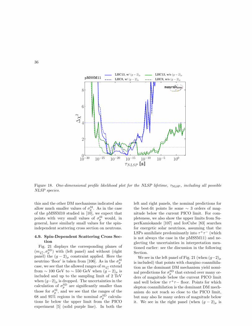
36

10−30 10−25 10−20 10−15 10−10 10−5 100

τNLSP [s]0

2

4

6

8

∆χ2


LHC8, w/ (g − 2)µ

LHC13, w/o (g − 2)µ

LHC8, w/o (g − 2)µ

Figure 18. One-dimensional profile likelihood plot for the NLSP lifetime, τNLSP, including all possibleNLSP species.

this and the other DM mechanisms indicated alsoallow much smaller values of σSI

p . As in the caseof the pMSSM10 studied in [10], we expect thatpoints with very small values of σSI

p would, ingeneral, have similarly small values for the spin-independent scattering cross section on neutrons.

4.9. Spin-Dependent Scattering Cross Sec-tion

Fig. 21 displays the corresponding planes of(mχ0

1, σSDp ) with (left panel) and without (right

panel) the (g − 2)µ constraint applied. Here theneutrino ‘floor’ is taken from [106]. As in the σSI

p

case, we see that the allowed ranges ofmχ01

extendfrom ∼ 100 GeV to ∼ 550 GeV when (g − 2)µ isincluded and up to the sampling limit of 2 TeVwhen (g−2)µ is dropped. The uncertainties in thecalculation of σSD

p are significantly smaller than

those for σSIp , and we see that the ranges of the

68 and 95% regions in the nominal σSDp calcula-

tions lie below the upper limit from the PICOexperiment [5] (solid purple line). In both the

left and right panels, the nominal predictions forthe best-fit points lie some ∼ 3 orders of mag-nitude below the current PICO limit. For com-pleteness, we also show the upper limits from Su-perKamiokande [107] and IceCube [83] searchesfor energetic solar neutrinos, assuming that theLSPs annihilate predominantly into τ+τ− (whichis not always the case in the pMSSM11) and ne-glecting the uncertainties in interpretation men-tioned earlier: see the discussion in the followingSection.

We see in the left panel of Fig. 21 (when (g−2)µis included) that points with chargino coannihila-tion as the dominant DM mechanism yield nomi-nal predictions for σSD

p that extend over many or-ders of magnitude below the current PICO limitand well below the τ+τ− floor. Points for whichslepton coannihilation is the dominant DM mech-anism do not reach so close to the PICO limit,but may also lie many orders of magnitude belowit. We see in the right panel (when (g − 2)µ is

37

10−7 10−5 10−3 10−1 101 103

τχ±1

[s]0

2

4

6

8

∆χ2


LHC8, w/ (g − 2)µ

LHC13, w/o (g − 2)µ

LHC8, w/o (g − 2)µ

10−7 10−5 10−3 10−1 101 103

ττ1[s]

0

2

4

6

8

∆χ2


LHC8, w/ (g − 2)µ

LHC13, w/o (g − 2)µ

LHC8, w/o (g − 2)µ

600 700 800 900 1000 1100 1200 1300 1400mχ±

1[GeV]

10−7

10−5

10−3

10−1

101

103

τ χ± 1

[s]


0 1000 2000 3000 4000mτ1

[GeV]10−7

10−5

10−3

10−1

101

103

τ τ1[s

]


Figure 19. Upper panels: one-dimensional profile likelihood plots for the lifetime of the χ±1 (left) and theτ1 (right). Lower panels: the corresponding mass-lifetime planes for the χ±1 and τ1, with the 95% CLregions shaded according to the dominant DM mechanisms.

38

100 101 102 103

mχ01[GeV]

10−50

10−48

10−46

10−44

10−42

10−40

10−38

σSI

p[c

m2]

PANDAX-II

XENON1T LUX

XENONnT

XENON1T

LZ

CRESST-II

CDMSliteCDEX-1


100 101 102 103

mχ01[GeV]

10−50

10−48

10−46

10−44

10−42

10−40

10−38

σSI

p[c

m2]

PANDAX-II

XENON1T LUX

XENONnT

XENON1T

LZ

CRESST-II

CDMSliteCDEX-1


±1 coann.




Figure 20. Planes of (mχ01, σSIp ) with (left panel) and without (right panel) the (g−2)µ constraint applied,

where the values of σSIp displayed are the nominal values calculated using the SSARD code. The upper

limits established by the LUX [4], XENON1T [6] and PandaX-II [3] Collaborations are shown as green,magenta and blue contours, respectively, and the combined limit is indicated by a black line with greenshading above. The projected future 90% CL exclusion sensitivities of the LUX-Zeplin (LZ) [104] andXENON1T/nT [105] experiments are shown as solid purple and dashed blue lines, respectively, and theneutrino background ‘floor’ is shown as a dashed light-blue line with a shading of the same colour below.

dropped) similar ranges of nominal σSDp values.

We also see that when mχ01& 1 TeV many com-

peting DM mechanisms come into play, and maygive small values of σSD

p . However, in the case

of squark coannihilation σSDp may lie within ∼ 3

orders of magnitude of the PICO upper limit.

4.10. Indirect Astrophysical Searches forDark Matter

We have explored the possible impact of indi-rect searches for DM via annihilations into neu-trinos inside the Sun. If the DM inside the Sun isin equilibrium between capture and annihilation,the annihilation is quadratically sensitive to thelocal Galactic DM density. However, as discussedearlier, equilibrium is not always a good approx-imation. We note also that the capture rate isnot determined solely by spin-dependent scatter-ing on protons in the Sun, but also depends onthe amount of spin-independent scattering on He-lium and heavy nuclei. As we have seen, the σSI

p

matrix element is more uncertain than that forσSDp , and this uncertainty should be propagated

into the constraint on σSDp . Finally, we note that

the greatest sensitivity of the IceCube search forenergetic neutrinos from the Sun [83] is for anni-hilations into τ+τ− and W+W−, which are notalways the dominant final states in the pMSSM11models of interest.

Using the nominal values of the matrix ele-ments from SSARD and neglecting the astrophys-ical uncertainties, we have calculated the sig-nals in the IceCube detector for a subset of ourpMSSM11 points that are consistent with thePICO constraint [5]. We find that the IceCubeW+W− constraint [83] has negligible impact onthese parameter sets, and that only a fraction areaffected by the IceCube τ+τ− constraint. In viewof this and the uncertainties in the interpretationof the IceCube searches, we have not includedthem in our fits.

39

100 101 102 103

mχ01[GeV]

10−47

10−45

10−43

10−41

10−39

10−37

σSD

p[cm

2]

PICO-60

Super-K (2016) τ τ

Super-K (2016) τ τ floor

IC (2016) τ τ

IC (2016) τ τ floor


100 101 102 103

mχ01[GeV]

10−47

10−45

10−43

10−41

10−39

10−37

σSD

p[cm

2]

PICO-60

Super-K (2016) τ τ

Super-K (2016) τ τ floor

IC (2016) τ τ

IC (2016) τ τ floor


±1 coann.




Figure 21. Planes of (mχ01, σSDp ) with (left panel) and without (right panel) the (g − 2)µ constraint

applied, where the values of σSDp displayed are the nominal values calculated using the SSARD code [43].

The upper limit established by the PICO Collaboration [5] is shown as a purple contour, with green shadingabove. The neutrino ‘floor’ for σSD

p is taken from [106]. We also show the indicative upper limits fromSuperKamiokande [107] and IceCube [83] searches for energetic solar neutrinos obtained assuming thatthe LSPs annihilate predominantly into τ+τ−, which are subject to the caveats discussed in the text.

5. Impacts of the LHC 13-TeV and NewDirect Detection Constraints

In this Section we illustrate the impact ofthe LHC 13-TeV data and the recent updatesfrom the Xenon-based direct detection experi-ments LUX, XENON1T, and PandaX-II [3, 4, 6]on relevant pMSSM11 parameter planes. In theleft panel of Fig. 22 we display the impact of thenew results on the (mq,mg) plane: the solid red,blue and green lines are the current 68%, 95%and 99.7% CL contours, and the dashed lines arethose for the corresponding 68, 95% and 99.7%CL contours in a global fit omitting the LHC 13-TeV constraints and those from the Xenon-baseddirect detection experiments. The right panel ofFig. 22 makes a similar comparison of the 68, 95and 99.7% CL regions in the (mχ0

1, σSIp ) plane

found in global fits including LHC 13-TeV andXenon-based detector data (solid lines) and omit-ting these data (dashed lines).

We see in the upper left panel of Fig. 22 thatthe LHC 13-TeV constraints exclude bands of pa-rameter space at low mq and mg, disallowingin particular a squark coannihilation region atmq ∼ 500 GeV and large mg and a gluino coan-nihilation strip at mg ∼ 500 GeV that were al-lowed by the LHC 8-TeV data. The impact on thegluino and squark coannihilation strips can alsobe appreciated from the upper right and lower leftpanels, where they appear as dashed-blue islandsalong the diagonal where the mass is degeneratewith the neutralino that disappear completely af-ter the inclusion of the LHC 13-TeV constraints.The bottom right panel of Fig. 22 shows that lowvalues of σSI

p that would have been allowed in afit without the LHC 13-TeV data are now disal-lowed. This effect is in addition to the downwardspressure on σSI

p exerted by the new generation ofXenon-based direct detection experiments.

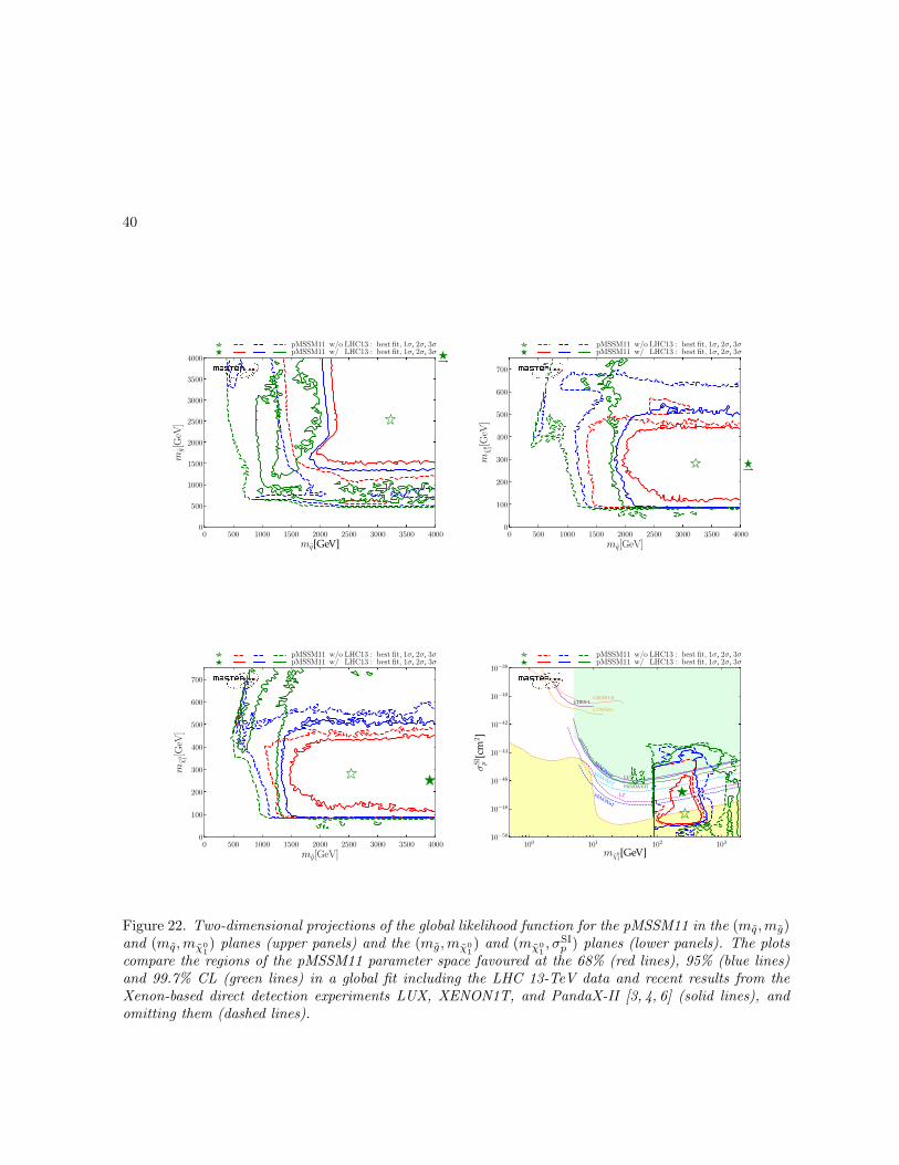
40

0 500 1000 1500 2000 2500 3000 3500 4000

mq[GeV]0

500

1000

1500

2000

2500

3000

3500

4000

mg[GeV

]

pMSSM11 w/ LHC13 : best fit, 1σ, 2σ, 3σpMSSM11 w/o LHC13 : best fit, 1σ, 2σ, 3σ

0 500 1000 1500 2000 2500 3000 3500 4000

mq[GeV]

0

100

200

300

400

500

600

700

mχ

0 1[GeV

]


0 500 1000 1500 2000 2500 3000 3500 4000

mg[GeV]

0

100

200

300

400

500

600

700

mχ

0 1[GeV

]


100 101 102 103

mχ01[GeV]

10−50

10−48

10−46

10−44

10−42

10−40

10−38

σSI

p[c

m2]

PANDAX-II

XENON1T LUX

XENONnT

XENON1T

LZ

CRESST-II

CDMSliteCDEX-1


Figure 22. Two-dimensional projections of the global likelihood function for the pMSSM11 in the (mq,mg)and (mq,mχ0

1) planes (upper panels) and the (mg,mχ0

1) and (mχ0

1, σSIp ) planes (lower panels). The plots

compare the regions of the pMSSM11 parameter space favoured at the 68% (red lines), 95% (blue lines)and 99.7% CL (green lines) in a global fit including the LHC 13-TeV data and recent results from theXenon-based direct detection experiments LUX, XENON1T, and PandaX-II [3, 4, 6] (solid lines), andomitting them (dashed lines).

41

6. Best-Fit Points, Spectra and Decays

Following our previous discussions of some two-dimensional projections of the pMSSM11 param-eter space and various one-dimension profile like-lihood functions, we now discuss in more de-tail the best-fit points in the pMSSM11 fits in-corporating the LHC 13-TeV data, both withand without the (g − 2)µ constraint, whose in-put pMSSM11 parameter values were given in thefirst and third columns of Table 4. We note, how-ever, that the likelihood functions are very flat forlarger masses, so these best-fit points should notbe taken as definite predictions.

Fig. 1 displays the spectra of Higgs bosons andsparticles at the best-fit points for the pMSSM11including (upper panel) and excluding (lowerpanel) the (g− 2)µ constraint 28. In each case wealso show the decay paths with branching ratios> 5%, the widths of the lines being proportionalto the branching ratios. The heavier Higgs bosonsH,A,H±, are lighter in the case without (g−2)µ,whereas the sleptons and the electroweak inos areheavier. The branching ratio patterns differ in thetwo cases, with the Higgs bosons mainly decayingto SM particles when (g−2)µ is not imposed. Wenote that the first- and second-generation slep-tons are much lighter than the third-generationsleptons in the case with (g − 2)µ. The third-generation squarks are also heavier when (g−2)µis dropped, whereas the gluino and the first- andsecond-generation squarks are lighter in this case.In both cases, the third-generation squarks maylie within reach of future LHC runs, whereas thefirst- and second generation squarks would be ac-cessible only if (g − 2)µ is dropped. The gluinowould also be accessible in this case, and possiblyalso if (g − 2)µ is included.

We re-emphasize that the remarks in the pre-vious paragraph apply to the best-fit points, andthat the spectra might differ significantly, as thelikelihood functions are quite flat for large masses.The 68 and 95% CL ranges are displayed inFig. 23 as orange and yellow bands, respectively,with the best-fit values indicated by blue lines.We see that for most sparticles the 95 and even68% CL ranges extend into the ranges accessible

28This figure was prepared using PySLHA [96].

to future LHC runs. As was to be expected, thebest prospects for measuring sparticles at a lineare+e− collider such as ILC [108,109] or CLIC [110]are offered by first- and second-generation slep-tons and the lighter electroweak inos χ0

1, χ02 and

χ±1 in the case with the (g − 2)µ constraint ap-plied.

Fig. 24 displays the breakdowns of the globalχ2 functions in the cases with (left panel) andwithout (right panel) the (g − 2)µ constraint 29.The different classes of observables are groupedtogether and colour-coded. We see that MW

makes only a small contribution, and that thetotal contribution to the global χ2 function ofthe precision electroweak observables are quitesimilar in the two cases. The total contributionof the flavour sector is slightly reduced when(g − 2)µ is dropped: ∆χ2 ∼ −1.2, largely be-cause of a better fit to BR(Bs → µ+µ−), butthis improvement is not very significant. Thecontributions of the Higgs, LEP, LHC and DMsectors are again very similar in the fits with andwithout (g − 2)µ.

7. Conclusions

In this paper we have used the MasterCode

tool to analyze the constraints on the parame-ter space of the pMSSM11 model, in which thesoft SUSY-breaking contributions to the massesof the first- and second-generation sleptons areallowed to vary independently from the third-generation slepton mass. We have taken into ac-count the available constraints on strongly- andelectroweakly-interacting sparticles from ∼ 36/fbof LHC data at 13 TeV [11–13] and the most re-cent limits from the LUX, PICO, XENON1T andPandaX-II experiments [3–6] searching directlyfor DM scattering. In addition, we have updatedthe constraint from the measurement of MW andsome constraints from flavour observables, as de-scribed in Table 2. We have presented the resultsfrom two global fits, one including the (g − 2)µconstraint and without it. We have also madevarious comparisons with fits without the LHC

29The corresponding horizontal bar has diagonal hatching,to recall that it is not included in the fit.

42

MhMHMAMH± mχ01mχ0

2mχ0

3mχ0

4mχ±1mχ±2 meL

meRmµL

mµRmτ1

mτ2mνemνµmντ mqL

mqRmt1

mt2mb1

mb2 mg0

1000

2000

3000

4000

Par

ticl

eM

asse

s[G

eV]

pMSSM11 w/ (g − 2)µ

MhMHMAMH± mχ01mχ0

2mχ0

3mχ0

4mχ±1mχ±2 meL

meRmµL

mµRmτ1

mτ2mνemνµmντ mqL

mqRmt1

mt2mb1

mb2 mg0

1000

2000

3000

4000

Par

ticl

eM

asse

s[G

eV]

pMSSM11 w/o (g − 2)µ

Figure 23. Higgs and sparticle spectrum for the pMSSM11 with and without the (g−2)µ constraint applied(upper and lower panels, respectively). The values at the best-fit points are indicated by blue lines, the68% CL ranges by orange bands, and the 95% CL ranges by yellow bands.

43

0 5 10 15

MZ

∆α(5)had(MZ)

Mt

MW

Ab

Ac

A0,bFB

A0,cFB

A0,lFB

Al(Pτ )

Al(SLD)

ΓZ

R0b

R0c

R0l

aEXPµ − aSMµ

σ0had

sin2 θleff(QhadFB )

BRB→Xsll

BRK→lν

BRK→πνν

BRB→Xsγ

BRB→τν

∆MBs

∆MBs

∆MBd

BRBs,d→µ+µ−

εk

∆χ2HiggsBounds

∆χ2HiggsSignals

Mh

LHC13 A/H

LEP

LHC8

LHC13 EWK

LHC13 color.

σSIp

ΩCDMh2

σSDp

65

(∆χ2)nuisance = 0.03

(∆χ2)EWPO = 16.88

(∆χ2)flavor = 4.48

(∆χ2)Higgs = 68.13

(∆χ2)LEP = 0.00

(∆χ2)LHC8 = 0.00

(∆χ2)LHC13 = 0.09

(∆χ2)DM = 0.52

∆χ2

0 5 10 15

MZ

∆α(5)had(MZ)

Mt

MW

Ab

Ac

A0,bFB

A0,cFB

A0,lFB

Al(Pτ )

Al(SLD)

ΓZ

R0b

R0c

R0l

aEXPµ − aSMµ

σ0had

sin2 θleff(QhadFB )

BRB→Xsll

BRK→lν

BRK→πνν

BRB→Xsγ

BRB→τν

∆MBs

∆MBs

∆MBd

BRBs,d→µ+µ−

εk

∆χ2HiggsBounds

∆χ2HiggsSignals

Mh

LHC13 A/H

LEP

LHC8

LHC13 color.

LHC13 EWK

σSIp

ΩCDMh2

σSDp

65

(∆χ2)nuisance = 0.05

(∆χ2)EWPO = 16.72

(∆χ2)flavor = 3.97

(∆χ2)Higgs = 68.08

(∆χ2)LEP = 0.00

(∆χ2)LHC8 = 0.00

(∆χ2)LHC13 = 0.04

(∆χ2)DM = 0.06

∆χ2

Figure 24. The χ2 pulls at the best-fit points in the pMSSM11 including (left) and without the (g − 2)µconstraint (right). In the rightmost plot, the χ2 pull from (g− 2)µ is shown (hatched orange bar), but itspenalty is not included in the fit.

44

13-TeV data. Comparing with our earlier fit tothe pMSSM10 [10], we note that the freedom form˜ 6= mτ plays an important role in best fits.Furthermore, there is a big difference betweenM1 and M2 at the best-fit point without (g−2)µ.

The most visible impact of the LHC 13-TeV constraints has been on the masses of thestrongly-interacting sparticles: see the left pan-els of Figs. 8 and 9 and compare the solid anddashed curves. On the other hand, the impactof the LHC constraints on electroweak inos hasbeen less marked: see Fig. 11. As was to be ex-pected, the importance of the (g− 2)µ constraintis seen in the likelihood functions for charged slep-ton masses and electroweak inos: compare theblue and green curves in Figs. 10 and 11. Thecomposition of the LSP χ0

1 is also different in thecases with and without (g−2)µ: as seen in Fig. 12

and Table 6, a B LSP is preferred when (g − 2)µis included, whereas a H LSP is preferred when(g − 2)µ is dropped. Moreover, the inclusion ofthe (g−2)µ constraint also has significant indirectimplications for the squark masses, as also seen inFigs. 8 and 9. This analysis reinforces the impor-tance of clarifying the interpretation of the dif-ference between the experimental measurementand the SM calculation of (g− 2)µ. We thereforewelcome the advent of the Fermilab (g − 2)µ ex-periment [111] and continued efforts to refine theSM calculation.

We have also analyzed in this paper the im-portances of different mechanisms for bringingthe relic LSP density into the range favoured byPlanck 2015 and other data: see the shadings inFigs. 2, 4, 5, 6, 19, 20 and 21, and the profile χ2

functions for the DM measures in Fig. 17. As wesee there, important roles are played by charginocoannihilation, slepton coannihilation and rapidannihilation via direct-channel H/A boson ex-change, though other mechanisms such as stauand squark coannihilation may be important inlimited regions of parameter space 30. In the case

30Compared to the pMSSM7 analysis in [24], we find thatstop coannihilation is less prominent, and that rapid an-nihilation through the Z and the light Higgs boson is ofvery limited importance. In these respects the more gen-eral realization of the MSSM with four additional free pa-rameters yields substantially different results.

where the (g − 2)µ constraint is dropped, thereis a preference for a region where mχ0

1∼ mχ±

1∼

mq ∼ mg where multiple coannihilation processesplay a role, and the compressed spectrum reducesthe sensitivity of the LHC sparticle searches.

In general, our analysis favours quite small de-viations from the SM predictions for electroweak,flavour and Higgs observables: see Figs. 12 and14, in particular. We have also analyzed thepMSSM11 predictions for the A∆Γ and τ(Bs →µ+µ−) observables recently measured for the firsttime by the LHCb Collaboration [57]. As seen inFig. 13, the pMSSM11 predictions for these ob-servables are very similar to those in the SM, de-viating by much less than the current experimen-tal uncertainties. Accordingly, we do not includeA∆Γ and τ(Bs → µ+µ−) in our global fits.

We find that current LHC searches for long-lived particles do not impact our scan of thepMSSM11 parameter space. However, thepMSSM11 still offers significant prospects for thediscovery of long-lived particles. When the (g −2)µ constraint is imposed, we find that ∆χ2 & 4for τNLSP & 10−10 s. However, when the (g− 2)µconstraint is dropped, values of τNLSP as long as103 s (the limit we impose in order to maintainsuccessful Big Bang nucleosynthesis) are allowedat the ∆χ2 . 4 level,

As seen in Figs. 20 and 21, the pMSSM11 of-fers interesting prospects for the detection of su-persymmetric DM. In both the spin-independentand -dependent cases, cross sections close to thepresent experimental upper limits are favoured atthe 68% CL, whether or not (g−2)µ is included inthe set of constraints. Interestingly, in the caseof σSI

p with (g − 2)µ included, there is a lowerlimit that is not far below the neutrino ‘floor’ 31,whereas σSI

p may be much lower when (g − 2)µis dropped, and low values of σSD

p are allowed inboth cases.

We turn finally to the prospects for discov-ering sparticles in future runs of the LHC, orwith a future linear e+e− collider. As seen inFig. 21, whether or not (g − 2)µ is included in

31However, we repeat that the uncertainties in the calcu-lation of σSI

p are large, and these remarks apply within the

framework of a calculation of σSIp using SSARD.

45

the global fit, the third-generation squarks maywell be within reach of future LHC runs, andthe first- and second-generation squarks and thegluino may also be accessible if the (g − 2)µ con-straint is dropped. If it is included, on the otherhand, there are also good prospects for discov-ering electroweakly-interacting sparticles at ane+e− collider, in particular the e, µ, χ0

1, χ02 and

χ±1 .It is often said that the night is darkest just

before dawn, and the same may be true for su-persymmetry.

Acknowledgements

We thank Gino Isidori for useful discussions.The work of E.B. and G.W. is supported in partby the Collaborative Research Center SFB676 ofthe DFG, “Particles, Strings and the early Uni-verse”. The work of K.S. is partially supportedby the National Science Centre, Poland, un-der research grants DEC-2014/15/B/ST2/02157,DEC-2015/18/M/ST2/00054 and DEC-2015/19/D/ST2/03136. K.S. thanks the TUMunich for hospitality during the final stages ofthis work and has been partially supported bythe DFG cluster of excellence EXC 153 “Originand Structure of the Universe”, by the Collab-orative Research Center SFB1258. The work ofM.B., I.S.F. and D.M.S. is supported by the Eu-ropean Research Council via Grant BSMFLEET639068. The work of J.C.C. is supported byCNPq (Brazil). The work of M.J.D. is supportedin part by the Australia Research Council. Thework of J.E. is supported in part by STFC (UK)via the research grant ST/L000326/1 and in partvia the Estonian Research Council via a Mobil-itas Pluss grant, and the work of H.F. is alsosupported in part by STFC (UK). The workof S.H. is supported in part by the MEINCOPSpain under contract FPA2016-78022-P, in partby the Spanish Agencia Estatal de Investigacion(AEI) and the EU Fondo Europeo de Desar-rollo Regional (FEDER) through the projectFPA2016-78645-P, in part by the AEI throughthe grant IFT Centro de Excelencia Severo OchoaSEV-2016-0597, and by the Spanish MICINNConsolider-Ingenio 2010 Program under Grant

MultiDark CSD2009-00064. The work of M.L.and I.S.F. is supported by XuntaGal. The workof K.A.O. is supported in part by DOE grant de-sc0011842 at the University of Minnesota. Thework of G.W. is also supported in part by theEuropean Commission through the “HiggsTools”Initial Training Network PITN-GA-2012-316704.During part of this work we used the middle-ware suite udocker [112] to deploy MasterCode

on clusters, developed by the EC H2020 projectINDIGO-Datacloud (RIA 653549). We are par-ticularly grateful to Jorge Gomes for his kindsupport. We also thank DESY and especiallythe DESY IT department for making us availablethe computational resources of the BIRD/NAF2cluster, which have been used intensively to carryout this work.

REFERENCES

1. For a compendium of CMSsearches for supersymmetry, seehttps://twiki.cern.ch/twiki/bin/view/

CMSPublic/PhysicsResultsSUS.2. For a compendium of ATLAS

searches for supersymmetry, seehttps://twiki.cern.ch/twiki/bin/view/

AtlasPublic/SupersymmetryPublicResults.3. X. Cui et al. [PandaX-II Collaboration],

arXiv:1708.06917 [hep-ex], which updatesA. Tan et al. [PandaX-II Collaboration],Phys. Rev. Lett. 117 (2016) no. 12, 121303[arXiv:1607.07400 [hep-ex]].

4. D. S. Akerib et al. [LUX Collaboration],Phys. Rev. Lett. 118 (2017) no.2, 021303[arXiv:1608.07648 [astro-ph.CO]].

5. C. Amole et al. [PICO Collaboration],arXiv:1702.07666 [astro-ph.CO].

6. E. Aprile et al. [XENON Collaboration],arXiv:1705.06655 [astro-ph.CO].

7. O. Buchmueller et al., Phys. Lett. B 657(2007) 87 doi:10.1016/j.physletb.2007.09.058[arXiv:0707.3447 [hep-ph]]; Eur. Phys. J.C 72 (2012) 1878 [arXiv:1110.3568 [hep-ph]]; Eur. Phys. J. C 72 (2012) 2243[arXiv:1207.7315]; Eur. Phys. J. C 74 (2014)2809 [arXiv:1312.5233 [hep-ph]].

8. O. Buchmueller et al., Eur. Phys. J. C 74

http://arxiv.org/abs/de-sc/0011842

http://arxiv.org/abs/de-sc/0011842

http://arxiv.org/abs/1708.06917









46

(2014) 2922 [arXiv:1312.5250 [hep-ph]].9. O. Buchmueller et al., Eur. Phys. J. C 74

(2014) 12, 3212 [arXiv:1408.4060 [hep-ph]].10. K. J. de Vries et al., Eur. Phys. J. C 75 (2015)

no.9, 422 [arXiv:1504.03260 [hep-ph]].11. A. M. Sirunyan et al. [CMS Collaboration],

arXiv:1705.04650 [hep-ex].12. A. M. Sirunyan et al. [CMS Collaboration],

arXiv:1705.04673 [hep-ex].13. A. M. Sirunyan et al. [CMS Collaboration],

arXiv:1709.05406 [hep-ex].14. J. Billard, L. Strigari and E. Figueroa-

Feliciano, Phys. Rev. D 89 (2014) no.2,023524 doi:10.1103/PhysRevD.89.023524[arXiv:1307.5458 [hep-ph]]; P. Cushman,C. Galbiati, D. N. McKinsey, H. Robert-son, T. M. P. Tait, D. Bauer, A. Borglandand B. Cabrera et al., Snowmass WorkingGroup Report: WIMP Dark Matter DirectDetection, arXiv:1310.8327 [hep-ex].

15. H. Goldberg, Phys. Rev. Lett. 50 (1983) 1419;J. Ellis, J. Hagelin, D. Nanopoulos, K. Oliveand M. Srednicki, Nucl. Phys. B 238 (1984)453.

16. G. Bertone, D. G. Cerdeno, M. For-nasa, R. Ruiz de Austri, C. Stregeand R. Trotta, JCAP 1201 (2012)015 doi:10.1088/1475-7516/2012/01/015[arXiv:1107.1715 [hep-ph]]; A. Fowlie,A. Kalinowski, M. Kazana, L. Roszkowskiand Y. L. S. Tsai, Phys. Rev. D 85 (2012)075012 doi:10.1103/PhysRevD.85.075012[arXiv:1111.6098 [hep-ph]]; C. Strege,G. Bertone, D. G. Cerdeno, M. For-nasa, R. Ruiz de Austri and R. Trotta,JCAP 1203 (2012) 030 doi:10.1088/1475-7516/2012/03/030 [arXiv:1112.4192 [hep-ph]]; L. Roszkowski, E. M. Sessolo andY. L. S. Tsai, Phys. Rev. D 86 (2012)095005 doi:10.1103/PhysRevD.86.095005[arXiv:1202.1503 [hep-ph]]; P. Bech-tle et al., JHEP 1206 (2012)098 doi:10.1007/JHEP06(2012)098[arXiv:1204.4199 [hep-ph]]; A. Fowlie,M. Kazana, K. Kowalska, S. Munir,L. Roszkowski, E. M. Sessolo, S. Trojanowskiand Y. L. S. Tsai, Phys. Rev. D 86 (2012)075010 doi:10.1103/PhysRevD.86.075010

[arXiv:1206.0264 [hep-ph]]; K. Kowal-ska, S. Munir, L. Roszkowski,E. M. Sessolo, S. Trojanowski andY. L. S. Tsai, Phys. Rev. D 87 (2013)115010 doi:10.1103/PhysRevD.87.115010[arXiv:1211.1693 [hep-ph]]; C. Strege,G. Bertone, F. Feroz, M. Fornasa, R. Ruizde Austri and R. Trotta, JCAP 1304 (2013)013 doi:10.1088/1475-7516/2013/04/013[arXiv:1212.2636 [hep-ph]]; L. Roszkowski,E. M. Sessolo and A. J. Williams, JHEP 1408(2014) 067 doi:10.1007/JHEP08(2014)067[arXiv:1405.4289 [hep-ph]]; P. Bechtleet al., Eur. Phys. J. C 76 (2016) no.2,96 doi:10.1140/epjc/s10052-015-3864-0 [arXiv:1508.05951 [hep-ph]]; C. Han,K. i. Hikasa, L. Wu, J. M. Yang andY. Zhang, Phys. Lett. B 769 (2017)470 doi:10.1016/j.physletb.2017.04.026[arXiv:1612.02296 [hep-ph]].

17. P. Athron et al. [GAMBIT Collaboration],arXiv:1705.07935 [hep-ph].

18. E. Bagnaschi et al., Eur. Phys. J. C 77 (2017)no.4, 268 [arXiv:1612.05210 [hep-ph]].

19. E. Bagnaschi et al., Eur. Phys. J. C 77 (2017)no.2, 104 [arXiv:1610.10084 [hep-ph]].

20. See, for example, C. F. Berger, J. S. Gainer,J. L. Hewett and T. G. Rizzo, JHEP0902, 023 (2009) [arXiv:0812.0980 [hep-ph]]; S. S. AbdusSalam, B. C. Allanach,F. Quevedo, F. Feroz and M. Hobson, Phys.Rev. D 81, 095012 (2010) [arXiv:0904.2548[hep-ph]]; J. A. Conley, J. S. Gainer,J. L. Hewett, M. P. Le and T. G. Rizzo, Eur.Phys. J. C 71, 1697 (2011) [arXiv:1009.2539[hep-ph]]; J. A. Conley, J. S. Gainer,J. L. Hewett, M. P. Le and T. G. Rizzo,[arXiv:1103.1697 [hep-ph]]; S. S. Abdus-Salam, et al., Eur. Phys. J. C 71 (2011)1835 [arXiv:1109.3859 [hep-ph]]; S. Sek-men, S. Kraml, J. Lykken, F. Moort-gat, S. Padhi, L. Pape, M. Pierini andH. B. Prosper et al., JHEP 1202 (2012)075 [arXiv:1109.5119 [hep-ph]]; A. Arbey,M. Battaglia and F. Mahmoudi, Eur. Phys.J. C 72 (2012) 1847 [arXiv:1110.3726 [hep-ph]]; A. Arbey, M. Battaglia, A. Djouadiand F. Mahmoudi, Phys. Lett. B 720 (2013)






























47

153 [arXiv:1211.4004 [hep-ph]]; M. W. Cahill-Rowley, J. L. Hewett, A. Ismail andT. G. Rizzo, Phys. Rev. D 88 (2013) 3, 035002[arXiv:1211.1981 [hep-ph]].

21. A. Fowlie, K. Kowalska, L. Roszkowski,E. M. Sessolo and Y. L. S. Tsai,Phys. Rev. D 88 (2013) 055012doi:10.1103/PhysRevD.88.055012[arXiv:1306.1567 [hep-ph]]; C. Strege,G. Bertone, G. J. Besjes, S. Caron, R. Ruiz deAustri, A. Strubig and R. Trotta, JHEP 1409(2014) 081 doi:10.1007/JHEP09(2014)081[arXiv:1405.0622 [hep-ph]]; M. Cahill-Rowley,J. L. Hewett, A. Ismail and T. G. Rizzo,Phys. Rev. D 91 (2015) no.5, 055002[arXiv:1407.4130 [hep-ph]]; L. Roszkowski,E. M. Sessolo and A. J. Williams, JHEP 1502(2015) 014 doi:10.1007/JHEP02(2015)014[arXiv:1411.5214 [hep-ph]]; G. Bertone,F. Calore, S. Caron, R. Ruiz, J. S. Kim,R. Trotta and C. Weniger, JCAP 1604(2016) no.04, 037 doi:10.1088/1475-7516/2016/04/037 [arXiv:1507.07008 [hep-ph]].

22. R. K. Barman, B. Bhattacherjee, A. Choud-hury, D. Chowdhury, J. Lahiri andS. Ray, arXiv:1608.02573 [hep-ph];C. Boehm, P. S. B. Dev, A. Mazum-dar and E. Pukartas, JHEP 1306(2013) 113 doi:10.1007/JHEP06(2013)113[arXiv:1303.5386 [hep-ph]].

23. E. A. Bagnaschi et al., Eur. Phys. J. C 75(2015) 500 [arXiv:1508.01173 [hep-ph]].

24. P. Athron et al. [GAMBIT Collaboration],arXiv:1705.07917 [hep-ph].

25. J. Ellis, F. Luo and K. A. Olive, JHEP 1509(2015) 127 [arXiv:1503.07142 [hep-ph]].

26. J. Ellis, J. L. Evans, F. Luo and K. A. Olive,JHEP 1602 (2016) 071 [arXiv:1510.03498[hep-ph]].

27. [ATLAS and CDF and CMS and D0 Collab-orations], arXiv:1403.4427 [hep-ex].

28. K. A. Olive et al. [Particle Data Group], Chin.Phys. C 38 (2014) 090001. doi:10.1088/1674-1137/38/9/090001

29. F. Feroz and M.P. Hobson,Mon. Not. Roy. Astron. Soc. 384(2008) 449 [arXiv:0704.3704 [astro-ph]].

F. Feroz, M.P. Hobson and M. Bridges,Mon. Not. Roy. Astron. Soc. 398 (2009)1601-1614 [arXiv:0809.3437 [astro-ph]].F. Feroz, M.P. Hobson, E. Cameron andA.N. Pettitt, [arXiv:1306.2144 [astro-ph]].

30. For more information and updates, please seehttp://cern.ch/mastercode/. A survey ofLHC Run 1 constraints can be found in K. J.de Vries, Global Supersymmetric Models afterLHC Fits of Run 1 (PhD thesis, 2015), avail-able on this website.

31. P. Skands et al., JHEP 0407 (2004) 036[arXiv:hep-ph/0311123];

32. B. C. Allanach, Comput. Phys. Commun. 143(2002) 305 [arXiv:hep-ph/0104145].

33. S. Heinemeyer et al., JHEP 0608 (2006)052 [arXiv:hep-ph/0604147]; S. Heinemeyer,W. Hollik, A. M. Weber and G. Weiglein,JHEP 0804 (2008) 039 [arXiv:0710.2972[hep-ph]].

34. S. Heinemeyer, W. Hollik, G. Wei-glein and L. Zeune, JHEP 1312 (2013)084 doi:10.1007/JHEP12(2013)084[arXiv:1311.1663 [hep-ph]].

35. S. Heinemeyer, W. Hollik and G. Wei-glein, Comput. Phys. Commun. 124 (2000)76 [arXiv:hep-ph/9812320]; S. Heinemeyer,W. Hollik and G. Weiglein, Eur. Phys.J. C 9 (1999) 343 [arXiv:hep-ph/9812472];G. Degrassi, S. Heinemeyer, W. Hollik,P. Slavich and G. Weiglein, Eur. Phys. J.C 28 (2003) 133 [arXiv:hep-ph/0212020];M. Frank et al., JHEP 0702 (2007) 047[arXiv:hep-ph/0611326]; T. Hahn, S. Heine-meyer, W. Hollik, H. Rzehak and G. Weiglein,Comput. Phys. Commun. 180 (2009) 1426;T. Hahn, S. Heinemeyer, W. Hollik, H. Rze-hak and G. Weiglein, Phys. Rev. Lett. 112(2014) 14, 141801 [arXiv:1312.4937 [hep-ph]];See http://www.feynhiggs.de .

36. P. Athron, J. h. Park, D. Stkinger andA. Voigt, Comput. Phys. Commun. 190(2015) 139 [arXiv:1406.2319 [hep-ph]].

37. P. Athron, M. Bach, D. Harries, T. Kwas-nitza, J. h. Park, D. Stckinger, A. Voigtand J. Ziebell, arXiv:1710.03760 [hep-ph]; E. Bagnaschi, G. F. Giudice,P. Slavich and A. Strumia, JHEP 1409


















http://cern.ch/mastercode/

http://arxiv.org/abs/hep-ph/0311123










http://www.feynhiggs.de



48

(2014) 092 doi:10.1007/JHEP09(2014)092[arXiv:1407.4081 [hep-ph]]; E. Bagnaschi,J. Pardo Vega and P. Slavich, Eur. Phys. J. C77 (2017) no.5, 334 doi:10.1140/epjc/s10052-017-4885-7 [arXiv:1703.08166 [hep-ph]].

38. P. Athron, J. h. Park, T. Steudtner,D. Stckinger and A. Voigt, JHEP 1701(2017) 079 doi:10.1007/JHEP01(2017)079[arXiv:1609.00371 [hep-ph]].

39. H. Bahl and W. Hollik, Eur. Phys. J. C76 (2016) 499 [arXiv:1608.01880 [hep-ph]];H. Bahl, S. Heinemeyer, W. Hollik andG. Weiglein, arXiv:1706.00346 [hep-ph].

40. G. Isidori and P. Paradisi, Phys. Lett.B 639 (2006) 499 [arXiv:hep-ph/0605012];G. Isidori, F. Mescia, P. Paradisi andD. Temes, Phys. Rev. D 75 (2007)115019 [arXiv:hep-ph/0703035], and refer-ences therein.

41. F. Mahmoudi, Comput. Phys. Commun.178 (2008) 745 [arXiv:0710.2067 [hep-ph]];Comput. Phys. Commun. 180 (2009) 1579[arXiv:0808.3144 [hep-ph]]; D. Eriksson,F. Mahmoudi and O. Stal, JHEP 0811 (2008)035 [arXiv:0808.3551 [hep-ph]].

42. G. Belanger, F. Boudjema, A. Pukhov andA. Semenov, Comput. Phys. Commun. 185(2014) 960 [arXiv:1305.0237 [hep-ph]], andreferences therein.

43. Information about this code is available fromK. A. Olive: it contains important contribu-tions from J. Evans, T. Falk, A. Ferstl, G. Ga-nis, F. Luo, A. Mustafayev, J. McDonald, F.Luo, K. A. Olive, P. Sandick, Y. Santoso,C. Savage, V. Spanos and M. Srednicki.

44. J. R. Ellis, A. Ferstl and K. A. Olive, Phys.Lett. B 481, 304 (2000) doi:10.1016/S0370-2693(00)00459-7 [hep-ph/0001005];J. R. Ellis, K. A. Olive, Y. Santoso andV. C. Spanos, Phys. Rev. D 71, 095007(2005) doi:10.1103/PhysRevD.71.095007[hep-ph/0502001].

45. J. R. Ellis, K. A. Olive and C. Savage, Phys.Rev. D 77 (2008) 065026 [arXiv:0801.3656[hep-ph]].

46. M. Muhlleitner, A. Djouadi and Y. Mambrini,Comput. Phys. Commun. 168 (2005) 46 [hep-ph/0311167].

47. P. Bechtle, S. Heinemeyer, O. Stal, T. Ste-faniak and G. Weiglein, Eur. Phys. J. C74 (2014) 2, 2711 [arXiv:1305.1933 [hep-ph]]; JHEP 1411 (2014) 039 [arXiv:1403.1582[hep-ph]].

48. P. Bechtle, O. Brein, S. Heinemeyer,G. Weiglein and K. E. Williams, Com-put. Phys. Commun. 181 (2010) 138[arXiv:0811.4169 [hep-ph]], Comput. Phys.Commun. 182 (2011) 2605 [arXiv:1102.1898[hep-ph]]; P. Bechtle et al., Eur. Phys. J. C74 (2014) 3, 2693 [arXiv:1311.0055 [hep-ph]];P. Bechtle, S. Heinemeyer, O. Stal, T. Ste-faniak and G. Weiglein, Eur. Phys. J. C 75(2015) no.9, 421 [arXiv:1507.06706 [hep-ph]].

49. J. de Blas [HEPFit Collabora-tion], talk given at the First FCCPhysics Workshop, CERN, Jan. 2017,https://indico.cern.ch/event/550509/

contributions/2413788/attachments/

1396663/2130440/1stFCC Ph W deBlas.pdf.50. P. Athron et al., Eur. Phys. J. C 76 (2016)

no.2, 62 doi:10.1140/epjc/s10052-015-3870-2[arXiv:1510.08071 [hep-ph]].

51. LEP Electroweak Working Group [ALEPH,CDF, D0, DELPHI, L3, OPAL and SLDCollaborations, LEP Electroweak WorkingGroup, Tevatron Electroweak Working Groupand SLD Electroweak and Heavy FlavourGroups], arXiv:1012.2367 [hep-ex].

52. M. Baak [Gfitter Collaboration], PoS EPS -HEP2013 (2013) 203.

53. D. Stockinger, J. Phys. G 34 (2007)R45 [arXiv:hep-ph/0609168]; J. Miller,E. de Rafael and B. Roberts, Rept. Prog.Phys. 70 (2007) 795 [arXiv:hep-ph/0703049];J. Prades, E. de Rafael and A. Vainshtein,arXiv:0901.0306 [hep-ph]; F. Jegerlehnerand A. Nyffeler, Phys. Rept. 477, 1 (2009)[arXiv:0902.3360 [hep-ph]]; M. Davier,A. Hoecker, B. Malaescu, C. Z. Yuan andZ. Zhang, Eur. Phys. J. C 66, 1 (2010)[arXiv:0908.4300 [hep-ph]]. J. Prades,Acta Phys. Polon. Supp. 3, 75 (2010)[arXiv:0909.2546 [hep-ph]]; T. Teubner,K. Hagiwara, R. Liao, A. D. Martin andD. Nomura, arXiv:1001.5401 [hep-ph];M. Davier, A. Hoecker, B. Malaescu and
































49

Z. Zhang, Eur. Phys. J. C 71 (2011) 1515[arXiv:1010.4180 [hep-ph]].

54. G. Bennett et al. [The Muon g-2 Collabo-ration], Phys. Rev. Lett. 92 (2004) 161802,[arXiv:hep-ex/0401008]; and Phys. Rev. D 73(2006) 072003 [arXiv:hep-ex/0602035].

55. V. Khachatryan et al. [CMS and LHCbCollaborations], Nature 522 (2015) 68[arXiv:1411.4413 [hep-ex]]

56. M. Aaboud et al. [ATLAS Collaboration],Eur. Phys. J. C 76 (2016) no.9, 513[arXiv:1604.04263 [hep-ex]].

57. R. Aaij et al. [LHCb Collaboration], Phys.Rev. Lett. 118 (2017) no.19, 191801[arXiv:1703.05747 [hep-ex]].

58. M. Misiak, H. M. Asatrian, R. Boughezal,M. Czakon, T. Ewerth, A. Ferroglia,P. Fiedler and P. GamBino et al.,arXiv:1503.01789 [hep-ph].

59. Y. Amhis et al. [Heavy Flavor Aver-aging Group (HFAG) Collaboration],arXiv:1412.7515 [hep-ex].

60. B. Kronenbitter et al. [Belle Collabora-tion], Phys. Rev. D 92 (2015) no.5, 051102[arXiv:1503.05613 [hep-ex]].

61. T. Huber, T. Hurth and E. Lunghi, JHEP1506 (2015) 176 [arXiv:1503.04849 [hep-ph]].

62. A. J. Buras, P. GamBino, M. Gorbahn,S. Jager and L. Silvestrini, Nucl. Phys. B 592(2001) 55 [hep-ph/0007313].

63. W. J. Marciano, Phys. Rev. Lett. 93 (2004)231803 [arXiv:hep-ph/0402299].

64. C. Patrignani et al. [Particle Data Group],Chin. Phys. C 40 (2016) no.10, 100001 and2017 update.

65. A. J. Buras, D. Buttazzo, J. Girrbach-Noeand R. Knegjens, JHEP 1511 (2015) 033[arXiv:1503.02693 [hep-ph]].

66. A. V. Artamonov et al. [E949 Collabora-tion], Phys. Rev. Lett. 101 (2008) 191802[arXiv:0808.2459 [hep-ex]].

67. CMS Collaboration [CMS Collaboration],CMS-PAS-EXO-16-036.

68. V. Khachatryan et al. [CMS Collabora-tion], Eur. Phys. J. C 75 (2015) no.7, 325[arXiv:1502.02522 [hep-ex]].

69. V. Khachatryan et al. [ CMS Collaboration],JHEP 1410 (2014) 160 [arXiv:1408.3316

[hep-ex]].70. P. Bechtle, S. Heinemeyer, O. Stal, T. Ste-

faniak and G. Weiglein, Eur. Phys. J. C 75(2015) 9, 421 [arXiv:1507.06706 [hep-ph]].

71. The ATLAS collaboration [ATLAS Collabo-ration], ATLAS-CONF-2016-085.

72. ATLAS Collaboration,http://cds.cern.ch/record/2273866/

files/ATLAS-CONF-2017-050.pdf.73. P. A. R. Ade et al. [Planck Collabora-

tion], Astron. Astrophys. 594 (2016) A13[arXiv:1502.01589 [astro-ph.CO]].

74. B. Borasoy and U. G. Meissner, Annals Phys.254 (1997) 192 [hep-ph/9607432].

75. J. M. Alarcon, L. S. Geng, J. Martin Ca-malich and J. A. Oller, Phys. Lett. B 730(2014) 342 [arXiv:1209.2870 [hep-ph]].

76. X. Z. Ling, X. L. Ren and L. S. Geng,arXiv:1710.07164 [hep-ph].

77. M. Hoferichter, J. Ruiz de Elvira, B. Kubisand U. G. Mei?ner, Phys. Rev. Lett. 115(2015) 092301 [arXiv:1506.04142 [hep-ph]].

78. J. Ruiz de Elvira, M. Hoferichter, B. Kubisand U. G. Meissner, arXiv:1706.01465 [hep-ph].

79. J. M. Alarcon, J. Martin Camalich andJ. A. Oller, Phys. Rev. D 85 (2012) 051503[arXiv:1110.3797 [hep-ph]].

80. R. D. Young and A. W. Thomas,Phys. Rev. D 81 (2010) 014503doi:10.1103/PhysRevD.81.014503[arXiv:0901.3310 [hep-lat]]; J. Giedt,A. W. Thomas and R. D. Young,Phys. Rev. Lett. 103 (2009) 201802doi:10.1103/PhysRevLett.103.201802[arXiv:0907.4177 [hep-ph]]; H. W. Lin,arXiv:1112.2435 [hep-lat]; L. Alvarez-Ruso, T. Ledwig, J. Martin Ca-malich and M. J. Vicente-Vacas,Phys. Rev. D 88 (2013) no.5, 054507doi:10.1103/PhysRevD.88.054507[arXiv:1304.0483 [hep-ph]].

81. J. R. Ellis, R. A. Flores and S. Ritz, Phys.Lett. B 198 (1987) 393.

82. J. Ellis, K. A. Olive and V. C. Spanos, JCAP1110 (2011) 024 [arXiv:1106.0768 [hep-ph]].

83. M. G. Aartsen et al. [IceCube Collabora-tion], Eur. Phys. J. C 77 (2017) no.3, 146


http://arxiv.org/abs/hep-ex/0401008

http://arxiv.org/abs/hep-ex/0602035















http://cds.cern.ch/record/2273866/













50

[arXiv:1612.05949 [astro-ph.HE]].84. J. Ellis, K. A. Olive, C. Savage and

V. C. Spanos, Phys. Rev. D 81 (2010) 085004[arXiv:0912.3137 [hep-ph]].

85. M. Drees, H. Dreiner, D. Schmeier, J. Tatter-sall and J. S. Kim, Comput. Phys. Commun.187 (2015) 227 [arXiv:1312.2591 [hep-ph]].

86. C. Bals et al. [GAMBIT Collaboration],Eur. Phys. J. C 77 (2017) no.11, 795[arXiv:1705.07919 [hep-ph]].

87. E. Conte, B. Fuks and G. Serret, Com-put. Phys. Commun. 184 (2013) 222[arXiv:1206.1599 [hep-ph]].

88. M. Papucci, K. Sakurai, A. Weiler and L. Ze-une, Eur. Phys. J. C 74 (2014) no.11, 3163[arXiv:1402.0492 [hep-ph]].

89. S. Kraml, S. Kulkarni, U. Laa, A. Lessa,W. Magerl, D. Proschofsky-Spindler andW. Waltenberger, Eur. Phys. J. C 74 (2014)2868 [arXiv:1312.4175 [hep-ph]].

90. F. Ambrogi et al., arXiv:1701.06586 [hep-ph].91. W. Beenakker, C. Borschensky, M. Krmer,

A. Kulesza, E. Laenen, S. Marzani andJ. Rojo, Eur. Phys. J. C 76 (2016) no.2, 53[arXiv:1510.00375 [hep-ph]]; W. Beenakker,M. Kramer, T. Plehn, M. Spira and P. M. Zer-was, Nucl. Phys. B 515 (1998) 3 [hep-ph/9710451];

92. E. A. Bagnaschi, M. Papucci, K. Sakurai,A. Weiler and L. Zeune, in preparation.

93. G. Aad et al. [ATLAS and CMS Collabora-tions], JHEP 1608 (2016) 045[arXiv:1606.02266 [hep-ex]].

94. CMS Collaboration, CMS-PAS-EXO-16-036.95. T. Jittoh, K. Kohri, M. Koike, J. Sato, T. Shi-

momura and M. Yamanaka, Phys. Rev. D76 (2007) 125023 [arXiv:0704.2914 [hep-ph]];K. Jedamzik, Phys. Rev. D 77 (2008) 063524[arXiv:0707.2070 [astro-ph]] and JCAP 0803(2008) 008 [arXiv:0710.5153 [hep-ph]]; T. Jit-toh, K. Kohri, M. Koike, J. Sato, T. Shi-momura and M. Yamanaka, Phys. Rev. D78 (2008) 055007 [arXiv:0805.3389 [hep-ph]];T. Jittoh, K. Kohri, M. Koike, J. Sato,K. Sugai, M. Yamanaka and K. Yazaki, Phys.Rev. D 84 (2011) 035008 [arXiv:1105.1431[hep-ph]]; R. H. Cyburt, J. Ellis, B. D. Fields,F. Luo, K. A. Olive and V. C. Spanos, JCAP

1212 (2012) 037 [arXiv:1209.1347 [astro-ph.CO]]; M. Kawasaki, K. Kohri, T. Moroiand Y. Takaesu, arXiv:1709.01211 [hep-ph].

96. A. Buckley, Eur. Phys. J. C 75, no. 10, 467(2015) [arXiv:1305.4194 [hep-ph]].

97. Hunter, J. D., Computing In Science & Engi-neering, 9.3 (2007), 90-95.

98. W. G. Hollik, JHEP 1608 (2016)126 doi:10.1007/JHEP08(2016)126[arXiv:1606.08356 [hep-ph]].

99. J. E. Camargo-Molina, B. O’Leary, W. Porodand F. Staub, Eur. Phys. J. C 73(2013) no.10, 2588 doi:10.1140/epjc/s10052-013-2588-2 [arXiv:1307.1477 [hep-ph]].

100.S. Profumo and A. Provenza, JCAP0612 (2006) 019 doi:10.1088/1475-7516/2006/12/019 [hep-ph/0609290].

101.G. Angloher et al. [CRESST Collabora-tion], Eur. Phys. J. C 76 (2016) no.1,25 doi:10.1140/epjc/s10052-016-3877-3[arXiv:1509.01515 [astro-ph.CO]].

102.R. Agnese et al. [SuperCDMS Collabora-tion], Phys. Rev. Lett. 116 (2016) no.7,071301 doi:10.1103/PhysRevLett.116.071301[arXiv:1509.02448 [astro-ph.CO]].

103.L. T. Yang et al. [CDEX Collaboration],arXiv:1710.06650 [hep-ex].

104.B. J. Mount et al., arXiv:1703.09144[physics.ins-det].

105.E. Aprile et al. [XENON Collabora-tion], JCAP 1604 (2016) no.04, 027doi:10.1088/1475-7516/2016/04/027[arXiv:1512.07501 [physics.ins-det]].

106.K. C. Y. Ng, J. F. Beacom, A. H. G. Peterand C. Rott, arXiv:1703.10280 [astro-ph.HE].

107.K. Choi et al. [Super-Kamiokande Collabo-ration], Phys. Rev. Lett. 114 (2015) no.14,141301 doi:10.1103/PhysRevLett.114.141301[arXiv:1503.04858 [hep-ex]].

108.H. Baer et al., arXiv:1306.6352 [hep-ph].109.G. Moortgat-Pick et al., Eur. Phys. J. C 75

(2015) no.8, 371 [arXiv:1504.01726 [hep-ph]].110.M. J. Boland et al. [CLIC and CLICdp Col-

laborations], arXiv:1608.07537 [physics.acc-ph].

111.J. Grange et al. [Muon g-2 Collaboration],Fermilab Muon (g−2)µ Technical Design Re-port, arXiv:1501.06858 [physics.ins-det].



































51

112.J. Gomes et al., arXiv:1711.01758 [cs.SE].


Documents

Likelihood Analysis of the pMSSM11 in Light of LHC 13-TeV Data