Lightweight Analysis of Acyclic Unshared Lists

Roman Manevich2, Shuvendu K. Lahiri1, and Mooly Sagiv2

1 Microsoft Research, shuvendu@microsoft.com2 Tel Aviv University, {rumster,msagiv}@tau.ac.il

Abstract. We describe a simple analysis for tracking properties suchas may-aliasing, memory leaks, and disjointness for programs manipu-lating singly-linked lists. We restrict the set of programs we consider toones that manipulate acyclic and unshared lists. We benefit from theserestrictions in terms of simplicity and efficiency of the algorithm.

We demonstrate that most common list-manipulating programs satisfythe above restrictions or can be locally transformed to meet the require-ments. Our algorithm successfully answers may-aliasing, memory leakand disjointness queries for these programs. The analysis also allows usto prove interesting summary content properties that relate the contentsof a set of input lists to a procedure with the content of lists returnedfrom the procedure.

1 Introduction

This work is motivated by the need to precisely check properties such as may-aliasing, disjointness, and absence of memory leaks for programs manipulatingdynamically-allocated memory. For programs containing recursive and linkeddata structures, such as trees and lists, checking these properties is known to beundecidable even when all program conditions are treated non-deterministically[14, 23, 5]. Therefore, several different approximation techniques have been de-veloped [7, 19, 1, 13].

We restrict our attention to singly-linked lists, which are very common inmany applications. It is easy to adopt the proof of Chakaravathy [5](see Ap-pendix A for details) to show that the problem of deciding may-aliasing for suchprograms (with uninterpreted program conditions) remains undecidable, even inthe absence of any heap sharing.3

In this paper, we provide a lightweight sound analysis for checking may-aliasing, disjointness, and memory-leak properties for acyclic and unshared lists.Our work is motivated by the observation that most programs manipulatingacyclic linked lists do not create complicated sharing patterns. Most exampleseither operate on completely unshared lists, or create very restricted sharingtemporarily. For most of the latter cases, one can eliminate the sharing by simplyrearranging the statements locally inside a basic block.

3 Heap sharing occurs when there exist two distinct cells u and v in the heap, suchthat u.next = v.next.

Our approach is based on predicate abstraction [9], where we create a con-servative approximation of the underlying program based on a set of predicates.The approach differs from other predicate abstraction based approaches in twoways: (1) the shape of the predicates is fixed and only parameterized by the setof program variables, and (2) we manually derive the abstract transformers forthe underlying abstract system induced by the predicates. The advantage of thelatter is that we do not require a theorem prover for computing the abstracttransformer. Assuming the update formulae are polynomially bounded in thenumber of variables in the input program (which is true in our case), the com-plexity of our analysis is output sensitive — it is polynomial in the number ofabstract reachable states. This is very useful, as the set of abstract reachablestates is usually small for many programs that arise in practice.

We also extend our analysis to prove simple summary content properties forlist-manipulating programs. A summary content property relates the contentsof various pointer variables (the set of nodes reachable from the pointer) atthe start of a procedure to the contents of pointers at the termination of theprocedure. For example, this allows us to prove that the content of a list at thetermination of a procedure is the same as the union of the contents of a set ofinput lists. We augment the predicates to conservatively record additional may-flow information between variables — if may-flow(x, y) is true, then the contentsof x at the start of the procedure may have flowed into the content of y duringthe procedure. We successfully prove interesting content properties for a numberof common list manipulating programs.

We have implemented a prototype of the algorithm using the TVLA [17]4

system and have shown that it is able to check properties for several exampleprograms that display common usage of singly-linked lists. In particular, we areable to handle all the examples with acyclic lists present in [19]. We benefitfrom the restrictions on the shapes of the list in terms of both the number ofpredicates required and the complexity of the abstract transformer, comparedto previous approaches [19, 1].

The rest of the paper is organized as follows: In Sec. 1.1, we describe therunning example for the paper. In Sec. 2, we describe the programming languageof lists and basics of predicate abstraction. Sec. 3.4 describes the predicatesand the abstract transformers used by the analysis. In Sec. 4, we describe thesummary content properties. Sec. 5 describes the implementation and empiricalevaluation of our analysis on a number of common list programs.

1.1 Running Example

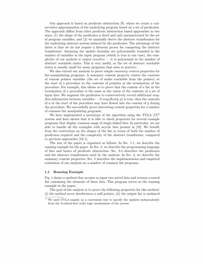
Fig. 1 shows a method that accepts as input two sorted lists and returns a sortedlist containing the elements of these lists. This program serves as the runningexample in the paper.

The goal of the analysis is to prove the following properties for this method:(i) the method never dereferences a null pointer, (ii) the output list is unshared

4 We used TVLA mainly as a convenient way to specify the updates independentlyfrom the 3-valued first order logic mechanisms of the system.

and acyclic, (iii) the method does not create a memory leak, and (iv) the set ofcells in the output list is the union of the sets of cells of the two input lists.

List Merge(List p, List q) {L0: if (p == null) return q;

L1: if (q == null) return p;

L2: if (p.data < q.data) { h = p; p = p.n; }L3: else { h = q; q = q.n; }L4: t = h;

L5: while (p != null && q != null) {L6: if (p.data < q.data) {L7: t.n = p;

L8: temp = p.n;

L9: p = temp;

}L10: else {L11: t.n = q;

L12: temp = q.n;

L13: q = temp;

}L14: t = t.n;

}L15: if (p != null) { t.n = p; }L16: else if (q != null) { t.n = q; }L17: return h;

}

Fig. 1. A C# method that merges two singly-linked list into one list

2 Background

In this section, we define a simple programming language for singly-linked lists,and the concrete semantics. We also describe the basics of predicate abstraction.

2.1 A Simple Programming Language of Singly-Linked Lists

Our language contains a single data type List (representing a singly-linked list)declared as

class List {List n; int data;}.The programming language conservatively ignores the data field of the list type.

Let PVar be a set of variables of type List . A program is a control flow graph(CFG), where each node in the CFG represents a control location and there isan entry node entry, and an exit node exit. The edges in the CFG representeither assignment statements, assume statements, or assert statements.

There are five types of assignment statements: (1) x := new List(), (2) x :=null, (3) x := y, (4) x := y.n, and (5) x.n := y. Control flow is achieved by usingthe assume statements. An assume statement is of the form assume (x == y)

or assume (x! = y), and an assert statement is of the form assert (x == y) orassert (x! = y).

We also assume that programs in this language are normalized in the follow-ing way. Every statement of the form x=y or x=y.n is preceded by a statementx=null; every statement of the form x.n=y is preceded by a statement of theform x.n=null; in every statement of the form y=x.n or x.n=y the variablesx and y are different. Finally, every statement that dereferences a variable x

is preceded by an assert statement assert (x! = null). These assumptions arenot restrictive, as it is possible to preprocess programs in linear time into thenormalized form by introducing new temporaries, however they do simplify thespecification of the abstract semantics shown later.

Semantics. A concrete state of the program σ is an evaluation of: (i) eachvariable x ∈ PVar as an object of type List , and (ii) the field n as a function nfrom List to List . We often refer to an object of type List as a (list) cell. Wedenote x as the value of a program variable x ∈ PVar in a given state. For anystate, we require that n(null) = null .

We associate a transition function [[st ]] with every statement st in the pro-gram. Each statement st takes a concrete state σ, and transforms it to a stateσ′ = [[st ]](σ). The concrete semantics of program statements is shown in Table 1.The semantics is insensitive to the possible existence of garbage cells (i.e., cellsthat are not reachable from any variable). This is achieved by restricting thethe variables that appear in all first-order formulae to range exclusively overnon-garbage cells. This restriction is implicitly used throughout this paper.

Table 1. Concrete semantics of program statements. Unprimed symbols denote valuesbefore a statement is executed and primed symbols denote post-execution values

Statement Semantics

x = new List() x′ = vnew,

n′ = λ v . (v = vnew ? null : n(v))where vnew is a fresh cell

x = null x′ = null

x = y x′ = y

x = y.n x′ = n(y)

x.n = null n′ = λ v . (v = x ? null : n(v))

x.n = y n′ = λ v . (v = x ? y : n(v))

assert(x != y) if x 6= y then nop else abort with error message

assert(x == y) if x = y then nop else abort with error message

assume(x != y) if x 6= y then nop else ignore execution

assume(x == y) if x = y then nop else ignore execution

2.2 Predicate Abstraction

Predicate abstraction [9] is a scheme for performing abstract interpretation [6] ofprograms. A predicate Pi is a Boolean expression over the signature Σ ∪ PVar,where Σ consists of a set of interpreted function or predicate symbols.

Given a set of predicates P = {P1 , . . . ,Pn}, predicate abstraction approxi-mates the concrete set of states by Boolean combinations of predicates in P . Anabstract state sa is an evaluation of the predicates in P to Boolean values {0, 1}.Alternately, we can view an abstract state as a conjunction

∧

Pi∈P P̃i, where

P̃i ⊆ {Pi,¬Pi}. Such a conjunction is called a cube over P . Given a concretestate σ, the abstraction operation α maps σ to an abstract state by evaluatingthe predicates on σ. The operation γ maps a abstract state to the set of concretestates it represents. We define α and γ for a set of states by pointwise extensionof the operations for individual elements.

Given a program and a set of predicates P , we can define an abstract tran-sition relation [[st ]]# for each statement st in the program as follows:

[[st ]]#(sa) = {α(ta) | ta ∈ [[st ]](γ(sa))} .

We also refer to the abstract transition relation as the best transformer.Predicate abstraction provides a conservative approximation of the underly-

ing concrete system — if we prove a property φ on the abstract program, thenthe property also holds for the underlying concrete program. However, a coun-terexample to φ in the abstract system need not be realizable in the concretesystem.

3 A Static Analysis for Acyclic Unshared Lists

In this section, we define a static analysis based on predicate abstraction forprograms in the language described in Sec. 2.1. We start by giving basic defini-tions needed to formally define acyclic unshared lists. We then describe a newpredicate abstraction for acyclic unshared lists and explain how to express dif-ferent properties over the predicates. Finally, we provide the abstract semanticsfor every program statement.

3.1 Definitions

In the sequel, we will use the notation nj to denote the jth application of thefunction n. The relation n∗ stands for the reflexive transitive closure of n, i.e.,n∗(u, v) is true if and only if there exists a j ≥ 0 such that nj(u) = v, and n+

stands for the non-reflexive transitive closure of n, i.e., n+(u, v) is true if andonly if there exists a j > 0 such that nj(u) = v.

Definition 1. We say that a heap is acyclic, when for every cell u of type List(apart from null), n+(u, u) is false.

Definition 2. We say that a heap is unshared, when for every pair of cells uand v (apart from null) of type List, n(u) = n(v) ⇔ (u = v ∨ n(u) = null).

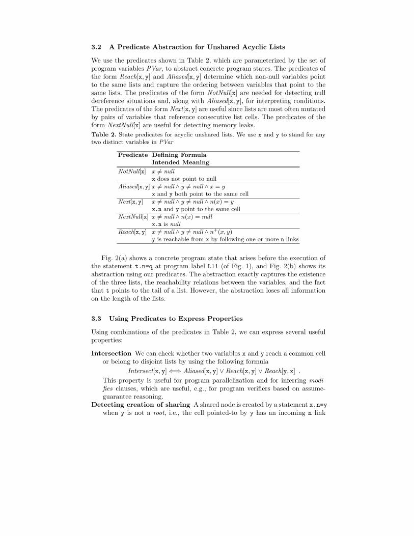
3.2 A Predicate Abstraction for Unshared Acyclic Lists

We use the predicates shown in Table 2, which are parameterized by the set ofprogram variables PVar, to abstract concrete program states. The predicates ofthe form Reach[x, y] and Aliased[x, y] determine which non-null variables pointto the same lists and capture the ordering between variables that point to thesame lists. The predicates of the form NotNull[x] are needed for detecting nulldereference situations and, along with Aliased[x, y], for interpreting conditions.The predicates of the form Next[x, y] are useful since lists are most often mutatedby pairs of variables that reference consecutive list cells. The predicates of theform NextNull[x] are useful for detecting memory leaks.

Table 2. State predicates for acyclic unshared lists. We use x and y to stand for anytwo distinct variables in PVar

Predicate Defining Formula

Intended Meaning

NotNull[x] x 6= nullx does not point to null

Aliased[x, y] x 6= null ∧ y 6= null ∧ x = y

x and y both point to the same cell

Next[x, y] x 6= null ∧ y 6= null ∧ n(x) = y

x.n and y point to the same cell

NextNull[x] x 6= null ∧ n(x) = nullx.n is null

Reach[x, y] x 6= null ∧ y 6= null ∧ n+(x, y)y is reachable from x by following one or more n links

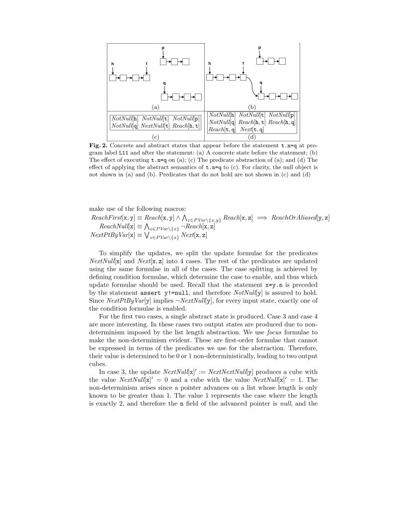
Fig. 2(a) shows a concrete program state that arises before the execution ofthe statement t.n=q at program label L11 (of Fig. 1), and Fig. 2(b) shows itsabstraction using our predicates. The abstraction exactly captures the existenceof the three lists, the reachability relations between the variables, and the factthat t points to the tail of a list. However, the abstraction loses all informationon the length of the lists.

3.3 Using Predicates to Express Properties

Using combinations of the predicates in Table 2, we can express several usefulproperties:

Intersection We can check whether two variables x and y reach a common cellor belong to disjoint lists by using the following formula

Intersect[x, y] ⇐⇒ Aliased[x, y] ∨ Reach[x, y] ∨ Reach[y, x] .

This property is useful for program parallelization and for inferring modi-fies clauses, which are useful, e.g., for program verifiers based on assume-guarantee reasoning.

Detecting creation of sharing A shared node is created by a statement x.n=ywhen y is not a root, i.e., the cell pointed-to by y has an incoming n link

from a non-garbage cell u. We define the macro

IsRoot[y] ≡∧

z∈PVar\{y}

¬Reach[z, y]

and check whether ¬IsRoot[y] holds to detect creation of sharing.

Detecting creation of cycles A cycle is created by a statement x.n=y whenthere exists a (possibly empty) path of n links from the cell pointed-to by y

to the cell pointed-to by x. We define the macro

ReachOrAliased[y, x] ≡ Aliased[y, x] ∨ Reach[y, x]

and check whether ReachOrAliased[y, x] holds to detect these situations.

Detecting memory leaks A memory leak can occur for two types of state-ments — x=null and x.n=null.

In the first case, a leak is created when x is not already null and it is thelast reference to a cell. We define the macro

LastRef[x] ≡ NotNull[x] ∧ IsRoot[x] ∧∧

w∈PVar\{x}

¬Aliased[x, w]

and whether LastRef[x] holds to detect a possible memory leak.

In the second case, a leak is created when x.n is not already null and it is thelast reference to a cell. Since we assume there is no sharing, the statementdoes not cause a memory leak if and only if x.n is referenced by anotherprogram variable. We define the macro

NextPtByVar[x] ≡∨

w∈PVar\{x}

Next[x, w]

and check whether ¬NextNull[x]∧¬NextPtByVar[x] holds to detect a possiblememory leak.

Detecting null dereferences To detect null dereferences and interpret pro-gram conditions, we define the macro

IsNull[x] ≡ ¬NotNull[x] .

3.4 An Abstract Semantics for Program Statements

Table 3 contains the update formulae for all program statements except x=y.n.For every predicate that is affected by the statement, the value in the next state(appearing on left side of :=) is computed by a Boolean combination of thepredicates in the current state (the right side of :=). To save space, we do notmention the predicates that are not affected by the statement. Notice that thesize of the update formulae in Table 3 is constant (at most 5 literals are used)and, therefore, the time to compute an output abstract state (a cube) is linearin the number of predicates. Also, the abstract semantics for these statementsproduces a single output state from every input state.

Fig. 3 shows the predicate update formulae for the program statement x=y.n,which are more complex than the updates for the other statements. The formulae

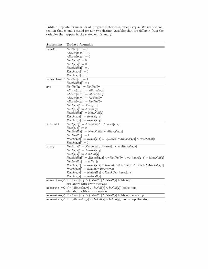
Table 3. Update formulae for all program statements, except x=y.n. We use the con-vention that w and z stand for any two distinct variables that are different from thevariables that appear in the statement (x and y)

Statement Update formulae

x=null NotNull[x]′ := 0Aliased[x, w]′ := 0Aliased[w, x]′ := 0Next[x, w]′ := 0Next[w, x]′ := 0NextNull[x]′ := 0Reach[x, w]′ := 0Reach[w, x]′ := 0

x=new List() NotNull[x]′ := 1NextNull[x]′ := 1

x=y NotNull[x]′ := NotNull[y]Aliased[x, z]′ := Aliased[y, z]Aliased[z, x]′ := Aliased[z, y]Aliased[x, y]′ := NotNull[y]Aliased[y, x]′ := NotNull[y]Next[x, z]′ := Next[y, z]Next[z, x]′ := Next[z, y]NextNull[x]′ := NextNull[y]Reach[x, z]′ := Reach[y, z]Reach[z, x]′ := Reach[z, y]

x.n=null Next[w, z]′ := Next[w, z] ∧ ¬Aliased[x, z]Next[x, z]′ := 0NextNull[z]′ := NextNull[z] ∨ Aliased[z, x]NextNull[x]′ := 1Reach[w, z]′ := Reach[w, z] ∧ ¬(ReachOrAliased[w, x] ∧ Reach[x, z])Reach[x, z]′ := 0

x.n=y Next[w, z]′ := Next[w, z] ∨ Aliased[w, x] ∧ Aliased[z, y]Next[x, z]′ := Aliased[z, y]Next[x, y]′ := NotNull[y]NextNull[z]′ := Aliased[z, x] ∧ ¬NotNull[y] ∨ ¬Aliased[z, x] ∧ NextNull[z]NextNull[x]′ := IsNull[y]Reach[w, z]′ := Reach[w, z] ∨ ReachOrAliased[w, x] ∧ ReachOrAliased[y, z]Reach[x, z]′ := ReachOrAliased[y, z]Reach[w, y]′ := NotNull[y] ∧ ReachOrAliased[w, x]Reach[x, y]′ := NotNull[y]

assert(x==y) if Aliased[x, y] ∨ (IsNull[x] ∧ IsNull[y] holds nopelse abort with error message

assert(x!=y) if ¬(Aliased[x, y] ∨ (IsNull[x] ∧ IsNull[y]) holds nopelse abort with error message

assume(x==y) if Aliased[x, y] ∨ (IsNull[x] ∧ IsNull[y] holds nop else stop

assume(x!=y) if ¬(Aliased[x, y] ∨ (IsNull[x] ∧ IsNull[y]) holds nop else stop

th

q

p

th

q

p

(a) (b)

NotNull[h] NotNull[t] NotNull[p]NotNull[q] NextNull[t] Reach[h, t]

NotNull[h] NotNull[t] NotNull[p]NotNull[q] Reach[h, t] Reach[h, q]Reach[t, q] Next[t, q]

(c) (d)

Fig. 2. Concrete and abstract states that appear before the statement t.n=q at pro-gram label L11 and after the statement: (a) A concrete state before the statement; (b)The effect of executing t.n=q on (a); (c) The predicate abstraction of (a); and (d) Theeffect of applying the abstract semantics of t.n=q to (c). For clarity, the null object isnot shown in (a) and (b). Predicates that do not hold are not shown in (c) and (d)

make use of the following macros:

ReachFirst[x, y] ≡ Reach[x, y] ∧ ∧

z∈PVar\{x,y} Reach[x, z] =⇒ ReachOrAliased[y, z]

ReachNull[x] ≡ ∧

z∈PVar\{x} ¬Reach[x, z]

NextPtByVar[x] ≡ ∨

z∈PVar\{x} Next[x, z]

To simplify the updates, we split the update formulae for the predicatesNextNull[x] and Next[x, z] into 4 cases. The rest of the predicates are updatedusing the same formulae in all of the cases. The case splitting is achieved bydefining condition formulae, which determine the case to enable, and thus whichupdate formulae should be used. Recall that the statement x=y.n is precededby the statement assert y!=null, and therefore NotNull[y] is assured to hold.Since NextPtByVar[y] implies ¬NextNull[y], for every input state, exactly one ofthe condition formulae is enabled.

For the first two cases, a single abstract state is produced. Case 3 and case 4are more interesting. In these cases two output states are produced due to non-determinism imposed by the list length abstraction. We use focus formulae tomake the non-determinism evident. These are first-order formulae that cannotbe expressed in terms of the predicates we use for the abstraction. Therefore,their value is determined to be 0 or 1 non-deterministically, leading to two outputcubes.

In case 3, the update NextNull[x]′ := NextNextNull[y] produces a cube withthe value NextNull[x]′ = 0 and a cube with the value NextNull[x]′ = 1. Thenon-determinism arises since a pointer advances on a list whose length is onlyknown to be greater than 1. The value 1 represents the case where the lengthis exactly 2, and therefore the n field of the advanced pointer is null, and the

value 0 represents the cases where the length is greater than 2 and therefore then field of the advanced pointer is not null.

In case 4, the update Next[x, z]′ := NextNextPtByVar[y] ∧ ReachFirst[y, z]produces an abstract state with the value Next[x, z]′ := ReachFirst[y, z] andan abstract state with the value Next[x, z]′ := 0. The non-determinism arisessince a pointer advances into a list that reaches another pointer variable, sayz, which is the closest among the variables following y. However, the lengthof the path between y and z is only known to be greater than 1. The value0 represents the case where the length is greater than 2, and therefore the n

field of the advanced pointer is not pointed-to by any variable, and the valueReachFirst[y, z] represents the case where the length is exactly 2 and thereforethe n field of the advanced pointer is pointed-to by z.

Case 2 and case 4 contain predicate update formulae that are linear in thenumber of variables (for the predicates of the form Next[x, z] and NextNull[x]).Therefore, the time to produce an output state from an input state is states isO(n

√n) where n is the number of predicates (and n = O(k2) where k is the

number of program variables).The size of the update formulae for all program statements are at most

quadratic in the number of variables. This means that the time to produce anew abstract state from an existing abstract state is polynomial in the numberof predicates. Therefore, the analysis has polynomial output sensitivity, i.e., theanalysis time is polynomial in the number of reachable abstract states.

Fig. 2(d) shows the effect of applying the update formulae for t.n=q to theabstract state in Fig. 2(c). The output state precisely captures the reachabilitybetween all program variables and the fact that t and q point to adjacent cells.

We claim that the update formulae above provide the best transformers forthe respective program statements. In Appendix B, we provide a methodologyfor deriving optimal abstract transformers for program statements. In particular,we prove that the abstract transformers for all statements except x=y.n arecomplete, and that the abstract transformer for x=y.n is the best transformer.

4 Summary Content Properties

In this section, we extend our analysis for linked lists to prove a set of moreinteresting properties, we call summary content properties. Intuitively, our goalis to relate the content5 of the lists, at any control location l1 in the program,with the content of the lists at the control location entry in the program. This isan extension of the memory leak property, where we also check that the contentof certain lists only end up in certain other lists. This is particularly useful forproving the relationships of the contents between the lists that are passed asinput to a procedure and the lists that are returned from the procedure. Forexample, one can show that after reversing a list, the content of the output listis exactly the content of the input list.

5 We use content to refer to all the cells reachable from a pointer variable, and notthe value inside the cells.

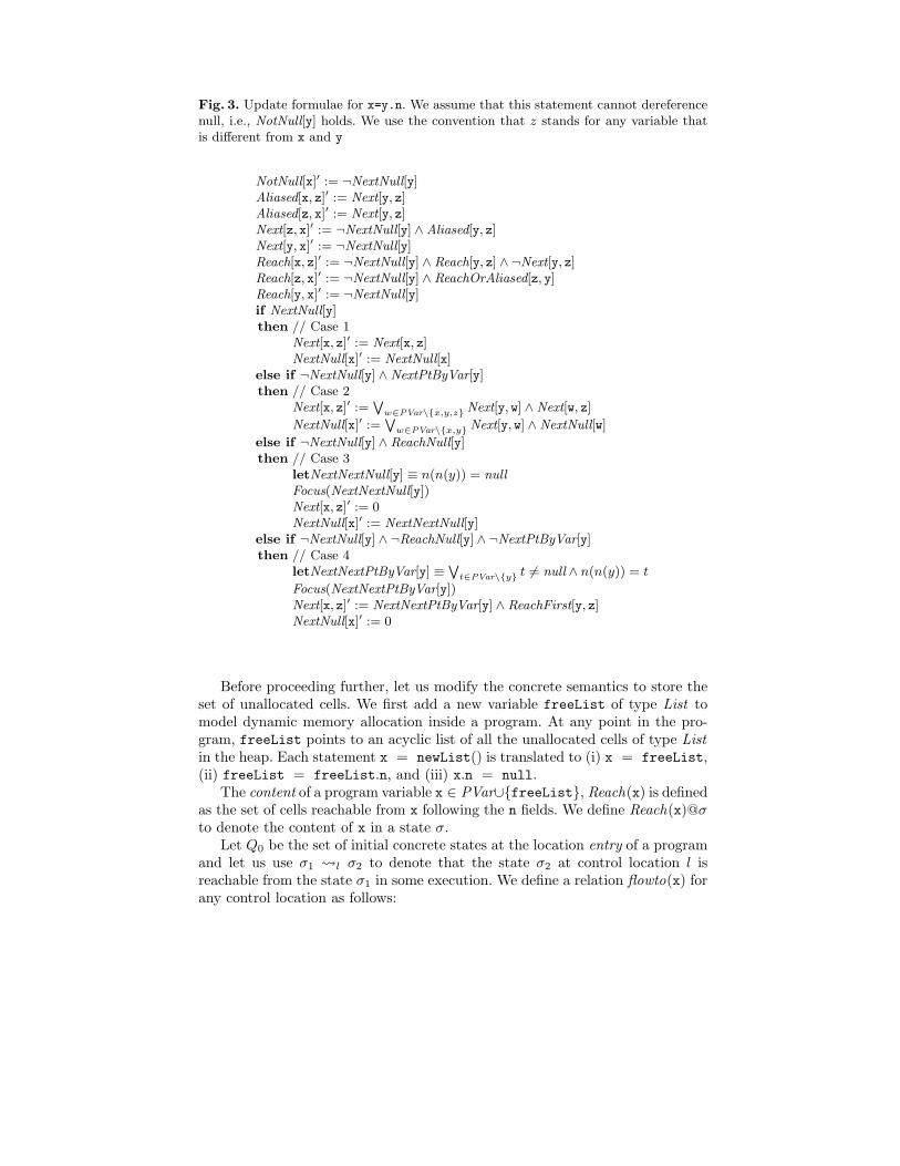
Fig. 3. Update formulae for x=y.n. We assume that this statement cannot dereferencenull, i.e., NotNull[y] holds. We use the convention that z stands for any variable thatis different from x and y

NotNull[x]′ := ¬NextNull[y]Aliased[x, z]′ := Next[y, z]Aliased[z, x]′ := Next[y, z]Next[z, x]′ := ¬NextNull[y] ∧ Aliased[y, z]Next[y, x]′ := ¬NextNull[y]Reach[x, z]′ := ¬NextNull[y] ∧ Reach[y, z] ∧ ¬Next[y, z]Reach[z, x]′ := ¬NextNull[y] ∧ ReachOrAliased[z, y]Reach[y, x]′ := ¬NextNull[y]if NextNull[y]then // Case 1

Next[x, z]′ := Next[x, z]NextNull[x]′ := NextNull[x]

else if ¬NextNull[y] ∧ NextPtByVar[y]then // Case 2

Next[x, z]′ :=W

w∈PVar\{x,y,z} Next[y, w] ∧ Next[w, z]

NextNull[x]′ :=W

w∈PVar\{x,y} Next[y, w] ∧ NextNull[w]

else if ¬NextNull[y] ∧ ReachNull[y]then // Case 3

letNextNextNull[y] ≡ n(n(y)) = nullFocus(NextNextNull[y])Next[x, z]′ := 0NextNull[x]′ := NextNextNull[y]

else if ¬NextNull[y] ∧ ¬ReachNull[y] ∧ ¬NextPtByVar[y]then // Case 4

letNextNextPtByVar[y] ≡W

t∈PVar\{y} t 6= null ∧ n(n(y)) = t

Focus(NextNextPtByVar[y])Next[x, z]′ := NextNextPtByVar[y] ∧ ReachFirst[y, z]NextNull[x]′ := 0

Before proceeding further, let us modify the concrete semantics to store theset of unallocated cells. We first add a new variable freeList of type List tomodel dynamic memory allocation inside a program. At any point in the pro-gram, freeList points to an acyclic list of all the unallocated cells of type Listin the heap. Each statement x = newList() is translated to (i) x = freeList,(ii) freeList = freeList.n, and (iii) x.n = null.

The content of a program variable x ∈ PVar∪{freeList}, Reach(x) is definedas the set of cells reachable from x following the n fields. We define Reach(x)@σto denote the content of x in a state σ.

Let Q0 be the set of initial concrete states at the location entry of a programand let us use σ1 l σ2 to denote that the state σ2 at control location l isreachable from the state σ1 in some execution. We define a relation flowto(x) forany control location as follows:

Definition 3. For any control location l, and for any variable x ∈ PVar ∪{freeList}, we define flowto(x) at l as {y ∈ PVar | ∃σ0 ∈ Q0,∃σ,σ0 l

σ,Reach(x)@σ0 ∩ Reach(y)@σ 6= {}}The definition basically says that flowto(x) at any control location is the set

of variables whose reachable set intersects with the content of x in some initialstate. In other words, these are the variables that the content of x in Q0 haveflown into. We extend both Reach, and flowto(·) to operate on a set of programvariables, by simply taking pointwise union over the set.

To capture the flowto() information conservatively, we maintain a predicatemayflow(x) for each variable x in the abstract state. For any program location l,flowto(x) ⊆ mayflow(x). In other words, mayflow() maintains flowto() informa-tion conservatively. In the next section, we provide the updates to this predicateand show that the updates are conservative.

4.1 Updating mayflow

In any state σ0 ∈ Q0, we initialize mayflow() as follows:

mayflow(x) = {y ∈ PVar | Intersect[y, x]}The content of x in σ0 intersects with the content of all the variables t thatsatisfies Intersect[t, x]. Notice that the mayflow sets can be empty for variablesthat point to null.

Let us look at the different statements:

1. x = null: For every z ∈ PVar,

mayflow(z)′ = mayflow(z) \ {x}After x is assigned null, the content of x (the set {}) can’t intersect withthe content of any variable. Hence we remove x from the mayflow() of everyvariable z.

2. x = new List(): Assuming this statement is preceded by x = null, weonly update mayflow(freeList):

mayflow(freeList)′ = mayflow(freeList) ∪ {x}After this statement, x holds a cell initially reachable from freeList in σ0.

3. x = y: We know that x is null before this statement. For any variable z

such that y ∈ mayflow(z):

mayflow(z)′ = mayflow(z) ∪ {x}4. x = y.n: We know that x is null before this statement. For any variable z

such that y ∈ mayflow(z):

mayflow(z)′ = mayflow(z) ∪ {x}5. x.n = y: We know that x.n is null before this statement. For any variable

z such that y ∈ mayflow(z):

mayflow(z)′ = mayflow(z) ∪ {w | ReachOrAliased[w, x]}After this statement, every variable that reaches x could intersect with theinitial content of all z that y (potentially) intersects before the statement.

6. x.n = null: In this case, the mayflow() relation does not change.

The updates ensure that mayflow() overapproximates the flowto() set at eachprogram location.

4.2 Proving Summary Content Properties

We now define a summary content property to relate the contents of two sets ofvariables VI and VO in the program as follows:

Definition 4. For two sets of variables VI ⊆ PVar and VO ⊆ PVar, we definea summary content property SC (VI ,VO) to denote that for any state σ0 ∈ Q0,and a state σ at location l such σ0 l σ, Reach(VO)@σ = Reach(VI )@σ0 .

The following proposition allows us to prove such summary content propertiesusing the existing predicates augmented with mayflow() predicates:

Proposition 1. For any program manipulating acyclic unshared lists, and twosets of variables VI ⊆ PVar and VO ⊆ PVar, and any abstract state sa such that:

1. The program has no memory leaks for every possible reachable state,2. For every y ∈ mayflow(VI ) in sa, either y ∈ VO or y = null in sa or there

exists a z ∈ VO such that ReachOrAliased[z, y] in sa, and3. For every y ∈ VO in sa, such that y ∈ mayflow(z) in sa but z 6∈ VI , either

z = null at α(Q0) or there exists a variable x ∈ VI and ReachOrAliased[x, z]at α(Q0).

Then, SC (VI ,VO) in all the concrete states represented by sa.

We note that Proposition 1 can be expressed as a Boolean formula overthe predicates in a given abstract state. Hence, the property can be checkedautomatically. The above proposition enables us to relate the contents of thevariables in VO at the control location exit in the program with the contentsof the variables in VI at the entry to the program, after the abstract analysisterminates.

We also note that the requirement for absence of memory leaks can be liftedand the analysis can be extended to handle memory deallocation statements.However, we do not discuss the details of these extensions here.

4.3 Example

Let us consider the merge example from Figure 1. Let us consider the case whenboth p and q are not null. The summary content property of interest in this caseis SC ({p, q}, {h}) at the location L17, i.e., we want to check that the content ofthe output list (pointed to-by h) is precisely the union of content of the disjointlists pointed-to by p and q.

Since all the variables apart from p and q are local, they are initialized to null.Hence the initial content of all the local variables is {}, and hence mayflow(x)for any local variable x remains {} throughout.

The assignments in L2 and L3 results in mayflow(p) = {p, h} and mayflow(q) ={q, h}. After L4, mayflow(p) = {p, h, t} and mayflow(q) = {q, h, t}. After ex-ecuting L7, the mayflow information remains unchanged. Also note that theprogram obtained after preprocessing the example in Figure 1 assigns null totemp before L8; hence temp does not belong to mayflow(p) and mayflow(q).Hence, after executing L8 and L9, mayflow(p) = {p, h, t, temp}, but does notcontain q.

Finally, one can verify that at L17, mayflow(p) = {p, h, t, temp}, and mayflow(q) ={q, h, t, temp}. But, we know that at this point ReachOrAliased[h, t], and either(i) both p and q are null or (ii) p is null and ReachOrAliased[h, q] or (iii) q is nulland ReachOrAliased[h, p]. Also, either temp is null or ReachOrAliased[h, temp]holds. Moreover, our analysis also proves that there is no memory leak in theprogram. Therefore, by Proposition 1, we can conclude that SC ({p, q}, {h})holds at exit.

5 Experimental Results

We used TVLA to implement our analysis based on the predicates and abstracttransformers described in Sec. 3. We applied the analysis to verify various speci-fications of programs operating on lists, described in Table 4. The table contains,in each column the measures produced by the analysis in this paper (left side)to the measures produced by the analysis in [19] (right side). (We have not runthe analysis of [19] on the append and append nullderef examples.) For allexamples, in addition to checking that lists do not become cyclic or shared, wechecked the absence of null dereferences and absence of memory leaks.

The merge and bubbleSort examples create temporary sharing patterns. Ouranalysis detects these cases and provides the information needed to understandwhich statements are responsible for creating the sharing. We modified theseexamples by changing the order in which the n links are mutated and thusavoided created temporary sharing. In the bubbleSort example, three variablespoint to three adjacent cells and are used to swap the order of the second andthird cells. Avoiding sharing consists of first setting the n links of the three cells,and then setting the links to reflect the new order between the cells.

The experiments were conducted using TVLA version 2, running with SUN’sJRE 1.5, on a desktop computer with a 3.4 GHZ Intel Pentium Processor with1 GB RAM. The results of the analysis are shown in Table 4. In all of theexamples, the analysis produced no false alarms. For the search nullderef

and append nullderef the analysis detected the null dereference violations.Although the examples we have used are rather small (at most 40 CFG lo-

cations and 67 CFG edges), we are encouraged by the low running times ofthe analysis. It is also interesting that our analysis was able to prove the sameproperties as the analysis in [19] using less time and space resources and fewerreachable states (indicated by the #Cubes column). Although it is hard to pre-dict whether the analysis will be faster for larger examples from the times takenon the current examples, we believe that the reduction of the number of reach-able states (ranging between 1.8 and 4.9) is an indication that the analysis in

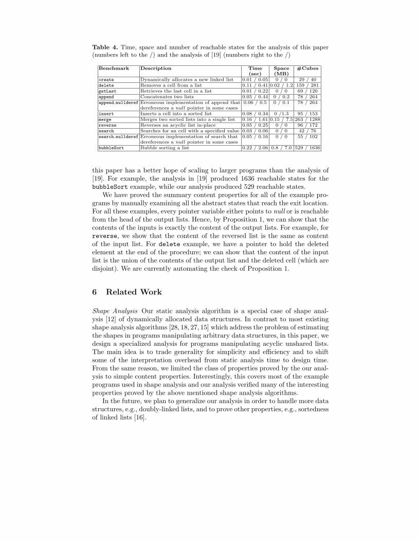
Table 4. Time, space and number of reachable states for the analysis of this paper(numbers left to the /) and the analysis of [19] (numbers right to the /)

Benchmark Description Time Space #Cubes(sec) (MB)

create Dynamically allocates a new linked list 0.01 / 0.05 0 / 0 29 / 40delete Removes a cell from a list 0.11 / 0.41 0.02 / 1.2 159 / 281getLast Retrieves the last cell in a list 0.01 / 0.22 0 / 0 69 / 120append Concatenates two lists 0.05 / 0.44 0 / 0.2 78 / 264append nullderef Erroneous implementation of append that 0.06 / 0.5 0 / 0.1 78 / 264

dereferences a null pointer in some casesinsert Inserts a cell into a sorted list 0.08 / 0.34 0 /1.3 95 / 153merge Merges two sorted lists into a single list 0.16 / 1.61 0.15 / 7.5 263 / 1288reverse Reverses an acyclic list in-place 0.05 / 0.25 0 / 0 96 / 172search Searches for an cell with a specified value 0.03 / 0.06 0 / 0 42 / 76search nullderef Erroneous implementation of search that 0.05 / 0.16 0 / 0 55 / 102

dereferences a null pointer in some casesbubbleSort Bubble sorting a list 0.22 / 2.06 0.8 / 7.0 529 / 1636

this paper has a better hope of scaling to larger programs than the analysis of[19]. For example, the analysis in [19] produced 1636 reachable states for thebubbleSort example, while our analysis produced 529 reachable states.

We have proved the summary content properties for all of the example pro-grams by manually examining all the abstract states that reach the exit location.For all these examples, every pointer variable either points to null or is reachablefrom the head of the output lists. Hence, by Proposition 1, we can show that thecontents of the inputs is exactly the content of the output lists. For example, forreverse, we show that the content of the reversed list is the same as contentof the input list. For delete example, we have a pointer to hold the deletedelement at the end of the procedure; we can show that the content of the inputlist is the union of the contents of the output list and the deleted cell (which aredisjoint). We are currently automating the check of Proposition 1.

6 Related Work

Shape Analysis Our static analysis algorithm is a special case of shape anal-ysis [12] of dynamically allocated data structures. In contrast to most existingshape analysis algorithms [28, 18, 27, 15] which address the problem of estimatingthe shapes in programs manipulating arbitrary data structures, in this paper, wedesign a specialized analysis for programs manipulating acyclic unshared lists.The main idea is to trade generality for simplicity and efficiency and to shiftsome of the interpretation overhead from static analysis time to design time.From the same reason, we limited the class of properties proved by the our anal-ysis to simple content properties. Interestingly, this covers most of the exampleprograms used in shape analysis and our analysis verified many of the interestingproperties proved by the above mentioned shape analysis algorithms.

In the future, we plan to generalize our analysis in order to handle more datastructures, e.g., doubly-linked lists, and to prove other properties, e.g., sortednessof linked lists [16].

Decision Procedures In a seminal paper in 1969, Rabin showed the monadic sec-ond order logic with one function symbol is decidable [22]. This allows to mod-ularly verify programs manipulating singly linked lists. Indeed, the Mona sys-tem automatically proves partial correctness of programs manipulating unsharedacyclic lists and trees assuming programmer specified pre- and post-conditions,and loop invariants expressed in Monadic second order logic [21].

Decision procedures can be also employed to automatically generate the besttransformers in abstract interpretation and thus avoid the need for programmerspecified loop invariants [24]. In this paper we focused on a specific parametricabstraction and eliminated the need for employing decision procedures at anal-ysis time. For example, the analysis of bubble-sort takes 0.22 seconds by ouranalysis in contrast to 204 seconds (5, 930 calls to a theorem prover) in [2] whichuses a specialized decision procedure. Of course, decision procedures can stillbe employed at analysis generation time to automate the design of specializedshape analyses.

Shape Analysis via Predicate Abstraction Predicate abstraction was used forshape analysis in [7, 1, 19]. The present paper provides an effective solution tothe limited problem of proving content properties of unshared acyclic linked lists.

Regular Model Checking Recently regular model checking was also employed toprove properties of programs manipulating singly linked lists [4, 3]. The cost oftheir analysis is comparable with the cost of decision procedures and is up tothree orders of magnitude slower than our analysis.

Separation Logic Separation logic [11] allows to separate assertions on the heapinto claims about disjoints parts the heap. This goes beyond our method whichonly separates the treatments of disjoint lists. For example, when a part of a listis mutated, our analysis can change the predicates of the whole list. In the futurewe plan to use the notion of cutpoints [25, 26] in order to handle procedures bylocalizing the treatment of procedure calls.

References

1. I. Balaban, A. Pnueli, and L. D. Zuck. Shape analysis by predicate abstrac-tion. In Radhia Cousot, editor, Proceedings of the 6th International Conferenceon Verification, Model Checking and Abstract Interpretation, VMCAI 2005, vol-ume 3148 of Lecture Notes in Computer Science. Springer, January. Available athttp://www.cs.tau.ac.il/∼rumster/vmcai05.pdf.

2. J. Bingham and Z. Rakamaric. A logic and decision procedure for predicate ab-straction of heap-manipulating programs. Technical report, Intel Corp., 2005.http://www.cs.ubc.ca/cgi-bin/tr/2005/TR-2005-19.pdf.

3. A. Bouajjani, P. Habermehl, P. Moro, and T. Vojnar. Verifying programs withdynamic 1-selector-linked structures in regular model checking. In In Proc. 12thIntern. Conf. on Tools and Algorithms for the Construction and Analysis of Sys-tems (TACAS’05), volume 3440 of LNCS, April 2005.

4. A. Bouajjani, P. Habermehl, and T. Vojnar. Abstract regular model checking.In In Proc. 16th Intern. Conf. on Computer Aided Verification (CAV’04), LNCS,July 2004.

5. V. T. Chakaravarthy. New results on the computability and complexity of points–to analysis. In Proceedings of the 30th ACM SIGPLAN-SIGACT symposium onPrinciples of programming languages, pages 115–125. ACM Press, 2003.

6. P. Cousot and R. Cousot. Abstract interpretation: a unified lattice model for staticanalysis of programs by construction or approximation of fixpoints. In ConferenceRecord of the Fourth Annual ACM SIGPLAN-SIGACT Symposium on Principlesof Programming Languages, pages 238–252, Los Angeles, California, 1977. ACMPress, New York, NY.

7. D. Dams and K. S. Namjoshi. Shape analysis through predicate abstraction andmodel checking. In Proceedings of the 4th International Conference on Verification,Model Checking, and Abstract Interpretation, pages 310–324. Springer-Verlag, 2003.

8. G. Dong and J. Su. Incremental and decremental evaluation of transitive closureby first-order queries. Inf. Comput., 120(1):101–106, 1995.

9. S. Graf and H. Saidi. Construction of abstract state graphs with PVS. LNCS,1254:72–83, 1997.

10. N. Immerman. Descriptive Complexity. Springer-Verlag New York, Inc., 1994.11. S. S. Ishtiaq and P. W. O’Hearn. BI as an assertion language for mutable data

structures. ACM SIGPLAN Notices, 36(3):14–26, March 2001.12. N.D. Jones and S.S. Muchnick. Flow analysis and optimization of Lisp-like struc-

tures. In S.S. Muchnick and N.D. Jones, editors, Program Flow Analysis: Theoryand Applications, chapter 4, pages 102–131. Prentice-Hall, Englewood Cliffs, NJ,1981.

13. S. Lahiri and S. Qadeer. Verifying properties of well-founded linked lists. TechnicalReport MSR-TR-2005-97, Microsoft Research, July 2005.

14. W. Landi. Undecidability of static analysis. ACM Lett. Program. Lang. Syst.,1(4):323–337, 1992.

15. O. Lee, H. Yang, and K. Yi. Automatic verification of pointer programs usinggrammar-based shape analysis. In Sagiv, editor, Programming Languages and Sys-tems: 14th European Symposium on Programming, ESOP 2005, 2005.

16. T. Lev-Ami, T. Reps, M. Sagiv, and R. Wilhelm. Putting static analysis to workfor verification: A case study. In Proc. of the Int. Symp. on Software Testing andAnalysis, pages 26–38, 2000.

17. T. Lev-Ami and M. Sagiv. TVLA: A framework for Kleene based static analysis.In Proc. Static Analysis Symp., volume 1824 of LNCS, pages 280–301. Springer-Verlag, 2000.

18. T. Lev-Ami and M. Sagiv. TVLA: A system for implementing static analyses. InProc. Static Analysis Symp., pages 280–301, 2000.

19. R. Manevich, E. Yahav, G. Ramalingam, and M. Sagiv. Predicate abstraction andcanonical abstraction for singly-linked lists. In Radhia Cousot, editor, Proceedingsof the 6th International Conference on Verification, Model Checking and AbstractInterpretation, VMCAI 2005, volume 3148 of Lecture Notes in Computer Science.Springer, January. Available at http://www.cs.tau.ac.il/∼rumster/vmcai05.pdf.

20. Y. Matijasevic̆. Hilbert’s 10th Problem. MIT Press, 1993.21. A. Møller and M.I. Schwartzbach. The pointer assertion logic engine. In Proc.

ACM SIGPLAN Conference on Programming Language Design and Implementa-tion, PLDI ’01, June 2001. Also in SIGPLAN Notices 36(5) (May 2001).

22. M. Rabin. Decidability of second-order theories and automata on infinite trees.Trans. Amer. Math. Soc, 141(1):1–35, 1969.

23. G. Ramalingam. The undecidability of aliasing. ACM Transactions on Program-ming Languages and Systems, 16(5):1467–1471, 1994.

24. T. Reps, M. Sagiv, and G. Yorsh. Symbolic implementation of the best transformer.In Proc. Verification, Model Checking, and Abstract Interpretation, pages 252–266.Springer-Verlag, 2004.

25. N. Rinetzky, J. Bauer, T. Reps, M. Sagiv, and R. Wilhelm. A semantics forprocedure local heaps and its abstractions. In 32nd Annual ACM SIGPLAN-SIGACT Symposium on Principles of Programming Languages (POPL’05), 2005.

26. N. Rinetzky, M. Sagiv, and E. Yahav. Interprocedural shape analysis for cutpoint-free programs. In 12th International Static Analysis Symposium (SAS), 2005.

27. M. Sagiv, T. Reps, and R. Wilhelm. Parametric shape analysis via 3-valued logic.ACM Transactions on Programming Languages and Systems, 2002.

28. E. Y.-B. Wang. Analysis of Recursive Types in an Imperative Language. PhDthesis, Univ. of Calif., Berkeley, CA, 1994.

A Undecidability Results for Singly-linked Lists

In this section we strengthen Chakaravathy’s [5] undecidability result for theflow-sensitive may-aliasing problem on programs with singly-linked lists. Westart by explaining the setting for the original proof and repeating the originalproof. Then, we show how the proof can be modified to show undecidabilityunder more restricted semantics, thus strengthening this undecidability result.

A.1 Undecidability of Flow-Sensitive Analysiswith Singly-linked Lists

The problem of single-procedural flow-sensitive may-alias analysis of singly-linked lists is the following. Given the programming language described in Sec. 2,we define the all paths semantics to be the semantics that conservatively ignoresconditions. That is, the original conditions are replaced by if(..)then...else..., andwhile(..)... thus making every program path executable. Now, given two variablesp and q, the goal is to check if there is some path from the entry node to the exitnode in the control flow graph, such that, at the end of executing the statementsalong the path, p and q point to the same list cell.

Theorem 1 (Theorem 2 of [5]). Single-procedural flow-sensitive may-aliasanalysis of singly-linked lists is undecidable.

Proof. The problem of checking whether a multivariate polynomial has integerroots is known to be undecidable. In this problem, we are given a polynomialP (x1, x2, . . . , xn) over the variables x1, x2, . . . , xn. A sequence of (positive ornegative) integer constants a1, a2, . . . , an, not all zero, is called an integer rootof P if P (a1, a2, . . . , an) = 0. Given the polynomial, the problem is to check if ithas any integer roots. The problem is also known as the Hilberts tenth problem.Building on the work of Davis, Putnam and Robinson, Matijasevic̆ proved theundecidability of the Hilberts tenth problem [20].

We prove the undecidability result via a reduction from the above problem.The polynomial P (x1, x2, x3) = x1+x1x2−x2x3 is used as a running example to

illustrate the reduction. The output program for this example is given in the end.Here we explain the ideas used. The output program starts with the followingpiece of code:

Success = new List();Failure = new List();dummy = new List();D = new List();D.n = Success;Zero = temp = new List();While(..) { temp.n = new List(); temp = temp.n; }

The fifth statement makes D.n point to Success. We will make sure that thepolynomial has integer roots if and only if there is an execution path in whichD.n remains pointing to Success at the exit statement of the program. Thiswould prove the required undecidability. The next few statements in the abovecode create a singly linked list with Zero as the head. This would simulate thepositive integer number line, with the kth node representing integer k.

The next segment of the output program simulates choosing constant valuesfor each variable xi. The value has a magnitude and a (positive or negative) sign.To choose the magnitude of xi we use a pointer Xi and traverse the linked list.For our example polynomial, the next segment of code is:

X1 = Zero; While(..) {X1 = X1.n; }X2 = Zero; While(..) {X2 = X2.n; }X3 = Zero; While(..) {X3 = X3.n; }

If a path iterates the first loop a1 times,X1 would point to the ath1 node in our

linked list. This corresponds to assigning x1 = a1. In general, let X1,X2, . . . ,Xn

point to nodes a1, a2, . . . , an of the linked list. Then, this simulates choosingthese values for the variables.

Recall that we want to check if there is a non-zero integer root. Thus, weneed to ensure that at least one variable is assigned a non-zero value. The nextsegment of output our program, ensures that by using a multiway branch withn branches. The code segment for our example would be:

Switch(..) {Case: X1 = X1.n;Case: X2 = X2.n;Case: X3 = X3.n;

}As one of the branches must be executed, not all variables can point to node

zero of the linked list.Next we simulate choosing signs for the variables. As each of the n variables

can be positive or negative, the signs can be chosen in 2n possible ways. Weuse a multiway branch6 (a “switch” statement) with 2n branches to do the

6 The multiway branch can easily be translated into a sequence of if(..)then...else...statements.

simulation. Each branch represents choosing a particular combination of signsfor the variables. Consider any one branch with one such fixed combination ofsigns. Then the sign of any term in the polynomial also gets fixed. The sign ofa term is determined by its sign in the input polynomial and the combinationfixed by the branch. In our example, consider the branch that fixes x1, x3 to bepositive and x2 to be negative. Then, sign of the term −x2x3 would be positive.We separate the terms of the polynomial into groups of positive and negativeterms and get two polynomials P1 and P2. Then, a1, a2, . . . , an is an integerroot of P iff if P1(a1, a2, . . . , an) = P2(a1, a2, . . . , an). In our example, considera branch that represents choosing x1, x3 to be positive and x2 to be negative.Now, irrespective of the magnitudes, the terms x1 and −x2x3 would be positive,whereas the term x1x2 would be negative. So P1 = x1 + x2x3 and P2 = x1x2.

Before proceeding further, we define a macro7 used in the remainder of ourprogram. The macro takes two parameters A and B and checks if they point tothe same location:

ALIAS-CHECK(A,B) :temp1 = A.n;temp2 = B.n;A.n = D;B.n = dummy;A.n.n = Failure;A.n = temp1;B.n = temp2

Ignore the first two and the last two statements for the moment. Then, if Aand B point to different locations then the variable D would point to Failure.On the the other hand, if they point to the same location then D would remainpointing to Success and only a dummy variable will be made to point to Failure.The first two and the last two statements ensure that no other variable is affectedby this macro.

Recall that we want to check if the polynomials P1 and P2 evaluate to thesame value. For this purpose, we use two pointers p1 and p2. We first set p1 andp2 to point to node Zero of the linked list. Then we consider the terms of thepolynomial one by one. A term would contribute to P1 if it is positive and toP2 if it is negative. The sign of the term is determined by two factors: the signgiven to the term in the polynomial and which branch of the Switch statementwe are dealing with. Suppose the term contributes to P1. In that case we wouldmove p1 forward on the linked list. If it contributes to P2, we would move thepointer p2. In either case, the number of nodes by which the pointer moves isdetermined by the chosen values a1, a2, . . . , an. For example, let us take the termx1x2. Suppose we are writing code for the branch that represents choosing x1

and x3 to be positive and x2 to be negative. The term x1x2 would be negative.So, we move p2. We need to move it by a1 × a2 number of nodes. We use nestedloops to achieve this:

7 Using macros is not an issue, as they can always be expanded.

r1 = Zero;While(..) {

r1 = r1.n; r2 = Zero;While(..) { r2 = r2.n; p2 = p2.n; }

}

The problem with the above code is that the loops may be executed arbitrarynumber times. But we want the inner loop to run for exactly a2 iterations andthe outer loop for exactly a1 times. To ensure this, we use the fact that X1 andX2 are pointing to a1 and a2 and do alias checks. The new program fragment is:

r1 = Zero;While(..) {

r1 = r1.n;r2 = Zero;While(..) { r2 = r2.n; p2 = p2.n; }ALIAS-CHECK(X2, r2);

}ALIAS-CHECK(X1, r1);

Now either p2 points to node numbered a1 × a2 or D points to Failure. Ourprogram will make sure that it never goes back to Success. After evaluating allthe terms of the polynomial we finally check whether p1 and p2 point to thesame location, using the macro ALIAS-CHECK. Thus D can point to Successat the exit of the program iff the polynomial has integer roots.

For each term of the polynomial, we define a macro. The macro takes aparameter p. Suppose the the value of the term at the chosen constants is v,Then the macro either moves forward p by v nodes on the linked list or makesD point to Failure.

TERM1(p):r1 = Zero;While(..) {r1 = r1.n; p = p.n; }ALIAS-CHECK(X1, r1);

TERM2(p):r1 = Zero;While(..) {

r1 = r1.n;r2 = Zero;While(..) {r2 = r2.n; p = p.n; }ALIAS-CHECK(X2, r2);

}ALIAS-CHECK(X1, r1);

TERM3(p):r1 = Zero;

While(..) {r1 = r1.n;r3 = Zero;While(..) {r3 = r3.n; p = p.n; }ALIAS-CHECK(X3, r3);

}ALIAS-CHECK(X1, r1);

Now we are ready to present the code:

List D = new List();List Success = new List();List Failure = new List();List dummy = new List();List X1, X2, X3;List p1, p2;List r1, r2, r3, temp;

/* Initialize D */D = Success;/* Setup number line */Zero = temp = new List();While(..) { temp.n = new List(); temp = temp.n; }

/* Choose values */X1 = Zero; While(..) {X1 = X1; }X2 = Zero; While(..) {X2 = X2; }X3 = Zero; While(..) {X3 = X3; }

/* Make sure not all values are zero */Switch(..) {

Case: X1 = X1.n;Case: X2 = X2.n;Case: X3 = X3.n;

}

/* Initialize p1 and p2 */p1 = Zero;p2 = Zero;

/*Choose signs and evaluate the two polynomials.Each branch chooses a particular combination ofsigns. In any branch, we consider all the threeterms. And move p1 if the term is positive andmove p2 if the term is negative Whether a term ispositive or negative is determined by the sign of

term in the input polynomial and the combinationof signs represented by the branch.*/Switch(..) {

Case: TERM1(p1); TERM2(p1); TERM3(p2);/*+X1,+X2,+X3*/Case: TERM1(p1); TERM2(p1); TERM3(p1);/*+X1,+X2,−X3*/Case: TERM1(p1); TERM2(p2); TERM3(p1);/*+X1,−X2,+X3*/Case: TERM1(p1); TERM2(p2); TERM3(p2);/*+X1,−X2,−X3*/Case: TERM1(p2); TERM2(p2); TERM3(p2);/*−X1,+X2,+X3*/Case: TERM1(p2); TERM2(p2); TERM3(p1);/*−X1,+X2,−X3*/Case: TERM1(p2); TERM2(p1); TERM3(p1);/*−X1,−X2,+X3*/Case: TERM1(p2); TERM2(p1); TERM3(p2);/*−X1,−X2,−X3*/

}

/* Finally check if p1 and p2 point to same nodein the number line */ALIAS-CHECK(p1, p2)

The polynomial has non-zero integer roots if and only if there is a executionpath in the program such that at the last statement D points to Success.

⊓⊔

A.2 More Undecidability Results for Flow-Sensitive Analysisof Singly-linked Lists

We now show that even if we restrict the program semantics such that the shapesof the lists are very simple, the problem of flow-sensitive may-aliasing remainsundecidable.

Theorem 2. Single-procedural flow-sensitive may-alias analysis of singly-linkedlists is undecidable even when all lists are acyclic and unshared.

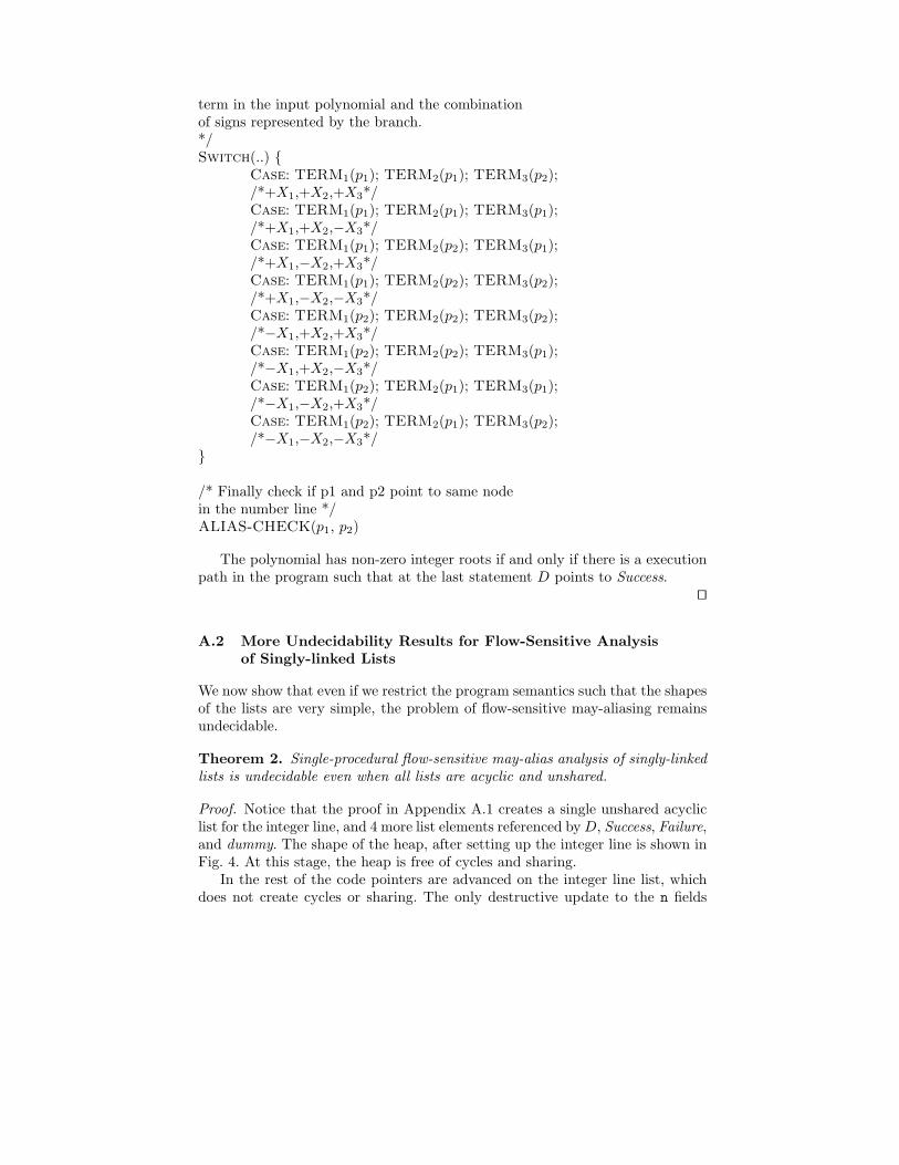
Proof. Notice that the proof in Appendix A.1 creates a single unshared acycliclist for the integer line, and 4 more list elements referenced byD, Success, Failure,and dummy. The shape of the heap, after setting up the integer line is shown inFig. 4. At this stage, the heap is free of cycles and sharing.

In the rest of the code pointers are advanced on the integer line list, whichdoes not create cycles or sharing. The only destructive update to the n fields

…

Zero

D Success

Failuredummy

temp

Fig. 4. The shape of the heap after setting up the integer line

happens in ALIAS-CHECK which could actually result in making D.n anddummy.n point to Failure and thus create sharing.

To see this, consider the situation where ALIAS-CHECK is first applied toaliased pointers. This makes D point to Failure. Then, if ALIAS-CHECK isapplied to a pair of non-aliased pointers then dummy is made to point to Failure.

In order to avoid creating this sharing, we slightly alter the ALIAS-CHECK

macro:

ALIAS-CHECK(A,B) :temp1 = A.n;temp2 = B.n;A.n = D;B.n = dummy;A.n.n = null;A.n = temp1;B.n = temp2

The change from ALIAS-CHECK is that instead of using the cell referencedby Failure, we are setting A.n.n to null. Since it is okay for two list elements torefer to null without creating sharing this solves the problem.

To see that no sharing is created during the application of the revised ALIAS-

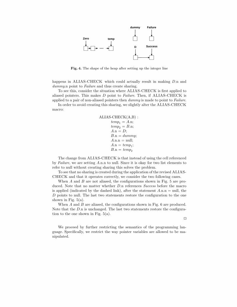
CHECK and that it operates correctly, we consider the two following cases.When A and B are not aliased, the configurations shown in Fig. 5 are pro-

duced. Note that no matter whether D.n references Success before the macrois applied (indicated by the dashed link), after the statement A.n.n = null, theD points to null. The last two statements restore the configuration to the oneshown in Fig. 5(a).

When A and B are aliased, the configurations shown in Fig. 6 are produced.Note that the D.n is unchanged. The last two statements restore the configura-tion to the one shown in Fig. 5(a).

⊓⊔

We proceed by further restricting the semantics of the programming lan-guage. Specifically, we restrict the way pointer variables are allowed to be ma-nipulated.

Zero

D Success

dummy

tempA Btmp1 tmp2

………

Zero

D Success

dummy

tempA Btmp1 tmp2

… ……

(a) (b)

…

Zero

D Success

dummy

tempA Btmp1 tmp2

…… …

Zero

D Success

dummy

tempA Btmp1 tmp2

……

(c) (d)

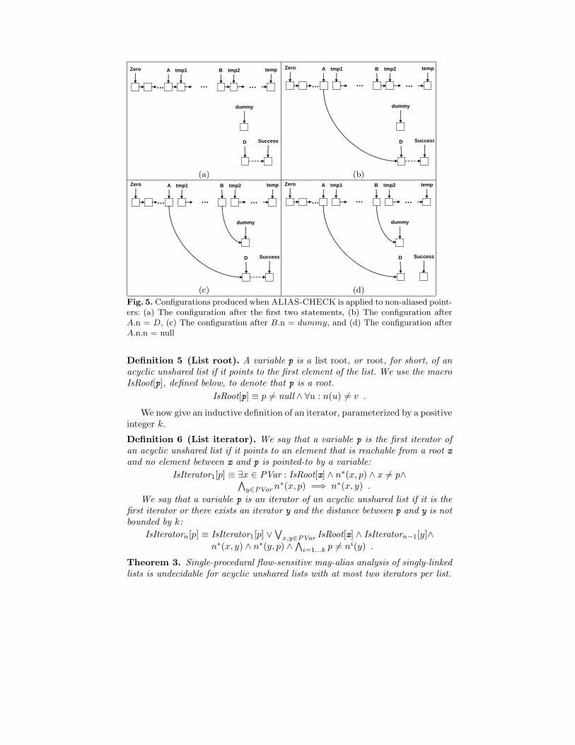
Fig. 5. Configurations produced when ALIAS-CHECK is applied to non-aliased point-ers: (a) The configuration after the first two statements, (b) The configuration afterA.n = D, (c) The configuration after B.n = dummy, and (d) The configuration afterA.n.n = null

Definition 5 (List root). A variable p is a list root, or root, for short, of anacyclic unshared list if it points to the first element of the list. We use the macroIsRoot[p], defined below, to denote that p is a root.

IsRoot[p] ≡ p 6= null ∧ ∀u : n(u) 6= v .

We now give an inductive definition of an iterator, parameterized by a positiveinteger k.

Definition 6 (List iterator). We say that a variable p is the first iterator ofan acyclic unshared list if it points to an element that is reachable from a root xand no element between x and p is pointed-to by a variable:

IsIterator1[p] ≡ ∃x ∈ PVar : IsRoot[x] ∧ n∗(x, p) ∧ x 6= p∧∧

y∈PVar n∗(x, p) =⇒ n∗(x, y) .

We say that a variable p is an iterator of an acyclic unshared list if it is thefirst iterator or there exists an iterator y and the distance between p and y is notbounded by k:

IsIteratorn[p] ≡ IsIterator1[p] ∨∨

x,y∈PVar IsRoot[x] ∧ IsIteratorn−1[y]∧n∗(x, y) ∧ n∗(y, p) ∧ ∧

i=1...k p 6= ni(y) .

Theorem 3. Single-procedural flow-sensitive may-alias analysis of singly-linkedlists is undecidable for acyclic unshared lists with at most two iterators per list.

Zero

D Success

dummy

tempA B tmp1 tmp2

…

Zero

D Success

dummy

tempA B tmp1 tmp2

…

(a) (b)Zero

D Success

dummy

tempA B tmp1 tmp2

…

Zero

D Success

dummy

tempA B tmp1 tmp2

…

(c) (d)

Fig. 6. Configurations produced when ALIAS-CHECK is applied to aliased pointers:(a) The configuration after the first two statements, (b) The configuration after A.n =D, (c) The configuration after B.n = dummy, and (d) The configuration after A.n.n= null

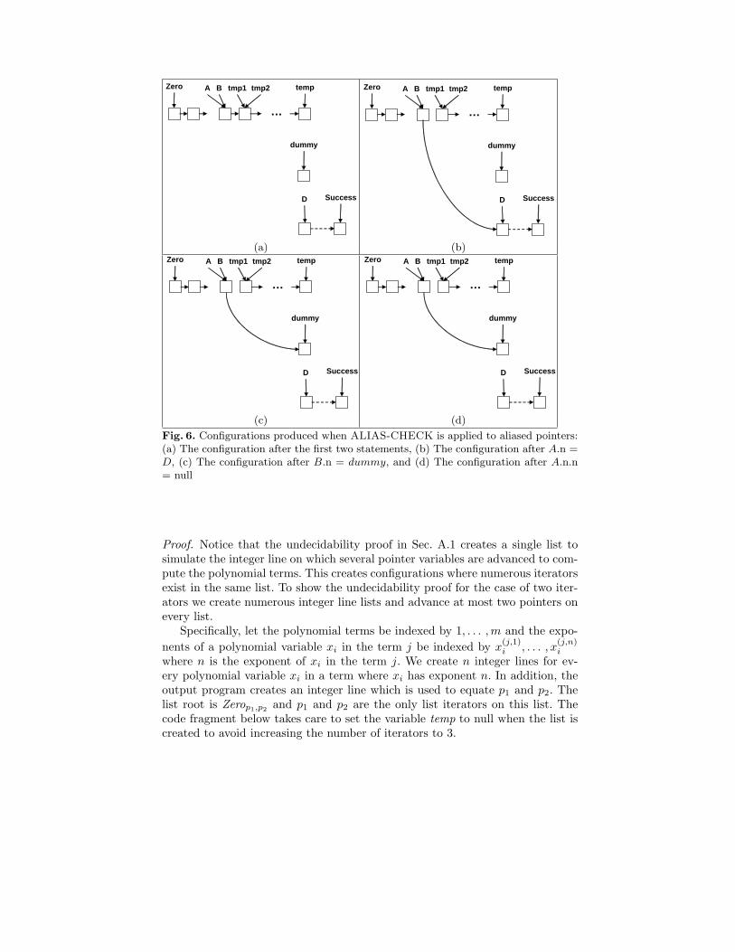
Proof. Notice that the undecidability proof in Sec. A.1 creates a single list tosimulate the integer line on which several pointer variables are advanced to com-pute the polynomial terms. This creates configurations where numerous iteratorsexist in the same list. To show the undecidability proof for the case of two iter-ators we create numerous integer line lists and advance at most two pointers onevery list.

Specifically, let the polynomial terms be indexed by 1, . . . ,m and the expo-

nents of a polynomial variable xi in the term j be indexed by x(j,1)i , . . . , x

(j,n)i

where n is the exponent of xi in the term j. We create n integer lines for ev-ery polynomial variable xi in a term where xi has exponent n. In addition, theoutput program creates an integer line which is used to equate p1 and p2. Thelist root is Zerop1,p2

and p1 and p2 are the only list iterators on this list. Thecode fragment below takes care to set the variable temp to null when the list iscreated to avoid increasing the number of iterators to 3.

Success = new List();dummy = new List();D = new List();D.n = Success;Zerop1,p2

= temp = new List();While(..) {

temp.n = new List(); temp = temp.n;/* Create an integer line for every indexed polynomial variable (i, j) */...temp(i,j).n = new List(); temp(i,j) = temp(i,j).n;

...}temp = null...temp(i,j) = null

...

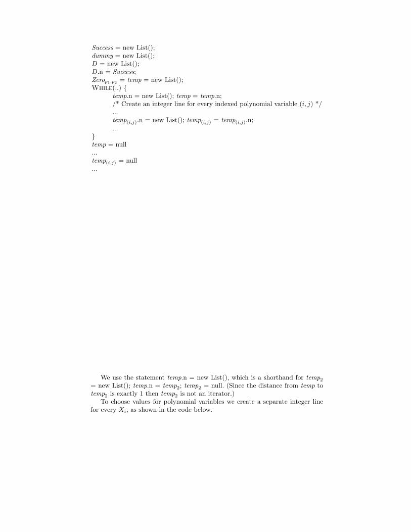
We use the statement temp.n = new List(), which is a shorthand for temp2

= new List(); temp.n = temp2; temp2 = null. (Since the distance from temp totemp2 is exactly 1 then temp2 is not an iterator.)

To choose values for polynomial variables we create a separate integer linefor every Xi, as shown in the code below.

X1 = Zero1 = new List();

X(1,1)1 = Zero

(1,1)1

While(..){X1.n = new List(); X1 = X1.n;

X(1,1)1 = X

(1,1)1 .n

X(2,1)1 = X

(2,1)1 .n

}X2 = Zero2 = new List();

X(2,2)2 = Zero

(2,2)2 = new List();

X(3,1)2 = Zero

(3,1)2 = new List();

While(..) {X2.n = new List(); X2 = X2.n;

X(2,2)2 = X

(2,2)2 .n

X(3,1)2 = X

(3,1)2 .n

}X3 = Zero3 = new List();

X(3,1)3 = Zero

(3,1)3 = newList();

X(3,2)3 = Zero

(3,2)3 = newList();

While(..) {X3.n = new List(); X3 = X3.n;

X(3,1)3 = X

(3,1)3 .n

X(3,2)3 = X

(3,2)3 .n

}

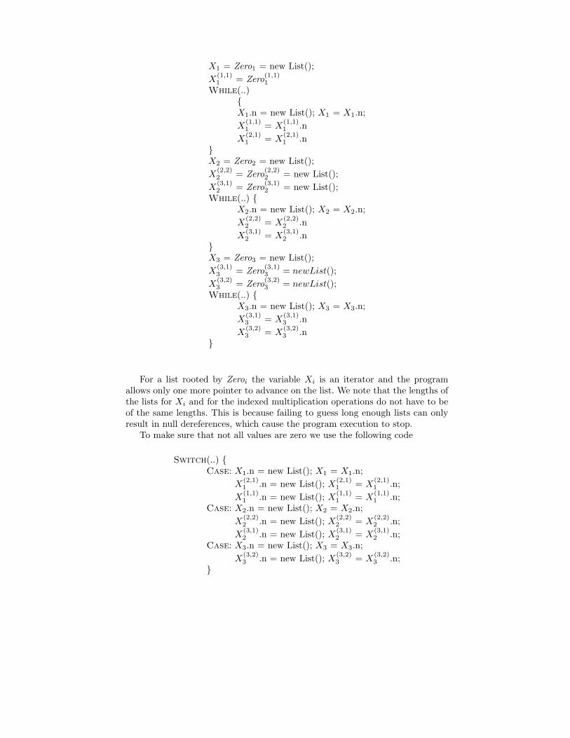
For a list rooted by Zeroi the variable Xi is an iterator and the programallows only one more pointer to advance on the list. We note that the lengths ofthe lists for Xi and for the indexed multiplication operations do not have to beof the same lengths. This is because failing to guess long enough lists can onlyresult in null dereferences, which cause the program execution to stop.

To make sure that not all values are zero we use the following code

Switch(..) {Case: X1.n = new List(); X1 = X1.n;

X(2,1)1 .n = new List(); X

(2,1)1 = X

(2,1)1 .n;

X(1,1)1 .n = new List(); X

(1,1)1 = X

(1,1)1 .n;

Case: X2.n = new List(); X2 = X2.n;

X(2,2)2 .n = new List(); X

(2,2)2 = X

(2,2)2 .n;

X(3,1)2 .n = new List(); X

(3,1)2 = X

(3,1)2 .n;

Case: X3.n = new List(); X3 = X3.n;

X(3,2)3 .n = new List(); X

(3,2)3 = X

(3,2)3 .n;

}

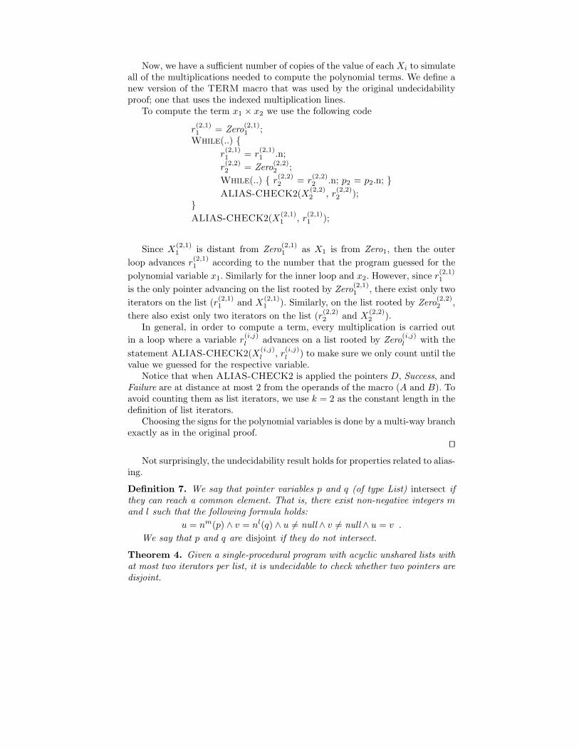
Now, we have a sufficient number of copies of the value of each Xi to simulateall of the multiplications needed to compute the polynomial terms. We define anew version of the TERM macro that was used by the original undecidabilityproof; one that uses the indexed multiplication lines.

To compute the term x1 × x2 we use the following code

r(2,1)1 = Zero

(2,1)1 ;

While(..) {r(2,1)1 = r

(2,1)1 .n;

r(2,2)2 = Zero

(2,2)2 ;

While(..) { r(2,2)2 = r

(2,2)2 .n; p2 = p2.n; }

ALIAS-CHECK2(X(2,2)2 , r

(2,2)2 );

}ALIAS-CHECK2(X

(2,1)1 , r

(2,1)1 );

Since X(2,1)1 is distant from Zero

(2,1)1 as X1 is from Zero1, then the outer

loop advances r(2,1)1 according to the number that the program guessed for the

polynomial variable x1. Similarly for the inner loop and x2. However, since r(2,1)1

is the only pointer advancing on the list rooted by Zero(2,1)1 , there exist only two

iterators on the list (r(2,1)1 and X

(2,1)1 ). Similarly, on the list rooted by Zero

(2,2)2 ,

there also exist only two iterators on the list (r(2,2)2 and X

(2,2)2 ).

In general, in order to compute a term, every multiplication is carried out

in a loop where a variable r(i,j)l advances on a list rooted by Zero

(i,j)l with the

statement ALIAS-CHECK2(X(i,j)l , r

(i,j)l ) to make sure we only count until the

value we guessed for the respective variable.Notice that when ALIAS-CHECK2 is applied the pointers D, Success, and

Failure are at distance at most 2 from the operands of the macro (A and B). Toavoid counting them as list iterators, we use k = 2 as the constant length in thedefinition of list iterators.

Choosing the signs for the polynomial variables is done by a multi-way branchexactly as in the original proof.

⊓⊔Not surprisingly, the undecidability result holds for properties related to alias-

ing.

Definition 7. We say that pointer variables p and q (of type List) intersect ifthey can reach a common element. That is, there exist non-negative integers mand l such that the following formula holds:

u = nm(p) ∧ v = nl(q) ∧ u 6= null ∧ v 6= null ∧ u = v .

We say that p and q are disjoint if they do not intersect.

Theorem 4. Given a single-procedural program with acyclic unshared lists withat most two iterators per list, it is undecidable to check whether two pointers aredisjoint.

Proof. This follows immediately from the proof of Theorem 3, since D.n andSuccess intersect if and only if they are aliased. ⊓⊔

B Deriving Optimal Abstract Transformers for Program

Statements

In this section we derive abstract transformers for the different types of programstatements. We describe the criteria for which these transformers are optimaland supply proofs.

Outline. The rest of this section is organized as follows. In Subsection B.1we supply definitions and notations used in the rest of this section. In Subsec-tion B.2 we describe a technique that can be used for deriving complete abstracttransformers for certain program statements. In Subsection B.3 we describe atechnique that can be used for deriving the best abstract transformers for cer-tain program statements. In Subsection B.4 we define a variant of the best trans-former and give sufficient conditions under which the the analysis using the vari-ant of the best transformer and the analysis using the best transformer yield thesame results. In Subsection B.5 we explain how to use a known result to updatereachability predicates. In Subsection B.6 we show how to derive a complete ab-stract transformer for statements of the form x=new List(). In Subsection B.7we show how to derive a complete abstract transformer for statements of theform x.n=null. In Subsection B.8 we show how to derive a complete abstracttransformer for statements of the form x.n=y. In Subsection B.9 we show howto derive the best abstract transformer for statements of the form x=y.n.

The derivation of complete abstract transformers for the statements of theform x=null and x=y is straightforward, and thus we omit the details.

B.1 Preliminaries

��

’st÷

� ’st÷��

�’

�’α’

� ’st÷#

α’

�’Fig. 7. A pair of commutative diagrams showing the relations between the concretesemantics, the instrumented semantics, and the abstract semantics

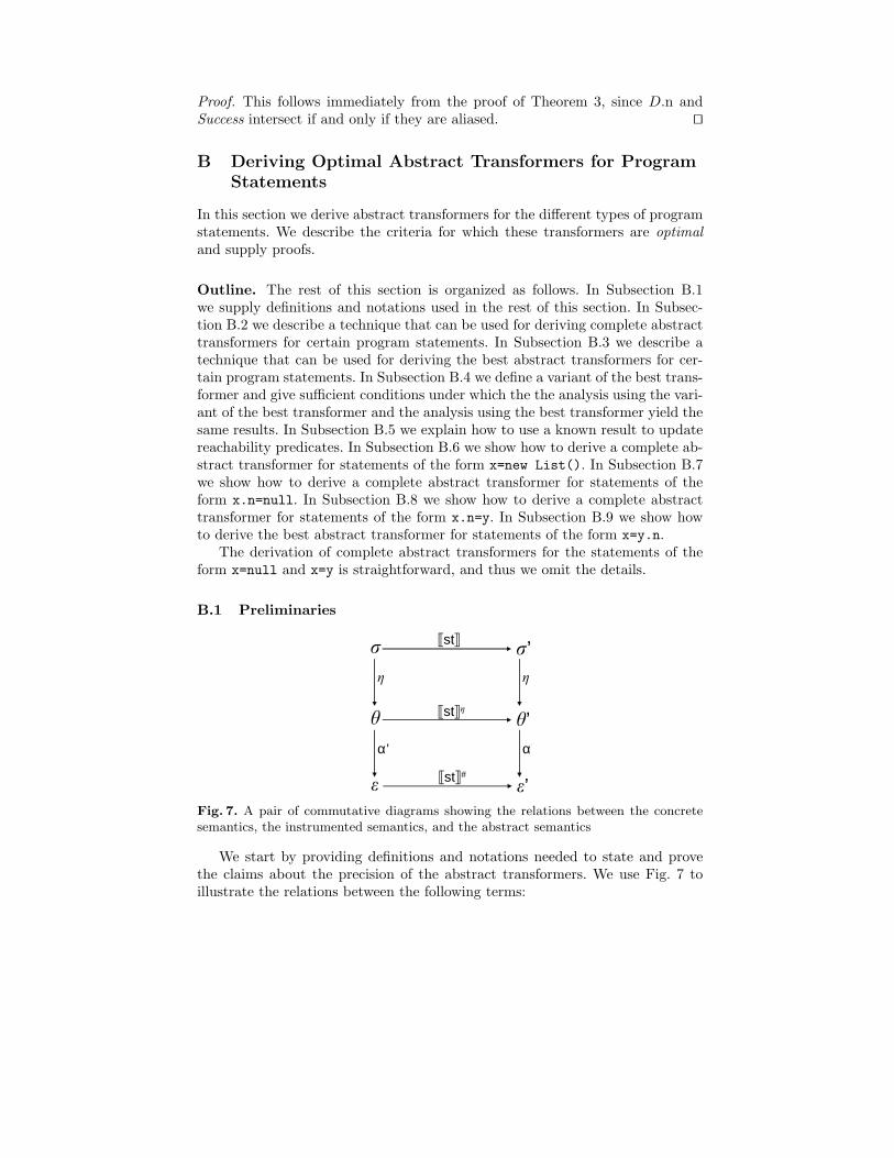
We start by providing definitions and notations needed to state and provethe claims about the precision of the abstract transformers. We use Fig. 7 toillustrate the relations between the following terms:

Concrete states The set of symbols τ = PVar ∪ {n} is used to define func-tions over list elements. For convenience of notation we shall also refer to anindexed version of the functions in τ by f1, . . . , fm.A concrete state is a first-order structure σ = (U, I) where U is a set ofindividuals (list elements) and I is a function that interprets symbols inτ . The symbols in PVar are constants, i.e., I maps every symbol to anindividual in U (representing either an allocated list element or the nullelement). The symbol n is interpreted by I as a function U → U .

Concrete semantics We separate the set of statements into two classes: (a)mutating statements, which include x=null, x=new List(), x=y, x.n=null,x.n=y, and x=y.n; and filtering statements, which include assume statementsand assert statements.The concrete operational semantics specifies how a mutating statement trans-forms a concrete state σ = (U, I) into a new concrete state σ′ = (U ′, I ′) =[[st]](σ). This is done by using a first-order formula ψi to relate the interpre-tation of the symbol fi ∈ τ in I ′ to the interpretation of the symbol fi ∈ τ inI, for every i = 1, . . . ,m. In this paper, the update formulae for the concreteoperational semantics are specified in Table 1. We specify the update to theset of elements U directly — U ′ is either U or U ′ = U ∪ {vnew} where vnew

is a fresh element.The semantics of assume statements and assert statements is given by stateformulae that act as conditions. When the condition holds, the output stateis identical to the input state. When the condition fails, the output is thespecial state ⊥, which intuitively means that execution has stopped (in theset extension of the semantics we drop bottom states).The operational semantics is extended to operate on sets of concrete statesby using set union to join the effect of the semantics on individual states:

[[st ]](XS) = {[[st ]](σ) | σ ∈ XS} \ {⊥} .

Instrumented States We extend the vocabulary of every concrete state tocontain a set of derived state predicates P = {P1 , . . . ,Pn}, υ = τ ∪ P . Thevalue of every predicate Pi ∈ P in an instrumented state is defined by a stateformula φi specified in first-order logic with transitive closure.In this paper, the set of predicates P and the corresponding defining formulaeare specified in Table 2.We denote by η the function that maps a concrete state σ to an instrumentedstate θ where the interpretation of each predicate Pi ∈ P is obtained byevaluating its defining formula φi in σ.

Instrumented semantics The instrumented semantics of a program state-ment st maps an instrumented state θ to θ′ = [[st]]η(θ) by using the concretesemantics to update the interpretation of the concrete symbols (in τ), andusing first-order formulae over the symbols in υ to update the predicatesin P . We denote by µi the formula used by the instrumented semantics toupdate the predicate Pi ∈ P . The updates to the predicates in P yield a com-mutative diagram (shown in the upper part of Fig. 7). That is, the followingequation holds.

η ◦ [[st]] = [[st]]η ◦ η . (1)

Abstract states The abstraction of an instrumented state θ is obtained byprojection on the predicates in P , which are therefore referred to as abstrac-tion predicates. Formally, ε = α′(θ) = 〈b1, . . . , bn〉 where bi is a (proposition)Boolean variable and bi = [[Pi]]

θ for i = 1, . . . , n. In logical form, the abstractstate is the cube

∧

Pi∈P P̃i, where P̃i = Pi when bi = 1 and P̃i = ¬Pi whenbi = 0. The abstraction of a concrete state σ is ε = α(η(σ)), i.e., α = α′ ◦ η.The abstraction of a set of states (concrete states or instrumented states)is the set of abstract states obtained from the abstraction of the individualstates.Note that we do not consider trivial cubes, i.e., cubes that do not representany concrete state, to be valid abstract states. This is justified by Theorem 8.We use the subset relation to define a partial order relation ⊑ on sets. Thisis a standard definition in predicate abstraction.

Abstract semantics In contrast to the concrete semantics and instrumentedsemantics, where a single input state is mapped to a single output state,the abstract semantics of a program statement st is a function from abstractstates to sets of abstract states. Given an abstract state ε, the value of apredicate Pi in each output state ε′ ∈ [[st]]#(ε) is specified by an updateformula that is a Boolean function, δi, over the variables {bi}n

i=1 in ε. (Inorder to reduce notational overhead we do not introduce the variables {bi}n

i=1

but rather use the names of the corresponding predicates.)The update formulae for the mutating statements x=null, x=new List(),x=y, x.n=null, and x.n=y are given in Table 3. For these statements, theabstract transformer maps a single abstract state to a single abstract state(a singleton set), resulting with the commutative diagram shown in the lowerpart of Fig. 7,

α′ ◦ [[st]]η = [[st]]# ◦ α′ . (2)

The abstract semantics of filtering statements is specified by a Boolean func-tion over the predicates in P , as shown in Table 3. In the sequel, we provethat the abstract semantics is complete for these statements.The abstract semantics for statements of the form x=y.n is incomplete, re-sulting by either 1 or 2 abstract states, as specified in Fig. 3. However, theabstract transformer is the most precise, i.e., the best transformer for thisstatement.We extend the abstract semantics of a program statement to operate on setsof abstract states by taking the point-wise extension of the semantics onsingle abstract states, i.e., the set union of the semantics on each abstractstate.

B.2 A Methodology for Deriving Complete Abstract Transformers

We now define what it means for an abstract transformer of a statement to becomplete for a given abstraction.

Definition 8 (Completeness of an abstract transformer). Let st be a pro-gram statement. An abstract transformer [[st]]# is said to be complete when the

following holds

α ◦ [[st]] = [[st]]# ◦ α .

We say that an abstract transformer [[st]]# is sound when α([[st]](XS)) ⊑[[st]]#(α(XS)) holds for every set of concrete states XS.

Whether a complete abstract transformer exists for a program statementdepends on the given abstraction. The following proposition supplies a negativetest for completeness, i.e., it gives a way of showing that no abstract transformeris complete for a given program statement and a given abstraction.

Proposition 2. Let [[st]]# be a sound abstract transformer for a statement st.The transformer [[st]]# is complete if and only if every abstract state ε is mappedto a single abstract state.

Proof. By contradiction. Assume that [[st]]# is a complete abstract transformerand let ε be an abstract state such that [[st]]#(ε) contains two distinct abstractstates.

Now, let σ be a concrete state such that α(σ) = ε. Then, σ′ = [[st]](σ) isanother concrete state (possibly ⊥). Now, α({σ′}) = {ε′}\{⊥} where ε′ = α(σ′)is a single abstract state. We arrived to a contradiction since |α({σ′})| ≤ 1, andthus [[st]]#(α(σ)) 6= α([[st]](σ)). ⊓⊔

In order to show that no abstract transformer is complete for a given programstatement and a given abstraction, we need to show that there exist two concretestates σ1 and σ2 such that α(σ1) = α(σ2) and α([[st]](σ1)) 6= α([[st]](σ2)).

The following two theorems give sufficient conditions for showing that a com-plete abstract transformer exists for a given statement and predicate abstraction.

Theorem 5. Let st be a mutating program statement.If for every predicate in P, the update formulae {µi}n

i=1 used by the instru-mented semantics are Boolean functions over the current state predicates in P,then the abstract transformer [[st]]# where λi = µi for i = 1, . . . , n is complete.

Proof. Recall that the instrumented semantics, by definition, induces a commu-tative diagram, as expressed by Equation 1.

Since λi = µi for i = 1, . . . , n, and the update formulae depend only on theabstraction predicates, Equation 2 (α′ ◦ [[st]]η = [[st]]# ◦ α′) holds.

We can now compose the two commutative diagrams, as shown in Fig. 7, andobtain the desired claim:

[[st]]# ◦ α =[[st]]# ◦ α′ ◦ η =(Since α = α′ ◦ η)α′ ◦ [[st]]η ◦ η =(Using Equation 2)α′ ◦ η ◦ [[st]] =(Using Equation 1)α ◦ [[st]](Since α = α′ ◦ η) .

⊓⊔

Theorem 6. Let st be a filtering statement. If the condition can be expressedby a Boolean function over the predicates in P then the corresponding abstracttransformer is complete.

Proof. This immediately follows since the condition formula is expressed byequivalent formulae over the predicates. ⊓⊔

In this paper, the conditions in assume and assert statements can be ex-pressed by the abstraction predicates (see Table 3). Therefore, by Theorem 6,the abstract transformers are complete for these statements.

For mutating statements we show the completeness of the abstract trans-formers by using Theorem 5 in the following way. The state α′ ◦ [[st]] is

〈[[φ1]]σ′

, . . . , [[φk]]σ′〉 .

The state [[st]]η ◦ α′ is given by

〈µ1(P1, . . . , Pn), . . . , µk(P1, . . . , Pn)〉 .To show that the two terms are equal, we show that

[[φi]]σ′ ⇐⇒ µi(P1, . . . , Pn)

holds for every i = 1, . . . , k.To show this, we use folding/unfolwing transformations:

1. Unfolding the defining formula of the post-state predicate We startby writing the formula φi using the primed versions of the symbols in τ(representing [[φi]]

σ′

).2. Unfolding the concrete semantics We use the fact that the set of individ-

uals does not change (this is true for all mutating statements, except x=newList()) and substitute the concrete concrete update formulae (from Table 1)with the corresponding symbols from the concrete vocabulary to obtain theformula φi[ψi/P1, . . . , ψn/P1]. This formula contains only current-state (un-primed) symbols.

3. Equivalence-preserving Transformations We apply transformations thatpreserve the equivalence of formulae for our set of models.

4. Folding The last transformation results in a Boolean function over thecurrent-state abstraction predicates, which is identical to µi(b1, . . . , bn).

For statements of the form x=new List(), the second step cannot be applieddirectly, since the set of individuals changes. However, most of the state remainsunchanged by the allocation statement, which allowing us to apply reasoningspecific to this statement to show that the commutativity condition holds.

B.3 A Methodology for Deriving Best Abstract Transformers

We now describe a technique for showing that an incomplete abstract trans-former is the most precise. Intuitively, the technique is based on finding formu-lae that allow to conduct a case analysis. In each case, we use the techniquedescribed in the previous subsection to derive a complete transformer. In addi-tion, there is a proof obligation for showing that every abstract state representsconcrete states for all cases. We proceed by formally defining the notion of casesplitting.

Definition 9 (Focus formulae). Let Pfocus be a predicate with the associateddefining formula φfocus such that for every concrete state σ1, there exists a con-crete state σ2 such that: (a) α(σ1) = α(σ2); and (b) either σ1 |= φfocus andσ2 |= ¬φfocus or σ2 |= φfocus and σ1 |= ¬φfocus.

We call Pfocus a focus predicate and φfocus a focus formula.

The next theorem supplies sufficient conditions for which a single focus for-mula can be used to define the best transformer, i.e., there are only two cases.The generalization to more than two cases, where several focus formulae areneeded to perform the case splitting, is simple.

Theorem 7. Let st be a mutating statement.Let Pfocus and φfocus be a focus predicate and the associated focus formula,

respectively.Assume that the update formulae δi can be expressed by a Boolean function

over the predicates in P and Pfocus for every i = 1, . . . , n (notice that we do noupdate Pfocus itself as it is only needed for the case splitting).

Let µ0i be δi[0/Pfocus] and let µ1

i be δi[1/Pfocus] for i = 1, . . . , n. Let [[st]]#0be the transformer defined via the update formulae {µ0

i }ni=1, and let [[st]]#1 be the

transformer defined via the update formulae {µ1i }n

i=1.We define the following abstract transformer. Given an abstract state ε,

[[st]]#(ε) = {[[st]]#0 (ε), [[st]]#1 (ε)} .

That is, the output consists of two cubes where the update formulae are theones used by the instrumented semantics and the value of Pfocus is set non-deterministically to 0 and 1.

The abstract transformer [[st]]# defined above is the best transformer for st.

Proof. Let [[st]]b be the best transformer for the mutating statement st8 and let[[st]]# be the abstract transformer defined above. We have to show two things:(i) the abstract transformer [[st]]# is sound, i.e., α([[st]](σ)) ⊑ [[st]]#(α(σ)) holdsfor every concrete state σ; and (ii) the transformer is as precise as the best, i.e.,[[st]]#(α(σ)) ⊑ [[st]]b(α(σ)) holds for every concrete state σ. (These two propertiesdirectly extend to sets of concrete states.)

Let σ be a concrete state such σ |= φfocus. The instrumented state θ = η(σ)also satisfies φfocus. Therefore, [[µ1

i ]]θ = [[δi]]

θ for i = 1, . . . , n, and thus thefollowing equation holds

α′([[st]]η(θ)) = [[st]]#1 (α′(θ)) .

Now, notice that, for every concrete state that satisfies φfocus, we have twocommutative diagrams, as shown in Fig. 7, which means that the transformer[[st]]#1 is complete for this set of states. (This is the same reasoning used in the

proof of Theorem 5). Similarly, the transformer [[st]]#0 is complete for the set ofstates that satisfy ¬φfocus.

Since every concrete state satisfies either φfocus or ¬φfocus, we have thatα([[st]](σ)) ∈ [[st]]#(α(σ)) holds for every concrete state. Thus, α([[st]](σ)) ⊑[[st]]#(α(σ)), which shows that the abstract transformer [[st]]# is sound.

8 The best abstract transformer is known to exist for every predicate abstraction.

Assume that σ |= φfocus (the proof for the case where σ |= ¬φfocus is sym-

metric). Recall that [[st]]#(α(σ)) = {[[st]]#0 (α(σ)), [[st]]#1 (α(σ))}. To show that

[[st]]#(α(σ)) ⊑ [[st]]b(α(σ)) holds we have to show that both [[st]]#0 (α(σ)) ∈[[st]]b(α(σ)) and [[st]]#1 (α(σ)) ∈ [[st]]b(α(σ)) hold.

Now, since [[st]]#1 (α(σ)) = α([[st]](σ)) holds and the best transformer is sound,

we have that [[st]]#1 (α(σ)) ∈ [[st]]b(α(σ)) holds.Since φfocus is a focus formula, there exists a state σ′ such that σ′ |= ¬φfocus

and α(σ) = α(σ′). From the fact α(σ) = α(σ′), we have that the followingequation holds

[[st]]b(α(σ)) = [[st]]b(α(σ′)) . (3)

From the fact σ′ |= ¬φfocus, we have that the following equation holds

α([[st]](σ′)) = [[st]]#0 (α(σ′)) . (4)

Since [[st]]b is a sound abstract transformer we have that the following holds

α([[st]](σ′)) ∈ [[st]]b(α(σ′)) . (5)

Combining Equation 5 and Equation 3 we obtain

α([[st]](σ′)) ∈ [[st]]b(α(σ)) . (6)

Combining Equation 6 and Equation 4 we obtain

[[st]]#0 (α(σ′)) ∈ [[st]]b(α(σ)) . (7)

Now, since [[st]]#0 (α(σ′)) = [[st]]#0 (α(σ)), we can rewrite Equation 7 and obtain

[[st]]#0 (α(σ)) ∈ [[st]]b(α(σ)) . (8)

⊓⊔

B.4 A Variant of the Best Transformer

We now define a variant of the best transformer and show that, under reasonableassumptions, the set of abstractly reachable states is the same as the set of statesthat are abstractly reachable with the best transformer.

Let [̃[st]]# be an abstract transformer, such that for every cube a, if γ(a) 6= ∅then [̃[st]]#(a) = [[st]]#(a). That is, [̃[st]]# identifies with [[st]]# on input cubes thatrepresent at least one concrete state.

Theorem 8. Let Sa be a set of cubes such that ∀a ∈ Sa : γ(a) 6= ∅. Then, theset of abstract states that are reachable from Sa by the transition relation induced

by [[st ]]# is the set of states reachable by the transition relation induced by [̃[st]]#.In other words, for every sequence of statements st1, . . . , stk, the following

holds:

[[stk]]# ◦ . . . ◦ [[st1]]#(sa) = [̃[stk]]# ◦ . . . ◦ [̃[st1]]#(sa) .

Proof. We know that the claim holds for a single statement. It suffices to provethat if a is a cube a such that a 6= ∅ then γ(b) 6= ∅ for every cube b ∈ [[st]]#(a).The rest of the proof is by induction on the length the sequence of statements.

Let a be a cube such that γ(a) 6= ∅. Let [[st]](γ(a)) be the set of concrete statesthat result from application of the concrete transformer to the concrete states

represented by a. If [[st]](γ(a)) is the empty set, then [[st]]#(a) = {α(ta) | ta ∈[[st]](γ(a))} = ∅, and the claim holds vacuously (there are no output cubes).If [[st]](γ(a)) is not empty then [[st]]#(a) = {α(ta) | ta ∈ [[st]](γ(a))} is the setof cubes mapped by α from some concrete state in [[st]](γ(a)). Therefore, everycube represents at least the concrete states mapped to it and therefore applyingγ to the cube returns a non-empty set, and thus the claim holds for all outputcubes. ⊓⊔

Thus, under the assumption that the set of input cubes does not containtrivial cubes (cubes that do not represent any concrete states), our transformersidentify with the best transformers. Since the logic we use is decidable, thisassumption can also be enforced, i.e., we can check whether a cube is non-trivial.For the benchmarks we used, the input cubes were produced from combinationsof lists pointed-to by single variables:

NotNull[x] ∧ NextNull[x],NotNull[x] ∧ ¬NextNull[x] ,

and thus the cubes are non-trivial.

B.5 Using the Dong and Su Reachability Update Formulae

In the construction of the update formulae for x.n=null and x.n=y, we usethe fact that REACH(acyclic) ∈ DynFO [10] (Theorem 14.20, pages 230–231),originally shown by Dong and Su [8]. This result lets us update the path predicateP , which is the reflexive-transitive closure of an acyclic relation E, using thefollowing first-order formulae:

Edge insertion When an edge (a, b) is added to the graph, the update to thepath predicate is given by

P ′(x, y) := P (x, y) ∨ (P (x, a) ∧ P (b, y)) . (9)

Edge deletion When an edge (a, b) is deleted from the graph, the update tothe path predicate is given by

P ′(x, y) := P (x, y) ∧[

¬(P (x, a) ∧ P (b, y))∨(∃u v)

(

P (x.u) ∧ E(u, v) ∧ P (v, y)∧P (u, a) ∧ ¬P (v, a) ∧ (a 6= u ∨ b 6= v)

)]

.(10)

We use these formulae to obtain the following two lemmas.

Lemma 1. For every four list elements x, y, w, and z, such that x 6= null,z 6= null, w 6= null, x 6= y, and n(x) = null hold , the following holds.

(λ v . (v = x?y : n(v)))+(w, z) ⇐⇒ n+(w, z) ∨ n∗(w, x) ∧ n∗(y, z) (11)

Proof. First, if y is null we have

(λ v . (v = x?y : n(v)))+(w, z) ⇐⇒ (λ v . (v = x?null : n(v)))+(w, z)

But, since n(x) = null we have

(λ v . (v = x?null : n(v)))+(w, z) ⇐⇒ n+(w, z) .

On the other hand,

n+(w, z) ∨ n∗(w, x) ∧ n∗(y, z) ⇐⇒ n+(w, z) ∨ n∗(w, x) ∧ n∗(null, z) .

Since z 6= null, we have n∗(null, z) = 0 and thus

n+(w, z) ∨ n∗(w, x) ∧ n∗(null, z) ⇐⇒ n+(w, z) .

Therefore, the equivalence holds in the case of y = null.We now proceed to prove the equivalence in the case of y 6= null.Since the heaps we consider contain only acyclic lists, we can write

(λ v . (v = x?y : n(v)))+(w, z) ⇐⇒ (λ v . (v = x?y : n(v)))∗(w, z) ∧ w 6= z

We can now use Equation 9 and write

(λ v . (v = x?y : n(v))∗(w, z) ∧ w 6= z ⇐⇒(n∗(w, z) ∨ (n∗(w, x) ∧ n∗(y, z))) ∧ w 6= z .

Opening parenthesis, we get

(n∗(w, z) ∨ (n∗(w, x) ∧ n∗(y, z))) ∧ w 6= z ⇐⇒(n∗(w, z) ∧ w 6= z) ∨ (n∗(w, x) ∧ n∗(y, z) ∧ w 6= z) .

Now, n∗(w, z) ∧ w 6= z ⇐⇒ n+(w, z), and since heaps are acyclic and x 6= y, wealso have that n∗(w, x) ∧ n∗(y, z) =⇒ w 6= z, and therefore we can write

(n∗(w, z) ∧ w 6= z) ∨ (n∗(w, x) ∧ n∗(y, z) ∧ w 6= z) ⇐⇒n+(w, z) ∨ n∗(w, x) ∧ n∗(y, z) .

⊓⊔

Lemma 2. For list elements x, w, and z, such that x 6= null, z 6= null, andw 6= null holds, the following holds.

(λ v . (v = x?null : n(v)))+(w, z) ⇐⇒ n+(w, z) ∧ ¬(n∗(w, x) ∧ n+(x, z)) (12)

Proof. Since the heaps we consider are deterministic, we can simplify Equa-tion 10 to

P ′(x, y) := P (x, y) ∧ ¬(P (x, a) ∧ P (b, y)) .

Now, since we assumed all lists are acyclic,

(λ v . (v = x?null : n(v)))+(w, z) ⇐⇒ (λ v . (v = x?null : n(v)))∗(w, z) ∧ w 6= z .

Using the simplified version of Equation 10, where the deleted edge is (x, n(x)),we write

(λ v . (v = x?null : n(v)))∗(w, z) ∧ w 6= z ⇐⇒n∗(w, z) ∧ ¬(n∗(w, x) ∧ n∗(n(x), z)) ∧ w 6= z .

We use the assumption that all lists are acyclic and thus n∗(w, z) ∧ w 6= z ⇐⇒n+(w, z), and that n∗(n(x), z) ⇐⇒ n+(x, z), and write

n∗(w, z) ∧ ¬(n∗(w, x) ∧ n∗(n(x), z)) ∧ w 6= z ⇐⇒n+(w, z) ∧ ¬(n∗(w, x) ∧ n+(x, z)) .

⊓⊔

B.6 Deriving Update Formulae for x=new List()

We assume that this statement is preceded by the statements x=null.The interpretation of the symbols in PVar \ {x} is unaffected by the state-

ment. Therefore, the predicates of the form Aliased[w, z] and NotNull[z] retaintheir current values for every z ∈ PVar \ {x}.

Since vnew is a fresh cell, the links between other cells remain unaffected bythe statement. Therefore, Therefore, the predicates of the form Next[w, z] andReach[w, z] retain their current values for every z ∈ PVar \ {x}.

We shall use the fact that, following the application of the statement, forevery element u 6= vnew, ¬n′+(u, vnew) and ¬n′+(vnew, u) hold.

Assume that z ∈ PVar \ {x}.

NotNull[x]′ ⇐⇒ x′ 6= null(Unfolding the defining formula of NotNull[x]′)

⇐⇒ vnew 6= null(Unfolding the concrete semantics of x=y.n)

⇐⇒ 1(Since we assumed that vnew is fresh)

Next[x, z]′ ⇐⇒ x′ 6= null ∧ z′ 6= null ∧ n′(x′) = z′

(Unfolding the defining formula of Next[x, z]′)⇐⇒ vnew 6= null ∧ z 6= null ∧ (λ v . (v = vnew ? null : n(v)))(vnew) = z

(Unfolding the concrete semantics of x=new List())⇐⇒ 1 ∧ z 6= null ∧ null = z)

(λ application)⇐⇒ 0

(z 6= null and null = z Contradict each other)

Next[z, x]′ ⇐⇒ z′ 6= null ∧ x′ 6= null ∧ n′(z′) = x′

(Unfolding the defining formula of Next[z, x]′)⇐⇒ z′ 6= null ∧ vnew 6= null ∧ (λ v . (v = vnew ? null : n(v)))(z) = vnew

(Unfolding the concrete semantics of x=new List())⇐⇒ z 6= null ∧ 1 ∧ n(z) = vnew)

(λ application)⇐⇒ 0

(Since n(z) is an element in the pre-state and vnew is not)

NextNull[x]′ ⇐⇒ x′ 6= null ∧ n′(x′) = null(Unfolding the defining formula of NextNull[x]′)

⇐⇒ vnew 6= null ∧ λ v . (v = vnew ? null : n(v))(vnew) = null(Unfolding the concrete semantics of x=new List())

⇐⇒ 1 ∧ null = null)(λ application)

⇐⇒ 1

Reach[x, z]′ ⇐⇒ x′ 6= null ∧ z′ 6= null ∧ n′+(x′, z′)(Unfolding the defining formula of Reach[x, z]′)

⇐⇒ vnew 6= null ∧ z 6= null ∧ n′+(vnew, z)(Unfolding the concrete semantics of x=new List())

⇐⇒ 0(Since n′(vnew) = null and z 6= null)

Reach[z, x]′ ⇐⇒ z′ 6= null ∧ x′ 6= null ∧ n′+(z′, x′)(Unfolding the defining formula of Reach[z, x]′)

⇐⇒ z 6= null ∧ vnew 6= null ∧ n′+(z, vnew)(Unfolding the concrete semantics of x=new List())

⇐⇒ 0

(Since n′+(z, vnew) does not hold for any element)

B.7 Deriving Update Formulae for x.n=null

We assume the this statement is preceded by assert x != null, and thereforex 6= null holds.

Since the concrete semantics only changes the function n, the predicates ofthe form Aliased[w, z] and NotNull[z] retain their current values.

Assume that w, z ∈ PVar \ {x} and that w and z are different (Next[w, z] isdefined for different variables).

Next[w, z]′ ⇐⇒ w′ 6= null ∧ z′ 6= null ∧ n′(w′) = z′

(Unfolding the defining formula of Next[w, z]′)⇐⇒ w 6= null ∧ z 6= null ∧ (λ v.v = x?null : n(v))(w) = z

(Unfolding the concrete semantics of x.n=null)⇐⇒ w 6= null ∧ z 6= null ∧ (w = x ∧ z = null ∨ w 6= x ∧ n(w) = z)

(λ application)⇐⇒ w 6= null ∧ (z 6= null ∧ w 6= x ∧ n(w) = z)

(Distributing ∧ over ∨)⇐⇒ w 6= x ∧ w 6= null ∧ z 6= null ∧ n(w) = z

(Opening parenthesis and reordering terms)⇐⇒ ¬Aliased[w, x] ∧ Next[w, z]

(Folding)

When w is x, the step before folding yields 0, and therefore Next[x, z]′ = 0.When z is x, we continue from the last step before folding

Next[w, x]′ ⇐⇒ w 6= null ∧ w 6= x ∧ x 6= null ∧ n(w) = x⇐⇒ w 6= null ∧ x 6= null ∧ n(w) = x

(from Def. 1 we have that n(w) = x =⇒ w 6= x)⇐⇒ Next[w, x]

(Folding)

Assume that z ∈ PVar \ {x}.NextNull[z]′ ⇐⇒ z′ 6= null ∧ n′(z′) = null

(Unfolding the defining formula of NextNull[z]′)⇐⇒ z 6= null ∧ (λ v.v = x?null : n(v))(z) = null

(Unfolding the concrete semantics of x.n=null)⇐⇒ z 6= null ∧ (z = x ∧ null = null ∨ z 6= x ∧ n(z) = null)

(λ application)⇐⇒ z 6= null ∧ z = x ∨ z 6= null ∧ z 6= x ∧ n(z) = null

(Opening parenthesis)⇐⇒ z = x ∨ z 6= x ∧ z 6= null ∧ n(z) = null

(z = x and we assumed that x 6= null)⇐⇒ z = x ∨ z 6= null ∧ n(z) = null

(A ∨ ¬A ∧B ↔ A ∨B)⇐⇒ Aliased[z, x] ∨ NextNull[z]

(Folding)

When z is x the step before folding yields 1, and therefore NextNull[x]′ = 1.Assume that w, z ∈ PVar and that w and z are different (Reach[w, z] is

defined for different variables).

Reach[w, z]′ ⇐⇒ w′ 6= null ∧ z′ 6= null ∧ n′+(w′, z′)(Unfolding the defining formula of Reach[w, z]′)

⇐⇒ w 6= null ∧ z 6= null ∧ (λ v.v = x?null : n(v))+(w, z)(Unfolding the concrete semantics of x.n=null)

⇐⇒ w 6= null ∧ z 6= null ∧ n+(w, z) ∧ ¬(n∗(w, x) ∧ n+(x, z))(Lemma 2)

⇐⇒ Reach[w, z] ∧ ¬(ReachOrAliased[w, x] ∧ Reach[x, z])(x 6= null and folding)

When w is x, we get

Reach[x, z]′ ⇐⇒ x 6= null ∧ z 6= null ∧ n+(x, z) ∧ ¬(n∗(x, x) ∧ n+(x, z))(Lemma 2)

⇐⇒ x 6= null ∧ z 6= null ∧ n+(x, z) ∧ ¬n+(x, z)(n∗(x, x) always holds)

⇐⇒ 0

When z is x, we get

Reach[w, x]′ ⇐⇒ w 6= null ∧ x 6= null ∧ n+(w, x) ∧ ¬(n∗(w, x) ∧ n+(x, x))(Lemma 2)

⇐⇒ w 6= null ∧ x 6= null ∧ n+(w, x)(n+(x, x) does not hold since lists are acyclic)

⇐⇒ Reach[w, x](Folding)

B.8 Deriving Update Formulae for x.n=y

We assume the this statement is preceded by x.n = null, and therefore x 6= nulland n(x) = null hold. We also assume (and check) the following assumptions:(i) there are no incoming edges to y, i.e., ∀u : ¬n(u, y); and (ii) ¬n∗(y, x).

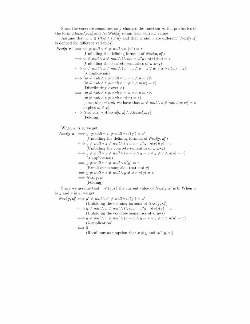
Since the concrete semantics only changes the function n, the predicates ofthe form Aliased[w, z] and NotNull[z] retain their current values.

Assume that w, z ∈ PVar \ {x, y} and that w and z are different (Next[w, z]is defined for different variables).

Next[w, z]′ ⇐⇒ w′ 6= null ∧ z′ 6= null ∧ n′(w′) = z′

(Unfolding the defining formula of Next[w, z]′)⇐⇒ w 6= null ∧ z 6= null ∧ (λ v.v = x?y : n(v))(w) = z

(Unfolding the concrete semantics of x.n=y)⇐⇒ w 6= null ∧ z 6= null ∧ (w = x ∧ y = z ∨ w 6= x ∧ n(w) = z)

(λ application)⇐⇒ (w 6= null ∧ z 6= null ∧ w = x ∧ y = z)∨

(w 6= null ∧ z 6= null ∧ w 6= x ∧ n(w) = z)(Distributing ∨ over ∧)

⇐⇒ (w 6= null ∧ z 6= null ∧ w = x ∧ y = z)∨(w 6= null ∧ z 6= null ∧ n(w) = z)(since n(x) = null we have that w 6= null ∧ z 6= null ∧ n(w) = zimplies w 6= x)

⇐⇒ Next[w, z] ∨ Aliased[w, x] ∧ Aliased[z, y](Folding)

When w is y, we get

Next[y, z]′ ⇐⇒ y′ 6= null ∧ z′ 6= null ∧ n′(y′) = z′

(Unfolding the defining formula of Next[y, z]′)⇐⇒ y 6= null ∧ z 6= null ∧ (λ v.v = x?y : n(v))(y) = z

(Unfolding the concrete semantics of x.n=y)⇐⇒ y 6= null ∧ z 6= null ∧ (y = x ∧ y = z ∨ y 6= x ∧ n(y) = z)

(λ application)⇐⇒ y 6= null ∧ z 6= null ∧ n(y) = z

(Recall our assumption that x 6= y)⇐⇒ y 6= null ∧ z 6= null ∧ y 6= x ∧ n(y) = z⇐⇒ Next[y, z]

(Folding)

Since we assume that ¬n∗(y, x) the current value of Next[y, x] is 0. When wis y and z is x, we get

Next[y, x]′ ⇐⇒ y′ 6= null ∧ x′ 6= null ∧ n′(y′) = x′

(Unfolding the defining formula of Next[y, x]′)⇐⇒ y 6= null ∧ x 6= null ∧ (λ v.v = x?y : n(v))(y) = x

(Unfolding the concrete semantics of x.n=y)⇐⇒ y 6= null ∧ x 6= null ∧ (y = x ∧ y = x ∨ y 6= x ∧ n(y) = x)

(λ application)⇐⇒ 0

(Recall our assumption that x 6= y and¬n∗(y, x))

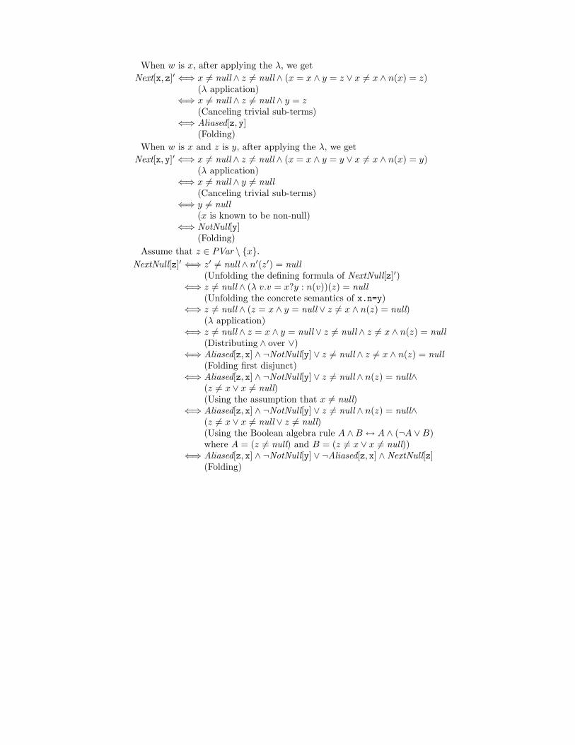
When w is x, after applying the λ, we get

Next[x, z]′ ⇐⇒ x 6= null ∧ z 6= null ∧ (x = x ∧ y = z ∨ x 6= x ∧ n(x) = z)(λ application)

⇐⇒ x 6= null ∧ z 6= null ∧ y = z(Canceling trivial sub-terms)

⇐⇒ Aliased[z, y](Folding)

When w is x and z is y, after applying the λ, we get

Next[x, y]′ ⇐⇒ x 6= null ∧ z 6= null ∧ (x = x ∧ y = y ∨ x 6= x ∧ n(x) = y)(λ application)

⇐⇒ x 6= null ∧ y 6= null(Canceling trivial sub-terms)

⇐⇒ y 6= null(x is known to be non-null)

⇐⇒ NotNull[y](Folding)

Assume that z ∈ PVar \ {x}.NextNull[z]′ ⇐⇒ z′ 6= null ∧ n′(z′) = null

(Unfolding the defining formula of NextNull[z]′)⇐⇒ z 6= null ∧ (λ v.v = x?y : n(v))(z) = null

(Unfolding the concrete semantics of x.n=y)⇐⇒ z 6= null ∧ (z = x ∧ y = null ∨ z 6= x ∧ n(z) = null)

(λ application)⇐⇒ z 6= null ∧ z = x ∧ y = null ∨ z 6= null ∧ z 6= x ∧ n(z) = null

(Distributing ∧ over ∨)⇐⇒ Aliased[z, x] ∧ ¬NotNull[y] ∨ z 6= null ∧ z 6= x ∧ n(z) = null

(Folding first disjunct)⇐⇒ Aliased[z, x] ∧ ¬NotNull[y] ∨ z 6= null ∧ n(z) = null∧

(z 6= x ∨ x 6= null)(Using the assumption that x 6= null)

⇐⇒ Aliased[z, x] ∧ ¬NotNull[y] ∨ z 6= null ∧ n(z) = null∧(z 6= x ∨ x 6= null ∨ z 6= null)(Using the Boolean algebra rule A ∧B ↔ A ∧ (¬A ∨B)where A = (z 6= null) and B = (z 6= x ∨ x 6= null))

⇐⇒ Aliased[z, x] ∧ ¬NotNull[y] ∨ ¬Aliased[z, x] ∧ NextNull[z](Folding)

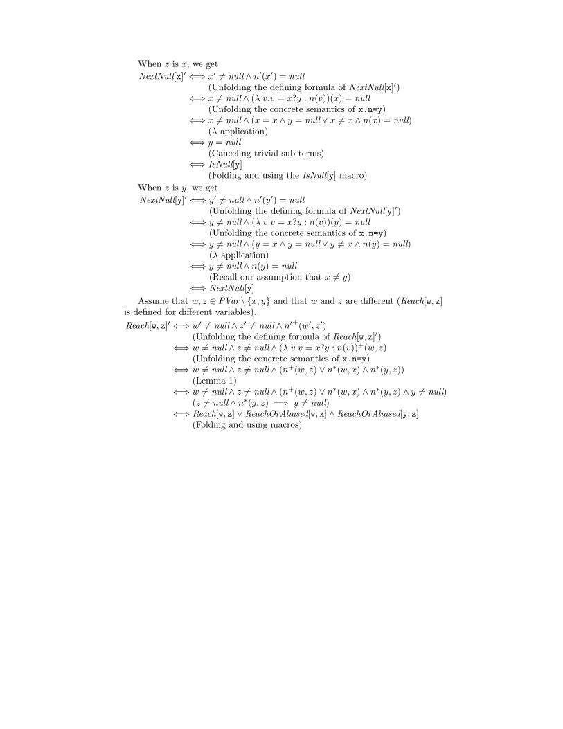
When z is x, we get

NextNull[x]′ ⇐⇒ x′ 6= null ∧ n′(x′) = null(Unfolding the defining formula of NextNull[x]′)

⇐⇒ x 6= null ∧ (λ v.v = x?y : n(v))(x) = null(Unfolding the concrete semantics of x.n=y)

⇐⇒ x 6= null ∧ (x = x ∧ y = null ∨ x 6= x ∧ n(x) = null)(λ application)

⇐⇒ y = null(Canceling trivial sub-terms)

⇐⇒ IsNull[y](Folding and using the IsNull[y] macro)

When z is y, we get

NextNull[y]′ ⇐⇒ y′ 6= null ∧ n′(y′) = null(Unfolding the defining formula of NextNull[y]′)

⇐⇒ y 6= null ∧ (λ v.v = x?y : n(v))(y) = null(Unfolding the concrete semantics of x.n=y)

⇐⇒ y 6= null ∧ (y = x ∧ y = null ∨ y 6= x ∧ n(y) = null)(λ application)

⇐⇒ y 6= null ∧ n(y) = null(Recall our assumption that x 6= y)

⇐⇒ NextNull[y]

Assume that w, z ∈ PVar \ {x, y} and that w and z are different (Reach[w, z]is defined for different variables).

Reach[w, z]′ ⇐⇒ w′ 6= null ∧ z′ 6= null ∧ n′+(w′, z′)(Unfolding the defining formula of Reach[w, z]′)

⇐⇒ w 6= null ∧ z 6= null ∧ (λ v.v = x?y : n(v))+(w, z)(Unfolding the concrete semantics of x.n=y)

⇐⇒ w 6= null ∧ z 6= null ∧ (n+(w, z) ∨ n∗(w, x) ∧ n∗(y, z))(Lemma 1)

⇐⇒ w 6= null ∧ z 6= null ∧ (n+(w, z) ∨ n∗(w, x) ∧ n∗(y, z) ∧ y 6= null)(z 6= null ∧ n∗(y, z) =⇒ y 6= null)

⇐⇒ Reach[w, z] ∨ ReachOrAliased[w, x] ∧ ReachOrAliased[y, z](Folding and using macros)

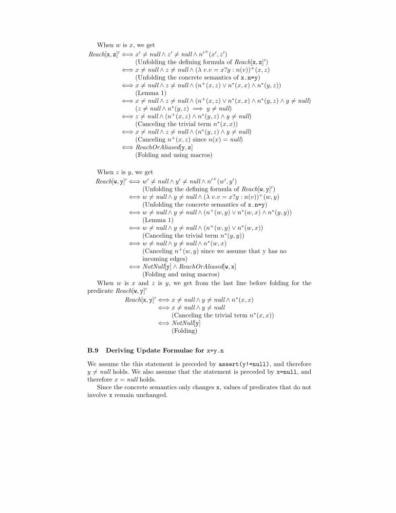
When w is x, we get

Reach[x, z]′ ⇐⇒ x′ 6= null ∧ z′ 6= null ∧ n′+(x′, z′)(Unfolding the defining formula of Reach[x, z]′)

⇐⇒ x 6= null ∧ z 6= null ∧ (λ v.v = x?y : n(v))+(x, z)(Unfolding the concrete semantics of x.n=y)

⇐⇒ x 6= null ∧ z 6= null ∧ (n+(x, z) ∨ n∗(x, x) ∧ n∗(y, z))(Lemma 1)

⇐⇒ x 6= null ∧ z 6= null ∧ (n+(x, z) ∨ n∗(x, x) ∧ n∗(y, z) ∧ y 6= null)(z 6= null ∧ n∗(y, z) =⇒ y 6= null)

⇐⇒ z 6= null ∧ (n+(x, z) ∧ n∗(y, z) ∧ y 6= null)(Canceling the trivial term n∗(x, x))

⇐⇒ x 6= null ∧ z 6= null ∧ (n∗(y, z) ∧ y 6= null)(Canceling n+(x, z) since n(x) = null)

⇐⇒ ReachOrAliased[y, z](Folding and using macros)

When z is y, we get

Reach[w, y]′ ⇐⇒ w′ 6= null ∧ y′ 6= null ∧ n′+(w′, y′)(Unfolding the defining formula of Reach[w, y]′)

⇐⇒ w 6= null ∧ y 6= null ∧ (λ v.v = x?y : n(v))+(w, y)(Unfolding the concrete semantics of x.n=y)

⇐⇒ w 6= null ∧ y 6= null ∧ (n+(w, y) ∨ n∗(w, x) ∧ n∗(y, y))(Lemma 1)

⇐⇒ w 6= null ∧ y 6= null ∧ (n+(w, y) ∨ n∗(w, x))(Canceling the trivial term n∗(y, y))

⇐⇒ w 6= null ∧ y 6= null ∧ n∗(w, x)(Canceling n+(w, y) since we assume that y has noincoming edges)

⇐⇒ NotNull[y] ∧ ReachOrAliased[w, x](Folding and using macros)

When w is x and z is y, we get from the last line before folding for thepredicate Reach[w, y]′

Reach[x, y]′ ⇐⇒ x 6= null ∧ y 6= null ∧ n∗(x, x)⇐⇒ x 6= null ∧ y 6= null

(Canceling the trivial term n∗(x, x))⇐⇒ NotNull[y]

(Folding)

B.9 Deriving Update Formulae for x=y.n

We assume the this statement is preceded by assert(y!=null), and thereforey 6= null holds. We also assume that the statement is preceded by x=null, andtherefore x = null holds.

Since the concrete semantics only changes x, values of predicates that do notinvolve x remain unchanged.

Lemma 3. When y 6= null holds the following equivalence also holds:

n(y) 6= null ⇐⇒ ¬NextNull[y] .

Proof. The following equivalence-preserving transformations proves the claim:

n(y) 6= null ⇐⇒¬(n(y) = null) ⇐⇒¬(y 6= null ∧ n(y) = null) ⇐⇒¬NextNull[y] .

⊓⊔

We know that y 6= null holds for all inputs for this transformers and thus wereplace n(y) 6= null with ¬NextNull[y] in the following derivations.

NotNull[x]′ ⇐⇒ x′ 6= null(Unfolding the defining formula of NotNull[x]′)

⇐⇒ n(y) 6= null(Unfolding the concrete semantics of x=y.n)

⇐⇒ ¬NextNull[y](Lemma 3)

Assume that z ∈ PVar \ {x, y}.Aliased[x, z]′ ⇐⇒ x′ 6= null ∧ z′ 6= null ∧ x′ = z′)

(Unfolding the defining formula of Aliased[x, z]′)⇐⇒ n(y) 6= null ∧ z 6= null ∧ n(y) = z

(Unfolding the concrete semantics of x=y.n)⇐⇒ z 6= null ∧ n(y) = z

(z 6= null ∧ n(y) = z =⇒ n(y) 6= null)⇐⇒ y 6= null ∧ z 6= null ∧ n(y) = z

(We know that y 6= null holds)Next[y, z](Folding)

Since The definition of Aliased[x, z] and Aliased[z, x] is symmetric the sameupdate is used for Aliased[z, x].

Lemma 4. If u and v are elements of unshared lists such that u 6= null, v 6= null,then n(u) = n(v) ↔ u = v.

Proof. Follows from Definition 2. ⊓⊔

Assume that z ∈ PVar \ {x, y}.Next[z, x]′ ⇐⇒ z′ 6= null ∧ x′ 6= null ∧ n′(z′) = x′)

(Unfolding the defining formula of Next[z, x]′)⇐⇒ z 6= null ∧ n(y) 6= null ∧ n(z) = n(y))

(Unfolding the concrete semantics of x=y.n)⇐⇒ z 6= null ∧ y 6= null ∧ n(y) 6= null ∧ n(z) = n(y)

(We know that y 6= null holds)⇐⇒ z 6= null ∧ y 6= null ∧ n(y) 6= null ∧ z = y

(Lemma 4)¬NextNull[y] ∧ Aliased[z, y](Folding, using Lemma 3)

When z is y, we get

Next[y, x]′ ⇐⇒ y′ 6= null ∧ x′ 6= null ∧ n′(y′) = x′)(Unfolding the defining formula of Next[y, x]′)

⇐⇒ y 6= null ∧ n(y) 6= null ∧ n(y) = n(y))(Unfolding the concrete semantics of x=y.n)

⇐⇒ y 6= null ∧ n(y) 6= null(Removing n(y) = n(y))

⇐⇒ ¬NextNull[y](Folding)

Lemma 5. For acyclic lists, and two list elements y and z, such that z, y, n(y) 6=null, the following holds:

n+(n(y), z) ⇐⇒ n+(y, z) ∧ n(y) 6= z .

Proof. Assume that n+(n(y), z) holds. Then there exists the path u1, . . . , uk

such that u1 = n(y), uk = z, and k > 1. Therefore, there exists the pathy, u1, . . . , uk. Hence, n+(y, z) holds. Since all paths are acyclic, the elements iny, u1, . . . , uk are all distinct. Hence, n(y) 6= z.

Now assume that n+(y, z) ∧ n(y) 6= z holds. Then, there exists a pathu1, . . . , uk, such that u1 = y, uk = z, and k > 1. Since n(y) 6= z holds, weknow that k > 2. Therefore, there exists the path u2, . . . , uk where u2 = n(y)and the length of the path is at least 1 (i.e., k − 2 > 1). Therefore, n+(n(y), z)holds. ⊓⊔

Assume that z ∈ PVar \ {x, y}.Reach[x, z]′ ⇐⇒ x′ 6= null ∧ z′ 6= null ∧ n′+(x′, z′)

(Unfolding the defining formula of Reach[x, z]′)⇐⇒ n(y) 6= null ∧ z 6= null ∧ n+(n(y), z)

(Unfolding the concrete semantics of x=y.n)⇐⇒ n(y) 6= null ∧ z 6= null ∧ (n+(y, z) ∧ ¬n(y) = z)

(Lemma 5)¬NextNull[y] ∧ Reach[y, z] ∧ ¬Next[y, z](Folding, using Lemma 3)

Lemma 6. When all lists are acyclic, given two list elements y and z, such thatz, y, n(y) 6= null, the following holds:

n+(z, n(y)) ⇐⇒ n+(z, y) ∨ z = y .

Proof. Assume that n+(z, n(y)) holds. Then, there exists the path u1, . . . , uk

where u1 = z, uk = n(y), and k > 1. From the assumption that all lists areacyclic, we also know that uk−1 = y. Therefore, there exists a path between zand y of length greater or equal to 0. Hence, n+(z, y) ∨ z = y holds.

Assume that n+(z, y) ∨ z = y holds. Then, there exists a path of lengthgreater or equal to 0 from z to y. Therefore, there exists a path of length greaterthan 0 from z to n(y). Hence, n+(z, n(y)) holds. ⊓⊔

Assume that z ∈ PVar \ {x, y}.Reach[z, x]′ ⇐⇒ z′ 6= null ∧ x′ 6= null ∧ n′+(z′, x′)

(Unfolding the defining formula of Reach[z, x]′)⇐⇒ z 6= null ∧ n(y) 6= null ∧ n+(z, n(y))

(Unfolding the concrete semantics of x=y.n)z 6= null ∧ n(y) 6= null ∧ (n+(z, y) ∨ z = y)(Lemma 6)¬NextNull[y] ∧ ReachOrAliased[z, y](Folding, using Lemma 3 and macros)

When z is y, we get

Reach[y, x]′ ⇐⇒ y′ 6= null ∧ x′ 6= null ∧ n′+(y′, x′)(Unfolding the defining formula of Reach[y, x]′)

⇐⇒ y 6= null ∧ n(y) 6= null ∧ n+(y, n(y))(Unfolding the concrete semantics of x=y.n)y 6= null ∧ n(y) 6= null ∧ (n+(y, y) ∨ y = y)(Lemma 6)y 6= null ∧ n(y) 6= null¬NextNull[y](Folding)

Lemma 7. The condition formulae shown in Fig. 3 are mutually-exclusive, andexactly one of them is enabled.

Proof. The condition formulae are:

Case 1: NextNull[y] ,Case 2: ¬NextNull[y] ∧ NextPtByVar[y] ,Case 3: ¬NextNull[y] ∧ ReachNull[y] , andCase 4: ¬NextNull[y] ∧ ¬ReachNull[y] ∧ ¬NextPtByVar[y] .

Recall that, for the statement x=y.n to be executed, we require that y 6= nullhold, hence NotNull[y] holds for all of the cases.

The formula ReachNull[y] means that by following n links, we do not en-counter any element that is pointed-to by some variable. Therefore, ReachNull[y]implies ¬NextPtByVar[y] (which means that the next element after y is notpointed-to by any variable). Therefore, the condition formula of case 3 rewrites

to

NotNull[y] ∧ ¬NextNull[y] ∧ ReachNull[y] ∧ ¬NextPtByVar[y] .

Now it is evident from the structure of the condition formulae that they par-tition the set of concrete states since they contain complementary sub-formulae.

⊓⊔

We continue to show the derivation of the update formulae for the predicatesNextNull[x] and Next[x, z] by considering each case separately.

Case 1: the condition NextNull[y] holds. Since a statement x=y.n is pre-ceded by a statement x=null, the fact that the condition formula NotNull[y] ∧NextNull[y] holds means that n(y) = null, and thus no change occurs in theconcrete semantics. Therefore, the values of all predicates remain unchanged.

Case 2 : the condition NotNull[y] ∧ ¬NextNull[y] ∧ NextPtByVar[y]holds.

Lemma 8. Under the condition of case 2, the following holds:

n(n(y)) = null ⇐⇒∨

w∈PVar\{x,y}

Next[y, w] ∧ NextNull[w] .

Proof. We first show that the right-hand side implies the left-hand side:∨

w∈PVar\{x,y} Next[y, w] ∧ NextNull[w] =⇒(Assuming the left-hand side)∨

w∈PVar\{x,y} y 6= null ∧ w 6= null ∧ n(y) = w ∧ n(w) = null =⇒(Unfolding the definitions of the predicates)∃u : y 6= null ∧ u 6= null ∧ n(y) = u ∧ n(u) = null ⇐⇒(Applying a valid first-order logic transformation:Let c be a constant. Then φ(c) =⇒ ∃v.φ(v))∃u : n(y) = u ∧ n(u) = null ⇐⇒(Using the condition to eliminate trivial terms)n(n(y)) = null ⇐⇒(Folding by using the meaning of applying a function twice)

We now show that the left-hand side implies the right-hand side:

n(n(y)) = null ⇐⇒(Assuming the left-hand side)∃u : n(y) = u ∧ n(u) = null ⇐⇒(Unfolding the meaning of applying a function twice)∃u : n(y) = u ∧ (

∨

z∈PVar\{x,y} u = z) ∧ n(u) = null ⇐⇒(Since NextPtByVar[y] and x = null hold, u = n(y) =⇒ ∨

z∈PVar\{x,y} u = z)

∃u :∨

z∈PVar\{x,y}(n(y) = u ∧ u = z ∧ n(u) = null) ⇐⇒(Distributivity of ∨ over ∧)∃u :

∨

z∈PVar\{x,y}(n(y) = z ∧ u = z ∧ n(z) = null) =⇒(Using u = z to substitute u by z)∃u :

∨

z∈PVar\{x,y}(n(y) = z ∧ n(z) = null) ⇐⇒(Removing a conjunct weakens the formula)∨

z∈PVar\{x,y}(n(y) = z ∧ n(z) = null) ⇐⇒(Removing the quantifier with empty binding)∨

z∈PVar\{x,y}(Next[y, z] ∧ NextNull[z])

⊓⊔

NextNull[x]′ ⇐⇒ x′ 6= null ∧ n′(x′) = null(Unfolding the defining formula of NextNull[x]′)n(y) 6= null ∧ n(n(y)) = null(Unfolding the concrete semantics of x=y.n)∨

w∈PVar\{x,y} Next[y, w] ∧ NextNull[w]

(Lemma 8)

Lemma 9. Under the condition of case 2, the following holds for any z ∈ PVar\y:

n(n(y)) = z ⇐⇒∨

w∈PVar\{x,y}

Next[y, w] ∧ Next[w, z] .

Proof. We first show that the right-hand side implies the left-hand side:∨

w∈PVar\{x,y} Next[y, w] ∧ Next[w, z] =⇒(Assuming the left-hand side)∨

w∈PVar\{x,y} y 6= null ∧ w 6= null ∧ n(y) = w ∧ n(w) = z =⇒(Unfolding the definitions of the predicates)∃u : y 6= null ∧ u 6= null ∧ n(y) = u ∧ n(u) = z ⇐⇒(Applying a valid first-order logic transformation:Let c be a constant. Then φ(c) =⇒ ∃v.φ(v))∃u : n(y) = u ∧ n(u) = z ⇐⇒(Using the condition to eliminate trivial terms)n(n(y)) = z(Folding by using the meaning of applying a function twice)

We now show that the left-hand side implies the right-hand side:

n(n(y)) = z ⇐⇒(Assuming the left-hand side)∃u : n(y) = u ∧ n(u) = z ⇐⇒(Unfolding the meaning of applying a function twice)∃u : n(y) = u ∧ (

∨

w∈PVar\{x,y} u = w) ∧ n(u) = z ⇐⇒(Since NextPtByVar[y], x = null, and n(u) 6= null hold,u = n(y) =⇒ ∨

w∈PVar\{x,y} u = w)

∃u :∨

w∈PVar\{x,y}(n(y) = u ∧ u = w ∧ n(u) = z) ⇐⇒(Distributivity of ∨ over ∧)∃u :

∨

w∈PVar\{x,y}(n(y) = w ∧ u = w ∧ n(w) = z) =⇒(Using u = w to substitute u by w)∃u :

∨

w∈PVar\{x,y}(n(y) = w ∧ n(w) = z) ⇐⇒(Removing a conjunct weakens the formula)∨

w∈PVar\{x,y}(n(y) = w ∧ n(w) = z) ⇐⇒(Removing the quantifier with empty binding)∨

w∈PVar\{x,y}(Next[y, w] ∧ Next[w, z])

⊓⊔

Assume that z ∈ PVar \ {x, y}.Next[x, z]′ ⇐⇒ x′ 6= null ∧ z′ 6= null ∧ n′(x′) = z′

(Unfolding the defining formula of Next[x, z]′)⇐⇒ n(y) 6= null ∧ z 6= null ∧ n(n(y)) = z

(Unfolding the concrete semantics of x=y.n)∨

w∈PVar\{x,y} Next[y, w] ∧ Next[w, z]

(Lemma 9)

Case 3 : NotNull[y]∧¬NextNull[y]∧ReachNull[y] holds. The next lemmashows that there are concrete states that are indistinguishable by the abstractionbut are distinguishable by the focus formula NextNextNull[y] ≡ n(n(y)) = null.

Lemma 10. When the condition of case 3 holds, the predicate NextNextNull[y]is a focus predicate.

In other words, let σ0 be a concrete state that satisfies the condition formula.Then, there exist two concrete states (containing only acyclic unshared lists)σ1, σ2 such that σ1 |= NextNextNull[y] and σ2 |= ¬NextNextNull[y], and α(σ0) =α(σ1) = α(σ2).

Proof. We show that we can modify σ0 to obtain two concrete states, σ1 andσ2, such that α(σ0) = α(σ1) = α(σ2), and σ1 |= NextNextNull[y] and σ2 |=¬NextNextNull[y].

From the fact that σ0 satisfies the condition, we have that σ0 contains a pathu1, . . . , uk such that u1 = y, uk = null (since y 6= null holds and there exists apath from every non-null variable to null, k > 1 (since ¬NextNull[y] holds), andu2, . . . , uk−1 are not pointed-to by any variable (since ReachNull[y] holds).

To obtain σ1, we replace the path u1, . . . , uk with the path u1, u2, uk, byremoving the elements u3, . . . , uk−1 from the heap and adjusting the n linksaccordingly. Thus, n(n(y)) = null in σ1, i.e., σ1 |= NextNextNull[y].

To obtain σ2, we replace the path u1, . . . , uk with the path u1, u′, u2, uk where

u′ is a new element added to the heap between u1 and u2. Since k > 1 in σ0, wehave that u2 6= null. Thus, n(n(y)) 6= null in σ2, i.e., σ2 |= ¬NextNextNull[y].

Intuitively, to obtain σ1 and σ2, we have changed σ0 by modifying the lengthof the path from y to null, which used to be greater than 1. However, the ab-straction we use does not distinguish between lengths of lists greater than 1, andthus we get 3 concrete states that are equivalent under the abstraction.

Now, since in σ0, none of the elements u2, . . . , uk−1 are pointed-to by vari-ables, every logical constant z representing a variable z, evaluates to the same ele-ment in σ0, σ1, and σ2. Therefore, [[NotNull[z]]]σ0 = [[NotNull[z]]]σ1 = [[NotNull[z]]]σ2 ,for every z ∈ PVar. As well, [[Aliased[z, w]]]σ0 = [[Aliased[z, w]]]σ1 = [[Aliased[z, w]]]σ2

for every z, w ∈ PVar.Let z be in PVar such that z = null in σ0. Then, z = null in σ1 and

σ2. Therefore, [[NextNull[z]]]σ0 = [[NextNull[z]]]σ1 = [[NextNull[z]]]σ2 = 0. Thisalso means that for every w ∈ PVar, we have [[Next[z, w]]]σ0 = [[Next[z, w]]]σ1 =[[Next[z, w]]]σ2 = 0, [[Next[w, z]]]σ0 = [[Next[w, z]]]σ1 = [[Next[w, z]]]σ2 = 0, [[Reach[w, z]]]σ0 =[[Reach[w, z]]]σ1 = [[Reach[w, z]]]σ2 = 0, and [[Reach[z, w]]]σ0 = [[Reach[z, w]]]σ1 =[[Reach[z, w]]]σ2 = 0.

We now have to show that the equality holds for predicates of the formNextNull[z], Next[z, w], and Reach[z, w] such that both z and w are differentfrom null in σ0.

The only element pointed-to by a variable for which the outgoing edge haschanged is the one pointed-to by y. Therefore, for every z ∈ PVar \ {y} suchthat y 6= z, [[n(z) = null]]σ0 = [[n(z) = null]]σ1 = [[n(z) = null]]σ2 . Hence,[[NextNull[z]]]σ0 = [[NextNull[z]]]σ1 = [[NextNull[z]]]σ2 .

For every z ∈ PVar \ {y} such that y = z, we have [[NextNull[z]]]σ0 = 0(since the statement is preceded by assert(y!=null)). In σ1 and σ2, we haven(z) = u1. Thus, [[NextNull[z]]]σ0 = [[NextNull[z]]]σ1 = [[NextNull[z]]]σ2 = 0.

Let w and z be two variables in PVar such that w and z are distinct andboth are different from null. The path between w and z is the same in σ0 asin σ1 and σ2. Therefore, [[Reach[z, w]]]σ0 = [[Reach[z, w]]]σ1 = [[Reach[z, w]]]σ2 = 0,and [[Next[z, w]]]σ0 = [[Next[z, w]]]σ1 = [[Next[z, w]]]σ2 = 0. ⊓⊔

NextNull[x]′ ⇐⇒ x′ 6= null ∧ n′(x′) = null(Unfolding the defining formula of NextNull[x]′)n(y) 6= null ∧ n(n(y)) = null(Unfolding the concrete semantics of x=y.n)NextNextNull[y](Folding)

Assume that z ∈ PVar \ {x, y}.Next[x, z]′ ⇐⇒ x′ 6= null ∧ z′ 6= null ∧ n′(x′) = z′

(Unfolding the defining formula of Next[x, z]′)⇐⇒ x 6= null ∧ z 6= null ∧ n(n(y)) = z

(Unfolding the concrete semantics of x=y.n)⇐⇒ 0

(Since y 6= nullz 6= null ∧ n(n(y)) = z =⇒ Reach[y, z] =⇒¬ReachNull[y], yet we have that ReachNull[y] holdsin the condition.)

Case 4 : the condition NotNull[y] ∧ ¬NextNull[y] ∧ ¬ReachNull[y] ∧

¬NextPtByVar[y] holds.

Lemma 11. Under the condition of case 4, the predicate NextNextPtByVar[y]is a focus predicate.

In other words, let σ0 be a concrete state that satisfies the condition formula.Then, there exist two concrete states (containing only acyclic unshared lists)σ1, σ2 such that σ1 |= NextNextNull[y] and σ2 |= ¬NextNextNull[y], and α(σ0) =α(σ1) = α(σ2).

Proof. We show that we can modify σ0 to obtain two concrete states, σ1 andσ2, such that α(σ0) = α(σ1) = α(σ2), and σ1 |= NextNextPtByVar[y] and σ2 |=¬NextNextPtByVar[y].

From the fact that σ0 satisfies the condition, we have that σ0 contains apath u1, . . . , uk such that u1 = y, uk is pointed-to by some variable (since¬ReachNull[y] holds), and u2, . . . , uk−1 are not pointed-to by any variable, andk > 1 (since ¬NextPtByVar[y] holds).

To obtain σ1, we replace the path u1, . . . , uk with the path u1, u2, uk, byremoving the elements u3, . . . , uk−1 from the heap and adjusting the n linksaccordingly. Thus, n(n(y)) = uk in σ1, i.e., σ1 |= NextNextPtByVar[y].

To obtain σ2, we replace the path u1, . . . , uk with the path u1, u′, u2, uk

where u′ is a new element added to the heap between u1 and u2. Since neitherof u′ and u2 are pointed-to by a variable, σ2 |= ¬NextNextPtByVar[y].

Intuitively, to obtain σ1 and σ2, we have changed σ0 by modifying the lengthof the path from y to uk, which used to be greater than 1. However, the abstrac-tion we use does not distinguish between lengths of lists greater than 1, and thuswe get 3 concrete states that are equivalent under the abstraction.

Now, since in σ0, none of the elements u2, . . . , uk−1 were are pointed-to byvariables, every logical constant z representing a variable z, evaluates to thesame element in σ0, σ1, and σ2. Therefore, [[NotNull[z]]]σ0 = [[NotNull[z]]]σ1 =[[NotNull[z]]]σ2 , for every z ∈ PVar. As well, [[Aliased[z, w]]]σ0 = [[Aliased[z, w]]]σ1 =[[Aliased[z, w]]]σ2 for every z, w ∈ PVar.

Let z be in PVar such that z = null in σ0. Then, z = null in σ1 andσ2. Therefore, [[NextNull[z]]]σ0 = [[NextNull[z]]]σ1 = [[NextNull[z]]]σ2 = 0. Thisalso means that for every w ∈ PVar, we have [[Next[z, w]]]σ0 = [[Next[z, w]]]σ1 =

[[Next[z, w]]]σ2 = 0, [[Next[w, z]]]σ0 = [[Next[w, z]]]σ1 = [[Next[w, z]]]σ2 = 0, [[Reach[w, z]]]σ0 =[[Reach[w, z]]]σ1 = [[Reach[w, z]]]σ2 = 0, and [[Reach[z, w]]]σ0 = [[Reach[z, w]]]σ1 =[[Reach[z, w]]]σ2 = 0.

We now have to show that the equality holds for predicates of the formNextNull[z], Next[z, w], and Reach[z, w] such that both z and w are differentfrom null in σ0.

The only element pointed-to by a variable for which the outgoing edge haschanged is the one pointed-to by y. Therefore, for every z ∈ PVar \ {y} suchthat y 6= z, [[n(z) = null]]σ0 = [[n(z) = null]]σ1 = [[n(z) = null]]σ2 . Hence,[[NextNull[z]]]σ0 = [[NextNull[z]]]σ1 = [[NextNull[z]]]σ2 .

For every z ∈ PVar \ {y} such that y = z, we have [[NextNull[z]]]σ0 = 0(since the statement is preceded by assert(y!=null)). In σ1 and σ2, we haven(z) = u1. Thus, [[NextNull[z]]]σ0 = [[NextNull[z]]]σ1 = [[NextNull[z]]]σ2 = 0.

Let w and z be two variables in PVar such that w and z are distinct andboth are different from null. If any of w and z are not on the same list as yin σ0 then [[Next[w, z]]]σ0 = [[Next[w, z]]]σ1 = [[Next[w, z]]]σ2 and [[Reach[w, z]]]σ0 =[[Reach[w, z]]]σ1 = [[Reach[w, z]]]σ2 , since only the list containing y is possibly dif-ferent in these states. Assume that, in σ0, w and z are on the list contain-ing y in, and without loss of generality let z be reachable from w. If the pathbetween w and z does not contain the path u0, . . . , uk then it remains thesame in all three states, and thus [[Next[w, z]]]σ0 = [[Next[w, z]]]σ1 = [[Next[w, z]]]σ2

and [[Reach[w, z]]]σ0 = [[Reach[w, z]]]σ1 = [[Reach[w, z]]]σ2 . Assume that, in σ0, thepath from w to z is v1, . . . , vg, u1, . . . , uk, h1, . . . , jp where k > 1, g ≥ 1, andp ≥ 1. Then, in σ1 the path from w to z is v1, . . . , vg, u1, u2, uk, h1, . . . , jpand in σ1 the path from w to z is v1, . . . , vg, u1, u

′, . . . , uk, h1, . . . , jp. There-fore, [[Next[w, z]]]σ0 = [[Next[w, z]]]σ1 = [[Next[w, z]]]σ2 = 0 and [[Reach[w, z]]]σ0 =[[Reach[w, z]]]σ1 = [[Reach[w, z]]]σ2 . ⊓⊔

Lemma 12. Under the condition of case 3, n(n(y)) 6= null holds:

Proof. By Contradiction. Assume that the condition of case 3 and n(n(y)) = nullhold simultaneously.

Since n(n(y)) = null holds, we have that nj(y) = null for every j ≥ 2.Therefore, for every w ∈ PVar, if w 6= null then n+(y, w) holds when n(y) = wholds.

Now, for every w ∈ PVar, we have

Reach[y, w] ⇐⇒y 6= null ∧ w 6= null ∧ n+(y, w) ⇐⇒(Unfolding the predicate definition)y 6= null ∧ w 6= null ∧ n(y) = w ⇐⇒(Since w 6= null and nj(y) = null for j ≥ 2)Next[y, w] =⇒(Folding)∨

z∈PVar\{y} Next[y, z] ⇐⇒(Weakening)NextPtByVar[y] ⇐⇒(Folding)0(Since, by the condition of case 3, ¬NextPtByVar[y] holds)

We now have that ¬Reach[y, q] holds for every w ∈ PVar, i.e.,∧

w∈PVar\y ¬Reach[y, w]

holds. Therefore, ReachNull[y] holds. However, by the condition of case 3, ¬ReachNull[y]also holds. We have arrived to a contradiction. ⊓⊔

NextNull[x]′ ⇐⇒ x′ 6= null ∧ n′(x′) = null(Unfolding the defining formula of NextNull[x]′)n(y) 6= null ∧ n(n(y)) = null(Unfolding the concrete semantics of x=y.n)0(Lemma 12)

Lemma 13. Under the condition of case 3, the following holds for every z ∈PVar \ {y}:

z 6= null ∧ n(n(y)) = z ⇐⇒ NextNextPtByVar[y] ∧ ReachFirst[y, z] .

Proof. Assume that z 6= null∧n(n(y)) = z holds. This implies that∨

w∈PVar\{y} w 6=null ∧ n(n(y)) = w holds. Hence, NextNextPtByVar[y] holds.

We now show that ReachFirst[y, z] also holds. The following calculation showsthat Reach[y, z] holds.

z 6= null ∧ n(n(y)) = z =⇒z 6= null ∧ n+(y, z) ⇐⇒y 6= null ∧ z 6= null ∧ n+(y, z) ⇐⇒(By the condition of case 4)Reach[y, z](Folding)

Now assume that Reach[y, w] for w ∈ PVar \ {y}. This means that w 6= nulland there exists the unique path u1, . . . , uk such that u1 = y and uk = w. Bythe condition of case 4, we have that ¬NextPtByVar[y] holds. Therefore, k ≥ 2.Since z 6= null ∧ n(n(y)) = z also holds and n is deterministic, we have thatu2 = z and therefore, n∗(z, w) holds. This shows that ReachFirst[y, z] holds.

Now assume that NextNextPtByVar[y]∧ReachFirst[y, z] holds. From the firstconjunct, we have that there exists w ∈ PVar\{y} for which w 6= null∧n(n(y)) =w holds. Choose such a w without loss of generality.

Since ReachFirst[y, z] holds, we have that n+(y, z) holds, i.e., there exists theunique path u1, . . . , uk such that u1 = y, uk = z, and k ≥ 1. From the conjunct¬NextPtByVar[y] in the condition, we know that k ≥ 2.

Also, from the fact ReachFirst[y, z] and n+(y, w) hold, we have that n∗(z, w)also holds. However, w = u2, and therefore z = w. Substituting w with z, weget that z 6= null ∧ n(n(y)) = z holds. ⊓⊔

Assume that z ∈ PVar \ {x, y}.Next[x, z]′ ⇐⇒ x′ 6= null ∧ z′ 6= null ∧ n′(x′) = z′

(Unfolding the defining formula of Next[x, z]′)⇐⇒ x 6= null ∧ z 6= null ∧ n(n(y)) = z

(Unfolding the concrete semantics of x=y.n)NextNextPtByVar[y] ∧ ReachFirst[y, z](Lemma 13)