Embed Size (px)
Citation preview
Light in Strongly Scattering
and Amplifying Random Media
Academisch Proefschrift
ter verkrijging van de graad van doctor
aan de Universiteit van Amsterdam,
op gezag van de Rector Magnificus
prof.dr P.W.M. de Meijer
ten overstaan van een door het
college van dekanen ingestelde commissie
in het openbaar te verdedigen
in de Aula der Universiteit
op dinsdag 21 november 1995 te 12:00 uur
door
Diederik Sybolt Wiersma
geboren te Utrecht
Promotor: prof. dr. A. LagendijkCopromotor: dr. M.P. van Albada
Overige leden commissie:prof. dr. A. Aspectprof. dr. D. Frenkelprof. dr. K.J.F. Gaemersprof. dr. J.F. v.d. Veenprof. dr. J.T.M. Walraven
Faculteit der Wiskunde, Informatica, Natuurkunde en Sterrenkunde
The work described in this thesis is part of the research programof the ‘Stichting Fundamenteel Onderzoek van de Materie’
(Foundation for Fundamental Research on Matter)and was made possible by financial support from the
‘Nederlandse Organisatie voor Wetenschappelijk Onderzoek’(Netherlands Organization for the Advancement of Research).
The research has been performed at the
FOM-Institute for Atomic and Molecular PhysicsKruislaan 407
1098 SJ Amsterdam
where a number of copies of this thesis is available.
Look, the sun was sleeping in the clouds this morningup those mountains you can feel the glowchildren playing in the valley, flyingin the winds they know that meet belowas their heart was beating fast this morning.

Contents
1 Introduction 91.1 Light scattering . . . . . . . . . . . . . . . . . . . . . . . . . 9
1.1.1 Single scattering . . . . . . . . . . . . . . . . . . . . 91.1.2 Multiple scattering . . . . . . . . . . . . . . . . . . . 121.1.3 Light versus electrons . . . . . . . . . . . . . . . . . 13
1.2 Lasers . . . . . . . . . . . . . . . . . . . . . . . . . . . . . . 161.3 This thesis . . . . . . . . . . . . . . . . . . . . . . . . . . . . 18
2 Multiple scattering theory 212.1 Introduction . . . . . . . . . . . . . . . . . . . . . . . . . . . 212.2 Diffusion of light . . . . . . . . . . . . . . . . . . . . . . . . 21
2.2.1 Stationary solution for a slab . . . . . . . . . . . . . 222.3 Multiple scattering of waves . . . . . . . . . . . . . . . . . . 24
2.3.1 Electric field . . . . . . . . . . . . . . . . . . . . . . 242.3.2 Intensity . . . . . . . . . . . . . . . . . . . . . . . . . 29
2.4 Backscattered intensity . . . . . . . . . . . . . . . . . . . . . 312.5 Coherent backscattering . . . . . . . . . . . . . . . . . . . . 36
2.5.1 Properties of the backscattering cone . . . . . . . . . 37
3 An accurate technique to record coherent backscattering 413.1 Introduction . . . . . . . . . . . . . . . . . . . . . . . . . . . 41
3.1.1 Principle of previous setups . . . . . . . . . . . . . . 423.2 Experimental configuration . . . . . . . . . . . . . . . . . . 43
3.2.1 Principle of the setup . . . . . . . . . . . . . . . . . 433.2.2 Polarization . . . . . . . . . . . . . . . . . . . . . . . 453.2.3 Angular resolution and scanning range . . . . . . . . 463.2.4 Elimination of important artifacts . . . . . . . . . . 473.2.5 Response of the setup . . . . . . . . . . . . . . . . . 48
3.3 Results . . . . . . . . . . . . . . . . . . . . . . . . . . . . . . 493.3.1 Enhancement factor . . . . . . . . . . . . . . . . . . 49
5
6 Contents
3.3.2 The shape of the backscattering cone . . . . . . . . . 51
4 Experimental evidence for recurrent multiple scattering 574.1 Introduction . . . . . . . . . . . . . . . . . . . . . . . . . . . 574.2 Experimental procedure . . . . . . . . . . . . . . . . . . . . 59
4.2.1 Preparation of strongly scattering samples . . . . . . 594.2.2 Enhancement factor in coherent backscattering . . . 604.2.3 Determination of the mean free path . . . . . . . . . 62
4.3 Results . . . . . . . . . . . . . . . . . . . . . . . . . . . . . . 634.3.1 Enhancement factor versus mean free path . . . . . 63
4.4 Interpretation . . . . . . . . . . . . . . . . . . . . . . . . . . 664.5 Theory . . . . . . . . . . . . . . . . . . . . . . . . . . . . . . 66
4.5.1 Two particle recurrent scattering . . . . . . . . . . . 70
5 Amplifying random media 775.1 Introduction . . . . . . . . . . . . . . . . . . . . . . . . . . . 77
5.1.1 Relevant length scales . . . . . . . . . . . . . . . . . 785.2 Realizing disordered media with gain . . . . . . . . . . . . . 79
5.2.1 Choice of the laser material . . . . . . . . . . . . . . 795.2.2 Optical excitation . . . . . . . . . . . . . . . . . . . 805.2.3 Experimentally realized gain levels . . . . . . . . . . 84
5.3 Calculations on diffusion with gain . . . . . . . . . . . . . . 855.3.1 Discretization . . . . . . . . . . . . . . . . . . . . . . 895.3.2 Backscattered flux . . . . . . . . . . . . . . . . . . . 905.3.3 Spatial profile of the excitation level . . . . . . . . . 925.3.4 Pulsed amplified spontaneous emission . . . . . . . . 94
5.4 Random lasers . . . . . . . . . . . . . . . . . . . . . . . . . 98
6 Experiments on random media with gain 1056.1 Introduction . . . . . . . . . . . . . . . . . . . . . . . . . . . 1056.2 Laser speckle . . . . . . . . . . . . . . . . . . . . . . . . . . 106
6.2.1 Experimental configuration and results . . . . . . . . 1076.2.2 Interpretation . . . . . . . . . . . . . . . . . . . . . . 108
6.3 Coherent backscattering . . . . . . . . . . . . . . . . . . . . 1106.3.1 Samples . . . . . . . . . . . . . . . . . . . . . . . . . 1106.3.2 Setup . . . . . . . . . . . . . . . . . . . . . . . . . . 1106.3.3 Results . . . . . . . . . . . . . . . . . . . . . . . . . 1136.3.4 Interpretation . . . . . . . . . . . . . . . . . . . . . . 1136.3.5 Theory . . . . . . . . . . . . . . . . . . . . . . . . . 117
6.4 Discussion . . . . . . . . . . . . . . . . . . . . . . . . . . . . 124

A List of symbols 127
B Feynman notation 129
Summary 133
Samenvatting 135
Dankwoord 139

8 Contents
Chapter 1
Introduction
1.1 Light scattering
An object is visible because it scatters, reflects or absorbs light. In thefirst two cases an interaction takes place between light waves and matter inwhich the propagation direction of the waves is changed. In this interactionthe light waves do not lose energy. Reflection is very similar to scattering:one can describe reflection as a special case of scattering in which incomingand outgoing angle are equal. Apart from being scattered, light can also beabsorbed by an object. In that case, the object dissipates electromagneticenergy. An object that scatters equally efficient at all wavelengths and doesnot absorb, looks white. An object that absorbs strongly at all wavelengths,looks black. The color of an object can arise both from a wavelength-dependent scattering efficiency or a wavelength-dependent absorption.
1.1.1 Single scattering
The scattering properties of a single small particle (e.g. a water droplet), arecomplicated. An incoming (‘applied’) electromagnetic field on the particleinduces in the particle an electric polarization. This polarization generatesa new electromagnetic field in and around the particle. This new total elec-tromagnetic field influences again the polarization of the particle, etc. Thetotal outgoing electromagnetic field is the result of a complicated recursiveprocess.
For particles which are very small compared to the wavelength of thelight, the angular dependence of the scattered intensity is relatively simple.In this regime the light is scattered completely isotropically for a polariza-tion perpendicular to the plane of scattering, and the scattered intensity
9
10 Introduction
0.0 1.0 2.0 3.00.0
0.5
1.0
perpendicular pol.
parallel pol.
norm
aliz
ed in
tens
ity
scattering angle (rad)
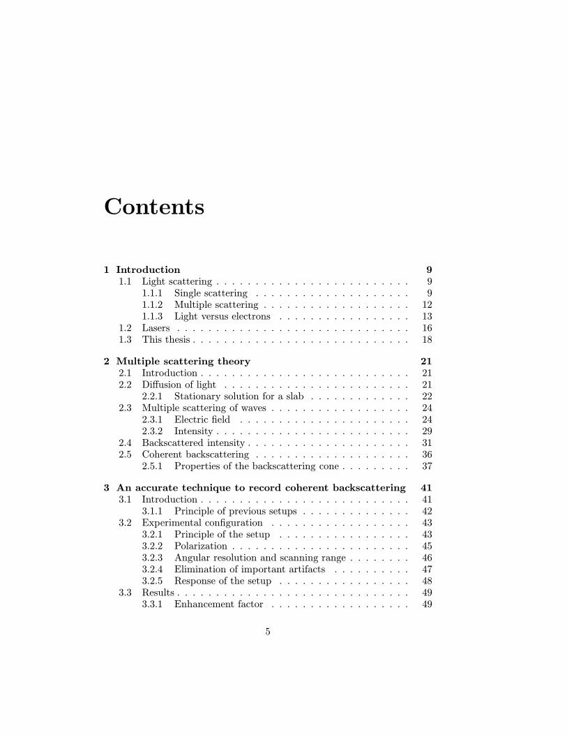
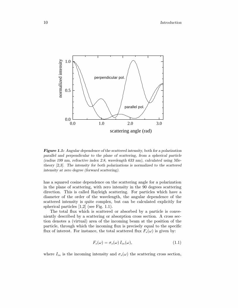
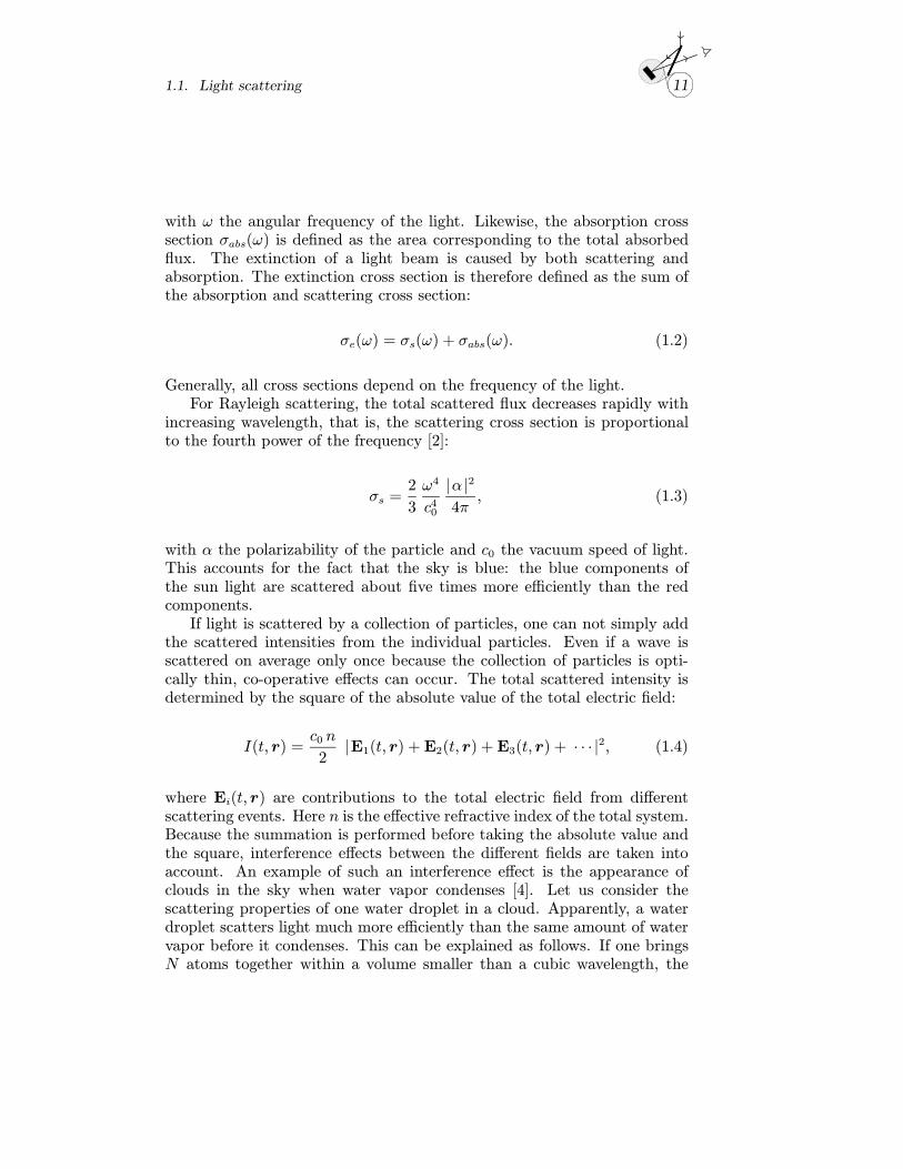
Figure 1.1: Angular dependence of the scattered intensity, both for a polarization
parallel and perpendicular to the plane of scattering, from a spherical particle
(radius 199 nm, refractive index 2.8, wavelength 633 nm), calculated using Mie-
theory [2,3]. The intensity for both polarizations is normalized to the scattered
intensity at zero degree (forward scattering).
has a squared cosine dependence on the scattering angle for a polarizationin the plane of scattering, with zero intensity in the 90 degrees scatteringdirection. This is called Rayleigh scattering. For particles which have adiameter of the order of the wavelength, the angular dependence of thescattered intensity is quite complex, but can be calculated explicitly forspherical particles [1,2] (see Fig. 1.1).
The total flux which is scattered or absorbed by a particle is conve-niently described by a scattering or absorption cross section. A cross sec-tion denotes a (virtual) area of the incoming beam at the position of theparticle, through which the incoming flux is precisely equal to the specificflux of interest. For instance, the total scattered flux Fs(ω) is given by:
Fs(ω) = σs(ω) Iin(ω), (1.1)
where Iin is the incoming intensity and σs(ω) the scattering cross section,
1.1. Light scattering 11
with ω the angular frequency of the light. Likewise, the absorption crosssection σabs(ω) is defined as the area corresponding to the total absorbedflux. The extinction of a light beam is caused by both scattering andabsorption. The extinction cross section is therefore defined as the sum ofthe absorption and scattering cross section:
σe(ω) = σs(ω) + σabs(ω). (1.2)
Generally, all cross sections depend on the frequency of the light.For Rayleigh scattering, the total scattered flux decreases rapidly with
increasing wavelength, that is, the scattering cross section is proportionalto the fourth power of the frequency [2]:
σs =2
3
ω4
c40
|α |2
4π, (1.3)
with α the polarizability of the particle and c0 the vacuum speed of light.This accounts for the fact that the sky is blue: the blue components ofthe sun light are scattered about five times more efficiently than the redcomponents.
If light is scattered by a collection of particles, one can not simply addthe scattered intensities from the individual particles. Even if a wave isscattered on average only once because the collection of particles is opti-cally thin, co-operative effects can occur. The total scattered intensity isdetermined by the square of the absolute value of the total electric field:
I(t, r) =c0 n
2|E1(t, r) + E2(t, r) + E3(t, r) + · · · |
2, (1.4)
where Ei(t, r) are contributions to the total electric field from differentscattering events. Here n is the effective refractive index of the total system.Because the summation is performed before taking the absolute value andthe square, interference effects between the different fields are taken intoaccount. An example of such an interference effect is the appearance ofclouds in the sky when water vapor condenses [4]. Let us consider thescattering properties of one water droplet in a cloud. Apparently, a waterdroplet scatters light much more efficiently than the same amount of watervapor before it condenses. This can be explained as follows. If one bringsN atoms together within a volume smaller than a cubic wavelength, the
12 Introduction
scattered fields of these atoms will all be in phase. The resulting scatteredintensity will therefore by N2 and not N times the scattered intensity ofone atom. This is an example of a collective effect of the scatterers (atoms)in the water droplet.
1.1.2 Multiple scattering
In the above example we considered the scattering by one water droplet.We call this single scattering. If we consider the scattering properties ofan (optically thick) cloud, we are dealing with multiple light scattering. Inthis multiple scattering regime, light is often assumed to propagate diffu-sively. Interference effects are assumed to be scrambled, due to the manyrandom scattering events, and the position and time-dependent intensity isdescribed by a diffusion equation.
In some cases, interference in a disordered medium can not be neglected,even for very high orders of scattering. An example is the interference be-tween waves that have propagated along the same path but in the oppositedirections. Because these waves have travelled over exactly the same dis-tance, their original phase relation is conserved, even if the path is formedby a very large number of scattering events. If the waves were originallyin phase, they will interfere constructively when they meet again. Thiseffect leads to for instance coherent backscattering, which is a general phe-nomenon for waves that are backscattered from a random medium. Dueto constructive interference between waves that have propagated along thesame path in the opposite direction, the backscattered intensity in the exactbackscattering direction is twice as high as in other directions. Coherentbackscattering is explained in detail in the next chapter. It is an exam-ple of an interference effect for light that is scattered (theoretically up toinfinitely) many times.
An important concept in multiple scattering theory is the mean freepath. A mean free path is a characteristic length scale describing the scat-tering process. For instance, the scattering mean free path is defined as theaverage distance between two successive scattering events. For a randomdistribution of small particles, any mean free path × can in principle bewritten in terms of a cross section σ×:
× =1
nσ×, (1.5)
with n the density of the scattering particles. For instance, the scatteringmean free path s is given by: s = (nσs)
−1.
1.1. Light scattering 13
The transport mean free path t is defined as the average distance thelight travels in the sample before its propagation direction is randomized.For isotropic scattering, t is equal to s. For anisotropic scattering, thetransport mean free path is given by:
t =1
1− 〈cos θ〉
1
nσs, (1.6)
where 〈cos θ〉 is the average cosine of the scattering angle for each scatteringevent. The cross section corresponding to the transport mean free path iscalled the cross section for radiation pressure σt, which describes the averagemomentum transfer to the scatterer. So for the transport mean free pathwe can write: t = (nσt)
−1. Because the transport mean free path is oftenthe relevant length scale to describe the propagation of light in disorderedsystems, we will drop the index t and just use to denote the transportmean free path.
The characteristic length scales relevant for absorption are the inelasticmean free path i and the absorption mean free path abs. The inelasticmean free path i is defined as the travelled length over which the intensityis reduced by a factor e−1 due to absorption. The absorption mean freepath abs is defined as the (rms) average distance between begin and endpoints for paths of length i:
abs =√13 i. (1.7)
Any mean free path can generally be written as the reciprocal of a coefficientκ. Throughout this thesis a consistent notation will be used in whichalways: κ× ≡ −1× . For instance the extinction coefficient is given by κe ≡ −1e , where e = (nσe)
−1.
1.1.3 Light versus electrons
There are interesting similarities between the propagation of light in adisordered dielectric and electrons in e.g. a disordered semiconductor ormetal [5,6]. The stationary wave equation for the electric field is verysimilar to the stationary Schrodinger equation. The stationary Schrodingerequation reads:
h2
2m∇2ψ(r) + Eψ(r) = V (r)ψ(r), (1.8)
14 Introduction
for a stationary state with energy E for a particle of mass m in a potentialV (r). The stationary wave equation for one of the field components E(r)of the electric field can be written as (see also section 2.3):
−∇×∇× E(r) +ω2
c20E(r) = V (r, ω)E(r), (1.9)
where the ‘potential’ for light is given by:
V (r, ω) = −ω2
c20[ε(r)− 1], (1.10)
with ε(r) the (position-dependent) dielectric constant of the medium. Fora collection of particles with constant refractive index in a homogeneousmedium, ε(r) is constant both inside and outside the particles, and thedouble curl of E(r) can be replaced by −∇2E(r). In the dynamical prop-erties of light and electrons, important differences occur [7,8], which ishowever beyond the scope of this thesis.
Both for light and electrons in disordered systems, interference effectscan occur. An example of such an interference effect for electrons is An-derson localization. For electrons in disordered (semi-)conductors, the dif-fusion is found to disappear completely if the electron scattering mean freepath becomes smaller than some critical value [9,10]. This phenomenon canbe described as an interference effect between counter propagating waves[10,11]. Due to constructive interference inside the sample between wavesthat have propagated along the same path in opposite directions, the returnprobability for these waves increases. If the scattering is strong enough, thediffusion disappears and the waves become localized. In this description oflocalization, recurrent scattering events are important [11,12]. These areevents, in which a wave is scattered by a specific scatterer, scattered by atleast one other scatterer, and then returns to this specific scatterer.
The parameter that describes the scattering strength is the scatteringmean free path scaled by the wavelength λ of the light: k s ≡ (2π/λ) s.The transition to the localized regime occurs for:
k s ≤ 1, (1.11)
which is known as the Ioffe-Regel criterion [13]. Physically this criterionstates that localization occurs if the scattering mean free path becomes
1.1. Light scattering 15
0.0 2.0 4.0 6.0 8.00.0
2.0
4.0
6.0
8.0
n = 2.8
scat
teri
ng c
ross
sec
tion
(no
rm.)
k a
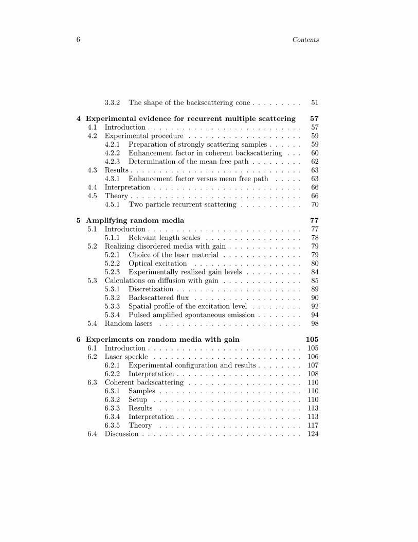
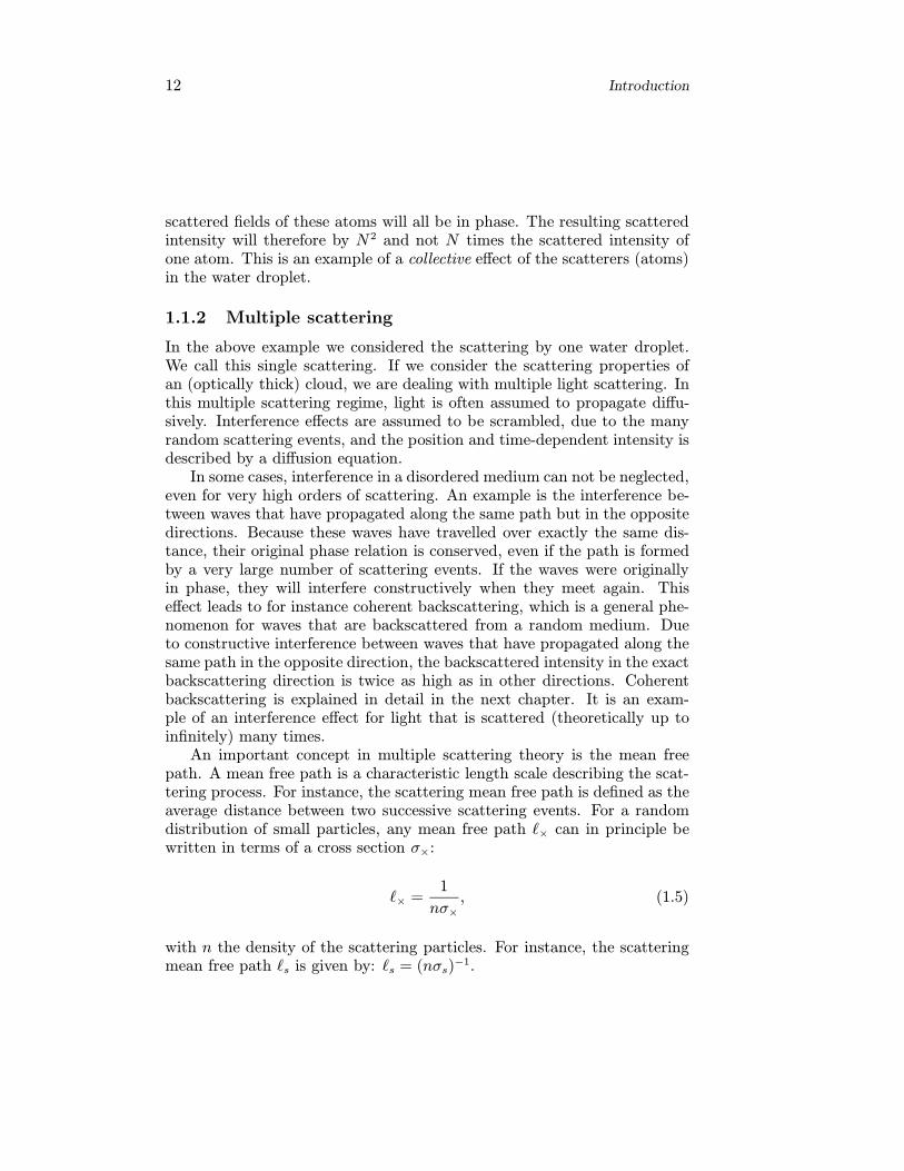
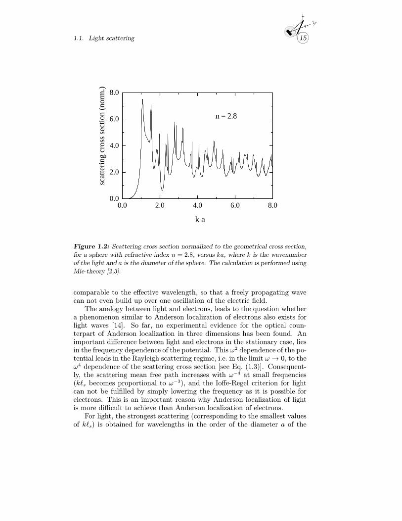
Figure 1.2: Scattering cross section normalized to the geometrical cross section,
for a sphere with refractive index n = 2.8, versus ka, where k is the wavenumber
of the light and a is the diameter of the sphere. The calculation is performed using
Mie-theory [2,3].
comparable to the effective wavelength, so that a freely propagating wavecan not even build up over one oscillation of the electric field.
The analogy between light and electrons, leads to the question whethera phenomenon similar to Anderson localization of electrons also exists forlight waves [14]. So far, no experimental evidence for the optical coun-terpart of Anderson localization in three dimensions has been found. Animportant difference between light and electrons in the stationary case, liesin the frequency dependence of the potential. This ω2 dependence of the po-tential leads in the Rayleigh scattering regime, i.e. in the limit ω → 0, to theω4 dependence of the scattering cross section [see Eq. (1.3)]. Consequent-ly, the scattering mean free path increases with ω−4 at small frequencies(k s becomes proportional to ω−3), and the Ioffe-Regel criterion for lightcan not be fulfilled by simply lowering the frequency as it is possible forelectrons. This is an important reason why Anderson localization of lightis more difficult to achieve than Anderson localization of electrons.
For light, the strongest scattering (corresponding to the smallest valuesof k s) is obtained for wavelengths in the order of the diameter a of the
16 Introduction
pumplasertransition
fast decay
pump
fast decay
fast decay
lasertransition
0
2
1
2
0
1
0'
3-level system 4-level system
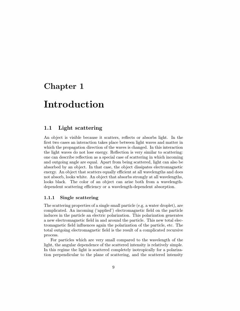
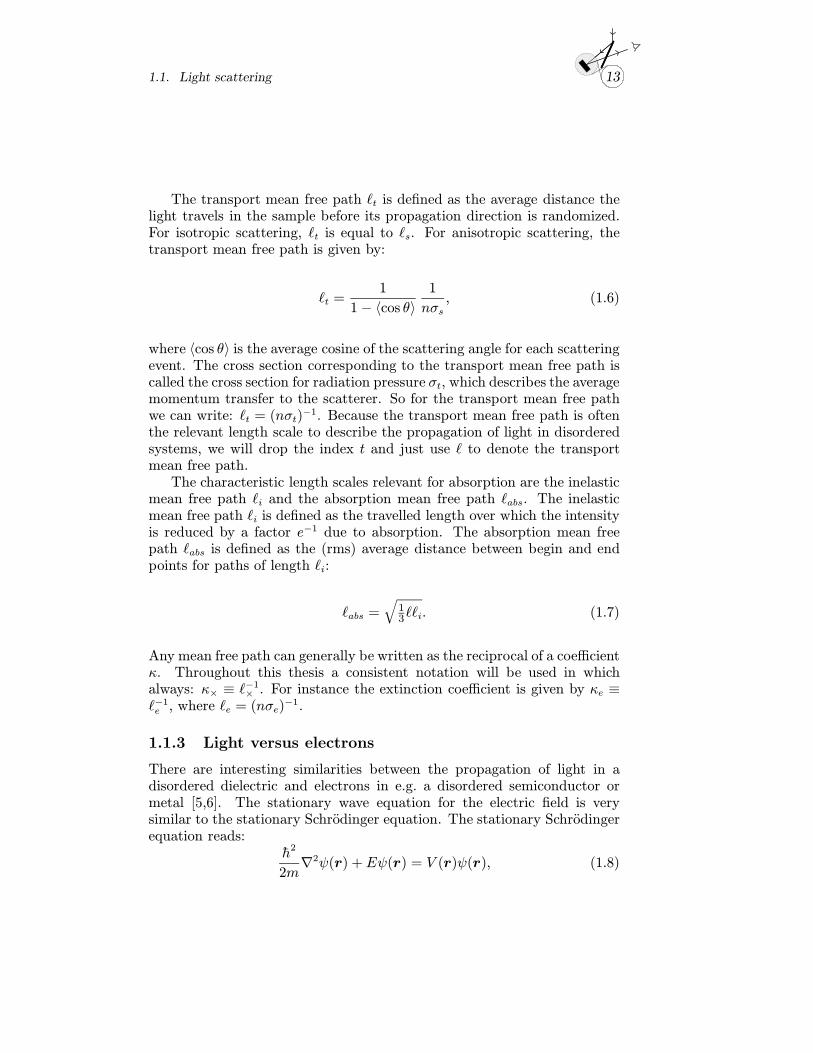
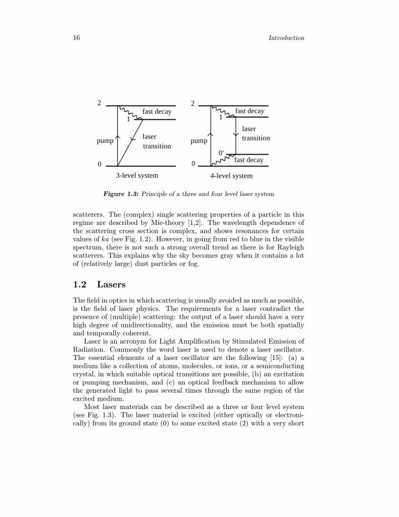
Figure 1.3: Principle of a three and four level laser system
scatterers. The (complex) single scattering properties of a particle in thisregime are described by Mie-theory [1,2]. The wavelength dependence ofthe scattering cross section is complex, and shows resonances for certainvalues of ka (see Fig. 1.2). However, in going from red to blue in the visiblespectrum, there is not such a strong overall trend as there is for Rayleighscatterers. This explains why the sky becomes gray when it contains a lotof (relatively large) dust particles or fog.
1.2 Lasers
The field in optics in which scattering is usually avoided as much as possible,is the field of laser physics. The requirements for a laser contradict thepresence of (multiple) scattering: the output of a laser should have a veryhigh degree of unidirectionality, and the emission must be both spatiallyand temporally coherent.
Laser is an acronym for Light Amplification by Stimulated Emission ofRadiation. Commonly the word laser is used to denote a laser oscillator.The essential elements of a laser oscillator are the following [15]: (a) amedium like a collection of atoms, molecules, or ions, or a semiconductingcrystal, in which suitable optical transitions are possible, (b) an excitationor pumping mechanism, and (c) an optical feedback mechanism to allowthe generated light to pass several times through the same region of theexcited medium.
Most laser materials can be described as a three or four level system(see Fig. 1.3). The laser material is excited (either optically or electroni-cally) from its ground state (0) to some excited state (2) with a very short
1.2. Lasers 17
lifetime. Then the system falls rapidly back to some metastable state (1)with a lifetime ranging from a few nanoseconds to several milliseconds. Thelifetime of this state is referred to as the excited state lifetime τe. In a threelevel system, the transition from this metastable state to the ground stateis the laser transition. In a four level system, the laser transition is a tran-sition from the metastable state to a state (0’) which decays rapidly to theground state (0).
The (optical) decay of the excited metastable state occurs either byspontaneous or by stimulated emission. In a spontaneous emission process,the radiated light is isotropic and its spectrum is determined by the broad-ening of the metastable and ground state. In a stimulated emission process,the decay is initiated by an incoming wave. In that case, the emitted lighthas the same wavelength, phase, and propagation direction as the incominglight. If the ground state is populated, the reversed process will also takeplace and the incoming light is absorbed. The dynamics of the system aredescribed by a set of rate equations. For a three level system we have:
dN0(r, t)
dt= −cN0(r, t)[σ02WG(r, t) + σ01WR(r, t)] (1.12)
+ σ10cN1(r, t)WR(r, t) +1
τeN1(r, t),
anddN1(r, t)
dt= −
dN0(r, t)
dt(1.13)
where c is the speed of light, N1 and N0 are the populations of respectivelythe metastable state and the ground state, σ02, σ01, and σ10 are the crosssections for respectively absorption at the pump wavelength [(0) → (2)],absorption at the emission wavelength [(0) → (1)] and stimulated emis-sion [(1) → (0)]. Here WG(r, t) and WR(r, t) are the energy densities ofrespectively the pump light and the emitted light. The population of thethird level can be neglected due to its very short lifetime. (All populationtransferred from (0) to (2) decays almost instantly to (1).) If the energylevels are equally degenerate, the absorption cross section for a transitionequals the emission cross section: σ10 = σ01 [16]. The amplification of lightat the emission wavelength, is then determined by:
dWR(r, t)
dz= (N1 −N0)σ01WR(r, t). (1.14)
18 Introduction
We see that to obtain amplification, the population in the metastable statemust be larger than in the ground state. This situation is called inversion.To obtain this situation in a four level system is much easier, because theground state (0’) of the laser transition is nearly unpopulated.
To obtain a laser oscillator, one requires a feedback mechanism thatallows the light to pass several times through the excited laser material.This is usually achieved with an optical cavity. In the simplest geometry,this cavity exists of two parallel mirrors, of which one is partially transmit-ting. The properties of the laser emission depend strongly on this cavity.Usually, the oscillator starts from (broad banded) spontaneous emission.Subsequently only those wavelengths that ‘fit’ in the cavity are amplified,that is, the wavelength must be equal to the cavity length divided by aninteger. The spectral width of the emission is determined by the quality ofthe cavity and the gain, and can be extremely small. Naturally, also thedirection of the laser output is determined by the cavity.
To obtain a high quality coherent laser oscillator, scattering is avoidedas much as possible. The question arises, what would happen if one com-bines optical amplification with disorder. One could for instance study theemission from an excited laser material (not placed between cavity mirrors)in which one introduces a large amount of scattering. Due to the presenceof relatively strong scattering, the residence time of light in the medium(and thereby the energy density of the light) increases, which will affect thespectral properties of the emission. Is it possible to obtain a laser oscillatoras described above, in a medium in which the light is multiply scattered?In such a system, an optical feedback mechanism would be provided byrandom scattering. Also, it can be interesting to study the effect of gain onknown multiple scattering interference phenomena like coherent backscat-tering. Due to the presence of gain, the contribution from long light pathswill become more important. Also, due to the divergens of the intensityat infinite path lengths, the scattering properties of an amplifying randommedium will depend critically on the sample geometry and size.
1.3 This thesis
In chapter 2 of this thesis, an introduction is given to multiple scatteringtheory for light. We will introduce diffusion theory for light in a disor-dered dielectric, and calculate explicitly the diffusion propagator for a slabgeometry. Also we will explain the Green’s function perturbation theory,commonly used to treat multiple light scattering. We will calculate ex-plicitly coherent backscattering from a disordered slab in the diffusion ap-
1.3. This thesis 19
proximation. Throughout this thesis we will refer to the various conceptsintroduced in chapter 2.
In chapter 3, we will go into the experimental aspects of coherentbackscattering. We will describe a new technique to record coherentbackscattering cones and show some results in the weak scattering regime.
This technique is applied in chapter 4, to find experimental evidence forrecurrent scattering of light in the strong scattering regime, close to whereAnderson localization of light could be expected. Also we will present acalculation on the enhancement factor in coherent backscattering in thestrong scattering regime, which supports the interpretation of our experi-mental results.
In chapter 5, we will go into the various aspects of the combination ofoptical amplification with multiple scattering. We will demonstrate howan amplifying random medium can be realized, and investigate the char-acteristics of the emission from such a medium from a theoretical point ofview.
In chapter 6, we will describe scattering experiments from amplifyingrandom media, of which coherent backscattering is of particular interest.Also a calculation is presented on coherent backscattering from amplifyingdisordered structures.
20
References and notes
[1] G. Mie, Ann. Physik 25, 337 (1908).[2] H.C. van de Hulst, Light Scattering by Small Particles, (Dover, New
York, 1981).[3] G.F. Bohren and D.R. Huffman, Absorption and Scattering of Light by
Small Particles (Wiley, New York, 1983).[4] R.P. Feynman, Lectures on Physics vol. 1, (Addison-Wesley, Menlo
Park, California, 1977).[5] Analogies in Optics and Micro Electronics, edited by W. van Haeringen
and D. Lenstra (Kluwer, Dordrecht, 1990).[6] P. Sheng, Introduction to Wave Scattering, Localization, and Meso-
scopic Phenomena (Academic Press, San Diego, 1995).[7] M.P. van Albada, B.A. van Tiggelen, A. Lagendijk, and A. Tip, Phys.
Rev. Lett. 66, 3132 (1991).[8] A. Lagendijk and B.A. van Tiggelen, to be published in Physics reports
(1995).[9] P.W. Anderson, Phys. Rev. 109, 1492 (1958); Anderson Localization,
edited by T. Ando and H. Fukuyama, in Springer proceedings in physics28 (Springer, Berlin, 1988).
[10] P.A. Lee and T.V. Ramakrishnan, Rev. of Modern Phys. 57, 287(1985).
[11] B.L. Altshuler, A.G. Aronov, D.E. Khmel’nitskii, and A.I. Larkin, inQuantum Theory of Solids, edited by I.M. Lifshits (MIR Publishers,Moskva, 1983).
[12] D. Vollhardt and P. Wolfle, in Electronic Phase Transitions, ModernProblems in Condensed Matter Sciences 32, edited by W. Hanke andYu. V. Kopaev (North-Holland, Amsterdam, 1992).
[13] A.F. Ioffe and A.R. Regel, Progr. Semiconductors 4, 237 (1960); N.F.Mott, Metal-Insulator Transitions (Taylor and Francis, London, 1974).
[14] Scattering and Localization of Classical Waves in Random Media inWorld Scientific Series on Directions in Condensed Matter Physics 8,edited by P. Sheng (World Scientific, Singapore, 1990).
[15] A.E. Siegman, Lasers (University Science Books, Mill Valley, Califor-nia, 1986).
[16] Usually the three or four levels picture used to describe a laser materialis a simplification of a much more complicated system consisting ofmany energy levels. In that case it not generally true that the emissionand absorption cross sections are equal.
Chapter 2
Multiple scattering theory
2.1 Introduction
The propagation of light in a any medium is generally described byMaxwell’s equations for the electric and magnetic field. To calculate theelectric field in a disordered dielectric like white paint or a colloidal suspen-sion, one is faced with solving a wave equation with a randomly varyingrefractive index. In section 2.3, it will be shown how Green’s function the-ory is often used to treat this problem. A Green’s function G(r1, r2) thatdescribes the propagation of the electric field in a random medium is intro-duced, as well as the four point vertex Γ(r1, r2; r3, r4) that describes thepropagation of the intensity. These concepts are introduced without goinginto great detail. For a thorough treatment of multiple light scatteringwe refer to the literature on this subject [1–4]. In section 2.4, it will beshown how the backscattered intensity from a disordered medium can becalculated explicitly in the diffusion approximation. Because the diffusionapproximation forms an important concept in multiple scattering theory, westart with introducing the diffusion equation for light in disordered media.
2.2 Diffusion of light
In the diffusion approximation, the propagation of the intensity is describedas a random walk with a characteristic mean free path . Only the intensityand not the electric field itself is considered, so the wave character of thelight is not taken into account. Usually also the vector nature of light isdisregarded. In reality, there are two polarization channels over which thelight is distributed in the scattering process. In chapter 3 we will show that
21
22 Multiple scattering theory
good agreement is found between scalar diffusion theory and experimentaldata for light backscattered from a disordered sample. In the diffusionapproximation, the intensity I(r, t) is determined by a diffusion equation:
∂I(r, t)
∂t= D∇2I(r, t)−
v
iI(r, t), (2.1)
where D is the diffusion constant given by D = 13 v with the transport
mean free path, v is the transport velocity for the light inside the medium,and i is the inelastic mean free path.
2.2.1 Stationary solution for a slab
Most of the samples that are studied experimentally have a slab geometry.In the this subsection, the stationary solution to the diffusion equation iscalculated for such a slab geometry. Starting point is Eq. (2.1). In thestationary case, the time derivative on the left hand side is zero. We canaccount for an incoming intensity by adding a source function S(r) on theright hand side. This yields:
0 = 13 2∇2I(r)− κiI(r) + S(r), (2.2)
Defining the intensity propagator F (r1, r2) as the solution of:
13 2∇2F (r1, r2)− κi F (r1, r2) = −δ(r1 − r2), (2.3)
one can write the intensity as:
I(r1) =
∫dr2 F (r1, r2)S(r2), (2.4)
where the integral is taken over the volume of the scattering medium. Theintensity propagator F (r1, r2) describes the propagation of the intensity ina disordered slab in the diffusion approximation. By introducing F (r1, r2),the problem of solving the stationary diffusion equation has been reducedto finding the solution of Eq. (2.3), which is independent of S(r).
2.2. Diffusion of light 23
It is convenient to choose the orientation of the slab such that its in-terface is perpendicular to the z-axis. Then the system is translationallyinvariant over x and y, and one can use the Fourier transform:
F (q⊥, z1, z2) =
∫dr⊥F (r1, r2)e
ir⊥·q⊥ , (2.5)
where r⊥ = r1⊥ − r2⊥ is perpendicular to z. After Fourier transformingEq. (2.3), one obtains:
13 2
(∂2
∂z21− q2⊥
)F (q⊥, z1, z2)− κiF (q⊥, z1, z2) = −δ(z1 − z2). (2.6)
From radiative transfer theory [5], it is known that the diffuse intensityat the front and rear interface (z = 0 and z = L) of the sample is notzero, but that the appropriate boundary condition for a slab is found bytaking the intensity zero at a distance z0 from the interface. The valueof z0 depends on the refractive index contrast between the sample and itssurrounding medium [6]. For an index matched sample interface its valueis: z0 ≈ 0.7104 [5]. Solving Eq. (2.6) with this boundary condition onefinds:
F (q⊥, z1, z2) = F (q⊥, zs, zd) =3 cosh[α(L−zs)]− 3 cosh[α(L+2z0−|zd|)]
2 2 α sinh[α(L+ 2z0)],
(2.7)
where zs ≡ z1+z2, zd ≡ z1−z2, L is the slab thickness, and α ≡√ −2abs + q2⊥
with abs the absorption length in the medium. One can identify q⊥ withk1⊥+k2⊥, where k2⊥ and k1⊥ are the perpendicular components of respec-tively the incoming and outgoing wavevector. With the intensity propa-gator F (q⊥, z1, z2), one can calculate the diffuse intensity in a disorderedslab from any source S(r). For an incoming plane wave from z = −∞,the source function is S(z) = S0 exp (−zκe), where κe is the extinction rategiven by κe ≡ −1e = −1s + −1i . In section 2.4, we will show how one canuse the intensity propagator F (r1, r2) to calculate coherent backscatteringin the diffusion approximation.
24 Multiple scattering theory
2.3 Multiple scattering of waves
In this section, the formalism is introduced which is commonly used todescribe multiple scattering of light waves. Starting point is the set ofMaxwell’s equations for the electric and magnetic field. Green’s functiontheory is used to derive perturbation expansions both for the electric fieldand the intensity. Also the (Feynman) diagrams are introduced that canbe used to simplify the notation for the electric field and the intensity.
2.3.1 Electric field
Starting from Maxwell’s equations, the electric field can be shown to fulfillthe time-dependent wave equation [7]:
∇2E(r, t) +∇E(r, t) ·∇ε(r)
ε(r)−
ε(r)
c20
∂2E(r, t)
∂t2= 0. (2.8)
The second term in this equation, containing the gradient of ε(r), is zeroin regions of space where ε(r) is constant. We will regard a collection ofparticles with a constant refractive index in a surrounding medium withanother constant refractive index, so ε(r) is constant inside and outsidethe particles. In that case, the second term in Eq. (2.8) determines theboundary condition for the electric field at the particle boundary, and iszero elsewhere. By using a Fourier transformation with respect to time,the explicit time dependence in Eq. (2.8) can be removed, and all harmon-ics of the resulting Fourier representation will follow the time-independentHelmholtz equation:
∇2E(r) + (ω/c0)2ε(r)E(r) = 0, (2.9)
where E(r) denotes one of the field components of the electric field, insideor outside the scatterers. The same equation holds for the magnetic fieldcomponents. Here ε(r) is the (random) place-dependent dielectric constantof the system, ω the frequency of the electric field, and c0 the vacuum speedof light. The wave equation can be written as:
∇2E(r) + (ω/c0)2E(r) = V (r)E(r), (2.10)
where V (r) is the scattering potential defined as V (r) ≡ −(ω/c0)2
[ε(r)− 1]. For a collection of point like scatterers with polarizability α0, in
2.3. Multiple scattering of waves 25
a surrounding medium with dielectric constant 1, the scattering potentialis given by:
V (r) = −α0(ω/c0)2∑i
δ(r − ri), (2.11)
with ri the positions of the scatterers. For a point like scatterer withdielectric constant ε1 and radius a in vacuum, the polarizability is givenby α0 = a3(ε1 − 1)/(ε1 + 2). Introducing the Green’s function G0(r1, r2)as the solution of:
∇2G0(r1, r2) + (ω/c0)2G0(r1, r2) = −δ(r1 − r2), (2.12)
one can write the solution to Eq. (2.10) formally as:
E(r1) = Ein(r1)−∫dr2G0(r1, r2)V (r2)E(r2), (2.13)
where Ein(r1) is a solution of the homogeneous wave equation obtained bytaking V (r) = 0 in Eq. (2.10). Ein(r1) represents the incoming coherentwave. G0(r1, r2) is also referred to as the bare Green’s function and de-scribes the propagation of the field in a medium without scatterers. It isgiven by:
G0(r1, r2) =e−ik |r1−r2 |
4π |r1−r2 |, (2.14)
with k = ω/c0. By iterating the recursion relation Eq. (2.13), one obtainsthe following perturbation series for the electric field:
E(r1)=Ein(r1)−∫dr2 G0(r1, r2)V (r2)Ein(r2) (2.15)
+
∫∫dr2dr3 G0(r1, r2)V (r2)G0(r2, r3)V (r3)Ein(r3)
−∫∫∫
dr2 .. dr4G0(r1, r2)V (r2)G0(r2, r3)V (r3)G0(r3, r4)V (r4)Ein(r4)+· · · ,
where all integrals are taken over the volume of the sample. The aboveexpression depends on Ein. To describe the propagation of the field in the
26 Multiple scattering theory
medium independently of Ein, we use the total Green’s function G(r1, r2)which is defined as the solution of:
∇2G(r1, r2) + (ω/c0)2ε(r)G(r1, r2) = −δ(r1 − r2). (2.16)
The Green’s function G(r1, r2) describes the field at any point r1 in themedium, due to a source at r2. The perturbation series for G(r1, r2) is:
G(r1, r2) = G0(r1, r2)−∫draG0(r1, ra)V (ra)G0(ra, r2) (2.17)
+
∫∫dradr bG0(r1, ra)V (ra)G0(ra, r b)V (r b)G0(r b, r2)− · · · · · · .
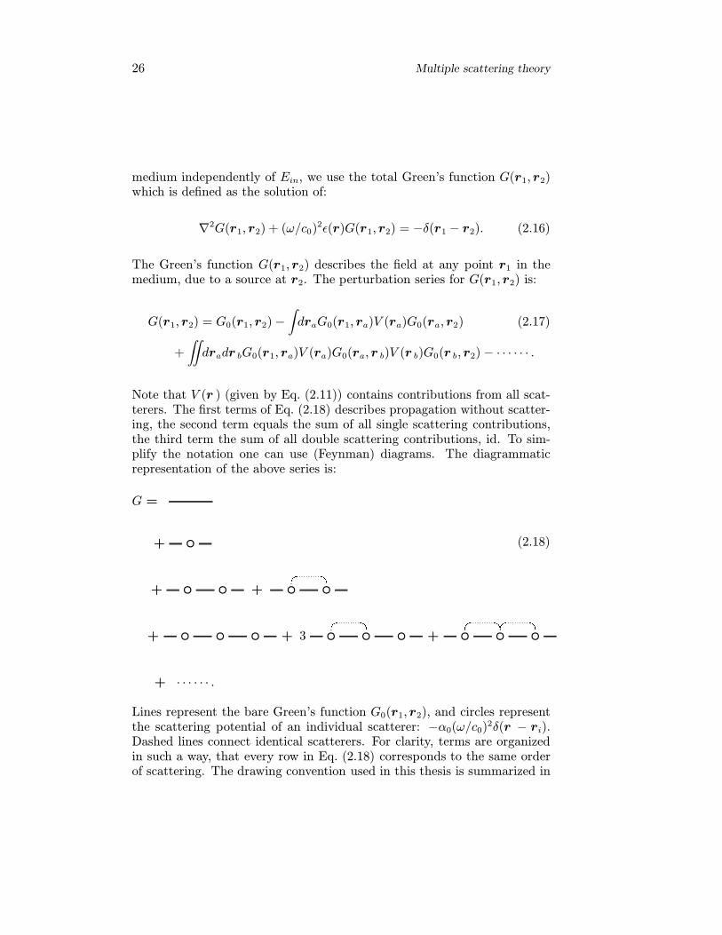
Note that V (r ) (given by Eq. (2.11)) contains contributions from all scat-terers. The first terms of Eq. (2.18) describes propagation without scatter-ing, the second term equals the sum of all single scattering contributions,the third term the sum of all double scattering contributions, id. To sim-plify the notation one can use (Feynman) diagrams. The diagrammaticrepresentation of the above series is:
G =
(2.18)+ ◦
+ ◦ ◦ + ◦'& %$◦
+ ◦ ◦ ◦ + 3 ◦'& %$◦ ◦ + ◦
'& %$◦'& %$◦
+ · · · · · · .
Lines represent the bare Green’s function G0(r1, r2), and circles representthe scattering potential of an individual scatterer: −α0(ω/c0)2δ(r − ri).Dashed lines connect identical scatterers. For clarity, terms are organizedin such a way, that every row in Eq. (2.18) corresponds to the same orderof scattering. The drawing convention used in this thesis is summarized in
2.3. Multiple scattering of waves 27
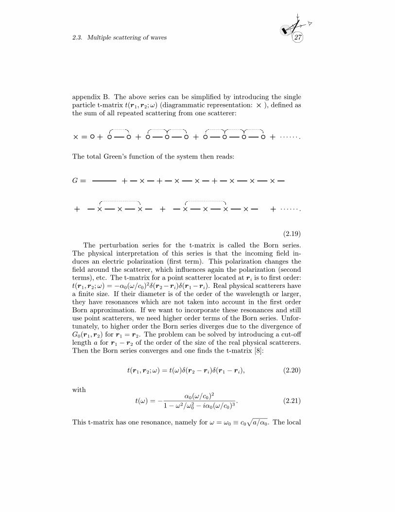
appendix B. The above series can be simplified by introducing the singleparticle t-matrix t(r1, r2;ω) (diagrammatic representation: × ), defined asthe sum of all repeated scattering from one scatterer:
× = ◦+ ◦'& %$◦ + ◦
'& %$◦'& %$◦ + ◦
'& %$◦'& %$◦'& %$◦ + · · · · · · .
The total Green’s function of the system then reads:
G = + × + × × + × × ×
+ ×'& %$
× × + ×'& %$
× × × + · · · · · · .
(2.19)
The perturbation series for the t-matrix is called the Born series.The physical interpretation of this series is that the incoming field in-duces an electric polarization (first term). This polarization changes thefield around the scatterer, which influences again the polarization (secondterms), etc. The t-matrix for a point scatterer located at ri is to first order:t(r1, r2;ω) = −α0(ω/c0)2δ(r2−ri)δ(r1−ri). Real physical scatterers havea finite size. If their diameter is of the order of the wavelength or larger,they have resonances which are not taken into account in the first orderBorn approximation. If we want to incorporate these resonances and stilluse point scatterers, we need higher order terms of the Born series. Unfor-tunately, to higher order the Born series diverges due to the divergence ofG0(r1, r2) for r1 = r2. The problem can be solved by introducing a cut-offlength a for r1 − r2 of the order of the size of the real physical scatterers.Then the Born series converges and one finds the t-matrix [8]:
t(r1, r2;ω) = t(ω)δ(r2 − ri)δ(r1 − ri), (2.20)
with
t(ω) = −α0(ω/c0)
2
1− ω2/ω20 − iα0(ω/c0)3. (2.21)
This t-matrix has one resonance, namely for ω = ω0 ≡ c0√a/α0. The local
28 Multiple scattering theory
electric polarization P (ω, r) induced by the total electric field is given by:
P (ω, r) = [ε(r)− 1]E(ω, r). (2.22)
Using the definition of the t-matrix, one can write this polarization (for asystem of one scatterer) in terms of the incoming field Ein(ω, r) as:
P (ω, r) = −c20ω2
V (ω, r)E(ω, r) = −c20ω2
t(ω)Ein(ω, r). (2.23)
This means that the t-matrix can be written as a polarizability α(ω) of thescatterer, induced by the incoming field Ein(ω, r):
α(ω) = −c20ω2
t(ω) . (2.24)
The scattering cross section and extinction cross section in terms of thet-matrix are given by: σs = (4π)−1|t(ω)|2 and σe = −(c0/ω) Im[t(ω)]. Fornon absorbing particles the extinction cross section is equal to the scatteringcross section, which yields the following condition for the t-matrix:
1
4π|t(ω)|2= −
c0ωIm[t(ω)]. (2.25)
The above relation is known as the optical theorem.The terms in the perturbation series of Eq. (2.19) with dashed lines con-
necting identical scatterers, are called recurrent scattering events. Theseare events in which a wave is scattered by a specific scatterer, scatteredby at least one other scatterer and then returns to this specific scatterer.For relatively weak scattering, recurrent scattering events can be neglect-ed. This approximation is called the ‘self-avoiding multiple scattering ap-proximation’ (SAMS). In chapter 4 we will discuss the breakdown of thisapproximation at very strong scattering. There we will show how recurrentevents can influence the backscattered intensity from a strongly scatteringsample.
The total Green’s function G(r1, r2) depends on the positions of thescatterers. A useful quantity is the averaged or ‘dressed’ Green’s functionG(r1−r2), which is obtained by averaging G(r1, r2) over the positions of the
2.3. Multiple scattering of waves 29
scatterers. In the SAMS approximation G(r1−r2) can be calculated fromEq. (2.19), by Fourier transforming to momentum space. In momentumspace the summation can be performed and after transforming back to realspace one finds:
G(r1 − r2) ≡ 〈G(r1, r2)〉 =e−iK |r1−r2|
4π |r1−r2|, (2.26)
where K =√(ω/c0)2 + nt is the (complex) effective k-vector for the light
inside the sample, with n the density of scatterers.
2.3.2 Intensity
The intensity is defined as the energy that crosses a unit area per unit oftime. It is given by the magnitude of the cycle average of the Poyntingvector E×B, which can be written as:
I(r) =c0 n
2|E(r) |2, (2.27)
with c0 the vacuum speed of light, and n the refractive index of the medium.In terms of the total Green’s function G(r1, r2), the intensity is given by:
I(r) ≡c0 n
2E(r)E∗(r) =
c0 n
2
∫∫dr1dr2G(r , r1)G
∗(r , r2)Ein(r1)E∗in(r2),
(2.28)
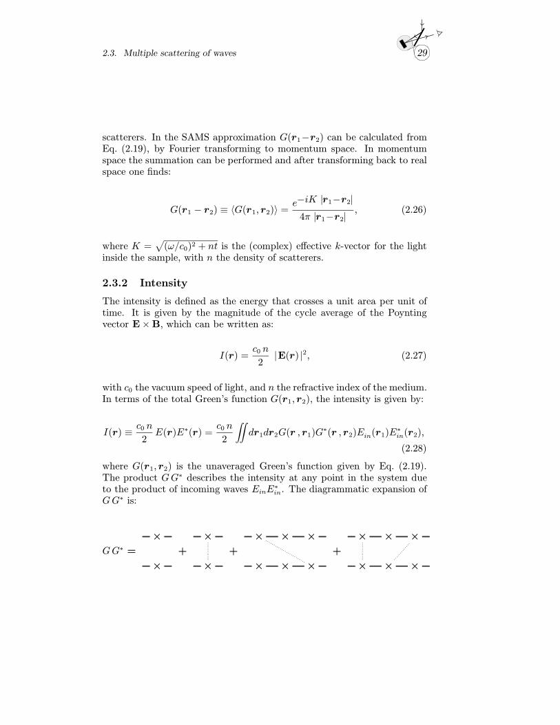
where G(r1, r2) is the unaveraged Green’s function given by Eq. (2.19).The product GG∗ describes the intensity at any point in the system dueto the product of incoming waves EinE
∗in. The diagrammatic expansion of
GG∗ is:
GG∗ =
×
×
+
×
×
+
× × ×
× × ×
+
× × ×
× × ×
30 Multiple scattering theory
+
× ×
× ×
+
× × ×
× × ×
+
×'& %$
× ×
× × ×
+ · · · · · · .
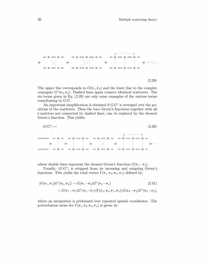
(2.29)
The upper line corresponds to G(r1, r2) and the lower line to the complexconjugate G∗(r3, r4). Dashed lines again connect identical scatterers. Thesix terms given in Eq. (2.29) are only some examples of the various termscontributing to GG∗.
An important simplification is obtained if GG∗ is averaged over the po-sitions of the scatterers. Then the bare Green’s functions together with allt-matrices not connected by dashed lines, can be replaced by the dressedGreen’s function. This yields:
〈GG∗〉 = (2.30)
+
×
×
+
× ×
× ×
+
× ×
× ×
+
×'& %$
× ×
× × ×
+ · · ·
where double lines represent the dressed Green’s function G(r1−r2).Usually, 〈GG∗〉 is stripped from its incoming and outgoing Green’s
functions. This yields the total vertex Γ(r1, r2; r3, r4) defined by:
〈G(r1, r2)G∗(r3, r4)〉 = G(r1−r2)G∗(r3−r4) (2.31)
+G(r1−r5)G∗(r3−r7)〈Γ(r5, r6; r7, r8)〉G(r6−r2)G
∗(r8−r4),
where an integration is performed over repeated spatial coordinates. Theperturbation series for Γ(r1, r2; r3, r4) is given by:
2.4. Backscattered intensity 31
〈Γ〉 =
×
×
+
× ×
× ×
+
× ×
× ×
+
×'& %$
× ×
× × ×
+
× × ×
× × ×
+ · · ·
(2.32)
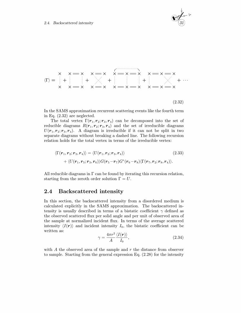
In the SAMS approximation recurrent scattering events like the fourth termin Eq. (2.32) are neglected.
The total vertex Γ(r1, r2; r3, r4) can be decomposed into the set ofreducible diagrams R(r1, r2; r3, r4) and the set of irreducible diagramsU(r1, r2; r3, r4). A diagram is irreducible if it can not be split in twoseparate diagrams without breaking a dashed line. The following recursionrelation holds for the total vertex in terms of the irreducible vertex:
〈Γ(r1, r2; r3, r4)〉 = 〈U(r1, r2; r3, r4)〉 (2.33)
+ 〈U(r1, r5; r3, r6)〉G(r5−r7)G∗(r6−r8)〈Γ(r7, r2; r8, r4)〉.
All reducible diagrams in Γ can be found by iterating this recursion relation,starting from the zeroth order solution Γ = U .
2.4 Backscattered intensity
In this section, the backscattered intensity from a disordered medium iscalculated explicitly in the SAMS approximation. The backscattered in-tensity is usually described in terms of a bistatic coefficient γ defined asthe observed scattered flux per solid angle and per unit of observed area ofthe sample at normalized incident flux. In terms of the average scatteredintensity 〈I(r)〉 and incident intensity I0, the bistatic coefficient can bewritten as:
γ =4πr2
A
〈I(r)〉
I0, (2.34)
with A the observed area of the sample and r the distance from observerto sample. Starting from the general expression Eq. (2.28) for the intensity
32 Multiple scattering theory
and after averaging over the positions of the scatterers using the definitionof the total vertex, one obtains for the scattered intensity:
〈I(r)〉=c0 n
2
∫dr1..dr4G(r−r1)G
∗(r−r3)〈Γ(r1, r2; r3, r4)〉〈Ein(r2)E∗in(r4)〉.
(2.35)
The dressed Green’s function G(r − r1) and the complex conjugateG∗(r −r3) describe the propagation of the scattered intensity towards thepoint of observation and are given by Eq. (2.26). For backscattering,G(r −r1) can be approximated by:
G(r −r1) −eikr
4πre−iks·r1 −
12κez1µ
−1s , (2.36)
with r1 inside the slab and r far outside the slab, where we have used that:
iK |r−r1|≈ iK
(r −r · r1r
)≈ ikr − iK · r1, (2.37)
with K = ks +12 iκeµ
−1s z. Here k = ω/c0, ks is the outgoing wavevector,
κe is the extinction coefficient, and µs = cos θ, with θ the angle betweenks and z. For the incoming wave Ein(r ) we take a normalized plane waveperpendicular to the sample surface, which is damped inside the sample byκe:
Ein(r ) = E0 e(ik − 12κe)z . (2.38)
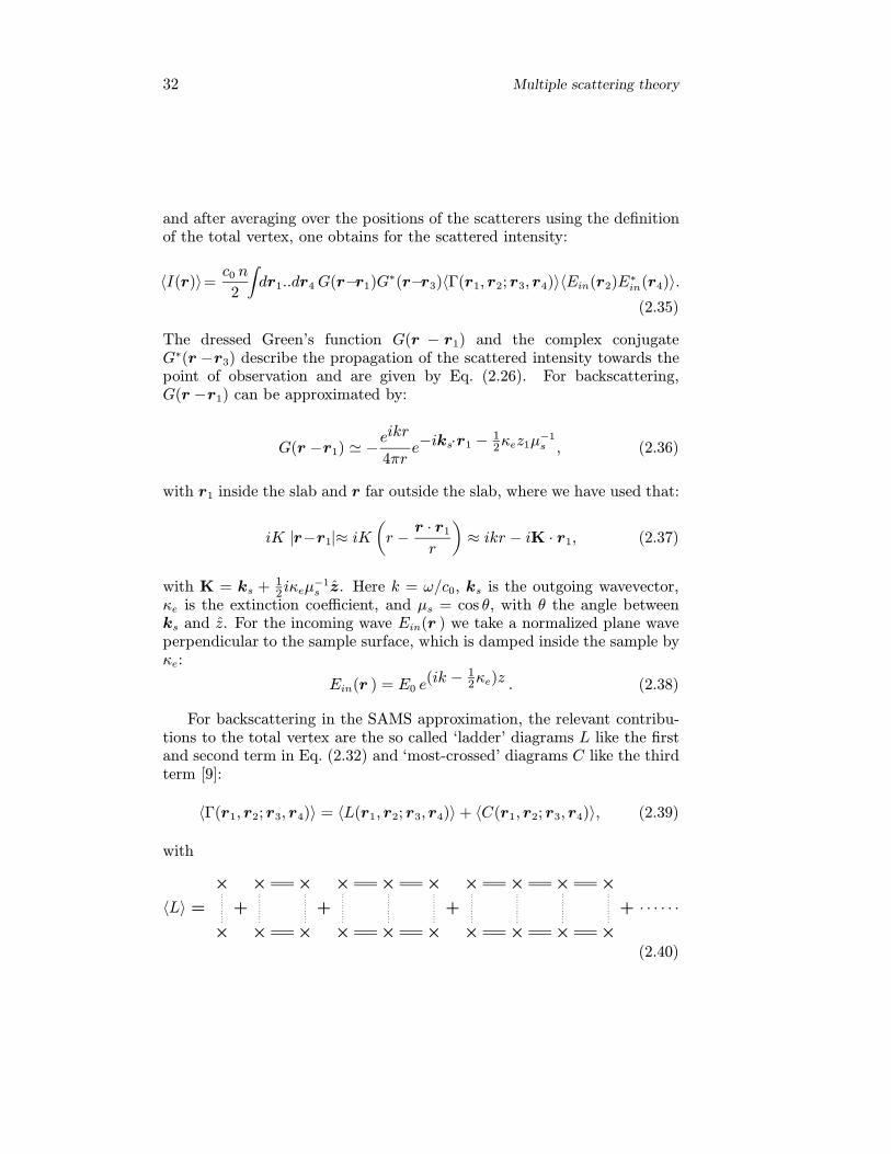
For backscattering in the SAMS approximation, the relevant contribu-tions to the total vertex are the so called ‘ladder’ diagrams L like the firstand second term in Eq. (2.32) and ‘most-crossed’ diagrams C like the thirdterm [9]:
〈Γ(r1, r2; r3, r4)〉 = 〈L(r1, r2; r3, r4)〉+ 〈C(r1, r2; r3, r4)〉, (2.39)
with
〈L〉 =
×
×
+
× ×
× ×
+
× × ×
× × ×
+
× × × ×
× × × ×
+ · · · · · ·
(2.40)
2.4. Backscattered intensity 33
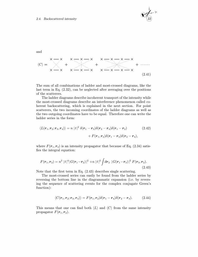
and
〈C〉 =
× ×
× ×
+
× × ×
× × ×
+
× × × ×
× × × ×
+ · · · · · ·
(2.41)
The sum of all combinations of ladder and most-crossed diagrams, like thelast term in Eq. (2.32), can be neglected after averaging over the positionsof the scatterers.
The ladder diagrams describe incoherent transport of the intensity whilethe most-crossed diagrams describe an interference phenomenon called co-herent backscattering, which is explained in the next section. For pointscatterers, the two incoming coordinates of the ladder diagrams as well asthe two outgoing coordinates have to be equal. Therefore one can write theladder series in the form:
〈L(r1, r2; r3, r4)〉 = n |t |2 δ(r1 − r3)δ(r2 − r4)δ(r1 − r2) (2.42)
+ F (r1, r2)δ(r1 − r3)δ(r2 − r4),
where F (r1, r2) is an intensity propagator that because of Eq. (2.34) satis-fies the integral equation:
F (r1, r2) = n2 |t |4|G(r1−r2) |2 +n |t |2
∫dr2 |G(r1−r3) |
2 F (r3, r2).
(2.43)Note that the first term in Eq. (2.43) describes single scattering.
The most-crossed series can easily be found from the ladder series byreversing the bottom line in the diagrammatic expansion (i.e. by revers-ing the sequence of scattering events for the complex conjugate Green’sfunction):
〈C(r1, r2; r3, r4)〉 = F (r1, r2)δ(r1 − r4)δ(r2 − r3). (2.44)
This means that one can find both 〈L〉 and 〈C〉 from the same intensitypropagator F (r1, r2).
34 Multiple scattering theory
This provides us with all the ingredients necessary to calculate thebistatic coefficient for a semi infinite slab in the xy-plane, illuminated bya plane wave from z = −∞. It is convenient to separate the total bistaticcoefficient γt into the contribution from most-crossed diagrams γc and fromladder diagrams, with the latter further separated into the single scatteringcontribution γs and multiple scattering contribution γ�:
γt = γs + γ� + γc. (2.45)
Using the above expressions for 〈L〉 and 〈C〉 in Eq. (2.35), one obtains thefollowing integrals for the bistatic coefficients in backscattering:
γ�(ks) =1
4πA
∫dr1...dr4e
iks·(r1 − r3)e−12κeµ
−1s (z1 + z3) (2.46)
×F (r1, r2)δ(r1 − r3)δ(r2 − r4)eik(z2 − z4)e−
12κe(z2 + z4),
γc(ks) =1
4πA
∫dr1...dr4e
iks·(r1 − r3)e−12κeµ
−1s (z1 + z3) (2.47)
×F (r1, r2)δ(r1 − r4)δ(r2 − r3)eik(z2 − z4)e−
12κe(z2 + z4),
and
γs(ks) =1
4πA
∫dr1...dr4e
iks·(r1 − r3)e−12κeµ
−1s (z1 + z3) (2.48)
× n |t |2 δ(r1 − r3)δ(r2 − r4)δ(r1 − r2)eik(z2 − z4)e−
12κe(z2 + z4),
with ks the outgoing wavevector.We have performed thesis integrals explicitly in the diffusion approxi-
mation using the diffusion propagator F (r1, r2) as calculated in section 2.2for a slab geometry. The resulting bistatic coefficients are,for single scattering:
γs(θs) =µs
1 + µs
[1− e−Lκe(1 + µ−1s )
], (2.49)
2.4. Backscattered intensity 35
for the multiple scattering ladder diagrams (describing the diffuse back-ground):
γ�(θs) =3
2 3α sin[α(L+2z0)]
Z1(1+ e−2 uL)+Z2(1− e−2 uL)+Z3e−L(v+u)
u[(u2 − α2)2 + v2(v2 − 2α2 − 2u2)](2.50)
with
Z1 = u (u2 − v2 − α2) cos[α(L+ 2z0)] + u (v2 − u2 − α2) cos(αL) (2.51)
+2uvα sin[α(L+ 2z0)] + uvαv2 − α2 − 3u2
u2 − α2sin(αL),
Z2 = v (v2 − u2 − α2) cos[α(L + 2z0)] + 2u2α sin(αL) (2.52)
−α (u2 + v2 − α2) sin[α(L+ 2z0)] + u2vu2 − v2 + 3α2
u2 − α2cos(αL),
Z3 = 2u (u2 − v2 + α2) + 2u (v2 − u2 + α2) cos(2z0 α)− 4uvα sin(2z0 α),(2.53)
and for the most-crossed diagrams (describing interference):
γc(θs) =3e−uL
2 3α sinh[α(L+ 2z0)]
1
(α2 + η2 + u2)2 − (2αη)2× (2.54)
[−2(α2 + η2 + u2) cosh(2αz0) cos(Lη)− 4αη sinh(2αz0) sin(Lη)
+2α
u(−α2 + η2 − u2) sinh(α(L+ 2z0)) sinh(uL)
−2(α2 − η2 − u2) cos(Lη) + 2(α2 + η2 + u2) cosh(α(L+ 2z0)) cosh(uL)
+4αu sinh(αL) sinh(uL)− 2(−α2 + η2 + u2) cosh(αL) cosh(uL)].
In these expressions, the angular dependence is determined by the follow-ing parameters: η ≡ k(1 − µs), u ≡
12κe(1 + µ−1s ), v ≡ 1
2κe(1 − µ−1s ),
and α ≡√ −2abs + q2⊥ with q⊥ = k sin θ. As mentioned before, µs = cos θ,
36 Multiple scattering theory
with θ the angle between the outgoing wavevector ks and z, L is the sam-ple thickness, z0 = 0.7104 , and κe is the extinction coefficient given byκe = −1s + −1i . In the limit L → ∞ (i.e. for a semi-infinite slab), theexpression for γc reduces to:
γc(θs) =3
2 3αu
α+ u(1 − e−2αz0)
(u+ α)2 + η2(2.55)
The above solutions for the bistatic coefficients in backscattering inthe diffusion approximation were checked against the expressions given inRef. [10]. Our solutions are written in a different form to be able to comparethem with the bistatic coefficients for backscattering from an amplifyingmedium (see chapter 6).
2.5 Coherent backscattering
The physical interpretation of γ� and γc is the following. γ� describes the(incoherent) backscattered intensity due to diffusion without interference.Its angular dependence is weak (see dashed line Fig. 2.1): it decreasesslowly at larger angles. This angular dependence is due to the fact thatunder larger outgoing angles, the light travels through a larger part of thesample, having a larger chance to be scattered or absorbed. The inten-sity described by γc originates from interference between reciprocal [11]waves. This interference effect is called coherent backscattering or weaklocalization [12,13] and is a general phenomenon for waves scattered byrandom media. Because a random dielectric system obeys reciprocity, anypartial wave that propagates over some distance through the sample andthen leaves the illuminated area in the backscattering direction will havea counterpropagating counterpart that follows the same path in the oppo-site direction. These counterpropagating partial waves have travelled overthe same distance in the sample and interfere therefore constructively inthe backscattering direction. This is what is described by the most-crosseddiagrams. The angular dependence of γc is strong: it decays rapidly mov-ing away from the exact backscattering direction (see solid line Fig. 2.1).Away from exact backscattering, a phase difference develops between thecounterpropagating waves that depends on the relative orientation of thepoints where the waves leave the sample. For the ensemble of light paths,the relative phases will therefore gradually randomize. After averaging overall light paths, this leads to the cone of enhanced backscattering describedby γc.
2.5. Coherent backscattering 37
-1.5 -1.0 -0.5 0.0 0.5 1.0 1.50
1
2
3
4
5
6
7
8
γ l + γ c
Angle (rad)
0
1
2S
caled intensity
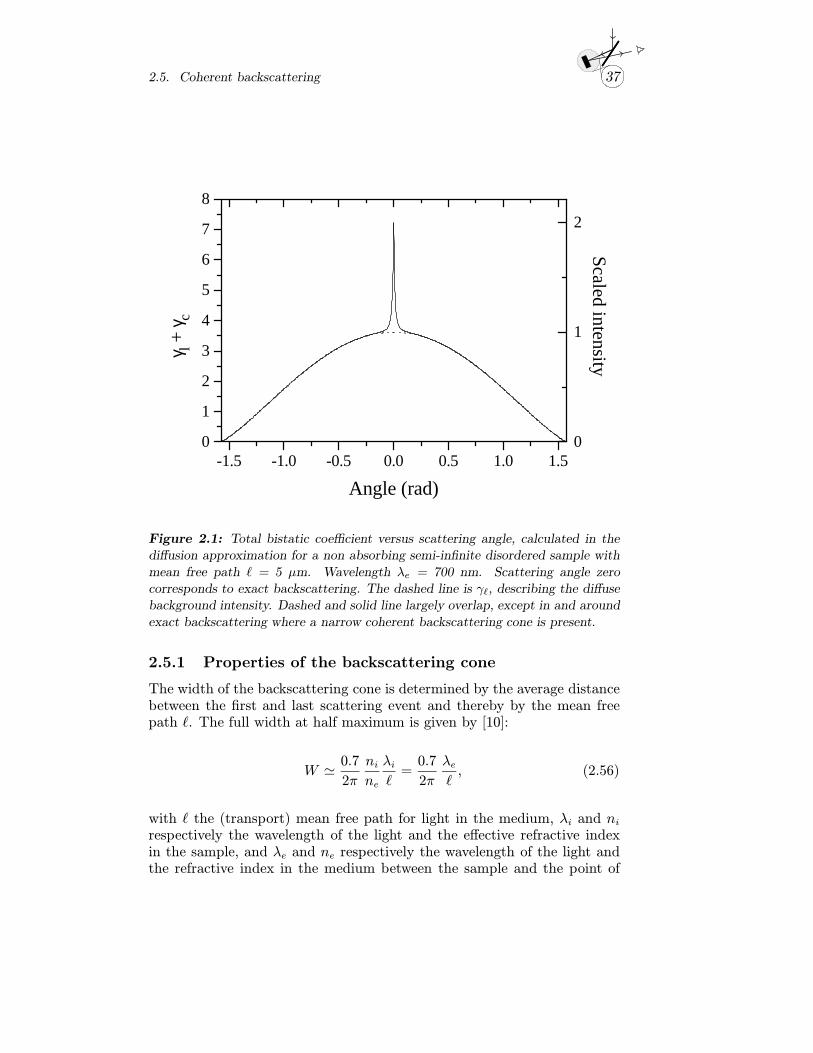
Figure 2.1: Total bistatic coefficient versus scattering angle, calculated in the
diffusion approximation for a non absorbing semi-infinite disordered sample with
mean free path = 5 µm. Wavelength λe = 700 nm. Scattering angle zero
corresponds to exact backscattering. The dashed line is γ�, describing the diffuse
background intensity. Dashed and solid line largely overlap, except in and around
exact backscattering where a narrow coherent backscattering cone is present.
2.5.1 Properties of the backscattering cone
The width of the backscattering cone is determined by the average distancebetween the first and last scattering event and thereby by the mean freepath . The full width at half maximum is given by [10]:
W 0.7
2π
nine
λi =
0.7
2π
λe , (2.56)
with the (transport) mean free path for light in the medium, λi and nirespectively the wavelength of the light and the effective refractive indexin the sample, and λe and ne respectively the wavelength of the light andthe refractive index in the medium between the sample and the point of
38 Multiple scattering theory
observation (usually air). The ratio ni/ne appears in the above equationbecause the outgoing waves are refracted by the refractive index contrastat the front sample interface. This refractive index contrast also leads tointernal reflection in the sample. Internal reflection enlarges the averagedistance between first and last scattering event because the outgoing wavesare partially backreflected in the sample. This leads to a narrowing of thebackscattering cone [6]. Internal reflection is not accounted for in Eq. (2.56).
The enhancement factor E of the backscattering cone is defined as theratio of the total intensity at exact backscattering to the diffuse backgroundintensity at exact backscattering. The diffuse background intensity is theintensity which would be expected from an incoherent addition of the scat-tered waves. In the SAMS approximation, E is given by:
E =γc + γ� + γsγ� + γs
∣∣∣∣θ=0
. (2.57)
In the exact backscattering direction γc = γ�, so if γs = 0, the enhance-ment factor is two. The single scattering contribution γs is zero for sphericalsymmetric scatterers in the helicity conserving polarization channel of thelight. For other polarizations, a single scattering contribution γs is present.Because a singly scattered wave does not have a distinct reciprocal counter-part, single scattering does not contribute to the interference. The angulardependence of γs depends on the nature of the scatterers, but is generallyweak. For point scatterers and scalar waves, it is given by Eq. (2.49). Fora treatment of single scattering from atomic and molecular systems in thex-ray regime, we refer to Ref. [14].
The shape of the backscattering cone reflects the path length distribu-tion of the light inside the sample and therefore reveals information aboutthe internal structure of the sample. If the sample consists of a randomcollection of small particles, the mean free path is inversely proportionalto the density n and scattering cross section σ of the particles. In thatcase, the width of the cone is a measure for the particle density. For morecomplex, e.g. sponge like, random structures it is difficult to identify theindividual scattering elements, in which case the width of the cone is justa measure for the scattering strength of the material. The shape of thebackscattering cone is sensitive to the sample structure at large depth be-cause the top of the cone is determined by very long light paths that havepenetrated deep into the sample (features that are due to > 104 scatteringevents can be resolved experimentally). In the theoretical case of zero ab-sorption, the top of the backscattering cone is a cusp for a semi-infinite slab:
2.5. Coherent backscattering 39
the derivative of Eq. (2.55) to θ is discontinuous at θ = 0. The existenceof a cusp is possible, due to the fact that at zero absorption, an infinitenumber of light paths contribute to the top of the cone. If absorption ispresent either at large depth or throughout the sample, the contributionfrom the longer light paths is reduced and consequently the top becomesrounded.
40
References and notes
[1] S. Chandrasekhar, Radiative transfer (Dover, New York, 1960).[2] A. Ishimaru, Wave propagation and scattering in random media, Vol. I
and II, (Academic press, New York, 1978).[3] H.C. van de Hulst, Multiple Light Scattering, Vol. I and II, (Dover,
New York, 1980).[4] U. Frish, Wave propagation in random media, in Probabilistic meth-
ods in applied mathematics, edited by A.T. Barucha-Reid, Vol. I, 76(Academic press, New York, 1968).
[5] H.C. van de Hulst and R. Stark, Astron. Astrophys. 235, 511 (1990).[6] A. Lagendijk, B. Vreeker, and P. de Vries, Phys. Lett. A 136, 81 (1989);
J.X. Zhu, D.J. Pine, and D.A. Weitz, Phys. Rev. A 44, 3948 (1991);[7] See e.g. J.D. Jackson, Classical Electrodynamics, (Wiley, New York,
1975).[8] Th.M. Nieuwenhuizen, A. Lagendijk, and B.A. van Tiggelen, Phys.
Lett. A 169, 191 (1993).[9] D. Vollhardt and P. Wolfle, Phys. Rev. B 22, 4666 (1980).[10] M.B. van der Mark, M.P. van Albada, and A. Lagendijk, Phys. Rev.
B 37, 3575 (1988) and E. Akkermans, P.E. Wolf, R. Maynard, and G.Maret, J. Phys. France 49 77 (1988).
[11] Optical measurements on linear physical systems obey the general prin-cipal of reciprocity, i.e. their results are invariant with respect to aninterchange of source and detector (see e.g. [3]). In the case of a con-servative system, reciprocity is equivalent to time–reversal symmetry.
[12] M.P. van Albada and A. Lagendijk, Phys. Rev. Lett. 55, 2692 (1985).[13] P.E. Wolf and G. Maret, Phys. Rev. Lett. 55, 2696 (1985).[14] M.J.P. Brugmans, Relaxation kinetics in disordered dense phases,
(PhD thesis, University of Amsterdam, 1995).
Chapter 3
An accurate techniqueto recordcoherent backscattering
In this chapter, a new technique is described to record the angular distribu-tion of backscattered light. The technique is accurate over a large scanningrange (500 mrad) which includes the exact backscattering direction, andthe angular resolution is high (100 µrad). The technique is particularlysuitable for the study of coherent backscattering from (very strongly scat-tering) random media. It allowed us to measure the theoretical value oftwo of the enhancement factor in coherent backscattering from a weaklyscattering sample.
3.1 Introduction
The technique to record backscattered light which is described in this chap-ter, was developed for the study of coherent backscattering from randommedia. The experimental study of coherent backscattering puts high de-mands on the accuracy of a setup. A technique suitable for coherentbackscattering experiments can therefore be applied to any situation wherethe angular distribution of backscattered light must be known accurately,for instance for backscattering experiments from rough surfaces or for thecharacterization of retro-reflectors.
41
42 An accurate technique to record coherent backscattering
laser
sample
beamdump
beamsplitter
laser
sample
mirror
+ +
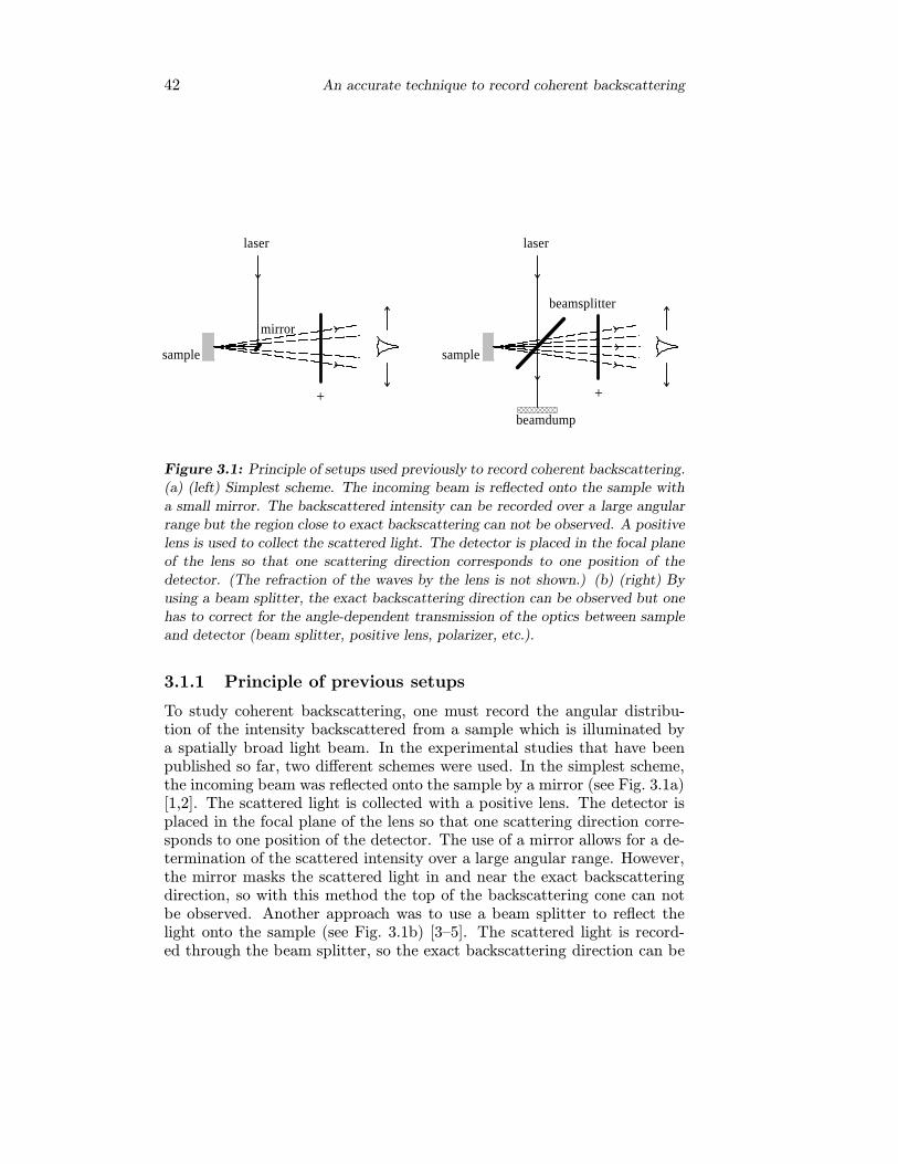
Figure 3.1: Principle of setups used previously to record coherent backscattering.
(a) (left) Simplest scheme. The incoming beam is reflected onto the sample with
a small mirror. The backscattered intensity can be recorded over a large angular
range but the region close to exact backscattering can not be observed. A positive
lens is used to collect the scattered light. The detector is placed in the focal plane
of the lens so that one scattering direction corresponds to one position of the
detector. (The refraction of the waves by the lens is not shown.) (b) (right) By
using a beam splitter, the exact backscattering direction can be observed but one
has to correct for the angle-dependent transmission of the optics between sample
and detector (beam splitter, positive lens, polarizer, etc.).
3.1.1 Principle of previous setups
To study coherent backscattering, one must record the angular distribu-tion of the intensity backscattered from a sample which is illuminated bya spatially broad light beam. In the experimental studies that have beenpublished so far, two different schemes were used. In the simplest scheme,the incoming beam was reflected onto the sample by a mirror (see Fig. 3.1a)[1,2]. The scattered light is collected with a positive lens. The detector isplaced in the focal plane of the lens so that one scattering direction corre-sponds to one position of the detector. The use of a mirror allows for a de-termination of the scattered intensity over a large angular range. However,the mirror masks the scattered light in and near the exact backscatteringdirection, so with this method the top of the backscattering cone can notbe observed. Another approach was to use a beam splitter to reflect thelight onto the sample (see Fig. 3.1b) [3–5]. The scattered light is record-ed through the beam splitter, so the exact backscattering direction can be
3.2. Experimental configuration 43
monitored. Again a positive lens is used to collect the scattered light. Thedisadvantage of this scheme is however, that one has to correct for the an-gular dependence in the transmission characteristics of the beam splitter,the positive lens, and other detection optics (e.g. a polarizer).
In both schemes it is difficult to shield stray light in a satisfactory man-ner. The fundamental problem arises from parallax: the screen that is usedto shield stray light must be placed at some distance in front of the sample.As the detector moves, the light path from sample to detector changes.Therefore, the field of view of the detector has to be larger than the solidangle under which it sees the illuminated area on the sample. In practicethis means that an amount of stray light adds to the detected signal. Thisyields an extra background in the signal which is even likely to show someangular dependence. As a result the shape and enhancement factor of thebackscattering cone can not be recorded accurately.
3.2 Experimental configuration
3.2.1 Principle of the setup
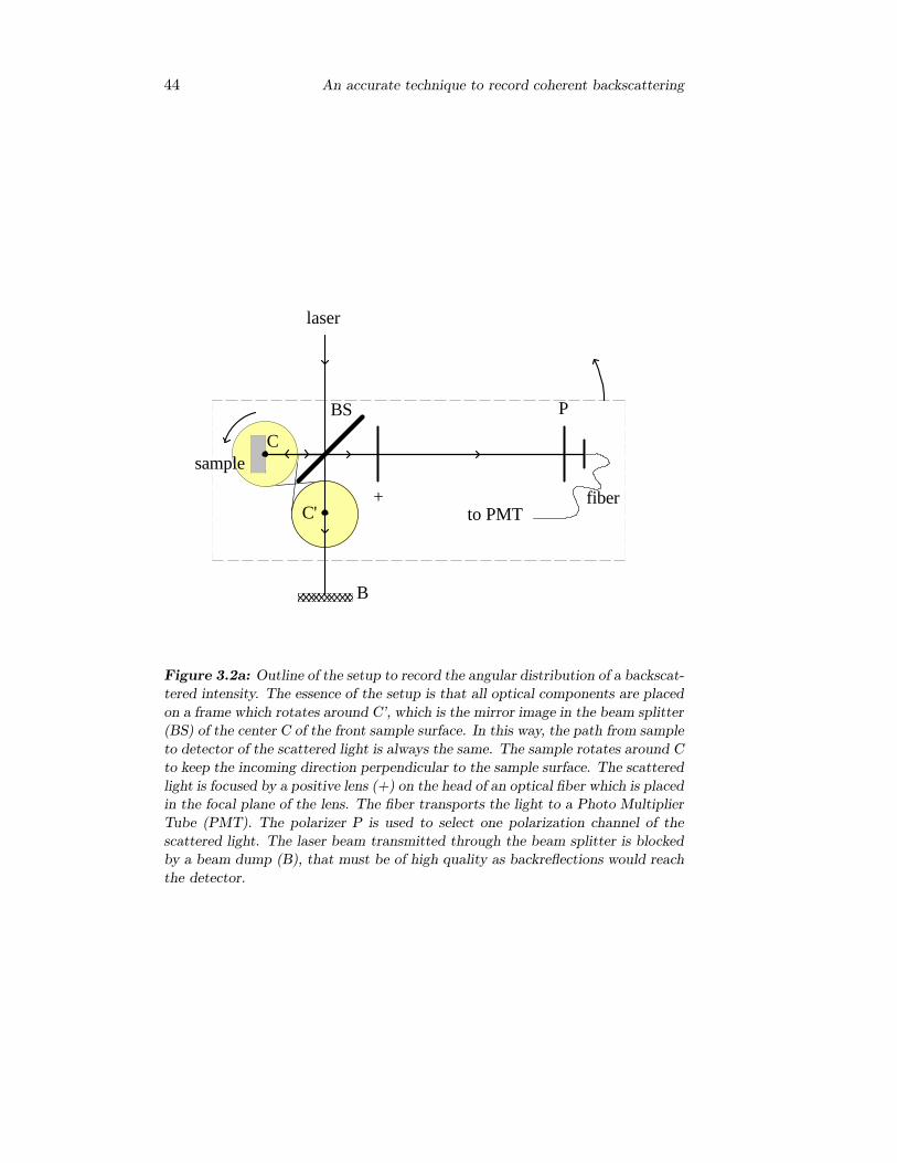
We have developed a new method which we call ‘Off-Centered Rotation’(OCR), to solve the experimental problems described above. The outlineof the setup is drawn in Fig. 3.2a. The incoming light beam is reflectedvia a beam splitter onto the sample. The scattered light is collected with apositive lens (f = 1m). The head of an optical fiber is placed in the focusof the positive lens. The fiber transports the light to a photo multipliertube. Detection optics, beam splitter and sample are placed on a rotatingframe. The center of rotation C’, is the center C of the sample surfacemirrored with respect to the plane of the beam splitter. Fig. 3.2b shows thesetup after rotation. The incoming beam is directed at C, so after rotationit still arrives at the center of the sample surface C’. With respect to theframe, the incoming direction has changed and the direction of detectionis still the same. By rotating the sample around C, the sample surface iskept at a constant angle with respect to the incoming beam. The rotation isobtained by placing the sample on a (rotatable) plateau, which is connectedby a twisted band to a disc of the same size that is fixed to the laboratoryframe. Thus the incoming direction on the sample is fixed and the angulardistribution of the scattered light is recorded. The rotation of the setup isdemonstrated around the odd page numbers of this thesis.
The scattered light always follows the same path through the beamsplitter and the detection optics. This is the major advantage of our set-
44 An accurate technique to record coherent backscattering
+to PMT
PBS
B
C
C'fiber
laser
sample
Figure 3.2a: Outline of the setup to record the angular distribution of a backscat-
tered intensity. The essence of the setup is that all optical components are placed
on a frame which rotates around C’, which is the mirror image in the beam splitter
(BS) of the center C of the front sample surface. In this way, the path from sample
to detector of the scattered light is always the same. The sample rotates around C
to keep the incoming direction perpendicular to the sample surface. The scattered
light is focused by a positive lens (+) on the head of an optical fiber which is placed
in the focal plane of the lens. The fiber transports the light to a Photo Multiplier
Tube (PMT). The polarizer P is used to select one polarization channel of the
scattered light. The laser beam transmitted through the beam splitter is blocked
by a beam dump (B), that must be of high quality as backreflections would reach
the detector.
3.2. Experimental configuration 45
+ to PMT
P
BS
C
C'
fiber
sample
B
laser
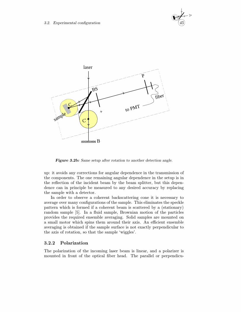
Figure 3.2b: Same setup after rotation to another detection angle.
up: it avoids any corrections for angular dependence in the transmission ofthe components. The one remaining angular dependence in the setup is inthe reflection of the incident beam by the beam splitter, but this depen-dence can in principle be measured to any desired accuracy by replacingthe sample with a detector.
In order to observe a coherent backscattering cone it is necessary toaverage over many configurations of the sample. This eliminates the specklepattern which is formed if a coherent beam is scattered by a (stationary)random sample [5]. In a fluid sample, Brownian motion of the particlesprovides the required ensemble averaging. Solid samples are mounted ona small motor which spins them around their axis. An efficient ensembleaveraging is obtained if the sample surface is not exactly perpendicular tothe axis of rotation, so that the sample ‘wiggles’.
3.2.2 Polarization
The polarization of the incoming laser beam is linear, and a polarizer ismounted in front of the optical fiber head. The parallel or perpendicu-
46 An accurate technique to record coherent backscattering
lar polarization channel in the scattered light is selected by means of thispolarizer. If experiments with circularly polarized incident light are de-sired, a quarter-wave plate is mounted in front of the sample to convert theincoming linear polarization to circular polarization. The two circular com-ponents of the outgoing scattered light are converted back by this quarterwaveplate to mutually perpendicular linear components. The polarizer infront of the fiber is used in that case to select the linear polarization thatcorresponds to either one of the helicity channels of the scattered light.
A setup with two quarter waveplates, where one is placed in the incidentbeam and one in front of the detector, in not possible for the followingreason. The reflection coefficient of the beam splitter depends both on theangle and on the polarization. An incoming circular polarization wouldbecome elliptical after reflection on the beamsplitter, and the ellipticitywould be angle-dependent. This is why one waveplate is mounted in frontof the sample. The incident and scattered waves will pass this quarterwaveplate under necessarily different angles. Since only at perpendicularincidence the relative phase shift corresponds to exactly a quarter of awave, some mixing of polarizations will occur in directions that are farfrom exact backscattering. We used a zero order quarter waveplate becauseits angular tolerance is far greater than that of a multi order one. Wefound that even at the largest angles studied, the intensity coupled intothe opposite polarization channel remained < 1%. In directions far fromexact backscattering, our random samples scramble the polarization almostcompletely. Errors from mixing of polarization due to oblique incidence inthe quarter waveplate, will therefore essentially cancel. We estimate theoverall error in the measured curves due to oblique incidence in the quarterwaveplate to be < 0.1%.
3.2.3 Angular resolution and scanning range
The scanning range of the setup is determined by the size of the beamsplitter. We have used a beam splitter of 5 cm diameter and an incomingbeam diameter of 5 mm, and obtained a scanning range of about 500 mrad.The angular resolution of the setup was diffraction limited by the diameterd of the incident beam. With d = 5 mm and using visible light, this limitis ≈ 100 µrad. The detection optics (50 µm core fiber, with its tip at a 1m distance from the sample) allows in principle a resolution of 50 µrad.
3.2. Experimental configuration 47
beamsplitter
window
sample
incoming beam
screen
a
c
b
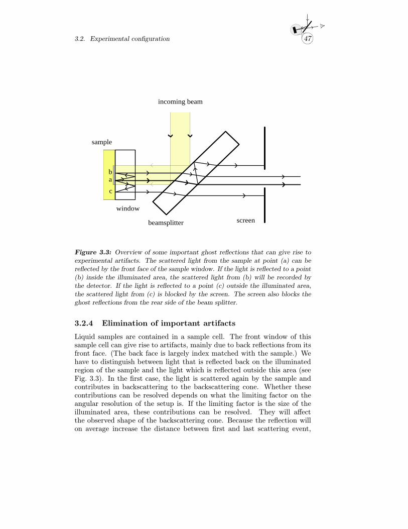
Figure 3.3: Overview of some important ghost reflections that can give rise to
experimental artifacts. The scattered light from the sample at point (a) can be
reflected by the front face of the sample window. If the light is reflected to a point
(b) inside the illuminated area, the scattered light from (b) will be recorded by
the detector. If the light is reflected to a point (c) outside the illuminated area,
the scattered light from (c) is blocked by the screen. The screen also blocks the
ghost reflections from the rear side of the beam splitter.
3.2.4 Elimination of important artifacts
Liquid samples are contained in a sample cell. The front window of thissample cell can give rise to artifacts, mainly due to back reflections from itsfront face. (The back face is largely index matched with the sample.) Wehave to distinguish between light that is reflected back on the illuminatedregion of the sample and the light which is reflected outside this area (seeFig. 3.3). In the first case, the light is scattered again by the sample andcontributes in backscattering to the backscattering cone. Whether thesecontributions can be resolved depends on what the limiting factor on theangular resolution of the setup is. If the limiting factor is the size of theilluminated area, these contributions can be resolved. They will affectthe observed shape of the backscattering cone. Because the reflection willon average increase the distance between first and last scattering event,
48 An accurate technique to record coherent backscattering
the cone will become narrower. If the angular resolution is lower, thesecontributions can not be (fully) resolved, and will lead to a lowering ofthe observed enhancement factor. The light that is reflected by the frontwindow surface to regions outside the illuminated area can not contributeto the backscattering cone because these waves have no counterpropagatingcounterparts. This light will however contribute to the background and willtherefore also lower the observed enhancement factor.
To reduce the above effects, the glass window must be thick (1 cm) andits front side must be anti-reflection coated. Moreover, the second effectcan be eliminated by placing a diaphragm between the beam splitter andthe positive lens. The aperture of this diaphragm is only slightly largerthan the illuminated region on the sample. It is aligned such that onlyscattered light from the illuminated region can reach the detector. Notethat this solution is possible because in our setup the light path from sampleto detector is always the same. This property of the setup also allows toshield other sources of stray light in a convenient way without the risk ofpartly masking the field of view of the detector during part of an angularscan (‘clipping’).
A glass window can also be used to index match the front interfaceof a rigid sample, in order to eliminate internal reflection [6]. The sameconsiderations hold as for the front window of a liquid sample cell. Greatcare has to be taken to ensure a good optical contact between window andsample surface. We obtained good results if we coated the rear side of theglass window with collodium and pressed this side with force on the sample.
The beam splitter is a slightly wedged thick window with a 50 % re-flectance coating on the front side and an anti-reflection coating on the backside. All (multiple) reflections that arise from the small remaining reflectionof the back surface will be blocked by the diaphragm placed between beamsplitter and positive lens if the beam splitter is sufficiently thick (about1cm). Due to its wedged shape, etalon effects in the beam splitter are alsoavoided.
3.2.5 Response of the setup
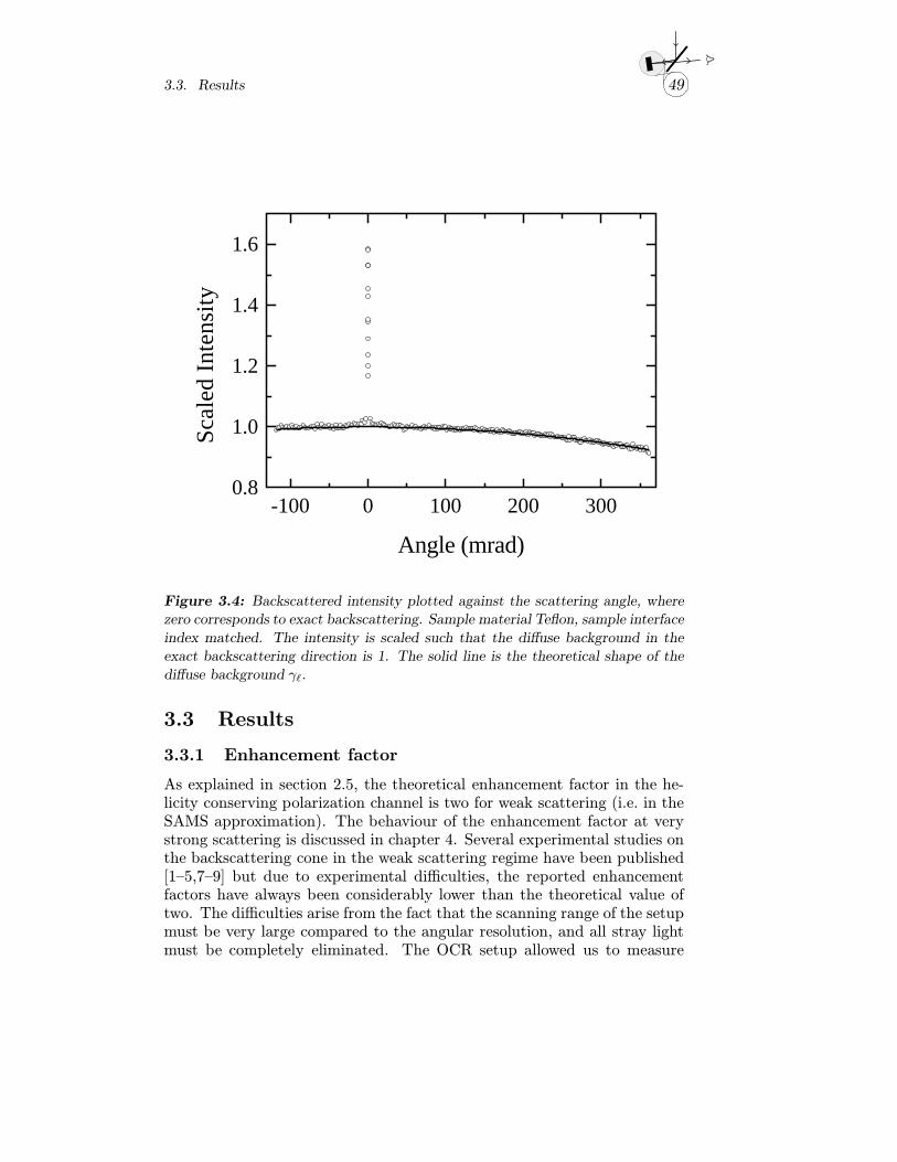
To check the response of the setup over a large angular range, we haverecorded the backscattering from a very weakly scattering sample (i.e. asample with a very large mean free path) (see Fig. 3.4). The backscatteringcone of this (teflon) sample is extremely narrow so the major part of thescan yields the (almost angle-independent) diffuse background. The solidline in Fig. 3.4 is the diffuse background in the diffusion approximation[given by Eq. (2.50)]. Agreement between data and theory is very good.
3.3. Results 49
-100 0 100 200 3000.8
1.0
1.2
1.4
1.6
Sca
led
Inte
nsit
y
Angle (mrad)
Figure 3.4: Backscattered intensity plotted against the scattering angle, where
zero corresponds to exact backscattering. Sample material Teflon, sample interface
index matched. The intensity is scaled such that the diffuse background in the
exact backscattering direction is 1. The solid line is the theoretical shape of the
diffuse background γ�.
3.3 Results
3.3.1 Enhancement factor
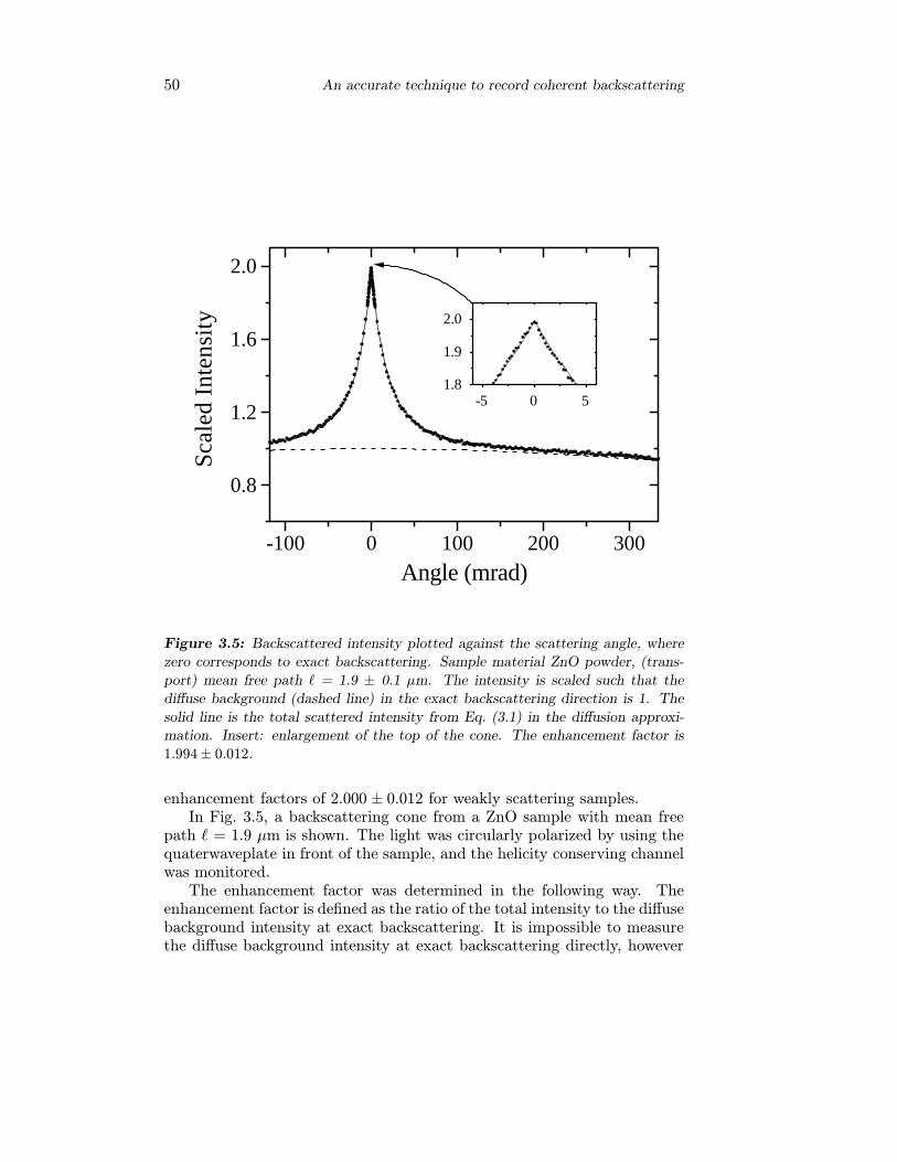
As explained in section 2.5, the theoretical enhancement factor in the he-licity conserving polarization channel is two for weak scattering (i.e. in theSAMS approximation). The behaviour of the enhancement factor at verystrong scattering is discussed in chapter 4. Several experimental studies onthe backscattering cone in the weak scattering regime have been published[1–5,7–9] but due to experimental difficulties, the reported enhancementfactors have always been considerably lower than the theoretical value oftwo. The difficulties arise from the fact that the scanning range of the setupmust be very large compared to the angular resolution, and all stray lightmust be completely eliminated. The OCR setup allowed us to measure
50 An accurate technique to record coherent backscattering
-100 0 100 200 300
0.8
1.2
1.6
2.0
Sca
led
Inte
nsit
y
Angle (mrad)
-5 0 51.8
1.9
2.0
Figure 3.5: Backscattered intensity plotted against the scattering angle, where
zero corresponds to exact backscattering. Sample material ZnO powder, (trans-
port) mean free path = 1.9 ± 0.1 µm. The intensity is scaled such that the
diffuse background (dashed line) in the exact backscattering direction is 1. The
solid line is the total scattered intensity from Eq. (3.1) in the diffusion approxi-
mation. Insert: enlargement of the top of the cone. The enhancement factor is
1.994± 0.012.
enhancement factors of 2.000 ± 0.012 for weakly scattering samples.In Fig. 3.5, a backscattering cone from a ZnO sample with mean free
path = 1.9 µm is shown. The light was circularly polarized by using thequaterwaveplate in front of the sample, and the helicity conserving channelwas monitored.
The enhancement factor was determined in the following way. Theenhancement factor is defined as the ratio of the total intensity to the diffusebackground intensity at exact backscattering. It is impossible to measurethe diffuse background intensity at exact backscattering directly, however
3.3. Results 51
the diffuse background is largely angle-independent over the angular extendof the backscattering cone. One can determine the enhancement factor bycomparing the data with a theoretical expression for the total intensity thatallows for extra background contributions from experimental artifacts:
I(θ) = a0[γc(θ) + (1 + ε)γ�(θ)]. (3.1)
Here a0 is a normalization factor, and ε >∼ 0 determines the contribution tothe background intensity due to artifacts, where it is assumed that thesecontributions have the same angular dependence as γ�. The enhancementfactor is then given by:
E =γc + (1 + ε)γ�
(1 + ε)γ�
∣∣∣∣θ=0
=2 + ε
1 + ε, (3.2)
where ε is determined from the data. Note that in order to determine εaccurately, the scanning range must be large enough to cover at least thewings of the cone where γc is almost zero.
We have determined the enhancement factor for various measurementsfrom samples in the weak scattering regime. The samples are suspensionsof TiO2 in 2-methylpentane 2,4-diol and powders of ZnO or BaSO4. Thelight was circular polarized and the wavelength was either 514.0 nm or632.8 nm. The results are shown in Table 3.1. The enhancement factor forall measurements is in the range 2.000 ± 0.012. The mean free path wasdetermined from the width of the cone using equation 2.56.
3.3.2 The shape of the backscattering cone
As can be seen from Fig. 3.5, the shape of the backscattering cone agreesvery well with the backscattering cone calculated in the diffusion ap-proximation. The intensity propagator F (r1, r2) needed to calculate thebackscattering cone can also be found without making the diffusion ap-proximation, either numerically for a finite slab [8,9] or analytically for asemi-infinite slab geometry [10]. This leads to a solution for the backscatter-ing cone that is exact for scalar waves, but which not necessarily describesthe backscattering cone for light better than the diffusion approximation.Firstly, light waves are vector waves. Secondly, the exact calculation as-sumes point scatterers whereas the real physical scatterers are irregularly
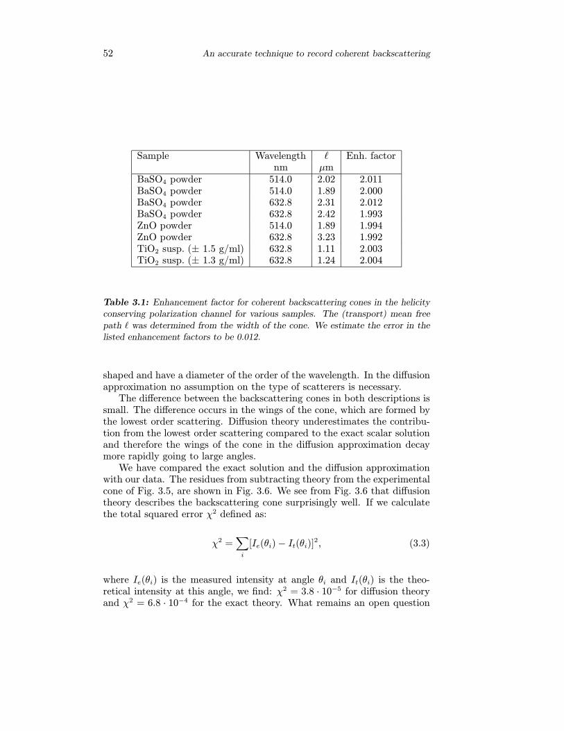
52 An accurate technique to record coherent backscattering
Sample Wavelength Enh. factornm µm
BaSO4 powder 514.0 2.02 2.011BaSO4 powder 514.0 1.89 2.000BaSO4 powder 632.8 2.31 2.012BaSO4 powder 632.8 2.42 1.993ZnO powder 514.0 1.89 1.994ZnO powder 632.8 3.23 1.992TiO2 susp. (± 1.5 g/ml) 632.8 1.11 2.003TiO2 susp. (± 1.3 g/ml) 632.8 1.24 2.004
Table 3.1: Enhancement factor for coherent backscattering cones in the helicity
conserving polarization channel for various samples. The (transport) mean free
path was determined from the width of the cone. We estimate the error in the
listed enhancement factors to be 0.012.
shaped and have a diameter of the order of the wavelength. In the diffusionapproximation no assumption on the type of scatterers is necessary.
The difference between the backscattering cones in both descriptions issmall. The difference occurs in the wings of the cone, which are formed bythe lowest order scattering. Diffusion theory underestimates the contribu-tion from the lowest order scattering compared to the exact scalar solutionand therefore the wings of the cone in the diffusion approximation decaymore rapidly going to large angles.
We have compared the exact solution and the diffusion approximationwith our data. The residues from subtracting theory from the experimentalcone of Fig. 3.5, are shown in Fig. 3.6. We see from Fig. 3.6 that diffusiontheory describes the backscattering cone surprisingly well. If we calculatethe total squared error χ2 defined as:
χ2 =∑i
[Ie(θi)− It(θi)]2, (3.3)
where Ie(θi) is the measured intensity at angle θi and It(θi) is the theo-retical intensity at this angle, we find: χ2 = 3.8 · 10−5 for diffusion theoryand χ2 = 6.8 · 10−4 for the exact theory. What remains an open question
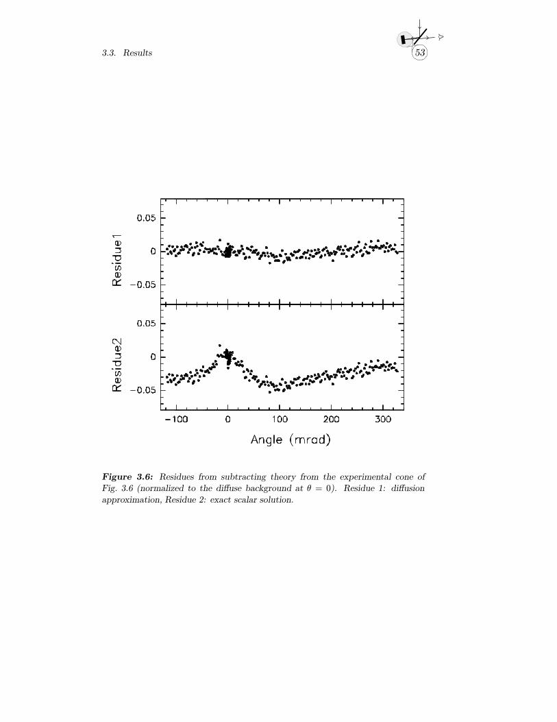
3.3. Results 53
Figure 3.6: Residues from subtracting theory from the experimental cone of
Fig. 3.6 (normalized to the diffuse background at θ = 0). Residue 1: diffusion
approximation, Residue 2: exact scalar solution.
54 An accurate technique to record coherent backscattering
is why the diffusion approximation corresponds better with the data thanthe exact solution. A possible explanation lies in the polarization characterof light which is not taken into account in either theory. For the lower or-der scattering, less light is scattered in the helicity conserving than in thehelicity reversing polarization channel, whereas for the higher orders the po-larization is completely scrambled. Therefore, the lower order contributionsin the helicity conserving polarization channel are less important than anexact scalar theory predicts. The diffusion approximation underestimatesthe contribution from the lowest orders compared to the exact solution andthis apparantly results in a better description of the backscattering cone.

55
References and notes
[1] M. Kaveh, M. Rosenbluh, I. Edrei, and I. Freund, Phys. Rev. Lett. 57,2049 (1986).
[2] M. Rosenbluh, I. Edrei, M. Kaveh, and I. Freund, Phys. Rev. A 35,4458 (1987).
[3] M.P. van Albada and A. Lagendijk, Phys. Rev. Lett. 55, 2692 (1985).[4] P.E. Wolf and G. Maret, Phys. Rev. Lett. 55, 2696 (1985).[5] S. Etemad, R. Thompson, and M.J. Andrejco, Phys. Rev. Lett. 57,
575 (1986).[6] A. Lagendijk, B. Vreeker, and P. de Vries, Phys. Lett. A 136, 81 (1989);
J.X. Zhu, D.J. Pine, and D.A. Weitz, Phys. Rev. A 44, 3948 (1991);Th.M. Nieuwenhuizen and J.M. Luck, Phys. Rev. E 48, 569 (1993).
[7] Y. Kuga and A. Ishimaru, J. Opt. Soc. Am. A 8, 831 (1984).[8] M.B. van der Mark, M.P. van Albada, and A. Lagendijk, Phys. Rev.
B 37, 3575 (1988).[9] P.E. Wolf, G. Maret, E. Akkermans, and R. Maynard, J. Phys. France
49, 63 (1988).[10] E.E. Gorodnichev, S.L. Dudarev, and D.B. Rogozkin, Phys. Lett. A
144, 48 (1990).

56
Chapter 4
Experimental evidence forrecurrent multiple scattering
4.1 Introduction
In chapter 2, an introduction is given to the theory which is commonlyused to treat multiple light scattering in disordered media. The presentedderivations are valid for relatively weakly scattering media, because recur-rent scattering is neglected. Recurrent scattering events are events in whicha wave is scattered by a specific scatterer, scattered by at least one otherscatterer and then returns to this specific scatterer. For relatively weakscattering, recurrent events can be neglected, because the chance of a wavereturning to a specific scatterer is very small. This approximation is calledthe ‘self-avoiding multiple scattering’ (SAMS) approximation. In most ex-perimental studies that have been published so far, the scattering was weakenough to neglect recurrent scattering.
To explain the relevance of recurrent scattering, a parallel can be drawnto electron scattering. It is known that the propagation of electrons ina disordered structure can change tremendously in the strong scatteringregime. Below a critical value of the electron scattering mean free path,the diffusion of the electrons can disappear. This phenomenon is knownas Anderson localization [1]. The propagation of light in disordered di-electrics shows interesting similarities to electron transport in disordered(semi-)conductors [2], and it is challenging to find an optical counterpartof Anderson localization. Recurrent scattering plays an important role inthe theory of Anderson localization [3,4]. The reduction of the diffusionconstant can be explained by constructive interference between waves that
57
58 Experimental evidence for recurrent multiple scattering
have propagated along the same path in opposite directions. Due to thisconstructive interference, the probability for a wave to return to a specificscatterer increases and thereby the probability to propagate away from thisscatterer decreases. So far however, no experimental evidence was presentfor the existence of recurrent scattering of light waves in disordered media.
A parameter which is a measure for the scattering strength is (k s)−1,
where s is the scattering mean free path and k is the wavenumber of thelight in the medium. If Anderson localization of light is possible, it isexpected to occur at very strong scattering, that is for very small k s. Forelectrons, a localized state is obtained at k s < 1. This criterion is knownas the Ioffe-Regel criterion [5]. For light it is very difficult to obtain samplesin the regime k s < 1 (see section 1.1.3). However it is possible to get closeto k s = 1, where effects from recurrent scattering might already be visible.
In this chapter, we will study coherent backscattering from stronglyscattering media, to find evidence for recurrent scattering of light waves.The relevant parameter in these experiments is the enhancement factor ofthe backscattering cone, which is the ratio of the total scattered intensityat exact backscattering to the diffuse background. As explained in sec-tion 2.5.1, the enhancement factor is two in the weak scattering regime, ifthe single scattering contribution is eliminated. Single scattering lowers theenhancement factor because it does not contribute an interference term. Ina single scattering event, a wave enters and leaves the sample on the samescatterer. If recurrent scattering occurs, we expect the subclass of recurrentevents in which first and last scattering occurs on the same scatterer, to be-have similar to single scattering (see Fig. 4.1). One can distinguish betweenthese recurrent events and single scattering, by using circularly polarizedlight and monitoring the helicity conserving polarization channel. Singlescattering will not be present in the helicity conserving channel using spher-ical symmetric scatterers, whereas for recurrent scattering the polarizationwill be (at least partly) scrambled. This means we have to measure theenhancement factor in the helicity conserving channel as a function of thescattering strength, where deviations from two close to k s = 1 would be amanifestation of recurrent scattering.
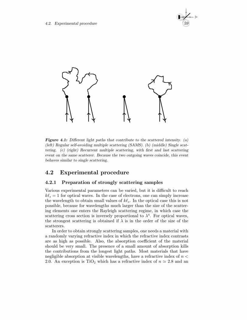
4.2. Experimental procedure 59
Figure 4.1: Different light paths that contribute to the scattered intensity. (a)
(left) Regular self-avoiding multiple scattering (SAMS). (b) (middle) Single scat-
tering. (c) (right) Recurrent multiple scattering, with first and last scattering
event on the same scatterer. Because the two outgoing waves coincide, this event
behaves similar to single scattering.
4.2 Experimental procedure
4.2.1 Preparation of strongly scattering samples
Various experimental parameters can be varied, but it is difficult to reachk s = 1 for optical waves. In the case of electrons, one can simply increasethe wavelength to obtain small values of k s. In the optical case this is notpossible, because for wavelengths much larger than the size of the scatter-ing elements one enters the Rayleigh scattering regime, in which case thescattering cross section is inversely proportional to λ4. For optical waves,the strongest scattering is obtained if λ is in the order of the size of thescatterers.
In order to obtain strongly scattering samples, one needs a material witha randomly varying refractive index in which the refractive index contrastsare as high as possible. Also, the absorption coefficient of the materialshould be very small. The presence of a small amount of absorption killsthe contributions from the longest light paths. Most materials that havenegligible absorption at visible wavelengths, have a refractive index of n <2.0. An exception is TiO2 which has a refractive index of n 2.8 and an
60 Experimental evidence for recurrent multiple scattering
absorption coefficient of κi 10 mm−1 at λvac = 514 nm. Various powdersbased on TiO2 are used as pigments in the paint industry because of theirstrong scattering properties.
We have used a powder of rutile TiO2 microparticles that was treatedwith SiO2, Al2O3, and organical compounds to prevent the particles fromclustering [6]. The diameter of the particles in this powder is in the rangeof 100 nm to 300 nm. The powder was suspended in chloroform and groundin a planetary micro mill for about 1 minute to break possible clusters. Wefound that milling times longer than 5 minutes are undesirable because after5 minutes the particles start to cluster, possibly because their coating isremoved (see Fig. 4.2). After grinding, the chloroform was left to evaporate.This way, samples could be obtained with k s 6 at λvac = 514 nm.
Other values of k s were obtained by varying the sample material andwavelength. Apart from TiO2, also ZnO (n = 2.0) and BaSO4 (n = 1.6)were used. The latter is available as a diffuse reflectance coating [7]. Apartfrom the refractive index of the scatterers themselves, the refractive indexof the surrounding medium was varied as well, by suspending the TiO2particles either in methylpentanediol (n = 1.43) or in methanol (n = 1.33).
4.2.2 Enhancement factor in coherent backscattering
We have recorded backscattering cones from the various strongly scatter-ing samples, using the ‘off-centered rotation’ setup described in chapter 3.Great care was taken in recording the backscattering cones accurately asmany experimental artifacts also result in an enhancement factor smal-ler than two. With the setup described in chapter 3, it was possible todetermine the enhancement factor in a reliable way and with the desiredaccuracy.
The procedure of determining the enhancement factor is essentially thesame as described in section 3.3.1. We allow for extra contributions to theintensity from recurrent events where we make the realistic assumptionsthat (a) these contributions have the same angular dependence as γ� and(b) the shape of the backscattering cone remains the same. So we compareour data to the theoretical intensity given by:
I(θ) = a0[γc(θ) + (1 + ε)γ�(θ)], (4.1)
where a0 is a normalization factor and ε is the relative contribution of
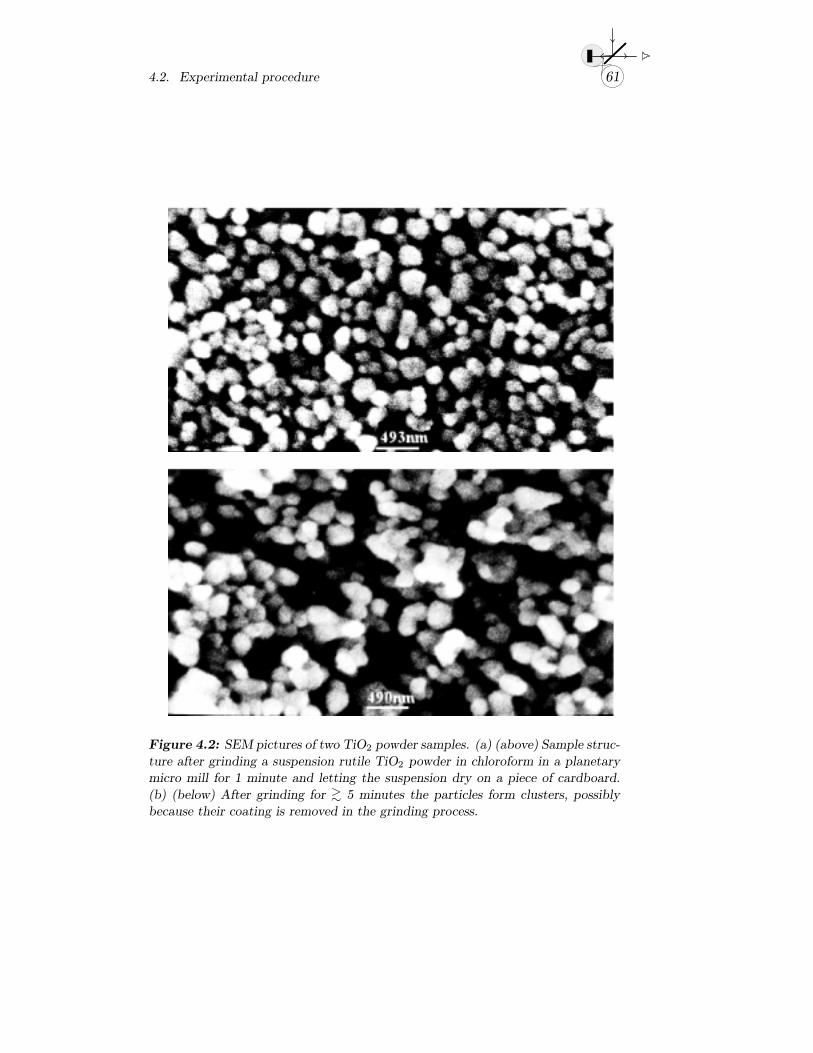
4.2. Experimental procedure 61
Figure 4.2: SEM pictures of two TiO2 powder samples. (a) (above) Sample struc-
ture after grinding a suspension rutile TiO2 powder in chloroform in a planetary
micro mill for 1 minute and letting the suspension dry on a piece of cardboard.
(b) (below) After grinding for >∼ 5 minutes the particles form clusters, possibly
because their coating is removed in the grinding process.
62 Experimental evidence for recurrent multiple scattering
recurrent events. The enhancement factor E in terms of ε is then given by:
E =γc + (1 + ε)γ�
(1 + ε)γ�
∣∣∣∣θ=0
=2 + ε
1 + ε. (4.2)
For γ� and γc, we take the the bistatic coefficients for weak scattering cal-culated in the diffusion approximation [Eqs. (2.50) and (2.54)]. As we haveshown in section 3.3.2, both the diffuse background and the backscatteringcone in the helicity conserving channel are very well described by diffusiontheory.
The enhancement factor was determined by fitting the backscatteringcone of Eq. (4.1) to the data with ε, a0, and the cone width W [8] theadjustable parameters. We found that this procedure gives reliable valuesfor the enhancement factor provided that the scanning range is so largethat the wings of the cone are almost completely covered. It is important toknow the intensity in the wings because the ratio of top to wings determinesE. We have checked our method of determining E in different ways. Toverify whether the results do not critically depend on the precise theoreticalcone shape, we have used for γc the exact solution for scalar waves [9]instead of the diffusion approximation. In that case, the correspondencebetween experimental data and theoretical backscattering cone is not asgood as when using diffusion theory, but the behaviour of the enhancementfactor versus k s remains the same. We also tried to fit all our resultsforcing E = 2 and keeping the other parameters free. In that case, themean squared error of the fit remains essentially the same at large W−1,whereas at small W−1, the theoretical cone systematically deviates fromthe data and the mean squared error becomes larger by a factor >∼ 4.
4.2.3 Determination of the mean free path
The mean free path can be found in principle from the width of the coneusing Eq. (2.56): W = (0.7/2π)(λe/ ), where λe is the wavelength in themedium between the sample and the detector (air). However, this expres-sion does not incorporate effects from internal reflection by the refractiveindex contrast at the front sample interface. Internal reflection reducesthe width of the backscattering cone [10], so if we wish to infer fromthe width of the cone, we either have to eliminate internal reflection or wehave to estimate how large the effect is and compensate for it. We havepursued both options in our experiments, in order to be able to comparethe results. Internal reflection was eliminated for some samples by index
4.3. Results 63
matching the sample interface with a thick (1 cm) glass window. For thenon index matched samples we generalize Eq. (2.56) to [10]:
W ξ0.7
2π
λe , (4.3)
where ξ must be calculated from the average refractive index of the sample,as is done in the next section.
4.3 Results
An example of two backscattering cones is shown in Fig. 4.3. The broadcone corresponds to a sample with a very small mean free path (k s =5.8 ± 1.0), while the narrow cone corresponds to a sample in the weakscattering regime. As we can see from the inset, the enhancement factor inthe measurement on the stronger scattering sample, is smaller than two.
We have recorded various backscattering cones from the TiO2, ZnO andBaSO4 powders and from the suspensions of TiO2 in methylpentanediol andmethanol. Most samples were prepared both with an index matched andwith a non index matched interface. The measurements were performed attwo wavelengths: 514 nm and 633 nm, and the helicity conserving channelwas monitored. For all measurements, the enhancement factor was deter-mined as a function of the inverse cone width W−1, which is plotted inFig. 4.4. The two classes of measurements, one with an index matched andone with a non index matched sample interface, are shown separately. Inboth series the enhancement factor is 2.00 ± 0.01 for large W−1 and dropsbelow 2.00 for very small W−1, which corresponds to very short mean freepaths.
4.3.1 Enhancement factor versus mean free path
As we are interested in the functional dependence of E on the k s, we haveto calculate s from the cone widthW . For the index matched series we cansimply use Eq. (4.3) with ξ = 1, assuming isotropic scattering ( s = ) [11].For the non index matched series, we have to estimate ξ. The reflectivityR of the sample interface depends on the refractive index contrast at theboundary. The bulk refractive index (nmed) of a collection of particles withrefractive index n2 in a surrounding medium with refractive index n1 (wheren1 < n2), is generally much lower than the weighted average of n1 and n2[12]. For the 35 vol% TiO2-air samples, it is estimated to be 1.35 ± 0.10,
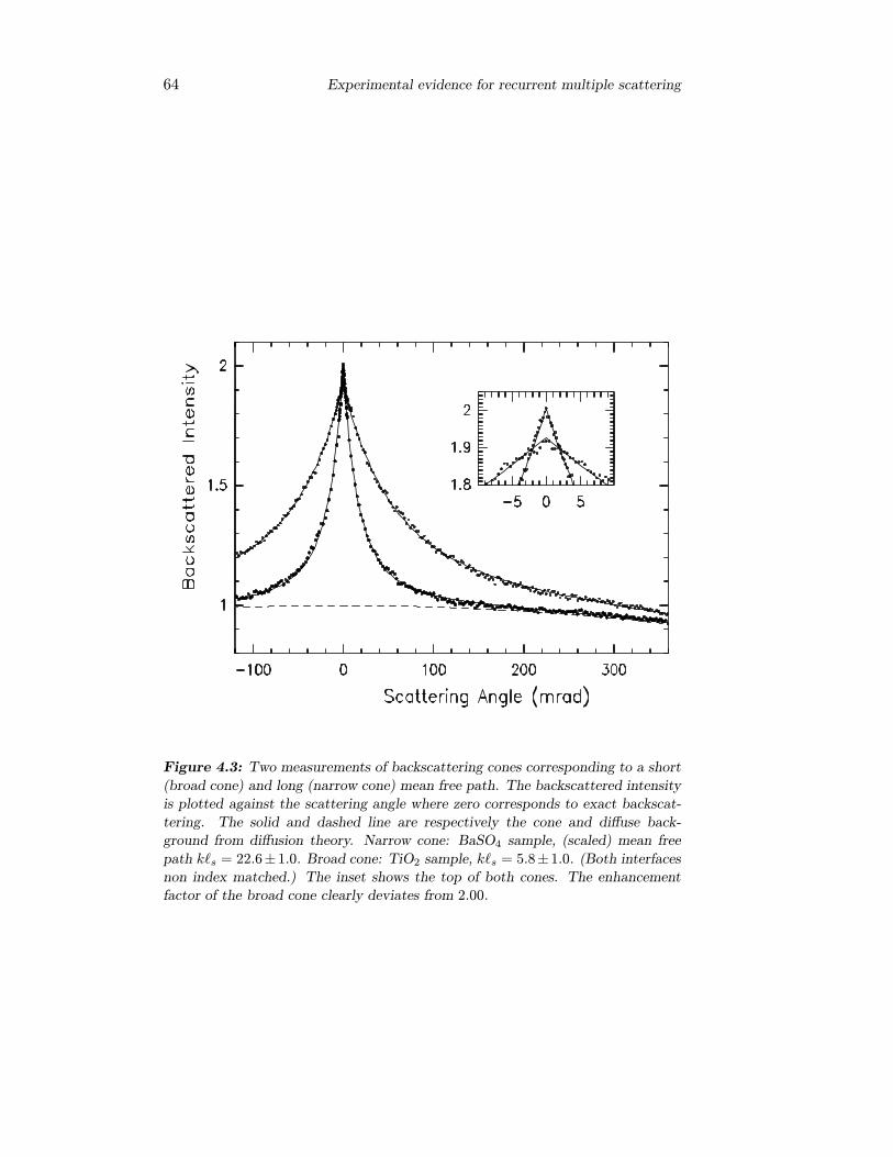
64 Experimental evidence for recurrent multiple scattering
Figure 4.3: Two measurements of backscattering cones corresponding to a short
(broad cone) and long (narrow cone) mean free path. The backscattered intensity
is plotted against the scattering angle where zero corresponds to exact backscat-
tering. The solid and dashed line are respectively the cone and diffuse back-
ground from diffusion theory. Narrow cone: BaSO4 sample, (scaled) mean free
path k s = 22.6±1.0. Broad cone: TiO2 sample, k s = 5.8±1.0. (Both interfaces
non index matched.) The inset shows the top of both cones. The enhancement
factor of the broad cone clearly deviates from 2.00.
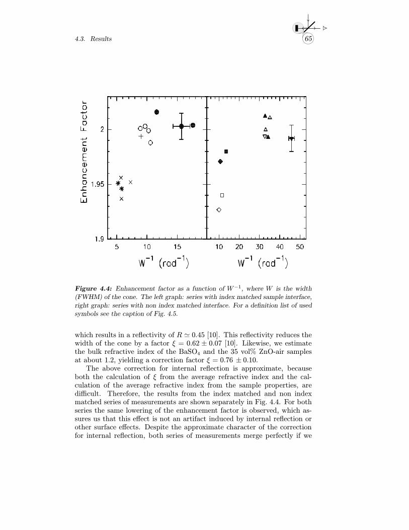
4.3. Results 65
Figure 4.4: Enhancement factor as a function of W−1, where W is the width
(FWHM) of the cone. The left graph: series with index matched sample interface,
right graph: series with non index matched interface. For a definition list of used
symbols see the caption of Fig. 4.5.
which results in a reflectivity of R 0.45 [10]. This reflectivity reduces thewidth of the cone by a factor ξ = 0.62 ± 0.07 [10]. Likewise, we estimatethe bulk refractive index of the BaSO4 and the 35 vol% ZnO-air samplesat about 1.2, yielding a correction factor ξ = 0.76 ± 0.10.
The above correction for internal reflection is approximate, becauseboth the calculation of ξ from the average refractive index and the cal-culation of the average refractive index from the sample properties, aredifficult. Therefore, the results from the index matched and non indexmatched series of measurements are shown separately in Fig. 4.4. For bothseries the same lowering of the enhancement factor is observed, which as-sures us that this effect is not an artifact induced by internal reflection orother surface effects. Despite the approximate character of the correctionfor internal reflection, both series of measurements merge perfectly if we
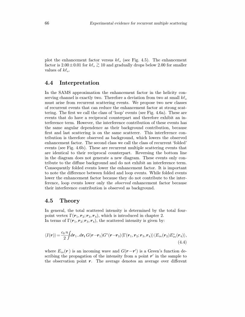
66 Experimental evidence for recurrent multiple scattering
plot the enhancement factor versus k s (see Fig. 4.5). The enhancementfactor is 2.00±0.01 for k s >∼ 10 and gradually drops below 2.00 for smallervalues of k s.
4.4 Interpretation
In the SAMS approximation the enhancement factor in the helicity con-serving channel is exactly two. Therefore a deviation from two at small k smust arise from recurrent scattering events. We propose two new classesof recurrent events that can reduce the enhancement factor at strong scat-tering. The first we call the class of ‘loop’ events (see Fig. 4.6a). These areevents that do have a reciprocal counterpart and therefore exhibit an in-terference term. However, the interference contribution of these events hasthe same angular dependence as their background contribution, becausefirst and last scattering is on the same scatterer. This interference con-tribution is therefore observed as background, which lowers the observedenhancement factor. The second class we call the class of recurrent ‘folded’events (see Fig. 4.6b). These are recurrent multiple scattering events thatare identical to their reciprocal counterpart. Reversing the bottom linein the diagram does not generate a new diagram. These events only con-tribute to the diffuse background and do not exhibit an interference term.Consequently folded events lower the enhancement factor. It is importantto note the difference between folded and loop events. While folded eventslower the enhancement factor because they do not contribute to the inter-ference, loop events lower only the observed enhancement factor becausetheir interference contribution is observed as background.
4.5 Theory
In general, the total scattered intensity is determined by the total four-point vertex Γ(r1, r2; r3, r4), which is introduced in chapter 2.In terms of Γ(r1, r2; r3, r4), the scattered intensity is given by:
〈I(r)〉=c0 n
2
∫dr1..dr4G(r−r1)G
∗(r−r3)〈Γ(r1, r2; r3, r4)〉〈Ein(r2)E∗in(r4)〉,
(4.4)
where Ein(r ) is an incoming wave and G(r−r′) is a Green’s function de-scribing the propagation of the intensity from a point r′ in the sample tothe observation point r. The average denotes an average over different
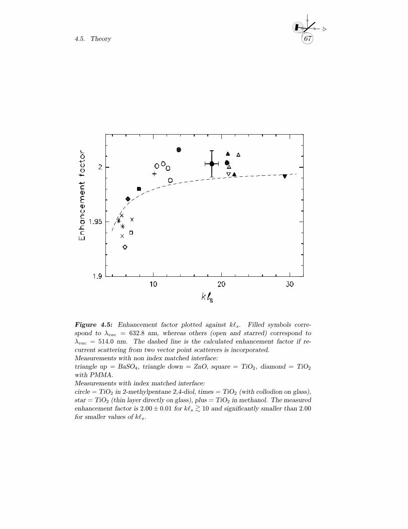
4.5. Theory 67
Figure 4.5: Enhancement factor plotted against k s. Filled symbols corre-
spond to λvac = 632.8 nm, whereas others (open and starred) correspond to
λvac = 514.0 nm. The dashed line is the calculated enhancement factor if re-
current scattering from two vector point scatterers is incorporated.
Measurements with non index matched interface:
triangle up = BaSO4, triangle down = ZnO, square = TiO2, diamond = TiO2with PMMA.
Measurements with index matched interface:
circle = TiO2 in 2-methylpentane 2,4-diol, times = TiO2 (with collodion on glass),
star = TiO2 (thin layer directly on glass), plus = TiO2 in methanol. The measured
enhancement factor is 2.00± 0.01 for k s >∼ 10 and significantly smaller than 2.00
for smaller values of k s.
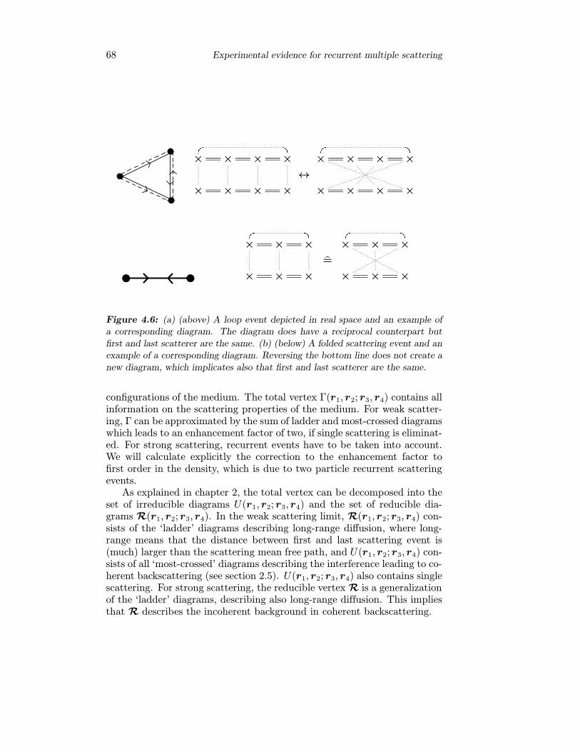
68 Experimental evidence for recurrent multiple scattering
×'& %$
× × ×
× × × ×
↔
×'& %$
× × ×
× × × ×
×'& %$
× ×
× × ×
=
×'& %$
× ×
× × ×
Figure 4.6: (a) (above) A loop event depicted in real space and an example of
a corresponding diagram. The diagram does have a reciprocal counterpart but
first and last scatterer are the same. (b) (below) A folded scattering event and an
example of a corresponding diagram. Reversing the bottom line does not create a
new diagram, which implicates also that first and last scatterer are the same.
configurations of the medium. The total vertex Γ(r1, r2; r3, r4) contains allinformation on the scattering properties of the medium. For weak scatter-ing, Γ can be approximated by the sum of ladder and most-crossed diagramswhich leads to an enhancement factor of two, if single scattering is eliminat-ed. For strong scattering, recurrent events have to be taken into account.We will calculate explicitly the correction to the enhancement factor tofirst order in the density, which is due to two particle recurrent scatteringevents.
As explained in chapter 2, the total vertex can be decomposed into theset of irreducible diagrams U(r1, r2; r3, r4) and the set of reducible dia-grams R(r1, r2; r3, r4). In the weak scattering limit, R(r1, r2; r3, r4) con-sists of the ‘ladder’ diagrams describing long-range diffusion, where long-range means that the distance between first and last scattering event is(much) larger than the scattering mean free path, and U(r1, r2; r3, r4) con-sists of all ‘most-crossed’ diagrams describing the interference leading to co-herent backscattering (see section 2.5). U(r1, r2; r3, r4) also contains singlescattering. For strong scattering, the reducible vertexR is a generalizationof the ‘ladder’ diagrams, describing also long-range diffusion. This impliesthat R describes the incoherent background in coherent backscattering.
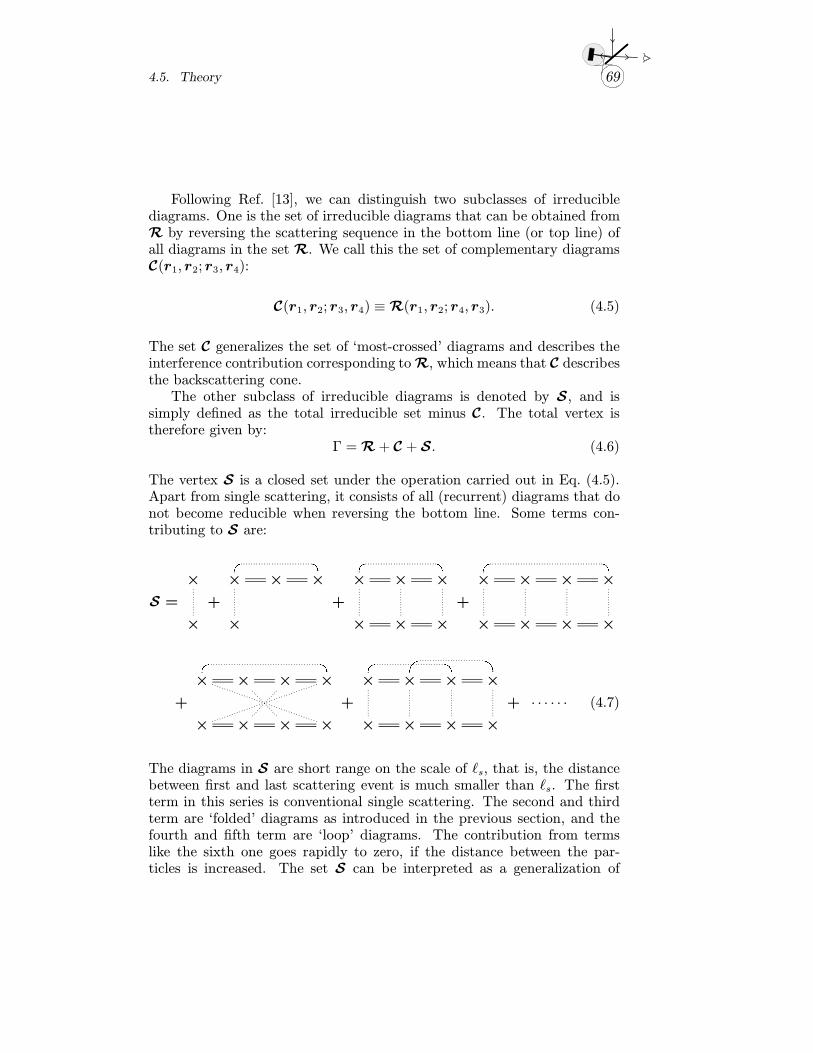
4.5. Theory 69
Following Ref. [13], we can distinguish two subclasses of irreduciblediagrams. One is the set of irreducible diagrams that can be obtained fromR by reversing the scattering sequence in the bottom line (or top line) ofall diagrams in the set R. We call this the set of complementary diagramsC(r1, r2; r3, r4):
C(r1, r2; r3, r4) ≡R(r1, r2; r4, r3). (4.5)
The set C generalizes the set of ‘most-crossed’ diagrams and describes theinterference contribution corresponding toR, which means that C describesthe backscattering cone.
The other subclass of irreducible diagrams is denoted by S, and issimply defined as the total irreducible set minus C. The total vertex istherefore given by:
Γ =R+ C + S. (4.6)
The vertex S is a closed set under the operation carried out in Eq. (4.5).Apart from single scattering, it consists of all (recurrent) diagrams that donot become reducible when reversing the bottom line. Some terms con-tributing to S are:
S =
×
×
+
×'& %$
× ×
×
+
×'& %$
× ×
× × ×
+
×'& %$
× × ×
× × × ×
+
×'& %$
× × ×
× × × ×
+
×'& %$
×?> =<
× ×
× × × ×
+ · · · · · · (4.7)
The diagrams in S are short range on the scale of s, that is, the distancebetween first and last scattering event is much smaller than s. The firstterm in this series is conventional single scattering. The second and thirdterm are ‘folded’ diagrams as introduced in the previous section, and thefourth and fifth term are ‘loop’ diagrams. The contribution from termslike the sixth one goes rapidly to zero, if the distance between the par-ticles is increased. The set S can be interpreted as a generalization of
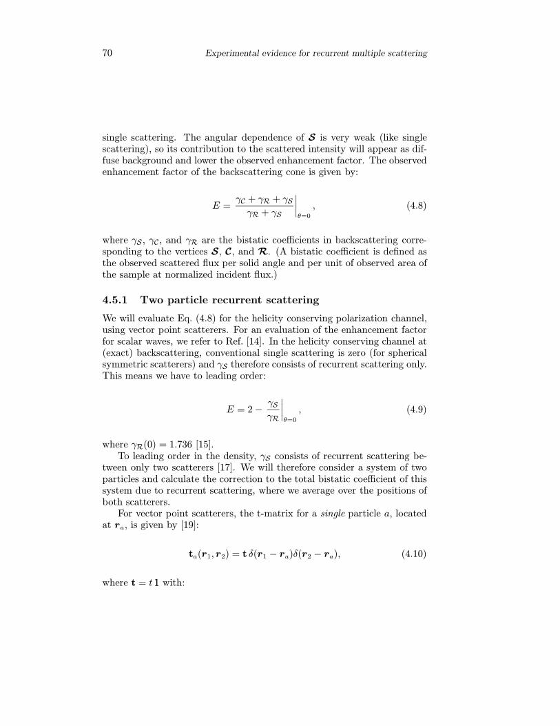
70 Experimental evidence for recurrent multiple scattering
single scattering. The angular dependence of S is very weak (like singlescattering), so its contribution to the scattered intensity will appear as dif-fuse background and lower the observed enhancement factor. The observedenhancement factor of the backscattering cone is given by:
E =γC + γR + γS
γR + γS
∣∣∣∣θ=0
, (4.8)
where γS , γC , and γR are the bistatic coefficients in backscattering corre-sponding to the vertices S, C, and R. (A bistatic coefficient is defined asthe observed scattered flux per solid angle and per unit of observed area ofthe sample at normalized incident flux.)
4.5.1 Two particle recurrent scattering
We will evaluate Eq. (4.8) for the helicity conserving polarization channel,using vector point scatterers. For an evaluation of the enhancement factorfor scalar waves, we refer to Ref. [14]. In the helicity conserving channel at(exact) backscattering, conventional single scattering is zero (for sphericalsymmetric scatterers) and γS therefore consists of recurrent scattering only.This means we have to leading order:
E = 2−γSγR
∣∣∣∣θ=0
, (4.9)
where γR(0) = 1.736 [15].To leading order in the density, γS consists of recurrent scattering be-
tween only two scatterers [17]. We will therefore consider a system of twoparticles and calculate the correction to the total bistatic coefficient of thissystem due to recurrent scattering, where we average over the positions ofboth scatterers.
For vector point scatterers, the t-matrix for a single particle a, locatedat ra, is given by [19]:
ta(r1, r2) = t δ(r1 − ra)δ(r2 − ra), (4.10)
where t = t 11 with:
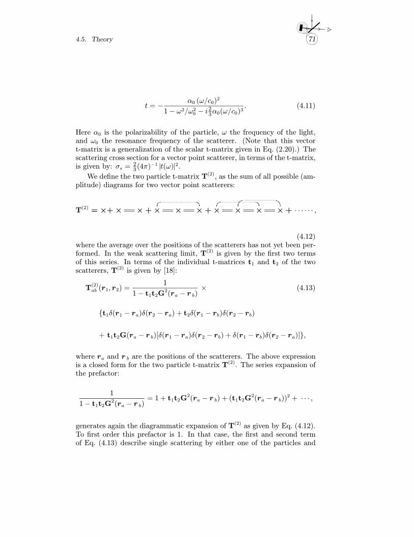
4.5. Theory 71
t = −α0 (ω/c0)
2
1− ω2/ω20 − i23α0(ω/c0)3. (4.11)
Here α0 is the polarizability of the particle, ω the frequency of the light,and ω0 the resonance frequency of the scatterer. (Note that this vectort-matrix is a generalization of the scalar t-matrix given in Eq. (2.20).) Thescattering cross section for a vector point scatterer, in terms of the t-matrix,is given by: σs =
23(4π)
−1 |t(ω)|2.
We define the two particle t-matrix T(2), as the sum of all possible (am-plitude) diagrams for two vector point scatterers:
T(2) = ×+ × × + ×'& %$
× × + ×'& %$
×?> =<
× × + · · · · · · ,
(4.12)where the average over the positions of the scatterers has not yet been per-formed. In the weak scattering limit, T(2) is given by the first two termsof this series. In terms of the individual t-matrices t1 and t2 of the twoscatterers, T(2) is given by [18]:
T(2)ab (r1, r2) =
1
1− t1t2G2(ra − r b)
× (4.13)
{t1δ(r1 − ra)δ(r2 − ra) + t2δ(r1 − rb)δ(r2 − rb)
+ t1t2G(ra − r b)[δ(r1 − ra)δ(r2 − rb) + δ(r1 − rb)δ(r2 − ra)]},
where ra and r b are the positions of the scatterers. The above expressionis a closed form for the two particle t-matrix T(2). The series expansion ofthe prefactor:
1
1− t1t2G2(ra − r b)
= 1 + t1t2G2(ra − r b) + (t1t2G
2(ra − r b))2 + · · · ,
generates again the diagrammatic expansion of T(2) as given by Eq. (4.12).To first order this prefactor is 1. In that case, the first and second termof Eq. (4.13) describe single scattering by either one of the particles and
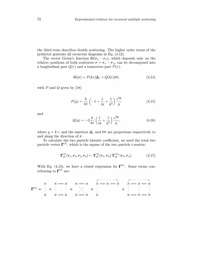
72 Experimental evidence for recurrent multiple scattering
the third term describes double scattering. The higher order terms of theprefactor generate all recurrent diagrams in Eq. (4.12).
The vector Green’s function G(ra − r b), which depends only on therelative positions of both scatterers r = ra − r b, can be decomposed intoa longitudinal part Q(r) and a transverse part P (r):
G(r) = P (kr)∆∆r +Q(kr)rr, (4.14)
with P and Q given by [18]:
P (y) =k
4π
(−1 +
1
iy+
1
y2
)eiy
y(4.15)
and
Q(y) = −2k
4π
(1
iy+
1
y2
)eiy
y, (4.16)
where y = k r, and the matrices ∆∆r and rr are projections respectively toand along the direction of r.
To calculate the two particle bistatic coefficient, we need the total twoparticle vertex ΓΓ(2), which is the square of the two particle t-matrix:
ΓΓ(2)ab (r1, r2, r3, r4) = T
(2)ab (r1, r2) T
(2)∗ab (r3, r4). (4.17)
With Eq. (4.13), we have a closed expression for ΓΓ(2). Some terms con-
tributing to ΓΓ(2) are:
ΓΓ(2) =
×
×
+
× ×
× ×
+
× ×
× ×
+
×'& %$
× ×
×
+
×'& %$
× ×
× × ×
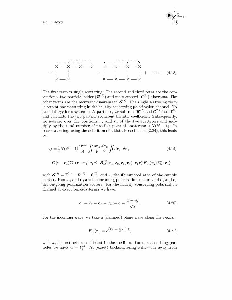
4.5. Theory 73
+
×'& %$
×?> =<
× ×
× ×
+
×'& %$
×?> =<
× ×
× × × ×
+ · · · · · · (4.18)
The first term is single scattering. The second and third term are the con-ventional two particle ladder (R(2)) and most-crossed (C(2)) diagrams. The
other terms are the recurrent diagrams in S(2). The single scattering termis zero at backscattering in the helicity conserving polarization channel. Tocalculate γS for a system of N particles, we subtractR(2) and C(2) from ΓΓ(2)
and calculate the two particle recurrent bistatic coefficient. Subsequently,we average over the positions ra and r b of the two scatterers and mul-tiply by the total number of possible pairs of scatterers: 12N(N − 1). Inbackscattering, using the definition of a bistatic coefficient (2.34), this leadsto:
γS = 12N(N − 1)
4πr2
A
∫∫draV
dr bV
∫∫dr1..dr4 (4.19)
G(r −r1)G∗(r −r3)e1e
∗3 ·S
(2)ab (r1, r2, r3, r4) ·e2e
∗4 Ein(r2)E
∗in(r4),
with S(2) = ΓΓ(2) −R(2) − C(2), and A the illuminated area of the samplesurface. Here e2 and e4 are the incoming polarization vectors and e1 and e3the outgoing polarization vectors. For the helicity conserving polarizationchannel at exact backscattering we have:
e1 = e2 = e3 = e4 := e =x+ iy√2
. (4.20)
For the incoming wave, we take a (damped) plane wave along the z-axis:
Ein(r ) = e(ik −12κe) z, (4.21)
with κe the extinction coefficient in the medium. For non absorbing par-ticles we have κe = −1s . At (exact) backscattering with r far away from
74 Experimental evidence for recurrent multiple scattering
the medium, the longitudinal component of G(r −r1) can be neglected soG(r −r1) is given by:
G(r −r1) = G(r −r1) ∆∆r (4.22)
where G(r −r1) can be approximated by (see Eq. (2.36)):
G(r −r1) −eikr
4πre−ikz ·r1 −
12κez1 . (4.23)
Because S is short range we can put r1 r2 r3 r4. After performingthe integration over r1..r4 we find:
γS =N2
2V 21
4πA
∫drae−2κeza
∫d(ra− r b) ee
∗·S(2)(ra− r b) ·ee∗ , (4.24)
where we have used that 12N(N − 1) 12N
2 because N is very large. Afterperforming the integral over ra and taking the limit N →∞, V →∞, withN/V → n, we find the bistatic coefficient describing two particle recurrentscattering:
γS =3n
8 |t |2
∫dr ee∗·S(2)(r) · ee∗ , (4.25)
where we have used that s = 1/(nσs) = 6π/(n|t|2). If we divide the aboveexpression by γR, we find the first order density correction to the enhance-ment factor in going to strong scattering, and [according to Eq. (4.9)] theenhancement factor itself becomes:
E = 2− n3
γR(0) 8|t |2
∫dr ee∗ · S(2)(r) · ee∗. (4.26)
The integral over the separation vector r can be performed numerically.Furthermore, because our samples are strongly polydisperse, we averaget1 and t2 independently over a frequency window which is large comparedto the width of the resonance. The enhancement factor calculated withEq. (4.26), is plotted in Fig. 4.5 as a dashed line. We see that the calculationconfirms our interpretation that recurrent scattering manifests itself as areduction of the enhancement factor for k s <∼ 10.
75
References and notes
[1] P.W. Anderson, Phys. Rev. 109, 1492 (1958); Anderson Localization,edited by T. Ando and H. Fukuyama, in Springer proceedings in physics28 (Springer, Berlin, 1988).
[2] Analogies in Optics and Micro Electronics, edited by W. van Haeringenand D. Lenstra (Kluwer, Dordrecht, 1990).
[3] D. Vollhardt and P. Wolfle, in Electronic Phase Transitions, ModernProblems in Condensed Matter Sciences 32, edited by W. Hanke andYu. V. Kopaev (North-Holland, Amsterdam, 1992).
[4] B.L. Altshuler, A.G. Aronov, D.E. Khmel’nitskii, and A.I. Larkin, inQuantum Theory of Solids, edited by I.M. Lifshitz (MIR Publishers,Moskva, 1983).
[5] A.F. Ioffe and A.R. Regel, Progr. Semiconductors 4, 237 (1960); N.F.Mott, Metal-Insulator Transitions (Taylor and Francis, London, 1974).
[6] The TiO2 powders were obtained from Sachtleben Chemie, Duisburg,and are of the type RCL 6G rutil TiO2.
[7] SpectraflectTM is a trademark of Labsphere, Inc. North Sutton, UnitedStates.
[8] W is the full width at half maximum. IfW is varied, the backscatteringcone scales linearly along the x-axis.
[9] M.B. van der Mark, M.P. van Albada, and A. Lagendijk, Phys. Rev. B37, 3575 (1988); P.E. Wolf, G. Maret, E. Akkermans, and R. Maynard,J. Phys. France 49, 63 (1988); further developed to handle semi-infiniteslabs in: E.E. Gorodnichev, S.L. Dudarev, and D.B. Rogozkin, Phys.Lett. A 144, 48 (1990).
[10] A. Lagendijk, B. Vreeker, and P. de Vries, Phys. Lett. A 136, 81 (1989);J.X. Zhu, D.J. Pine, and D.A. Weitz, Phys. Rev. A 44, 3948 (1991).
[11] In order to be able to compare the data with the calculation on twoparticle recurrent scattering (presented in section 4.5), we have to as-sume that = s. The mean free path induced from the cone width isthe transport mean free path and not the scattering mean free path.If the particles scatter anisotropically, will be larger than s. In thelast section, we will see that despite this assumption, the agreementbetween data and theory is good.
[12] P.N. den Outer and A. Lagendijk, Opt. Comm. 103, 169 (1993).[13] D. Vollhardt and P. Wolfle, Phys. Rev. B 22, 4666 (1980).[14] B.A. van Tiggelen, D.S. Wiersma, and A. Lagendijk, Europhys. Lett.
30, 1 (1995).[15] The value was derived using γ++r0 +γ+−r0 +γ+−s0 = 4×1.1471 by Table 54
of Ref. [16], treating single and double scattering exactly and the rest
76
in the diffusion approximation (see E. Akkermans and R. Maynard, J.Phys. (Paris) Lett. 46, 1045 (1985); M.P. van Albada and A. Lagendijk,Phys. Rev. B 36, 2353 (1987)).
[16] H.C. van de Hulst, Multiple Light Scattering (Dover, New York, 1980).[17] B.A. van Tiggelen and A. Lagendijk, Phys. Rev. B 22, 16729 (1994).[18] B.A. van Tiggelen, A. Lagendijk, and A. Tip, J. Phys. C 2, 7653 (1990).[19] H.J. Dorren and A. Tip, J. Math. Phys. 32, 3060 (1991); Th.M.
Nieuwenhuizen, A. Lagendijk, and B.A. van Tiggelen, Phys. Lett. A169, 191 (1993).
Chapter 5
Amplifying random media
5.1 Introduction
This chapter is concerned with the experimental considerations on creatingdisordered media that exhibit optical amplification. We will show howto create a medium in which light waves are both multiply scattered andamplified in between or during the scattering events. Optical amplificationis obtained through stimulated emission in a laser material. To introducescattering in such a material, one can grind a laser crystal like ruby orTi:sapphire. Another option is to use latex microparticle combined withlaser dye, either by suspending the particles in a dye solution or by dopingthe particles with the dye.
To obtain amplification, the laser material must be brought in inversion.This excitation is called pumping and can for instance be done opticallywith intense laser light. One encounters several problems however, that donot occur in conventional laser systems. In a conventional laser system, thepump light is absorbed by the laser material, which is thereby brought intothe desired excited state. If scattering is introduced in such a laser material,the pump light will be both scattered and absorbed. If the scattering ismuch stronger than the absorption, most of the pump light is scatteredout of the system without being absorbed. We will look into this problemand discuss pumping geometries that can be used to increase the pumpingefficiency.
The intensities required to excite a laser material are high, which isa complicating factor in the experiments. With a continuous wave (CW)laser, they can be obtained only if the light is focused to a diameter of afew tens of micro meters, and the resulting excited volume will thereforebe very small. If we wish to excite a larger volume, we are forced to use
77
78 Amplifying random media
pulsed pump light. This means that our disordered laser material will notamplify continuously, but only during some limited time window (rangingfrom 10 ns to several ms), at a certain repetition rate.
In this chapter we will go into the various possibilities of creating am-plifying random media, and show some results on powdered laser crystals.
5.1.1 Relevant length scales
In an amplifying random medium, light waves are both multiply scatteredand amplified. The relevant length scales that describe the scattering pro-cess are the scattering mean free path s and transport mean free path , asthey were defined in chapter 2. To describe the amplification process, wedefine two new length scales: the gain length g and amplification length amp. The gain length is defined as the path length over which the intensityis amplified by a factor e+1. The amplification length is defined as the (rms)average distance between the begin and end points for paths of length g:
amp ≡
√ g3
. (5.1)
Without scattering, amp is equal to g. The amplification length ampand gain length g are the analogues of the absorption length abs and theinelastic length i that describe absorption.
For an amplifying medium one can define a critical volume above whichthe system becomes unstable. The average total amplification for a waveinside the sample increases with the volume of the sample, whereas theloss through the boundaries is proportional to the boundary surface. Thecritical volume Vcr is defined as the volume at which gain equals loss. Abovethe critical volume, the intensity inside the medium diverges.
We will study samples with a slab geometry. In that case, one candefine a critical thickness Lcr instead of a critical volume, above which theintensity diverges. The critical thickness is given by (see section 6.3.5):
Lcr = π amp = π
√ g3
. (5.2)
Note that Lcr is proportional to amp.
5.2. Realizing disordered media with gain 79
5.2 Realizing disordered media with gain
5.2.1 Choice of the laser material
An important factor in realizing an amplifying randommedium is the choiceof the laser material. We will consider laser materials which are opticallypumped. Most laser material can be described as a three or four levelsystem. The material is excited optically to some high energy level thatdecays rapidly to a metastable state. The laser transition occurs from thismetastable state to the ground state or to a short lived (and thereby nearlyunpopulated) state above the ground state. (See also section 1.2.)
The relevant cross sections are the absorption cross section σPabs of thepump transition and the stimulated emission cross section σLem of the lasertransition. The emission cross section σLem, determines the maximum gainof the system and should therefore be as large as possible. Amplificationis achieved only when the gain at the emission wavelength is larger thanthe absorption at this wavelength. The advantage of a four level system isthat the ground state of the laser transition is almost unpopulated, so theabsorption at the emission wavelength in principle can be very small. Foran amplifying random medium, it is more important that σPabs is large thanit is for regular laser systems. The absorption cross section determinesthe inelastic length i for the pump light. If i is much larger than thetransport mean free path , most pump light is scattered without beingabsorbed. We come back to this problem in the next section. In Table 5.1,we have listed σPabs and σLem for some laser materials. Also listed is the ratioof the absorption coefficient to the maximum gain coefficient at the peakemission wavelength.
Another important parameter is the excited state lifetime τe. Becausewe have to use pulsed pump light, the lifetime of the overall gain in thesystem will be limited by τe. If the excited part of the medium is muchsmaller than the critical volume Vcr, it will be equal to τe. Close to thecritical volume, the lifetime of the overall gain is much shorter than τe,because spontaneously emitted light will be largely amplified, thereby de-exciting the system. We come back to these effects in section 5.3.
From Table 5.1, we see that the lifetime of the excited state for ruby isvery large. Unfortunately, this material is a three level system and there-fore the absorption at the emission wavelength is large (κabs/κg = 0.5).Laser dye like Rhodamine 6G has the advantage of a very large absorptionand emission cross section. However, experiments with dye have to be per-formed with picosecond time resolution due to the very short lifetime of theexcited state. Nd:YAG has a reasonably large emission cross section and
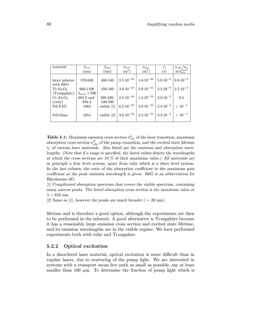
80 Amplifying random media
material λem λabs σem σabs τe κabs/κg(nm) (nm) (m2) (m2) (s) atλmaxem
latex spheres 570-630 460-540 2.5·10−20 1.6·10−20 5.0·10−9 6.8·10−6
with R6GTi:Al2O3 660-1100 450-580 3.0·10−23 3.0·10−24 3.2·10−6 2.5·10−3
(Ti:sapphire) λmax �780Cr:Al2O3 692.9 and 380-430; 2.5·10−24 1.2·10−24 3.0·10−3 0.5(ruby) 694.3 520-590Nd:YAG 1064 visible [1] 6.5·10−23 3.6·10−24 2.3·10−4 < 10−4
Nd:Glass 1054 visible [2] 3.0·10−24 2.3·10−24 3.3·10−4 < 10−4
Table 5.1: Maximum emission cross section σLem of the laser transition, maximum
absorption cross section σPabs of the pump transition, and the excited state lifetime
τe of various laser materials. Also listed are the emission and absorption wave-
lengths. (Note that if a range is specified, the listed values denote the wavelengths
at which the cross sections are 10 % of their maximum value.) All materials are
in principle a four level system, apart from ruby which is a three level system.
In the last column, the ratio of the absorption coefficient to the maximum gain
coefficient at the peak emission wavelength is given. R6G is an abbreviation for
Rhodamine 6G.
[1] Complicated absorption spectrum that covers the visible spectrum, containing
many narrow peaks. The listed absorption cross section is the maximum value at
λ = 810 nm.
[2] Same as [1], however the peaks are much broader ( ∼ 20 nm).
lifetime and is therefore a good option, although the experiments are thento be performed in the infrared. A good alternative is Ti:sapphire becauseit has a reasonably large emission cross section and excited state lifetime,and its emission wavelengths are in the visible regime. We have performedexperiments both with ruby and Ti:sapphire.
5.2.2 Optical excitation
In a disordered laser material, optical excitation is more difficult than inregular lasers, due to scattering of the pump light. We are interested insystems with a transport mean free path as small as possible, say at leastsmaller than 100 µm. To determine the fraction of pump light which is
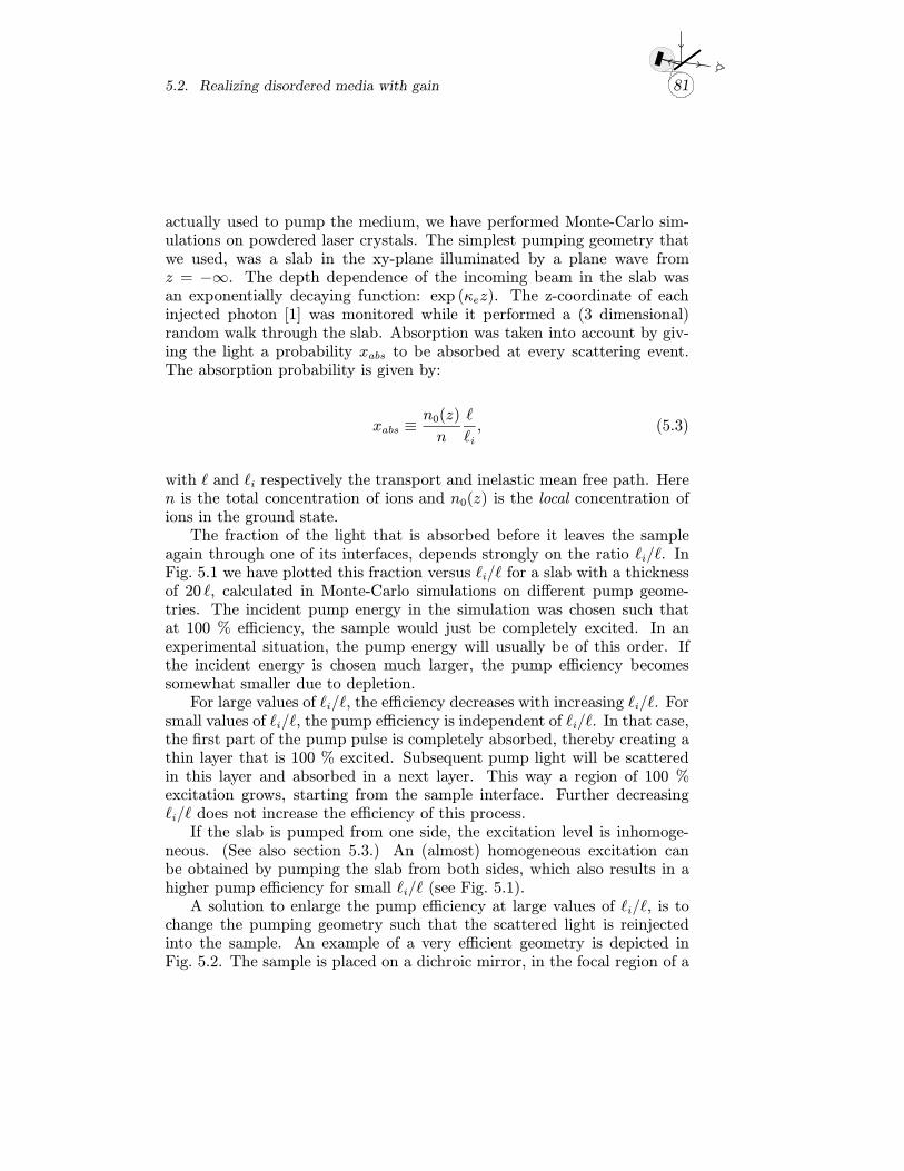
5.2. Realizing disordered media with gain 81
actually used to pump the medium, we have performed Monte-Carlo sim-ulations on powdered laser crystals. The simplest pumping geometry thatwe used, was a slab in the xy-plane illuminated by a plane wave fromz = −∞. The depth dependence of the incoming beam in the slab wasan exponentially decaying function: exp (κez). The z-coordinate of eachinjected photon [1] was monitored while it performed a (3 dimensional)random walk through the slab. Absorption was taken into account by giv-ing the light a probability xabs to be absorbed at every scattering event.The absorption probability is given by:
xabs ≡n0(z)
n
i, (5.3)
with and i respectively the transport and inelastic mean free path. Heren is the total concentration of ions and n0(z) is the local concentration ofions in the ground state.
The fraction of the light that is absorbed before it leaves the sampleagain through one of its interfaces, depends strongly on the ratio i/ . InFig. 5.1 we have plotted this fraction versus i/ for a slab with a thicknessof 20 , calculated in Monte-Carlo simulations on different pump geome-tries. The incident pump energy in the simulation was chosen such thatat 100 % efficiency, the sample would just be completely excited. In anexperimental situation, the pump energy will usually be of this order. Ifthe incident energy is chosen much larger, the pump efficiency becomessomewhat smaller due to depletion.
For large values of i/ , the efficiency decreases with increasing i/ . Forsmall values of i/ , the pump efficiency is independent of i/ . In that case,the first part of the pump pulse is completely absorbed, thereby creating athin layer that is 100 % excited. Subsequent pump light will be scatteredin this layer and absorbed in a next layer. This way a region of 100 %excitation grows, starting from the sample interface. Further decreasing i/ does not increase the efficiency of this process.
If the slab is pumped from one side, the excitation level is inhomoge-neous. (See also section 5.3.) An (almost) homogeneous excitation canbe obtained by pumping the slab from both sides, which also results in ahigher pump efficiency for small i/ (see Fig. 5.1).
A solution to enlarge the pump efficiency at large values of i/ , is tochange the pumping geometry such that the scattered light is reinjectedinto the sample. An example of a very efficient geometry is depicted inFig. 5.2. The sample is placed on a dichroic mirror, in the focal region of a
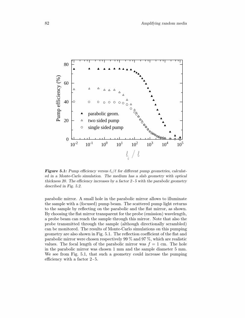
82 Amplifying random media
10-2 10-1 100 101 102 103 104 1050
20
40
60
80
parabolic geom. two sided pumpsingle sided pump
Pum
p ef
fici
ency
(%
)
Figure 5.1: Pump efficiency versus i/ for different pump geometries, calculat-
ed in a Monte-Carlo simulation. The medium has a slab geometry with optical
thickness 20. The efficiency increases by a factor 2 - 5 with the parabolic geometry
described in Fig. 5.2.
parabolic mirror. A small hole in the parabolic mirror allows to illuminatethe sample with a (focused) pump beam. The scattered pump light returnsto the sample by reflecting on the parabolic and the flat mirror, as shown.By choosing the flat mirror transparent for the probe (emission) wavelength,a probe beam can reach the sample through this mirror. Note that also theprobe transmitted through the sample (although directionally scrambled)can be monitored. The results of Monte-Carlo simulations on this pumpinggeometry are also shown in Fig. 5.1. The reflection coefficient of the flat andparabolic mirror were chosen respectively 99 % and 97 %, which are realisticvalues. The focal length of the parabolic mirror was f = 1 cm. The holein the parabolic mirror was chosen 1 mm and the sample diameter 5 mm.We see from Fig. 5.1, that such a geometry could increase the pumpingefficiency with a factor 2 - 5.
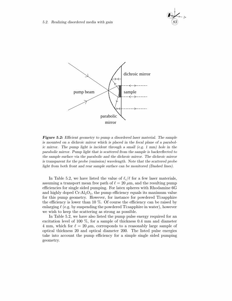
5.2. Realizing disordered media with gain 83
sample
dichroic mirror
parabolic
mirror
pump beam
Figure 5.2: Efficient geometry to pump a disordered laser material. The sample
is mounted on a dichroic mirror which is placed in the focal plane of a parabol-
ic mirror. The pump light is incident through a small (e.g. 1 mm) hole in the
parabolic mirror. Pump light that is scattered from the sample is backreflected to
the sample surface via the parabolic and the dichroic mirror. The dichroic mirror
is transparent for the probe (emission) wavelength. Note that the scattered probe
light from both front and rear sample surface can be monitored (Dashed lines).
In Table 5.2, we have listed the value of i/ for a few laser materials,assuming a transport mean free path of = 20 µm, and the resulting pumpefficiencies for single sided pumping. For latex spheres with Rhodamine 6Gand highly doped Cr:Al2O3, the pump efficiency equals its maximum valuefor this pump geometry. However, for instance for powdered Ti:sapphirethe efficiency is lower than 10 %. Of course the efficiency can be raised byenlarging (e.g. by suspending the powdered Ti:sapphire in water), howeverwe wish to keep the scattering as strong as possible.
In Table 5.2, we have also listed the pump pulse energy required for anexcitation level of 100 %, for a sample of thickness 0.4 mm and diameter4 mm, which for = 20 µm, corresponds to a reasonably large sample ofoptical thickness 20 and optical diameter 200. The listed pulse energiestake into account the pump efficiency for a simple single sided pumpinggeometry.
84 Amplifying random media
material ion/mol. i i/ pump pulseconc. eff. energy
(1025 m−3) (m) (mJ)latex spheres 1.3 5.0·10−5 2.5 40 % 6.0with R6GTi:Al2O3 (0.15%) 4.7 2.3·10−2 1.17·103 7.7 % 351Cr:Al2O3 (0.05%) 1.6 2.5·10−2 1.23·103 7.4 % 122Cr:Al2O3 (2.1%) 67 5.9·10−4 2.92·101 38 % 992Nd:YAG (1.1%) 14 2.0·10−3 1.0·102 29 % 269Nd:Glass (5.0%) 48 0.9·10−3 4.5·101 35 % 771
Table 5.2: Pump efficiency for some laser materials assuming a transport mean
free path = 20 µm. The inelastic mean free path i was calculated from the
maximum absorption cross section assuming a volume fraction of 30 % powdered
laser crystal or 10 % latex spheres with R6G. Also listed is the required pump
energy to fully excite a slab of thickness 0.4 mm and diameter 4.0 mm, taking into
account the pump efficiency. The higher internal energy density in the scatterers
compared to their environment [2,3], is not taken into account. This would yield
smaller values of i (by a factor of 2 - 4) which would result in more efficient
pumping.
5.2.3 Experimentally realized gain levels
We have performed experiments on ruby and Ti:sapphire because of theirreasonably large emission cross section and excited state lifetime. To obtainthe required pulse energy to excite these materials, we have used a frequen-cy doubled Q-switched Nd:YAG laser with a pulse duration of 14 ns. Themaximum pulse energy incident on the sample was about 200 mJ, whichfor a beam diameter of 5 mm corresponds to a maximum incident intensityof 7.3·1011 J/m2s. A low intensity probe pulse was incident at a time delayof 14 ns after the pump pulse, on the same side of the sample. (Probe pulseenergy 40 µJ, pulse duration 14 ns, and beam diameter 5 mm. Probe andpump beam overlap on the sample surface.) The temporal profile of thetransmitted and backscattered intensity was recorded. The overall amplifi-cation in transmission and in backscattering was determined by comparingthe probe intensity with and without pump light. To avoid artifacts fromcumulative heating of the sample after many pump pulses or other longterm effects, the repetition rate of the probe was chosen twice as high at
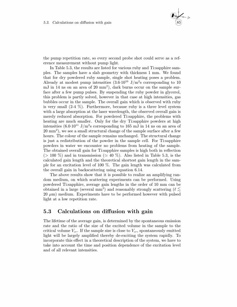
5.3. Calculations on diffusion with gain 85
the pump repetition rate, so every second probe shot could serve as a ref-erence measurement without pump light.
In Table 5.3, the results are listed for various ruby and Ti:sapphire sam-ples. The samples have a slab geometry with thickness 1 mm. We foundthat for dry powdered ruby sample, single shot heating poses a problem.Already at modest pump intensities (3.6·1010 J/m2s corresponding to 10mJ in 14 ns on an area of 20 mm2), dark burns occur on the sample sur-face after a few pump pulses. By suspending the ruby powder in glycerol,this problem is partly solved, however in that case at high intensities, gasbubbles occur in the sample. The overall gain which is observed with rubyis very small (2-4 %). Furthermore, because ruby is a three level systemwith a large absorption at the laser wavelength, the observed overall gain ismerely reduced absorption. For powdered Ti:sapphire, the problems withheating are much smaller. Only for the dry Ti:sapphire powders at highintensities (6.0·1011 J/m2s corresponding to 165 mJ in 14 ns on an area of20 mm2), we see a small structural change of the sample surface after a fewhours. The colour of the sample remains unchanged. The structural changeis just a redistribution of the powder in the sample cell. For Ti:sapphirepowders in water we encounter no problems from heating of the sample.The obtained overall gain for Ti:sapphire samples is high both in reflection(> 100 %) and in transmission ( 40 %). Also listed in Table 5.3, is thecalculated gain length and the theoretical shortest gain length in the sam-ple for an excitation level of 100 %. The gain length was calculated fromthe overall gain in backscattering using equation 6.14.
The above results show that it is possible to realize an amplifying ran-dom medium, on which scattering experiments can be performed. Usingpowdered Ti:sapphire, average gain lengths in the order of 10 mm can beobtained in a large (several mm3) and reasonably strongly scattering ( <∼20 µm) medium. Experiments have to be performed however with pulsedlight at a low repetition rate.
5.3 Calculations on diffusion with gain
The lifetime of the average gain, is determined by the spontaneous emissionrate and the ratio of the size of the excited volume in the sample to thecritical volume Vcr. If the sample size is close to Vcr, spontaneously emittedlight will be largely amplified thereby de-exciting the system rapidly. Toincorporate this effect in a theoretical description of the system, we have totake into account the time and position dependence of the excitation leveland of all relevant intensities.
86 Amplifying random media
transmission datamaterial in L pump int. overall remarks
µm µm J/m2s gainruby air 200 10 3.6·1010 - dark burnsruby glycerol 100 40 3.6·1011 2-4 %ruby glycerol 100 40 7.3·1011 - gas bubblesTi:sapphire air 100 10 1.6·1011 16-18 %Ti:sapphire air 100 10 2.5·1011 25-31 %Ti:sapphire air 100 10 3.6·1011 30 %Ti:sapphire air 175 10 2.1·1011 38 %Ti:sapphire air 175 10 3.0·1011 42 %Ti:sapphire air 100 10 6.0·1011 - struc. change
backscattering datamaterial in L pump int. overall g ming
µm µm J/m2s gain mm mmTi:sapphire water 1000 40 6.0·1011 36 % 13.9 2.3Ti:sapphire water 1000 40 6.9·1011 71 % 11.2 2.3Ti:sapphire water 1000 28 6.5·1011 115 % 13.4 2.3Ti:sapphire air [1] 1000 18 6.5·1011 155 % 18.6 2.3Ti:sapphire air [1] 1000 18 6.9·1011 134 % 18.5 2.3
Table 5.3: Results of transmission and backscattering measurements on the over-
all gain from powdered ruby (2.1 wt% Cr2O3) and powdered Ti:sapphire (0.15 wt%
Ti2O3). Pump wavelength 532 nm, pulse duration 14 ns. The ruby/air samples
get burnt already at modest pump intensities. The ruby/glycerol samples show
air bubbles at high intensities. The gain of 2-4 % observed for ruby is in reality re-
duced absorption. With the Ti:sapphire, a large gain is obtained without damage
to the sample. Only at the highest pump intensities, a slight structural change is
visible for the Ti:sapphire/air sample.
[1] The medium consists of wet Ti:sapphire particles surrounded by air, and is
therefore somewhat larger than for a completely dry Ti:sapphire powder.
5.3. Calculations on diffusion with gain 87
If we assume the propagation of light in the sample to be diffusive,we can describe the time and position-dependent energy density of boththe pump and probe light by a diffusion equation with an absorption re-spectively gain term that depends on the local excitation of the sample.The time and position-dependent excitation level is described by the rateequations of the laser material. Apart from the probe and pump light,we have to account for amplified spontaneous emission (ASE). We denotethe energy density of the (green) pump light by WG(r, t), the (red) probelight by WR(r, t), and the amplified spontaneous emission by WA(r, t). Foreach position and time-dependent energy density, we can write a diffusionequation with the appropriate source terms. Absorption of ASE or probelight is not taken into account. The concentration N1(r, t) of excited laserparticles (ions, molecules, . . . ) is determined by the rate equation of thelaser material. We assume a four level laser system as described in theprevious section, with a very fast decay rate from level (2) to level (1) andfrom level (0’) to the ground state (0), which means level (2) and level (0’)are nearly unpopulated. The excitation level is given by N1(r, t)/Nt, withNt the total concentration of laser particles. We arrive at the following setof coupled differential equations describing our system:
∂WG(r, t)
∂t= D∇2WG(r, t)− σabsv[Nt−N1(r, t)]WG(r, t)+
1
IG(r, t) (5.4)
∂WR(r, t)
∂t= D∇2WR(r, t) + σemvN1(r, t)WR(r, t) +
1
IR(r, t) (5.5)
∂WA(r, t)
∂t= D∇2WA(r, t) + σemvN1(r, t)WA(r, t) +
n
τeN1(r, t) (5.6)
∂N1(r, t)
∂t= σabsv[Nt −N1(r, t)]WG(r, t)
−σemvN1(r, t)[WR(r, t) +WA(r, t)]−1
τeN1(r, t),
where v is the transport velocity of the light inside the medium, σabs andσem are respectively the absorption and emission cross section, and τe isthe lifetime of the excited state. D is the diffusion constant given by:
D =v
3, (5.7)
and IG(r, t) and IR(r, t) are the intensities of respectively the incomingpump and probe pulses. For simplicity, we use the same value of the diffu-
88 Amplifying random media
sion constant for the pump and probe light, and for the ASE. The probepulse is incident on the front sample interface. The pump pulse is eitherincident on both the front and rear interface or on the front interface only.In the latter case we have:
IG(r, t) = IG0
√b
πexp [−κez] exp [−b
(t− tG − z/c)2
τ 2G], (5.8)
and
IR(r, t) = IR0
√b
πexp [−κez] exp [−
(t− tR − z/c)2
τ 2R], (5.9)
where b = 4 ln(2), κe −1 is the extinction coefficient, and c = c0/n, withn the effective refractive index of the medium.
Here IG0 and IR0 are the average intensities of respectively the pumpand probe light, τG and τR are the pulse lengths (FWHM) of respectivelythe pump and probe pulse, and tG and tR are the points in time at whichthe maximum of respectively the pump and probe pulse is incident on thesample surface. If the pump pulse is incident on both sample interfaces wemodify Eq. (5.8) to:
IG(r, t) = IG0
√b
π
exp [−κez] + exp [−κe(L− z)]
2exp [−b
(t− tG − z/c)2
τ 2G].
(5.10)
We consider a slab with thickness L, which leads to the spatial boundarycondition:
WG(r, t) = WR(r, t) = WA(r, t) = 0, (5.11)
forz = −z0 and z = L+ z0. (5.12)
where z0 0.71 is the extrapolation length, as defined in section 2.2. Thepoints in time tG and tR at which pump and probe pulse are incident aretaken positive and large compared to the pulse lengths τG and τR. Thereforeall energy densities are zero before t = 0:
WG(r, t ≤ 0) = WR(r, t ≤ 0) = WA(r, t ≤ 0) = 0. (5.13)
5.3. Calculations on diffusion with gain 89
5.3.1 Discretization
Because our system is a slab in the xy-plane illuminated by plane waves inthe z-direction, we can omit the x and y dependence of the energy densities.This means we can retain only the partial derivative to z in the gradientsin Eqns. (5.4) to (5.7).
The resulting set of coupled partial differential equations can be solvednumerically using a standard (forward Euler) discretization for the timederivative:
∂f(z, t)
∂t:=
f(z, t+∆t)− f(z, t)
∆t(5.14)
and for the second order space derivative the straightforward discretization:
∂2f(z, t)
∂z2:=
f(z +∆z, t)− 2f(z, t) + f(z −∆z, t)
∆z2. (5.15)
This discretization method has the advantage that it is simple and explicit,that is, the discretization of the space derivative depends only on f(z, t)and not on f(z, t + ∆t). The disadvantage is that for small ∆z, the timesteps ∆t have to be taken very small, to satisfy the stability criterion [4]:
∆t ≤∆z2
2D. (5.16)
The physical interpretation of this criterion is that, apart from a numericalfactor, the time steps have to be smaller than the diffusion time across adistance ∆z. The descretized set of equations is:
WG(z, t+∆t)−WG(z, t) = ∆t{DWG(z+∆z, t)+WG(z−∆z, t)−2WG(z, t)
∆z2
−σabsv[Nt −N1(z, t)]WG(z, t) + −1IG(z, t)} (5.17)
WR(z, t+∆t)−WR(z, t) = ∆t{DWR(z+∆z, t)+WR(z−∆z, t)−2WR(z, t)
∆z2
+σemvN1(z, t)WR(z, t) + −1IR(z, t)} (5.18)
WA(z +∆z, t)−WA(z, t) = ∆t{DWA(z+∆z, t)+WA(z−∆z, t)−2WA(z, t)
∆z2
90 Amplifying random media
+σemvN1(z, t)WA(z, t) +1
τeN1(z, t)} (5.19)
N1(z +∆z, t)−N1(z, t) = ∆t{σabsv[Nt −N1(z, t)]WG(z, t) (5.20)
−σemvN1(z, t)[WR(z, t) +WA(z, t)] −1
τeN1(z, t)},
5.3.2 Backscattered flux
Solving the above set of partial differential equations numerically for prac-tical values of σabs, σem, and τe at different pump intensities and values of , provides us with information about the spatial and temporal distributionof all relevant energy densities and the excitation level inside the sample.Also we can calculate the outgoing flux at either the front or rear interfaceof the slab, which is determined by the gradient of the energy density at thesample interface. For the outgoing probe flux at the front sample interface,we have:
W outR (t) ≡ AsD
∂WR(0, t)
∂z= AsD
WR(0, t)
z0, (5.21)
where As is the area of the sample surface. Here we have used thatWR(z, t)is zero for z = −z0.
In Fig 5.3 we have plotted the outgoing probe flux for a powderedTi:sapphire sample (doping level 0.15 wt% Ti2O3) of 0.8 mm thicknessand 4 mm diameter, with a transport mean free path = 40 µm, for twopumping geometries. In the upper graph, the sample is pumped from oneside with 14 ns pulses at 532 nm, with pulse energy 200 mJ. In the lowergraph, the same total pump energy is incident on the sample, but nowequally distributed over front and rear sample interface. The dotted linesindicate the incoming pump and probe pulses, and the dashed line denotesthe outgoing probe flux without amplification. The latter is slightly lowerthan the incoming probe flux due to the finite sample thickness which allowssome probe flux to disappear through the back sample interface. The ratioof the amplified to the unamplified outgoing probe flux indicates the averageoverall gain in the sample. Here the overall gain is 163% for single sidedand 142% for double sided pumping.
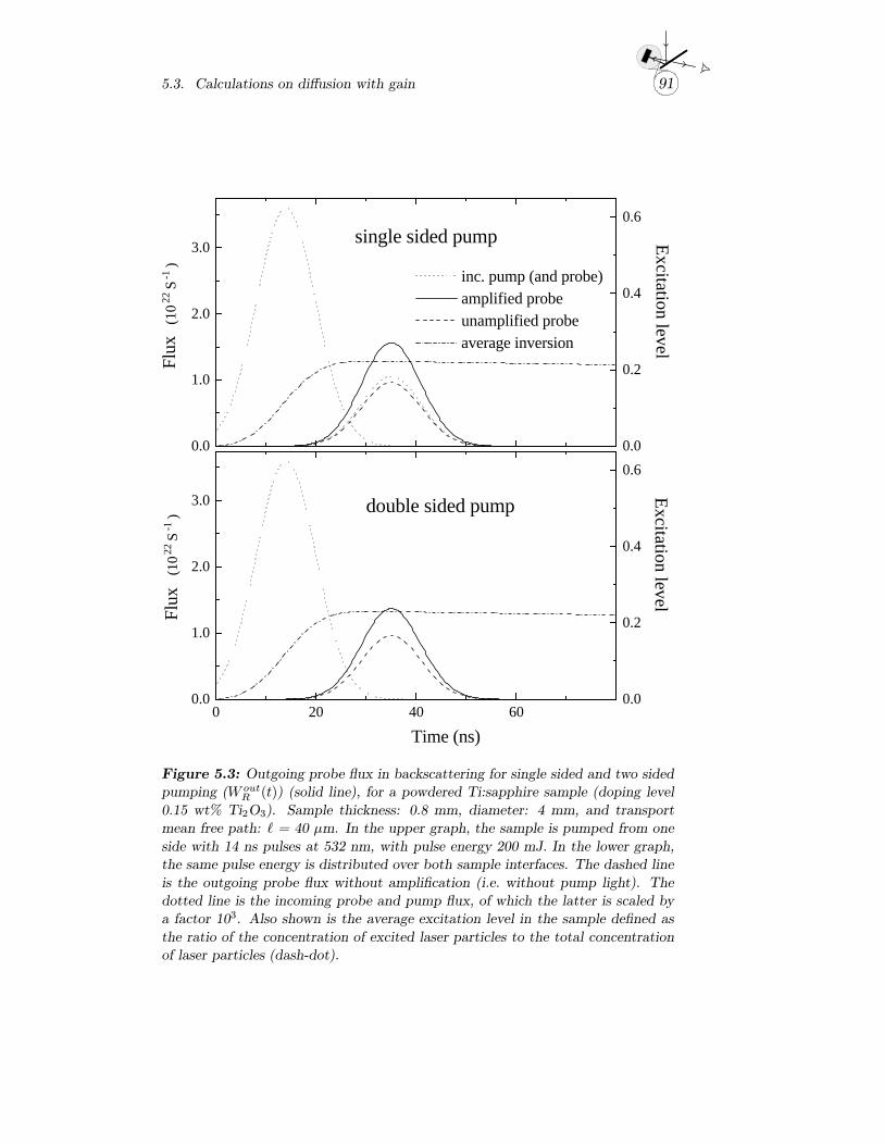
5.3. Calculations on diffusion with gain 91
0 20 40 600.0
1.0
2.0
3.0
(10 2
2 S -
1 )(1
0 22 S
-1 )
Flux
Time (ns)
0.0
0.2
0.4
0.6
double sided pump
Excitation level
0.0
1.0
2.0
3.0
Flux
inc. pump (and probe) amplified probe unamplified probe average inversion
single sided pump
0.0
0.2
0.4
0.6E
xcitation level
Figure 5.3: Outgoing probe flux in backscattering for single sided and two sided
pumping (W outR (t)) (solid line), for a powdered Ti:sapphire sample (doping level
0.15 wt% Ti2O3). Sample thickness: 0.8 mm, diameter: 4 mm, and transport
mean free path: = 40 µm. In the upper graph, the sample is pumped from one
side with 14 ns pulses at 532 nm, with pulse energy 200 mJ. In the lower graph,
the same pulse energy is distributed over both sample interfaces. The dashed line
is the outgoing probe flux without amplification (i.e. without pump light). The
dotted line is the incoming probe and pump flux, of which the latter is scaled by
a factor 103. Also shown is the average excitation level in the sample defined as
the ratio of the concentration of excited laser particles to the total concentration
of laser particles (dash-dot).
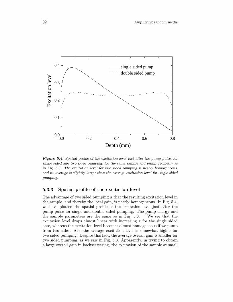
92 Amplifying random media
0.0 0.2 0.4 0.6 0.80.0
0.1
0.2
0.3
0.4 single sided pump
double sided pump
Exc
itat
ion
leve
l
Depth (mm)
Figure 5.4: Spatial profile of the excitation level just after the pump pulse, for
single sided and two sided pumping, for the same sample and pump geometry as
in Fig. 5.3. The excitation level for two sided pumping is nearly homogeneous,
and its average is slightly larger than the average excitation level for single sided
pumping.
5.3.3 Spatial profile of the excitation level
The advantage of two sided pumping is that the resulting excitation level inthe sample, and thereby the local gain, is nearly homogeneous. In Fig. 5.4,we have plotted the spatial profile of the excitation level just after thepump pulse for single and double sided pumping. The pump energy andthe sample parameters are the same as in Fig. 5.3. We see that theexcitation level drops almost linear with increasing z for the single sidedcase, whereas the excitation level becomes almost homogeneous if we pumpfrom two sides. Also the average excitation level is somewhat higher fortwo sided pumping. Despite this fact, the average overall gain is smaller fortwo sided pumping, as we saw in Fig. 5.3. Apparently, in trying to obtaina large overall gain in backscattering, the excitation of the sample at small
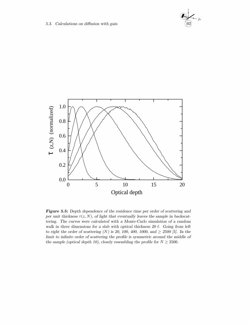
5.3. Calculations on diffusion with gain 93
0 5 10 15 200.0
0.2
0.4
0.6
0.8
1.0
τ(n
orm
aliz
ed)
(z
,N)
Optical depth
Figure 5.5: Depth dependence of the residence time per order of scattering and
per unit thickness τ(z,N), of light that eventually leaves the sample in backscat-
tering. The curves were calculated with a Monte-Carlo simulation of a random
walk in three dimensions for a slab with optical thickness 20 . Going from left
to right the order of scattering (N) is 20, 100, 400, 1000, and ≥ 2500 [5]. In the
limit to infinite order of scattering the profile is symmetric around the middle of
the sample (optical depth 10), closely resembling the profile for N ≥ 2500.
94 Amplifying random media
depth is more important than the excitation of the deeper lying parts ofthe sample.
This can be explained if we consider the average residence time τ(z,N)of light in a layer at depth z in the sample, per order of scattering and perunit of thickness, defined by:
τt ≡∫ ∞∑N=1
τ(z,N) dz, (5.22)
where τt is the total residence time of the light in the sample. In Fig. 5.5, wehave plotted the depth dependence of τ(z,N), for different orders of scat-tering, for light that eventually leaves the sample in backscattering. Goingfrom left to right, the order of scattering for each curve increases wherethe most right curve is almost equal to the limiting case of infinite orderof scattering, which is symmetric around the middle of the sample. We seethat even for very long (finite) paths that leave the sample in the backscat-tering direction, the light spends on average more time in the first half ofthe sample. This explains why the (inhomogeneous) excitation profile ofFig. 5.4 obtained with single sided pumping, yields a larger overall gain,although the average excitation level is lower than for two sided pumping.
5.3.4 Pulsed amplified spontaneous emission
If we look at the temporal behaviour of the excitation in Fig. 5.3, we seethat after the pump pulse, the excitation level is constant over the timewindow in which the probe pulse is present. Here, the excited volume isbelow the critical volume Vcr. If we increase the pump flux and vary thesample thickness, we can reach the critical regime in which the systembecomes unstable. In Fig. 5.6, we have plotted the temporal profile of theamplified spontaneous emission flux in backscattering (W out
A (t)) during andjust after the pump pulse, for various pump fluxes and sample thicknesses.Also plotted, is the pump flux and the temporal profile of the averageexcitation level. Going from left to right, the sample thickness increases,and going from bottom to top, the pump flux doubles in every graph. Wesee that at sufficiently large pump fluxes and (or) large enough samplethicknesses, the outgoing ASE flux is pulsed.
This pulsed behaviour originates from the combination of a diffusionprocess with a time-dependent gain. The relevant length scale to describethe amplification in the system, is the amplification length amp. Duringthe pump pulse, the following process takes place.
5.3. Calculations on diffusion with gain 95
1. In the beginning of the pump pulse, the average amplification lengthin the medium decreases slowly due to the buildup of inversion. The timescale on which this buildup takes place is determined by the pump flux.
2. When amp reaches a critical value (that is, when the critical thicknessgiven by YLcr = π amp, becomes smaller than the sample thickness), the gainin the sample becomes larger than the loss through the boundaries. Thisleads to a large increase of the ASE energy density. The characteristic timescale corresponding to this buildup of ASE is g/v, where g is the gainlength in the medium and v is the (transport) velocity of the light.
3. The situation that π amp < L is unstable. The large ASE energydensity will however de-excite the system, which leads to an increase of amp. This increase continues as long as the large ASE energy density ispresent. The characteristic time scale on which the ASE energy densitydiffuses out of the medium through the front or rear interface, is given byL2/D.
4. The equilibrium situation would be reached when gain equals loss,i.e. when π amp = L. However, if the buildup of a new inversion is slowcompared to L2/D, amp will become larger than L and the process startsall over again.
This process leads to (transient) oscillations in the outgoing ASE flux.Damping of the oscillations occurs due to the fact that the increase of ampin step 3 is opposed by re-excitation due to the presence of pump light. Thesystem reaches therefore after a few oscillations the equilibrium situationπ amp = L.
In Fig. 5.6, the pump flux and the sample thickness is varied. We seethat for larger pump fluxes (going from bottom to top in the graph), theoscillations start earlier and are more rapid, which is due to a more rapiddecrease of amp. We also see that at larger pump fluxes, the equilibriumstate is reached earlier. This is due to a larger damping of the oscillationin step 3. At extremely large pump fluxes, no pulsed output is observedbecause the oscillations become overdamped.
Upon increasing the sample thickness L (going from left to right in thegraph), the oscillations also start earlier because the situation π amp < Lis reached at larger values of amp. The value of amp determines g via
amp =√ g/3. The gain length g is inversely proportional to the excita-
tion level, so the obtained excitation level is in principle inversely propor-tional to the square of the sample thickness. (At large sample thicknesses,the spatial profile of the pump energy density starts to play a role. Thepump light does not penetrate into the deepest layers of the sample dueto absorption, and the sample is therefore effectively thinner than L.) Be-
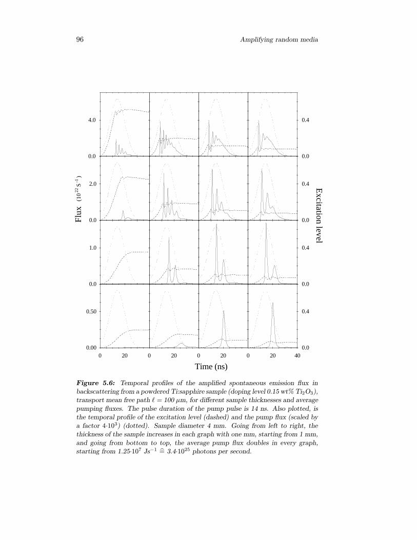
96 Amplifying random media
0.0
4.0
0.0
0.4
0.0
2.0
(10 2
2 S -
1 )F
lux
0.0
0.4 Excitation level
0.0
1.0
0.0
0.4
0 200.00
0.50
0 20 0 20
Time (ns)0 20 40
0.0
0.4
Figure 5.6: Temporal profiles of the amplified spontaneous emission flux in
backscattering from a powdered Ti:sapphire sample (doping level 0.15 wt% Ti2O3),
transport mean free path = 100 µm, for different sample thicknesses and average
pumping fluxes. The pulse duration of the pump pulse is 14 ns. Also plotted, is
the temporal profile of the excitation level (dashed) and the pump flux (scaled by
a factor 4·103) (dotted). Sample diameter 4 mm. Going from left to right, the
thickness of the sample increases in each graph with one mm, starting from 1 mm,
and going from bottom to top, the average pump flux doubles in every graph,
starting from 1.25·107 Js−1 = 3.4·1025 photons per second.
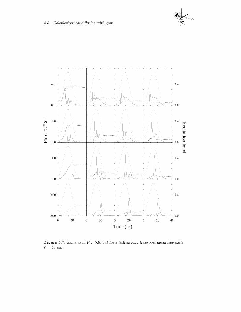
5.3. Calculations on diffusion with gain 97
0.0
4.0
0.0
0.4
0.0
2.0
(10 2
2 S -
1 )F
lux
0.0
0.4 Excitation level
0.0
1.0
0.0
0.4
0 200.00
0.50
0 20 0 20
Time (ns)0 20 40
0.0
0.4
Figure 5.7: Same as in Fig. 5.6, but for a half as long transport mean free path:
= 50 µm.
98 Amplifying random media
cause the characteristic time scale for the buildup of ASE is g/v, and thetimescale for the diffusion out of the sample is L2/D, oscillations becomeslower at larger sample thickness. This again leads to the fact that theequilibrium state is reached earlier.
In Fig. 5.7, the same graph is plotted as in Fig. 5.6 but now for a halfas long transport mean free path . Because amp is proportional to thesquare root of , a decrease of leads to an earlier onset of the oscillations.This again leads to larger values of g and correspondingly smaller valuesof the excitation level. Due to a larger g and a smaller diffusion constant(D = 1
3v ), the oscillations are slower and the equilibrium state is reachedearlier.
Concluding we can say, that powdered laser materials can show a pulsedoutput depending on various experimental parameters. This pulsed be-haviour is due to the combination of a diffusion ‘loss’ process and a time-dependent gain process. The consequence for realizing amplifying randommedia is, that the pump parameters must be chosen with care. Largelyincreasing the pump flux does not necessarily lead to a considerably largergain coefficient in the medium.
5.4 Random lasers
The output of an amplifying random medium can show characteristics thatare very similar to laser action. The output can be spectrally narrow andpulsed. It is tentative to call this system a random laser, however one has tobe careful. It is important to distinguish three different regimes of multiplescattering with gain, depending on the strength of the scattering.
Very weak scattering and gain
If the scattering is very weak, that is is of the order of the sample size, therole of the scatterers is to scramble the directionality of the light emitted bythe laser material. If we pump a clear laser material in a certain geometry,ASE will build up in the direction of largest gain, which is generally thedirection in which the excited region is most extended. This yields a direc-tionality in the output of the system. Due to gain narrowing, the spectrumof ASE can be very narrow like the output of a laser. Also, due to the buildup of ASE, the temporal behaviour of the emission can be very rapid. Thepulse length of ASE can be much shorter than the lifetime of the excitedstate of the laser material, but is always equal to or larger than the pumppulse length. If one adds some scatterers to the clear laser material, the
5.4. Random lasers 99
directionality of the ASE is scrambled, and in all directions the output willbe narrow banded and will decay rapidly. In Ref. [6] this effect was mistak-enly interpreted as random laser action (see Ref. [7]). If one monitors theemitted light in a direction in which the excited clear laser material showsno ASE, the introduction of some scatterers will result in a narrowing ofthe observed spectrum (see Fig. 5.8), and a shortening of the pulse lengthof the emission (see Fig. 5.9). In this regime of very weak scattering, theonly role of the particles is to scramble the directionality of the ASE, whichbuilds up (also in the absence of scatterers) in the excited laser material.
Weak scattering and gain
If the scattering is stronger so that is much smaller than the sample sizebut still larger than the wavelength, we are in the regime where the scat-terers influence the spectrum of the output. In this regime, ASE buildsup along random paths in the sample that are much longer than the di-rection in which the sample is most extended. This means that due tothe scattering process, ASE can build up in a laser material that wouldshow no ASE without scatterers. Here the scattering contributes to gainnarrowing, because it largely increases the residence time of the light in thesample. This also leads to a pulsed output, as we found in section 5.3, andin this case the pulse duration of the ASE can be shorter than the pumppulse length. This pulsed output was also observed in Ref. [8], where theemission characteristics from powdered laser crystals were studied.
In the above described situation of weak scattering with gain, the scat-tering process induces a narrow spectrum and pulsed output. Thereforeit is tempting to call this effect random laser action. However, to achievelaser action, some feedback mechanism is required. In a laser, the cavitymirrors provide this feedback mechanism. Due to this feedback, lasing onlyoccurs in the spatial modes allowed by the cavity. In the weak scatter-ing regime, the light waves perform a random walk without returning to aspecific scatterer, so there is no feedback.
Strong scattering and gain
The feedback mechanism which is essential for a laser oscillator, could beprovided by recurrent scattering events that occur, as we have shown inchapter 4, in the strong scattering regime for k <∼ 10. If the amplificationalong a recurrent light path would be strong enough, these recurrent (looptype) paths could serve as ring cavities for the light. In that case the systemwould lase in the modes allowed by these random ring cavities. This we
100 Amplifying random media
would call random laser action.If we consider a system in which the amplification does not take place
inside the particles but in between two scattering events (e.g. a medium thatconsists of TiO2 particles suspended in a laser dye solution), the waves donot have to return to a specific scatterer to attain optical feedback. Thecriterium for a feedback mechanism then becomes whether waves return toa certain position in the amplifying medium surrounding the scatterers.
From an experimental point of view, it is difficult to obtain strong scat-tering and amplification. One option would be to dope TiO2 particles withe.g. a Rhodamine laser dye. The disadvantage of such a system is that thelifetime of the excited state is very short (see section 5.2), and experimentshave to be performed with picosecond time resolution. Another optionis to mix a strongly scattering medium like TiO2 powder with powderedTi:sapphire. In that case however, the presence of Ti:sapphire particlesreduces the scattering strength compared to a pure TiO2 powder.
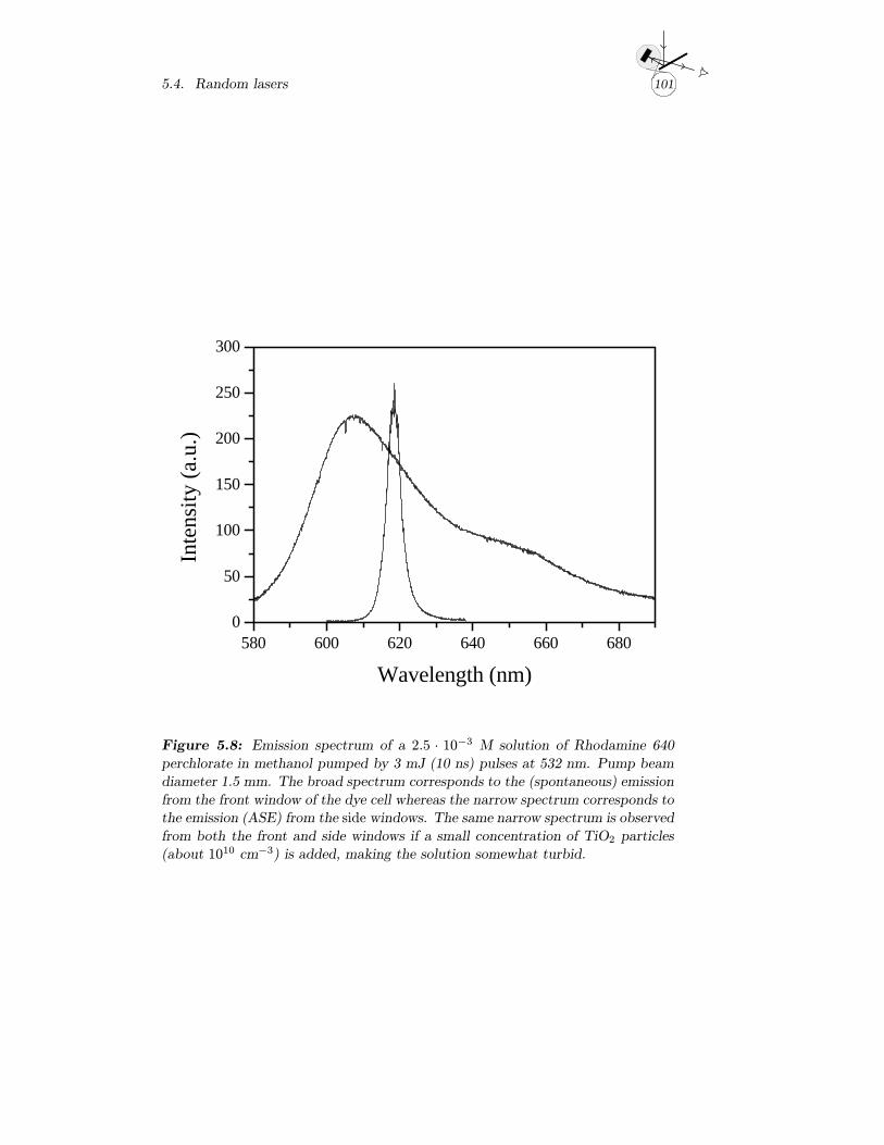
5.4. Random lasers 101
580 600 620 640 660 6800
50
100
150
200
250
300
Inte
nsity
(a.
u.)
Wavelength (nm)
Figure 5.8: Emission spectrum of a 2.5 · 10−3 M solution of Rhodamine 640
perchlorate in methanol pumped by 3 mJ (10 ns) pulses at 532 nm. Pump beam
diameter 1.5 mm. The broad spectrum corresponds to the (spontaneous) emission
from the front window of the dye cell whereas the narrow spectrum corresponds to
the emission (ASE) from the side windows. The same narrow spectrum is observed
from both the front and side windows if a small concentration of TiO2 particles
(about 1010 cm−3) is added, making the solution somewhat turbid.
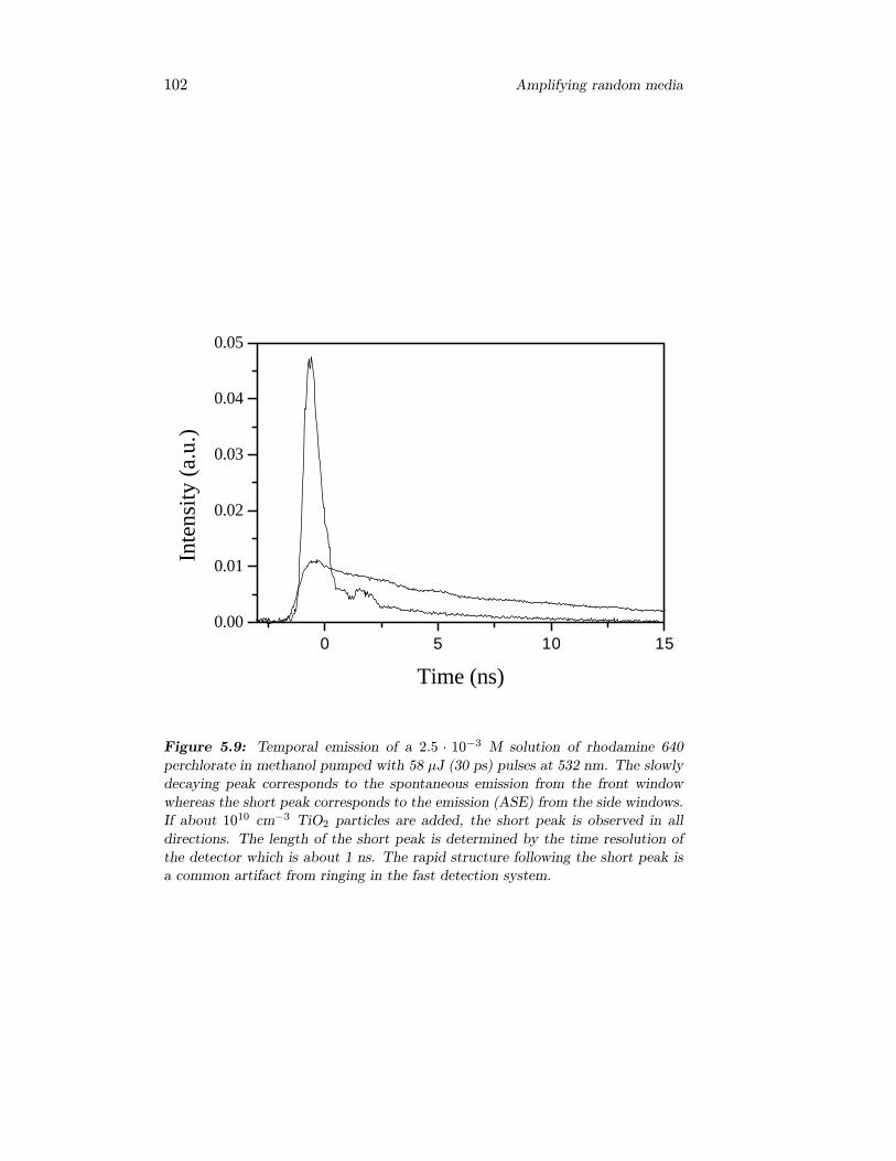
102 Amplifying random media
0 5 10 150.00
0.01
0.02
0.03
0.04
0.05
Inte
nsity
(a.
u.)
Time (ns)
Figure 5.9: Temporal emission of a 2.5 · 10−3 M solution of rhodamine 640
perchlorate in methanol pumped with 58 µJ (30 ps) pulses at 532 nm. The slowly
decaying peak corresponds to the spontaneous emission from the front window
whereas the short peak corresponds to the emission (ASE) from the side windows.
If about 1010 cm−3 TiO2 particles are added, the short peak is observed in all
directions. The length of the short peak is determined by the time resolution of
the detector which is about 1 ns. The rapid structure following the short peak is
a common artifact from ringing in the fast detection system.
103
References and notes
[1] Note that the term photon is used to denote a classical energy packetand does not refer to a quantization of the light field.
[2] M.P. van Albada, B.A. van Tiggelen, A. Lagendijk, and A. Tip, Phys.Rev. Lett. 66, 3132 (1991).
[3] A. Bott and W. Zdunkowski, J. Opt. Soc. Am. A4, 1361 (1987).[4] W.H. Press, B.P. Flannery, S.A. Teukolsky, and W.T. Vetterling, Nu-
merical Recipies (Cambridge University Press, 1989).[5] The last curve (for N ≥ 2500) is the summation of τ(z,N) over N =
2500 . . . ∞.[6] N.M. Lawandy, R.M. Balachandran, A.S.L. Gomes, and E. Sauvain,
Nature 368, 436 (1994).[7] D.S. Wiersma, M.P. van Albada, and A. Lagendijk, Nature 373, 203
(1995).[8] C. Gouedard, D. Husson, C. Sauteret, F. Auzel, and A. Migus, J. Opt.
Soc. Am. B 10, 2358 (1993).

104
Chapter 6
Experiments on randommedia with gain
6.1 Introduction
The availability of amplifying random media as described in chapter 5,allows to study multiple scattering (interference) phenomena in active me-dia. The experimental studies on multiple light scattering so far, have beenrestricted mostly to passive and linear random media. One nonlinear ex-perimental study was performed on powdered LiNbO3 crystals [1], wherespatial correlations of second harmonic waves were studied. This systemwas nevertheless still a passive medium.
Much interest is shown recently in performing coherent experiments onactive, amplifying random media. In a recent paper by Lawandy et al. lasereffects were reported from suspensions of latex microspheres in laser dyesolutions [2], but the reported phenomenon is not induced by scattering(see section 5.4). Recently it was shown by Gouedard et al. that powderedlaser crystals can serve as incoherent quasi monochromatic light sources [3].No coherent multiple scattering experiments have been performed yet onamplifying random media.
The behaviour of an amplifying random medium is expected to be differ-ent from that of an (absorbing) passive one. Since the amplification alonga light path depends on the path length, the overall scattering propertiesdepend strongly on the sample size. As explained in section 5.1.1, there isfor instance a critical sample size, above which the intensity diverges andthe system becomes unstable. In that sense, multiple light scattering withgain is similar to neutron scattering in combination with nuclear fission [4].
105
106 Experiments on random media with gain
In this chapter, we will discuss experiments on laser speckle and coher-ent backscattering from an amplifying random medium. Both experiments,are a demonstration of the combination of a multiple scattering interferenceeffect with optical amplification.
6.2 Laser speckle
When coherent laser light is scattered by a random collection of particlesor even a rough surface, the angular dependence of the scattered intensityshows strong fluctuations known as laser speckle [5]. These fluctuationsare of the order of the average scattered intensity, and at some angles thescattered intensity is truly zero. This effect is due to interference between(multiply) scattered waves.
A speckle pattern that is recorded in transmission from a random col-lection of particles, is very sensitive to the relative positions of the particles.The pattern changes completely if the particles move over a distance muchsmaller than the wavelength. The change of phase of a scattered wave isdue to the motion of all particles from which this wave is scattered. If awave is scattered by N particles, its phase will change significantly if eachparticle moves over a distance of only 1/N times the wavelength. This ef-fect is used to study the motion of particles on a length scale much smallerthan the wavelength, in a technique called ‘Diffusing-Wave Spectroscopy’[6].
One can model a random sample as a waveguide that couples incidentwaves from incoming modes α and α′ to outgoing modes β and β′. Fora random sample, a mode is a solid angle containing one coherence area(i.e. one speckle spot). The intensity transmission coefficient from incomingmode α to outgoing mode β is denoted by Tαβ. The correlation betweenthe intensities in different modes is given by: Cαβα′β′ = 〈δTαβ δTα′β′〉 withδTαβ = (Tαβ − 〈Tαβ〉)/〈Tαβ〉, where angular brackets denote an averageover different configurations of the sample. The correlator Cαβα′β′ con-sists of three terms describing short range, long range, and ‘infinite range’correlations [7]. We will not discuss these correlations in this thesis.
If one wants to study the mode properties of an amplifying medium—for instance, if one wants to realize and study a ‘random laser’— it isimportant that the particles are stationary over a length scale much smallerthan the wavelength. One can expect that the large intensities requiredto excite the laser material, will locally heat up the sample and inducestructural changes that average out the speckle pattern.
6.2. Laser speckle 107
6.2.1 Experimental configuration and results
The outline of the setup is relatively simple. A powdered Ti:sapphire sam-ple is pumped with intense pulses from a frequency doubled Nd:YAG laser(wavelength 532 nm, pulse duration 14 ns, repetition rate 10 Hz). Witha time delay of 14 ns after the pump pulse, a low intensity probe pulseis incident on the sample (wavelength 780 nm, pulse duration 14 ns, pulseenergy 85 µJ). The transmitted probe light is recorded with an optical fiber(core diameter 50 µm) at a distance of 40 cm from the sample, which cor-responds to a solid angle of detection of 125 µrad. The scattered intensityat a fixed position is recorded while the sample rotates. This way, both theincoming and outgoing angle are varied at the same time [8]. This is a ‘onemode in, one mode out’ type of experiment, because the light is incidentin one direction, and the solid angle of detection is smaller than the size ofone speckle spot.
The diameter of the probe beam is about 200 µm. Pump and probebeam are incident on the same side of the sample. The sample has aslab geometry with a thickness of about 100 µm, and consists of powderedTi:sapphire (doping level 0.15 wt% Ti2O3). The particles are strongly poly-disperse and have an average diameter of 10 µm. The preparation of thesamples is described in section 6.3.1.
The pulse energy of the pump light was varied between 0 and 100 mJ,and the diameter of the pump beam was varied between 4 and 6 mm.The pump beam was blocked at every second shot and the probe signalobtained this way without pump light, was averaged separately to serve asa reference measurement. The detected probe signal was averaged over 25laser shots. In Fig. 6.1, the transmitted probe intensity is plotted versus therotation angle of the sample. The solid line corresponds to a pump energyof 98 mJ, at a beam diameter of 7.5 mm, which corresponds to a pumpintensity of 1.6·1011 J/m2s. The dotted line is the reference measurementwithout pump light. The overall gain (i.e. the average gain over all angles)of the measurement with pump light is 18 %. We see that the introduc-tion of gain does not change the observed pattern to a large extend. Thisbehaviour is found for various measurements at low pump intensities. Ifwe decrease the diameter of the pump beam to 5 mm at the same pulseenergy (corresponding to a pump intensity of 2.4·1011 J/m2s), the observedpattern changes completely (see Fig. 6.2). This pump intensity is close tothe damage threshold of the sample, which lies about a factor 2 - 3 abovethis intensity.
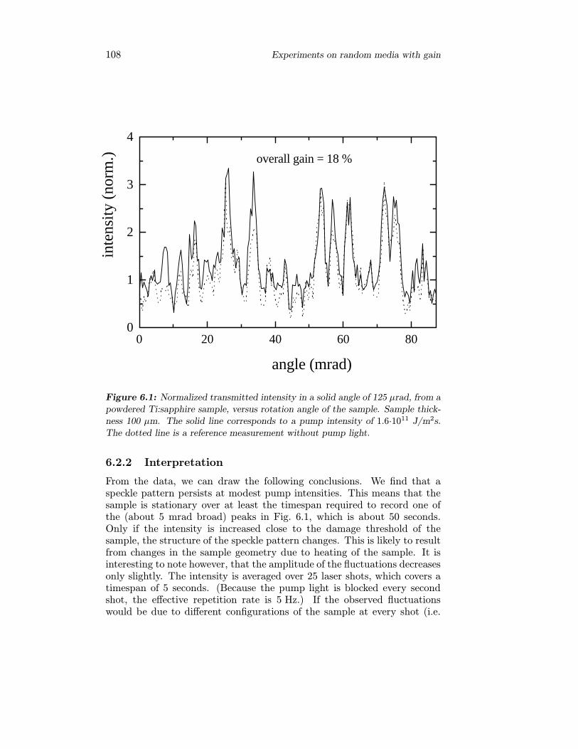
108 Experiments on random media with gain
0 20 40 60 800
1
2
3
4
overall gain = 18 %
inte
nsity
(no
rm.)
angle (mrad)
Figure 6.1: Normalized transmitted intensity in a solid angle of 125 µrad, from a
powdered Ti:sapphire sample, versus rotation angle of the sample. Sample thick-
ness 100 µm. The solid line corresponds to a pump intensity of 1.6·1011 J/m2s.
The dotted line is a reference measurement without pump light.
6.2.2 Interpretation
From the data, we can draw the following conclusions. We find that aspeckle pattern persists at modest pump intensities. This means that thesample is stationary over at least the timespan required to record one ofthe (about 5 mrad broad) peaks in Fig. 6.1, which is about 50 seconds.Only if the intensity is increased close to the damage threshold of thesample, the structure of the speckle pattern changes. This is likely to resultfrom changes in the sample geometry due to heating of the sample. It isinteresting to note however, that the amplitude of the fluctuations decreasesonly slightly. The intensity is averaged over 25 laser shots, which covers atimespan of 5 seconds. (Because the pump light is blocked every secondshot, the effective repetition rate is 5 Hz.) If the observed fluctuationswould be due to different configurations of the sample at every shot (i.e.
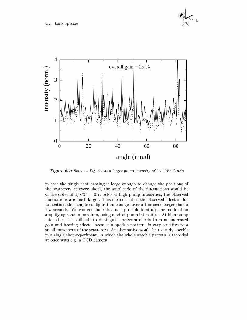
6.2. Laser speckle 109
0 20 40 60 800
1
2
3
4overall gain = 25 %
inte
nsity
(no
rm.)
angle (mrad)
Figure 6.2: Same as Fig. 6.1 at a larger pump intensity of 2.4· 1011 J/m2s
in case the single shot heating is large enough to change the positions ofthe scatterers at every shot), the amplitude of the fluctuations would be
of the order of 1/√25 = 0.2. Also at high pump intensities, the observed
fluctuations are much larger. This means that, if the observed effect is dueto heating, the sample configuration changes over a timescale larger than afew seconds. We can conclude that it is possible to study one mode of anamplifying random medium, using modest pump intensities. At high pumpintensities it is difficult to distinguish between effects from an increasedgain and heating effects, because a speckle patterns is very sensitive to asmall movement of the scatterers. An alternative would be to study specklein a single shot experiment, in which the whole speckle pattern is recordedat once with e.g. a CCD camera.
110 Experiments on random media with gain
6.3 Coherent backscattering
As explained in chapter 2, coherent backscattering is a general interferenceeffect for waves which are backscattered from a random medium. It leads toa cone of enhanced backscattering in and around the exact backscatteringdirection, which usually has a width of the order of a few mrad. Coherentbackscattering is an example of a multiple scattering interference effect.It is of particular interest because the (top of the) backscattering cone isdue to very long light paths that have penetrated deep into the sample.Theoretically, paths of infinite length contribute to the cusp in the top ofthe backscattering cone. In practice, features due to > 104 scattering eventsare experimentally accessible. Because very long light paths contribute tothe top of cone, we expect coherent backscattering to be strongly influencedby gain.
In the following, we will describe coherent backscattering experimentson samples of powdered Ti:sapphire. We found in chapter 5, that suchsamples can yield a (relatively large) gain of more than 150 %. Also we willshow how diffusion theory can be used to calculate the angular dependenceof the backscattered light from an amplifying random medium.
6.3.1 Samples
The samples consist of powdered Ti:Sapphire crystals. These powders wereprepared by grinding Ti:Sapphire laser rods [10] for about 5 min. in aplanetary micromill. The samples are strongly polydisperse with an averageparticle size of 10 µm. The (transport) mean free path was varied between18 and 40 µm, by using both dry Ti:sapphire powders and suspensions ofTi:sapphire powder in water. The samples have a slab geometry, withthickness 1 mm and diameter 15 mm. The powders and suspensions arecontained in a sample cell with a thick (1 cm) slightly wedged window,anti-reflection coated on the front side. Great care was taken to preparethe samples as clean as possible, because we found that any impurity thatabsorbs light at the pump wavelength, causes the sample to ‘explode’. Thatis, the single shot heating of the sample around an impurity is large enoughto cause serious structural damage to the sample. The long term heatingof the sample due to the intense pump light was however less than 10 K.
6.3.2 Setup
The outline of the setup is drawn in Fig. 6.3. The Ti:Sapphire is optical-ly pumped through the front sample interface with a frequency doubled
6.3. Coherent backscattering 111
Nd:YAG laser (wavelength 532 nm) with pulse energies varying between 0and 190 mJ. After a time delay of 14 ns, the green pump pulse is followedby a low intensity red probe pulse (wavelength 780 nm). The beams co-incide spatially on the sample surface and both have a diameter of 5 mm.The angular distribution of the scattered probe light is recorded using theoff-centered rotation setup as described in chapter 3. In this setup, anoptical fiber and a photo multiplier tube are used to record the scatteredprobe light. The probe light is linearly polarized and both the polarizationconserving and reversing channel have been monitored.
To record a backscattering cone, an average must be taken over manyconfigurations of the sample, to eliminate the spatial speckle pattern whichis always formed if a coherent beam is scattered from a (stationary) sample.To that end, the sample is rotated slowly around its axis. Because we usea pulsed probe beam with a pulse duration of 14 ns, the sample is almostcompletely stationary over the time window of one probe pulse. This meansthat the average over different sample configurations is performed with therepetition rate of the probe, which is 10 Hz. If we follow the rule of thumbthat the relative fluctuations on the signal due to speckle are of the order ofN−1/2, with N the number of sample realizations, we have to average overN = 10000 probe shots to obtain a speckle noise level of 1 %. This leadsto measurement times in the order of hours, to record a backscatteringcone. To be able to correct for artifacts from e.g. cumulative heating ofthe sample or long term drift, the pump beam is blocked at every othershot. This way, the sample is pumped just before every second probe pulseonly. The detected signals from even and odd probe pulses are averagedseparately, so one experimental run yields one backscattering cone withgain, and one reference cone without gain.
The setup has to be aligned such that an angular scan passes throughthe top of the backscattering cone, which requires an accuracy of about100 µrad both in the plane of the angular scan and perpendicular to it.This alignment is more difficult using pulsed light at a low repetition rate,which is also due to the large number of probe pulses over which one hasto average. To facilitate this procedure, a CCD array is mounted close tothe optical fiber (see Fig. 6.3). The CCD signal is stored and averaged overseveral frames. Alignment of the top of the cone on the center of the CCDarray is considerably easier than alignment of the top on the head of theoptical fiber. After alignment on the CCD array, the setup can be rotatedover a (known) angle such that the top of the backscattering cone is alignedon the fiber. The CCD array could not be used to record backscatteringcones with gain, because for these measurements, the detector must begated on a nanosecond timescale (see below).
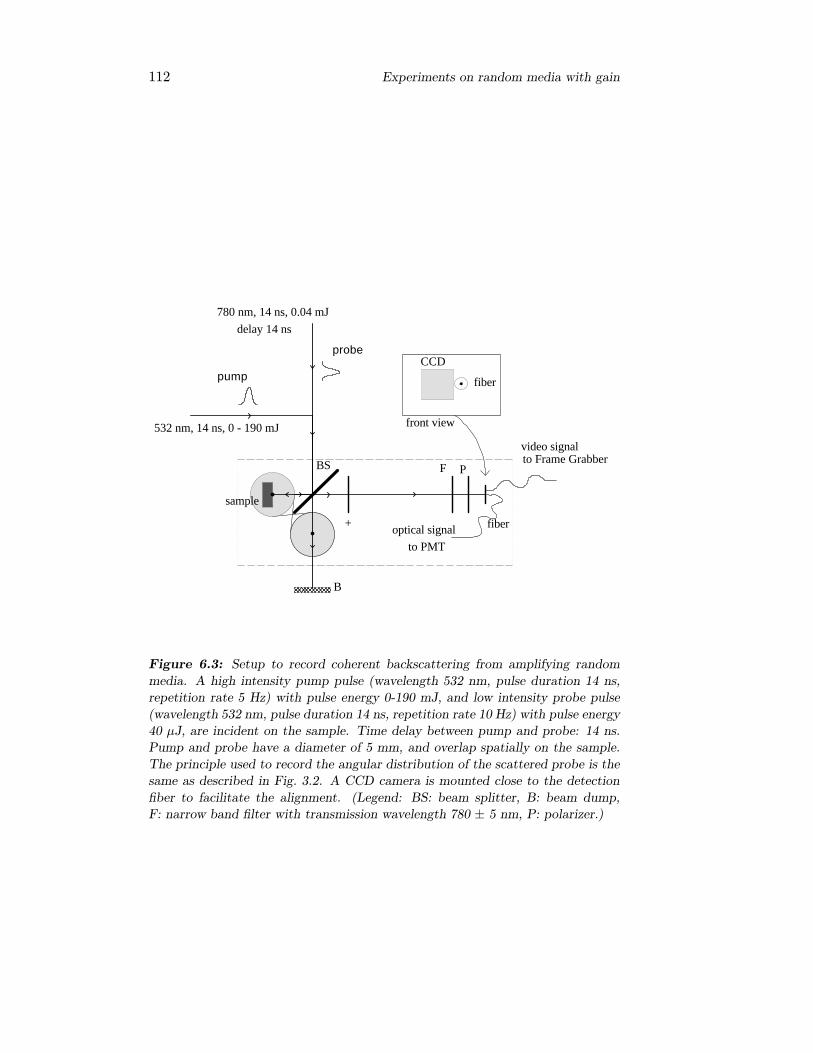
112 Experiments on random media with gain
+
to PMT
PBS
B
fiber
sample
to Frame GrabberF
video signal
optical signal
532 nm, 14 ns, 0 - 190 mJ
780 nm, 14 ns, 0.04 mJ
delay 14 ns
CCD
fiber
front view
pump
probe
Figure 6.3: Setup to record coherent backscattering from amplifying random
media. A high intensity pump pulse (wavelength 532 nm, pulse duration 14 ns,
repetition rate 5 Hz) with pulse energy 0-190 mJ, and low intensity probe pulse
(wavelength 532 nm, pulse duration 14 ns, repetition rate 10 Hz) with pulse energy
40 µJ, are incident on the sample. Time delay between pump and probe: 14 ns.
Pump and probe have a diameter of 5 mm, and overlap spatially on the sample.
The principle used to record the angular distribution of the scattered probe is the
same as described in Fig. 3.2. A CCD camera is mounted close to the detection
fiber to facilitate the alignment. (Legend: BS: beam splitter, B: beam dump,
F: narrow band filter with transmission wavelength 780 ± 5 nm, P: polarizer.)
6.3. Coherent backscattering 113
A problem that arises in scattering experiments on pumped laser ma-terials, is that one has to distinguish between the scattered probe lightand (amplified) spontaneously emitted light. Usually the bandwidth of theprobe light is (much) smaller than the spectral width of the spontaneousemission. Therefore, a narrow band interference filter at the wavelength ofthe probe light is mounted in front of the detector. Furthermore, the timedependence of probe light and (amplified) spontaneous emission is usuallyvery different. If the excited region in the sample is much smaller than thecritical volume (see section 5.3), the characteristic time of the (amplified)spontaneous emission is close to the lifetime of the excited state of thelaser material. The lifetime of the excited state of Ti:Sapphire is 3.2 µs.By monitoring the scattered light only during a limited time window of afew nanoseconds, the fraction of detected (amplified) spontaneous emissionbecomes negligible. This was done electronically by storing the oscilloscopetrace of the PMT signal, and subsequently averaging the signal over thetime window of 14 ns in which the probe is present.
6.3.3 Results
In Fig. 6.4, backscattering cones are shown as recorded for the same sampleat different pump energies. The probe was linearly polarized and the po-larization conserving channel was monitored. The solid line is a theoreticalcurve calculated with diffusion theory. We will describe this calculationin the next section. We see that the overall scattered intensity increaseswith pump energy. The pump energies for these data were 0, 165, and 190mJ, which yields an overall gain of resp. 0, 36, and 71 %. We also seethat the shape of the cone changes: upon increasing the gain, the top ofthe backscattering cone sharpens. This sharpening becomes even moreapparent if the y-axis is scaled such that the background levels coincide,which is shown in Fig. 6.5. From Fig. 6.5 we also see that the enhancementfactor is essentially independent of the gain.
In Fig. 6.6, the backscattering cone is shown from the same sample as inFig. 6.4, monitoring the polarization reversing channel. We see that in thepolarization reversing channel even without gain, the enhancement factorof the backscattering cone of these samples is too small to distinguish acone from the diffuse background.
6.3.4 Interpretation
The narrowing of the top of the backscattering cone in the polarizationconserving channel, can be understood if one realizes that the shape of
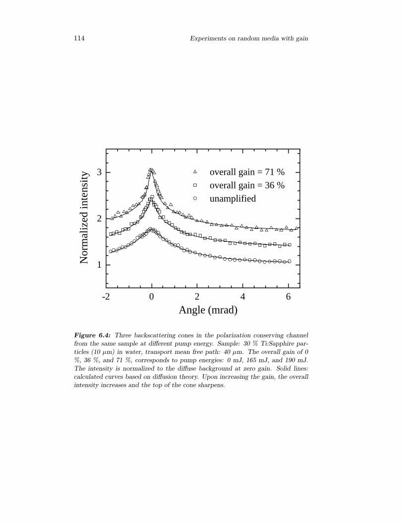
114 Experiments on random media with gain
-2 0 2 4 6
1
2
3 overall gain = 71 % overall gain = 36 % unamplified
Nor
mal
ized
inte
nsity
Angle (mrad)
Figure 6.4: Three backscattering cones in the polarization conserving channel
from the same sample at different pump energy. Sample: 30 % Ti:Sapphire par-
ticles (10 µm) in water, transport mean free path: 40 µm. The overall gain of 0
%, 36 %, and 71 %, corresponds to pump energies: 0 mJ, 165 mJ, and 190 mJ.
The intensity is normalized to the diffuse background at zero gain. Solid lines:
calculated curves based on diffusion theory. Upon increasing the gain, the overall
intensity increases and the top of the cone sharpens.
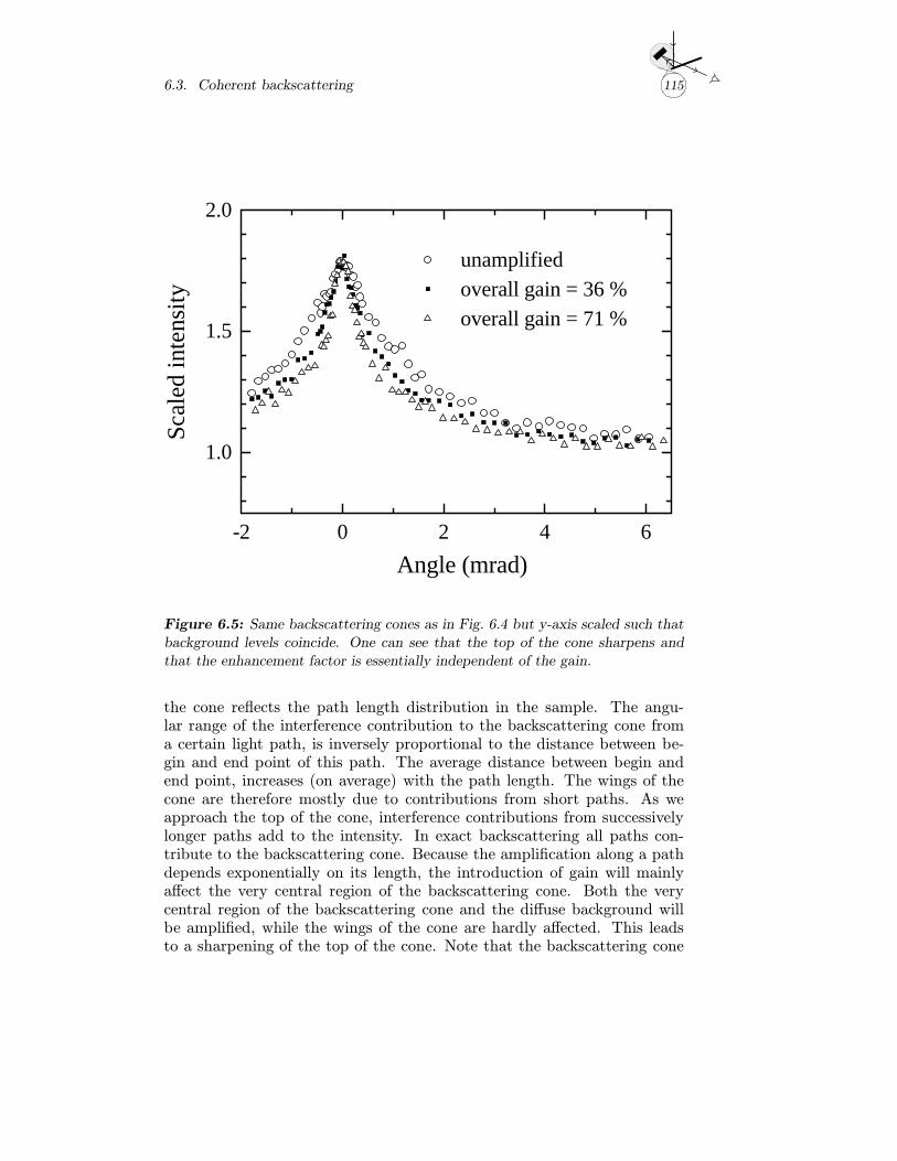
6.3. Coherent backscattering 115
-2 0 2 4 6
1.0
1.5
2.0
unamplified overall gain = 36 % overall gain = 71 %
Scal
ed in
tens
ity
Angle (mrad)
Figure 6.5: Same backscattering cones as in Fig. 6.4 but y-axis scaled such that
background levels coincide. One can see that the top of the cone sharpens and
that the enhancement factor is essentially independent of the gain.
the cone reflects the path length distribution in the sample. The angu-lar range of the interference contribution to the backscattering cone froma certain light path, is inversely proportional to the distance between be-gin and end point of this path. The average distance between begin andend point, increases (on average) with the path length. The wings of thecone are therefore mostly due to contributions from short paths. As weapproach the top of the cone, interference contributions from successivelylonger paths add to the intensity. In exact backscattering all paths con-tribute to the backscattering cone. Because the amplification along a pathdepends exponentially on its length, the introduction of gain will mainlyaffect the very central region of the backscattering cone. Both the verycentral region of the backscattering cone and the diffuse background willbe amplified, while the wings of the cone are hardly affected. This leadsto a sharpening of the top of the cone. Note that the backscattering cone
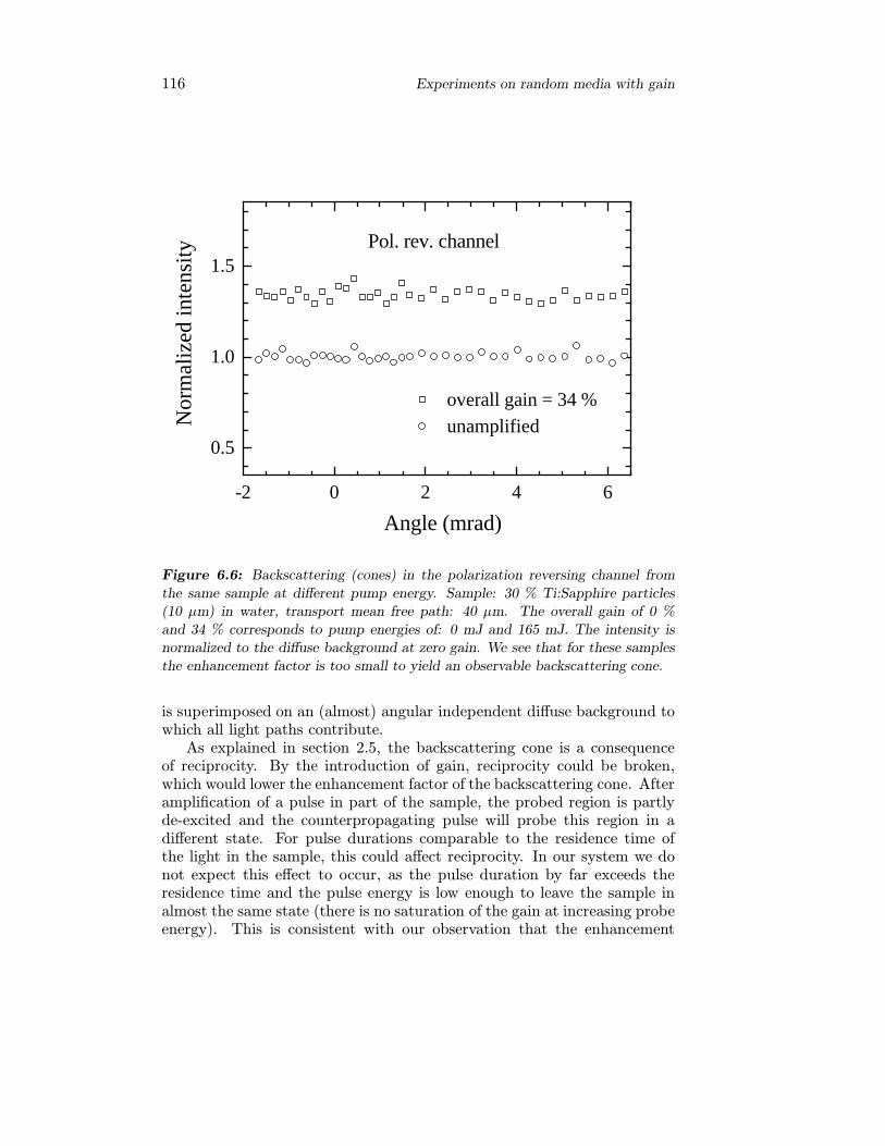
116 Experiments on random media with gain
-2 0 2 4 6
0.5
1.0
1.5Pol. rev. channel
overall gain = 34 %unamplifiedN
orm
aliz
ed in
tens
ity
Angle (mrad)
Figure 6.6: Backscattering (cones) in the polarization reversing channel from
the same sample at different pump energy. Sample: 30 % Ti:Sapphire particles
(10 µm) in water, transport mean free path: 40 µm. The overall gain of 0 %
and 34 % corresponds to pump energies of: 0 mJ and 165 mJ. The intensity is
normalized to the diffuse background at zero gain. We see that for these samples
the enhancement factor is too small to yield an observable backscattering cone.
is superimposed on an (almost) angular independent diffuse background towhich all light paths contribute.
As explained in section 2.5, the backscattering cone is a consequenceof reciprocity. By the introduction of gain, reciprocity could be broken,which would lower the enhancement factor of the backscattering cone. Afteramplification of a pulse in part of the sample, the probed region is partlyde-excited and the counterpropagating pulse will probe this region in adifferent state. For pulse durations comparable to the residence time ofthe light in the sample, this could affect reciprocity. In our system we donot expect this effect to occur, as the pulse duration by far exceeds theresidence time and the pulse energy is low enough to leave the sample inalmost the same state (there is no saturation of the gain at increasing probeenergy). This is consistent with our observation that the enhancement
6.3. Coherent backscattering 117
factor is essentially independent of the gain (Fig. 6.5).In the polarization reversing channel, the backscattering cones from
our samples did not exhibit a significant enhancement factor (Fig. 6.6).In the polarization reversing channel, correlation between the amplitudesand phases of counterpropagating waves diminishes with increasing order ofscattering [11]. Coherent backscattering in this channel is due to low orderscattering (short paths). Depending on the phase function of the scatter-ers, the enhancement factor ranges from 1.0 to about 1.2. We expect thisenhancement factor to decrease with gain because long path contributionsare only present in the background and not in the cone. Apparently oursamples exhibit an enhancement factor smaller than 1.05, which does notallow to measure this dependence of the enhancement factor on gain.
6.3.5 Theory
In chapter 3, we found that the backscattering cone calculated in the diffu-sion approximation, provides a very good description of coherent backscat-tering from passive random media. In the following we will use diffusiontheory to calculate the backscattered intensity from an amplifying randommedium. We start from the stationary diffusion equation with gain [4,12]:
13 2∇2r1F (r1, r2) + κg F (r1, r2) = − δ(r1 − r2). (6.1)
Here F (r1, r2) is the intensity Green’s function, κg is the gain coefficientin the medium, and is the (transport) mean free path. We assume κg tobe position-independent.
If we use a slab geometry, the appropriate boundary condition isF (r1, r2) = 0 in planes at distance z0 on both sides of the slab, withz0 ≈ 0.71 [13]. In the conventional way of solving a diffusion equation withthese boundary conditions (used in e.g. Ref. [14] to calculate the backscat-tering cone from a passive random medium with a slab geometry), thediffusion propagator F (r1, r2) is first calculated for an infinite medium.Subsequently, the boundary conditions for the slab are fulfilled by multi-ple reflections of F (r1, r2) in ‘mirror planes’ on both sides of the slab [15].(These ‘mirror planes’ are also referred to as ‘trapping planes’.) This pro-cedure can not be followed for an amplifying medium, because the diffusionpropagator F (r1, r2) for an infinite amplifying random medium, divergesfor |r1 − r2|→ ∞. Because we have to calculate the angular dependence ofthe backscattered intensity, we wish to perform a Fourier transform of the
118 Experiments on random media with gain
form:
F (q⊥, z1, z2) =
∫F (r1, r2)e
ir⊥·q⊥dr⊥, (6.2)
with r⊥ = r1⊥ − r2⊥ perpendicular to z, where the slab is oriented inthe xy-plane. Here q⊥ is the perpendicular component of the outgoingwavevector. The integral has to be performed over the whole surface of theslab, and diverges because F (r1, r2) diverges for r⊥ →∞.
The solution to this problem is to perform the Fourier transformationon the original diffusion equation (6.1), before the boundary conditions areapplied. The diffusion equation then reads:
13 2(∂2
∂z21− q2⊥
)F (q⊥, z1, z2) + κgF (q⊥, z1, z2) + δ(z1 − z2) = 0. (6.3)
The boundary condition now is: F (q⊥, z1, z2) = 0 for z2 = −z0 and z2 =L + z0, and for every z1. Solving Eq. (6.3) with this boundary conditionwe find:
F (q⊥, z1, z2) = F (q⊥, zs, zd) =3 cos(β(L− zs))− 3 cos(β(L+ 2z0 − |zd|))
2 2 β sin(β(L+ 2z0)),
(6.4)where zs ≡ z1 + z2, zd ≡ z1 − z2, L is the slab thickness, and
β ≡√ −2amp − q2⊥, (6.5)
with amp the amplification length in the medium. The amplification lengthis defined as the (rms) average distance over which the intensity is amplifiedin the medium by a factor e+1.
From Eq. (6.4) we can see that F (q⊥, z1, z2) becomes unstable (thatis diverges for small angles) for L + 2z0 ≥ Lcr = π amp, where Lcr is thecritical thickness. In practice, if we try to make the amplifying region ina slab of disordered laser material thicker than Lcr, the gain will saturateclose to L = Lcr, which provides an upper limit for the intensity.
With the solution for the diffusion propagator F (q⊥, z1, z2) for a slabgeometry, we can calculate the backscattering cone in the same way as wasdescribed in section 2.4 for a passive random medium. From Eq. (2.47),we can derive the following expression for the bistatic coefficient describing
6.3. Coherent backscattering 119
the backscattering cone:
γc(θs) =1
∫ L0
∫ 2L−zdzd
F (q⊥, z1, z2) cos(zdη)e−uzsdzsdzd, (6.6)
where η ≡ k0(1 − µs), u ≡12κe(1 + µ−1s ), and µs = cos(θ) with θ is the
angle of the outgoing wavevector k2 relative to the z-axis. Here κe is theextinction coefficient given by κe = −1s − −1g , where s is the scatteringmean free path and g is the gain length in the medium. The incomingwavevector is taken along the z-axis.
The integrals in Eq. (6.6) can be performed explicitly using the intensitypropagator from Eq. (6.4). The result is:
γc(θs) =3e−uL
2 3β sin[β(L+ 2z0)]
1
(β2 + η2 + u2)2 − (2βη)2× (6.7)
[2(β2 + η2 + u2) cos(2βz0) cos(Lη)− 4βη sin(2βz0) sin(Lη)
+2β
u(−β2 + η2 − u2) sin(β(L+ 2z0)) sinh(uL)
+2(β2− η2− u2) cos(Lη) − 2(β2 + η2 + u2) cos(β(L+ 2z0)) cosh(uL)
+4βu sin(βL) sinh(uL) + 2(−β2 + η2 + u2) cos(βL) cosh(uL)].
In this expression, η, u, and β depend on the scattering angle θ. For smallangles, this solution agrees with the results of Ref. [16], in which coherentbackscattering from an amplifying medium was calculated, but in which anunnecessary approximation was made which makes their result only validfor the central region around the cusp of the cone. For passive media,usually the limit L→∞ is taken to obtain a much simpler expression. Foramplifying media this is impossible due to the divergence of the intensityfor L > Lcr.
It is instructive to compare the backscattering cone with gain to thecone from a passive medium. To that end, we can look at the parameterβ defined in Eq. (6.5). We see that β is real valued only for small angles,that is for:
q⊥ = k0 sin(θ) ≤ −1amp. (6.8)
Otherwise, β is purely imaginary. In that case, the trigoniometric functionsin Eq. (6.4) become hyperbolic functions and F (q⊥, z1, z2) attains the form
120 Experiments on random media with gain
of the diffusion propagator for a passive medium. This means that onlyfor small angles, gain will affect the backscattering cone. This is consis-tent with our observations in the previous section. Note that light pathswith a distance d between begin and end point, yield an interference con-tribution to the backscattered intensity with characteristic angular extentθ = (k0d)
−1. With Eq. (6.8) we see, that the angular range in which theaffect of gain is observed, corresponds to the angular extent of interferencecontributions from paths with d > amp.
The backscattering cone is superimposed on an angle-independent back-ground. This background consists of a diffusive term γ� and contributionsfrom paths that have no counterpropagating counterpart like single scat-tering. From Eq. (2.47), we have the following expression for the bistaticcoefficient describing the diffuse background:
γ�(θs)=1
∫ L0
∫ 2L−zdzd
F (q⊥=0, z1, z2)e−12κezs(µ
−1s +1)e−
12κezd(µ
−1s −1)dzsdzd.
(6.9)
The integrals in this expression can be performed explicitly using intensitypropagator from Eq. (6.4) at q⊥ = 0. The result is:
γ�(θs)=3
2 3β sin(β(L+2z0))
Z1(1+e−2 uL) + Z2(1−e−2 uL) + Z3e−L(v+u)
u[(u2 + β2)2 + v2(2β2 − 2u2 + v2)](6.10)
with
Z1 = u (v2 − u2 − β2) cos[β(L+ 2z0)] + u (u2 − v2 − β2) cos(βL) (6.11)
+2uvβ sin[β(L+ 2z0)] + uvβv2 + β2 − 3u2
u2 + β2sin(β L),
Z2 = v (u2 − v2 − β2) cos[β(L+ 2z0)] + 2u2β sin(β L) (6.12)
−β (u2 + v2 + β2) sin[β(L+ 2z0)] + u2vv2 − u2 + 3β2
u2 + β2cos(β L),
and
Z3 = 2u (v2 − u2 + β2) + 2u (u2 − v2 + β2) cos(2z0 β)− 4uvβ sin(2z0 β).(6.13)
6.3. Coherent backscattering 121
In this expression, the angular dependence is determined by the parameters:
u = 12κe(µ
−1s +1), v = 1
2κe(µ−1s −1), and β =
√ −2amp − q2⊥, with µs = cos(θ).
Again, due to the divergence of the intensity for L > Lcr, one can not takethe limit L→∞ to simplify the above expression.
We define the overall gain Ξ, as the average over all angles of the ratioof the backscattered intensity to the backscattered intensity without am-plification. Because the angular extent of the backscattering cone is verysmall compared to 2π, we can write the overall gain as:
Ξ =γ�(θs = 0, amp)
γ�(θs = 0, amp →∞). (6.14)
This relation allows us to determine the average amplification length amp,from the increase of the backscattered intensity.
Comparing data and theory
The total backscattered intensity is given by the sum of the diffuse back-ground described by γ�, the backscattering cone described by γc, and acontribution from single scattering and possible experimental stray light.Over the angular range of the experimental backscattering cones shownin the previous section, γ� is nearly angle-independent. If we assume thesingle scattering and possible stray light to follow the same weak angulardependence as γ�, we can use equation 3.1 for the total intensity.
The solid lines in Fig. 6.4, are the calculated backscattered intensitiesfound by using Eqs. (6.7) and (6.10) in Eq. (3.1). The mean free path for this sample and the enhancement factor E were inferred from the zerogain experiment (bottom curve). The overall gain Ξ was determined fromthe increase of the diffuse background intensity (measured at large angles)[17]. From the overall gain, the gain coefficient κg was calculated usingEq. (6.14). The gain coefficient is the only parameter that varies betweenthe three curves in Fig. 6.4. The general agreement between data andtheory is very good.
At large sample thicknesses, the calculated curves are slightly narrow-er than the measured ones. This effect becomes clear for large gain usingoptically thick samples (see Fig. 6.7). The effect is due to the spatial inho-mogeneity of the inversion. The samples were pumped from the front side,so the gain decreases with increasing depth. Using the theory of section 5.3,we can calculate the spatial profile on the gain coefficient for our sample
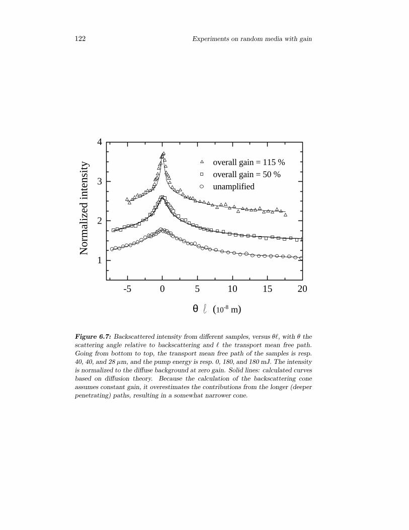
122 Experiments on random media with gain
-5 0 5 10 15 20
1
2
3
4
overall gain = 115 %overall gain = 50 %unamplified
Nor
mal
ized
inte
nsity
θ (10-8 m)
Figure 6.7: Backscattered intensity from different samples, versus θ , with θ the
scattering angle relative to backscattering and the transport mean free path.
Going from bottom to top, the transport mean free path of the samples is resp.
40, 40, and 28 µm, and the pump energy is resp. 0, 180, and 180 mJ. The intensity
is normalized to the diffuse background at zero gain. Solid lines: calculated curves
based on diffusion theory. Because the calculation of the backscattering cone
assumes constant gain, it overestimates the contributions from the longer (deeper
penetrating) paths, resulting in a somewhat narrower cone.
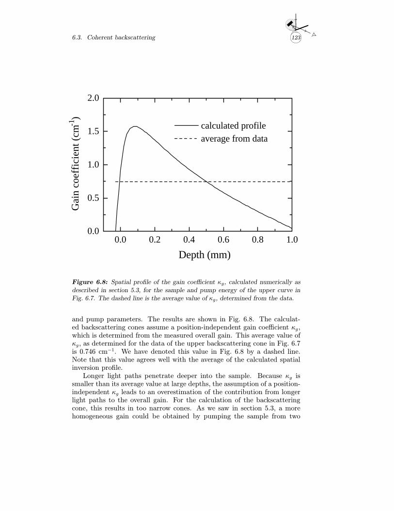
6.3. Coherent backscattering 123
0.0 0.2 0.4 0.6 0.8 1.00.0
0.5
1.0
1.5
2.0
calculated profile average from data
Gai
n co
effi
cien
t (cm
-1)
Depth (mm)
Figure 6.8: Spatial profile of the gain coefficient κg, calculated numerically as
described in section 5.3, for the sample and pump energy of the upper curve in
Fig. 6.7. The dashed line is the average value of κg, determined from the data.
and pump parameters. The results are shown in Fig. 6.8. The calculat-ed backscattering cones assume a position-independent gain coefficient κg,which is determined from the measured overall gain. This average value ofκg, as determined for the data of the upper backscattering cone in Fig. 6.7is 0.746 cm−1. We have denoted this value in Fig. 6.8 by a dashed line.Note that this value agrees well with the average of the calculated spatialinversion profile.
Longer light paths penetrate deeper into the sample. Because κg issmaller than its average value at large depths, the assumption of a position-independent κg leads to an overestimation of the contribution from longerlight paths to the overall gain. For the calculation of the backscatteringcone, this results in too narrow cones. As we saw in section 5.3, a morehomogeneous gain could be obtained by pumping the sample from two
124 Experiments on random media with gain
sides, which leads however to a somewhat smaller average gain.
6.4 Discussion
We have demonstrated the effect of gain on the multiple scattering in-terference phenomenon coherent backscattering. In future experiments, itis interesting to study the combination of amplification with very strongscattering. We saw in chapter 4, that for very strong scattering recurrentscattering becomes important. If gain lengths of the order of the scatteringmean free path could be achieved, the importance of recurrent scatteringcould be enhanced due to gain. If the amplification along a recurrent lightpath is strong enough, this recurrent path could form a ‘random ring cav-ity’ along which laser action could set in. Another interesting experimentwould be, to study the effect of gain on the diffusion constant in a randommedium. If recurrent scattering becomes more important, the diffusionconstant could decrease upon the introduction of gain.
To obtain strong scattering with amplification is difficult from an ex-perimental point of view. A very interesting system would be a randomcollection of mono-disperse titanium dioxide particles (which scatter verystrongly), doped with laser dye. The technological developments on realiz-ing such particles are promising.
125
References and notes
[1] J.F. de Boer, A. Lagendijk, R. Sprik, and S. Feng, Phys. Rev. Lett.71, 3947 (1993).
[2] N.M. Lawandy, R.M. Balachandran, A.S.L. Gomes, and E. Sauvain,Nature 368, 436 (1994).
[3] C. Gouedard, D. Husson, C. Sauteret, F. Auzel, and A. Migus, J. Opt.Soc. Am. B 10, 2358 (1993).
[4] B. Davison and J.B. Sykes, Neutron Transport Theory (Oxford Uni-versity Press, 1958).
[5] Laser Speckle and Related Phenomena, Topics in Applied Physics 9,edited by J.C. Dainty (Springer, Berlin, 1984).
[6] D.J. Pine, D.A. Weitz, P.M. Chaikin, and E. Herbolzheimer, Phys.Rev. Lett. 60, 1134 (1988).
[7] S. Feng, C. Kane, P.A. Lee, and A.D. Stone, Phys. Rev. Lett. 61, 834(1988).
[8] This type of experiment can be used to record the short range angularcorrelation function [9].
[9] J.H. Li and A.Z. Genack, Phys. Rev. E 49, 4530 (1994).[10] Ti:Sapphire crystals were obtained from Single Crystal Technology
B.V. Enschede.[11] M.P. van Albada and A. Lagendijk, Phys. Rev. B 36, 2353 (1987).[12] V.S. Letokhov, Sov. Phys. JETP 26, 835 (1968).[13] H.C. van de Hulst, Multiple Light Scattering (Dover, New York, 1980).[14] M.B. van der Mark, M.P. van Albada, and A. Lagendijk, Phys. Rev.
B 37, 3575 (1988).[15] M.N. Barber and B.W. Ninham, Random and Restricted Walks, (Gor-
don and Breach, New York, 1970).[16] A. Yu. Zyuzin, Europhys. Lett. 26, 517 (1994).[17] Here we assume that the amplification of the measured background
intensity, is completely determined by γ�. This means that we assumethat the single scattering (and stray light) contributions to the back-ground are amplified by the same factor as γ�. If part of these contri-butions is not amplified, κg will be slightly underestimated.

126

Appendix A
List of symbols
Throughout this thesis we use Heaviside-Lorentz units. These are rational-ized Gaussian units and yield elegant an simple equations. (See J.D. Jack-son,Classical Electrodynamics, Appendix on Units and Dimensions (Wiley,New York, 1975).) They also avoid wandering factors of 4π. Both ε0 andµ0 are equal to 1. To convert any equation to SI units, simply replace E(r)by√4πε0E(r) and ε(r) by ε(r)/ε0, with ε0 = 107/4πc20 (A
2s4kg−1m−3).
Notation Explanation Introduction
σs scattering cross section Eq. (1.1)
σt cross section for radiation pressure sec. 1.1.1
σabs absorption cross section sec. 1.1.1
σem emission cross section sec. 5.2.1
σe extinction cross section Eq. (1.2)
s scattering mean free path sec. 1.1.2
transport mean free path Eq. (1.6) abs absorption mean free path Eq. (1.7)
i inelastic mean free path sec. 1.1.2
amp amplification mean free path Eq. (5.1)
g gain mean free path sec. 5.1.1
e extiction mean free path sec. 1.1.2
κ× reciprocal of × sec. 1.1.2
127
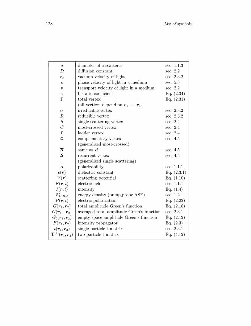
128 List of symbols
a diameter of a scatterer sec. 1.1.3
D diffusion constant sec. 2.2
c0 vacuum velocity of light sec. 2.3.2
c phase velocity of light in a medium sec. 5.3
v transport velocity of light in a medium sec. 2.2γ bistatic coefficient Eq. (2.34)
Γ total vertex Eq. (2.31)
(all vertices depend on r1 . . . r4.)
U irreducible vertex sec. 2.3.2
R reducible vertex sec. 2.3.2
S single scattering vertex sec. 2.4
C most-crossed vertex sec. 2.4
L ladder vertex sec. 2.4
C complementary vertex sec. 4.5(generalized most-crossed)
R same as R sec. 4.5
S recurrent vertex sec. 4.5
(generalized single scattering)
α polarizability sec. 1.1.1
ε(r) dielectric constant Eq. (2.3.1)
V (r) scattering potential Eq. (1.10)
E(r, t) electric field sec. 1.1.1
I(r, t) intensity Eq. (1.4)WG,R,A energy density (pump,probe,ASE) sec. 1.2
P (r, t) electric polarization Eq. (2.22)
G(r1, r2) total amplitude Green’s function Eq. (2.16)
G(r1−r2) averaged total amplitude Green’s function sec. 2.3.1
G0(r1, r2) empty space amplitude Green’s function Eq. (2.12)
F (r1, r2) intensity propagator Eq. (2.3)
t(r1, r2) single particle t-matrix sec. 2.3.1
T(2)(r1, r2) two particle t-matrix Eq. (4.12)
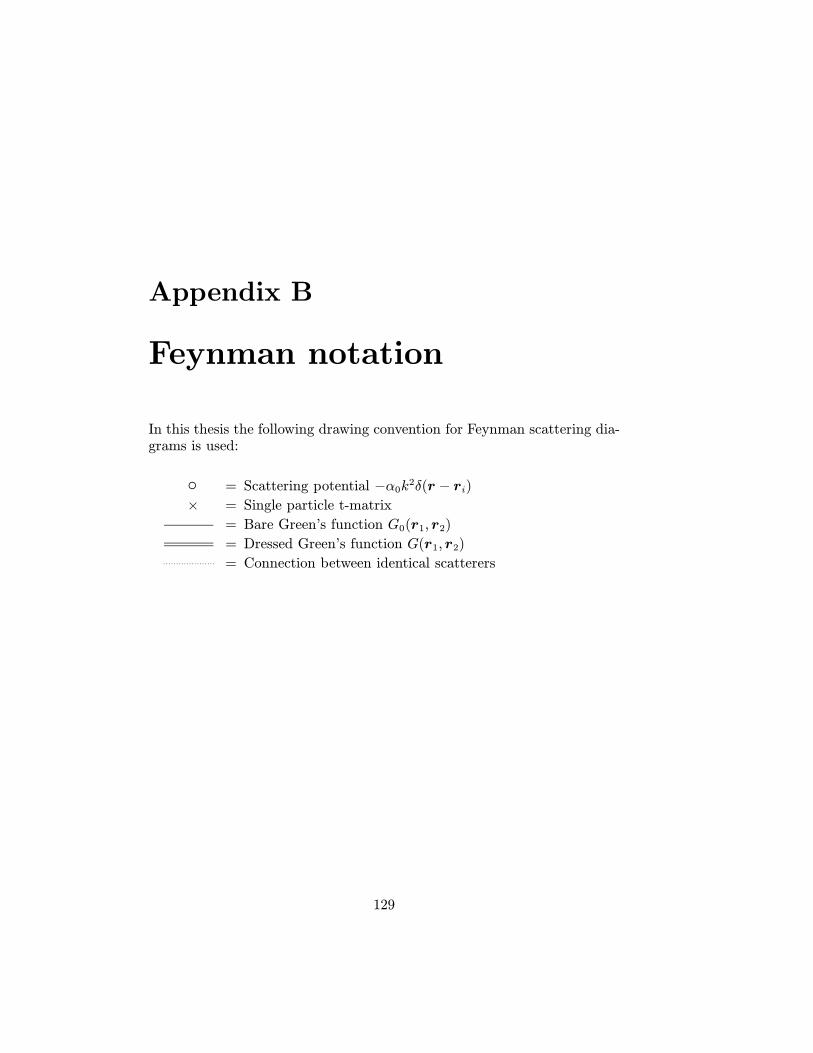
Appendix B
Feynman notation
In this thesis the following drawing convention for Feynman scattering dia-grams is used:
◦ = Scattering potential −α0k2δ(r − ri)
× = Single particle t-matrix
= Bare Green’s function G0(r1, r2)
= Dressed Green’s function G(r1, r2)
= Connection between identical scatterers
129

130
131
Most of the work in this thesis is also published in:
Chapter 3:D.S. Wiersma, M.P. van Albada, and A. Lagendijk, An Accurate Techniqueto Record the Angular Distribution of Backscattered Light, Rev. of Scient.Instr. 66, November issue (1995).
D.S. Wiersma, M.P. van Albada, and A. Lagendijk, in Advances in OpticalImaging and Photon Migration, (Washington, 1994).
D.S. Wiersma, M.P. van Albada, and A. Lagendijk, Precise Weak Local-ization Experiments in Random Structures, in Progress in ElectromagneticResearch (Kluwer, Dordrecht, 1994).
Chapter 4:
D.S. Wiersma, M.P. van Albada, B.A. van Tiggelen, and A. Lagendijk,Experimental Evidence for Recurrent Multiple Scattering Events of Lightin Disordered Media, Phys. Rev. Lett. 74, 4193 (1995).
B.A. van Tiggelen, D.S. Wiersma, and A. Lagendijk, Self-consistent Theoryfor the Enhancement Factor in Coherent Backscattering, Euro Phys. Lett.30, 1 (1995).
Chapter 5:D.S. Wiersma, M.P. van Albada, and A. Lagendijk, Random Laser?,Nature 373, 203 (1995)
D.S. Wiersma and A. Lagendijk, to be submitted to Phys. Rev. E. (1995).
Chapter 6:D.S. Wiersma, M.P. van Albada, and A. Lagendijk, Coherent Backscatter-ing of Light from an Amplifying Random Medium, Phys. Rev. Lett. 75,1739 (1995).

132
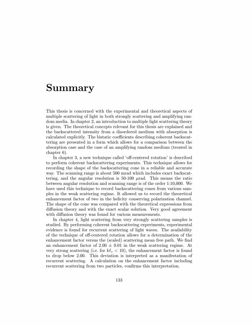
Summary
This thesis is concerned with the experimental and theoretical aspects ofmultiple scattering of light in both strongly scattering and amplifying ran-dom media. In chapter 2, an introduction to multiple light scattering theoryis given. The theoretical concepts relevant for this thesis are explained andthe backscattered intensity from a disordered medium with absorption iscalculated explicitly. The bistatic coefficients describing coherent backscat-tering are presented in a form which allows for a comparison between theabsorption case and the case of an amplifying random medium (treated inchapter 6).
In chapter 3, a new technique called ‘off-centered rotation’ is describedto perform coherent backscattering experiments. This technique allows forrecording the shape of the backscattering cone in a reliable and accurateway. The scanning range is about 500 mrad which includes exact backscat-tering, and the angular resolution is 50-100 µrad. This means the ratiobetween angular resolution and scanning range is of the order 1:10,000. Wehave used this technique to record backscattering cones from various sam-ples in the weak scattering regime. It allowed us to record the theoreticalenhancement factor of two in the helicity conserving polarization channel.The shape of the cone was compared with the theoretical expressions fromdiffusion theory and with the exact scalar solution. Very good agreementwith diffusion theory was found for various measurements.
In chapter 4, light scattering from very strongly scattering samples isstudied. By performing coherent backscattering experiments, experimentalevidence is found for recurrent scattering of light waves. The availabilityof the technique of off-centered rotation allows for a determination of theenhancement factor versus the (scaled) scattering mean free path. We findan enhancement factor of 2.00 ± 0.01 in the weak scattering regime. Atvery strong scattering (i.e. for k s < 10), the enhancement factor is foundto drop below 2.00. This deviation is interpreted as a manifestation ofrecurrent scattering. A calculation on the enhancement factor includingrecurrent scattering from two particles, confirms this interpretation.
133
134 Summary
In chapter 5, amplifying random media are discussed. We go into theexperimental considerations on realizing such media. Different laser materi-als and excitation schemes are discussed and results on powdered ruby andTi:sapphire crystals are given. We find that with powdered Ti:sapphire,amplifying random samples can be realized with transport mean free pathsdown to 20 µm and gain lengths of the order of 10 mm. We examine thetheoretical aspects of amplifying random media by solving numerically theset of diffusion and rate equations describing light propagation in a pow-dered laser crystal. Under certain conditions, the spontaneously emittedlight from such a medium is found to exhibit a pulsed behaviour. Finally,random laser action is discussed.
In chapter 6, experiments are described on amplifying random media.We have recorded laser speckle patterns from pumped Ti:sapphire pow-ders. We find that upon increasing the gain the speckle pattern persistsbut changes. Furthermore, a study on coherent backscattering from anamplifying random medium is presented. We find that the central region ofthe backscattering cone narrows down upon increasing the gain, due to theincreased importance of the longer light paths. The enhancement factorremains unchanged. Also a calculation is performed on coherent backscat-tering from an amplifying random medium in the diffusion approximation.Very good agreement between data and theory is found.
Samenvatting voor iedereen
Dit proefschrift gaat over licht in wanordelijke media. Een voorbeeld vaneen wanordelijk medium is dichte mist. Het licht van bijvoorbeeld de kop-lamp van een auto wordt in dichte mist diffuus: de lichtstralen die door dekoplamp worden uitgezonden worden op een willekeurige manier van richt-ing veranderd door de waterdruppels. Deze richtingsverandering noemenwe verstrooiing. In dichte mist zal het licht vele malen verstrooid worden.Een ander voorbeeld van een wanordelijk medium is witte verf. Witte verfbestaat uit een willekeurige opeenstapeling van kleine korreltjes die, net alswater druppels, het licht verstrooien.
Je kunt je afvragen hoe licht zich voortplant in een wanordelijk mediumzoals mist. Als je op een kleine schaal kijkt, is dit een zeer ingewikkeld pro-bleem: een afzonderlijke lichtstraal wordt vele malen van richting veranderddoor de grote hoeveelheid waterdruppels. Op grote schaal lijkt het probleemechter heel simpel: het licht vormt gewoon een diffuse ‘gloed’. Er is echtermeer aan de hand. Omdat licht zich gedraagt als een golf kan er namelijkinterferentie optreden. Wat is interferentie ?
Interferentie is een effect dat kan optreden voor elk soort golf, zoalslicht, geluid, radiogolven of golven in het water, en ontstaat als twee ofmeer golven bij elkaar komen. Als er in een concertzaal (met een te drogeakoestiek) op twee fluiten precies dezelfde toon gespeeld wordt, dan hangtwat je hoort af van waar je zit in de zaal. Hoe de geluidsgolven van de tweefluiten optellen, hangt namelijk af van hun onderlinge ‘fase’. Als de beidegolven net dezelfde beweging maken als ze elkaar tegen komen, werkenze samen en ontstaat er een sterkere beweging. De golven zijn dan ‘infase’ en de interferentie is constructief. Het totale geluid dat je dan hoortis heel hard. Als ze daarentegen net een tegengestelde beweging makenheffen ze elkaar op. Ze zijn dan ‘uit fase’ met elkaar en de interferentie heetdestructief. Je hoort in dat geval helemaal niets. Als je door de concertzaalloopt, kom je afwisselend op plaatsen waar de golven constructief optellenen waar ze elkaar uitdoven, en je hoort het geluid dus harder en zachterworden.
135
136 Samenvatting
Interferentie kan ook optreden voor lichtgolven. Stel, we nemen eenscherm met twee nauwe spleten erin, en belichten dat aan de achterkantmet een zaklamp. De spleten zijn vergelijkbaar met de fluiten in het boven-staande voorbeeld voor geluidsgolven. Beide spleten zullen aan de voorkantvan het scherm lichtgolven uitzenden. Net als bij de fluiten zal op verschil-lende plaatsen het licht constructief of destructief interfereren. Als je hetlicht dat van de twee spleten afkomt op een wit stuk papier laat vallen, zieje lichte en donkere lijnen, corresponderend met de plaatsen waar de licht-golven respectievelijk constructief optellen of elkaar opheffen. Bovendien,als je de spleten verder van elkaar brengt komen de lichte en donkere lijnendichter bij elkaar en omgekeerd. Dit is een beroemd experiment dat voorhet eerst uitgevoerd is door Thomas Young (1773–1829).
Interferentie van licht treedt ook op als het licht verstrooid wordt in bij-voorbeeld mist of witte verf. Een belangrijk voorbeeld daarvan is ‘coherenteterugverstrooiing’. Als we met bijvoorbeeld een halogeen spotje van een af-stand schijnen op een wit geverfde muur, dan zal de witte verf het licht inalle richtingen verstrooien: vanaf iedere plaats in de kamer zie je een lichteplek op de muur. Als je echter precies op de plaats van het spotje zou kun-nen gaan staan, zou je iets bijzonders zien. Voor het licht dat van de muurterug naar het halogeen spotje wordt verstrooid, treedt er namelijk con-structieve interferentie op. In de richting terug naar het spotje (genoemdde ‘terugstrooirichting’), wordt er meer licht verstrooid dan in alle andererichtingen. Waar komt dit effect vandaan ?
Laten we eens twee punten beschouwen in het belichte oppervlak vande verf. Er is licht dat op het ene punt invalt, en na een wanordelijkewandeling door de verf vanaf het andere punt weer naar buiten komt. Eris echter ook licht dat precies het omgekeerde doet. Als het licht in beidegevallen hetzelfde pad afgelegd heeft, is het als het naar buiten komt nogsteeds in fase. De twee punten op het oppervlak kan je dan vergelijken metde twee spleten in het experiment van Young. Het licht dat van deze tweepunten afkomt zal ook lichte en donkere strepen geven. Ieder stel puntenin het belichte oppervlak van de verf geeft een dergelijk streeppatroon.Het totale verstrooide licht is dus de som van een heleboel streeppatronen,die varieren van heel fijn tot heel grof. Net als in het experiment vanYoung, wordt de afstand tussen de strepen in een patroon bepaald doorde afstand tussen de twee punten in het belichte oppervlak, en de afstandtussen die twee punten hangt natuurlijk weer samen met de weg die hetlicht door het medium heeft gevolgd. Alle streeppatronen hebben echtereen ding gemeen: in de richting terug naar het halogeen spotje vind jealtijd een lichte streep. Daarom is de hoeveelheid licht die in die richtingwordt verstrooid groter dan de hoeveelheid licht in andere richtingen. Om
137
coherente terugverstrooiing waar te nemen is lastig, omdat je de verstrooidehoeveelheid licht wilt meten op de plaats van de lichtbron (het spotje) endicht daaromheen. Hoe je dat toch nauwkeurig kunt doen is beschreven inhoofdstuk 3.
Laten we het eens zwart-wit zien. Als licht op een voorwerp valt, kanhet behalve verstrooid ook geabsorbeerd worden. Als al het licht geab-sorbeerd wordt, is een voorwerp zwart. Als het gedeeltelijk geabsorbeerden gedeeltelijk verstrooid wordt, dan is een voorwerp grijs. Als er helemaalgeen absorptie optreedt, dan is een voorwerp perfect wit. In het dagelijksleven echter absorberen alle voorwerpen tenminste een klein beetje.
In dit proefschrift worden twee soorten wanordelijke media onderzocht.Het eerste is een medium dat verstrooit en waarin het omgekeerde vanabsorptie plaatsvindt: versterking. Wat gebeurt er als de hoeveelheidlicht meer in plaats van minder wordt bij verstrooiing aan een voorwerp?Het voorwerp is dan pas echt wat men altijd met wasmiddelen claimt tebereiken: witter dan wit! In het eerste deel van hoofdstuk 5 wordt uitvoerigingegaan op het maken van een dergelijk medium. Ik gebruik daartoe eenkristal van het materiaal titaan-saffier dat ook gebruikt wordt voor eenlaser. Dergelijke kristallen zijn in staat om licht te versterken, hetgeen ookhet principe is waar een laser op berust. Om dit kristal licht te laten ver-sterken moet het eerst ‘opgeladen’ worden met een sterke lichtpuls. Als erdaarna een tweede (zwakkere) puls op het verpoederde kristal valt, zal dezetweede puls zowel verstrooid als versterkt worden. Nadat het mogelijk wasom een versterkend wanordelijk medium te maken, ben ik experimenten metdergelijke media gaan doen, waaronder metingen aan coherente terugver-strooiing. Deze metingen met de bijbehorende theorie staan beschreven inhoofdstuk 6.
Om meer inzicht te krijgen in het gedrag van versterkende wanordelijkemedia, heb ik numerieke berekeningen aan een dergelijk medium gedaan.Het is bijvoorbeeld interessant om te kijken wat er gebeurt als er in hetopgeladen medium zoveel versterking plaatsvindt dat er per seconde meerlicht ontstaat dan dat er weg kan stromen. Dan wordt de hoeveelheidlicht zeer snel erg groot. Deze situatie kan echter niet onbeperkt blijvenbestaan, en als het medium ‘leeg’ is neemt de hoeveelheid licht weer snelaf. Dit proces kan zich een aantal malen herhalen als het medium steedsweer opnieuw opgeladen wordt, en het resultaat is dat het medium gepulstlicht uitzendt. Dit staat beschreven in hoofdstuk 5. Aan het einde van dathoofdstuk wordt ook besproken in hoeverre dit systeem gezien kan wordenals een ‘wanordelijke laser’.
Behalve versterkende media heb ik ook zeer sterk verstrooiende mediabestudeerd. Een sterk verstrooiend medium is een medium waarin een licht-
138 Samenvatting
straal zeer vaak achter elkaar verstrooid wordt. De lichtstraal kan zich dussteeds maar over zeer kleine afstanden vrij voortplanten voordat hij alweervan richting wordt veranderd. Die afstand waarover een lichtstraal zichgemiddeld vrij kan voortplanten in een medium, wordt de ‘verstrooiings-vrijeweglengte’ genoemd. De verstrooiings-vrijeweglengte geeft dus de mateaan waarin een medium verstrooit. Merk op dat een kleine verstrooiings-vrijeweglengte een grote mate van verstrooiing betekent.
Als nu een medium zo sterk verstrooit dat de verstrooiings-vrijeweglengte van dezelfde orde van grootte wordt als de golflengte vanhet licht, ontstaat er een vreemde situatie. Een lichtgolf kan zich danniet eens meer vrij voortplanten over de afstand van een golflengte. In dezesituatie zou er wat genoemd wordt ‘Anderson lokalisatie’ op kunnen treden.Dit is een interferentie-effect waarnaar al een tijd gezocht wordt. Door dezeer sterke verstrooiing zou al het licht langs gesloten paden (‘lussen’) gaanlopen en daarmee in het medium opgesloten (gelokaliseerd) zijn. Doorcoherente terugverstrooiing van een sterk verstrooiend medium te bestu-deren, hebben we experimenteel bewijs gevonden dat er licht langs geslotenpaden kan gaan lopen. Dit wordt beschreven in hoofdstuk 4.
Wat in de nabije toekomst interessant kan zijn, is de combinatie van zeersterke verstrooiing met versterking. Ten gevolge van versterking wordenlange paden in een medium belangrijker: hoe langer een pad, hoe groterde totale versterking langs het pad is. Door zeer sterke verstrooiing enversterking te combineren zou het effect van de gesloten paden misschienzo belangrijk kunnen worden dat Anderson lokalisatie van licht optreedt.
Dankwoord
Allereerst wil ik mijn promotor Ad Lagendijk heel hartelijk bedanken omdathij me aan de ene kant een enorme vrijheid en vertrouwen gegeven heeft ommijn eigen weg te gaan, en aan de andere kant me daarbij altijd gesteundheeft als ik daarom vroeg. Om verder te komen in het onderzoek was allesmogelijk. Toen ik je om middernacht probeerde te bereiken omdat ik ietsleuks gemeten had, belde je me 10 min. later vol interesse vanuit Parijsterug terwijl je volgens mij nog niet eens je jas uit had. Jouw enthousiasmevoor de natuurkunde vind ik heel inspirerend. Een van de dingen die ikvan je geleerd heb tijdens de vele uren waarin je met mij en Marco eenaantal boeken hebt doorgenomen, is op welke mooie manier veel zaken inde natuurkunde samenhangen.
Ook mijn co-promotor Meint van Albada wil ik hartelijk bedanken. Ikheb veel geleerd van jouw kijk op een experiment waarbij je altijd de kernvan de zaak naar boven wist te halen. Je vasthoudendheid en enthousias-me om problemen volledig te doorgronden heb ik altijd erg gewaardeerd.Verder sprak jouw werkwijze waarbij niet de glans maar wel de func-tionaliteit van de apparatuur de doorslaggevende factor tot aanschaf wasmij erg aan. Ons uitstapje om een YAG-laser uit Orsay te halen vond ikdan ook heel leuk.
Erik-Jan Kossen wil ik bedanken voor alle technische steun. Je wasaltijd zeer betrokken bij de experimenten en bereid om snel problemen aante pakken. Toen de voeding van de Argon laser was ontploft hebben wesamen nog de hele avond transistors zitten solderen. Nogmaals bedanktdaarvoor.
Ook Rob Kemper wil ik bedanken voor zijn technische steun. Als ikweer eens een raar component zocht, wist jij altijd wel ergens een laatje tevinden waarvan iedereen verder al lang vergeten was dat er het betreffendeonderdeel in lag.
139
140 Dankwoord
Daan Frenkel wil ik bedanken voor het gebruik van de computers inzijn groep en voor het niet boos worden toen er een ‘automatische werker’een hele ochtend zijn bureau ingepikt had. Je inspirerende lezingen warenverder altijd voor mij het hoogtepunt van de colloquium cyclus op Amolf.
I would like to thank Thiery Lehoux and Yves Potiron of Quantel Francein Paris, who helped me out when one of my YAG-rods had a burn. Youstayed on a free afternoon, so I could come by with the laser oscillatorbefore the holiday started.
Mijn moeder wil ik bedanken omdat ze me altijd gestimuleerd heeft omte gaan studeren en me daarbij ook steeds gesteund heeft. Wat het thuisvroeger ook erg leuk maakte was dat alles kon dat je creatief of leerzaamvond. De opgedane handigheid van alle hobbies is nu bij het experimenterengoed van pas gekomen.
Maarten Hagen wil ik bedanken voor het gebruik van zijn computerom de videocamera in mijn opstelling uit te lezen. Je hebt me ook goedgeholpen bij het schrijven van de juiste acquisitie programma’s.
Bart van Tiggelen wil ik bedanken voor de mooie berekeningen aan‘recurrent scattering’ en voor alle discussies die we daarover hebben ge-voerd. Ook bedankt voor de constructieve kritiek die je gegeven hebt ophet theoretische gedeelte van hoofdstuk 4.
Bart Noordam heeft me goed geholpen met het bouwen van een gepul-ste dye laser. Ook bedankt voor het lenen van de juiste optica daarvoor.Verder wil ik Anton Buyzerd en Raluca Constantinescu bedanken voor hunTi:saffier laserstaaf die ik mocht verpulveren.
Het Amolf is een inspirerende omgeving waar veel samengewerkt wordt,en iedereen altijd bereid is je te helpen of vragen te beantwoorden. Ikwil een aantal mensen met wie ik veel te maken heb gehad expliciet be-danken, namelijk: David van Coevoorden, Adriaan Tip, Rob Uiterlinden,Frans Vitalis, Saskia Windhouwer, Wim van der Zande, Piet Kea, HuibBakker, Els Ruscaa-Steunebrink, Ilja Stavenuiter, Raluca Constantinescu,Trees zur Kleinsmiede-van Dongen, Marianne ter Stroot-Schouw, MaartenHagen, Willem-Jan Huisman, Henk Dekker, Idsard Attema, Mischa Bonn,Marc-Paul de Boer, Klaas-Jan van Druten, Marcel Lankhuyzen, Ben v.d.Linden v.d. Heuvell, Harm Geert Muller, Rutger Vrijen, Eloy Wouters, enMark Brongersma. De mensen van de groep van Jaap Boon wil ik verderbedanken voor het gebruik van het chemisch laboratorium, en hun assis-tentie bij het bereiden van mijn samples.
141
I wish to thank Lucia Mariotto for her loving care during the writing ofpart of my thesis in Verona. Your creative, enthusiastic, and curious wayof living your life, is very inspiring. La tua presenza nella mia vita heefteen grote waarde voor mij.
Bart Broers wil ik bedanken voor alle gedreven discussies zowel overnatuurkunde als over bijvoorbeeld biedsystemen. Jouw scherpe blik wistvaak de essentie van een probleem te raken. Ik heb bovendien erg genotenvan de zomerschool met jou op Kreta, waar we bijna de hele natuurkundegevat hebben in gitaarsnaren.
Edwin Brouwer van de firma Melles Griot wil ik bedanken voor hetbelangstellende meedenken met onze experimenten. Als ik weer eens iets‘eigenlijk de volgende dag nodig had’, wist je altijd wel een manier te vindenom dat voor elkaar te krijgen.
John en Jaqueline wil ik bedanken voor alle vegetarische sates-meerhoekmet rijst en een gekookt eitje. Het was heel fijn om af en toe bij jullie even‘op te laden’.
De UvA-groep was voor mij altijd een goede plek voor om met mensente discussieren over lichtverstrooiing en aanverwante zaken. Rik, Johannes,Mischa, Mark, Mark, Peter, Rudolf en Willem Bos, bedankt voor jullieenthousiasme en hulp. Mischa wil ik verder bedanken voor de samenwerkingbij het zoeken naar diffusieconstantes met versterking.
Marina wil ik, ditmaal niet op haar eigen verzoek, heel erg bedankenvoor met name alles. Op een indirecte manier heb je meer aan dit boekjebijgedragen dan je misschien zelf zou denken.
Christiaan Alofs wil ik bedanken voor zijn steun met name tijdens delaatste fase van het schrijven van mijn proefschrift. Je hulp als paranimf bijhet regelen van alle zaken rondom mijn (en Marco’s) promotie heb ik zeergewaardeerd. Verder heb ik veel gehad aan je kritisch en helder commentaarop de een na laatste versie van mijn proefschrift.
Vorrei ringraziare Sandro Etalle per avermi convinto che fare parapen-dio di Domenica e molto bello. Molte grazie anche per avermi supportatoin entrambe i nostri mondi.
Ondanks dat Bas Bijvoet bedankt wil worden voor verder helemaalniets, wil ik hem bedanken voor ondermeer het feit dat, ondanks zijn nietaflatende enthousiasme tijdens het experimenteren om de gehele opstellente verbouwen, ik niet de optische tafel een kwart slag gedraaid terugvondbij terugkeer uit Italie, en desalniettemin hij daar leuke meetingen mee hadgedaan en deed. Ook bedankt voor het kritisch lezen van en zeer bruikbaarcommentaar leveren op mijn proefschrift.
Marco, zonder jou had mijn promotietijd er heel anders uitgezien. Ze
142 Dankwoord
zeggen dat je niet met je echtgenoot(e) moet samenwerken, maar met jouging dat juist erg goed. We vulden elkaar fantastisch aan, en hadden daarallebei ook erg veel plezier in. Wat ik zo mooi daaraan vond was, datwe onze onderlinge verschillen juist gebruikten om elkaar verder te helpen.Daarom heb ik ook veel van je geleerd. Ondanks dat we geen experimentsamen uitgevoerd hebben omdat we twee verschillende projecten deden,heb ik toch het gevoel dat ik alles met jou samen heb gedaan. Ik hebeen fantastische tijd met je gehad de afgelopen vier jaar, zowel binnen alsbuiten het lab. Ik hoop dat we straks ondanks 1500 km, ons huwelijk tochop een bepaalde manier voort kunnen zetten.

143

Druk: drukkerij Sigma B.V.Lithografie: R & H grafipartners