Lifelong Multi-Agent Path Finding in Large-Scale Warehouses

Jiaoyang Li1 , Andrew Tinka2 , Scott Kiesel2 , Joseph W. Durham2 ,T. K. Satish Kumar1 and Sven Koenig1

1University of Southern California2Amazon Robotics

jiaoyanl@usc.edu, {atinka, skkiesel, josepdur}@amazon.com, tkskwork@gmail.com, skoenig@usc.edu

AbstractMulti-Agent Path Finding (MAPF) is the problemof moving a team of agents to their goal locationswithout collisions. In this paper, we study the life-long variant of MAPF where agents are constantlyengaged with new goal locations, such as in large-scale warehouses. We propose a new frameworkfor solving lifelong MAPF by decomposing theproblem into a sequence of Windowed MAPF in-stances, where a Windowed MAPF solver resolvescollisions among the paths of the agents only withina finite time horizon and ignores collisions beyondit. Our framework is particularly well suited to gen-erating pliable plans that adapt to continually arriv-ing new goal locations. Theoretically, we analyzethe advantages and disadvantages of our frame-work. Empirically, we evaluate our framework witha variety of MAPF solvers and show that it can pro-duce high-quality solutions for up to 1,000 agents,significantly outperforming existing methods.

1 IntroductionMulti-Agent Path Finding (MAPF) is the problem of movinga team of agents on a graph from their start locations to theirgoal locations while avoiding collisions. The quality of a so-lution is measured by flowtime (the sum of the arrival timesof all agents at their goal locations) or makespan (the maxi-mum of the arrival times of all agents at their goal locations).MAPF is NP-hard to solve optimally [Yu and LaValle, 2013].

MAPF has numerous real-world applications, such as au-tonomous aircraft-towing vehicles [Morris et al., 2016], of-fice robots [Veloso et al., 2015], video game characters [Maet al., 2017b], and quadrotor swarms [Honig et al., 2018].Today, in autonomous warehouses, mobile robots called driveunits already autonomously move inventory pods or flat pack-ages from one location to another [Wurman et al., 2007;Kou et al., 2020]. However, MAPF is only the “one-shot”variant of the actual problem in many real-world applications.Typically, after an agent reaches its goal location, it does notstop and wait there forever. Instead, it is assigned a new goallocation and required to keep moving, which is referred to aslifelong MAPF [Ma et al., 2017a] and characterized by agentsconstantly being assigned new goal locations.

Existing methods for solving lifelong MAPF include (1)solving it as a whole [Nguyen et al., 2017], (2) decomposingit into a sequence of MAPF instances where one replans pathsat every timestep for all agents [Wan et al., 2018; Grenouil-leau et al., 2019], and (3) decomposing it into a sequence ofMAPF instances where one plans new paths at every timestepfor only the agents with new goal locations [Cap et al., 2015;Ma et al., 2017a; Liu et al., 2019].

In this paper, we propose a new framework for solving life-long MAPF where we decompose lifelong MAPF into a se-quence of Windowed MAPF instances and replan paths onceevery h timesteps (h is user-specified) for interleaving plan-ning and execution. A Windowed MAPF instance is differentfrom a regular MAPF instance in the following ways: (1) itallows an agent to be assigned a sequence of goal locationswithin the same planning horizon, and (2) collisions need tobe resolved only for the first w timesteps (w ≥ h is user-specified). The benefit of this decomposition is two-fold.First, it keeps the agents continually engaged, avoiding idletime, and increasing throughput. Second, it generates pliableplans that adapt to continually arriving new goal locations. Infact, resolving all collisions within the entire time horizon isoften unnecessary since the paths of the agents can change asnew goal locations arrive.

We evaluate our framework with various MAPF solvers,namely, CA* [Silver, 2005] (incomplete and subopti-mal), PBS [Ma et al., 2019] (incomplete and suboptimal),ECBS [Barer et al., 2014] (complete and bounded subopti-mal) and CBS [Sharon et al., 2015] (complete and optimal).We show that, for each MAPF solver, using a bounded hori-zon yields similar throughput as using the full horizon butwith significantly smaller runtime. We also show that ourframework outperforms existing work and can scale up to1,000 agents.

2 BackgroundIn this section, we first introduce several state-of-the-art

MAPF solvers, and we then discuss several existing researchon lifelong MAPF. We finally review the elements of thebounded horizon idea that have guided previous research.

2.1 Popular MAPF SolversCBS Conflict-Based Search (CBS) [Sharon et al., 2015] is apopular two-level MAPF solver that is complete and optimal.

arX

iv:2

005.

0737

1v1

[cs

.AI]

15

May

202

0

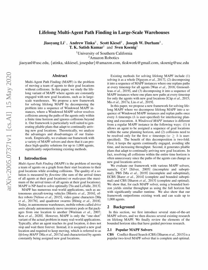
(a) Fulfillment warehouse map, borrowed from [Wurman etal., 2007].

(b) Sorting center map, reproduced from [Wan et al., 2018].

Figure 1: A well-formed fulfillment warehouse map and a non-well-formed sorting center map. In (a), the endpoints consist of greencells (representing locations that store inventory pods) and blue cells(representing the packing stations). In (b), the endpoints consistof blue cells (representing locations where the drive units drop offpackages) and pink cells (representing the loading stations). Blackcells labeled “X” represent chutes (obstacles).

At the high level, CBS starts with a root node which containsa shortest path for each agent (ignoring other agents). It thenchecks for collisions. It chooses and resolves a collision bygenerating two child nodes, each with an additional constraintthat prohibits one of the agents involved in the collision frombeing at the colliding location at the colliding timestep. Itthen calls its low level to replan the paths of the agents withnew constraints. CBS repeats this procedure until finding anode with collision-free paths.

ECBS Enhanced CBS (ECBS) [Barer et al., 2014] is a com-plete and bounded-suboptimal variant of CBS. The boundedsuboptimality (that is, the solution cost is within a user-specified factor times the optimal solution cost) is achievedby using focal search [Pearl and Kim, 1982], instead of best-first search, in both the high- and low-level searches of CBS.

CA* Cooperative A* (CA*) [Silver, 2005] is based on asimple prioritized-planning scheme: Each agent is given aunique priority and computes, in priority order, a shortestpath that does not collide with the (already planned) pathsof agents with higher priorities. CA*, or in general, priori-tized planning, is well known for its small runtime. However,it is incomplete and suboptimal.

PBS Priority-Based Search (PBS) [Ma et al., 2019] com-bines the ideas of CBS and CA*. The high level of PBS issimilar to CBS except that the constraint it adds to each childnode is that one of the agents involved in the collision hashigher priority than the other agent. The low level of PBS issimilar to CA* where it plans a shortest path that is consistentwith the partial priority ordering generated by the high level.It outperforms many variants of prioritized planning solversbut is still incomplete and suboptimal.

2.2 Prior Work on Lifelong MAPFMethod (1) Nguyen et al. [2017] solves lifelong MAPF asa whole in an offline setting and formulates it as an answer setprogramming problem. However, in their paper, the methodonly scales up to 20 agents, each with only about 4 goal lo-cations. This is not surprising because MAPF itself is a chal-lenging problem and its lifelong variant is even harder.Method (2) A second method is to decompose lifelongMAPF into a sequence of MAPF instances where one replanspaths at every timestep for all agents. To improve the scal-ability, researchers have developed incremental search tech-niques to reuse search efforts. For example, Wan et al. [2018]proposes an incremental CBS which reuses the high-level treeof the previous search. However, it has substantial overheadin constructing a new high-level tree from the previous oneand thus does not improve the scalability by much. Svan-cara et al. [2019] uses the framework of Independence De-tection [Standley, 2010] to reuse the paths from the previousiteration. It replans paths for only the new agents (in our case,agents with new goal locations) and the agents whose pathsare affected by the paths of the new agents. However, whenthe environment is dense (that is, many agents with many ob-stacles), almost all paths are affected, and thus it still needs toreplan paths for all agents.Method (3) A third method is similar to the second method,but restricts the replanning to planning paths for only theagents that have just reached their goal locations. The newpaths need to avoid collisions not only with each other butalso with the paths of other agents. Hence, this method coulddegenerate to prioritized planning in the case where only oneagent reaches its goal location at every timestep. As a re-sult, the general drawbacks of prioritized planning, namelyits incompleteness and its potential to generate costly solu-tions, resurface in this method. To address the incomplete-ness issue, Cap et al. [2015] introduces the idea of the well-formed infrastructure to enable backtrack-free search. In awell-formed infrastructure, all possible goal locations are re-garded as endpoints, and, for every pair of endpoints, thereexists a path that connects them without traversing any otherendpoints. In real-world applications, some maps, such asFigure 1(a), may satisfy this well-formed requirement, butsome other maps, such as Figure 1(b), may not. Moreover,additional mechanisms during path planning are required. Forexample, one needs to force the agents to “hold” their goallocations [Ma et al., 2017a] or plan “dummy paths” for theagents [Liu et al., 2019] after they reach their goal locations.Both alternatives cause unnecessarily longer paths for agents,decreasing the overall throughput, as shown in our experi-ments.Summary Method (1) needs to know all goal locations apriori and has limited scalability. Method (2) can work foran online setting and scales better than Method (1). However,replanning for all agents at every timestep is time-consumingeven if one uses incremental search techniques. As a result,its scalability is also limited. Method (3) scales to substan-tially more agents than the first two methods but both themap and the MAPF model need to have additional structureto guarantee the completeness. As a result, it works only

for specific classes of lifelong MAPF instances. In addition,Methods (2) and (3) plan at every timestep, which may not bepractical since planning is time-consuming.

2.3 Bounded-Horizon PlaningBounded-horizon planning is not a new idea. Silver [2005]has already applied this idea to solve regular MAPF withCA*. He refers to it as WHCA* and empirically shows that,as the length of the horizon decreases, WHCA* runs fasterbut also generates longer paths. In this paper, we showcasethe benefits of applying this idea to lifelong MAPF and toother types of MAPF solvers. In particular, our frameworkyields the benefits of lower computational costs for planningwith bounded horizons, while continually keeping the agentsbusy, and yet making only a negligible compromise on thesolution qualities. When executing lifelong MAPF plans ondrive units, Honig et al. [2019] uses a similar framework in-terleaving planning and execution. In such domains, our newframework can be incorporated to interleave planning and ex-ecution more effectively. Such interleaving is even used invideo games [Sigurdson et al., 2018].

3 Problem DefinitionThe input is a graph G = (V,E), whose vertices V corre-spond to locations and whose edges E correspond to con-nections between two neighboring locations, and a set of magents {a1, . . . , am}, each with an initial location. We are in-terested in an online setting where we do not know all goal lo-cations a priori. We assume that there is a task assigner (out-side of our path-planning system) that the agents can requestgoal locations from during the operation of the system. Timeis discretized into timesteps. At each timestep, every agentcan either move to a neighboring location or wait at its currentlocation. Both move and wait actions have unit duration. Acollision occurs iff two agents plan to occupy the same loca-tion at the same timestep (called a vertex conflict in [Stern etal., 2019]) or to traverse the same edge in opposite directionsat the same timestep (called a swapping conflict in [Stern etal., 2019]). Our task is to plan collision-free paths that moveall agents to their goal locations and maximize the through-put, that is, the average number of goal locations visited pertimestep.

The task assignment is usually domain-dependent andcould have constraints and preferences of its own in dif-ferent domains. Therefore, we study the general case inwhich the task assigner is not necessarily within our con-trol so that our path-planning system is applicable in manydifferent domains. But, of course, for a particular domain,we can design a hierarchical framework that combines adomain-specific task assigner with our path-planning sys-tem. For example, the task assigners in [Ma et al., 2017a;Liu et al., 2019] for fulfillment warehouse applications andin [Grenouilleau et al., 2019] for sorting center applicationscan be directly combined with our path-planning system. Wealso showcase two simple task assigners in our experiments.Moreover, the hierarchical framework is also usually a goodway to achieve efficiency and improve scalability.

4 FrameworkOur framework has two user-specified parameters, namely,the time horizon w and the replanning frequency h. The timehorizon w specifies that the Windowed MAPF solver has toresolve collisions within a time horizon of w timesteps. Thereplanning frequency h specifies that the Windowed MAPFsolver has to replan paths once every h timesteps. To executesuccessfully, the Windowed MAPF solver has to replan pathsmore frequently than once every w timesteps, i.e., w shouldbe larger than or equal to h.

In every Windowed MAPF episode, say, starting attimestep t, we first update the start location si and the goallocation sequence gi for each agent ai. We set the start lo-cation si of agent ai to its location at timestep t. Then, wecalculate the minimum number of steps d that agent ai needsto visit all remaining locations in gi, i.e.,

d = dist(x ,gi[0]) +

|gi|−1∑j=1

dist(gi[j − 1],gi[j]),

where dist(x, y) is the distance between locations x and y and|x| is the cardinality of set x. d being smaller than h indicatesthat agent ai might finish visiting all its goal locations andbeing idle before the next planning episode starts at timestept+h. To avoid this situation, we continually assign new goallocations to agent ai until d ≥ h. Once the start locations andthe goal location sequences for all agents require no more up-dates, we call a Windowed MAPF solver to find paths for allagents that are collision-free for the first w timesteps and thatmove them from their start locations through all their goal lo-cations in the order given by their goal location sequences.Finally, we move the agents for h timesteps along the gener-ated paths and remove the visited goal locations from the goallocation sequences.

We use flowtime as the objective of the Windowed MAPFsolver, which is known to be a reasonable objective for life-long MAPF [Svancara et al., 2019]. Compared to regu-lar MAPF solvers, the Windowed MAPF solvers need to bechanged in two aspects: (1) each path needs to go througha sequence of goal locations, and (2) any two paths need tobe collision-free for only the first w timesteps. We describethese changes in detail in the following two subsections.

4.1 A* for a Sequence of Goal LocationsAll the MAPF solvers discussed in Section 2.1 use state-timeA* [Silver, 2005] or any of its variants in their low-levelsearches to find a path for each agent from its start location toits unique goal location while satisfying some given spatio-temporal constraints that prohibit the agent from being at cer-tain locations at certain timesteps. However, a characteristicfeature of a Windowed MAPF solver is that, for each agent,it plans a path that goes through a sequence of goal locations.In fact, Grenouilleau et al. [2019] performs a truncated ver-sion of this adaptation in the study of the pickup and deliveryproblem. They propose Multi-Label A* that can find a pathfor a single agent that goes through two ordered goal loca-tions, namely its assigned pick up location and goal location.In Algorithm 1, we generalize Multi-Label A* to a sequenceof goal locations.

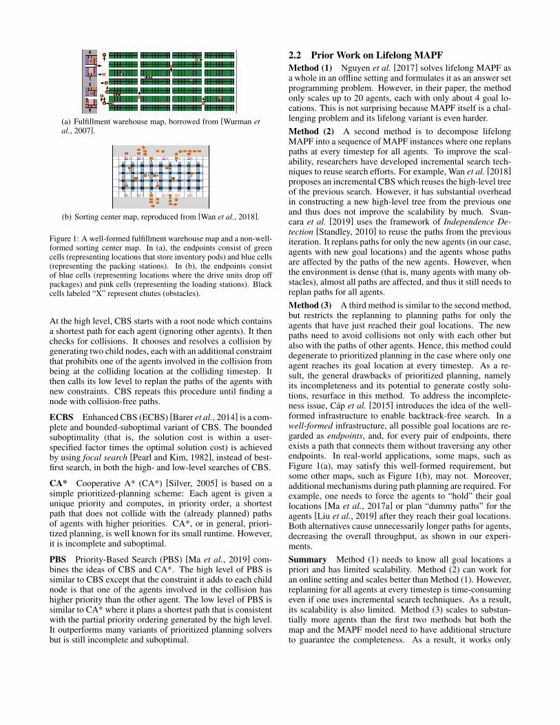
Algorithm 1: The low-level search for Windowed MAPFsolvers. The difference from state-time A* is shown in blue.

Input: Start location si, goal location sequence gi.

1 R.location ← si, R.time ← 0, R.label ← 0, R.g ← 0;2 R.h← COMPUTEHVALUE(R.location , R.label );3 open .push(R);4 while open is not empty do5 P ← open .pop(); // Pop the node with the minimum f .6 if P.location = gi[P.label ] then // Update label.7 P.label ← P.label + 1;

8 if P.label = |gi| then // Goal test.9 return the path retrieved from P ;

10 foreach child node Q of P do // Generate child nodes.11 open .push(Q);

12 return “No Solution”;

13 Function COMPUTEHVALUE(Location x, Label l) :14 return dist(x ,gi[l ]) +

∑|gi|−1j=l+1 dist(gi[j − 1],gi[j]);

Algorithm 1 uses the structure of state-time A*. For eachnode N , we add an additional attribute N.label that indicatesthe number of goal locations in the goal location sequence gi

that the corresponding path from the root node to node N hasalready visited. For example, N.label = 2 indicates that thecorresponding path has visited goal locations gi[0] and gi[1]but not goal location gi[2]. Algorithm 1 computes the h-valueof a node as the distance from the location of the node to thenext goal location plus the sum of the distances between con-secutive future goal locations in the goal location sequence[Lines 13-14]. In the main procedure, Algorithm 1 first cre-ates the root node R with a label of 0 and pushes it into theprioritized queue open [Lines 1-2]. While open is nonempty[Line 4], the node P with the smallest f -value is selected forexpansion [Line 5]. If P has reached its current goal loca-tion [Line 6], P.label is increased by 1 [Line 7]. If P.labelequals the cardinality of the goal location sequence [Line 8],Algorithm 1 terminates and returns the corresponding path[Line 9]. Otherwise, it generates child nodes that respect thegiven spatio-temporal constraints [Lines 10-11]. The labelsof the child nodes equal P.label . Checking for duplicates inopen requires a comparison of labels in addition to other at-tributes.

4.2 Bounded-Horizon MAPF SolversAnother characteristic feature of Windowed MAPF solvers isthe use of a bounded horizon. Regular MAPF solvers canbe easily adapted to resolve collisions for only the first wtimesteps. Beyond the first w timesteps, the solvers ignorecollisions between agents and assume that each agent followsits individual shortest path to go through all its goal locations,which ensures that the agents still head in the correct direc-tions. Modification details of the various MAPF solvers dis-cussed in Section 2.1 are as follows.

Bounded-Horizon (E)CBS Both CBS and ECBS con-duct search by detecting and resolving collisions. In theirbounded-horizon variants, we only need to modify the col-lision detection function. While (E)CBS finds collisions

among all paths and resolves any existing ones, bounded-horizon (E)CBS only finds collisions among all paths thatoccur in the first w timesteps and resolves any such exist-ing ones. The remaining parts of (E)CBS stay the same.Since bounded-horizon (E)CBS need to resolve fewer colli-sions, their high-level trees can be substantially smaller thanthe high-level trees of standard (E)CBS.Bounded-Horizon CA* CA* conducts search based onpriorities, where an agent avoids collisions with all higher-priority agents. In the bounded-horizon variant of CA*, anagent is required to avoid collisions with all higher-priorityagents but only for the first w timesteps. Therefore, whenrunning state-time A* for each agent, we only consider thespatio-temporal constraints of the first w timesteps inducedby the paths of higher-priority agents. The remaining parts ofCA* stay the same. Since bounded-horizon CA* has fewerspatio-temporal constraints, it runs faster and is less likely tofail to find solutions than CA*. In fact, bounded-horizon CA*is identical to WHCA* in [Silver, 2005].Bounded-Horizon PBS The high-level search of PBS issimilar to that of CBS and is based on resolving collisions,while the low-level search of PBS is similar to that of CA*and plans paths that are consistent with the partial priority or-dering generated by the high-level search. Hence, we needto modify the collision detection function for the high levelof PBS and incorporate the limited consideration of spatio-temporal constraints for its low level. As a result, bounded-horizon PBS has a smaller high-level tree and runs faster inthe low level than standard PBS.

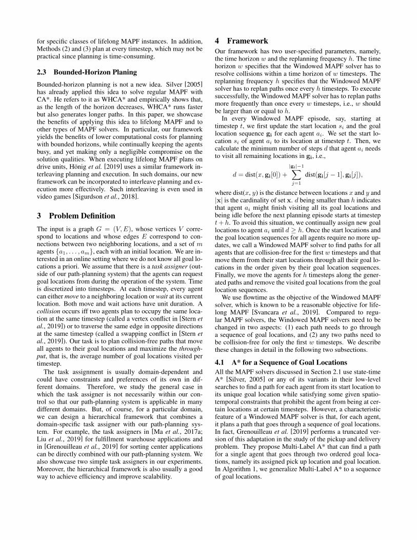
4.3 Behavior of Our FrameworkWe first claim that, in lifelong MAPF, resolving collisions fora longer planning horizon does not necessarily result in bettersolutions. Below is such an example.Example 1. Figure 2(a) shows a 3-agent example with w = 4timesteps and h = 2 timesteps. At timestep 0, all agents fol-low their shortest paths as no collisions will occur for thefirst 4 timesteps. Then at timestep 2, a3 reaches its goal lo-cation and is assigned a new goal location. This time, a1and a3 will collide at cell B at timestep 3. So a1 is forcedto wait for one timestep. However, if we solve this examplewith w = 8 timesteps and h = 2 timesteps, as shown inFigure 2(b), we could generate paths that include more waitactions. At timestep 0, the solver finds a collision between a1and a2 at cell A at timestep 7 and thus forces a2 to wait forone timestep. Then, at timestep 2, the solver finds a collisionbetween a1 and a3 at cell B at timestep 3 and forces a3 towait for one timestep. The number of total wait actions is 2.

Similar cases are also found in our experiments: sometimesour framework with smaller w achieves higher throughputthan the one with larger w. All of these cases support ourclaim that, in lifelong MAPF, resolving all collisions in theentire horizon may often do so unnecessarily, which is differ-ent from regular MAPF. Nevertheless, the bounded-horizonmethod also has a drawback - using a too small value for wmay generate deadlocks, as shown in Example 2.Example 2. consider the example shown in Figure 2(c) withw = 2 timesteps and h = 2 timesteps and assume that we use

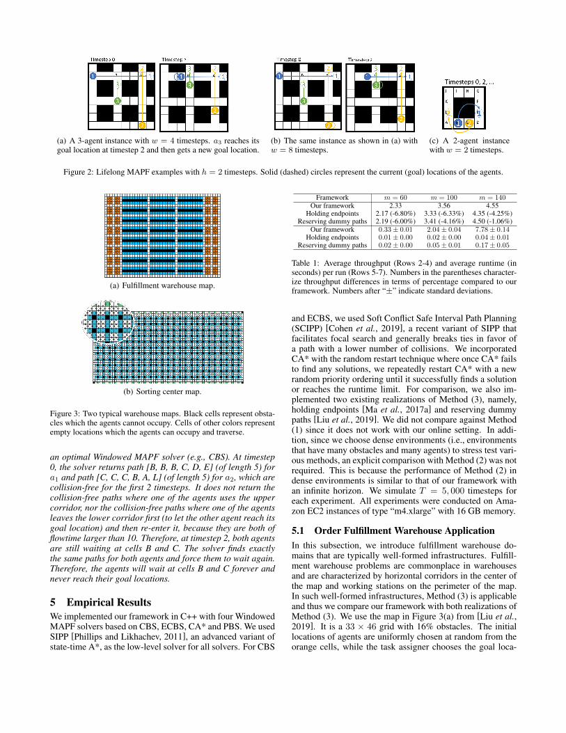
(a) A 3-agent instance with w = 4 timesteps. a3 reaches itsgoal location at timestep 2 and then gets a new goal location.

(b) The same instance as shown in (a) withw = 8 timesteps.

(c) A 2-agent instancewith w = 2 timesteps.

Figure 2: Lifelong MAPF examples with h = 2 timesteps. Solid (dashed) circles represent the current (goal) locations of the agents.

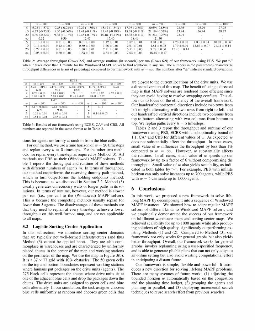
(a) Fulfillment warehouse map.

(b) Sorting center map.

Figure 3: Two typical warehouse maps. Black cells represent obsta-cles which the agents cannot occupy. Cells of other colors representempty locations which the agents can occupy and traverse.

an optimal Windowed MAPF solver (e.g., CBS). At timestep0, the solver returns path [B, B, B, C, D, E] (of length 5) fora1 and path [C, C, C, B, A, L] (of length 5) for a2, which arecollision-free for the first 2 timesteps. It does not return thecollision-free paths where one of the agents uses the uppercorridor, nor the collision-free paths where one of the agentsleaves the lower corridor first (to let the other agent reach itsgoal location) and then re-enter it, because they are both offlowtime larger than 10. Therefore, at timestep 2, both agentsare still waiting at cells B and C. The solver finds exactlythe same paths for both agents and force them to wait again.Therefore, the agents will wait at cells B and C forever andnever reach their goal locations.

5 Empirical ResultsWe implemented our framework in C++ with four WindowedMAPF solvers based on CBS, ECBS, CA* and PBS. We usedSIPP [Phillips and Likhachev, 2011], an advanced variant ofstate-time A*, as the low-level solver for all solvers. For CBS

Framework m = 60 m = 100 m = 140Our framework 2.33 3.56 4.55

Holding endpoints 2.17 (-6.80%) 3.33 (-6.33%) 4.35 (-4.25%)Reserving dummy paths 2.19 (-6.00%) 3.41 (-4.16%) 4.50 (-1.06%)

Our framework 0.33± 0.01 2.04± 0.04 7.78± 0.14Holding endpoints 0.01± 0.00 0.02± 0.00 0.04± 0.01

Reserving dummy paths 0.02± 0.00 0.05± 0.01 0.17± 0.05

Table 1: Average throughput (Rows 2-4) and average runtime (inseconds) per run (Rows 5-7). Numbers in the parentheses character-ize throughput differences in terms of percentage compared to ourframework. Numbers after “±” indicate standard deviations.

and ECBS, we used Soft Conflict Safe Interval Path Planning(SCIPP) [Cohen et al., 2019], a recent variant of SIPP thatfacilitates focal search and generally breaks ties in favor ofa path with a lower number of collisions. We incorporatedCA* with the random restart technique where once CA* failsto find any solutions, we repeatedly restart CA* with a newrandom priority ordering until it successfully finds a solutionor reaches the runtime limit. For comparison, we also im-plemented two existing realizations of Method (3), namely,holding endpoints [Ma et al., 2017a] and reserving dummypaths [Liu et al., 2019]. We did not compare against Method(1) since it does not work with our online setting. In addi-tion, since we choose dense environments (i.e., environmentsthat have many obstacles and many agents) to stress test vari-ous methods, an explicit comparison with Method (2) was notrequired. This is because the performance of Method (2) indense environments is similar to that of our framework withan infinite horizon. We simulate T = 5, 000 timesteps foreach experiment. All experiments were conducted on Ama-zon EC2 instances of type “m4.xlarge” with 16 GB memory.

5.1 Order Fulfillment Warehouse ApplicationIn this subsection, we introduce fulfillment warehouse do-mains that are typically well-formed infrastructures. Fulfill-ment warehouse problems are commonplace in warehousesand are characterized by horizontal corridors in the center ofthe map and working stations on the perimeter of the map.In such well-formed infrastructures, Method (3) is applicableand thus we compare our framework with both realizations ofMethod (3). We use the map in Figure 3(a) from [Liu et al.,2019]. It is a 33 × 46 grid with 16% obstacles. The initiallocations of agents are uniformly chosen at random from theorange cells, while the task assigner chooses the goal loca-

w m = 200 m = 300 m = 400 m = 500 m = 600 m = 700 m = 800 m = 900 m = 10005 6.22 (-1.57%) 9.28 (-0.93%) 12.27 (-1.56%) 15.17 (-1.84%) 17.97 (-2.35%) 20.69 (-2.85%) 23.36 25.79 27.95

10 6.27 (-0.75%) 9.36 (-0.06%) 12.41 (-0.41%) 15.43 (-0.19%) 18.38 (-0.11%) 21.19 (-0.52%) 23.94 26.44 28.7720 6.30 (-0.22%) 9.38 (+0.16%) 12.45 (-0.07%) 15.48 (+0.12%) 18.38 (-0.11%) 21.24 (-0.26%) 23.91 - -∞ 6.32 9.36 12.46 15.46 18.40 21.30 - - -5 0.13± 0.00 0.31± 0.00 0.61± 0.00 1.12± 0.01 1.87± 0.01 3.01± 0.01 4.73± 0.02 7.30± 0.04 10.97± 0.06

10 0.16± 0.00 0.42± 0.00 0.89± 0.00 1.66± 0.01 2.91± 0.01 4.81± 0.02 7.79± 0.04 12.66± 0.07 21.31± 0.1420 0.22± 0.00 0.61± 0.00 1.36± 0.01 2.71± 0.01 5.11± 0.03 9.28± 0.06 17.46± 0.14 - -∞ 0.28± 0.00 0.80± 0.01 1.83± 0.01 3.84± 0.03 7.63± 0.06 16.16± 0.17 - - -

Table 2: Average throughput (Rows 2-5) and average runtime (in seconds) per run (Rows 6-9) of our framework using PBS. We put “-”when it takes more than 1 minute for the Windowed MAPF solver to find solutions in any run. The numbers in the parentheses characterizethroughput differences in terms of percentage compared to our framework with w =∞. The numbers after “±” indicate standard deviations.

ECBSw m = 200 m = 300 m = 400 m = 500 m = 6005 6.23 (-1.21%) 9.17 (-1.47%) 12.03 (-2.03%) 14.79 (-2.68%) 17.28∞ 6.31 9.31 12.28 15.20 -5 0.26± 0.00 0.64± 0.00 1.27± 0.01 2.37± 0.02 4.22± 0.10∞ 1.81± 0.01 5.09± 0.03 11.48± 0.09 23.47± 0.22 -

CA* CBSw m = 200 m = 300 m = 400 w m = 100 m = 2005 6.17 (-0.48%) 9.12 (-0.35%) - 5 3.17 -∞ 6.20 9.16 - ∞ - -5 0.21± 0.01 1.07± 0.10 - 5 0.14± 0.03 -∞ 0.84± 0.02 2.58± 0.12 - ∞ - -

Table 3: Results of our framework using ECBS, CA* and CBS. Allnumbers are reported in the same format as in Table 2.

tions for agents uniformly at random from the blue cells.For our method, we use a time horizon of w = 20 timesteps

and replan every h = 5 timesteps. For the other two meth-ods, we replan every timestep, as required by Method (3). Allmethods use PBS as their (Windowed) MAPF solvers. Ta-ble 1 reports the throughput and runtime of these methodswith different numbers of agents m. In terms of throughput,our method outperforms the reserving dummy path method,which in turn outperforms the holding endpoints method.This is because, as we discussed in Section 2.2, Method (3)usually generates unnecessary waits or longer paths in its so-lutions. In terms of runtime, however, our method is slowerper run (i.e., per call to the (Windowed) MAPF solver).This is because the competing methods usually replan forfewer than 5 agents. The disadvantages of these methods arethat they need to replan at every timestep, achieve a lowerthroughput on this well-formed map, and are not applicableto all maps.

5.2 Logistic Sorting Center ApplicationIn this subsection, we introduce sorting center domainsthat are typically not well-formed infrastructures (and thusMethod (3) cannot be applied here). They are also com-monplace in warehouses and are characterized by uniformlyplaced chutes in the center of the map and working stationson the perimeter of the map. We use the map in Figure 3(b).It is a 37 × 77 grid with 10% obstacles. The 50 green cellson the top and bottom boundaries represent working stationswhere humans put packages on the drive units (agents). The275 black cells represent the chutes where drive units sit atone of the adjacent blue cells and drop the packages down thechutes. The drive units are assigned to green cells and bluecells alternately. In our simulation, the task assigner choosesblue cells uniformly at random and chooses green cells that

are closest to the current locations of the drive units. We usea directed version of this map. The benefit of using a directedmap is that MAPF solvers are rendered more efficient sincethey can avoid having to resolve swapping conflicts. This al-lows us to focus on the efficiency of the overall framework.Our handcrafted horizontal directions include two rows fromleft to right alternating with two rows from right to left, andour handcrafted vertical directions include two columns fromtop to bottom alternating with two columns from bottom totop. We replan paths every h = 5 timesteps.

Tables 2 and 3 report the throughput and runtime of ourframework using PBS, ECBS with a suboptimality bound of1.1, CA* and CBS for different values of w. As expected, wdoes not substantially affect the throughput. In most cases,small value of w influences the throughput by less than 1%compared to w = ∞. However, w substantially affectsthe runtime. In all cases, small value of w speeds up ourframework by up to a factor of 6 without compromising thethroughput. Small value of w also yields scalability, as indi-cated in both tables by “-”. For example, PBS with infinitehorizon can only solve instances up to 700 agents, while PBSwith w = 5 can scale up to 1,000 agents.

6 ConclusionsIn this work, we proposed a new framework to solve life-long MAPF by decomposing it into a sequence of WindowedMAPF instances. We showed how to adapt regular MAPFsolvers of different kinds to Windowed MAPF solvers, andwe empirically demonstrated the success of our frameworkon fulfillment warehouse maps and sorting center maps. Weachieved scalability for up to 1000 agents while also produc-ing solutions of high quality, significantly outperforming ex-isting Methods (1) and (2). Compared to Method (3), ourframework not only works for general graphs but also yieldsbetter throughput. Overall, our framework works for generalgraphs, invokes replanning using a user-specified frequency,and is able to generate pliable plans that can not only adapt toan online setting but also avoid wasting computational effortin anticipating a distant future.

Our framework is simple, flexible and powerful. It intro-duces a new direction for solving lifelong MAPF problems.There are many avenues of future work: (1) adjusting thebounded horizon w automatically based on the congestionand the planning time budget, (2) grouping the agents andplanning in parallel, and (3) deploying incremental searchtechniques to reuse search effort from previous searches.

References[Barer et al., 2014] Max Barer, Guni Sharon, Roni Stern, and Ariel

Felner. Suboptimal variants of the conflict-based search algo-rithm for the multi-agent pathfinding problem. In Proceedingsof the 7th Annual Symposium on Combinatorial Search (SoCS),pages 19–27, 2014.

[Cap et al., 2015] Michal Cap, Jirı Vokrınek, and AlexanderKleiner. Complete decentralized method for on-line multi-robottrajectory planning in well-formed infrastructures. In Proceed-ings of the 25th International Conference on Automated Planningand Scheduling (ICAPS), pages 324–332, 2015.

[Cohen et al., 2019] Liron Cohen, Tansel Uras, T. K. Satish Kumar,and Sven Koenig. Optimal and bounded-suboptimal multi-agentmotion planning. In Proceedings of the 12th International Sym-posium on Combinatorial Search (SoCS), pages 44–51, 2019.

[Grenouilleau et al., 2019] Florian Grenouilleau, Willem-Jan vanHoeve, and John N. Hooker. A multi-label A* algorithm formulti-agent pathfinding. In Proceedings of the 29th InternationalConference on Automated Planning and Scheduling (ICAPS),pages 181–185, 2019.

[Honig et al., 2018] Wolfgang Honig, James A. Preiss, T. K. SatishKumar, Gaurav S. Sukhatme, and Nora Ayanian. Trajectory plan-ning for quadrotor swarms. IEEE Transactions on Robotics,34(4):856–869, 2018.

[Honig et al., 2019] Wolfgang Honig, Scott Kiesel, Andrew Tinka,Joseph W. Durham, and Nora Ayanian. Persistent and robust ex-ecution of MAPF schedules in warehouses. IEEE Robotics andAutomation Letters, 4(2):1125–1131, 2019.

[Kou et al., 2020] Ngai Meng Kou, Cheng Peng, Hang Ma,T. K. Satish Kumar, and Sven Koenig. Idle time optimization fortarget assignment and path finding in sortation centers. In Pro-ceedings of the 34th AAAI Conference on Artificial Intelligence(AAAI), 2020.

[Liu et al., 2019] Minghua Liu, Hang Ma, Jiaoyang Li, and SvenKoenig. Task and path planning for multi-agent pickup and de-livery. In Proceedings of the 18th International Conference onAutonomous Agents and MultiAgent Systems (AAMAS), pages1152–1160, 2019.

[Ma et al., 2017a] Hang Ma, Jiaoyang Li, T. K. Satish Kumar, andSven Koenig. Lifelong multi-agent path finding for online pickupand delivery tasks. In Proceedings of the 16th InternationalConference on Autonomous Agents and MultiAgent Systems (AA-MAS), pages 837–845, 2017.

[Ma et al., 2017b] Hang Ma, Jingxing Yang, Liron Cohen,T. K. Satish Kumar, and Sven Koenig. Feasibility study: Movingnon-homogeneous teams in congested video game environments.In Proceedings of the 13th AAAI Conference on Artificial Intelli-gence and Interactive Digital Entertainment (AIIDE), pages 270–272, 2017.

[Ma et al., 2019] Hang Ma, Daniel Harabor, Peter J. Stuckey,Jiaoyang Li, and Sven Koenig. Searching with consistent pri-oritization for multi-agent path finding. In Proceedings of the33rd AAAI Conference on Artificial Intelligence (AAAI), pages7643–7650, 2019.

[Morris et al., 2016] Robert Morris, Corina S. Pasareanu,Kasper Søe Luckow, Waqar Malik, Hang Ma, T. K. SatishKumar, and Sven Koenig. Planning, scheduling and monitoringfor airport surface operations. In AAAI Workshop on Planningfor Hybrid Systems, 2016.

[Nguyen et al., 2017] Van Nguyen, Philipp Obermeier, Tran CaoSon, Torsten Schaub, and William Yeoh. Generalized target as-signment and path finding using answer set programming. InProceedings of the 26th International Joint Conference on Artifi-cial Intelligence (IJCAI), pages 1216–1223, 2017.

[Pearl and Kim, 1982] Judea Pearl and Jin H Kim. Studies in semi-admissible heuristics. IEEE Transactions on Pattern Analysis andMachine Intelligence, PAMI-4(4):392–399, 1982.

[Phillips and Likhachev, 2011] Mike Phillips and MaximLikhachev. SIPP: safe interval path planning for dynamicenvironments. In Proceedings of the IEEE International Con-ference on Robotics and Automation (ICRA), pages 5628–5635,2011.

[Sharon et al., 2015] Guni Sharon, Roni Stern, Ariel Felner, andNathan R. Sturtevant. Conflict-based search for optimal multi-agent pathfinding. Artificial Intelligence, 219:40–66, 2015.

[Sigurdson et al., 2018] Devon Sigurdson, Vadim Bulitko, WilliamYeoh, Carlos Hernandez, and Sven Koenig. Multi-agent pathfind-ing with real-time heuristic search. In Proceedings of the IEEEConference on Computational Intelligence and Games (CIG),pages 1–8, 2018.

[Silver, 2005] David Silver. Cooperative pathfinding. In Proceed-ings of the 1st Artificial Intelligence and Interactive Digital En-tertainment Conference (AIIDE), pages 117–122, 2005.

[Standley, 2010] Trevor Scott Standley. Finding optimal solutionsto cooperative pathfinding problems. In Proceedings of the 24thAAAI Conference on Artificial Intelligence (AAAI), pages 173–178, 2010.

[Stern et al., 2019] Roni Stern, Nathan R. Sturtevant, Ariel Felner,Sven Koenig, Hang Ma, Thayne T. Walker, Jiaoyang Li, DorAtzmon, Liron Cohen, T. K. Satish Kumar, Roman Bartak, andEli Boyarski. Multi-agent pathfinding: Definitions, variants, andbenchmarks. In Proceedings of the 12th International Symposiumon Combinatorial Search (SoCS), pages 151–159, 2019.

[Svancara et al., 2019] Jirı Svancara, Marek Vlk, Roni Stern, DorAtzmon, and Roman Bartak. Online multi-agent pathfinding. InProceedings of the 33rd AAAI Conference on Artificial Intelli-gence (AAAI), pages 7732–7739, 2019.

[Veloso et al., 2015] Manuela M. Veloso, Joydeep Biswas, BrianColtin, and Stephanie Rosenthal. Cobots: Robust symbiotic au-tonomous mobile service robots. In Proceedings of the 24th In-ternational Joint Conference on Artificial Intelligence (IJCAI),pages 4423–4429, 2015.

[Wan et al., 2018] Qian Wan, Chonglin Gu, Sankui Sun, MengxiaChen, Hejiao Huang, and Xiaohua Jia. Lifelong multi-agent pathfinding in a dynamic environment. In Proceedings of the 15thInternational Conference on Control, Automation, Robotics andVision (ICARCV), pages 875–882, 2018.

[Wurman et al., 2007] Peter R. Wurman, Raffaello D’Andrea, andMick Mountz. Coordinating hundreds of cooperative, au-tonomous vehicles in warehouses. In Proceedings of the 22ndAAAI Conference on Artificial Intelligence (AAAI), pages 1752–1760, 2007.

[Yu and LaValle, 2013] Jingjin Yu and Steven M. LaValle. Struc-ture and intractability of optimal multi-robot path planning ongraphs. In Proceedings of the 27th AAAI Conference on ArtificialIntelligence (AAAI), pages 1444–1449, 2013.