Lifecycle-Consistent Female Labor Supply with Nonlinear Taxes:

Evidence from Unobserved Effects Panel Data Models with Censoring, Selection and Endogeneity

Anil Kumar*

Senior Research Economist and Advisor Research Department

Federal Reserve Bank of Dallas anil.kumar@dal.frb.org

May, 2012

Abstract

This paper uses the PSID from 1979-2007 to estimate lifecycle-consistent labor supply elasticities of U.S. females with nonlinear taxes, in a two-stage budgeting framework. The paper is the first to estimate U.S. female labor supply models using semiparametric unobserved effects panel data methods with censoring, selection and endogeneity. The paper finds that female labor supply elasticities, particularly on the intensive margin, are sensitive to both the method used to account for unobserved effects and to economic assumptions regarding lifecycle behavior. The estimated lifecycle-consistent uncompensated wage elasticity for U.S. females from the correlated random effects model with instrumental variables is 0.56 on the extensive margin and 0.31 on the intensive margin, implying an overall wage elasticity of 0.87. In comparison, fixed effects models yield an overall wage elasticity of 0.77, substantially smaller than pooled panel models. Keywords: Taxes and Female Labor supply, Lifecycle labor Supply, Fixed Effects models with censoring, selection, and endogeneity JEL Numbers: J22, H24, C14, C23, C24 *Senior Research Economist and Advisor, Research Department, Federal Reserve Bank of Dallas. Previous versions if this paper were also circulated under two different titles: (1) “Lifecycle Consistent Estmiation of Female Labor Supply” and (2) “Taxes, Deadweight Loss and Intertemporal Labor Supply: Evidence from Panel Data”.The views expressed here are those of the author and do not necessarily reflect those of the Federal Reserve Bank of Dallas or the Federal Reserve System. I am grateful to Gary Engelhardt for his constant encouragement and generous support during this research. I thank Soren Blomquist, Monica Singhal, Tom Kniesner, Dan Black, Duke Kao, Jeffrey Kubik, Jan Ondrich and seminar participants at Syracuse University, Miami University, Federal Reserve Bank of Dallas, RAND Corporation and Institute of Social Research, University of Michigan, conference participants at the 99th Annual Conference on Taxation in Boston, and the 13th International Panel Data Conference in Cambridge, England for helpful discussions and insightful comments on previous versions. I am fully responsible for any errors.

2

1. Introduction

Following a sustained increase since the 1970’s, the recent decline in labor force

participation of married women has led to concerns that they are opting out of the labor

force (Juhn and Potter (2006), Macunovich and Pegula (2010)).1 With looming retirement of

baby boomers and a projected decline in the overall labor force participation rate, policies

aimed at stemming the exit of married females from the labor force could soon assume

added significance. Central to the design of such policies and evaluation of their welfare

costs is the female labor supply elasticity which remains an active area of research in public

finance and labor economics. Although there is broad agreement that female labor supply is

more elastic than male’s, consensus remains elusive on exactly how responsive females are

to tax and wage changes. More accurate estimates of the female labor supply elasticity are

also necessary to estimate the impact of fundamental tax reforms, back on the public policy

agenda due to growing concerns about the long-term sustainability of the U.S. fiscal deficit.

There is a long literature on taxation and female labor supply but gaps remain. Much

of the previous literature estimating within-period Marshallian labor supply elasticities for

U.S. females, incorporating nonlinear taxes, has primarily estimated static models assuming

myopic behavior and perfectly constrained capital markets.2 Estimates of within-period

elasticities from purely static models are not lifecycle-consistent and can be inaccurate if

1 Unless otherwise indicated all references to female labor supply in this paper refers only to married women. For recent research on single women, see Meyer and Rosenbaum (2001), Eissa and Liebman (1996) among others. 2 For example Hausman (1980), Hausman (1981), Moffitt (1984), Eissa (1995), Eissa (1995b), Eissa (1996) , Eissa and Hoynes (2004), Eissa and Hoynes (2005), Triest (1990), Blomquist and Hansson-Brusewitz (1990), van Soest et al. (1990), Heim (2007), Heim (2009), Kumar (2010) .

3

households can transfer assets across periods (Blundell and Macurdy (1999), Blundell and

Walker (1986)).

Estimating lifecycle-consistent female labor supply specification also forms a crucial

first step in the well-known two-stage budgeting framework to recover intertemporal

preferences if taxes are nonlinear and the intertemporal budget constraint is nonseparable.

Presence of nonlinear taxes can invalidate the widely used -constant labor supply

specifications ((Blomquist (1985), Blundell and Macurdy (1999), Ziliak and Kniesner

(1999)), while econometric specifications consistent with two stage budgeting remain valid

and can be used to estimate life-cycle consistent within-period female labor supply

following which intertemporal preference parameters can be recovered. Blundell and Walker

(1986), Blundell et al. (1993), Blundell et al. (1998) used two-stage budgeting

specifications to estimate lifecycle-consistent elasticities for British females. Aronsson and

Wikström (1994) estimated lifecycle-consistent of family labor supply with nonlinear taxes

using Swedish cross section data. Ziliak and Kniesner (1999) used the PSID to estimate

lifecycle-consistent labor supply elasticities in the presence of nonlinear taxes for a sample

of U.S. men. Papers that estimated lifecycle labor supply models for U.S. females, in

general, ignored complications caused by nonlinear taxation.3 Studies that accounted

carefully for nonlinear taxes, did not estimate lifecycle-consistent two-stage budgeting

specifications.

3Heckman and Macurdy (1980) and Kimmel and Kniesner (1998) estimated intertemporal elasticities for US females using a lifecycle model but ignored taxation. Other papers that have estimated lifecycle models for U.S. females ignoring taxes include Eckstein and Wolpin (1989), Jakubson (1988), Johnson and Pencavel (1984), Lilja (1986), Lundberg (1988), Zabel (1997) also estimated -constant female labor supply models without taxes.

4

In estimating static specifications, previous literature on taxes and female labor

supply in the U.S. used primarily cross-sectional rather than panel data.4 It is difficult to

account comprehensively for unobserved heterogeneity in female labor supply behavior

using cross-section data.5 Estimating unobserved effects models of female labor supply with

censoring and selection, has additional challenges, as simple fixed effects models do not

work due to incidental parameters problems; first differencing to remove the fixed effects is

not possible since the model is nonlinear (Neyman and Scott (1948)).

This paper makes two contributions to the existing body of work on female labor

supply. First, it uses the PSID from 1979-2007 to estimate within-period lifecycle consistent

labor supply elasticities of US females, in the presence of nonlinear taxation, in a two-stage

budgeting framework, in the spirit of papers such as Ziliak and Kniesner (1999) for US

males and (R Blundell et al., 1993) for British females.6 Second, the paper is the first to

estimate U.S. female labor supply models employing a variety of panel data estimation

methods including semiparametric fixed effects panel data methods with censoring,

selection and endogeneity, combining econometric approaches in Honoré (1992),

4Although panel data facilitates life-cycle consistent estimation, it is by no means absolutely necessary. Such specifications can be estimated even using cross-section data (see MaCurdy (1983), Blundell and Walker (1986)). 5Among recent papers on female labor supply elasticity, Devereux (2004) used repeated cross-section data from the Census IPUMS and used a grouping strategy to estimate static specifications of female labor supply with group fixed effects. Blau and Kahn (2007) and Heim (2007), who find compelling evidence that female labor supply elasticities are in a long term decline and converging towards men, estimated static models using a time series of cross-section data from the CPS. Gelber and Mitchell (2011) used fixed effects panel data model to estimate the hours elasticity with respect to net-of-tax-rate for single women of 0.53 using PSID 1975-2004. 6 In line with most other studies on female labor supply with nonlinear taxes, this paper estimates a secondary earners female labor supply model, in a unitary rather than collective framework, where wives, being secondary earners, make labor supply decisions conditional on husbands having made their labor supply choices. See Chiappori (1988), Fortin and Lacroix (1997), Apps and Rees (1997), Blundell et al. (2007) , Cherchye and Vermeulen (2008), Donni (2003), among others, for collective models of labor supply.

5

Kyriazidou (1997), Blundell and Powell (2007), Blundell and Powell (2004), (Charlier et al.,

2001), Papke and Wooldridge (2008), Wooldridge (2009) and Semykina and Wooldridge

(2010).

In many respects this paper is similar in spirit to three other papers which carefully

examined the sensitivity of female labor supply estimates to a variety of different

specifications: Mroz (1987), Jakubson (1988), and Zabel (1997). This paper differs from all

these three papers. While Mroz (1987) restricted analysis to just 1975 wave of the PSID,

Jakubson (1988), and Zabel (1997) used panel data from the PSID but estimated -constant

random and fixed effects Tobit models without taxes, ignoring the potential bias due to the

incidental parameters problem as well as complications due to nonlinear taxation.

There are three primary findings. First, female labor supply elasticity estimates,

particularly on the intensive margin, are sensitive to estimating unobserved effects

specifications. Fixed effects models yield participation wage elasticity of 0.43 compared

with 0.56 from both simple pooled panel models without unobserved effects and Correlated

random effects (CRE) specifications.7 Intensive margin elasticities, however, are more

sensitive to accounting for unobserved effects; fixed effects models and CRE specifications

produce much smaller and insignificant hours elasticities than pooled panel models.

Second, estimates of wage elasticity are somewhat sensitive to the choice of a more

general lifecycle-consistent framework applicable under nonlinear taxes versus a static

model, underscoring the need to account for lifecycle factors in female labor supply. In the

CRE specification with instrumental variables, the estimated lifecycle-consistent wage

7 This is different from the results for single women in Gelber and Mitchell (2011) who found that elasticities from fixed effects models were 50% larger than those without fixed effects.

6

elasticity on the extensive margin is 0.56, compared with 0.46 from the static model. On the

intensive margin, estimated lifecycle-consistent wage elasticity is 0.31 from the CRE

specification, while the static model yields a much smaller elasticity of 0.13. However,

given the large standard errors, the estimates are statistically indistinguishable.

Finally, the paper does not find evidence of significant difference in estimated

elasticities across lifecycle-consistent models applicable to linear taxes that condition on net

saving vis-à-vis models consistent with joint nonlinear labor and capital income taxes.8

Overall, the results indicate that the choice of econometric specification and economic

assumptions regarding lifecycle behavior can have implications for the estimated impact of

tax and transfer policies on female labor supply. The lifecycle-consistent wage elasticity

from the correlated random effects (CRE) model with instrumental variables is 0.56 on the

extensive margin and 0.31 on the intensive margin, implying an overall wage elasticity of

0.87. Fixed effects models yield an overall wage elasticity of 0.77 compared with an

elasticity of greater than one from pooled panel models.

This paper is organized as follows. Section 2 presents a brief theoretical framework

for married female labor supply in the presence of joint non-linear capital and labor income

taxation, and outlines the reasons for the use of two-stage budgeting. Section 3 describes the

econometric specification. Section 4 provides a brief description of the data and

construction of the key variables: wage, income, assets and taxes. Section 5 discusses the

results. There is a brief conclusion.

2. Theoretical Framework

8 Ziliak and Kniesner (1999) found negative wage elasticity when conditioning on net saving.

7

In the benchmark static model labor supply model with taxes, the consumer

maximizes the current period utility function with respect to consumption and hours of

work

, ; (1)

subject to the static budget constraint,

, , , (2)

where indexes individuals and indexes time, is a vector of exogenous taste shifters

that include other demographic and economic characteristics, the hourly wage rate,

the nonlabor income. , , is the nonlinear tax function with adjusted gross income

; is the capital income from end of period 1 assets

at an interest rate of , deductions and the number of exemptions. Consumer’s

optimization problem yields a labor supply equation as a function of after-tax wage rate

which equals 1 with , the marginal tax rate, and virtual income :9

, ; (3)

In the lifecycle model, the consumer chooses consumption and hours of work to

maximize the expected present discounted value of utility:

, ; (4)

subject to the asset accumulation constraint

1 , , (5)

where and represents assets in period and 1, respectively.

9 More specifically where is the actual tax liability and is what it would have been if the entire earnings were taxed at the marginal tax rate.

8

Notice that the tax function incorporates joint nonlinear taxation of labor and capital

income. Three points to note about the lifecycle-consistent consumer’s optimization problem

are: (1) utility is intertemporally separable; (2) within period utility is weakly separable in

consumption and leisure; (3) due to joint nonlinear taxation of labor and capital income, the

budget constraint is nonseparable in goods and prices across periods.

2.1. Nonlinear Taxes Invalidate -Constant Labor Supply Function

As shown in Blomquist (1985), if both preferences and the budget constraint are

intertemporally separable then the only way wages in one period change demand for leisure

in another is through a wealth effect. If so, a common solution is to estimate -constant or

Frisch labor supply functions, where , the individual specific time invariant marginal utility

of wealth is a sufficient statistic for information in other periods and can be differenced

away using fixed effects panel data models Heckman and Macurdy (1980).

However, when taxes are nonlinear and the budget constraint is nonseparable in

goods and prices, wage changes in one period can affect labor supply in other periods by

impacting wages in those periods, in addition to the wealth effect. In other words, labor

supply in one period is a function of prices in other periods. Blomquist (1985) showed that

in the presence of nonlinear taxes, the marginal utility of wealth is no more a sufficient

statistic and -constant labor supply function fails to account for the nonseparabilities in the

budget constraint, but two-stage budgeting remains valid. Ziliak and Kniesner (1999) used

two-stage budgeting approach to estimate lifecycle-consistent labor supply elasticities for

US males. Such an approach has not been used to model lifecycle-consistent elasticities for

US married women.

2.2. Sufficient Statistics Under Two-Stage Budgeting

9

In a two stage budgeting framework, proposed by Gorman (1959), in the first-stage,

the consumer allocates total expenditure across periods to equate the marginal utility of

wealth. In the second-stage, she takes the allocation of wealth between periods as given,

and allocates between consumption and hours, like a standard static intratemporal problem,

conditional on and . In this framework, contains information on the past

decisions and tA represents the effect of future prices.

As shown in Blomquist (1985), in a two-stage budgeting framework, in the absence

of taxes or in the presence of a linear capital income tax that result in time separable budget

constraint, net saving 1 is a sufficient statistic for incorporating

information from other periods, where is the after tax rate of interest.

Instead, if taxes are nonlinear as they are in the U.S., then and can be used

as sufficient statistics that capture the adjustment in level of assets by the end of the period.

Alternatively, saving 1 and capital income can also serve as

sufficient statistics. Following Ziliak and Kniesner (1999) and using and as

sufficient statistic, lifecycle-consistent labor supply is a function of the after-tax wage rate

, and virtual lagged asset :10

, , ; (6)

3. Estimation and Identification

10Analogous to virtual income , following Ziliak and Kniesner (1999), the virtual lagged assets are defined as / . The reason why this adjustment is made to lagged assets and not to current period assets is, as explained in Ziliak and Kniesner (1999), that income on previous period assets figure into tax calculations.

10

Writing the desired labor supply in (6) as a latent variable , the baseline lifecycle-

consistent female labor supply specification in a world with nonlinear taxes becomes: 11

(7)

equals actual hours if 0 and 0 otherwise. is an individual specific

unobserved effect, is a mean zero error term.

What distinguishes the general lifecycle-consistent specification with nonlinear taxes

in (7) from more restrictive specifications with a linear capital income tax or from a static

model without possibility of transfer of assets across periods? If capital income taxes were

linear or there were no taxes, then virtual net saving could be used instead of and

in (7).12 If, on the other hand, the objective is to estimate a static model, virtual income

replaces and in (7) above.

A variety of approaches can be used to estimate the parameters of the labor supply

equation (7). Some methods account comprehensively for piecewise-linear budget set

underlying the derivation of the labor supply function (Burtless and Hausman (1978),

Hausman (1981), Heckman and MaCurdy (1982), Blomquist and Newey (2002), Heim

(2009), Kumar (2008), Kumar (2010), Liang (2011)). These methods, however, are not

easily amenable to fixed effects estimation with panel data. Therefore, in line with other

recent studies on female labor supply elasticities, this paper uses a simpler approach and

11Hereinafter denotes after-tax wage of workers as well as nonworkers with the nonworker’s missing wages replaced by after tax predicted wage . 12 To account for nonlinear taxes virtual net saving was calculated as the sum of net saving and a lump sum transfer akin to one used for virtual income i.e. 1 .

11

calculates the after-tax wage by linearizing the budget set at the observed marginal tax

rate (Hall (1973)) and then treating as endogenous.13

Tobit can be used to estimate (7) if wages for all females were available. Tobit-type

labor supply equations, however, are based on the premise of a continuous labor supply

schedule that constrains the parameters of the participation decision and the hours of work

decision to be identical and will be biased if participation and hours decisions are separate.

The paper, therefore, also estimates participation elasticities using Probit/Logit models with

an indicator for labor force participation, , replacing as the dependent variable in

(7). Elasticities on the intensive margin are obtained by estimating selection-corrected hours

equations, restricting the estimation sample to workers. Since Tobit/Probit/Logit model is

based on the entire sample, imputed wages are required for females out of the labor force.

3.1 Selection-Corrected Wage Equation to Predict Wages

Following the previous literature, unobserved wages in the Probit/Logit/Tobit-type

models are replaced by wage estimated from a selectivity-bias-corrected wage equation.14

The two-step Heckman type selection-corrected wage equation can be written as:

(8)

(9)

13An alternative approach of imputing the effective marginal tax rate from a differentiable smooth budget constraint methodology proposed in MaCurdy et al. (1990) and Ziliak and Kniesner (1999) was also followed but the results were similar. 14Using predicted wages for non-workers is standard in the literature on female labor supply with taxes. The primary condition for consistency is consistent estimates of the wage equation parameters Wales and Woodland (1980). Some earlier researchers used OLS to estimate the wage equation Hall (1973), Rosen (1976)). This strategy has been criticized on grounds of selectivity-bias in the wage equation Killingsworth and Heckman (1986); Wales and Woodland (1980). Many other studies use selectivity-bias adjusted wage predictions (Hausman (1980b); Bourguignon and Magnac (1990); Colombino and Del Boca (1990); Triest (1990); van Soest et al. (1990).

12

In the first step, a reduced form selection equation for labor force participation (8) is

estimated as a linear regression on a vector of variables, , consisting of power series in

age, education, race, unearned income and a dummy for the presence children under

seven years ( 7 , for each year, allowing the coefficients to vary by year. In the

second step, for each year, the wage equation (9) is estimated by regressing log of real wage,

on a vector of regressors consisting of all variables in except unearned income

and 7 - which act as exclusion restrictions- and inverse mills ratio term

, obtained from (8). The identifying assumption is, conditional on age, education

and other demographics, and 7 are correlated with the labor force participation

status but conditional on labor force participation, they are uncorrelated with wages.

3.2 Endogeneity, Instruments and Identification

Using panel data, this paper uses both cross-sectional and time-series variation in

wages, assets, and tax rates from 1979-2007 to identify the effect of taxes on labor supply.

The previous three decades spanned four major tax reforms in ERTA 1981, TRA 1986,

1993, and the Bush Tax Cuts of 2001. The time-series variation in marginal tax rates

induced by these reforms helps identify the wage effects as well as the coefficient on virtual

asset. The cross-sectional variation in after- tax wage, virtual income and assets, however is

likely to be endogenous for three reasons.

First, if taxes are progressive, the current period marginal tax rate is endogenous to

the choice of current period earnings and hours of work. Second, as noted by Eissa (1995),

the marginal tax rate is a nonlinear function of income and family size, and may be

correlated with underlying tastes for work that also may be correlated with income and

family size. The endogeneity of the marginal tax rate renders key variables, after tax wage,

13

1 and virtual lagged real net assets, , endogenous as they are

functions of the marginal tax rate, . And finally, the gross wage and current period

assets themselves may be endogenous as they may be potentially correlated with

unobserved tastes for work.

Instrumental Variables

This paper accounts for the potential endogeneity of , , and using

instrumental variables. After-tax real wage is instrumented with after-tax predicted real

wage, 1 , where is the predicted wage from the wage equation (9) and

is the first-dollar tax rate on household’s earnings.15 The identifying assumption is that

the first-dollar tax rate is correlated with the observed marginal tax rate but is otherwise

uncorrelated with hours of work.16

To further guard against potential endogeneity in contemporaneous values of the

paper follows Ziliak and Kniesner (1999) in using the second lag of i.e. as

instrument.17 Analogously, the second lag of / i.e.

is used as instrument for . With used to construct the instrument for ,

is used as an instrument for current real assets . In addition to

, , , the baseline instrument set also includes time dummies, the

15In the literature on nonlinear budget set estimation with taxes using maximum likelihood, gross wage and full income are treated as exogenous. However, both of these could be endogenous in a lifecycle model due to human capital accumulation factors. Also, first lags are not used as instruments due to potential first order serial correlation in the error term. 16 Other plausible instruments for the tax rate e.g. marginal tax rate on husband’s earnings based on 2000 hours a years were also used as instruments. The results were similar. 17Under the assumption of rational expectations, everything in the information set at time 1t and before is exogenous. So the twice-lagged value of the gross wage and full income are considered exogenous are valid for making instruments.

14

identifying assumption being that aggregate shocks are correlated with hours only through

the after tax wage and asset variables (MaCurdy (1981); Altonji (1986); Angrist (1991);

Ziliak and Kniesner (1999)).18

4. Data

The Panel Study of Income Dynamics (PSID) began in 1968, and is a longitudinal

data on a sample of U.S. individuals and their family units, collected annually from 1968 to

1996 and every other year since 1997. The sample consists of an unbalanced panel of 2210

married women surveyed in the PSID between 1979 and 2007, for a total of 14303

observations.19 Up to four lags of endogenous variables were used as instruments, and

therefore, the PSID waves used in the estimation sample range from 1983 to 2007 with 1982

to 2006 as reference years. In addition to the PSID data directly available from the Survey

Research Center, University of Michigan, the Cross-National Equivalent File for PSID

(PSID-CNEF) available from the Department of Policy Analysis and Management at

Cornell University were used to construct the key variables used in the paper ((Burkhauser

et al., 2001)).

Measurement of Key Variables

18 Analogously, ,the second lag of virtual net saving and time dummies are used as instruments in models applicable with linear capital income taxes and , and time dummies are used as instruments in the static specifications, where is constructed by replacing the actual marginal tax rate in with the first dollar tax rate. 19PSID collects most labor market information for the year before the survey year, so data 1979 to 2007 waves refer to years 1978 to 2006. Also since 1996, PSID surveyed individuals only once The main sample of PSID, i.e. excluding an oversample of low-income families, has 60368 observations on wives from 1979 and 2007. Restricting the age to 22-60 years olds resulted in 50675 observations. 14158 observations were dropped as wife or head was self-employed, head was a farmer, or household had own business, leaving 36517 observations. Further, 234 person years were excluded as they were deemed outliers using multivariate outlier detection criteria. 5899 observations from 1979-1982 were dropped as the instrument consisted of 4th lag of real asset. Finally 16089 person years were dropped due to missing data on one or more of the dependent variable, or the explanatory variables, or the instruments which consisted of 2nd, 3rd, and 4th lags of endogenous variables.

15

Wages

The PSID contains more than one measure of the wage rate. One measure can be

formed by dividing annual real earnings by the annual hours worked. This measure has

been found in the literature to induce division bias in labor supply estimates, yielding

parameter estimates inconsistent with theory (Ziliak and Kniesner (1999), Eklof and Sacklen

(2000), Engelhardt and Kumar (2007)). Following the Ziliak and Kniesner (1999), a self-

reported measure of wage is used, that does not require dividing annual labor income with

annual hours, and is free of division bias. For hourly workers the hourly wage directly

reported by workers was used. For salaried workers, the PSID asked the dollar amount they

received in salary and the pay period i.e. once a month, twice a month, or weekly. Assuming

that the salaried individual worked 40 hours a week, the dollar amount was divided by the

respective number of hours worked during the pay period. Nominal hourly wages are then

converted to real 2000 dollars by adjusting with the CPI (U). The log of real wage was used

to estimate a selection-corrected wage equation to impute real wages for married women out

of the labor force.

Nonlabor Income and Assets

Nonlabor income is calculated as the sum of head’s labor income and the

household’s asset income obtained from PSID-CNEF data. The method proposed in Ziliak

and Kniesner (1999) was used to calculate the assets at the household level. First, liquid

assets were calculated by capitalizing the first $200 of annual household asset income using

the one month CD rate while the amount above $200 was capitalized using the 3-month

treasury bill rate. Liquid assets were then added to home equity to calculate total household

asset. Home equity was calculated as the difference between self reported value of the house

16

and the remaining mortgage and principal amount. The remaining mortgage and principal

amount was not available for 1982; PSID-CNEF method was followed to impute the amount

by adding half the difference between 1983 and 1981 value to the 1981 value.

Taxes

The adjusted gross income was calculated as the sum of household’s pre-government

income and government transfer income both available from the PSID-CNEF data. The pre-

government income in PSID-CNEF is the sum of total family income from labor earnings,

asset income, private transfers such as child support and alimony, and private pensions.

Given the itemization status of the household from PSID, the dollar amount of itemized

deduction was imputed as the average of itemized deduction for different categories of

adjusted gross income from the NBER tax public use files obtained from IRS Statistics of

Income. Information on year, filing status, number of dependents, number of age

exemptions, household labor income, itemized deductions, and state was used to calculate

the federal, state, and payroll tax rates and tax liabilities using the NBER-TAXSIM

(Feenberg and Coutts (1993)). Federal, state, and payroll tax rates were then added to

calculate the overall marginal tax rate for each individual, for each year.

5. Results from Panel Data Models with Censoring, Selection, and Endogeneity

The paper estimates three types of elasticities: (1) participation elasticity using

Probit/Logit type model (2) intensive margin elasticities using selection-corrected hours

equation by restricting sample to labor force participants, and (3) Tobit-type models with

censoring to estimate total hours elasticity. All three labor supply models are estimated

using: (1) Pooled panel data model, (2) Fixed Effects (FE) model, and (3) Correlated

Random Effects (CRE) model. Further, each model is estimated first without instrumental

17

variables (IV) and with IV. The estimation details of various models are presented in

Appendix 1.

5.1 Participation Elasticities

Table 2 presents marginal effects and elasticities on the extensive margin with

respect to the three key variables in the lifecycle-consistent specification: after-tax wage,

virtual lagged asset and current asset. The upper panel contains the marginal effects while

the lower panel of each table presents the estimated elasticities. Table 2 shows that IV

estimates of marginal effects are larger than non-IV estimates. Among the three panel data

models, FE-Logit-IV model yields the smallest elasticity of 0.43 compared with 0.56 from

both the pooled panel and CRE-Probit-IV models, although, not statistically different..20

This pattern, however, does not apply to wealth elasticities as they are more or less

similar across different models. Adding up the lagged and current assets elasticities yields a

cumulative wealth elasticity of about -0.10 in both the pooled-Probit-IV and FE-Logit-IV

specification and -0.14 in the CRE-Probit-IV specification.21

The estimated wage elasticities from the three panel data specifications with IV in

columns (2), (4), and (6) are not precise enough to be statistically distinguishable. Indeed, a

Hausman-type specification test on a subset of coefficients on key variables- after-tax wage,

virtual lagged assets and current asset - had a p-value of 0.49 and failed to reject the CRE

20One limitation with fixed effects models is that average partial effects and therefore, elasticities are, in general, not identified, as the unobserved effects are not estimated (Wooldridge (2010), Abrevaya and Hsu (2011) Chernozhukov et al. (2009)). For the fixed effect logit, first the predicted probability of participating in the labor force was calculated conditional on a positive outcome for each individual. The mean of this predicted probability was used to calculate the adjustment factor for calculating marginal effects. Having calculated marginal effects, elasticities were calculated by multiplying with the ratio of mean wage to mean labor force participation. 21Cumulative one period dynamic response has been calculated as suggested in Stock and Watson (2007).

18

Probit-IV model in column (6) vis-à-vis FE-Logit-IV model in column (4).22 This is

interpreted as evidence in favor of the CRE-Probit specification (Hausman (1978)).

The instrumental variables have significant explanatory power in the first stage

regressions for all the three endogenous variables - after-tax wage, lagged asset and current

asset - as the p-values on a joint test of instruments were well below 0.05. The p-values on

the overidentification test, shown in the bottom panel, in columns (2) and (6) suggest that

overidentification restrictions cannot be rejected, and therefore the instruments are valid.

The p-value on the joint test of correlated random effect terms in column (6) indicates

rejection of the hypothesis that, the terms controlling for correlation between the unobserved

heterogeneity and the other model regressors are zero.

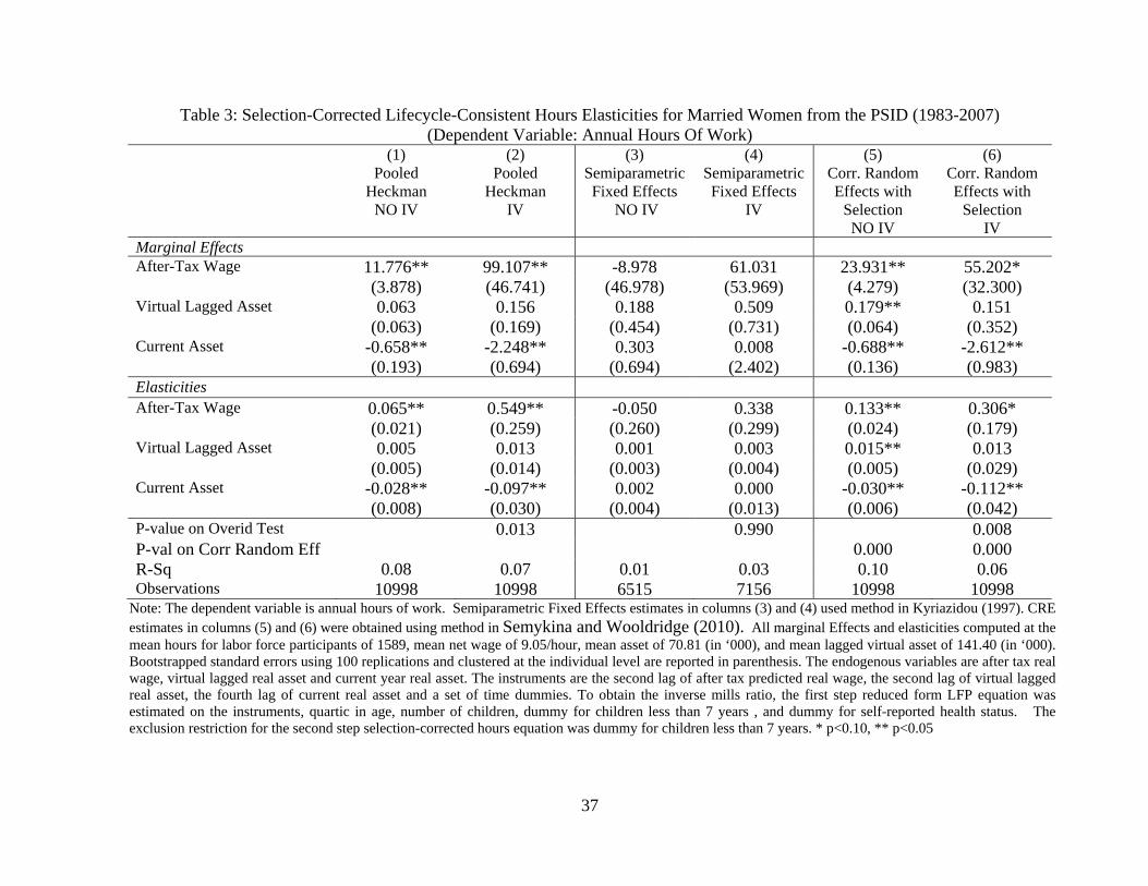
5.2 Intensive Margin Elasticities

The intensive margin results in Table 3 show a somewhat different pattern than those

in Table 2 as they are more sensitive to unobserved effects specifications. The wage

elasticity from the selection-corrected CRE-IV model in column (6) is about 44 percent

smaller than the pooled-Heckman-IV results in column (2), although the confidence

intervals around the estimates overlap. The estimated elasticity from instrumental variable

semiparametric FE-IV model in column (4) is 0.35 and not statistically significant. The

wealth elasticities on the intensive margin are similar to extensive margin estimates, with the

one period cumulative wealth elasticity in column (6) of -0.10. Assets elasticities from the

semiparametric FE-IV model are not significant. Given the large difference in estimated

22The Hausman test can fail if the difference between variance-covariance matrices of the efficient and consistent specification may not be positive semidefinite. A suggestion in (Jeffrey M. Wooldridge, 2010) page 331 is used to calculate the Hausman test statistic for only a subset of coefficients of primary interest, i.e. after-tax wage, virtual lagged asst and current asset.

19

elasticity between CRE-IV and FE-IV models, a Hausman-type specification test with a p-

value of 0.013 rejects the CRE-IV model in column (6) vis-à-vis the FE-IV model in column

(4).

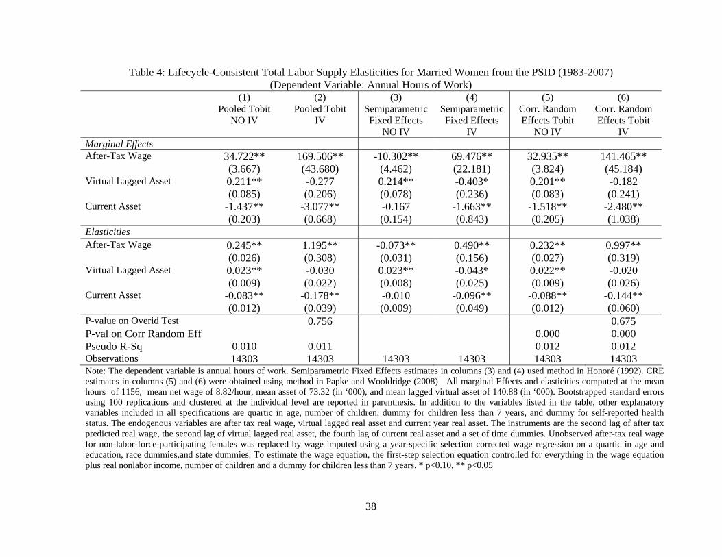
5.3 Total Hours Elasticities from Tobit-type Models with Panel Data

The overall hours elasticities obtained from the Tobit-type censored labor supply

models presented in Table 4 show that semiparametric FE-IV estimates in column (4) are

just about half of the CRE-Tobit-IV estimates in column (6).23 Wage elasticities from CRE-

Tobit-IV are similar to pooled-Tobit-IV estimates in column (2). A Hausman-type

specification test of CRE-Tobit-IV model in column (6) versus the fixed effects model in

column (4), yielded a negative test statistic. The total wage elasticity from the CRE-Tobit-IV

model in column (6) is 1 and the one period cumulative wealth elasticity is -0.16.

5.4 Sensitivity to economic assumptions regarding lifecycle behavior and taxes

By conditioning on lagged and current asset, labor supply models estimated in

Tables 2, 3, and 4 appropriately accounted for the realities of joint nonlinear taxation of

labor and capital income taxation. How do these estimated elasticities compare with models

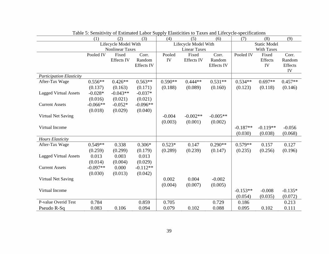
that apply only to linear tax settings or to static models? Columns (4), (5), and (6) of Table 5

present estimated elasticities from models that condition on virtual net savings and,

therefore, are consistent with assumptions of either no taxes or a linear capital income tax.

Columns (7), (8), and (9) present results from static models of female labor supply estimated

23Marginal effects in the semiparametric fixed effects models for nonlinear panel data are, in general not identified. However, the marginal and elasticities for such models in the paper are calculated by simply treating the estimated coefficients as marginal effects.

20

in much of the previous literature using cross-section data. For comparison, columns (1), (2),

and (3) reproduce participation elasticities from Table 2 and hours elasticities from Table 3.

Estimated elasticities are somewhat sensitive to economic assumption of a static

versus a lifecycle model. The CRE-Probit-IV estimate of the participation wage elasticity

from the static model in column (9) is 0.46, smaller than 0.56 from the general lifecycle-

consistent model in column (3). The static model, however, yields a larger estimate of

participation wage elasticity of 0.7 from the FE-Logit-IV model than the lifecycle-consistent

estimate of 0.43. Wealth elasticities in columns (1)-(3) are significantly larger than

responses due to increases in net savings from lifecycle model valid under linear taxes in

columns (4)-(6), but not much different from income elasticities from static model in

columns (7)-(9)

The intensive margin wage elasticities, in the lower panel, show a much different

pattern across the unobserved effects lifecycle-consistent and static models. Hours

elasticities from fixed effects as well as CRE static models are less than half those from

lifecycle consistent models and statistically insignificant.

Adding up the extensive and the intensive margins, lifecycle-consistent model with

nonlinear taxes and nonseparable budget constraint yields an overall wage elasticity of 0.87

from the CRE specification and 0.77 from the fixed effects model, although, the intensive

margin elasticities are not statistically different from zero. On the other hand, overall wage

elasticities from a model consistent with linear taxes and hence time-separable budget set are

0.82 from the CRE and 0.59 from a fixed effects model. The static model produces an

overall elasticity of 0.59 from the CRE and 0.86 from fixed effects. Figure 1 plots the

estimated uncompensated and compensated wage elasticities from different IV models.

21

5.5 Robustness to Regressors and Alternative Instruments

Tables 6 and 7 present results on robustness of lifecycle-consistent participation and

hours elasticities to inclusion of regressors and to use of alternative instruments. Results are

robust to controlling for a quadratic time trend in columns (3) and (4), and to accounting for

spouse’s wage in columns (7) and (8). Controlling for the unemployment rate to account for

business cycle effects in columns (5) and (6), however, yields markedly different results on

participation elasticities in the upper panel compared with the baseline model in columns (1)

and (2). Both participation elasticities and hours elasticties in the CRE model in column (6)

are insignificant when unemployment rate is included. A possible explanation could be that

the unemployment rate is mechanically correlated with participation and therefore an invalid

control in the upper panel of column (6).

Table 7 examines robustness to alternative instruments. Columns (1) and (2) drop the

time dummies from the baseline instrument set and use just the lags of the endogenous

variables evaluated at the first dollar tax rate and. Columns (3) and (4) reproduce the pooled-

IV and CRE-IV results with the baseline set of instrumental variables from Tables 2 and 3

that include time dummies as in Ziliak and Kniesner (1999). The p-values on

overidentifying restrictions in columns (3) and (4) confirm that time dummies are indeed

valid instruments.

Columns (5) and (6) present results using groups formed by interaction of whether or

not the individual had a high school diploma, year of birth category, and year as instruments

similar in spirit to Blundell et al. (1998).24 Columns (7) and (8) contain estimated

24Instruments were formed by interaction of 2 education groups, 4 year of birth groups, and 19 years.

22

elasticities using wage deciles by year groups as instruments, similar to Blau and Kahn

(2007). The estimated participation elasticities are largely robust to use of alternative

instruments. The point estimates of the intensive margin elasticity are substantially smaller

from the CRE-IV specification in column (8) compared with those in columns (4) and (6).

However, none of the elasticities in columns (4), (6), and (8) are statistically different from

each other. P-vlaues in the bottom panel indicate that overidentifying restrictions on

education by cohort by year groups in columns (5) and (6) and on wage deciles by year

groups in columns (7) and (8) are rejected.

5.6 Implied Deadweight Loss and Frisch Labor Supply Elasticity

Estimates of uncompensated wage and wealth elasticities from the lifecycle-

consistent specification can be used to calculate the deadweight loss from taxes and simulate

the efficiency costs of tax policy. Adding up the wage elasticities on the participation and

intensive margins, the overall wage elasticity from the CRE-IV specification is 0.87, while

summing wealth elasticity on the two margins yields an estimate of -0.23. The implied

compensated elasticity ( is 0.9.25

The well-known Harberger-Browning formula can then be used to simulate the

increase in deadweight loss from changes in tax policy (Harberger (1964), Browning

(1987)).26 Allowing the Bush tax to expire for married women filing jointly with total

25The compensated elasticity on labor supply can be recovered using the formula

where , , are the uncompensated wage, compensated wage, and wealth elasticity,

respectively. As the married womens’ earnings relative to assets 0.19, the compensated elasticity is

0.64. 26 Deadweight loss equals , where , is the marginal tax rate. This expression equals 0.028 if

0.25 and 0.034 if 0.27.

23

household earnings of $100,000 a year, for example, will lead to an increase in federal

income tax rate from 25% to 27%. The implied deadweight loss would go up from 3.8% of

earned income before the tax change to 4.6% after.27

The estimated elasticities can also be used to recover the -constant elasticity- by

using the formula , where is the intertemporal substitution

elasticity (Browning (2005)). An estimate of the intertemporal substitution elasticity is

needed to recover . With 0.008, is not much different from for most

plausible estimates of . Using an estimated of -0.69 from Blundell et al. (1993), the

implied for the lifecycle-consistent CRE specificationis 0.92, about the same as the

compensated elasticity.

5.7 Comparison with Elasticities of U.S. Married Women in the Previous Literature

The uncompensated overall wage elasticity of 0.87 and 0.76 from the CRE-IV and

fixed effects-IV models, respectively, although well within the range of estimates is similar

to the median estimate of 0.7-0.8 reported in two major survey papers by Killingsworth and

Heckman (1986) and Blundell and Macurdy (1999). Estimated total labor supply elasticities

are close to other papers using the PSID e.g. Hausman (1981), Hausman and Ruud (1984),

and Triest (1990) who reported wage elasticities of 0.9, 0.76, and 1 respectively. The

intensive margin elasticity of 0.30 from the CRE-IV model is very similar to Triest (1990).

27The calculation attempted here is at best a crude measure of deadweight loss from tax changes. Eissa et al. (2008) showed that the relevant tax rates for welfare cost calculations on the participation margins may be different. While the effective marginal tax is valid for the intensive margin, average rate is appropriate for the participation margin. Further, the calculation using labor supply elsticity ignores other margins of behavioral response i.e. effort, avoidance etc. A more comprehensive measure can be calculated using response on taxable income (Feldstein (1999), Saez et al. (2009)).

24

Elasticities in this paper are, however, substantially larger than from Mroz (1987) whose

estimated married women’s elasticities using the 1975 PSID were not much different from

prime age men’s.

Using non-PSID datasets, papers such as Cogan (1981), Rosen (1976)), Heckman

and Macurdy (1980), and Kimmel and Kniesner (1998) estimated total hours elasticities

larger than 2. Estimated elasticities are closer to those in Eissa (1995) who, using the CPS,

estimated a total hours elasticity of 0.8 for high income women with roughly half of it on the

extensive margin. The estimated participation elasticity of 0.56 from the CRE-IV model is

more than twice that of 0.27 found in Eissa and Hoynes (2004) while the intensive margin

elasticity is larger than 0.2 reported in Devereux (2004). Both participation and intensive

margin elasticities from the CRE specifications are within the range of those in Blau and

Kahn (2007) who found that participation elasticities declined from 0.58 to 0.28 from 1980

to 2000 while the hours elasticities dropped from 0.3 to 0.12. Heim (2009) also found a

similar decline with participation elasticities declining from 0.2 to 0.1 and participation

elasticities shrinking from 0.5 to 0.

6. Conclusion

Much of the previous literature on taxes and female labor supply in the U.S primarily

estimated static models assuming myopic behavior and perfectly constrained capital

markets. Estimates of within-period elasticities from purely static models are not lifecycle-

consistent and can be inaccurate if households can transfer assets across periods. Estimating

lifecycle-consistent specification of female labor supply in a two-stage budgeting framework

can also help recover intertemporal preferences in the presence of nonlinear taxes, when λ-

constant labor supply specifications are generally not valid. Despite their apparent

25

usefulness, lifecycle-consistent two-stage budgeting specifications incorporating nonlinear

taxes have not been estimated for female labor supply in the U.S.

This paper uses the PSID from 1979-2007 to estimate lifecycle-consistent labor

supply elasticities of U.S. females with nonlinear taxes, in a two-stage budgeting

framework. The paper is the first to estimate U.S. female labor supply models using

semiparametric unobserved effects panel data methods with censoring, selection and

endogeneity. The paper finds that female labor supply elasticities are sensitive to both the

method used to account for unobserved effects and to economic assumptions regarding

lifecycle behavior and taxes. Participation and hours wage elasticities are substantially

smaller for unobserved effects panel data models compared with pooled panel models.

The uncompensated wage elasticity from a lifecycle-consistent model with nonlinear

taxes and nonseparable budget constraint, using CRE model with instrumental variables, is

0.56 on the extensive margin and 0.31 on the intensive margin, implying an overall wage

elasticity of 0.87; fixed effects model yields an overall wage elasticity of 0.76 compared

with close to one from the pooled panel model. Overall wage elasticity from a model

consistent with linear taxes and hence time-separable budget set are not much different. The

static model, however, produces an overall elasticity of 0.58 from the CRE model and 0.85

from fixed effects.

Some important caveats apply to the results in the paper. First, like most previous

studies on taxes and labor supply, this paper estimates a secondary earners model of female

labor supply in a unitary rather than collective framework. Second, by linearizing the budget

set and adopting an instrumental variables approach, the paper has sidestepped

complications from modeling the entire budget set and ignored any biases due to

26

nonconvexities and fixed costs. Third, the estimated elasticities may be downward-biased as

the paper does not account for human capital accumulation (Keane (2011), Imai and Keane

(2004)). The model also does not account for optimization frictions which could cause

observed elasticities to be different from their structural estimates (Chetty (2009)). And

finally, marriage and fertility have been assumed to be exogenous. Addressing these features

in the context of a lifecycle-consistent female labor supply model with nonlinear taxes using

panel data is left to future research.

27

References

Abrevaya J, Hsu YC. Estimation of partial eff_ects in non-linear panel data models. Working Paper,Department of Economics, University of Missouri; 2011.

Altonji JG. Intertemporal Substitution in Labor Supply: Evidence from Micro Data. Journal of Political Economy 1986; 94; S176–s215.

Andersen EB. Asymptotic Properties of Conditional Maximum-Likelihood Estimators. Journal of the Royal Statistical Society. Series B (Methodological) 1970; 32; 283–301.

Angrist JD. Grouped-Data Estimation and Testing in Simple Labor-Supply Models. Journal of Econometrics 1991; 47; 243–266.

Apps PF, Rees R. Collective Labor Supply and Household Production. Journal of Political Economy 1997; 105; 178–190.

Arellano M, Honore B. 2001. Panel Data Models: Some Recent Developments. In: . Handbook of Econometrics. Volume 5. Elsevier Science, North-Holland; 2001. pp. 3229–3296.

Aronsson T, Wikström M. Nonlinear taxes in a life-cycle consistent model of family labour supply. Empirical Economics 1994; 19; 1–17.

Blau FD, Kahn LM. Changes in the Labor Supply Behavior of Married Women: 1980-2000. Journal of Labor Economics 2007; 25; 393–438.

Blomquist N. Soren. Labour Supply in a Two-Period Model: The Effect of a Nonlinear Progressive Income Tax. Review of Economic Studies 1985; 52; 515–524.

Blomquist N. S., Hansson-Brusewitz U. The Effect of Taxes on Male and Female Labor Supply in Sweden. Journal of Human Resources 1990; 25; 317–357.

Blomquist S, Newey W. Nonparametric Estimation with Nonlinear Budget Sets. Econometrica 2002; 70; 2455–2480.

Blundell R, Chiappori P-A, Magnac T, Meghir C. Collective Labour Supply: Heterogeneity and Non-participation. Review of Economic Studies 2007; 74; 417–445.

Blundell R, Duncan A, Meghir C. Estimating Labor Supply Responses Using Tax Reforms. Econometrica 1998; 66; 827–861.

Blundell R, Macurdy T. 1999. Labor Supply: A Review of Alternative Approaches. In: . Handbook of Labor Economics. Volume 3A. Elsevier Science, North-Holland; 1999. pp. 1559–1695.

28

Blundell R, Meghir C, Neves P. Labour Supply and Intertemporal Substitution. Journal of Econometrics 1993; 59; 137–160.

Blundell R, Powell James L. Censored Regression Quantiles with Endogenous Regressors. Journal of Econometrics 2007; 141; 65–83.

Blundell R, Walker I. A Life-Cycle Consistent Empirical Model of Family Labour Supply Using Cross-Section Data. Review of Economic Studies 1986; 53; 539–558.

Blundell RW, Powell James L. Endogeneity in Semiparametric Binary Response Models. Review of Economic Studies 2004; 71; 655–679.

Bourguignon F, Magnac T. Labor Supply and Taxation in France. Journal of Human Resources 1990; 25; 358–389.

Browning EK. On the marginal welfare cost of taxation. The American Economic Review 1987; 11–23.

Burkhauser RV, Butrica BA, Daly MC, Lillard DR. The Cross-National Equivalent File: A product of cross-national research. Soziale Sicherung in Einer Dynamischen Gesellschaft. Festschrift Für Richard Hauser Zum 2001; 65; 354–376.

Burtless G, Hausman JA. The Effect of Taxation on Labor Supply: Evaluating the Gary Negative Income Tax Experiments. Journal of Political Economy 1978; 86; 1103–1130.

Chamberlain G. Analysis of covariance with qualitative data. National Bureau of Economic Research Cambridge, Mass., USA; 1982.

Charlier E, Melenberg B, van Soest A. An Analysis of Housing Expenditure Using Semiparametric Models and Panel Data. Journal of Econometrics 2001; 101; 71–107.

Chay KY, Powell J.L. Semiparametric censored regression models. The Journal of Economic Perspectives 2001; 15; 29–42.

Cherchye L, Vermeulen F. Nonparametric Analysis of Household Labor Supply: Goodness of Fit and Power of the Unitary and the Collective Model. Review of Economics and Statistics 2008; 90; 267–274.

Chernozhukov V, Fernandez-Val I, Hahn J, Newey W. Identification and Estimation of Marginal Effects in Nonlinear Panel Models. Department of Economics, Boston University,Working Papers Series: wp2009-b; 2009.

Chetty R. Bounds on Elasticities with Optimization Frictions: A Synthesis of Micro and Macro Evidence on Labor Supply. National Bureau of Economic Research, Inc, NBER Working Papers: 15616; 2009.

29

http://search.ebscohost.com/login.aspx?direct=true&db=eoh&AN=1089295&site=ehost-live.

Chiappori P-A. Rational Household Labor Supply. Econometrica 1988; 56; 63–90.

Cogan JF. Fixed Costs and Labor Supply. Econometrica 1981; 49; 945–963.

Colombino U, Del Boca D. The Effect of Taxes on Labor Supply in Italy. Journal of Human Resources 1990; 25; 390–414.

Devereux PJ. Changes in Relative Wages and Family Labor Supply. Journal of Human Resources 2004; 39; 696–722.

Donni O. Collective Household Labor Supply: Nonparticipation and Income Taxation. Journal of Public Economics 2003; 87; 1179–1198.

Eckstein Z, Wolpin KI. Dynamic Labour Force Participation of Married Women and Endogenous Work Experience. Review of Economic Studies 1989; 56; 375–390.

Eissa Nada. Taxation and Labor Supply of Married Women: The Tax Reform Act of 1986 as a Natural Experiment. National Bureau of Economic Research, Inc, NBER Working Papers: 5023; 1995. http://search.ebscohost.com/login.aspx?direct=true&db=eoh&AN=0718952&site=ehost-live.

Eissa Nada, Liebman JB. Labor Supply Response to the Earned Income Tax Credit. Quarterly Journal of Economics 1996; 111; 605–637.

Eissa N. 1995b. Labor supply and the Economic Recovery Tax Act of 1981. In: . Empirical Foundations of Household Taxation. Feldstien, M.; Poterba, J. NBER: Cambridge, MA; 1995b.

———. 1996. Tax reforms and labor supply. In: . Tax Policy and the Economy, Vol. 10. Poterba, J. 1996.

Eissa Nada, Hoynes H. Behavioral Responses to Taxes: Lessons from the EITC and Labor Supply. National Bureau of Economic Research, Inc, NBER Working Papers: 11729; 2005. http://search.ebscohost.com/login.aspx?direct=true&db=eoh&AN=0807083&site=ehost-live.

Eissa Nada, Hoynes HW. Taxes and the Labor Market Participation of Married Couples: The Earned Income Tax Credit. Journal of Public Economics 2004; 88; 1931–1958.

Eissa Nada, Kleven HJ, Kreiner CT. Evaluation of Four Tax Reforms in the United States: Labor Supply and Welfare Effects for Single Mothers. Journal of Public Economics 2008; 92; 795–816.

30

Eklof M, Sacklen H. The Hausman-MaCurdy Controversy: Why do the Results Differ across Studies? Comment. Journal of Human Resources 2000; 35; 204–220.

Engelhardt GV, Kumar A. Employer Matching and 401(k) Saving: Evidence from the Health and Retirement Study. Journal of Public Economics 2007; 91; 1920–1943.

Feenberg D, Coutts E. An introduction to the TAXSIM model. Journal of Policy Analysis and Management 1993; 12; 189–194.

Feldstein M. Tax avoidance and the deadweight loss of the income tax. Review of Economics and Statistics 1999; 81; 674–680.

Fortin B, Lacroix G. A Test of the Unitary and Collective Models of Household Labour Supply. Economic Journal 1997; 107; 933–955.

Gelber AM, Mitchell JW. Taxes and Time Allocation: Evidence from Single Women and Men 2011.

Gorman WM. Separable Utility and Aggregation. Econometrica 1959; 27; 469–481.

Hahn J, Newey W. Jackknife and Analytical Bias Reduction for Nonlinear Panel Models. Econometrica 2004; 72; 1295–1319.

Hall RE. 1973. Wages, Income, and Hours of Work in the U.S. Labor Force. In: . Income Maintenance and Labor Supply. G. Cain and H. Watts. Markham: Chicago; 1973.

Harberger A. Taxation, resource allocation, and welfare. Princeton University Press; 1964.

Hausman J. Labor supply: how taxes affect economic behavior. Brookings Institution: Washington, DC; 1981.

Hausman JA. Specification Tests in Econometrics. Econometrica 1978; 46; 1251–1271.

———. The Effect of Wages, Taxes, and Fixed Costs on Women’s Labor Force Participation. Journal of Public Economics 1980a; 14; 161–194.

———. The Effect of Wages, Taxes, and Fixed Costs on Women’s Labor Force Participation. Journal of Public Economics 1980b; 14; 161–194.

Hausman Jerry, Ruud P. Family Labor Supply with Taxes. American Economic Review 1984; 74; 242–248.

Heckman JJ. Sample Selection Bias as a Specification Error. Econometrica 1979; 47; 153–161.

Heckman JJ, Macurdy TE. A Life Cycle Model of Female Labour Supply. Review of Economic Studies 1980; 47; 47–74.

31

Heckman JJ, MaCurdy TE. New Methods for Estimating Labor Supply Functions: A Survey. National Bureau of Economic Research, Inc, NBER Working Papers: 0858; 1982. http://search.ebscohost.com/login.aspx?direct=true&db=eoh&AN=0721633&site=ehost-live.

Heim BT. The Incredible Shrinking Elasticities: Married Female Labor Supply, 1978-2002. Journal of Human Resources 2007; 42; 881–918.

———. Structural Estimation of Family Labor Supply with Taxes: Estimating a Continuous Hours Model Using a Direct Utility Specification. Journal of Human Resources 2009; 44; 350–385.

Honoré B.E. Nonlinear models with panel data. Portuguese Economic Journal 2002; 1; 163–179.

Honoré Bo E. Trimmed Lad and Least Squares Estimation of Truncated and Censored Regression Models with Fixed Effects. Econometrica 1992; 60; 533–565.

Imai S, Keane Michael P. Intertemporal Labor Supply and Human Capital Accumulation. International Economic Review 2004; 45; 601–641.

Jakubson G. The Sensitivity of Labor-Supply Parameter Estimates to Unobserved Individual Effects: Fixed- and Random-Effects Estimates in a Nonlinear Model Using Panel Data. Journal of Labor Economics 1988; 6; 302–329.

Johnson TR, Pencavel JH. Dynamic Hours of Work Functions for Husbands, Wives, and Single Females. Econometrica 1984; 52; 363–389.

Juhn C, Potter S. Changes in Labor Force Participation in the United States. Journal of Economic Perspectives 2006; 20; 27.

Keane M.P. Human Capital, Taxes and Labour Supply. Economic Record 2011.

Killingsworth MR, Heckman JJ. 1986. Female Labor Supply: A Survey. In: . Handbook of Labor Economics. Volumes 1. North-Holland; distributed in North America by Elsevier Science, New York; 1986. pp. 103–204.

Kimmel J, Kniesner TJ. New Evidence on Labor Supply: Employment versus Hours Elasticities by Sex and Marital Status. Journal of Monetary Economics 1998; 42; 289–301.

Kumar A. Labor Supply, Deadweight Loss and Tax Reform Act of 1986: A Nonparametric Evaluation Using Panel Data. Journal of Public Economics 2008; 92; 236–253.

———. Nonparametric estimation of the impact of taxes on female labor supply. Journal of Applied Econometrics 2010; n/a.

32

Kyriazidou E. Estimation of a Panel Data Sample Selection Model. Econometrica 1997; 65; 1335–1364.

Liang CY. Nonparametric structural estimation of labor supply in the presence of censoring. Journal of Public Economics 2011.

Lilja R. Econometric Analyses of Family Labour Supply over the Life Cycle Using US. Helsinki School of Economics; 1986.

Lundberg SJ. Labor Supply of Husbands and Wives: A Simultaneous Equations Approach. Review of Economics and Statistics 1988; 70; 224–235.

Macunovich DJ, Pegula S. Reversals in the patterns of women’s labor supply in the United States, 1977–2009. Monthly Labor Review 2010; 133.

MaCurdy T, Green D, Paarsch HJ. Assessing Empirical Approaches for Analyzing Taxes and Labor Supply. Journal of Human Resources 1990; 25; 415–490.

MaCurdy TE. An Empirical Model of Labor Supply in a Life-Cycle Setting. Journal of Political Economy 1981; 89; 1059–1085.

———. A Simple Scheme for Estimating an Intertemporal Model of Labor Supply and Consumption in the Presence of Taxes and Uncertainty. International Economic Review 1983; 24; 265–289.

Martin B. A working paper from April 1985: Which demand elasticities do we know and which do we need to know for policy analysis? Research in Economics 2005; 59; 293–320.

Meyer BD, Rosenbaum DT. Welfare, the Earned Income Tax Credit, and the Labor Supply of Single Mothers. Quarterly Journal of Economics 2001; 116; 1063–1114.

Moffitt R. The Estimation of a Joint Wage-Hours Labor Supply Model. Journal of Labor Economics 1984; 2; 550–566.

Mroz TA. The Sensitivity of an Empirical Model of Married Women’s Hours of Work to Economic and Statistical Assumptions. Econometrica 1987; 55; 765–799.

Neyman J, Scott EL. Consistent Estimates Based on Partially Consistent Observations. Econometrica 1948; 16; 1–32.

Papke LE, Wooldridge Jeffrey M. Panel Data Methods for Fractional Response Variables with an Application to Test Pass Rates. Journal of Econometrics 2008; 145; 121–133.

Powell J.L. Symmetrically trimmed least squares estimation for Tobit models. Econometrica: Journal of the Econometric Society 1986; 1435–1460.

33

Rosen HS. Taxes in a Labor Supply Model with Joint Wage-Hours Determination. Econometrica 1976; 44; 485–507.

Saez E, Slemrod JB, Giertz SH. 2009. The elasticity of taxable income with respect to marginal tax rates: a critical review. National Bureau of Economic Research; 2009.

Semykina A, Wooldridge Jeffrey M. Estimating Panel Data Models in the Presence of Endogeneity and Selection. Journal of Econometrics 2010; 157; 375–380.

van Soest A, Woittiez I, Kapteyn A. Labor Supply, Income Taxes, and Hours Restrictions in the Netherlands. Journal of Human Resources 1990; 25; 517–558.

Stock J, H. Watson. Introduction to Econometrics. Boston: Pearson Addison Wesley.

Triest RK. The Effect of Income Taxation on Labor Supply in the United States. Journal of Human Resources 1990; 25; 491–516.

Wales TJ, Woodland AD. Sample Selectivity and the Estimation of Labor Supply Functions. International Economic Review 1980; 21; 437–468.

Wooldridge J.M. Correlated random effects models with unbalanced panels. Manuscript (version July 2009) Michigan State University 2009.

Wooldridge Jeffrey M. Econometric Analysis of Cross Section and Panel Data. MIT Press; 2010.

Zabel JE. Estimating Wage Elasticities for Life-Cycle Models of Labor Supply Behavior. Labour Economics 1997; 4; 223–244.

Ziliak JP, Kniesner TJ. Estimating Life Cycle Labor Supply Tax Effects. Journal of Political Economy 1999; 107; 326–359.

34

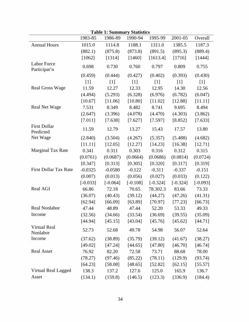
Table 1: Summary Statistics 1983-85 1986-89 1990-94 1995-99 2001-05 Overall

Annual Hours 1015.0 1114.8 1188.1 1311.0 1385.5 1187.3 (882.1) (875.8) (873.8) (891.5) (895.3) (889.4) [1062] [1314] [1460] [1613.4] [1716] [1444]

Labor Force Participat’n

0.698 0.730 0.760 0.797 0.809 0.755

(0.459) (0.444) (0.427) (0.402) (0.393) (0.430) [1] [1] [1] [1] [1] [1]

Real Gross Wage 11.59 12.27 12.33 12.95 14.30 12.56 (4.494) (5.293) (6.328) (6.976) (6.782) (6.047) [10.67] [11.06] [10.80] [11.02] [12.88] [11.11] Real Net Wage 7.531 8.349 8.482 8.741 9.695 8.494 (2.647) (3.396) (4.078) (4.470) (4.303) (3.862) [7.011] [7.638] [7.627] [7.597] [8.852] [7.633] First Dollar Predicted

11.59 12.79 13.27 15.43 17.57 13.80

Net Wage (2.840) (3.504) (4.267) (5.357) (5.488) (4.682) [11.11] [12.05] [12.27] [14.23] [16.38] [12.71] Marginal Tax Rate 0.341 0.311 0.303 0.316 0.312 0.315 (0.0761) (0.0687) (0.0664) (0.0686) (0.0814) (0.0724) [0.347] [0.313] [0.305] [0.320] [0.317] [0.319] First Dollar Tax Rate -0.0325 -0.0580 -0.122 -0.311 -0.337 -0.151 (0.007) (0.013) (0.056) (0.027) (0.033) (0.122) [-0.033] [-0.064] [-0.108] [-0.324] [-0.324] [-0.093] Real AGI 66.86 72.18 70.65 78.302.3 83.66 73.33 (36.07) (40.43) (39.12) (44.27) (47.26) (41.31) [62.94] [66.09] [63.89] [70.97] [77.23] [66.73] Real Nonlabor 47.44 48.89 47.44 52.20 53.33 49.33 Income (32.56) (34.66) (33.54) (36.69) (39.55) (35.09) [44.94] [45.15] [43.04] [45.76] [45.62] [44.71] Virtual Real Nonlabor

52.73 52.68 49.78 54.98 56.07 52.64

Income (37.62) (38.89) (35.79) (39.12) (41.67) (38.27) [49.02] [47.24] [44.65] [47.80] [46.70] [46.74] Real Asset 76.92 82.20 72.58 73.71 88.68 78.00 (78.27) (97.46) (85.22) (78.11) (129.9) (93.74) [64.23] [58.08] [48.65] [52.82] [62.15] [55.57] Virtual Real Lagged 138.3 137.2 127.6 125.0 165.9 136.7 Asset (134.1) (159.8) (146.5) (123.3) (336.9) (184.4)

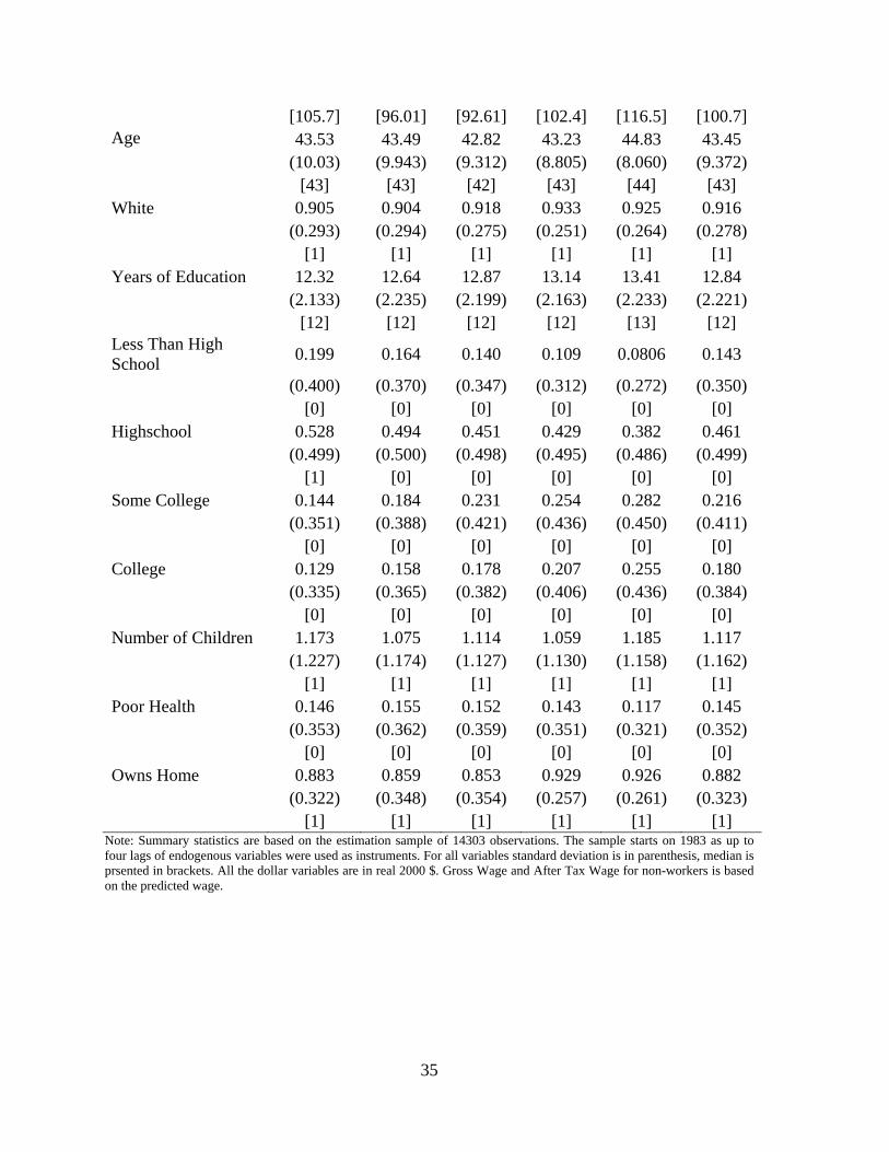
35

[105.7] [96.01] [92.61] [102.4] [116.5] [100.7] Age 43.53 43.49 42.82 43.23 44.83 43.45 (10.03) (9.943) (9.312) (8.805) (8.060) (9.372) [43] [43] [42] [43] [44] [43] White 0.905 0.904 0.918 0.933 0.925 0.916

(0.293) (0.294) (0.275) (0.251) (0.264) (0.278) [1] [1] [1] [1] [1] [1]

Years of Education 12.32 12.64 12.87 13.14 13.41 12.84 (2.133) (2.235) (2.199) (2.163) (2.233) (2.221)

[12] [12] [12] [12] [13] [12] Less Than High School

0.199 0.164 0.140 0.109 0.0806 0.143

(0.400) (0.370) (0.347) (0.312) (0.272) (0.350) [0] [0] [0] [0] [0] [0]

Highschool 0.528 0.494 0.451 0.429 0.382 0.461 (0.499) (0.500) (0.498) (0.495) (0.486) (0.499)

[1] [0] [0] [0] [0] [0] Some College 0.144 0.184 0.231 0.254 0.282 0.216

(0.351) (0.388) (0.421) (0.436) (0.450) (0.411) [0] [0] [0] [0] [0] [0]

College 0.129 0.158 0.178 0.207 0.255 0.180 (0.335) (0.365) (0.382) (0.406) (0.436) (0.384)

[0] [0] [0] [0] [0] [0] Number of Children 1.173 1.075 1.114 1.059 1.185 1.117

(1.227) (1.174) (1.127) (1.130) (1.158) (1.162) [1] [1] [1] [1] [1] [1]

Poor Health 0.146 0.155 0.152 0.143 0.117 0.145 (0.353) (0.362) (0.359) (0.351) (0.321) (0.352)

[0] [0] [0] [0] [0] [0] Owns Home 0.883 0.859 0.853 0.929 0.926 0.882

(0.322) (0.348) (0.354) (0.257) (0.261) (0.323) [1] [1] [1] [1] [1] [1]

Note: Summary statistics are based on the estimation sample of 14303 observations. The sample starts on 1983 as up to four lags of endogenous variables were used as instruments. For all variables standard deviation is in parenthesis, median is prsented in brackets. All the dollar variables are in real 2000 $. Gross Wage and After Tax Wage for non-workers is based on the predicted wage.

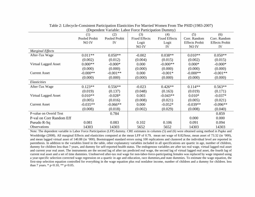
Table 2: Lifecycle-Consistent Participation Elasticities For Married Women From The PSID (1983-2007) (Dependent Variable: Labor Force Participation Dummy)

(1) (2) (3) (4) (5) (6) Pooled Probit

NO IV Pooled Probit

IV Fixed Effects

Logit NO IV

Fixed Effects Logit

IV

Corr. Random Effects Probit

NO IV

Corr. Random Effects Probit

IV Marginal Effects After-Tax Wage 0.011** 0.050** -0.002 0.038** 0.010** 0.050** (0.002) (0.012) (0.004) (0.015) (0.002) (0.015) Virtual Lagged Asset 0.000** -0.000* 0.000 -0.000** 0.000* -0.000* (0.000) (0.000) (0.000) (0.000) (0.000) (0.000) Current Asset -0.000** -0.001** 0.000 -0.001* -0.000** -0.001** (0.000) (0.000) (0.000) (0.000) (0.000) (0.000) Elasticities After-Tax Wage 0.123** 0.556** -0.023 0.426** 0.114** 0.563** (0.019) (0.137) (0.048) (0.163) (0.019) (0.171) Virtual Lagged Asset 0.010** -0.028* 0.003 -0.043** 0.010* -0.037* (0.005) (0.016) (0.008) (0.021) (0.005) (0.021) Current Asset -0.035** -0.066** 0.000 -0.052* -0.039** -0.096** (0.008) (0.018) (0.002) (0.029) (0.008) (0.040) P-value on Overid Test 0.784 0.859 P-val on Corr Random Eff 0.000 0.000 Pseudo R-Sq 0.081 0.083 0.102 0.106 0.091 0.094 Observations 14303 14303 5652 5652 14303 14303 Note: The dependent variable is Labor Force Participation (LFP) dummy. CRE estimates in columns (5) and (6) were obtained using method in Papke and Wooldridge (2008). All marginal Effects and elasticities computed at the mean LFP of 0.79, mean net wage of 8.82/hour, mean asset of 73.32 (in ‘000), and mean lagged virtual asset of 140.88 (in ‘000). Bootstrapped standard errors using 100 replications and clustered at the individual level are reported in parenthesis. In addition to the variables listed in the table, other explanatory variables included in all specifications are quartic in age, number of children, dummy for children less than 7 years, and dummy for self-reported health status. The endogenous variables are after tax real wage, virtual lagged real asset and current year real asset. The instruments are the second lag of after tax predicted real wage, the second lag of virtual lagged real asset, the fourth lag of current real asset and a set of time dummies. Unobserved after-tax real wage for non-labor-force-participating females was replaced by wage imputed using a year-specific selection corrected wage regression on a quartic in age and education, race dummies,and state dummies. To estimate the wage equation, the first-step selection equation controlled for everything in the wage equation plus real nonlabor income, number of children and a dummy for children. less than 7 years. * p<0.10, ** p<0.05.

37

Table 3: Selection-Corrected Lifecycle-Consistent Hours Elasticities for Married Women from the PSID (1983-2007) (Dependent Variable: Annual Hours Of Work)

(1) (2) (3) (4) (5) (6) Pooled

Heckman NO IV

Pooled Heckman

IV

Semiparametric Fixed Effects

NO IV

Semiparametric Fixed Effects

IV

Corr. Random Effects with

Selection NO IV

Corr. Random Effects with

Selection IV

Marginal Effects After-Tax Wage 11.776** 99.107** -8.978 61.031 23.931** 55.202* (3.878) (46.741) (46.978) (53.969) (4.279) (32.300) Virtual Lagged Asset 0.063 0.156 0.188 0.509 0.179** 0.151 (0.063) (0.169) (0.454) (0.731) (0.064) (0.352) Current Asset -0.658** -2.248** 0.303 0.008 -0.688** -2.612** (0.193) (0.694) (0.694) (2.402) (0.136) (0.983) Elasticities After-Tax Wage 0.065** 0.549** -0.050 0.338 0.133** 0.306* (0.021) (0.259) (0.260) (0.299) (0.024) (0.179) Virtual Lagged Asset 0.005 0.013 0.001 0.003 0.015** 0.013 (0.005) (0.014) (0.003) (0.004) (0.005) (0.029) Current Asset -0.028** -0.097** 0.002 0.000 -0.030** -0.112** (0.008) (0.030) (0.004) (0.013) (0.006) (0.042) P-value on Overid Test 0.013 0.990 0.008 P-val on Corr Random Eff 0.000 0.000 R-Sq 0.08 0.07 0.01 0.03 0.10 0.06 Observations 10998 10998 6515 7156 10998 10998

Note: The dependent variable is annual hours of work. Semiparametric Fixed Effects estimates in columns (3) and (4) used method in Kyriazidou (1997). CRE estimates in columns (5) and (6) were obtained using method in Semykina and Wooldridge (2010). All marginal Effects and elasticities computed at the mean hours for labor force participants of 1589, mean net wage of 9.05/hour, mean asset of 70.81 (in ‘000), and mean lagged virtual asset of 141.40 (in ‘000). Bootstrapped standard errors using 100 replications and clustered at the individual level are reported in parenthesis. The endogenous variables are after tax real wage, virtual lagged real asset and current year real asset. The instruments are the second lag of after tax predicted real wage, the second lag of virtual lagged real asset, the fourth lag of current real asset and a set of time dummies. To obtain the inverse mills ratio, the first step reduced form LFP equation was estimated on the instruments, quartic in age, number of children, dummy for children less than 7 years , and dummy for self-reported health status. The exclusion restriction for the second step selection-corrected hours equation was dummy for children less than 7 years. * p<0.10, ** p<0.05

38

Table 4: Lifecycle-Consistent Total Labor Supply Elasticities for Married Women from the PSID (1983-2007) (Dependent Variable: Annual Hours of Work)

(1) (2) (3) (4) (5) (6) Pooled Tobit

NO IV Pooled Tobit

IV Semiparametric Fixed Effects

NO IV

Semiparametric Fixed Effects

IV

Corr. Random Effects Tobit

NO IV

Corr. Random Effects Tobit

IV Marginal Effects After-Tax Wage 34.722** 169.506** -10.302** 69.476** 32.935** 141.465** (3.667) (43.680) (4.462) (22.181) (3.824) (45.184) Virtual Lagged Asset 0.211** -0.277 0.214** -0.403* 0.201** -0.182 (0.085) (0.206) (0.078) (0.236) (0.083) (0.241) Current Asset -1.437** -3.077** -0.167 -1.663** -1.518** -2.480** (0.203) (0.668) (0.154) (0.843) (0.205) (1.038) Elasticities After-Tax Wage 0.245** 1.195** -0.073** 0.490** 0.232** 0.997** (0.026) (0.308) (0.031) (0.156) (0.027) (0.319) Virtual Lagged Asset 0.023** -0.030 0.023** -0.043* 0.022** -0.020 (0.009) (0.022) (0.008) (0.025) (0.009) (0.026) Current Asset -0.083** -0.178** -0.010 -0.096** -0.088** -0.144** (0.012) (0.039) (0.009) (0.049) (0.012) (0.060) P-value on Overid Test 0.756 0.675 P-val on Corr Random Eff 0.000 0.000 Pseudo R-Sq 0.010 0.011 0.012 0.012 Observations 14303 14303 14303 14303 14303 14303 Note: The dependent variable is annual hours of work. Semiparametric Fixed Effects estimates in columns (3) and (4) used method in Honoré (1992). CRE estimates in columns (5) and (6) were obtained using method in Papke and Wooldridge (2008) All marginal Effects and elasticities computed at the mean hours of 1156, mean net wage of 8.82/hour, mean asset of 73.32 (in ‘000), and mean lagged virtual asset of 140.88 (in ‘000). Bootstrapped standard errors using 100 replications and clustered at the individual level are reported in parenthesis. In addition to the variables listed in the table, other explanatory variables included in all specifications are quartic in age, number of children, dummy for children less than 7 years, and dummy for self-reported health status. The endogenous variables are after tax real wage, virtual lagged real asset and current year real asset. The instruments are the second lag of after tax predicted real wage, the second lag of virtual lagged real asset, the fourth lag of current real asset and a set of time dummies. Unobserved after-tax real wage for non-labor-force-participating females was replaced by wage imputed using a year-specific selection corrected wage regression on a quartic in age and education, race dummies,and state dummies. To estimate the wage equation, the first-step selection equation controlled for everything in the wage equation plus real nonlabor income, number of children and a dummy for children less than 7 years. * p<0.10, ** p<0.05

39

Table 5: Sensitivity of Estimated Labor Supply Elasticities to Taxes and Lifecycle-specifications (1) (2) (3) (4) (5) (6) (7) (8) (9) Lifecycle Model With

Nonlinear Taxes Lifecycle Model With

Linear Taxes Static Model With Taxes

Pooled IV Fixed Effects IV

Corr. Random

Effects IV

Pooled IV

Fixed Effects IV

Corr. Random

Effects IV

Pooled IV Fixed Effects

IV

Corr. Random Effects

IV Participation Elasticity After-Tax Wage 0.556** 0.426** 0.563** 0.590** 0.444** 0.531** 0.534** 0.697** 0.457** (0.137) (0.163) (0.171) (0.188) (0.089) (0.160) (0.123) (0.118) (0.146) Lagged Virtual Assets -0.028* -0.043** -0.037* (0.016) (0.021) (0.021) Current Assets -0.066** -0.052* -0.096** (0.018) (0.029) (0.040) Virtual Net Saving -0.004 -0.002** -0.005** (0.003) (0.001) (0.002) Virtual Income -0.187** -0.119** -0.056 (0.030) (0.038) (0.068) Hours Elasticity After-Tax Wage 0.549** 0.338 0.306* 0.523* 0.147 0.290** 0.579** 0.157 0.127 (0.259) (0.299) (0.179) (0.289) (0.239) (0.147) (0.235) (0.256) (0.196) Lagged Virtual Assets 0.013 0.003 0.013 (0.014) (0.004) (0.029) Current Assets -0.097** 0.000 -0.112** (0.030) (0.013) (0.042) Virtual Net Saving 0.002 0.004 -0.002 (0.004) (0.007) (0.005) Virtual Income -0.153** -0.008 -0.135* (0.054) (0.035) (0.072) P-value Overid Test 0.784 0.859 0.705 0.729 0.186 0.213 Pseudo R-Sq 0.083 0.106 0.094 0.079 0.102 0.088 0.095 0.102 0.111

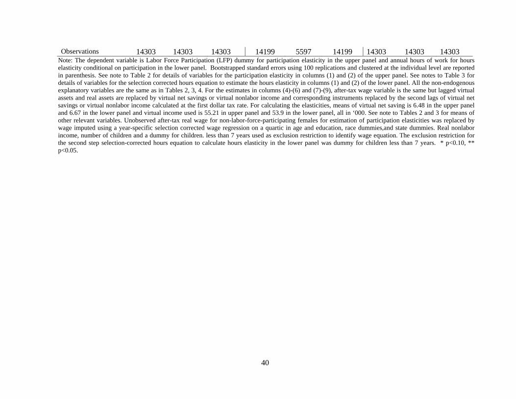
40

Observations 14303 14303 14303 14199 5597 14199 14303 14303 14303 Note: The dependent variable is Labor Force Participation (LFP) dummy for participation elasticity in the upper panel and annual hours of work for hours elasticity conditional on participation in the lower panel. Bootstrapped standard errors using 100 replications and clustered at the individual level are reported in parenthesis. See note to Table 2 for details of variables for the participation elasticity in columns (1) and (2) of the upper panel. See notes to Table 3 for details of variables for the selection corrected hours equation to estimate the hours elasticity in columns (1) and (2) of the lower panel. All the non-endogenous explanatory variables are the same as in Tables 2, 3, 4. For the estimates in columns (4)-(6) and (7)-(9), after-tax wage variable is the same but lagged virtual assets and real assets are replaced by virtual net savings or virtual nonlabor income and corresponding instruments replaced by the second lags of virtual net savings or virtual nonlabor income calculated at the first dollar tax rate. For calculating the elasticities, means of virtual net saving is 6.48 in the upper panel and 6.67 in the lower panel and virtual income used is 55.21 in upper panel and 53.9 in the lower panel, all in ‘000. See note to Tables 2 and 3 for means of other relevant variables. Unobserved after-tax real wage for non-labor-force-participating females for estimation of participation elasticities was replaced by wage imputed using a year-specific selection corrected wage regression on a quartic in age and education, race dummies,and state dummies. Real nonlabor income, number of children and a dummy for children. less than 7 years used as exclusion restriction to identify wage equation. The exclusion restriction for the second step selection-corrected hours equation to calculate hours elasticity in the lower panel was dummy for children less than 7 years. * p<0.10, ** p<0.05.

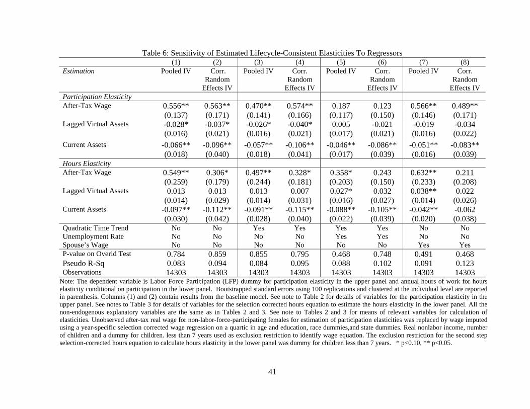
41

Table 6: Sensitivity of Estimated Lifecycle-Consistent Elasticities To Regressors (1) (2) (3) (4) (5) (6) (7) (8) Estimation Pooled IV Corr.

Random Effects IV

Pooled IV Corr. Random

Effects IV

Pooled IV Corr. Random

Effects IV

Pooled IV Corr. Random

Effects IV Participation Elasticity After-Tax Wage 0.556** 0.563** 0.470** 0.574** 0.187 0.123 0.566** 0.489** (0.137) (0.171) (0.141) (0.166) (0.117) (0.150) (0.146) (0.171) Lagged Virtual Assets -0.028* -0.037* -0.026* -0.040* 0.005 -0.021 -0.019 -0.034 (0.016) (0.021) (0.016) (0.021) (0.017) (0.021) (0.016) (0.022) Current Assets -0.066** -0.096** -0.057** -0.106** -0.046** -0.086** -0.051** -0.083** (0.018) (0.040) (0.018) (0.041) (0.017) (0.039) (0.016) (0.039) Hours Elasticity After-Tax Wage 0.549** 0.306* 0.497** 0.328* 0.358* 0.243 0.632** 0.211 (0.259) (0.179) (0.244) (0.181) (0.203) (0.150) (0.233) (0.208) Lagged Virtual Assets 0.013 0.013 0.013 0.007 0.027* 0.032 0.038** 0.022 (0.014) (0.029) (0.014) (0.031) (0.016) (0.027) (0.014) (0.026) Current Assets -0.097** -0.112** -0.091** -0.115** -0.088** -0.105** -0.042** -0.062 (0.030) (0.042) (0.028) (0.040) (0.022) (0.039) (0.020) (0.038) Quadratic Time Trend No No Yes Yes Yes Yes No No Unemployment Rate No No No No Yes Yes No No Spouse’s Wage No No No No No No Yes Yes P-value on Overid Test 0.784 0.859 0.855 0.795 0.468 0.748 0.491 0.468 Pseudo R-Sq 0.083 0.094 0.084 0.095 0.088 0.102 0.091 0.123 Observations 14303 14303 14303 14303 14303 14303 14303 14303

Note: The dependent variable is Labor Force Participation (LFP) dummy for participation elasticity in the upper panel and annual hours of work for hours elasticity conditional on participation in the lower panel. Bootstrapped standard errors using 100 replications and clustered at the individual level are reported in parenthesis. Columns (1) and (2) contain results from the baseline model. See note to Table 2 for details of variables for the participation elasticity in the upper panel. See notes to Table 3 for details of variables for the selection corrected hours equation to estimate the hours elasticity in the lower panel. All the non-endogenous explanatory variables are the same as in Tables 2 and 3. See note to Tables 2 and 3 for means of relevant variables for calculation of elasticities. Unobserved after-tax real wage for non-labor-force-participating females for estimation of participation elasticities was replaced by wage imputed using a year-specific selection corrected wage regression on a quartic in age and education, race dummies,and state dummies. Real nonlabor income, number of children and a dummy for children. less than 7 years used as exclusion restriction to identify wage equation. The exclusion restriction for the second step selection-corrected hours equation to calculate hours elasticity in the lower panel was dummy for children less than 7 years. * p<0.10, ** p<0.05.

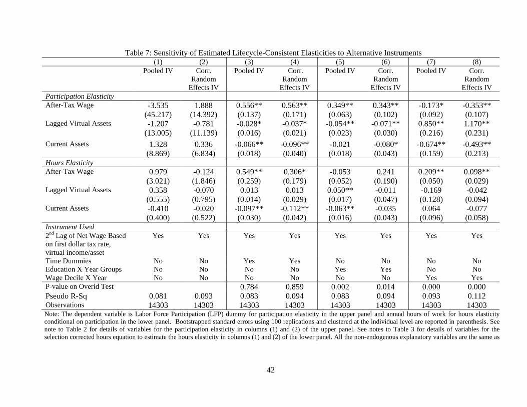
42

Table 7: Sensitivity of Estimated Lifecycle-Consistent Elasticities to Alternative Instruments (1) (2) (3) (4) (5) (6) (7) (8) Pooled IV Corr.

Random Effects IV

Pooled IV Corr. Random

Effects IV

Pooled IV Corr. Random

Effects IV

Pooled IV Corr. Random

Effects IV Participation Elasticity After-Tax Wage -3.535 1.888 0.556** 0.563** 0.349** 0.343** -0.173* -0.353** (45.217) (14.392) (0.137) (0.171) (0.063) (0.102) (0.092) (0.107) Lagged Virtual Assets -1.207 -0.781 -0.028* -0.037* -0.054** -0.071** 0.850** 1.170** (13.005) (11.139) (0.016) (0.021) (0.023) (0.030) (0.216) (0.231) Current Assets 1.328 0.336 -0.066** -0.096** -0.021 -0.080* -0.674** -0.493** (8.869) (6.834) (0.018) (0.040) (0.018) (0.043) (0.159) (0.213) Hours Elasticity After-Tax Wage 0.979 -0.124 0.549** 0.306* -0.053 0.241 0.209** 0.098** (3.021) (1.846) (0.259) (0.179) (0.052) (0.190) (0.050) (0.029) Lagged Virtual Assets 0.358 -0.070 0.013 0.013 0.050** -0.011 -0.169 -0.042 (0.555) (0.795) (0.014) (0.029) (0.017) (0.047) (0.128) (0.094) Current Assets -0.410 -0.020 -0.097** -0.112** -0.063** -0.035 0.064 -0.077 (0.400) (0.522) (0.030) (0.042) (0.016) (0.043) (0.096) (0.058) Instrument Used 2nd Lag of Net Wage Based on first dollar tax rate, virtual income/asset

Yes Yes Yes Yes Yes Yes Yes Yes

Time Dummies No No Yes Yes No No No No Education X Year Groups No No No No Yes Yes No No Wage Decile X Year No No No No No No Yes Yes P-value on Overid Test 0.784 0.859 0.002 0.014 0.000 0.000 Pseudo R-Sq 0.081 0.093 0.083 0.094 0.083 0.094 0.093 0.112 Observations 14303 14303 14303 14303 14303 14303 14303 14303 Note: The dependent variable is Labor Force Participation (LFP) dummy for participation elasticity in the upper panel and annual hours of work for hours elasticity conditional on participation in the lower panel. Bootstrapped standard errors using 100 replications and clustered at the individual level are reported in parenthesis. See note to Table 2 for details of variables for the participation elasticity in columns (1) and (2) of the upper panel. See notes to Table 3 for details of variables for the selection corrected hours equation to estimate the hours elasticity in columns (1) and (2) of the lower panel. All the non-endogenous explanatory variables are the same as

43

in Tables 2 and 3. See note to Tables 2 and 3 for means of relevant variables for calculation of elasticities. Unobserved after-tax real wage for non-labor-force-participating females for estimation of participation elasticities was replaced by wage imputed using a year-specific selection corrected wage regression on a quartic in age and education, race dummies,and state dummies. Real nonlabor income, number of children and a dummy for children. less than 7 years used as exclusion restriction to identify wage equation. The exclusion restriction for the second step selection-corrected hours equation to calculate hours elasticity in the lower panel was dummy for children less than 7 years. * p<0.10, ** p<0.05.

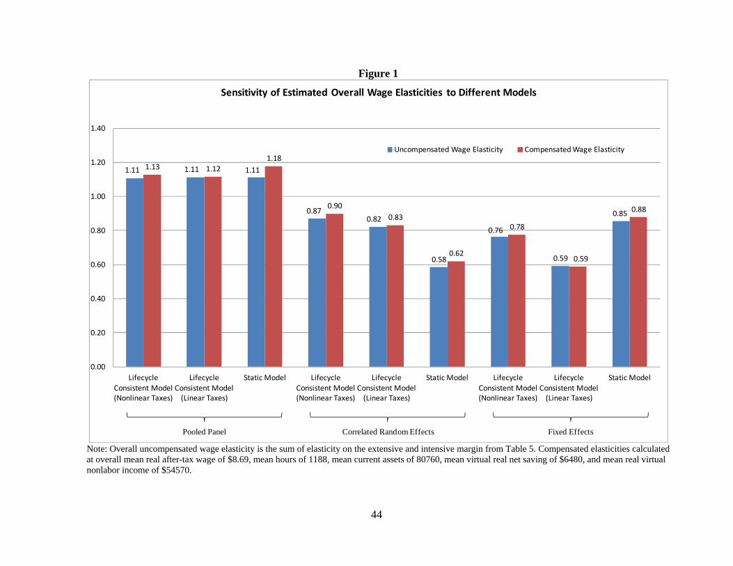
44

Figure 1

Note: Overall uncompensated wage elasticity is the sum of elasticity on the extensive and intensive margin from Table 5. Compensated elasticities calculated at overall mean real after-tax wage of $8.69, mean hours of 1188, mean current assets of 80760, mean virtual real net saving of $6480, and mean real virtual nonlabor income of $54570.

1.11 1.11 1.11

0.870.82

0.58

0.76

0.59

0.85

1.13 1.121.18

0.900.83

0.62

0.78

0.59

0.88

0.00

0.20

0.40

0.60

0.80

1.00

1.20

1.40

Lifecycle Consistent Model (Nonlinear Taxes)

Lifecycle Consistent Model (Linear Taxes)

Static Model Lifecycle Consistent Model (Nonlinear Taxes)

Lifecycle Consistent Model (Linear Taxes)

Static Model Lifecycle Consistent Model (Nonlinear Taxes)

Lifecycle Consistent Model (Linear Taxes)

Static Model

Sensitivity of Estimated Overall Wage Elasticities  to Different Models

Uncompensated Wage Elasticity Compensated Wage Elasticity

Pooled Panel Correlated Random Effects Fixed Effects

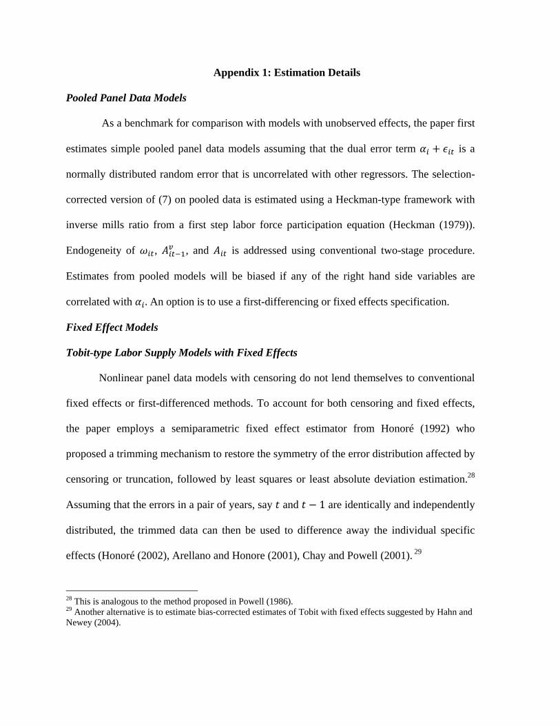
Appendix 1: Estimation Details

Pooled Panel Data Models

As a benchmark for comparison with models with unobserved effects, the paper first

estimates simple pooled panel data models assuming that the dual error term is a

normally distributed random error that is uncorrelated with other regressors. The selection-

corrected version of (7) on pooled data is estimated using a Heckman-type framework with

inverse mills ratio from a first step labor force participation equation (Heckman (1979)).

Endogeneity of , , and is addressed using conventional two-stage procedure.

Estimates from pooled models will be biased if any of the right hand side variables are

correlated with . An option is to use a first-differencing or fixed effects specification.

Fixed Effect Models

Tobit-type Labor Supply Models with Fixed Effects

Nonlinear panel data models with censoring do not lend themselves to conventional

fixed effects or first-differenced methods. To account for both censoring and fixed effects,

the paper employs a semiparametric fixed effect estimator from Honoré (1992) who

proposed a trimming mechanism to restore the symmetry of the error distribution affected by

censoring or truncation, followed by least squares or least absolute deviation estimation.28

Assuming that the errors in a pair of years, say and 1 are identically and independently

distributed, the trimmed data can then be used to difference away the individual specific

effects (Honoré (2002), Arellano and Honore (2001), Chay and Powell (2001). 29

28 This is analogous to the method proposed in Powell (1986). 29 Another alternative is to estimate bias-corrected estimates of Tobit with fixed effects suggested by Hahn and Newey (2004).

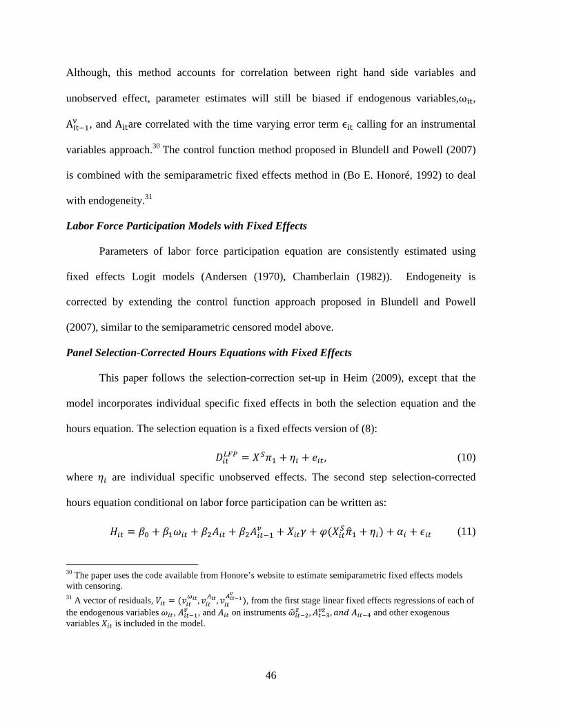
46

Although, this method accounts for correlation between right hand side variables and

unobserved effect, parameter estimates will still be biased if endogenous variables,ω ,

A , and A are correlated with the time varying error term calling for an instrumental

variables approach.30 The control function method proposed in Blundell and Powell (2007)

is combined with the semiparametric fixed effects method in (Bo E. Honoré, 1992) to deal

with endogeneity.31

Labor Force Participation Models with Fixed Effects

Parameters of labor force participation equation are consistently estimated using

fixed effects Logit models (Andersen (1970), Chamberlain (1982)). Endogeneity is

corrected by extending the control function approach proposed in Blundell and Powell

(2007), similar to the semiparametric censored model above.

Panel Selection-Corrected Hours Equations with Fixed Effects

This paper follows the selection-correction set-up in Heim (2009), except that the

model incorporates individual specific fixed effects in both the selection equation and the

hours equation. The selection equation is a fixed effects version of (8):

, (10)

where are individual specific unobserved effects. The second step selection-corrected

hours equation conditional on labor force participation can be written as:

(11)

30 The paper uses the code available from Honore’s website to estimate semiparametric fixed effects models with censoring. 31 A vector of residuals, , , , from the first stage linear fixed effects regressions of each of the endogenous variables , , and on instruments , , and other exogenous variables is included in the model.

47

where is the inverse mills ratio obtained from the first step. Although,

individual specific effects can be eliminated by differencing, enters the equation

nonlinearly through the inverse mills ratio and cannot be eliminated by differencing.

The paper applies a semiparametric selection correction method proposed in

Kyriazidou (1997). First, parameters of the selection equation (10) are estimated using a

consistent estimator e.g. fixed effect Logit. Then for any two time periods, 1 and in

which the female participates in the labor force, if Δ then first differencing

(11) would difference away not only but also and . Because has both

continuous and discrete elements, Δ is unlikely to equal zero. However, estimation can

be restricted to observations for which, Δ is small. Better still, using all observations

and estimating the following weighted least squares equation for labor force participants

with weights going to zero if |Δ | increases, yields consistent estimates:

ξΔ ξΔ ξΔ ξΔ ξΔ ξΔ , (12)

where ξ K is a kernel weight function with h , the bandwidth.

Endogeneity in (12) is dealt with following a straightforward application of the two-

stage procedure adopted in Charlier et al. (2001) with Δ , Δ , Δ used as

instruments.

Semiparametric fixed effects methods solve the problem of correlated unobserved

heterogeneity, heteroscedasticity, and nonnormality of the error distributions. However, an

important limitation is that average partial effects and therefore, elasticities are, in general,

not identified, as the unobserved effects are not estimated Wooldridge (2010). Papke and

48

Wooldridge (2008) and Wooldridge (2009) showed that estimating average partial effects is

feasible in a correlated random effects framework.

Correlated Random Effects (CRE) Tobit and Probit Models

Letting be a linear function of time means of , , , , so that

and substituting in (7) yields the CRE

specification,

, (13)

Assuming strict exogeneity and normality of the composite error term (13) is

estimated using a Probit or a Tobit.32

Control function approach proposed in Papke and Wooldridge (2008) and

Wooldridge (2009) is used to account for endogeneity. Letting , represent the exogenous

variables in the model and , the instruments , , , so that

, represents the vector of all exogenous variables and instruments. Also let

, , be the time means of all exogenous variables, included exogenous variables, and

excluded instruments, respectively. The first stage in (13) consists of regressing each

endogenous variable, , , , on and and getting the vector of residuals

32Typically such CRE specifications are applicable only for balanced panels. However, following Wooldridge (2009), CRE can be adapted for unbalanced panels by assuming that in addition to strict exogeneity of covariates selection into the panel is also strictly exogenous i.e. dropping out of the panel is not systematically correlated with .

49

, , . In the second stage, hours or labor force participation is regressed on

, , , , , , , .33

Correlated Random Effect Models with Selection Correction

Semykina and Wooldridge (2010) proposed a parametric method to account for

correlated individual effects in the selection equation (10) as well as the main equation (11),

which combines the typical Heckman-type selectivity correction with correlated random

effects models similar in spirit to (13). In the specification without endogeneity, in the first

step, year-specific inverse mills ratio, are obtained by running a Probit of on

and for each . In the second step, the specification in (13) is augmented with

∑ .

To account for endogeneity, Semykina and Wooldridge (2010) proposed 2SLS

estimation similar in spirit to Papke and Wooldridge (2008) and Wooldridge (2009). In the

first step a Heckman-type selection equation is estimated by running a reduced form Probit

of labor force participation on and an exclusion restriction 7 for each year

separately and the year-specific inverse mills ratio for each labor force participant, ,

saved. In the second step hours is regressed on , , , , , , in a 2sls

framework treating , , as endogenous.

33 Note that time means of endogenous variables are not included in the second stage CRE specification. Instead the time means of exogenous variables and instruments are included.