Life Cycle Assessment of Asphalt Pavements

including the Feedstock Energy and Asphalt

Additives

Licentiate Thesis

Ali Azhar Butt

Division of Highway and Railway Engineering

Department of Transport Science

School of Architecture and the Built Environment

KTH, Royal Institute of Technology

SE-100 44 Stockholm

SWEDEN

October 2012

© Ali Azhar Butt

TRITA-TSC-LIC 12-008

ISBN 978-91-85539-96-3

i

Abstract:

Roads are assets to the society and an integral component in the development of a nation’s

infrastructure. To build and maintain roads; considerable amounts of materials are required

which consume quite an amount of electrical and thermal energy for production, processing

and laying. The resources (materials and the sources of energy) should be utilized efficiently

to avoid wastes and higher costs in terms of the currency and the environment.

In order to enable quantification of the potential environmental impacts due to the

construction, maintenance and disposal of roads, an open life cycle assessment (LCA)

framework for asphalt pavements was developed. Emphasis was given on the calculation

and allocation of energy used for the binder and the additives. Asphalt mixtures properties

can be enhanced against rutting and cracking by modifying the binder with additives. Even

though the immediate benefits of using additives such as polymers and waxes to modify the

binder properties are rather well documented, the effects of such modification over the

lifetime of a road are seldom considered. A method for calculating energy allocation in

additives was suggested. The different choices regarding both the framework design and the

case specific system boundaries were done in cooperation with the asphalt industry and the

construction companies in order to increase the relevance and the quality of the assessment.

Case-studies were performed to demonstrate the use of the LCA framework. The suggested

LCA framework was demonstrated in a limited case study (A) of a typical Swedish asphalt

pavement. Sensitivity analyses were also done to show the effect and the importance of the

transport distances and the use of efficiently produced electricity mix. It was concluded that

the asphalt production and materials transportation were the two most energy consuming

processes that also emit the most GreenHouse Gases (GHG’s). The GHG’s, however, are

largely depending on the fuel type and the electricity mix. It was also concluded that when

progressing from LCA to its corresponding life cycle cost (LCC) the feedstock energy of the

binder becomes highly relevant as the cost of the binder will be reflected in its alternative

value as fuel. LCA studies can help to develop the long term perspective, linking

performance to minimizing the overall energy consumption, use of resources and emissions.

To demonstrate this, the newly developed open LCA framework was used for an

unmodified and polymer modified asphalt pavement (Case study B). It was shown how

polymer modification for improved performance affects the energy consumption and

emissions during the life cycle of a road. From the case study (C) it was concluded that using

bitumen with self-healing capacity can lead to a significant reduction in the GHG emissions

and the energy usage. Furthermore, it was concluded that better understanding of the

binder would lead to better optimized pavement design and thereby to reduced energy

consumption and emissions. Production energy limits for the wax and polymer were

determined which can assist the additives manufacturers to modify their production

procedures and help road authorities in setting ‘green’ limits to get a real benefit from the

additives over the lifetime of a road.

Keywords: Life Cycle Assessment; feedstock energy; asphalt binder additives; mass-energy

flows; bitumen healing; wax; polymer

ii

iii

Preface

The work presented in this licentiate thesis has been carried out at KTH, Royal Institute of

Technology, at the division of Highway and Railway Engineering.

FORMAS and Akzo Nobel are greatly appreciated for financing this study.

I would specially like to thank and give my high regards to my supervisor, Professor Björn

Birgission and co-supervisor, Dr. Susanna Toller, for their guidance during this process.

What I have achieved, wouldn’t have been possible without their time and supervision. I am

deeply indebted to Prof. Niki Kringos whose suggestions and encouragement helped me do

even more than I planned for.

I am very grateful to Mr. Måns Collin for sharing his expertise with us in the development

and improvement of this work. I will also like to acknowledge the discussions and expert

advices in regular Friday meetings with Dr. Jonas Ekblad, Dr. Per Redelius and other

industry members from Trafikverket, Skanska, Nynas, NCC and Akzo Nobel. I would also

like to thank all the members of GESP project.

Special thanks to my mom, grandma, sister and brother for always being with me.

In the end, I want to thank my wife, Amna Ali Butt, for her love and belief in me, and my

family in Pakistan and abroad for their moral support.

I could go on and on thanking a lot more people but, honestly, thanks a lot everyone for your

love and support.

Ali Azhar Butt

Stockholm, Oct’12

iv

v

Dedication

Allhamdullilah……

In the name of Allah, The most Gracious, The most Merciful.

“O my Lord! Open for me my chest (grant me self-confidence, contentment and boldness).

And ease my task for me; And loose the knot from my tongue. That they understand my

speech.” (Surah Taha, verses 25-28)

I would like to dedicate my work to my parents specially my dad, Azhar Mahmood Butt

(late), who will be proud of me somewhere in the other world.

I surely love and miss you dad!!!

vi

vii

Publications

This Licentiate thesis is based on the following publications:

Journal:

I. Butt, A.A., Mirzadeh, I., Toller, S. and Birgisson, B. (2012), “Life Cycle Assessment Framework for asphalt pavements; Methods to calculate and allocate energy of binder and additives”, International Journal of Pavement Engineering, DOI:10.1080/10298436.2012.718348.

II. Butt, A.A., Birgisson, B. and Kringos, N. (2013), “Considering the benefits of asphalt

modification using a new technical LCA framework”, submitted for a special edition of International Journal of Road Materials and Pavement Design in 5th EATA conference, 3-5 June, Braunschweig, Germany.

Conference: III. Butt, A.A., Birgisson, B. and Kringos, N. (2012), “Optimizing the Highway Lifetime

by Improving the Self Healing Capacity of Asphalt”, Procedia - Social and Behavioral Sciences, Fourth Transport Research Arena, Vol. 48, 23-26 April, Athens, Greece, p. 2190-2200.

Other relevant publications:

i. Butt, A.A., Tasdemir, Y. and Edwards, Y. (2009), “Environmental friendly wax modified mastic asphalt”, II International Conference on Environmentally Friendly Roads, ENVIROAD, 15-16 Oct, Warsaw, Poland.

ii. Edwards, Y., Tasdemir, Y. and Butt, A.A. (2010), “Energy saving and environmental

friendly wax concept for polymer modified mastic asphalt”, Materials and Structures, Vol. 43, supplement 1, p. 123-131.

iii. Butt, A.A., Jelagin, D., Tasdemir, Y. and Birgisson, B. (2010), “The Effect of Wax

Modification on the Performance of Mastic Asphalt”, International Journal of Pavement Research and Technology, Vol. 3, No. 2, p. 86-95.

iv. Mirzadeh, I., Butt, A.A., Toller, S. and Birgisson, B. (2012), “Life Cycle Cost Analysis

Based on Time and Energy Entities for Asphalt Pavements”, under review in International Journal of Pavement Engineering.

v. Mirzadeh, I., Butt, A.A., Toller, S. and Birgisson, B. (2012), “A Life Cycle Cost

Approach based on the Calibrated Mechanistic Asphalt Pavement Design Model”, European Pavement and Asset Management Conference, EPAM, 5–7 Sep, Malmö, Sweden.

viii

vi. Butt, A.A., Mirzadeh, I., Toller, S. and Birgisson, B. (2012), “Bitumen Feedstock Energy and Electricity production in Pavement LCA”, ISAP 2012 International Symposium on Heavy Duty Asphalt Pavements and Bridge Deck Pavements, 23-25 May, Nanjing, China.

vii. Butt, A.A., Jelagin, D., Birgisson, B. and Kringos, N. (2012), “Using Life Cycle

Assessment to Optimize Pavement Crack-Mitigation”, Scarpas et al. (Eds.), 7th RILEM International Conference on Cracking in Pavements, Vol. 1, 20-22 June, Delft, Netherlands, p. 299-306.

ix

x

Contents

1.0 Introduction ………………………………………………………………………… 1

1.1 Research Aims …………………………………………………………………..…… 2

1.2 Thesis Outline …………………………………………………………………..…… 3

Section 1

2.0 Description of LCA framework (Paper 1) .…………………………………… 4

2.1 System Boundaries ……..…………………….………………………………..…… 4

2.2 Feedstock Energy Calculation ..……………………………………….…...…..…… 5

2.3 Method to calculate Mass-Energy flows …..…………………………………..…… 7

Section 2

3.0 Case studies ………………………….…………………………………………… 9

3.1 Case study A (Paper I) ………………………….……………………………..…… 9

3.2 Case study B (Paper II) …………………….………...………………………..…… 15

3.3 Case study C (Paper II and Paper III) ….…….……….………………………..…… 19

4.0 Conclusions ...……………………………..……………………………….……… 23

References ….………………………………………………………….………….…… 24

xi

1

1.0 Introduction

Roads are assets to the society and an integral component in the development of a

nation’s infrastructure. Sweden has a road network consisting of streets, state and

municipal roads, and private roads which sums up to be about 0.6 million km,

according to Swedish National Road Administration. To build and maintain roads;

considerable amounts of materials including bitumen, aggregates and additives are

required which consume quite an amount of electrical and thermal energy for

production, processing and laying. All these materials and the source of energies are

the resources which are part of the nature. These resources shouldn’t be wasted rather

utilized efficiently to avoid wastes and higher costs in terms of currency and the

environment. Hence, environmental tools are required which can help to determine

and improve the efficient use of such resources.

Life cycle thinking is becoming popular in different fields of research as it is being

recognized that resource depletion and the emissions of different potentially harmful

substances are often a result from the activities in different life cycle stages of a

product´s life. Life Cycle Assessment (LCA) is a versatile tool to investigate the

environmental aspect of a product, a service, a process or an activity by identifying and

quantifying related input and output flows utilized by the system and its delivered

functional output in a life cycle perspective (Baumann et al., 2003). Ideally, it includes

all the processes associated to a product from its ‘cradle-raw material extraction’ to its

‘grave-disposal’. LCA studies can help to determine and minimize the energy

consumption, use of resources and emissions to the environment by giving a better

understanding of the systems. LCAs can also purpose different alternatives for

different phases of a life cycle of the system if we have different design alternatives.

Unfortunately, LCA has not yet been adopted by the industry or the road authorities as

part of the procurement and material selection procedure. This could partly be

explained by the lack of a technical tool that accurately represents all the aspects of the

pavement sector and is able to make close predictions of the in-time pavement

response. This system should be transparent and black boxes should be avoided in the

system.

The potential energy embedded in the resource which is not used as energy source

may be referred to as feedstock energy. Bitumen has a high energy content of 40.2

MJ/kg (Garg et al., 2006) but using bitumen as a fuel results in very high emissions

(Faber, 2002; Herold, 2003) and high energy costs. Aggregate on the other hand is

considered to have no feedstock energy. It has also been reported in number of

previous studies that bitumen has a low expended energy (energy used throughout the

production of a material) of approximately 0.4 to 6 MJ/kg (Zapata et al., 2005). There

are authors who include the feedstock energy of the bitumen but the procedure to

calculate it and the theories behind the decision to include it are seldom explicitly

described. So far the source being referred regarding the feedstock energy of the

bitumen is Garg et al. (2006) and (VTT). A general approach to calculate the feedstock

energy in bitumen seems to be missing.

2

The pros and cons of using polymers and waxes to modify the binder properties are

well documented. The long-term effect of this modification over the entire life time of

the pavement is, however, very seldom considered. In fact, it is not a common practice

to report the energy consumption and emissions for the production of the additives

used in the asphalt industry. Therefore to date, very little data is available for the

production phase of the additives, causing a gap in knowledge of the long-term benefit

from the additives from a life cycle perspective. Considering the importance of such

information, a mass-energy flow framework is needed which is able to calculate the

energy consumption and emissions during the production phase of any material based

on the electricity and fuel usage.

1.1 Research Aims

The objective of this study is to enable the improvements of the asphalt pavement

LCAs by describing methods to consider feedstock energies and the asphalt additives.

The work focuses on asphalt pavement and not the whole road network. A general

framework for LCA of the asphalt pavement was suggested and the methods to

calculate the feedstock energy, and quantify the mass and energy flows of the additives

like waxes and polymers, were developed. The use of the LCA framework and

developed calculation methods was demonstrated in three case studies;

The first case study (A) demonstrates the use of LCA framework for a typical

Swedish asphalt pavement followed by two sensitivity analysis (SA).

o The first SA demonstrates how the transportation distances affect the

overall LCA results.

o The second SA considers the importance of efficient electricity production

and its use.

The second case study (B) focuses on the polymer modification for increased crack

resistance.

The third case study (C) focuses on the self-healing capability of bitumen and the

use of Montan wax.

In addition to enable improved LCAs of pavements, a goal was also to increase the

knowledge on the long-term benefits of asphalt modification by including the energy

and emissions that are associated with their production, and calculating the limits for

the production energies of the additives. These limits can assist the manufacturers to

modify their production procedures and help road-authorities in setting the ‘green’

limits.

3

1.2 Thesis Outline

The thesis has been divided into two sections. The first section describes the LCA

framework for the asphalt pavements. It also suggests a method to estimate feedstock

energy of bitumen and a method to allocate energy in a production phase of the

additives (Paper I). The second section consists of three case studies which show the

broad spectra in which the LCA framework could be used followed by SA (Paper I,

Paper II, Paper III).

4

SECTION 1

2.0 Description of Life Cycle Assessment Framework (Paper I)

The life cycle of a road can be divided into several stages; Extraction of the raw

materials, processing the construction materials, transportation, construction,

operation, maintenance, demolition, recycling and waste treatment. Several researchers

are studying the effects on the environment due to construction, maintenance and

disposal of roads (Birgisdóttir, 2005; Huang et al., 2009; Santero et al., 2010a; 2010b;

Stripple, 2001; Zhang et al., 2008;). Such research enables effective measures to be

identified to reduce the resource use and the environmental loads from the roads, for

example by suggesting changes in the technical procedure or the choice of materials.

There are number of softwares and models developed like Federal Highway

Administration’s (FHWA) RealCost, Caltrans’ Cal B/C and FHWA’s IMPACTS but

most look at the life cycle cost (LCC) analysis or neglect the pavements life cycle

perspective (Santero et al., 2010a). On the other hand, several previous LCA´s of roads

have mostly been focused on comparing asphalt and concrete pavements (Santero et

al., 2010a; 2010b).

In this thesis, construction, maintenance and end of life of a flexible pavement (asphalt

road) were considered for the development of the LCA framework. The functional unit

defines the function of the system and for this study; it includes the length, lane width,

nominal design life and residual material at the end of life of the pavement. The use

phase is however important to consider at the network level when decisions of

constructing a road, bridge or a tunnel are being made. On the other hand, if the fuel

usage and emissions from the traffic are included in a life cycle study at a project level,

it will over shadow all the other phases in a road’s life cycle. The LCA framework

developed in this study focuses on a project level, therefore the use phase was not

considered. Material transport, construction and maintenance equipment, and

machinery are present at each unit process in the road system and each unit process is

based on the design considerations.

2.1 System Boundaries

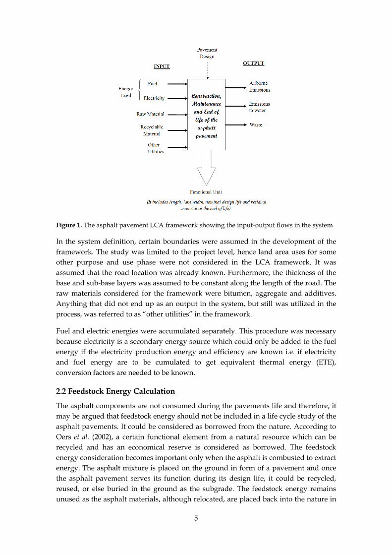
Figure 1 shows the LCA framework for the asphalt pavement. For the development of

the framework, use of the materials was taken as the starting point and end of life of

the pavement to be the end point. The input includes the resources and utilities

whereas the output is the environmental impacts as shown in Figure 1. The energy

consumption and emissions produced in the asphalt production and handling of the

asphalt mixtures and their components were considered.

5

Figure 1. The asphalt pavement LCA framework showing the input-output flows in the system

In the system definition, certain boundaries were assumed in the development of the

framework. The study was limited to the project level, hence land area uses for some

other purpose and use phase were not considered in the LCA framework. It was

assumed that the road location was already known. Furthermore, the thickness of the

base and sub-base layers was assumed to be constant along the length of the road. The

raw materials considered for the framework were bitumen, aggregate and additives.

Anything that did not end up as an output in the system, but still was utilized in the

process, was referred to as “other utilities” in the framework.

Fuel and electric energies were accumulated separately. This procedure was necessary

because electricity is a secondary energy source which could only be added to the fuel

energy if the electricity production energy and efficiency are known i.e. if electricity

and fuel energy are to be cumulated to get equivalent thermal energy (ETE),

conversion factors are needed to be known.

2.2 Feedstock Energy Calculation

The asphalt components are not consumed during the pavements life and therefore, it

may be argued that feedstock energy should not be included in a life cycle study of the

asphalt pavements. It could be considered as borrowed from the nature. According to

Oers et al. (2002), a certain functional element from a natural resource which can be

recycled and has an economical reserve is considered as borrowed. The feedstock

energy consideration becomes important only when the asphalt is combusted to extract

energy. The asphalt mixture is placed on the ground in form of a pavement and once

the asphalt pavement serves its function during its design life, it could be recycled,

reused, or else buried in the ground as the subgrade. The feedstock energy remains

unused as the asphalt materials, although relocated, are placed back into the nature in

6

form of the asphalt mixture. When progressing from a LCA to its corresponding LCC,

however the feedstock energy contents of the binder becomes highly relevant as the

cost of the binder will be reflected in its alternative value as fuel. Therefore, it may be

argued that the energy used within the asphalt materials should be reported although

it is not consumed. What is missing in the literature is the method to calculate the

feedstock energy in the asphalt pavements.

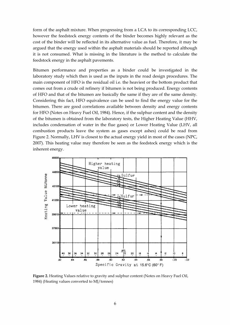
Bitumen performance and properties as a binder could be investigated in the

laboratory study which then is used as the inputs in the road design procedures. The

main component of HFO is the residual oil i.e. the heaviest or the bottom product that

comes out from a crude oil refinery if bitumen is not being produced. Energy contents

of HFO and that of the bitumen are basically the same if they are of the same density.

Considering this fact, HFO equivalence can be used to find the energy value for the

bitumen. There are good correlations available between density and energy contents

for HFO (Notes on Heavy Fuel Oil, 1984). Hence, if the sulphur content and the density

of the bitumen is obtained from the laboratory tests, the Higher Heating Value (HHV,

includes condensation of water in the flue gases) or Lower Heating Value (LHV, all

combustion products leave the system as gases except ashes) could be read from

Figure 2. Normally, LHV is closest to the actual energy yield in most of the cases (NPC,

2007). This heating value may therefore be seen as the feedstock energy which is the

inherent energy.

Figure 2. Heating Values relative to gravity and sulphur content (Notes on Heavy Fuel Oil,

1984) (Heating values converted to MJ/tonnes)

7

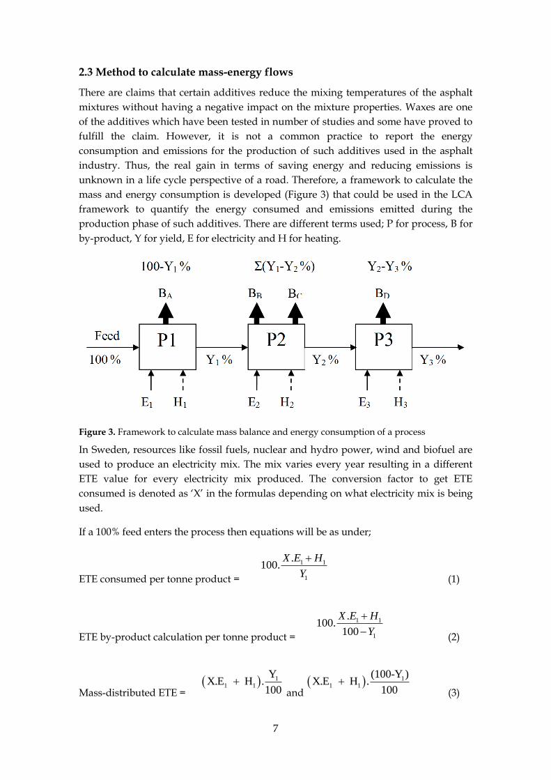
2.3 Method to calculate mass-energy flows

There are claims that certain additives reduce the mixing temperatures of the asphalt

mixtures without having a negative impact on the mixture properties. Waxes are one

of the additives which have been tested in number of studies and some have proved to

fulfill the claim. However, it is not a common practice to report the energy

consumption and emissions for the production of such additives used in the asphalt

industry. Thus, the real gain in terms of saving energy and reducing emissions is

unknown in a life cycle perspective of a road. Therefore, a framework to calculate the

mass and energy consumption is developed (Figure 3) that could be used in the LCA

framework to quantify the energy consumed and emissions emitted during the

production phase of such additives. There are different terms used; P for process, B for

by-product, Y for yield, E for electricity and H for heating.

Figure 3. Framework to calculate mass balance and energy consumption of a process

In Sweden, resources like fossil fuels, nuclear and hydro power, wind and biofuel are

used to produce an electricity mix. The mix varies every year resulting in a different

ETE value for every electricity mix produced. The conversion factor to get ETE

consumed is denoted as ‘X’ in the formulas depending on what electricity mix is being

used.

If a 100% feed enters the process then equations will be as under;

ETE consumed per tonne product =

1 1

1

.100.

X E H

Y

(1)

ETE by-product calculation per tonne product =

1 1

1

.100.

100

X E H

Y

(2)

Mass-distributed ETE = 1

1 1

YX.E H .

100

and 1

1 1

(100-Y )X.E H .

100

(3)

8

Equations (1) and (2) are the result of typical economic calculations whereas Equation

(3) takes no position to allocation. Being faced with LCA data from product sheets it is

not always clear which distribution principles have been used. Standards normally

recommend allocation to mass but this is no universal solution. The equation to choose

has to be based on the questions asked. As an example one can also look at different

scenarios in a process. If the final yield (Y3) is the required product (wax); the energy

flow accumulates and may be allocated to the final product only. This way the by-

product (Y2-Y3) could be considered having no energy allocation.

9

SECTION 2

3.0 Case studies

Three case studies are presented in this section;

i. Case study A: The suggested LCA framework for the asphalt pavement applied

on a theoretical case in which a typical Swedish asphalt pavement was assumed

to be constructed as part of Norra länken in Stockholm, Sweden.

a. SA-1 on the transport distances

b. SA-2 on efficient electricity production and its use

ii. Case study B: The suggested LCA framework for the asphalt pavement was

applied on three cases; unmodified asphalt, bitumen with known intrinsic

healing potential and bitumen with 3% Montan wax.

iii. Case study C: The suggested LCA framework for the asphalt pavement was

applied on three cases; unmodified asphalt, bitumen with 3.5% Styrene

Butadiene Styrene (SBS) polymer and bitumen with 3.5% unknown polymer

that gives 100% better performance when compared with unmodified case.

For all the case studies, the energy, fuel and electricity were calculated as MJ/FU

whereas emissions and materials as tonne/FU.

3.1 Case study A (Paper I)

3.1.1 Goal and scope

The suggested framework for the asphalt pavement was applied on a theoretical case

in which a typical Swedish asphalt pavement was assumed to be constructed as part of

Norra länken in Stockholm, Sweden. The functional unit (FU) for the case study A was

defined as the construction of 1 km flexible pavement per lane for the nominal design

life.

3.1.2 Inventory analysis

The asphalt pavement design was based on the design life of 18 years for the

Equivalent Single Axle Load (ESAL’s) of 7.5 million and a reliability of 85%. As a

result, the thickness of the asphalt pavement was 0.165 m and the width of the lane

was 3.5 m. The density of asphalt was assumed to be 2.4 tonne/m3. The asphalt mix

design was assumed to consist of 4.5% bitumen and 95.5% aggregate by weight of the

asphalt. Additives were not considered in this case. For determining the feedstock

energy of the binder, 70/100 bitumen with sulphur content of 3% and specific gravity

of 1.02 at 15.6°C (60°F) was considered.

10

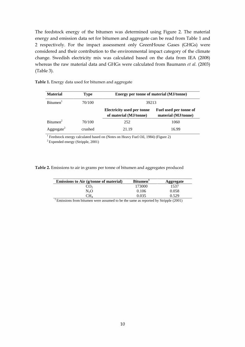
The feedstock energy of the bitumen was determined using Figure 2. The material

energy and emission data set for bitumen and aggregate can be read from Table 1 and

2 respectively. For the impact assessment only GreenHouse Gases (GHGs) were

considered and their contribution to the environmental impact category of the climate

change. Swedish electricity mix was calculated based on the data from IEA (2008)

whereas the raw material data and GHGs were calculated from Baumann et al. (2003)

(Table 3).

Table 1. Energy data used for bitumen and aggregate

Table 2. Emissions to air in grams per tonne of bitumen and aggregates produced

Material Type Energy per tonne of material (MJ/tonne)

Bitumen1 70/100 39213

Electricity used per tonne

of material (MJ/tonne)

Fuel used per tonne of

material (MJ/tonne)

Bitumen2 70/100 252 1060

Aggregate2 crushed 21.19 16.99

1 Feedstock energy calculated based on (Notes on Heavy Fuel Oil, 1984) (Figure 2) 2 Expended energy (Stripple, 2001)

Emissions to Air (g/tonne of material) Bitumen1 Aggregate

CO2 173000 1537

N2O 0.106 0.058

CH4 0.035 0.529 1 Emissions from bitumen were assumed to be the same as reported by Stripple (2001)

11

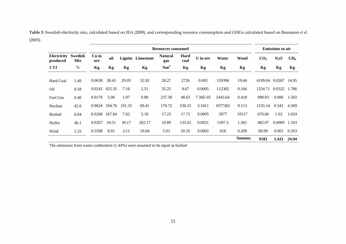
Table 3. Swedish electricity mix, calculated based on IEA (2008), and corresponding resource consumption and GHGs calculated based on Baumann et al.

(2003).

Resources consumed

Emissions to air

Electricity

produced

Swedish

Mix

Cu in

ore oil Lignite Limestone

Natural

gas

Hard

coal U in ore Water Wood

CO2 N2O CH4

1 TJ % Kg Kg Kg Kg Nm3 Kg Kg Kg Kg

Kg Kg Kg

Hard Coal 1.49 0.0638 38.43 29.05 32.92 28.27 2726 0.002 159396 19.66

4109.04 0.0267 14.95

Oil 0.58

0.0243 425.35 7.16 2.51 35.25 8.67 0.0005 112302 0.166

1334.71 0.0322 1.786

Fuel Gas 0.40 0.0176 5.06 1.07 0.80 237.58 48.63 7.36E-05 2443.64 0.418 988.03 0.006 1.502

Nuclear 42.6 0.9624 104.76 101.35 69.41 176.72 536.55 3.3411 1077365 9.113

1535.14 0.341 4.369

Biofuel 6.04 0.0268 167.84 7.62 5.18 17.23 17.71 0.0005 3977 10517

670.66 1.02 1.024

Hydro 46.1 0.0267 34.51 30.17 302.17 10.89 135.62 0.0021 5397.3 1.361

482.07 0.0069 1.103

Wind 1.33 0.5508 8.91 3.11 10.04 5.03 20.35 0.0002 618 0.209

60.90 0.001 0.203

Summa: 9181 1.431 24.94

The emissions from waste combustion (1.44%) were assumed to be equal as biofuel

12

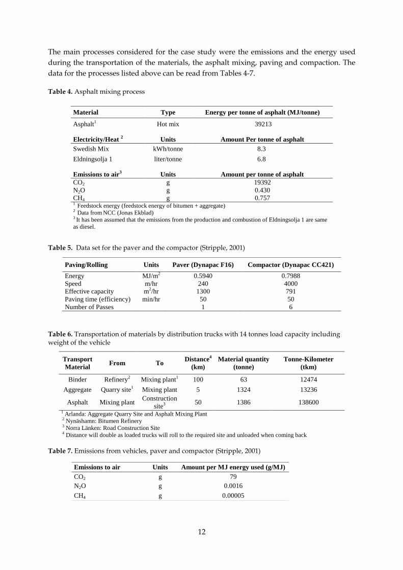
The main processes considered for the case study were the emissions and the energy used

during the transportation of the materials, the asphalt mixing, paving and compaction. The

data for the processes listed above can be read from Tables 4-7.

Table 4. Asphalt mixing process

Table 5. Data set for the paver and the compactor (Stripple, 2001)

Table 6. Transportation of materials by distribution trucks with 14 tonnes load capacity including weight of the vehicle

Table 7. Emissions from vehicles, paver and compactor (Stripple, 2001)

Material Type Energy per tonne of asphalt (MJ/tonne)

Asphalt1 Hot mix 39213

Electricity/Heat 2 Units Amount Per tonne of asphalt

Swedish Mix kWh/tonne 8.3

Eldningsolja 1 liter/tonne 6.8

Emissions to air3 Units Amount per tonne of asphalt

CO2 g 19392

N2O g 0.430

CH4 g 0.757 1 Feedstock energy (feedstock energy of bitumen + aggregate) 2 Data from NCC (Jonas Ekblad) 3 It has been assumed that the emissions from the production and combustion of Eldningsolja 1 are same

as diesel.

Paving/Rolling Units Paver (Dynapac F16) Compactor (Dynapac CC421)

Energy MJ/m2 0.5940 0.7988

Speed m/hr 240 4000

Effective capacity m2/hr 1300 791

Paving time (efficiency) min/hr 50 50

Number of Passes

1 6

Transport

Material From To

Distance4

(km)

Material quantity

(tonne)

Tonne-Kilometer

(tkm)

Binder Refinery2 Mixing plant

1 100 63 12474

Aggregate Quarry site1 Mixing plant 5 1324 13236

Asphalt Mixing plant Construction

site3

50 1386 138600

1 Arlanda: Aggregate Quarry Site and Asphalt Mixing Plant 2 Nynäshamn: Bitumen Refinery 3 Norra Länken: Road Construction Site 4 Distance will double as loaded trucks will roll to the required site and unloaded when coming back

Emissions to air Units Amount per MJ energy used (g/MJ)

CO2 g 79

N2O g 0.0016

CH4 g 0.00005

13

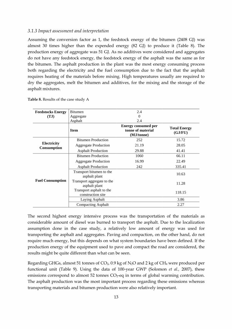
3.1.3 Impact assessment and interpretation

Assuming the conversion factor as 1, the feedstock energy of the bitumen (2408 GJ) was

almost 30 times higher than the expended energy (82 GJ) to produce it (Table 8). The

production energy of aggregate was 51 GJ. As no additives were considered and aggregates

do not have any feedstock energy, the feedstock energy of the asphalt was the same as for

the bitumen. The asphalt production in the plant was the most energy consuming process

both regarding the electricity and the fuel consumption due to the fact that the asphalt

requires heating of the materials before mixing. High temperatures usually are required to

dry the aggregates, melt the bitumen and additives, for the mixing and the storage of the

asphalt mixtures.

Table 8. Results of the case study A

Feedstocks Energy

(TJ)

Bitumen 2.4

Aggregate 0

Asphalt 2.4

Item

Energy consumed per

tonne of material

(MJ/tonne)

Total Energy

(GJ/FU)

Electricity

Consumption

Bitumen Production 252 15.72

Aggregate Production 21.19 28.05

Asphalt Production 29.88 41.41

Fuel Consumption

Bitumen Production 1060 66.11

Aggregate Production 16.99 22.49

Asphalt Production 242 335.41

Transport bitumen to the

asphalt plant 10.63

Transport aggregate to the

asphalt plant 11.28

Transport asphalt to the

construction site 118.15

Laying Asphalt

3.86

Compacting Asphalt

2.27

The second highest energy intensive process was the transportation of the materials as

considerable amount of diesel was burned to transport the asphalt. Due to the localization

assumption done in the case study, a relatively low amount of energy was used for

transporting the asphalt and aggregates. Paving and compaction, on the other hand, do not

require much energy, but this depends on what system boundaries have been defined. If the

production energy of the equipment used to pave and compact the road are considered, the

results might be quite different than what can be seen.

Regarding GHGs, almost 51 tonnes of CO2, 0.9 kg of N2O and 2 kg of CH4 were produced per

functional unit (Table 9). Using the data of 100-year GWP (Solomon et al., 2007), these

emissions correspond to almost 52 tonnes CO2-eq in terms of global warming contribution.

The asphalt production was the most important process regarding these emissions whereas

transporting materials and bitumen production were also relatively important.

14

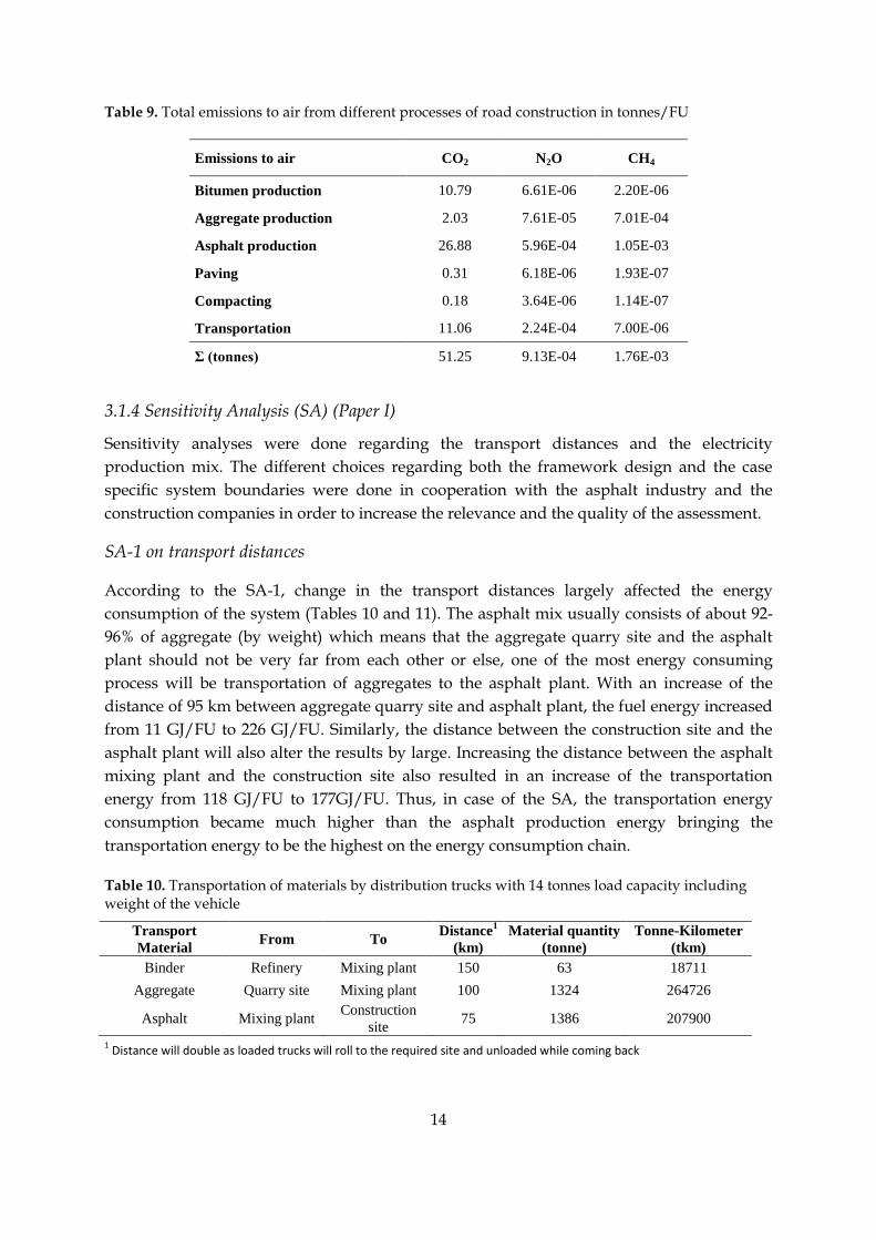
Table 9. Total emissions to air from different processes of road construction in tonnes/FU

3.1.4 Sensitivity Analysis (SA) (Paper I)

Sensitivity analyses were done regarding the transport distances and the electricity

production mix. The different choices regarding both the framework design and the case

specific system boundaries were done in cooperation with the asphalt industry and the

construction companies in order to increase the relevance and the quality of the assessment.

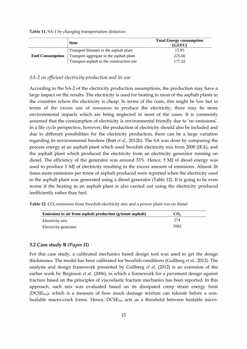
SA-1 on transport distances

According to the SA-1, change in the transport distances largely affected the energy

consumption of the system (Tables 10 and 11). The asphalt mix usually consists of about 92-

96% of aggregate (by weight) which means that the aggregate quarry site and the asphalt

plant should not be very far from each other or else, one of the most energy consuming

process will be transportation of aggregates to the asphalt plant. With an increase of the

distance of 95 km between aggregate quarry site and asphalt plant, the fuel energy increased

from 11 GJ/FU to 226 GJ/FU. Similarly, the distance between the construction site and the

asphalt plant will also alter the results by large. Increasing the distance between the asphalt

mixing plant and the construction site also resulted in an increase of the transportation

energy from 118 GJ/FU to 177GJ/FU. Thus, in case of the SA, the transportation energy

consumption became much higher than the asphalt production energy bringing the

transportation energy to be the highest on the energy consumption chain.

Table 10. Transportation of materials by distribution trucks with 14 tonnes load capacity including weight of the vehicle

1 Distance will double as loaded trucks will roll to the required site and unloaded while coming back

Emissions to air CO2 N2O CH4

Bitumen production 10.79 6.61E-06 2.20E-06

Aggregate production 2.03 7.61E-05 7.01E-04

Asphalt production 26.88 5.96E-04 1.05E-03

Paving 0.31 6.18E-06 1.93E-07

Compacting 0.18 3.64E-06 1.14E-07

Transportation 11.06 2.24E-04 7.00E-06

Σ (tonnes) 51.25 9.13E-04 1.76E-03

Transport

Material From To

Distance1

(km)

Material quantity

(tonne)

Tonne-Kilometer

(tkm)

Binder Refinery Mixing plant 150 63 18711

Aggregate Quarry site Mixing plant 100 1324 264726

Asphalt Mixing plant Construction

site 75 1386 207900

15

Table 11. SA-1 by changing transportation distances

SA-2 on efficient electricity production and its use

According to the SA-2 of the electricity production assumptions, the production may have a

large impact on the results. The electricity is used for heating in most of the asphalt plants in

the countries where the electricity is cheap. In terms of the costs, this might be low but in

terms of the excess use of resources to produce the electricity; there may be more

environmental impacts which are being neglected in most of the cases. It is commonly

assumed that the consumption of electricity is environmental friendly due to ‘no emissions’.

In a life cycle perspective, however, the production of electricity should also be included and

due to different possibilities for the electricity production, there can be a large variation

regarding its environmental burdens (Butt et al., 2012b). The SA was done by comparing the

process energy at an asphalt plant which used Swedish electricity mix from 2008 (IEA), and

the asphalt plant which produced the electricity from an electricity generator running on

diesel. The efficiency of the generator was around 33%. Hence, 3 MJ of diesel energy was

used to produce 1 MJ of electricity resulting in the excess amount of emissions. Almost 26

times more emissions per tonne of asphalt produced were reported when the electricity used

in the asphalt plant was generated using a diesel generator (Table 12). It is going to be even

worse if the heating in an asphalt plant is also carried out using the electricity produced

inefficiently rather than fuel.

Table 12. CO2 emissions from Swedish electricity mix and a power plant run on diesel

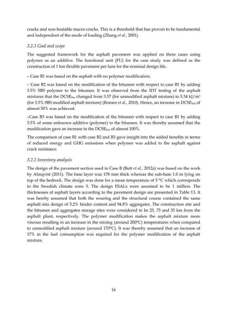
3.2 Case study B (Paper II)

For this case study, a calibrated mechanics based design tool was used to get the design

thicknesses. The model has been calibrated for Swedish conditions (Gullberg et al., 2012). The

analysis and design framework presented by Gullberg et al. (2012) is an extension of the

earlier work by Birgisson et al. (2006), in which a framework for a pavement design against

fracture based on the principles of viscoelastic fracture mechanics has been reported. In this

approach, each mix was evaluated based on its dissipated creep strain energy limit

(DCSElim), which is a measure of how much damage mixture can tolerate before a non-

healable macro-crack forms. Hence, DCSElim acts as a threshold between healable micro-

Item

Total Energy consumption

(GJ/FU)

Fuel Consumption

Transport bitumen to the asphalt plant 15.95

Transport aggregate to the asphalt plant 225.66

Transport asphalt to the construction site 177.22

Emissions to air from asphalt production (g/tonne asphalt) CO2

Electricity mix 274

Electricity generator 7082

16

cracks and non-healable macro-cracks. This is a threshold that has proven to be fundamental

and independent of the mode of loading (Zhang et al., 2001).

3.2.1 Goal and scope

The suggested framework for the asphalt pavement was applied on three cases using

polymer as an additive. The functional unit (FU) for the case study was defined as the

construction of 1 km flexible pavement per lane for the nominal design life.

– Case B1 was based on the asphalt with no polymer modification;

– Case B2 was based on the modification of the bitumen with respect to case B1 by adding

3.5% SBS polymer to the bitumen. It was observed from the IDT testing of the asphalt

mixtures that the DCSElim changed from 3.57 (for unmodified asphalt mixture) to 5.34 kJ/m3

(for 3.5% SBS modified asphalt mixture) (Romeo et al., 2010). Hence, an increase in DCSElim of

almost 50% was achieved.

–Case B3 was based on the modification of the bitumen with respect to case B1 by adding

3.5% of some unknown additive (polymer) to the bitumen. It was thereby assumed that the

modification gave an increase in the DCSElim of almost 100%.

The comparison of case B1 with case B2 and B3 gave insight into the added benefits in terms

of reduced energy and GHG emissions when polymer was added to the asphalt against

crack resistance.

3.2.2 Inventory analysis

The design of the pavement section used in Case B (Butt et al., 2012a) was based on the work

by Almqvist (2011). The base layer was 178 mm thick whereas the sub-base 1.0 m lying on

top of the bedrock. The design was done for a mean temperature of 5 °C which corresponds

to the Swedish climate zone 3. The design ESALs were assumed to be 1 million. The

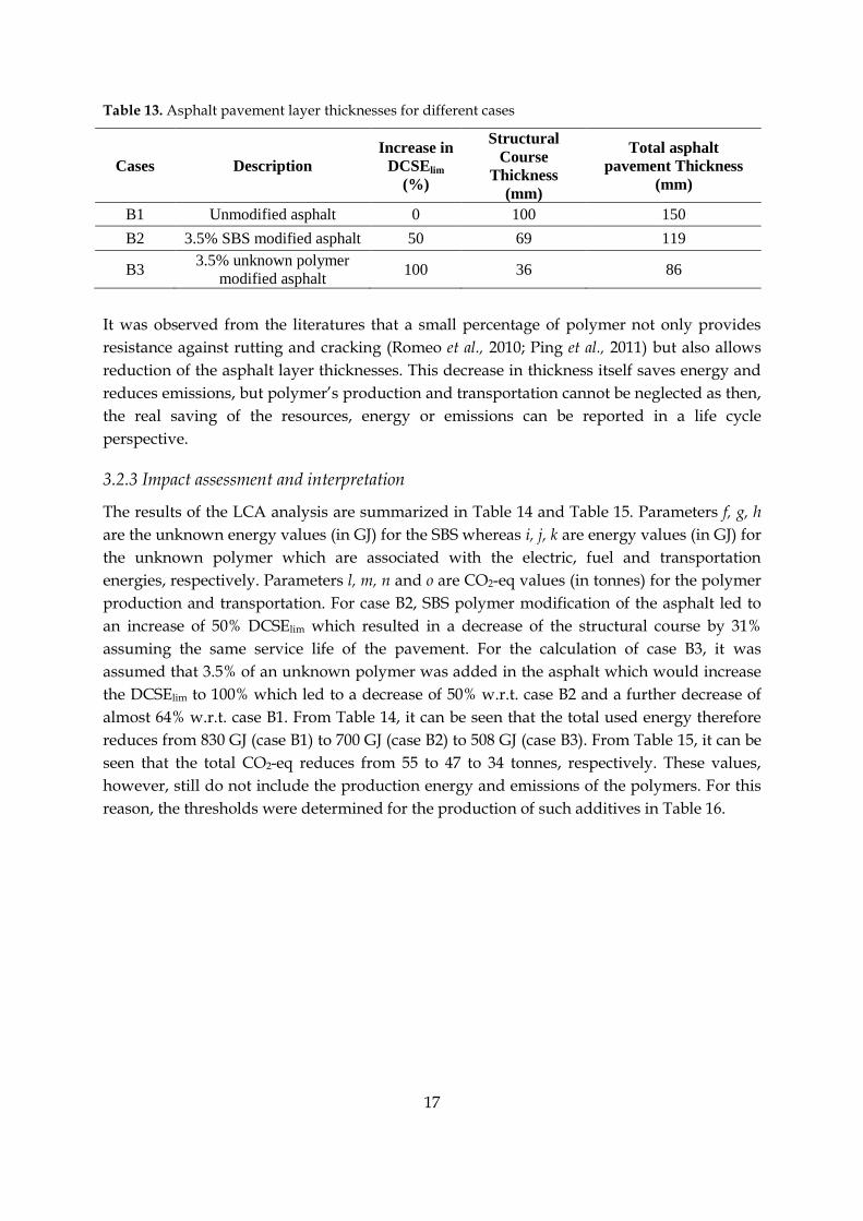
thicknesses of asphalt layers according to the pavement design are presented in Table 13. It

was hereby assumed that both the wearing and the structural course contained the same

asphalt mix design of 5.2% binder content and 94.8% aggregates. The construction site and

the bitumen and aggregates storage sites were considered to be 25, 75 and 35 km from the

asphalt plant, respectively. The polymer modification makes the asphalt mixture more

viscous resulting in an increase in the mixing (around 200°C) temperatures when compared

to unmodified asphalt mixture (around 170°C). It was thereby assumed that an increase of

17% in the fuel consumption was required for the polymer modification of the asphalt

mixture.

17

Table 13. Asphalt pavement layer thicknesses for different cases

Cases Description

Increase in

DCSElim

(%)

Structural

Course

Thickness

(mm)

Total asphalt

pavement Thickness

(mm)

B1 Unmodified asphalt 0 100 150

B2 3.5% SBS modified asphalt 50 69 119

B3 3.5% unknown polymer

modified asphalt 100 36 86

It was observed from the literatures that a small percentage of polymer not only provides

resistance against rutting and cracking (Romeo et al., 2010; Ping et al., 2011) but also allows

reduction of the asphalt layer thicknesses. This decrease in thickness itself saves energy and

reduces emissions, but polymer’s production and transportation cannot be neglected as then,

the real saving of the resources, energy or emissions can be reported in a life cycle

perspective.

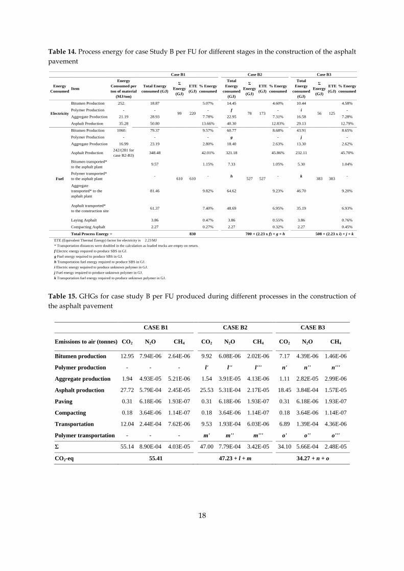
3.2.3 Impact assessment and interpretation

The results of the LCA analysis are summarized in Table 14 and Table 15. Parameters f, g, h

are the unknown energy values (in GJ) for the SBS whereas i, j, k are energy values (in GJ) for

the unknown polymer which are associated with the electric, fuel and transportation

energies, respectively. Parameters l, m, n and o are CO2-eq values (in tonnes) for the polymer

production and transportation. For case B2, SBS polymer modification of the asphalt led to

an increase of 50% DCSElim which resulted in a decrease of the structural course by 31%

assuming the same service life of the pavement. For the calculation of case B3, it was

assumed that 3.5% of an unknown polymer was added in the asphalt which would increase

the DCSElim to 100% which led to a decrease of 50% w.r.t. case B2 and a further decrease of

almost 64% w.r.t. case B1. From Table 14, it can be seen that the total used energy therefore

reduces from 830 GJ (case B1) to 700 GJ (case B2) to 508 GJ (case B3). From Table 15, it can be

seen that the total CO2-eq reduces from 55 to 47 to 34 tonnes, respectively. These values,

however, still do not include the production energy and emissions of the polymers. For this

reason, the thresholds were determined for the production of such additives in Table 16.

18

CASE B1 CASE B2 CASE B3

Emissions to air (tonnes) CO2 N2O CH4

CO2 N2O CH4

CO2 N2O CH4

Bitumen production 12.95 7.94E-06 2.64E-06

9.92 6.08E-06 2.02E-06

7.17 4.39E-06 1.46E-06

Polymer production - - -

l' l'' l'''

n' n'' n'''

Aggregate production 1.94 4.93E-05 5.21E-06

1.54 3.91E-05 4.13E-06

1.11 2.82E-05 2.99E-06

Asphalt production 27.72 5.79E-04 2.45E-05

25.53 5.31E-04 2.17E-05

18.45 3.84E-04 1.57E-05

Paving 0.31 6.18E-06 1.93E-07

0.31 6.18E-06 1.93E-07

0.31 6.18E-06 1.93E-07

Compacting 0.18 3.64E-06 1.14E-07

0.18 3.64E-06 1.14E-07

0.18 3.64E-06 1.14E-07

Transportation 12.04 2.44E-04 7.62E-06

9.53 1.93E-04 6.03E-06

6.89 1.39E-04 4.36E-06

Polymer transportation - - -

m' m'' m'''

o' o'' o'''

Σ 55.14 8.90E-04 4.03E-05

47.00 7.79E-04 3.42E-05

34.10 5.66E-04 2.48E-05

CO2-eq 55.41 47.23 + l + m 34.27 + n + o

Table 14. Process energy for case Study B per FU for different stages in the construction of the asphalt

pavement

Table 15. GHGs for case study B per FU produced during different processes in the construction of

the asphalt pavement

Case B1

Case B2

Case B3

Energy

Consumed Item

Energy

Consumed per

ton of material

(MJ/ton)

Total Energy

consumed (GJ)

Σ

Energy

(GJ)

ETE

(GJ)

% Energy

consumed

Total

Energy

consumed

(GJ)

Σ

Energy

(GJ)

ETE

(GJ)

% Energy

consumed

Total

Energy

consumed

(GJ)

Σ

Energy

(GJ)

ETE

(GJ)

% Energy

consumed

Electricity

Bitumen Production 252.00 18.87

99 220

5.07%

14.45

78 173

4.60%

10.44

56 125

4.58%

Polymer Production - - -

f -

i -

Aggregate Production 21.19 28.93 7.78%

22.95 7.31%

16.58 7.28%

Asphalt Production 35.28 50.80 13.66%

40.30 12.83%

29.13 12.79%

Fuel

Bitumen Production 1060.00 79.37

610 610

9.57%

60.77

527 527

8.68%

43.91

383 383

8.65%

Polymer Production - - -

g -

j -

Aggregate Production 16.99 23.19 2.80%

18.40 2.63%

13.30 2.62%

Asphalt Production 242/(281 for

case B2-B3) 348.48 42.01%

321.18 45.86%

232.11 45.70%

Bitumen transported*

to the asphalt plant 9.57 1.15%

7.33 1.05%

5.30 1.04%

Polymer transported*

to the asphalt plant - -

h -

k -

Aggregate

transported* to the

asphalt plant

81.46 9.82%

64.62 9.23%

46.70 9.20%

Asphalt transported*

to the construction site 61.37 7.40%

48.69 6.95%

35.19 6.93%

Laying Asphalt

3.86 0.47%

3.86 0.55%

3.86 0.76%

Compacting Asphalt

2.27 0.27%

2.27 0.32%

2.27 0.45%

Total Process Energy = 830

700 + (2.23 x f) + g + h

508 + (2.23 x i) + j + k

ETE (Equivalent Thermal Energy) factor for electricity is 2.23 MJ

* Transportation distances were doubled in the calculation as loaded trucks are empty on return.

f Electric energy required to produce SBS in GJ.

g Fuel energy required to produce SBS in GJ.

h Transportation fuel energy required to produce SBS in GJ.

i Electric energy required to produce unknown polymer in GJ.

j Fuel energy required to produce unknown polymer in GJ.

k Transportation fuel energy required to produce unknown polymer in GJ.

19

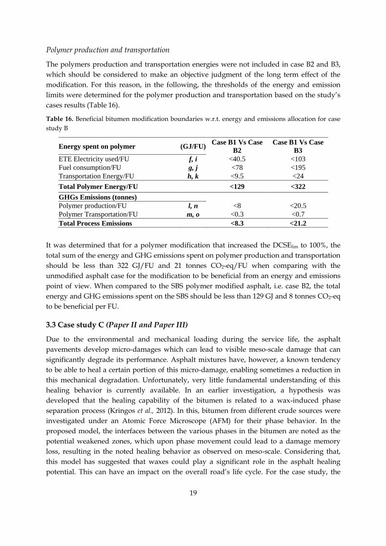
Polymer production and transportation

The polymers production and transportation energies were not included in case B2 and B3,

which should be considered to make an objective judgment of the long term effect of the

modification. For this reason, in the following, the thresholds of the energy and emission

limits were determined for the polymer production and transportation based on the study’s

cases results (Table 16).

Table 16. Beneficial bitumen modification boundaries w.r.t. energy and emissions allocation for case

study B

Energy spent on polymer (GJ/FU) Case B1 Vs Case

B2

Case B1 Vs Case

B3

ETE Electricity used/FU f, i <40.5 <103

Fuel consumption/FU g, j <78 <195

Transportation Energy/FU h, k <9.5 <24

Total Polymer Energy/FU

<129 <322

GHGs Emissions (tonnes)

Polymer production/FU l, n <8 <20.5

Polymer Transportation/FU m, o <0.3 <0.7

Total Process Emissions <8.3 <21.2

It was determined that for a polymer modification that increased the DCSElim to 100%, the

total sum of the energy and GHG emissions spent on polymer production and transportation

should be less than 322 GJ/FU and 21 tonnes CO2-eq/FU when comparing with the

unmodified asphalt case for the modification to be beneficial from an energy and emissions

point of view. When compared to the SBS polymer modified asphalt, i.e. case B2, the total

energy and GHG emissions spent on the SBS should be less than 129 GJ and 8 tonnes CO2-eq

to be beneficial per FU.

3.3 Case study C (Paper II and Paper III)

Due to the environmental and mechanical loading during the service life, the asphalt

pavements develop micro-damages which can lead to visible meso-scale damage that can

significantly degrade its performance. Asphalt mixtures have, however, a known tendency

to be able to heal a certain portion of this micro-damage, enabling sometimes a reduction in

this mechanical degradation. Unfortunately, very little fundamental understanding of this

healing behavior is currently available. In an earlier investigation, a hypothesis was

developed that the healing capability of the bitumen is related to a wax-induced phase

separation process (Kringos et al., 2012). In this, bitumen from different crude sources were

investigated under an Atomic Force Microscope (AFM) for their phase behavior. In the

proposed model, the interfaces between the various phases in the bitumen are noted as the

potential weakened zones, which upon phase movement could lead to a damage memory

loss, resulting in the noted healing behavior as observed on meso-scale. Considering that,

this model has suggested that waxes could play a significant role in the asphalt healing

potential. This can have an impact on the overall road’s life cycle. For the case study, the

20

hypothesis was made that the benefit of having self-healing bitumen in the pavement would

lead to a lighter pavement design for the same service life time of a pavement.

3.3.1 Goal and scope

The suggested framework for the asphalt pavement was applied on the three cases. The FU

defined for this case study was the construction of a 1 km long and 3.5 m wide asphalt

pavement for the stated design life.

Case C1 was based on bitumen that was assumed to have no healing capacity;

Case C2 was based on the assumption that the bitumen had in fact known capability

for an intrinsic healing mechanism, without the need for any additional modification.

This healing capacity was giving a ‘free’ 10% increase of the pavement lifetime with

comparison to the ‘non-healing’ case C1;

Case C3 was based on modification of the bitumen with respect to case C1 by adding

4% Montan wax to the bitumen. This was giving the pavement an added 10%

increase of the lifetime; similar to case C2, but in this case the bitumen did not have a

natural healing tendency and had to be modified.

The comparison between cases C1 and C2 would give insight into the added benefits in

terms of reduced energy and GHG emissions when the used bitumen has an intrinsic healing

capacity. Here the assumption was made that exactly the same bitumen was used in both

cases. The comparison between cases C1 and C3 would enable balancing the pro’s and con’s

of extra energy and emissions due to modifying the bitumen with the added lifetime

benefits.

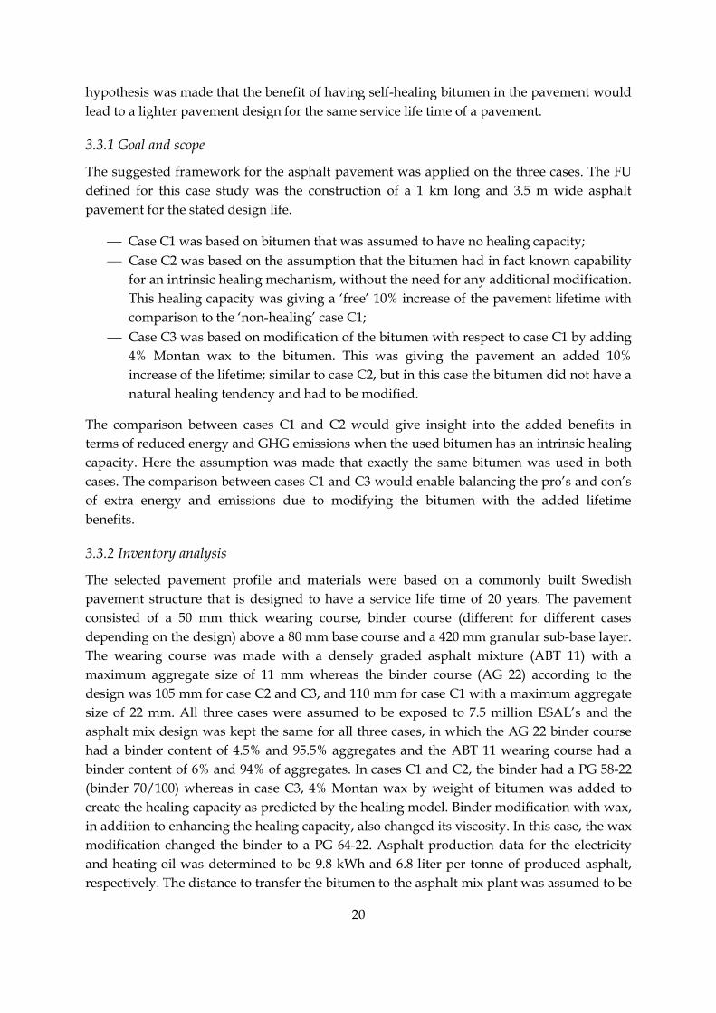
3.3.2 Inventory analysis

The selected pavement profile and materials were based on a commonly built Swedish

pavement structure that is designed to have a service life time of 20 years. The pavement

consisted of a 50 mm thick wearing course, binder course (different for different cases

depending on the design) above a 80 mm base course and a 420 mm granular sub-base layer.

The wearing course was made with a densely graded asphalt mixture (ABT 11) with a

maximum aggregate size of 11 mm whereas the binder course (AG 22) according to the

design was 105 mm for case C2 and C3, and 110 mm for case C1 with a maximum aggregate

size of 22 mm. All three cases were assumed to be exposed to 7.5 million ESAL’s and the

asphalt mix design was kept the same for all three cases, in which the AG 22 binder course

had a binder content of 4.5% and 95.5% aggregates and the ABT 11 wearing course had a

binder content of 6% and 94% of aggregates. In cases C1 and C2, the binder had a PG 58-22

(binder 70/100) whereas in case C3, 4% Montan wax by weight of bitumen was added to

create the healing capacity as predicted by the healing model. Binder modification with wax,

in addition to enhancing the healing capacity, also changed its viscosity. In this case, the wax

modification changed the binder to a PG 64-22. Asphalt production data for the electricity

and heating oil was determined to be 9.8 kWh and 6.8 liter per tonne of produced asphalt,

respectively. The distance to transfer the bitumen to the asphalt mix plant was assumed to be

21

100 km, whereas the transfer of the asphalt mixtures to the construction site was taken as 50

km. The aggregate quarry site and the asphalt mix plant were hereby assumed to be at the

same location, 5 km from each other.

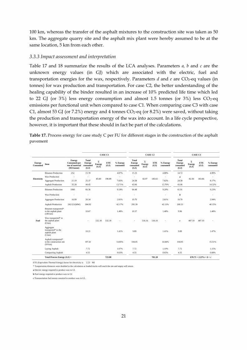
3.3.3 Impact assessment and interpretation

Table 17 and 18 summarize the results of the LCA analyses. Parameters a, b and c are the

unknown energy values (in GJ) which are associated with the electric, fuel and

transportation energies for the wax, respectively. Parameters d and e are CO2-eq values (in

tonnes) for wax production and transportation. For case C2, the better understanding of the

healing capability of the binder resulted in an increase of 10% predicted life time which led

to 22 GJ (or 3%) less energy consumption and almost 1.5 tonnes (or 3%) less CO2-eq

emissions per functional unit when compared to case C1. When comparing case C3 with case

C1, almost 53 GJ (or 7.2%) energy and 4 tonnes CO2-eq (or 8.2%) were saved, without taking

the production and transportation energy of the wax into account. In a life cycle perspective,

however, it is important that these should in fact be part of the calculations.

Table 17. Process energy for case study C per FU for different stages in the construction of the asphalt

pavement

CASE C1

CASE C2

CASE C3

Energy

Consumed Item

Energy

Consumed per

ton of material

(MJ/tonne)

Total

Energy

consumed

(GJ)

Σ

Energy

(GJ)

ETE

(GJ)

% Energy

consumed

Total

Energy

consumed

(GJ)

Σ

Energy

(GJ)

ETE

(GJ)

% Energy

consumed

Total

Energy

consumed

(GJ)

Σ

Energy

(GJ)

ETE

(GJ)

% Energy

consumed

Electricity

Bitumen Production 252.00 15.78

85.60 190.89

4.87%

15.33

82.97 185.02

4.88%

14.72

82.36 183.66

4.89%

Wax Production - - -

- -

a -

Aggregate Production 21.19 25.37 7.83%

24.58 7.82%

24.58 8.17%

Asphalt Production 35.28 44.45 13.71%

43.06 13.70%

43.06 14.32%

Fuel

Bitumen Production 1060.00 66.36

532.18 532.18

9.18%

64.48

516.16 516.16

9.20%

61.91

487.10 487.10

9.23%

Wax Production - - -

- -

b -

Aggregate Production 16.99 20.34 2.81%

19.70 2.81%

19.70 2.94%

Asphalt Production 242/221(MW) 304.92 42.17%

295.39 42.13%

269.33 40.15%

Bitumen transported*

to the asphalt plant

(100 km)

10.67 1.48%

10.37 1.48%

9.96 1.48%

Wax transported* to

the asphalt plant

(0 km)

- -

- -

c -

Aggregate

transported* to the

asphalt plant (5 km)

10.21 1.41%

9.89 1.41%

9.89 1.47%

Asphalt transported* to the construction site

(50 km)

107.41 14.85%

104.05 14.84%

104.05 15.51%

Laying Asphalt

7.72 1.07%

7.72 1.10%

7.72 1.15%

Compacting Asphalt

4.55 0.63%

4.55 0.65%

4.55 0.68%

Total Process Energy (GJ) = 723.08

701.18

670.75 + 2.23*a + b + c

ETE (Equivalent Thermal Energy) factor for electricity is 2.23 MJ

* Tranportation distances were doubled in the calculation as loaded trucks will reach the site and empty will return.

a Electric energy required to produce wax in GJ.

b Fuel energy required to produce wax in GJ.

c Transportation fuel energy required to produce wax in GJ.

22

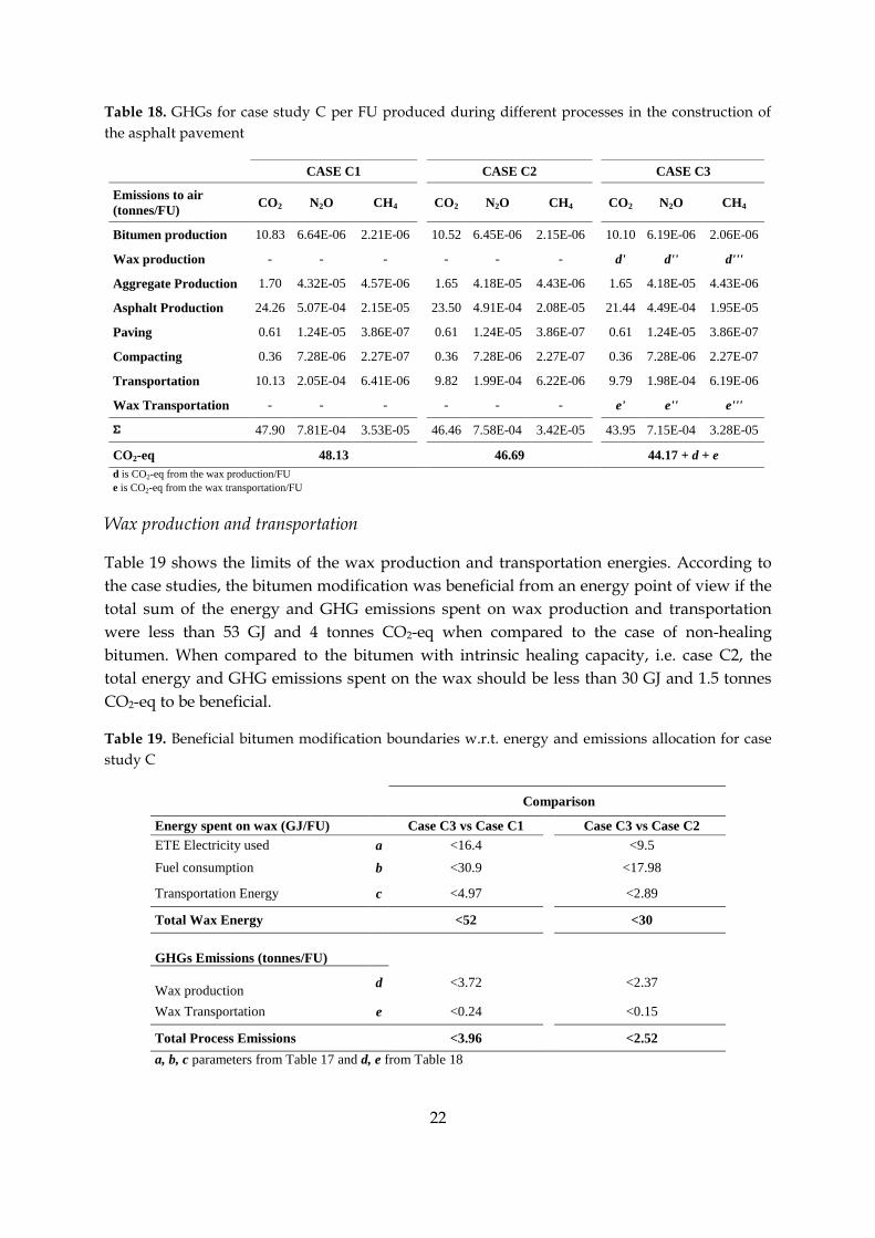
Table 18. GHGs for case study C per FU produced during different processes in the construction of

the asphalt pavement

Wax production and transportation

Table 19 shows the limits of the wax production and transportation energies. According to

the case studies, the bitumen modification was beneficial from an energy point of view if the

total sum of the energy and GHG emissions spent on wax production and transportation

were less than 53 GJ and 4 tonnes CO2-eq when compared to the case of non-healing

bitumen. When compared to the bitumen with intrinsic healing capacity, i.e. case C2, the

total energy and GHG emissions spent on the wax should be less than 30 GJ and 1.5 tonnes

CO2-eq to be beneficial.

Table 19. Beneficial bitumen modification boundaries w.r.t. energy and emissions allocation for case

study C

CASE C1

CASE C2

CASE C3

Emissions to air

(tonnes/FU) CO2 N2O CH4

CO2 N2O CH4 CO2 N2O CH4

Bitumen production 10.83 6.64E-06 2.21E-06

10.52 6.45E-06 2.15E-06

10.10 6.19E-06 2.06E-06

Wax production - - -

- - -

d' d'' d'''

Aggregate Production 1.70 4.32E-05 4.57E-06

1.65 4.18E-05 4.43E-06

1.65 4.18E-05 4.43E-06

Asphalt Production 24.26 5.07E-04 2.15E-05

23.50 4.91E-04 2.08E-05

21.44 4.49E-04 1.95E-05

Paving 0.61 1.24E-05 3.86E-07

0.61 1.24E-05 3.86E-07

0.61 1.24E-05 3.86E-07

Compacting 0.36 7.28E-06 2.27E-07

0.36 7.28E-06 2.27E-07

0.36 7.28E-06 2.27E-07

Transportation 10.13 2.05E-04 6.41E-06

9.82 1.99E-04 6.22E-06

9.79 1.98E-04 6.19E-06

Wax Transportation - - -

- - -

e' e'' e'''

Σ 47.90 7.81E-04 3.53E-05

46.46 7.58E-04 3.42E-05

43.95 7.15E-04 3.28E-05

CO2-eq 48.13

46.69

44.17 + d + e

d is CO2-eq from the wax production/FU

e is CO2-eq from the wax transportation/FU

Comparison

Energy spent on wax (GJ/FU) Case C3 vs Case C1 Case C3 vs Case C2

ETE Electricity used a <16.4 <9.5

Fuel consumption b <30.9 <17.98

Transportation Energy c <4.97 <2.89

Total Wax Energy

<52 <30

GHGs Emissions (tonnes/FU)

Wax production d <3.72 <2.37

Wax Transportation e <0.24 <0.15

Total Process Emissions <3.96 <2.52

a, b, c parameters from Table 17 and d, e from Table 18

23

4. Conclusions

In this work, an open LCA framework is suggested for quantifying energy and

environmental loads during construction, maintenance and end of life phases of a given

asphalt pavement. A method to calculate feedstock energy of bitumen is developed and a

method to quantify mass-energy flows of additives is described. If the production data of

additives is available, an energy-mass flow of any asphalt additive can be calculated based

on the method suggested. Such calculations for waxes and polymers should be valuable in

order to determine the life cycle benefits from using such additives. However, this would

require information on electricity and fuel usage. Regarding feedstock energy in the binder,

it is highly relevant for the LCC as the cost of the binder will be reflected in its alternative

value as fuel. For LCAs, however, it is suggested to be of a limited importance although it

may be used to quantify the resource energy.

From the case studies, it could be concluded that asphalt production is a highly energy

consuming process. Hence, the use of additives should be further studied in order to

determine their potential to decrease energy use through lowering the mixing temperatures.

Transportation of the materials plays a very important role in terms of energy consumption

and emissions. It is favourable to have quarry site, asphalt production plant and the

construction site not far from each other to avoid excess energy use and fuel combustion

emissions. It is also highly favourable to use electricity that has been produced in an efficient

way.

From the case studies, it can be concluded that better understanding of the binder provides

bases for better pavement design optimization, hence reducing the energy consumption and

emissions. A limit in terms of energy and emissions for the production of the wax and

polymers was also found which could help the additive producers to improve their

manufacturing processes making them efficient enough to be beneficial from a pavement life

cycle point of view. In other words: positive effects obtained due to the use of additives are

only beneficial when the energy and emissions are lower in comparison to the unmodified

asphalt when considering the life cycle of a road. Hence, the binder self-healing capability

and the use of additives like polymers and waxes should be further studied in order to

determine the benefits which could be achieved in terms of the resource consumption,

energy and emissions by lowering the energy utilization in the asphalt mix plant. This would

also help the road authorities in setting ‘green’ limits to get a real benefit from the additives

over the lifetime of a road.

It is not possible to make the infrastructure sector more environmentally conscious unless we

have a tool that takes all the associated aspects into consideration. Otherwise, new

technologies that, for example, may reduce CO2 emissions on one end and may reduce the

pavement sustainability on the other, thus resulting in an overall situation that is not

beneficial from an environmental perspective.

24

References

Almqvist, Y. (2011), Nedbrytning av vägar: Jämförelse mellan axlar med singel- respektive

tvillingmontage, Master thesis, TRITA-VBT 11:06, Royal Institute of Technology KTH,

Stockholm, Sweden.

Baumann, H. and Tillman, A.M. (2003), The Hitch Hiker's guide to LCA, An Orientataion in LCA

methodology and application, Göteborg: Studentlitteratur.

Birgisson, B., Wang, J. and Roque, R. (2006), Implementation of the Florida Cracking Model into the

Mechanistic-Empirical Pavement Design, Report no. UF #0003932, December, Gainesville:

University of Florida.

Birgisdóttir, H. (2005), Life cycle assessment model for road construction and use of residues from waste

incineration, PhD Thesis, Institute of Environment and Resources, Technical University of

Denmark DTU, Denmark.

Butt, A.A., Jelagin, D., Birgisson, B. and Kringos, N. (2012a), “Using Life Cycle Assessment to

Optimize Pavement Crack-Mitigation”, Scarpas et al. (Eds.), 7th RILEM International Conference

on Cracking in Pavements, Vol. 1, 20-22 June, Delft, Netherlands, p. 299-306.

Butt, A.A., Mirzadeh, I., Toller, S. and Birgisson, B. (2012b), “Bitumen Feedstock Energy and

Electricity Production in Pavement LCA”, ISAP 2012 international Symposium on Heavy Duty

Asphalt Pavements and Bridge Deck Pavements, 23-25 May, Nanjing, China.

Faber, J. (2002), Towards small scale use of asphalt as a fuel: an application of interest to developing

countries, Chemiewinkel Rapport C102, University of Groningen, The Netherlands.

Garg, A., Kazunari, K. and Pulles, T. (2006), 2006 IPCC Guidelines for the National Greenhouse Gas

Inventories, Intergovernmental Panel on Climate Change.

Gullberg, D., Birgisson, B. and Jelagin, D. (2012), “Evaluation of a novel calibrated-mechanistic

model to design against fracture under Swedish conditions”, International Journal of Road

Materials and Pavement Design, Vol. 13, issue 1, p. 49-66.

Herold, A. (2003), “Comparison of CO2 emission factors for fuels used in Greenhouse Gas

Inventories and consequences for monitoring and reporting under the EC emissions trading

scheme”, European Toxic Center on Air and Climatic Change, ETC/ACC Technical paper

2003/10.

Huang, Y., Bird, R. and Heidrich, O. (2009), “Development of a life cycle assessment tool for

construction and maintenance of asphalt pavements”, Journal of Cleaner Production, p. 283-296.

IEA, Electricity/Heat in Sweden in 2008. International Energy Agency:

http://www.iea.org/stats/electricitydata.asp?COUNTRY_CODE=SE [Accessed 29 August

2011]

25

Kringos, N., Pauli, T., Schmets, A. and Scarpas, A. (2012), “Demonstration of a New

Computational Model to Simulate Healing in Bitumen”, Journal of Association of Asphalt Paving

Technologists, under review.

Notes on Heavy Fuel Oil (1984), American Bureau of Shipping, ABS, publication 31 in January

1984.

NPC (2007), Working document of the National Petroleum Council (NPC) Global Oil and Gas

Study, (18th July 2007) [online], Available from: http://www.npc.org/study_topic_papers/8-

stg-biomass.pdf [Accessed 13 June 2012]

Ping, G.V. and Xiao, Y. (2011), In: Challenges and Recent Advances in Transportation

Engineering, ICTPA 24th Annual Conference & NACGEA International Symposium on Geo-Trans,

Paper No. S2-001, Los Angeles, CA, USA.

Romeo, E., Birgisson, B., Montepara, A. and Tebaldi, G. (2010), “The effect of polymer

modification on hot mix asphalt fracture at tensile loading conditions”, International Journal of

Pavement Engineering, Vol. 11, no. 5, p. 403-413.

Santero, N., Kendall, A., Harvey, J., Wang, T. and Lee, I. (2010a), Environmental Life-Cycle

Assessment for Asphalt Pavements: Issues and Recommended Future Directions, ISAP,

Nagoya, Japan.

Santero, N., Masanet, E. and Horvath, A. (2010b), LCA of Pavements: A critical review of existing

literature and research, Portland Cement Association, Skokie, Illinois, USA.

Solomon, S., Qin, D., Manning, M., Chen, Z., Marquis, M., Averyt, K.B., Tignor, M. and Miller,

H.L. (eds.) (2007), Intergovernmental Panel on Climate Change (IPCC), Fourth Assessment Report

(AR4), Working Group 1 (WG1), Chapter 2, Changes in Atmospheric Constituents and in

Radiative Forcing, Table 2.14, p. 212.

Stripple, H. (2001), Life Cycle Assessment of Road, A Pilot Study for Inventory Analysis, IVL Swedish

Environmental Research Institute, Second Revised Edition in March, Göteborg, Sweden.

Van Oers, L., De Koning, A., Guinée, J. and Huppes, G. (2002), Abiotic resource depletion in LCA;

Improving characterisation factors abiotic resource depletion as recommended in the new Dutch LCA

handbook, RWS-DWW report 2002-061, CML-Industrial Ecology, Leiden.

VTT, Measurements made by VTT communities and infrastructure. Finland.

Zapata, P. and Gambatese, J. (2005), “Energy Consumption of Asphalt and Reinforced Concrete

Pavement Materials and Construction”, Journal of Infrastructure Systems, Vol. 11 no.1, p. 9-20.

Zhang, Z., Roque, R., Birgisson, B. and Sangpetngam, B. (2001), “Identification of suitable crack

growth law for asphalt mixtures using the Superpave Indirect Tensile test (IDT)”, Journal of the

Association of Asphalt Paving Technologists, Vol. 70, p. 206-241.