Embed Size (px)
Citation preview

Graduate Theses, Dissertations, and Problem Reports
2011
Life cycle analysis of forest carbon in the central appalachian Life cycle analysis of forest carbon in the central appalachian
region region
Pradip Saud West Virginia University
Follow this and additional works at: https://researchrepository.wvu.edu/etd
Recommended Citation Recommended Citation Saud, Pradip, "Life cycle analysis of forest carbon in the central appalachian region" (2011). Graduate Theses, Dissertations, and Problem Reports. 4781. https://researchrepository.wvu.edu/etd/4781
This Thesis is protected by copyright and/or related rights. It has been brought to you by the The Research Repository @ WVU with permission from the rights-holder(s). You are free to use this Thesis in any way that is permitted by the copyright and related rights legislation that applies to your use. For other uses you must obtain permission from the rights-holder(s) directly, unless additional rights are indicated by a Creative Commons license in the record and/ or on the work itself. This Thesis has been accepted for inclusion in WVU Graduate Theses, Dissertations, and Problem Reports collection by an authorized administrator of The Research Repository @ WVU. For more information, please contact [email protected].

LIFE CYCLE ANALYSIS OF FOREST CARBON IN THE CENTRAL APPALACHIAN
REGION
Pradip Saud
Thesis Submitted to the Davis College of Agriculture, Natural Resources and Design at West Virginia University
in partial fulfillment of the requirements for the degree of
Master of Science
in Forestry
Jingxin Wang, Ph.D., Committee Chairperson John R. Brooks, Ph.D.
Gary Miller, Ph.D.
Division of Forestry and Natural Resources
Morgantown, WV
2011
Keywords: carbon emissions; carbon balance; carbon credit; fossil fuel; energy consumption; harvesting system; hardwood processing.
ABSTRACT
LIFE CYCLE ANALYSIS OF FOREST CARBON IN THE CENTRAL APPALACHIAN REGION
Pradip Saud
Forest management and wood product processing activities such as harvesting,
transportation, and lumber processing consume fossil fuels and emit carbon dioxide. This emitted
carbon dioxide creates credit carbon balance which is usually overlooked while estimating the
carbon benefits from woody biomass and wood products. Accountability of carbon stored in
woody biomass and wood products varies when such carbon emissions are considered. Factors
such as, harvesting intensity, growth rate, dead trees and forest fires all affected the estimation of
forest carbon balance while harvesting system determines the carbon emission from fossil fuel
consumptions. Energy sources used in sawmills for electricity are also crucial in credit carbon
balance analysis. Therefore, this study assessed (1) forest carbon balance of the mixed
Appalachian hardwood forests and carbon emissions due to the use of fossil fuels in harvesting
systems in West Virginia, and (2) carbon balance in hardwood lumber processing in the central
Appalachian region. Data were obtained from a regional sawmill survey, public database and
relevant publications.
Forest carbon balance and carbon emission were analyzed within a life cycle inventory
framework of cradle to gate using sensitivity analysis and stochastic simulation. The results
showed that the annual carbon balance of the forests per hectare was not significantly affected by
carbon loss from the volume of removal, fire and dead trees. It was also found that carbon
emission from combustion of fossil fuel using manual harvesting system was less than using
mechanized harvesting systems. Though a minimal amount of carbon was emitted from
harvesting systems, the forest carbon displacement rate during timber processing was affected
largely by hauling compared to felling, processing, skidding and loading. Carbon emission
quantity from fuel consumption and forest carbon displacement rate were also affected by
harvest intensity, hauling, payload size, forest type, and machine productivity.
Credit carbon balance generated from lumber processing was statistically analyzed within
the gate to gate life cycle inventory framework. Stochastic simulation of carbon emission and its
impact on carbon balance and carbon flux during lumber processing were carried out under
different operational scenarios. Credit carbon balance from electricity consumption varied
among sawmills of different production levels and operation hours per week and also attributed
effect of different head saws, lighting types and air compressors used at sawmills. Credit carbon
balance significantly reduced the carbon accountability of the lumber in useful life period at first
order of decay of carbon. Substantial amount of carbon flux attributed from energy consumption
and exports of lumber reduced the carbon storage accountability of the lumber product. Increase
of the carbon accountability of the lumber products and decrease of the carbon flux ratio could
be achieved through using an efficient equipments at sawmills and an appropriate mixture of
energy sources for electricity supply.

iii
DEDICATION
I wish to dedicate this thesis to Kuladevata Ghatal, father Pushkar Saud and mother Narmada
Devi Saud who always inspire me to set goals. I am extremely indebted to my brother Tek
Badhadur Saud, sister Himalaya Saud and sister in-law Pushpa Saud for their love and care
through my study. Finally, I would like thank my friends Benktesh Das Sharma, Sabina
Dhungana, Ishwar Dhami and Sudhiksha Joshi, who helped in several ways during my studies
and stay at WVU.

iv
ACKNOWLEDGEMENTS
I would like to thank Dr. Jingxin Wang, my major professor, for providing funding, time, and his
continuous involvement in my academic upbringing as well as in my professional endeavors to
this point during my studies. It is my fortunate to work under Dr. Wang, whose guidance brought
my learning up to the current level. I would also like to give a special thank to Dr. John R.
Brooks and Dr. Gary Miller, for their technical contributions and academic support during my
years at West Virginia University. Similarly I am thankful to Dr. Benktesh Das Sharma, who
serves and deserves my utmost appreciation and gratitude for his continuous motivation and
support. I would like to thank Dr. Ben Dawson for his continuous support and motivation to
complete my research. I would like to thank Ishwar Dhami, Sudiksha Joshi, Suresh Shrestha, my
friends from Nepal for their gratitude in several of my important life events. I would also like to
thank David Summerfield, Peter Michael Jacobson and Nathan Sites who have been the finest
colleagues and supportive friends. I would like to thank all professors and staffs within the
Wood Science and Technology Program and colleagues at WVU for being better group of people
to spend my college years with.

v
TABLE OF CONTENTS
ABSTRACT ................................................................................................................................... ii
DEDICATION ............................................................................................................................... iii
ACKNOWLEDGEMENTS ........................................................................................................... iv
TABLE OF CONTENTS ............................................................................................................... v
LIST OF FIGURES ..................................................................................................................... viii 1. Introduction ............................................................................................................................... 1
References ....................................................................................................................................... 5
2. A LIFE CYCLE ANALYSIS OF FOREST CARBON BALANCE AND CO 2
EMISSIONS OF TIMBER HARVESTING IN WEST VIRGINIA ............................... 9
Abstract ......................................................................................................................................... 10
2 .1 Introduction ............................................................................................................................ 11
2.2 Materials and Methods ............................................................................................................ 14
2.2.1 Data .............................................................................................................................. 14
2.2.2 Forest Carbon Estimation ............................................................................................ 17
2.2.3 Forest Harvesting and Fuel Consumption.................................................................... 18
2.2.4 Carbon Emissions from Fuel Consumptions ............................................................... 20
2.2.5 Sensitivity Analysis ..................................................................................................... 22
2.3 Results and Discussion ........................................................................................................... 23
2.3.1 Forest Carbon Balance ..................................................................................................... 23
2.3.2 Carbon Emissions from Timber Harvesting and Transportation ..................................... 27
2.3.3 Carbon Displacement from Forest to Sawmill................................................................. 29
2.3.4 Sensitivity Analysis and Uncertainty of Carbon Emission .............................................. 31
2.4 Conclusions ............................................................................................................................. 37
References ..................................................................................................................................... 38
3. CARBON BALANCE ANALYSIS OF HARDWOOD LUMBER PROCESSING IN
CENTRAL APPALACHIA .......................................................................................................... 44
Abstract ......................................................................................................................................... 45
3.1 Introduction ............................................................................................................................. 46
3.2 Methodology ........................................................................................................................... 49
3.2.1 Methodological Framework and System Boundary ........................................................ 49
3.2.2 Carbon Emission from Energy Sources ........................................................................... 50
3.2.3 Carbon in Lumber and Mill Residue ............................................................................... 52
3.2.4 Avoided Carbon Emission ............................................................................................... 55
3.2.5 Sawmill Processing Assessments .................................................................................... 56
3.3 Results and Discussion ........................................................................................................... 57
3.3.1 Carbon Emission from Electricity Consumption ............................................................. 57
3.3.2 Carbon Emission and Energy Capture ............................................................................. 59
3.3.3 Energy Efficient Equipment and Avoided Carbon Emission .......................................... 61

vi
3.3.4 Carbon Balance in Lumber Production ............................................................................ 65
3.3.5 Carbon Flux from lumber processing .............................................................................. 69
3.3.6 Sensitivity Analysis of Carbon Emission from Lumber Processing ................................ 69
3.3.7 Scenario Analysis of Carbon Flux from Lumber Processing .......................................... 72
3.3.8 Carbon Emission under Different Energy Sources .......................................................... 74
3.4. Conclusions ............................................................................................................................ 76
References ..................................................................................................................................... 77
4. SUMMARY .............................................................................................................................. 82

vii
LIST OF TABLES
Table 2. 1 Machine productivity and fuel consumption rate. ....................................................... 20
Table 2. 2 Annual C emissions (in thousand tons) in harvesting mixed hardwood species. ........ 28
Table 2. 3 C emissions from fossil fuel due to harvesting hardwood species by harvesting
function. ................................................................................................................................ 29
Table 3. 1 Carbon emission from all energy sources. ................................................................... 51
Table 3. 2 Descriptive statistics of lumber production and electricity consumption. ................... 58
Table 3. 3 Descriptive statistics of the efficient technique utilization in sawmill types. .............. 62

viii
LIST OF FIGURES
Figure 2.1 Life cycle inventory framework and system boundary. .............................................. 16
Figure 2.2 Predicted trends of carbon growth and carbon balance for 100 years. ........................ 26
Figure 2.3 Stochastic simulation of carbon balance from net stock and growth rate (tC/ha). ...... 26
Figure 2.4 Carbon displacements of four different forest type from the timber harvesting systems
and the generated residue extraction system. (a) and (b) timber harvesting under
mechanized and manual harvesting systems. (c) and (d) residue extracting under cable and
grappler skidding systems. .................................................................................................... 30
Figure 2.5 Carbon emission variations during skidding and hauling of mixed hardwood species.
(a) by skidder types and skidding distance (meters) and (b) by truck type and hauling
distance (km). ........................................................................................................................ 32
Figure 2.6 Carbon displacement rate variations from hauling process by different payload size
(m3) at different distances. (a) Mixed hardwood forest species (b) Oak-hickory forest group
(c) Ash-cottonwood forest group and (d) Maple-beech-birch forest group. ........................ 33
Figure 2.7 Trace plot and probability density plot of carbon emission (tC/TCM) using
mechanized (a) and (b) and manual (c) and (d) harvesting systems in the base case scenario.
............................................................................................................................................... 34
Figure 2.8 Probability density of carbon emission (tC /TCM) using mechanized (a, c, e) and
manual harvesting systems (b, d, f) at three different hauling distance i.e. 160 km (a, b), 240
km (c, d) and 320 km (e, f). .................................................................................................. 36 Figure 3. 1 Methodological framework and system boundary using LCI method. ...................... 54
Figure 3. 2 Diagnostic plots of the predictors to estimate the yearly C emission from sawmill. . 59
Figure 3. 3 Carbon emissions with and without energy capture process from sawmill. .............. 61
Figure 3. 4 Diagnostic plot of variability of carbon emission (tC) per TCM of lumber processing
by sawmill size at 95% prediction interval on the random effect of efficient techniques: (a)
head saw types, (b) lighting bulb types, and (c) air compressor types. ................................ 63
Figure 3. 5 Avoided C emission using motor master in sawmills: (a) Total Hp at 0.6 load factor
and use factor, (b) Total Hp at 0.8 load factor and use factor (c) Total Hp at 0.6, 0.8 load
factor and use factor, and (d) at sawmill size category. ........................................................ 65
Figure 3. 6 Effect of credit carbon balance in carbon balance of lumber and fraction of carbon
disposition in sawlogs at 100 years period: (a) and (b) carbon balance by carbon emission
level and energy consumption, (c) and (d) average sawmill energy consumption (EC) and
all energy sources (ES).......................................................................................................... 67
Figure 3. 7 Probability density plot of carbon emission (tC/TCM) from electricity consumption
in lumber processing: (a) Overall average (b) SSM, (c) MSM, and (d) LSM. ..................... 71
Figure 3. 8 Atmospheric carbon fluxes from hardwood lumber processing in 100 years: ........... 73
Figure 3. 9 Carbon emissions from electricity generation during hardwood lumber processing
using: (a) single energy sources and current average, and (b) mixed energy sources. ......... 75

1
1. Introduction
Forests are the largest terrestrial carbon (C) reservoir and sequester substantial amounts
of carbon dioxide (Dixon et al., 1994). Carbon sequestration is regulated by tree growth, plant
death and plant oxidation (Harmon et al., 1994; Huston and Gregg, 2003) and also on the initial
size of stand stock or time period over which carbon sequestration is allowed (Schlamadinger
and Marland, 1996). Depending upon species, carbon content may differ but research commonly
posits that 50% of a plant‘s dry biomass is carbon (Smith et al., 2003). Several studies have
focused on assessing the use of forest biomass sinks to sequester carbon as part of a global
climate mitigation effort (Sedjo and Toman, 2001) and even using avoided deforestation
principles to meet the target of carbon emissions credit (Sedjo and Sohngen, 2007).
The forest carbon cycle is composed of biological and industrial sub-cycles. Biological
cycle indicates the annual sequestration or emission of carbon, whereas industrial cycle presents
the carbon emissions and offset throughout the wood product life span. Both carbon cycles
should be studied in concert (Gower, 2003) and the role of wood product carbon cycle is equally
as important as the biological cycle for studying climate change (White et al., 2005). The net
balance of forest carbon stock is influenced by transfer of carbon to the round wood or release of
carbon into the atmosphere (Apps et al., 1999).
Carbon stored in trees serves as one carbon pool and the manufactured wood product
serves as another pool. Depending on wood products use and end of life process, it creates a lag
time and determines the rate of carbon return to the atmosphere (Karjalainen, 2002). When
woody biomass is used as fuel to reduce fossil fuel combustion, it serves as the third pool (Oneil
and Lippke, 2010). When wood products are used as the substitute of steel and concrete, the

2
displacing emission from these products serves as permanent emission offset and is called the
substitution pool (Perez-Garcia et al., 2005).
Information on carbon stocks of wood products is useful in evaluating their potentials in
GHGs mitigation (Brown et al., 1998; IPCC, 2003). Carbon emission estimation of wood
products during their life time is affected by the decay rate and waste treatment practices. Decay
rate influenced the estimate of the carbon pool and uncertainty of outflow (Winjum et al., 1998).
One way of minimizing the uncertainty of the carbon pool estimates is to perform direct stock
inventories of wood products (Pingoud et al., 2001). If practical stock inventories are available,
we can directly estimate carbon stock changes and verify parameters during the modeling
process (Pingoud et al., 1996). Such estimates need to consider the life cycle analysis of wood
products. Therefore, most estimates of carbon stocks and stock changes are based on indirect
calculation models using hypothetical parameters (Apps et al., 1999; Harmon et al., 1994; Kurz
et al., 1992).
Previous forest carbon assessments have focused only on changes in biomass carbon and
assumed that GHGs emissions from forestry activities are minimal. This assumption not only
omits a potentially significant source of emissions from forest management but also precludes
the evaluation of differences in emissions from alternative forest management intensity choices
by forest landowners (Sonne, 2006). Such greenhouse gas emission occurring from changes of
carbon stock in forests and products could be complex over time but it might be limited when
sustainable forest management is practiced over a long time (Gustavsson et al., 2006).
Carbon stored in trees is removed through harvesting process. Carbon stored in harvested
timber also varies among tree species (Smith et al., 2003). Carbon emission occurred from the
use of energy or fossil fuel sources in harvesting and wood product processing is usually

3
overlooked while accounting carbon sequestration through forest and wood products. The carbon
dioxide generated through such energy and fossil fuel sources is a contributing factor affecting
for both global warming and greenhouse gases (GHG) (Wilson and Dancer, 2005). Identifying
the major sources of carbon dioxide emission and quantifying its magnitude from forest
management and wood product processing are critical in developing policies to reduce carbon
emissions (White et al., 2005). Concurrently increasing environmental regulations, government
policies and public concerns have challenged forest management and wood product processing.
It sought the importance of Life Cycle Inventory (LCI) of the forest management and forest
product manufacturing activities (USEPA, 2009; Puettmann et al., 2010). The importance of
carbon storage in woody biomass relays when there is a clear depiction and quantification of the
carbon emissions from energy involved in timber harvesting and wood products manufacturing.
Therefore, the pre- and post-forest management activities are essential to evaluate carbon
emissions form energy consumptions during timber harvesting and wood product manufacturing,
and the net carbon offset in the forest carbon cycle.
Though several guidelines can be used to conduct Life Cycle Analysis (LCA) to identify
where, when, and how environmental impacts occur throughout a product‘s life, the most widely
accepted methods are set forth in the International Standard Organization (ISO) 14000 series of
standards (ISO, 2006). Most recently, the Intergovernmental Panel on Climate Change (IPCC,
2006) and the US Environmental Protection Agency (USEPA, 2010) have also developed
guidelines for calculating greenhouse gas emission and sink, specifically for the carbon emission
from the use of energy sources in forest management and wood product processing. Due to the
concerns raised on negative carbon emissions, the Consortium for Research on Renewable
Industrial Materials (CORRIM) has changed the protocol to access LCA for forest management

4
and wood products. It shows that the carbon stored in products is functionally equivalent to
negative carbon emissions generated from the manufacture of wood products (Puettmann et al.,
2010; Lippke et al., 2010).
LCI helps to quantify energy and raw material requirements, air emissions, waterborne
effluents, solid wastes and other environmental releases occurred within the system boundary.
Fuel and electricity are the two most important energy elements used in forest harvesting and
wood product manufacturing (Wilson and Dancer, 2005; Oneil et al., 2010; Puettmann et al.,
2010). LCI has been increasingly used in policy decision making for greenhouse gas reduction in
the forest sector but the related database has been limited at the unit-process level of wood
products due to practical difficulty in gathering data.
The Appalachian region sequesters significant amount of atmospheric carbon through
vast area of mixed hardwood forests. A significant amount of timber is harvested and processed
annually that change the forest carbon and wood carbon inventory. However, fossil fuels and
other energy sources used in harvesting and wood processing are typically not considered as
issues for atmospheric carbon flux and factors affecting accountability of carbon stored in forest
and wood products. This necessitates the analysis of forest carbon balance in the central
Appalachian region within a life cycle inventory framework incorporating forest status,
harvesting system, sawmill size, processing equipment, and energy usage. Therefore, the
objectives of this study were to conduct a life cycle analysis on: (1) forest carbon balance and
carbon emissions of timber harvesting in West Virginia, and (2) carbon balance of hardwood
lumber processing in the central Appalachia region.

5
References
Apps, M.J., Kurz, W. A., Beukema, S. J. and Bhatti, J, S, 1999. Carbon budget of the Canadian
forest product sector. Env. Sci. Policy 2, 25–41.
Brown, S., B, Lim. and B, Schlamadinger. 1998. Evaluating approaches for estimating net
emissions of carbon dioxide from forest harvesting and wood products. Meeting Report,
IPCC/OECD/IEA Program on National Greenhouse Gas Inventories, Dakar, Senegal, 5-7
May 1998. pp. 20.
Dixon, R. K., S, Brown., R. A., Houghton, A. M., Solomon, M. C. Trexler, and J. Wisniewski.
1994. Carbon pools and flux of global forest ecosystems. Science. 263:185-190.
Gower, S. T. 2003. Patterns and mechanisms of the forest carbon cycle. Annu. Rev. Env. Resour.
28: 169–204.
Gustavsson, L., Madlener, R., Hoen, H. F., Jungmeier, G., Karjalainen, T., Klohn, S.,
Mahapatra, K., Pohjola, J., Solberg, B., Spelter, H.2006. The role of wood material for
greenhouse gas mitigation. Mitigation and adaptation strategies for global change, 2006-
11, 1097- 1127.
Harmon, M. E., Harmon, J. E., Ferrell, W. K., and Brooks, D. 1994. ‗Modeling carbon stores in
Oregon and Washington forest products: 1900–1992‘, Climatic Change 33, 521–550
Huston, M. A. and Gregg, M. 2003. Carbon management and biodiversity. Journal of
Environment Management 67(2003) 77-86.
IPCC, 2003. Intergovernmental Panel on Climate Change Estimation, Reporting and
accounting of harvested wood products – Technical Paper. UNFCCC paper, pp 44.

6
IPCC, 2006. Guidelines for National Greenhouse Gas Inventories, Prepared by the National
Greenhouse Gas Inventories Programme, Eggleston H.S., Buendia L., Miwa K., Ngara T.
and Tanabe K. (eds). Published: IGES, Japan. Vol. 4 AFOLU, Chapter 4, pp. 83.
ISO, 2006. Environment management – Life cycle assessment- Requirements and guidelines.
International Organization for Standardization (ISO 14044:2005[E]) 54 pp
Karjalainen, T., Pussinen, A., Liski, J., Nabuurs, G.J., Erhard, M., Eggers, T., Sonntag, M.,
Mohren, F. 2002. An approach towards an estimate of the impact of forest management
and climate change on the European forest sector budget: Germany as a case study.
Forest Ecology and Management 162:87-103
Kurz, W. A., Apps, M. J., Webb, T. M. and McNamee, P. J. 1992. The carbon budget of the
Canadian forest sector: Phase I, Information Report NOR-X-326, Forestry Canada,
Northwest Region, Forestry Centre, 93 pp.
Lippke, B., Wilson, B., Meil, J., and Taylor, A. 2010. Characterizing the importance of carbon
stored in wood products. Wood and fiber science, March 2010 V. 42(CORRIM special
issue), pp 5-14.
Oneil, E. E., and Lippke, B. R. 2010. Integrating products, emissions offsets and wildlife into
carbon assessments of Inland Northwest forests. Wood and fiber science, March 2010 V.
42(CORRIM special issue). pp 145-163.
Pingoud, K., Perälä, A.-L., and A. Pussinen. 2001. Carbon dynamics in wood products.
Mitigation and Adaptation Strategies for Global Change 6: 91–111, 2001. 42, Kluwer
AcademicPublishers, Netherland. 2001
Pingoud, K., Savolainen, I., and Seppälä, H. 1996. Greenhouse impact of the Finnish forest
sector including forest products and waste managemen. Ambio 25, 318-326.

7
Perez-Garcia, J., Lippke, B., Briggs, D., Wilson, J., Bowyer, J., & Meil, J. 2005. The
environmental performance of renewable building materials in the context of residential
construction. Wood and Fiber Science. 37, 3–17
Puettmann, M. E., Bergman, R., Hubbard, S., Johnson, L., Lippke, B., Oneil, E., Wanger, F. G.,
2010 Cradle to gate life cycle inventory of US products production: CORRIM phase I
and phase II products. Wood and fiber science, March 2010 V. 42(CORRIM special
issue), pp 16-28.
Schlamadinger, B., & Marland, G. 1996. The role of forest and bioenergy strategies in the global
carbon cycle. Biomass Bioenergy 10, 275–300.
Sedjo, R. A and Sohngen, B. 2007. Carbon credits for avoided deforestation. Discussion Paper
October 2007, RFF DP 07-47, pp 01-08.
Sedjo, R.A. and Toman, M. 2001. Can carbon sinks be operational? RFF Workshop
Proceedings, Resources for the Future, Discussion Paper 01–26.
Smith, J.E., L.S. Heath, and J.C. Jenkins. 2003. Forest volume-to-biomass models and estimates
of mass for live and standing dead trees of U.S. forests. United States Department of
Agriculture, Forest Service, General Technical Report NE-298, Newtown Square,
Pennsylvania. 57-p
Sonne, E. 2006. Greenhouse gas emissions from forestry operations: A life cycle assessment.
Journal of Environmental Quality 35:1439–1450
USEPA, 2009, Environmental Protection Agency (EPA). 40 CFR Parts 86, 87, 89 et al.
Mandatory reporting of greenhouse gases; Final Rule, Federal Register / Vol. 74, No.
209 / Friday, October 30, 2009 / Rules and Regulations, pp 56260-56519.

8
USEPA, 2010. Environmental Protection Agency (EPA). Inventory of US greenhouse gas
emissions and sinks: 1990-2008, April 15, 2010, pp 407.
White, K. M., Gower, S.T., and Ahl, D. E. 2005, Life cycle inventories of round wood
production in northern Wisconsin: Inputs into an industrial forest carbon budget. Forest
Ecol. Management 219, 13-38
Wilson, J.B. and Dancer, E. R. 2005. Gate to gate life cycle inventory of laminated veneer
lumber production. Wood and Fiber Science, 37 CORRIM Special Issue, 2005, pp 144-
127.
Winjum, J. K., Brown, S and Schlamadinger, B. 1998. Forest harvests and wood products:
sources and sinks of atmospheric carbon dioxide. Forest Science 44:272-284.

9
2. A LIFE CYCLE ANALYSIS OF FOREST CARBON BALANCE AND CO2 EMISSIONS OF TIMBER HARVESTING IN WEST VIRGINIA 1
1 To be submitted to Wood and Fiber Science

10
Abstract
Forest management activities such as harvesting and transportation emit carbon dioxide
(CO2) and this emission is usually overlooked when estimating the carbon benefits from woody
biomass. This study assessed the net aboveground biological carbon balance of the central
Appalachian mixed hardwood forests in West Virginia and carbon emissions from the use of
fossil fuels in harvesting systems including felling, processing, skidding, loading, and hauling of
timber to a sawmill or a processing facility. A life cycle inventory framework of ‗cradle to gate‘
was used to analyze the forest carbon balance and emission using sensitivity analysis and
stochastic simulation of Monte Carlo. The results showed that the annual carbon balance of the
forests per hectare was not significantly affected by carbon loss from the volume of removal, fire
and dead trees. It was found that an average carbon emission was 5.06 ± 0.90 metric tons per
thousand cubic meters (tC/TCM) using manual harvesting system, or 6.84 ± 1.22 tC/TCM using
mechanized harvesting system. Both harvesting systems had an average of 80 km hauling
distance. Though minimal amount of carbon was emitted from fossil fuel used in mechanized
operations, the forest carbon displacement rate during timber processing were affected largely by
hauling process compared to felling, processing, skidding and loading. Species group, forest
type, and harvest intensity were attributed to the variation of forest carbon displacement rate and
carbon balance of harvested timber. Uncertainty of carbon emission amounts from fuel
consumption and forest carbon displacement rate were also coupled to hauling distance, payload
size, forest type, and machine productivity.

11
2 .1 Introduction
Increasing concentration of carbon dioxide (CO2) and other greenhouse gases (GHGs) in
the atmosphere instigate to develep the strategies to mitigate climate change impact (Petit et al.,
1999; Vannien and Makela, 2004; IPCC, 2006). One of the climate mitigation policies is to focus
on increasing the amount of carbon stored in forests and forest products and quantifying the
carbon (C) budgets of forest stands (Raupach et al., 2007; Hennigar et al., 2008). Forests, being
the largest terrestrial carbon reservoir (Dixon et al., 1994), are adapted to increase the forest
carbon stock using different management strategies and practices (Richard et al., 1997). The fate
of forest carbon is determined by the use and end use of wood products (Perez-Garcia et al.,
2005, Puettmann et al., 2010; Sharma et al., 2011).
The forest carbon cycle can be distinguished into biological and industrial cycles. The
forest biological cycle represents the sum of all carbon flux including an annual sequestration or
emission in forests while the industrial cycle indicates the net emission of carbon throughout
forest product life span (Gower, 2003; White et al., 2005). The net carbon flux from forest to
industry is close to zero when forest is being managed for timber production under sustainable
principles. Carbon stock in forests managed under sustainable forestry principles can help to
increase net carbon sequestration (Straka and Layton, 2010; Sharma, 2010). Carbon emissions
remain neutral or negative over time in sustainably managed forests where harvest contributes to
the sustainable product pools and post-product life pools, increasing sustainability (Lippke et al.,
2010).
Forests managed under sustainable principles have a biological foundation with inputs
and outputs that can be incorporated into life cycle analysis (LCA) (Straka and Layton, 2010).
LCA ensures that forest sustainability standards are being met and measures environmental

12
impacts of management activities. Therefore, LCA can help to understand and characterize the
opportunity of reducing carbon emissions into the atmosphere, and evaluate whether our
activities are motivated towards carbon storing or carbon generating (Oneil et al., 2010).
Defining forest carbon in a ―closed‖ system not only helps conclude carbon sequestration from
tree growth but also accounts carbon loss from dead trees as it decomposes (Harmon, 2001). The
coarse woody biomass of dead trees also changes the carbon storage of the ecosystem
significantly (Janisch and Harmon, 2002). Likely, forest carbon and emission models that
include carbon loss from forest fire helps develop strategies to reduce the threat of catastrophic
wildfire (Bonnicksen, 2008).
Many previous studies have simulated hypothetical forest modeling processes to
demonstrate different management scenarios and harvesting schedules reflecting minimal
difference in carbon storage (Schlamadinger and Marland, 1995; Perez-Garcia et al., 2005;
Hennigar et al., 2008). These studies optimize the forest carbon stock with intensive forest
management that can offset carbon emissions from raw material extraction and transportation
while the carbon emissions from machinery are undetermined. In the human assisted biological
carbon cycle, carbon is sequestered and then emitted. It occurs due to combustion of fossil fuels,
such as diesel, gasoline, and lubricants used in equipment used for seedling production,
plantation, fertilization, harvesting, and transportation of final products to a sawmill (Oneil et al.,
2010; Puettman et al., 2010).
Forest harvesting intensity affects carbon emissions of machines and it also depends on
factors such as supply, demand, and ownership. It is found that carbon emitted to the atmosphere
and carbon sequestered differed by 12% among three different ownership types, i.e. national
forest, state forest and non-industrial private forest (White et al., 2005). Employed harvesting

13
systems could be either manual or mechanized and its preference determines harvesting
productivity and cost (Li et al., 2006; Oneil et al., 2010). The fuel consumption rates of each
manual or mechanized harvesting process differs (Wang et al., 2004a, 2004b; Oneil et al., 2010).
Likely, fuel consumption rates vary among truck types for hauling harvested timber to sawmill.
An assessment of forest carbon that includes timber harvesting intensity level, forest
growth rates, dead trees and forest fire loss could be beneficial to account net forest carbon
balance of the existing forest stock. Similarly, consideration of the different forest group types,
harvesting systems, harvesting residue extraction systems, and truck types, would be useful to
illustrate the variation of carbon emission rates that occurred from different fossil fuel
consumption in the process. Thus, it is an imperative to analyze and quantify the forest carbon
balance and variation in carbon emission that occurred from fossil fuel in the process of
evaluating existing management and harvesting practices in order to consider whether
sustainable forest management practices exist or not. Therefore, this study aims to evaluate the
net carbon offset of central Appalachian hardwood forests under current management and
harvesting strategies using life cycle inventory (LCI) approach. The specific objectives were to
(1) assess the forest carbon balance of mixed hardwood forests in West Virginia, and (2) analyze
the carbon emissions from fuel combustions of harvesting systems in West Virginia.

14
2.2 Materials and Methods
2.2.1 Data
Naturally regenerated forests in West Virginia that represent the central Appalachian
region sequester a vast quantity of atmospheric carbon and offset carbon emissions from fossil
fuel consumption in machinery and industrial purposes. Forestland covers almost 76% of the
state (USDA FS, 2010) and 71% of the forests are privately owned (Milauskas and Wang, 2006;
USDA FS, 2010). Data obtained from published literature and public databases were normalized
and coordinated, within a cradle to gate (sawmill gate) life cycle inventory framework, according
to inventory data collection rules (ISO, 2006) and good practice guidance for forestry practices
(IPCC, 2006a; 2006b). The system boundary was setup for harvesting systems that include fuel
consumption in terms of felling, processing (topping and delimbing), skidding, loading, and
hauling (Fig 2.1). We selected a thousand cubic meter (TCM) volume of the harvested hardwood
logs as the base functional unit in the harvesting system.
Timberland data were obtained from an online Forest Inventory Database (FIDO) by
USDA Forest Service (USDA FS, 2010). Annual growing stock, annual removal, annual
mortality (dead and fire), and annual growth of the forest tree species group were categorized by
species groups. Net volume of live trees above 12.7cm (>5 inches) diameter at breast height
(dbh) was included in carbon analysis since these trees were assumed to be commercially useful
for either pulp and paper or structural purpose. Inventory data on net volume of live trees and net
volume of dead trees were available for 2000, 2004, 2005, 2006, 2007, 2008 and 2009. However,
data on net growth volume and harvested volume were only available for the years 2000, 2006,
2008 and 2009.

15
Harvested residue biomass (BHresi) by species group (i) was estimated as green weight in
metric tons using Eq 2.1. The product of harvested volume (Hvi) is in m3 and density is in green
weight (Dengwti) in tons/m3. It was assumed that 29% of total stem biomass is contained in
branches and tops for every ton of biomass contained in tree stem in the Northeastern region
(INRS, 2007). It was also assumed that only 65% of wood residue can be economically extracted
and available due to technical and topographic feasibility (Perlack et al., 2005). Since forest fire
is another important factor for forest carbon loss, we estimated carbon emissions due to fires
from 2002 to 2009 based on the data obtained from West Virginia Division of Forestry
(http://www.wvforestry.com/dailyfire.cfm) (WVDOF, 2010).
Statistical analysis was conducted using R 2.9.2 statistical package and significance
testing was carried out at the 95% confidence level. One sample t-test was used to test significant
difference of annual mean carbon stock (forest stock), mean carbon growth (forest growth) and
mean carbon removal (forest harvest) of the forest. Similarly, the significant difference in mean
carbon emissions among harvesting systems and among fuel consumption rates was tested We
also conducted Two Sample, two sided t-test assuming the true variance for the ratios of variance
less than the critical F-value.
(2.1)

16
Figure 2.1 Life cycle inventory framework and system boundary.
Minus sign (-) denotes decrease in carbon balance/stock and plus sign (+) denotes increase in
carbon balance/stock.
Forest (+)
MHRD Species
Annual Growth (+) Dead Trees (-)
Annual Fire (-)
Annual Removal Volume (-)
Manual Harvesting Mechanized
Harvesting
Hauling
Topping and
Delimbing
Skidding
Felling
Lubricant
Consumption (-)
Diesel
Consumption (-)
Gasoline
Consumption (-)
Harvesting Residue (-)
Carbon E
mission
Loading
Atmospheric Carbon
Car
bon
Em
issi
on
Sawmill or
processing facility

17
2.2.2 Forest Carbon Estimation
Carbon content (CHvi) of tree species (i) in harvested volume (HV) was estimated in
metric tons using Eq. (2.2). The harvested volume (Hvi) was multiplied by specific gravity (Sgi)
of the tree species at oven dry weight (Alden, 1995) for each tree species and assumed carbon is
50% of weight (Smith et al., 2006). Carbon content in wood residue (CBHresi) was also
estimated at oven dry weight in metric tons (Eq. 2.3). Carbon content by forest type of harvested
timber and wood residue were derived by allocating an average harvest percentage of each
species for the total harvested volume of that forest type group. Carbon sequestered by dead trees
(CBD) was also estimated in metric tons. Carbon loss from forest fires (CBF) was estimated in
metric tons using the product of an average estimated carbon content of the current forest
productivity per unit area in hectare (ha) and burnt forest area.
Net carbon balance (CBL), in metric tons per hectare (tC/ha), of the aboveground stem
biomass was estimated (Eq. 2.4) by subtracting mean carbon removal through CHV, CBD, and
CBF from existing carbon stock (CS) and multiplying by the mean carbon growth (CBG). It was
also simulated for 200 years using mean carbon loss and standard deviation through Monte Carlo
simulations to examine the uncertainty of forest carbon balance using mean (μ) and standard
deviation (σ) assuming a normal distribution of the randomly generated 1000 numbers. Forest
carbon displacement rate (DCr) that determines reduction in carbon balance of harvested timber
at the expense of carbon emission from fossil fuel consumption was calculated using Eq. (2.5).
However, this study does not take into account the carbon sequestered by roots, branches, foliage
and leaf litter on the forest floor.
(2.2)

18
(2.3)
- - ) (2.4)
-
(2.5)
2.2.3 Forest Harvesting and Fuel Consumption
We only considered the clear-cut (CC) scenario because of limited data on other forest
harvesting methods. Manual and mechanized harvesting systems are the two most commonly
used systems in the central Appalachian region (Milauskas and Wang, 2006). A manual
harvesting system includes tree felling with chainsaw, and a cable skidder for skidding while
mechanized harvesting system consists of tree felling with feller buncher, and skidding with a
grapple skidder. Other processing functions are assumed to be the same for these two harvesting
systems, including delimbing and topping with chainsaws, loading with large loader, and log
truck for hauling timber.
Data on machine utilization, fuel consumption, and productivity for manual harvesting
were based on a study by Wang et al. (2004a) (Tables 1 and 4). Manual harvesting was
performed on sites with slopes from 10 – 45%, tree diameters of 20.3 to 66 centimeters, and tree
merchantable heights of 2.43 -17 meters. Similarly, mechanized harvesting analysis was based
on previous studies (Wang et al., 2004b; Oneil et al., 2010) (Tables 2, 3 and 5). These harvested
sites represent typical central Appalachian harvesting with slope from 0 – 30% (Wang et al.,
2004b). Site conditions representing the Northeast and North Central regions were based on a
study by Oneil et al. (2010).

19
We normalized the machine‘s productivity with delay time (Table 1). Fuel consumption
rates were estimated for selected harvesting machines (Brinker et al. 2000). An average tree
distance was assumed to be approximately 3.048 meters (10 feet) depending on stand density
(USDA FS, 2010). An average extraction distance of 500 meters (equivalent to 1640.41 feet)
was assumed with an average payload size of 3.114 m3
(equivalent to 110 ft3 or 3-5 long logs) for
skidders (Wang et al., 2004a; 2004b).
Gasoline and oil (lubricant) consumption was estimated for chainsaws. Chain saw;
Husqvarna 55 consumes 10 ml/min at 8500 rpm (operator manual, Husqvarna 2002) and
Husqvarna 372 consumes 4-20ml/min (Husqvarna, 2002). Therefore, an average consumption of
0.6 lit/hr and 0.72 lit/hr of gasoline, and 0.012 lit/hr and 0.014 lit/hr of lubricant was estimated
for Husqvarna 55 and Husqvarna 372, respectively. Similarly, it was assumed that 4-axle log
truck hauls 23 m3
of timber as payload (an average equivalent to 20-21 metric tons depending on
green weight of logs) for an average hauling distance of 80 km (equivalent to 50 miles) that
includes 16 km of gravel (unpaved) road 64 km of paved road. It was assumed that it consumes
31.4 liters of diesel and 0.73 liter of lubricant for one way travel of 80 km distance but the fuel
consumption rate of a loaded trucks travelling on a gravel roads was twice that than on paved
roads (McCormark, 1990). The return distance of a hauling truck to forest was also included, but
the fuel consumption of the returning truck on a gravel road was not doubled that on a paved
road. The estimated pay load incorporates the restriction on the hauling capacity and gross
vehicle weight for single unit tandem (4 axles) and tractor-semi trailer (5 axles) in West Virginia
(Spong, 2007). For extracting logging residue, the machine productivity and fuel consumption
rate for cable and grapple skidders were normalized to a skidding distance of 500 m (Li et al.,
2006) (Table 2.1). The productivity rate and fuel consumption rate of the loader was assumed to

20
be the same for both harvesting systems. We also assumed the dump truck was used for residue
hauling with a capacity of 25 tons. But we considered hauling 20 tons or less of unchipped
residues, and used the same fuel consumption rate as long log truck (English et al., 2000).
Table 2. 1 Machine productivity and fuel consumption rate.
Process Machine and Model Hp Productivity Diesel
L/m3
Lubrica
nt
(m3/PMH) L/m
3
Mixed hardwood
timber
Felling with
topping and
delimbing
Chain Saw, 5.4 3.87 a *0.19
e 0.004
e
Husqvarna 372 a
Skidding Cable skidder, Timber
a
Jack 460
174 7.69 a 1.72
a 0.49
b
Felling Feller buncher, Timbco
445 C
260 25.25 b 2.08
d 0.22
c
Topping and
delimbing
Chain Saw, Husqvarna
55 a
3.4 5.06c *0.16
e 0.003
e
Skidding Grappler skidder
Timber jack 460 a
172 7.21 c 1.84
c 0.52
c
Logging residue
Cable skidder NA 5.66 e 1.34
e 0.80
e
Grappler Skidder NA 14.50 e 0.84
e 0.31
e
**Loading Large Loader NA 13.17 b 1.437
b 0.026
b
**Hauling Long log truck NA 7.77 b 12.73
b 0.229
b
*Represent gasoline consumption instead diesel; **Represent common process of harvesting;
PMH = Productivity per Machine Hour; PMH calculation includes productive time and delay
time delay time, a Wang et al 2004a;
b Oneil et al 2010;
cWang
et al 2004b;
dBrinker et al 2000.
eHasqvarna 2002, 2011; Li et al 2006.
2.2.4 Carbon Emissions from Fuel Consumptions
C emissions were calculated for both manual and mechanized harvesting systems. Carbon
emissions from fossil fuels like diesel combustion (CDC) and gasoline combustion (CGC) were

21
based on the carbon dioxide emission estimates by USEPA (2005). C emission from lubricant
consumption (CLC) was calculated using the method for industrial product and process by IPCC
(2006). The default carbon content of lubricant, 20.0 kg C/GJ was used based on a lower heating
value basis. Using the principles outlined in the Good Practice Guidance of IPCC (2006) and by
USEPA (2010) total carbon emissions (TCFc) was estimated. TCFc (Eq. 2.6) from fossil fuel
consumption in timber harvesting, residue extraction, and timber and residue hauling process
was based on the calculation of C emissions from diesel (Eq.2.7), lubricants (Eq. 2.8) and
gasoline (Eq. 2.9).
(2.6)
{∑ (
)
} (2.7)
{∑ (
)
} (2.8)
(2.9)
Where, Hv is the harvested volume (m3) of timber, k is the k
th harvesting system (1 =
manual, 2 mechanized); , , and are diesel, lubricant, gasoline consumption rate (liters per
hour) of machine m, n, o, and p in harvesting system k; Pm is the productive machine hour of
the involved machine m, n, o .and p; pd is the net payload (tons) of hauling truck; γq and ∂q are
diesel and lubricant consumption rates per km (liters/km) of hauling truck, dg is the gravel

22
distance (km), dp is the paved distance in km, 𝛼 is CO2 emission (tons) from diesel, is CO2
emission (tons) from lubricant, ŋ carbon emission (tons) from gasoline and 𝜹 is molecular
weight of carbon (tons).
2.2.5 Sensitivity Analysis
Sensitivity analysis of carbon emissions from timber harvesting was conducted in terms
of skidding distance, hauling truck types, hauling distance, and payload size. In conjunction with
hauling distance and payload size, forest type was also used to analyze the forest carbon
displacement rate. Skidding distance ranged from 300 to 1000 m for both cable skidder and
grappler skidders. Similarly, hauling distance was categorized as 80, 160, 240 and 300 km (50,
100, 150 and 200 miles) and 80 km hauling distance as a base case (Harouff, 2008). Based on the
payload capacity and fuel consumption rate, five hauling truck types were considered with a
maximum payload capacity of 14, 19, 23, 28, 30 m3 for single axle, single unit tandem with 3
axle, single unit tandem with 4 axles, tractor-semi trailer with 5 axles and six-axle long loggers,
respectively (Mason et al., 2008; Spong, 2007; Timson, 1974). For six-axle long logger, diesel
consumption rate was assumed to be 8.04 km/lit (5 miles/gallon) and lubricant was assumed to
be 708.5 km/lit (6 gallon oil change at 10000 miles) with an average payload of 26.7 metric tons
(Mason et al., 2008). Hence, we assumed, 9.65, 11.26, 12.87, 14.48 km/lit (6, 7, 8, 9
miles/gallon) of diesel consumption for these five types of trucks as the payload size decreases.
Similarly, we also assumed lubricant consumption rate of 850 km/liter (5 gallon oil change at
10000 miles drive) for single axle truck and single unit tandem with 3 axles, but for others
hauling truck types lubricant consumption rate was assumed to be same as six-axle truck.

23
Forest carbon displacement rate from hauling distances (80, 160, 240 and 320 km) was
also analyzed by forest group types for harvesting system and harvested residue extraction
system assuming mixed hardwood species as a base case. We categorized tree species into three
major forest type groups based on national core field guide for North Central and Northeast
regions (USDA FS, 2006). The selected major forest groups were (1) Oak-hickory which
includes all oak species, hickory, black walnut and yellow-poplar, (2) Ash-cottonwood, and (3)
Maple, beech, basswood and birch. Four different scenarios of carbon emissions for mechanized
and manual harvesting systems of mixed hardwood species were simulated to examine the
uncertainty of carbon emissions using Markov-chain Monte Carlo (MCMC pack) simulation in
R. For both harvesting systems, carbon emissions from harvesting and hauling up to 80 km
distance was assumed as a base case scenario while 160, 240 and 320 km distances included as
there different scenarios. Annual carbon emissions amount from harvesting systems was
proportioned to per unit of the periodic mean harvested timber volume. The obtained value was
simulated for 1000 times with a known variance (normal likelihood) and assuming a conjugate
normal prior mean for hauling distance of 160, 240, 360 km using two different harvesting
systems.
2.3 Results and Discussion
2.3.1 Forest Carbon Balance
In West Virginia, annual net volume of mixed hardwood forest is 689 ± 30.16 million
cubic meters with mean carbon stock of 46.76 ± 2.06 tC/ha. Annual average carbon stock (tC/ha)
of forestlands was significantly different over the years (p = 1.430e-09) due to different growth
in volume. The annual growth in volume of live trees increased annual carbon growth (increase

24
in forest carbon stock) and it was also significantly different over the years (p = 0.001386). This
annual tree growth added 1.09 ± 0.19 tC/ha to the existing carbon stock. It was found that the
simulated annual carbon growth would range from 0.63 to 1.69 tC/ha for the next 100 years (Fig
2.2a). Annually, 2.6 ± 0.44 million tons of carbon (Mt C) stored in trees were removed through
harvesting from timberland with an average removal of 44.89 ± 1.69 tC/ha. The mean carbon
stock (tC/ha) and carbon removed (tC/ha) were significantly different among tree species groups.
For example, yellow-poplar shares an average of 11% of the timberland stock but it was
harvested with an average of 20% of the annual timber harvested volume.
Annually, forest fires also depletes 0.21± 0.03 Mt C stored in timberland and it attributed
to carbon loss of an average of 0.05 ± 0.02 tC/ha. Since smaller amount of forest carbon loss
occurred due to forest fire, it would not significantly reduce net forest carbon balance (tC/ ha).
An annual carbon loss from net dead trees is 28.63 ± 15.06 Mt C with an average of 6.35 ± 3.09
tC/ha in West Virginia. Though large amount of carbon loss occurred from dead trees, carbon
release time in atmosphere would be lagged by the time period required for wood decay.
Normally 20 years period is required to release carbon from dead trees (Janisch and Harmon,
2002).
Existing carbon balance would be increased in coming years, but carbon loss from
harvesting and forest fire would also increase simultaneously (Fig 2.2b). The pattern of carbon
loss and carbon balance per hectare would be parallel to each other because annual forest growth
per hectare was attributed to the volume of harvested timber and volume loss due to forest fire.
Continuation of timber harvesting at the current mean annual harvest rate would be helpful to
increase carbon balance (tC/ha) significantly with slight variation in annual carbon loss (tC/ha)
due to dead trees (Figure 2b). However, this would not be possible in practice because of the

25
increasing demand of wood and wood products. Thus, if we increased current harvesting
intensity (volume) by 5% and kept constant for consecutive five years and repeated this process
for 100 years period in order to meet the increasing wood demand, we found that a significant
amount of carbon stock (tC/ha) would be created and more atmospheric carbon would be
sequestered in the forest. It was also observed that increases up to 5% of the harvested volume
would be considerable to augment forest carbon stock (Figure 2b). Greater than 5% harvesting
intensity would not be advantageous. For example, if increased by 10 %, the carbon loss from
harvesting would be greater than the carbon balance after 50 year, and the net forest carbon
balance (tC/ha) would start decreasing after that years. Thus the difference between carbon
balance and carbon loss could play an important role in enhancing carbon stock per hectare. If
the difference is positive, this indicates the sustainable forest management practice exists to
sequester more atmospheric carbon. Otherwise, the management efforts would be oriented to
accrue more biological carbon cycle and maximize carbon stock.
The mean carbon balance would be 1.16 tC/ha (Fig 2.3a) ranging from -3.41 to 6.13
tC/ha. At 95% confidence level, the net forest carbon balance would be between -2.53 tC/ha at
0.025 quantile and 4.83 tC/ha at 0.975 quantile. At 90% confidence level, the net carbon balance
would be between -2.25 tC/ha at 0.05 quantile and 4.41 tC/ha at 0.95 quantile. If dead trees were
treated as carbon loss and simulated along with carbon loss from removal and fire, the mean
carbon balance would be -3.63 tC/ha with a range from -11.83 to 4.89 tC/ha (Fig 2.3b). At 95%
confidence level, the net carbon balance would be between -9.32 tC/ha at 0.025 quantile and 2.31
tC/ha at 0.975 quantile. At 90% confidence level, the net carbon balance would range from -8.63
tC/ha at 0.05 quantile to 1.51 tC/ha at 0.95 quantile. Under this condition, there would be a
higher possibility that the existing forest carbon balance could decrease.

26
Figure 2.2 Predicted trends of carbon growth and carbon balance for 100 years:
(a) Carbon growth rate per hectare. (b) Cumulative carbon balance from stock and current
carbon timber removal rate with the growth rate, constant timber volume removal rate
and 5% increment in removal rate for a consecutive five year period.
Figure 2.3 Stochastic simulation of carbon balance from net stock and growth rate:
(a) Carbon balance includes timber removal and fire loss rate, (b) Carbon balance
including timber removal, fire loss and net dead rate.

27
2.3.2 Carbon Emissions from Timber Harvesting and Transportation
Carbon emission rates from consumption of fossil fuel was 5.06 ± 0.90 tC/TCM using
manual harvesting systems and 6.84 ± 1.22 tC/TCM using mechanized harvesting systems with a
hauling distance of 80 km or less. Mean carbon emission level from mechanized and manual
harvesting systems was not significantly different (p = 0.058) at 95% confidence level. It could
be attributed to the similar fuel consumption and productivity rates for loading and hauling in
both harvesting systems. Annual carbon emission was directly proportional to timber volume
harvested (Table 2.2). Carbon emission in both harvesting systems was lower in contrast to the
average carbon content level (296 kg/m3) of timber harvested that is consistent with the carbon
content of (307 kg/m3) for hardwood round logs in the Northeast region (Skog and Nicholson,
1998).
Mean carbon emission of combined diesel and gasoline consumption did not significantly
differ (p = 0.106) while it was significantly different from lubricant consumption (p = 0.031)
between mechanized and manual harvesting systems. It was 6.06 and 4.61 tons/TCM from
combined diesel and gasoline consumption and 0.65 and 0.45ton/TCM from lubricant
consumption for the mechanized and manual harvesting systems, respectively. In carbon
emission level from both harvesting systems, hauling process contributed greater percentage of
carbon emission from diesel and gasoline consumption (Table 2.3). It was followed by felling
and skidding in mechanized harvesting system, whereas it was followed by skidding and loading
process in manual harvesting system. Similarly, skidding process contributed greater percentage
of carbon emissions from lubricant consumption in both harvesting systems.

28
Table 2. 2 Annual C emissions (in thousand tons) in harvesting mixed hardwood species.
Year
Fuel type
Machine 2000 2006 2008 2009
Manual Harvesting System
*Chainsaw 0.941 1.219 1.220 0.854
Diesel Cable skidder 9.804 12.696 12.710 8.895
Larger Loader 8.190 10.605 10.617 7.430
Long log truck 17.121 22.170 22.194 15.533
Subtotal 36.056 46.689 46.741 32.711
Lubricant Chainsaw 0.024 0.031 0.031 0.022
Grapple skidder 2.961 3.834 3.838 2.686
Larger Loader 0.157 0.203 0.204 0.143
Long log truck 0.422 0.546 0.547 0.383
Subtotal 3.564 4.615 4.620 3.233
Total 39.619 51.304 51.361 35.944
Mechanized Harvesting System
Diesel Feller-buncher 11.857 15.353 15.370 10.757
*Chainsaw 0.792 1.026 1.027 0.719
Grapple skidder 10.488 13.582 13.597 9.516
Larger Loader 8.190 10.605 10.617 7.430
Long log truck 17.121 22.170 22.194 15.533
Subtotal 48.448 62.736 62.806 43.954
Lubricant Feller-buncher 1.329 1.721 1.723 1.206
Chainsaw 0.018 0.023 0.023 0.016
Grapple skidder 3.142 4.068 4.073 2.850
Larger Loader 0.157 0.203 0.204 0.143
Long log truck 0.422 0.546 0.547 0.383
Subtotal 5.068 6.563 6.570 4.598
Total 53.516 69.299 69.376 48.552
* Chainsaw uses gasoline.

29
Table 2. 3 C emissions from fossil fuel due to harvesting hardwood species by harvesting
function.
Manual harvesting system Mechanized harvesting system
Diesel (C %) Lubricant (C %) Diesel (C %) Lubricant (C %)
*Felling 2.61 0.68 24.47 26.23
Processing
1.64 0.36
Skidding 27.19 83.08 21.65 61.99
Loading 22.71 4.41 16.90 3.10
Hauling 47.48 11.84 35.34 8.32
*Felling process in manual harvesting consumes gasoline and topping and delimbing are also
associated with it.
2.3.3 Carbon Displacement from Forest to Sawmill Carbon stored in standing trees was displaced from timberland to sawmill or facilities at
the expense of carbon emission from fossil fuel consumption of timber harvesting system. In the
base case scenario (mixed hardwood) of mechanized harvesting, the forest carbon displacement
rate was 2.31% of the carbon stored in harvested timber, while it was 1.71% of the carbon stored
in the harvested timber using manual harvesting system. This variation in forest carbon
displacement rate was due to higher carbon emission amount from mechanized harvesting
system than manual harvesting system. As hauling distance increased, the carbon displacement
rate also increased (Figure 2.4a and 2.4b). It was 4.37% and 3.77 %, respectively for hauling up
to 320 km in mechanized harvesting and manual harvesting. Therefore, longer hauling distance
could indirectly decrease the accountability of the carbon balance of the harvested timber to
some extent. Forest carbon displacement rates also varied with the harvested volume of different
forest types since the average carbon content by forest type varied. For example; the estimated
carbon content of the harvested timber was 296, 282, 303 and 316/TCM for the base case (mixed
hardwood), ash-cottonwood, and oak-hickory and maple-beech-birch forest type, respectively.

30
Therefore the forest carbon displacement rate was greater in ash-cottonwood forest type than that
in the mixed hardwood types, but it was lower in maple-beech-birch forest type and followed by
oak-hickory forest type (Figure 2.4a and 4b) in both harvesting systems.
Figure 2.4 Carbon displacements of four different forest type from the timber harvesting
systems and the generated residue extraction systems. (a) and (b) timber harvesting under
mechanized and manual harvesting systems. (c) and (d) residue extracting under cable and
grappler skidding systems.
Approximately 265 m3
(32 green metric tons/ ha) of logging residue was estimated for
harvesting 1000 m3
volume of mixed hardwood species. This estimate was 7 tons/ha greater to an

31
estimated of 25 tons/ha of wood residue availability in southern WV (Grushecky et al., 2007). In
the base case, forest carbon displacement rate was 1% and 1.2% of the carbon stored in logging
residue using a cable skidding system or a grappler skidding system, respectively. This
difference was due to higher fuel consumption rate of grapple skidder than by cable skidder in
the residue extraction process. The difference would be greater when hauling for a longer
distance due to coupled effects of road types, i.e., 1.9% using cable skidder and 2.2% using
grappler skidder for hauling up to 320 km (Figure 2.4c and 4d). The forest carbon displacement
rate variation was also observed among forest types (Figure 2.4c and 4d). This variation was also
coupled due to green weight of unchipped residue that limits truck payload size and increases
trucking cycle time.
The forest carbon displacement varied for both harvesting system and residue extraction
system due to the effects of carbon content of trees and their composition on the timber harvested
volume for the respective forest types. Therefore, tree species with varied carbon content per unit
volume, would play an important role in determining net carbon balance of harvested timber and
forest carbon displacement rate from forest to sawmill. For example, yellow-poplar of 215
tons/TCM in Oak-hickory forest group, cottonwood of 205 tons/TCM in Ash-cottonwood forest
group.
2.3.4 Sensitivity Analysis and Uncertainty of Carbon Emission
It was found that carbon emission (tons/TCM) increased with skidding distance (Figure
2.5a). Carbon emission from grappler skidder was sharply increased from 0.19-0.47 tC/TCM
while carbon emission from cable skidder was gradually increased from 0.18 – 0.27 tC/TCM
when the skidding distance changed from 300 to 1,000 m. In this regard, the use of a cable

32
skidder would be beneficial in avoiding certain amount of carbon emission from these harvesting
systems.
The amount of carbon emission (ton/TCM) varied with different hauling truck types. In
the base case of 80 km, carbon emission tons/TCM was almost equivalent for all five trucks
types. But when distance was increased up to 320 km, it was found that carbon emission per unit
volume transported using a single axle truck was quite greater than that of other truck types
(Figure 2.5b). A single axle truck has a smaller payload and the higher number of hauling cycle
though it consumes less fuel compared to other trucks. The use of tandem-4 axle single truck or
tractor-semi trailer-5 axle truck would be beneficial in minimizing carbon emissions amount
from the hauling process at greater distances.
Figure 2.5 Carbon emission variations during skidding and hauling of mixed hardwood
species: (a) by skidder types and skidding distance (meters) and (b) by truck type and
hauling distance (km).
The amount of carbon emissions (tons/TCM) from the hauling process was also affected
by truck payload size and hauling distance for different forest types. Trucking for a longer

33
hauling distance with smaller payload size would emit a greater amount of carbon (Figure 2.6a,
6b, 6c and 6d). However, average truck payload size is usually 5 m3 less than the maximum
payload, because log dimension, shape and log arrangement in a truck determine the payload size
at volume rather than payload size at tons (Timson, 1974). Hence, greater carbon emissions
would occur from hauling timber at lower payload size (18 m3) compared to a standard payload
size (23 m3), which results in a carbon emission ratio of 1:1.27.
Figure 2.6 Carbon displacement rate variations from hauling process by different payload
size at different distances: (a) Mixed hardwood forest species (b) Oak-hickory forest group
(c) Ash-cottonwood forest group, and (d) Maple-beech-birch forest group.

34
In the base case scenario of 80 km distance, a slight deviation in mean carbon emission
level (tC/TCM) existed for both harvesting systems if it was iterated for 1,000 times (Figure 2.7a
and 7c). For mechanized harvesting, mean carbon emission was 6.87 ± 0.56 tC/TCM ranging
from 5.78 to 7.93 tC/TCM (Fig 2.7b) with a higher probability density. For manual harvesting
system, mean carbon emission was 5.08 ± 0.39 tC/TCM ranging from 4.28 to 5.81 tC/TCM
(Figure 2.7d). The mean carbon emissions of both harvesting systems was positioned at 50%
quantile and was similar to the estimate (tC/TCM) under typical operational conditions for both
systems.
Figure 2.7 Trace plot and probability density plot of carbon emission (tC/TCM) using
mechanized (a) and (b) and manual (c) and (d) harvesting systems in the base case scenario.

35
In the scenario of hauling distance up to 160 km, the mean carbon emission was 8.88 ±
0.70 tC/TCM and 7.07 ± 0.57 tC/TCM at 50% quantile using mechanized and manual harvesting
systems, respectively (Figure 2.8a and 2.8b). In this case, the uncertainty with respect to carbon
emissions would range from 7.529 -10.22 tC/TCM for mechanized system and it would be 5.97 -
8.11tC/TCM for manual harvesting system at 2.5% and 97.5% quantile distribution, respectively.
If hauling distance up to 240 km, the mean carbon emission was 9.91 ± 0.731 and 9.13 ± 0.735
tC/TCM at 50% quantile distribution for mechanized and manual harvesting systems,
respectively (Figure 2.8c and 8d). In this case, the uncertainty for carbon emissions would range
from 8.37 – 11.34 tC/TCM for mechanized system and 7.69-10.60 tC/TCM for manual
harvesting system at 2.5% and 97.5% quantile distribution, respectively. Similarly using the
hauling distances 320 km, the mean carbon emission was 12.97 ± 1.02 tC/TCM and 11.17 ± 0.89
tC/TCM at 50% quantile using mechanized and manual harvesting systems, respectively (Figure
2.8e and 8f). These had a range of carbon emissions from 11.03 to 15.06 tC/TCM and 9.47 to
12.99 for mechanized harvesting and manual harvesting at 2.5 % and 97.5% quantile distribution
respectively.
The estimated uncertainty of carbon emission range would be useful in predicting the
minimum and maximum level of carbon burden created by fossil fuel consumption by timber
harvesting systems. The uncertainty of carbon emission levels from harvesting system would
always be associated with the variation in a machine‘s productivity level (Wang et al., 2004a,
2004b; Oneil et al., 2010; Li et al., 2006) and hauling process (McCormark, 1990; Oneil et al.,
2010). Higher production per machine hour would create smaller carbon emission burdens and
vice versa with respect to fossil fuel consumption.

36
Figure 2.8 Probability density of carbon emission (tC /TCM) using mechanized (a, c, e) and
manual harvesting systems (b, d, f) at three different hauling distance i.e. 160 km (a, b), 240
km (c, d) and 320 km (e, f).

37
2.4 Conclusions
Estimation of forest carbon balance considering carbon loss from dead trees and forest
fire along with timber removal rate helps to predict future carbon balance of the timberland.
Forest carbon removal due to harvesting, small fire and limited dead trees does not significantly
impair the existing forest carbon stock. However, an increase in the number of dead trees or
harvesting intensity could reduce the net carbon balance of timberland. Considering rotation age
of the natural mixed hardwood forests with slight increase in harvesting intensity, would also
increase forest carbon stock, meet wood supply demands and undermine carbon emissions from
fossil fuel consumption. Such practice would have healthy impacts on the carbon stock for
timberland and neutralize minor natural depreciation of carbon from fire loss and dead trees.
Natural regeneration in forests, as applicable in the Appalachian region, entails no fossil
fuel consumption in seedling production and plantation and thus results in zero carbon emission
level from mechanized instrument. Although mechanized harvesting systems emit more amount
of carbon into the atmosphere than manual harvesting systems, the mean carbon emissions
amount do not differ significantly between these two harvesting systems. The amount of carbon
emissions from fossil fuel consumption due to harvesting is considerably lower than the carbon
stored in the harvested timber and logging residue. Harvesting functions such as felling,
skidding, topping and delimbing and loading present less effect on carbon emissions compared to
hauling. Hauling distance and truck payload size also influence carbon emissions amount, which
increases the forest carbon displacement rate and reduce the carbon balance in harvested timber.
The uncertainty of carbon emissions amount and the carbon balance of harvested timber also
depend on the harvested volume of different forest types and the machine‘s productivity for each
process.

38
References
Alden, H. A. 1995. Hardwoods of North America. Gen. Tech. Rep. FPL–GTR–83. Madison, WI:
U.S. Department of Agriculture, Forest Service, Forest Products Laboratory. 136 p.
Bonnicksen, T.M. 2008. Greenhouse gas emissions from four California wildfires: opportunities
to prevent and reverse environmental and climate impacts. FCEM Report 2. The Forest
Foundation, Auburn, California. 19 p.
Brinker, R. W, Kinard, J., Rummber, B. and Landford, B. 2002. Machine rates for selected
forest harvesting machines., Alabama Agricultural Experimental Station, Auburn
University, Circular (Revised), September 2002 p -3-30.
English, B., Jensen, K., Park, W., Menard, J., and Wilson, B. 2000. The wood transportation and
resource analysis system (WTRANS): Description and Documentation and User‘s Guide
for WTRANS. Department of Agricultural Economics, University of Tennessee, p 1-32.
Dixon, R. K., S, Brown., R. A., Houghton, A. M., Solomon, M. C. Trexler, and J. Wisniewski.
1994. Carbon pools and flux of global forest ecosystems. Science. 263:185-190.
Grushecky, S. T., Wang, J., and McGil, D. W. 2007. Influence of site characteristics and costs of
extraction and trucking on logging residue utilization in southern West Virginia. Forest
Products Journal Vol 57, No. 7/8 pp 63-67.
Gower, S. T. 2003. Patterns and mechanisms of the forest carbon cycle. Ann. Rev. Environ.
Resour. 28, 169–204.
Harmon, M. E. 2001. Carbon sequestration in forests: Addressing the Scale Question. Journal of
Forestry, Volume 99, Number 4, 1 April 2001, pp. 24-29(6)

39
Harouff, S. E., Grushecky, S. T., and Spong, B, D. 2008. West Virginia forest industry
transportation network analysis using GIS. Procceding of the 16th
Central Hardwoods
Forest Conference, GTR NRS-P-24 pp 257-264.
Hennigar, C. R., MacLean, D. A. and Amos-Binks, L. J. 2008. A novel approach to optimize
management strategies for carbon stored in both forests and wood products Forest
Ecology and Management 256 (2008) 786–797
Husqvarna, 2002. Operator's manual (EPA) 55 Rancher.
http://weborder.husqvarna.com/order_static/doc/HOUS/HOUS2002/HOUS2002_1140106-
95.pdf, pg 1-35
INRS, 2007. Innovative Natural Resource Solutions LLC, Biomass availability analysis-Five
counties of Western Massachusetts. Prepared for Massachusetts Division of Energy
Resources & Massachusetts Department of Conservation and Recreation. p 55.
IPCC, 2006a. Guidelines for National Greenhouse Gas Inventories, Prepared by the National
Greenhouse Gas Inventories Programme, Eggleston H.S., Buendia L., Miwa K., Ngara
T., and Tanabe K. (eds). Published: IGES, Japan. Vol.2 Energy, Chapter 3, pp 78.
IPCC, 2006b. Guidelines for National Greenhouse Gas Inventories, Prepared by the National
Greenhouse Gas Inventories Programme, Eggleston H.S., Buendia L., Miwa K., Ngara T.
and Tanabe K. (eds). Published: IGES, Japan. Vol. 4 AFOLU, Chapter 4, pp. 83.
ISO, 2006. Environment management – Life cycle assessment- Requirements and guidelines.
International Organization for Standardization (ISO 14044:2005[E]) 54 pp
Janisch, J. E. and Harmon, M. E. 2002. Successional changes in live and dead wood carbon
stores: implication for net ecosystem productivity. Tree Physiology (2002), 22, 77-89

40
Li, Y., Wang, J., Miller, G, and McNeel, J. 2006. Production economics of harvesting small-
diameter hardwood stands in central Appalachia. Forest Products Journal 2006, Vol 56,
No. 3 pp 82.
Lippke, B., Wilson, B., Meil, J., and Taylor, A. 2010. Characterizing the importance of carbon
stored in wood products. Wood and fiber science, March 2010 V. 42, pp 5-14.
Mason C.L., Casavant K L, Lippke BR, Nguyen DK, and Jessup, E. 2008.. The Washington log
trucking industry: Costs and safety analysis. Report to the Washington State Legislature
2009. pp 125
McCormack, R. J. 1990. Measuring and evaluating log truck performance in a variety of
operating conditions. PhD. dissertation, Virginia Polytechnic Institute and State
University, Blacksburg, Virginia. 138 p.
Milauskas, S. J., and Wang, J. 2006. West Virginia logger characteristics. Forest Product
Journal Vol 56, No 2, pp 24.
Oneil, E. E., Johnson, L. R., Lippke, B. R., McCarter, J. B., McDill, M. E., Roth, P. A., and
Finley J. C. 2010. Lifecycle impacts of inland and northwest and northeast/north central
forest resources. Wood and fiber science, March 2010 V. 42(CORRIM special issue) pp
29-51.
Petit, J. R., Jouzel, J., and Raynaud, D. P. Y. 1999. Climate and atmospheric history of the past
420,000 years from the Vostok ice core, Antarctica. Nature 399:429-436.
Perez-Garcia, J., Lippke, B., Briggs, D., Wilson, J., Bowyer, J., and Meil, J. 2005. The
environmental performance of renewable building materials in the context of residential
construction. Wood Fib. Sci. 37, 3–17

41
Perlack, R. D., Wright, L. L., Turnhollow, A. F., Graham, R. L., Stokes, B. J., and Erbach, D. C.
2005. Biomass as feedstock for a bioenergy and bioproducts industry: the technical
feasibility of a billion-ton annual supply. Oak Ridge, TN: Oak Ridge National
Laboratory. 59 p.
Puettmann, M. E., Bergman, R., Hubbard, S., Johnson, L., Lippke, B., Oneil, E., and Wanger, F.
G. 2010. Cradle to gate life cycle inventory of US products production: CORRIM phase I
and phase II products. Wood and fiber science, March 2010 V. 42, pp 16-28.
Raupach, M.R., Marland, G., Ciais, P., Quéré, C.L., Canadell, J. G., Klepper, G. and Field, C. B.
2007. Global and regional drivers of accelerating CO2 emissions. Proceedings of the
National Academy of Sciences of the United States of America 104:10282-10287
Richards, K.R., Alig, R., Kinsman, J.D., Palo, M. and Sohngen, B. 1997. Consideration of
country and forestry/landuse characteristics in choosing forestry instruments to achieve
climate mitigation goals. Critical Reviews in Environmental Science and Technology, 27
pp 47-64.
Schlamadinger, B., and Marland, G. 1996. The role of forest and bioenergy strategies in the
global carbon cycle. Biomass Bioenergy 10, 275–300.
Skog, K .E. and Nicholson,G .A. 1998. Carbon cycling through wood products: The role of wood
and paper products in carbon sequestration. Forest Product Journal 48:75-83.
Sharma, B.D. 2010. Modeling of forest harvest scheduling and terrestrial carbon sequestration,
Ph.D. dissertation, West Virginia University, Morgantown, WV.
Sharma, B.D., Wang, J., and Liu, S. 2011. Modeling of sustainable biomass utilization and
carbon emission reduction in West Virginia. Sensor Letters Volume 9: 1175-1179.

42
Smith, J. E., Heath, L. S., Skog, K. E., and Birdsey, R. A. 2006. Methods for calculating forest
ecosystem and harvested carbon with standard estimates for forest types of the United
States. Gen. Tech. Rep. NE-343. Newtown Square, PA: U.S. Department of Agriculture,
Forest Service, Northeastern Research Station. 216 p.
Spong, B. 2007. Laws and regulation for West Virginia loggers. Charleston, WV; West Virginia
Division of Forestry, 85 p.
Straka, T. J., and Layton, P. A. 2010. Natural Resources Management: Life cycle assessment
and forest certification and sustainability issues. www.mdpi.com/journal/sustainability,
Sustainability 2010, 2, 604-623.
Timson, F.G. 1974. Weights and volume variation in truckloads of logs hauled in the central
Appalachians. USDA Forest Service Research Paper, NE-300, 1-9.
USDA FS, 2006. Forest inventory and analysis National core field guide Volume I: field data
collection procedures for phase 2 plots. Version 3.1 Northern Edition, 1-294
USDA FS, 2010. Forest Inventory Data Online Version. 2.0. US Department of Agriculture.
Forest Service. Available online at http://fiatools.fs.fed.us/fido/index.html (accessed on
Jan 20, 2011).
USEPA, 2010. Environmental Protection Agency (EPA). Inventory of US greenhouse gas
emissions and sinks: 1990-2008, April 15, 2010, pp 407.
USEPA 2005. Emission Facts, Average carbon dioxide emissions resulting from gasoline and
diesel fuel. EPA420-F-05-001 February 2005 pp. 2.
Vannien, P. and Makela, A. 2004. Carbon budget for Scots pine trees: effects of size,
competition and site fertility on growth allocation and production. In Tree Physiology 25,
17–30 © 2005 Heron Publishing—Victoria, Canada, published online November 1, 2004

43
Wang, J., Long, C., McNeel, J., and Baumgras, J. 2004a. Productivity and cost of manual felling
and cable skidding in central Appalachian hardwood forests. Forest Products Journal vol.
54, No. 12 pp 45-51.
Wang, J., Long, C., and McNeel, J. 2004b. Production and cost analysis of a feller-buncher and
grapple skidder in central Appalachian hardwood forests. Forest Products Journal vol.54
No. 12 pp 59-67.
WVDOF [West Virginia Division of Forestry]. 2010. Fire statistics from recent years
(http://www.wvforestry.com/dailyfire.cfm) accessed on June 25, 2010
White, M. K., Gower, S. T., and Ahl, D. E. 2005. Life cycle inventories of roundwood
production in northern Wisconsin: Inputs into an industrial forest carbon budget. Forest
Ecology and Management 219, pp 13–28

44
3. CARBON BALANCE ANALYSIS OF HARDWOOD LUMBER PROCESSING IN CENTRAL APPALACHIA2
2 To be submitted to Forest Products Journal

45
Abstract
Hardwood lumber processing generates mill residue and consumes energy, such as
electricity and fossil fuels, which eventually increases atmospheric carbon and creates credit
carbon balance. This study assessed credit carbon emission and carbon balance from lumber
processing of different size sawmills and its effect on the potential carbon offsetting capacity
through product useful life. Data were obtained from a regional sawmill survey, public database
and relevant publications. Credit carbon balance was statistically analyzed within the gate to
gate life cycle inventory framework. Stochastic simulation of carbon emission and its impact on
carbon balance and carbon flux from lumber processing was carried out under different sawmill
operational scenarios. Credit carbon balance from electricity consumption was significantly
different among sawmills of different production levels and operation hours per week. Variation
in carbon emission was also recognized due to different head saws, lighting types and air
compressors used at sawmills. Generated credit carbon balance in significant amounts from
energy source consumption reduced carbon accountability of the lumber in its useful life period
at first order of decay of carbon. This credit balance would also affect wood carbon disposition
patterns in hardwood sawlogs. Substantial amount of carbon flux occurred due to greater amount
of energy consumption and exports of lumber would also reduce carbon accountability of lumber
production. Carbon storage accountability of hardwood lumber could be improved by reducing
carbon flux from processing using an efficient equipments at sawmill and as well as an
appropriate mixture of energy sources for electricity supply.

46
3.1 Introduction
The forest carbon cycle and net carbon budget are influenced by the wood product cycle
as carbon emissions occurs throughout forest product life span (Apps et al. 1999; Gower, 2003;
White et al., 2005). Wood products are carbon reservoirs and limit sequestered carbon emission
into the atmosphere, depending on the type and useful life period of these products (Row and
Phelps 1996; Skog et al., 2004). Long living wood products act as a carbon pool, create a lag
time in carbon release and determine the rate of carbon return to the atmosphere (Karjalainen et
al., 2002). Sustainable wood products in use serve as an important carbon pool in sequestrating
carbon that would otherwise be released into the atmosphere and contribute to climate change
(Dixion et al., 1994). Additionally they replace other fossil fuels and energy after their service
life or decay in landfills (Werner et al. 2005).
Carbon (C) stocks of wood products can be useful in evaluating their potentials in GHG
mitigation (Brown et al., 1998; IPCC, 2003). Carbon tracking in wood products requires
knowledge of life cycle for realistic estimation and statistical representation of potential amount
of carbon contained in wood. Most estimates of C stocks and stock changes are based on indirect
estimation models using hypothetical parameters (Kurz et al., 1992; Harmon et al. 1994; Apps et
al. 1999). One of the approaches to estimating C pools in wood products is accounting for the
amount of carbon expected to be stored in wood products and in landfills at the end of a 100-year
period (Skog et al. 2004; Smith et al., 2006; Birdsey, 2006). Estimation of C in wood products
can start from the quantity of roundwood that is harvested, removed from the forest and available
to primary processing for wood products in the mills (Birdsey, 2006). Carbon emission
estimation of wood products during their life time is affected by the decay rate and fraction of
carbon allocated to long-lived products (Dias et al., 2005; Smith et al., 2006). Wood decay rate

47
also influences the estimate of the carbon pool and uncertainty of outflow (Winjum et al., 1998).
The C estimation is also affected by waste treatment practices that influences C sink (Micales
and Skog, 1997; Pingoug et al., 1996). One way of diminishing the uncertainty of the C pool
estimates is to perform direct stock inventories of wood products (Pingoud et al., 2001).
In wood product manufacturing, greenhouse emissions occur from the use of energy
sources at different processing stages and uses over its life cycle. Normally, it occurs from
manufacturing process, mill residue process and transportation. According to an EPA report, the
growth rate in GHG emissions from 1990 to 2008 is weighted an average of 1.8% from
electricity consumption, 0.8% from fossil fuel consumption 0.8% and 0.9% from energy
consumption (USEPA, 2010a). The amount of carbon emission from the consumption of
different energy sources, such as coal, fossil fuels, petroleum, is different because of their
different heating value and carbon coefficients (US EPA, 2010a, 2010b; USEIA, 2011). The
mean heating value of these products changes with time depending on the composition (coal),
the blend of primary ingredients (petroleum products) and impurities (natural gas). This variation
of carbon emission amount over the course of a year from these different fuel sources leads to
change in an annual cycle in the carbon isotope ratio (Blasing, 2005).
In a life cycle inventory (LCI) measure of total energy required, the degree of energy
required for a product varies based on the wood product type. The energy requirement in
manufacturing one m3
of logs is greater than that for the same volume of logs in harvesting and
transportation (Lippke et al., 2010). In a LCI of cradle to mill gate analysis, Puettmann et al.
(2010) reported that hardwood lumber manufacture consumes 62% of the total energy but the
energy consumption of hardwood flooring was even higher in the northeast region. Lumber
processing requires large amount of saw logs and concurrently significant amount of wood loss

48
occurs in producing 1 m3 dry lumber (Wilson and Dancer, 2005; Bergman and Bowe, 2008).
Wood loss occurred at each steps of a production chain as a percentage of carbon in the standing
tree or harvested wood volume helps to portray the carbon losses at each step (Ingerson, 2009).
The guideline on fraction of carbon disposition in wood product is helpful in estimating the
wood carbon loss during timber processing (Smith et al., 2006).
Log processing involves; yarding, debarking and bucking, dying and seasoning, and
planning process that uses different types of mechanical equipments and consumes different type
energy sources. Employed mechanical equipments such as head saw, and air compressors and
sawmill management strategies such as production capacity, and lighting bulbs could play an
important role in determining carbon emission level at sawmill. Such possible variation in carbon
emission level ―credit carbon‖ from the mechanical instruments, energy sources at sawmill
production capacity was overlooked in the previous studies of LCI of wood product processing.
Additionally, such credit carbon is also disregarded while accounting the carbon stored by the
produced wood product in its useful life period. Therefore, this study aims to assess the carbon
balance of hardwood lumber processing from sawmill size within the ‗gate to gate‘ life cycle
inventory framework. The specific objectives of this study were to: (1) assess the credit carbon
balance generated from energy consumption at sawmill size and affect of efficient equipments in
carbon emission level, and (2) examine the effect of credit carbon in the carbon accountability of
the product in its useful life period.

49
3.2 Methodology
3.2.1 Methodological Framework and System Boundary
The debit and credit balance accounting principal was used to account for carbon
emission as greenhouse gas emission, irrespective of other gaseous emissions. The amount of
carbon, in metric tona (tC) stored in one thousand cubic meters (TCM) of planed dried lumber
was assumed as an assets, since it increases the carbon stock of humanly assisted wood carbon
pool. This increase wood carbon stock at the expense of carbon emissions from the electricity
consumption, was considered as credit carbon balance. Carbon emissions were quantified based
upon the quantity of carbon dioxide (44 molar mass) emissions using (12/44) factor value
(USEPA, 2005). Carbon stored in green hardwood logs was defined as initial carbon stock as an
is asset, i.e. debit carbon balance. Carbon emission from the use of energy sources, such as
electricity, gas, and diesel, were accounted as liabilities, i.e. credit carbon balance. Carbon
emission from mill residues such bark, chips, and sawdust were regarded as carbon loss as
expense, i.e. credit carbon balance. The carbon stored in the final product of planed sawn lumber
was regarded as net debit carbon balance accounting against the credit carbon balance from
energy consumption.
This process begins with the green hardwood logs at the sawmills yards and ends with the
final product of planed dried sawn lumber within the ‗gate to gate‘ life cycle inventory
framework (Figure 1). The system boundary and the process unit were defined as described by
the National Renewable Energy Laboratory Life Cycle Inventory (NREL, 2010) database that
covers the processing of green hardwood logs at a sawmill, kiln drying of rough sawn hardwood
lumber and planing of kiln dried sawn lumber. Data on lumber production capacity, mill residue,
energy consumption and energy efficiency practices in Appalachian sawmills were obtained
50
from a mail survey in 2010. A total of 58 sawmill from Pennsylvania, New- York, Ohio and
West Virginia responded to the mail survey. Sawmills were classified into three categories based
on their weekly production: (1) small sawmills (SSM): less than 94.4m3/week (≤ 40000
bdf/week); (2) medium sawmills (MSM) : > 94.4 and ≤ 471.9 m3/week (>40000 and ≤ 200000
bdf/week); and (3) large sawmill (LSM) : > 471.9 m3/week (>200,000 bdf/week).
The required volume of green hardwood logs to produce 1m3 of kiln dry planed lumber
was obtained from a final report on hardwood lumber production in the northeast region
(Bergman and Bowe 2008). Similarly, data on energy consumption and lumber production were
also used to simulate and compare the results obtained from our survey. The survey response was
not detailed enough to allocate the consumption of different energy sources in producing lumber
to the lumber production process i.e. debarking, lumbering and drying, but it provided the
average monthly electricity consumption rate. Similarly, natural gas consumption in sawmill was
also reported by a few responses.
3.2.2 Carbon Emission from Energy Sources
Average monthly electricity consumption reported in kWh/month and the consumption
rate reported in dollars was normalized to MJ/month based on the industrial average monthly
bills and state data by US Energy Information Administration (USEIA, 2010) (Table 5). Carbon
emission (tC/TCM) from electricity consumption (MJ/TCM) was estimated using an average
emission factor for mixed energy sources reported by the US Environment Protection Agency
(USEPA, 2010b) on emission and generation resource integrated database (eGrid) for the regions
of RFC WEST (WV & OH), RFC EAST (PA) and NYUP (NY) in 2004, 2005, and 2007.
Carbon emission from the mixed energy sources such as fossil fuel, coal, oil and gas were

51
assumed to have an average of 0.17 kg/MJ (USEPA, 2010b). Carbon generated from energy
sources, such as natural gas, propane, fuel #1, fuel #4 and fuel #6 was estimated using the
national average carbon dioxide coefficient reported by USEIA (2011). Similarly, carbon
emission from diesel and gasoline was estimated based on published emission facts by USEPA
(2005). Energy gained from wood source was excluded assuming that it was substituted by mill
residue generated from lumber processing at sawmill and to avoid double quantification of
carbon stock. Other related carbon emissions amount from electricity consumption (EC) from
offsite generation and onsite generation and all energy sources (ES) used in lumber processing
was based on the CORRIM report(Bergman and Bowe 2008) (Table 3.1).
Table 3. 1 Carbon emission from all energy sources.
Energy source Consumption
Rate
SI unit per
1 m3
Carbon emission per
1000 m3
Natural Gas 16.4 m3 8.62 Kg
Fuel #1 0.02 L 14.63 Kg
Fuel #2 2.08 L 1521.05 Kg
Fuel# 6 0.01 L 8.50 Kg
Propane 1.477 L 610.81 Kg
Electricity : Offsite generation 597 MJ 28040.91 Kg
Electricity : Onsite generation 10.2 MJ 479.09 Kg
Off-Road Diesel 6.65 L 4862.99 Kg
Gasoline 0.571 L 366.55 Kg
Total
35913.15 Kg
Note: Carbon emission was estimated at higher heating values of energy sources.
Carbon emissions (tC/TCM) from electricity consumption in lumber processing for
different sized sawmill were simulated for 1,000 times using a known variance (normal
likelihood) and assuming a conjugate normal prior mean. The uncertainty of carbon emission
levels was examined using Markov-chain Monte Carlo (MCMC pack) simulation in R. Scenario

52
analysis of carbon emission from electricity source in eGRid sub region was carried out
assuming coal, gas, oil and other fossil fuels are the major source of electricity generation.
Though, nuclear and renewable sources shares significant percentage in electricity generation we
didn‘t include assuming these sources is neutral to greenhouse gas emission. An average
electricity generation shared percentage by the four energy sources from 2004 2005 and 2007
were proportioned to the total quantity of electricity generated. The base case was of mixed
current source shared by coal (78.1%), gas (16%), oil (4.9%), and other fossil fuels (1.1%). Other
scenarios of mixed sources of electricity in the eGrid sub-region include: Scenario 1 (RFC
WEST) - coal (95.5%), natural gas (3.1%), oil (0.5%) and other fossil fuel (0.8%); Scenario 2
(RFC East)-, coal (75.2%), natural gas (18.4%), oil (4.8%) and other fossil fuel (1.5%); and
Scenario 3 (NYUP) - coal (52..5%), natural gas (34.9%), oil (11.8%) and other fossil fuel
(0.8%).
3.2.3 Carbon in Lumber and Mill Residue
Wood loss occurred during lumber processing was accounted as a percentage of carbon
stored in green hardwood logs at sawmill yard. Carbon stored in green hardwood logs was
estimated at oven dry stage. An average of 296 kg of carbon was contained in one cubic meter of
logs for the central Appalachian mixed hardwood species (Saud, 2011). A similar value of 307
kg/m3
was used for carbon for round wood in the northeast region (Skog and Nicholson, 1998)
and 260 kg/m3 was used for both hardwood roundwood and hardwood lumber for the Unites
States (Skog 2008). In hardwood lumber processing, volume shrinkage changed from 1.46 m3 of
green lumber to 1.37 m3
of dried lumber (Bergman and Bowe, 2008) and carbon per unit also
differs in wood products (Skog, 2008). Therefore, we assumed 315 kg/m3 of carbon per unit

53
volume of planed dried lumber. Mill residues such as chips and sawdust (reported in green tons )
were assumed to contain 50% moisture, and were then converted to dry tons (Siau, 1984).
Carbon content of mill residue was assumed to be similar to saw logs.
The impact of carbon emission (Cemission) from electricity at sawmills and from other
energy sources on the fraction of carbon (j) in lumber (FClum) over its useful life period of 100
years (n) was analyzed. For this, credit carbon pay off period (PP), equation 3.1, was estimated.
PP is the time when the amount of carbon emission/credit carbon balance equivalent to the
fraction of carbon in lumber at year i,. This payoff period was estimated under half life scenario
at first order of decay rate of carbon of hardwood lumber and the carbon disposition rate of
industrial roundwood in the northeast region respectively (Smith et al., 2006) (Tables 6 and 9).
Similarly, affect of carbon emissions from the average of all sawmill energy source consumption
was analyzed for the carbon disposition pattern in sawlogs over the 100-year period.
Carbon flux from lumber processing was also analyzed considering the carbon emission
from energy consumption, export of lumber and carbon loss from mill residues at sawmills.
Similarly, four different scenarios of carbon flux (CF) from energy (CFenerery), export of lumber
(CFexport) and FClum from lumber production, for a 100-year period were analyzed. Cumulative
carbon balance in lumber (CCBlumber) (Eq. 3.2), cumulative carbon emission from energy
(CCFenergy) (Eq. 3.3), cumulative carbon flux from export (CCFexport) (Eq3.4) were used to
estimate cumulative carbon flux ratio (CCFR) (Eq. 3.5). The base case includes carbon flux from
the average energy consumption and the average export of the lumber from sawmills. Other
scenarios for CCFR were; (1) export and all ES consumption (2) export and 25% reduction in
carbon emission or in all ES consumption, and (3) export and 50% reduction in carbon emission
or all ES consumption.

54
Figure 3. 1 Methodological framework and system boundary using LCI method.
Note: -minus sign denotes credit carbon balance and + sign denotes debit carbon balance
Energy Consumption:
Electricity, natural gas,
coal, (-)
Hardwood logs at
Sawmill
Process: Yarding,
Debarking and bucking,
Drying and seasoning,
planing
Sawmill Production
Capacity: cft/week,
operation week/yr
Hardwood lumber
processing
Wood Residue: Bark,
Saw dust, chips
Net Remaining carbon in
wood product (+)
Planed dry lumber
(Carbon in lumber)
Carbon Emissions
Carbon in round hardwood
logs (+)
Carbon release from
energy recaptures (-)
Carbon release w/energy
recaptures (-)
Efficiency of motors,
lighting, saws (+)
Lumber useful life
lumber (+)

55
(3.1)
∑ , ,
,
, (3.2)
∑
(3.3)
∑
(3.4)
( )
(3.5)
3.2.4 Avoided Carbon Emission
Carbon that is not emitted from electricity consumption for lumber processing is regarded
as avoided carbon emission. Typically, it is attributed to sawmill management that includes using
efficient electric motors, upgrading efficient equipment such as head saws, air compressor, and
lighting bulbs. Based on the machine‘s engine‘s capacity (hp), load factor (lf), utilization factor
(Uf) and yearly operating hours (Oh), estimated energy usages (ER) can be reduced to 2% -5%
using the Motor Master+ software (Gopalakrishan et al., 2008). However, the energy saving
efficiency achieved can be up to 10-15% by identifying the most efficient action for a given
repair or motor purchase decision at medium sized and large industrial facilities (USDOE, 2010).
Energy saving was estimated with reference to the wood industry assistance program
focusing on IOF WV priorities (Gopalakrishan et al., 2008). The base case of a typical sawmill
includes 1 air compressor (60 hp), 1 band saw (200 hp), 1 band saw (250 hp), 1 debarker (50 hp),

56
1 chipper (200 hp), 1 edger (50 hp), 8 trim saws (7 hp), 4 vibrators (7 hp), 1 crane chain (50 hp)
and 2 log decks (20 hp). Avoided carbon emission scenario was analyzed at 2% and 5% energy
saving with a range of 0.6 to 0.9 for both machine usage and load factors. Based on the above
data and operation hours for sawmills, we estimated the potential avoided carbon emission
amount from electricity saving. The total energy usage of the manufacturing system can be
estimated using Equation (3.6) (Gopalakrishan et al., 2008).
(3.6)
0.746 converts hp into kilowatts
3.2.5 Sawmill Processing Assessments
Our survey responses were classified into categorical data and parametric data and were
analyzed according to sawmill size. The categorical data such as response on use of efficient
techniques and upgrading motors were analyzed in SPSS using crosstab.
Parametric (ratio and interval) data analysis was conducted in R. 2.9.2. Two-way
Analysis of Variance (ANOVA) was conducted at a 95% confidence level to examine whether
significant difference exist in mean monthly electricity consumption, mean operation hours per
week and mean lumber production per week among different size sawmills. Further, post-hoc
test, Tukey‘s Honestly Significant Difference (HSD) multiple comparison of mean was used to
detect how difference exists among pairs of sawmills sizes at a 95% family wise confidence
level. A linear regression model was fitted to predict yearly sawmill C emissions (metric tons)
(CEsm) during the lumbering process through electricity consumption. The carbon emission
based rate, based on average monthly electricity consumption rate, was interpolated into yearly

57
carbon emission values. Parameters, such as lumber production per week (lumw) in m3, operating
weeks per year (Opweekyr) and operating hours per week (Ohrwk), were used and tested at a 95%
significance level.
Random effect of the use of efficient techniques in the carbon emissions amount from
lumber processing was also analyzed by sawmills size. Specifically, a linear mixed effect model
was employed for the carbon emission per TCM of lumber which depends on the main effect of
sawmills size as the fixed effect. Random effect of the head saw types, lighting bulb types, and
air compressor type was introduced and adjusted to the intercept as well as to sawmill size, in
each model.
3.3 Results and Discussion
3.3.1 Carbon Emission from Electricity Consumption
Sawmills were operated with an average of 34.8, 40.4, 42.7 hours per week with one shift
in small sawmills (SSM), medium sawmills (MSM) and large sawmills (LSM), respectively.
Similarly, the yearly average operation weeks were 47.46 for SSM and 50.4 weeks for both
MSM and LSM. Consequently, electricity consumption rate was different among sawmills size
with different production capacity (Table 3.2). The mean carbon emission from electricity
consumption was 23.96, 11.03 and 0.87 tC/month for LSM, MSM and SSM, respectively.
Therefore, carbon emission from lumber production was 9.01, 17.51 and 9.40 tC/TCM in LSM,
MSM and SSM, respectively. The lower carbon emission in LSM might be attributed to the
higher lumber production level and the use of efficient electric motosr in these larger sawmills.

58
Table 3. 2 Descriptive statistics of lumber production and electricity consumption.
Sawmill size Lumber production (m3/month) Electricity (MJ/month) MJ/m
3
Mean Min Max Mean Min Max Mean
SSM (n=10) 152.16 4.72 377.56 18943 1800 79200 124.5
MSM(n=16) 822.29 424.75 1415.84 318337 5796 1025640 387.1
LSM (n=5) 2624.03 2123.76 3539.61 584431 400000 1168358 222.7
Significant differences exist in carbon emission from electricity (p=0.0047, F=6.6928),
in operating hours per week (p=0.004523, F0 = 6.2198), and between lumber production levels
per week (p=0.0001, F=125.44) for different sized sawmills. It was also found that significant
differences exist in mean annual carbon emission between LSM and SSM but not with LSM and
MSM, and SSM and MSM pairs. Likely, significant differences did not exist in mean operating
hours per week between LSM and MSM but differences exist between other pairs (LSM-SSM
and SSM –MSM). However, the significant differences exist mean weekly lumber production
levels among different sawmills sizes.
Linear regression model was developed to predict the yearly C emission from sawmills
(Eq. 3.7). The model was significant (P [F0 ≥16.42] 4.184e-06) and the coefficients of the
predictors were also significant. The residual fitted plot (Figure 3.2a) suggests we can assume
constant error of variance. The normal quantile-quantile (Q-Q) distribution plot (Figure 3.2b)
suggests it is possible to assume normality of the errors though there appears to be a slight
departure due to few outliers.
E Lum (Lum )2 {
(
1
pweekyr hrwk)} (3.7)
0 = 1.005e+00, 1 = -1.402e-03, 2 = 1.085e-19, adjusted R2 = 0.623

59
Figure 3. 2 Diagnostic plots of the predictors to estimate the yearly C emissions from
sawmilsl.
3.3.2 Carbon Emission and Energy Capture
While producing 1,000 m3 of lumber, a total of 2290 m
3 of green round wood is required
and almost 64% of the volume is turned into wood residues (NREL, 2010, Bergman and Bowe,
2008). Approximately, 316.5 out of 680.13 metric tons of wood carbon are deposited as major
mill/wood residues such as sawdust, chips and slabs. Carbon emissions from slabs were not
considered in analysis because very few sawmills produced slabs in each sawmill size group. An
average of 637.5, 422.50 and 383.22 green metric tons/TCM of chips and an average of 220.86,
262.50, and 232.71 green metric tons/TCM of sawdust were generated in SSM, MSM and LSM.
Thus, an average of 286, 228.3, 205.3 tC/TCM of carbon were emitted with and without
corresponding energy capture from SSM, MSM and LSM. It corresponds to an average of 212.5,
140.8, 127.7 tC/TCM from chips and 73.6, 87.6, 77.6 tC/TCM form sawdust in SSM, MSM and

60
LSM. The carbon emission amount from mill residue varied with the dimension of hardwood
logs being processed. Typically, the smaller the diameter of log, the higher proportion of the mill
residue. It also depends on shape such as green log taper.
Onsite carbon emission due to energy capture was greater from the combustion of chips
than sawdust (Figure 3.3). Chips recaptured a greater amount of carbon when used for either
heating or fuel purposes, i.e. 91.1 tC/TCM at SSM and 71 tC/TCM at LSM. Similarly, sawdust
also recaptured a greater amount of carbon, i.e. 18.4 tC/TCM at SSM and 13.68 tC/TCM at
LSM. This recaptured carbon from chips and sawdust as energy source, was released into the
atmosphere at zero year of the lumber production. In the study area, timber product output data
for 2001 and 2006 showed that an average 92% of carbon is emitted from using mill residue
when used as energy source (USDA FS, 2010). However, such energy captures could account for
1.5% of the total energy consumption in U.S. (Perlack et al., 2005).
Industrial use of chips and sawdust was another source of carbon emission from the
energy capture process. Carbon emission from industrial use of chips was greater in LSM and
MSM while it was greater for sawdust in SSM and LSM. They were utilized either to generate
heat or produce different short lived wood products, i.e. pulp and paper, pallets and barn that
could lengthen carbon emission period. Similarly, carbon emission amount without energy
captured from chips was significantly greater in SSM (91.1 tC/TCM) and it was greater in LSM
(46.54 tC/TCM) from sawdust. Mill residue used for either mulching purpose on the farm or
animal bedding lagged the carbon release time into the atmosphere than the residue used for heat
or fuel purpose. This type of carbon emission, without energy capture, accounts for 8 % of the
total carbon of mill residues (USDA FS, 2010). Therefore, mill residues used for either industrial

61
or farm purposes would be helpful to extend wood carbon life and increase carbon stock, as short
lived wood product does.
Figure 3. 3 Carbon emissions with and without energy capture processes from sawmill size.
3.3.3 Energy Efficient Equipment and Avoided Carbon Emission
(a) Energy efficient equipment
It was recently found that, MSM (13.9%) and LSM (8.3%) had upgraded efficient
techniques to avoid carbon emissions, but SSM did not. However, every sawmill size had used
efficient electric motor and had usually achieved at 80-90% efficiency level (Table 3.3). The
efficiency level in energy consumption was coupled from the use of different efficient techniques
such as head saws, light bulbs, and air compressors. Head saw used in sawmills were band
(38.1%), circular saw (45.22%) and both types of head saws (16.7%). Lighting used in sawmills
-150
-100
-50
0
50
100
150
SSM MSM LSM
Car
bon
emis
sion
(ton
/TC
M)
Sawmill Size
Chips Industrial use Chips Mulch/animal bedding
Chips Heat/fuel Sawdust Industrial use
Sawdust Mulch/animal bedding Sawdust Heat/fuel
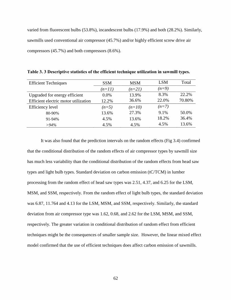
62
varied from fluorescent bulbs (53.8%), incandescent bulbs (17.9%) and both (28.2%). Similarly,
sawmills used conventional air compressor (45.7%) and/or highly efficient screw drive air
compressors (45.7%) and both compressors (8.6%).
Table 3. 3 Descriptive statistics of the efficient technique utilization in sawmill types.
Efficient Techniques SSM MSM LSM Total
(n=11) (n=21) (n=9)
Upgraded for energy efficient 0.0% 13.9% 8.3% 22.2%
Efficient electric motor utilization 12.2% 36.6% 22.0% 70.80%
Efficiency level (n=5) (n=10) (n=7)
80-90% 13.6% 27.3% 9.1% 50.0%
91-94% 4.5% 13.6% 18.2% 36.4%
>94% 4.5% 4.5% 4.5% 13.6%
It was also found that the prediction intervals on the random effects (Fig 3.4) confirmed
that the conditional distribution of the random effects of air compressor types by sawmill size
has much less variability than the conditional distribution of the random effects from head saw
types and light bulb types. Standard deviation on carbon emission (tC/TCM) in lumber
processing from the random effect of head saw types was 2.51, 4.37, and 6.25 for the LSM,
MSM, and SSM, respectively. From the random effect of light bulb types, the standard deviation
was 6.87, 11.764 and 4.13 for the LSM, MSM, and SSM, respectively. Similarly, the standard
deviation from air compressor type was 1.62, 0.68, and 2.62 for the LSM, MSM, and SSM,
respectively. The greater variation in conditional distribution of random effect from efficient
techniques might be the consequences of smaller sample size. However, the linear mixed effect
model confirmed that the use of efficient techniques does affect carbon emission of sawmills.

63
Figure 3. 4 Diagnostic plot of variability of carbon emission (tC) per TCM of lumber
processing by sawmill size at 95% prediction interval on the random effect of efficient
techniques: (a) head saw types, (b) light bulb types, and (c) air compressor types.

64
(b) Avoided carbon emission
An average carbon emission from electricity consumption in sawmills was 10. 07
tC/month. Carbon emission could be reduced by 0.1 - 0.29 tC/month or 1-2.9%, when 2%
electricity saving was achieved using both load and use factor of the machine at 0.6 in sawmills
with a power range from 800 to1600 hp (Figure 3.5a). Increased electricity saving level up to 5%
of existing electricity consumption could increase avoided carbon from 0.25 to 0.73 tC/month or
2.5-7.2%. Greater amount of carbon emission could be avoided when both load and use factors
were used at 0.8 (Figure 3.5b). In this case, avoided carbon emission amount could range from
0.18 to 0.52 tC/month (1.8 -5.2%) at a 2% electricity saving or from 0.45 to 1.3 tC/month (4.5 -
12.9 %) at 5% electricity saving. Likely, in the scenario of the combination of either load factor
at 0.6 or use factor at 0.8 of machine in sawmills could achieve avoided carbon amount from
0.13 to 0.39 tC/month (1.3- 3.9%)%), and 0.34 to 0.98 tC/month (3.4 - 9.7%) at a 2% and 5%
electricity saving level, respectively (Figure 3.5c).
In the base case, greater amount of avoided carbon emission could be achieved from
electricity saving in MSM followed by LSM and SSM. This avoided carbon emission amount
could range from 0.2 to 0.9 tC/TCM (2.13% at SSM -5.14% at MSM) from onsite and offsite
electricity consumption, when 2% to 5% electricity saving was achieved during lumber
production (Figure 3.5d). Though avoided carbon emission amount was less, it could play a
significant role in mitigating greenhouse gaseous impact in Appalachian region in the long run, if
it is accounted for the whole year production level and the total number of sawmills across the
region. This avoided carbon could be instrumental in offsetting carbon emission burden from
wood industries. For large sawmills size, increasing electricity saving could be beneficial in
abating carbon emission as well as adopting carbon cap and trade policy.

65
Figure 3. 5 Avoided C emission using motor master in sawmills: (a) Total Hp at 0.6 load
factor and use factor, (b) Total Hp at 0.8 load factor and use factor (c) Total Hp at 0.6, 0.8
load factor and use factor, and (d) at sawmill size category.
3.3.4 Carbon Balance in Lumber Production
The credit carbon balance accounts for 2.9, 5.5, and 2.8 % of the net debit carbon balance
of lumber (316.5 tC/TCM) at the zero year of lumber production in the SSM, MSM and LSM,
respectively. Effect of this credit carbon balance was not significant in the net debit carbon
balance of lumber at first order of carbon decay up to 100 years (Figure 3.6a). However, it could
affect after the useful life period of 100 years, i.e. beginning of the time period that lumber
66
would be discarded from their use purpose and disposed at landfills. The low credit carbon
balance could be attributed to low electricity consumption by sawmills and it could be increased
when other energy sources consumed were also considered. However, few sawmills reported
consumption of other energy source used in lumber processing such as natural gas, and the total
carbon emission amount from all energy sources involved in the lumber production averaged
13.1 ton/TCM.
Estimated total carbon emission amount from electricity consumption (EC) was 28.5
tC/TCM and it accounts for 9% of the carbon stored in the processed lumber. EC bisects carbon
balance of lumber in 100 years of its useful life period at year 79, where the amount of carbon
remained in lumber at first order of decay rate becomes equivalent to EC (Figure 3.6b). The
payoff period (PP) begins after year 79 and reduced the carbon accountability period of lumber
in its useful life by 21%. Similarly, 35.91 tC/TCM of credit carbon balance generated from all
energy sources (ES) accounted for 11.35 % of the carbon balance in lumber. ES also bisects
carbon balance of lumber at year 67 and shortens carbon accountable period of the lumber
almost by 33 % (Figure 3.6b). Hence, carbon emitted from lumber after the bisected year would
be equivalent to the amount of carbon debt created by credit carbon balance from lumber
processing. The higher the debt carbon balance is, the early PP and consequently lower the
carbon accountability in useful life period of the lumber would be. This PP of credit carbon
would vary depending on the hardwood tree species used for lumber processing because the
carbon content value among tree species differs. Debt carbon from lumber would attribute more
if accounted cumulative carbon emission that occurred from harvesting of timber, transportation
of lumber and energy consumed in lumber used for. Therefore, to neutralize such carbon debt,

67
reforestation of the harvested area should be conducted timely to pay off the credit carbon
balance.
Figure 3. 6 Effect of credit carbon balance in carbon balance of lumber and fraction of
carbon disposition in sawlogs at 100 years period: (a) and (b) carbon balance by carbon
emission level and energy consumption, (c) average sawmill energy consumption, and (d)
electricity consumption (EC) all energy sources (ES).
Lumber processing of 1000 m3 sawlogs contains an average of 680 metric tons of carbon.
This carbon disposition pattern of sawlogs was significantly affected by the generated credit

68
carbon balance. An average credit carbon balance generated from all energy sources in lumber
processing at sawmills only affected the carbon disposition pattern in landfills (Figure 3.6c). The
generated carbon credit balance from only EC affected the period of carbon disposition pattern of
sawlogs and the PP of credit carbon begins either for fraction of carbon in use at last 11 years of
useful life or for fraction of carbon in landfills at first 3 years (Figure 3.6d). Likely, credit carbon
balance from ES also affected the fraction of carbon in use and reduced carbon disposition period
to 76 years (Figure 3.6d). It also affected fraction of carbon disposition period in landfills for
first 3.5 years.
Accounting credit carbon balance against the carbon stored in wood product showed the
similar pattern of shortening useful life period for both lumber at first order of decay (Figure
3.6a and 3.6b) and fraction of carbon disposition pattern in sawlogs (Figure 3.6c and 3.6d).
Though credit carbon balance shortened useful life period of wood products, it tentatively
estimated carbon accountability period of the lumber similar to the half life of solid wood
products in single-family housing (75-80 years) (Skog and Nicholson, 1998; Skog, 2008; Lippke
et al. 2010). When accounted credit carbon balance at year zero of lumber production, it just
lowered the net carbon balance and showed the regular trends of carbon disposition as reported
by Smith et al. (2006). However, deduction of carbon from lumber is not possible at its
production year. Paying off of such generated credit carbon balance from re-growth or
reforestation of the harvested area would not be possible in the same harvest year and
concurrently it would be also augmented by the fuel consumption involved in the artificial
regeneration process. A similar study addressed how to pay off such carbon debt in
Massachusetts (MCCS, 2010), while producing of an equivalent amount of energy from woody
biomass and fossil fuel burning. Almost 9 tons of carbon debt occurred from the utilization of
69
woody biomass energy. It could be recovered in 32 years by forest growth and after the benefit
of burning woody biomass begins to accrue. Therefore, accounting the PP for carbon emission
from wood product processing against the carbon stored in wood product in its useful life period
would be reliable measures to compensate carbon emission amount from energy consumed in
wood processing.
3.3.5 Carbon Flux from lumber processing
More carbon was emitted in the lumber processing mainly from the generated mill
residues. Carbon flux from the use and no use of mill residues was 96.56 tC/TCM as energy
capture, 55.3 tC/TCM as industrial use, 88.51 tC/TCM as farm manure, and 123.8 ton/TCM as
others. The use and no use of mill residues increases the atmospheric carbon level from zero year
of lumber production to 5 years depending on what purposes they are used for (Karjalainen et al.,
2002; Skog, 2008; Zeng, 2008; Sharma, 2010). Carbon flux was also instigated by export of the
lumber. An average of 6.7% of lumber produced was exported and it reduced carbon stock of
lumber production place to 93.3%.
3.3.6 Sensitivity Analysis of Carbon Emission from Lumber Processing
In the base case, the mean carbon emission from electricity consumption would be 24.63
± 0.68 tC/TCM during processing of hardwood lumber in sawmills in the Appalachian region.
The carbon emission from electricity consumption would range from 23.28 to 25.88 tC/TCM
(Figure 3.7a) at 2.5 % and 97.5% quantile distribution, respectively. In SSM, the mean carbon
emission would be 13.73 ± 0.92 tC/TCM ranging from 12.03 to 15.55 tC/TCM (Figure 3.7b) at
2.5% and 97.5% quantile distribution, respectively. For MSM, the mean carbon emission from

70
electricity consumption was 18.68 ± 1.12 tC/TM and ranged from 16.41 to 20.94 tC/TCM
(Figure 3.7c) at 2.5% and 97.5% quantile distribution. Similarly, in LSM, the mean carbon
emission was 12.79 ± 1.24 tC/TCM and varied from 10.36 to 15.20 tC/TCM (Figure 3.7d) at
2.5% and 97.5% quantile distribution.
The upper range of carbon emission predicted in the base case was closer to the carbon
emission estimated from the electricity consumption by CORRIM (Bergman and Bowe, 2008)
and it shortened the carbon accountability period of lumber in a similar manner. The simulated
mean carbon emission amount was greater than the estimated average carbon emission in
sawmills of different size. The observed difference between the simulated mean carbon emission
and the estimated mean carbon emission was due to variability in data and associated uncertainty
of electricity consumption rate at sawmills. The simulated mean carbon emission of each case
lied at 50% quantile distribution whereas the estimated mean carbon emission lied at or below
2.5% quantile distribution. Since uncertainty always associates with the energy source for
electricity generation and equipments used in sawmills, it would be better to use upper range of
the simulated carbon emission (tC/TCM) for sawmill estimate.

71
Figure 3. 7 Probability density plot of carbon emission (tC/TCM) from electricity
consumption in lumber processing: (a) Overall average (b) SSM, (c) MSM, and (d) LSM.

72
3.3.7 Scenario Analysis of Carbon Flux from Lumber Processing
The consequence of cumulative carbon emission from energy sources was observed in
the cumulative carbon balance at the first order of carbon decay in the lumber production cycle
of 100 years. In the base case, the CCFlumber (21.1 tC/TCM) was 57.2 % higher than the
cumulative carbon emission from electricity (13.1 ton/TCM) at sawmills for 100 years of lumber
production (Figure 3.8a). However, the combined carbon flux from the electricity and export did
not affect carbon stored in the produced lumber because the CCFR ranged from 0.12 to 0.42
from year zero to year 100.
The cumulative carbon emission from the total energy consumption and export of lumber
could affect the cumulative carbon balance in lumber (Figure 3.8b). In this case, the CCFR from
the all CCFenergy source consumption (ES) (104.57 GJ/TCM) and CCFexport was 0.19 to 0.77 for
the hardwood lumber production years of 0 -100. Thus, at the end of 100 years of production
period, only 23% of the CCBlumber would be available to account as the net debit carbon balance.
Therefore, a great amount of carbon emission would affect the CCBlumber production period and it
would also discount such credit carbon balance at later years of the wood product life.
When 25% of the carbon emission from all energy source consumption was reduced, the
CCFR would range from 0.16 at zero years to 0.65 at 100 years (Figure 3.8c). In this situation,
45% of the carbon in the lumber would be available to account as net CCBlumber at 100 years.
Similarly, if reducing 50% of carbon emission from all energy source consumption (Figure 3.8d),
it could have the similar effect as carbon flux created from electricity and export by sawmills
(Figure 3.8a). But the CCFR would range from 0.13 to 0.53. Thus, either reducing carbon
emission/energy consumption rate or decreasing export of the lumber would help increase
accountability of carbon balance in the lumber production for a long time period. Energy

73
consumption could be reduced by installing a waste oil burner for burning the waste oil to heat
the plant and office areas. It saves the waste oil disposal cost and reduces the potential of a
demining from spill and also less consumption of natural energy. But the waste oil installation
factor depends on the quantity of waste oil generated by sawmill.
Figure 3. 8 Atmospheric carbon fluxes from hardwood lumber processing in 100 years:
(a) average electricity consumption at sawmills (b) all energy source consumption, (c) 25%
reduction in all energy source consumption, and (d) 50% reduction in all energy source
consumption.

74
3.3.8 Carbon Emission under Different Energy Sources
Since a great amount of electricity is required for lumber processing (607.2 GJ/TCM,
Bergman and Bowe, 2008), it increases the atmospheric carbon level significantly. Generating
such amount of electricity from natural gas would emit carbon equivalent to an average carbon
emission level from the current electricity generation from the mixed sources in the Appalachian
region (Figure 3.9a). Carbon emission from single source of electricity generation such as fossil
fuel would be greater followed by coal. Therefore, the electricity generated from an appropriate
mixture of energy sources could help avoid certain amount of credit carbon balance.
In figure (3.9b), the base case represents electricity generation from the mixed energy
sources in central Appalachian region, scenario 1 represents RFC WEST, and scenario 2
represents RFC EAST, and scenario 3 NYUP. The credit carbon balance was 30.92 tC/TCM,
29.5 tC/TCM, 27.2 tC/TCM, and 32.8 tC/TCM for the base case, scenario 1, scenario 2 and
scenario 3 respectively (Figure 3.9b). Scenario 2 would create less credit carbon balance than
scenario 1 and scenario 3, and base case. Though in scenario 3, coal source shared less
percentage of electricity than other scenarios, the higher carbon content value per unit of coal
attribute to the greater amount of credit carbon balance in the represented region. It could be
coupled from the variation in calorific value of coal and oil though these shared greater
percentage of electricity generation than in other scenarios. Though coal shared higher
percentage of electricity generation in the scenario 1 and 2, the lower value of average carbon
content per unit of electricity generation in the represented regions created less credit carbon
balance. Eventually, the credit carbon balance would have less affect on the carbon balance from
lumber production. However, coal is the major source of electricity generation supplemented by
gas and these energy sources usually have higher carbon coefficient value per unit of electricity.

75
Thus carbon credit per unit of lumber processing would vary depending on the electricity supply
sources and their mixed ratio.
Figure 3. 9 Carbon emissions from electricity generation during hardwood lumber
processing using: (a) single energy sources and current average, and (b) mixed energy
sources.
Note: Carbon emission from energy sources is calculated based at their higher heating values
and the average carbon dioxide emission is based on eGrid (US EPA 2010b), CO2: Fossil fuel =
0.851 kg/kWh; Coal = 0.713 kg/kWh; Oil, 0.358 kg/kWh;, Gas = 0.556 kg/kWh;, and Current =
0.62 kg/kWh.

76
3.4. Conclusions
Carbon emission from electricity consumption while per unit of processed lumber vary
depending on sawmill size. This variation would be coupled to electricity generation sources and
available equipment at sawmills while per unit processed lumber. The random mixed effect of
the available equipments such as head saws types, light bulb types and air compressors types also
fluctuate the credit carbon balance of a sawmill. Such carbon emission could be avoided to some
extent if energy efficient motors and equipment were used, which would be beneficial in abating
carbon credit balance. Although carbon stored in produced lumber increases carbon stock of the
wood carbon pool and magnifies humans‘ carbon mitigation efforts, carbon flux occurs due to
significant wood loss during sawmill processing. Not all carbon loss from mill residues would be
immediately recaptured as an energy source and released into the atmosphere. Mill residue used
for either for industrial or mulching and farm bedding use would help to store significant amount
wood carbon from being emitted for the time period as short lived wood product does.
Carbon balance in lumber would be affected by the credit carbon generated during its
processing. It could also impair the carbon accountability period of lumber during its useful life.
Carbon disposition pattern of sawlogs would also be greatly affected by this credit carbon
balance. Carbon flux from the export of lumber also decreases the carbon accountability of the
cumulative lumber production in years. The greater the carbon flux ratio from energy and export,
the lower the carbon accountability of the produced lumber would be. Carbon emission from
electricity consumption could be minimized by using energy sources that have a lower carbon
coefficient. Thus, appropriate mixed energy sources in the region would be helpful to minimize
carbon emission from electricity consumption at sawmills.

77
References
Apps, M. J., Kurz,W. A., Beukema, S. J. and Bhatti, J.S. 1999. Carbon budget of the Canadian
forest product sector, Env. Sci. Policy 2, 25–41.
Bergman, R. D. and Bowe, S. C. 2008. Life-Cycle Inventory of Hardwood Lumber
Manufacturingin the Northeast and North Central United States, CORRIM: Phase II Final
Report Module C, p 1-48.
Blasing, T. J., Broniak, C. T. and Marland, G. 2005., The annual cycle of fossil-fuel carbon
dioxide emissions in the United States. Tellus B, 57: 107–115
Birdsey, R. A. 2006. Carbon accounting rules and guidelines for the United States Forest Sector.
J. Environ. Qual., Vol. 35, 2006, 1518-1524.
Brown, S., Lim, B. and Schlamadinger, B.1998. Evaluating approaches for estimating net
emissions of carbon dioxide from forest harvesting and wood products. Meeting Report,
IPCC/OECD/IEA Programme on National Greenhouse Gas Inventories, Dakar, Senegal,
5-7 May 1998. pp. 20.
Dias, A. C., Louro, M., Arroja, L., and Capela I .2005. The contribution of wood products to
carbon sequestration in Portugal.2005.- Ann. For. Sci. 62 (8) 903-909 .
Gopalakrishan, B., Winn, G., Chauhari, S., Bhadra, S., and Sundaramoorthy, S. K., 2008.
Integrated assessment report focusing on IOF WV Priorities. Wood industry assistance
program. Supported by West Virginia development office-Energy efficiency program.
Gower, S. T. 2003. Patterns and mechanisms of the forest carbon cycle. Ann. Rev. Environ.
Resour. 28, 169–204.

78
Harmon, M. E., Harmon, J. E., Ferrell, W. K., and Brooks, D. 1994. ‗Modeling carbon stores in
Oregon and Washington forest products: 1900–1992‘, Climatic Change 33, 521–550
Ingerson, A. 2009. Wood products and carbon storage: Can increased production help solve the
climate crisis? Washington, D.C.: The Wilderness Society pg 6.
IPCC,2003. Intergovernmental Panel on Climate Change Estimation, Reporting and
accounting of harvested wood products – Technical Paper. UNFCCC paper. pp 44.
Karjalainen, T., Pussinen, A., Liski, J., Nabuurs, G.J., Erhard, M., Eggers, T., Sonntag, M.,
Mohren, F. 2002. An approach towards an estimate of the impact of forest management
and climate change on the European forest sector budget: Germany as a case study.
Forest Ecology and Management 162:87-103
Kurz, W. A., Apps, M. J., Webb, T. M. & McNamee, P. J. 1992. The carbon budget of the
canadian forest sector: Phase I, Information Report NOR-X-326, Forestry Canada,
Northwest Region, Forestry Centre, pp. 93
Lippke, B., Wilson, J., Meil, J. and Taylor, A. 2010. Characterizing the importance of carbon
stored in wood products. CORRIM special Issue, March 2010, V.42, 5-14
MCCS [Manomet Center for Conservation Sciences]. 2010. Massachusetts biomass
sustainability and carbon policy study: Report to the Commonwealth of Massachusetts
Department of Energy Resources. Walker, T. (Ed.). Contributors: Cardellichio, P.,
Colnes, A., Gunn, J., Kittler, B., Perschel, R., Recchia, C., Saah, D., and Walker, T.
Natural Capital Initiative Report NCI-2010-03. Brunswick, Maine. pp.182.
Micales, J.A. and Skog, K.E. 1997. The decomposition of forest products in landfills. Int.
biodeterior. Biodegard. 39:145-158.

79
NREL [National Renewable Energy Laboratory].2010. Life cycle inventory database,
http://www.nrel.gov/lci/database/, accessed December 20, 2011.
Perlack, R.D., Wright, L.L., Turhollow, A.F., Graham, R.L., Stokes, B.J., Erbach., D.C. 2005.
Biomass as feedstock for a bioenergy and bioproducts industry: The technical feasibility
of a billion-ton annual supply. DOE/USDA Tech. Rep. DOE/GO-102005–2135. USDOE,
Office of Scientific & Technical Information, Oak Ridge, TN, p. 78.
Pingoud, K., Savolainen, I., and Seppala ,H. 1996. Greenhouse impact of the Finnish forest
sector including forest products and waste management, Ambio 25(5), 318–326.
Pingoud,K., Perälä, A. L., and Pussinen, A. 2001. Carbon dynamics in wood products.
Mitigation and Adaptation Strategies for Global Change 2001, 6: 91–111.
Puettmann, M. E., Bergman, R., Hubbard, S., Johnson, L., Lippke, B., Oneil, E. and Wagner, F.
G. 2010. Cradle to gate life cycle inventory of us products production: CORRIM phase 1
and phase 2 products. CORRIM special issue, March 2010, V.42, 15-28.
Row, C. and Phelps, R.B. 1996. Wood carbon flows and storage after timber harvest. Forests and
Global Change Vol. 2: Forest management opportunities for mitigating carbon emissions,
Sampson, R.N., Hair, D., eds. American Forests. Washington, D.C. 27-58.
Saud, P. 2011. Analysis of forest carbon balance in central Appalachia region. Master Thesis
(draft) submitting to Division of Forestry, West Virginia University.
Schlamandinger, B. J., Spitzer, G., Kohlmaier, H. and Deke, M. L. 1995, Carbon balance of
bioenergy from logging residues. Biomass and Bioenergy 8(4), 221-234 (1995).
Sharma, B.D. 2010. Modeling of forest harvest scheduling and terrestrial carbon sequestration.
Dissertation Submitted for the degree of Doctor of Philosophy in Forest Resource
Science, West Virginia University, 2010, 1-159.

80
Skog, K .E. and Nicholson,G .A. 1998. Carbon cycling through wood products: The role of wood
and paper products in carbon sequestration. Forest Products Journal 48:75-83
Skog, K .E., Pingoud, K., Smith, J. E. 2004. A method country can use to estimate changes in
carbon stored in harvested wood products and the uncertainty of such estimates.
Environmental Management. 33(Suppl. 1): S65-S73.
Skog, K. E. 2008. Sequestration of carbon in harvested wood products for the United States.
Forest product journal. Vol 58. No.6 (June 2008): pages 56-72.
Siau, J. F. 1984. Transport processes in wood. Springer-Verlag, NewYork. 245p
Smith, J. E., Heath ,L, S,, Skog, K .E., Birdsey, R. A. 2006. Methods for calculating forest
ecosystem and harvested carbon with standard estimates for forest types of the United
States. Gen. Tech. Rep. NE-343. Newtown Square, PA: U.S. Department of Agriculture,
Forest Service, Northeastern Research Station. 216 p.
USDA FS. 2010. Timber Product Output (TPO) Reports November 04, 2010
http://srsfia2.fs.fed.us/php/tpo_2009/tpo_rpa_int2.php, accessed January 20, 2011
USDOE [US Department of Energy]. 2010. Energy Efficiency and Renewable Energy, Industrial
Technologies Program, Release Date: September 21, 2010,
(http://www1.eere.energy.gov/industry/bestpractices/software_motormaster.html)
accessed February 15, 2011.
USEIA [US Energy Information Administration].2010. Average retail price of electricity to
ultimate customers, Report Released: November 2010
http://www.eia.doe.gov/cneaf/electricity/esr/table5.html. (Accessed Jan 25, 2011)

81
US EIA 2011. US Energy Information, Independent Statistics and Analysis, Voluntary reporting
of greenhouse gases program fuel emission coefficients
(http://www.eia.doe.gov/oiaf/1605/coefficients.html) accessed March 2, 2011
USEPA [US Environmental Protection Agency]. 2005. Emission Fact, Office of Transportation
and Air Quality, EPA420-F-05-001 February 2005. pp 2.
USEPA [US Environmental Protection Agency]. 2010a. Inventory of U.S. Greenhouse Gas
Emissions and Sink: 1990-2008. April 15, 2010 U.S. Environmental Protection Agency,
Washington, DC, pg 1-407
USEPA[US Environmental Protection Agency ]. 2010b. Environmental Protection Agency,
Emissions & Generation Resource Integrated Database (eGRID)
http://cfpub.epa.gov/egridweb/view.cfm, accessed December 28, 2010.
Werner, F., Taverna, R., Hofer, P., Richter, K. 2005. Carbon pools and substitution effects of an
increased use of wood in buildings in Switzerland: first estimates. Annals of For. Sci. 62,
889-902.
White, M. K., Gower, S. T., and Ahl, D. E. 2005. Life cycle inventories of roundwood
production in northern Wisconsin: Inputs into an industrial forest carbon budget Forest
Ecology and Management 219 (2005) 13–28
Wilson, J.B. and Dancer, E. R. 2005. Gate to gate life cycle inventory of laminated veneer
lumber production. Wood and Fiber Science, 37 CORRIM Special Issue, 2005, pp 114-
127.
Winjum, J. K., Brown, S. and Schlamadinger, B. 1998. Forest harvests and wood products:
sources and sinks of atmospheric carbon dioxide. Forest Science 44:272-284.
Zeng, N. 2008. Carbon sequestration via wood burial.Carbon Balance and Management 3:1-12

82
4. SUMMARY
Inclusion of parameters such as carbon loss from dead trees, forest fire along with timber
removal and forest growth rate is essential to estimate future carbon balance of the timberland.
The lower harvesting intensity of the existing timber stock volume, small amount of carbon
removal from small fire and limited dead trees do not significantly affect the future forest carbon
stock per hectare. However, the observed high mortality rate of trees could be a major factor to
limit the sustainable increase of forest carbon stock in West Virginia. Increasing timber demand
could be met with slight increases in existing harvesting intensity and making constant
harvesting intensity for certain consecutive years. This would help to lengthen the rotation age of
natural mixed hardwood forest and also increase forest carbon stock. Eventually, this strategy
would employ the sustainable forest management practice and also undermine the effect of
carbon emissions from fossil fuel consumption due to timber harvesting and processing.
Natural regeneration in forests, as applicable in the Appalachian region, entails no fossil
fuel consumption in seedling production and plantation and thus results in zero carbon emission
from regeneration process. Carbon emission from mechanized harvesting system and manual
harvesting system did not differ significantly. The variations associated with the machine
productivity and the tree size would influence the carbon emission level from harvesting systems
to some extent. However, these variations would be significant when considering topographic
factors attributed to the harvested area. In harvesting and residue extraction, the hauling process
has a greater effect on carbon emission than other operational procedures. Though carbon
emissions from fossil fuel consumption from harvesting systems are considerably lower than the
carbon stored in harvested timber and logging residue, the forest carbon displacement rate would
varies with forest group types, road types, hauling truck types, and payload sizes. Forest type
83
having lower carbon content per unit of harvested volume and hauling smaller payload would
increase forest carbon displacement rate. In hauling, the distance travelled on gravel road and
paved road, and payload variation of harvested timber dimensions would determine the
magnitude of carbon emission. Therefore, hauling distance and truck payload size indicate a
greater uncertainty of carbon emissions level, which increases the forest carbon displacement
rate and reduce the accountability of carbon balance in harvested timber.
Different levels of credit carbon balance are generated from carbon emitted from
electricity consumption depending on operation hours and lumber processing quantity of
different sawmills sizes. This variation is attributed to electricity generated from different energy
sources. Similarly it is also attributed to the available equipment and its energy efficiency level at
sawmills while processing per unit of lumber. For example, different head saws, light bulbs and
air compressors used in sawmills fluctuated the degree of credit carbon balance. Such generated
credit carbon balance could be lowered to some extent if using energy efficient motors and
equipment. During lumber processing, a substantial amount of carbon emission occurs due to
wood loss as mill residue other than carbon stored in the processed lumber products. Not all
carbon loss from mill residues, such as chips and sawdust, would be immediately recaptured as
an energy source (e.g. heat/fuel source) in sawmills. The amount of mill residue that used for
mulching and farm bedding would be significant to lengthen carbon release time period.
The generated credit carbon balance during lumber processing could impair the carbon
accountability period of lumber during its useful life period. Carbon disposition pattern of
sawlogs would also be greatly affected by this credit carbon balance. The greater the credit
carbon balance, the shorter the debt payoff period would be, and the shorter the carbon
accountability period of wood product in its useful life period. This payoff period could vary

84
depending on hardwood tree species. Carbon emission from energy consumption and carbon loss
from export of hardwood lumber create carbon flux in the wood carbon stock. Such cumulative
carbon flux from energy consumption and lumber export would reduce the accountability of
carbon balance during lumber production in years. The greater the cumulative carbon flux ratio,
the lower the carbon balance accounted from the lumber production. Such carbon flux ratio
could be minimized by reducing energy consumption rate in lumber processing. One of the
feasible options to reduce energy consumption is to install a waste oil burner to heat the plant
and office areas and it also saves waste oil disposal cost depending on the quantity of waste oil
generated in sawmill. Additionally, the use of different energy sources that has lower carbon
coefficient value would be advantageous to supply the required amount of electricity to process
per unit of lumber. An appropriate mixed energy source in the region would be helpful to
minimize credit carbon balance from electricity consumption at sawmills.