LiDAR Remote Sensing for

Natural Resource Management

Paul TreitzDepartment of Geography, Queen’s University

Murray WoodsOntario Ministry of Natural Resources

Kevin LimLim Geomatics Inc.

Valerie ThomasDepartment of Forestry, Virginia Tech

Harry McCaugheyDepartment of Geography, Queen’s University

Active remote sensing

system

Up to 200,000 pulses of

laser light per second

Pulses strike the

objects/surface of the

earth and with each pulse

the sensor receives a

measurement of the time

and angle of each return.

As the laser pulse strikes a

surface, it will produce

range and intensity

measurements (multiple).

Light Detection and Ranging (LiDAR)

Digital Surface Model (DSM)

Digital Terrain Model (DTM)

Canopy Height Model (CHM)

Canopy Height Models

LiDAR’s Contribution to Forest Inventory

Detailed Surface Models– Digital Surface Models

– Digital Terrain Models

– Canopy Height Models

Detailed Digital Terrain Model– Supporting

Identifying surficial geology

Hydrological modelling

Wetland identification

Predictive ecosystem mapping

Operational considerations– road construction

– skid trail layout

– water crossings

Valu

e A

dde

d

Road layout using least cost path analysis

techniques.

Origin

Destination

Slope

DEM 2m

Profile from DEM

55

Swan Lake Research Forest tolerant hardwood forest no–

harvest/single tree selection.

Petawawa Research Forest plantation, natural unharvested, and

silviculturally treated conifer stands.

Nippising Forest Sites young yellow birch

red oak conditions; and

natural white pine conditions

Predicting Forest Inventory Variables

Woods, M., K. Lim, and P. Treitz. 2008. Predicting forest stand variables from LiDAR data in

the Great Lakes St. Lawrence Forest of Ontario, Forestry Chronicle, 84(6): 827-839.

6

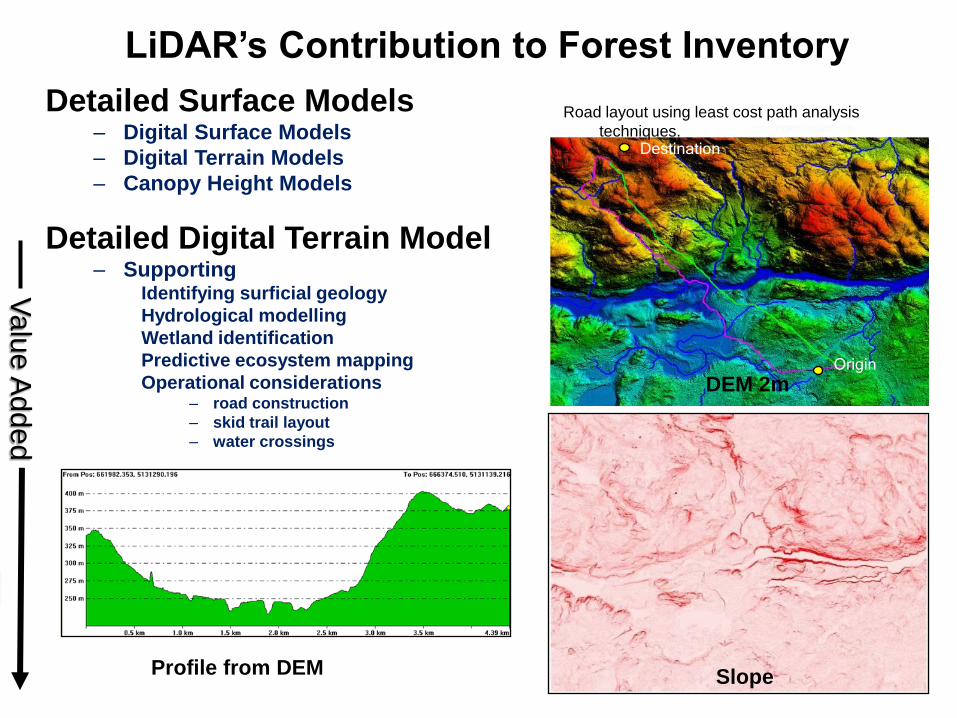
Forest Stand Characteristics

7

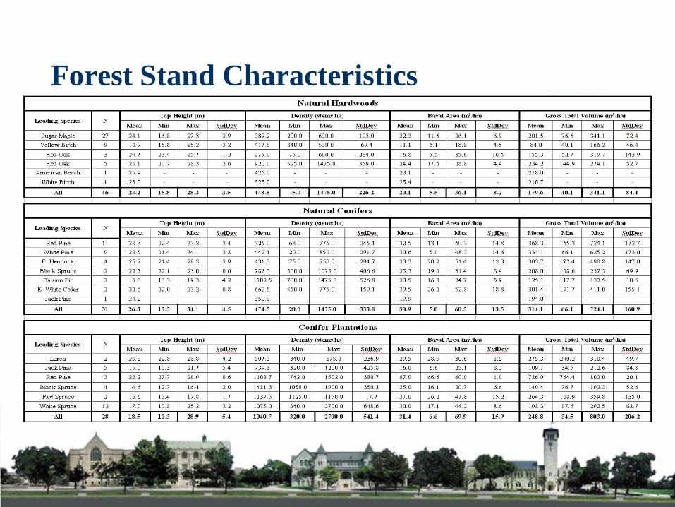
Top Height (m)(TOPHT) Calculated as the average of the largest 100 stems per hectare.

Average Height (m)(AVGHT) Calculated as the average height of all trees.

Density (stems ha-1)(DENSITY) Number of live trees.

Quadratic Mean Diameter (cm)(QMDBH)

Basal Area (m2 ha-1)(SUMBA) DBH2 * 0.00007854

Gross Total Volume (m3 ha-1)(SUMGTV) Honer et al. (1983) equations.

7

nDBH 2

Forest Variables

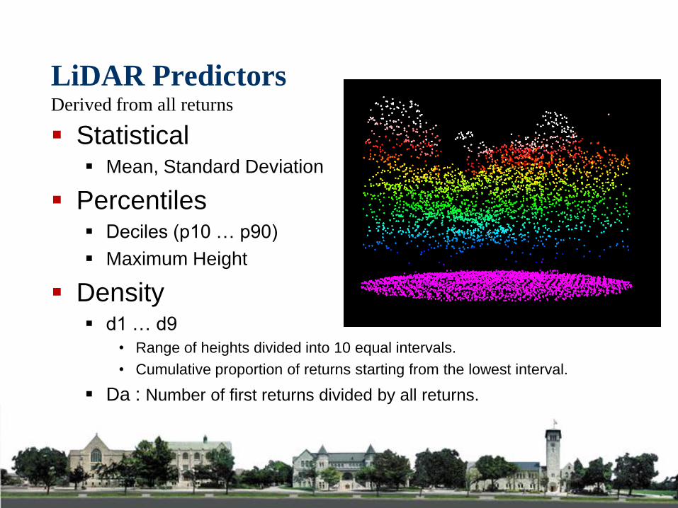
LiDAR PredictorsDerived from all returns

Statistical Mean, Standard Deviation

Percentiles Deciles (p10 … p90)

Maximum Height

Density d1 … d9

• Range of heights divided into 10 equal intervals.

• Cumulative proportion of returns starting from the lowest interval.

Da : Number of first returns divided by all returns.

0

5

10

15

20

25

30

4.2966e+5

4.2967e+5

4.2968e+5

4.2969e+54.2970e+5

4.2971e+5

4.681400e+64.681405e+64.681410e+64.681415e+64.681420e+64.681425e+64.681430e+64.681435e+6

Z D

ata

X D

ata

Y Data

ACFL

P0

hei

ght

1

q(ht)

q(ht)

q(ht)

q(ht)

q(ht)

q(ht)

q(ht)

q(ht)

q(ht)

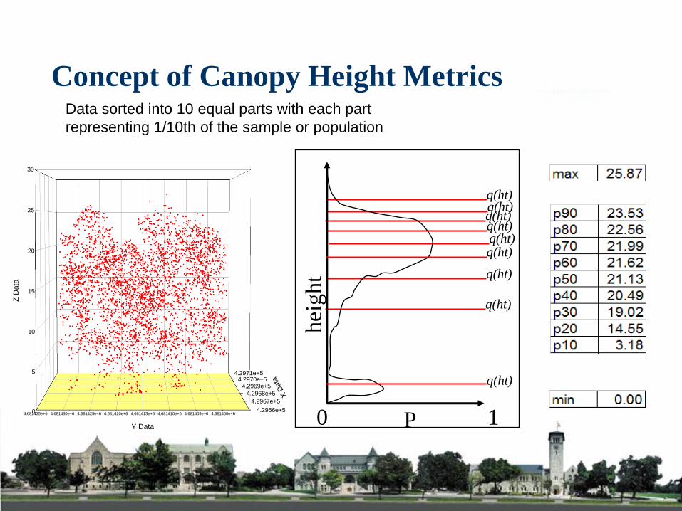
Data sorted into 10 equal parts with each part

representing 1/10th of the sample or population

Concept of Canopy Height Metrics

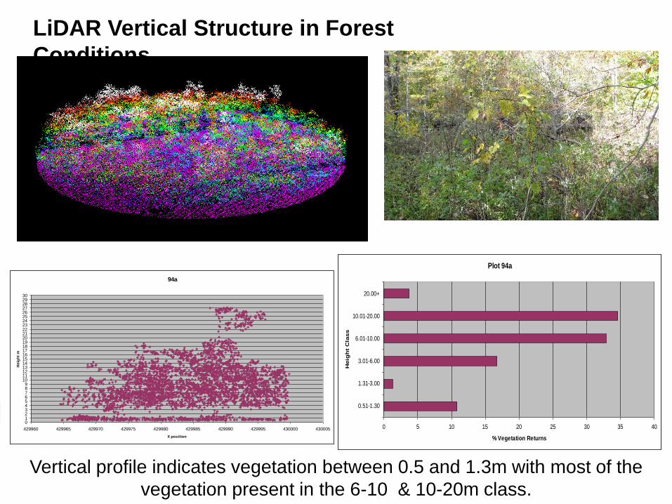
LiDAR Vertical Structure in Forest

Conditions

Vertical profile indicates vegetation between 0.5 and 1.3m with most of the

vegetation present in the 6-10 & 10-20m class.

Plot 94a

0 5 10 15 20 25 30 35 40

0.51-1.30

1.31-3.00

3.01-6.00

6.01-10.00

10.01-20.00

20.00+

Heig

ht

Cla

ss

% Vegetation Returns

94a

0123456789

101112131415161718192021222324252627282930

429960 429965 429970 429975 429980 429985 429990 429995 430000 430005

X position

Heig

ht

m

11

Best Subsets Regression A model-building technique that identifies subsets of

variables that best predict responses on a dependent variable by linear or non-linear regression.

Model Diagnosis Test for Normality: Shapiro-Wilks Test

Test for Homoschedasticity: Modified Levene’s Test

Multicollinearity: Variance Inflation Factors (VIF) < 10

Natural Logarithm Transformation

Validation PRESS Procedure

11

Statistical Analysis

Regression Models: Natural Hardwoods

Variable R2 p RMSE

(%)

PRESS RMSE

(%)

SUMBA (m2/ha) 0.82 < 0.001 3.46

(17.2)

3.99

(19.9)

SUMGTV (m3/ha) 0.90 < 0.001 39.35

(21.9)

52.03

(29.0)

DENSITY

(stems/ha)

0.77 < 0.001 196.03

(43.7)

214.98

(47.9)

QMDBH (cm) 0.82 < 0.001 3.07

(12.4)

4.17

(16.8)

AVGHT (m) 0.87 < 0.001 1.10

(5.7)

1.25

(6.4)

TOPHT (m) 0.96 < 0.001 0.80

(3.5)

0.89

(3.8)

Canopy Height Model (CHM)

1414

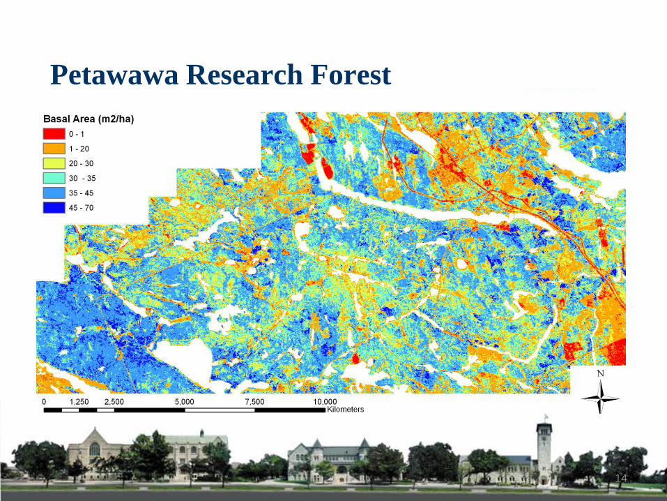
Petawawa Research Forest

Goal:

To develop standards for LiDAR data

acquisition in support of modelling forest

inventory variables.

Objective(s):

Examine the impact of changes in pulse

densities on modelling forest inventory

variables.

LiDAR Data Acquisition Standards

Natural Tolerant Hardwood Natural Conifer Shelterwood Conifer Plantation

RGB Image

0.5

pulses/m2

3 pulses/m2

LiDAR Data Acquisition Standards

Variable Decimation Level 0 Decimation Level 1 Decimation Level 2

R2 RMSE(%)

R2 RMSE(%)

R2 RMSE(%)

SUMBA(m2/ha)

.49 2.7(10.6)

.49 2.7(10.7)

.58 2.4(9.7)

SUMGTV(m3/ha)

.59 25.4(11.2)

.60 24.9(11.0)

.61 24.8(11.0)

DENSITY(stems/ha)

.84 42.8(10.5)

.86 39.8(9.8)

.83 43.7(10.7)

QMDBH(cm)

.69 2.0(7.3)

.72 1.9(7.0)

.70 2.0(7.1)

AVGHT(m)

.84 0.6(3.4)

.84 0.6(3.4)

.85 0.6(3.2)

TOPHT(m)

.82 0.7(3.0)

.85 0.7(2.8)

.86 0.7(2.7)

SUMBIO(kg/ha)

.46 24,795(12.6)

.50 23,811(12.1)

.58 23,811(12.1)

Swan Lake – Tolerant HardwoodsCurrent Status

Preliminary Results

Variable Decimation Level 0 Decimation Level 1 Decimation Level 2

R2 RMSE(%)

R2 RMSE(%)

R2 RMSE(%)

SUMBA(m2/ha)

.89 4.8(13.3)

.89 4.7(13.2)

.88 4.9(13.7)

SUMGTV(m3/ha)

.93 56.1(13.4)

.94 51.2(12.3)

.92 60.0(14.4)

DENSITY(stems/ha)

.74 207.8(34.7)

.72 214.9(35.8)

.68 226.9(37.8)

QMDBH(cm)

.87 3.9(12.7)

.86 4.0(12.9)

.87 3.8(12.3)

AVGHT(m)

.94 1.3(5.7)

.94 1.3(6.0)

.94 1.3(5.7)

TOPHT(m)

.95 1.2(4.4)

.95 1.2(4.5)

.94 1.3(4.7)

SUMBIO(kg/ha)

.74 29,818(21.0)

.76 28,743(20.3)

,78 27,572(19.4)

Current StatusPetawawa Research Forest – Great Lakes

Pine

Preliminary Results

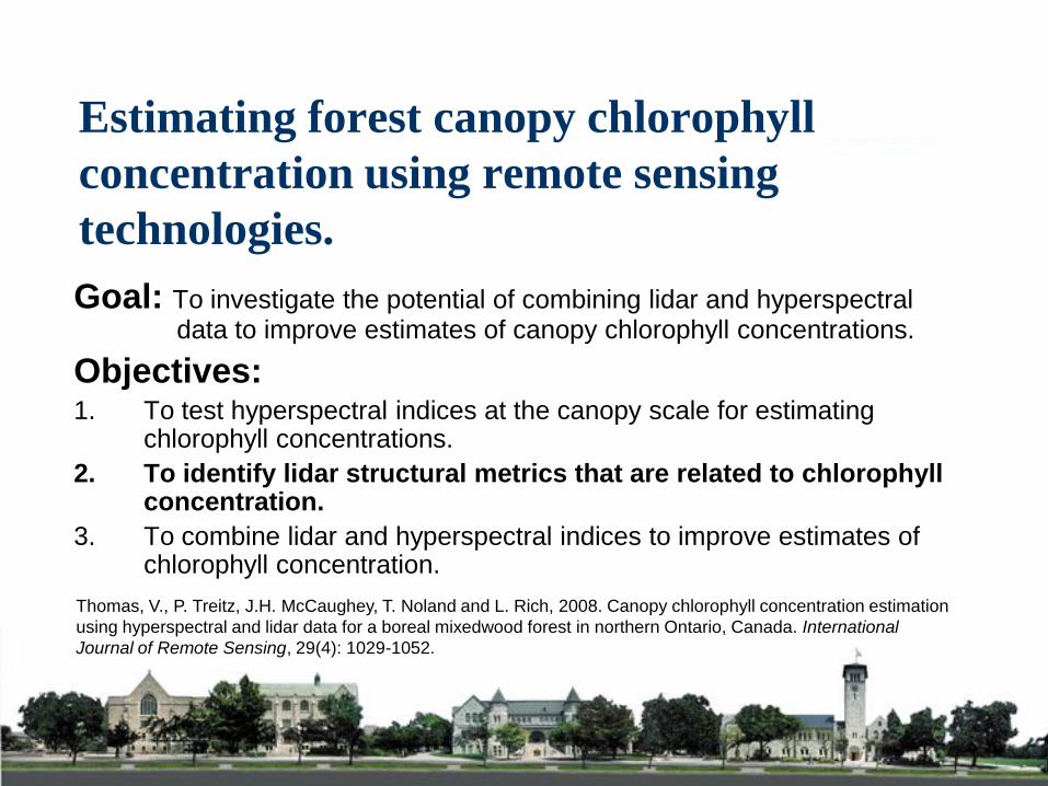
Goal: To investigate the potential of combining lidar and hyperspectraldata to improve estimates of canopy chlorophyll concentrations.

Objectives:1. To test hyperspectral indices at the canopy scale for estimating

chlorophyll concentrations.

2. To identify lidar structural metrics that are related to chlorophyll concentration.

3. To combine lidar and hyperspectral indices to improve estimates of chlorophyll concentration.

Estimating forest canopy chlorophyll

concentration using remote sensing

technologies.

Thomas, V., P. Treitz, J.H. McCaughey, T. Noland and L. Rich, 2008. Canopy chlorophyll concentration estimation

using hyperspectral and lidar data for a boreal mixedwood forest in northern Ontario, Canada. International

Journal of Remote Sensing, 29(4): 1029-1052.

Study Area

Groundhog River Fluxnet Site (GRFS)

Timmins, Ontario, Canada

Lat/Long: 48 °N, 82 °W

Boreal Mixedwood Site

Trembling Aspen (TA)

White Birch (WB)

White Spruce (WS)

Black Spruce (BS)

Balsam Fir (BF)

White Cedar (C)

Plots11.3 m radius; 400 m2

Height, dbh, crown width

Calibration Plots (24)

Validation Plots (9)

Results – Lidar Data

Lidar first return point clouds for: open black spruce canopy;

and trembling aspen canopy with balsam fir understory.

Results – Lidar Data

Relationships between average total leaf

chlorophyll concentration (a+b) and mean

lidar height above ground during August

2003 (lidar data) and August 2004 (leaf

chlorophyll concentration).

Groundhog River Flux Site,

August 2004, maps of mean of

25th percentile of lidar heights

above ground (m).

Results – Hyperspectral / Lidar

Integrated lidar-hyperspectral model

(lidar25/DCI) for average leaf total

chlorophyll (a+b).

Map of total chlorophyll (a+b)

(μg/cm2) derived from the integrated

lidar-hyperspectral model.

Acknowledgements