Embed Size (px)
Citation preview
8/3/2019 Liam Thomas Watson- Knots, Tangles and Braid Actions
http://slidepdf.com/reader/full/liam-thomas-watson-knots-tangles-and-braid-actions 1/82
KNOTS, TANGLES AND BRAID ACTIONS
by
LIAM THOMAS WATSON
B.Sc. The University of British Columbia
A THESIS SUBMITTED IN PARTIAL FULFILLMENT OFTHE REQUIREMENTS FOR THE DEGREE OF
MASTER OF SCIENCE
in
THE FACULTY OF GRADUATE STUDIES
Department of Mathematics
We accept this thesis as conformingto the required standard
. . . . . . . . . . . . . . . . . . . . . . . . . . . . . . . . . . . . .
. . . . . . . . . . . . . . . . . . . . . . . . . . . . . . . . . . . . .
THE UNIVERSITY OF BRITISH COLUMBIA
October 2004
c Liam Thomas Watson, 2004

8/3/2019 Liam Thomas Watson- Knots, Tangles and Braid Actions
http://slidepdf.com/reader/full/liam-thomas-watson-knots-tangles-and-braid-actions 2/82
In presenting this thesis in partial fulfillment of the requirements for an advanced
degree at the University of British Columbia, I agree that the Library shall make
it freely available for reference and study. I further agree that p ermission for ex-
tensive copying of this thesis for scholarly purposes may be granted by the head of
my department or by his or her representatives. It is understood that copying or
publication of this thesis for financial gain shall not be allowed without my written
permission.
(Signature)
Department of MathematicsThe University of British ColumbiaVancouver, Canada
Date
8/3/2019 Liam Thomas Watson- Knots, Tangles and Braid Actions
http://slidepdf.com/reader/full/liam-thomas-watson-knots-tangles-and-braid-actions 3/82
Abstract
Recent work of Eliahou, Kauffmann and Thistlethwaite suggests the use of braid actions to alter a link diagram without changing the Jones polynomial.This technique produces non-trivial links (of two or more components) havingthe same Jones polynomial as the unlink. In this paper, examples of distinctknots that can not be distinguished by the Jones polynomial are constructedby way of braid actions. Moreover, it is shown in general that pairs of knots
obtained in this way are not Conway mutants, hence this technique providesnew perspective on the Jones polynomial, with a view to an important (andunanswered) question: Does the Jones polynomial detect the unknot?
ii
8/3/2019 Liam Thomas Watson- Knots, Tangles and Braid Actions
http://slidepdf.com/reader/full/liam-thomas-watson-knots-tangles-and-braid-actions 4/82
Table of Contents
Abstract ii
Table of Contents iii
List of Figures v
Acknowledgement vii
Chapter 1. Introduction 1
Chapter 2. Knots, Links and Braids 3
2.1 Knots and Links . . . . . . . . . . . . . . . . . . . . . . . . . . . . . . . . . . . . . . . . . . . . . . . . . 32.2 Braids . . . . . . . . . . . . . . . . . . . . . . . . . . . . . . . . . . . . . . . . . . . . . . . . . . . . . . . . . . . 5
Chapter 3. Polynomials 8
3.1 The Jones Polynomial . . . . . . . . . . . . . . . . . . . . . . . . . . . . . . . . . . . . . . . . . . . 83.2 The Alexander Polynomial . . . . . . . . . . . . . . . . . . . . . . . . . . . . . . . . . . . . . . . 9
3.3 The HOMFLY Polynomial . . . . . . . . . . . . . . . . . . . . . . . . . . . . . . . . . . . . . . 13
Chapter 4. Tangles and Linear Maps 21
4.1 Conway Tangles . . . . . . . . . . . . . . . . . . . . . . . . . . . . . . . . . . . . . . . . . . . . . . . . 214.2 Conway Mutation . . . . . . . . . . . . . . . . . . . . . . . . . . . . . . . . . . . . . . . . . . . . . . 254.3 The Skein Module . . . . . . . . . . . . . . . . . . . . . . . . . . . . . . . . . . . . . . . . . . . . . . 274.4 Linear Maps . . . . . . . . . . . . . . . . . . . . . . . . . . . . . . . . . . . . . . . . . . . . . . . . . . . . 314.5 Braid Actions . . . . . . . . . . . . . . . . . . . . . . . . . . . . . . . . . . . . . . . . . . . . . . . . . . 32
Chapter 5. Kanenobu Knots 37
5.1 Construction . . . . . . . . . . . . . . . . . . . . . . . . . . . . . . . . . . . . . . . . . . . . . . . . . . . 37
5.2 Basic Examples . . . . . . . . . . . . . . . . . . . . . . . . . . . . . . . . . . . . . . . . . . . . . . . . 415.3 Main Theorem . . . . . . . . . . . . . . . . . . . . . . . . . . . . . . . . . . . . . . . . . . . . . . . . . 425.4 Examples . . . . . . . . . . . . . . . . . . . . . . . . . . . . . . . . . . . . . . . . . . . . . . . . . . . . . . 465.5 Generalisation . . . . . . . . . . . . . . . . . . . . . . . . . . . . . . . . . . . . . . . . . . . . . . . . . . 505.6 More Examples . . . . . . . . . . . . . . . . . . . . . . . . . . . . . . . . . . . . . . . . . . . . . . . . . 535.7 Observations . . . . . . . . . . . . . . . . . . . . . . . . . . . . . . . . . . . . . . . . . . . . . . . . . . . 59
iii
8/3/2019 Liam Thomas Watson- Knots, Tangles and Braid Actions
http://slidepdf.com/reader/full/liam-thomas-watson-knots-tangles-and-braid-actions 5/82
Table of Contents iv
Chapter 6. Thistlethwaite Links 62
6.1 Construction . . . . . . . . . . . . . . . . . . . . . . . . . . . . . . . . . . . . . . . . . . . . . . . . . . . 626.2 Some 2-component examples . . . . . . . . . . . . . . . . . . . . . . . . . . . . . . . . . . . . 696.3 A 3-component example . . . . . . . . . . . . . . . . . . . . . . . . . . . . . . . . . . . . . . . . 706.4 Closing Remarks . . . . . . . . . . . . . . . . . . . . . . . . . . . . . . . . . . . . . . . . . . . . . . . 71
Bibliography 72
iv
8/3/2019 Liam Thomas Watson- Knots, Tangles and Braid Actions
http://slidepdf.com/reader/full/liam-thomas-watson-knots-tangles-and-braid-actions 6/82
List of Figures
2.1 Diagrams of the Trefoil Knot . . . . . . . . . . . . . . . . . . . . . . . . . . . . . . . . . . . . . . . 32.2 The Hopf Link . . . . . . . . . . . . . . . . . . . . . . . . . . . . . . . . . . . . . . . . . . . . . . . . . . . . . 42.3 The braid generator σi and its inverse . . . . . . . . . . . . . . . . . . . . . . . . . . . . . . 72.4 The link β formed from the closure of β . . . . . . . . . . . . . . . . . . . . . . . . . . . . 7
4.1 Some diagrams of Conway tangles . . . . . . . . . . . . . . . . . . . . . . . . . . . . . . . . . 21
4.2 The generator ei . . . . . . . . . . . . . . . . . . . . . . . . . . . . . . . . . . . . . . . . . . . . . . . . . . 304.3 The tangle T β ∈ S 2 . . . . . . . . . . . . . . . . . . . . . . . . . . . . . . . . . . . . . . . . . . . . . . . 33
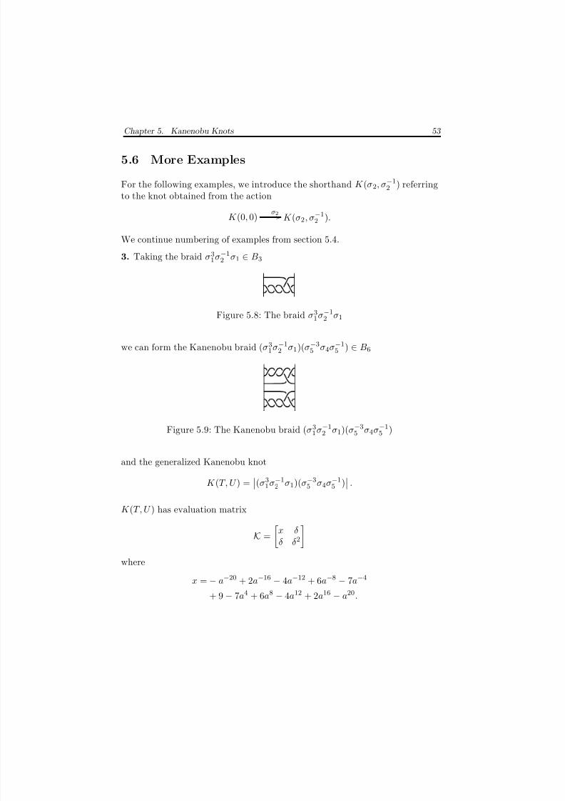
5.1 The Kanenobu knot K (T, U ) . . . . . . . . . . . . . . . . . . . . . . . . . . . . . . . . . . . . . 375.2 Distinct knots that are not Conway mutants . . . . . . . . . . . . . . . . . . . . . . 435.3 Example 1 . . . . . . . . . . . . . . . . . . . . . . . . . . . . . . . . . . . . . . . . . . . . . . . . . . . . . . . . 475.4 Example 2 . . . . . . . . . . . . . . . . . . . . . . . . . . . . . . . . . . . . . . . . . . . . . . . . . . . . . . . . 495.5 Another diagram of the Kanenobu knot K (T, U ) . . . . . . . . . . . . . . . . . . 505.6 The link |β | . . . . . . . . . . . . . . . . . . . . . . . . . . . . . . . . . . . . . . . . . . . . . . . . . . . . . . 505.7 The closure of a Kanenobu braid . . . . . . . . . . . . . . . . . . . . . . . . . . . . . . . . . . 515.8 The braid σ3
1σ−12 σ1 . . . . . . . . . . . . . . . . . . . . . . . . . . . . . . . . . . . . . . . . . . . . . . . 535.9 The Kanenobu braid (σ3
1
σ−1
2
σ1)(σ−3
5
σ4σ−1
5
) . . . . . . . . . . . . . . . . . . . . . . . 535.10 The knot (σ3
1σ−12 σ1)(σ−35 σ4σ−15 ) . . . . . . . . . . . . . . . . . . . . . . . . . . . . . . . . . 545.11 The knot K (0, 0) ∼ 52 # 5 2 . . . . . . . . . . . . . . . . . . . . . . . . . . . . . . . . . . . . . . . 555.12 The knot K (σ2, σ−12 ) . . . . . . . . . . . . . . . . . . . . . . . . . . . . . . . . . . . . . . . . . . . . . . 555.13 The braid σ2
1σ−32 σ1 . . . . . . . . . . . . . . . . . . . . . . . . . . . . . . . . . . . . . . . . . . . . . . . 565.14 The Kanenobu braid (σ2
1σ−32 σ1)(σ−25 σ34σ−15 ) . . . . . . . . . . . . . . . . . . . . . . . 56
5.15 The knot(σ2
1σ−32 σ1)(σ−25 σ34σ−15 )
. . . . . . . . . . . . . . . . . . . . . . . . . . . . . . . . . 575.16 The knot K (0, 0) ∼ 61 # 6 1 . . . . . . . . . . . . . . . . . . . . . . . . . . . . . . . . . . . . . . . 585.17 The knot K (σ2, σ−12 ) . . . . . . . . . . . . . . . . . . . . . . . . . . . . . . . . . . . . . . . . . . . . . . 585.18 The 2-bridge link obtained from β ∈ B3. . . . . . . . . . . . . . . . . . . . . . . . . . . 595.19 The square knot 31 # 31 . . . . . . . . . . . . . . . . . . . . . . . . . . . . . . . . . . . . . . . . . . 605.20 The knot (σ1σ−12 σ1)(σ−15 σ4σ−15 ). . . . . . . . . . . . . . . . . . . . . . . . . . . . . . . . . . 60
6.1 The Thislethwaite link H (T, U ) . . . . . . . . . . . . . . . . . . . . . . . . . . . . . . . . . . . 636.2 The link H (0, 0) . . . . . . . . . . . . . . . . . . . . . . . . . . . . . . . . . . . . . . . . . . . . . . . . . . 636.3 The braid ω ∈ B3 . . . . . . . . . . . . . . . . . . . . . . . . . . . . . . . . . . . . . . . . . . . . . . . . . 666.4 The link H (T ω, U ω
−1
) . . . . . . . . . . . . . . . . . . . . . . . . . . . . . . . . . . . . . . . . . . . . 676.5 The result of ω2 acting on H (T, U ) . . . . . . . . . . . . . . . . . . . . . . . . . . . . . . . . 686.6 The result of ω4 acting on H (T, U ) . . . . . . . . . . . . . . . . . . . . . . . . . . . . . . . . 68
v
8/3/2019 Liam Thomas Watson- Knots, Tangles and Braid Actions
http://slidepdf.com/reader/full/liam-thomas-watson-knots-tangles-and-braid-actions 7/82
List of Figures vi
6.7 A non-trivial, 2-component link . . . . . . . . . . . . . . . . . . . . . . . . . . . . . . . . . . . 696.8 A non-trivial, 2-component link . . . . . . . . . . . . . . . . . . . . . . . . . . . . . . . . . . . 706.9 A non-trivial, 3-component link . . . . . . . . . . . . . . . . . . . . . . . . . . . . . . . . . . . 71
vi

8/3/2019 Liam Thomas Watson- Knots, Tangles and Braid Actions
http://slidepdf.com/reader/full/liam-thomas-watson-knots-tangles-and-braid-actions 8/82
Acknowledgement
It’s a strange process, writing down the details to something you’ve been work-ing on for some time. And while it is a particularly solitary experience, thefinal product is not accomplished on you’re own. To this end, there are manypeople that should be recognised as part of this thesis.
First, I would like to thank my supervisor Dale Rolfsen for ongoing patience,guidance and instruction. It has been a privilege and a pleasure to learn fromDale throughout my undergraduate and masters degrees, and I am grateful forhis generous support, both intellectual and financial. I have learned so much.
Of course, I am indebted to all of my teachers as this work comprises much of what I have learned so far. However, I would like to single out Bill Casselman,as the figures required for this thesis could not have been produced withouthis guidance.
To my parents, Peter and Katherine Watson, family and friends, I am sofortunate to have a support network that allows me to pursue mathematics.In particular, I would like to thank Erin Despard for continued encouragement,support and perspective, everyday.
vii
8/3/2019 Liam Thomas Watson- Knots, Tangles and Braid Actions
http://slidepdf.com/reader/full/liam-thomas-watson-knots-tangles-and-braid-actions 9/82
Chapter 1
Introduction
The study of knots begins with a straight-forward question: Can we distinguishbetween two closed loops, embedded in three dimensions? This leads naturallyto a more general question of links, that is, the ability to distinguish betweentwo systems of embedded closed loops. Early work by Alexander [1, 2], Artin [3,4], Markov [24] and Reidemeister [29] made inroads into the subject, developingthe first knot and link invariants, as well as the combinatorial and algebraiclanguages with which to approach the subject. The subtle relationship betweenthe combinatorial and algebraic descriptions continue to set the stage for the
study of knots and links.
With the discovery of the Jones polynomial [15] in 1985, along with a twovariable generalization [12] shortly thereafter, the study of knots was givennew focus. These new polynomial invariants could be viewed as combinatorialobjects, derived directly from a diagram of the knot, or as algebraic objects,resulting from representations of the braid group. However, although the newpolynomials were able to distinguish between knots that had previously causeddifficulties, they led to new questions in the study of knots that have yet to beanswered.
In particular, we are led to the phenomenon of distinct knots having the same
Jones polynomial. There are many examples of families of knots that sharecommon Jones polynomials. Such examples have given way to a range of toolsto describe this occurrence [30, 31]. In particular, it is unknown if there is anon-trivial knot that has trivial Jones polynomial. This question motivates theunderstanding of knots that cannot be distinguished by the Jones polynomial,as well as the development of examples of such along with tools to explainthe phenomenon. The prototypical method for producing two knots having
1
8/3/2019 Liam Thomas Watson- Knots, Tangles and Braid Actions
http://slidepdf.com/reader/full/liam-thomas-watson-knots-tangles-and-braid-actions 10/82
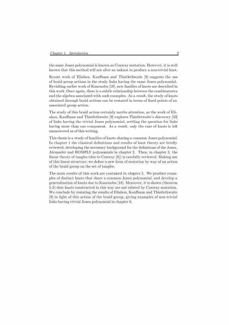
Chapter 1. Introduction 2
the same Jones polynomial is known as Conway mutation. However, it is wellknown that this method will not alter an unknot to produce a non-trivial knot.
Recent work of Eliahou, Kauffman and Thistlethwaite [9] suggests the useof braid group actions in the study links having the same Jones polynomial.Revisiting earlier work of Kanenobu [18], new families of knots are described inthis work. Once again, there is a subtle relationship between the combinatoricsand the algebra associated with such examples. As a result, the study of knotsobtained through braid actions can be restated in terms of fixed points of an
associated group action.The study of this braid action certainly merits attention, as the work of Eli-ahou, Kauffman and Thistlethwaite [9] explores Thistletwaite’s discovery [33]of links having the trivial Jones polynomial, settling the question for linkshaving more than one component. As a result, only the case of knots is leftunanswered as of this writing.
This thesis is a study of families of knots sharing a common Jones polynomial.In chapter 1 the classical definitions and results of knot theory are brieflyreviewed, developing the necessary background for the definitions of the Jones,Alexander and HOMFLY polynomials in chapter 2. Then, in chapter 3, thelinear theory of tangles (due to Conway [8]) is carefully reviewed. Making useof this linear structure, we define a new form of mutation by way of an actionof the braid group on the set of tangles.
The main results of this work are contained in chapter 5. We produce exam-ples of distinct knots that share a common Jones polynomial, and develop ageneralization of knots due to Kanenobu [18]. Moreover, it is shown (theorem5.3) that knots constructed in this way are not related by Conway mutation.We conclude by restating the results of Eliahou, Kauffman and Thistlethwaite[9] in light of this action of the braid group, giving examples of non-triviallinks having trivial Jones polynomial in chapter 6.
8/3/2019 Liam Thomas Watson- Knots, Tangles and Braid Actions
http://slidepdf.com/reader/full/liam-thomas-watson-knots-tangles-and-braid-actions 11/82
Chapter 2
Knots, Links and Braids
2.1 Knots and Links
A knot K is a smooth or piecewise linear embedding of a closed curve in a3-dimensional manifold. Usually, the manifold of choice is either R
3 or S3, so
that the knot K may be denoted
S1 → R
3 ⊂ S3.
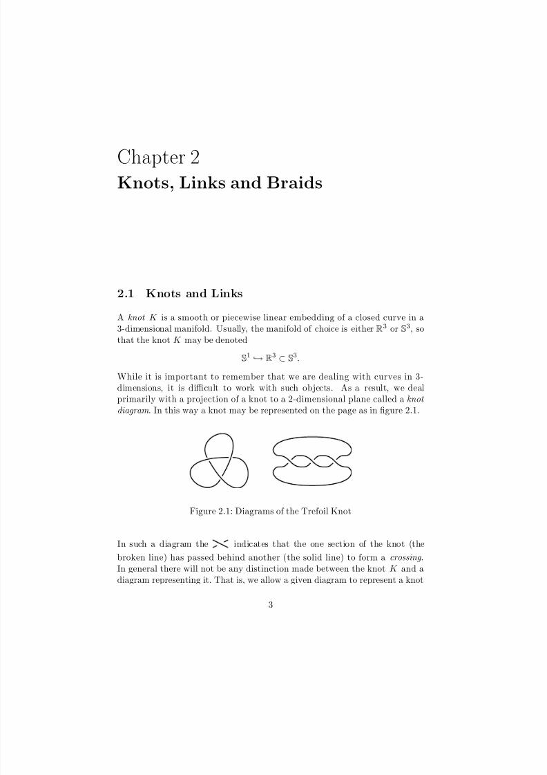
While it is important to remember that we are dealing with curves in 3-dimensions, it is difficult to work with such objects. As a result, we dealprimarily with a projection of a knot to a 2-dimensional plane called a knot diagram . In this way a knot may be represented on the page as in figure 2.1.
Figure 2.1: Diagrams of the Trefoil Knot
In such a diagram the indicates that the one section of the knot (the
broken line) has passed behind another (the solid line) to form a crossing .In general there will not be any distinction made between the knot K and adiagram representing it. That is, we allow a given diagram to represent a knot
3
8/3/2019 Liam Thomas Watson- Knots, Tangles and Braid Actions
http://slidepdf.com/reader/full/liam-thomas-watson-knots-tangles-and-braid-actions 12/82
Chapter 2. Knots, Links and Braids 4
and denote the diagram by K also. It should be pointed out, however, thatthere are many diagrams for any given knot. Indeed, K and K are equivalent knots (denoted K ∼ K ) if they are related by isotopy in S
3. Therefore, thediagrams for K and K may be very different.
An n-component link is a collection of knots. That is, a link is a disjoint unionof embedded circles
n
i=1
S1i → R
3 ⊂ S3
where eachS1i → R
3 ⊂ S3
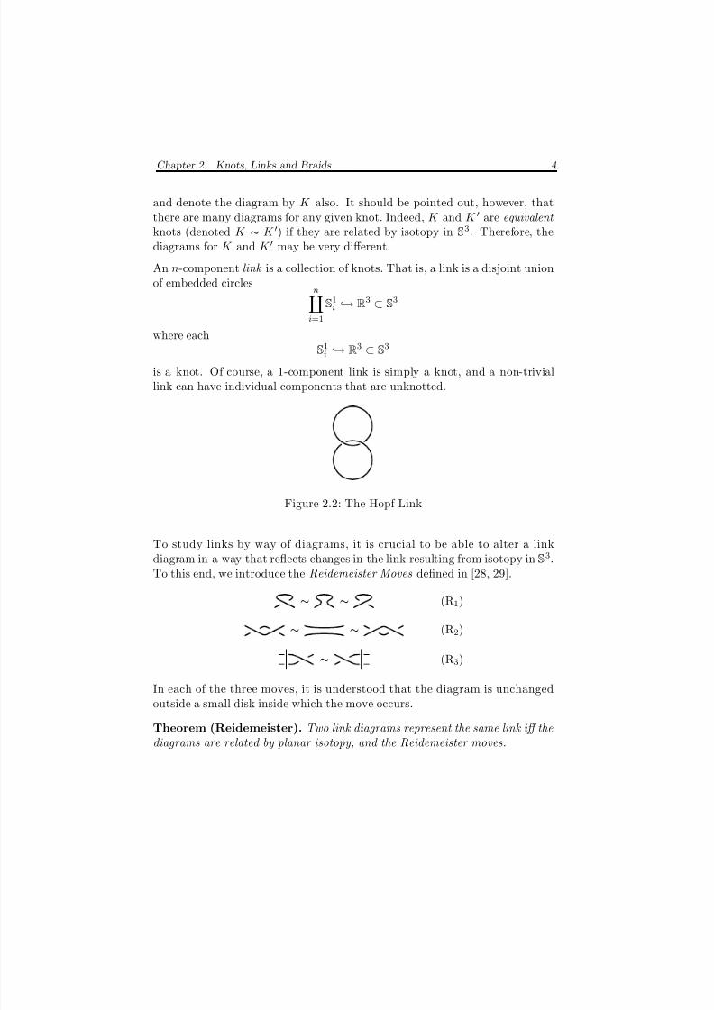
is a knot. Of course, a 1-component link is simply a knot, and a non-triviallink can have individual components that are unknotted.
Figure 2.2: The Hopf Link
To study links by way of diagrams, it is crucial to be able to alter a linkdiagram in a way that reflects changes in the link resulting from isotopy in S
3.To this end, we introduce the Reidemeister Moves defined in [28, 29].
∼ ∼ (R1)
∼ ∼ (R2)
∼ (R3)
In each of the three moves, it is understood that the diagram is unchangedoutside a small disk inside which the move occurs.
Theorem (Reidemeister). Two link diagrams represent the same link iff thediagrams are related by planar isotopy, and the Reidemeister moves.
8/3/2019 Liam Thomas Watson- Knots, Tangles and Braid Actions
http://slidepdf.com/reader/full/liam-thomas-watson-knots-tangles-and-braid-actions 13/82
Chapter 2. Knots, Links and Braids 5
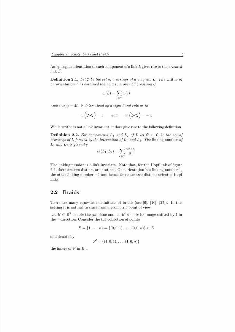
Assigning an orientation to each component of a link L gives rise to the oriented link L.
Definition 2.1. Let C be the set of crossings of a diagram L. The writhe of an orientation L is obtained taking a sum over all crossings C
w( L) =c∈C
w(c)
where w(c) =
±1 is determined by a right hand rule as in
w
= 1 and w
= −1.
While writhe is not a link invariant, it does give rise to the following definition.
Definition 2.2. For components L1 and L2 of L let C ⊂ C be the set of crossings of L formed by the interaction of L1 and L2. The linking number of L1 and L2 is given by
lk(L1, L2) =c∈C
w(c)
2.
The linking number is a link invariant. Note that, for the Hopf link of figure2.2, there are two distinct orientations. One orientation has linking number 1,the other linking number −1 and hence there are two distinct oriented Hopf links.
2.2 Braids
There are many equivalent definitions of braids (see [6], [10], [27]). In thissetting it is natural to start from a geometric point of view.
Let E
⊂R3 denote the yz-plane and let E denote its image shifted by 1 in
the x direction. Consider the the collection of points
P = {1, . . . , n} = {(0, 0, 1), . . . , (0, 0, n)} ⊂ E
and denote byP = {(1, 0, 1), . . . , (1, 0, n)}
the image of P in E .
8/3/2019 Liam Thomas Watson- Knots, Tangles and Braid Actions
http://slidepdf.com/reader/full/liam-thomas-watson-knots-tangles-and-braid-actions 14/82
Chapter 2. Knots, Links and Braids 6
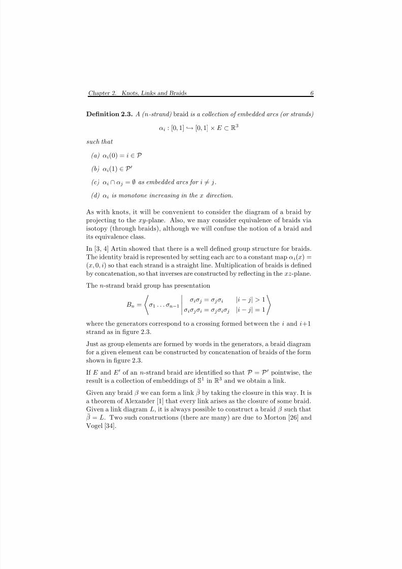
Definition 2.3. A ( n-strand) braid is a collection of embedded arcs (or strands)
αi : [0, 1] → [0, 1] × E ⊂ R3
such that
(a) αi(0) = i ∈ P (b) αi(1) ∈ P
(c) αi ∩
α j
=∅
as embedded arcs for i= j.
(d) αi is monotone increasing in the x direction.
As with knots, it will be convenient to consider the diagram of a braid byprojecting to the xy-plane. Also, we may consider equivalence of braids viaisotopy (through braids), although we will confuse the notion of a braid andits equivalence class.
In [3, 4] Artin showed that there is a well defined group structure for braids.The identity braid is represented by setting each arc to a constant map αi(x) =(x, 0, i) so that each strand is a straight line. Multiplication of braids is definedby concatenation, so that inverses are constructed by reflecting in the xz-plane.
The n-strand braid group has presentation
Bn =
σ1 . . . σn−1
σiσ j = σ jσi |i − j| > 1
σiσ jσi = σ jσiσ j |i − j| = 1
where the generators correspond to a crossing formed between the i and i+1strand as in figure 2.3.
Just as group elements are formed by words in the generators, a braid diagramfor a given element can be constructed by concatenation of braids of the formshown in figure 2.3.
If E and E
of an n-strand braid are identified so that P = P pointwise, theresult is a collection of embeddings of S
1 in R3 and we obtain a link.
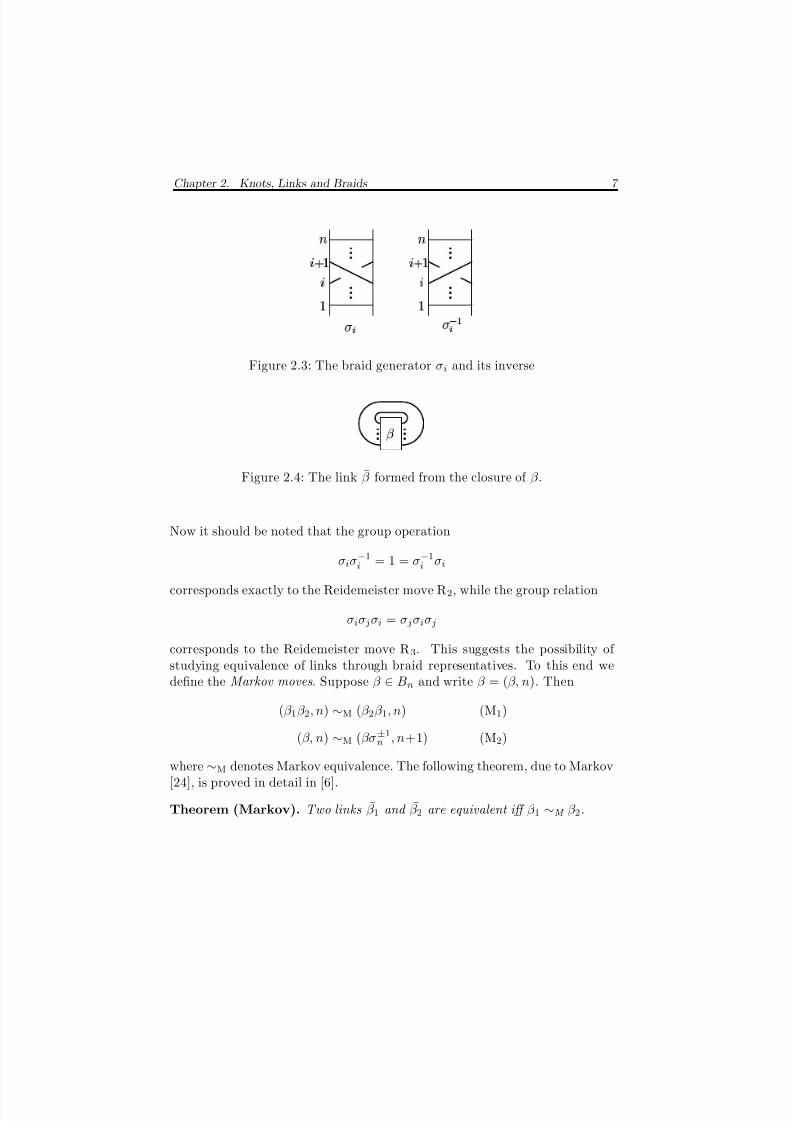
Given any braid β we can form a link β by taking the closure in this way. It isa theorem of Alexander [1] that every link arises as the closure of some braid.Given a link diagram L, it is always possible to construct a braid β such thatβ = L. Two such constructions (there are many) are due to Morton [26] andVogel [34].
8/3/2019 Liam Thomas Watson- Knots, Tangles and Braid Actions
http://slidepdf.com/reader/full/liam-thomas-watson-knots-tangles-and-braid-actions 15/82
Chapter 2. Knots, Links and Braids 7
¡
¡
¡
¢
£
¤ ¥ §
©
! " $
&
Figure 2.3: The braid generator σi and its inverse
'
(
(
( )
)
)
Figure 2.4: The link β formed from the closure of β .
Now it should be noted that the group operation
σiσ−1i = 1 = σ−1i σi
corresponds exactly to the Reidemeister move R2, while the group relation
σiσ jσi = σ jσiσ j
corresponds to the Reidemeister move R3. This suggests the possibility of studying equivalence of links through braid representatives. To this end wedefine the Markov moves. Suppose β ∈ Bn and write β = (β, n). Then
(β 1β 2, n) ∼M (β 2β 1, n) (M1)
(β, n) ∼M (βσ±1n , n+1) (M2)
where ∼M denotes Markov equivalence. The following theorem, due to Markov[24], is proved in detail in [6].
Theorem (Markov). Two links β 1 and β 2 are equivalent iff β 1 ∼M β 2.
8/3/2019 Liam Thomas Watson- Knots, Tangles and Braid Actions
http://slidepdf.com/reader/full/liam-thomas-watson-knots-tangles-and-braid-actions 16/82
Chapter 3
Polynomials
3.1 The Jones Polynomial
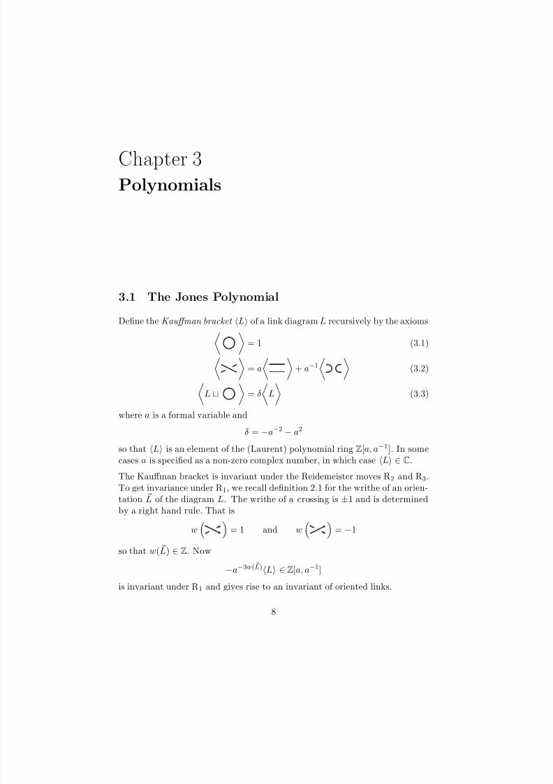
Define the Kauffman bracket L of a link diagram L recursively by the axioms = 1 (3.1)
= a
+ a−1
(3.2)
L
= δ
L
(3.3)
where a is a formal variable and
δ = −a−2 − a2
so that L is an element of the (Laurent) polynomial ring Z[a, a−1]. In somecases a is specified as a non-zero complex number, in which case L ∈ C.
The Kauffman bracket is invariant under the Reidemeister moves R2 and R3.To get invariance under R1, we recall definition 2.1 for the writhe of an orien-tation L of the diagram L. The writhe of a crossing is ±1 and is determined
by a right hand rule. That is
w
= 1 and w
= −1
so that w( L) ∈ Z. Now
−a−3w( L)L ∈ Z[a, a−1]
is invariant under R1 and gives rise to an invariant of oriented links.
8
8/3/2019 Liam Thomas Watson- Knots, Tangles and Braid Actions
http://slidepdf.com/reader/full/liam-thomas-watson-knots-tangles-and-braid-actions 17/82
Chapter 3. Polynomials 9
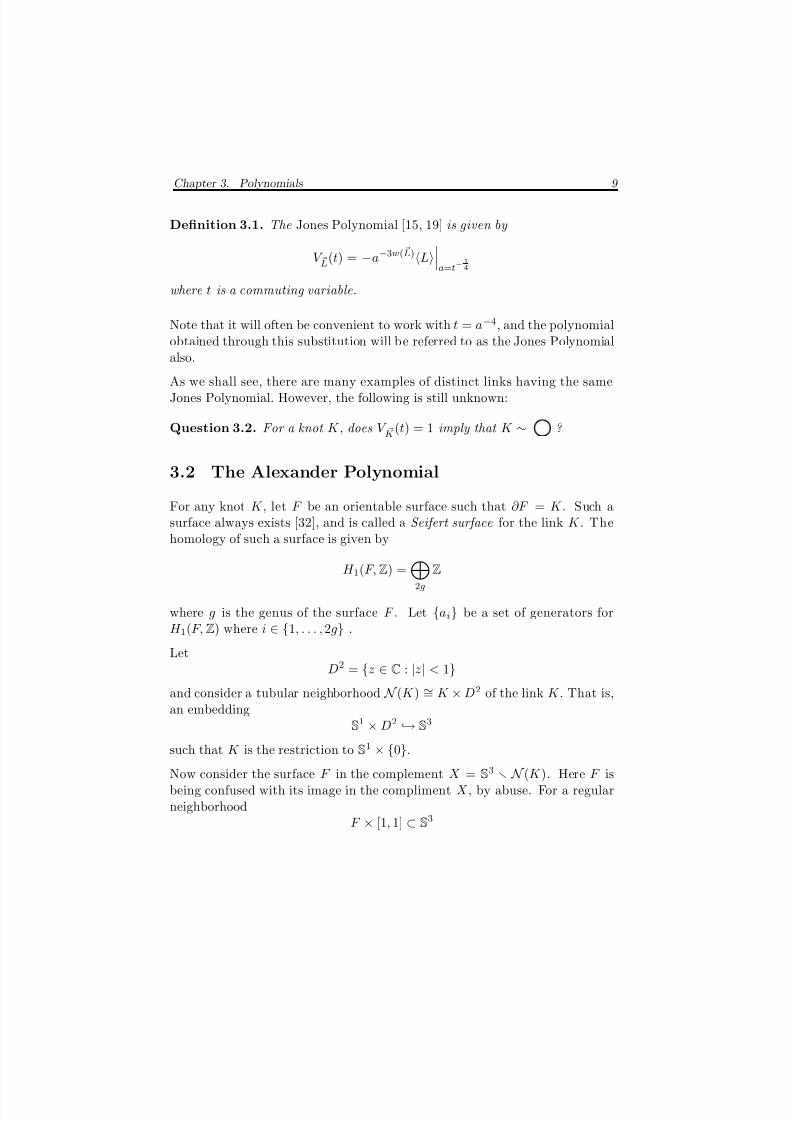
Definition 3.1. The Jones Polynomial [15, 19] is given by
V L(t) = −a−3w( L)L
a=t−
14
where t is a commuting variable.
Note that it will often be convenient to work with t = a−4, and the polynomialobtained through this substitution will be referred to as the Jones Polynomialalso.
As we shall see, there are many examples of distinct links having the sameJones Polynomial. However, the following is still unknown:
Question 3.2. For a knot K , does V K (t) = 1 imply that K ∼ ?
3.2 The Alexander Polynomial
For any knot K , let F be an orientable surface such that ∂F = K . Such asurface always exists [32], and is called a Seifert surface for the link K . Thehomology of such a surface is given by
H 1(F, Z) =2g
Z
where g is the genus of the surface F . Let {ai} be a set of generators forH 1(F, Z) where i ∈ {1, . . . , 2g} .
LetD2 = {z ∈ C : |z| < 1}
and consider a tubular neighborhood N (K ) ∼= K × D2 of the link K . That is,an embedding
S1
×D2
→S3
such that K is the restriction to S1 × {0}.
Now consider the surface F in the complement X = S3
N (K ). Here F isbeing confused with its image in the compliment X , by abuse. For a regularneighborhood
F × [1, 1] ⊂ S3
8/3/2019 Liam Thomas Watson- Knots, Tangles and Braid Actions
http://slidepdf.com/reader/full/liam-thomas-watson-knots-tangles-and-braid-actions 18/82
Chapter 3. Polynomials 10
there are natural inclusions
i± : F → F × {±1}where F = F ×{0} is the Seifert surface in X . Therefore a cycle x ∈ H 1(F, Z)gives rise to a cycle x± = i± (x) ∈ H 1(X, Z).
Definition 3.3. The Seifert Form is the bilinear form
v : H 1(F, Z) × H 1(F, Z) → Z
(x, y
) →lk
(x, y+
)and it is represented by the Seifert Matrix
V =
lk(ai, a+ j )
where y+ = i+ (y).
The aim is to construct X , the infinite cyclic cover [25, 32] of the knot com-plement X = S
3 N (K ). To do this, start with a countable collection {X i}i∈Z
of X i = X (F × (−, ))
for some small ∈ (0, 1). The boundary of this space contains two identicalcopies of F denoted byF ± = F × {±},
and the infinite cyclic cover of X is defined
X =
i∈Z X i
F +i ∼ F −i+1
by identifying F +i ⊂ ∂X i with F −i+1 ⊂ ∂X i+1 for each i ∈ Z.
The space obtained corresponds to the short exact sequence
1 / / π1 X / / π1X / / H 1(X, Z) / / 0
α / / lk
α, K
so that the infinite cyclic group H 1(X, Z) = t gives the covering translationsof X X . Now H 1(X, Z), although typically not finitely generated as anabelian group, is finitely generated as a Z[t, t−1]-module by the {ai}. Thevariable t corresponds to the t-action taking X i to X i+1.
8/3/2019 Liam Thomas Watson- Knots, Tangles and Braid Actions
http://slidepdf.com/reader/full/liam-thomas-watson-knots-tangles-and-braid-actions 19/82
Chapter 3. Polynomials 11
Definition 3.4. H 1(X, Z) is called the Alexander module and has modulepresentation V − tV , where V is the Seifert matrix. This is a knot invariant.
This gives rise to another polynomial invariant due to Alexander [2].
Definition 3.5. The Laurent polynomial
∆K (t).
= det(V − tV ) ∈ Z[t, t−1]
is an invariant of the knot K called the Alexander polynomial. It is defined up to multiplication by a unit ±t±n (indicated by .=).
This knot invariant is of particular interest due to this topological construction.
Question 3.6. Is there a similar topological interpretation for the Jones poly-nomial?
On the other hand, it is easy to generate knots K such that ∆K (t) = 1 (seefor example, [32]).
Theorem 3.7. For any knot K , ∆K (t).
= ∆K (t−1).
proof. Given the n × n Seifert matrix V,
∆K .
= det(V − tV )
= det(V − tV )
= (−t)n det(V − t−1V ).
= ∆K (t−1).
Theorem 3.8. For any knot K , ∆K (1) =
±1.
proof. Setting t = 1 and using the standard (symplectic) basis for H 1(F, Z)
8/3/2019 Liam Thomas Watson- Knots, Tangles and Braid Actions
http://slidepdf.com/reader/full/liam-thomas-watson-knots-tangles-and-braid-actions 20/82
Chapter 3. Polynomials 12
gives
V − V =
lk(ai, a+ j ) − lk(a j , a+i )
=
lk(ai, a+ j ) − lk(a− j , ai)
=
lk(ai, a+ j ) − lk(ai, a− j )
=
0 1
−1 0
0 1−1 0. . .
0 1−1 0
therefore
∆K (1) = ± det(V − V ) = ±1.
Corollary 3.9. For any knot K
∆K (t) .= c0 + c1(t−1 + t1) + c2(t−1 + t1)2 + · · ·where ci ∈ Z.
proof. The symmetry given by ∆K (t).
= ∆K (t−1) gives rise to the form
∆K (t).
=mk=0
bktk
where cm−r = ±cr, and the same choice of sign is made for each r. Now m
must be even, since m odd gives rise to ∆K (1) even, contradicting theorem3.8. Further, if cm−r = −cr then cm/2 = 0 and
∆K (1) =mk=0
bk = 0,
again contradicting theorem 3.8. Therefore cm−r = cr, and
∆K (t).
= c0 + c1(t−1 + t1) + c2(t−1 + t1)2 + · · ·as required.
8/3/2019 Liam Thomas Watson- Knots, Tangles and Braid Actions
http://slidepdf.com/reader/full/liam-thomas-watson-knots-tangles-and-braid-actions 21/82
Chapter 3. Polynomials 13
We will see the form given in corollary 3.9 in the next section. Together withthe normalization ∆K (1) = 1, it is sometimes referred to as the Alexander-Conway polynomial as it has a recursive definition, originally noticed by Alexan-der [2] and later exploited by Conway [8].
It should be noted that there are generalizations of this construction to invari-ants of oriented links that have been omitted. Nevertheless, we shall see thatthe recursive definition of ∆K (t) is defined for all oriented links.
3.3 The HOMFLY Polynomial
A two variable polynomial [12, 16] that restricts to each of the polynomialsintroduced may be defined, albeit by very different means.
The n-strand braid group Bn generates a group algebra H n over Z[q, q−1] whichhas relations
(i) σiσ j = σ jσi for |i − j| > 1
(ii) σiσ jσi = σ jσiσ j for |i − j| = 1
(iii) σ2i = (q − 1)σi + q ∀ i ∈ {1, . . . , n−1}
called the Hecke algebra. By allowing q to take values in C, H n can be seenas a quotient of the group algebra CBn. Just as
{1} < B2 < B3 < B4 < · · ·we have that
Z[q, q−1] ⊂ H 2 ⊂ H 3 ⊂ H 4 ⊂ ·· · .
Note that for q = 1, the relation (iii) reduces to σ2i = 1 and we obtain the
relations for the symmetric group S n.
Definition 3.10. Sets of positive permutation braids may be defined recur-sively via
Σ0 = {1}Σi = {1} ∪ σiΣi−1 for i > 0.
A monomial m ∈ H n is called normal if it has the form
m = m1m2 . . . mn−1
where mi ∈ Σi.
8/3/2019 Liam Thomas Watson- Knots, Tangles and Braid Actions
http://slidepdf.com/reader/full/liam-thomas-watson-knots-tangles-and-braid-actions 22/82
Chapter 3. Polynomials 14
The normal monomials form a basis for H n, and it follows that
dimZ[q,q−1](H n) = n!.
Moreover, this basis allows us to present any element of H n+1 in the form
x1 + x2σnx3
for xi ∈ H n. The relation (i) implies that
xσn = σnx
whenever x ∈ H n−1, giving rise to the decomposition
H n+1∼= H n ⊕ H n ⊗H n−1 H n
.
Now we define a linear trace function
tr : H n −→ Z[q±1, z]
σi −→ z
that is normalized so that tr(1) = 1.
Theorem 3.11. tr(x1x2) = tr(x2x1) for xi∈
H n.
proof. By linearity, it suffices to show that tr(m1m2) = tr(m2m1) for nor-mal monomials mi ∈ H n. Since the theorem is clearly true for the normalmonomials of H 2, we proceed by induction.
Suppose first that m1 = m1σnm
1 where m1, m
1 ∈ H n and m2 ∈ H n (that is,m2 contains no σn). Then
tr(m1m2) = tr(m1σnm
1m2)
= z tr(m1m
1m2)
= z tr(m2m1m
1) by induction
= tr(m2m
1σnm
1)= tr(m2m1).
Now more generally write
m1 = m1σnm
1 and m2 = m2σnm
2
where mi, m
i ∈ H n. In this case we will make use of the following:
8/3/2019 Liam Thomas Watson- Knots, Tangles and Braid Actions
http://slidepdf.com/reader/full/liam-thomas-watson-knots-tangles-and-braid-actions 23/82
Chapter 3. Polynomials 15
(1) tr(µ1σnµ2σn) = tr(σnµ1σnµ2)
(2) tr(µ1σnµ2σnµ3) = tr(µ3µ1σnµ2σn)
where µi ∈ H n are in normal form so that µi = µiσn−1µi with µi, µi ∈ H n−1.
(1)
tr(µ1σnµ2σn) = tr(µ1σnµ2σn−1µ2σn)
= tr(µ1µ2σnσn−1σnµ2) using (i)
= tr(µ1µ
2σn−1σnσn−1µ
2) using (ii)= z tr(µ1µ2σ2
n−1µ2)
= z tr(µ1µ2[(q − 1)σn−1 + q]µ2) using (iii)
= z(q − 1)tr(µ1µ2σn−1µ2) + zq tr(µ1µ2µ2)
= z(q − 1)tr(µ1µ2) + zq tr(µ1σn−1µ1µ2µ2)
= z(q − 1)tr(µ1µ2) + zq tr(µ1µ1µ2σn−1µ2) induction
= z(q − 1)tr(µ1µ2) + zq tr(µ1µ1µ2)
= z tr(µi[(q − 1)σn−1 + q]µ1µ2)
= z tr(µ1σ2n−1µ1µ2) using (iii)
= tr(µ
1σn−1σnσn−1µ
1µ2)
= tr(µ1σnσn−1σnµ1µ2) using (ii)
= tr(σnµ1σn−1µ1σnµ2) using (i)
= tr(σnµ1σnµ2)
(2)
tr(µ1σnµ2σnµ3)
= tr(µ1µ2σnµ3σn) applying (1)
= tr(µ1µ2σnµ3σn−1µ3σn)
= z tr(µ1µ2µ3σ2n−1µ3) as above
= z(q − 1)tr(µ1µ2µ3σn−1µ
3) + zq tr(µ1µ2µ
3µ3) using (iii)
= z(q − 1)tr(µ3σn−1µ3µ1µ2) + zq tr(µ3µ3µ1µ2) induction
= z tr(µ3σ2n−1µ3µ1µ2) using (iii)
= tr(σnµ3σn−1µ3σnµ1µ2) as above
= tr(σnµ3σnµ1µ2)
= tr(µ3µ1σnµ2σn) applying (1)
8/3/2019 Liam Thomas Watson- Knots, Tangles and Braid Actions
http://slidepdf.com/reader/full/liam-thomas-watson-knots-tangles-and-braid-actions 24/82
Chapter 3. Polynomials 16
Now the proof is complete, since
tr(m1m2) = tr(m1σnm
1m2σnm
2)
= tr(m2m
1σnm1m
2σn) by (2)
= tr(σnm2m
1σnm1m
2) by (1)
= tr(m2σnm
2m1σnm
1) by (2)
= tr(m2m1).
Now since elements of H n+1 are of the form x1 + x2σnx3 where xi ∈ H n, thetrace function may be extended from H n to H n+1 by
tr(x1 + x2σnx3) = tr(x1) + z tr(x2x3).
The aim is to use the trace function to define a link invariant. In particularwe would like to make use of this trace on braids in the composite
Bn −→ H n −→ Z[q±1, z].
To do this, we introduce a change of variables λ = w
qz
where
z = − 1 − q
1 − λqand w = −λq(1 − q)
1 − λq
so that
λ =1 − q + z
zq.
Definition 3.12. The HOMFLY polynomial is given by
X β (q, λ) =
− 1 − λq√
λ(1 − q)
n−1 √λe
tr(β )
where β ∈ Bn is a monomial in H n and e = e(β ) is the exponent sum of β (equivalently, the abelianization Bn → Z).
Note that the closure of the identity braid in Bn gives the n component unlink
· · · n
8/3/2019 Liam Thomas Watson- Knots, Tangles and Braid Actions
http://slidepdf.com/reader/full/liam-thomas-watson-knots-tangles-and-braid-actions 25/82
Chapter 3. Polynomials 17
and the HOMFLY polynomial for this link is given by− 1 − λq√
λ(1 − q)
n−1. (3.4)
Theorem 3.13. Let β = L then X L(q, λ) ∈ Z
q±1,
√λ±1
is a link invari-
ant.
proof. By Markov’s theorem, we need only check that X L(q, λ) is invariantunder M1 and M2. The fact that tr(β 1β 2) = tr(β 2β 1) from Theorem 3.11 givesinvariance under M1, so it remains to check invariance under M2. Supposethen that β ∈ Bn. With the above substitution we have
tr(σn) = − 1 − q
1 − λq
so that
X βσn(q, λ) =
− 1 − λq√
λ(1 − q)
n √λe+1
tr(βσi)
= √λ− 1 − λq√λ(1 − q)
− 1 − q1 − λq
X β (q, λ)
= X β (q, λ).
Further, from (iii) we can derive
σ2i = (q − 1)σi + q
σi = (q − 1) + qσ−1i
qσ−1i = σi + 1 − q
σ−1i = q−1σi + q−1 − 1
8/3/2019 Liam Thomas Watson- Knots, Tangles and Braid Actions
http://slidepdf.com/reader/full/liam-thomas-watson-knots-tangles-and-braid-actions 26/82
Chapter 3. Polynomials 18
hence
tr(σ−1i ) = tr(q−1σi + q−1 − 1)
= q−1 tr(σi) + q−1 − 1
= q−1
− 1 − q
1 − λq
+ q−1 − 1
= q−1
− 1 − q
1 − λq+ 1
− 1
= q−1−1 + q + 1 − λq1 − λq
− 1
=1 − λ − 1 + λq
1 − λq
= −λ1 − q
1 − λq.
Thus
X βσ−1n
(q, λ) =
− 1 − λq√
λ(1 − q)
n √λe−1
tr(βσ−11 )
= 1√λ− 1 −
λq√
λ(1 − q)−λ 1 −
q
1 − λqX β (q, λ)
= X β (q, λ)
and X β (q, λ) is a link invariant.
Both the single variable polynomials may be retrieved from the HOMFLYpolynomial via the substitutions
V L(t) = X L(t, t)
∆L(t).
= X L t, t−1
.
Another definition of the HOMFLY polynomial is possible. For β ∈ Bn supposethat L = β , oriented so that the generator σi is a positive crossing (that is,w(σi) = 1). Suppose that β contains some σi
1 and write
β = γ 1σiγ 2
1a similar construction is possible for σ−1i
8/3/2019 Liam Thomas Watson- Knots, Tangles and Braid Actions
http://slidepdf.com/reader/full/liam-thomas-watson-knots-tangles-and-braid-actions 27/82
8/3/2019 Liam Thomas Watson- Knots, Tangles and Braid Actions
http://slidepdf.com/reader/full/liam-thomas-watson-knots-tangles-and-braid-actions 28/82
Chapter 3. Polynomials 20
we can defineP L(t, x) = X L(q, λ)
where P L(t, x) ∈ Z[t±1, x±1] is computed recursively from the axioms
P (t, x) = 1 (3.5)
t−1P L+(t, x) − tP L−(t, x) = xP L0(t, x). (3.6)
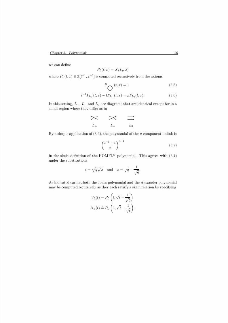
In this setting, L+, L− and L0 are diagrams that are identical except for in asmall region where they differ as in
L+ L− L0
By a simple application of (3.6), the polynomial of the n component unlink ist−1 − t
x
n−1(3.7)
in the skein definition of the HOMFLY polynomial. This agrees with (3.4)under the substitutions
t =
q
λ and x =√
q − 1√q
.
As indicated earlier, both the Jones polynomial and the Alexander polynomialmay be computed recursively as they each satisfy a skein relation by specifying
V L(t) = P L
t,
√t − 1√
t
∆L(t)
.= P L1,
√t
−1
√t .

8/3/2019 Liam Thomas Watson- Knots, Tangles and Braid Actions
http://slidepdf.com/reader/full/liam-thomas-watson-knots-tangles-and-braid-actions 29/82
Chapter 4
Tangles and Linear Maps
4.1 Conway Tangles
In the recursive computation of the Kauffman bracket of a link, the order inwhich the crossings are reduced is immaterial. In many cases it will be conve-nient to group crossings together in the course of computation. From Conway’spoint of view [8], such groupings or tangles form the building blocks of knotsand links. In addition, this point of view will allow us to take advantage of the well-developed tools of linear algebra.
Definition 4.1. Given a link L in S3 consider a 3-ball B3 ⊂ S
3 such that ∂B3 intersects L in exactly 4 points. The intersection B3 ∩ L is called a Conway tangle (or simply, a tangle) denoted by T . The exterior of the tangleS3 B3 ∩ L is called an external wiring, denoted by L T .
Note that, as S3 B3 is a ball, the external wiring L T is a tangle also.
Figure 4.1: Some diagrams of Conway tangles
A tangle, as a subset of a link, may be considered up to equivalence underisotopy. When a diagram of the link L is considered, a tangle may be repre-sented by a disk in the projection plane, with boundary intersecting the link
21
8/3/2019 Liam Thomas Watson- Knots, Tangles and Braid Actions
http://slidepdf.com/reader/full/liam-thomas-watson-knots-tangles-and-braid-actions 30/82
Chapter 4. Tangles and Linear Maps 22
in 4 points. Equivalence of tangle diagrams then, is given by the Reidemeistermoves, where the four boundary points are fixed.
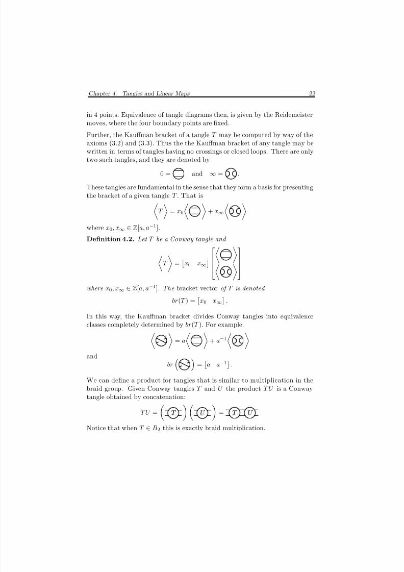
Further, the Kauffman bracket of a tangle T may be computed by way of theaxioms (3.2) and (3.3). Thus the the Kauffman bracket of any tangle may bewritten in terms of tangles having no crossings or closed loops. There are onlytwo such tangles, and they are denoted by
0 = and ∞ = .
These tangles are fundamental in the sense that they form a basis for presentingthe bracket of a given tangle T . That is
T
= x0
+ x∞
where x0, x∞ ∈ Z[a, a−1].
Definition 4.2. Let T be a Conway tangle and
T
=
x0 x∞
where x0, x∞ ∈ Z[a, a−1]. The bracket vector of T is denoted
br(T ) =
x0 x∞
.
In this way, the Kauffman bracket divides Conway tangles into equivalenceclasses completely determined by br(T ). For example,
= a
+ a−1
and
br
=
a a−1
.
We can define a product for tangles that is similar to multiplication in thebraid group. Given Conway tangles T and U the product T U is a Conwaytangle obtained by concatenation:
T U =
¡
= ¢ £
Notice that when T ∈ B2 this is exactly braid multiplication.
8/3/2019 Liam Thomas Watson- Knots, Tangles and Braid Actions
http://slidepdf.com/reader/full/liam-thomas-watson-knots-tangles-and-braid-actions 31/82
Chapter 4. Tangles and Linear Maps 23
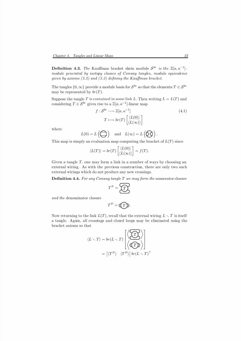
Definition 4.3. The Kauffman bracket skein module S br is the Z[a, a−1]-module generated by isotopy classes of Conway tangles, modulo equivalencegiven by axioms (3.2) and (3.3) defining the Kauffman bracket.
The tangles {0, ∞} provide a module basis for S br so that the elements T ∈ S brmay be represented by br(T ).
Suppose the tangle T is contained in some link L. Then writing L = L(T ) andconsidering T ∈ S br gives rise to a Z[a, a−1]-linear map
f : S br
−→ Z[a, a−1
] (4.1)
T −→ br(T )
L(0)L(∞)
where
L(0) = L
and L(∞) = L
.
This map is simply an evaluation map computing the bracket of L(T ) since
L(T ) = br(T )
L(0)L(∞)
= f (T ).
Given a tangle T , one may form a link in a number of ways by choosing an
external wiring. As with the previous construction, there are only two suchexternal wirings which do not produce any new crossings.
Definition 4.4. For any Conway tangle T we may form the numerator closure
T N =
and the denominator closure
T D = ¡ .
Now returning to the link L(T ), recall that the external wiring L T is itself a tangle. Again, all crossings and closed loops may be eliminated using thebracket axioms so that
L T = br(L T )
¢
£
=T N T D br(L T )
8/3/2019 Liam Thomas Watson- Knots, Tangles and Braid Actions
http://slidepdf.com/reader/full/liam-thomas-watson-knots-tangles-and-braid-actions 32/82
Chapter 4. Tangles and Linear Maps 24
This gives rise to another Z[a, a−1]-linear evaluation map
S br −→ Z[a, a−1] (4.2)
L T −→ T N T D br(L T )
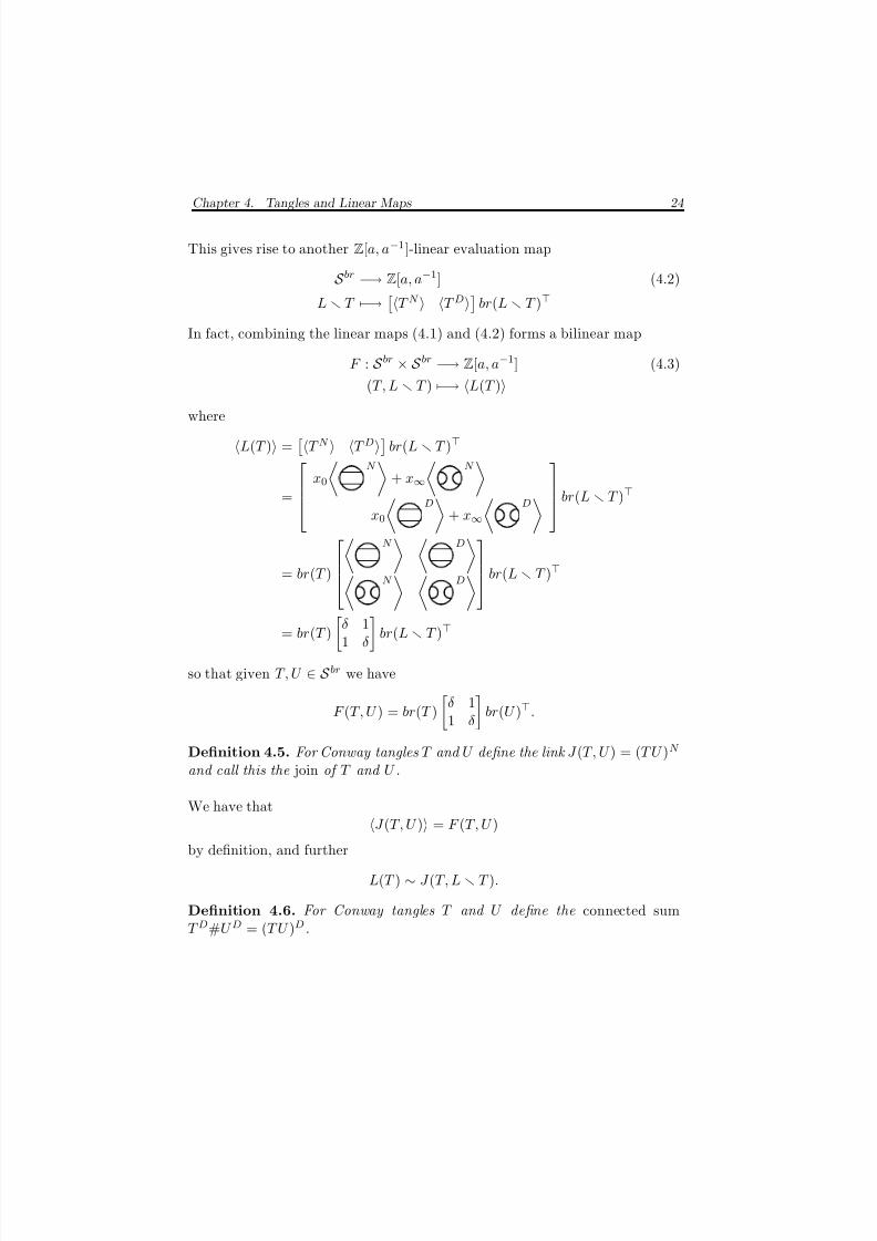
In fact, combining the linear maps (4.1) and (4.2) forms a bilinear map
F : S br × S br −→ Z[a, a−1] (4.3)
(T, L T ) −→ L(T )where
L(T ) =T N T D br(L T )
=
x0
N
+ x∞
N
x0
D
+ x∞
D br(L T )
= br(T )
N
D
N
D
br(L T )
= br(T )
δ 11 δ
br(L T )
so that given T, U ∈ S br we have
F (T, U ) = br(T )
δ 11 δ
br(U ).
Definition 4.5. For Conway tangles T and U define the link J (T, U ) = (T U )N
and call this the join of T and U .
We have that J (T, U ) = F (T, U )
by definition, and further
L(T ) ∼ J (T, L T ).
Definition 4.6. For Conway tangles T and U define the connected sumT D#U D = (T U )D.
8/3/2019 Liam Thomas Watson- Knots, Tangles and Braid Actions
http://slidepdf.com/reader/full/liam-thomas-watson-knots-tangles-and-braid-actions 33/82
Chapter 4. Tangles and Linear Maps 25
Since any link L may be written as T D for some tangle T this definition givesrise to a connected sum for links. It follows that
L1#L2 = L1L2,
andV L1#L2 = V L1V L2
provided orientations agree. A similar argument gives such an equality for theHOMFLY polynomial, and hence the Alexander polynomial as well.
4.2 Conway Mutation
Consider a link diagram containing some Conway tangle T . We can choosethe coordinate system so that T is contained in the unit disk, for convenienceof notation. Further, we can arrange that the 4 points of intersection betweenthe link and the boundary of the disk are
± 1√2
, ± 1√2
, 0
.
Let ρ be a 180 degree rotation of the unit disk about any of the three coor-
dinate axis. Note that ρ leaves the external wiring unchanged and, for such aprojection, ρ fixes the boundary points as a set.
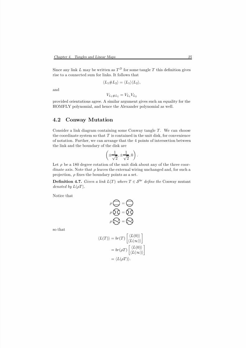
Definition 4.7. Given a link L(T ) where T ∈ S br define the Conway mutantdenoted by L(ρT ).
Notice that
ρ =
ρ =
ρ =
so that
L(T ) = br(T )
L(0)L(∞)
= br(ρT )
L(0)L(∞)
= L(ρT ).
8/3/2019 Liam Thomas Watson- Knots, Tangles and Braid Actions
http://slidepdf.com/reader/full/liam-thomas-watson-knots-tangles-and-braid-actions 34/82
Chapter 4. Tangles and Linear Maps 26
Moreover, with orientation dictated by the external wiring
w(T ) = w(ρT )
so we have the following theorem.
Theorem 4.8. V L(T ) = V L(ρT ).
While it may be that L(T ) L(ρT ), it is certain that this method does notprovide an answer to question 3.2: It can be shown that a Conway mutant of the unknot is always unknotted [30]. Theorem 4.8 is in fact a corollary of a
stronger statement.
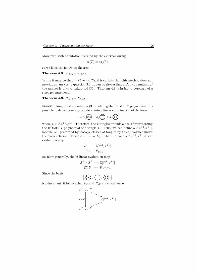
Theorem 4.9. P L(T ) = P L(ρT ).
proof. Using the skein relation (3.6) defining the HOMFLY polynomial, it ispossible to decompose any tangle T into a linear combination of the form
T = a1 + a2 + a3
where ai ∈ Z[t±1, x±1]. Therefore, these tangles provide a basis for presentingthe HOMFLY polynomial of a tangle T . Thus, we can define a Z[t±1, x±1]-module S P generated by isotopy classes of tangles up to equivalence under
the skein relation. Moreover, if L = L(T ) then we have a Z[t±1
, x±1
]-linearevaluation map
S P −→ Z[t±1, x±1]
T −→ P L(T )
or, more generally, the bi-linear evaluation map
S P × S P −→ Z[t±1, x±1]
(T, U ) −→ P J (T,U ).
Since the basis
, ,
is ρ-invariant, it follows that P T and P ρT are equal hence
S P × S P
ρ×id
( ( R R R R R R R R
Z[t±1, x±1]
S P × S P 6 6 l l l l l l l l
8/3/2019 Liam Thomas Watson- Knots, Tangles and Braid Actions
http://slidepdf.com/reader/full/liam-thomas-watson-knots-tangles-and-braid-actions 35/82
Chapter 4. Tangles and Linear Maps 27
commutes andP L(T ) = P L(ρT ).
4.3 The Skein Module
Everything that has been said regarding tangles to this point can be stated ina more general setting [30, 31].
Definition 4.10. Given a link L in S3 consider a 3-ball B3 ⊂ S3 such that ∂B3 intersects L in exactly 2n points. The intersection B3 ∩ L is called an n-tangle denoted by T . As before, the exterior of the n-tangle S3 B3 ∩ L isanother n-tangle L T called an external wiring.
In this setting, Conway tangles arise for n = 2 as 2-tangles.
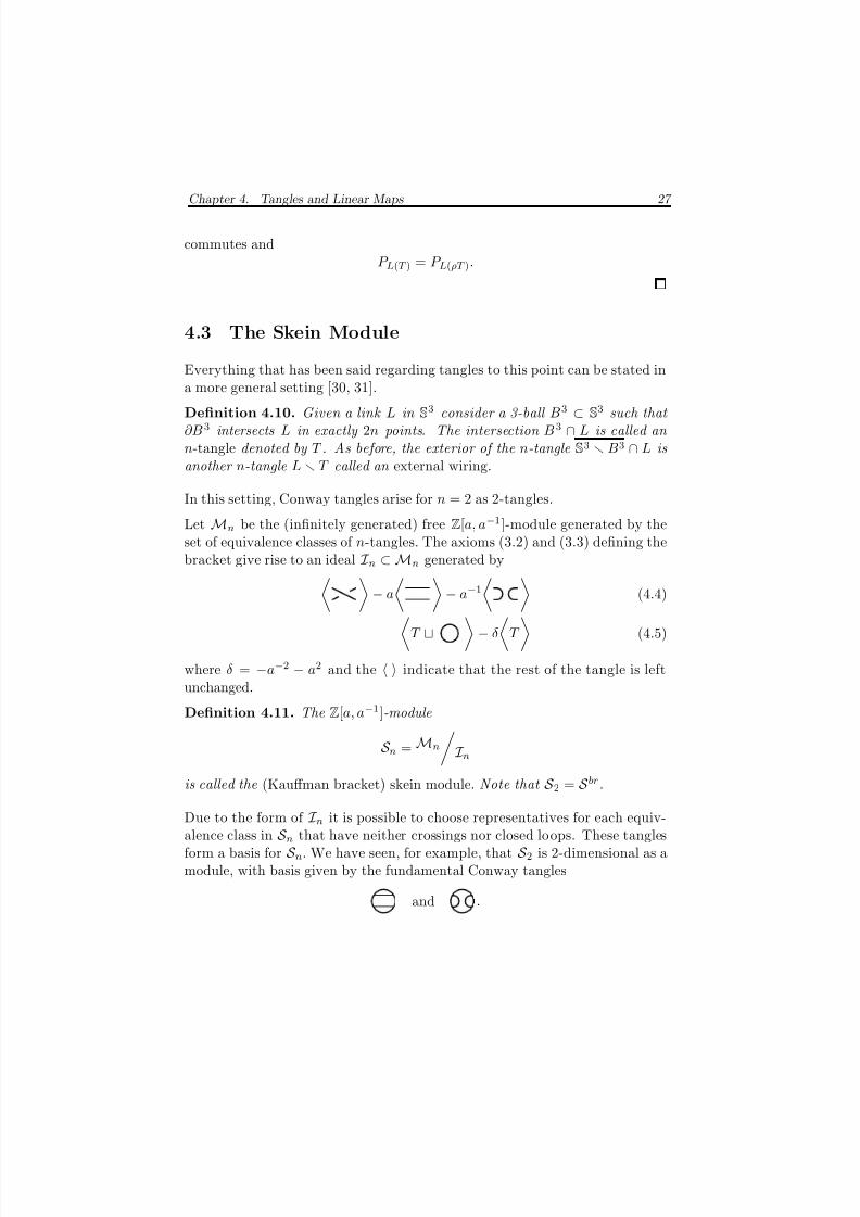
Let Mn be the (infinitely generated) free Z[a, a−1]-module generated by theset of equivalence classes of n-tangles. The axioms (3.2) and (3.3) defining thebracket give rise to an ideal I n ⊂ Mn generated by
− a − a−1 (4.4)
T
− δ
T
(4.5)
where δ = −a−2 − a2 and the indicate that the rest of the tangle is leftunchanged.
Definition 4.11. The Z[a, a−1]-module
S n = Mn
I n
is called the (Kauffman bracket) skein module. Note that
S 2 =
S br.
Due to the form of I n it is possible to choose representatives for each equiv-alence class in S n that have neither crossings nor closed loops. These tanglesform a basis for S n. We have seen, for example, that S 2 is 2-dimensional as amodule, with basis given by the fundamental Conway tangles
and .
8/3/2019 Liam Thomas Watson- Knots, Tangles and Braid Actions
http://slidepdf.com/reader/full/liam-thomas-watson-knots-tangles-and-braid-actions 36/82
Chapter 4. Tangles and Linear Maps 28
Theorem 4.12. S n has dimension
C n =(2n)!
n!(n + 1)!
as a module.
proof. Simply put, we need to determine how many n-tangles there are thathave no crossings or closed loops. That is, given a disk in the plane with 2n
marked points on the boundary, how many ways can the points be connected
by non-intersecting arcs (up to isotopy)?
Clearly, C 1 = 1, and as discussed earlier C 2 = 2.
Now suppose n > 2 and consider a disk with 2n points on the boundary.Starting at some chosen boundary point and numbering clockwise, the pointlabeled 1 must connect to an even labeled point, say 2k. This arc divides thedisk in two: One disk having 2(k − 1) marked points, the other with 2(n − k).Therefore
C n =
nk=1
C k−1C n−k
= C 0C n−1 + C 1C n−2 + · · · + C n−1C 0
where C 0 = 1 by convention. Now consider the generating function
f (x) =∞i=0
C ixi
and notice
(f (x))2 =∞i=0
i
k=1
C k−1C n−k
xi
so thatx(f (x))2 = f (x)
−1
and
f (x) =1 − √
1 − 4x
2x.
To deduce the coefficients of f (x), first consider the expansion of √
z about 1.
√z =
∞i=0
di(z − 1)i
8/3/2019 Liam Thomas Watson- Knots, Tangles and Braid Actions
http://slidepdf.com/reader/full/liam-thomas-watson-knots-tangles-and-braid-actions 37/82
Chapter 4. Tangles and Linear Maps 29
where
di =
1 i = 0(−1)i−1(2i−3)!!
2ii! i > 0.
Therefore with z = 1 − 4x
√1 − 4x =
∞i=0
di(−4x)i
= 1 +∞
i=1
(
−1)i2i2idix
i
and
f (x) = − 1
2x
∞i=1
(−1)i2i2idixi
=∞i=1
(−1)i−12i2i−1dixi−1
so that
C i = (−1)i2i+12idi+1
= (−1)i
− 2i+1
2i (
−1)i(2i
−1)!!
2i+1(i + 1)!
=2i(2i − 1)!!
(i + 1)!
for i > 1. Finally, the fact that
2n(2n − 1)!!
(n + 1)!=
(2n)!
n!(n + 1)!
follows by induction since
2n+1(2(n + 1) − 1)!!
(n + 2)!=
2(2n + 1)
n + 2
2n(2n − 1)!!
(n + 1)!
= 2(n + 1)(2n + 1)(n + 2)(n + 1)
C n
=(2n + 2)(2n + 1)
(n + 2)(n + 1)
(2n)!
n!(n + 1)!
=(2(n + 1))!
(n + 1)!(n + 2)!.
8/3/2019 Liam Thomas Watson- Knots, Tangles and Braid Actions
http://slidepdf.com/reader/full/liam-thomas-watson-knots-tangles-and-braid-actions 38/82
Chapter 4. Tangles and Linear Maps 30
As an example of theorem 4.12, the 5-dimensional module S 3 has basis givenby
, , , ,
. (4.6)
Let a given n-tangle diagram be contained in the unit disk so that, of the2n boundary points, n have positive x-coordinate while the remaining n havenegative x-coordinate. With this special position, multiplication of tanglesby concatenation, as introduced for Conway tangles, extends to all n-tangles.
When two n-tangles are in fact n-braids, we are reduced to multiplication inBn. With this multiplication, S n has an algebra structure called the Temperly-Lieb algebra [21, 22].
The n-dimensional Temperly-Lieb algebra TLn over Z[a, a−1] has generatorse1, e2, . . . , en−1 and relations
e2i = δei (4.7)
eie j = e jei for |i − j| > 1 (4.8)
eie jei = ei for |i − j| = 1. (4.9)
The multiplicative identity for this algebra is exactly the identity in Bn, and
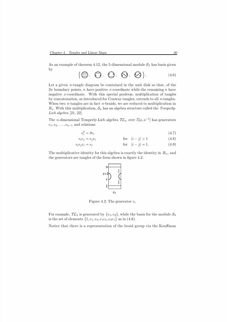
the generators are tangles of the form shown in figure 4.2.
¡
¡
¡
¢
£
¤ ¥ §
©
Figure 4.2: The generator ei
For example, TL3 is generated by {e1, e2}, while the basis for the module S 3is the set of elements {1, e1, e2, e1e2, e2e1} as in (4.6).
Notice that there is a representation of the braid group via the Kauffman
8/3/2019 Liam Thomas Watson- Knots, Tangles and Braid Actions
http://slidepdf.com/reader/full/liam-thomas-watson-knots-tangles-and-braid-actions 39/82
Chapter 4. Tangles and Linear Maps 31
bracket given by
Bn −→TLn
σi −→ a + a−1ei
σ−1i −→ aei + a−1.
4.4 Linear Maps
Let L = L(T 1, . . . , T k) be a link where {T i} is a collection of subtangles T i ⊂ L.If T i is a tangle such that T i = T i as elements of S n then, in the most generalsetting, L = L(T 1, . . . , T k) is a mutant of L (relative to the Kauffman bracket).Therefore when w(L) = w(L), we have that
V L = V L .
Of course, it may be that L L and this approach has been used in attemptsto answer question 3.2 [30, 31].
Let’s first revisit Conway mutation in this context. We have, given the bilinearevaluation map F and a 180 degree rotation ρ, the commutative diagram
S 2 × S 2
ρ×id
F ( ( P P P
P P P P P
Z[a, a−1]
S 2 × S 2F
6 6 n n n n n n n n
since F = F ◦ (ρ × id). We saw that the linear transformation ρ was in factthe identity transformation on S 2, and as a result the link L = J (T, U ) andthe mutant L = J (ρ T,U ) have the same Kauffman bracket.
A possible generalization arises naturally at this stage. As was pointed outearlier, it is possible to construct a link from two tangles in many different andcomplicated ways. Starting with T ⊂ B3
T ⊂ S3 and U ⊂ B3
U ⊂ S3, the link
L(T, U ) is constructed by choosing an external wiring of S3
(B3T ∪ B3
U ). In
8/3/2019 Liam Thomas Watson- Knots, Tangles and Braid Actions
http://slidepdf.com/reader/full/liam-thomas-watson-knots-tangles-and-braid-actions 40/82
Chapter 4. Tangles and Linear Maps 32
this setting we have
L(T, U ) = br(T )
L(0, U )L(∞, U )
= br(T )
L(0, 0) L(0, ∞)L(∞, 0) L(∞, ∞)
br(U )
= br(T ) L br(U )
which gives rise to the bilinear map
G : S 2 × S 2 −→ Z[a, a−1]
(T, U ) −→ br(T ) L br(U ).
If additionally there is a linear transformation
τ : S 2 × S 2 −→ S 2 × S 2(T, U ) −→ (τ 1T, τ 2U )
which acts as the identity as a linear transformation of modules, then we havethe commutative diagram
S 2 × S 2
τ =τ 1×τ 2
G ( ( P P P
P P P P P
Z[a, a−1]
S 2 × S 2G
6 6 n n n n n n n n
and finally, if w(L(T, U )) = w(L(τ 1T, τ 2U )) we can conclude that
V L(T,U ) = V L(τ 1T,τ 2U ).
4.5 Braid Actions
The three strand braid group has presentation
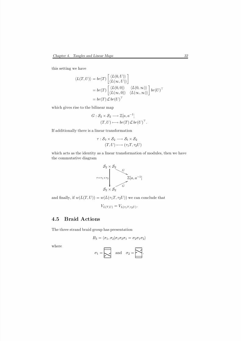
B3 = σ1, σ2|σ1σ2σ1 = σ2σ1σ2where
σ1 = and σ2 = .

8/3/2019 Liam Thomas Watson- Knots, Tangles and Braid Actions
http://slidepdf.com/reader/full/liam-thomas-watson-knots-tangles-and-braid-actions 41/82
Chapter 4. Tangles and Linear Maps 33
¡
Figure 4.3: The tangle T β ∈ S 2
Given T ∈ S 2 and a β ∈ B3 we can define a new 2-tangle denoted T β as infigure 4.3.
Proposition 4.13. The map
S 2 × B3 −→ S 2(T, β ) −→ T β
is a well defined group action.
proof. Let idB3 be the identity braid. Then for any tangle T we have
T idB3 = T
since
¢
∼£
For β, β ∈ B3, the product ββ is defined by concatenation so that
(T
β
)
β
= T
ββ
by planar isotopy of the diagram
¤ ¥ ¦ §
8/3/2019 Liam Thomas Watson- Knots, Tangles and Braid Actions
http://slidepdf.com/reader/full/liam-thomas-watson-knots-tangles-and-braid-actions 42/82
Chapter 4. Tangles and Linear Maps 34
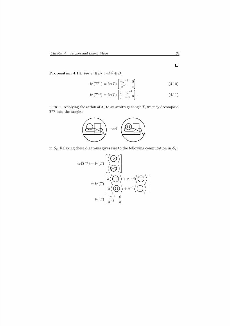
Proposition 4.14. For T ∈ S 2 and β ∈ B3
br(T σ1) = br(T )
−a−3 0a−1 a
(4.10)
br(T σ2) = br(T )
a a−1
0 −a−3
. (4.11)
proof. Applying the action of σ1 to an arbitrary tangle T , we may decomposeT σ1 into the tangles
and
in S 2. Relaxing these diagrams gives rise to the following computation in S 2:
br(T σ1) = br(T )
= br(T )
a
+ a−1δ
a
+ a−1
= br(T )
−a−3 0a−1 a
8/3/2019 Liam Thomas Watson- Knots, Tangles and Braid Actions
http://slidepdf.com/reader/full/liam-thomas-watson-knots-tangles-and-braid-actions 43/82
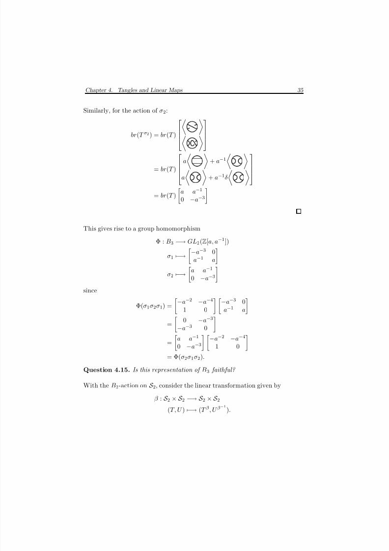
Chapter 4. Tangles and Linear Maps 35
Similarly, for the action of σ2:
br(T σ2) = br(T )
= br(T )
a
+ a−1
a + a
−1
δ
= br(T )
a a−1
0 −a−3
This gives rise to a group homomorphism
Φ : B3 −→ GL2(Z[a, a−1])
σ1 −→−a−3 0
a−1 a
σ2 −→ a a
−1
0 −a−3
since
Φ(σ1σ2σ1) =
−a−2 −a−4
1 0
−a−3 0a−1 a
=
0 −a−3
−a−3 0
=
a a−1
0 −a−3
−a−2 −a−4
1 0
= Φ(σ
2σ1
σ2
).
Question 4.15. Is this representation of B3 faithful?
With the B3-action on S 2, consider the linear transformation given by
β : S 2 × S 2 −→ S 2 × S 2(T, U ) −→ (T β , U β
−1
).
8/3/2019 Liam Thomas Watson- Knots, Tangles and Braid Actions
http://slidepdf.com/reader/full/liam-thomas-watson-knots-tangles-and-braid-actions 44/82
Chapter 4. Tangles and Linear Maps 36
For a link of the form L(T, U ), this leads to the definition of a new linkL(T β , U β
−1
).
Denote the evaluation matrix of L(T, U ) by
L =
L(0, 0) L(0, ∞)L(∞, 0) L(∞, ∞)
and suppose that L ∈ GL2(Z[a, a−1]), that is, det(L) = 0. Note that
L(T, U ) = br(T ) L br(U )
L(T β , U β −1
) = br(T )Φ(β ) L (Φ(β −1))br(U ).
So, defining a second B3-action
B3 × GL2(Z[a, a−1]) −→ GL2(Z[a, a−1])
(β, L) −→ Φ(β ) L (Φ(β −1)),
we are led to an algebraic question. When a non-trivial β ∈ B3 gives rise toa fixed point under this action, the linear transformation given by β is theidentity. Thus G = G
◦β and we have the commutative diagram
S 2 × S 2
β
G ( ( P P
P P P P P P
Z[a, a−1]
S 2 × S 2G
6 6 n n n n n n n n
where L ∈ Fix(β ), so that
L(T, U ) = L(T β , U β −1
).
In particular, we would like to study the case where
L(T, U ) L(T β , U β −1
).
Question 4.16. For a given link L(T, U ) with evaluation matrix L ∈ GL2(Z[a, a−1]),what are the elements β ∈ B3 such that L ∈ Fix(β )?
This question is the main focus of the following chapters.
8/3/2019 Liam Thomas Watson- Knots, Tangles and Braid Actions
http://slidepdf.com/reader/full/liam-thomas-watson-knots-tangles-and-braid-actions 45/82
Chapter 5
Kanenobu Knots
5.1 Construction
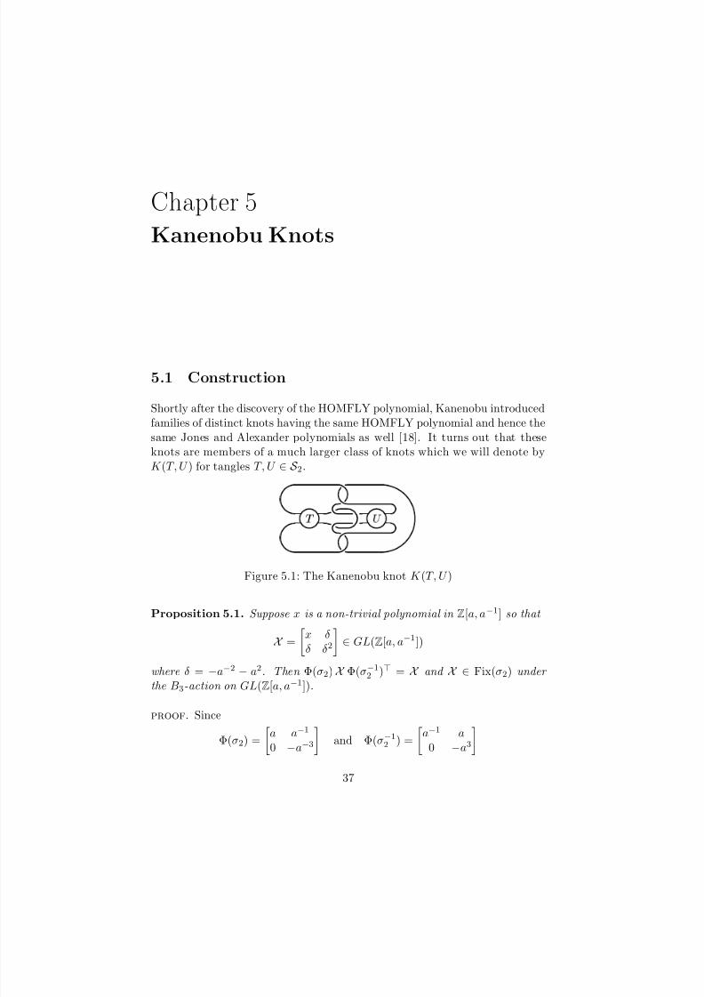
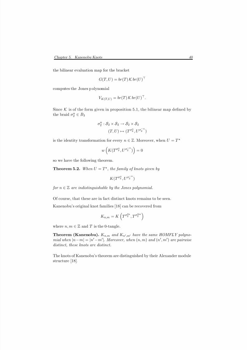
Shortly after the discovery of the HOMFLY polynomial, Kanenobu introducedfamilies of distinct knots having the same HOMFLY polynomial and hence thesame Jones and Alexander polynomials as well [18]. It turns out that theseknots are members of a much larger class of knots which we will denote byK (T, U ) for tangles T, U ∈ S 2.
¡
Figure 5.1: The Kanenobu knot K (T, U )
Proposition 5.1. Suppose x is a non-trivial polynomial in Z[a, a−1] so that
X =
x δ
δ δ2 ∈
GL(Z[a, a−1])
where δ = −a−2 − a2. Then Φ(σ2) X Φ(σ−12 ) = X and X ∈ Fix(σ2) under the B3-action on GL(Z[a, a−1]).
proof. Since
Φ(σ2) =
a a−1
0 −a−3
and Φ(σ−12 ) =
a−1 a
0 −a3
37
8/3/2019 Liam Thomas Watson- Knots, Tangles and Braid Actions
http://slidepdf.com/reader/full/liam-thomas-watson-knots-tangles-and-braid-actions 46/82
Chapter 5. Kanenobu Knots 38
we havea a−1
0 −a−3
x δ
δ δ2
a−1 0
a −a3
=
ax + a−1δ aδ + a−1δ2
−a−3δ −a−3δ2
a−1 0
a −a3
=
x + a−2δ + a2δ + δ2 −a4δ − a2δ2
−a−4δ − a−2δ2 δ2
=
x + δ(a−2 + a2 + δ) δ(−a4 − a2δ)
δ(−a−4 − a−2δ) δ2
= x δ(−
a4 + 1 + a4)δ(−a−4 + a−4 + 1) δ2
=
x δ
δ δ2
with δ = −a−2 − a2.
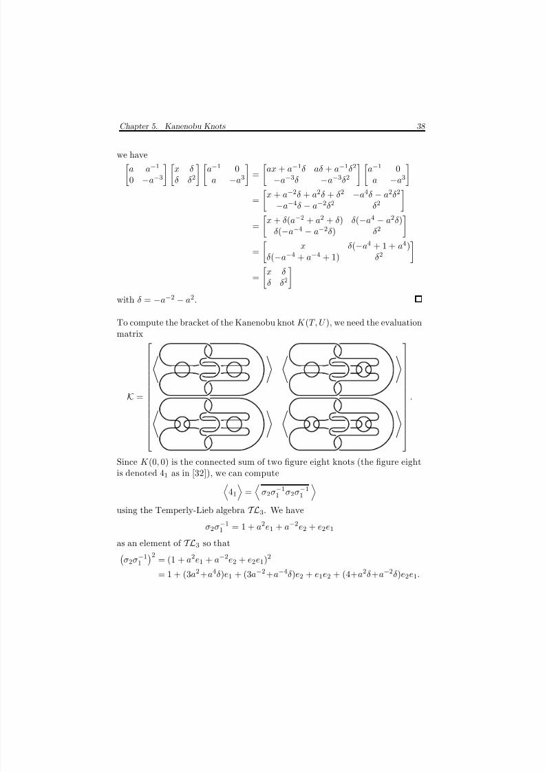
To compute the bracket of the Kanenobu knot K (T, U ), we need the evaluationmatrix
K =
.
Since K (0, 0) is the connected sum of two figure eight knots (the figure eightis denoted 41 as in [32]), we can compute
41
=
σ2σ−11 σ2σ−11 using the Temperly-Lieb algebra TL3. We have
σ2σ−11 = 1 + a2e1 + a−2e2 + e2e1
as an element of TL3 so thatσ2σ−11
2= (1 + a2e1 + a−2e2 + e2e1)2
= 1 + (3a2+a4δ)e1 + (3a−2+a−4δ)e2 + e1e2 + (4+a2δ+a−2δ)e2e1.
8/3/2019 Liam Thomas Watson- Knots, Tangles and Braid Actions
http://slidepdf.com/reader/full/liam-thomas-watson-knots-tangles-and-braid-actions 47/82
Chapter 5. Kanenobu Knots 39
Then the Kauffman bracket is given byσ2σ−11
2= δ2 + (3a2 + a4δ)δ + (3a−2 + a−4δ)δ + 1 + (4 + a2δ + a−2δ)(1)
= δ(−a−6 + 2a−4 + 2a4 − a6) + 5
= a−8 − a−4 + 1 − a4 + a8
and
41#41
= a−8
−a−4 + 1
−a4 + a8
2
= a−16 − 2a−12 + 3a−8 − 4a−4 + 5 − 4a4 + 3a8 − 2a12 + a16.
In addition, it can be seen from the braid closure σ2σ−11 σ2σ−11 ∼ 41 thatw(41) = 0 and hence
w (K (0, 0)) = w(41#41) = 0.
Thus the Jones polynomial of K (0, 0) is given by
V K (0,0) = a−16 − 2a−12 + 3a−8 − 4a−4 + 5 − 4a4 + 3a8 − 2a12 + a16.
Now the evaluation matrix for K (T, U ) is given by
K =
(a−8 − a−4 + 1 − a4 + a8)2 δ
δ δ2
since the three entries for K (0, ∞), K (∞, 0) and K (∞, ∞) are all equivalent tounlinks with no crossings via applications of the Reidemeister move R 2 (recallthat R2 leaves the Kauffman bracket unchanged).
For any tangle diagram T , denote by T the tangle diagram obtained by switch-ing each crossing of T . That is, for any choice of orientation
w(T ) = −w(T ).
This can be extended to knot diagrams K , where K is the diagram such that
w(K ) = −w(K )
so that K is the mirror image of K .
When U = T ,w(K (T, U )) = 0
8/3/2019 Liam Thomas Watson- Knots, Tangles and Braid Actions
http://slidepdf.com/reader/full/liam-thomas-watson-knots-tangles-and-braid-actions 48/82
Chapter 5. Kanenobu Knots 40
the bilinear evaluation map for the bracket
G(T, U ) = br(T ) K br(U )
computes the Jones polynomial
V K (T,U ) = br(T ) K br(U ).
Since
Kis of the form given in proposition 5.1, the bilinear map defined by
the braid σn2 ∈ B3
σn2 : S 2 × S 2 → S 2 × S 2(T, U ) → (T σ
n
2 , U σ−n
2 )
is the identity transformation for every n ∈ Z. Moreover, when U = T
w
K (T σn
2 , U σ−n
2 )
= 0
so we have the following theorem.
Theorem 5.2. When U = T , the family of knots given by
K (T σn
2 , U σ−n
2 )
for n ∈ Z are indistinguishable by the Jones polynomial.
Of course, that these are in fact distinct knots remains to be seen.
Kanenobu’s original knot families [18] can be recovered from
K n,m = K
T σ2n2 , T σ
2m2
where n, m
∈Z and T is the 0-tangle.
Theorem (Kanenobu). K n,m and K n,m have the same HOMFLY polyno-mial when |n−m| = |n−m|. Moreover, when (n, m) and (n, m) are pairwisedistinct, these knots are distinct.
The knots of Kanenobu’s theorem are distinguished by their Alexander modulestructure [18].
8/3/2019 Liam Thomas Watson- Knots, Tangles and Braid Actions
http://slidepdf.com/reader/full/liam-thomas-watson-knots-tangles-and-braid-actions 49/82
Chapter 5. Kanenobu Knots 41
5.2 Basic Examples
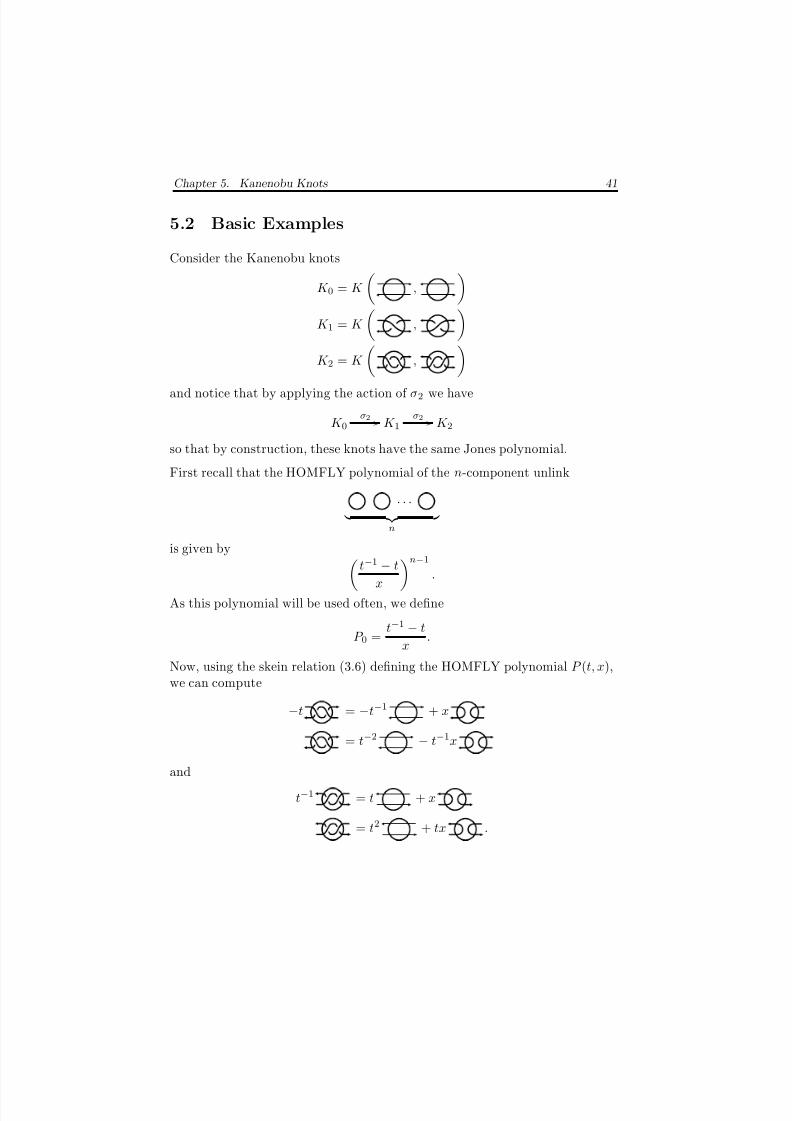
Consider the Kanenobu knots
K 0 = K
,
K 1 = K
,
K 2 = K , and notice that by applying the action of σ2 we have
K 0σ2 / / K 1
σ2 / / K 2
so that by construction, these knots have the same Jones polynomial.
First recall that the HOMFLY polynomial of the n-component unlink
· · ·
n
is given by t−1 − t
x
n−1.
As this polynomial will be used often, we define
P 0 =t−1 − t
x.
Now, using the skein relation (3.6) defining the HOMFLY polynomial P (t, x),we can compute
−t = −t−1 + x
= t−2 − t−1x
and
t−1 = t + x
= t2 + tx .
8/3/2019 Liam Thomas Watson- Knots, Tangles and Braid Actions
http://slidepdf.com/reader/full/liam-thomas-watson-knots-tangles-and-braid-actions 50/82
Chapter 5. Kanenobu Knots 42
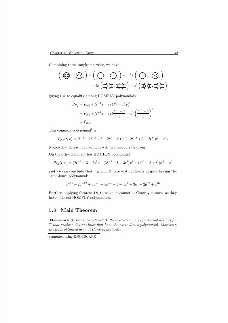
Combining these tangles pairwise, we have,
=
,
+ t−1x
,
− tx
,
− x2
,
giving rise to equality among HOMFLY polynomials
P K 2 = P K 0 + (t
−1
x − tx)P 0 − x
2
P
2
0
= P K 0 + (t−1x − tx)t−1 − t
x− x2
t−1 − t
x
2
= P K 0 .
This common polynomial1 is
P K 0(t, x) = (t−4 − 2t−2 + 3 − 2t2 + t4) + (−2t−2 + 2 − 2t2)x2 + x4.
Notice that this is in agreement with Kanenobu’s theorem.
On the other hand K 1 has HOMFLY polynomial
P K 1(t, x) = (2t−2 − 3 + 2t2) + (3t−2 − 8 + 3t2)x2 + (t−2 − 5 + t2)x4 − x6
and we can conclude that K 0 and K 1 are distinct knots despite having thesame Jones polynomial:
a−16 − 2a−12 + 3a−8 − 4a−4 + 5 − 4a4 + 3a8 − 2a12 + a16
Further, applying theorem 4.9, these knots cannot be Conway mutants as theyhave different HOMFLY polynomials.
5.3 Main Theorem
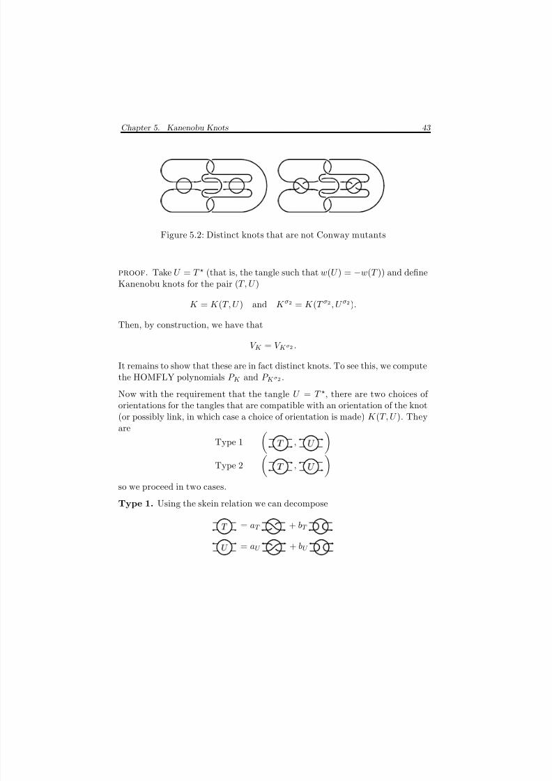
Theorem 5.3. For each 2-tangle T there exists a pair of external wirings for T that produce distinct links that have the same Jones polynomial. Moreover,the links obtained are not Conway mutants.
1computed using KNOTSCAPE
8/3/2019 Liam Thomas Watson- Knots, Tangles and Braid Actions
http://slidepdf.com/reader/full/liam-thomas-watson-knots-tangles-and-braid-actions 51/82
Chapter 5. Kanenobu Knots 43
Figure 5.2: Distinct knots that are not Conway mutants
proof. Take U = T (that is, the tangle such that w(U ) = −w(T )) and defineKanenobu knots for the pair (T, U )
K = K (T, U ) and K σ2 = K (T σ2 , U σ2).
Then, by construction, we have that
V K = V K σ2 .
It remains to show that these are in fact distinct knots. To see this, we computethe HOMFLY polynomials P K and P K σ2 .
Now with the requirement that the tangle U = T , there are two choices of orientations for the tangles that are compatible with an orientation of the knot(or possibly link, in which case a choice of orientation is made) K (T, U ). Theyare
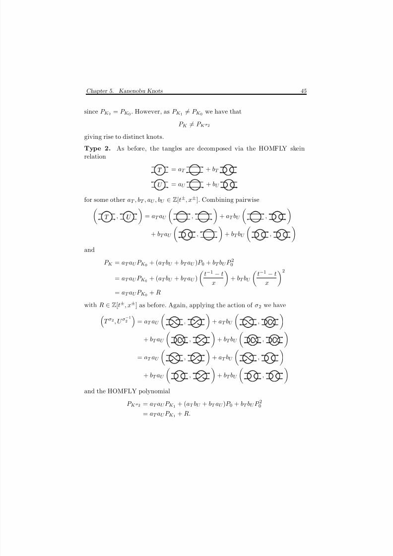
Type 1
, ¡
Type 2
¢ ,
£
so we proceed in two cases.
Type 1. Using the skein relation we can decompose
¤ = aT + bT
¥ = aU + bU

8/3/2019 Liam Thomas Watson- Knots, Tangles and Braid Actions
http://slidepdf.com/reader/full/liam-thomas-watson-knots-tangles-and-braid-actions 52/82
Chapter 5. Kanenobu Knots 44
where aT , bT , aU , bU ∈ Z[t±, x±]. Combining pairwise we obtain , ¡
= aT aU
,
+ aT bU
,
+ bT aU
,
+ bT bU
,
so that
P K = aT aU P K 1 + (aT bU + bT aU )P 0 + bT bU P 2
0
= aT aU P K 1 + (aT bU + bT aU )
t−1 − t
x
+ bT bU
t−1 − t
x
2
= aT aU P K 1 + R
where R = (aT bU + bT aU )t−1−tx
+ bT bU
t−1−tx
2. Now applying the action
of σ2 we have
T σ2 =¢
and U σ−12 =
£
thereforeT σ2, U σ
−12
= aT aU
,
+ aT bU
,
+ bT aU
,
+ bT bU
,
= aT aU
,
+ aT bU
,
+ bT aU , + bT bU ,
so that
P K σ2 = aT aU P K 2 + (aT bU + bT aU )P 0 + bT bU P 20
= P K 0 + R
8/3/2019 Liam Thomas Watson- Knots, Tangles and Braid Actions
http://slidepdf.com/reader/full/liam-thomas-watson-knots-tangles-and-braid-actions 53/82
Chapter 5. Kanenobu Knots 45
since P K 2 = P K 0 . However, as P K 1 = P K 0 we have that
P K = P K σ2
giving rise to distinct knots.
Type 2. As before, the tangles are decomposed via the HOMFLY skeinrelation
= aT + bT
¡
= aU + bU
for some other aT , bT , aU , bU ∈ Z[t±, x±]. Combining pairwise¢ , £
= aT aU
,
+ aT bU
,
+ bT aU
,
+ bT bU
,
and
P K = aT aU P K 0 + (aT bU + bT aU )P 0 + bT bU P 20
= aT aU P K 0 + (aT bU + bT aU ) t−1 − t
x+ bT bU
t−1 − tx
2
= aT aU P K 0 + R
with R ∈ Z[t±, x±] as before. Again, applying the action of σ2 we haveT σ2, U σ
−12
= aT aU
,
+ aT bU
,
+ bT aU
,
+ bT bU
,
= aT aU , + aT bU ,
+ bT aU
,
+ bT bU
,
and the HOMFLY polynomial
P K σ2 = aT aU P K 1 + (aT bU + bT aU )P 0 + bT bU P 20
= aT aU P K 1 + R.
8/3/2019 Liam Thomas Watson- Knots, Tangles and Braid Actions
http://slidepdf.com/reader/full/liam-thomas-watson-knots-tangles-and-braid-actions 54/82
Chapter 5. Kanenobu Knots 46
Once again, as P K 1 = P K 0 we have that
P K = P K σ2
giving rise to distinct knots.
Finally, as K and K σ2 have distinct HOMFLY polynomials in both cases, itfollows from theorem 4.9 that these knots cannot be Conway mutants.
5.4 Examples
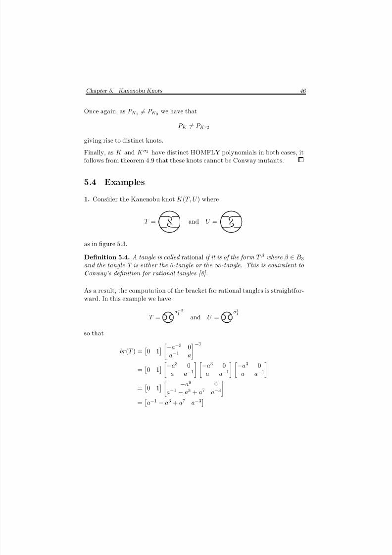
1. Consider the Kanenobu knot K (T, U ) where
T = and U =
as in figure 5.3.
Definition 5.4. A tangle is called rational if it is of the form T β where β ∈ B3
and the tangle T is either the 0-tangle or the
∞-tangle. This is equivalent to
Conway’s definition for rational tangles [8].
As a result, the computation of the bracket for rational tangles is straightfor-ward. In this example we have
T =σ−31
and U =σ31
so that
br(T ) =
0 1
−a−3 0
a−1 a
−3=
0 1 −a3 0
a a−1−a3 0
a a−1 −a3 0
a a−1
=
0 1 −a9 0
a−1 − a3 + a7 a−3
=
a−1 − a3 + a7 a−3
8/3/2019 Liam Thomas Watson- Knots, Tangles and Braid Actions
http://slidepdf.com/reader/full/liam-thomas-watson-knots-tangles-and-braid-actions 55/82
Chapter 5. Kanenobu Knots 47
and
br(U ) =
0 1 −a−3 0
a−1 a
3=
0 1 −a−3 0
a−1 a
−a−3 0a−1 a
−a−3 0a−1 a
=
a−7 − a−1 + a a3
.
Now
K (T, U ) = br(T ) K br(U )
= br(T )
(a−8 − a−4 + 1 − a4 + a8)2 −a−2 − a2
−a−2 − a2 a−4 + 2 + a4
br(U )
= a−24 − 4a−20 + 10a−16 − 19a−12 + 27a−8 − 33a−4
+ 37 − 33a4 + 27a8 − 19a12 + 10a16 − 4a20 + a24
hence
V K (T,U ) =a−24 − 4a−20 + 10a−16 − 19a−12 + 27a−8 − 33a−4
+ 37−
33a4 + 27a8
−19a12 + 10a16
−4a20 + a24.
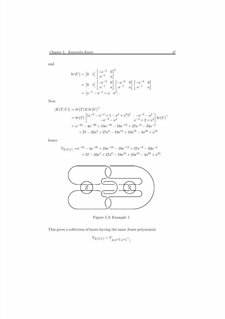
Figure 5.3: Example 1
This gives a collection of knots having the same Jones polynomial
V K (T,U ) = V K (T σ
n2 ,U σ
−n
2 )
8/3/2019 Liam Thomas Watson- Knots, Tangles and Braid Actions
http://slidepdf.com/reader/full/liam-thomas-watson-knots-tangles-and-braid-actions 56/82
Chapter 5. Kanenobu Knots 48
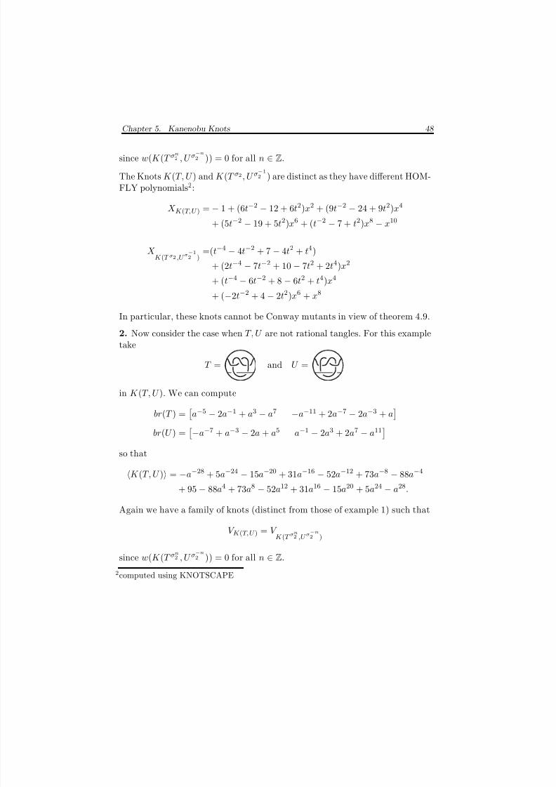
since w(K (T σn
2 , U σ−n
2 )) = 0 for all n ∈ Z.
The Knots K (T, U ) and K (T σ2, U σ−12 ) are distinct as they have different HOM-
FLY polynomials2:
X K (T,U ) = − 1 + (6t−2 − 12 + 6t2)x2 + (9t−2 − 24 + 9t2)x4
+ (5t−2 − 19 + 5t2)x6 + (t−2 − 7 + t2)x8 − x10
X K (T
σ2 ,U
σ−1
2 )
=(t−4
−4t−2 + 7
−4t2 + t4)
+ (2t−4 − 7t−2 + 10 − 7t2 + 2t4)x2
+ (t−4 − 6t−2 + 8 − 6t2 + t4)x4
+ (−2t−2 + 4 − 2t2)x6 + x8
In particular, these knots cannot be Conway mutants in view of theorem 4.9.
2. Now consider the case when T, U are not rational tangles. For this exampletake
T = and U =
in K (T, U ). We can compute
br(T ) =
a−5 − 2a−1 + a3 − a7 −a−11 + 2a−7 − 2a−3 + a
br(U ) =−a−7 + a−3 − 2a + a5 a−1 − 2a3 + 2a7 − a11
so that
K (T, U ) = −a−28 + 5a−24 − 15a−20 + 31a−16 − 52a−12 + 73a−8 − 88a−4
+ 95 − 88a4 + 73a8 − 52a12 + 31a16 − 15a20 + 5a24 − a28.
Again we have a family of knots (distinct from those of example 1) such that
V K (T,U ) = V K (T σ
n2 ,U σ
−n
2 )
since w(K (T σn
2 , U σ−n
2 )) = 0 for all n ∈ Z.
2computed using KNOTSCAPE
8/3/2019 Liam Thomas Watson- Knots, Tangles and Braid Actions
http://slidepdf.com/reader/full/liam-thomas-watson-knots-tangles-and-braid-actions 57/82
Chapter 5. Kanenobu Knots 49
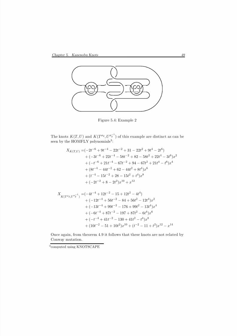
Figure 5.4: Example 2
The knots K (T, U ) and K (T σ2, U σ−12 ) of this example are distinct as can be
seen by the HOMFLY polynomials3:
X K (T,U ) =(−2t−6 + 9t−4 − 22t−2 + 31 − 22t2 + 9t4 − 2t6)
+ (−3t−6 + 22t−4 − 58t−2 + 82 − 58t2 + 22t4 − 3t6)x2
+ (−t
−6
+ 21t
−4
− 67t
−2
+ 94 − 67t
2
+ 21t
4
− t
6
)x
4
+ (8t−4 − 44t−2 + 62 − 44t2 + 8t4)x6
+ (t−4 − 15t−2 + 28 − 15t2 + t4)x8
+ (−2t−2 + 8 − 2t2)x10 + x12
X K (T σ2 ,U σ
−12 )
=(−4t−4 + 12t−2 − 15 + 12t2 − 4t4)
+ (−12t−4 + 56t−2 − 84 + 56t2 − 12t4)x2
+ (−13t−4 + 99t−2 − 176 + 99t2 − 13t4)x4
+ (−6t−4 + 87t−2 − 197 + 87t2 − 6t4)x6
+ (−t−4
+ 41t−2
− 130 + 41t2
− t4
)x8
+ (10t−2 − 51 + 10t2)x10 + (t−2 − 11 + t2)x12 − x14
Once again, from theorem 4.9 it follows that these knots are not related byConway mutation.
3computed using KNOTSCAPE
8/3/2019 Liam Thomas Watson- Knots, Tangles and Braid Actions
http://slidepdf.com/reader/full/liam-thomas-watson-knots-tangles-and-braid-actions 58/82
Chapter 5. Kanenobu Knots 50
5.5 Generalisation
We saw in proposition 5.1 under the action
B3 × GL2(Z[a, a−1]) −→ GL2(Z[a, a−1])
that x δ
δ δ2
∈ GL2
Z[a, a−1]
⊂ Fix(σ2).
As a final task for this chapter, we’ll define a family of links that generate suchevaluation matricies.
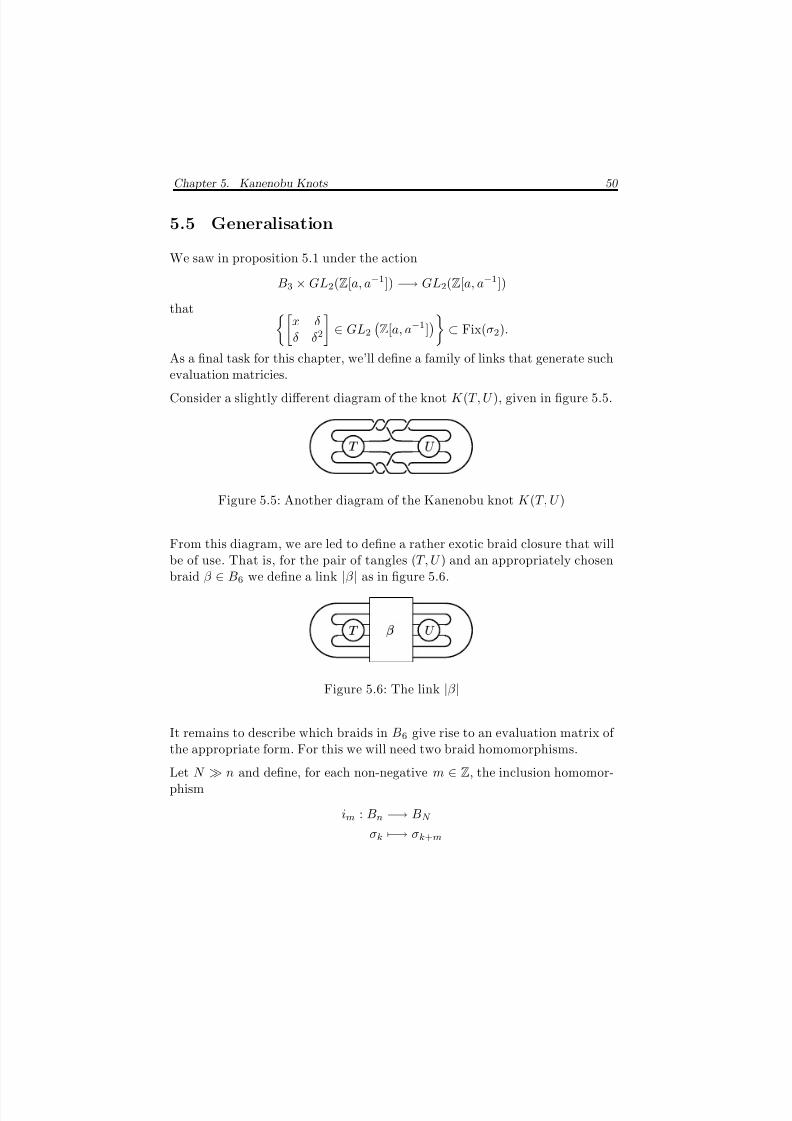
Consider a slightly different diagram of the knot K (T, U ), given in figure 5.5.
¡
Figure 5.5: Another diagram of the Kanenobu knot K (T, U )
From this diagram, we are led to define a rather exotic braid closure that willbe of use. That is, for the pair of tangles (T, U ) and an appropriately chosenbraid β ∈ B6 we define a link |β | as in figure 5.6.
¢
£ ¤
Figure 5.6: The link |β |
It remains to describe which braids in B6 give rise to an evaluation matrix of the appropriate form. For this we will need two braid homomorphisms.
Let N n and define, for each non-negative m ∈ Z, the inclusion homomor-phism
im : Bn −→ BN
σk −→ σk+m
8/3/2019 Liam Thomas Watson- Knots, Tangles and Braid Actions
http://slidepdf.com/reader/full/liam-thomas-watson-knots-tangles-and-braid-actions 59/82
Chapter 5. Kanenobu Knots 51
for each k ∈ {1, . . . , n− 1}. Note that when m = 0, this is reduces to thenatural inclusion Bn < BN . Now the group B3 ⊕ B3 arises as a subgroup of B6 by choosing
B3 ⊕ B3 −→ B6
(α, β ) −→ i0(α)i3(β ).
Notice that the image i0(α)i3(β ) contains no occurrence of the generator σ3
and hence
i0(α)i3(β ) = i3(β )i0(α)
in B6. Now define the switch homomorphism
s : B3 −→ B3
σ1 −→ σ−12
σ2 −→ σ−11
and note that, given a 180 degree rotation ρ in the projection plane, ρ(sβ ) =β −1.
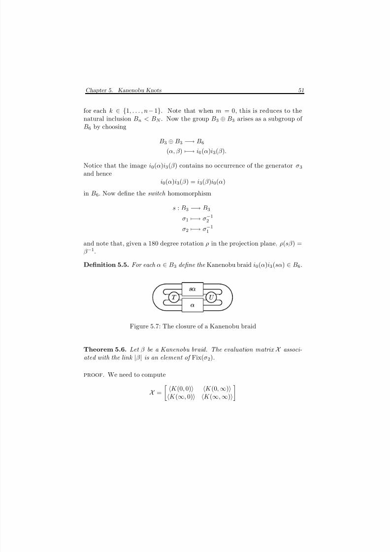
Definition 5.5. For each α
∈B3 define the Kanenobu braid i0(α)i3(sα)
∈B6.
¡ ¢
¤ ¥
Figure 5.7: The closure of a Kanenobu braid
Theorem 5.6. Let β be a Kanenobu braid. The evaluation matrix X associ-ated with the link
|β |
is an element of Fix(σ2
).
proof. We need to compute
X =
K (0, 0) K (0, ∞)K (∞, 0) K (∞, ∞)
8/3/2019 Liam Thomas Watson- Knots, Tangles and Braid Actions
http://slidepdf.com/reader/full/liam-thomas-watson-knots-tangles-and-braid-actions 60/82
Chapter 5. Kanenobu Knots 52
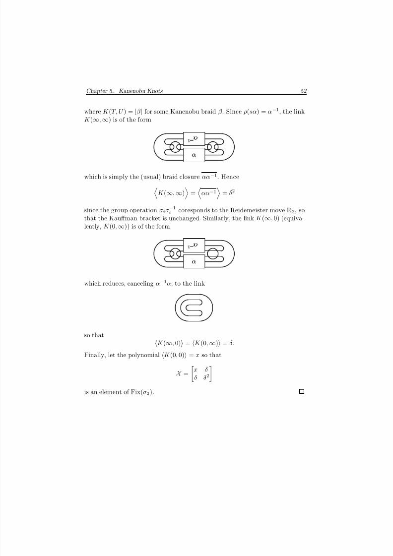
where K (T, U ) = |β | for some Kanenobu braid β . Since ρ(sα) = α−1, the linkK (∞, ∞) is of the form
¡
£
which is simply the (usual) braid closure αα−1. HenceK (∞, ∞)
=
αα−1
= δ2
since the group operation σiσ−1i coresponds to the Reidemeister move R2, so
that the Kauffman bracket is unchanged. Similarly, the link K (∞, 0) (equiva-lently, K (0, ∞)) is of the form
¤
¥
§
which reduces, canceling α−1α, to the link
so thatK (∞, 0) = K (0, ∞) = δ.
Finally, let the polynomial K (0, 0) = x so that
X =x δ
δ δ2
is an element of Fix(σ2).
8/3/2019 Liam Thomas Watson- Knots, Tangles and Braid Actions
http://slidepdf.com/reader/full/liam-thomas-watson-knots-tangles-and-braid-actions 61/82
Chapter 5. Kanenobu Knots 53
5.6 More Examples
For the following examples, we introduce the shorthand K (σ2, σ−12 ) referringto the knot obtained from the action
K (0, 0)σ2 / / K (σ2, σ−12 ).
We continue numbering of examples from section 5.4.
3. Taking the braid σ3
1σ−1
2σ1 ∈
B3
Figure 5.8: The braid σ31σ−12 σ1
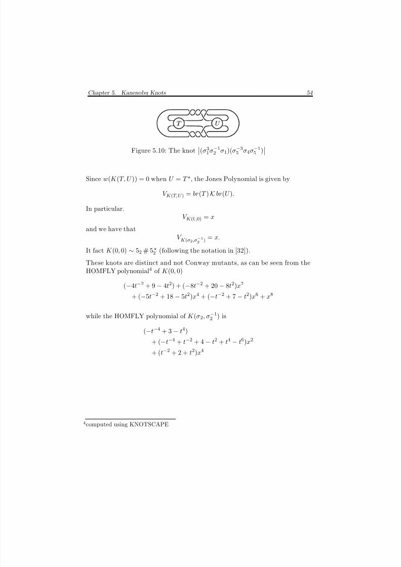
we can form the Kanenobu braid (σ31σ−12 σ1)(σ−35 σ4σ−15 ) ∈ B6
Figure 5.9: The Kanenobu braid (σ31σ−12 σ1)(σ−35 σ4σ−15 )
and the generalized Kanenobu knot
K (T, U ) =(σ3
1σ−12 σ1)(σ−35 σ4σ−15 ) .
K (T, U ) has evaluation matrix
K =x δ
δ δ2
where
x = − a−20 + 2a−16 − 4a−12 + 6a−8 − 7a−4
+ 9 − 7a4 + 6a8 − 4a12 + 2a16 − a20.
8/3/2019 Liam Thomas Watson- Knots, Tangles and Braid Actions
http://slidepdf.com/reader/full/liam-thomas-watson-knots-tangles-and-braid-actions 62/82
Chapter 5. Kanenobu Knots 54
¡
Figure 5.10: The knot(σ3
1σ−12 σ1)(σ−35 σ4σ−15 )
Since w(K (T, U )) = 0 when U = T , the Jones Polynomial is given by
V K (T,U ) = br(T ) K br(U ).
In particular,V K (0,0) = x
and we have thatV K (σ2,σ−12 ) = x.
It fact K (0, 0) ∼ 52 # 5 2 (following the notation in [32]).
These knots are distinct and not Conway mutants, as can be seen from theHOMFLY polynomial4 of K (0, 0)
(−4t−2 + 9 − 4t2) + (−8t−2 + 20 − 8t2)x2
+ (−5t−2 + 18 − 5t2)x4 + (−t−2 + 7 − t2)x6 + x8
while the HOMFLY polynomial of K (σ2, σ−12 ) is
(−t−4 + 3 − t4)
+ (−t−4 + t−2 + 4 − t2 + t4 − t6)x2
+ (t−2 + 2 + t2)x4
4computed using KNOTSCAPE
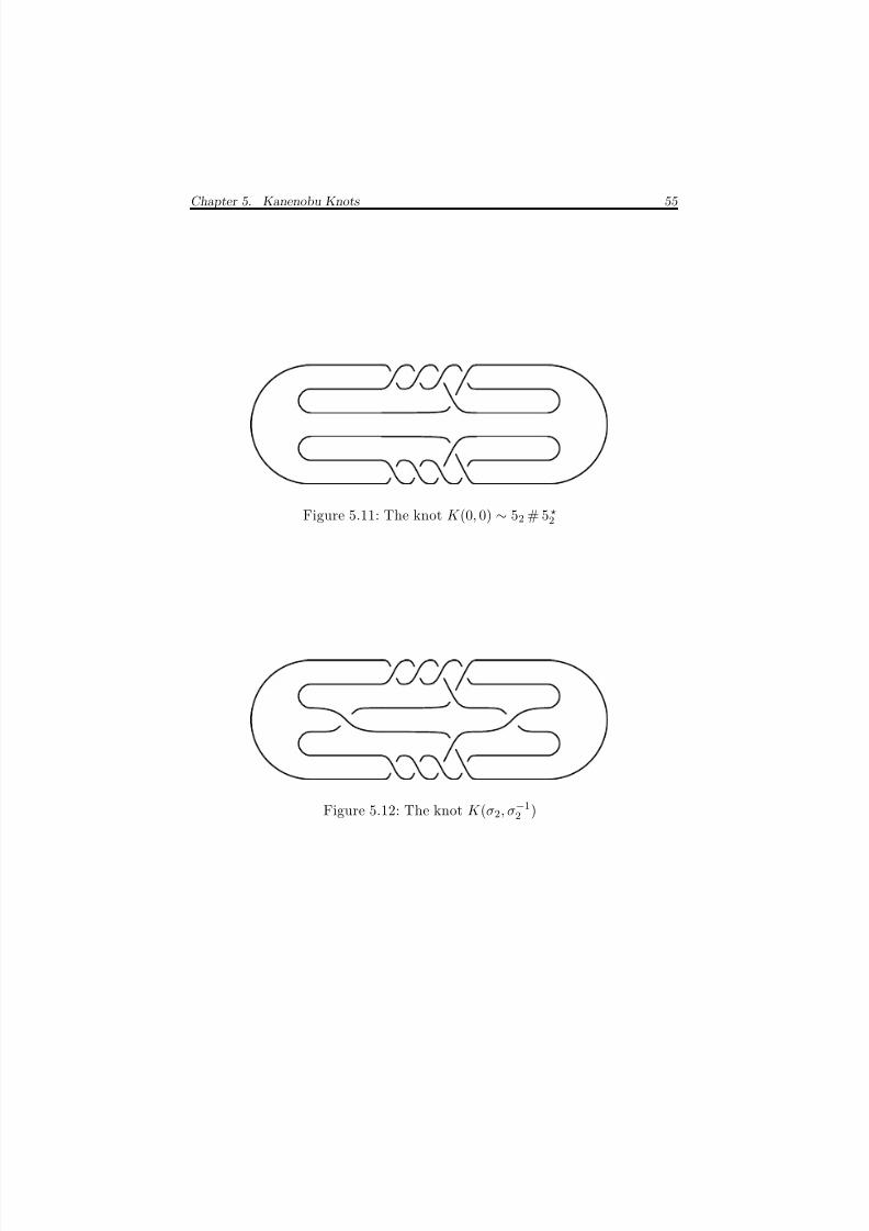
8/3/2019 Liam Thomas Watson- Knots, Tangles and Braid Actions
http://slidepdf.com/reader/full/liam-thomas-watson-knots-tangles-and-braid-actions 63/82
Chapter 5. Kanenobu Knots 55
Figure 5.11: The knot K (0, 0) ∼ 52 # 5 2
Figure 5.12: The knot K (σ2, σ−12 )
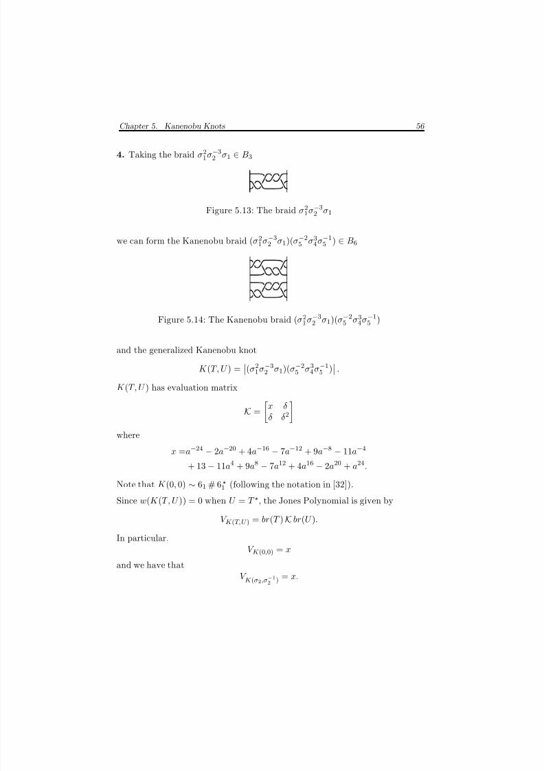
8/3/2019 Liam Thomas Watson- Knots, Tangles and Braid Actions
http://slidepdf.com/reader/full/liam-thomas-watson-knots-tangles-and-braid-actions 64/82
Chapter 5. Kanenobu Knots 56
4. Taking the braid σ21σ−32 σ1 ∈ B3
Figure 5.13: The braid σ21σ−32 σ1
we can form the Kanenobu braid (σ21σ−32 σ1)(σ−25 σ3
4σ−15 ) ∈ B6
Figure 5.14: The Kanenobu braid (σ21σ−32 σ1)(σ−25 σ3
4σ−15 )
and the generalized Kanenobu knot
K (T, U ) = (σ21σ−32 σ1)(σ−25 σ3
4σ−15 ) .
K (T, U ) has evaluation matrix
K =
x δ
δ δ2
where
x =a−24 − 2a−20 + 4a−16 − 7a−12 + 9a−8 − 11a−4
+ 13 − 11a4 + 9a8 − 7a12 + 4a16 − 2a20 + a24.
Note that K (0, 0) ∼ 61 # 6 1 (following the notation in [32]).
Since w(K (T, U )) = 0 when U = T
, the Jones Polynomial is given byV K (T,U ) = br(T ) K br(U ).
In particular,V K (0,0) = x
and we have thatV K (σ2,σ−12 ) = x.
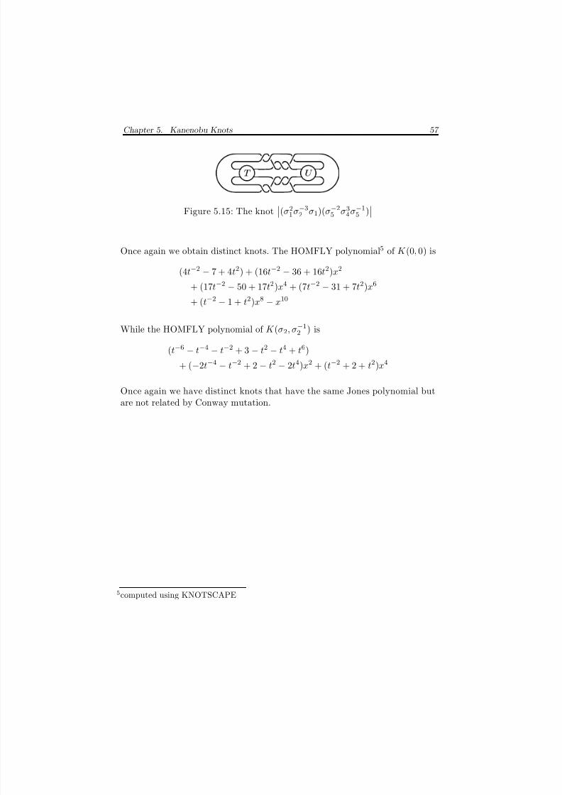
8/3/2019 Liam Thomas Watson- Knots, Tangles and Braid Actions
http://slidepdf.com/reader/full/liam-thomas-watson-knots-tangles-and-braid-actions 65/82
Chapter 5. Kanenobu Knots 57
¡
Figure 5.15: The knot(σ2
1σ−32 σ1)(σ−25 σ34σ−15 )
Once again we obtain distinct knots. The HOMFLY polynomial5 of K (0, 0) is
(4t−2 − 7 + 4t2) + (16t−2 − 36 + 16t2)x2
+ (17t−2 − 50 + 17t2)x4 + (7t−2 − 31 + 7t2)x6
+ (t−2 − 1 + t2)x8 − x10
While the HOMFLY polynomial of K (σ2, σ−12 ) is
(t−6 − t−4 − t−2 + 3 − t2 − t4 + t6)
+ (−2t−4 − t−2 + 2 − t2 − 2t4)x2 + (t−2 + 2 + t2)x4
Once again we have distinct knots that have the same Jones polynomial butare not related by Conway mutation.
5computed using KNOTSCAPE
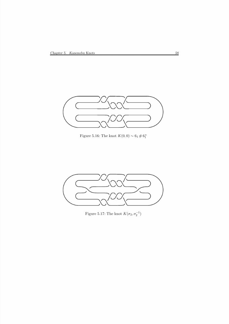
8/3/2019 Liam Thomas Watson- Knots, Tangles and Braid Actions
http://slidepdf.com/reader/full/liam-thomas-watson-knots-tangles-and-braid-actions 66/82
Chapter 5. Kanenobu Knots 58
Figure 5.16: The knot K (0, 0) ∼ 61 # 6 1
Figure 5.17: The knot K (σ2, σ−12 )
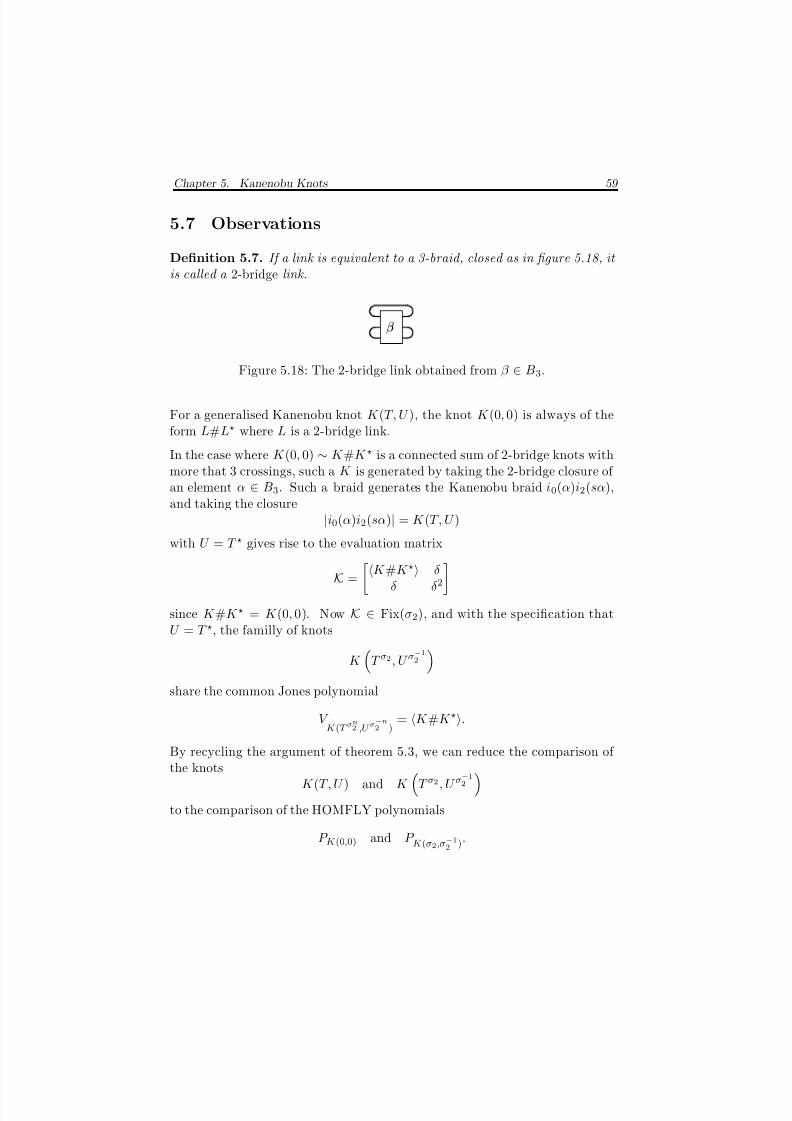
8/3/2019 Liam Thomas Watson- Knots, Tangles and Braid Actions
http://slidepdf.com/reader/full/liam-thomas-watson-knots-tangles-and-braid-actions 67/82
Chapter 5. Kanenobu Knots 59
5.7 Observations
Definition 5.7. If a link is equivalent to a 3-braid, closed as in figure 5.18, it is called a 2-bridge link.
Figure 5.18: The 2-bridge link obtained from β ∈ B3.
For a generalised Kanenobu knot K (T, U ), the knot K (0, 0) is always of theform L#L where L is a 2-bridge link.
In the case where K (0, 0) ∼ K #K is a connected sum of 2-bridge knots withmore that 3 crossings, such a K is generated by taking the 2-bridge closure of an element α ∈ B3. Such a braid generates the Kanenobu braid i0(α)i2(sα),and taking the closure
|i0(α)i2(sα)| = K (T, U )
withU
=T
gives rise to the evaluation matrix
K =
K #K δ
δ δ2
since K #K = K (0, 0). Now K ∈ Fix(σ2), and with the specification thatU = T , the familly of knots
K
T σ2, U σ−12
share the common Jones polynomial
V K (T σ
n2 ,U σ
−n
2 )=
K #K
.
By recycling the argument of theorem 5.3, we can reduce the comparison of the knots
K (T, U ) and K
T σ2, U σ−12
to the comparison of the HOMFLY polynomials
P K (0,0) and P K (σ2,σ−12 ).
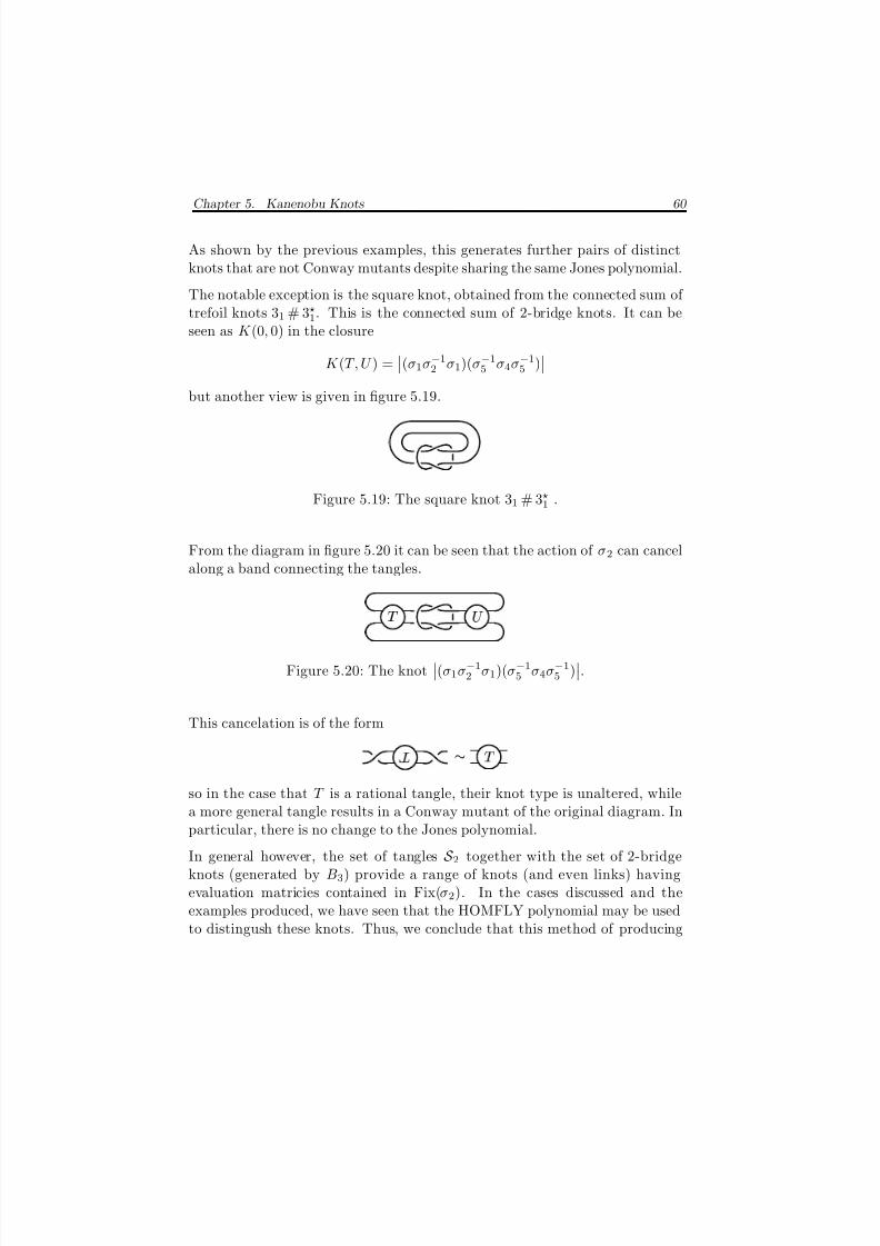
8/3/2019 Liam Thomas Watson- Knots, Tangles and Braid Actions
http://slidepdf.com/reader/full/liam-thomas-watson-knots-tangles-and-braid-actions 68/82
Chapter 5. Kanenobu Knots 60
As shown by the previous examples, this generates further pairs of distinctknots that are not Conway mutants despite sharing the same Jones polynomial.
The notable exception is the square knot, obtained from the connected sum of trefoil knots 31 # 31. This is the connected sum of 2-bridge knots. It can beseen as K (0, 0) in the closure
K (T, U ) =(σ1σ−12 σ1)(σ−15 σ4σ−15 )
but another view is given in figure 5.19.
Figure 5.19: The square knot 31 # 31 .
From the diagram in figure 5.20 it can be seen that the action of σ2 can cancelalong a band connecting the tangles.
¡
Figure 5.20: The knot(σ1σ−12 σ1)(σ−15 σ4σ−15 )
.This cancelation is of the form
¢
∼ £
so in the case that T is a rational tangle, their knot type is unaltered, while
a more general tangle results in a Conway mutant of the original diagram. Inparticular, there is no change to the Jones polynomial.
In general however, the set of tangles S 2 together with the set of 2-bridgeknots (generated by B3) provide a range of knots (and even links) havingevaluation matricies contained in Fix(σ2). In the cases discussed and theexamples produced, we have seen that the HOMFLY polynomial may be usedto distingush these knots. Thus, we conclude that this method of producing
8/3/2019 Liam Thomas Watson- Knots, Tangles and Braid Actions
http://slidepdf.com/reader/full/liam-thomas-watson-knots-tangles-and-braid-actions 69/82
Chapter 5. Kanenobu Knots 61
famillies knots sharing a common Jones polynomial is distinct from Conwaymutation.
In the next chapter, the results of Eliahou, Kauffman and Thistlethwaite [9]will be restated using the braid actions introduced in this paper.
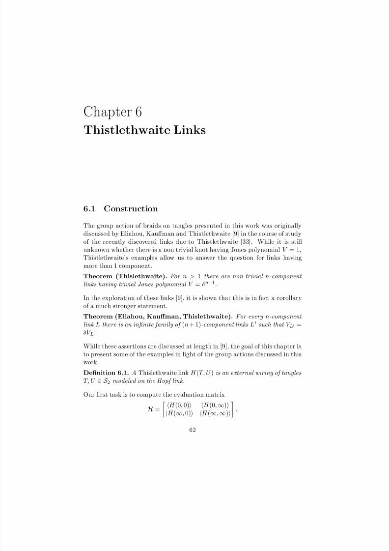
8/3/2019 Liam Thomas Watson- Knots, Tangles and Braid Actions
http://slidepdf.com/reader/full/liam-thomas-watson-knots-tangles-and-braid-actions 70/82
Chapter 6
Thistlethwaite Links
6.1 Construction
The group action of braids on tangles presented in this work was originallydiscussed by Eliahou, Kauffman and Thistlethwaite [9] in the course of studyof the recently discovered links due to Thistlethwaite [33]. While it is stillunknown whether there is a non trivial knot having Jones polynomial V = 1,Thistlethwaite’s examples allow us to answer the question for links havingmore than 1 component.
Theorem (Thislethwaite). For n > 1 there are non trivial n-component links having trivial Jones polynomial V = δn−1.
In the exploration of these links [9], it is shown that this is in fact a corollaryof a much stronger statement.
Theorem (Eliahou, Kauffman, Thislethwaite). For every n-component link L there is an infinite family of (n + 1)-component links L such that V L =δV L.
While these assertions are discussed at length in [9], the goal of this chapter isto present some of the examples in light of the group actions discussed in this
work.
Definition 6.1. A Thislethwaite link H (T, U ) is an external wiring of tanglesT, U ∈ S 2 modeled on the Hopf link.
Our first task is to compute the evaluation matrix
H =
H (0, 0) H (0, ∞)H (∞, 0) H (∞, ∞)
.
62
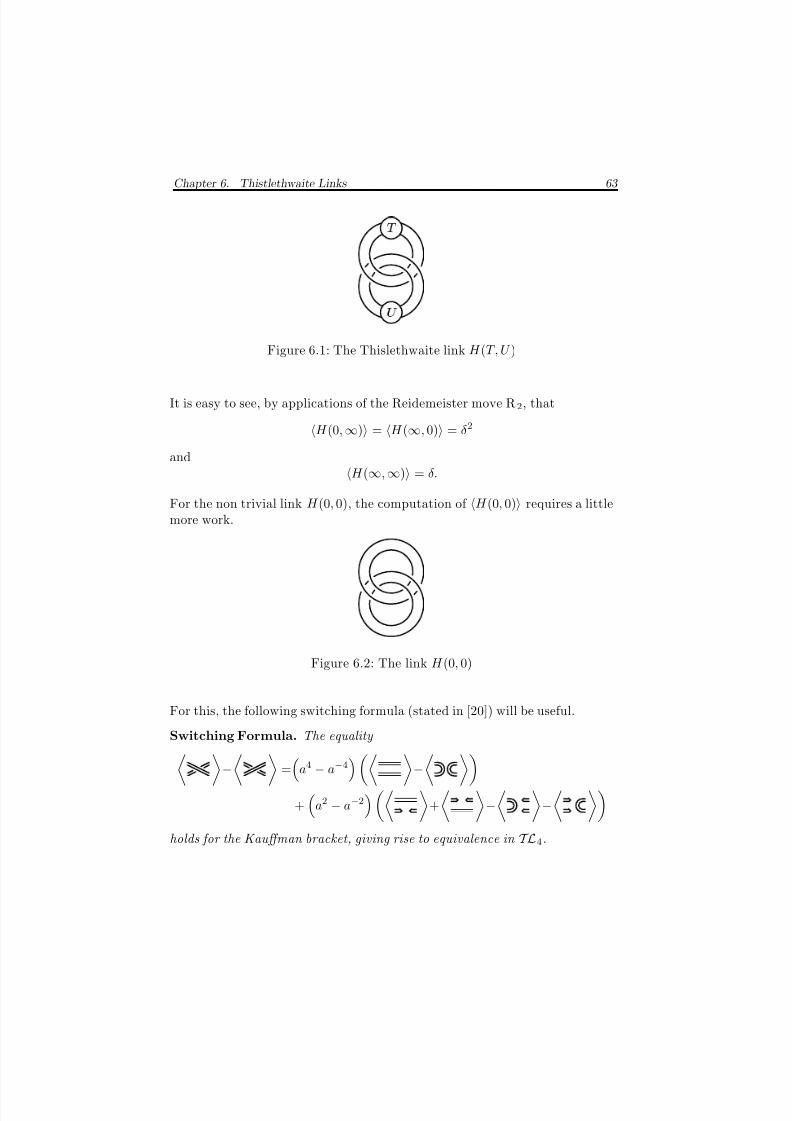
8/3/2019 Liam Thomas Watson- Knots, Tangles and Braid Actions
http://slidepdf.com/reader/full/liam-thomas-watson-knots-tangles-and-braid-actions 71/82
Chapter 6. Thistlethwaite Links 63
¡
Figure 6.1: The Thislethwaite link H (T, U )
It is easy to see, by applications of the Reidemeister move R 2, that
H (0, ∞) = H (∞, 0) = δ2
andH (∞, ∞) = δ.
For the non trivial link H (0, 0), the computation of H (0, 0) requires a littlemore work.
Figure 6.2: The link H (0, 0)
For this, the following switching formula (stated in [20]) will be useful.
Switching Formula. The equality −
=
a4 − a−4
−
+
a2 − a−2
+
−
−
holds for the Kauffman bracket, giving rise to equivalence in TL4.
8/3/2019 Liam Thomas Watson- Knots, Tangles and Braid Actions
http://slidepdf.com/reader/full/liam-thomas-watson-knots-tangles-and-braid-actions 72/82
Chapter 6. Thistlethwaite Links 64
proof of the switching formula. First note that the double crossingmay be viewed as the braid σ2σ1σ3σ2 ∈ B4. Thus, as
σi −→ a + a−1ei
gives a representation of the braid group in TLn, we can represent this elementof B4 as
(a2 + e1 + e2 + a−2e2e1)(a2 + e2 + e3 + a−2e3e2)
=a4 + a2e2 + a2e3 + e3e2
+ a2e1 + e1e2 + e1e3 + a−2e1e3e2
+ a2e2 + e22 + e2e3 + a−2e2e3e2
+ e2e1 + a−2e2e1e2 + a−2e2e1e3 + a−4e2e1e3e2
=a4 + a2e1 + (2a−2 + δ + 2a2)e2 + a2e3
+ a−2e1e3e2 + a−2e2e1e3 + a−4e2e1e3e2
+ e1e2 + e1e3 + e2e1 + e2e3 + e3e2.
Similarly, the double crossing may be viewed as (σ2σ1σ3σ2)−1 ∈ B4 sothat
σ−1i −→ a−1 + aei
gives the representation
(a−2 + e1 + e2 + a2e2e1)(a−2 + e2 + e3 + a2e3e2)
=a−4 + a−2e1 + (2a−2 + δ + 2a2)e2 + a−2e3
+ a2e1e3e2 + a2e2e1e3 + a4e2e1e3e2
+ e1e2 + e1e3 + e2e1 + e2e3 + e3e2.
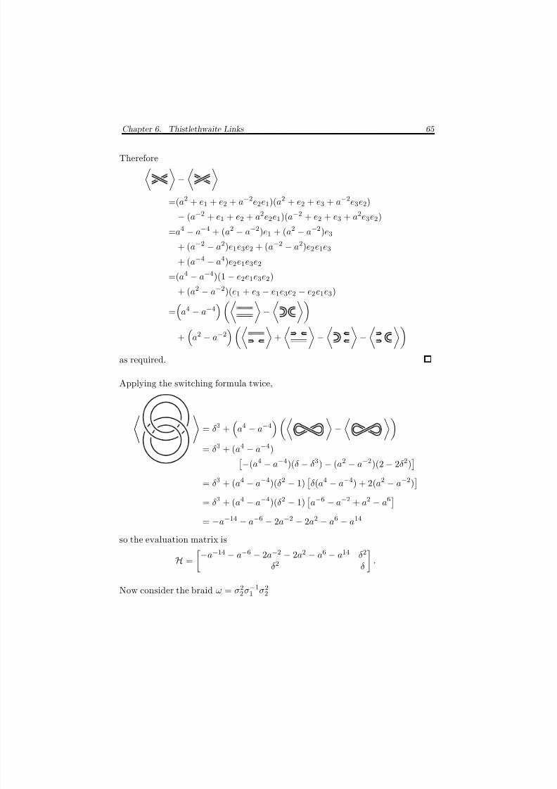
8/3/2019 Liam Thomas Watson- Knots, Tangles and Braid Actions
http://slidepdf.com/reader/full/liam-thomas-watson-knots-tangles-and-braid-actions 73/82
Chapter 6. Thistlethwaite Links 65
Therefore −
=(a2 + e1 + e2 + a−2e2e1)(a2 + e2 + e3 + a−2e3e2)
− (a−2 + e1 + e2 + a2e2e1)(a−2 + e2 + e3 + a2e3e2)
=a4 − a−4 + (a2 − a−2)e1 + (a2 − a−2)e3
+ (a−2
−a2)e1e3e2 + (a−2
−a2)e2e1e3
+ (a−4 − a4)e2e1e3e2
=(a4 − a−4)(1 − e2e1e3e2)
+ (a2 − a−2)(e1 + e3 − e1e3e2 − e2e1e3)
=
a4 − a−4
−
+
a2 − a−2
+
−
−
as required.
Applying the switching formula twice,
= δ3 +
a4 − a−4
−
= δ3 + (a4 − a−4)−(a4 − a−4)(δ − δ3) − (a2 − a−2)(2 − 2δ2)
= δ3 + (a4 − a−4)(δ2 − 1)
δ(a4 − a−4) + 2(a2 − a−2)
= δ3 + (a4 − a−4)(δ2 − 1)
a−6 − a−2 + a2 − a6
= −a−14 − a−6 − 2a−2 − 2a2 − a6 − a14
so the evaluation matrix is
H =
−a−14 − a−6 − 2a−2 − 2a2 − a6 − a14 δ2
δ2 δ
.
Now consider the braid ω = σ22σ−11 σ2
2
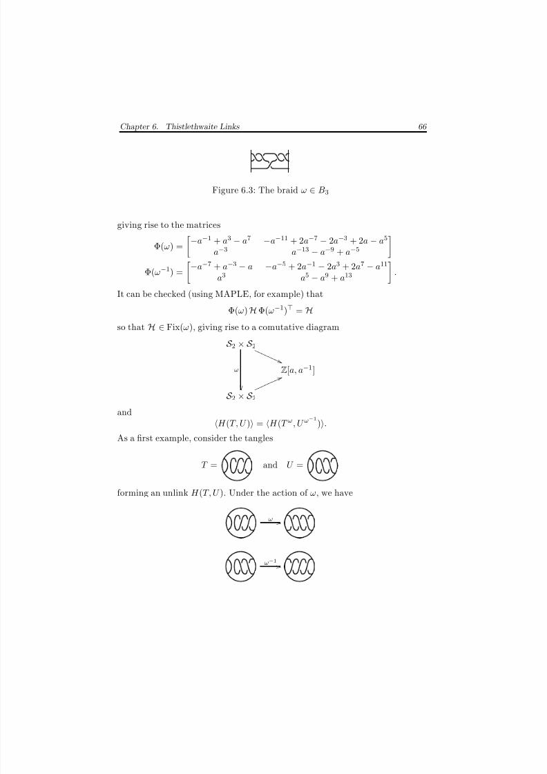
8/3/2019 Liam Thomas Watson- Knots, Tangles and Braid Actions
http://slidepdf.com/reader/full/liam-thomas-watson-knots-tangles-and-braid-actions 74/82
Chapter 6. Thistlethwaite Links 66
Figure 6.3: The braid ω ∈ B3
giving rise to the matrices
Φ(ω) = −a−1 + a3 − a7 −a−11 + 2a−7 − 2a−3 + 2a − a5
a−3
a−13
− a−9
+ a−5
Φ(ω−1) =
−a−7 + a−3 − a −a−5 + 2a−1 − 2a3 + 2a7 − a11
a3 a5 − a9 + a13
.
It can be checked (using MAPLE, for example) that
Φ(ω) H Φ(ω−1) = Hso that H ∈ Fix(ω), giving rise to a comutative diagram
S 2 × S 2
ω
( ( P P P P P P
P P
Z[a, a−1]
S 2 × S 2
6
6 n n n n n n n n
andH (T, U ) = H (T ω, U ω
−1
).
As a first example, consider the tangles
T = and U =
forming an unlink H (T, U ). Under the action of ω, we have
ω / /
ω−1 / /
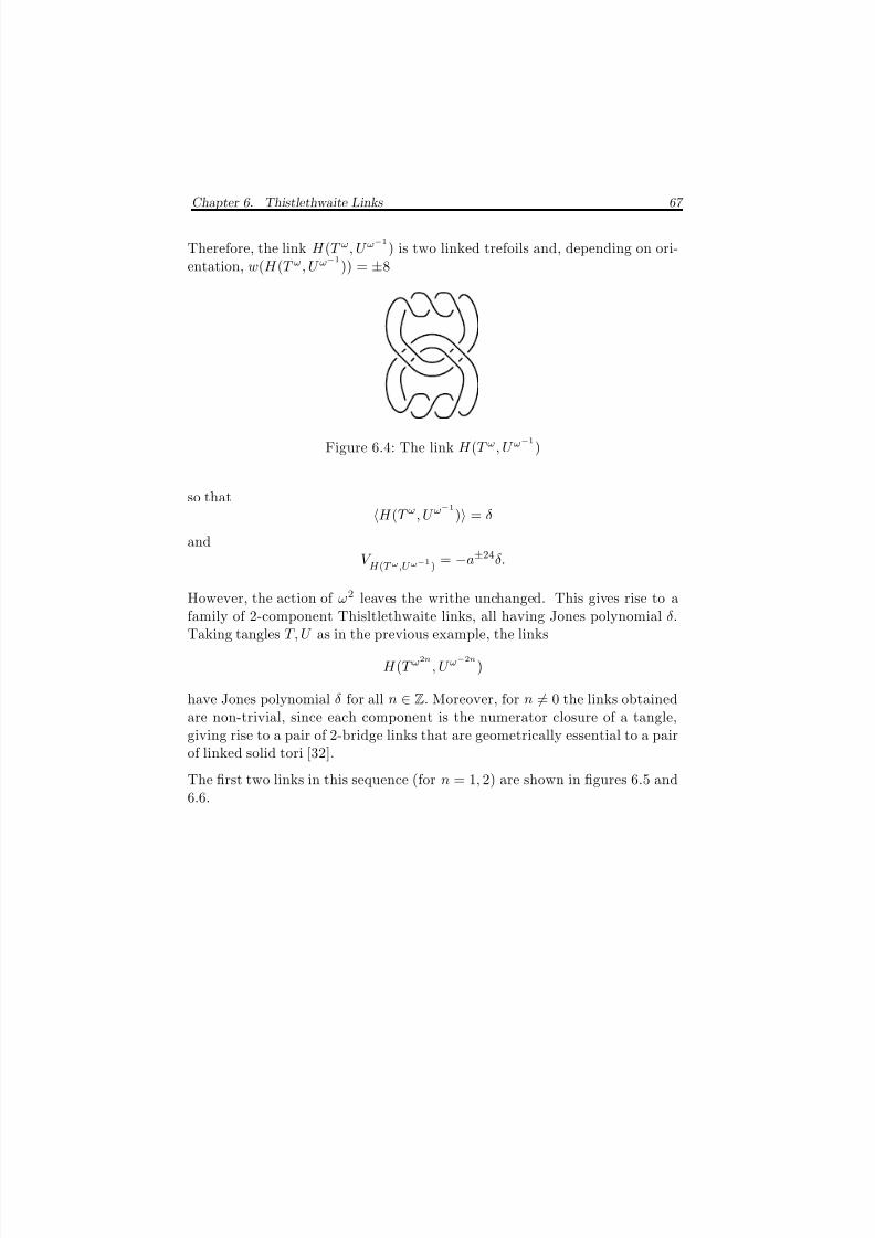
8/3/2019 Liam Thomas Watson- Knots, Tangles and Braid Actions
http://slidepdf.com/reader/full/liam-thomas-watson-knots-tangles-and-braid-actions 75/82
Chapter 6. Thistlethwaite Links 67
Therefore, the link H (T ω, U ω−1
) is two linked trefoils and, depending on ori-entation, w(H (T ω, U ω
−1
)) = ±8
Figure 6.4: The link H (T ω, U ω−1
)
so thatH (T ω, U ω
−1
) = δ
andV H (T ω,U ω−1)
= −a±24δ.
However, the action of ω2 leaves the writhe unchanged. This gives rise to afamily of 2-component Thisltlethwaite links, all having Jones polynomial δ.Taking tangles T, U as in the previous example, the links
H (T ω2n
, U ω−2n
)
have Jones polynomial δ for all n ∈ Z. Moreover, for n = 0 the links obtainedare non-trivial, since each component is the numerator closure of a tangle,giving rise to a pair of 2-bridge links that are geometrically essential to a pairof linked solid tori [32].
The first two links in this sequence (for n = 1, 2) are shown in figures 6.5 and6.6.
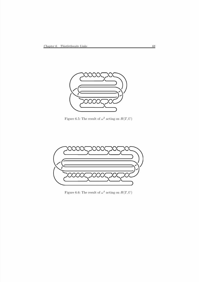
8/3/2019 Liam Thomas Watson- Knots, Tangles and Braid Actions
http://slidepdf.com/reader/full/liam-thomas-watson-knots-tangles-and-braid-actions 76/82
Chapter 6. Thistlethwaite Links 68
Figure 6.5: The result of ω2 acting on H (T, U )
Figure 6.6: The result of ω4 acting on H (T, U )
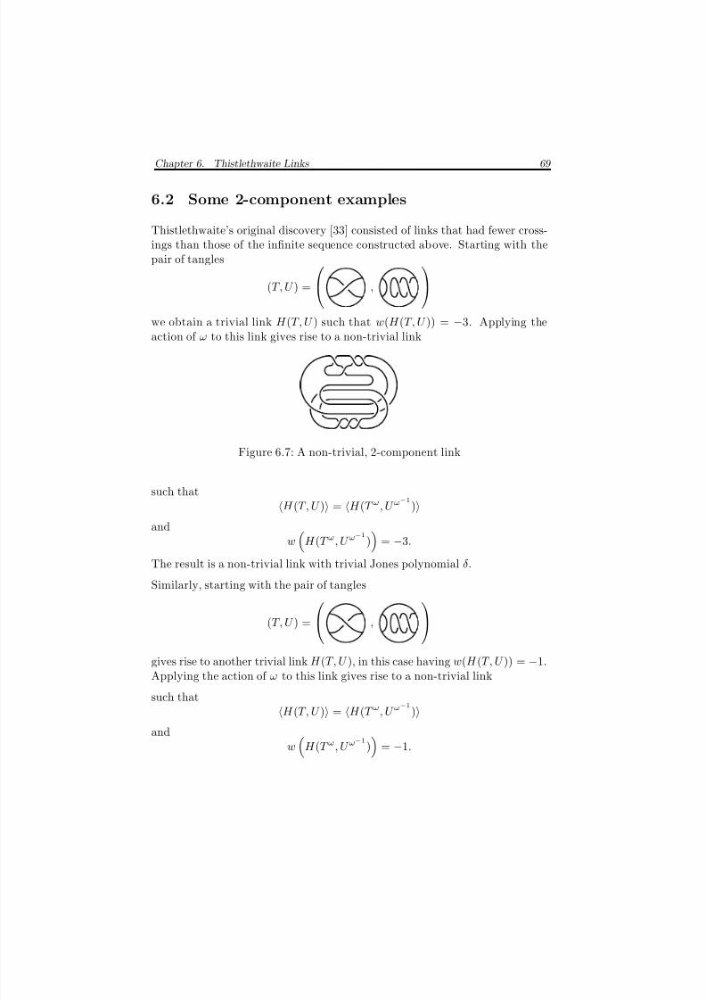
8/3/2019 Liam Thomas Watson- Knots, Tangles and Braid Actions
http://slidepdf.com/reader/full/liam-thomas-watson-knots-tangles-and-braid-actions 77/82
Chapter 6. Thistlethwaite Links 69
6.2 Some 2-component examples
Thistlethwaite’s original discovery [33] consisted of links that had fewer cross-ings than those of the infinite sequence constructed above. Starting with thepair of tangles
(T, U ) =
,
we obtain a trivial link H (T, U ) such that w(H (T, U )) = −3. Applying theaction of ω to this link gives rise to a non-trivial link
Figure 6.7: A non-trivial, 2-component link
such that H (T, U ) = H (T ω, U ω−1
)and
w
H (T ω, U ω−1
)
= −3.
The result is a non-trivial link with trivial Jones polynomial δ.
Similarly, starting with the pair of tangles
(T, U ) =
,
gives rise to another trivial link H (T, U ), in this case having w(H (T, U )) = −1.Applying the action of ω to this link gives rise to a non-trivial link
such thatH (T, U ) = H (T ω, U ω
−1
)and
w
H (T ω, U ω−1
)
= −1.
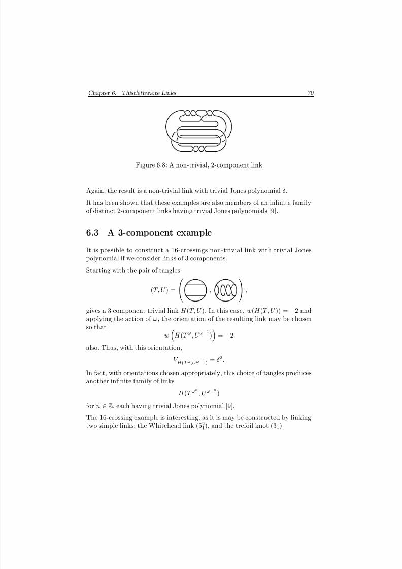
8/3/2019 Liam Thomas Watson- Knots, Tangles and Braid Actions
http://slidepdf.com/reader/full/liam-thomas-watson-knots-tangles-and-braid-actions 78/82
Chapter 6. Thistlethwaite Links 70
Figure 6.8: A non-trivial, 2-component link
Again, the result is a non-trivial link with trivial Jones polynomial δ.
It has been shown that these examples are also members of an infinite familyof distinct 2-component links having trivial Jones polynomials [9].
6.3 A 3-component example
It is possible to construct a 16-crossings non-trivial link with trivial Jonespolynomial if we consider links of 3 components.
Starting with the pair of tangles
(T, U ) = ,
,
gives a 3 component trivial link H (T, U ). In this case, w(H (T, U )) = −2 andapplying the action of ω, the orientation of the resulting link may be chosenso that
w
H (T ω, U ω−1
)
= −2
also. Thus, with this orientation,
V H (T ω ,U ω−1) = δ2.
In fact, with orientations chosen appropriately, this choice of tangles producesanother infinite family of links
H (T ωn
, U ω−n
)
for n ∈ Z, each having trivial Jones polynomial [9].
The 16-crossing example is interesting, as it is may be constructed by linkingtwo simple links: the Whitehead link (52
1), and the trefoil knot (31).
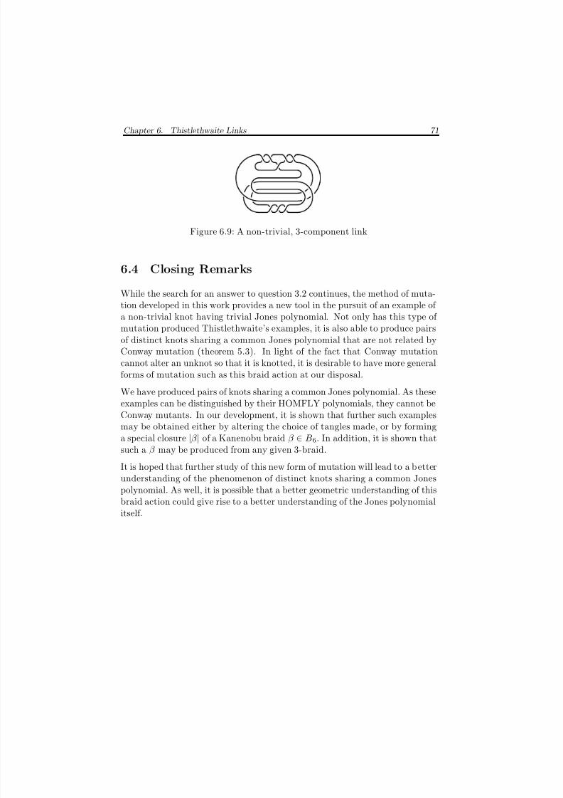
8/3/2019 Liam Thomas Watson- Knots, Tangles and Braid Actions
http://slidepdf.com/reader/full/liam-thomas-watson-knots-tangles-and-braid-actions 79/82
Chapter 6. Thistlethwaite Links 71
Figure 6.9: A non-trivial, 3-component link
6.4 Closing Remarks
While the search for an answer to question 3.2 continues, the method of muta-tion developed in this work provides a new tool in the pursuit of an example of a non-trivial knot having trivial Jones polynomial. Not only has this type of mutation produced Thistlethwaite’s examples, it is also able to produce pairsof distinct knots sharing a common Jones polynomial that are not related byConway mutation (theorem 5.3). In light of the fact that Conway mutationcannot alter an unknot so that it is knotted, it is desirable to have more generalforms of mutation such as this braid action at our disposal.
We have produced pairs of knots sharing a common Jones polynomial. As theseexamples can be distinguished by their HOMFLY polynomials, they cannot beConway mutants. In our development, it is shown that further such examplesmay be obtained either by altering the choice of tangles made, or by forminga special closure |β | of a Kanenobu braid β ∈ B6. In addition, it is shown thatsuch a β may be produced from any given 3-braid.
It is hoped that further study of this new form of mutation will lead to a b etterunderstanding of the phenomenon of distinct knots sharing a common Jonespolynomial. As well, it is possible that a better geometric understanding of thisbraid action could give rise to a better understanding of the Jones polynomialitself.
8/3/2019 Liam Thomas Watson- Knots, Tangles and Braid Actions
http://slidepdf.com/reader/full/liam-thomas-watson-knots-tangles-and-braid-actions 80/82
Bibliography
[1] J. W. Alexander. A lemma on systems of knotted curves. Proc. Nat.
Acad. Sci. USA, 9:93–95, 1923.
[2] J. W. Alexander. Topological invariants of knots and links. Trans. AMS ,
30(2):275–306, 1928.
[3] Emil Artin. Theorie der Zopfe. Abh. Math. Sem. Univ. Hamburg , 4:47–72,
1925.
[4] Emil Artin. Theory of braids. Ann. of Math., 48:101–126, 1947.
[5] Dror Bar-Natan. The knot atlas. www.math.toronto.edu/∼drorbn.
[6] Joan S. Birman. Braids, Links and Mapping Class Groups. Number 82
in Annals of Mathematics Studies. Princeton University Press, Princeton,
1974.
[7] W. Burau. Uber Zopfgruppen und gleichsinnig verdrillte Verkettunger.
Abh. Math. Sem. Hanischen Univ., 11:171–178, 1936.
[8] J. H. Conway. An enumeration of knots and links. In J. Leech, editor,
Computational problems in abstract algebra , pages 329–358. Pergamon
Press, 1970.
[9] Shalom Eliahou, Louis Kauffman, and Morwen Thistlethwaite. Infinite
families of links with trivial Jones polynomial. preprint.
[10] Roger Fenn. An elementary introduction to the theory of braids. Notes
by Bernd Gemein.
[11] Roger Fenn. Hecke algebras, 2004. Notes from ‘Knots in Vancouver’.
[12] P. Freyd, D. Yetter, J. Hoste, W. Lickorish, K. Millet, and A. Ocneanu.
A new polynomial invariant of knots and links. Bull. AMS , 12:183–312,
1985.
[13] B. Hartley and T. O. Hawkes. Rings, Modules and Linear Algebra . Chap-
man and Hall Mathematics Series. Chapman and Hall, 1971.
72
8/3/2019 Liam Thomas Watson- Knots, Tangles and Braid Actions
http://slidepdf.com/reader/full/liam-thomas-watson-knots-tangles-and-braid-actions 81/82
Bibliography 73
[14] Jim Hoste and Josef H. Przytycki. Tangle surgeries which preserve Jones-
type polynomials. Int. J. of Math., 8(8):1015–1027, 1997.
[15] Vaughan F. R. Jones. A polynomial invariant of knots via von Neumann
algebras. Bul. Amer. Math. Soc., 12:103–111, 1985.
[16] Vaughan F. R. Jones. Hecke algebra representations of braid groups and
link polynomials. Ann. of Math., 126:335–388, 1987.
[17] Taizo Kanenobu. Module d’Alexandre des noeuds fibre et polynome de
Hosokawa des lacements fibre. Math. Sem. Notes Kobe Univ., 9:75–84,
1981.
[18] Taizo Kanenobu. Infinitely many knots with the same polynomial invari-
ant. Proc. AMS , 97(1):158–162, 1986.
[19] Louis Kauffman. State models and the Jones polynomial. Topology ,
26:395–407, 1987.
[20] Louis Kauffman and Sostenes Lins. Temperley-Lieb recoupling theory and
invariants of 3-manifolds. Number 134 in Annals of Mathematics Studies.
Princeton University Press, Princeton, 1994.
[21] W. B. R. Lickorish. Three-manifolds and the Temperly-Lieb algebra.
Math. Ann., 290:657–670, 1991.
[22] W. B. R. Lickorish. Calculations with the Temperly-Lieb algebra. Com-ment. Math. Helvetici., 67:571–591, 1992.
[23] W. B. Raymond Lickorish. An Intoduction to Knot Theory . Number 175
in Graduate Texts in Mathematics. Springer, 1991.
[24] A. A. Markov. Uber die freie Aquivalenz geschlossener Zopfe. Rec. Math.Moscou , 1:73–778, 1935.
[25] John W. Milnor. Infinite cyclic coverings. In John G. Hocking, editor,
Conference on the Topology of Manifolds, volume 13 of Complementary
series in mathematics, pages 115–133. Prindle, Weber and Schmidt, 1968.
[26] H. R. Morton. Treading knot diagrams. Mth. Proc. Camb. Phil. Soc.,
99:247–260, 1986.
8/3/2019 Liam Thomas Watson- Knots, Tangles and Braid Actions
http://slidepdf.com/reader/full/liam-thomas-watson-knots-tangles-and-braid-actions 82/82
Bibliography 74
[27] Kunio Murasugi and Bohdan I. Kurpita. A Study of Braids. Mathematics
and Its Applications. Kluwer Academic Publishers, 1999.
[28] K. Reidemeister. Elementare Begrundung der Knotentheorie. Abh. Math.
Sem. Univ. Hamburg , 5:24–32, 1926.
[29] K. Reidemeister. Knotentheorie. Springer-Verlag, 1948.
[30] Dale Rolfsen. The quest for a knot with trivial Jones polynomial: Dia-
gram surgery and the Temperley-Lieb algebra. In M.E. Bozhuyuk, editor,
Topics in Knot Theory , volume 399 of Nato ASI Series C , pages 195–210.
Kluwer Academic Publishers, 1993.
[31] Dale Rolfsen. Gobal mutation of knots. J. of Knot Theory , 3(3):407–417,
1994.
[32] Dale Rolfsen. Knots and Links. AMS Chelsea, Providence, third edition,
2003.
[33] Morwen Thistlethwaite. Links with trivial Jones polynomial. preprint.
[34] Pierre Vogel. Representations of links by braids: a new algorithm. Com-
ment. Math. Helvetici , 65:104–113, 1990.


![[CLICK TO ENLARGE] Tangles Newsletter: SUMMER EDITION](https://img.pdfslide.us/doc/110x75/568c547c1a28ab4916beff06/click-to-enlarge-tangles-newsletter-summer-edition.jpg)


![[CLICK TO ENLARGE] Tangles Newsletter: AUTUMN EDITION](https://img.pdfslide.us/doc/110x75/568c57641a28ab4916ca5269/click-to-enlarge-tangles-newsletter-autumn-edition-5704042245d70.jpg)