Leverage Restrictions in a Business Cycle Model ∗

Lawrence Christiano†and Daisuke Ikeda‡

January 9, 2013

Abstract

We modify an otherwise standard medium-sized DSGE model, in order to study the

macroeconomic effects of placing leverage restrictions on financial intermediaries. The

financial intermediaries (‘bankers’) in the model must exert effort in order to earn high

returns for their creditors. An agency problem arises because banker effort is not observ-

able to creditors. The consequence of this agency problem is that leverage restrictions on

banks generate a very substantial welfare gain in steady state. We discuss the economics

of this gain. As a way of testing the model, we explore its implications for the dynamic

effects of shocks.

∗We are grateful for advice from Yuta Takahashi and to Thiago Teixeira Ferreira for kindly allowing us touse the cross-sectional dispersion data he constructed and which is reported in Figure 1. We are particularlygrateful to Saki Bigio, for his very insightful discussion (Bigio, 2012a) at the conference for which this paperwas prepared. We also benefitted from the observations of the other conference participants, especially TobiasAdrian, John Geanakoplos and Robert Hall. The manuscript was prepared for the XVI Annual Conferenceof the Central Bank of Chile, “Macroeconomics and Financial Stability: Challenges for Monetary Policy,”November 15-16, 2012.†Northwestern University and National Bureau of Economic Research, e-mail: l-christiano@nothwestern.edu‡Bank of Japan, E-mail: daisuke.ikeda@boj.or.jp. The views expressed in the paper are those of the authors

and should not be interpreted as the offi cial views of the Bank of Japan.

1 Introduction

We seek to develop a business cycle model with a financial sector, which can be used to study

the consequences of policies to restrict the leverage of financial institutions (‘banks’).1 Because

we wish the model to be consistent with basic features of business cycle data, we introduce our

banking system into a standard medium sized DSGE model such as Christiano, Eichenbaum

and Evans (2005) (CEE) or Smets andWouters (2007). Banks in our model operate in perfectly

competitive markets. Our model implies that social welfare is increased by restricting bank

leverage relative to what leverage would be if financial markets were unregulated. With less

leverage, banks are better able to use their net worth to insulate creditors in case there are

losses on bank balance sheets. Our model implies that by reducing risk to creditors, agency

problems are mitigated and the effi ciency of the banking system is improved. We explore the

economics of our result by studying the model’s steady state. We also display various dynamic

features of the model to assess its empirical plausibility.

There are two types of motivations for restrictions on banking leverage. One motivates

leverage restrictions as a device to correct an agency problem in the private economy. Another

motivates leverage restrictions as a device to correct a commitment problem in the government.2

In this paper we focus on the former type of rationale for leverage restrictions.

We posit the existence of an agency problem between banks and their creditors. By bank

creditors we have in mind real-world depositors, holders of debt securities like bonds and

commercial paper, and also holders of bank preferred stock.3 As a result, bank credit in our

1By ‘banks’we mean all financial institutions, not just commercial banks.2For example, Chari and Kehoe (2012) show that a case for leverage restrictions can be built on the

assumptions that (i) bankruptices are ex post ineffi cient and (ii) governments are unable to commit ex anteto not bailout failed banks. See also Gertler, Kiyotaki and Queralto (2011) for a discussion. In the generaldiscussion of Adrian, Colla and Shin (forthcoming), Robert Hall draws attention to the implications for bankleverage decisions of the expectation of government intervention in a crisis episode.

3Our logic for including bank preferred stock in bank ‘credit’is as follows. In our model, the liability side ofbank balance sheets has only ‘bank debt’and ‘bank net worth’. For the vast majority of banks in our model,their asset portfolio performs well enough that debt holders receive a high return and bank net worth generallyearns a positive return. In the case of banks in our model whose portfolio of assets performs poorly, net worthis wiped out and debt holders earn a low return. The reason we think of preferred stock as part of bank debt inthe model is: (i) dividend payments on preferred stock are generally not contingent on the overall performanceof the bank’s assets, unless the performance of the assets is so bad that common stock holders are wipedout; and (ii) like ordinary debt, holders of preferred stock do not enjoy voting rights. Our model abstractsfrom the differences that do exist between the different components of what we call bank debt. For example,dividends on preferred stock are paid after interest and principal payments on a bank’s bonds, commercialpaper and deposits. In addition, the tax treatment of preferred stock is different from the tax treatment ofa bank’s bond and commercial paper. The reason we identify the common stock portion of bank liabilitieswith bank net worth in our model is that holders of common stock are residual claimants. As a result, theyare the recipients of increases in bank earnings (magnified by leverage) and they suffer losses when earningsare low (and, these losses are magnified by leverage). Financial firms are very important in the market forpreferred stock. For example, Standard and Poor’s computes an overall index of the price and yield on preferredstock. In their index for December 30, 2011, 82 percent of the firms belong to the financial sector (see https://www.sp-indexdata.com/idpfiles/strategy/prc/active/factsheets/fs-sp-us-preferred-stock-index-ltr.pdf).

1

model is risky. To quantify this risk, we calibrate the model to the premium paid by banks

for funds in the interbank market. This premium is on average about 50 basis points at an

annual rate.4 To simplify the analysis, we assume there is no agency problem on the asset side

of banks’balance sheets. The role of banks in our model is to exert costly effort to identify

good investment projects. The source of the agency problem in our model is our assumption

that bank effort is not observed. Under these circumstances it is well known that competitive

markets do not necessarily generate the effi cient allocations. In our analysis, the fact that

banker effort is unobserved has the consequence that restricting the amount of liabilities a

bank may issue raises welfare.

As in any model with hidden effort, the resulting agency problem is mitigated if the market

provides the agent (i.e., the banker) with the appropriate incentives to exert effort. For this,

it is useful if the interest rate that the banker pays to its creditors is not sensitive to the

performance of the asset side of its balance sheet. In this case, the banker reaps the full reward

of its effort. But, this requires that the banker have suffi cient net worth on hand to cover the

losses that will occasionally occur even if a high level of effort is expended. The creditors in

low net worth banks which experience bad outcomes on their portfolio necessarily must share

in bank losses. Understanding this in advance, creditors require that low net worth bankers

with well-performing porfolios pay a high interest rate. Under these circumstances, the banker

does not enjoy the full fruits of its effort and so its incentive to exert effort is correspondingly

reduced.

We analyze the steady state properties of the model and show that a leverage restriction

moves equilibrium consumption and employment in the direction of the effi cient allocations

that would occur if effort were observable. In particular, when banks are restricted in how

many liabilities they can issue, then they are more likely to be able to insulate their creditors

from losses on the asset side of their balance sheet. In this way leverage restrictions reduce the

interest rate spread faced by banks and promote their incentive to exert effort. We calibrate

our model’s parameters so that leverage is 20 in the absence of regulation. When a regulation

is imposed that limits leverage to 17, steady state welfare jumps an amount that is equivalent

to a permanent 1.19 percent jump in consumption.5

After obtaining these results for the steady state of the model, we turn to its dynamic

4We measure the interest rate on the interbank market by the 3 month London interbank offer rate (LIBOR).The interest rate premium is the excess of LIBOR over the 3 month rate on US government Treasury bills.

5In our analysis, we do not factor in the bureaucratic and other reporting costs of leverage restrictions. If wedo so, presumably the steady state welfare benefit of leverage would be smaller. However, because the benefitsreported in this paper are so large, we expect our finding that welfare increases to be robust.

2

properties. We display the dynamic response of various variables to four shocks. Of these,

one is a monetary policy shock, two are shocks to bank net worth and fourth is a shock

to the cross-sectional dispersion of technology.6 In each case, a contractionary shock drives

down consumption, investment, output, employment, inflation and bank net worth, just as

in actual recessions. In addition, all four shocks raise the cross-sectional dispersion of bank

equity returns. We use Center for Research on Security Prices (CRSP) data to show that

this implication is consistent with the data. The countercyclical nature of various measures

of dispersion has been a subject of great interest since Bloom (2009) drew attention to the

phenomenon. A factor that may be of independent interest is that our paper provides examples

of how this increase in dispersion can occur endogenously. Finally, we show that the shocks in

our model imply that bank leverage is countercyclical. We show that broad-based empirical

measures of leverage are consistent with this implication.

The paper is organized as follows. The next section describes the circumstances of the

bankers. We then describe the general macroeconomic environment into which we insert the

bank. After that we report our findings for leverage and for the dynamic properties of our

model. A last section includes concluding remarks.

2 Banks, Mutual Funds and Entrepreneurs

We begin the discussion in period t, after goods production for that period has occurred.

There is a mass of identical bankers with net worth, Nt. The bankers enter into competitive

and anonymous markets, acquire deposits from mutual funds and lend their net worth and

deposits to entrepreneurs. Mutual funds take deposits from households and make loans to

a diversified set of banks. The assumption that mutual funds stand between households and

banks is made for convenience. Our bankers are risky and if households placed deposits directly

with banks they would choose to diversify across banks. The idea that households diversify

across a large set of banks seemed awkward to us. Instead, we posit that households place their

deposits with mutual funds, and then mutual funds diversify across banks. Another advantage

of our assumption that mutual funds stand between households and banks is that this allows

us to define a risk free rate of interest. However, nothing of substance hinges on the presence

of the mutual funds.

Each entrepreneur has access to a constant returns to scale investment technology. The

technology requires as input an investment at the end of goods production in period t and

6For the latter we consider a risk shock, as in Christiano, Motto and Rostagno (2012).

3

produces output during production in t + 1. Entrepreneurs are competitive, earn no rent

and there is no agency problem between entrepreneurs and banks. The bank from which an

entrepreneur receives its loan receives the full rate of return earned by entrepreneurs on their

projects.

There are ‘good’ and ‘bad’ entrepreneurs. We denote the gross rate of return on their

period t investment by Rgt+1 and R

bt+1, respectively, where R

gt+1 > Rb

t+1 in all period t + 1

states of nature. These represent exogenous stochastic processes from the point of view of

entrepreneurs. We discuss the factors that determine these rates of return in the next section.

There, we situate entrepreneurs and bankers in the broader macro economy.

A key function of banks is to identify good entrepreneurs. To do this, bankers exert a costly

effort. In our baseline model this effort is not observable to the mutual funds that supply the

banks with funds, and this creates an agency problem on the liability side of a bank’s balance

sheet. As a convenient benchmark, we also consider the version of the model in which banker

effort is observable to the mutual fund which supplies the bank with deposits, dt.

At the end of production in period t each banker takes deposits, dt and make loans in

the amount, Nt + dt, to entrepreneurs. We capture the idea that banks are risky with the

assumption that a bank can only invest in one entrepreneur.7 The quantities, Nt and dt are

expressed in per capita terms.

We denote the effort exerted by a banker to find a good entrepreneur by et. The banker iden-

tifies a good entrepreneur with probability pt (et) and a bad entrepreneur with the complemen-

tary probability. For computational simplicity, we adopt the following simple representation

of the probability function:

p (e) = min{

1, a+ be}, a, b ≥ 0

Because we work with equilibria in which p (e) > 1/2, our model implies that when bankers

exert greater effort, the mean return on their asset increases and its variance decreases.

Mutual funds are competitive and perfectly diversified across good and bad banks. As a

result of free entry, they enjoy zero profits:

p (et)Rdg,t+1 + (1− p (et))R

db,t+1 = Rt, (1)

7We can describe the relationship between a bank and an entrepreneur in search theoretic terms. Thus,the bank exerts an effort, et, to find an entrepreneur. Upon exerting this effort a bank meets exactly oneentrepreneur in a period. We imagine that the outside option for both the banker and the entrepreneur at thispoint is zero. We suppose that upon meeting, the bank has the option to make a take-it-or-leave-it offer to theentrepreneur. Under these circumstances, the bank will make an offer that puts the entrepreneur on its outsideoption of zero. In this way, the banker captures all the rent in their relationship.

4

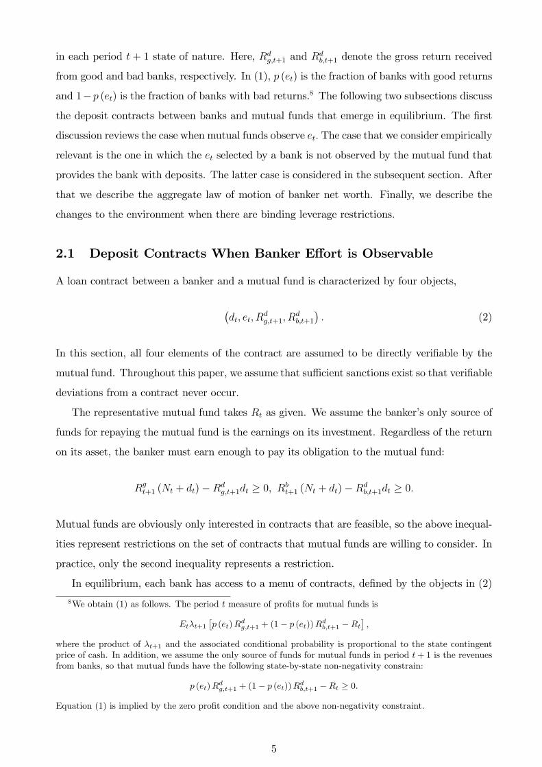
in each period t + 1 state of nature. Here, Rdg,t+1 and R

db,t+1 denote the gross return received

from good and bad banks, respectively. In (1), p (et) is the fraction of banks with good returns

and 1− p (et) is the fraction of banks with bad returns.8 The following two subsections discuss

the deposit contracts between banks and mutual funds that emerge in equilibrium. The first

discussion reviews the case when mutual funds observe et. The case that we consider empirically

relevant is the one in which the et selected by a bank is not observed by the mutual fund that

provides the bank with deposits. The latter case is considered in the subsequent section. After

that we describe the aggregate law of motion of banker net worth. Finally, we describe the

changes to the environment when there are binding leverage restrictions.

2.1 Deposit Contracts When Banker Effort is Observable

A loan contract between a banker and a mutual fund is characterized by four objects,

(dt, et, R

dg,t+1, R

db,t+1

). (2)

In this section, all four elements of the contract are assumed to be directly verifiable by the

mutual fund. Throughout this paper, we assume that suffi cient sanctions exist so that verifiable

deviations from a contract never occur.

The representative mutual fund takes Rt as given. We assume the banker’s only source of

funds for repaying the mutual fund is the earnings on its investment. Regardless of the return

on its asset, the banker must earn enough to pay its obligation to the mutual fund:

Rgt+1 (Nt + dt)−Rd

g,t+1dt ≥ 0, Rbt+1 (Nt + dt)−Rd

b,t+1dt ≥ 0.

Mutual funds are obviously only interested in contracts that are feasible, so the above inequal-

ities represent restrictions on the set of contracts that mutual funds are willing to consider. In

practice, only the second inequality represents a restriction.

In equilibrium, each bank has access to a menu of contracts, defined by the objects in (2)

8We obtain (1) as follows. The period t measure of profits for mutual funds is

Etλt+1[p (et)R

dg,t+1 + (1− p (et))R

db,t+1 −Rt

],

where the product of λt+1 and the associated conditional probability is proportional to the state contingentprice of cash. In addition, we assume the only source of funds for mutual funds in period t+ 1 is the revenuesfrom banks, so that mutual funds have the following state-by-state non-negativity constrain:

p (et)Rdg,t+1 + (1− p (et))R

db,t+1 −Rt ≥ 0.

Equation (1) is implied by the zero profit condition and the above non-negativity constraint.

5

which satisfy (1) and

Rbt+1 (Nt + dt)−Rd

b,t+1dt ≥ 0, (3)

as well as non-negativity of et and dt. The problem of the banker is to select a contract from

this menu.

A banker’s ex ante reward from a loan contract is:

Etλt+1

{p (et)

[Rgt+1 (Nt + dt)−Rd

g,t+1dt]

+ (1− p (et))[Rbt+1 (Nt + dt)−Rd

b,t+1dt]}− 1

2e2t , (4)

where e2t/2 is the banker’s utility cost of expending effort and λt+1 denotes the marginal value

of profits to the household. As part of the terms of the banker’s arrangement with its own

household, the banker is required to seek a contract that maximizes (4).9 Formally, the banker

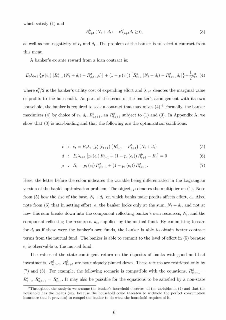
maximizes (4) by choice of et, dt, Rdg,t+1, an R

db,t+1 subject to (1) and (3). In Appendix A, we

show that (3) is non-binding and that the following are the optimization conditions:

e : et = Etλt+1p′t (et+1)

(Rgt+1 −Rb

t+1

)(Nt + dt) (5)

d : Etλt+1

[pt (et)R

gt+1 + (1− pt (et))R

bt+1 −Rt

]= 0 (6)

µ : Rt = pt (et)Rdg,t+1 + (1− pt (et))R

db,t+1. (7)

Here, the letter before the colon indicates the variable being differentiated in the Lagrangian

version of the bank’s optimization problem. The object, µ denotes the multiplier on (1). Note

from (5) how the size of the base, Nt + dt, on which banks make profits affects effort, et. Also,

note from (5) that in setting effort, e, the banker looks only at the sum, Nt + dt, and not at

how this sum breaks down into the component reflecting banker’s own resources, Nt, and the

component reflecting the resources, dt, supplied by the mutual fund. By committing to care

for dt as if these were the banker’s own funds, the banker is able to obtain better contract

terms from the mutual fund. The banker is able to commit to the level of effort in (5) because

et is observable to the mutual fund.

The values of the state contingent return on the deposits of banks with good and bad

investments, Rdg,t+1, R

db,t+1 are not uniquely pinned down. These returns are restricted only by

(7) and (3). For example, the following scenario is compatible with the equations, Rdg,t+1 =

Rgt+1, R

db,t+1 = Rb

t+1. It may also be possible for the equations to be satisfied by a non-state

9Throughout the analysis we assume the banker’s household observes all the variables in (4) and that thehousehold has the means (say, because the household could threaten to withhold the perfect consumptioninsurance that it provides) to compel the banker to do what the household requires of it.

6

contingent pattern of returns, Rdg,t+1 = Rd

b,t+1 = Rt. However, (3) indicates that the latter case

requires Nt to be suffi ciently large.

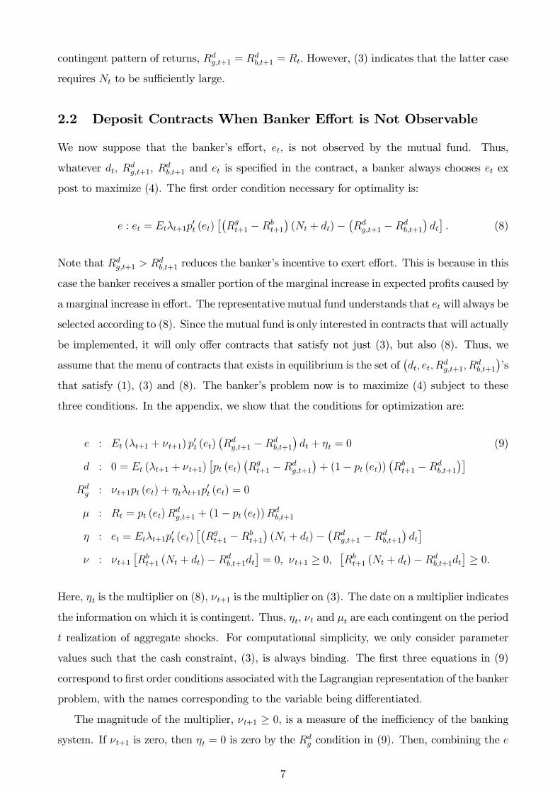
2.2 Deposit Contracts When Banker Effort is Not Observable

We now suppose that the banker’s effort, et, is not observed by the mutual fund. Thus,

whatever dt, Rdg,t+1, R

db,t+1 and et is specified in the contract, a banker always chooses et ex

post to maximize (4). The first order condition necessary for optimality is:

e : et = Etλt+1p′t (et)

[(Rgt+1 −Rb

t+1

)(Nt + dt)−

(Rdg,t+1 −Rd

b,t+1

)dt]. (8)

Note that Rdg,t+1 > Rd

b,t+1 reduces the banker’s incentive to exert effort. This is because in this

case the banker receives a smaller portion of the marginal increase in expected profits caused by

a marginal increase in effort. The representative mutual fund understands that et will always be

selected according to (8). Since the mutual fund is only interested in contracts that will actually

be implemented, it will only offer contracts that satisfy not just (3), but also (8). Thus, we

assume that the menu of contracts that exists in equilibrium is the set of(dt, et, R

dg,t+1, R

db,t+1

)’s

that satisfy (1), (3) and (8). The banker’s problem now is to maximize (4) subject to these

three conditions. In the appendix, we show that the conditions for optimization are:

e : Et (λt+1 + νt+1) p′t (et)(Rdg,t+1 −Rd

b,t+1

)dt + ηt = 0 (9)

d : 0 = Et (λt+1 + νt+1)[pt (et)

(Rgt+1 −Rd

g,t+1

)+ (1− pt (et))

(Rbt+1 −Rd

b,t+1

)]Rdg : νt+1pt (et) + ηtλt+1p

′t (et) = 0

µ : Rt = pt (et)Rdg,t+1 + (1− pt (et))R

db,t+1

η : et = Etλt+1p′t (et)

[(Rgt+1 −Rb

t+1

)(Nt + dt)−

(Rdg,t+1 −Rd

b,t+1

)dt]

ν : νt+1

[Rbt+1 (Nt + dt)−Rd

b,t+1dt]

= 0, νt+1 ≥ 0,[Rbt+1 (Nt + dt)−Rd

b,t+1dt]≥ 0.

Here, ηt is the multiplier on (8), νt+1 is the multiplier on (3). The date on a multiplier indicates

the information on which it is contingent. Thus, ηt, νt and µt are each contingent on the period

t realization of aggregate shocks. For computational simplicity, we only consider parameter

values such that the cash constraint, (3), is always binding. The first three equations in (9)

correspond to first order conditions associated with the Lagrangian representation of the banker

problem, with the names corresponding to the variable being differentiated.

The magnitude of the multiplier, νt+1 ≥ 0, is a measure of the ineffi ciency of the banking

system. If νt+1 is zero, then ηt = 0 is zero by the Rdg condition in (9). Then, combining the e

7

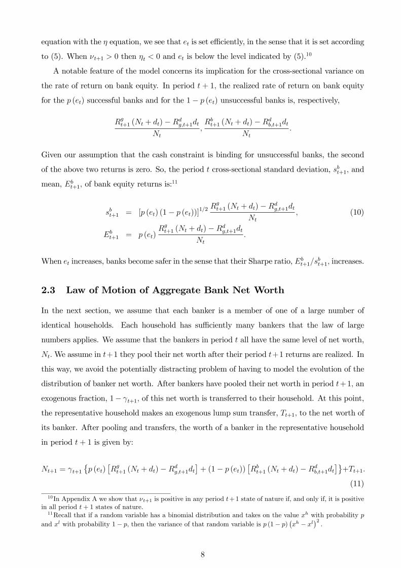
equation with the η equation, we see that et is set effi ciently, in the sense that it is set according

to (5). When νt+1 > 0 then ηt < 0 and et is below the level indicated by (5).10

A notable feature of the model concerns its implication for the cross-sectional variance on

the rate of return on bank equity. In period t + 1, the realized rate of return on bank equity

for the p (et) successful banks and for the 1− p (et) unsuccessful banks is, respectively,

Rgt+1 (Nt + dt)−Rd

g,t+1dt

Nt

,Rbt+1 (Nt + dt)−Rd

b,t+1dt

Nt

.

Given our assumption that the cash constraint is binding for unsuccessful banks, the second

of the above two returns is zero. So, the period t cross-sectional standard deviation, sbt+1, and

mean, Ebt+1, of bank equity returns is:

11

sbt+1 = [p (et) (1− p (et))]1/2 R

gt+1 (Nt + dt)−Rd

g,t+1dt

Nt

, (10)

Ebt+1 = p (et)

Rgt+1 (Nt + dt)−Rd

g,t+1dt

Nt

.

When et increases, banks become safer in the sense that their Sharpe ratio, Ebt+1/s

bt+1, increases.

2.3 Law of Motion of Aggregate Bank Net Worth

In the next section, we assume that each banker is a member of one of a large number of

identical households. Each household has suffi ciently many bankers that the law of large

numbers applies. We assume that the bankers in period t all have the same level of net worth,

Nt.We assume in t+1 they pool their net worth after their period t+1 returns are realized. In

this way, we avoid the potentially distracting problem of having to model the evolution of the

distribution of banker net worth. After bankers have pooled their net worth in period t+ 1, an

exogenous fraction, 1− γt+1, of this net worth is transferred to their household. At this point,

the representative household makes an exogenous lump sum transfer, Tt+1, to the net worth of

its banker. After pooling and transfers, the worth of a banker in the representative household

in period t+ 1 is given by:

Nt+1 = γt+1

{p (et)

[Rgt+1 (Nt + dt)−Rd

g,t+1dt]

+ (1− p (et))[Rbt+1 (Nt + dt)−Rd

b,t+1dt]}

+Tt+1.

(11)

10In Appendix A we show that νt+1 is positive in any period t+ 1 state of nature if, and only if, it is positivein all period t+ 1 states of nature.11Recall that if a random variable has a binomial distribution and takes on the value xh with probability p

and xl with probability 1− p, then the variance of that random variable is p (1− p)(xh − xl

)2.

8

We assume that γt+1 and Tt+1 are exogenous shocks, realized in t+1. A rise in Tt+1 is equivalent

to an influx of new equity into the banks. Similarly, a rise in γt+1 also represents a rise in

equity. Thus, we assume that the inflow or outflow of equity into the banks is exogenous and

is not subject to the control of the banker. The only control bankers have over their net worth

operates through their contol over deposits and the resulting impact on their earnings.

In the unobserved effort model, where we assume the cash constraint is always binding in

the bad state, we have:

Nt+1 = γt+1p (et)[Rgt+1 (Nt + dt)−Rd

g,t+1dt]

+ Tt+1. (12)

The object in square brackets is the realized profits of good banks. It is possible for those to

make losses on their deposits (i.e., Rgt+1 < Rd

g,t+1), however we assume that those profits are

never so negative that they cannot be covered by earnings on net worth.

When there is no aggregate uncertainty, the d and µ equations (9) imply that the expected

earnings of a bank on deposits is zero. Then,

pt (et)Rgt+1 + (1− pt (et))R

bt+1 = Rt. (13)

Equation (13) and the µ equation in (9) together imply that the law of motion has the following

form:

Nt+1 = γt+1RtNt + Tt+1. (14)

When there is aggregate uncertainty, equation (13) holds only in expectation. It does not hold

in terms of realized values.

2.4 Restrictions on Bank Leverage

We now impose an additional constraint on banks, that they must satisfy:

Nt + dtNt

≤ Lt, (15)

where Lt denotes the period t restriction on leverage. The banker problem now is (A.3) with

the additional constraint, NtLt − (Nt + dt) ≥ 0. Let Λt ≥ 0 denote the multiplier on that

constraint. It is easy to verify that the equilibrium conditions now are (9) with the zero in the

d equation replaced by Λt, plus the following complementary slackness condition:

Λt [NtLt − (Nt + dt)] = 0, Λt ≥ 0, NtLt − (Nt + dt) ≥ 0.

9

Thus, when the leverage constraint is binding, we use the d equation to define Λt and add the

equation

NtLt = (Nt + dt) .

Interestingly, since the d equation does not hold any longer with Λt = 0, the expected

profits of banks in steady state are positive. As a result, (14) does not hold in steady state.

Of course, (11) and (12) both hold. Using the µ equation to simplify (11):

Nt+1 = γt+1

{[pt (et)R

gt+1 + (1− pt (et))R

bt+1

](Nt + dt)−Rtdt

}+ Tt+1. (16)

The modified d equation in the version of the model without aggregate uncertainty is:

Λt = (λt+1 + νt+1)[pt (et)

(Rgt+1 −Rd

g,t+1

)+ (1− pt (et))

(Rbt+1 −Rd

b,t+1

)]. (17)

Substituting this into (16):

Nt+1 = γt+1

{[Λt

λt+1 + νt+1

+Rt

](Nt + dt)−Rtdt

}+ Tt+1,

or

Nt+1 = γt+1

{RtNt +

[Λt

λt+1 + νt+1

](Nt + dt)

}+ Tt+1.

From here we see that banks make profits on deposits when the leverage constraint is binding,

so that Λt > 0.

3 The General Macroeconomic Environment

In this section, we place the financial markets of the previous section into an otherwise stan-

dard macro model, along the lines of Christiano, Eichenbaum and Evans (2005) or Smets and

Wouters (2007). The financial market has two points of contact with the broader macroeco-

nomic environment. First, the rates of return on entrepreneurial projects are a function of

the rate of return on capital. Second, there is a market clearing condition in which the total

purchases of raw capital by entrepreneurs, Nt + dt, is equal to the total supply of raw capital

by capital producers. In the following two subsections, we first describe goods production and

the problem of households. The second subsection describes the production of capital and its

links to the entrepreneur. Later subsections describe monetary policy and other aspects of the

macro model.

10

3.1 Goods Production

Goods are produced according to a Dixit-Stiglitz structure. A representative, competitive final

goods producer combines intermediate goods, Yjt, j ∈ [0, 1], to produce a homogeneous good,

Yt, using the following technology:

Yt =

[∫ 1

0

Yj,t1λf dj

]λf, 1 ≤ λf <∞. (18)

The intermediate good is produced by a monopolist using the following technology:

Yj,t =

Kαj,t (ztljt)

1−α − Φz∗t if Kαj,t (ztlj,t)

1−α > Φz∗t

0 otherwise, 0 < α < 1. (19)

Here, zt follows a determinist time trend. Also, Kj,t denotes the services of capital and lj,t

denotes the quantity of homogeneous labor, respectively, hired by the jth intermediate good

producer. The fixed cost in the production function, (19), is proportional to z∗t , which is

discussed below. The variable, z∗t , has the property that Yt/z∗t converges to a constant in

non-stochastic steady state. The monopoly supplier of Yj,t sets its price, Pj,t, subject to Calvo-

style frictions. Thus, in each period t a randomly-selected fraction of intermediate-goods firms,

1− ξp, can reoptimize their price. The complementary fraction sets its price as follows:

Pj,t = πPj,t−1.

Let πt denote the gross rate of inflation, Pt/Pt−1, where Pt is the price of Yt. Then, π denotes

the steady state value of inflation.

There exists a technology that can be used to convert homogeneous goods into consumption

goods, Ct, one-for-one. Another technology converts a unit of homogenous goods into Υt

investment goods, where Υ > 1. This parameter allows the model to capture the observed

trend fall in the relative price of investment goods. Because we assume these technologies are

operated by competitive firms, the equilibrium prices of consumption and investment goods

are Pt and

PI,t =PtΥt,

respectively. The trend rise in technology for producing investment goods is the second source

of growth in the model, and

z∗t = ztΥ( α1−α)t.

11

Our treatment of the labor market follows Erceg, Henderson and Levin (2000), and parallels

the Dixit-Stiglitz structure of goods production. A representative, competitive labor contractor

aggregates the differentiated labor services, hi,t, i ∈ [0, 1] , into homogeneous labor, lt, using

the following production function:

lt =

[∫ 1

0

(hi,t)1λw di

]λw, 1 ≤ λw. (20)

The labor contractor sells labor services, lt, to intermediate good producers for a given nominal

wage rate,Wt. The labor contractor also takes as given the wages of the individual labor types,

Wi,t.

A representative, identical household supplies each of the differentiated labor types, hi,t, i ∈

[0, 1] , used by the labor contractors. By assuming that all varieties of labor are contained within

the same household (this is the ‘large family’assumption introduced by Andolfatto (1996) and

Merz (1995)) we avoid confronting diffi cult - and potentially distracting - distributional issues.

For each labor type, i ∈ [0, 1] , there is a monopoly union that represents workers of that type

belonging to all households. The ith monopoly union sets the wage rate, Wit, for its members,

subject to Calvo-style frictions. In particular, a randomly selected subset of 1− ξw monopoly

unions set their wage to optimize household utility (see below), while the complementary subset

sets the wage according to:

Wi,t = µz∗πWi,t−1.

Here, µz∗ denotes the growth rate of z∗t . The wage rate determines the quantity of labor

demanded by the competitive labor aggregators. Households passively supply the quantity of

labor demanded.

3.2 Households

The representative household is composed of a unit measure of agents. Of these, a fraction %

are workers and the complementary fraction are bankers. Per capita household consumption

is Ct, which is distributed equally to all household members. Average period utility across all

workers is given by:

log(Ct − buCt−1)− ψL∫ 1

0

h1+σLi,t

1 + σLdi, ψL, σL ≥ 0.

12

The object, bu ≥ 0, denotes the parameter controlling the degree of habit persistence. The

period utility function of a banker is:

log(Ct − buCt−1)− %e2t , % ≡

1

2 (1− %). (21)

The representative household’s utility function is the equally-weighted average across the utility

of all the workers and bankers:

log(Ct − buCt−1)− ψL∫ 1

0

h1+σLi,t

1 + σLdi− 1

2e2t , ψL ≡ %ψL.

The representative household’s discount value of a stream of consumption, employment and

effort is valued as follows:

E0

∞∑t=0

βt

{log(Ct − buCt−1)− ψL

∫ 1

0

h1+σLi,t

1 + σLdi− 1

2e2t

}, ψL, bu, σL > 0. (22)

Bankers behave as described in section 2. They are assumed to do so in exchange for the

perfect consumption insurance received from households. Although the mutual funds from

which bankers obtain deposits do not observe banker effort, et, we assume that a banker’s own

household observes everything that it does. By instructing the bankers to maximize expected

net worth (taking into account their own costs of exerting effort), the household maximizes

total end-of-period banker net worth.12

The representative household takes et and labor earnings as given. It chooses Ct and the

quantity of a nominal bond, Bt+1, to maximize (22) subject to the budget constraint:

PtCt +Bt+1 ≤∫ 1

0

Wi,thi,tdi+RtBt + Πt.

Here, Πt denotes lump sum transfers of profits from intermediate good firms and bankers and

taxes. In addition, the household has access to a nominally non-state contingent one-period

12

A brief observation about units of measure. We measure the financial objects that the banker works with,Nt and dt in per capita terms. Bankers are a fraction, 1 − %, of the population, so that in per banker terms,bankers work with Nt/ (1− %) and dt/ (1− %) . We assume the banker values profits net of the utility cost ofits effort as follows:

Etλt+1

{p (et)

[Rgt+1

(Nt + dt1− %

)−Rdg,t+1

dt1− %

]+ (1− p (et))

[Rbt+1

(Nt + dt1− %

)−Rdb,t+1

dt1− %

]}− %e2t .

Multiplying this expression by 1− % and using (21), we obtain (4).

13

bond with gross payoffRt in period t+ 1. Loan market clearing requires that, in equilibrium:

Bt = dt. (23)

3.3 Monetary Policy

We express the monetary authority’s policy rule directly in linearized form:

Rt −R = ρp (Rt−1 −R) +(1− ρp

) [απ (πt+1 − π) + α∆y

1

4(gy,t − µz∗)

]+

1

400εpt , (24)

where εpt is a shock to monetary policy and ρp is a smoothing parameter in the policy rule.

Here, Rt − R is the deviation of the period t net quarterly interest rate, Rt, from its steady

state. Similarly, πt+1 − π is the deviation of anticipated quarterly inflation from the central

bank’s inflation target. The expression, gy,t − µz∗ is quarterly GDP growth, in deviation from

its steady state. Finally, εpt is an iid shock to monetary policy with standard deviation, σp.

Note that the shock is in units of annual percentage points.

3.4 Capital Producers, Entrepreneurial Returns and Market Clear-

ing Conditions

In this section we explain how entrepreneurial returns are linked to the underlying return on

physical capital. In addition, we discuss the agents that produce capital, the capital producers.

Finally, we present the final goods market clearing condition and the market clearing for capital.

The sole source of funds available to an entrepreneur is the funds, Nt + dt, received from

its bank after production in period t. An entrepreneur uses these funds to acquire raw capital,

Kt+1, and convert it into effective capital units,

Pk′,tKt+1 = Nt + dt,

where Pk′t is the nominal price of a unit of new, raw capital. This is the market clearing

condition for capital. Good and bad entrepreneurs convert one unit of raw capital into

egt , ebt ,

units of effective capital, respectively, where gt > bt. Once this conversion is accomplished,

entrepreneurs rent their homogeneous effective capital into the t+ 1 capital market. Thus, in

14

period t+ 1 the quantity of effective capital is Kt+1, where

Kt+1 =[p (et) e

gt + (1− p (et)) ebt]Kt+1. (25)

Here, et is the level of effort expended by the representative banker in period t. Note that if et

is low in some period, then the effective stock of capital is low in period t+ 1. This reduction

has a persistent effect, because - as we shall see below - effective capital is the input into the

production of new raw capital in later periods. This effect of banker effort into the quantity of

effective capital reflects their role in allocating capital between good and bad entrepreneurs.

The object in square brackets in (25) resembles the ‘capital destruction shock’ adopted in

the literature, though here it is an endogenous variable. We refer to it as a measure of the

allocative effi ciency of the banking system.

Entrepreneurs rent the services of effective capital in a competitive, period t + 1 capital

market. The equilibrium nominal rental rate in this market is denoted by Pt+1rkt+1.

13 Entre-

preneurs’effective capital, Kt+1, depreciates at the rate δ while it is being used by firms to

produce output. The nominal price at which entrepreneurs sell used effective capital to capital

producers is denoted Pk,t+1. The rates of return enjoyed by good and bad entrepreneurs are

given by:

Rgt+1 = egtRk

t+1, Rbt+1 = ebtRk

t+1, (26)

where

Rkt+1 ≡

rkt+1Υ−t−1Pt+1 + (1− δ)Pk,t+1

Pk′t.

Here, Rkt+1 is a benchmark return on capital. The actual return enjoyed by entrepreneurs scales

the benchmark according to whether the entrepreneur is good or bad.

We assume there is a large number of identical capital producers. The representative capital

producer purchases the time t stock of effective capital and time t investment goods, It, and

produces new, raw capital using the following production function:

Kt+1 = (1− δ) Kt + (1− S (It/It−1)) It, (27)

where S is an increasing and convex function defined below. The number of capital producers

13Here, the real rental rate on capital has been scaled. That actual real rental rate of capital is rkt+1Υ−t−1.

The latter is a stationary object, according to the model. In the model, the rental rate of capital falls in steadystate because the capital stock grows at a rate faster than zt due to the trend growth in the productivity ofmaking investment goods.

15

is large enough that they behave competitively. However, there is no entry or exit by entrepre-

neurs in order to avoid complications that would otherwise arise due to the presence of lagged

investment in the production function for new capital. The representative capital producer

takes the price of ‘old’effective capital, Pk,t, as given, as well as the price of new, raw capital,

Pk′t. If we denote the amount of effective capital that the capital producer purchases in period

t by xt and the amount of raw capital that it sells in period t by yt, then its objective is to

maximize:∞∑j=0

λt+j {Pk′,t+jyt+j − Pk,t+jxt+j − PI,t+jIt+j} ,

where λt denotes the multiplier on the household budget constraint and PI,t denotes the price of

investment goods. The multiplier and the prices are denominated in money terms. Substituting

out for yt using the production function, we obtain:

max{xt+j ,It+j}∞j=0

∞∑j=0

λt+j {Pk′,t+j [xt+j + (1− S (It+j/It+j−1)) It+j]− Pk,t+jxt+j − PI,t+jIt+j}

From this expression, we see that the capital producer will set xt = ∞ if Pk′,t > Pk,t or set

xt = 0 if Pk′,t < Pk,t. Since neither of these conditions can hold in equilibrium, we conclude

that

Pk′,t = Pk,t for all t.

Thus, the problem is simply to choose It+j to maximize:

λt {Pk′,t [(1− S (It/It−1)) It]− PI,tIt}

+Etλt+1 {Pk′,t+1 (1− S (It+1/It)) It+1 − PI,t+1It+1}+ ...

The first order necessary condition for a maximum is:

λt

[Pk′,t

(1− S (It/It−1)− S ′ (It/It−1)

ItIt−1

)− PI,t

]+ Etλt+1Pk′,t+1S

′ (It+1/It)

(It+1

It

)2

= 0.

(28)

Market clearing in the market for old capital requires:

xt = (1− δ) Kt.

Combining (27) with (25), we have the equilibrium law of motion for capital:

Kt+1 =[pt (et) e

gt + (1− pt (et)) ebt] [

(1− δ) Kt + (1− S (It/It−1)) It].

16

Finally, we have the market clearing condition for final goods, Yt, which is:

Yt = Gt + Ct +ItΥt

+ a (ut) Υ−tKt,

3.5 Shocks, Adjustment Costs, Resource Constraint

The adjustment cost function on investment is specified as follows:

S

(ItIt−1

)=

(exp

[1

2

√S ′′(ςI,t

ItIt−1

− µz∗Υ)]

+ exp

[−1

2

√S ′′(ςI,t

ItIt−1

− µz∗Υ)]− 2

),

where the parameter, S ′′, controls the curvature of the adjustment cost function. Also, we

specify that Tt and Gt evolve as follows:

Tt = z∗t Tt, Gt = z∗t g,

where g is a parameter and the additive equity shock, Tt, obeys the following law of motion:

log(Tt/T

)= ρT log

(Tt−1/T

)− εTt .

The multiplicative equity shock, γt, obeys the following law of motion:

log (γt/γ) = ργ log(γt−1/γ

)− εγt .

Our third financial shock is a risk shock, ∆t, like the one considered in Christiano, Motto and

Rostagno (2012). In particular, let

bt = b−∆t

gt = g + ∆t.

Thus, ∆t is a shock to the spread between the return to good banks and the return to bad

banks. We assume

∆t = ρ∆∆t−1 + ε∆t .

The innovations to our three financial shocks are iid and

E(εTt)2

= (σT )2 , E (εγt )2 = (σγ)

2 , E(ε∆t

)2= (σ∆)2 .

17

4 Results

We first consider the steady state implications of our model for leverage. We then turn to the

dynamic implications.

4.1 Model Parameterization

Our baseline model is the one in which banker effort is not observable and there are no lever-

age restrictions on banks. There are four shock processes, and these are characterized by 7

parameters

σp = 0.25, σT = σγ = 0.01, σ∆ = 0.001

ρT = ργ = ρ∆ = 0.95.

The monetary policy shock is in annualized percentage points. Thus, its standard deviation is

25 basis points. The two other three shocks are in percent terms. Thus, the innovation to the

equity shocks are 1 percent each and the innovation to risk is 0.1 percent. The autocorrelations

are 0.95 in each.

Apart from the parameters of the shock processes, that model has the 25 parameters

displayed in Table 1. Among these parameters, values for the following eight:

b, g, a, T , g,Φ, µz∗ ,Υ,

where chosen to hit the eight calibration targets listed in Table 2.

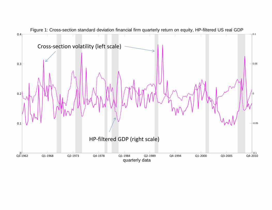
The first calibration target in Table 2 is based on the evidence in Figure 1. That figure

reproduces data constructed in Ferreira (2012). Each quarterly observation in the figure is the

cross-sectional standard deviation of the quarterly rate of return on equity for financial firms

in the CRSP data base. The sample mean of those observations is 0.2, after rounding. The

analog in our model of the volatility measure in Figure 1 is sb in (10). We calibrate the model

so that in steady state, sb = 0.20. The cyclical properties of the volatility data, as well as

HP-filtered GDP data in Figure 1 are discussed in a later section.

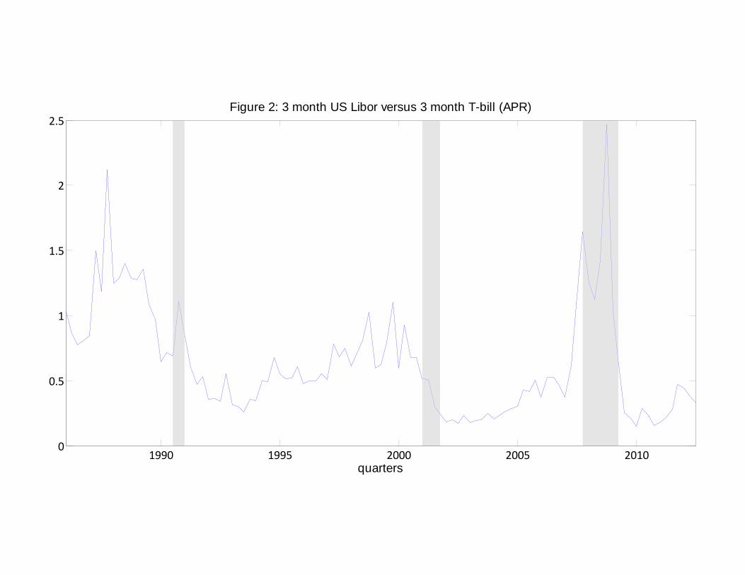
Our second calibration target in Table 2 is the interest rate spread paid by financial firms.

We associate the interest rate spread in the data with Rdg − R in our model. Loosely, we

have in mind that Rdg is the interest rate on the face of the loan contract.

14 The 60 annual

14The return, Rdg,t fluctuates with aggregate uncertainty in our model. In this respect, it does not look likethe rate of return on the face of a loan document.

18

basis point interest rate spread in Table 2 is the sample average of the data on spreads in

Figure 2. That figure displays quarterly data on the spread on 3 month loans, measured by

the London Interbank Offer Rate, over the rate on 3-month US government securities. The

data are reported in annual percent terms.

The third calibration target is leverage, L, which we set to 20. We based this on sample

leverage data reported in CGFS (2009, Graph 3). According to the results reported there, the

leverage of large US investment banks averaged around 25 since 1995 and the leverage of US

commercial banks averaged around 14 over the period.15 Our value, L = 20, is a rough average

of the two.

For the remaining calibration targets we use the average growth of US per capita GDP and

the average decline in US durable good prices. We set the allocative effi ciency of the financial

system in steady state to unity. We suspect that this is in the nature of a normalization. Finally,

we set the fixed cost in the production function so that profits of the intermediate good firms

in steady state are zero. We do not allow entry or exit of these firms, and the implausibility

of this assumption is perhaps minimized with the zero steady state profit assumption.

The parameters pertaining to the financial sector that remain to be determined are b and γ.

The parameter, b, is important in our analysis. If b is suffi ciently low, then the unobserved and

observed equilibria are similar and the essential mechanism emphasized in this paper is absent.

With low b, our baseline model inherits the property of the observable effort equilibrium, that

binding leverage reduces social welfare. If b is too high, then the incentive to exert effort is

substantial and there ceases to exist an interior equilibrium with p (e) < 1 in the baseline

model. We balance these two extremes by setting b = 0.3. With b = 0.2, social welfare falls

when leverage is restricted by a very modest amount, to 19.999. The parameter, γ, resembles

a similar object in Bernanke, Gertler and Gilchrist (1999), who assign a value of 0.98 to it.

We found that with such a large value of γ, the dynamic response of variables to a monetary

policy shock is very different from the results based on vector autoregressions (VARs) reported

in CEE. In particular, a jump in the monetary policy shock in (24) drives inflation and output

up, rather than down. We are still exploring the economic reasons for this result. However,

we noticed that with γ = 0.85, the impulse responses to a monetary policy shock appear more

nearly in line with the results reported in CEE. This is why we chose the value, γ = 0.85. We

are investigating what the implications of micro data may be for the value of this parameter.

The parameters in Panel B were assigned values that are standard in the literature. The

steady state inflation rate corresponds roughly to the actual US experience in recent decades.

15The data are base on information about Bear Stearns, Goldman Sachs, Lehman Brothers, Merrill Lynchand Morgan Stanley.

19

The Calvo sticky price and wage parameters imply that prices and wages on average remain

unchanged for about a year. Similarly, the parameter values in Panel C are also fairly standard.

4.2 The Steady State Effects of Leverage

We consider the impact on welfare and other variables of imposing a binding leverage restric-

tion. The results are reported in Table 3. The first column of numbers displays the steady

state properties of our baseline model, the unobservable effort model without any leverage

restrictions. In that model, the assets of the financial system are 20 times its net worth. The

second column of numbers shows what happens to the steady state of the model when all pa-

rameter are held at their values in Table 1, but a binding leverage restriction of 17 is imposed.

The last two columns of numbers report the same results as in the first two columns, but they

apply to the version of our model in which effort is observable. We first consider the results

for the unobserved effort version of the model.

When leverage restrictions are imposed, Table 3 indicates that bank borrowing, d, declines.

A consequence of this is that the interest rate spread on banks falls. To gain intuition into this

result, we can see from the fact that the multiplier, ν, on the cash constraint, (3), is positive,

that the cash constraint is binding (for ν, see (9)). This means that the creditors of banks

with poorly performing assets must share in the losses, i.e., Rdb is low. However, given the zero

profit condition of mutual funds, (13), it follows that Rdg must be high. That is, R

db < R and

Rdg > R. We can see from (3) that, for given Rb and bank net worth, creditors of ex post bad

banks suffer fewer losses the smaller are their deposits. This is why the value of Rdb that solves

(3) with equality increases with lower deposits. This in turn implies, via the mutual funds’

zero profit condition that Rdg falls towards R as d falls. Thus, deposit rates fluctuate less with

the performance of bank portfolios with smaller d. This explains why the interest rate spread

falls from 60 basis points in the baseline model to 21 basis points with the imposition of the

leverage restriction. A closely related result is that ν falls with the introduction of the binding

leverage constraint.

The reduction in the interest rate spread faced by banks helps to improve the effi ciency of

the economy by giving banks an incentive to increase e (see (8)). But these effects alone only

go part way in explaining the full impact of imposing a leverage restriction on this economy.

There is also an important general equilibrium, dynamic effect of the leverage restriction that

operates via its impact on banker net worth.

To understand this general equilibrium effect, we observe that a leverage restriction in effect

allows banks to collude and behave like monopsonists. Deposits are a key input for banks and

20

unregulated competition drives the profits that banks earn on deposits to zero. We can see this

from the d equation in (9). That equation shows that in an unregulated banking system, the

profits earned by issuing deposits are zero in expectation. This zero profit condition crucially

depends on banks being able to expand deposits in case they earn positive profits on them.

When a binding leverage restriction is imposed, this competitive mechanism is short-circuited.

The d equation in (9) is replaced by (16), where Λ ≥ 0 is the multiplier on the leverage

constraint in the banker problem. When this multiplier is positive the bankers make positive

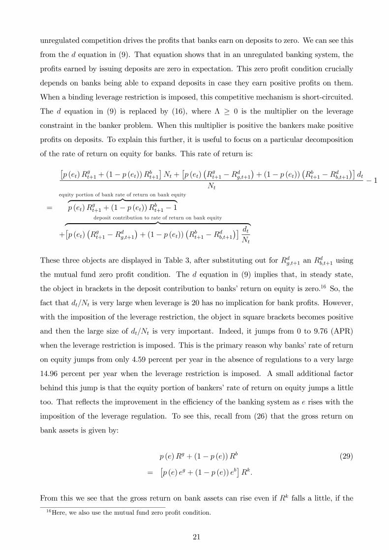
profits on deposits. To explain this further, it is useful to focus on a particular decomposition

of the rate of return on equity for banks. This rate of return is:[p (et)R

gt+1 + (1− p (et))R

bt+1

]Nt +

[p (et)

(Rgt+1 −Rd

g,t+1

)+ (1− p (et))

(Rbt+1 −Rd

b,t+1

)]dt

Nt

− 1

=

equity portion of bank rate of return on bank equity︷ ︸︸ ︷p (et)R

gt+1 + (1− p (et))R

bt+1 − 1

+

deposit contribution to rate of return on bank equity︷ ︸︸ ︷[p (et)

(Rgt+1 −Rd

g,t+1

)+ (1− p (et))

(Rbt+1 −Rd

b,t+1

)] dtNt

These three objects are displayed in Table 3, after substituting out for Rdg,t+1 an R

db,t+1 using

the mutual fund zero profit condition. The d equation in (9) implies that, in steady state,

the object in brackets in the deposit contribution to banks’return on equity is zero.16 So, the

fact that dt/Nt is very large when leverage is 20 has no implication for bank profits. However,

with the imposition of the leverage restriction, the object in square brackets becomes positive

and then the large size of dt/Nt is very important. Indeed, it jumps from 0 to 9.76 (APR)

when the leverage restriction is imposed. This is the primary reason why banks’rate of return

on equity jumps from only 4.59 percent per year in the absence of regulations to a very large

14.96 percent per year when the leverage restriction is imposed. A small additional factor

behind this jump is that the equity portion of bankers’rate of return on equity jumps a little

too. That reflects the improvement in the effi ciency of the banking system as e rises with the

imposition of the leverage regulation. To see this, recall from (26) that the gross return on

bank assets is given by:

p (e)Rg + (1− p (e))Rb (29)

=[p (e) eg + (1− p (e)) eb

]Rk.

From this we see that the gross return on bank assets can rise even if Rk falls a little, if the

16Here, we also use the mutual fund zero profit condition.

21

allocative effi ciency of the banking system improves enough.17

With the high rate of profit it is not surprising that in the new steady state associated

with a leverage restriction, bank net worth is higher. Indeed, it is a substantial 17 percent

higher. This effect on bank net worth mitigates one of the negative consequence of the leverage

restriction. We can see this from (8), which shows that banker effort is not just decreasing

with an increased spread between Rdb an R

dg, but it is also a function of the total quantity of

assets under management. Thus, the bank profits occasioned by the imposition of leverage

restrictions raise banker net worth and mitigate the negative impact on banker effi ciency of a

fall in deposits.

As a way of summarizing the results in Table 3 for the unobserved effort model of this

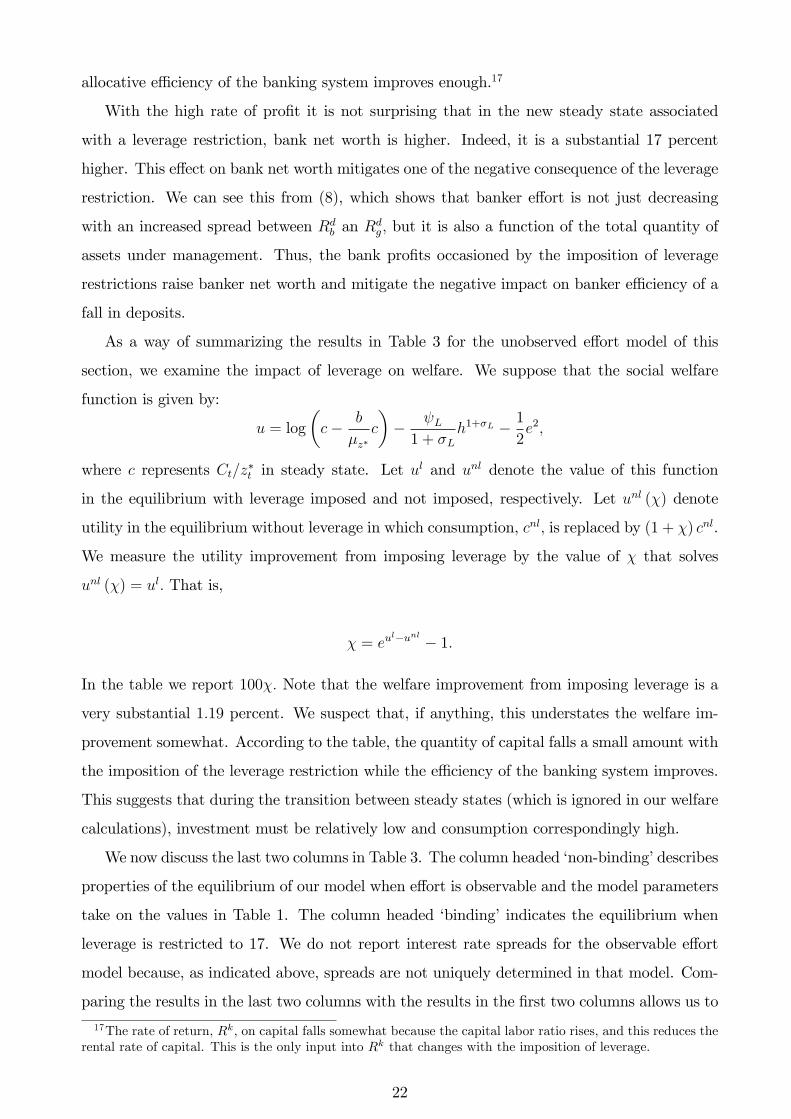
section, we examine the impact of leverage on welfare. We suppose that the social welfare

function is given by:

u = log

(c− b

µz∗c

)− ψL

1 + σLh1+σL − 1

2e2,

where c represents Ct/z∗t in steady state. Let ul and unl denote the value of this function

in the equilibrium with leverage imposed and not imposed, respectively. Let unl (χ) denote

utility in the equilibrium without leverage in which consumption, cnl, is replaced by (1 + χ) cnl.

We measure the utility improvement from imposing leverage by the value of χ that solves

unl (χ) = ul. That is,

χ = eul−unl − 1.

In the table we report 100χ. Note that the welfare improvement from imposing leverage is a

very substantial 1.19 percent. We suspect that, if anything, this understates the welfare im-

provement somewhat. According to the table, the quantity of capital falls a small amount with

the imposition of the leverage restriction while the effi ciency of the banking system improves.

This suggests that during the transition between steady states (which is ignored in our welfare

calculations), investment must be relatively low and consumption correspondingly high.

We now discuss the last two columns in Table 3. The column headed ‘non-binding’describes

properties of the equilibrium of our model when effort is observable and the model parameters

take on the values in Table 1. The column headed ‘binding’indicates the equilibrium when

leverage is restricted to 17. We do not report interest rate spreads for the observable effort

model because, as indicated above, spreads are not uniquely determined in that model. Com-

paring the results in the last two columns with the results in the first two columns allows us to

17The rate of return, Rk, on capital falls somewhat because the capital labor ratio rises, and this reduces therental rate of capital. This is the only input into Rk that changes with the imposition of leverage.

22

highlight the central role in our analysis played by the assumption that effort is not observable.

The welfare results in the table provide two ways to summarize the results.

First, note that imposing a leverage restriction on the model when effort is observed implies

a very substantial 2.70 percent drop in welfare.18 Evidently, leverage restrictions are counter-

productive when effort is observable. Second, the results indicate that the lack of observability

of effort implies a substantial reduction in welfare. In the absence of a leverage restriction, the

welfare gain from making effort observable is 6.11 percent.19 When a binding leverage limit of

17 is in place, then the welfare gain from making effort observable is also a substantial 2.03

percent.20

We now discuss why it is that the observable effort equilibrium is so much better than the

equilibrium in which effort is not observable. We then sum up by pointing out that the benefits

of the leverage restriction on the unobserved effort economy explaining what it is about the

leverage restriction that improves welfare.

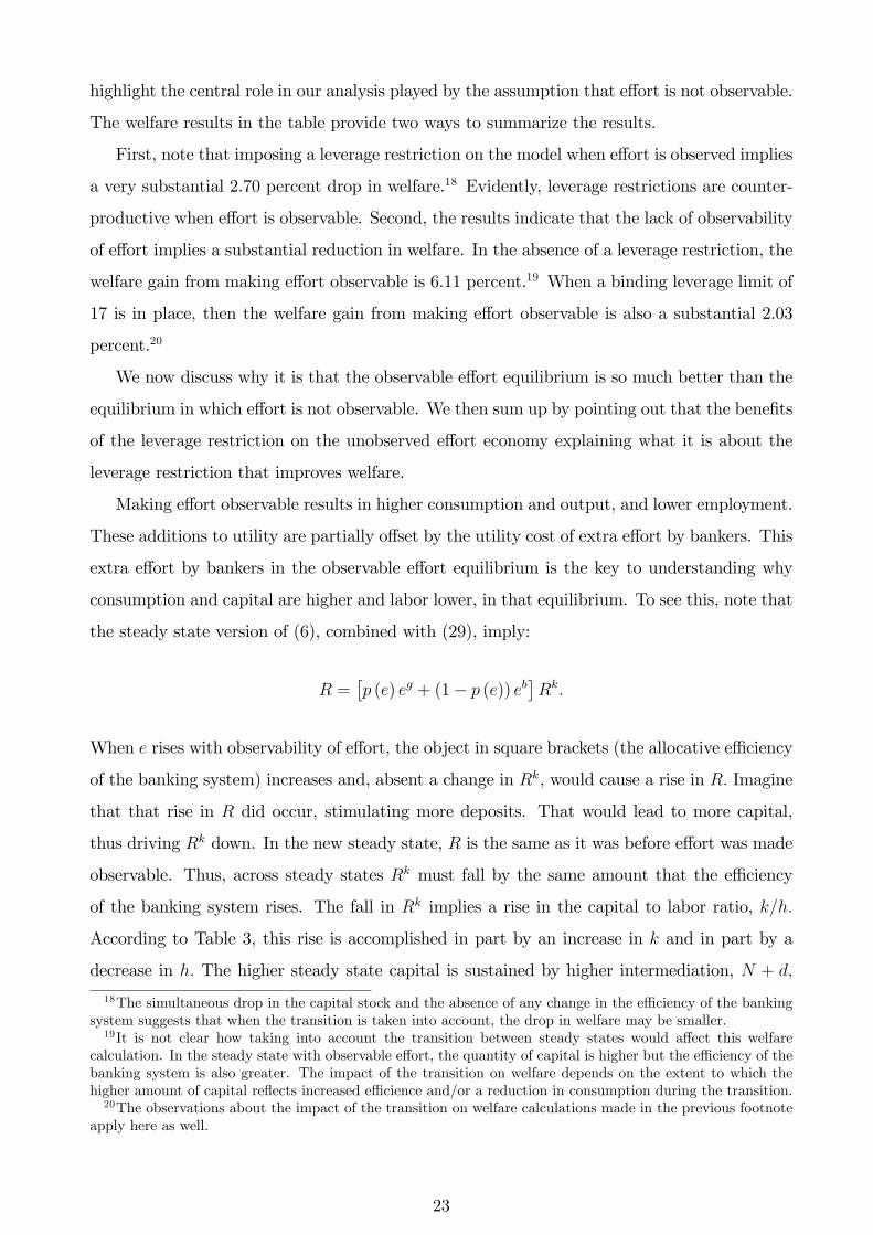
Making effort observable results in higher consumption and output, and lower employment.

These additions to utility are partially offset by the utility cost of extra effort by bankers. This

extra effort by bankers in the observable effort equilibrium is the key to understanding why

consumption and capital are higher and labor lower, in that equilibrium. To see this, note that

the steady state version of (6), combined with (29), imply:

R =[p (e) eg + (1− p (e)) eb

]Rk.

When e rises with observability of effort, the object in square brackets (the allocative effi ciency

of the banking system) increases and, absent a change in Rk, would cause a rise in R. Imagine

that that rise in R did occur, stimulating more deposits. That would lead to more capital,

thus driving Rk down. In the new steady state, R is the same as it was before effort was made

observable. Thus, across steady states Rk must fall by the same amount that the effi ciency

of the banking system rises. The fall in Rk implies a rise in the capital to labor ratio, k/h.

According to Table 3, this rise is accomplished in part by an increase in k and in part by a

decrease in h. The higher steady state capital is sustained by higher intermediation, N + d,

18The simultaneous drop in the capital stock and the absence of any change in the effi ciency of the bankingsystem suggests that when the transition is taken into account, the drop in welfare may be smaller.19It is not clear how taking into account the transition between steady states would affect this welfare

calculation. In the steady state with observable effort, the quantity of capital is higher but the effi ciency of thebanking system is also greater. The impact of the transition on welfare depends on the extent to which thehigher amount of capital reflects increased effi cience and/or a reduction in consumption during the transition.20The observations about the impact of the transition on welfare calculations made in the previous footnote

apply here as well.

23

and this primarily reflects a higher level of deposits.21 Imposing the leverage restriction on the

unobserved effort economy moves consumption, employment and effort in the same direction

that making effort observable does. This is why imposing the leverage restriction raises welfare.

4.3 Dynamic Properties of the Model

In this section we consider the dynamic effects of a monetary policy shock and four financial

shocks.

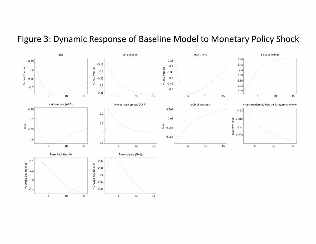
4.3.1 Monetary Policy Shock

Figure 3 displays the responses in our baseline model to a 25 basis point shock to monetary

policy. First, consider the standard macroeconomic variables. The shock has a persistent,

hump-shaped and long-lived effect on output, consumption and investment. The maximal

decline of 0.3 and 0.5 percentage points, respectively, in GDP and investment occur after

about two years. In the case of consumption the maximal decline occurs three years after

the shock and the maximal decline is a little over 0.3 percent. Inflation drops a modest 8

annualized basis points. Unlike the pattern reported in CEE, the response in inflation does

not display a hump-shape. However, direct comparison between the results in Figure 3 and

VAR-based estimates of the effects of monetary policy shocks reported in CEE and other places

is not possible. The latter estimates often assume that aggregate measures of economic activity

and prices and wages are predetermined within the quarter to a monetary policy shock. In

our model, this identifying assumption is not satisfied. One way to see this is to note that

the actual rise in the interest rate is only 15 basis points in the period of the shock. The

fact that the interest rate does not rise the full 25 basis points of the policy shock reflects the

immediate negative impact on the interest rate of the fall in output and inflation. Still, it seems

like a generally positive feature of the model that the implied impulse responses correspond,

in a rough qualitative sense, to the implications of VAR studies for aggregate variables and

inflation.

Now, consider the impact on financial variables. The reduction in output and investment

reduces Rk by two channels: it reduces the rental rate of capital and the value of capital, Pk′ .

Both of these have the effect of reducing bank net worth. The reduction in bank net worth

leads to a tightening of the cash constraint, (3). The result is that the interest rate spread

on banks increases and banker effort declines. That is, p (e) falls 70 basis points. This in

turn is manifest in a rise in the cross-sectional dispersion of bank equity returns. Interestingly,

21In the case with no leverage restriction, the rise in N + d is entirely due to a rise in d.

24

cross-sectional dispersion in the rate of return on financial firm equity is countercyclical in the

data (see Figure 1). Finally, bank assets, N + d, and bank liabilities, d, both decline.

The relative size of the decline in N + d and in d is of some interest. To pursue this, it is

useful to focus on a particular decomposition of the percent change in bank leverage. Let ∆x

denote (x− xs) /xs, where xs is a reference value (perhaps its lagged value) of a variable, x.

Then, letting L denote bank leverage, (N + d) /N, we have22

∆L = (L− 1) [∆d−∆ (N + d)] .

Using this expression we can infer from Figure 3 that our model implies a rise in leverage in

the wake of a monetary-policy induced contraction. Recent literature suggests this implication

is counterfactual (see Adrian, Colla and Shin (2012)). We suspect that a version of the model

could be constructed in which credit responds more and net worth less, so that leverate is

procyclical.

4.3.2 Financial Shocks

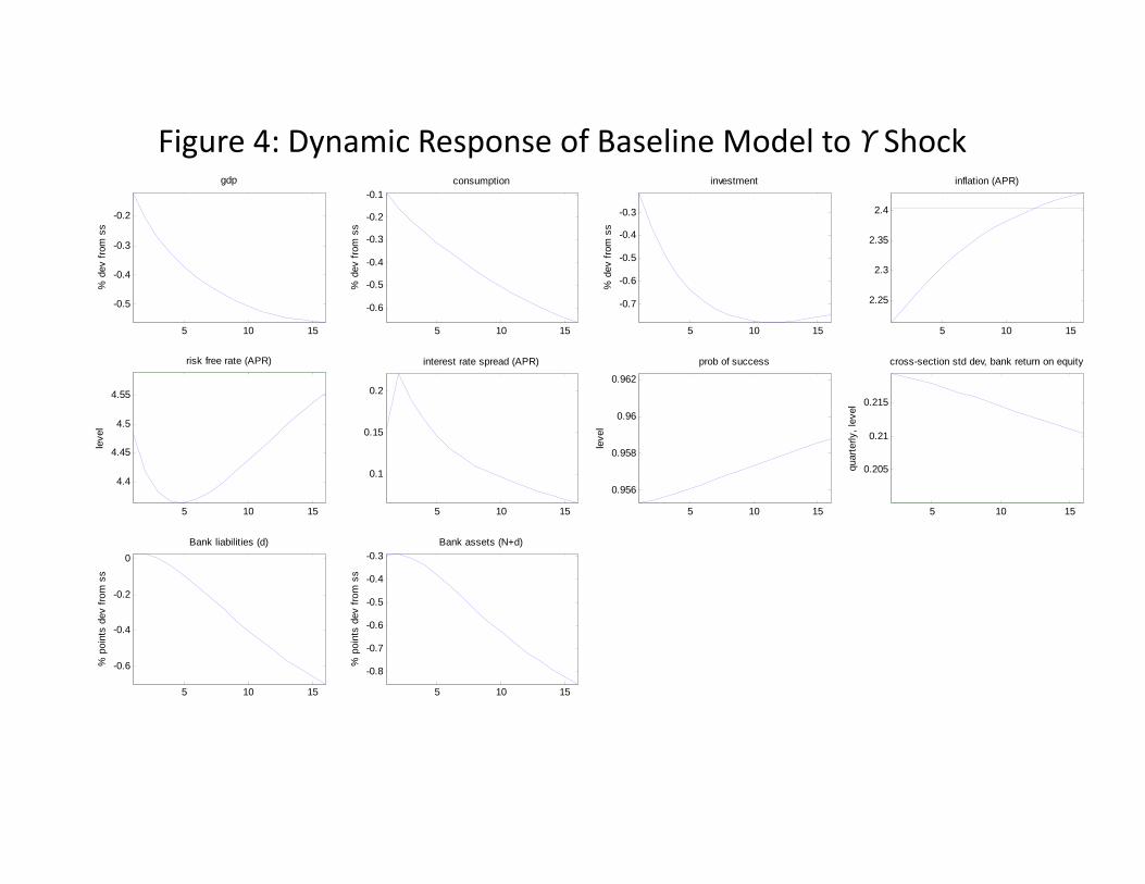
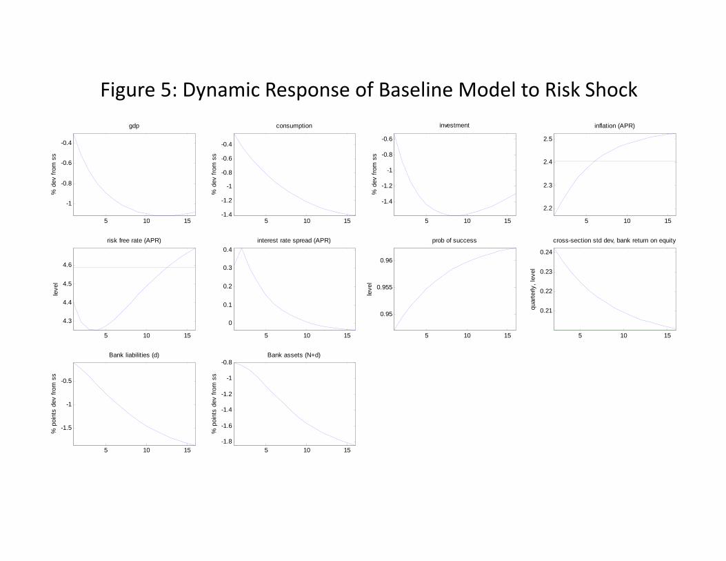
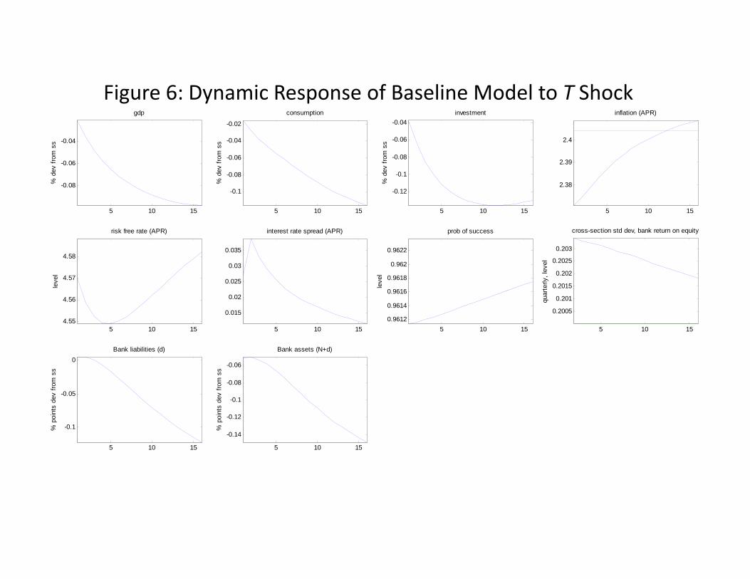
The dynamic responses of the model variables to our three financial shocks are displayed

in Figures 4, 5 and 6. A notable feature of these figures is how similar they are, at least

qualitatively. In each case, consumption, investment, output, inflation and the risk free rate all

fall in response to the shock. The interest rate spread rises and the cross-sectional dispersion in

bank equity returns jumps as p (e) falls. Finally, bank assets and liabilities both fall. However,

the former fall by a greater percent, so that leverage is countercyclical in each case. It is

perhaps not surprising that the risk shock has the greatest quantitative impact on p (e) .

5 Conclusion

Bank leverage has received considerable attention in recent years. Several questions have been

raised about leverage:

22Note that

∆ (N + d) =N

N + d∆N +

d

N + d∆d,

so that

∆N =N + d

N∆ (N + d)− d

N∆d.

Also,∆L = ∆ (N + d)−∆N.

The formula in the text follows by substituting out for ∆N from the first expression.

25

• Should bank leverage be restricted, and how should those restrictions be varied over the

business cycle?

• How should monetary policy react to bank leverage, if at all?

This paper describes an environment that can in principle be used to shed light on these

questions. We have presented some preliminary results by studying the implications for leverage

in steady state. We showed that steady state welfare improves substantially with a binding

welfare restriction. There are several ways to understand the economics of this result. We

pursue one way in this paper. Bigio (2012a) takes an alternative approach, in which he relates

the improvement in welfare to the operation of a pecuniary externality. Either way, leverage

restrictions help to correct a problem in the private economy. For this reason, we think the

model environment is an interesting one for studying the questions listed above.

26

References

[1] Adrian, Tobias, Paolo Colla and Hyun Song Shin, forthcoming, “Which Financial Fric-tions? Parsing the Evidence from the Financial Crisis of 2007-9,” in NBER Macroeco-nomics Annual 2012.

[2] Andolfatto, David, 1996, “Business Cycles and Labor Market Search”, American Eco-nomic Review, Vol. 86, pages 112-132.

[3] Bigio, Saki, 2012, “Financial Risk Capacity,”manuscript, May 31.

[4] Bigio, Saki, 2012a, “Discussion of Christiano and Ikeda,”XVI Annual Conference of theCentral Bank of Chile, “Macroeconomics and Financial Stability: Challenges for MonetaryPolicy,”November 15-16, 2012.

[5] Bernanke, Ben, Mark Gertler and Simon Gilchrist, 1999, “The Financial Accelerator ina Quantitative Business Cycle Framework,”in Taylor, J. B. and M. Woodford (editors),Handbook of Macroeconomics, Volume 1C, chapter 21, Amsterdam: Elsevier Science.

[6] Bloom, Nicholas, 2009, “The Impact of Uncertainty Shocks”Econometrica, 77(3): 623-685.

[7] CGFS, 2009, “The Role of Valuation and Leverage in Procyclicality,”Committee on theGlobal Financial System Papers, no. 34, Bank for International Settlements.

[8] Chari, V.V., and Patrick J. Kehoe, 2012, “Bailouts, Time Inconsistency, and OptimalRegulation”, manuscript, University of Minnesota.

[9] Christiano, Lawrence J., Martin Eichenbaum and Charles Evans. 2005. “Nominal Rigidi-ties and the Dynamic Effects of a Shock to Monetary Policy.”Journal of Political Econ-omy, 113(1): 1-45.

[10] Christiano, Lawrence J., Roberto Motto, and Massimo Rostagno, 2012, “Risk Shocks,”manuscript.

[11] Ferreira, Thiago R. T., 2012, “Financial Volatility and Economic Activity”, manuscriptin preparation, Northwestern University.

[12] Gertler, Mark, Nobuhiro Kiyotaki and Albert Queralto, 2011, “Financial Crises, BankRisk Exposure and Government Financial Policy,”manuscript, May.

[13] Jermann, Urban and Vincenzo Quadrini, 2011, “Macroeconomic Effects of FinancialShocks”, American Economic Review, forthcoming.

[14] Kehrig, Matthias, 2011, “The Cyclicality of Productivity Dispersion,”unpublished man-uscript, University of Texas at Austin.

[15] Smets, Frank and Raf Wouters. 2007, “Shocks and Frictions in US Business Cycles: ABayesian DSGE Approach,”American Economic Review, 97(3): 586-606.

27

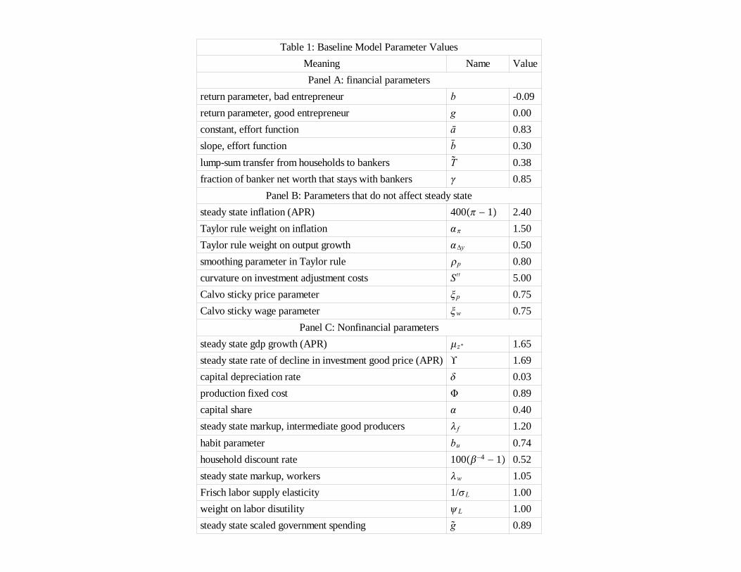
Table 1: Baseline Model Parameter ValuesMeaning Name ValuePanel A: financial parameters

return parameter, bad entrepreneur b -0.09return parameter, good entrepreneur g 0.00constant, effort function ā 0.83slope, effort function b 0.30lump-sum transfer from households to bankers T 0.38fraction of banker net worth that stays with bankers 0.85

Panel B: Parameters that do not affect steady statesteady state inflation (APR) 400 − 1 2.40Taylor rule weight on inflation 1.50Taylor rule weight on output growth Δy 0.50smoothing parameter in Taylor rule p 0.80curvature on investment adjustment costs S′′ 5.00Calvo sticky price parameter p 0.75Calvo sticky wage parameter w 0.75

Panel C: Nonfinancial parameterssteady state gdp growth (APR) z∗ 1.65steady state rate of decline in investment good price (APR) 1.69capital depreciation rate 0.03production fixed cost 0.89capital share 0.40steady state markup, intermediate good producers f 1.20habit parameter bu 0.74household discount rate 100−4 − 1 0.52steady state markup, workers w 1.05Frisch labor supply elasticity 1/L 1.00weight on labor disutility L 1.00steady state scaled government spending g 0.89

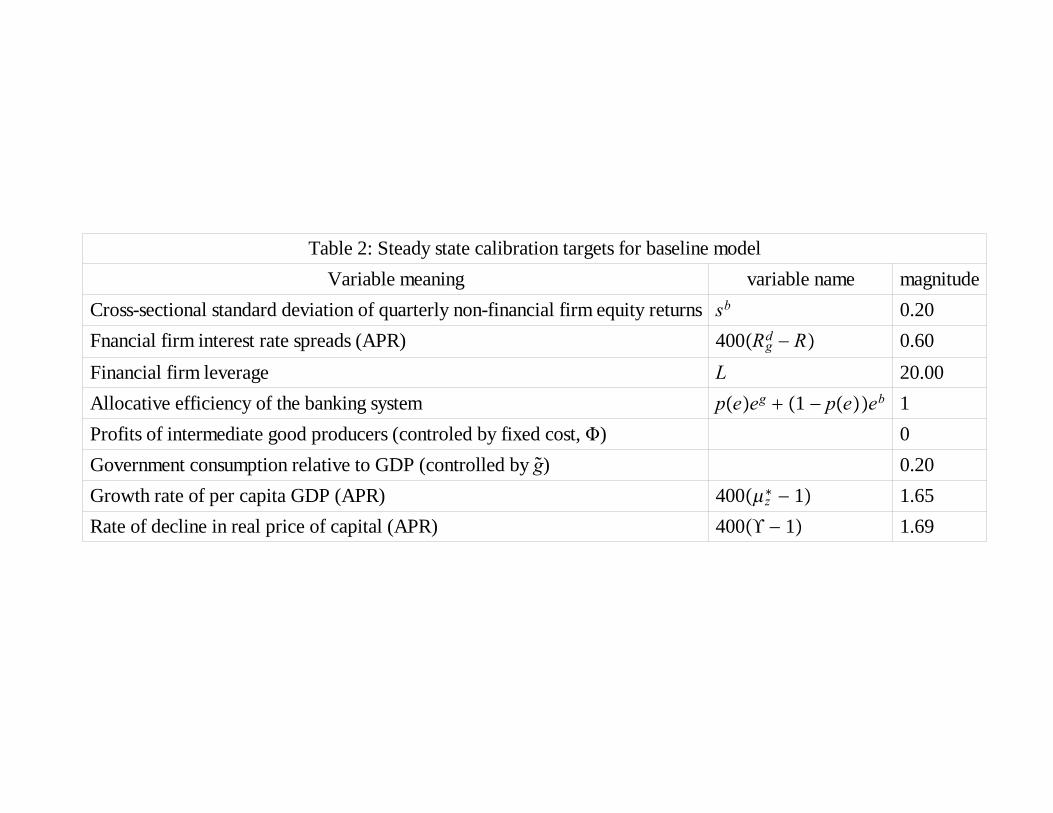
Table 2: Steady state calibration targets for baseline modelVariable meaning variable name magnitude

Cross-sectional standard deviation of quarterly non-financial firm equity returns sb 0.20Fnancial firm interest rate spreads (APR) 400Rgd − R 0.60Financial firm leverage L 20.00Allocative efficiency of the banking system peeg 1 − peeb 1Profits of intermediate good producers (controled by fixed cost, ) 0Government consumption relative to GDP (controlled by g) 0.20Growth rate of per capita GDP (APR) 400z∗ − 1 1.65Rate of decline in real price of capital (APR) 400 − 1 1.69

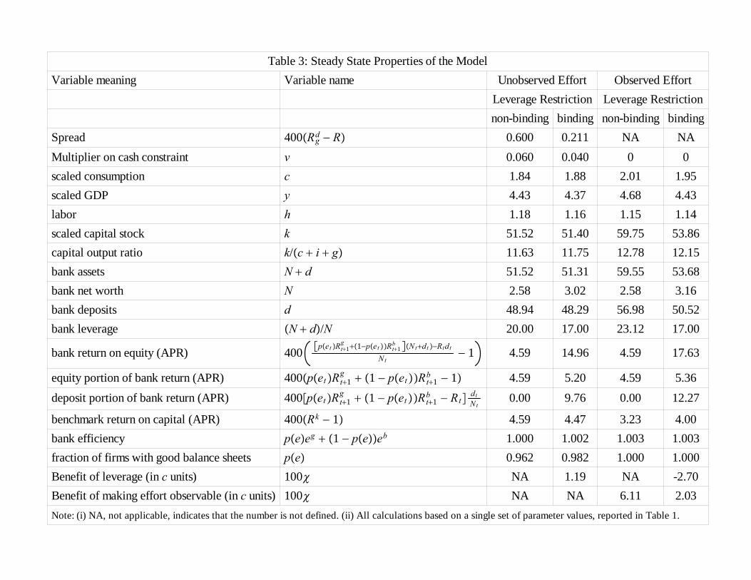
Table 3: Steady State Properties of the ModelVariable meaning Variable name Unobserved Effort Observed Effort

Leverage Restriction Leverage Restrictionnon-binding binding non-binding binding

Spread 400Rgd − R 0.600 0.211 NA NAMultiplier on cash constraint v 0.060 0.040 0 0scaled consumption c 1.84 1.88 2.01 1.95scaled GDP y 4.43 4.37 4.68 4.43labor h 1.18 1.16 1.15 1.14scaled capital stock k 51.52 51.40 59.75 53.86capital output ratio k/c i g 11.63 11.75 12.78 12.15bank assets N d 51.52 51.31 59.55 53.68bank net worth N 2.58 3.02 2.58 3.16bank deposits d 48.94 48.29 56.98 50.52bank leverage N d/N 20.00 17.00 23.12 17.00

bank return on equity (APR) 400 pet Rt1g 1−pet Rt1

b Ntdt −RtdtNt

− 1 4.59 14.96 4.59 17.63

equity portion of bank return (APR) 400petRt1g 1 − petRt1

b − 1 4.59 5.20 4.59 5.36deposit portion of bank return (APR) 400petRt1

g 1 − petRt1b − Rt dtNt 0.00 9.76 0.00 12.27

benchmark return on capital (APR) 400Rk − 1 4.59 4.47 3.23 4.00bank efficiency peeg 1 − peeb 1.000 1.002 1.003 1.003fraction of firms with good balance sheets pe 0.962 0.982 1.000 1.000Benefit of leverage (in c units) 100 NA 1.19 NA -2.70Benefit of making effort observable (in c units) 100 NA NA 6.11 2.03Note: (i) NA, not applicable, indicates that the number is not defined. (ii) All calculations based on a single set of parameter values, reported in Table 1.

Q3‐1962 Q1‐1968 Q2‐1973 Q4‐1978 Q1‐1984 Q2‐1989 Q4‐1994 Q1‐2000 Q3‐2005 Q4‐20100

0.1

0.2

0.3

0.4

quarterly data

Figure 1: Cross-section standard deviation financial firm quarterly return on equity, HP-filtered US real GDP

-0.1

-0.05

0

0.05

0.1

Cross‐section volatility (left scale)

HP‐filtered GDP (right scale)

1990 1995 2000 2005 20100

0.5

1

1.5

2

2.5Figure 2: 3 month US Libor versus 3 month T-bill (APR)

quarters

5 10 15

-0.3

-0.25

-0.2

-0.15

gdp

% d

ev fr

om s

s

5 10 15-0.35

-0.3

-0.25

-0.2

-0.15

consumption

% d

ev fr

om s

s5 10 15

-0.5

-0.45

-0.4

-0.35

-0.3

-0.25

investment

% d

ev fr

om s

s

5 10 15

2.32

2.34

2.36

2.38

2.4

2.42

2.44

inflation (APR)

5 10 15

4.6

4.65

4.7

4.75

risk free rate (APR)

leve

l

5 10 15-0.1

0

0.1

0.2

interest rate spread (APR)

5 10 15

0.956

0.958

0.96

0.962

prob of success

leve

l

5 10 15

0.205

0.21

0.215

0.22

cross-section std dev, bank return on equity

quar

terly

, lev

el

5 10 15

-0.4

-0.3

-0.2

-0.1

Bank liabilities (d)

% p

oint

s de

v fro

m s

s

5 10 15

-0.44

-0.42

-0.4

-0.38

-0.36

Bank assets (N+d)

% p

oint

s de

v fro

m s

s

Figure 3: Dynamic Response of Baseline Model to Monetary Policy Shock

5 10 15

-0.5

-0.4

-0.3

-0.2

gdp

% d

ev fr

om s

s

5 10 15

-0.6

-0.5

-0.4

-0.3

-0.2

-0.1consumption

% d

ev fr

om s

s

5 10 15

-0.7

-0.6

-0.5

-0.4

-0.3

investment

% d

ev fr

om s

s

5 10 15

2.25

2.3

2.35

2.4

inflation (APR)

5 10 15

4.4

4.45

4.5

4.55

risk free rate (APR)

leve

l

5 10 15

0.1

0.15

0.2

interest rate spread (APR)

5 10 15

0.956

0.958

0.96

0.962

prob of success

leve

l

5 10 15

0.205

0.21

0.215

cross-section std dev, bank return on equity

quar

terly

, lev

el

5 10 15

-0.6

-0.4

-0.2

0Bank liabilities (d)

% p

oint

s de

v fro

m s

s

5 10 15

-0.8

-0.7

-0.6

-0.5

-0.4

-0.3Bank assets (N+d)

% p

oint

s de

v fro

m s

s

Figure 4: Dynamic Response of Baseline Model to ϒ Shock

5 10 15

-1

-0.8

-0.6

-0.4

gdp

% d

ev fr

om s

s

5 10 15-1.4

-1.2

-1

-0.8

-0.6

-0.4

consumption

% d

ev fr

om s

s5 10 15

-1.4

-1.2

-1

-0.8

-0.6

investment

% d

ev fr

om s

s

5 10 15

2.2

2.3

2.4

2.5

inflation (APR)

5 10 15

4.3

4.4

4.5

4.6

risk free rate (APR)

leve

l

5 10 15

0

0.1

0.2

0.3

0.4interest rate spread (APR)

5 10 15

0.95

0.955

0.96

prob of success

leve

l

5 10 15

0.21

0.22

0.23

0.24

cross-section std dev, bank return on equity

quar

terly

, lev

el

5 10 15

-1.5

-1

-0.5

Bank liabilities (d)

% p

oint

s de

v fro

m s

s

5 10 15-1.8

-1.6

-1.4

-1.2

-1

-0.8Bank assets (N+d)

% p

oint

s de

v fro

m s

s

Figure 5: Dynamic Response of Baseline Model to Risk Shock

5 10 15

-0.08

-0.06

-0.04

gdp

% d

ev fr

om s

s

5 10 15

-0.1

-0.08

-0.06

-0.04

-0.02

consumption

% d

ev fr

om s

s5 10 15

-0.12

-0.1

-0.08

-0.06

-0.04investment

% d

ev fr

om s

s

5 10 15

2.38

2.39

2.4

inflation (APR)

5 10 154.55

4.56

4.57

4.58

risk free rate (APR)

leve

l

5 10 15

0.015

0.02

0.025

0.03

0.035

interest rate spread (APR)

5 10 150.9612

0.9614

0.9616

0.9618

0.962

0.9622

prob of success

leve

l

5 10 15

0.2005

0.201

0.2015

0.202

0.2025

0.203

cross-section std dev, bank return on equity

quar

terly

, lev

el

5 10 15

-0.1

-0.05

0Bank liabilities (d)

% p

oint

s de

v fro

m s

s

5 10 15

-0.14

-0.12

-0.1

-0.08

-0.06

Bank assets (N+d)

% p

oint

s de

v fro

m s

s

Figure 6: Dynamic Response of Baseline Model to T Shock

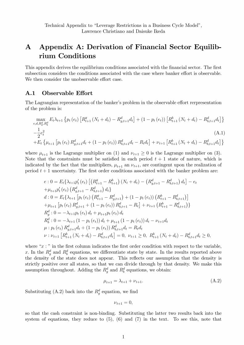
Technical Appendix to “Leverage Restrictions in a Business Cycle Model”,Lawrence Christiano and Daisuke Ikeda

A Appendix A: Derivation of Financial Sector Equilib-rium Conditions

This appendix derives the equilibrium conditions associated with the financial sector. The firstsubsection considers the conditions associated with the case where banker effort is observable.We then consider the unobservable effort case.

A.1 Observable Effort

The Lagrangian representation of the banker’s problem in the observable effort rerpresentationof the problem is:

maxe,d,Rdg ,R

db

Etλt+1

{pt (et)

[Rgt+1 (Nt + dt)−Rd

g,t+1dt]

+ (1− pt (et))[Rbt+1 (Nt + dt)−Rd

b,t+1dt]}

−1

2e2t (A.1)

+Et{µt+1

[pt (et)R

dg,t+1dt + (1− pt (et))R

db,t+1dt −Rtdt

]+ νt+1

[Rbt+1 (Nt + dt)−Rd

b,t+1dt]}

where µt+1 is the Lagrange multiplier on (1) and νt+1 ≥ 0 is the Lagrange multiplier on (3).Note that the constraints must be satisfied in each period t + 1 state of nature, which isindicated by the fact that the multipliers, µt+1 an νt+1, are contingent upon the realization ofperiod t+ 1 uncertainty. The first order conditions associated with the banker problem are:

e : 0 = Et{λt+1p′t (et)

[(Rgt+1 −Rb

t+1

)(Nt + dt)−

(Rdg,t+1 −Rd

b,t+1

)dt]− et

+µt+1p′t (et)

(Rdg,t+1 −Rd

b,t+1

)dt}

d : 0 = Et{λt+1

[pt (et)

(Rgt+1 −Rd

g,t+1

)+ (1− pt (et))

(Rbt+1 −Rd

b,t+1

)]+µt+1

[pt (et)R

dg,t+1 + (1− pt (et))R

db,t+1 −Rt

]+ νt+1

(Rbt+1 −Rd

b,t+1

)}

Rdg : 0 = −λt+1pt (et) dt + µt+1pt (et) dt

Rdb : 0 = −λt+1 (1− pt (et)) dt + µt+1 (1− pt (et)) dt − νt+1dt

µ : pt (et)Rdg,t+1dt + (1− pt (et))R

db,t+1dt = Rtdt

ν : νt+1

[Rbt+1 (Nt + dt)−Rd

b,t+1dt]

= 0, νt+1 ≥ 0, Rbt+1 (Nt + dt)−Rd

b,t+1dt ≥ 0,

where “x : ”in the first column indicates the first order condition with respect to the variable,x. In the Rd

g and Rdb equations, we differentiate state by state. In the results reported above

the density of the state does not appear. This reflects our assumption that the density isstrictly positive over all states, so that we can divide through by that density. We make thisassumption throughout. Adding the Rd

g and Rdb equations, we obtain:

µt+1 = λt+1 + νt+1. (A.2)

Substituting (A.2) back into the Rdg equation, we find

νt+1 = 0,

so that the cash constraint is non-binding. Substituting the latter two results back into thesystem of equations, they reduce to (5), (6) and (7) in the text. To see this, note that

1

µt+1 = λt+1 in the e equation results in a simple cancellation that implies (5). Equation (6) isderived in a similarly simple way. Finally, equation (7) is simply the µ equation repeated.Now suppose we impose a leverage restriction, (15). This only affects the d equation above,

since dt is the only choice variable in the leverage restriction. As a result, our findings, νt+1 = 0and µt+1 = λt+1 are unaffected. That is, the cash constraint remains non-binding and the effortequation remains as in (5). The only change implied by a binding leverage constraint is thatthe 0 in the d equation is replaced by the multiplier on the leverage constraint.

A.2 Unobservable Effort

Given the indicated set of contracts, the Lagrangian representation of the banker’s problemnow is:

max(et,dt,Rdg,t+1,Rdb,t+1)

Etλt+1

{pt (et)

[Rgt+1 (Nt + dt)−Rd

g,t+1dt]

+ (1− pt (et))[Rbt+1 (Nt + dt)−Rd

b,t+1dt]}

−1

2e2t (A.3)

+Etµt+1

[pt (et)R

dg,t+1dt + (1− pt (et))R

db,t+1dt −Rtdt

]+ηt

(et − Etλt+1p

′t (et)

[(Rgt+1 −Rb

t+1

)(Nt + dt)−

(Rdg,t+1 −Rd

b,t+1

)dt])

+Etνt+1

[Rbt+1 (Nt + dt)−Rd

b,t+1dt].

where ηt is the Lagrange multiplier on (8). Note that this multiplier is not contingent on therealization of the period t+1 state of nature since the constraint is on the effort level exerted bythe banker in t. To understand the solution to this problem, consider the first order necessaryconditions associated with the banker problem, (A.3):

e : Etλt+1p′t (et)

[(Rgt+1 −Rb

t+1

)(Nt + dt)−

(Rdg,t+1 −Rd

b,t+1

)dt]

−et + Etµt+1p′t (et)

(Rdg,t+1 −Rd

b,t+1

)dt

+ηt(1− Etλt+1p

′′t (et)

[(Rgt+1 −Rb

t+1

)(Nt + dt)−

(Rdg,t+1 −Rd

b,t+1

)dt])

= 0

d : 0 = Etλt+1pt (et)(Rgt+1 −Rd

g,t+1

)+ Etλt+1 (1− pt (et))

(Rbt+1 −Rd

b,t+1

)+Etµt+1

[pt (et)R

dg,t+1 + (1− pt (et))R

db,t+1 −Rt

]−ηtEtλt+1p

′t (et)

[(Rgt+1 −Rb

t+1

)−(Rdg,t+1 −Rd

b,t+1

)]+ Etνt+1

(Rbt+1 −Rd

b,t+1

)Rdg : −λt+1pt (et) + µt+1pt (et) + ηtλt+1p

′t (et) = 0

Rdb : −λt+1 (1− pt (et)) + µt+1 (1− pt (et))− ηtλt+1p

′t (et)− νt+1 = 0

µ : Rt = pt (et)Rdg,t+1 + (1− pt (et))R

db,t+1

η : et = Etλt+1p′t (et)

[(Rgt+1 −Rb

t+1

)(Nt + dt)−

(Rdg,t+1 −Rd

b,t+1

)dt]

ν : νt+1

[Rbt+1 (Nt + dt)−Rd

b,t+1dt]

= 0, νt+1 ≥ 0,[Rbt+1 (Nt + dt)−Rd

b,t+1dt]≥ 0.

Add the Rdg and Rd

b equations, to obtain (A.2). To simplify the e equation, use (A.2) tosubstitute out µt+1 :

e : Etλt+1p′t (et)

[(Rgt+1 −Rb

t+1

)(Nt + dt)−

(Rdg,t+1 −Rd

b,t+1

)dt]− et

+Et [λt+1 + νt+1] p′t (et)(Rdg,t+1 −Rd

b,t+1

)dt

+ηt(1− Etλt+1p

′′t (et)

[(Rgt+1 −Rb

t+1

)(Nt + dt)−

(Rdg,t+1 −Rd

b,t+1

)dt])

= 0

2

or,

e : Etλt+1p′t (et)

(Rgt+1 −Rb

t+1

)(Nt + dt)− et + Etνt+1p

′t (et)

(Rdg,t+1 −Rd

b,t+1

)dt

+ηt(1− Etλt+1p

′′t (et)

[(Rgt+1 −Rb

t+1

)(Nt + dt)−

(Rdg,t+1 −Rd

b,t+1

)dt])

= 0

Now, make use of p′′t = 0 and the η equation to substitute out for et :

e : Etλt+1p′t (et)

(Rgt+1 −Rb

t+1

)(Nt + dt)− Etλt+1p

′t (et)

[(Rgt+1 −Rb

t+1

)(Nt + dt)−

(Rdg,t+1 −Rd

b,t+1

)dt]

+Etνt+1p′t (et)

(Rdg,t+1 −Rd

b,t+1

)dt + ηt = 0

or,e : Etλt+1p

′t (et)

(Rdg,t+1 −Rd

b,t+1

)dt + Etνt+1p

′t (et)

(Rdg,t+1 −Rd

b,t+1

)dt + ηt = 0

or,e : Et [λt+1 + νt+1] p′t (et)

(Rdg,t+1 −Rd

b,t+1

)dt + ηt = 0.

We now simplify the d equation. From the µ-condition, we delete the third term in dequation and obtain

0 = Etλt+1pt (et)(Rgt+1 −Rd

g,t+1

)+ Etλt+1 (1− pt (et))

(Rbt+1 −Rd

b,t+1

)−ηtEtλt+1p

′t (et)

[(Rgt+1 −Rb

t+1

)−(Rdg,t+1 −Rd

b,t+1

)]+ Etνt+1

(Rbt+1 −Rd

b,t+1

)Use (A.2) to substitute out for µt+1 in the R

dg condition:

νt+1pt (et) + ηtλt+1p′t (et) = 0

Substituting out ηt using Rdg-condition,

−λt+1pt (et) + [λt+1 + νt+1] pt (et) + ηtλt+1p′t (et) = 0

νt+1pt (et) + ηtλt+1p′t (et) = 0 (A.4)

Note that this equation impliesηt ≤ 0.

This is to be expected. The interpretation of this may be seen from (A.3). The sign of ηtsuggests that in the absence of the η constraint, i.e., if ηt = 0, then et would be set in away that makes et greater than the object on the right of the minus sign in the incentiveconstraint. A negative value of ηt in the Lagrangian penalizes such a setting. But, we knowfrom our analysis of the observable effort case (the only difference in this case is that theincentive constraint is absent), that et is greater than the object on the right of the minus signin the η constraint in (A.3) when that constraint is ignored. But, (A.4) has another notableimplication. Suppose, for simplicity, that from the point of view of t, there are two possiblestates of nature in t+ 1, 1 and 2. Then,

ν1t+1pt (et) + ηtλ

1t+1p

′t (et) = 0

ν2t+1pt (et) + ηtλ

2t+1p

′t (et) = 0

We assume that λ1t+1, λ

2t+1, p

′t (et) , pt (et) > 0. Suppose the cash constraint is not binding in

state of nature, 1, so that ν1t+1 = 0. In that case, the first equation says that ηt = 0. But,

the second equation then implies ν2t+1 = 0 too. Thus, if the cash constraint is not binding

in some state of nature for a particular date, then it must not be binding in the other stateeither. If it is binding is one state, ν1

t+1 > 0, then ηt > 0 and it is binding in the other state.Thus, it is either binding in all states at a particular date, or none. This is general. Note from

3

Rdg-condition that

ηt = −νt+1pt (et) / [λt+1p′t (et)] ,

which implies that there exists no solution such that νt+1 = 0 for some states of natureand νt+1 > 0 for others. Intuitively this is because a banker smooths ineffi ciency caused byRdg,t+1 − Rd

b,t+1 > 0 state by state. Suppose Rbt+1 is very low in one state and it is very high

in another. Then, the cash constraint is binding in the low state so that Rdg,t+1 − Rd

b,t+1 > 0.In the high state the banker sets Rd

b,t+1 high enough so that the cash constraint is binding andRdg,t+1 − Rd

b,t+1 < 0. By doing this the banker minimizes Etλt+1p′t (et)

(Rdg,t+1 −Rd

b,t+1

)≥ 0,

which is, loosely speaking, the measure of ineffi ciency.Substituting out for ηt in the revised d equation:

0 = Etλt+1pt (et)(Rgt+1 −Rd

g,t+1

)+ Etλt+1 (1− pt (et))

(Rbt+1 −Rd

b,t+1

)+Etνt+1pt (et)

[(Rgt+1 −Rb

t+1

)−(Rdg,t+1 −Rd

b,t+1

)]+ Etνt+1

(Rbt+1 −Rd

b,t+1

)or,

0 = Etλt+1

[pt (et)

(Rgt+1 −Rd

g,t+1

)+ (1− pt (et))

(Rbt+1 −Rd

b,t+1

)]+Etνt+1

[pt (et)

(Rgt+1 −Rd

g,t+1

)+ (1− pt (et))

(Rbt+1 −Rd

b,t+1

)]or

0 = Et (λt+1 + νt+1)[pt (et)

(Rgt+1 −Rd

g,t+1

)+ (1− pt (et))

(Rbt+1 −Rd

b,t+1

)].

Then, using the µ-condition,

0 = Et (λt+1 + νt+1)[pt (et)R

gt+1 + (1− pt (et))R

bt+1 −Rt

].

Finally, we use (A.2) to substitute out for µt+1 in the Rdg equation, to obtain:

Rdg : νt+1pt (et) + ηtλt+1p

′t (et) = 0.

The optimization conditions derived here are summarized in (9).To gain intuition into this multiplier, consider the case, νt+1 = 0, so that the cash constraint

is not binding and the Rdg condition implies ηt = 0. Since λt+1 + νt+1 > 0 the e-condition then

implies that Rdg,t+1 = Rd

b,t+1 can be the solution (as long as it does not make the cash constraintbinding). Combining this with the µ-condition then implies that

Rdg,t+1 = Rd

b,t+1 = Rt (A.5)

can be the solution. It then follows from the η-condition that:

et = Etλt+1p′t (et)

[(Rgt+1 −Rb

t+1

)(Nt + dt)

], (A.6)

so that banker effort level is effi cient.Now consider the case, νt+1 > 0 for all states of nature. Then, the Rd

g-condition impliesηt < 0 and the e-condition, after substituting out νt+1 using the the Rd

g-condition, implies

Etλt+1p′t (et)

(Rdg,t+1 −Rd

b,t+1

)dt = − ηt

1− ηtp′t(et)

pt(et)

> 0.

The e-condition then shows that banker effort is suboptimal. By continuity, when νt+1 is largethe ineffi ciency of the banking system is great and when it is small, there ineffi ciency is smaller.We think of a ‘crisis time’as one in which νt+1 is large.

4

Given our constraints, we suspect that when the cash constraint is always binding, νt+1 > 0,all state contingent deposit returns Rd

g,t+1, Rdb,t+1,are pinned down. To see why, consider the

case in which there are two aggregate states possible in period t + 1, given period t. Denotethese by 1 and 2 and suppose they have probability, πt and 1−πt, respectively. The µ equationsare:

Rt = pt (et)Rd,1g,t+1 + (1− pt (et))R

d,1b,t+1

Rt = pt (et)Rd,2g,t+1 + (1− pt (et))R

d,2b,t+1

and the ν equations are

Rb,1t+1 (Nt + dt)−Rd,1

b,t+1dt = 0

Rb,2t+1 (Nt + dt)−Rd,2

b,t+1dt = 0

Given the time t realization of variables, this represents four equations in four unknowns.In general, for given Rt, pt (et) these variables are pinned down. If there are more states ofnature, then these equations represent restrictions on the deposit returns. Either way, the statecontingency in the returns does not appear to contribute directly to multiplicity of equilibria,at least when the case constraint is always binding. As a practical matter, we can solve themodel assuming the cash constraint always binds. We can then inspect the multiplier andverify that it is always positive. If ever it is negative that means that the constraint as aninequality is in fact not binding.Consider the issue of the relative magnitude of Rd

b,+1 and Rdg,+1.We suspect that it will not

be true across all states of nature that Rdb,t+1 ≤ Rd

g,t+1. Consider a simple example. Supposethere is an aggregate state where Rb

t+1 = 0. In that state, it must be that Rdb,t+1 = 0 too. In

such a state, assuming Rt > 0, it must be that Rdg,t+1 > Rd

b,t+1. By itself, this spread induces asubstantial ineffi ciency in the e decision (see the η equation). But, the spread affects the choiceof e only by its expected value. If that spread is very large in some state then it does not inducea large ineffi ciency if it is suffi ciently small in another state. We might even imagine that itcould be negative in another state, Rd

b,t+1 > Rdg,t+1. In this case, creditors in effect subsidize

bankers that make positive profits and tax the ones that lose. This obviously has a big positiveincentive effect on e. This possibility should not be a problem for our maintained assumptionthat the cash constraint is non-binding in the g state. To see this, suppose that it is bindingin the b state:

Rbt+1 (Nt + dt)−Rd

b,t+1dt = 0.

By construction, Rgt+1 > Rb

t+1 in all aggregate states. also, in the scenario we are discussing,Rdg,t+1 < Rd

b,t+1. Both guarantee that the cash constraint is not binding in the g state.An interesting feature of the model is that it implies a non-trivial cross-sectional variance

on the returns of banks. In any given period t + 1 state of nature, the cross section mean ofbank returns on equity is:

Rmt+1 = pt (et)

[Rgt+1 (Nt + dt)−Rd

g,t+1dt

Nt

]+ (1− pt (et))

[Rbt+1 (Nt + dt)−Rd

b,t+1dt

Nt

].

To determine the cross sectional standard deviation of bank equity returns, note that in thecross section, in any aggregate state, pt (et) banks each earn

Rgt+1 (Nt + dt)−Rd

g,t+1dt

Nt

5

return on equity. Similarly, 1− pt (et) banks earn a return on equity equal to

Rbt+1 (Nt + dt)−Rd

b,t+1dt

Nt

.

Recall that if a random variable has a binomial distribution and takes on the value xh withprobability p and xl with probability 1 − p, then the variance of that random variable isp (1− p)

(xh − xl

)2. So, the period t cross-sectional standard deviation of bank returns is:

sdt+1 = [pt (et) (1− pt (et))]1/2

[Rgt+1 (Nt + dt)−Rd

g,t+1dt

Nt

−Rbt+1 (Nt + dt)−Rd

b,t+1dt

Nt

]

= [pt (et) (1− pt (et))]1/2 R

gt+1 (Nt + dt)−Rd

g,t+1dt

Nt

,

taking into account our assumption that the cash constraint is binding for bad banks. Notethat pt (et) > 1/2 then the cross sectional standard deviation is decreasing in et.

B Appendix B: Scaling and Miscellaneous Variables

To solve our model, we require that the variables be stationary. To this end, we adopt aparticular scaling of the variables. Because our model satisfies suffi cient conditions for bal-anced growth, when the equilibrium conditions of the model are written in terms of the scaledvariables, only the growth rates and not the levels of the stationary shocks appear. In thisappendix we describe the scaling of the model that is adopted. In addition, we describe themapping from the variables in the scaled model to the variables measured in the data.Let

qt = ΥtPk′,tPt

, yz,t =Ytz+t

, it =It

z+t Υt

, wt ≡Wt

z+t Pt

, pI,t ≡1

ΥtµΥ,t

, PI,t =Pt

ΥtµΥ,t

kt =Kt

z+t−1Υt−1

, rkt = Υtrkt , µ∗z,t =

z+t

z+t−1

, ct =Ctz+t

, λz,t = λtz∗tPt

where rkt Pt denotes the nominal rental rate on capital. Also, rkt denotes the real, unscaled,

rental rate of capital. We do not work with this variable. The rate of inflation in the nominalwage rate is:

πw,t ≡Wt

Wt−1

=wtµ

∗z,tπt

wt−1

.

Consider gdp growth, according to the model.

Y gdpt

z+t

≡ yt = ct +itµΥ,t

+ gt,

or,Y gdpt = ytz

+t ,

so that

∆ log Y gdpt = log Y gdp

t − log Y gdpt−1 = log (yt)− log (yt−1) + log

(z+t

)− log z+

t−1

= log (yt)− log (yt−1) + log µ∗z,t

6

Let Nt denote period t nominal net worth, so that

nt =Nt

Ptz+t

.

Then,

∆ logNt

Pt= log nt − log nt−1 + log µ∗z,t.

Another variable is investment. There is an issue about what units to measure investmentin. Investment times its relative price is given by:

invt ≡It

ΥtµΥ,t

=itz

+t Υt

ΥtµΥ,t

=itz

+t

µΥ,t

,

so that:

∆ log invt ≡ log invt − log invt−1 = log it − log it−1 + log µ∗z,t −(log µΥ,t − log µΥ,t−1

).

The investment goods relative to consumption goods is given by

pI,t ≡1

ΥtµΥ,t

,

so that

∆ log pI,t = −t log Υ + (t− 1) log Υ− log µΥ,t + log µΥ,t−1

= − log Υ− log µΥ,t + log µΥ,t−1.

Also,∆ logCt = log ct − log ct−1 + log µ∗z,t.

The growth rate of the real wage is:

∆ logWt

Pt= log wt − log wt−1 + log µ∗z,t

C Appendix C: Dynamic Equations

Here, we display all the dynamic equilibrium conditions associated with the model.

C.1 Prices

The equations pertaining to prices are:

(1)p∗t −

(1− ξp)(Kp,t

Fp,t

) λf1−λf

+ ξp

(πtπtp∗t−1

) λf1−λf

1−λfλf

= 0 (C.1)

and

(2)Et

{ζc,tλz,tyz,t +

(πt+1

πt+1

) 11−λf

βξpFp,t+1 − Fp,t

}= 0, (C.2)

7

where λz,t denotes λtz∗tPt. Also,

(3)ζc,tλz,tλfyz,tst + βξp

(πt+1

πt+1

) λf1−λf

Kp,t+1 −Kp,t = 0. (C.3)

Note that both these equations involve Fp,t. This reflects that a lot of equations have beensubstituted out. In particular, we have

(4)Fp,t

1− ξp(πtπt

) 11−λf

1− ξp

1−λf

= Kp,t, pt =Kp,t

Fp,t,

where pt is the real price set by price-optimizing firms in period t. This is not a variable ofdirect interest in the analysis.

C.2 Wages

The demand for labor is the solution to the following problem:

maxWt

=lt︷ ︸︸ ︷[∫ 1

0

(ht,i)1λw di

]λw−∫ 1

0

Wt,iht,idi,

where Wt,i is the wage rate of i−type workers and Wt is the wage rate for homogeneous labor,lt. The first order condition is:

ht,i = lt

(Wt

Wt,i

) λwλw−1

.

The wages of non-optimizing unions evolve as follows:

Wj,t = πw,t(µz∗,t

)ιµ(µz∗)

1−ιµWj,t−1, πw,t ≡ (π∗t )ιw1 (πt−1)ιw2 π1−ιw1−ιw2 , (C.4)

Nominal wage growth, πw,t, is:

πw,t =wtµ

∗z,tπt

wt−1

,

where wt denotes the scaled wage rate:

wt ≡Wt

z∗tPt.

The labor input variable that we treat as observed is the sum over the various differenttypes of labor:

ht =

∫ 1

0

hitdi

= ltWλwλw−1t

∫ 1

0

(Wt,i)λw

1−λw di

= ltWλwλw−1t (W ∗

t )λw

1−λw ,

8

where

W ∗t ≡

[∫ 1

0

(Wt,i)λw

1−λw di

] 1−λwλw

=

[(1− ξw) Wt +

∫ξw monopolists that do not reoptimize

(πw,t

(µz∗,t

)ιµ(µz∗)

1−ιµWi,t−1

) λw1−λw di

] 1−λwλw

=

[(1− ξw) Wt + ξw

(πw,t

(µz∗,t

)ιµ(µz∗)

1−ιµW ∗t−1

) λw1−λw

] 1−λwλw

.

Let w∗t ≡ W ∗t /Wt, and use linear homogeneity:

w∗t =

(1− ξw)Wt

Wt

+ ξw

(πw,t

(µz∗,t

)ιµ(µz∗)

1−ιµ

πw,tw∗t−1

) λw1−λw

1−λwλw

,

Wt is the nominal wage set by the 1− ξw wage optimizers in the current period. Rewriting,

w∗t = [(1− ξw)wλw

1−λwt + ξw

(πw,t

(µ∗z,t)ιµ

(µ∗z)1−ιµ

πwtw∗t−1

) λw1−λw

]1−λwλw , (C.5)

where

wt ≡Wt

Wt

. (C.6)

We conclude:ht = lt (w∗t )

λw1−λw . (C.7)

For purposes of evaluating aggregate utility, it is also convenient to have an expression forthe following: ∫ 1

0

h1+σLit di

= l1+σLt W

−λw(1+σL)1−λw

t

∫ 1

0

(Wt,i)λw(1+σL)1−λw di

= l1+σLt W

−λw(1+σL)1−λw

t Wλw(1+σL)1−λw

t ,

where

Wt ≡[∫ 1

0

(Wt,i)λw(1+σL)1−λw di

] 1−λwλw(1+σL)

.

Then,

Wt =

[∫ 1

0

(Wt,i)λw(1+σL)1−λw di

] 1−λwλw(1+σL)

=

[(1− ξw)

(Wt

)λw(1+σL)1−λw

+

∫ξw that change

(Wt,i)λw(1+σL)1−λw di

] 1−λwλw(1+σL)

=

[(1− ξw)

(Wt

)λw(1+σL)1−λw

+ ξw

(πw,t

(µz∗,t

)ιµ(µz∗)

1−ιµ Wt−1

)λw(1+σL)1−λw

] 1−λwλw(1+σL)

.

9

Divide by Wt and make use of the linear homogeneity of the above expression:

Wt

Wt

=

(1− ξw)

(Wt

Wt

)λw(1+σL)1−λw

+ ξw

(πw,t

(µz∗,t

)ιµ(µz∗)

1−ιµ

πw,t

Wt−1

Wt−1

)λw(1+σL)1−λw

1−λw

λw(1+σL)

Define

wt =Wt

Wt

,

so that

wt =

(1− ξw) (wt)λw(1+σL)1−λw + ξw

(πw,t

(µz∗,t

)ιµ(µz∗)

1−ιµ

πw,twt−1

)λw(1+σL)1−λw

1−λw

λw(1+σL)

, (C.8)

using (C.6). We conclude ∫ 1

0

h1+σLit di =

[lt (wt)

λw1−λw

](1+σL)

(C.9)

=

[ht

(wtw∗t

) λw1−λw

](1+σL)

.

using (C.7).The optimality conditions associated with wage-setting are characterized by:

(5)Et{ζc,tλz,t(w∗t )

λwλw−1 ht

(1− τ lt

)λw

(C.10)

+βξw (µz∗)1−ιµ1−λw Et

(µz∗,t+1

) ιµ1−λw−1

(1

πw,t+1

) λw1−λw π

11−λww,t+1

πt+1

Fw,t+1 − Fw,t} = 0

and

(6) Et{ζc,tζt[(w∗t )

λwλw−1 ht

]1+σL+βξw

(πw,t+1

(µ∗z,t+1

)ιµ(µ∗z)

1−ιµ

πwt+1

) λw1−λw (1+σL)

Kw,t+1−Kw,t} = 0.

(7)1

ψL

1− ξw(πw,tπw,t

(µz∗)1−ιµ (µz∗,t)ιµ) 1

1−λw

1− ξw

1−λw(1+σL)

wtFw,t −Kw,t = 0

Optimization by households implies:

wt =

[ψLwt

Kw,t

Fw,t

] 1−λw1−λw(1+σL)

,

so that, using (C.5):

w∗t =

(1− ξw)

[ψLwt

Kw,t

Fw,t

] λw1−λw(1+σL)

+ ξw

(πw,t

(µ∗z,t)ιµ

(µ∗z)1−ιµ

πwtw∗t−1

) λw1−λw

1−λwλw

.

10

We can replace Kw,t/Fw,t with the expression implied by (7) above:

(8) w∗t =

(1− ξw)

1− ξw(πw,tπw,t

(µz∗)1−ιµ (µz∗,t)ιµ) 1

1−λw

1− ξw

λw

+ ξw

(πw,t

(µ∗z,t)ιµ

(µ∗z)1−ιµ

πwtw∗t−1

) λw1−λw

1−λwλw

(C.11)

C.3 Capital Utilization, Marginal Cost, Return on Capital, Invest-ment, Monetary Policy

The first order necessary condition associated with the capital utilization decision is:

1

Υta′ (ut) = rkt ,

or,a′ (ut) = Υtrkt = rkt ,

after scaling. Making use of our assumed utilization cost function, this reduces to:

(9) rkt = rk exp (σa [ut − 1]) ,

where

a (ut) =rk

σa[exp(σa [ut − 1])− 1] .

Also, rk denotes the steady state value of rkt . The above restriction on the a (ut) functionimplies that u = 1 in a steady state. As a result, the steady state is independent of the capitaladjustment costs.Marginal cost is given by:

(10)rkt =αεt[

1 + ψk,tRt

] (Υµ∗z,tLt (w∗t )λwλw−1

utkt

)1−α

st (C.12)

wt =(1− α) εt[1 + ψl,tRt

] (Υµ∗z,tLt (w∗t )λwλw−1

utkt

)−αst,

where ψk,t and ψl,t denote the fraction of the capital services and labor bills, respectively,that must be financed in advance. Combining the last two equations, we obtain the familiarexpression for marginal cost:

(11) st =1

εt

(rkt[1 + ψk,tRt

]α

)α(wt[1 + ψl,tRt

]1− α

)1−α

, (C.13)

where ψk,t = ψl,t = 0. Resource constraint:

(12)a(ut)kt

Υµ∗z,t+ gt + ct +

itµΥ,t

= yz,t (C.14)

11

where gt is an exogenous stochastic process and

(13)kt+1 =

relevant only for financial friction model, drop in CEE version︷ ︸︸ ︷[pt (et) e

gt + (1− pt (et)) ebt] {

(1− δ) 1

µ∗z,tΥkt +

[1− S

(ζ i,t itµ

∗z,tΥ

it−1

)]it

},

(C.15)where it is investment scaled by z∗t Υ

t.Equation defining the nominal non-state contingent rate of interest:

(14)Et{β1

πt+1µ∗z,t+1

ζc,t+1λz,t+1Rt − ζc,tλz,t} = 0 (C.16)

The derivative of utility with respect to consumption is,

(15)Et

[ζc,tλz,t −

µ∗z,tζc,tctµ∗z,t − bct−1

+ bβζc,t+1

ct+1µ∗z,t+1 − bct

]= 0, (C.17)

where ct denotes consumption scaled by z∗t . The following capital first order first order condi-tion is an equilibrium condition in CEE, but not in our model with financial frictions becausein that model households do not accumulate capital:

(16)Et

{−ζc,tλzt +

β

πt+1µ∗z,t+1

ζc,t+1λzt+1Rkt+1

}= 0. (C.18)

In (C.18), Rkt+1 denotes the benchmark rate of return on capital:

(17) Rkt =

utrkt − a(ut) + (1− δ)qt

Υqt−1

πt

where qt denotes the scaled market price of capital, QK′,t :

qt = ΥtQK′,t

Pt.

Equation (17) holds in our financial friction model, as well as in CEE. The investment firstorder condition, (28)

(18) Et{ζc,tλztqt[1− S(

ζ i,tµ∗z,tΥit

it−1

)− S ′(ζ i,tµ

∗z,tΥit

it−1

)ζ i,tµ

∗z,tΥit

it−1

](C.19)

−ζc,tλzt

µΥ,t

+βλzt+1ζc,t+1ζ i,t+1qt+1

µ∗z,t+1ΥS ′(

ζ i,t+1µ∗z,t+1Υit+1

it)

(µ∗z,t+1Υit+1

it

)2

} = 0,

where it is scaled (by z∗t Υt) investment. The scaled representation of aggregagte output is:

(19) yz,t ≡Ytz∗t

= (p∗t )λfλf−1

[εt

(utktµ∗z,tΥ

)α ((w∗t )

λwλw−1 ht

)1−α− φ]

The monetary policy rule:

(20) log (1 +Rt) = (1− ρ) log (1 +R) + ρ log (1 +Rt−1) (C.20)

+1− ρ1 +R

[apπ log

πt+1

π∗t+ ay

1

4log

yty

]+ xpt ,

12

where xpt is an iid monetary policy shock and yt denotes scaled GDP:

(21) yt = gt + ct +itµΥ,t

.

It’s important not to confuse yt and Yt. The former is scaled GDP while the latter is unscaledgross output. Scaled gross output and scaled GDP are the same in steady state but differentin the dynamics because ut is potentially different from unity then.

C.4 Conditions Pertaining to Financial Frictions

First, consider the equilibrium conditions associated with the financial friction model withunobserved effort. Consider the following scaling:

dt =dtz∗tPt

, λz,t+1 = λt+1z∗t+1Pt+1, vz,t+1 = νt+1z

∗t+1Pt+1, Nt =

Nt

z∗tPt, Tt =

Ttz∗tPt

Consider the e equation:

e : Et (λt+1 + νt+1) p′t (et)(Rdg,t+1 −Rd

b,t+1

)dt + ηt = 0

or,

e : Et (λz,t+1 + νz,t+1)1

z∗t+1Pt+1

p′t (et)(Rdg,t+1 −Rd

b,t+1

)z∗tPtdt + ηt = 0

or,

e : Et (λz,t+1 + νz,t+1)1

µz∗,t+1πt+1

p′t (et)(Rdg,t+1 −Rd

b,t+1

)dt + ηt = 0.

Now consider the d equation:

d : 0 = Et (λz,t+1 + νz,t+1)1

z∗t+1Pt+1

[pt (et)R

gt+1 + (1− pt (et))R

bt+1 −Rt

]Multiply this equation by z∗tPt to obtain:

d : 0 = Et (λz,t+1 + νz,t+1)1

µz∗,t+1πt+1

[pt (et)R

gt+1 + (1− pt (et))R

bt+1 −Rt

]In the case of the Rd

g equation, we can simply multiply by z∗t+1Pt+1 :

Rdg : νz,t+1pt (et) + ηtλz,t+1p

′t (et) = 0.

Equation µ requires no adjustment:

µ : Rt = pt (et)Rdg,t+1 + (1− pt (et))R

db,t+1

Next, consider equation η :

η : et = Etλz,t+11

µz∗,t+1πt+1

p′t (et)[(Rgt+1 −Rb

t+1

) (Nt + dt

)−(Rdg,t+1 −Rd

b,t+1

)dt

]The ν equation is:

ν : Rbt+1

(Nt + dt

)−Rd

b,t+1dt = 0,

13

The law of motion for net worth is:

Nt+1 = γt+1

{pt (et)

[Rgt+1 (Nt + dt)−Rd

g,t+1dt]

+ (1− pt (et))[Rbt+1 (Nt + dt)−Rd

b,t+1dt]}

+Tt+1

Divide by z∗t+1Pt+1

Nt+1 =γt+1

µz∗,t+1πt+1

{pt (et)

[Rgt+1

(Nt + dt

)−Rd

g,t+1dt

]+ (1− pt (et))

[Rbt+1

(Nt + dt

)−Rd

b,t+1dt

]}+Tt+1,

or,

Nt+1 =γt+1

µz∗,t+1

{pt (et)

Rgt+1

πt+1

(Nt + dt

)+ (1− pt (et))

Rbt+1

πt+1

(Nt + dt

)− Rt

πt+1

dt

}+ Tt+1

We also require equations to define the returns of good and bad entrepreneurs:

Rgt+1 = egtRk

t+1,

Rbt+1 = ebtRk

t+1

Finally, we have the market clearing condition for capital:

Pk′,tKt+1 = Nt + dt,

If we multiply both sides of this expression by pt (et) egt + (1− pt (et)) e

bt , we obtain:

Pk′,tKt+1 =[pt (et) e

gt + (1− pt (et)) ebt]

[Nt + dt] ,

orqtPtΥt

z+t Υtkt+1

z∗tPt=[pt (et) e

gt + (1− pt (et)) ebt] [Nt + dt

],

orqtkt+1 =

[pt (et) e

gt + (1− pt (et)) ebt] [Nt + dt

],

Collecting the equations for simplicity,

e : Et (λz,t+1 + νz,t+1)1

µz∗,t+1πt+1

p′t (et)(Rdg,t+1 −Rd

b,t+1

)dt + ηt = 0

d : 0 = Et (λz,t+1 + νz,t+1)1

µz∗,t+1πt+1

[pt (et)R

gt+1 + (1− pt (et))R

bt+1 −Rt

]Rdg : νz,t+1pt (et) + ηtλz,t+1p

′t (et) = 0

µ : Rt = pt (et)Rdg,t+1 + (1− pt (et))R

db,t+1

η : et = Etλz,t+11

µz∗,t+1πt+1

p′t (et)[(Rgt+1 −Rb

t+1

) (Nt + dt

)−(Rdg,t+1 −Rd

b,t+1

)dt

]ν : Rb

t+1

(Nt + dt

)−Rd

b,t+1dt = 0

Nt+1 =γt+1

µz∗,t+1πt+1

{pt (et)

[Rgt+1

(Nt + dt

)−Rd

g,t+1dt

]+ (1− pt (et))

[Rbt+1

(Nt + dt

)−Rd

b,t+1dt

]}+Tt+1

qtkt+1 =[pt (et) e

gt + (1− pt (et)) ebt] [Nt + dt

]Rgt+1 = egtRk

t+1

Rbt+1 = ebtRk

t+1

14

To go from the CEE model to the model with financial frictions, we drop equation (16)(and modify the capital accumulation equation, (13)) and we add the above 10 equations. So,there is a net addition of 9 equations. The additional 9 variables are

Rgt+1, R

bt+1, dt, Nt, R

dg,t+1, R

db,t+1, et, νz,t+1, ηt.

C.5 Social Welfare Function

We now turn to developing an expression for the representative household’s utility function

Utilt = ζc,t

{log(z+

t ct − bz+t−1ct−1)− ψL

∫ 1

0

h1+σLit

1 + σLdi

}= ζc,t

{log

[z+t (ct − b

z+t−1

z+t

ct−1)

]− ψL

∫ 1

0

h1+σLit

1 + σLdi

}= ζc,t

{log(ct −

b

µ∗z,tct−1)− ψL

1 + σL

∫ 1

0

h1+σLit di

},

apart from a constant term. Using (C.9):

ψL1 + σL

∫ 1

0

h1+σLit di =

ψL1 + σL

[ht

(wtw∗t

) λw1−λw

](1+σL)

,

so that

Utilt = ζc,t

log(ct −b

µ∗z,tct−1)− ψL

1 + σL

[ht

(wtw∗t

) λw1−λw

](1+σL) ,

where wt is defined in (C.8) and w∗t is defined in (8). Both these variables are unity in steadystate.

D Appendix D: Calculating Steady State

Here, we discuss algorithms for computing the steady state of three versions of our model. Thefirst three sections describe the equations of the model. The last three sections describe thealgorithms.

D.1 Price and Wage Equations

This section pertains to equations (1)-(8) of the dynamical system in Appendix C. Theseequations are trivial in the case, π = π. Equation (C.1) in steady state, is:

p∗ =

(1− ξp

)(1−ξp( ππ )1

1−λf

1−ξp

)λf

1− ξp(ππ

) λf1−λf

1−λfλf

.

15

Note that, if π = π then p∗ = 1. Equation (C.2):

Fp =

λz (p∗)λfλf−1

[(k

µ∗zΥ

)α ((w∗)

λwλw−1 h

)1−α− φ]

1−(ππ

) 11−λf βξp

,

assuming (π

π

) 11−λf

βξp < 1.

Equation (C.3) in steady state is:

Fp =

λzλf (p∗)λfλf−1

[(kµz

)α ((w∗)

λwλw−1 h

)1−α− φ]s[

1−ξp( ππ )1

1−λf

1−ξp

]1−λf [1− βξp

(ππ

) λf1−λf

]Equating the preceding two equations:

s =1

λf

[1−ξp( ππ )

11−λf

1−ξp

]1−λf [1− βξp

(ππ

) λf1−λf

]1−

(ππ

) 11−λf βξp

. (D.1)

In the case, π = π, s = 1/λf . Equation (C.10) in steady state is:

Fw =λz

(w∗)λwλw−1 hλw

1− βξwπ1

1−λww

( 1π )λw

1−λw

π

,

as long as the condition,

βξwπ1

1−λww

(1π

) λw1−λw

π< 1,

is satisfied. Alsoπw = (π)ιw,2 π1−ιw,2 .

Equating the two expressions for Fw, we obtain:

w = WλwψLh

σL

λz, (D.2)

where

W = (w∗)λwλw−1σL

1− ξw(πwπ

) 11−λw

1− ξw

λw(1+σL)−1

1− βξw(πwπ

) 11−λw

1− βξw(πwπ

) λw1−λw (1+σL)

, (D.3)

16

which is unity in the case π = π. In steady state, (C.11) reduces to:

w∗ =

(1− ξw)

(1−ξw( πwπ )

11−λw

1−ξw

)λw

1− ξw(πwπ

) λw1−λw

1−λwλw

, (D.4)

which is unity when π = π. According to the wage equation, the wage is a markup, Wλw, overthe household’s marginal cost. Note that the magnitude of the markup depends on the degreeof wage distortions in the steady state. These will be important to the extent that πw 6= πw.In the case π = π, we have

πw, p∗, w∗ = 1, w = λw

ψLhσL

λz, s =

1

λf, (D.5)

in addition to Fp, Fw, Kp, Kw which do not get used in the subsequent equations.

D.2 Other Non-Financial Equations

The marginal cost equation, (C.12) implies:

rk =αε

[1 + ψkR]

(Υµ∗zh (w∗)

λwλw−1

k

)1−α

s, (D.6)

where w∗ is determined by (D.4). In steady state, the capital accumulation equation, (C.15),is [

1

p (e) eg + (1− p (e)) eb− (1− δ) 1

µ∗zΥ

]k = i, (D.7)

or, [1− (1− δ) 1

µ∗zΥ

]k = i, (D.8)

using (D.16) below. In steady state, the equation for the nominal rate of interest, (C.16),reduces to:

R =πµ∗zβ. (D.9)

In steady state, the marginal utility of consumption, (C.17), is

λz =1

c

µ∗z − bβµ∗z − b

. (D.10)

Finally, the euler equation for investment, (C.19), reduces to

q = 1.

Also, equations (17) and (19) in the dynamic system reduce to:

(19) yz = εt

(k

µ∗zΥ

)αh1−αt − φ

(17) Rk =rk + 1− δ

Υπ (D.11)

17

We compute φ to guarantee that firm profits are zero in a steady state where π = π. Let hand k denote hours worked and capital in such a steady state. Also, let F denote gross outputof the final good in that steady state. Write sales of final good firm as F − φ. Real marginalcost in this steady state is s = 1/λf . Since this is a constant, the total costs of the firm are sF.Zero profits requires sF = F − φ. Thus, φ = (1− s)F = F (1− 1/λf ), or,

(7)φ =

(k

µ∗zΥ

)α(h)1−α

(1− 1

λf

). (D.12)

The steady state version of the resource constraint, (C.14), is:

(8)c+ g +i

µΥ

=

(k

µ∗zΥ

)αh1−α − φ, (D.13)

where p∗ = w∗ = 1. The steady state real wage can be solved from (C.12):

(9)w = s (1− α)

[Υµz∗h

k

]−α. (D.14)

The steady state labor supply equation, (D.2), is:

(10)h =

[λz

WλwψLw

] 1σL

, (D.15)

where W = 1 when π = π.

D.3 Financial Sector Equations

In steady state, the equilibrium conditions pertaining to financial friction are

e : (λz + νz)b

µz∗π

(Rdg −Rd

b

)d+ η = 0,

d : 0 =[p (e) eg + (1− p (e)) eb

]Rk −R,

Rdg : νzp (e) + ηλz b = 0,

µ : R = p (e)Rdg + (1− p (e))Rd

b ,

η : e =λz b

µz∗π

[(eg − eb

)Rk(N + d

)−(Rdg −Rd

b

)d],

ν : ebRk(N + d

)−Rd

b d = 0,

N =γ

µz∗πRN + T ,

qk =[p (e) eg + (1− p (e)) eb

] (N + d

),

where b = p′ (e) and we have substituted out Rg and Rb by egRk and ebRk respectively. Weneed

γ < β,

for the net worth accumulation equation to make sense (i.e., have a steady state). Those 8equations are solved for 8 variables: d, N , Rd

g, Rdb , e, νz, η, R

k, conditional on values for λz andk and some calibration information. We simply impose:

p (e) eg + (1− p (e)) eb = 1. (D.16)

18

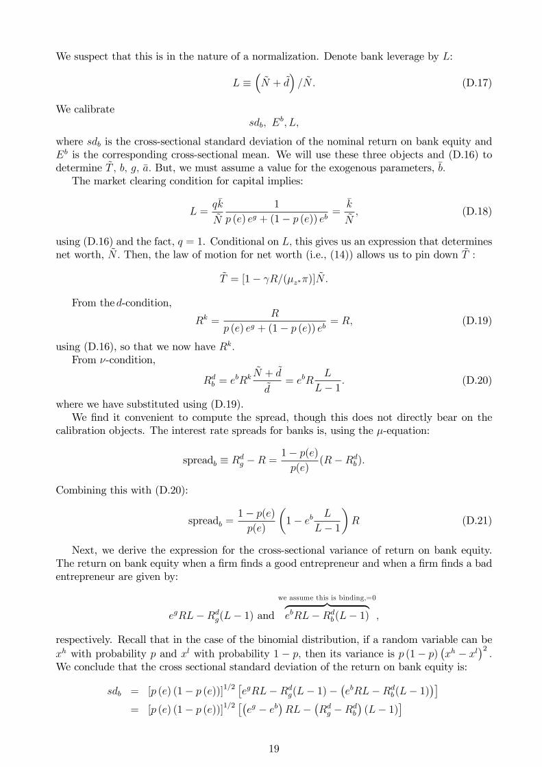
We suspect that this is in the nature of a normalization. Denote bank leverage by L:

L ≡(N + d

)/N. (D.17)

We calibratesdb, E

b, L,

where sdb is the cross-sectional standard deviation of the nominal return on bank equity andEb is the corresponding cross-sectional mean. We will use these three objects and (D.16) todetermine T , b, g, a. But, we must assume a value for the exogenous parameters, b.The market clearing condition for capital implies:

L =qk

N

1

p (e) eg + (1− p (e)) eb=

k

N, (D.18)

using (D.16) and the fact, q = 1. Conditional on L, this gives us an expression that determinesnet worth, N . Then, the law of motion for net worth (i.e., (14)) allows us to pin down T :

T = [1− γR/(µz∗π)]N .

From the d-condition,

Rk =R

p (e) eg + (1− p (e)) eb= R, (D.19)

using (D.16), so that we now have Rk.From ν-condition,

Rdb = ebRk N + d

d= ebR

L

L− 1. (D.20)

where we have substituted using (D.19).We find it convenient to compute the spread, though this does not directly bear on the

calibration objects. The interest rate spreads for banks is, using the µ-equation:

spreadb ≡ Rdg −R =

1− p(e)p(e)

(R−Rdb).

Combining this with (D.20):

spreadb =1− p(e)p(e)

(1− eb L

L− 1

)R (D.21)

Next, we derive the expression for the cross-sectional variance of return on bank equity.The return on bank equity when a firm finds a good entrepreneur and when a firm finds a badentrepreneur are given by:

egRL−Rdg(L− 1) and

we assume this is binding,=0︷ ︸︸ ︷ebRL−Rd

b(L− 1) ,

respectively. Recall that in the case of the binomial distribution, if a random variable can bexh with probability p and xl with probability 1 − p, then its variance is p (1− p)

(xh − xl

)2.

We conclude that the cross sectional standard deviation of the return on bank equity is:

sdb = [p (e) (1− p (e))]1/2[egRL−Rd

g(L− 1)−(ebRL−Rd

b(L− 1))]

= [p (e) (1− p (e))]1/2[(eg − eb

)RL−

(Rdg −Rd

b

)(L− 1)

]19

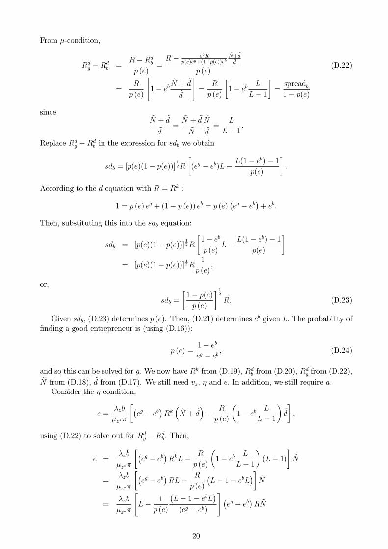
From µ-condition,

Rdg −Rd

b =R−Rd

b

p (e)=R− ebR

p(e)eg+(1−p(e))ebN+dd

p (e)(D.22)

=R

p (e)

[1− eb N + d

d

]=

R

p (e)

[1− eb L

L− 1

]=spreadb1− p(e)

sinceN + d

d=N + d

N

N

d=

L

L− 1.

Replace Rdg −Rd

b in the expression for sdb we obtain

sdb = [p(e)(1− p(e))] 12R[(eg − eb)L− L(1− eb)− 1

p(e)

].

According to the d equation with R = Rk :

1 = p (e) eg + (1− p (e)) eb = p (e)(eg − eb

)+ eb.

Then, substituting this into the sdb equation:

sdb = [p(e)(1− p(e))] 12R[

1− ebp (e)

L− L(1− eb)− 1

p(e)

]= [p(e)(1− p(e))] 12R 1

p (e),

or,

sdb =

[1− p(e)p (e)

] 12

R. (D.23)

Given sdb, (D.23) determines p (e). Then, (D.21) determines eb given L. The probability offinding a good entrepreneur is (using (D.16)):

p (e) =1− ebeg − eb , (D.24)

and so this can be solved for g.We now have Rk from (D.19), Rdb from (D.20), R

dg from (D.22),

N from (D.18), d from (D.17). We still need vz, η and e. In addition, we still require a.Consider the η-condition,

e =λz b

µz∗π

[(eg − eb

)Rk(N + d

)− R

p (e)

(1− eb L

L− 1

)d

],

using (D.22) to solve out for Rdg −Rd

b . Then,

e =λz b

µz∗π

[(eg − eb

)RkL− R

p (e)

(1− eb L

L− 1

)(L− 1)

]N

=λz b

µz∗π

[(eg − eb

)RL− R

p (e)

(L− 1− ebL

)]N

=λz b

µz∗π

[L− 1

p (e)

(L− 1− ebL

)(eg − eb)

] (eg − eb

)RN

20

Using (D.24),

e =λz b

µz∗π

[L− eg − eb

1− ebL(1− eb

)− 1

(eg − eb)

] (eg − eb

)RN

=λz b

µz∗π

[L−

L(1− eb

)− 1

1− eb

] (eg − eb

)RN

or,

e =λz b

µz∗π

eg − eb1− eb RN, (D.25)

which determines e. Next, we havep (e) = a+ be, (D.26)

which determines a.We still have the following two equations:

e : (λz + νz)1

µz∗πb(Rdg −Rd

b

)d+ η = 0, (D.27)

Rdg : νzp (e) + ηλz b = 0. (D.28)

Equations (D.27)-(D.28) are two equations in νz, η. Now solve for η using (D.27):

η = − (λz + νz)1

µz∗πb(Rdg −Rd

b

)d,

and use this to substitute out for η in (D.28):

νzp (e)− (λz + νz)1

µz∗πb(Rdg −Rd

b

)dλz b = 0,

or,

νz =

λzµz∗π

(b)2 (

Rdg −Rd

b

)dλz

p (e)− 1µz∗π

(b)2 (

Rdg −Rd

b

)dλz

(D.29)

η = − (λz + νz)1

µz∗πb(Rdg −Rd

b

)d. (D.30)

This completes the computations we set out to accomplish.

D.4 Steady State Algorithm, Unobserved Effort Equilibrium

Here is an algorithm. We specify a value for π and compute R using (D.9). From (D.19) weobtain Rk. From (D.11) we obtain rk. From (D.6) we obtain h/k. Solve (D.14) for w.Combining (D.12) and (D.13):

c+ g +i

µΥ

=

(k

hµ∗zΥ

)αh

1

λf.

Substituting out for i using (D.8) and dividing the result by h :

c

h+g

h+

(1− (1− δ) 1

µ∗zΥ

)kh

µΥ

=

(k

hµ∗zΥ

)α1

λf.

21

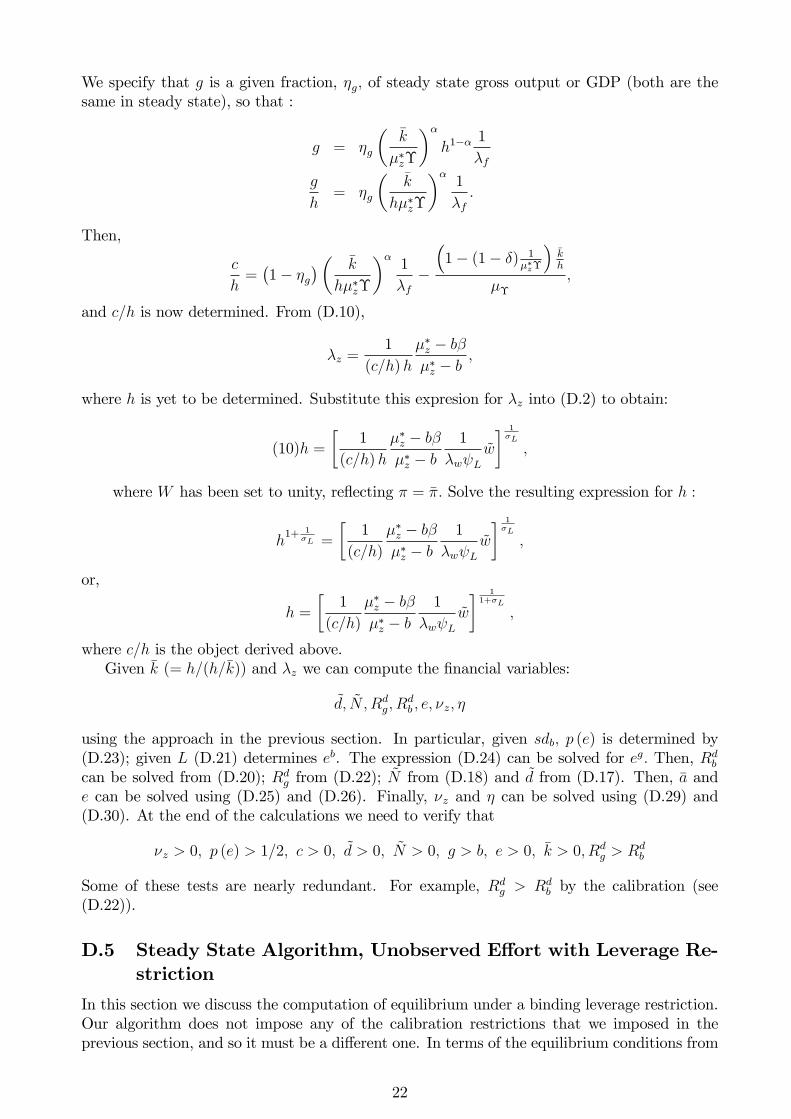
We specify that g is a given fraction, ηg, of steady state gross output or GDP (both are thesame in steady state), so that :

g = ηg

(k

µ∗zΥ

)αh1−α 1

λf

g

h= ηg

(k

hµ∗zΥ

)α1

λf.

Then,

c

h=(1− ηg

)( k

hµ∗zΥ

)α1

λf−

(1− (1− δ) 1

µ∗zΥ

)kh

µΥ

,

and c/h is now determined. From (D.10),

λz =1

(c/h)h

µ∗z − bβµ∗z − b

,

where h is yet to be determined. Substitute this expresion for λz into (D.2) to obtain:

(10)h =

[1

(c/h)h

µ∗z − bβµ∗z − b

1

λwψLw

] 1σL

,

where W has been set to unity, reflecting π = π. Solve the resulting expression for h :

h1+ 1

σL =

[1

(c/h)

µ∗z − bβµ∗z − b

1

λwψLw

] 1σL

,

or,

h =

[1

(c/h)

µ∗z − bβµ∗z − b

1

λwψLw

] 11+σL

,

where c/h is the object derived above.Given k (= h/(h/k)) and λz we can compute the financial variables:

d, N , Rdg, R

db , e, νz, η

using the approach in the previous section. In particular, given sdb, p (e) is determined by(D.23); given L (D.21) determines eb. The expression (D.24) can be solved for eg. Then, Rd

b

can be solved from (D.20); Rdg from (D.22); N from (D.18) and d from (D.17). Then, a and

e can be solved using (D.25) and (D.26). Finally, νz and η can be solved using (D.29) and(D.30). At the end of the calculations we need to verify that

νz > 0, p (e) > 1/2, c > 0, d > 0, N > 0, g > b, e > 0, k > 0, Rdg > Rd

b

Some of these tests are nearly redundant. For example, Rdg > Rd

b by the calibration (see(D.22)).

D.5 Steady State Algorithm, Unobserved Effort with Leverage Re-striction

In this section we discuss the computation of equilibrium under a binding leverage restriction.Our algorithm does not impose any of the calibration restrictions that we imposed in theprevious section, and so it must be a different one. In terms of the equilibrium conditions from

22

the section on price and wage equations, we have the equations in (D.5), which we reproducehere:

(1)s = 1/λf ,

(2)w = λwψLh

σL

λz.

In terms of the non-price and wage equations, we have (D.6) and (D.7):

(3)rk = α

(Υµ∗zh

k

)1−α

s,

(4)i =

[1

p (e) eg + (1− p (e)) eb− (1− δ) 1

µ∗zΥ

]k

We also have (D.9) and (D.10):

(5)R =πµ∗zβ,

(6)λz =1

c

µ∗z − bβµ∗z − b

.

The other equations listed right after this are:

s, w, h, λz, rk, k, i, e, R,Rk

(7)Rk =rk + 1− δ

Υπ

(8)c+ g +i

µΥ

=

(k

µ∗zΥ

)αh1−α − φ

Here, φ and g are exogenous parameters. They are not calibrated in this section.

(9)w = s (1− α)

[Υµz∗h

k

]−α.

23

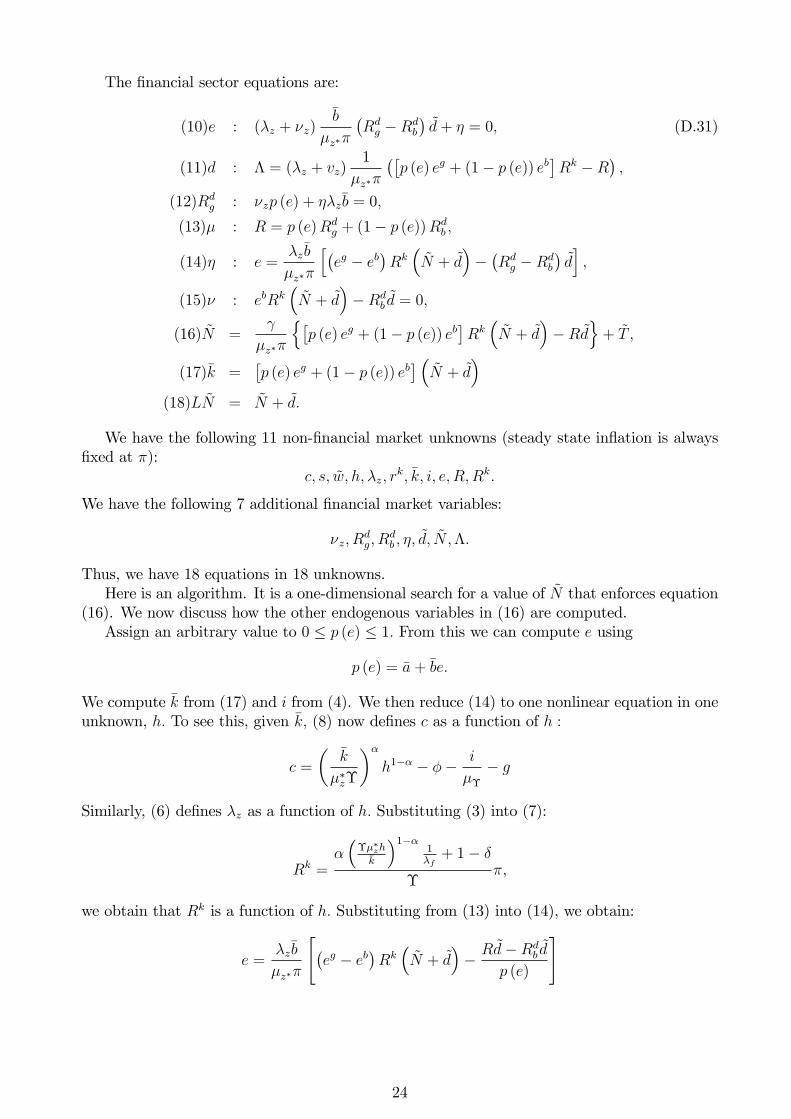
The financial sector equations are:

(10)e : (λz + νz)b

µz∗π

(Rdg −Rd

b

)d+ η = 0, (D.31)

(11)d : Λ = (λz + vz)1

µz∗π

([p (e) eg + (1− p (e)) eb

]Rk −R

),

(12)Rdg : νzp (e) + ηλz b = 0,

(13)µ : R = p (e)Rdg + (1− p (e))Rd

b ,

(14)η : e =λz b

µz∗π

[(eg − eb

)Rk(N + d

)−(Rdg −Rd

b

)d],

(15)ν : ebRk(N + d

)−Rd

b d = 0,

(16)N =γ

µz∗π

{[p (e) eg + (1− p (e)) eb

]Rk(N + d

)−Rd

}+ T ,

(17)k =[p (e) eg + (1− p (e)) eb

] (N + d

)(18)LN = N + d.

We have the following 11 non-financial market unknowns (steady state inflation is alwaysfixed at π):

c, s, w, h, λz, rk, k, i, e, R,Rk.

We have the following 7 additional financial market variables:

νz, Rdg, R

db , η, d, N ,Λ.

Thus, we have 18 equations in 18 unknowns.Here is an algorithm. It is a one-dimensional search for a value of N that enforces equation

(16). We now discuss how the other endogenous variables in (16) are computed.Assign an arbitrary value to 0 ≤ p (e) ≤ 1. From this we can compute e using

p (e) = a+ be.

We compute k from (17) and i from (4). We then reduce (14) to one nonlinear equation in oneunknown, h. To see this, given k, (8) now defines c as a function of h :

c =

(k

µ∗zΥ

)αh1−α − φ− i

µΥ

− g

Similarly, (6) defines λz as a function of h. Substituting (3) into (7):

Rk =α(

Υµ∗zhk

)1−α1λf

+ 1− δΥ

π,

we obtain that Rk is a function of h. Substituting from (13) into (14), we obtain:

e =λz b

µz∗π

[(eg − eb

)Rk(N + d

)− Rd−Rd

b d

p (e)

]

24

Substituting from (15):

e =λz b

µz∗π

(eg − eb)Rk(N + d

)−Rd− ebRk

(N + d

)p (e)

Note that the right hand side of this expression is a function of h alone. We adjust the valueof h until this expression is satisfied.We use (15) to compute

Rdb = ebRk N + d

d.

We also have Rdg from (13):

Rdg =

R− (1− p (e))Rdb

p (e).

We compute Λ from (11).Solving for η from (10):

η = − (λz + νz)b

µz∗π

(Rdg −Rd

b

)d.

Substitute this into (12)

νzp (e)− (λz + νz)b

µz∗π

(Rdg −Rd

b

)dλz b = 0,

and solving this for νz, we obtain:

νz =λz

bµz∗π

(Rdg −Rd

b

)dλz b

p (e)− bµz∗π

(Rdg −Rd

b

)dλz b

.

So that we have η and νz.Finally, we solve (9) for w. We adjust p (e) until (2) is satisfied. Thus, for an arbitrary

choice of value for N we compute p (e) and h as described above. We adjust the value of Nuntil (16) is satisfied.

D.6 Steady State Algorithm, Observed Effort

In the observed effort case, the equilibrium conditions for the financial sector do not requirecomputing Rd

g and Rdb and the multipliers, η and vz, are both zero. This means that we

can ignore equations (10), (12), (13), (15) in (D.31). Thus, the financial sector equilibriumconditions in nonstochastic steady state are:

25

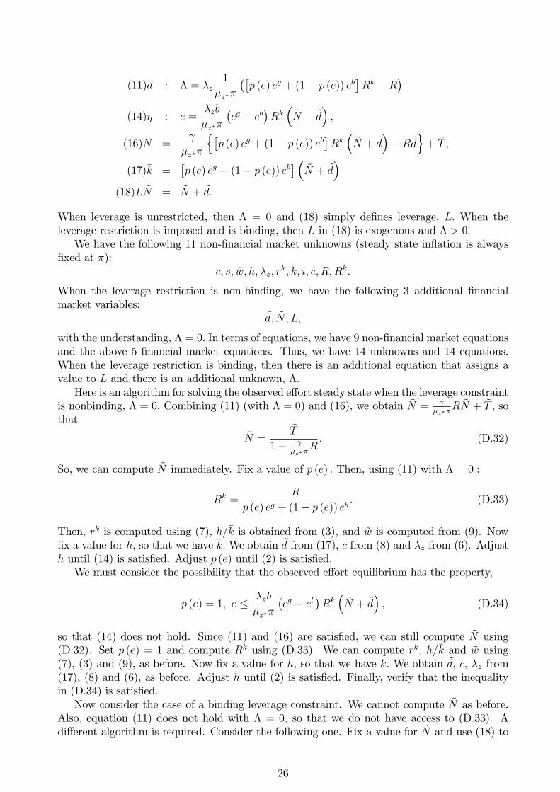
(11)d : Λ = λz1

µz∗π

([p (e) eg + (1− p (e)) eb

]Rk −R

)(14)η : e =

λz b

µz∗π

(eg − eb

)Rk(N + d

),

(16)N =γ

µz∗π

{[p (e) eg + (1− p (e)) eb

]Rk(N + d

)−Rd

}+ T ,

(17)k =[p (e) eg + (1− p (e)) eb

] (N + d

)(18)LN = N + d.

When leverage is unrestricted, then Λ = 0 and (18) simply defines leverage, L. When theleverage restriction is imposed and is binding, then L in (18) is exogenous and Λ > 0.We have the following 11 non-financial market unknowns (steady state inflation is always

fixed at π):c, s, w, h, λz, r

k, k, i, e, R,Rk.

When the leverage restriction is non-binding, we have the following 3 additional financialmarket variables:

d, N , L,

with the understanding, Λ = 0. In terms of equations, we have 9 non-financial market equationsand the above 5 financial market equations. Thus, we have 14 unknowns and 14 equations.When the leverage restriction is binding, then there is an additional equation that assigns avalue to L and there is an additional unknown, Λ.Here is an algorithm for solving the observed effort steady state when the leverage constraint

is nonbinding, Λ = 0. Combining (11) (with Λ = 0) and (16), we obtain N = γµz∗π

RN + T , sothat

N =T

1− γµz∗π

R. (D.32)

So, we can compute N immediately. Fix a value of p (e) . Then, using (11) with Λ = 0 :

Rk =R

p (e) eg + (1− p (e)) eb. (D.33)

Then, rk is computed using (7), h/k is obtained from (3), and w is computed from (9). Nowfix a value for h, so that we have k.We obtain d from (17), c from (8) and λz from (6). Adjusth until (14) is satisfied. Adjust p (e) until (2) is satisfied.We must consider the possibility that the observed effort equilibrium has the property,

p (e) = 1, e ≤ λz b

µz∗π

(eg − eb

)Rk(N + d

), (D.34)

so that (14) does not hold. Since (11) and (16) are satisfied, we can still compute N using(D.32). Set p (e) = 1 and compute Rk using (D.33). We can compute rk, h/k and w using(7), (3) and (9), as before. Now fix a value for h, so that we have k. We obtain d, c, λz from(17), (8) and (6), as before. Adjust h until (2) is satisfied. Finally, verify that the inequalityin (D.34) is satisfied.Now consider the case of a binding leverage constraint. We cannot compute N as before.

Also, equation (11) does not hold with Λ = 0, so that we do not have access to (D.33). Adifferent algorithm is required. Consider the following one. Fix a value for N and use (18) to

26

compute d. Fix p (e) . Use (17) to compute k. Use (4) to compute i.Fix h. Compute c from (8) and λz from (6). Compute rk from (3) and Rk from (7). Adjust

h until (14) is satisfied. Compute w from (9). Adjust p (e) until (2) is satisfied. Finally, adjustN until (16) is satisfied.Again, we must consider the possibility that p (e) = 1 and (14) does not hold. As before,

fix a value for N and use (18) to compute d. Set p (e) = 1 and compute k, i using (17) and (4).Fix a value for h. Compute c, λz, rk, Rk, w from (8), (6), (3), (7), (9). Adjust h until (2) issatisfied. Adjust N until (16) is satisfied. Finally, we must verify (D.34).

27