Leverage and Uncertainty

Mihail Turlakov1

Abstract

Risk and uncertainty will always be a matter of experience, luck, skills, and modelling.

Leverage is another concept, which is critical for the investor’s decisions and results. Adaptive

skills and quantitative probabilistic methods need to be used in successful management of risk,

uncertainty and leverage. The author explores how uncertainty beyond risk determines

consistent leverage in a simple model of the world with fat tails due to significant, not fully

quantifiable and not too rare events. Among particular technical results, for the single asset

fractional Kelly criterion is derived in the presence of the fat tails associated with subjective

uncertainty. For the multi-asset portfolio, Kelly criterion provides an insightful perspective on

Risk Parity strategies, which can be extended for the assets with fat tails.

1 Head of CVA desk, Global Markets division, Sberbank CIB. Mihail has about 10 years’ experience in financial industry in credit, FX and quantitative trading areas. He has worked on developing new business areas, modelling and trading while at RBS, Deutsche, WestLB and Sberbank. Before moving on to a financial career, Mihail worked as a researcher at the Departments of Physics in Cambridge and Oxford Universities in United Kingdom. He received his Ph.D. in theoretical condensed matter physics from University of Illinois at Urbana-Champaign in United States in 2000.

Uncertainty and risk play fundamental role in the portfolio and risk management. The more

objective measurable and the more subjective non-quantitative aspects of decisions can be

separated into risk and uncertainty correspondingly (Knight 1964). The risk, with known and

quantifiable probabilities and outcomes, became associated with the standard deviation (or

volatility) within classical expected utility theory and Black-Scholes-Merton theory. Not

surprisingly, the uncertainty is associated with other less understood, yet important, concepts

of unquantifiable outcomes, liquidity, partial information and subjective behavioural biases

(Booth 2014). Uncertainty and risk constrain the leverage (allocation size), which would

amplify the premium returns in unlimited way. While Kelly criterion (Kelly 1956) proposed

optimal leverage in the presence of risk, the fascinating conceptual link between leverage and

uncertainty is explored quantitatively and phenomenologically here.

General consequences of Kelly criterion in the world with fat tails are discussed with the

practical angle of the portfolio and risk management practitioner. In the view of the

complexity of modelling the processes and phenomena with fat (heavy or power-law) tails,

only a simple probabilistic model is analysed quantitatively here. The paper is organised as

follows. The introductory section “Risk and Uncertainty” sets the stage and discusses different

aspects of risk and uncertainty. The section “Risk and Leverage” reviews the conceptual links

between risk and leverage in the modern finance and introduces the Kelly criterion. The two

sections “Kelly criterion in the fat tails world” and “Kelly Parity” are more technical and

mathematical; these sections contain several novel quantitative results about Kelly criterion for

a single asset and for multi-asset portfolio calculated in a simple toy probabilistic model of the

world with fat tails. How the uncertainty, parametrised by left and right tails of the probability

distribution, changes the Kelly criterion is presented in the section “Kelly criterion in the fat

tails world”. Basic important connections are established between Kelly Parity, based on Kelly

criterion, Risk Parity, a popular risk control portfolio approach, and classic Mean-Variance

Optimization in the section “Kelly Parity”. The effects of the volatility skew and convexity2 on

Kelly Parity and Risk Parity are also discussed. The “Adaptive management of risk,

uncertainty, and leverage” section considers practical application of statistical Kelly system in

dynamic and intermittent real-world financial markets. The “Conclusion” section consolidates

the general insights and presents the outlook. Simple conceptual consequences of the

drawdown aversion, related to the uncertainty of the significant losses, on the efficient frontier

in the classic portfolio theory are explored in the appendix “Concave Efficient Frontier”.

Another appendix contains the details of Kelly criterion calculations in the simple probabilistic

model with a tail loss.

Risk and Uncertainty The key concepts of risk and uncertainty have been explored from different perspectives and

play different roles in any real life decision making. The risk is about quantifiable probabilities

and outcomes; the uncertainty is about degree of belief and subjectivity. From one side,

classical and neo-classical theoretical economics made tremendous progress by focusing on

risk in the framework of the probabilistic decision theory and the utility theory. Black-Scholes-

Merton theory (Black 1973) and Mean-Variance optimisation theory (Markowitz 1959) have

been developed in the rigorous mathematical formulation where the volatility represents the

risk. From another side, the practical finance and risk-management practices proceeded by

2 The volatility skew and convexity mean linear and quadratic adjustments as a function of the underlying asset. Equivalently, the (sufficiently large) volatility skew and volatility convexity (smile) in the Black-Scholes based description mean asymmetric left and right fat tails of the probability density function.

realising the duality3 between risk and uncertainty and defining the VaR boundary separating

them (Brown 2012). The inefficiency of the markets (Shiller 2005) and the behavioural biases

and aversions (Kahneman 1979) have been also recognized in driving the uncertainty of the

markets. Markets are uncertain as much as risky.

The uncertainty has many subjective and non-quantifiable, in the sense of Keynes and Knight,

aspects. The uncertainty can be associated with fat tails of the probability distributions.

Although this is certainly an oversimplification, I will make the following proposition; the risk

and the uncertainty can be associated with the centre and the fat tails of the probability density

functions (pdf’s) correspondingly. In this paper, I use this simple proposition, which allows

advancing the understanding of the uncertainty. Formally, under a unit measure, (the total

probability is one), the tails is what remains after the possible risks are quantified. In each

present moment, the price is clearly certain within bid and offer prices for any, unless very

illiquid, asset. The markets are more certain about the centre of the distribution, while the

investors differ in their subjective views more strongly about the tail outcomes4. To expand on

the above proposition, subjective probability distribution functions can be thought to be

incorporating all those subjective factors (limited information, behavioural biases, liquidity

information, limited capital, etc.) into the tails of the distribution functions of the individual

investors. Yet the centre of the distributions is quite constrained for all investors by the current

market valuations and “current markets consensus”. Subjective view on the risk can definitely

be different from the collective market view, but collective markets efficiency imposes strong

constraints at not too long time horizons. At longer time horizons and larger deviations5, the

uncertainty becomes more important, and notwithstanding the markets efficiency, the markets

are much more time dependent and inconsistent than the current pricing (of the forward curves

and the options at different maturities) suggests. Essentially, by their construction and their

actions, the markets explore and “quantify” the central “phase space”6 of possible risks7, and

the remote parts of the phase space represent the uncertainty. These remote parts of the pdf,

which have lower probability and longer time8 to be reached, are naturally assigned to the tails.

Several other aspects of the uncertainty are notable. Firstly, the subjective difference between

the price and the value is another definition of the uncertainty. At the height of panic or

irrational exuberance, the uncertainty as well as the mispricing are at the highest. Risk

perception may differ from risk reality, and the uncertainty is in the eye of the beholder.

Secondly, the uncertainty has a systemic component, due to the collective financial system,

and the idiosyncratic components due to unpredictable events (political, social, technological,

etc.). Thirdly, although many possible unpredictable events and their unstable sequences may

3 interconnectedness and complementarity 4 In particular, at-the-money and shorter-dated options are more liquid, while out-of-the money and/or longer-dated options are less liquid and have wider bid-offer spreads. 5 The delineating time horizon between the risk and the uncertainty seem to depend on the type of uncertainty itself. 6 The phase space (conventionally used in physics and other sciences) means the full space of all relevant variables of the system. 7 The fluctuations of the markets, due to news flow and all other factors, test the views and the positions of the investors; this process reveals the balance of “local risks”. Perhaps, in other words, the risk (volatility) are “local risks”, and the uncertainty is “remote risks”. 8 The property of markets to trend signifies the adaptability and confluence of various market mechanisms and participants (capital flows, leveraging, regulatory pressures, typical behaviour, etc.). Markets is a complex and non-ergodic system beyond simple physical systems, which explore the phase space progressively and ergodically.

occur, all these uncertainties need to be codified and lumped together into the fat tails. In other

words, the markets are clearly incomplete in the tails.

In reality, risk and uncertainty mix and not clearly delineated, while they might only be

separated in a graphical representation of pdf (probability density function) or any kind of a

model. The modelling of uncertainty is paradoxical, and the models are only metaphors, which

should not be taken too seriously (Derman 2012). After all, markets would not be needed if a

perfect (deterministic or stochastic) model existed, and the markets is efficient mechanism,

which is as of now “the worst, except for all others”. The related phenomena of subjectivity,

diversity and uncertainty appear to be essential and intrinsic for the competitive markets.

Several general points illustrate further the dichotomy and complementarity of risk and

uncertainty. Firstly, the diversification, one of the pillars of modern finance theory, is proposed

to reduce the ‘risks’9, yet the financial ‘risks’ do not disappear, but they transform into different

shapes and forms. To put it differently, the diversification rebalances the ‘risks’ between the

“familiar risk” around the centre of the distribution (the volatility) and the “uncertain risk”

of the tails of the distribution (the uncertainty). Secondly, a single realization of the future

possibilities carries enormous importance for the investors behaviourally, sociologically

(Nelson 2014) and organizationally (in the sense of agent-agency problem). The history is a

single path, not “Monte-Carlo averaged”10. The finite sample of important investor’s decisions

is ever present in mixing risk and uncertainty11, although the expected utility theory does not

distinguish between a single and multiple bets decisions (Samuelson 1963). Thirdly, in the

absence of the model12, the centre and the tails cannot be separated unambiguously, since the

volatility of the markets is time-dependent. For example, “Bayesian adjustment” in GARCH

models corrects what would be a naïve mixing of uncertainty and risk (Arnott 2005).

The mathematical description of the various real-life risks and the uncertainty is hard and

illusive, and in any case the high level of skill and experience is required in the application of

the quantitative models successfully in the real financial markets. It seems fair to say that,

although the empirical presence of fat tails in financial time series is widely accepted, there is

no well-established and accepted dynamic theory in finance13, which describes realistically the

fat tails. Major advances ( (Mandelbrot 1997), (Sornette 2004), (Engle 1995), (Mantegna

2000)) have been made to describe fat-tailed distributions, but there are principal and

conceptual differences between the markets and natural sciences. The limitations are non-

repeatability of history and the adaptability of the financial markets to name a few. Modelling

of outlier events can be problematic, as a matter of principle, and the models have to be used

sceptically. The quantitative models tend to be recalibrated on the new market data and lack

the predictive power of the models in the natural sciences. Yet, even in the absence of

scientifically sound dynamic models, the fat tails are the definitive manifestations of the

transitive dynamic reality and behavioural tendencies of the markets, and these innate

9 For no better word, ‘risks’ are used here and below only in the very general sense of the word. ‘Risks’ mean both the risk and the uncertainty of (Knight 1964) together without differentiating between them. 10 In finance, many future expectations are calculated by averaging over multiple future outcomes generated by Monte-Carlo method. 11 Quoting from “Risk and Uncertainty” of (Samuelson 1963): “… there will necessarily be left an epsilon of uncertainty even in so-called risk situations. As Gertrude Stein never said: Epsilon ain’t zero. This virtual remark has great importance for the attempt to create a difference of kind between risk and uncertainty in the economics of investment and decision making.” 12 For an important theoretical example, in the mathematical language, the binomial and Gaussian models possess only risk and none of uncertainty. 13 Some models in physics are phenomenological, but, arguably, the most powerful theories in physics are necessarily dynamic.

properties must be considered in any portfolio management quantitatively and qualitatively,

just like in the modern options pricing and management.

The fat-tailed nature of the distributions in finance is all-important and inherent, rather than

minor or secondary, property of the markets (Mandelbrot and Taleb 2010). “What risk really

means” is the very important question, and I think that uncertainty and possibility of a loss

associated with the downside fat tails is the most relevant threat. “What they fear is the

possibility of permanent loss” (Marks 2015). Thus, the risk management of the uncertainty and

fat tails is of critical importance. A recent model-free analysis of historical data showed that

for majority of the trading strategies (with several specific exceptions) the risk premium is

largely due to the presence of the skew or equivalently downside fat tail (Lemperiere 2015).

This major empirical finding14 incentivises deeper research into the connections between the

uncertainty (fat tails) and the leverage (capital allocation), which is the topic of this paper.

Leverage and Risk The leverage - the allocation size - is as important as the odds (the probabilities) of the

outcomes for the capital allocation decisions. The leverage needs to be decided in absolute

terms with respect to the investor’s available capital and in relative terms with respect to

relative allocation between different assets (or trading strategies) within the investor’s

portfolio. In the modern portfolio theory (Markowitz 1959), the relative allocation between

different assets, based on their expected returns, volatilities and correlations, is the focus of the

theory. The leverage financing of the modern financial system permits an investor to choose

the absolute leverage among other risk preferences. Leverage aversion changes the predictions

of the portfolio theory (Assness 2012), and modern Risk Parity (RP) strategies exploit this

opportunity. Leverage is a mechanism and a tool, not a danger in itself, while uncertainty and

permanent loss can definitely be associated with danger.

Absolute leverage is a risk decision determined by internal and external (due to the perception

of the counterparties providing leverage financing) factors. Uncertainty, rather than risk,

appears to be a more determining factor for the absolute leverage, since both, absolute leverage

and uncertainty, are more collectively determined properties with individual variations.

Qualitatively, uncertainty appears to be more important determinant of the absolute leverage,

risk determines relative leverages. The collective effects of aggregate market liquidity and

leverage have been elucidated (Adrian 2010) by pointing out the role of financial intermediaries

and credit cycles. Liquidity and uncertainty are complex and different for different market

participants. Market liquidity, funding liquidity (Brunnermeier 2008), absolute and relative

leverage, and uncertainty are intimately linked by direct and indirect mechanisms, and are very

much parts of the markets dynamics and challenges. Overall, the uncertainty and the liquidity

shed light on each other15. Both concepts are hard to define fully even qualitatively, and both

are complex and multi-dimensional16.

After the above overview of general aspects of the leverage, I would like to introduce the

mathematical Kelly criterion (Kelly 1956), which prescribes the optimal allocation of the

current capital for the ‘best long run’. Suppose a favourable outcome wins b units for every 14 The skew nature of risk premium appears to be more naturally sustainable by the markets unlike axiomatic risk premium, defined as volatility, of classical Capital Asset Pricing Model (CAPM). 15 For instance, low uncertainty suggests using higher leverage, and, just as well, high liquidity permits higher leverage in the trading. 16 Yet the past risk, in the sense of the volatility, can be calculated as the historical standard deviation of the past time series as well as future risk (future volatility) is traded and forecatsed by the options markets.

unit wager. Further, suppose that for each trial the win probability is p > 0, the lose probability

is q, and the expectation of the game pb-q >0 is positive. From optimization of the geometric

growth rate, the optimal fraction of the current capital is 𝑓∗ = (𝑏𝑝 − 𝑞)/𝑏. In the continuous

limit of the random Gaussian process with the expected return and the volatility 𝜎, Kelly

allocation is a dimensionless fraction 17 of the available capital 𝑓∗ = 𝜇/𝜎2 . The optimal

geometric growth rate is equal to 𝑔∗ =1

2𝜇𝑓∗. The quantitative and statistical power of Kelly

system rests on accurate estimate of the risk parameters and multiple bets “averaging”.

In the Gaussian (and binomial) model, in the absence of uncertainty (tails), the optimal leverage

is fully determined by the risk (the volatility) in the optimization problem for a given return.

For the binomial outcomes, the optimal allocation has several nice properties (Thorp 2006); (a)

maximizing the geometric growth rate, (b) minimizing the probability of ruin, (c) the penalty

in reduced growth rate for moderate underbetting, which offers a margin of safety, is not severe.

The drawbacks of Kelly system are as follows: (a) the intermediate returns are volatile roller

coasters (due to a constant proportion betting), (b) the drawdowns can be large, and (c) ruin is

possible. The practical application has also several challenges (M. J. Mauboussin 2006): (a)

the performance of money managers is frequently evaluated on arithmetic returns, not

geometric returns essential in Kelly system, (b) possible large drawdowns and loss aversion

can bias investors away from Kelly system.

Kelly criterion in the fat tails world Kelly criterion is a major theoretical insight, which provides a practical guideline, but the

application requires certainly adept skills and experience (Thorp 2006). In order to make

mathematical progress to extend Kelly criterion to the world with the uncertainty, we will have

to parametrise the tails of the pdf. Due to the theories of Savage and others, subjective

probabilities can be reduced to mathematical probabilities, although not always fully

consistently (Ellsberg 1961). The section “Adaptive management of risk, uncertainty, and

leverage” will discuss the practical aspects of the application of the extended Kelly criterion,

given the conceptual differences between uncertainty and quantifiable risk, in the real world.

Our aim in this section is to develop Kelly criterion in risky and uncertain world18 in the

presence of fat tails. The main quantity of the interest is the total wealth (capital) after many

(N) rounds of the financial bets 𝑊 = ∏ (1 + 𝑓𝑖 𝑋𝑖𝑁𝑖=1 ), where 𝑓𝑖 is the fraction of the capital

invested in the round 𝑖, and the (negative or positive) outcome is 𝑋𝑖. The problem is to find the

optimal fractions 𝑓𝑖 in order to maximize the final wealth and to minimize the unfavourable

outcomes and risks.

In the presence of the tail losses of the probability 𝛼 and the size 𝐸𝑇𝐿 and tail wins of the

probability 𝛽 and the size 𝐸𝑇𝑊, the generalized results for the leverage 𝑓1∗ and the growth

rate 𝑔1∗ of a single asset in a simple toy model are

17 Kelly fraction 𝜇/𝜎2 is a more natural and dimensionless risk-adjusted measure than Sharpe ratio 𝜇/𝜎, which depends on the time scale. In other words, the risk is the variance, more appropriately than the volatility (where the risk factor is being proportional to the volatility in CAPM). See also (Arnott 2005). 18 ‘Risky world’ means the world with the risk (the volatility), while ‘risky and uncertain world’ means the world of the volatility and fat tails. These worlds can be also called “Mediocristan” and “Extremistan” (Thorp, Mizusawa 2013).

𝑓1∗ ≈

𝜇

𝜎2

1 +𝛽 ∙ 𝐸𝑇𝑊 − 𝛼 ∙ 𝐸𝑇𝐿

𝜇 (1 − 𝛼 − 𝛽)

1 +𝛽 ∙ 𝐸𝑇𝑊2 + 𝛼 ∙ 𝐸𝑇𝐿2

𝜎2(1 − 𝛼 − 𝛽)

𝑔1∗ ≈ 0.5(1 − 𝛼 − 𝛽)

𝜇2

𝜎2

(1 +𝛽 ∙ 𝐸𝑇𝑊 − 𝛼 ∙ 𝐸𝑇𝐿

𝜇 (1 − 𝛼 − 𝛽))

2

1 +𝛽 ∙ 𝐸𝑇𝑊2 + 𝛼 ∙ 𝐸𝑇𝐿2

𝜎2(1 − 𝛼 − 𝛽)

The constant fraction betting is assumed, and the calculations are given in Appendix A. In the

case of 𝛽 ∙ 𝐸𝑇𝑊 = 𝛼 ∙ 𝐸𝑇𝐿, the volatility convexity, which results in the symmetric fat tails,

decreases the growth factor in two ways. First way is the multiplier (1 − 𝛼 − 𝛽), which is a

mere consequence of the probability weights taken away from the centre to the tails. Second

way is the multiplier 1 (1 +𝛽∙𝐸𝑇𝑊2+𝛼∙𝐸𝑇𝐿2

𝜎2(1−𝛼−𝛽)⁄ ), due to larger variance associated with the tails.

The remaining effect additional to the convexity effect is the skew effect (the volatility skew)

on the growth factor due to the multiplier (1 +𝛽∙𝐸𝑇𝑊−𝛼∙𝐸𝑇𝐿

𝜇 (1−𝛼−𝛽))

2

. For the simplicity, in the

absence of the right tail the skew effect of the fatter loss tail shows up as a correction (1 −2𝛼𝐸𝑇𝐿

𝜇(1−𝛼)) in the leading order of the 𝐸𝑇𝐿 parameter. Thus, the convexity and the downside (𝐸𝑇𝐿

related) skew reduce simple Kelly fraction 𝑓0∗ and the growth rate 𝑔0

∗. These results19 provide

a more detailed understanding why fractional Kelly ratio 𝑓1∗ must be used in practice (Thorp

2006). The important difference from Kelly criterion in risky world is that the tail parameters

𝛼, 𝐸𝑇𝐿, 𝛽, 𝐸𝑇𝑊 are subjective, and therefore the expectations about the growth rate 𝑔1∗ can

differ widely among different investors.

The uncertainty means that no model can express the parameters of the tails accurately;

nevertheless, the above results show that there are several qualitative fractional effects due to

the weight shift 𝛼 to the tails and due to the tail loss 𝐸𝑇𝐿. All effects are significant (of order

of fraction of unity), while the tail impact parameter 2𝛼𝐸𝑇𝐿

𝜇(1−𝛼) can easily make the growth rate

negative and therefore uncertain for the realistic parameters20. The chosen pdf function is a toy

model, which nevertheless gives important qualitative insights, while the realistic power-law

pdf would have to be investigated numerically. Although an asset may or may not have a

sufficiently skewed right tail for high positive capital growth, the non-linear payoffs of the

derivatives can have a right-tail skew. (Thorp, Mizusawa 2013) investigated in detail the capital

growth of the vanilla call options aiming to maximize the geometric returns with limited

drawdowns21. In the world of fat tails (“Extremistan”), they found that options portfolio attains

better regions of the geometric growth frontier than the underlying asset and have still better

profile of the drawdowns.

19 It is also clear that the leverage and growth rate can have so called convexity adjustments due the volatility of the volatility. 20 For instance, 𝛼 = 20%, 𝐸𝑇𝐿 = 30% and 𝜇 = 6%. 21 The wealth is a random multiplicative process, which is dominated by the most probable value in the finite sample rather than its “true average value” (Redner 1990). The crossover to the asymptotic “true average” growth of the product of N independent random numbers in the sampling is exponentially slow in N, and the impact of tail loss on the crossover and on the dominance of Kelly strategy are challenging issues. The path-dependent results should surely depend on the loss size ETL, and this is why the management of the drawdowns (limiting the losses) is critical.

The intuitive and tutorial understanding of the power of the geometric growth and the pitfalls

of the additional extreme outcomes is illustrated by a simple numerical example22. A run of

100 even bets (1 and -1 outcomes) with 60 winning bets and 40 losing bets is offered. Kelly

prescribes betting each time 20% of the current capital, which is the winning edge difference

between winning and losing. After 100 bankrolls, the optimal betting will give the “average

geometric return” of 749%. For a realistic sequence of only 100 bets, several “extreme sub-

sequences” will dominate; see below for the discussion of the statistics of the multiplicative

processes. Now suppose large losses or wins can happen. We can calculate the growth rate in

three more cases; Tail Loss (TL) for one bet out of 100 of losing three times your bet, Tail Win

(TW) for one bet out of 100 of winning three times your bet, Both Tails (BT) for one bet each

of winning and losing 3 times your bet. The growth rates are correspondingly𝑔𝑇𝐿 = 366%,

𝑔𝑇𝑊 = 1246% and 𝑔𝐵𝑇 = 545%. The variations of the growth rates are large, because the

optimal Kelly bet is highly sensitive to large tail wins and losses as well as to numerical effects

when the parameters of original losses/wins and tail losses/wins are comparable.

Kelly system provided key guidelines (M. J. Mauboussin 2006) for the practitioners in spite of

some objections from the mainstream economists. The mainstream economics focused on

developing probabilistic ensemble-average utility theory. Recent breakthrough understanding

(Peters 2011) of the differences between ensemble-average and time-average formulations

presents Kelly criterion in a new light and proposes the dynamic approach to the gamble

problem. The non-ergodic multiplicative processes can simulate the market dynamics and the

fat-tailed distributions, and the time-average formulation might provide better insights into the

dynamic leverage strategies beyond the optimization calculus of Kelly criterion23.

Kelly Parity In this section, I discuss how Kelly criterion applies to the multi-asset portfolio in the world

with or without fat tails. Important relations and differences between different portfolio

approaches of Mean-Variance (MV) optimization, based on classical MPT, Risk Parity (RP)

and Kelly Parity (KP) (to be defined below) emerge. Risk Parity is a risk-adjusted portfolio

management approach, which goes beyond the leverage aversion of conventional MPT

(Assness 2012). The most naïve RP approach is to allocate each asset in the Risk Parity

portfolio according to the risk-adjusted weight 1 𝜎𝑖⁄ , inversely proportionally to the asset’s

volatility 𝜎𝑖. A portfolio approach, which uses Kelly criterion for its construction, can be called

Kelly Parity. At the level of the definitions, Risk Parity pares assets based on their risks (usually

understood as the volatilities), while Kelly Parity pares assets based on their growth rates.

Kelly criterion in risky world gives the following allocation 𝑓𝑖 for the asset i of the N-asset

portfolio (Thorp 2006)

𝑓𝑖 = ∑ 𝐶𝑖𝑗−1𝑀𝑗 ,

𝑁

𝑗=1

22 See pages 175-176 of (Brown 2012). I modified slightly the example, since the case of initial 20% probability edge combined with one-sided possibility of 5-fold gains leads to the growth divergence. 23 In our analysis of Kelly criterion throughout the technical part of the paper, we assume that the risk premium and the fat tails are unrelated, in the future research it will be interesting to examine the risk premium being due to the fat tails in the context of the recent empirical finding (Lemperiere 2015)

where 𝐶𝑖𝑗−1 is the inverse matrix of the covariance matrix 𝐶𝑖𝑗 = 𝜌𝑖,𝑗𝜎𝑖𝜎𝑗 , and 𝑀𝑗 is the risk

premium vector. Kelly Parity prescribes allocations for all assets with the total portfolio

leverage 𝑍 = 1̅ ∗ 𝐶−1 ∗ 𝑀. In practice, there are constraints on specific and total leverage24,

and therefore a finite selection of the assets has to be made.

In the framework of MPT and MV optimization, the maximization of Sharpe Ratio =

𝑓𝑇𝑀 (𝑓𝑇 ∗ 𝐶 ∗ 𝑓)1

2⁄⁄ , subject to the constraint𝑓𝑇 ∗ 1̅ = 1, has to be done. Remarkably, the

solution (for instance, see (Chan 2008)) is equivalent to the Kelly solution with the absolute

leverage equal to one. This simple, not widely known, result is worth noting. Namely, Kelly

Parity prescribes not only the optimal absolute portfolio leverage but also relative leverages

of the assets identically to the mean-variance optimization (Markowitz 1959). Kelly Parity25

not only maximizes the long-term growth but also minimizes the variance for a given return

(by the virtue of the Sharpe ratio minimization).

Risk Parity and Mean Variance portfolio approaches are generally viewed to be different by

the construction. Risk Parity optimizes the variance without any reference to the expected risk

premiums, which are generally less predictable than the average volatilities, while Mean

Variance optimizes the Sharpe ratio in the space of the expected returns and the variances. It

appears that RP has “extreme parameter ignorance” in the sense of ignoring the input of the

expected returns26. Kelly Parity suggests a new perspective and a deeper connection between

RP and MV. Without going into the dependencies on correlations27, and, for the simplicity in

the limit of zero correlations, Kelly Parity is equivalent to Risk Parity if all assets have the

same Sharpe ratios. Kelly allocation 𝑓𝑖 = 𝜇𝑖 𝜎𝑖2⁄ becomes equivalent to the simple 𝑓𝑖 = 𝑆𝑅 𝜎𝑖⁄ ,

where Sharpe ratio factor is the same for all assets 𝑆𝑅 = 𝜇𝑖 𝜎𝑖⁄ . Sharpe ratio factor is the overall

leverage scaling remaining in RP approach to target particular return level. In fact, it can be

argued that RP makes implicit assumption of assets having equal Sharpe ratios in the efficient

markets, since from the beginning the focus of RP is on the balancing the assets by their

corresponding risks28.

Risk Parity encompasses a whole family of the strategies and implementations by building on

the sound idea of risk-adjusted allocation. Tail Risk Parity (Alankar 2012) is a radical

rethinking of RP, when the risk is defined as Expected Tail Loss, similar to the tail loss 𝐸𝑇𝐿 discussed above. TRP aims to control the tail risks without over-constraining the local variance

risks. In contrast, Mean-Variance optimization minimizes variance for a given level of return29,

but the minimization of the variance leads to increasing the large risks (fattening the tails)

(Sornette, Andersen and Simonetti 2000). Kelly growth calculations are insightful and practical

because the risk premium and tail risks can be treated in a balanced way.

24 Specific expressions for the one and two assets cases are given here. In the case of one asset, 𝑍 =

𝜇𝜎2⁄ is

exactly Kelly leverage. In the case of the two assets, for instance, the first asset has absolute leverage 𝑍1 =

(𝜇1 𝜎12⁄ − 𝜌 𝜇2 (𝜎1𝜎2)⁄ ) (1 − 𝜌2)⁄ , relative leverage is 𝑍1 𝑍⁄ , where the total leverage is 𝑍 =

(𝜇1 𝜎12⁄ + 𝜇2 𝜎2

2⁄ − 𝜌(𝜇1 + 𝜇2) (𝜎1𝜎2)⁄ ) (1 − 𝜌2)⁄ .

25 in risky world but not necessarily in risky and uncertain world 26 In other words, RP is agnostic about the expected returns. 27 This technical point can be investigated separately in the future. 28 We will not delve here into the practical application of Kelly Parity and Risk Parity based on the assets or factors (Bhansali V. 2012) and practical successes of RP due to secular trends and structural reasons. 29 In some constructions, Risk Parity determines the relative allocation of the assets in the portfolio by leveraging them to the same return.

The close connections between all three different portfolio approaches (MV, RP and KP) show

that Kelly Parity is on the solid ground for the portfolio construction ‘in the risky world’. More

challenging to investigate next is how Kelly Parity can be extended for skewed and convex

assets. In what follows, we generalize how individual skews and convexities of each asset add

up or balance each other in Kelly Parity of multi-asset portfolio in risky and uncertain world.

Our next task is to elucidate qualitative aspects of the skew and convexity effects at the simple

conceptual level of Risk Parity and Kelly Parity portfolio approaches30, while the technical

mathematical analysis for the multi-asset portfolio with power-law tailed assets have been

attempted before (for instance, (Bouchard, et al. 1998)). In the simplest case if assets are

uncorrelated, the rescaling of the leverage is independent. Nevertheless some assets, previously

selected to the most optimal portfolio, can become less attractive and upended by other assets

due to the different suppression of the growth rates by downside fat tails. More generally, we

can consider two correlated or anti-correlated assets. The two assets can have the skews co-

aligned or anti-aligned with the assets correlation. For instance, skew co-alignment means that

the implied and realized volatilities increase for both assets in their typical correlated move. In

terms of the toy model explored in this paper, skew co-alignment means that both assets are

correlated not only occurring in their normal volatility states simultaneously but also in their

corresponding tail loss states. The full technical details will need to be presented in a separate

future paper, and the portfolio solutions can depend in complex ways on parameters. Analytical

results can be viewed as tail loss perturbation corrections to Kelly Parity portfolios in terms of

small parameters 𝛼 𝐸𝑇𝐿

𝜇,

𝛼 𝐸𝑇𝐿2

𝜎2 and 𝜇 𝐸𝑇𝐿

𝜎2 . Numerical results can also be calculated for the

realistic probability density functions. In simple cases, natural results can be expected with

further suppression of the growth rate in the case correlated co-aligned skews; for instance, the

factor 𝛼 ∙ 𝐸𝑇𝐿1 is replaced by 𝛼 ∙ 𝐸𝑇𝐿1(1 + 𝜇2𝐸𝑇𝐿2 𝜎22).⁄ More interesting case is anti-

correlated assets with skew alignment, in this case the absolute leverage and growth rate may

not be suppressed noticeably. How a multi-asset portfolio can be optimised relative to (several)

possible extreme scenarios is a separate interesting problem, which is similar to Tail Risk Parity

(Alankar 2012). Multi-asset portfolio choice and optimization can aim to balance

simultaneously the diversification in the few scenarios of the tail events and the amplification

of the growth rate at the normal volatility core.

Adaptive management of risk, uncertainty and leverage Active Risk Management (RM) can embrace the complex interplay between risk, uncertainty,

and leverage guided by the quantitative principles. Human decision making with its

behavioural aspects need to be brought together with the quantitative insights in the overall

RM framework. After all, human decisions and adaptability remain central to the financial

markets and portfolio management, at least at the current, still quite basic, stage of the artificial

intelligence and the quantitative understanding of the complex systems, markets and

economics.

Fear, greed and some rationality drive the financial markets and the financial decision-making.

In the prospect theory, (Kahneman 1979) underlined the choice value “… assigned to gains

and losses rather than to final assets and in which probabilities are replaced by decision

30 Another interesting direction of the research is how the trend strategy can be combined with Risk Parity and Kelly Parity and hedge their skews and convexity. The trend strategy is positive convexity (Bouchard, et al. 2016) and positive skew, while Kelly Parity and Risk Parity in their simplest forms are naturally negative skew and positive convexity.

weights.” The certainty is preferred to the uncertainty; moreover, the individuals tend to be risk

averse in the face of gains and risk seeking in the face of losses. The uncertainty of fear

dominates the uncertainty of greed; this asymmetry sustains a negative skew of equity markets.

All markets have symmetric or asymmetric fat tails expressed in the volatility skew and

convexity. Furthermore, Ellsberg paradox (Ellsberg 1961) illustrates how the uncertainty and

the complexity reduce the risk appetite. The financial decision-making has to recognise how

the behavioural views on the uncertainty feeds into the quantitative choice of leverage.

The drawdown aversion can express the fear of the permanent loss. The drawdown, defined as

a certain percentage loss of the capital, is a natural and important risk measure from the

prospect theory perspective, and the associated aversion to the drawdown has to be managed

accordingly with behavioural individual preferences. The conventional MPT and CAPM,

dealing with the final assets, as per above quote, can only consider the drawdown aversion as

an afterthought (see the Appendix B). How the drawdown aversion, expressed through the

uncertainty of the tail loss, changes the single-asset allocation (Kelly leverage) and the multi-

asset portfolio theory, is one of the central topics of this paper. The drawdown aversion is

rational, quantified by fractional Kelly criterion for fat-tailed assets, and behavioural, and both

aspects are self-reinforcing.

In the absence of the tail risks, the leverage has to be scaled inversely with the variance (if the

risk premium remains fixed) during stable periods of the variance. Kelly system underlined

practical risk-management systems of several, if not many, successful practitioners. “The

natural risk” is the variance (Arnott 2005) (Kelly 1956), not the volatility. Kelly fraction is an

important dimensionless risk measure, which is different from the Sharpe ratio. “Thus the Kelly

investor will dynamically reallocate as optimal 𝑓∗ changes over time because of fluctuations

in the forecast…” (Thorp 2006) of the excess return and the volatility31. Even in the risky

world, the challenges are many from quantitative to behavioural. Among quantitative ones are

the evaluation of the risky parameters and the edge of the Kelly system showing up only slowly

in the number of the financial bets in the crossover from the most probable to the “true average”

(Redner 1990). The numerous behavioural ones (Peterson 2007) are the rational view on the

possible long drawdowns, not “taking profits too soon”, and other “path dependencies”. In the

world with the uncertainty tails, Kelly criterion is one of the guidelines for making decisions.

The range of the decisions can be narrowed, but not to an obviously optimal choice, since the

uncertainty is much less certain than the risk32. This is always the case in the real world as

Kelly criterion can rarely be used literally.

Risk taking and risk management are the art and the skills of making good and certain decisions

under uncertainty. The perceived uncertainty33 and the chosen leverage are the parts of the

various positive and negative feedback loops, which enforce the adaptation of the collective

markets and the individual investors to new information and new strategies. The interaction of

adaptive investor and adaptive markets34 is the dynamic capital allocation game.

The risk management regimes can be classified into the three regions by the magnitude of the

market downside fluctuations, i. e. relative losses (consistently with the prospect theory). The

normal volatility region (“white swans”) is around the centre of pdf within -10%. The

31 The fluctuations of the volatility (volatility of volatility) and the fluctuations of the tail parameters (tail probability and tail loss) can produce so-called convexity adjustments. 32 However obvious or tautological this statement is. 33 The evaluation of the uncertainty and the risks is one of the main behavioural and rational tasks. 34 The important problem is how single-agent strategy is consistent with the multi-agent system representing the markets. A consistency of multi-agent beliefs and risk views with their interactions is far beyond this paper.

transitional area between -10% and -25% can be called “grey swans”, the precursors to “black

swans”. Lastly, the “black swans” (Taleb 2008) region of the tail beyond -25% moves. Each

region requires different operational modes of the decisions and actions (Bhansali 2014) in

terms of active portfolio management. Diversification and dynamic rebalancing are appropriate

risk-management approaches in the normal volatility region. The transitional region is of the

pivotal importance35, connecting the normal region with the fully unpredictable region of

“black swans”, and this is where the uncertainties and risks are most finely balanced. The

experience, the transitional hedging strategies (the options and momentum strategies are

particularly pertinent), and the adaptive rational decisions can make huge difference. “Grey

swans” is the key region, where the risk manager’s behaviour, the risk judgement and the

quantitative framework become complementary. Since the “black swan” region is extremely

rare and defined as completely unpredictable, then the best way to think about “black swans”

is to take considerate care of “grey swans”.

Risk-management system is a behavioural and quantitative framework, which embodies “a

talent of managing events as they arise”. The risk-management system has to protect the

competitive edge36 from deep or unrecoverable setbacks. One of the main consequences of the

uncertainty, made clear by Kelly calculations, is very familiar; do not underestimate the

uncertainty, do not overleverage. The hedging of tail risk (Bhansali 2014) is a necessity not a

luxury. Even diversified portfolio has some systemic and concentration risks from the threat of

some particular events. Different assets and hedges have not only different instrinsic (relative

to capital structure, i.e. equity or debt) but also payoff and instrument based (options, CDS,

etc.) convexity and skew, and these non-linear effects are critical in the management of grey

swans. The portfolio of different financial assets (equity, debt, etc.) and instruments (OTC

derivatives, futures, ETFs, etc.) have to be scrutinized for sufficient market and funding

liqudity when liquidity can be hard to obtain. The uncertainty of dangers and opportunities

(Brown 2012) requires proxy hedging and imaginative approaches. Tail hedging is an asset-

allocation decision, and different mentality, organisational setup and behavioural biases of

managing the core portfolio versus the tail risk hedging can benefit the overall portfolio.

“Edge is the key” is the main principle of risk taking. In the world of the quantifiable risk,

Kelly criterion builds on the amplification of the risk premium (edge) through the leverage.

Maximizing the long-term multi-period37 growth rate and minimizing the ruin chances is

exactly how Kelly criterion strikes the fine balance and makes the edge effective. In the great

debate about the advantages and disadvantages of the active and passive management, the

skilful management of leverage and uncertainty is where the active management can lead by

exploiting the leverage and the professional judgement about uncertainty.

Due to the intermittent nature of the markets, successful management of leverage and

uncertainty have to be path-dependent and adaptive. The origin of risk premiums is critical for

the appropriate investor strategy, although the risk premium (the edge) is assumed a priori in

the Kelly calculations. Different cases of risk premiums and uncertainty require specialised

35 In the note of caution from the famous investor, Peter Lynch: “Far more money has been lost by investors preparing for corrections, or trying to anticipate corrections, than has been lost in corrections themselves”. 36 In the Kelly calculations in this paper, the edge is assumed to be around the centre of pdf, which is a good description only for certain businesses (credit institutions, high-yield funds, etc.). 37 In practice, for many different reasons, multiple-periods reinvestment with stable quantifiable edge is rarely possible. The volatility (noise), the uncertainty and the competitive deterioration of any edge are very powerful drivers of the markets, which make the sustainability of the edge very difficult and very rare.

firms and different adaptive strategies38. The basic balance of greed and fear can be seen

already from simple expressions of the toy model for the arithmetic growth factor 𝑟 =(1 − 𝛼)𝜇 − 𝛼 ∙ 𝐸𝑇𝐿 in the presence of however small probability 𝛼 of a tail loss. Although

the greed of the risk premium (1 − 𝛼)𝜇 can exceed the expected losses of the fear 𝛼 ∙ 𝐸𝑇𝐿, a

onetime loss 𝐸𝑇𝐿 can be significant. The investors attempt to outsmart each other by banking

on greed gains and trying to avoid the fear losses. Important sequence of the good outcomes in

the finite sample (relative to market odds in the probabilistic sense) by luck and skill is not

underestimated by many investors in comparison with the statistical long-run edge, and this

observation creates important dynamics of the markets. The markets do permit relatively stable

risk premiums and volatility regimes over some time periods, which can be exploited by

statistical Thorp-Kelly systems, but regime changes have to be recognized by the outside

adaptable decision maker.

Taking advantage of the diversity breakdowns (M. Mauboussin 2007) (regime changes) and

benefiting from the expected value mindset (M. Mauboussin 2004) take us into the heart of the

realistic and successful management of grey swans. “Dramatic diversity breakdown” and “time

arbitrage breakdown” are important market heuristics of the regime changes, which are

characteristic of the complex adaptive systems. Diversity breakdowns become triggered as

more and more investors recognize particular patterns (viewed as trends or risk premiums),

initiated at different times and managed to different time horizons, and deploy higher leverage

under collectively perceived and diminishing uncertainty. Subjective views become less

diverse resulting in the diversity breakdowns. Risk premium strategies, which can be levered

according to Kelly criterion, appear to compete with the diversity breakdowns, which spark

sharp or even violent trends. In any case, open competition of the investors‘ strategies in the

allocation of capital makes good markets. Another aspect is that liquidity has to be

commensurate with the leverage and the investor strategy. Liquidity is a very important part of

the feedback loops, where the investor provides and depends on the liquidity from the complex

markets. In practice, risk taking not only can be empowered by the statistical quantitative

methods (like Kelly criterion) but also has to evolve by adapting to the regime changes and the

diversity and liquidity breakdowns.

Uncertainty and leverage are the key risk preferences. Prices (information and patterns),

preferences (aversions, uncertainty, and leverage), and probabilities (risk) have been

highlighted to encompass consistent risk management (Lo 1999). Risk taking and management

are about consilience of qualitative, quantitative, technical and behavioural skills, which come

together, in particular, in the judgement about the uncertainty and choosing the leverage

accordingly. Risk management and risk taking are dual. The same events, the same grey swans,

bring dangers and opportunities associated with uncertainty. Interestingly, on general grounds,

in the entrepreneurial context (Knight 1964) thought that the uncertainty deserves much higher

returns than the risk. Consistent and skilful management of the uncertainty and the leverage

can be the source of structural edge, especially since the market risk premiums can be largely

due to the uncertainty (Lemperiere 2015).

38 Realistic markets also exhibit various memory and correlation effects in the risk and uncertainty pricing, and there is good value for risk takers in recognizing even the short-range correlations in multiplicative processes (see nice mathematical illustrations in (Redner 1990)). The pattern recognition is one of the salient properties of good risk takers; see for example, a classic book (Lefevre 2005).

Conclusion The leverage and the uncertainty have to be managed consistently in a proper, even though

subjective, risk-management framework, and several practical results and guidelines have been

discussed here. In particular, the uncertainty determines how fractional Kelly criterion can be

used more effectively in practice. The fractional weight can be estimated, not exactly

calculated, from the subjective probability weights and the severity of the uncertainty tails.

Uncertainty, due to many uncontrollable and unpredictable events, constraints leverage beyond

risk.

Kelly Parity, multi-asset portfolio based on Kelly criterion of optimisation of geometric growth

rates, encompasses major, widely known, portfolio approaches of Risk Parity and Mean-

Variance optimization. In particular, Kelly Parity becomes Mean-Variance Optimization if the

absolute leverage is constrained to unity. Kelly Parity becomes basic Risk Parity if the Sharpe

ratio of all involved assets is the same. Due to the volatility convexity and skew (parametrized

by left and right tails), Kelly Parity has to adjust absolute and relative leverages.

“The fundamental law of investing is the uncertainty of the future” (Bernstein 1992). The

management of leverage and uncertainty is one of the most important strands in successful

investing. The paper presents a certain perspective and a programme for the future empirical

and theoretical research with many open questions. Human decision-making, adaptiveness, and

the drawdown management are discussed phenomenologically from the practitioner’s

perspective. Adaptive and skilful management of uncertainty and leverage can build a

successful edge by taking on “grey swans” opportunities and managing possible drawdowns.

References

Adrian, T., Shin, H. S. “Liquidity and Leverage.” Journalof Financial Intermediation, 2010: v. 19 (3), p.

418-37.

Alankar, A., DePalma, M., Scholes, M. “The introduction into Tail Risk Parity.” preprint,

AlllianceBernstein research, 2012.

Arnott, Robert D. “What cost 'noise'?” Financial Analyst Journal, 2005: March/April: 10-14.

Assness, C., Frazzini, A., Pedersen, L. H. “Leverage Aversion and Risk Parity.” January/February 2012:

47-59.

Bernstein, Peter L. Capital Ideas. New York: Free Press, 1992.

Bhansali V., Davis J., Rennison, G., Hsu, J., Li, F. “The risk in Risk Parity - a factor-based analysis of

asset-based Risk Parity.” The Journal of Investing, 2012.

Bhansali, Vineer. Tail Risk Hedging. Creating robust portfolios for volatile markets. McGraw Hill

Education, 2014.

Black, F., Scholes, M. “The pricing of options and corporate liabilities.” Journal of Polictical Economy,

81, 1973: 637-659.

Booth, Jerome. Emerging Markets in an Upside Down World, Challenging Perceptions in Asset

Allocation and Investment. Wiley, 2014.

Bouchard, J. P., T. L. Dao, T. T. Nguyen, C. Deremble, Y. Lemperiere, and M. Potters. “Tail protection

forlong investors: trendconvexity at work.” preprint (to be published), 2016.

Bouchard, J.P., Sornette D., Walter C., and Aguilar J.P. “Taming large events: optimal portfolio theory

forstrongly fluctuating assets.” Int.Journal of Theoreticaland Applied Finance, 1998: 25-41.

Brown, Aaron. Red-blooded risk. The secret history of Wall Street. John Wiley & Sons, Inc., 2012.

Brunnermeier, M., Pedersen L. H. “Market Liquidity and Funding Liquidity.” 2008.

Chan, Ernie. Quantitative Trading: how to build your own algorithmic business. New Jersey: John

Wiley & Sons, 2008.

Derman, E. Models. Behaving. Badly.: Why Confusing Illusion with Reality Can Lead to Disaster, on

Wall Street and in Life. Wiley, 2012.

Ellsberg, D. “Risk, Ambiguity,and the Savage Axioms.” Quaterly J. Econ, 1961.

Engle, R. F. ARCH: selected readings. Oxford University Press, 1995.

Gregory, Jon. Counterparty credit risk and credit valuation adjustment. John Wiley & Sons, 2012.

Illinski, K., Pokrovski, A. “Lies of Capital Lines.” preprint by "Fusion Asset Management", 2010.

Kahneman, D., Tversky, A. “Prospect Theory: an analysis of decision under risk.” Econometrica 47(2),

1979: 263-291.

Kelly, J.L. “A new interpretation of information rate.” Bell Systems Technical Journal 35, 1956: 917-

926.

Knight, Frank H. Risk, Uncertainty and Profit. New York: Augustus M. Kelley, Bookseller, 1964.

Lefevre, E. Reminiscences of a stock operator. New Jersey: John Wiley & Sons, 2005.

Lemperiere, Y., C. Deremble, Trung-Tu Nguyen, Ph. Seager, M. Potters, J-P Bouchaud. “Tail risk

premiums versus pure alpha.” Risk magazine, risk.net ("Risk"magazine, RISK.NET), 2015.

Lo, Andrew W. “The Three P's of Total Risk Management.” Financial Analysts Journal, 1999.

Mandelbrot. Fractals and Scaling in Finance. Springer-Verlag, 1997.

Mandelbrot, B, and N. Taleb. “Mild vs Wild Randomness: Focusing on Those Risks That Matter.” The

Known, the Unknown, and the Unknowable in Financial Risk Management, 2010: 47-58.

Mantegna, R. N., Stanley H. E. An introduction to Econophysics: Correlations and Complexity in

Finance . Cambridge University Press, 2000.

Markowitz, H. Portfolio Selection. Wiley, 1959.

Marks, Howard. “Risk revisited again, June 2015.” Memo to Oaktree clients, 2015.

Mauboussin, M. The decision-making for investors. Theory, practice and the pitfalls. preprint, New

York: Legg Mason, 2004.

Mauboussin, M. The wisdom and whims of the collective. Legg Mason Capital Management, preprint,

2007.

Mauboussin, Michael J. “Size Matters.” preprint by Legg Mason Capital Management, 2006.

Nelson, S., Katzenstein, P. “Uncertainty, Risk, and the Financial Crisis of 2008.” International

Organization, 2014: 361-392.

Peters, O. “Optimal leverage from non-ergodicity.” Quant. Fin. 11, 2011: 1593-1602.

Peterson, Richard L. Inside the investor'sbrain. The power of mind over money. New Jersey: John

Wiley & Sons , 2007.

Redner, S. “Random multiplicative processes: an elementary tutorial.” Am. J. Phys. 58 (3), 1990: 267-

273.

Samuelson, P. “Risk and Uncertainty: a fallacy of large numbers.” Scientia, 1963.

Shiller, R. J. Irrational Exuberance. Princeton University Press, 2005.

Sornette, D. Why Stock Markets Crash: critical events in complex financial systems. Princeton

University Press, 2004.

Sornette, D., J. V. Andersen, and P. Simonetti. “Minimizing volatility increases large risks.” Int.J.

Theor. Appl. Finance, 2000: 523-535.

Taleb, N. N. The Black Swan. The impact of the highly improbable. London: Pinguin Group, 2008.

Thorp, E. “The Kelly criterion in blackjack sports betting, and the stock market.” Handbook of Asset

and Liability Management, edited by S. A. Zenios and W. Zemba, 2006: chapter 9.

Thorp, Mizusawa. “Maximizing Capital Growth with Black Swan Protection.” In Handbook of the

Fundamentals of Financial Decision Making, p. 15-28. 2013.

Appendix A. Analytical calculation for the pdf with the tail loss

probability. The original Kelly criterion can be reproduced by using a pdf as a sum of the two delta

functions. The pdf is of the form 𝑃(𝑥) = 0.5 (𝛿(𝜇 + 𝜎) + 𝛿(𝜇 − 𝜎)), where the excess return

𝜇 and the volatility 𝜎 are parameters. We assume the limit 𝜎 ≫ 𝜇 for the consistency with

Kelly calculations. The geometric growth rate (Thorp 2006) as a function of constant fraction

of the invested capital 𝑓 is

𝑔0(𝑓) = 0.5 ln(1 + 𝑓(𝜇 + 𝜎)) + 0.5 ln(1 + 𝑓(𝜇 − 𝜎)).

The maximization solution gives 𝑓0∗ =

𝜇

𝜎2−𝜇2≈

𝜇

𝜎2 and gives 𝑔0(𝑓0

∗) ≈ 0.5𝜇2

𝜎2 consistently

with the Thorp’s results.

A physical interpretation of Kelly leverage is the ratio of the diffusion time 1 𝜎2⁄ divided by the

drift time 1 𝜇⁄ . In this interpretation, small allocation 𝑓∗ ≪ 1 means that the drift time 1 𝜇⁄ is

longer than the diffusion time 1 𝜎2⁄ , and the “return edge” is small (the geometric growth

𝑔(𝑓∗) is smaller than the return 𝜇). High allocation 𝑓∗ ≫ 1 means that the growth is fast

enough, not eroded too quickly by the noise, in this case the drift time is shorter than the

diffusion time.

We would like to analyze the results in the case of possible, but rare, large tail losses. The pdf

can be defined as 𝑃(𝑦) = 𝛼 𝛿(𝑦 + 𝐸𝑇𝐿) +1−𝛼

2[δ(y − (μ + σ)) + δ(y − (μ − σ))], where the

additional parameters are the probability of the tail loss 𝛼 and the size of the tail loss 𝐸𝑇𝐿

(Expected Tail Loss). For the same “positive edge”, the condition 𝜇 > 𝛼 ∙ 𝐸𝑇𝐿 is required. The

relation 𝜇0

𝜎02 <

1

𝐸𝑇𝐿 is required for the growth rate 𝑔(𝑓) staying well defined at the tail loss state.

The regime 1

𝐸𝑇𝐿<

1

𝜎 implies the tail loss is noticeably larger than the volatility.

The geometric growth function, to be maximized, is

𝑔(𝑓) = 𝛼 ln(1 − 𝑓 ∙ 𝐸𝑇𝐿) +1−𝛼

2[ln(1 + 𝑓(𝜇 + 𝜎)) + ln(1 + 𝑓(𝜇 − 𝜎))].

The relevant solution39 continuously connected with the original 𝑓∗ is40

𝑓1∗ ≈

𝜇 − 𝛼(𝜇 + 𝐸𝑇𝐿)

𝜎2 − 𝜇2 + 𝛼(2𝜇𝐸𝑇𝐿 − (𝜎2 − 𝜇2))≈

𝜇

𝜎2

(1 −𝛼𝐸𝑇𝐿

𝜇(1 − 𝛼))

(1 +𝛼𝐸𝑇𝐿2

𝜎2(1 − 𝛼))

𝑓1∗ is dependent on the tail loss 𝐸𝑇𝐿 in the two combinations

𝛼𝐸𝑇𝐿

𝜇(1−𝛼) and

𝛼𝐸𝑇𝐿2

𝜎2(1−𝛼). Clearly, 𝑓1

∗ <

𝑓∗ is reduced by numerical factor , and the growth rate is smaller as well

𝑔(𝑓1∗) ≈

𝜇2

2𝜎2(1 − 𝛼)

(1 −𝛼𝐸𝑇𝐿

𝜇(1 − 𝛼))

2

(1 +𝛼𝐸𝑇𝐿2

𝜎2(1 − 𝛼))

39 The model considered here is a static model based on the pdf. It would be interesting to generalize the model to the dynamic model and the limit of large N-steps (p.22 of (Thorp 2006)). The time scale related to the tail loss mixing and the scaling with N would be of interest. 40 Perhaps, some of these results are due to the particular form of the logarithm dependence. Notice that the exponential growth function is naturally logarithmic. The growth function is conceptually different from the conventional utility function of the probabilistic utility theory.

It is interesting that the effect of the relative impact parameter (1 −𝛼𝐸𝑇𝐿

𝜇(1−𝛼)) on the growth rate

𝑔(𝑓1∗) is only quadratic. We can see clearly41 that the growth rate decreases sharply when

2𝛼𝐸𝑇𝐿 becomes of the same order as the excess return 𝜇, this condition is more stringent by a

factor of 2 than the threshold for the positivity of the arithmetic growth rate (also the first

moment) −𝛼 ∙ 𝐸𝑇𝐿 + (1 − 𝛼)𝜇 > 0. This result illustrates the robustness of the Kelly system

to the perturbative tail effects, but the adjustment of the leverage is esssential nevertheless. A

dynamical model would shed more light on the different timescales associated with the drift,

diffusion, the tail loss and their mixing.

The above analytical results were tested by the exact numerical solution of the lengthy

quadratic equation for 𝑓1∗ . The parameters of the return and the volatility can be recalibrated

to the original parameters as follows. The mean and the variance are given by the expresions

< 𝑦 > = −𝛼 ∙ 𝐸𝑇𝐿 + (1 − 𝛼)𝜇 and < 𝑦2 > = 𝛼 ∙ 𝐸𝑇𝐿2 + (1 − 𝛼)(𝜇2 + 𝜎2). If the original

excess return 𝜇0 and the volatility 𝜎0 are substituted, then the calibrated values of 𝜇 and 𝜎 are

𝜇 =𝜇0

1−𝛼+

𝛼

1−𝛼𝐸𝑇𝐿 and 𝜎2 =

𝜎02

1−𝛼− 𝛼(𝐸𝑇𝐿 + 𝜇)2. One observation, which emerges from the

numerical parameter testing, is that the the growth rate can remain stable. At the same time,

the leverage needs to be increased significantly when 𝐸𝑇𝐿 increases. A qualitative

interpretation of this numerical finding is that the tail loss can remain hidden and unnoticed at

the level of average growth. But many path-dependent properties do change due to the tail loss

(for instance, the drawdown distribution), especially in the view of slow convergence of the

multiplicative process.

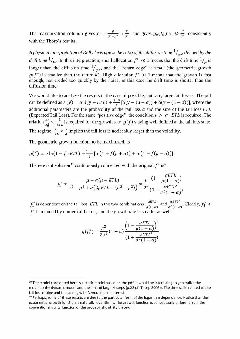
Another observation is that for sufficiently strong tail loss 𝐸𝑇𝐿 the solution 𝑓1∗ switches from

positive to negative smoothly. This means that for strongly skewed asset it is optimal to “short

the asset”. This result is shown in the Figure below.

41 The full set of the conditions is (a) ) 𝜎 ≫ 𝜇 for the consistency of the low leverage approximation of the

assumed pdf (b) 𝜇0

𝜎02 <

1

𝐸𝑇𝐿 to preserve the original maximum of the growth function (c) 𝛼 ≪ 1 for the

perturbative effect of the tail loss (d) 𝐸𝑇𝐿

𝜇> 1 for the meaningful parameter choice.

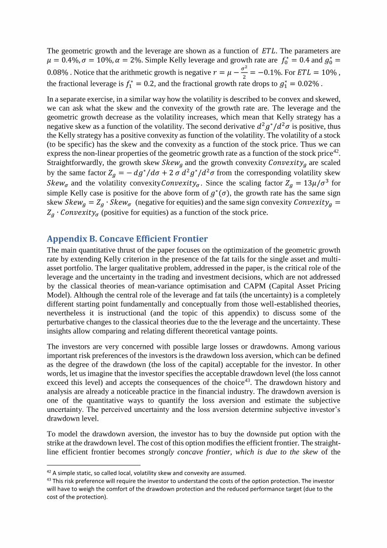
The geometric growth and the leverage are shown as a function of 𝐸𝑇𝐿. The parameters are

𝜇 = 0.4%, 𝜎 = 10%, 𝛼 = 2%. Simple Kelly leverage and growth rate are 𝑓0∗ = 0.4 and 𝑔0

∗ =

0.08% . Notice that the arithmetic growth is negative 𝑟 = 𝜇 −𝜎2

2= −0.1%. For 𝐸𝑇𝐿 = 10% ,

the fractional leverage is 𝑓1∗ = 0.2, and the fractional growth rate drops to 𝑔1

∗ = 0.02% .

In a separate exercise, in a similar way how the volatility is described to be convex and skewed,

we can ask what the skew and the convexity of the growth rate are. The leverage and the

geometric growth decrease as the volatility increases, which mean that Kelly strategy has a

negative skew as a function of the volatility. The second derivative 𝑑2𝑔∗/𝑑2𝜎 is positive, thus

the Kelly strategy has a positive convexity as function of the volatility. The volatility of a stock

(to be specific) has the skew and the convexity as a function of the stock price. Thus we can

express the non-linear properties of the geometric growth rate as a function of the stock price42.

Straightforwardly, the growth skew 𝑆𝑘𝑒𝑤𝑔 and the growth convexity 𝐶𝑜𝑛𝑣𝑒𝑥𝑖𝑡𝑦𝑔 are scaled

by the same factor 𝑍𝑔 = − 𝑑𝑔∗ 𝑑𝜎⁄ + 2 𝜎 𝑑2𝑔∗/𝑑2𝜎 from the corresponding volatility skew

𝑆𝑘𝑒𝑤𝜎 and the volatility convexity𝐶𝑜𝑛𝑣𝑒𝑥𝑖𝑡𝑦𝜎 . Since the scaling factor 𝑍𝑔 = 13𝜇/𝜎3 for

simple Kelly case is positive for the above form of 𝑔∗(𝜎), the growth rate has the same sign

skew 𝑆𝑘𝑒𝑤𝑔 = 𝑍𝑔 ∙ 𝑆𝑘𝑒𝑤𝜎 (negative for equities) and the same sign convexity 𝐶𝑜𝑛𝑣𝑒𝑥𝑖𝑡𝑦𝑔 =

𝑍𝑔 ∙ 𝐶𝑜𝑛𝑣𝑒𝑥𝑖𝑡𝑦𝜎 (positive for equities) as a function of the stock price.

Appendix B. Concave Efficient Frontier The main quantitative thrust of the paper focuses on the optimization of the geometric growth

rate by extending Kelly criterion in the presence of the fat tails for the single asset and multi-

asset portfolio. The larger qualitative problem, addressed in the paper, is the critical role of the

leverage and the uncertainty in the trading and investment decisions, which are not addressed

by the classical theories of mean-variance optimisation and CAPM (Capital Asset Pricing

Model). Although the central role of the leverage and fat tails (the uncertainty) is a completely

different starting point fundamentally and conceptually from those well-established theories,

nevertheless it is instructional (and the topic of this appendix) to discuss some of the

perturbative changes to the classical theories due to the the leverage and the uncertainty. These

insights allow comparing and relating different theoretical vantage points.

The investors are very concerned with possible large losses or drawdowns. Among various

important risk preferences of the investors is the drawdown loss aversion, which can be defined

as the degree of the drawdown (the loss of the capital) acceptable for the investor. In other

words, let us imagine that the investor specifies the acceptable drawdown level (the loss cannot

exceed this level) and accepts the consequences of the choice43. The drawdown history and

analysis are already a noticeable practice in the financial industry. The drawdown aversion is

one of the quantitative ways to quantify the loss aversion and estimate the subjective

uncertainty. The perceived uncertainty and the loss aversion determine subjective investor’s

drawdown level.

To model the drawdown aversion, the investor has to buy the downside put option with the

strike at the drawdown level. The cost of this option modifies the efficient frontier. The straight-

line efficient frontier becomes strongly concave frontier, which is due to the skew of the

42 A simple static, so called local, volatility skew and convexity are assumed. 43 This risk preference will require the investor to understand the costs of the option protection. The investor will have to weigh the comfort of the drawdown protection and the reduced performance target (due to the cost of the protection).

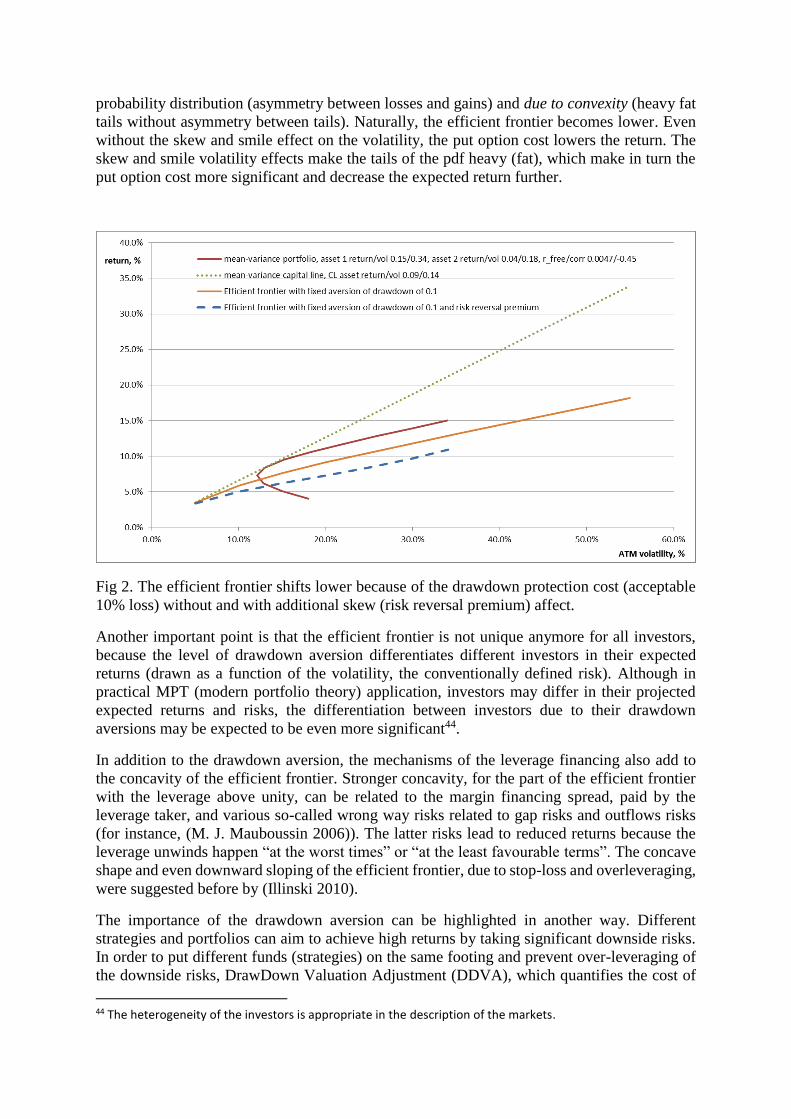
probability distribution (asymmetry between losses and gains) and due to convexity (heavy fat

tails without asymmetry between tails). Naturally, the efficient frontier becomes lower. Even

without the skew and smile effect on the volatility, the put option cost lowers the return. The

skew and smile volatility effects make the tails of the pdf heavy (fat), which make in turn the

put option cost more significant and decrease the expected return further.

Fig 2. The efficient frontier shifts lower because of the drawdown protection cost (acceptable

10% loss) without and with additional skew (risk reversal premium) affect.

Another important point is that the efficient frontier is not unique anymore for all investors,

because the level of drawdown aversion differentiates different investors in their expected

returns (drawn as a function of the volatility, the conventionally defined risk). Although in

practical MPT (modern portfolio theory) application, investors may differ in their projected

expected returns and risks, the differentiation between investors due to their drawdown

aversions may be expected to be even more significant44.

In addition to the drawdown aversion, the mechanisms of the leverage financing also add to

the concavity of the efficient frontier. Stronger concavity, for the part of the efficient frontier

with the leverage above unity, can be related to the margin financing spread, paid by the

leverage taker, and various so-called wrong way risks related to gap risks and outflows risks

(for instance, (M. J. Mauboussin 2006)). The latter risks lead to reduced returns because the

leverage unwinds happen “at the worst times” or “at the least favourable terms”. The concave

shape and even downward sloping of the efficient frontier, due to stop-loss and overleveraging,

were suggested before by (Illinski 2010).

The importance of the drawdown aversion can be highlighted in another way. Different

strategies and portfolios can aim to achieve high returns by taking significant downside risks.

In order to put different funds (strategies) on the same footing and prevent over-leveraging of

the downside risks, DrawDown Valuation Adjustment (DDVA), which quantifies the cost of

44 The heterogeneity of the investors is appropriate in the description of the markets.

the drawdown protection for a given drawdown level, can be introduced. This type of the

valuation adjustment is similar in spirit to the so called CVA (Credit Valuation Adjustment)

from the derivatives industry (Gregory 2012). CVA expresses a valuation adjustment to MtM

(Mark-to-Market) value of the derivatives due to the counterparty credit risk not mitigated by

any collateral. CVA eliminated the arbitrage between the cash instruments (bonds, etc.) and

the derivative instruments. Similarly, the Drawdown VA should eliminate the arbitrage

between the funds taking excessive risks in the sense of possible significant loss and the funds

taking more balanced risks. The conceptual difference between CVA and DDVA is that

Drawdown VA is proposed to be calculated below a certain drawdown strike, corresponding

to a certain level of loss. Thus a certain range of the volatility is not penalized. DDVA at

“certain loss level” is consistent with the main risk being “a permanent loss”, where the investor

cannot accept further losses beyond the drawdown level, while she accepts the volatility at the

“normal course of events”. Such an adjustment would be challenging the financial industry to

implement for many reasons, from technical to educational; nevertheless, this adjustment

reflects a realistic value adjustment due to loss uncertainties. In the context of MPT, Markowitz

stressed the applicability of the utility theory beyond Gaussian distributions, but he did not

consider explicitly the drawdown aversion and multi-period growth rate calculated by the Kelly

criterion.

In summary, by introducing DDVA adjustment due to the drawdown aversion within the

framework of MPT, we noticed that the risk premium on the efficient frontier (per unit of asset)

depends not only on the volatility (as in CAPM) but also non-linearly on the drawdown

aversion and the leverage. This conclusion highlights that there are non-linear feedback effects

between the investor’s choices of the leverage, the views on the uncertainty and the expected

returns.