Leverage and Beliefs:

Personal Experience and Risk Taking in Margin Lending*

Peter Koudijs+ Hans-Joachim Voth++

9 September 2015

Abstract: What determines risk-bearing capacity and the amount of leverage in financial markets? Using unique archival data on collateralized lending, we show that personal experience can affect individual risk-taking and aggregate leverage. When an investor syndicate speculating in Amsterdam in 1772 went bankrupt, many lenders were exposed. In the end, none of them actually lost money. Nonetheless, only those at risk of losing money changed their behavior markedly – they lent with much higher haircuts. The rest continued largely as before. The differential change is remarkable since the distress was public knowledge. Overall leverage in the Amsterdam stock market declined as a result.

JEL codes:

Keywords: Leverage, collateralized lending, haircuts, personal experience

* We thank seminar participants at Caltech, CREI Barcelona, Northwestern, Stanford, UC Berkeley, University of British Columbia, the NBER Corporate Finance meeting (Fall 2013), the SITE Asset Pricing meeting (Summer 2013), and the BGSE 2013 Summer Forum for feedback. We are grateful to Ran Abramitzky, Paul Beaudry, Effi Benmelech, Markus Brunnermeier, Vicente Cuñat, Ian Dew-Becker, Darrell Duffie, Patrick Francois, William Fuchs, Carola Frydman (discussant), Mariassunta Giannetti, Francisco Perez Gonzales, Gary Gorton (discussant), Filippo Ippolitto, Dirk Jenter, Gregor Matvos, Chris Meissner (discussant), Stefan Nagel, Marco Pagano, Luigi Pascali, Enrico Perrotti, Jose Luis Peydro, Giacomo Ponzetto, Josh Rauh, Michael Roberts, David Romer, Jean-Laurent Rosenthal, and Amit Seru for valuable comments and suggestions. Daphne Acoca, Tim Kooijmans, Dmitry Orlov, Inken Töwe and Victor Westrupp provided outstanding research assistance. All errors are our own. + Stanford GSB and NBER, koudijs@stanford.edu ++ University of Zurich, UBS Center and CEPR, voth@econ.uzh.ch

2

Leverage in financial markets is not constant over time. Lending is typically pro-cyclical –

high and increasing in good times, and much lower when asset prices fall (Adrian and Shin

2010). For example, when the stock market crashed after Lehman’s bankruptcy in 2008,

“haircuts”1 increased sharply and the volume of collateralized lending collapsed (Gorton and

Metrick 2012; Krishnamurthy, Nagel, and Orlov 2012). Pro-cyclical “leverage cycles” affect

the risk-bearing capacity of financial intermediaries and can contribute to large changes in

asset prices (He and Krishnamurthy 2013).2 The source of these important changes is less

clear.3

We argue that changes in beliefs on the part of lenders can explain shifts in market-

wide leverage, and that personal experience is an important determinant of these changes.

Our argument is related to a literature examining the effects of individual experience on

behavior in financial markets. Malmendier and Nagel (2011) demonstrate that individuals

who lived through the Great Depression invested systematically less in equities, even after

controlling for age, gender, and income. Guiso, Sapienza, and Zingales (2011) show that

during the recent financial crisis, Italian investors became markedly more risk averse. In an

experimental setting, inducing fear can lead to lower risk-taking (Cohn et al. 2015). Key

challenges in this literature are to show that changes in attitudes can affect aggregate risk-

bearing capacity, even in markets with sophisticated participants, and that changes in

behavior are not simply a reflection of lower wealth.4

In this paper, we show that adverse experiences can change beliefs, leading to large

increases in haircuts in a sophisticated and liquid loan market, creating pro-cyclical leverage

in the aggregate. Importantly, lenders’ personal willingness to take risks declined even

without individual losses. Using hand-collected data from notary archives, we focus on

margin loans in the 18th-century Amsterdam stock market. This setting has two key

advantages. First, loans were collateralized with securities that had readily observed market

prices, and leverage can easily be measured by the haircuts imposed. Second, because loan

1 The difference between the asset’s market value and the loan amount, the reciprocal of leverage. 2 Resulting changes in asset prices are observationally equivalent to changes in risk aversion, which contribute importantly to price swings in the aggregate (Campbell and Cochrane 1995; Cochrane 2011). 3 Regulatory and technical constraints – such as VAR limits –can help to rationalize large shifts in credit provided to financial markets (Adrian and Shin 2010; Geanakoplos 2010). Several contributions to the literature on pro-cyclical leverage argue that volatility of asset prices is greater in bad states of the world (Brunnermeier and Pedersen 2005; Vayanos 2004). Fostel and Geanakoplos (2008) rationalize this finding in a setting with heterogeneous agents. 4 Guiso, Sapienza and Zingales (2011) find no correlation with wealth, consumption patterns, or other sources of risk. Brunnermeier and Nagel (2008) conclude that wealth fluctuations only have minor effects on risk tolerance.

3

contracts were negotiated in an over-the-counter (OTC) market, we can identify the impact of

differences in lenders’ personal experience on the cross-section of haircuts. We focus on one

particular episode of financial distress around Christmas 1772. The Seppenwolde syndicate

speculated in East India Company stock. Lenders exposed to the syndicate were at risk of

significant financial losses, but escaped unharmed. Uncertainty was resolved within a matter

of weeks. Financiers who had lent to the syndicate before became more conservative. Before

the crisis, collateral requirements of exposed lenders were indistinguishable from the rest of

the market. Suddenly, after the Seppenwolde bankruptcy, lenders involved with the syndicate

only extended loans with markedly higher haircuts (Figure 1, Panel A). Their average “down

payment” rose from 20 to almost 30% within six months. Other lenders – not at risk of

personal losses – conducted business as usual.

Major lenders to the stricken syndicate changed their behavior, influencing aggregate

market conditions. The tightening of collateral requirements in the Amsterdam secured

lending market after Christmas 1772 is fully explained by former financiers of the syndicate

lending with higher haircuts. At the same time, interest rates on loans extended by both

groups of lenders remained unchanged (Figure 1, Panel B), and exposed lenders did not exit

the sample at a higher rate. Other margins of adjustment point towards lower risk-taking:

Affected lenders reduced their volume of margin lending overall and started to lend to less

risky borrowers. Importantly, although haircuts of exposed and non-exposed lenders

eventually began to converge (after a year), the effect remains visible for as long as we have

data – a one-off, large shock changed the behavior of major players substantially and for an

extended period.

Why did borrowers not simply shift towards lenders that were not affected by the

Seppenwolde bankruptcy? There was no centralized exchange for loans and borrowers had to

search for potential lenders. Who they matched with depended on who happened to have

liquidity available at the right moment. Our identification therefore relies on the accidental

timing of liquidity needs. After Christmas 1772, unaffected lenders were generally in short

supply; and borrowers had to settle for higher haircuts if their funding need happened to

coincide with available funds in the hands of an exposed lender. In other words, the

differential response of haircuts is observable because of the search-and-matching process

between lenders and borrowers. We rationalize these changes in an OTC market version of

Geanakoplos’ (2003) repo lending model, emphasizing investor heterogeneity. Optimists

borrow to buy a risky asset while pessimists lend. In equilibrium, speculation in risky

securities is financed by contracts involving minimal risk to the lenders; the cost of risky

4

contracts would be prohibitive from the perspective of the borrower.5 Fluctuations in haircuts

reflect changes in the level of disagreement between investors about the payoff of an asset or

shifts in investor characteristics, such as the share of optimists and pessimists.6 By only

affecting one set of investors – and their lenders – the distress in the Amsterdam stock market

in 1772/1773 increased lender heterogeneity. Having only narrowly escaped from losses,

affected lenders became more pessimistic; consistent with Geanakoplos (2003), they

demanded higher haircuts. In our historical setting, personal experience changed behavior,

generating pro-cyclical leverage in the aggregate.

We can rule out several alternative interpretations: Losses amongst intermediaries,

which may have played an important role in the recent crisis (Brunnermeier and Pedersen

2005; Adrian and Shin 2010), were unimportant.7 Also, the price fall was largely exogenous,

driven by the arrival of negative news about fundamentals in Bengal. Lenders at risk of losing

money then reduced the riskiness of their lending by raising collateral requirements. Despite

the decline in effective funding for speculators, the price decline was limited and reversed

quickly; no “loss spirals” followed the sharp shift in haircuts. Because lenders did not suffer

any losses, higher haircuts cannot reflect an increase in (wealth-dependent) risk aversion.

Finally, increases in haircuts were not driven by regulatory constraints, such as VAR limits,

which can drive fire sales (Brunnermeier and Pedersen 2009).

Our research contributes to the literature on asset prices and heterogeneous beliefs

more generally. Differences in beliefs can be important for asset pricing (Miller 1977;

Harrison and Kreps 1978; Jarrow 1980; Hong and Stein 2007). Where these differences come

from is an area of active research. Agents may have access to different information sets

(Brunnermeier 2001; Hong, Kubik, and Stein 2005a)8 or have different beliefs as a result of

their own experiences. The latter is often called reinforcement learning (Camerer and Ho

1999; Erev and Roth 1998). A number of contributions look at the impact of experience on

decision making in financial markets (Choi et al. 2009; Greenwood and Nagel 2009; Kaustia

5 In the Geanakoplos model, agents with more optimistic beliefs want to lever up to invest in the asset. Pessimistic agents do not want to hold the asset directly, but are willing to lend to the optimists on the collateral of the asset. The equilibrium contract turns out to be risk free. The haircut is set such that even in the worst possible state of the world lenders are fully repaid. From a borrower’s perspective it is prohibitively expensive to contract a risky loan with a lower haircut – he expects to always pay a high risk premium, even in states of the world where the more pessimistic lender expects him to default. 6 Simsek (2013) uses a Geanakoplos-style model to analyse the effects of more general types of disagreement. 7 For a historical example, cf. Schnabel and Shin (2004). 8 Social networks can shape investor attitudes (Hong, Kubik, and Stein 2005b) and attitudes more generally (Acemoglu and Jackson 2011); social capital can boost trust in the stock market (Guiso, Sapienza, and Zingales 2008a).

5

and Knüpfer 2008; and Vissing-Jorgenson 2003).9 Malmendier and Nagel (2011, 2013) show

that both the Great Depression and high inflation in the 1970s influenced expectations and

behavior. Guiso, Sapienza, and Zingales (2011) argue that experiencing a financial crisis can

induce a big change in risk appetite. In the same spirit, Heath and Tversky (1991) conclude

that the willingness to take risks declines sharply with distrust in one’s own judgement.

Murfin (2012) shows that banks impose stricter loan covenants when they suffer losses on

their loan portfolios. More generally, our work connects with research on the determinants of

attitudes and beliefs.10

Our paper also contributes to the literature using historical data on haircuts as a

measure of expectations. Rappoport and White (1994) argue that increasing margin

requirements in the run-up to the 1929 crash on the NYSE reflected growing worries about a

coming crash. Temin and Voth (2004) argue that haircuts in lending against stock during the

South Sea bubble suggest that investors were “riding” the bubble. Schnabel and Shin (2004)

argue that leverage cycles created contagion and falling asset prices in the Amsterdam

financial crisis of 1763 (Quinn and Roberds 2012).

We proceed as follows. Section I discusses the historical background. Section II

summarizes the key features of our model of secured lending. Section III describes the data.

Section IV presents the main empirical results, and section V considers a variety of

extensions and robustness checks. Section VI concludes. Additional material is in

Appendices A – G; references to figures and tables starting with a corresponding letter can be

found there.

I. Historical Background

We first describe the nature of collateralized lending in 18th century Amsterdam. We briefly

explain the East India Company’s situation, and summarize evidence on the investment

syndicate’s bankruptcy. Finally, we describe how the authorities dealt with the crisis.

I.A. Collateralized Lending in 18th century Amsterdam 

The market for secured lending in 18th century Amsterdam resembles the market for margin

loans in modern-day markets. It can be traced back to the early 17th century (Gelderblom and

9 A formal model of experience-based belief formation is Piketty (1995). 10 Malmendier and Tate (2007) and Graham and Narasimhan (2004) find that corporate managers who were born before the Great Depression make more conservative capital structure decisions. Malmendier, Tate, and Yann (2011) find that CEOs with a military background act systematically differently as leaders of firms. Personal experience may also be a prime determinant of differences in beliefs. For cultural persistence and change more broadly, cf. Alesina and Fuchs-Schuendeln (2007) and Guiso, Sapienza, Zingales (2008b).

6

Jonker 2004). By the 1640s, lending against stock had developed into a mature, standardized

market (Petram 2011). From the 18th century onwards, English securities were used as

collateral, including stock British East India Company stock (EIC). Three features are

important. First, lending took place largely without intermediaries. Instead, borrowers and

lenders interacted directly. Second, there was no centralized loan market where uniform

lending terms were set and the market cleared. Rather, borrowers and lenders had to find each

other through search. Third, loans were renewable and of standardized length; most loans

were renewed or terminated after 6 months (with few exceptions).

Appendix A provides the transcript of a typical contract. A borrower received money

from the lender and in return posted collateral. Ownership took the form of an entry in the

equity ledger of the company. For secured lending, the security was transferred from the

account of the borrower to that of the lender. At maturity, the loan was either renewed or the

lender was repaid, and shares were transferred back to the borrower. Contracts stipulated an

interest rate, the loan amount, and the collateral. Haircuts are the share of the collateral not

financed with the loan. Lending agreements were often “rolled over”, i.e. extended by

additional (fixed) periods of 6 months. Our data refers to new contracts, not to renewals,

which are generally unobservable.

Contracts specified critical price points which triggered margin calls. Suppose that a

loan was backed by EIC stock with a face value of £1,000 and that the loan had an initial

20% haircut with the underlying stock trading at 200%. 11 A price decline below 190%

triggered a margin call of £100 to restore the haircut, in this case to 21%. Subsequent price

declines of 10 percentage points or more required additional margin.12 If the borrower was

unable to meet margin calls, the lender had the right to liquidate the borrower’s position.

Other creditors had no claim on the collateral. Lenders could recoup the loan value and

interest only. Any surplus had to be remitted to the borrower. If proceeds failed to cover

principal and interest, the borrower was personally liable for the remaining balance.

The 18th century market for collateralized lending was highly decentralized. Direct

lending between borrowers and lenders dominated. Only around 5% of transactions featured

financial intermediaries. There was considerable dispersion in the level of haircuts – the

11 In the 18th century prices were quoted as percentage of face value. 12 The initial haircut can be disaggregated into two components. The first element is the “distance to margin call”, in this case the difference between 200 and 190%, or 0.05 of the value of the collateral. The second is “distance to loss”, in this case 190% to 160% or 0.15 of the value of the collateral. If margin calls were honored, the “distance to loss” increased by 10 the moment the price fell below 190.

7

market did not clear at a single haircut. Figure B.1 shows that, even conditional on a

borrower’s identity and the year a transaction took place, there was considerable

heterogeneity in haircuts. Repeat lending was not common (other than through, generally

unobservable, renewals). Rather, the matching of borrowers and lenders took place through

search. Lenders had to have funds available at the right time. Often, the lender had just

received the repayment of an earlier loan. The lender Denis Adrien Roest provides a good

example of this. Roest was a wealthy rentier who frequently offered margin loans. Figure B.2

shows how Roest extended loans over time. He typically lent again after receiving the

repayment of older loans. Since loans ran for a multiple of 6 (or 12) months, Roest’s new

loans were either extended in May (November) or June (December).

Many lenders were rich patricians. Of all lenders, 45% lent once in the years 1770-75;

another 26% lent 2 or 3 times. Only 3 percent of lenders lent more than 10 times. Of the

borrowers, 38% engaged in one transaction, and another 35% in 2 or 3. Only 10% borrowed

ten or more times. Over 80% of transactions involved lenders and borrowers who had never

done business with each other.13 Figure B.3 shows the network of lenders and borrowers.

Collateral values determine the thickness of the lines. The Seppenwoldes borrowed from

many financiers. There are few exclusive (or privileged) lending relationships – most

borrowers have multiple lenders.

I.B. The EIC in 1772 

EIC stock prices had been falling for some time (Figure 2, Panel A) prior to the events of

1772. The company’s problems originated in Bengal. In 1757 the British had defeated the

local rulers, allowing the EIC to collect local taxes and raise dividends. The EIC stock price

increased from about 170% to 270%. The company squeezed the local population hard,

contributing to the infamous Bengali famine of 1769-1773, which killed millions while

undermining the Company’s financial position.14 Information about the worsened state of the

Company was kept secret. Company directors were unwilling to reduce dividends. Eventually,

matters came to a head. During the summer of 1772, the EIC had trouble rolling over its debt.

13 In Appendix B we test more formally if random matching of lenders and borrowers can adequately explain the nature of lending in our sample. Specifically we calculate the Herfindahl index of every lender’s loan portfolio during the pre-crisis period. We find that loan portfolios were not more concentrated than one would expect based on the random matching of borrowers and lenders. In other words, lenders did not specialize in lending to specific individual borrowers. 14 Nevertheless, the company increased its dividends in March 1771. The shortfall was financed through credit. Local company men in India borrowed heavily through short term bills (drawn on the Company in London) and at home the Bank of England granted the company substantial loans.

8

In September 1772, it was forced to reduce dividends. Stock prices plummeted. After this,

more bad news surfaced and stock prices kept falling. In the end the government intervened,

placing the Company under more direct control through the Regulating Act of 1773

(Sutherland 1952). EIC stock prices stayed at depressed levels.

I.C. The Seppenwolde bankruptcy and events after Christmas 1772 

In 1771, a group of Dutch financiers led by the Van Seppenwolde brothers took a large

position in EIC stock. The EIC’s price had fallen from 270% in 1768 to about 220%. The

consortium speculated on a rebound in stock prices. It borrowed in Amsterdam to finance its

position (totaling almost 6% of all outstanding stock).15 Table 1 gives an overview of the

participants of the consortium and their holdings around Christmas 1772. Two bankers

provided a large share of the equity: Clifford and Sons and Abraham ter Borch and Sons. The

falling EIC price devastated the consortium’s position in 1772. When, in the second half of

1772, the EIC stock price fell below 200%, 190% and 180%, the consortium managed to

meet margin calls.16 However, when the EIC stock price fell below 170% after Christmas

1772, the consortium’s funds were depleted. No further margin calls could be honored. All

firms involved, including the two banks, “broke” and went bankrupt.

From December 28 onwards a string of margin calls were issued (Wilson 1941). Since

these calls were not met, lenders had the right to sell the collateral immediately. Figure 2,

Panel B shows the timing of these transactions. Gray bars indicate the time of the margin

calls; the black bars show actual transactions. Many sales were delayed; most transactions

were completed by the end of January 1773. Around the time the margin calls were issued,

the median surplus was around 10%. Under normal circumstances lenders would have had a

comfortable margin to liquidate the collateral. However, since many transactions were

delayed, and prices after Christmas 1772 kept falling, the surplus at liquidation was often

15 Other investors went short in 1772, including the English speculator Alexander Fordyce – who was forced to close his positions just weeks before prices began to fall. Kindleberger’s survey (2005) linked the bankruptcy of the Seppenwolde syndicate with Fordyce and the fall of the Ayr bank, claiming that the crisis began the summer of 1772. Similarly, Neal (1990) argues that the crisis started in October. This is mistaken. It is only after Christmas 1772 that problems emerged for the Seppenwolde syndicate. The official bankruptcy date is December 27 (SAA, "Stukken betreffende"; Wilson 1941). There is no evidence that Fordyce was linked with the syndicate. Moreover, the downfall of Fordyce led to an increase in EIC prices in the short run, improving the syndicate’s position. 16 SAA, ‘Stukken betreffende’; SAA, Van den Brink, 10,593 - 10,613; NA, Staal van Piershil, 381, 386, 396; OSA 3710; GAR, 52, 56, 90. Cf also Wilson (1941) and Sautijn Kluit (1865).

9

lower – many lenders liquidated at a surplus of just 2 or 3 % (see Figure B.4).17 Nevertheless,

the surplus at liquidation was always positive. Although lenders got close, they all escaped

without losses.

Why lenders waited for several weeks to liquidate the collateral is unclear. At best,

lenders could hope for repayment of principal and interest. Under the terms of the contract,

they faced no upside. It is possible that liquidity on the Amsterdam exchange initially dried

up. Figure 2.B provides some support for this interpretation; it shows that EIC prices in

Amsterdam were significantly below those in London. Since there was normally a close

relationship between the two prices, driven by arbitrage (Koudijs 2015a), this suggests local

selling pressure. However, most lenders could afford to sell at a discount of up to 10%

without losing a penny. This implies that the market had come to a virtual standstill.18

Events were extensively covered in the press. On December 29, the periodical De

Koopman reported a scarcity of buyers on the exchange. It mentioned that margin calls had

been issued and that collateral would be sold. In addition, secured loans were difficult to

obtain, “only on additional security” (De Koopman, p. 295). On January 3, the Koopman

mentioned more margin calls and that more selling was imminent. It expressed the hope that

“reality will become more fashionable now people are learning these specific lessons” (De

Koopman, p. 310). After Christmas 1772, there was more turmoil on the Amsterdam

exchange. The bankruptcy of old and renowned banks increased counterparty risk.

Nonetheless, the Amsterdam market calmed down quickly. On January 14, 1773 the city of

Amsterdam set up a discount facility where, on the security of domestic government bonds

and non-perishable goods, anyone could borrow money. It was hardly used; of 2 to 3 million

guilders available, only 335,000 were lent out. The official records mention that setting up

the facility alone had restored the ‘general credit’, and no more bankruptcies occurred.19

How unusual was the behavior of the EIC stock price in 1772? We measure returns as

17 The surplus at the time of liquidation cannot be reconstructed for every loan. Corroborating evidence comes from Johannes van Seppenwolde’s bankruptcy papers that list all of his assets and liabilities (SAA, Tex den Bondt aanvulling 1 en 2, 347). The overview is complete, including everything from real estate to unpaid attorney fees. Not a single collateralized lending transaction in English securities led to a claim on the bankrupt estate (instead they all ended up on the asset side). Losses due to collateralized loans were pari passu with other claims – this means that they cannot have been repaid before the bankruptcy papers were drawn up. For example, a number of collateralized loans that had plantation mortgages as collateral did end up as claims in Van Seppenwolde’s bankruptcy papers. 18 To avoid a general fire sale, the consortium often asked lenders, “in the light of the current circumstances”, to hold on to the shares for the time being (SAA, Van Den Brink, 10,602). Since there was no direct upside from liquidating at a profit, this equilibrium might have been stable, as long as there were some reputation costs from deviating and the surplus remaining on the positions was sufficient. 19 SAA, Beleenkamer, 1, 5; Sautijn Kluit (1865); Wilson (1941).

10

the log difference of prices over the standard six-month period: . Table B.1

describes the data for three time periods – from the beginning of our sample in 1723 to the

first half of 1772; the Seppenwolde episode; and the full sample from 1723 to 1794. On

average, East India stock appreciated by half a percent every six months during the half-

century from 1723 to 1772. Returns during the Seppenwolde episode were dramatically

lower, with prices declining by an average of 3.4 percent over six month periods between

early 1770 and January 1773. The standard deviation was only slightly higher, but skewness

was more negative. The maximum loss over a six-month horizon increased from 25.6 to 35.8

percent. Figure B.5 plots kernel densities. During the distress period the weight in the left

“tail” dramatically increased. Prior to the second half of 1772, priced dipped by 20% or more

in only 1.1 percent of all cases. Since average haircuts were 20%, this implies that in only one

out of 100 lending events, the collateral values fell below the value of a loan. In 1/1770-

1/1773, this frequency increased to over 7 percent.

II. Model

The previous section showed that lenders mostly offered funds to borrowers needing credit

when one of the lenders’ earlier loans expired. Only a few lenders and borrowers could do

new business with each other at any one point in time. In this section, we model their

interactions in a search-and-matching framework following Geanakoplos (2003) and Simsek

(2013). We analyse the case where borrowers’ beliefs remain unchanged, but the beliefs of

lenders diverge. More specifically, a fraction of lenders becomes more pessimistic than

before. The aim is to analyse the impact on haircuts and interest rates. In addition, we

establish conditions under which borrowers find it optimal to accept loans from more

pessimistic lenders. Appendix G has the full solution to the model; here we sketch the main

assumptions and results.

11

II.A. Setup and Equilibrium 

Apart from a risk-free storage technology, there is a single risky asset. Following

Geanakoplos (2003), the asset has a binominal payout.20 There are three types of agents in the

market {1,2,3}i who are all competitive and risk-neutral but have different beliefs about the

asset payout. Though they all agree that in the good state of the world the asset will pay r ,

they disagree about the payoff in the bad state of the world: 1 2 3r r r . Expected payouts

are given by iv . For simplicity, we assume that there are an equal number of type 1 and 2

agents in the market. The group of optimists is relatively small so that the equilibrium price

never exceeds 3v . Throughout, we assume that there are shorting restrictions.21

We focus on the case where 2 3v p v . In this scenario, type 3 agents would like to

buy as much of the asset as possible, while agents 1 and 2 prefer to stay out of the market

altogether. We assume that type 3 agents have wealth 3c . In addition, they can borrow from

type 1 and 2 agents to increase their asset holdings. We model the market for these loans as a

search market with matching frictions where borrowers try to find lenders. In their search,

they cannot distinguish between type 1 and 2 lenders. When a borrower and lender meet, they

Nash bargain over the surplus of the loan contract. The borrower has bargaining power

[0,1] .

In this decentralized market, there will be two different sets of lending terms. A loan

contract stipulates the size of the loan per unit of the asset jl and the interest rate j for

{1,2}j . Given 3c and p this pins down jq , the quantity of the asset a borrower can buy if

matched with a lender of type j . The haircut, the fraction of the position in the asset that a

borrower has to finance with his own capital 3c , is defined as

jj

p lh

p

. (1)

We assume that a loan contract breaks down with some exogenous intensity; neither

borrower nor lender can cancel the contract in the meantime. In Appendix G we prove the

following results:

20 This can be seen as the continuous time limit to a distribution with full support (Cox, Ross and Rubinstein 1979). 21 Short selling in 18th century Amsterdam was possible but not accessible to all market participants, effectively creating short selling constraints (Koudijs 2015b).

12

Proposition 1 A loan contract will always be risk free from the perspective of the lender, i.e.

(1 ) jj jl r .

In words, from the perspective of the lender, the payout in the bad state of the world will be

sufficient to repay the loan, including interest. The intuition behind this result is similar to the

one in Geanakoplos (2003). If the contract is risky, the lender expects to lose money in the

bad state of the world. To compensate for this, he will charge a high interest rate in the good

state of the world. In contrast, the borrower expects the lender's losses to be limited in the bad

state of the world. He believes the lender will be able to recuperate a large fraction of the loan,

if not everything. As a result, the risky interest rate is disproportionally high from the

borrower's perspective. This makes risky borrowing unattractive. The optimal loan size will

therefore not exceed the risk free amount. This implies that the interest rate j only captures

surplus payments from borrower to lender and does not reflect risk compensation.

Proposition 2 As long as 1 2r r , we will have 1 2h h .

All adjustment for risk happens through haircuts. Type 1 agents are more pessimistic about

the bad state of the world and since contracts are risk free, this results is smaller loans and

higher haircuts.

Proposition 3 As long as the valuations of type 1 and type 2 agents do not lie too far apart,

specifically

2 11 (1 )

pr r

ar a p

, (2)

with [0,1]a increasing in matching frictions, there will be a “full matching” equilibrium,

that is, a borrower will always accept a loan contract from a type 1 lender.

The type 2 lender is more optimistic and is willing to offer a bigger loan. There are two

reasons a borrower accepts the type 1 loan and does not wait for a type 2 agent. First, there

are matching frictions and it may take a while for a borrower to run into a type 2 lender who

is not tied up in an existing loan contract. This carries opportunity costs. Second, the type 2

lender will capture a part of the surplus generated by a type 2 loan through charging a higher

interest rate. If the advantage from waiting for a type 2 lender is not too big, as captured by

equation (2), a borrower will always accept a type 1 loan.

II.B. Comparative Statics 

In the context of the Seppenwolde default, we interpret the model as follows. Initially, beliefs

of type 1 and 2 lenders are identical – they both think that the return in the bad state of the

13

world is r . They only differ in the sense that type 1 lenders happen to lend to the

Seppenwolde consortium. After the default, type 1 lenders update their beliefs such that

1 2r r , where, for simplicity, 2r is unchanged at r . At the same time, due to a concurrent

decline in asset prices, optimists lose capital. We model this as a reduction in 3c . To

understand how this affects the equilibrium in the loan market, we derive the following

comparative statics:22

Lemma 4 The difference in haircuts is decreasing in 1r , that is

1 2 1 2

1 1 1

( )0

h h h h

r r r

.

Loan contracts are risk-free and when type 1 lenders become more pessimistic, 1h will

automatically go up such that 11 1(1 )l r . At the same time, as type 1 lenders become more

pessimistic, less funding becomes available for type 3 agents to purchase the asset and the

equilibrium price falls. This leads to a decline in 2h and the difference between type 1 and 2

haircuts will increase. In other words, after the Seppenwolde default, we expect haircuts on

loans made by exposed lenders to go up compared to haircuts on loans made by unexposed

lenders.

Lemma 5 The difference in haircuts is invariant to changes in 3c , that is

1 2 1 2

3 3 3

( )0

h h h h

c c c

.

A drop in optimists’ capital reduces the equilibrium price. Eq. (1) indicates that both 1h and

2h will fall, leaving the difference between the two unchanged. This means that the

Seppenwolde default itself has no differential effect on haircuts, except through changes in

beliefs.

Lemma 6 The difference in interest rates can either be increasing or decreasing in 1r , that is

2 1 2 1

1 1 1

( )0

r r r

The impact on interest rates is ambiguous. A type 2 loan will become relatively more

valuable to borrowers and, compared to a type 1 loan, will command a higher surplus

22 To get closed form solutions, we evaluate all comparative statics at the point where 1 2r r r , tracing out

what happens in response to a relatively small change in 1r . In Appendix G, we use numerical analysis to

consider the impact of larger shocks. In general, results are consistent.

14

payment (“surplus effect”). At the same time, the size of a type 2 loan will be relatively large

(“size effect”). The interest rate 2 is defined as the surplus payment divided by the loan size.

Since both go up, the net effect is unclear and depends on the exact parameters of the model.

Lemma 7 The difference in semi-elasticities of type 1 and type 2 haircuts with respect to a

change in 1r is larger (in absolute value) than the difference in semi-elasticities of type 1 and

type 2 interest rates:

1 2 1 2

1 1 1 1

1 1h h

r r h r r

,

where h and are the initial haircut and interest rate corresponding to 1 2r r r .

The semi-elasticities indicate by what percentage haircuts or interest rates will increase (or

decrease) given a unit change in 1r . This Lemma therefore states that, in relative terms, the

differential impact of a change in 1r is larger for haircuts than for interest rates. The intuition

is as follows. Since loan contracts remain risk free, a drop in 1r will have a first order impact

on the loan size such that 1 1 1(1 )l r . The adjustment in interest rates is smaller as the size

and surplus effects largely cancel each other out.

III. Data

The starting point for our data is the (incomplete) index to the Amsterdam notary records

compiled by Hart (SAA 30452) with entries for English stocks. We use information from all

notaries listed in the registry dealing with collateralized loans for the years 1770 to 1775. 23

This yields a total of 424 loan transactions with English securities as collateral.24 We also

collect information on margin calls (“insinuaties”), and accounts of settlement dealing with

the liquidation of collateral.25 To calculate the haircut, we take the most recent price of the

corresponding collateral in the Amsterdam market (available in the Amsterdamsche Courant).

Table 2 provides an overview. The average loan value was 29,000 guilders, and the average

23 We found the majority of loan contracts in the archives of notary Daniel van den Brink. Wilson (1941) was the first scholar to use these records. 24 For the period 1770 - 1775, there are very few notarized loans collateralized with other securities. We did not find a single loan on Dutch East (VOC) or West India (WIC) stock. There are occasional loans on securitized mortgages to West-Indian planters or sovereign bonds issued by Austria-Hungary. These observations are infrequent and there are no secondary market prices available to calculate haircuts. 25 Of these 424 transactions we omit six loans from our econometric analysis. Four loans were collateralized by rare, infrequently traded British government securities for which no prices are available. For two post-1772 loan transactions, lenders rolled over existing margin loans at artificially low haircuts instead of liquidating the collateral. These two observations belong neither to the treatment or control groups.

15

collateral value was 36,000 guilders. For comparison, a skilled laborer could earn 1.40

guilders per day at the time, while prime Amsterdam real estate (on the famous

Heerengracht) cost around 10,000 guilders (De Vries and Van der Woude 1997, graph 12.1;

Bisschop 1968).

Table 3, Panel A presents information on the lenders, distinguishing those with and

without exposure to the consortium. Categories overlap and totals do not add up to 100%.

Around half of the lenders were merchants. Another half were rentiers. A third of the lenders

were government officials or judges. Another third were noblemen. Around a fifth were

women. Finally, a few lenders were specialists, i.e. individuals or firms who both lent and

borrowed in the securities market. Lenders exposed to the Seppenwolde consortium were

broadly similar to the rest. They were slightly more likely to be active in commerce or in

local government, although the differences are not statistically significant.

Table 3, Panel B presents information on borrowers, by the exposure of their lenders.

Exposed ones lent less to specialists and Jews, and slightly more to merchants. The

differences are small and mostly insignificant. We also reconstruct two risk measures for the

borrowers. No detailed individual records survive. Instead, we rely on data from the ledgers

of the Amsterdam Bank of Exchange. In the 18th century all Amsterdam citizens involved in

commercial transactions had a current account at this large exchange bank. The bank had a

monopoly on the issuance of deposit money, with deposits largely backed by specie reserves

(Van Dillen 1964). There were no bank notes and the only alternative form of currency was

specie (managed by small cashiers, Dehing 2012). To reduce transaction costs, large

payments were usually settled through transfers between accounts in the Bank of Exchange

(Quinn and Roberds 2014). Most of the Bank’s original, handwritten, ledgers still exist. They

contain day-to-day information about transfers between individual accounts. Based on this

information we can reconstruct daily account balances and a borrower’s gross transaction

volume. This information is available for 57 out of a total of 75 borrowers in our sample.26 In

total, we hand-collected information for about 55,000 bank transactions between 1769 and

1775.

We use the information from the Bank’s ledgers to construct two time-varying

variables. The first relates a borrower’s collateralized debt position to his or her overall

26 The borrowers for whom we lack data did not live in Amsterdam and did not qualify for an account (Van Dillen 1964). They participated through the intermediation of cashiers or other agents. For borrowers who did have an account not all data is available because a number of the original ledgers are missing.

16

activity in the bank: log(debti,t/transactionsi,t), where the first term measures the total margin

debt contracted by a borrower at a specific point in time (reconstructed from our sample of

loan contracts); transactionsi,t measures the average daily transaction volume for each

borrower during the past year. 27 This variable can be seen as a (noisy) proxy for time-varying

leverage. The intuition is that transactionsi,t captures a borrower’s total economic activity. If

margin debt is small relative to the total volume of inflows and outflows, we consider a

borrower safer – he will be less likely to default in case of adverse asset price movements.

The second variable measures the relative cash position of a borrower:

log(balancei,t/transactionsi,t), where the first term is the average daily balance of the past

year. This captures what fraction of transaction volume is financed through a borrower’s own

account balance. The idea is that borrowers with strong cash positions are better able to

respond to margin calls. Earlier research (on the crisis of 1763) indicates that this variable is a

good predictor of financial intermediary distress in Amsterdam (Schnabel and Shin 2004;

Quinn and Roberds 2012). We can reconstruct these two variables for about 75% of all loan

contract observations. Table 3, Panel B shows that, before Christmas 1772, exposed lenders

lent to borrowers who were riskier in both dimensions, although differences are not

statistically significant. Figure B.6 plots these two risk measures for the consortium: their

debt (cash) positions were always above (below) the sample mean. We show in Table B.2

that the two variables have significant explanatory power for haircuts in our overall sample,

and pre-1773. We control for them in the main analysis.

Table 3, Panel C summarizes loan characteristics before Christmas 1772. Haircuts are

virtually indistinguishable for exposed and unexposed lenders. The average loan size per

transaction was nearly identical for exposed and unexposed lenders. Exposed lenders charged

23 bp higher interest rates and were more likely to lend against EIC collateral. For both, the

difference is highly statistically significant. In the empirical analysis, we take these

differences explicitly into account. Table 4 analyzes loan transactions over time. Most of the

loan contracts were signed before Christmas 1772. Lending to the consortium dominated,

with 232 out of 362 loans taken out by the Seppenwolde group. After the crisis there was a

strong reduction in the number of loan contracts, affecting both exposed and unexposed

lenders. There is a significant exit of both lenders and borrowers, where non-exposed lenders

are somewhat more likely to exit the sample, the implications of which we discuss below.

27 Due to missing half-yearly ledgers we cannot always calculate annual averages based on a full year of data. We include the data point if the average is based on at least 150 daily observations.

17

Only one new lender appears after Christmas 1772. There is a reduction in the number of

borrowers, but there is also significant new entry. Affected and non-affected lenders extend

the same share of loans to new borrowers. Finally, EIC stock dominates as collateral, but

Bank of England (BoE) stock is also important. The consortium mainly borrowed to fund its

EIC position; unsurprisingly, exposed lenders mainly lent on EIC as well (about 84%). Non-

exposed lenders also lent on EIC but their share in BoE stock was higher (about 28%). After

Christmas 1772 both groups of lenders converged and mainly lent on EIC. Both for lenders

and borrowers, we use family fixed effects. In most cases, such as for fathers and sons,

families are the relevant unit of observation.28

IV. Main Results

In this section, we analyze the change in haircuts after 1772 and its causes. In addition, we

explore other margins of adjustment, including interest rates. We show that lending behavior

of exposed and unexposed lenders prior to the distress event was identical, and that only

investors who were faced with possible losses changed their behavior.29

IV. A. Haircuts 

Former Seppenwolde creditors tightened their lending criteria after Christmas 1772, while

other lenders continued as before. We calculate average haircuts for exposed and unexposed

lenders, before and after Christmas 1772 (Table 5). Exposed and unexposed lent at virtually

the same rate before Christmas 1772; thereafter, the difference rose to 7 percent. Exposed

lenders raised their haircuts from 20.7 to 26.1 percent; unexposed ones lowered theirs from

21.1 to 19.3 percent. The difference-in-difference is 7.3%, equivalent to approximately a one-

third rise relative to the pre-crisis haircuts.

In Figure B.7 we plot distributions of haircuts for exposed and unexposed lenders,

before and after the crisis episode. The left panel refers to unaffected lenders, before and after

Christmas 1772. The modal haircut for both periods is 20%; the somewhat thicker tails

mainly reflect smaller sample size. The Kolmogorov-Smirnov test for the difference in

distributions is insignificant with a p-value of 0.155. In the right panel, we plot the

distributions for those affected by the Seppenwolde episode. Here, a distinct shift to the right

is visible, statistically significant with a p-value of less than 0.001, with the mode rising from 28 In other cases, family members were often involved in similar transactions with the same counterparties. When dealing with partnerships, we treat the individual partners and the partnership itself as one fixed effect. We often cannot distinguish between transactions that are done in a person’s own name or in name of the partnership. 29 Exposed lenders are defined as lenders who had to go out in the market to liquidate collateral.

18

20% to 25%. After December 1772, many lenders insisted on 30% or more; previously, few

had lent at a rate above 30%.

In Table 6, Panel A we analyze the effect of almost losing money in the Seppenwolde

transactions on haircuts econometrically. We estimate the following equation

where includes year dummies. In some specifications, we use lender and borrower

characteristics or fixed effects. is the error term. We pool observations from all types of

collateral, and control for asset type separately in our regressions. In Col 1, we report pooled

OLS results with clustered standard errors (lender level, including year dummies). Exposed

financiers lent with smaller haircuts on average, but the difference is small and insignificant.

Collateral other than the EIC was also associated with markedly lower haircuts. The variable

of main interest is the interaction of being exposed with the post-1772 dummy (coefficient

2) – the average change in haircuts after the default of the Seppenwolde syndicate for

lenders who almost lost money. The estimated shift for exposed lenders after 1772 is 7.6

percentage points, significant at the 1 percent level. Relative to the pre-crisis average of 21.9

percent, this is a dramatic change. In Col 2, we add borrower and lender type dummies to

account for the changing composition of the sample. The estimated coefficient is now 6.6

percent, somewhat smaller than before, and also highly significant. In Cols 3 to 5 we include

lender and borrower family/firm fixed effects. The panel is unbalanced and these fixed effects

should control for possible changes in the composition of lenders and/or borrowers in the

sample. In addition they capture unobservables at the lender/borrower level.30

One concern might be that the composition of lenders changed after Christmas 1772.

Suppose that lenders that specialized in riskier lending had a higher likelihood of staying in

the sample. Also suppose that these lenders were more likely to extend credit to the

Seppenwolde consortium pre-1773. Such a particular change in the composition of lenders

could drive our results. In Col 3, we use lender family fixed effects and borrower type

dummies to explicitly test for this. The coefficient on the interaction term is stable at 6.1

percent and significant at the 10% level. This implies that the possible change in the

composition of lenders is not responsible for our results.

30 Table 6 reports the number of observations had we run a balanced panel. The inclusion of fixed effects implies a significant loss of observations. The fixed effect estimates should therefore be interpreted as robustness checks rather than benchmark estimates.

19

Did affected lenders specialize in more risky lending after Christmas 1772, perhaps

because they acquired particular knowledge during the Seppenwolde bankruptcy? In Col 4,

we use borrower family/firm fixed effects and lender type dummies. The coefficient on the

interaction term falls to 4.0 percent, but is still significant at the 10% level. This suggests that

the possible self-selection of exposed lenders into riskier borrowers cannot account for our

results, to the extent that these risks are time-invariant. In Section V.B, we explore this

further. In the final column, we include both borrower and lender family/firm fixed effects,

to capture changes in lending rates that come from compositional change in the pool of both

debtors and creditors. The interaction coefficient is somewhat larger at 6.3 percent. We also

examine the potential role of differential pre-crisis trends. Figure 1.A plots trends over time

for exposed and unexposed lenders. There is no difference before Christmas 1772; it is only

thereafter that haircuts diverge substantially.

IV.B. Interest rates  

Next, we examine interest rates. In Table 6, Panel B, we estimate the same specifications as

before, using interest rates as the dependent variable. The model in Section II predicts that the

differential increase in perceived risk should mainly affect collateral requirements. Interest

rates only reflect surplus payments and, according to the model, should be less affected than

haircuts. Panel B shows that there is no significant differential change in interest rates after

1772. In the estimates of Columns 1 – 3 it is slightly negative, implying that exposed lenders

charged lower interest rates after Christmas 1772. However, the coefficient is always

economically small and never significant. After introducing borrower fixed effects, the

coefficient turns positive, but is still small and insignificant. Overall, these results indicate

that interest rates were not used by exposed lenders to adjust for increases in perceived risk.31

Figure B.8 shows the development of interest rates over time. Interest rates charged

by exposed and non-exposed lenders track each other very closely, both before and after

Christmas 1772. The figure indicates a shift to lower interest rates after Christmas 1772 that

occurs for both groups of lenders.

IV.C. Other margins of adjustment 

31 The summary statistics in Table 4 indicated that exposed lenders tended to charge 23 additional bps to borrowers before the Seppenwolde default. In Col 1 of Table 6.B this drops to about 7 bps. This reduction is the result of the introduction of year fixed effects; exposed lenders happened to extend loans in periods with relatively high interest rates. When we control for lender and borrower type dummies the coefficient falls to about 5 bps and becomes statistically insignificant.

20

Apart from haircuts and interest rates, we also examine other changes in lender behavior.

First we consider the decision to continue lending. Overall exit rates were quite high (Table

4). Surprisingly, affected lenders were more likely to stay in the sample than unaffected

ones.32 Table B.3 indicates that the difference in attrition between exposed and non-exposed

is not statistically significant though. Amongst exposed lenders, those most heavily exposed

to the consortium were less likely to stay in the sample, even if we control for total lending

activity. Conditional on staying in the market, exposed lenders did reduce their overall

exposure to collateralized loans. In Table B.4 we analyze both total lending (Cols 1 – 3) and

lending excluding loans made to the Seppenwolde consortium (all before Christmas 1772)

(Cols 4 – 6). On average, those who were exposed lent more than the rest before the crisis

(38,655 vs 36,917 guilder). Afterwards, the exposed lenders who stayed in the market lent

less (24,248 vs 28,286 guilder) – a decline of 37% (vs 24% for non-exposed lenders).

Next, we examine whether exposed lenders shifted towards less risky loans. Table 4

shows that after the Seppenwolde event, exposed lenders did not reduce the fraction of loans

extended against EIC stock, the riskiest security. At the same time, non-exposed lenders

became more likely to lend on EIC and the difference between exposed and non-exposed

disappeared. There is evidence, however, that exposed lenders started to lend to safer

borrowers. Table 7, Panel A shows that riskier borrowers were more likely to exit the sample

after Christmas 1772; Panel B suggests that this is, at least in part, driven by the exposed

lenders. Before the default of the consortium, they lent to borrowers with debt levels that

were about 8% higher in log terms; afterwards, borrowers’ debt levels were 8% lower on

average. Log cash balances were 15% lower before the crisis, but about 5% higher

afterwards. This suggests that they preferred to match with less risky borrowers. To sum up,

there is ample evidence that haircuts were not the only dimension of differential adjustment for

exposed lenders – but the most important one overall.

IV.D. Duration of effects 

How long does it take for beliefs of exposed and non-exposed lenders to converge? In Table

B.5, we add time elapsed since the crisis to our regression. We run the following

specification:

32 One possibility, for which we only have anecdotal evidence, is that exposed lenders financed the positions of new buyers to shed EIC stock they now held.

21

where TimeSinceEvent is equal to zero before Christmas 1772 and equal to the time elapsed

thereafter. The interaction between the post-1772 and exposed dummies captures the

instantaneous differential impact on haircuts ( ). The interaction between the exposed

dummy and “time since event” measures the degree to which haircuts converge afterwards

( ). To calculate the differential impact after 6 months, we can subtract from . The

estimates imply that within 2 years, the treatment’s impact has largely dissipated. However,

since the number of observations falls over time, the decline in haircuts is not tightly

estimated and not significant at standard confidence levels.

V. Alternative explanations

In this section we perform a number of robustness exercises. We first show that exposure to

the East India Company is not responsible for the change in lending terms. In addition, we

demonstrate that time varying borrower characteristics and underlying lender heterogeneity

cannot explain the patterns in the data. We also show that network effects do not drive our

results. Finally, we show that results are not driven by the immediate aftermath of the

Seppenwolde bankruptcy, and that the significance of our findings is robust to alternative

estimation techniques.

V. A. Specialization in risky lending 

The EIC’s stock price decline after September 1772 is the fundamental cause of the crisis

episode we examine. Table 4 shows that individuals lending to the consortium were highly

exposed to the EIC, suggesting that they specialized in (ex post) riskier lending, as

demonstrated by the higher interest rates they charged. It is possible that the events of

Christmas 1772 served as a general wake-up call that collateralized lending was riskier than

initially expected. The change in haircuts would then reflect a simple risk-based adjustment,

without any need for personal experience changing risk attitudes.33 To deal with this concern,

we show that distinguishing between lenders with a high vs low (pre-crisis) specialization in

EIC stock, or charging high vs low interest rates, does not affect our results. This is true in a

standard regression setting; it also emerges clearly when we match lenders based on their pre-

crisis usage of EIC collateral and interest rates.

33 Note that the fact that lenders exposed to the Seppenwolde consortium charged higher haircuts is in line with this alternative interpretation. We thank an anonymous referee for pushing our thinking on this point.

22

In Table 8, Panel A, we first compare results for lenders with high vs low exposure to

EIC collateral before 1773. Those with high exposure raise haircuts by 4.8%; those with low

exposure, by 6.7%. The difference is not significant. We do the same for interest rates: those

who charged low interest rates before increased haircuts by 3.7%. Those who charged higher

interest rates raised haircuts by 9.3%. Again, this difference is not statistically significant.

Furthermore, when we add interactions between interest rates and EIC exposure and the Post

1772 dummy in the full sample estimates, Exposed * Post 1772 remains economically and

statistically significant at either the 1 or 10% level.34 There is some evidence that lenders

specializing in EIC lending increased haircuts, but this does not drive the differential

response of the exposed. Throughout, the table includes the interaction of collateral type and

the Post 1772 dummy. The coefficient on this term indicates that haircuts on EIC did not

increase after Christmas 1772.

An alternative approach is to use nearest neighbor matching to estimate treatment

effects on the treated. Panel B first shows the basic matching result for Exposed * Post-1772,

where we derive propensity scores from the Exposed, Post 1772, Non-EIC and year dummies.

Col 2 adds the share of EIC-based lending, pre-1773, as a matching variable. In Col 3, we use

exact matching, restricting the estimator to only use comparisons with contracts by lenders

who are in the same decile of pre-1773 EIC exposure. Cols 4 and 5 apply the same logic

using pre-1773 interest rates. Finally, the estimates in Col 6 rely on direct comparisons

between lenders who are in same interest rate and EIC exposure deciles. In all cases, the

results are highly significant and larger than 5%, indicating a large upward shift in haircuts

amongst closely-matched lenders depending on whether they had lent to the Seppenwoldes or

not. This strongly suggests that a simple reaction to risk is not responsible for the results that

we find.35

V.B. Time‐varying borrower characteristics 

Including borrower fixed effects in our specification drives down the differential increase in

haircuts after 1772 (Table 6.A, Col 4), suggesting that borrower characteristics matter. In this

subsection we control explicitly for time varying borrower risk measures. Exposed lenders

tended to match with riskier borrowers with larger debt positions and lower bank balances

34 When we include interactions between the Post 1772 dummy and the interest rate and EIC share measure at the same time, the interaction with the Exposed dummy has a coefficient of 0.078, statistically significant at the 5% level. 35 In Appendix D, we examine a related possibility – that direct portfolio exposure to EIC price movements was responsible for the paring back of risks. We also find no evidence for that.

23

(Table 4).36 If, after the Seppenwolde default, lenders generally put more emphasis on risk

measures like debt and cash positions, this would automatically increase haircuts charged by

exposed lenders. 37 We therefore investigate whether risk-related borrower characteristics

became more important over time in determining haircuts.

We use the two proxy measures derived from the borrowers’ bank account balances:

log(debti,t/transactionsi,t) and log(balancei,t/transactionsi,t) – the amount of collateralized debt

and a borrower’s cash position relative to its total commercial and financial activities. The

estimates in Table 9, Col 1 add the two time-varying risk measures to the specification from

Table 6.A, Col 4. Coefficients have the expected sign and are highly statistically significant.

An increase in margin debt from the 25th to the 75th percentile increases haircuts by 1.8

percentage points. A similar increase in a borrower’s cash position reduces haircuts by 3.4

percentage points.38 Importantly, the coefficient on our interaction term is unaffected. In Col

2, we introduce interaction terms between the Post 1772 dummy and the two risk measures.

Lenders generally did not put more weight on debt levels, but they did emphasize cash levels

more. This reevaluation of risk slightly reduces the coefficient on Exposed * Post 1772, but it

remains significant. As a further robustness check, we replicate these estimates including

lender fixed effects in Cols 3 and 4. Results are arguably stronger. In sum, borrower fixed

effects and time varying borrower characteristics play an important role in determining

haircuts, but accounting for them leaves the differential response of lenders to the

Seppenwolde bankruptcy largely unchanged.

In Col 5 we take the analysis one step further by including borrower-time fixed

effects. This specification should fully control for changes in borrower characteristics.

Effectively, we are identifying off those borrowers who borrowed from both exposed and

non-exposed lenders after Christmas 1772. The estimate of the interaction effect between the

exposed and post-event dummies is statistically significant at the 1% level and the economic

effect (5.4%) is similar to the benchmark estimates in Table 6.A.39

36 Table 7, Panel B documents that though exposed lenders initially dealt with riskier clients, they started to lend to safer borrowers after 1772, suggesting that an increased emphasis on borrower risk characteristics cannot explain the differential impact on haircuts. However, these changes are not statistically significant. 37 We thank an anonymous referee for pointing this out. 38 A fuller investigation of the impact of these two time-varying measures is in Table B.3. 39 Admittedly, we are only using a limited number of data points to arrive at this estimate. Only 3 borrowers were sufficiently active after Christmas 1772 to borrow from both exposed and non-exposed lenders. In total, there are 16 unique combinations between borrowers and lenders that involve 13 different lenders: 8 exposed and 5 non-exposed. These loan transactions constitute a quarter of available observations after Christmas 1772. Details are in Table B.6.

24

V. C. Destruction of relationship capital 

Can the need to find new business partners after Christmas 1772 explain the sudden increase

in haircuts? If the Amsterdam market for collateralized loans was dominated by network

lending, the Seppenwolde collapse could have depleted “intermediation capital” (Bernanke

1992). In that case, lenders needed to screen out new borrowers, using higher haircuts. We

already argued that relationship lending was not central to the Amsterdam loan market. Here,

we show that changes in haircuts over time for the exposed lenders cannot be explained by

the destruction of “relationship capital”. First, we examine if exposed lenders saw a greater

decline in repeat business than unexposed ones (Table 10). The probability of being matched

with a repeat borrower fell after Christmas 1772. As the consortium exited the market and

new borrowers entered, repeat business declined. This was true for both exposed and non-

exposed lenders. This implies that the relatively high haircuts charged by exposed lenders

after Christmas 1772 cannot be the result of differentially greater destruction of relationship

capital.

Second, we start from the assumption that lenders that are heavily invested in a

particular client relationship will have more concentrated portfolios. We then estimate

where includes time effects as well as borrower and lender characteristics. is a random

error. captures whether exposed lenders increased haircuts more if they engaged in more

relationship lending pre-crisis (a higher Herfindahl index). Table C.1 shows that this is not

the case; if anything, a higher degree of concentration before Christmas 1772 (more

relationship lending) lead to lower haircuts. This effect is not statistically significant.

V. D. Differences in lenders’ underlying characteristics 

Exposed lenders may have been differentially affected by the crisis. For example, if one type

of lender had more exposure to the Seppenwolde brothers – say, those active in commerce –

and their business was adversely affected by the turmoil of early 1773, then this could explain

changes in haircuts. To control for this, we interact observable lender characteristics such as

occupation, status or gender with the post-event dummy. The estimates are presented in Table

11. All estimates include lender and borrower type dummies (coefficients unreported).

Estimated separately, we find that merchants lent at somewhat higher haircuts after 1772,

while noblemen become willing to extend larger loans backed with the same amount of

collateral; there is no significant interaction effect between the post-1772 dummy and the

25

patrician, gender and specialist dummies. In Column 6 we estimate the impact of these

interaction effects jointly. Crucially, the interaction term (Exposed * Post 1772) is virtually

the same as in the benchmark estimates of Table 6 (comparable estimates are in Col 2: 6.6%)

and slightly increases in the full specification of Col 6.

V.E. Attrition 

In a previous section we documented that exposed lenders were less likely to exit the sample

after Christmas 1772 than unexposed lenders. Different rates of attrition could introduce

selection bias in the haircut regressions. To test this, we do two things. First, following

Mulligan and Rubinstein (2008), we study whether the differential increase in haircuts is

robust to the exclusion of those lenders that were more likely to exit the sample. We first

estimate a probit model predicting whether a lender will stay in the sample, including the

Exposed dummy, the total amount of lending before 1773, the relative exposure to the

consortium and lender type dummies. We then rerun our regressions for lenders with

progressively higher probabilities of staying in the sample, rerunning our baseline regression

(Col 2 of Table 6.A). The idea is that as we move closer to a sample that only includes

lenders that are unlikely to exit the sample, we get closer to the unbiased coefficient estimate.

Figure 3 presents the coefficients on Exposed * Post 1772 and its 95% confidence intervals.

Overall, the coefficients do not vary significantly over the percentile range; if anything, they

seem to increase. This suggests that sample attrition is not biasing our coefficient upwards.

V. F. Unobservables  

Other unobservables could drive our results. While lenders exposed and unexposed to the

Seppenwolde syndicate are broadly similar in many dimensions, it is possible that an

unobserved, underlying factor drove differences in risk appetite. To examine the possible

empirical relevance of this issue we implement two additional tests.

First, we study the intensive margin of adjustment. If exposed and non-exposed

lenders differ on unobservables, it is likely that there are also unobservable differences

between lenders who lent relatively small or large amounts to the consortium. We test this in

Table B.7. Results indicate that lenders who, either in absolute or relative terms, lent more to

the consortium did not change haircuts differentially compared to lenders who only provided

relatively little credit. The interaction term with absolute exposure has a positive sign, but is

statistically insignificant and economically small. A one-standard deviation increase in the

absolute position with the consortium around Christmas 1772 only raises haircuts by 1%.

The interaction term with the relative exposure measure has a negative sign and is also

26

statistically insignificant and economically small. A one-standard deviation increase in the

fraction of outstanding loans that were extended to the consortium decreases haircuts by 1%.

Second, we use the Altonji et al. (2005) method. We first estimate the interaction

effect between the Seppenwolde exposure dummy and the post-1772 dummy, without

controls. Then, we re-estimate with controls, and examine the change in the interaction term.

Assuming that unobservables are correlated with observables, this bounds their possible

impact. If we use the EIC dummy and year fixed effects in the restricted model, and all

categories of possible lenders and borrowers in the unrestricted model, we obtain an Altonji

ratio of 6.7, meaning that the attenuating effect of unobservables would have to be at least 6.7

times stronger than the effect of observable variables before our results become

insignificant.40

V.G. Excluding the first post‐crisis month 

When the Seppenwolde brothers went bankrupt, there was substantial uncertainty about the

consequences for market prices. Several lenders received collateral after margin calls were

not met. In addition, there was wide-spread concern in financial circles that only disappeared

after the city’s lender-of-last-resort facility opened in mid-January. To examine if our results

simply reflect illiquidity and uncertainty during the immediate post-crisis period, we exclude

all lending contracts signed in January 1773. This only marginally changes the results (Table

B.8) – we still find an increase in the haircut charged by exposed lenders of 4-6 percent. This

reduces sample size; combined with the fixed effect specifications, our results become (only

borderline) statistically insignificant.

V.H. Collapsing data pre‐ and post‐1772 

One well-known problem of difference-in-difference estimation is that standard errors can be

understated – especially when the number of time periods is large relative to the number of units

in the cross-section. To investigate this issue, we collapse our data into two periods only: pre- and

post-1772, as suggested by Bertrand, Duflo, and Mullainathan (2004). Table B.9 reports the

results. If anything, the significance and size of the coefficient of interest increases, indicating

that our panel analysis is not suffering from artificially small standard errors.

40 If we estimate the restricted model without the EIC and year dummies, we actually obtain a negative result – implying that results get stronger as we add controls.

27

VI. Conclusion

“One can only hope that reality will become more fashionable now [that] people are learning their lessons” (De Koopman January 1773, p. 310)

Investor heterogeneity has important implications for asset pricing (Harrison and Kreps 1978;

Heaton and Lucas 1995; Hong and Stein 2007). It may contribute to momentum, elevated

trading volume, high volatility, and the formation of bubbles (Hong, Scheinkman, and Xiong

2006). In addition, it can have a first order impact on leverage in the economy. This has direct

consequences for asset prices and for the amplification of shocks through the financial sector

(Fostel and Geanakoplos 2008; He and Krishnamurthy 2013). How different beliefs among

investors arise is less clear. Recent research suggests that personal experiences may be an

important source of heterogeneity (Guiso, Sapienza, and Zingales 2011; Malmendier and

Nagel 2011, 2013).

In this paper, we examine a well-identified case of large and long-lasting changes in

major market participants’ behavior. We analyze lenders who financed the equity positions of

speculators in 18th century Amsterdam. Some of them were at risk of losing money when a

syndicate of speculators went bankrupt – margin calls went unanswered, and collateral had to

be sold. The episode could have spelled heavy losses. In actual fact, exposed lenders

recovered all of their principal and interest. Nonetheless, those who almost lost money

sharply increased their collateral requirements in all future transactions. Lenders unaffected

by the bankruptcy largely continued to lend as before despite the fact that distress was

observed by all participants. Overall leverage declined sharply.

Modern financial markets do not function exactly like the 18th century Amsterdam

stock market, but there are important similarities. Collateralized lending continues to be a key

feature of securities markets, and changes in leverage can have important consequences.

Search-and-matching also continues to be important – repo contracts are negotiated in OTC

markets, for example. One important difference limits comparisons with the present, but aids

identification: financial intermediation played no role in 18th century Amsterdam, whereas

many of today’s key players are intermediaries. The fact that lending was strongly pro-

cyclical in the past, even without obvious incentive distortions due to agency problems,

strongly suggests that changes to personal risk-taking can drive changes in aggregate

leverage.

We cannot determine exactly what caused the differential change in behavior. It was

public knowledge that East India stock was more volatile – and returns more often negative –

after 1771, and the ill fortune of the Seppenwolde syndicate was widely known. Nonetheless,

28

only investors who almost lost money changed their behavior. The salience of (potential)

losses is one possible interpretation.41 Alternatively, exposed lenders could have learnt about

their own ability to screen for investors able to meet margin calls. Yet another possibility is

that exposed lenders rationally updated their beliefs, while unexposed lenders attributed their

superior performance to their own skill. 42 All three channels would have lead exposed

Seppenwolde lenders’ beliefs to change more than those of unexposed lenders.

Strikingly, haircuts for exposed and non-exposed lenders converge only slowly in the

years after 1772. Our results strongly suggest that individual risk taking can change

substantially as a result of personal experience, even without changes to wealth – and that

such changes do not only arise among retail investors (Malmendier and Nagel 2011), but

among sophisticated market participants. Importantly, we also show that personal experience

can change investor behavior in a major way, causing significant shifts in aggregate outcomes

such as market-wide leverage.

References

Primary Sources [see Appendix F]

Secondary Literature Acemoglu, Daron, and Matthew Jackson. 2011. “History, Expectations, and Leadership in the

Evolution of Social Norms.” National Bureau of Economic Research. Adrian, Tobias, and Hyun Shin. 2010. “Liquidity and Leverage.” Journal of Financial

Intermediation 19 (3): 418–37. Alesina, Alberto, and Nicola Fuchs-Schuendeln. 2007. “Good-Bye Lenin (Or Not?).” American

Economic Review 97 (4): 1507–28. Altonji, Joseph G, Todd E Elder, and Christopher R Taber. 2005. “Selection on Observed and

Unobserved Variables.” Journal of Political Economy 113 (1): 151–84. Bernanke, Ben. 1983. “Nonmonetary Effects of the Financial Crisis in the Propagation of the

Great Depression.” American Economic Review 73 (3): 257-76. Bertrand, Marianne, Esther Duflo, and Sendhil Mullainathan. 2004. “How Much Should we

Trust Difference in Difference Estimates?” Quarterly Journal of Economics 119(1): 249-75. Bisschop, Willem Roosegaarde. 1968. “The Rise of the London Money Market.” Psychology

Press. Brunnermeier, Markus. 2001. “Asset Pricing under Asymmetric Information.” OUP Oxford. Brunnermeier, Markus, and Stefan Nagel. 2008. “Do Wealth Fluctuations Generate Time-

Varying Risk Aversion?” American Economic Review 98 (3): 713–36. Brunnermeier, Markus, and Lasse Pedersen. 2005. “Predatory Trading.” The Journal of Finance

60 (4): 1825–63.

41 For an analysis of the effects of salience on risk-taking, cf. Gennaioli and Shleifer (2010). 42 These interpretations are observationally equivalent, except for the fact that the unaffected lenders shifted the composition of their lending towards more risky assets (Table 4).

29

———. 2009. “Market Liquidity and Funding Liquidity.” Review of Financial Studies 22 (6): 2201–38.

Camerer, Colin, and Teck Hua Ho. 1999. “Experience‐Weighted Attraction Learning in Normal Form Games.” Econometrica 67 (4): 827–74.

Campbell, John Y, and John Cochrane. 1995. “By Force of Habit: A Consumption-Based Explanation of Aggregate Stock Market Behavior.” National Bureau of Economic Research.

Choi, James, David Laibson, Brigitte Madrian, and Andrew Metrick. 2009. “Reinforcement Learning and Savings Behavior.” The Journal of Finance 64 (6): 2515-2534.

Cohn, Alain, Jan Engelmann, Erst Fehr, and Michel Marechal. 2015. “Evidence for Countercyclical Risk Aversion: An Experiment with Financial Professionals.” American Economic Review 105 (2): 860-885.

Cochrane, John. 2011. “Discount Rates.” The Journal of Finance 66 (4): 1047–1108. Cox, John, Stephen Ross, and Mark Rubinstein. 1979. “Option Pricing: A Simplified Approach.”

Journal of Financial Economics 7: 229-63. De Vries, Jan, and Ad Van der Woude. 1997. “The First Modern Economy: Success, Failure, and

Perseverance of the Dutch Economy, 1500-1815.” Cambridge University Press. Dehing, Pit. 2012. “Geld in Amsterdam: Wisselbank en Wisselkoersen, 1650-1725.” Verloren,

Hilversum. Erev, Ido, and Alvin Roth. 1998. “Predicting How People Play Games.” American Economic

Review: 848–81. Fostel, Ana, and J. Geanakoplos. 2008. “Leverage Cycles and the Anxious Economy.” The

American Economic Review 98 (4): 1211–44. Geanakoplos, John. 2003. “Liquidity, Default, and Crashes Endogenous Contracts in General.” In

Advances in Economics and Econometrics: Theory and Applications: Eighth World Congress, 170.

———. 2010. “The Leverage Cycle.” NBER Macroeconomics Annual 24 (1): 1–66. Gelderblom, Oscar, and Joost Jonker. 2004. “Completing a Financial Revolution.” The Journal of

Economic History 64 (3): 641–72. Gennaioli, Nicola, and Andrei Shleifer. 2010. “What Comes to Mind.” The Quarterly Journal of

Economics 125 (4): 1399–1433. Gorton, Gary, and Andrew Metrick. 2012. “Securitized Banking and the Run on Repo.” Journal

of Financial Economics 104 (3): 425–51. Graham, John, and Krishnamoorthy Narasimhan. 2004. “Corporate Survival and Managerial

Experiences During the Great Depression.” Duke wp. Greenwood, Robin, and Stefan Nagel. 2009. “Inexperienced Investors and Bubbles.” Journal of

Financial Economics 93 (2): 239–58. Guiso, Luigi, Paola Sapienza, and Luigi Zingales. 2008a. “Trusting the Stock Market.” The

Journal of Finance 63 (6): 2557–2600. ———. 2008b. “Long Term Persistence.” NBER Working Paper 14278. National Bureau of

Economic Research, Inc. ———. 2011. “Time Varying Risk Aversion.” Working paper. Harrison, J. Michael, and David M. Kreps. 1978. “Speculative Investor Behavior in a Stock

Market with Heterogeneous Expectations.” Quarterly Journal of Economics 92 (2): 323-336. He, Zhiguo, and Arvind Krishnamurthy. 2013. “Intermediary Asset Pricing.” American Economic

Review 103 (2): 732-70.

30

Heath, Chip, and Amos Tversky. 1991. “Preference and Belief: Ambiguity and Competence in Choice under Uncertainty.” Journal of Risk and Uncertainty 4 (1): 5–28.

Heaton, John, and Deborah Lucas. 1995. “The Importance of Investor Heterogeneity and Financial Market Imperfections for the Behavior of Asset Prices.” Carnegie-Rochester Conference Series on Public Policy 42: 1–32.

Hong, Harrison, Jeffrey Kubik, and Jeremy Stein. 2005a. “Thy Neighbor’s Portfolio.” The Journal of Finance 60 (6): 2801–24.

———. 2005b. “Social Interaction and Stockmarket Participation.” The Journal of Finance 59 (1): 137–63.

Hong, Harrison, Jose Scheinkman, and Wei Xiong. 2006. “Asset Float and Speculative Bubbles.” The Journal of Finance 61 (3): 1073–1117.

Hong, Harrison, and Jeremy Stein. 2007. “Disagreement and the Stock Market.” The Journal of Economic Perspectives 21 (2): 109–28.

Jarrow, Robert. 1980. “Heterogeneous Expectations, Restrictions on Short Sales, and Equilibrium Asset Prices.” The Journal of Finance 35 (5): 1105–13.

Kaustia, Markku and Samuli Knüpfer. 2008. “Do Investors Overweight Personal Experience? Evidence from IPO Subscriptions.” The Journal of Finance 63 (6): 2679-2702. Kindleberger, Charles P. 2005. “A Financial History of Western Europe.” Taylor & Francis. Koudijs, Peter. 2015a. “The Boats That Did Not Sail. Asset Price Volatility in a Natural

Experiment.” Journal of Finance, forthcoming. ———. 2015b. “Those Who Know Most’: Insider Trading in 18th C. Amsterdam.” Journal of

Political Economy, forthcoming. Krishnamurthy, Arvind. 2009. “Amplification Mechanisms in Liquidity Crises.” National Bureau

of Economic Research. Krishnamurthy, Arvind, Stefan Nagel, and Dmitry Orlov. 2012. “Sizing up Repo.” National

Bureau of Economic Research. Malmendier, Ulrike, and Stefan Nagel. 2013. “Learning from Inflation Experiences.” Unpublished

Manuscript, UC Berkeley. ———. 2011. “Depression Babies: Do Macroeconomic Experiences Affect Risk Taking?” The

Quarterly Journal of Economics 126 (1): 373–416. Malmendier, Ulrike, Geoffrey Tate, and J. Yan. 2007. “Corporate Financial Policies with

Overconfident Managers.” National Bureau of Economic Research. ———. 2011. “Overconfidence and Early Life Experiences.” Journal of Finance 66 (5): 1687–

1733. Miller, Edward M. 1977. “Risk, Uncertainty, and Divergence of Opinion.” The Journal of

Finance 32 (4): 1151-1168. Mulligan, Casey and Yona Rubinstein. 2008. “Selection, Investment, and Women's Relative

Wages over Time.” Quarterly Journal of Economics 123 (3): 1061-1110. Murfin, Justin. 2012. “The Supply‐Side Determinants of Loan Contract Strictness.” The Journal

of Finance 67 (5): 1565–1601. Neal, Larry. 1990. “The Rise of Financial Capitalism.” Cambridge; New York: CUP. Petram, Lodewijk Otto. 2011. “The World’s First Stock Exchange.” Amsterdam PhD thesis. Piketty, Thomas. 1995. “Social Mobility and Redistributive Politics.” The Quarterly Journal of

Economics 110 (3): 551–84.

31

Quinn, Stephen, and William Roberds. 2012. “Responding to a Shadow Banking Crisis: The Lessons of 1763.” Working Paper, Federal Reserve Bank of Atlanta.

———. 2014, “How Amsterdam got Fiat Money.” Journal of Monetary Economics 66: 1-12. Sautijn Kluit, W.P.. 1865. “De Amsterdamsche Beurs in 1763 en 1773.” Amsterdam. Schnabel, Isabel, and Hyun Shin. 2004. “Liquidity and Contagion: The Crisis of 1763.” Journal

of the European Economic Association 2 (6): 929–68. Simsek, Alp. 2013. “Belief Disagreements and Collateral Constraints.” Econometrica 81 (1): 1–

53. Sutherland, Lucy. 1952. “The East India Company in Eighteenth-Century Politics.” Oxford:

OUP. Temin, Peter, and Hans-Joachim Voth. 2004. “Riding the South Sea Bubble.” American

Economic Review 94 (5): 1654–68. Van Dillen, J.G. 1964. “Bloeitijd der Amsterdamse Wisselbank 1687 – 1781.” in: Van Dillen,

J.G. (Ed.), Mensen en achtergronden, J.B. Wolters, Groningen: 385 – 415. Vayanos, Dimitri. 2004. “Flight to Quality, Flight to Liquidity, and the Pricing of Risk.” National

Bureau of Economic Research. Vissing-Jorgenson, Anette. 2003. “Behavioral Finance: An Impartial Assessment or: Does

Irrationality Disappear with Wealth? Evidence from Expectations and Actions.” NBER Macroeconomics Annual.

Wilson, Charles. 1941. “Anglo-Dutch Commerce & Finance in the Eighteenth Century.” Cambridge: CUP.

32

Figure and Tables Figure 1: Haircuts over time (half-yearly averages)

.1.2

.3ha

ircut

1770h1 1771h1 1772h1 1773h1 1774h1 1775hdate (year-half)

Lenders exposed Lenders not exposed

Aggregate trend (pre vs post)

01

23

4in

tere

st r

ate

1770h1 1771h1 1772h1 1773h1 1774h1 1775date (year-half)

Lenders exposed Lenders not exposed

Aggregate trend (pre vs post)

Panel A: Haircuts Panel B: Interest Rates

Panel A presents the average haircuts demanded by exposed and non-exposed lenders for every quarter between 1770h1 and 1775h1 (when our data ends). Averages are weighed by the size of the loan transactions (face value of collateral). Panel B shows the average interest rates demanded by exposed and non-exposed lenders for every quarter between 1770h1 and 1775h1 (when our data ends). Averages are also weighed by the size of the loans. Figure 2: EIC stock price in Amsterdam between 1723 and 1793 and events in 1772/1773

100

150

200

250

300

EIC

sto

ck p

rice

(%)

01jan1720 01jan1740 01jan1760 01jan1780 01jan1Date

010

20

304

0M

argi

n ca

lls /

Sal

es (

000

PS

t. no

min

al)

150

160

170

180

190

EIC

spo

t pri

ces

(%)

01nov1772 01dec1772 01jan1773 01feb1773 01mar1773date Amsterdam

Amsterdam price EIC London price EIC, obs. in AMS

Margin calls Actual sales

Panel A: Amsterdam Stock Prices 1723-1793 Panel B: Crisis after Christmas 1772 The black vertical line indicates Christmas 1772. Panel (B): Prices EIC stock in Amsterdam and London; margin calls lenders to consortium; subsequent sell-off collateral by lenders

33

Figure 3: Impact of Attrition

This figure documents the impact of attrition following Mulligan and Rubinstein (2008). We first run a probit predicting whether a lender will remain in the sample (see text for details). We then estimate the model of Table 6, Col 2 excluding lenders with probabilities of staying in the sample below the xth percentile. The plot presents point estimates and 95% confidence intervals. Table 1: Positions of the Seppenwolde syndicate, Christmas 1772 Member of the Syndicate Position (face value)

EIC BoE

Hermanus van Seppenwolde £63,600 £49,500 Johannes van Seppenwolde £69,600 £17,000 Clifford & Chevalier £44,500 0 Pieter van Peene £2,000 £4,000 Total £179,700 £70,500 Total outstanding £3,194,080 £10,780,000 % syndicate in total outstanding 5.63% 0.65% Av. monthly turnover (1770-1772) £196,967 ? % syndicate in av. monthly turnover 91.23% ? Positions calculated at the end of 1772. Average monthly turnover is based on the turnover in thecapital books of the respective companies. Actual market turnover would have been higher iftransactions were netted out before mutations in the capital books were made. Table 2: Descriptive statistics - loan contracts

Variable Obs Mean Std. Dev. Min Max

Real value of collateral (guilders)

418 36,271 27,734 4,782 238,058

Face value of collateral (£) 420 1,910 1,608 300 15,000 Loan value (guilders) 422 28,969 23,244 2,200 210,000 Haircut 418 0.205 0.059 0.080 0.550 Interest rate (in %) 420 3.63 0.30 2.50 4.00 Non-EIC (BoE, SSC, 3% annuities)

405 0.102 0.042 0 1

0.0

5.1

.15

.2

0 10 20 30 40 50 60 70 80percentile

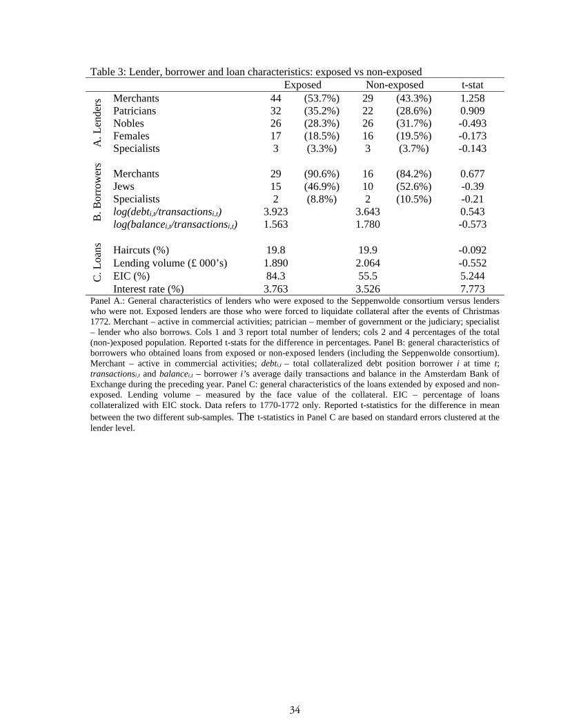
34

Table 3: Lender, borrower and loan characteristics: exposed vs non-exposed Exposed Non-exposed t-stat

A. L

ende

rs Merchants 44 (53.7%) 29 (43.3%) 1.258

Patricians 32 (35.2%) 22 (28.6%) 0.909 Nobles 26 (28.3%) 26 (31.7%) -0.493 Females 17 (18.5%) 16 (19.5%) -0.173 Specialists 3 (3.3%) 3 (3.7%) -0.143

B. B

orro

wer

s Merchants 29 (90.6%) 16 (84.2%) 0.677 Jews 15 (46.9%) 10 (52.6%) -0.39 Specialists 2 (8.8%) 2 (10.5%) -0.21 log(debti,t/transactionsi,t) 3.923 3.643 0.543 log(balancei,t/transactionsi,t) 1.563 1.780 -0.573

C. L

oans

Haircuts (%) 19.8 19.9 -0.092 Lending volume (£ 000’s) 1.890 2.064 -0.552 EIC (%) 84.3 55.5 5.244 Interest rate (%) 3.763 3.526 7.773

Panel A.: General characteristics of lenders who were exposed to the Seppenwolde consortium versus lenders who were not. Exposed lenders are those who were forced to liquidate collateral after the events of Christmas 1772. Merchant – active in commercial activities; patrician – member of government or the judiciary; specialist – lender who also borrows. Cols 1 and 3 report total number of lenders; cols 2 and 4 percentages of the total (non-)exposed population. Reported t-stats for the difference in percentages. Panel B: general characteristics of borrowers who obtained loans from exposed or non-exposed lenders (including the Seppenwolde consortium). Merchant – active in commercial activities; debti,t – total collateralized debt position borrower i at time t; transactionsi,t and balancei,t – borrower i’s average daily transactions and balance in the Amsterdam Bank of Exchange during the preceding year. Panel C: general characteristics of the loans extended by exposed and non-exposed. Lending volume – measured by the face value of the collateral. EIC – percentage of loans collateralized with EIC stock. Data refers to 1770-1772 only. Reported t-statistics for the difference in mean between the two different sub-samples. The t-statistics in Panel C are based on standard errors clustered at the lender level.

35

Table 4: Number of loans, lenders and borrowers, and collateral before/after Christmas 1772

Panel (A): Number of loan contracts by period From exposed Loans consortium Yes No yes no Before Xmas 1772 217 145 232 130 After Xmas 1772 41 15 . 56

Panel (B): Number of lenders and borrowers by period # of lenders; exposed # of borrowers; from exposed Yes No Yes No Before Xmas 1772 92 82 34 38 After Xmas 1772 18 10 21 11

# new lenders/borrowers after Xmas 1772

. 1 12 4

% loans accounted for by new lenders/borrowers

. 11% 44% 40%

Panel (C): Types of collateral used by period EIC BoE Other Lenders exposed Lenders exposed Lenders exposed yes no Yes no yes no Before Xmas 1772 84% 55% 14% 38% 2% 7% After Xmas 1772 83% 88% 0% 6% 17% 6% Sample characteristics before and after Christmas 1772. Panel (A) presents the number of new loans extended by type of lender and by whether loans were taken up by the Seppenwolde consortium. Exposed lenders are those who liquidated collateral after the default. Some loans taken up by the consortium were repaid before Christmas 1772. This explains why the total number of consortium loans is larger than the number of loans extended by exposed lenders. Panel (B) lists the number of lenders and borrowers, by type of lender. Borrowers are differentiated by whether they borrowed from exposed lenders. The panel also lists the number of new lenders and borrowers that entered the market after Christmas 1772. New borrowers are differentiated by whether they borrow from exposed or non-exposed lenders. We also calculate the percentage of total lending extended by new lenders / taken up by new borrowers, e.g. 44% of all loans extended by exposed lenders after 1772 went to new borrowers. Total lending is measured in face value of the collateral. Panel (C) presents the type of collateral that was used in the loan transactions, again differentiated by whether lenders were exposed yes or no. EIC is East India Company, BoE is Bank of England, Other includes South Sea Company (SSC) and a number of government securities. Table 5: Simple difference-in-difference estimate haircuts – EIC stock only Before Christmas 1772 After Christmas 1772 Not exposed 0.211 0.193 -0.018 Exposed 0.207 0.261 0.054***

-0.004 0.069*** 0.072*** Average haircuts on EIC stock, by exposed and non-exposed lenders, before and after Christmas 1772. Haircuts calculated as the fraction of the collateral value not financed with a loan. Exposed lenders -- those who forced to liquidate collateral after Christmas 1772. Each observation is a new contracts. Averages are weighed by the face value of collateral. The diff-in-diff estimate is in bold in the lower right corner. *** indicates significance at the 1% level.

36

Table 6: Benchmark estimates Panel A: Dependent Variable: Haircuts

(1)

OLS (2)

OLS (3) FE

(4) FE

(5) FE

Exposed -0.005 -0.003 -0.000 (0.005) (0.005) (0.006) Exposed * Post 1772 0.076 0.066 0.061 0.040 0.063 (0.022)*** (0.023)*** (0.036)* (0.024)* (0.036)* non-EIC -0.059 -0.056 -0.049 -0.052 -0.047 (0.006)*** (0.006)*** (0.011)*** (0.008)*** (0.014)*** Constant 0.219 0.245 0.235 0.211 0.174 (0.006)*** (0.017)*** (0.026)*** (0.012)*** (0.036)*** Adj. R2 0.334 0.440 0.632 0.659 0.802

Panel B: Dependent Variable: Interest rates

Exposed 0.072 0.048 0.074 (0.036)** (0.034) (0.041)* Exposed * Post 1772 -0.049 -0.034 -0.077 0.035 0.073 (0.099) (0.099) (0.130) (0.113) (0.219) non-EIC -0.078 -0.093 -0.084 -0.104 -0.078 (0.036)** (0.034)*** (0.050)* (0.049)** (0.053) Constant 3.527 3.637 3.739 3.559 3.879 (0.036)*** (0.096)*** (0.102)*** (0.071)*** (0.177)*** Adj. R2 0.511 0.564 0.744 0.699 0.836 Year dummies Y Y Y Y Y Lender type dummies N Y Y Borrower type dummies N Y Y

Lender FE N N Y N Y Borrower FE N N N Y Y N 418 387 418 387 418 N (if balanced) 166 77 33 # lenders 177 152 177 152 177 # borrowers 72 70 72 70 72 Regression estimates for all English securities. Observations refer to new contracts and are weighted by the face value of the collateral. Haircuts are calculated as the fraction of the collateral value that is not financed with a loan. Interest rates are annual. Exposed lenders are those who were forced to liquidate collateral after the events of Christmas 1772. Lender and borrower type dummies are as in Table 3. The interaction between the Exposed and the Post 1772 dummies captures the diff-in-diff effect. Lender and borrower fixed effects refer to fixed effects on the family/firm level. Robust standard errors (clustered at the lender level) are reported in parentheses. * p < 0.10, ** p < 0.05, *** p < 0.01

37

Table 7: Borrower attrition and riskiness Panel A: Attrition of borrowers after Christmas 1772 (logit, 1 = exit)

(1) (2) Incl. consortium Excl. consortium log(debti,t/transactionsi,t) 0.054 0.051 (0.049) (0.052) log(balancei,t/transactionsi,t) -0.143* -0.136 (0.083) (0.095) N 42 40 pseudo-R2 0.069 0.049

Panel B: Riskiness borrowers before/after Christmas 1772; exposed vs non-exposed (1) (2) (3) (4) (5) (6) log(debti,t/transactionsi,t) log(balancei,t /transactionsi,t) Exposed 0.493** 0.595*** -0.136 -0.276** (0.222) (0.220) (0.138) (0.110) Post 1772 0.322 0.928** 1.395*** 1.169** (0.383) (0.449) (0.183) (0.511) Exposed * Post 1772 -0.976 0.374 (0.678) (0.531) Constant 3.95*** 4.19*** 3.86*** 0.88*** 0.61*** 0.76*** (0.165) (0.112) (0.168) (0.105) (0.053) (0.083) N 337 337 337 337 337 337 Adj. R2 0.022 0.005 0.033 0.005 0.245 0.262 Panel A: logit estimates investigating whether a borrower drops out of the sample after Christmas 1772. , : total margin loan position borrower i at time t. balancei,t (transactionsi,t): average daily balance (transaction volume) of borrower i in the Amsterdam Bank of Exchange during the 52 weeks prior to time i. The table reports marginal effects, e.g. an increase in balance over transactions by one log point makes it 14% less likely that a borrower drops out of the sample. Panel B: OLS estimations at the loan level, investigating whether exposed and non-exposed lenders lent to different types of borrowers after Christmas 1772. Robust standard errors (clustered at the lender level) are reported in parentheses. * p < 0.10, ** p < 0.05, *** p < 0.01

38

Table 8: Lenders’ risk preferences (dependent variable: haircuts) Panel A: OLS Estimates: Sample Splits and Interactions

(1) (2) (3) (4) (5) (6) EIC share Interest (50)p (50)p (50)p (50)p

Exposed -0.003 -0.005 -0.005 -0.009 -0.009 -0.005 (0.006) (0.008) (0.006) (0.006) (0.012) (0.005) Exposed * Post 1772

0.048 (0.055)

0.067 (0.033)**

0.056 (0.033)*

0.037 (0.032)

0.093 (0.035)***

0.086 (0.027)***

Chi2 stat. 0.02 1.52 (p-value) (0.886) (0.217)

Non-EIC -0.052 -0.014 -0.055 -0.060 -0.053 -0.057 (0.009)*** (0.006)** (0.010)*** (0.008)*** (0.012)*** (0.006)***

_______ * Post 1772

0.040 (0.048)

-0.021 (0.025)

0.019 (0.021)

0.023 (0.030)

0.024 (0.025)

0.021 (0.018)

EIC share / Interest

0.005 (0.013)

0.009 (0.015)

_______ * Post 1772

0.041 (0.059)

-0.134 (0.061)**

N 188 199 384 186 201 381 Adj. R2 0.383 0.259 0.417 0.479 0.353 0.428

Panel B: Nearest Neighbor Matching Estimator ATT 0.068 0.055 0.078 0.072 0.062 0.063 (0.022)*** (0.022)** (0.020)*** (0.026)*** (0.014)*** (0.012)***

Additional matching

x EIC share

x Interest x x

variable Exact matching x x Decile x Decile Deciles variable(s) EIC Interest both share N 418 415 415 412 412 412 Panel A: Regression estimates for all English securities, weighted by the face value of the collateral. All specifications include year fixed effects and lender and borrower type dummies. The interaction between non-EIC and the Post 1772 dummy captures any changes in haircuts on collateral other than the EIC. EIC share is the proportion of a lender’s loan portfolio before 1773 that is collateralized with EIC stock. Interest is the average interest rate charged by a lender before 1773. Sample splits above and below the median investigate what part of the distribution the effect is coming from. We report a Chi2 test on whether the interaction effect is statistically different. The interaction term with the Post 1772 dummy captures whether lenders who seem to specialize in risky lending (more EIC as collateral, higher interest rates) adjust haircuts differently after Christmas 1772. Robust standard errors (clustered at the lender level) are reported in parentheses. Panel B: Nearest Neighbor Matching estimates using the face value of the collateral as weights, presenting the Average Effect for the Treated. Matching variables always included: Exposed, Post 1772, non-EIC, and year dummies. Robust standard errors presented in parentheses. * p < 0.10, ** p < 0.05, *** p < 0.01.

39

Table 9: Haircuts and time varying borrower riskiness (dependent variable: haircuts) (1) (2) (3) (4) (5) Exposed 0.001 0.002 -0.000 (0.006) (0.006) (0.006)

Exposed * Post 1772 0.052** 0.045** 0.101*** 0.077*** 0.054** (0.021) (0.019) (0.027) (0.023) (0.024)

non-EIC -0.050*** -0.051*** -0.045*** -0.047*** -0.053*** (0.008) (0.008) (0.014) (0.015) (0.008)

log(debti,t/transactionsi,t) 0.010** 0.010** 0.014*** 0.015*** (0.004) (0.004) (0.005) (0.005) __ * Post 1772 -0.017** -0.023** (0.009) (0.012)

log(balancei,t/transactionsi,t) -0.023*** -0.021* -0.027*** -0.026* (0.007) (0.011) (0.009) (0.015) __ * Post 1772 -0.017** -0.018 (0.008) (0.013) Year dummies Y Y Y Y Y Lender type dummies Y Y Y Borrower FE Y Y Y Y N Lender FE N N Y Y N Borrower-time FE N N N N Y N 317 317 341 341 381 Adj. R2 0.586 0.591 0.634 0.642 0.588 Regression estimates for all English securities. Observations refer to new contracts and are weighted by the face value of the collateral. Exposed lenders are forced to liquidate collateral after Christmas 1772. The interaction Exposed * Post 1772 captures the diff-in-diff effect. , : total margin loan position borrower i at time t. balancei,t (transactionsi,t): average daily balance (transaction volume) of borrower i in the Amsterdam Bank of Exchange during the 52 weeks prior to time i. Lender type dummies are as in Table 3. Borrower and lender FE refer to fixed effects on the family level. Robust standard errors (clustered at the lender level) in parentheses. * p < 0.10, ** p < 0.05, *** p < 0.01

40

Table 10: Probability of lender matching with a repeat borrower (1) (2) (3) (4) (5) (6) OLS OLS Logit Logit Probit Probit Post 1772 -0.211 -0.196 -0.211 -0.209 -0.211 -0.207 (0.050)*** (0.108)* (0.050)*** (0.110)* (0.050)*** (0.104)**

Exposed 0.026 0.020 0.021 (0.109) (0.086) (0.091)

Exposed * -0.018 -0.002 -0.006 Post 1772 (0.122) (0.196) (0.173) N 224 224 224 224 224 224 R2 0.050 0.050 Dependent variable: is a lender matched to a repeat borrower (one (s)he has lent to before) no=0; yes=1. Unit of observation: new loan contracts. To minimize measurement error of the repeat borrower variable, transactions after Jan 1, 1772 only. Post 1772 is a dummy for contracts signed after Christmas 1772. Exposed is a dummy for lenders who were exposed to the Seppenwolde bankruptcy. We report marginal effects. Estimates should be interpreted as the change in the probability of being matched with a repeat borrower in response to a change in the dummy variables from 0 to 1. Robust standard errors (clustered at the lender level) in parentheses. * p < 0.10, ** p < 0.05, *** p < 0.01 Table 11: Haircuts and lender characteristics (dependent variable: haircuts) (1) (2) (3) (4) (5) (6) Lender group: Merchant Patrician Noble Female Specialist All Exposed -0.002 -0.003 -0.003 -0.003 -0.003 -0.003 (0.005) (0.005) (0.004) (0.005) (0.005) (0.005)

Exposed * Post 1772 0.062 0.068 0.062 0.064 0.065 0.061 (0.021)*** (0.023)*** (0.023)*** (0.022)*** (0.023)*** (0.021)***

non-EIC -0.055 -0.056 -0.056 -0.056 -0.056 -0.056 (0.006)*** (0.006)*** (0.006)*** (0.006)*** (0.006)*** (0.006)***

Lender group 0.033 -0.015 -0.040 -0.026 0.005 * Post 1772 (0.019)* (0.017) (0.019)** (0.029) (0.047)

Constant 0.241 0.243 0.239 0.244 0.245 0.239 (0.018)*** (0.017)*** (0.017)*** (0.017)*** (0.017)*** (0.018)***

Year dummies Y Y Y Y Y Y Lender & borrower observables

Y Y Y Y Y Y

N 387 387 387 387 387 387 R2 0.448 0.442 0.452 0.443 0.440 0.453 # lenders 152 152 152 152 152 152 Pooled OLS estimates for all English securities. Observations refer to new contracts and are weighted by the face value of the collateral. Haircuts are calculated as the fraction of the collateral value that is not financed with a loan. Exposed lenders are those who were forced to liquidate collateral after the events of Christmas 1772. The interaction between the Exposed and the Post 1772 dummies captures the diff-in-diff effect. Lender and borrower observables are as in Table 3. Merchant – active in commerce; patrician – member of (local) government or judiciary; specialist – lenders also active as borrower. Col (6) contains dummies for all borrower groups. Robust standard errors (clustered at the lender level) are reported in parentheses. * p < 0.10, ** p < 0.05, *** p < 0.01