Embed Size (px)
Citation preview
LethbridgeAdvancedAbstractAlgebra
Dave Witte MorrisUniversity of Lethbridge, Canada
September 8, 2021
To the extent possible under law, Dave Witte Morris has waivedall copyright and related or neighboring rights to this work.
You can copy, modify, and distribute this work, even for commercial purposes, all without askingpermission. For more information, visithttp://creativecommons.org/publicdomain/zero/1.0/

Contents
Part I. Group Theory 1
Chapter 1. Summary of undergraduate group theory 31.1. Definitions and examples 31.2. Burnside’s Counting Lemma (optional) 91.3. Subgroups, conjugates, cosets, and quotient groups 121.4. Homomorphisms and isomorphisms 15
Chapter 2. Group Actions 192.1. Definition and basic facts 192.2. Orbits and stabilizers 202.3. Sylow Theorems 23
Chapter 3. Series of subgroups 273.1. Solvable groups and subnormal series 283.2. Nilpotent groups and central series (advanced) 303.3. Lower central series and upper central series (optional) 343.4. Supersolvable groups (optional) 353.5. Simple groups and composition series 36
Chapter 4. Constructions of groups 394.1. Informal look at groups defined by generators and relations 394.2. Free groups and the proof of Von Dyck’s Theorem (advanced) 424.3. Semidirect products (optional) 44
Part II. Rings and Modules 47
Chapter 5. Summary of undergraduate ring theory 495.1. Elementary facts and definitions 495.2. Homomorphisms and isomorphisms 515.3. PIDs, UFDs, and Euclidean domains 525.4. Rings in number theory (optional) 555.5. Fields and polynomials 57
Chapter 6. Modules over a ring 616.1. Definition and basic facts 616.2. Submodules, quotients, homomorphisms, and annihilators 626.3. Isomorphism Theorems and the Correspondence Theorem 656.4. Free modules and direct products 66
Chapter 7. Modules over a PID 697.1. Torsion modules over a PID 697.2. Completion of the proof of the Structure Theorem 737.3. Fundamental Theorem of Finitely Generated Abelian Groups 757.4. Zorn’s Lemma (advanced) 77
iii
iv CONTENTS
Part III. Linear Algebra 81
Chapter 8. Review 838.1. Basis, dimension, coordinates, etc. 838.2. Determinants, eigenvalues, and eigenvectors 858.3. Diagonalizability 88
Chapter 9. Bilinear forms and Hermitian forms 919.1. Real symmetric matrices are diagonalizable (optional) 919.2. Bilinear forms 939.3. Dual space V∗ 949.4. Hermitian forms and diagonalizability 969.5. Tensor products of vector spaces (advanced) 99
Chapter 10. Jordan Canonical Form 10510.1. What is Jordan Canonical Form, and what is it good for? 10510.2. Proof that matrices have a Jordan Canonical Form 109
Index 113
Part I
Group Theory

Chapter 1
Summary ofundergraduate group theory
Although this course assumes familiarity with the topics in a typical undergraduate course onabstract algebra, including subgroups, normal subgroups, homomorphisms, quotient groups, etc.,we will start with a quick review.
(1.0.1) Notation.
• G is always a group, and X is a set.
• The cardinality of X is denoted |X| (or, sometimes, #X). (Recall that the cardinality of aset is the number of elements in the set.)
• Z = {. . . ,−3,−2,−1,0,1,2,3, . . .}.• N = {0,1,2, . . .} (unlike some other authors, we include 0 in this set).
• Z+ = N+ = {1,2,3, . . .}.• For k,n ∈ Z, we write k | n to denote that k is a divisor of n (or, equivalently, that n is a
multiple of k).• For a,b,n ∈ Z, we write a ≡ b (mod n) to denote that n | (a− b), and we may say that a
is congruent to b, modulo n.
§1.1. Definitions and examples
(1.1.1) Definition. A group is a set G together with a binary operation ∗ that is associative andhas an identity element and inverses. (We usually write gh, or sometimes g · h, for g ∗ h.)
• (associative) ∀g1, g2, g3 ∈ G, g1(g2g3) = (g1g2)g3.
• (identity element) ∃e ∈ G,∀g ∈ G, eg = ge = g.
It is easy to show that the identity element of G is unique (see Example 1.1.2(1)). Itis usually denoted by 1 or, sometimes, e. (However, it is denoted by 0 if G is writtenadditively, which means that the group operation is +.) To avoid confusion, we willsometimes use 1G for the identity element of G (and 1H for the identity element ofsome other group H).
• (inverses) ∀g ∈ G,∃h ∈ G, gh = hg = 1.
It is easy to show that the inverse of g is unique (see Example 1.1.2(2)). It is denotedg−1 (unless G is written additively, in which case the inverse is −g) .
3

4 1. SUMMARY OF UNDERGRADUATE GROUP THEORY
(1.1.2) Example. We verify two facts stated in Definition 1.1.1, and also establish two facts ofhigh-school algebra.
1) If e1 and e2 are identity elements of G, then e1 = e2. To see this, note that:
e1 = e1e2 (e2 is an identity element, so ge2 = g for all g ∈ G)
= e2 (e1 is an identity element, so e1g = g for all g ∈ G).2) Assume that G has an identity element 1, and let g ∈ G. If h1 and h2 are inverses of g, thenh1 = h2. To see this, note that:
h1 = h1 ∗ 1 (1 is the identity element, so h∗ 1 = h for all h ∈ G)
= h1 ∗ (g ∗ h2) (h2 is an inverse of g)
= (h1 ∗ g)∗ h2 (∗ is associative)
= 1∗ h2 (h1 is an inverse of g)
= h2 (1 is the identity element, so 1∗ h = h for all h ∈ G).3) The inverse of a product is the product of the inverses in the reverse order:
(gh)−1 = h−1g−1.To see this, note that
(gh)(h−1g−1) = g(hh−1)g−1 = g · 1 · g−1 = gg−1 = 1.A similar calculation shows that (h−1g−1)(gh) = 1. Thus, we have shown that if youmultiply gh by h−1g−1 on either side, then the result is the identity element. This is exactlywhat it means to say that h−1g−1 is the inverse of gh.
4) G has both right and left cancellation: if ag = ah or ga = ha, then g = h. To see this,note that if ag = ah, then a−1(ag) = a−1(ah). Furthermore (using the associative law) theleft-hand side is 1 · g = g and the right-hand side is 1 · h = h, so we conclude that g = h,as desired. Similarly, if ga = ha, then
g = g · 1 = (ga)a−1 = (ha)a−1 = h · 1 = h.(1.1.3) Definitions. Let g, h, and a be elements of a group G.
1) The cardinality of the set G is called the order of G. It is denoted |G|.2) For k ∈ Z+, we define gk to be the product of k copes of g: we have gk = gg · · ·g, where
there are k factors on the right-hand side. And we let g−k = (gk)−1 (or (g−1)k, which is thesame thing, by Example 1.1.2(3)). Finally, we let g0 = 1. With these definitions, the usuallaws of exponents hold (for k,ℓ ∈ Z):
g0 = 1, g1 = g, gkgℓ = gk+ℓ, (gk)ℓ = gkℓ, (gk)−1 = (g−1)k.(If the group operation is +, then we write kg for g + g + · · · + g, instead of gk.)
3) The order of g is the smallest k ∈ Z+, such that gk = 1. It is denoted |g|. (If no such kexists, then |g| = ∞.)
4) g and h commute if gh = hg. (We may also say that g centralizes h.) We say that G isabelian (or commutative) if all the elements of G commute with each other.
(1.1.4) Exercise. Let g ∈ G, such that g has finite order.
1) For k,ℓ ∈ Z, show:(a) gk = 1 if and only if k is a multiple of |g|.(b) More generally, gk = gℓa k ≡ ℓ (mod |g|).
2) Show |g−1| = |g|.In this course, we will mostly be interested in finite groups. (These are groups that have only
finitely many elements, or in other words, the groups whose order is finite.) It is important to befamiliar with some examples.
1.1. DEFINITIONS AND EXAMPLES 5
(1.1.5) Example (Integers modulonunder addition). Recall that Zn is the set of integers modulo n.This means that elements of Zn are integers, except that we consider two elements of Zn to beequal if they are congruent modulo n. More precisely, the elements of Zn are equivalence classesof integers, where two integers are equivalent if they have the same remainder when you dividethem by n. We can use k to represent the equivalence class of k in Zn. For example,
Z2 = {0,1},Z3 = {0,1,2},Z4 = {0,1,2,3},Z5 = {0,1,2,3,4},Z6 = {0,1,2,3,4,5}, etc.
Each of these is a group under addition modulo n, which is defined by k+ ℓ = k+ ℓ:1) (associative) In elementary school, we all learned the associative law (for the addition of
ordinary integers). This implies that addition modulo n is also associative:(k+ ℓ)+m = k+ ℓ+m (definition of addition in Zn)
= (k+ ℓ)+m (definition of addition in Zn)
= k+ (ℓ+m) (associate law for addition in Z)
= k+ ℓ+m (definition of addition in Zn)
= k+ ℓ+m (definition of addition in Zn).
2) (identity element) The additive identity element of Z is 0, so the identity element of Zn is 0:
k+ 0 = k+ 0 = k and 0+ k = 0+ k = k.3) (inverses) The (additive) inverse of k in Z is −k so the inverse of k in Zn is −k:
k+−k = k+ (−k) = 0 and −k+ k = (−k)+ k = 0.Note that, for the element 1 ∈ Zn, we have |1| = n.
(1.1.6) Exercise. The direct product of two groups G and H is the Cartesian product G ×H withcomponentwise multiplication. That is, (g1, h1)∗ (g2, h2) = (g1g2, h1h2).
1) Show that G ×H is a group.[Hint: By definition, this means you need to show that the operation is associative, and has an identity elementand inverses.]
2) For (g,h) ∈ G ×H, show that |(g,h)| is the least common multiple of |g| and |h|.(1.1.7) Example. Z3 × Z5 × Z7 is a group of order 3 · 5 · 7 = 105. In this group, we have
(2,4,5)+ (2,1,4) = (2+ 2,4+ 1,5+ 4) = (2+ 2,4+ 1,5+ 4) = (4,5,9) = (1,0,2).(1.1.8) Exercise (semidirect product of cyclic groups). Supposem,n ∈ Z+, and let k ∈ Z, such thatkn ≡ 1 (modm). Define a binary operation on the set Zm × Zn by
(x1, y1)∗ (x2, y2) = (x1 + ky1 x2, y1 +y2).Show that this operation is associative, and has an identity element and inverses. Hence, it definesa group (of order mn).
This group is called the semidirect product of Zm and Zn (with multiplier k), and is denotedZm ⋊k Zn. It is a generalization of the the direct product of Zm and Zn, which is the special casewhere k = 1. (See Section 4.3 for a further generalization, which replaces Zm and Zn with othergroups.)
(1.1.9) Example. In Z7 ×4 Z3, we have
(3,2)∗ (5,1) = (3+ 42 · 5, 2+ 1) = (3+ 42 · 5, 2+ 1) = (83, 3) = (6, 0).
Groups often arise as symmetries of an object.
(1.1.10) Definition (informal). A symmetry of an object is a way of repositioning the object insuch a way that it occupies exactly the same space as it did originally. It is sometimes called an“undetectable motion:” if you perform a symmetry to an object while someone is not looking, theywill not realize that anything has changed, because everything looks exactly as it did before.
6 1. SUMMARY OF UNDERGRADUATE GROUP THEORY
(1.1.11) Example (Rotations of a square). Imagine a square lying on a tabletop. Rotating the squareby 90◦ is a symmetry of the square. For short, let us use rθ to denote a rotation by θ degrees(clockwise). So r90 is a symmetry of the square. Other symmetries are r180 and r270. (By theway, another name for r270 is r−90. Or we could rotate by 0◦ (doing nothing certainly leaves thesquare occupying the same space as it did before), so r0 = r360 is also a symmetry of the square.There are no other rotational symmetries, so the rotational symmetries of the square form the set{r0, r90, r180, r270}.
It is important to note that this set is a group under composition, or, in the language of non-mathematicians, the “after” operation: recall that r ◦ s is the procedure that is obtained by doingr after s: first apply s to the object, then apply s. For example, r90 ◦ r180 = r270, because rotatingthe square by 90 degrees after rotating it by 180 degrees has exactly the same effect as applying asingle rotation of 180 degrees to the square. Note that this is a group of order 4. We have |r0| = 1,|r90| = |r270| = 4, and |r180| = 2.
In general, the symmetries of an object always form a group.
(1.1.12) Remark. It is not difficult to verify the above statement that symmetries form a group:
• To see that composition is a binary operation on the set of symmetries, we need to knowthat the set of symmetries is closed under composition: if r and s are symmetries ofan object X, then r ◦ s is also a symmetry of X. Fortunately, this is clearly true: if wereposition X in some way that is undetectable, and then reposition it again in a way that isundetectable, then the final position is also indistinguishable from the original position.
• Composition is associative: r ◦(s◦t) = (r ◦s)◦t. This is because it does not matter whetherwe :◦ first do t, then do s, and then take a break before doing r , or◦ first do t, then take a break before doing s and then r .
In either case, we are doing t, and then s, and then r .
• The identity element of the group is the “do nothing” operation.
• The inverse of a particular symmetry is “put it back the way it was.”
The square can be replaced with any regular polygon:
(1.1.13) Example. The set of rotations of a regular n-gon P is a group Rot(P) of order n. Moreprecisely, if θ = 360/n, then
Rot(P) = {r0, rθ, r2θ, . . . , r(n−1)θ}.Furthermore, we have rkθ ◦ rℓθ = r(k+ℓ)θ, and r−1
kθ = r−kθ.(1.1.14) Exercise. Find the order of each of the six rotations of the regular hexagon.
But rotations are not the only symmetries of a regular n-gon:
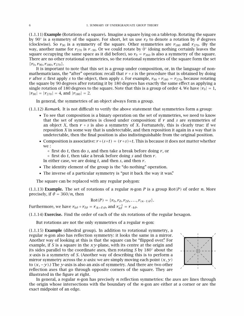
(1.1.15) Example (dihedral group). In addition to rotational symmetry, aregular n-gon also has reflection symmetry: it looks the same in a mirror.Another way of looking at this is that the square can be “flipped over.” Forexample, if S is a square in the xy-plane, with its centre at the origin andits sides parallel to the coordinate axes, then rotating S by 180◦ about thex-axis is a symmetry of S. (Another way of describing this is to perform amirror symmetry across the x-axis: we are simply moving each point (x,y)to (x,−y).) The y-axis is also an axis of symmetry. And there are two otherreflection axes that go through opposite corners of the square. They areillustrated in the figure at right.
In general, a regular n-gon has precisely n reflection symmetries: the axes are lines throughthe origin whose intersections with the boundary of the n-gon are either at a corner or are theexact midpoint of an edge.
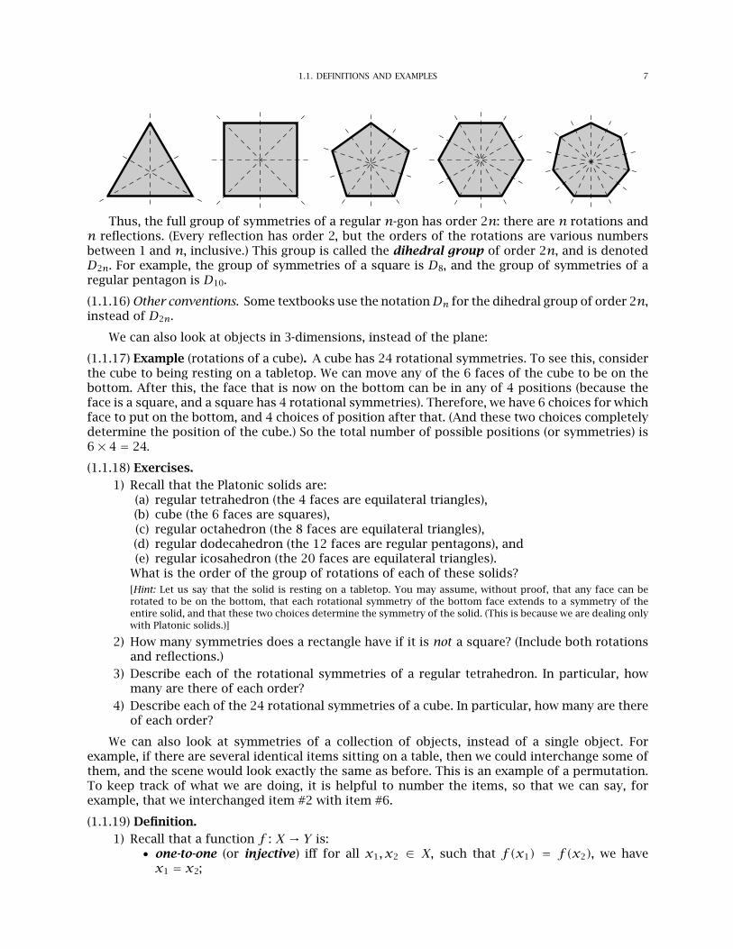
1.1. DEFINITIONS AND EXAMPLES 7
Thus, the full group of symmetries of a regular n-gon has order 2n: there are n rotations andn reflections. (Every reflection has order 2, but the orders of the rotations are various numbersbetween 1 and n, inclusive.) This group is called the dihedral group of order 2n, and is denotedD2n. For example, the group of symmetries of a square is D8, and the group of symmetries of aregular pentagon is D10.
(1.1.16) Other conventions. Some textbooks use the notationDn for the dihedral group of order 2n,instead of D2n.
We can also look at objects in 3-dimensions, instead of the plane:
(1.1.17) Example (rotations of a cube). A cube has 24 rotational symmetries. To see this, considerthe cube to being resting on a tabletop. We can move any of the 6 faces of the cube to be on thebottom. After this, the face that is now on the bottom can be in any of 4 positions (because theface is a square, and a square has 4 rotational symmetries). Therefore, we have 6 choices for whichface to put on the bottom, and 4 choices of position after that. (And these two choices completelydetermine the position of the cube.) So the total number of possible positions (or symmetries) is6× 4 = 24.
(1.1.18) Exercises.1) Recall that the Platonic solids are:
(a) regular tetrahedron (the 4 faces are equilateral triangles),(b) cube (the 6 faces are squares),(c) regular octahedron (the 8 faces are equilateral triangles),(d) regular dodecahedron (the 12 faces are regular pentagons), and(e) regular icosahedron (the 20 faces are equilateral triangles).
What is the order of the group of rotations of each of these solids?[Hint: Let us say that the solid is resting on a tabletop. You may assume, without proof, that any face can berotated to be on the bottom, that each rotational symmetry of the bottom face extends to a symmetry of theentire solid, and that these two choices determine the symmetry of the solid. (This is because we are dealing onlywith Platonic solids.)]
2) How many symmetries does a rectangle have if it is not a square? (Include both rotationsand reflections.)
3) Describe each of the rotational symmetries of a regular tetrahedron. In particular, howmany are there of each order?
4) Describe each of the 24 rotational symmetries of a cube. In particular, how many are thereof each order?
We can also look at symmetries of a collection of objects, instead of a single object. Forexample, if there are several identical items sitting on a table, then we could interchange some ofthem, and the scene would look exactly the same as before. This is an example of a permutation.To keep track of what we are doing, it is helpful to number the items, so that we can say, forexample, that we interchanged item #2 with item #6.
(1.1.19) Definition.1) Recall that a function f : X → Y is:
• one-to-one (or injective) iff for all x1, x2 ∈ X, such that f(x1) = f(x2), we havex1 = x2;
8 1. SUMMARY OF UNDERGRADUATE GROUP THEORY
• onto (or surjective) iff for all y ∈ Y , there exists x ∈ X, such that f(x) = y;• a bijection iff f is both one-to-one and onto.
2) A permutation of X is a bijection from X to itself.
3) The set of all permutations of X is called the symmetric group on X. It is a group undercomposition (see Exercise 1.1.24): (στ)(x) = σ(τ(x)) for all x ∈ X.
4) The symmetric group on {1,2, . . . , n} is called the symmetric group on n letters (or “ofdegree n”), and is denoted Sn. Its order is n!.
5) For x1, . . . , xk ∈ X, we use (x1 x2 . . . xk) to denote the unique permutation σ ∈ Sn, suchthat• σ(xi) = xi+1 for i ∈ {1, . . . , k} (reading the subscript modulo k), and• σ(x) = x for all x ∉ {x1, x2, . . . , xk}.
Such a permutation is called a cycle of length k, or a k-cycle.
6) Two cycles (x1 x2 . . . xk) and (y1y2 . . . yℓ) are disjoint if the sets {x1, x2, . . . , xk} and{y1, y2, . . . , yℓ} are disjoint (that is, they have no elements in common).
Dealing with permutations requires some basic facts from Math 2000. If you have difficultywith the definition, or the subsequent exercises, you may want to review a textbook for that course.One such textbook is available online at:
http://people.uleth.ca/~dave.morris/books/proofs+concepts.html
(1.1.20) Definition. Assumeφ : X → Y and σ : Y → Z. The composition of σ andφ is the functionσ ◦φ from X to Z that is defined by
(σ ◦φ)(x) = σ(φ(x)) for all x ∈ X.(1.1.21) Exercises (Basic properties of composition). Assume φ : X → Y and σ : Y → Z.
1) Prove that composition is associative: show that if, in addition toφ : X → Y and σ : Y → Z,we also have τ : Z → W , then (τ ◦ σ) ◦φ = τ ◦ (σ ◦φ). (This was explained informally inRemark 1.1.12, but you should be able to write an official proof of this fact.)
2) Show that the composition of one-to-one functions is one-to-one: ifφandσ are one-to-one,then σ ◦φ is one-to-one.
3) Show that the composition of onto functions is onto: if φ and σ are onto, then σ ◦φ isonto.
4) Show that the composition of bijections is a bijection: ifφ and σ are bijections, then σ ◦φis a bijection.[Hint: Use (2) and (3).]
Bijections arise in many situations, but one of their most important applications is in showingthat two sets have the same cardinality:
(1.1.22) Basic facts.
1) Definition. Two sets X and Y have the same cardinality if and only if there is a bijectionfrom X to Y .
2) Assume φ : X → Y , and let A be any subset of X.(a) Definition. f(A) = {f(a) | a ∈ A }. (This is called the image of A under f .)(b) If φ is one-to-one, then |f(A)| = |A|.
It is not difficult to see if φ : X → Y has an inverse φ−1 : Y → X, then φmust be a bijection.It is an important fact from Math 2000 that the converse is true. However, this is more difficult,so you do not need to try to prove it for yourself, although you should remember this importantfact:
(1.1.23) Basic fact. If φ : X → Y is a bijection, then φ has an inverse φ−1 : Y → X.
Some of the above facts will be helpful in solving the following problem:
1.2. BURNSIDE’S COUNTING LEMMA (optional) 9
(1.1.24) Exercise. Prove that the symmetric group SX is indeed a group (under composition).Also show that the identity element of this group is the identity map on X. (The identity map
on X is the function 1X : X → X defined by 1X(x) = x for x ∈ X.)
(1.1.25) Basic facts.1) If two cycles are disjoint, then they commute with each other.2) Every permutation of a finite set is a product of disjoint cycles. Furthermore, this
decomposition into disjoint cycles is unique, up to a permutation of the factors.
(1.1.26) Example. (1 3)(2 5 7) is an element of S7. (In fact, it is an element of Sn for any n ≥ 7.) Itsaction on the elements of {1,2,3,4,5,6,7} is:
1 , 3, 2 , 5, 3 , 1, 4 , 4, 5 , 7, 6 , 6, 7 , 2.This permutation has order 6. (In general, the order of a permutation is the least common multipleof the lengths of the cycles in its decomposition as a product of disjoint cycles.)
(1.1.27) Exercise. In each part of the problem, write each of the given permutations as a productof disjoint cycles. Also find the order of each of the permutations.
1) (1 2)(2 3)(3 4). 2) (1 2)(1 3)(1 4)(1 5). 3) (2 3 5)(2 3 4)(1 4 2 5 3).
4) Number the corners of a regular hexagon from 1 to 6, clockwise, so that we may think ofeach of its six rotational symmetries as elements of S6. You are to consider all six of thesepermutations.
5) Number the corners of a square from 1 to 4, clockwise, so that we may think of each ofthe elements of D8 as elements of S4. The permutations to consider are:(a) the reflection whose axis is through corners 1 and 3, and(b) the reflection whose axis is through the midpoints of sides 1−2 and 3−4.
§1.2. Burnside’s Counting Lemma (optional)
(1.2.1) Problem. We have five colours of paint available with which to paint the faces of a cube.(Every face needs to be painted, and only one colour is allowed to appear on each face, but severalfaces may be painted the same colour, and it is not necessary to use all 5 colours.) How manyessentially different ways are there to paint the cube?
High-school-level mathematics reveals there are exactly 56 = 15,625 ways to paint the facesof the cube, because we can use any one of 5 colours of paint on each of the 6 faces of the cube.However, this is not the answer we want. For example, suppose Alice paints the top face of hercube blue and all of the other faces red, while Bob paints the bottom of his cube blue and all theother faces red. Then Alice and Bob have painted their cubes in essentially the same way — ifAlice turns her cube upside-down, then it looks just like Bob’s.
If there were only two colours of paint, it would not be difficult to solve the problem by listingall of the possible colourings. But that is not very feasible for five colours (unless a computer isused). This section presents a method that easily solves this problem and many related types ofproblems, by applying the theory of group actions.
We will see the official definitions in Section 2.1, but, for now, it will suffice to have an informalunderstanding of two key ideas:
• Saying that a groupGacts on a setXmeans that each element g ofG acts like a permutationof the elements of a set X: the group element g carries each x ∈ X to some point that iscalled gx.
• Each x in X can be moved to certain other places in X. (But probably there are places thatG cannot move it to. For example, rotations of a square cannot move a corner point to apoint that is not on a corner.) The set of points that x can move to is called the orbit of x.
(1.2.2) Definition. Suppose G acts on X. For g ∈ G and x ∈ X, we say that x is a fixed point of gif gx = x. (This means that g leaves x alone, instead of moving it somewhere else.)
10 1. SUMMARY OF UNDERGRADUATE GROUP THEORY
(1.2.3) Proposition (Burnside’s Counting Lemma). Suppose G acts on a finite set X (and G is finite).Then the number of orbits of G on X is equal to the number of fixed points of the average elementof G.
(1.2.4) Remark. To be precise, the phrase “the number of fixed points of the average elementof G,” actually means “the average of the numbers of fixed points of elements of G.” That is, list thenumber of fixed points of each element of G, and then calculate the average (or arithmetic mean)of these numbers.
We will see some applications of this proposition right now, but the proof will be postponeduntil Section 2.2, when we have more tools from the theory of group actions.
(1.2.5) Examples.
1) Suppose every element of G leaves all of the points of X alone. (This could be called the“lazy” group action, because the elements ofG are too lazy to do anything, but it is officiallycalled the trivial action of G.) Then each element of X constitutes an orbit, so the numberof orbits is |X|. On the other hand, each element of G fixes every point in X, so the numberof fixed points of each element (including the average element) is also |X|. This agrees withthe conclusion of Burnside’s Counting Lemma.
2) Let G = Rot(cube) and let X be the set of faces of the cube. Only the identity element of Gfixes every face of the cube, while there are 9 rotations that fix two faces (six rotations oforder 4, and three rotations of order 2), and all other elements of G have no fixed pointsin the action on X. So the number of fixed points of the average element of G is
1× 6+ 9× 2+ 14× 024
= 1.
Also, any face of the cube can be moved to any other face by a rotation, so this actionhas only 1 orbit. Hence, we once again have agreement with the conclusion of Burnside’sCounting Lemma.
3) Let G be the group of symmetries of a rectangle (which is not a square), and let X be the setof sides of the rectangle. The rectangle has only four symmetries (see Exercise 1.1.18(2)):• The trivial symmetry (do nothing) fixes all 4 sides.• r180 does not fix any sides, so the number of sides that are fixed is 0.• Each of the two reflection symmetries fixes the 2 sides that are on its axis (and
interchanges the other two).So the number of fixed points of the average element of G is
1× 4+ 1× 0+ 2× 24
= 2.
Also the long sides of the rectangle can be moved to each other, and the short sides ofthe rectangle can be moved to each other, but a symmetry cannot move a long side so ashort side. So there are 2 orbits. Therefore, of course, we yet again have agreement withthe conclusion of Burnside’s Counting Lemma.
Solution to Problem 1.2.1. Two colourings of the cube are essentially different if there is norotation of the cube that takes one to the other, that is, if they are in different orbits in the actionof Rot(cube)on the collection of colourings of the cube. So the total number of essentially differentcolourings of the cube is equal to the number of orbits of Rot(cube) on the set of colourings. ByBurnside’s Counting Lemma, this is the same as the number of colourings fixed by an averageelement of Rot(cube).
Any permutation can be uniquely expressed as a product of disjoint cycles, and it is easy tosee that such a permutation will fix a colouring if and only if each cycle of the permutation ismonochromatic. (That is, all of the faces in each cycle must have the same colour, but faces indifferent cycles may have different colours.) Thus, if there are k colours available, then the numberof colourings fixed by the permutation g is kcyc(g), where cyc(g) is the number of cycles in thedisjoint cycle decomposition of g. Therefore, applying Burnside’s Counting Lemma tells us:
1.2. BURNSIDE’S COUNTING LEMMA (optional) 11
The number of essentially different ways to paint the faces of a cube with k colours is1
|Rot(cube)|∑
g∈Rot(cube)
kcyc(g).
To calculate the sum, we count the cycles in each element of Rot(cube):1) The identity element fixes all 6 faces, so it has 6 cycles of length one.2) 3 elements are rotations of 180◦ about an axis through opposite faces of the cube. These
have 2 cycles of length one, and 2 cycles of length two, for a total of 4 cycles.3) 6 elements are 90◦ rotations. They have 2 cycles of length one, and 1 cycle of length four,
for a total of 3 cycles.4) 6 elements are 180◦ rotations about an axis through opposite edges. They have 3 cycles,
all of length two.5) 8 elements are rotations about an axis through opposite corners. They have 2 cycles of
length three.So the number of essentially different colourings is
k6 + 3k4 + 6k3 + 6k3 + 8k2
24. (1.2.6)
We plug in k = 5 to get 800 as the answer to the original problem. □
(1.2.7) Remark. Letting k = 1 in (1.2.6) yields the value 1. This agrees with the observation thatthere is only one way to colour the faces of a cube if only one colour of paint is available. (Theentire cube must be covered with that one colour.)
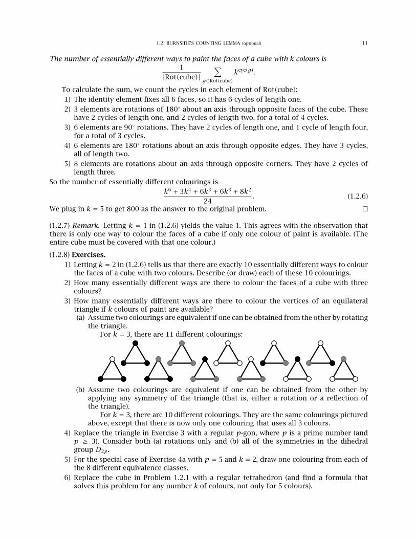
(1.2.8) Exercises.1) Letting k = 2 in (1.2.6) tells us that there are exactly 10 essentially different ways to colour
the faces of a cube with two colours. Describe (or draw) each of these 10 colourings.2) How many essentially different ways are there to colour the faces of a cube with three
colours?3) How many essentially different ways are there to colour the vertices of an equilateral
triangle if k colours of paint are available?(a) Assume two colourings are equivalent if one can be obtained from the other by rotating
the triangle.For k = 3, there are 11 different colourings:
(b) Assume two colourings are equivalent if one can be obtained from the other byapplying any symmetry of the triangle (that is, either a rotation or a reflection ofthe triangle).
For k = 3, there are 10 different colourings. They are the same colourings picturedabove, except that there is now only one colouring that uses all 3 colours.
4) Replace the triangle in Exercise 3 with a regular p-gon, where p is a prime number (andp ≥ 3). Consider both (a) rotations only and (b) all of the symmetries in the dihedralgroup D2p.
5) For the special case of Exercise 4a with p = 5 and k = 2, draw one colouring from each ofthe 8 different equivalence classes.
6) Replace the cube in Problem 1.2.1 with a regular tetrahedron (and find a formula thatsolves this problem for any number k of colours, not only for 5 colours).
12 1. SUMMARY OF UNDERGRADUATE GROUP THEORY
§1.3. Subgroups, conjugates, cosets, and quotient groups
(1.3.1) Definitions (subgroups).
1) A subset H of G is a subgroup of G if it is closed under the group operations: for allh1, h2, h ∈ H, we have h1h2 ∈ H and h−1 ∈ H (and 1 ∈ H). Equivalently, this means thatH is itself a group under the operation obtained by restricting the operation of G.
(For example, if P is a regular n-gon, then Rot(P) is a subgroup of D2n.)
2) The obvious subgroups of G are {1} and G. (There may or may not be other subgroupsof G.)• {1} is the trivial subgroup of G. (All other subgroups are nontrivial .)• A subgroup H of G is said to be proper if H ≠ G.
3) For g ∈ G, we let ⟨g⟩ = {gk | k ∈ Z }. This is an abelian subgroup ofG (see Exercises 1.3.4(1)and 1.3.5(1)), and is called the cyclic subgroup generated by g.
4) We say G is cyclic if G = ⟨g⟩ for some g ∈ G. For example, Zn is cyclic (for every n ∈ Z+),because Zn = ⟨1⟩.
(1.3.2) Example. If H1 and H2 are subgroups of G, then H1 ∩H2 is a subgroup of G.
Proof. We wish to show that H1∩H2 is closed under multiplication and inverses, and contains theidentity element.
(closed under multiplication) Given g,h ∈ H1 ∩ H2 we have g,h ∈ H1 and g,h ∈ H2. Sinceeach Hi is a subgroup, and is therefore closed under multiplication, this implies that gh ∈ H1 andgh ∈ H2. So gh ∈ H1 ∩H2, as desired.
(closed under multiplication) Given h ∈ H1 ∩H2 we have h ∈ H1 and h ∈ H2. Since each Hi isa subgroup, and is therefore closed under inverses, this implies that h−1 ∈ H1 and h−1 ∈ H2. Soh−1 ∈ H1 ∩H2, as desired.
(identity element) Since eachHi is a subgroup, it must contain the identity element. This meansthat 1 ∈ H1 and 1 ∈ H2. So 1 ∈ H1 ∩H2, as desired. □
(1.3.3) Remark. By induction, Example 1.3.2 implies that the intersection of any finite collectionof subgroups of G is a subgroup of G, because H1∩H2∩· · ·∩Hn = (H1∩H2∩· · ·∩Hn−1)∩Hnis the intersection of two subgroups. But it is not difficult to show directly that the intersectionof any collection of subgroups is also a subgroup, even if the collection is infinite.
(1.3.4) Exercise. Here are some important subgroups of G:
1) Let g ∈ G. Show that ⟨g⟩ is a subgroup of G.
2) For any subset S of G, the centralizer of S in G is
CG(S) = {g ∈ G | g commutes with every element of S }.Show that CG(S) is a subgroup of G.
3) For any subgroup H of G, the normalizer of H in G is
NG(H) = {g ∈ G | gH = Hg },where gH = {gh | h ∈ H } and Hg = {hg | h ∈ H }. Show that NG(H) is a subgroup of G.
4) The centre of G is
Z(G) = CG(G) = {z ∈ G | zg = gz for all g ∈ G}.Show that this is an abelian, normal subgroup of G.
(1.3.5) Exercises.
1) Show that every cyclic group is abelian.
2) For g ∈ g, show that |g| = |⟨g⟩|. More precisely, show that ⟨g⟩ = {gk | 0 ≤ k < |g| }, andthat all of these elements are distinct.[Hint: Item 1(1b).]
1.3. SUBGROUPS, CONJUGATES, COSETS, AND QUOTIENT GROUPS 13
(1.3.6) Exercise. Suppose H and K are subgroups of G, and let HK = {hk | h ∈ H, k ∈ K }. Showthat HK is a subgroup of G if and only if HK = KH.
(1.3.7) Definitions.
1) For any subset S of G, we use ⟨S⟩ to denote the (unique) smallest subgroup of G thatcontains S. This is called the subgroup of G generated by S. The elements of ⟨S⟩ areprecisely the products of the form sk1
1 sk22 · · · skrr , where r ∈ N+ and each si ∈ S and ki ∈ Z
(see Exercise 1.3.8).
2) We say that a subset S of G is a generating set for G (or that S generates G) if ⟨S⟩ = G.
(1.3.8) Exercise. Let S be a nonempty subset of G, and let H be the set of all elements of G thatcan be written as a product of the form sk1
1 sk22 · · · skrr , where r ∈ N+ and each si ∈ S and ki ∈ Z.
Show that H is the unique smallest subgroup of G that contains S. More precisely, show:
1) H is a subgroup of G that contains S, and we have H ⊆ H′, for every subgroup H′ of Gthat contains S. (This is what it means to say that H is the smallest subgroup of G thatcontains S: it is contained in all of the others.)
2) No other subgroup of G satisfies the conditions in (1).
(1.3.9) Definitions (conjugates and normal subgroups).
1) For any g,h ∈ G, we letgh = ghg−1.
This is called the conjugate of H by g. Note thatgh = h a gh = hg a h commutes with g.
2) For any subgroup H of G and g ∈ G, we let
gH = { gh | h ∈ H }.This is called the conjugate of H by g. It is a subgroup of G (see Exercise 1.3.12(2)), andwe have |gH| = |H| (see Exercise 1.4.6(2)).
3) We say that a subgroup K is conjugate to H if K = gH, for some g ∈ G.
4) We say that g normalizes H if gH = H.
5) A subgroup N of G is normal if every element of g normalizes N. When this is the case,we write N ⊴ G.
(1.3.10) Warning. When g normalizes H, we know that gh is some element of H, for every h ∈ H.However, there is no reason to expect gh to be equal to h. Usually, conjugation by g will move theelements of H around to different places. The following is an example.
(1.3.11) Example. The group of rotations is a normal subgroup ofD2n. Any two rotations commute,but it is not difficult to see that if f is a reflection, then frθ = r−θ.(1.3.12) Exercises.
1) Show that every subgroup of an abelian group is normal: ifG is abelian andH is a subgroupof G, then H ⊴ G.
2) Show that if H is a subgroup of G, and g ∈ G, then gH is a subgroup of G.
3) Let H be a subgroup of G. Show
H ⊴ G a gH = Hg for all g ∈ G a gH ⊆ H for all g ∈ G.4) Show that if N1 and N2 are normal subgroups of G, then N1 ∩ N2 is a normal subgroup
of G.
5) Suppose H and K are subgroups of G. Show that if every element of H normalizes K (orvice-versa), then HK is a subgroup of G.
14 1. SUMMARY OF UNDERGRADUATE GROUP THEORY
(1.3.13) Remark. Much as in Remark 1.3.3, Exercise 1.3.12(4) implies that the intersection of anyfinite collection of normal subgroups of G is a normal subgroup of G. But it is not difficult to showdirectly that the intersection of any collection of normal subgroups is also a normal subgroup,even if the collection is infinite.
(1.3.14) Definitions (cosets). Let H be a subgroup of G, and let g ∈ G.
1) The set gH is called a left coset of H. The collection of all left cosets is denoted G/H, andit is a partition of G (see Example 1.3.17). (Recall that a partition of G is a collection ofnonempty subsets of G whose union is all of G.)
2) The number of left cosets is the index of H, and is denoted |G : H|.(1.3.15) Exercises. Let H be a subgroup of G.
1) For all g,g1, g2 ∈ G, show:
(a) g ∈ gH, (b) gH = Ha g ∈ H, (c) g1H = g2Ha g−11 g2 ∈ H.
2) Show that all cosets of H have the same cardinality: for all g1, g2 ∈ G, we have
|g1H| = |g2H| = |Hg2| = |Hg1| = |H|.3) Prove Lagrange’s Theorem: If G is finite, and H is a subgroup of G, then |G : H| = |G|/|H|.
Therefore, the order of every subgroup of G is a divisor of the order of G.
4) Prove that every group of prime order is cyclic.[Hint: Lagrange’s Theorem.]
5) Prove that if |G| is finite, then g|G| = 1 for all g ∈ G.[Hint: Lagrange’s Theorem implies |g| | |G|.]
6) Show that every subgroup of index 2 is normal: if H is a subgroup of G, and |G : H| = 2,then H ⊴ G.
(1.3.16) Remark. The converse of Lagrange’s Theorem is not true: there are examples where G hasno subgroup of order n, even though n is a divisor of |G|.(1.3.17) Example. For any subgroup H of G, we show that the left cosets of H form a partitionof G. In other words, we show that every element of G is in a unique left coset. To see this, firstnote that Exercise 1.3.15(1) tells us g ∈ gH. This establishes that each element of g is in a leftcoset, so all that remains is the uniqueness. Suppose g ∈ g1H and g ∈ g2H. This means that, foreach i, we may write g = gihi, with hi ∈ H. Therefore gi = gh−1
i . Also note that h−1i ∈ H (since
hi ∈ H and the subgroup Hmust be closed under inverses), so we see from Exercise 1.3.15(1) thath−1i H = H. Therefore
giH = (gh−1i )H = g(h−1
i H) = gH.So g1H = gH = g2H. So any two left cosets of H that contain g are equal. This establishes thedesired uniqueness of the left coset that contains g.
(1.3.18) Remark. The set Hg is a right coset of H. The right cosets also form a partition of G,and it is not difficult to see that the number of right cosets is equal to the number of left cosets.Some textbooks develop the theory by using right cosets instead of left cosets; which side to useis purely a matter of choice. For more advanced topics, it is often convenient to have both rightcosets and left cosets available, but left cosets will suffice for our purposes this semester.
(1.3.19) Definition. If N is a normal subgroup of G, then G/N is a group under the operationdefined by (g1N)(g2N) = g1g2N (see Exercise 1.3.20(2)). This is called the quotient of G by N.
(1.3.20) Exercises.
1) Prove that quotients of abelian groups are abelian: if G is abelian and N is a subgroup of G,then G/N is abelian.
1.4. HOMOMORPHISMS AND ISOMORPHISMS 15
2) Let N be a normal subgroup of G.(a) Show that the binary operation on G/N is well-defined. That is, show that the product(g1N)(g2N) depends only on the cosets g1N and g2N, and not on the particularrepresentatives g1 and g2.
More precisely, show that if g1N = g′1N and g2N = g′2N, then g1g2N = g′1g2N.[Hint: You definitely need to use the fact that N is normal!]
(b) Show that the binary operation on G/N is associative, and has an identity element andinverses.
§1.4. Homomorphisms and isomorphisms
(1.4.1) Definition. Assume G and H are groups. A function φ : G → H is a homomorphism if itrespects the group operation. By this, we mean thatφ(g1g2) =φ(g1)φ(g2) for allg1, g2 ∈ G. Moreprecisely, if the operations on G and H are ∗ and •, respectively, thenφ(g1∗g2) =φ(g1)•φ(g2).
(1.4.2) Example. The setRof real numbers is a group under addition (+), and the setR+ of positivereal numbers is a group under multiplication (·). The exponential map ex is a homomorphismfrom R to R×, because it turns addition into multiplication: ex+y = ex · ey.
(1.4.3) Exercises. Assume φ is a homomorphism from G to H.
1) By definition, we know that φ respects multiplication.(a) Show that φ also respects the identity element and inverses. This means that
φ(1G) = 1H, and φ(g−1) =φ(g)−1 for all g ∈ G.(b) Show that φ also respects powers: φ(gk) =φ(g)k, for all g ∈ G and k ∈ Z.
2) Show that if K is a subgroup of G, then φ(K) is a subgroup of H.(Warning: φ(K) might not be a normal subgroup of H, even if K is a normal subgroupof G.)
3) We letkerφ =φ−1(1H) = {g ∈ G |φ(g) = 1H }.
This is called the kernel of φ. Show that kerφ is a normal subgroup of G.
4) Conversely, suppose N is any normal subgroup of G. Show that the function ψ(x) = xNis a homomorphism from G to G/N whose kernel is N.
5) Show that φ is one-to-one if and only if the kernel of φ is trivial.
(1.4.4) Definition.
1) A bijective homomorphism is called an isomorphism.
2) We say that groups G and H are isomorphic (and write G ≊ H) if there is an isomorphismfrom G to H. This is an equivalence relation (see Exercise 1.4.7(4)).
Isomorphisms preserve all properties that can be expressed in group-theoretic terms. Forexample:
(1.4.5) Exercises. Assume φ : G ≊-→ H, and let g,g′ ∈ G. Then:
1) |G| = |H|.2) G is abelian if and only if H is abelian.
3) g commutes with g′ if and only if φ(g) commutes with φ(g′).4) |φ(g)| = |g|.5) G is cyclic if and only if H is cyclic.... etc.
(1.4.6) Exercises.
1) Show that every cyclic group of order n is isomorphic to Zn.
16 1. SUMMARY OF UNDERGRADUATE GROUP THEORY
2) Assume H is a subgroup of G, and let g ∈ G. Show H ≊ gH. (By Exercise 1.4.5(1), thisimplies |H| = |gH|.)[Hint: Define φ: H → gH by φ(h) = gh.]
(1.4.7) Exercises.1) Show that the composition of homomorphisms is a homomorphism. This means that if φ
is a homomorphism from G to H, and σ is a homomorphism from H to K (where G, H,and K are groups), then the composition σ ◦φ is a homomorphism from G to K.
2) Show that the composition of isomorphisms is an isomorphism. This means that if φ isan isomorphism from G to H, and σ is an isomorphism from H to K (where G, H, and Kare groups), then the composition σ ◦φ is an isomorphism from G to K.[Hint: Use previous exercises.]
3) Show that the inverse of an isomorphism is an isomorphism: ifφ is an isomorphism fromGto H, then φ has an inverse (which is a function from H to G), and φ−1 is an isomorphismfrom H to G.
4) Show that isomorphism is an equivalence relation on the collection of all groups. In otherwords, show that isomorphism is:• reflexive: G ≊ G,• symmetric: G ≊ H ⇒ H ≊ G, and• transitive: G ≊ H ≊ K ⇒ G ≊ K.
[Hint: Symmetry and transitivity follow from (3) and (2).]
(1.4.8) Definition. An isomorphism from G to itself is called an automorphism of G. The set ofall automorphisms of G is denoted Aut(G). It is a group under composition (see Exercise 1.4.9(2)).
(1.4.9) Exercises.1) For g ∈ G, define φg : G → G by φg(x) = gx.
(a) Show that φg is an automorphism of G. It is called the conjugation by g (or the innerautomorphism corresponding to g).
(b) Show that the map g ,φg is a homomorphism from G to AutG.2) Show that Aut(G) is a group under composition.3) For n,k ∈ Z+, define φk : Zn → Zn by φk(x) = kx.
(a) Show that φk is a homomorphism.(b) Show that φk is an automorphism of Zn if and only if gcd(k,n) = 1.(c) For each φ ∈ Aut(Zn), show there is some k ∈ Z+, such that φ =φk.(d) Show that φk =φℓ if and only if k ≡ ℓ (mod n).
(1.4.10) Proposition (1st, 2nd, and 3rd Isomorphism Theorems).1) If φ is a homomorphism from G to H, then G/kerφ ≊φ(G).
More precisely, an isomorphism φ : G/kerφ→φ(G) can be obtained by definingφ(g kerφ) =φ(g).
2) Suppose N ⊴ G and H is a subgroup of G. Then(a) HN is a subgroup of G (where HN = {hn | h ∈ H, n ∈ N }),(b) H ∩N is a normal subgroup of H, and(c) HN/N ≊ H/(H ∩N).
3) Suppose H and N are normal subgroups of G, with N ⊆ H. Then H/N is a normal subgroupof G/N, and (G/N)/(H/N) ≊ G/H.
Sketch of proof. (1) For g ∈ G, we haveφ(g kerφ) =φ(g) ·φ(kerφ) =φ(g) · {1} = {φ(g)},
soφ is well defined. Also, ifφ(g kerφ) = 1, thenφ(g) =φ(g kerφ) = 1, which means g ∈ kerφ,so g kerφ = kerφ is the trivial coset; therefore kerφ is trivial, so φ is one-to-one. Finally, forh ∈φ(G), there exists g ∈ G, such thatφ(g) = h, soφ(g kerφ) =φ(g) = h; thereforeφ is onto.

1.4. HOMOMORPHISMS AND ISOMORPHISMS 17
(2a) It suffices to show that HN is closed under multiplication and inverses. Since N ⊴ G, wehave hN = Nh for all h ∈ H; therefore HN = NH. Hence,
(HN)(HN) = H(NH)N = H(HN)N = (HH)(NN) = HN,so HN is closed under multiplication. Also,
(HN)−1 = N−1H−1 = NH = HN,so HN is closed under inverses.
(2b) For h ∈ H, we have h(H ∩N)h−1 = (hHh−1)∩ (hNh−1) = H ∩N, so H ∩N ⊴ H.(2c) Letφ : G → G/N be the natural homomorphism with kernelN, and letφ′ be the restriction
of φ to H. Then kerφ′ = H ∩ kerφ = H ∩N, so applying (1) to the homomorphism φ′ yields
HN/N =φ′(H) ≊ H/kerφ′ = H/(H ∩N).(3) Let φ : G → G/H be the natural homomorphism. The proof of (1) implies that there is
a well-defined surjective homomorphism φ : G/N → G/H, defined by φ(gN) = φ(g), and thatkerφ = H/N. Then applying (1) to the homomorphism φ yields
(G/N)/(H/N) = (G/N)/kerφ ≊φ(G/N) = G/H. □
(1.4.11) Remark. When you need to show that a quotient group G/N is isomorphic to somegroup H, you should almost never try to directly construct an isomorphism from G/N to H.Instead, Proposition 1.4.10(1) says that it suffices to find a homomorphism from G onto H whosekernel is N. This is usually much easier.
(1.4.12) Proposition (Correspondence Theorem). SupposeN is a normal subgroup of G. Then thereis a one-to-one correspondence between the subgroups of G that contain N and the subgroups ofG/N. Namely, the subgroup of G/N corresponding to a subgroup H of G is H/N.
Furthermore, this remains a one-to-one correspondence when restricted to the normal subgroupsof G and G/N.
Sketch of proof. Let• H be the collection of all subgroups of G that contain N,
• H be the collection of all subgroups of G/N, and• φ : G → G/N be the natural homomorphism with kernel N.
Define:• φ : H →H by φ(H) =φ(H) (= H/N), and
• φ : H →H by φ(K) =φ−1(K).It is straightforward to verify that φ and φ are inverses of each other, so φ is a bijection.
For K ∈H , it is also straightforward to verify that K ⊴ G/Na φ(K) ⊴ G. □

Chapter 2
Group Actions
§2.1. Definition and basic facts
(2.1.1) Definition. A (left) action of a group G on a set X is a function α : G×X → X that satisfiesthe following two axioms. (We often write g ∗ x or gx or gx as shorthand for α(g,x).)
1) g(hx) = (gh)x for all g,h ∈ G and x ∈ X, and
2) 1x = x for all x ∈ X (where 1 is the identity element of G).
Here is another way to think about group actions:
(2.1.2) Lemma. Suppose G acts on X, and SX is the group of all permutations of X. For each g ∈ G,define φg : X → X by φg(x) = gx. Then
1) φg ∈ SX, and
2) φ : G → SX is a homomorphism.
Idea of proof. (1) Verify that φg−1 is the inverse of φg:φg−1
(φg(x)) =φg−1(gx) = g−1(gx) = (g−1g)x = 1x = x.Any function with an inverse is a bijection, so this implies that φg is a bijection.
(2) Verify that φgh =φgφh: for x ∈ X, we haveφgh(x) = (gh)x = g(hx) =φg(hx) =φg
(φh(x)) = (φgφh)(x). □
(2.1.3) Exercise. Conversely, verify that every homomorphism φ : G → SX yields an action of Gon X, by defining gx =φg(x).(2.1.4) Definition. Recall that every homomorphism φ has a kernel :
kerφ = {g ∈ G |φ(g) = 1 }.The kernel of a group action is the kernel of the corresponding homomorphism:
{g ∈ G |φg is the trivial permutation } = {g ∈ G | ∀x ∈ X, gx = x }.(2.1.5) Example (regular action). G acts on itself by multiplication on the left:
for X = G, we may let g ∗ x = gx (multiplication in the group).
You probably saw this action in your undergraduate abstract algebra class, because it is usedin the proof of the following fundamental result:
(2.1.6) Basic fact (Cayley’s Theorem). Every finite group is isomorphic to a subgroup of Sn, forsome n. More precisely, we may take n = |G|.
19

20 2. GROUP ACTIONS
You should verify for yourself that this (and the following examples) satisfy the conditions tobe an action. (For example, the above example uses (1) the fact that groups are associative, and(2) the definition of the identity element.)
(2.1.7) Examples. Every group has the following actions (in addition to the regular action that wasdescribed in Example 2.1.5):
1) G acts trivially on any set X, by letting gx = x for all g ∈ G and x ∈ X.
2) G acts on itself by conjugation, letting gx = gxg−1. (On the right-hand side, themultiplication is the group operation of G.)
3) For any subgroup H of G, recall that G/H is the set of left cosets of H in G:
G/H = {gH | g ∈ G}.G acts on this set by left multiplication: g ∗ xH = gxH.
(2.1.8) Examples.
1) As in Lemma 2.1.2 above, let SX be the group of all permutations of X. Then SX acts on Xin a natural way. (The identity map is a homomorphism from G = SX to SX.) It also acts onthe power set P(X) (the set of all subsets of X), by σA = {σ(a) | a ∈ A } for σ ∈ SX andA ⊆ X.
2) More generally, if G acts on X, then G also acts on P(X), by gA = {ga | a ∈ A } for A ⊆ X.
3) Let H be a group. If G acts on X, and we have a homomorphism φ : H → G, then an actionof H on X can be defined by letting hx =φ(h)x.
4) Any action of G on X can be restricted to any subgroup of G. More precisely, if G acts on X,and H is a subgroup of G, then an action of H on X is obtained by defining h∗ x = hx.
(2.1.9) Other conventions. Some authors use right actions, instead of left actions, so α : X×G → X,and the axioms are: (xg)h = x(gh) and x1 = x. To compensate for this, the action by conjugationis defined by xg = g−1xg.
§2.2. Orbits and stabilizers
(2.2.1) Assumption. In this section, we assume that G acts on X.
(2.2.2) Definitions. Let x ∈ X.
1) The orbit of x under G is Gx = {gx | g ∈ G }.2) The stabilizer of x in G is StabG(x) = {g ∈ G | gx = x }.3) If Gx = X for some (or, equivalently, all) x ∈ X, then we say that the action is transitive.
(2.2.3) Exercises.
1) Show that G is transitive on X if and only if for all x,y ∈ X, there exists g ∈ G, such thatgx = y.
2) Show that the orbits form a partition of X. That is, every element of X is in a unique orbit(and no orbit is the empty set). In other words, show that(a) the union of all of the orbits is X,(b) any two different orbits are disjoint, and(c) no orbit is the empty set.
3) Show StabG(x) is a subgroup of G, for all x ∈ X.
4) For g ∈ G and x ∈ X, show StabG(gx) = g StabG(x)g−1. (This implies that if x and y arein the same orbit, then StabG(x) is conjugate to StabG(y), so the two stabilizers have thesame order.)
5) Suppose N ⊴ G, and N ⊆ StabG(x), for some x ∈ X. Show that if G is transitive on X, thenN is contained in the kernel of the action.
2.2. ORBITS AND STABILIZERS 21
6) Suppose(a) x ∈ X, g,h ∈ G, and(b) K is a subgroup of G that contains StabG(x).
LetY = Kx = {kx | k ∈ K }, gY = {gy | y ∈ Y }, hY = {hy | y ∈ Y }.
Show that if gY is not disjoint from hY , then gY = hY .
(2.2.4) Examples.1) For the regular action of G (by left-multiplication on itself):
• The action is transitive. (For x,y ∈ G, if we let g = yx−1, then y = gx.)• StabG(x) is trivial. (If gx = x, then g = (gx)x−1 = xx−1 = 1.)
In this case, the orbit is large (all of G) and the stabilizer is very small (trivial).2) At the other extreme, for the trivial action of G on X:
• Each orbit is only a single point. (If gx = y, then x = y.)• StabG(x) = G. (We have gx = x for all g.)
In this case, every orbit is small (a single point), and the stabilizers are large (all of G).3) Let A ⊆ X, and let k = #A. For the action of SX on P(X):
• We have SXA = {B ∈ P(X) | #B = k }. So the number of orbits is exactly 1 + #X(because k can be any number from 0 to #X).
• StabSX(A) ≊ SA × SX∖A.
(2.2.5) Exercise. For any subgroup H of G, show the action of G on G/H (by left multiplication) istransitive, and that StabG(gH) = gHg−1, for all g ∈ G.
The following important result shows that points with large stabilizers always have smallorbits, and points with small stabilizers have large orbits. More precisely, the cardinality of theorbit is the index of the stabilizer:
(2.2.6) Theorem (Orbit-Stabilizer Theorem). Assume G acts on X, and x ∈ X. Then
|Gx| = |G : StabG(x)|.Proof. For convenience, let H = StabG(x), so |G : StabG(x)| = |G/H|. Define f : G/H → Gx byf(gH) = gx. Then f is:
• onto: Given y ∈ Gx, there exists g ∈ G, such that y = gx = f(gH).• one-to-one: If f(g1H) = f(g2H), then g1x = g2x, so (multiplying both sides on the left
by g−12 , we have g−1
2 g1x = x. This means g−12 g1 ∈ StabG(x) = H, so g1H = g2H.
• well-defined: If g1H = g2H, then g−12 g1 ∈ H = StabG(x), so
f(g1H) = g1x = g2(g−12 g1)x = g2x = f(g2H).
Thus, f is a bijection from G/H to Gx, so the two sets have the same cardinality. □
Here is another way of saying the same thing:
(2.2.7) Corollary. |StabG(x)| · |Gx| = |G|.(2.2.8) Remark. Lagrange’s Theorem tells us |StabG(x)| is a divisor ofG (ifG is finite). The corollarytells us that |Gx| is also a divisor of G.
(2.2.9) Example. The group Rot(cube) of all rotations of a cube acts transitively on the six facesof the cube. (If you pick up a cube, you can set it down into the exactly the same space it was inbefore, with any face you choose on the bottom.) And there are exactly four rotations of the cubethat keep a given face fixed (setwise). So the Orbit-Stabilizer Theorem implies that the order ofRot(cube) is 6× 4 = 24.
(2.2.10) Exercises.1) Show that Rot(cube) is isomorphic to the symmetric group S4 on four symbols.
[Hint: Rot(cube) permutes the four diagonals of the cube.]

22 2. GROUP ACTIONS
2) Show that if H and K are subgroups of G, and G is finite, then
|HK| = |H| |K|/|H ∩K|.[Hint: Restrict the action of G on G/K to H (see Example 2.1.8(4)), and apply the Orbit-Stabilizer Theorem. Wehave StabH(K) = H ∩K, and the cardinality of the H-orbit of K is |HK|/|K|.]
3) Assume(a) p is a prime number that divides |G|, but does not divide |X|, and(b) pr is the largest power of p that divides |G|.
Show there exists x ∈ X, such that |StabG(x)| is divisible by pr .(2.2.11) Application. Let us apply the Orbit-Stabilizer Theorem to the action of G on itself byconjugation: gx = gxg−1. Each orbit of this action is called a conjugacy class in G. Since theorbits (or conjugacy classes) partition G, we have
|G| =∑
conjugacy classes C|C| =
(number of conjugacy
classes of cardinality 1
)+
∑conjugacy classes C
with |C| > 1
|C|.
Note that:• The conjugacy class of x has cardinality 1 if and only if x commutes with every element
of G, which means x ∈ Z(G) (the centre of G). So the number of conjugacy classes ofcardinality 1 is |Z(G)|.
• The Orbit-Stabilizer Theorem tells us |C| = |G : StabG(x)| for x ∈ C.• We have g ∈ StabG(x) if and only if g commutes with x, which means g ∈ CG(x) (the
centralizer of x).Therefore, if we choose an element xi from each conjugacy class of cardinality > 1, then
|G| = |Z(G)| +∑i
|G : CG(xi)|. (2.2.12)
This is the class equation. It is an important tool in the theory of finite groups.
We can also now complete some unfinished business from Section 1.2:
Proof of Burnside’s Counting Lemma (1.2.3). This proof employs a standard technique: countthe elements of a set in two different ways. Let
F = { (g,x) ∈ G ×X | gx = x }.For each g ∈ G, let f(g) be the number of fixed points of g, so
f(g) = #{x ∈ X | (g,x) ∈ F }.Therefore
#F =∑g∈G
f(g).
Also, for any x ∈ X, we have StabG(x) = {g ∈ G | (g,x) ∈ F }, so
#F =∑x∈X
|StabG(x)|.
Therefore ∑g∈G
f(g) =∑x∈X
|StabG(x)|. (2.2.13)
Recall that when x and y are in the same orbit, we have |StabG(x)| = |StabG(y)| (seeExercise 2.2.3(4)). Hence, for each x ∈ X, we have∑
y∈Gx|StabG(y)| =
∑y∈Gx
|StabG(x)| = |Gx| · |StabG(x)| = |G| (2.2.14)
(by the Orbit-Stabilizer Theorem). We can break up the right-hand-side of (2.2.13) into sums overorbits, and (2.2.14) shows that the sum over each orbit is |G|. So we conclude that the right-handside of (2.2.13) is equal to |G| times the number of orbits in X. Dividing by |G|, we find that(1/|G|)∑g∈G f(g) equals the number of orbits, as desired. □
2.3. SYLOW THEOREMS 23
§2.3. Sylow Theorems
(2.3.1) Definitions. Suppose G is finite, p is a prime number, and P is a subgroup of G.
1) G is a p-group if |G| is a power of p. (That is |G| = pk, for some k ∈ N.)
2) P is a p-subgroup of G if |P | is a power of p. (In other words, a p-subgroup is a subgroupthat also happens to be a p-group.)
3) P is a Sylow p-subgroup of G if |P | is the largest power of p that divides |G|.4) Sylp(G) is the set of all Sylow p-subgroups of G.
5) P is a Sylow subgroup of G if it is a Sylow p-subgroup of G for some prime p.
(2.3.2) Example. Suppose |G| = 600 = 23 · 3 · 52. Then the Sylow p-subgroups of G are thesubgroups of order:
23 if p = 2, 3 if p = 3, 52 if p = 5, 1 if p > 5.So the Sylow subgroups of G are the subgroups of order 1, 3, 8, or 25.
(2.3.3) Remark. By Lagrange’s Theorem, we know that if P is any subgroup of G, then |P | is adivisor of |G|. Thus, to say that P is a Sylow p-subgroup means that it is a p-subgroup of thelargest possible order that is compatible with Lagrange’s Theorem — there could not possibly bea p-subgroup of larger order.
In this section, we establish the following fundamental result that is often stated, but usuallynot proved, in the first semester undergraduate abstract algebra.
(2.3.4) Theorem (Sylow Theorems). Let G be a finite group and let p be a prime number. Then:
1) (existence) G has a Sylow p-subgroup.
2) (conjugacy) Any two Sylow p-subgroups of G are conjugate.
3) (development) Every p-subgroup of G is contained in a Sylow p-subgroup of G.
4) The number of Sylow p-subgroups of G is a divisor of |G|, and is congruent to 1, modulo p.
Our proof of the existence of Sylow p-subgroups will use the following fact from elementarynumber theory.
(2.3.5) Lemma. Assume p is prime, r ∈ N, andm ∈ Z+, such that p ∤m. Then p ∤(prmpr
), where the
notation(nk
)denotes the binomial coefficient n!
k! (n−k)!.
We sketch two of the numerous different proofs of this fact.
Proof 1. By induction on r , it suffices to show(pnpk
)≡(nk
)(mod p) for n,k ∈ N. Since p is
prime, it is well known (and easy to prove from the fact that p |(pk
)for 1 ≤ k ≤ p − 1) that
(a+ b)p ≡ ap + bp (mod p). So
(1+ x)pn ≡ (1+ xp)n (mod p).
By the binomial theorem, the coefficient of xpk on the left-hand side is(pnpk
), but the coefficient on
the right-hand side is(nk
). So these two binomial coefficients must be congruent, modulo p. □
Proof 2. We have (prmpr
)= (prm)!(pr )! (prm− pr )! =
pr−1∏i=0
prm− ipr − i .
In each of the factors in this product, elementary number theory reveals that the largest powerof p that divides the numerator is exactly the same as the largest power of p that divides thedenominator. That is, all occurrences of p cancel, so no factor in this product is divisible by p.Hence, the product is not divisible by p. □
24 2. GROUP ACTIONS
(2.3.6) Remark. Actually, something much stronger than Lemma 2.3.5 is true. Namely, supposewe write n and r in base p (where p is prime):
n = nrpr +nr−1pr−1 + · · · +n1p +n0 and k = krpr + kr−1pr−1 + · · · + k1p + k0,with ni and ki in {0,1, . . . , p − 1}. Then(
nk
)≡(nrkr
)(nr−1
kr−1
)· · ·
(n0
k0
)(mod p).
This can be established by the method of Proof 1.
Proof of Sylow’s Existence Theorem. Let pr be the largest power of p that divides |G|. We wishto show that G has a subgroup of order pr .
To accomplish this, letX = {A ⊆ G | |A| = pr }
be the collection of all subsets (not just subgroups) of G that have cardinality pr . Then G acts on Xby left multiplication: g · A = {ga | a ∈ A }. Since |X| =
(|G|pr
), and |G|/pr is not divisible by p,
Lemma 2.3.5 tells us that |X| is not divisible by p, so there must an orbit G ·A whose cardinalityis not divisible by p. Since
|StabG(A)| = |G||G ·A| ,
we see that pr is a divisor of |StabG(A)|.On the other hand, for any a ∈ A, we have StabG(A)a ⊆ StabG(A)A = A, so
|StabG(A)| ≤ |Aa−1| = |A| = pr .Therefore, we must have |StabG(A)| = pr , so StabG(A) is a Sylow p-subgroup of G. □
The following lemma is a crucial tool in the remaining parts of the proof.
(2.3.7) Definition. Suppose G acts on X, and x ∈ X. We say x is a fixed point of the action ifgx = x for all g ∈ G. In other words, |Gx| = 1.
(2.3.8) Lemma. For any action of a p-group P on a finite set X, the number of fixed points iscongruent to |X|, modulo p.
Proof. Write X = F ⊔ Y (disjoint union), where F is the set of fixed points, and Y is the union ofthe orbits of cardinality > 1. The Orbit-Stabilizer Theorem tells us that the cardinality of everyorbit is a divisor of |P |, and is therefore a power of p. Hence, the cardinality of each orbit in Y ismultiple of p (since 1 is the only power of p that is not divisible by p). Since these orbits form apartition of Y , we conclude that |Y | is a sum of multiples of p, and is therefore itself a multipleof p. So |F| = |X| − |Y | ≡ |X| (mod p). □
Proof of Sylow’s Conjugacy Theorem. Let P,Q ∈ Sylp(G). We wish to show that Q is conjugateto P.
The group G acts on G/P by multiplication on the left: g∗ (hP) = ghP (see Example 2.1.7(3)).Restrict this to an action of Q on G/P (see Example 2.1.8(4)). Since Q is a p-group and|G/P | = |G|/|P | is not divisible by p (since P is a Sylow p-subgroup), we see from Lemma 2.3.8that Qmust have at least one fixed point gP in G/P. This means Q ⊆ StabG(gP) = gP.
However, since P and Q are Sylow p-subgroups, we know that |P | = |Q|. Also, sinceconjugate subgroups have the same order (see Exercise 1.4.6(2)), we have |gP | = |P |. Therefore|Q| = |P | = |gP |. Since Q ⊆ gP (and the groups are finite), this implies Q = gP. Thus, we haveshown that Q is a conjugate of P, as desired. □
Proof of Sylow’s Development Theorem. Given any p-subgroupQ ofG, we wish to show thatQ iscontained in some Sylow p-subgroup. By Sylow’s Existence Theorem, we may fix some P ∈ Sylp(G).We now repeat part of the proof of Sylow’s Conjugacy Theorem.
The group G acts on G/P by multiplication on the left: g∗ (hP) = ghP (see Example 2.1.7(3)).Restrict this to an action of Q on G/P (see Example 2.1.8(4)). Since Q is a p-group and
2.3. SYLOW THEOREMS 25
|G/P | = |G|/|P | is not divisible by p (since P is a Sylow p-subgroup), we see from Lemma 2.3.8that Qmust have at least one fixed point gP in G/P. This means Q ⊆ StabG(gP) = gP.
Also, since conjugate subgroups have the same order (see Exercise 1.4.6(2)), and P is a Sylowp-subgroup, we know that gP ∈ Sylp(G). Therefore, we have shown that Q is contained in theSylow p-subgroup gP. □
Our proof of the final part will use the following observation.
(2.3.9) Exercise. Let P and Q be Sylow p-subgroups of G. Show that if P ⊆ NG(Q), then P = Q.[Hint: PQ is a p-subgroup of G that contains P and Q.]
Proof of part (4) of Sylow’s Theorem. By Sylow’s Existence Theorem, we may fix someP ∈ Sylp(G). Since conjugate subgroups have the same order, G acts on the set Sylp(G) byconjugation. Furthermore, Sylow’s Conjugacy Theorem tells us that this action is transitive.Therefore, the Orbit-Stabilizer Theorem tells us |Sylp(G)| = |G : NG(P)|. This is a divisor of |G|.
Restricting this conjugation action to P yields an action of P by conjugation on Sylp(G) (seeExample 2.1.8(4)). From Exercise 2.3.9, we see that the only fixed point is P. So Lemma 2.3.8 tellsus that |Sylp(G)| ≡ 1 (mod p). □
(2.3.10) Exercises. Use Lemma 2.3.8 to prove:
1) Every nontrivial p-group has nontrivial centre. That is, if P is a p-group, and P ≠ {1}, thenZ(P) ≠ {1}.[Hint: Let P act on itself by conjugation (gx = gxg−1). Fixed points are precisely the elements of Z(P), and weknow that 1 ∈ Z(P).]
2) (Cauchy’s Theorem) If |G| is divisible by p, then G has an element of order p.[Hint: Let
X = { (g1, g2, . . . , gp) ∈ Gp | g1g2 · · ·gp = 1 }.Then Zp acts on X by cyclic permutations:
k∗ (g1, g2, . . . , gp) = (gk+1, gk+2, . . . , gk+p),
where the subscripts are read modulo p. Since |X| = |G|p−1 is divisible by p, the number of fixed points mustbe divisible by p. One fixed point is (1,1, . . . ,1). Any other fixed point is of the form (g, g, . . . , g), where g is anelement of order p.]
3) (Fermat’s Little Theorem) If p is prime and k ∈ Z, then kp ≡ k (mod p).[Hint: Assume, for simplicity, that k ∈ Z+. Then the group Zp acts by rotations on the set of all possible colouringsof the vertices of the regular p-gon with k colours of paint.]
It is also instructive to have alternate proofs of the results in Exercise 2.3.10:
(2.3.11) Exercises.
1) Derive Exercise 2.3.10(1) from the class equation (2.2.12).[Hint: If x ∉ Z(P), then |P : CP (x)| is divisible by p (why?).]
2) Derive Cauchy’s Theorem 2.3.10(2) from Sylow’s Theorem.[Hint: Let P be a Sylow p-subgroup of G, and let g be any nontrivial element of P. Lagrange’s Theorem tells usthat |g| = pk for some k. Then gk−1 is an element of order p.]
3) Derive Fermat’s Little Theorem 2.3.10(3) from Lagrange’s Theorem.[Hint: Assume k ≡ 0 (mod p), so k ∈ Z×p, the group of units of the ring Zp. Since |Z×p | = p−1, Lagrange’s Theoremimplies kp−1 ≡ 1 (mod p).]
(2.3.12) Exercises. Assume G is finite, p is a prime number, and P ∈ Sylp(G).1) Show the following are equivalent:
(a) P ⊴ G.(b) P is the unique Sylow p-subgroup of G.
2) Let n be the number of Sylow p-subgroups of G. Show G has a subgroup of index n.

26 2. GROUP ACTIONS
3) Suppose N ⊴ G. Show:(a) P ∩N ∈ Sylp(N).(b) PN/N ∈ Sylp(G/N).
(2.3.13) Exercises.1) Show that if G/Z(G) is cyclic, then G is abelian.2) Let p be a prime number. Show that every group of order p2 is abelian.
[Hint: Groups of prime order are cyclic. Use Exercise 1.]
3) Assume p and q are prime numbers, with p > q. Show that if p ≡ 1 (mod q), then everygroup of order pq is abelian.[Hint: Let P be a Sylow p-subgroup of G. Since 1 is the only divisor of |G| that is ≡ 1 (mod p), we know P ⊴ G, soG acts on P by conjugation. However, |Aut(P)| = p − 1 (see Exercise 1.4.9(3)), which is relatively prime to |G|, sothe action must be trivial, which means P ⊆ Z(G).]
4) Assume p and q are prime numbers, with p > q. Show that every group of order pq isisomorphic to the semidirect product Zp⋊k Zq, for some k ∈ Z+. (See Exercise 1.1.8 for thedefinition of the semidirect product.)
5) Recall that A4 is the alternating group of degree 4. (This has order 12, because it is asubgroup of index 2 in the symmetric group S4, which has order 4! = 24.)(a) How many Sylow 3-subgroups does A4 have?(b) How many elements of order 3 does A4 have?(c) How many Sylow 2-subgroups does A4 have?
6) Show that if |P | = pn, then P has a normal subgroup of order pk, for 0 ≤ k ≤ n.[Hint: Exercise 2.3.10(1), induction on |P |, and the Correspondence Theorem.]
7) Suppose Q is a p-subgroup of G, and Q ⊴ G. Show that Q is contained in every Sylowp-subgroup of G.
Chapter 3
Series of subgroups
27

28 3. SERIES OF SUBGROUPS
§3.1. Solvable groups and subnormal series
(3.1.1) Definition. A subgroup H of G is characteristic in G if φ(H) = H for all φ ∈ Aut(G). Wemay write H charG to denote that H is characteristic in G.
Since conjugation by any element of G is an automorphism, we have the following simpleobservation:
(3.1.2) Exercise. Show that if H charG, then H ⊴ G.
The converse of Exercise 3.1.2 is usually not true, but it holds for Sylow subgroups:
(3.1.3) Exercise. For P ∈ Sylp(G), show P ⊴ Ga P charG.[Hint: Recall that all Sylow p-subgroups are conjugate. What does that say if P ⊴ G?]
(3.1.4) Example. The centre of any group is characteristic.
Proof. Letφ ∈ Aut(G). For z ∈ Z(G) and g ∈ G, we have gz = zg. Applyingφ to both sides yieldsφ(g)φ(z) = φ(z)φ(g), which means that φ(z) commutes with φ(g). Now φ(g) is an arbitraryelement of G (since φ is an automorphism, and therefore onto), so this implies φ(z) ∈ Z(G).Then, since z is an arbitrary element of Z(G), this implies φ
(Z(G)
) ⊆ Z(G).By the same argument (with φ−1 in the place of φ), we have φ−1(Z(G)) ⊆ Z(G). Applying φ
to both sides yields Z(G) ⊆ φ(Z(G)). Since we also know φ(Z(G)
) ⊆ Z(G) (from the precedingparagraph), we conclude that φ
(Z(G)
) = Z(G). □
(3.1.5) Remark. Example 3.1.4 is just one instance of the general principle that any subgroupthat is defined directly from G is characteristic. (The definition cannot depend on the choice ofa specific element or other part of G. For example, although the centre of G is characteristic, thecentralizer of a particular element of G will usually not be characteristic. Namely, φ
(CG(g)
)is
equal to CG(φ(g)), the centralizer of φ(g), which is not usually equal to the centralizer of g.)
(3.1.6) Exercise. For φ ∈ Aut(G) and g ∈ G, show φ(CG(g)
) = CG(φ(g)).(3.1.7) Definition.
1) For g,h ∈ G, the commutator of g and h is
[g,h] = ghg−1h−1.Note that g commutes with h if and only if [g,h] = 1. In general, we have gh = [g,h]hg.
2) The commutator subgroup of G is
[G,G] = ⟨[g,h] | g,h ∈ G⟩.3) More generally, for any subgroups H and K of G, we let
[H,K] = ⟨[h, k] | h ∈ H, k ∈ K ⟩.(3.1.8) Other conventions. Note that [g,h] = ghh−1. Authors who use right actions, instead of leftactions, usually compensate by defining [g,h] to be g−1h−1gh = g−1 gh.
(3.1.9) Exercise.1) Since [G,G] has been defined from G, it should be characteristic. Show this is true:[G,G] charG. (This implies [G,G] ⊴ G.)
2) Show G is abelian if and only if [G,G] is trivial.3) Show G/[G,G] is abelian.4) More generally, for every normal subgroup N of G, show that G/N is abelian if and only if[G,G] ⊆ N.
5) Suppose φ : G → H is a homomorphism.(a) Show φ
([G,G]
) = [φ(G),φ(G)].(b) Show that if H is abelian, then [G,G] ⊆ kerφ.
6) Suppose H is a subgroup of G. Show [H,H] ⊆ [G,G].

3.1. SOLVABLE GROUPS AND SUBNORMAL SERIES 29
7) For g,h, k ∈ G, show that [g,hk] = [g,h] · h[g, k].The commutator subgroup of G is sometimes also called the derived group of G, and
denotedG′ (like a derivative ofG). Then the derived group of the derived group can be denotedG′′.More generally, we can take the derived group of the derived group of the derived group of …of G:
(3.1.10) Definition. For i ∈ N, the ith derived group G(i) is defined by induction:i) G(0) = G.
ii) G(i+1) = [G(i), G(i)].A normal subgroup of a normal subgroup need not be normal (see Exercise 3.1.16), but we
have the following very important facts:
(3.1.11) Exercise.1) A characteristic subgroup of a characteristic subgroup is characteristic. This means that
if H charK charG, then H charG.2) A characteristic subgroup of a normal subgroup is normal. That is, if H charK ⊴ G, thenH ⊴ G.
3) G(i) charG for all i.
(3.1.12) Definition. G is solvable if G(r) is trivial for some r ∈ N.
(3.1.13) Exercise. Show:1) Every abelian group is solvable.2) Subgroups of solvable groups are solvable.3) Homomorphic images of solvable groups are solvable. (Equivalently, quotients of solvable
groups are solvable.)4) If N is a normal subgroup of G, such that N and G/N are solvable, then G is solvable.5) There is a solvable group that is not abelian.
(3.1.14) Definition.1) A subnormal series of G is a (finite) sequence G0, G1, . . . , Gr of subgroups of G, such that
G = G0 ⊵ G1 ⊵ G2 ⊵ · · · ⊵ Gr = {1}. (3.1.15)
(That is, each Gi is normal in the preceding group Gi−1, and the series starts at G and endsat {1}.)
2) We say that (3.1.15) is a normal series of G if Gi ⊴ G for all i. (That is, Gi must be normalin all of G, not only in Gi−1.)
3) The quotients of the subnormal series (3.1.15) are the groups Gi/Gi+1 for 0 ≤ i < r .
(3.1.16) Exercise. Show that a normal subgroup of a normal subgroup need not be a normalsubgroup. (Therefore, the terms Gi in a subnormal series will typically not be normal subgroupsof G.)[Hint: One example can be obtained by letting G = A4 be the subgroup consisting of all the even permutations in thesymmetric group S4, letting H = {(1,2)(3,4), (1,3)(2,4), (1,4)(2,3), e} be the (unique) Sylow 2-subgroup of G, and lettingK = ⟨(1,2)(3,4)⟩. Then H ⊴ G (in fact, H charG, because H consists of all the solutions of x2 = e in G) and K ⊴ H (becauseH is abelian), but K ⊴ G (because (1,2)(3,4) is conjugate to (1,3)(2,4)).]
(3.1.17) Example. If G is solvable, then, by definition, we have G(r) = {1} for some r . So we havethe normal series
G = G(0) ⊵ G(1) ⊵ G(2) ⊵ · · · ⊵ G(r−1) ⊵ G(r) = {1}.This is called the derived series of G.
Note that all of the quotients of the derived series are abelian. (For short, we say that “thederived series has abelian quotients.”) This is the key to the following alternate characterizationsof solvability, any of which could have been taken as the definition:
30 3. SERIES OF SUBGROUPS
(3.1.18) Proposition. The following are equivalent:1) G is solvable.2) G(r) = {1} for some r .3) G has a normal series with abelian quotients.4) G has a subnormal series with abelian quotients.
Proof. Note that (1 a 2) is the definition of “solvable,” (2 ⇒ 3) is Example 3.1.17 (plus the sentencethat follows it), and (3 ⇒ 4) is obvious, because every normal series is a subnormal series.
(4 ⇒ 2) Suppose G = G0 ⊵ G1 ⊵ G2 ⊵ · · · ⊵ Gr = {1} is a subnormal series with abelianquotients. We will prove, by induction, that G(i) ⊆ Gi for 0 ≤ i ≤ r . Then, letting i = r yieldsG(r) ⊆ Gr = {1}, so G(r) is trivial, as desired.
The base case is the observation that G(0) = G = G0. For the induction step, assume G(i) ⊆ Gi.Since the subnormal series has abelian quotients, we know Gi/Gi+1 is abelian, so Exercise 3.1.9(4)tells us
[Gi, Gi] ⊆ Gi+1. (3.1.19)
Therefore
G(i+1) = [G(i), G(i)] (definition of G(i+1))
⊆ [Gi, Gi] (induction hypothesis)
⊆ Gi+1 (see 3.1.19). □
(3.1.20) Definitions.1) G is perfect if G = [G,G].2) N is a minimal normal subgroup of G if {1} ≠ N ⊴ G, and N does not properly contain
any nontrivial, normal subgroup of G.
(3.1.21) Exercises. Assume G is finite. Show:1) G is solvable if and only if no nontrivial subgroup of G is perfect.2) G is solvable if and only if every nontrivial quotient of G has a nontrivial, abelian, normal
subgroup.3) If G is solvable, then every minimal normal subgroup of G is abelian.
§3.2. Nilpotent groups and central series (advanced)
If {Gi} is any normal series of G, then, by the Correspondence Theorem (1.4.12), we can viewGi/Gi+1 as a (normal) subgroup of G/Gi+1. For G to be solvable, we require each Gi/Gi+1 to be anabelian subgroup of G/Gi+1. For G to be “nilpotent,” we make the much stronger requirement thatGi/Gi+1 is in the centre of G/Gi+1:
(3.2.1) Definition.1) A central series of G is a normal series
G = G0 ⊵ G1 ⊵ G2 ⊵ · · · ⊵ Gr = {1}, (3.2.2)
such that Gi/Gi+1 ⊆ Z(G/Gi+1) for 0 ≤ i < r .2) G is nilpotent if it has a central series.
Since every subgroup of the centre is abelian, it is clear that nilpotent groups are solvable. Theconverse is not true, but every abelian group is nilpotent.
(3.2.3) Exercises. Show:1) Every abelian group is nilpotent.
[Hint: G ⊵ {1} is a central series if G is abelian.]
2) The normal series (3.2.2) is a central series if and only if [G,Gi] ⊆ Gi+1 for 0 ≤ i < r .
3.2. NILPOTENT GROUPS AND CENTRAL SERIES (advanced) 31
3) Subgroups of nilpotent groups are nilpotent.[Hint: Let Hi = H ∩Gi.]
4) Homomorphic images (and quotients) of nilpotent groups are nilpotent.
[Hint: For φ: G onto-→ H, let Hi =φ(Gi).]
For finite groups, the following result provides several highly varied characterizations ofnilpotence. The terminology and notation used in each part will be explained as we reach theproof of that part of the theorem.
(3.2.4) Theorem. Assume G is finite. Then the following are equivalent:1) G is nilpotent.2) G has a central series.3) G has no self-normalizing, proper subgroups.4) Every maximal subgroup of G is normal.5) Every maximal subgroup of G contains the commutator subgroup of G.
In other words, [G,G] ⊆ Φ(G).6) Every Sylow subgroup of G is normal.7) G is a direct product of groups of prime-power order.
Note that (1 a 2) of Theorem 3.2.4 is given by Definition 3.2.1(2). The remainder of thissection proves the equivalence of (2)–(7).
(2 ⇒ 3) A central series implies there are no self-normalizing, proper subgroups.
(3.2.5) Definition. A subgroupH ofG is said to be self-normalizing ifNG(H) = H. (In other words,H is its own normalizer.)
We will employ the following two straightforward observations:
(3.2.6) Exercises.1) A subnormal series G = G0 ⊵ G1 ⊵ G2 ⊵ · · · ⊵ Gr = {1} is a central series if and only if[G,Gi] ⊆ Gi+1 for 0 ≤ i < r .
2) Suppose H and K are subgroups of G. Show that K ⊆ NG(H) if and only if [H,K] ⊆ H.
(3.2.7) Proposition. If G has a central series, then no proper subgroup of G is self-normalizing.
Proof. Let H be a proper subgroup of G, and let G = G0 ⊵ G1 ⊵ G2 ⊵ · · · ⊵ Gr = {1} be a centralseries of G. Since H ≠ G, there is some i, such that Gi ⊆ H. By choosing i to be maximal, we mayassume Gi+1 ⊆ H. (Note that, since 1 ∈ H, we must have i < r .) Then (using Exercise 3.2.6(1)) wehave
[H,Gi] ⊆ [G,Gi] ⊆ Gi+1 ⊆ H,so Exercise 3.2.6(2) tells us Gi ⊆ NG(H). Since Gi ⊆ H, this implies NG(H) ≠ H. □
(3 ⇒ 4) No self-normalizing subgroups implies maximal subgroups are normal.
(3.2.8) Definition. A subgroup M of G is maximal if M is proper, and is not contained in anylarger, proper subgroup of G. That is, if H is a subgroup of G, such that M ⊆ H ⊆ G, then eitherH = M or H = G.
(3.2.9) Lemma. If G has no self-normalizing, proper subgroups, then every maximal subgroup of Gis normal.
Proof. LetM be a maximal subgroup ofG. Obviously, we haveM ⊆ NG(M) ⊆ G. SinceM is maximal,one of the two inclusions must be an equality. However, the leftmost inclusion cannot be anequality, since G has no self-normalizing, proper subgroups. Therefore, we must haveNG(M) = G,so M ⊴ G. □
32 3. SERIES OF SUBGROUPS
(4 a 5)Maximal subgroups are normal iff they contain the commutator subgroup.
(3.2.10) Definition. The Frattini subgroup of G is the intersection of all the maximal subgroupsof G. It is denoted Φ(G).
Thus, by definition, a subgroup is contained in Φ(G) if and only if it is contained in everymaximal subgroup of G.
(3.2.11) Lemma. If [G,G] ⊆ Φ(G), then every maximal subgroup of G is normal.
Proof. LetM be a maximal subgroup ofG. By assumption, we have [G,G] ⊆ Φ(G)and, by definition,we have Φ(G) ⊆ M. Therefore
[M,G] ⊆ [G,G] ⊆ Φ(G) ⊆ M,so M ⊴ G (see Exercise 3.2.6(2)). □
(3.2.12) Proposition. If G is finite, and every maximal subgroup of G is normal, then [G,G] ⊆ Φ(G).Proof. LetM be a maximal subgroup ofG. By assumption, we know thatM ⊴ G. Then combining theCorrespondence Theorem (1.4.12) with the maximality of M implies that G/M has no nontrivial,proper subgroups. Therefore, G/M must be a cyclic group (of prime order). In particular, G/M isabelian, so [G,G] ⊆ M (see Exercise 3.1.9(4)).
Since M is an arbitrary maximal subgroup of G, this implies that [G,G] is contained in everymaximal subgroup, so [G,G] is contained in the intersection of all the maximal subgroups of G.In other words, [G,G] ⊆ Φ(G). □
(4 ⇒ 6) If maximal subgroups are normal, then Sylow subgroups are normal.
(3.2.13) Lemma. Assume G is finite. Then every proper subgroup of G is contained in a maximalsubgroup of G.
Proof. Suppose some subgroup H is not contained in a maximal subgroup. (This will lead to acontradiction.) Then:
• H cannot be maximal (becauseH is contained in itself), so there is some subgroupH1, suchthat H ⊊ H1 ⊊ G.
• H1 cannot be maximal (because H is contained in H1), so there is some subgroup H2, suchthat H1 ⊊ H2 ⊊ G.
• Continuing in this way, we inductively construct an infinite sequence H1,H2, . . . ofsubgroups of G, such that
H ⊊ H1 ⊊ H2 ⊊ H3 ⊊ H4 ⊆ · · · .This contradicts the fact that the finite group G has only finitely many subgroups, so it isimpossible to construct an infinite sequence of distinct subgroups. □
(3.2.14) Lemma. Assume
• P is a Sylow subgroup of a finite group G, and
• H is a subgroup of G that contains NG(P).Then H is self-normalizing.
Proof. Note: The method used in this proof is called the Frattini argument .Note that P ⊆ H (because P ⊆ NG(P) ⊆ H). Then, since P ∈ Sylp(G), we have P ∈ Sylp(H).
(This is because any power of p that divides |H|must also divide |G|.) Now, let g ∈ NG(H). ThengP ⊆ gH = H. Since conjugation by g is a bijection (indeed, it is an automorphism of G), we know
3.2. NILPOTENT GROUPS AND CENTRAL SERIES (advanced) 33
that gP has the same order as P, so this implies that gP is also a Sylow p-subgroup of H. So P andgP are two Sylow p-subgroups of H. Now, the key to the proof is to
apply Sylow’s Conjugacy Theorem with the subgroup H in the role of G.
This tells us that the Sylow subgroups P and gP are conjugate in H. That is, there is some h ∈ H,such that h(gP) = P. Then hgP = h(gP) = P, so hg ∈ NG(P) ⊆ H. Multiplying on the left by h−1, wesee that g ∈ h−1H = H. Since g is an arbitrary element of NG(H), this implies NG(H) ⊆ H, so His self-normalizing. □
(3.2.15) Proposition. If some Sylow subgroup of G is not normal, then some maximal subgroup of Gis not normal.
Proof. Suppose P ∈ Sylp(G), and NG(P) ≠ G. Then NG(P) is a proper subgroup, so it is containedin a maximal subgroup M (see Lemma 3.2.13). Therefore, M is a subgroup of G that containsNG(P), so Lemma 3.2.14 tells us NG(M) = M ≠ G, so M ⊴ G. □
(3.2.16) Exercises. Here are two more applications of the Frattini Argument.
1) Assume G is finite. Show Φ(G) is nilpotent.[Hint: Let P ∈ Sylp
(Φ(G)
). If P is not normal in G, then NG(P) is contained in a maximal subgroup of G. Use the
Frattini argument to show that G is contained in this maximal subgroup.]
2) Assume G is finite. Show that if G/Φ(G) is nilpotent, then G is nilpotent.[Hint: Let P ∈ Sylp(G), let : G → G/Φ(G) be the natural homomorphism, and suppose NG(P) is contained in amaximal subgroup M. Since P ⊴ G (why?), we know P Φ(G) ⊴ G. So the Frattini Argument implies that M = G,which is a contradiction.]
(6 ⇒ 7) Sylow subgroups normal implies a product of p-groups.
(3.2.17) Exercise. Suppose N1 and N2 are normal subgroups of G, such that N1N2 = G, andN1 ∩ N2 = {1}. Show that the map φ(n1, n2) = n1n2 is an isomorphism from N1 × N2 to G.(In this situation, we say that G is the internal direct product of N1 and N2.)[Hint: Since Ni ⊴ G, we have [G,Ni] ⊆ Ni. Therefore [N1,N2] ⊆ N1 ∩ N2 = {1}. So every element of N1 commutes withevery element of N2. Use this to show that φ is a homomorphism.]
(3.2.18) Proposition. If every Sylow subgroup of G is normal, then G is a direct product of groupsof prime-power order.
Proof. Let us assume, for simplicity, that |G| = paqb has only two distinct prime factors.Let P ∈ Sylp(G) and Q ∈ Sylq(G). By assumption, we have P ⊴ G and Q ⊴ G. Also, sincegcd
(|P |, |Q|) = 1, Lagrange’s Theorem implies that P ∩Q = {1}. Then, from Exercise 2.2.10(2), wehave
|PQ| = |P | |Q||P ∩Q| =
pa qb
1= |G|,
so PQ = G. Therefore G ≊ P ×Q (see Exercise 3.2.17). □
The proof of the general case (without assuming that |G| has only two prime factors) relies onthe following generalization of Exercise 3.2.17.
(3.2.19) Exercise. Suppose N1, . . . , Nr are normal subgroups of G, such that
• N1N2 · · ·Nr = G, and
• for each i, we have Ni ∩(N1N2 · · ·Ni−1Ni+1Ni+2 · · ·Nr
) = {1}. (Note that Ni is the onlyfactor missing from the product.)
Show the map φ(n1, n2, . . . , nr ) = n1n2 · · ·nr is an isomorphism from N1 ×N2 × · · · ×Nr to G.
34 3. SERIES OF SUBGROUPS
(7 ⇒ 1) p-groups and their direct products are nilpotent.
(3.2.20) Exercise. If G and H are nilpotent, then G ×H is nilpotent.[Hint: Let G = G0 ⊵ G1 ⊵ G2 ⊵ · · · ⊵ Gr = {1} and H = H0 ⊵ H1 ⊵ H2 ⊵ · · · ⊵ Hs = {1} be central series. If r = s, thenG ×H = (G0 ×H0) ⊵ (G1 ×H1) ⊵ (G2 ×H2) ⊵ · · · ⊵ (Gr ×Hr ) = {(1,1)} is also a central series.]
(3.2.21) Lemma. If G/Z(G) is nilpotent, then G is nilpotent.
Proof. Let G = G/Z(G), and let G = G0 ⊵ G1 ⊵ G2 ⊵ · · · ⊵ Gr = {1} be a central series of G. Bythe Correspondence Theorem, there is a normal subgroup Gi of G, such that Gi = Gi/Z(G), foreach i.
To complete the proof, we show that G = G0 ⊵ G1 ⊵ G2 ⊵ · · · ⊵ Gr ⊵ {1} = {1} is a centralseries, by verifying the condition in Exercise 3.2.3(2). Let : G → G be the natural homomorphism.For i < r , we have
[G,Gi] =[G,Gi
](Exercise 3.1.9(5))
⊆ Gi+1 (apply Exercise 3.2.3(2) to the central series {Gi}),so [G,Gi] ⊆ Gi+1. For i = r , we have {1} = Gr = Gr/Z(G), so Gr = Z(G); therefore [G,Gr ] = {1}.
□
(3.2.22) Warning. Suppose N ⊴ G. Unlike for solvable groups, knowing that N and G/N arenilpotent does not imply that G is nilpotent. (For example, it may be the case that N and G/Nare abelian, but [G,N] = N.)
(3.2.23) Proposition. Every p-group is nilpotent.
Proof. Let P be a p-group. Since {1} is obviously nilpotent (in fact, it is abelian), we may assumeP is nontrivial. So Z(P) is nontrivial (see Exercise 2.3.10(1)). Therefore |P/Z(P)| < |P |, so, byinduction on the order of P, we may assume P/Z(P) is nilpotent. Then Lemma 3.2.21 tells us thatP is nilpotent. □
(3.2.24) Corollary. Any direct product of (finitely many) groups of prime-power order is nilpotent.
Proof. Suppose Pi is a pi-group, for i = 1,2, . . . , r . From Proposition 3.2.23, we know that each Pi isnilpotent, so Exercise 3.2.20 (and induction on r) tells us that the direct product P1×P2×· · ·×Pris nilpotent. □
§3.3. Lower central series and upper central series (optional)
Analogous to the derived series of a solvable group, we have two different natural central seriesof a nilpotent group.
(3.3.1) Definition.
1) We define γi(G) inductively:(i) γ0(G) = G.
(ii) γi+1(G) = [G, γi(G)].This is called the lower central series of G. (Alternatively, it is sometimes called thedescending central series.)
2) We define Zi(G) inductively:(i) Z0(G) = {1}.
(ii) Zi+1(G)/Zi(G) = Z(G/Zi(G)
).
This is called the upper central series of G. (Alternatively, it is sometimes called theascending central series.)
(3.3.2) Exercise. Show:
1) γi(G) and Zi(G) are characteristic in G, for all i ∈ N.
3.4. SUPERSOLVABLE GROUPS (optional) 35
2) If γs(G) = {1} for some s, then the normal series
G = γ0(G) ⊵ γ1(G) ⊵ γ2(G) ⊵ · · · ⊵ γs−1(G) ⊵ γs(G) = {1}is a central series.
3) If Zr (G) = G for some r , then the normal series
G = Zr (G) ⊵ Zr−1(G) ⊵ Zr−2(G) ⊵ · · · ⊵ Z1(G) ⊵ Z0(G) = {1}is a central series. (Note that the numbering here is in the opposite order from our usualnumbering of the subgroups in a central series.)
4) If G = G0 ⊵ G1 ⊵ G2 ⊵ · · · ⊵ Gr = {1} is any central series of G, then, for 0 ≤ i ≤ r , wehave
γi(G) ⊆ Gi ⊆ Zr−i(G).(Thus, γi(G) provides a lower bound on Gi, and Zr−i(G) provides an upper bound. This isthe reason they are called the lower and upper central series.)
This provides two additional characterizations of nilpotence:
(3.3.3) Exercise. Use Exercise 3.3.2(4) to prove the following are equivalent:
1) G is nilpotent.
2) γr (G) = {1} for some r ∈ N.
3) Zr (G) = G for some r ∈ N.
(3.3.4) Remark. It follows from Exercise 3.3.2(4) that, for all r ∈ N, we have γr (G) = {1} if andonly if Zr (G) = G. If G is nilpotent, then
1) such an r does exist, and
2) the smallest such r is called the nilpotence class of G.
§3.4. Supersolvable groups (optional)
(3.4.1) Definition. G is supersolvable if it has a normal series with cyclic quotients.
(3.4.2) Exercise.
1) Show that every supersolvable group is solvable.
2) Show that every finite, nilpotent group is supersolvable.
(3.4.3) Proposition. If G is supersolvable, then [G,G] is nilpotent.
The proof uses the following observation:
(3.4.4) Lemma. If G is cyclic, then Aut(G) is abelian.
Proof. We may assume G = Zn. For any φ,σ ∈ Aut(Zn), if we let k = φ(1) and ℓ = σ(1), then wehave φ(x) = kx and σ(x) = ℓx for all x. So
φ(σ(x)) = k(ℓx) = ℓ(kx) = σ(φ(x)). □
(3.4.5) Remark. The proof shows that Aut(Zn) is isomorphic to Z×n, the multiplicative group ofinvertible elements in the ring Zn.
Proof of Proposition 3.4.3. Let G = G0 ⊵ G1 ⊵ G2 ⊵ · · · ⊵ Gr = {1} be a normal series withcyclic quotients. Defining G′i = G′ ∩ Gi yields a normal series for G′, and we claim it is a centralseries. Since G normalizes both Gi and Gi+1, it acts by conjugation on the quotient Gi/Gi+1. Thisyields a homomorphism from G to Aut(Gi/Gi+1). Since Lemma 3.4.4 tells us that Aut(Gi/Gi+1) isabelian, we know that G′ must be in the kernel of this homomorphism (see Exercise 3.1.9(5)), soG′ centralizes Gi/Gi+1, which means [G′, Gi] ⊆ Gi+1. Therefore
[G′, G′i] = [G′, G′ ∩Gi] ⊆ [G′, G′]∩ [G′, Gi] ⊆ G′ ∩Gi+1 = G′i+1. □
36 3. SERIES OF SUBGROUPS
Here is another application of the same lemma:
(3.4.6) Example. If G′/G′′ and G′′ are cyclic, then G′′ = {1} (so G′ is cyclic).
Proof. G acts on G′′ by conjugation, yielding a homomorphism G → Aut(G′′). Since Aut(G′′) isabelian (see Lemma 3.4.4), we knowG′ is in the kernel of this homomorphism (see Exercise 3.1.9(5)).So G′ centralizes G′′. This means that G′′ ⊆ Z(G′). Since G′/G′′ is cyclic, this implies G′/Z(G′) iscyclic. So G′ is abelian (see Exercise 2.3.13(1)). Hence, its commutator subgroup G′′ is trivial (seeExercise 3.1.9(2)). □
§3.5. Simple groups and composition series
(3.5.1) Assumption. Assume G is finite.
(3.5.2) Definition.
1) G is simple if the only normal subgroups of G are {1} and G (and G is nontrivial).2) A subnormal series is without repetition if all of the terms in the series are distinct: it is
of the form G = G0▷G1▷G2▷ · · ·▷Gr = {1}, where the notation Gi▷Gi+1 indicates thatGi+1 is a proper, normal subgroup of Gi.
It is easy to see that the abelian simple groups are precisely the groups of prime order. Thenonabelian simple groups are much more interesting.
(3.5.3) Exercise. Assume G is a nonabelian simple group. Show:1) [G,G] = G.2) G is not solvable.3) The only subnormal series of G without repetition is G = G0 ▷G1 = {1}.
(3.5.4) Remark. Recall that the alternating group is the group of all even permutations in thesymmetric group Sn. Although we will not prove this, the alternating group A5 (of order 60) is notsolvable. In fact, it is simple, and every group of smaller order is solvable.
Any nontrivial group G has a subnormal series G ▷ {1} without repetition. If G is not simple,then it has a nontrivial, proper, normal subgroup N, and we can insert this to make a longersubnormal series G ▷N ▷ {1}. We call the new series a “refinement” of the original series.
(3.5.5) Definitions.
1) We say that a subnormal series G = G∗0 ▷ G∗1 ▷ G∗2 ▷ · · · ▷ G∗s = {1} is a refinement of asubnormal series G = G0▷G1▷G2▷· · ·▷Gr = {1} if {G∗j }sj=0 can be obtained by insertingadditional terms between some of the groups in the series {Gi}ri=0. More precisely, thereis a sequence 0 = j0 < j1 < · · · < jr = s, such that G∗ji = Gi, for 0 ≤ i ≤ r .
2) Let {Gi}ri=0 be a subnormal series without repetition (with G0 = G and Gr = {1}).(a) This subnormal series is a composition series if every quotient Gi/Gi+1 is a simple
group.(b) Its length is the number r .
(3.5.6) Exercise. Every (finite) group has a composition series. In fact, show that every subnormalseries without repetition has a refinement that is a composition series.[Hint: Let {G∗j }sj=0 be a refinement of {Gi}ri=0 of maximal length. (Why does such a refinement exist?) If {G∗j }sj=0 is nota composition series, then there is some m, such that G∗m/G
∗m+1 is not simple, so it has a nontrivial, proper, normal
subgroup. By the Correspondence Theorem, this means there is a normal subgroup N of G∗m with G∗m ▷N ▷G∗m+1, so we
can create a refinement of length s + 1 by inserting N between G∗m and G∗m+1. This is a contradiction.]
A group may have many different composition series.
(3.5.7) Example. Here are two different composition series of the group Z2 × Z3 × Z5:Z2 × Z3 × Z5 ▷ Z2 × Z3 × {0} ▷ Z2 × {0} × {0} ▷ {(0,0,0)}Z2 × Z3 × Z5 ▷ {0} × Z3 × Z5 ▷ {0} × {0} × Z5 ▷ {(0,0,0)}
3.5. SIMPLE GROUPS AND COMPOSITION SERIES 37
The quotients of the first composition series are (in order) Z5,Z3,Z2, and the quotients of thesecond series are the same groups, but in a different order: Z2,Z3,Z5.
(3.5.8) Theorem (Jordan-Hölder Theorem). All composition series of G have the same length, andhave the same quotients (including multiplicity ), but perhaps in a different order.
More precisely, suppose
G = G0 ▷G1 ▷G2 ▷ · · ·▷Gr = {1} and G = G∗0 ▷G∗1 ▷G∗2 ▷ · · ·▷G∗s = {1}are any two composition series of G. For i ∈ {1,2, . . . , r} and j ∈ {1,2, . . . , s}, let Hi = Gi−1/Gi andH∗j = G∗j−1/G
∗j . Then
1) r = s, and2) there is a permutation π of {1,2, . . . , r}, such that Hi ≊ H∗π(i) for all i.
The proof of the Jordan-Hölder Theorem is rather technical, so we will consider only somespecial cases:
(3.5.9) Exercises.1) Suppose G = G0▷H▷{1} and G = G0▷K▷{1} are two composition series for G (of length
two). Show that either:• H = K (so it is obvious that the two composition series have the same quotients), or• G/H ≊ K and H ≊ G/K.
[Hint: Note that H, K, G/H, and G/K are simple. If H ≠ K, then the simplicity implies HK = G and H ∩ K = {1},so the map (h, k), hk is an isomorphism from H ×K to G (see Exercise 3.2.17).]
2) More generally, prove the Jordan-Hölder Theorem in the special case where s = 2.[Hint: If G1 ≠ G∗1 , then combining the normality of G1 with the simplicity of G∗1 and G/G∗1 implies G ≊ G1 ×G∗1 .]
3) Suppose {Gi}ri=0 and {G∗j }sj=0 are two composition series of G. Show there is some i, suchthat Gi/Gi−1 ≊ G/G∗1 .[Hint: Choose i to be minimal with Gi+1G∗1 ≠ G, and define a homomorphism φ: Gi/Gi+1 → G/G∗1 byφ(gGi+1) = gG∗1 . Show φ is a well-defined isomorphism by exploiting the normality of Gi+1 in Gi, the simplicityof Gi/Gi+1 and G/G∗1 , and the fact that GiG∗1 = G.]
(3.5.10) Definition. The quotients of a composition series of G are called the composition factorsof G. (The Jordan-Hölder Theorem implies that these quotients do not depend on the choice ofthe composition series.)
(3.5.11) Example. The only composition series of the symmetric group S5 is S5 ▷A5 ▷ {1}, so thecomposition factors of S5 are Z2 and A5.
(3.5.12) Exercise. Show that G is solvable if and only if every composition factor of G is cyclic ofprime order.

Chapter 4
Constructions of groups
The techniques in this chapter produce new examples of groups, and also provide usefuldescriptions of known groups.
§4.1. Informal look at groups defined by generators and relations
The following example illustrates that providing (sufficiently many) equations involving thegenerators of a group suffices to completely determine the group operation.
(4.1.1) Example. Suppose we know that G = ⟨x,y⟩ is generated by elements x and y, and wealso know that xy = y−1x. Then it is not difficult to see that {xiyj | i, j ∈ Z } is closed undermultiplication. More precisely,
(xiyj)(xkyℓ) = xi+kyϵj+ℓ, where ϵ ∈ {±1}, with ϵ = 1 if and only if k is even. (4.1.2)
This implies that every element of G can be written in the form xiyj, so (4.1.2) is a formula forthe product of any two elements of G.
(4.1.3) Definition (informal).
1) A relation between elements x1, . . . , xn of a group is an equation of the form
xp1
i1 xp2
i2 · · ·xprir = x
q1
j1xq2
j2· · ·xqsjs .
(For example, a3b−2a = b−1a7b is a relation between a and b.)
2) To define a group by generators and relations (or by giving a “presentation”), one provides(a) a list x1, . . . , xn of generators of the group, and(b) a list R1, . . . , Rℓ of relations that are satisfied by the generators.
Then ⟨x1, x2, . . . , xn | R1, R2, . . . , Rℓ ⟩ is the group generated by x1, x2, . . . , xn, such thatthe given relations are all satisfied, and all other relations satisfied by the generators areconsequences of R1, R2, . . . , Rℓ.
(4.1.4) Examples.
1) For n ∈ Z+, ⟨x | xn = 1 ⟩ is the cyclic group of order n.
2) ⟨a,b | a3 = b5 = 1, ab = ba ⟩ is (isomorphic to) Z3 × Z5: the elements a and b aregenerators of Z3 and Z5, respectively, and the final relation tells us that these two subgroupscommute with each other.
3) The group ⟨ c | c2 = c3 = 1 ⟩ is the trivial group. This is because the given relations implyc = c3 · (c2)−1 = 1 · 1−1 = 1. Thus, although the relation c = 1 was not given explicitly, itis a consequence of the given relations.
39
40 4. CONSTRUCTIONS OF GROUPS
4) Every finite group G can be defined by generators and relations. For example, let x1, . . . , xnbe a list of all the elements of G. For 1 ≤ i, j ≤ n, there is somemi,j, such that xixj = xmi,j.Then
G = ⟨x1, . . . , xn | {xixj = xmi,j}ni,j=1 ⟩,because the relations explicitly determine the entire multiplication table of the group G.
(4.1.5) Remark. Although, to simplify the notation, Definition 4.1.3 considers only finite generatingsets and finite sets of relations, the idea generalizes to sets of any cardinality: the group ⟨X | R⟩can be defined for any set X of generators and any set R of relations between elements of X. Inthis setting, every group (not only the finite ones) can be defined by generators and relations.
(4.1.6) Exercises.1) Show |⟨x,y | x3 = y5 = 1, xy = y2x ⟩| ≤ 3.
[Hint: Show y = 1 by using the fact that x3 = 1 must commute with y.]
2) Show ⟨a,b | aba−1 = b2, bab−1 = a2 ⟩ is trivial.[Hint: [a, b] = [b,a]−1.]
3) Show |⟨ r , s | r 7 = 1, r sr−1 = s2 ⟩| ≤ 7 · 127.[Hint: Show ⟨s⟩ is normal, so ⟨r⟩⟨s⟩ is the entire group.]
4) Show |⟨x,y, z | xa = yb = zc = 1, xy = yxz, xz = zx, yz = zy ⟩| ≤ abc, for alla,b, c ∈ Z+.
(4.1.7) Example. Show that ⟨a,b | a14 = b15 = 1, ab = ba, a2 = b3 ⟩ ≊ Z2 × Z3.
Proof. The group is abelian (because ab = ba), and additive notation will be more convenient, solet us write:
G = ⟨a,b | 14a = 15b = 0, a+ b = b + a, 2a = 3b ⟩.Ignoring the relation 2a = 3b yields a group H = ⟨a,b | 14a = 15b = 0, a + b = b + a ⟩. It isfairly clear that H ≊ Z14 × Z15, with a and b corresponding to the generators (1,0) and (0,1) ofZ14 and Z15, respectively. Now, G adds the additional relation that 2a = 3b. So we want a groupthat is like H, except that 2a − 3b = 0; in other words, (2,−3) = 0. Since k · 0 = 0 for all k ∈ Z,we must have k(2,−3) = 0; this means that every element of ⟨(2,−3)⟩ is 0. Now, quotient groupsare exactly designed to do as little as is necessary to make the elements of a (normal) subgrouptrivial, so we see that G ≊ H/⟨(2,−3)⟩. Since Z14/⟨2⟩ ≊ Z2 and Z15/⟨−3⟩ ≊ Z3, it is not difficult tosee that (Z14 × Z15)/⟨(2,−3)⟩ ≊ Z2 × Z3. □
For abelian groups, as in the above example, adding an additional relation corresponds tomodding out a cyclic subgroup. For nonabelian groups, most cyclic subgroups are not normal,and therefore cannot be modded out, but the following important result shows that additionalrelations do correspond to modding out a normal subgroup, or, equivalently, to taking ahomomorphic image.
(4.1.8) Theorem (Von Dyck’s Theorem). Assume• G = ⟨x1, . . . , xn | R1, R2, . . . , Rℓ ⟩ is a group defined by generators and relations,• x1, . . . , xn are elements of a group H, and
• the relations R1, . . . , Rℓ are satisfied in H, where Rj is obtained by replacing the symbolsx1, . . . , xn in Rj with x1, . . . , xn.
Then there is a (unique) homomorphism φ : G → H, such that φ(xi) = xi for all i.
A proof can be based on the following observation:
(4.1.9) Exercise. Suppose a ∈ G, and let N be the set of all elements of G that are products ofconjugates of powers of a. That is:
N = { g1(ak1) g2(ak2) · · · gs(aks) | s ∈ N, g1, . . . , gs ∈ G, k1, . . . , ks ∈ Z }.Show that N is the (unique) smallest normal subgroup of G that contains a.
4.1. INFORMAL LOOK AT GROUPS DEFINED BY GENERATORS AND RELATIONS 41
[Hint: By definition, N is closed under products and inverses, and is invariant under conjugation, so it is a normal subgroupof G. Conversely, any normal subgroup of G that contains amust contain a and its inverse, and all their conjugates, andis closed under multiplication.]
Idea of proof. Write H = ⟨ x1, . . . , xn | R ⟩, where R is some set of relations (see Example 4.1.4(4)and Remark 4.1.5). Since the relations R1, . . . , Rℓ are satisfied inH, we may assume that R containsR1, . . . , Rℓ. To simplify the notation, let us assume that R contains only one additional relation:
H = ⟨ x1, . . . , xn | R1, R2, . . . , Rℓ, R ⟩.By moving a term to the left side (that is, replacing the relation A = B with AB−1 = 1), we mayassume the right-hand side of the relation R is 1, so R is of the form xq1
j1xq2
j2· · · xqtjt = 1.
Let
• a = xq1
j1xq2
j2· · ·xqtjt ∈ G,
• N be the smallest normal subgroup of G that contains a,
• xi = xiN ∈ G/N, and
• R1, . . . , Rn, R be the relations that are obtained from R1, R2, . . . , Rℓ, R by replacing x1, . . . , xnwith x1, . . . , xn.
Then the quotient G = G/N satisfies the relations R1, . . . , Rn (since G satisfies the relationsR1, R2, . . . , Rℓ), and it also satisfies the relation R, since a = 1.
Conversely, we claim that every relation between x1, . . . , xn is a consequence of R1, . . . , Rn, R,so
G/N ≊ ⟨x1, . . . , xn | R1, R2, . . . , Rℓ, R ⟩∗≊ ⟨ x1, . . . , xn | R1, R2, . . . , Rℓ, R ⟩ = H.
(The isomorphism marked ∗ is obtained by simply changing the names of the variables: replacingeach symbol xi with xi.)
To prove the claim, suppose we have a relation xp1
i1 xp2
i2 · · ·xpmim = 1. This means that
xp1
i1 xp2
i2 · · ·xpmim ∈ N. So Exercise 4.1.9 tells us that
xp1
i1 xp2
i2 · · ·xpmim = g1(ak1) g2(ak2) · · · gs(aks)
is a product of conjugates of powers of a. By writing a and each gi as a product of the generatorsof G, this equation expresses a relation between x1, . . . , xn, so, by the definition of G, this mustbe a consequence of the relations R1, R2, . . . , Rℓ. Therefore,
xp1
i1 xp2
i2 · · ·xpmim = g1(ak1) g2(ak2) · · · gs(aks) (4.1.10)
is a consequence of the relations R1, R2, . . . , Rℓ.Furthermore, the relation R = 1 says a = 1, which implies that the right-hand side of (4.1.10)
is trivial. Therefore, combining R with the relations R1, R2, . . . , Rℓ implies that xp1
i1 xp2
i2 · · ·xpmim = 1.
Since this represents an arbitrary relation in G/N, we conclude that every relation in G/N is aconsequence of R1, . . . , Rn, R, as claimed. □
Here is a useful consequence for finite groups:
(4.1.11) Corollary. Suppose
• G = ⟨x1, . . . , xn | R1, R2, . . . , Rℓ ⟩ is a group defined by generators and relations,
• H = ⟨ x1, . . . , xn⟩ is a finite group that is generated by n elements, such that the relations
R1, R2, . . . , Rℓ are satisfied, and
• |G| ≤ |H|.Then G ≊ H.
Proof. Von Dyck’s Theorem implies there is a homomorphism φ : G → H, such that φ(xi) = xifor all i. Then φ(G) contains the generating set {x1, . . . , xn} of H, so φ is onto. This implies that|H| ≤ |G|. Since we have assumed that |G| ≤ |H|, this implies that |G| = |H|. Any surjectionbetween finite sets of the same cardinality is a bijection, so φ is an isomorphism. □
42 4. CONSTRUCTIONS OF GROUPS
(4.1.12) Example. We can identify the group G = ⟨x,y | x3 = y5 = 1, xy = y2x ⟩ ofExercise 4.1.6(1). To do this, letH = ⟨x⟩ be a cyclic group of order 3 (so x3 = 1), and let y = 1 ∈ H.Then it is obvious that H satisfies the relations
x3 = y5 = 1, xy = y2x,and Exercise 4.1.6(1) tells us that |G| ≤ 3 = |H|. So Corollary 4.1.11 implies that G ≊ H is a cyclicgroup of order 3.
(4.1.13) Exercises.
1) Verify parts (1) and (2) of Example 4.1.4.
2) Show ⟨g,h | g4 = h4 = 1, gh = hg, g2 = h2 ⟩ ≊ Z2 × Z4.
3) Show ⟨f , t | f 2 = t5 = ftf t = 1 ⟩ ≊ D10. (The dihedral group of order 10.)
4) Show ⟨p,q | p3 = q11 = 1, pqp−1 = q−1 ⟩ ≊ Z3.
5) Show that ⟨a,b | aba = bab ⟩ is not abelian.[Hint: The relation is satisfied by the permutations (1 2) and (2 3) in S3.]
6) Let G = ⟨ r , s | r 3s = sr 3 ⟩ and H = ⟨x,y | xy6 = y6x ⟩. Show that if G is infinite, then His infinite.
(4.1.14) Remark. Although sometimes useful, generators and relations are often very hard towork with. For example, there is a group G = ⟨x1, . . . , xn | R1, . . . , Rℓ ⟩ given by generators andrelations, such that there is no algorithm (that is, it is impossible to write a computer program)that can always determine (for all choices of i1, . . . , im) whether the product xi1xi2 · · ·xim is thetrivial element of the group. In the terminology of combinatorial group theory, this means that the“word problem” for G is undecidable. (For more information, look up “word problem for groups”on Wikipedia.
§4.2. Free groups and the proof of Von Dyck’s Theorem (advanced)
Before stating the formal definition of a group given by generators and relations, we explain thespecial case where there are no relations between the generators.
(4.2.1) Definition (informal). Let X be a set. The free group on X is the group that is generatedby the elements of X, and without any relations between the generators that are not forced by therules of group theory.
(4.2.2) Notation.
1) Think of the elements of X as “symbols” x1, x2, . . . (or “letters” a,b, c, . . .).2) We let X−1 = {x−1 | x ∈ X }. (This is another set of symbols, disjoint from the first.)
3) (X ∪X−1)∗ = {finite words a1a2 . . . an | ai ∈ X ∪X−1, n ∈ N }. Note that the special casen = 0 yields the “empty word,” which we will call “e.”
4) Concatenation (“putting them end-to-end”) is a binary operation on (X ∪X−1)∗:
(a1a2 · · ·am)(b1b2 · · ·bn) = a1a2 · · ·amb1b2 · · ·bn.Note that the identity element of this operation is e.
5) Two words w1 and w2 are equivalent (w1 ∼ w2) if one can be obtained from the other by afinite sequence of insertions and/or deletions of words of the form xx−1 or x−1x, wherex ∈ X. It is not difficult to show that this is an equivalence relation.
(4.2.3) Example. Let X = {a,b, c}. The word abb−1a2b is equivalent to the word a2c−1cab,because we can get from the first to the second by deleting bb−1, and then inserting c−1c.
(4.2.4) Definition. The free group onX is (X∪X−1)∗/∼, the set of equivalence classes of (X∪X−1)∗under the above equivalence relation.
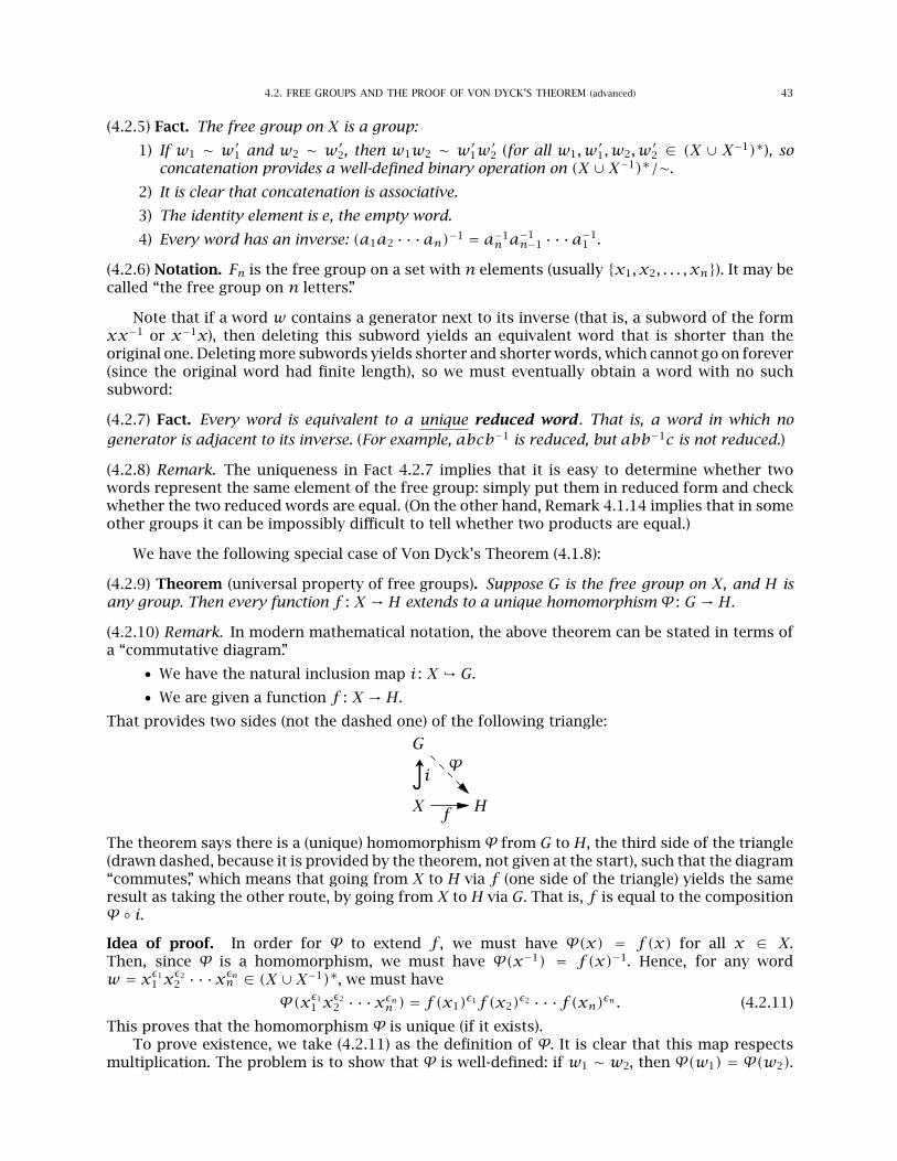
4.2. FREE GROUPS AND THE PROOF OF VON DYCK’S THEOREM (advanced) 43
(4.2.5) Fact. The free group on X is a group:
1) If w1 ∼ w′1 and w2 ∼ w′
2, then w1w2 ∼ w′1w′
2 (for all w1,w′1,w2,w′
2 ∈ (X ∪ X−1)∗), soconcatenation provides a well-defined binary operation on (X ∪X−1)∗/∼.
2) It is clear that concatenation is associative.
3) The identity element is e, the empty word.
4) Every word has an inverse: (a1a2 · · ·an)−1 = a−1n a
−1n−1 · · ·a−1
1 .
(4.2.6) Notation. Fn is the free group on a set with n elements (usually {x1, x2, . . . , xn}). It may becalled “the free group on n letters.”
Note that if a word w contains a generator next to its inverse (that is, a subword of the formxx−1 or x−1x), then deleting this subword yields an equivalent word that is shorter than theoriginal one. Deleting more subwords yields shorter and shorter words, which cannot go on forever(since the original word had finite length), so we must eventually obtain a word with no suchsubword:
(4.2.7) Fact. Every word is equivalent to a unique reduced word . That is, a word in which nogenerator is adjacent to its inverse. (For example, abcb−1 is reduced, but abb−1c is not reduced.)
(4.2.8) Remark. The uniqueness in Fact 4.2.7 implies that it is easy to determine whether twowords represent the same element of the free group: simply put them in reduced form and checkwhether the two reduced words are equal. (On the other hand, Remark 4.1.14 implies that in someother groups it can be impossibly difficult to tell whether two products are equal.)
We have the following special case of Von Dyck’s Theorem (4.1.8):
(4.2.9) Theorem (universal property of free groups). Suppose G is the free group on X, and H isany group. Then every function f : X → H extends to a unique homomorphism φ : G → H.
(4.2.10) Remark. In modern mathematical notation, the above theorem can be stated in terms ofa “commutative diagram.”
• We have the natural inclusion map i : X ↩ G.
• We are given a function f : X → H.
That provides two sides (not the dashed one) of the following triangle:
G
X H
i
f
φ
↪→
The theorem says there is a (unique) homomorphismφ from G to H, the third side of the triangle(drawn dashed, because it is provided by the theorem, not given at the start), such that the diagram“commutes,” which means that going from X to H via f (one side of the triangle) yields the sameresult as taking the other route, by going from X to H via G. That is, f is equal to the compositionφ ◦ i.Idea of proof. In order for φ to extend f , we must have φ(x) = f(x) for all x ∈ X.Then, since φ is a homomorphism, we must have φ(x−1) = f(x)−1. Hence, for any wordw = xϵ1
1 xϵ22 · · ·xϵnn ∈ (X ∪X−1)∗, we must have
φ(xϵ11 x
ϵ22 · · ·xϵnn ) = f(x1)ϵ1f(x2)ϵ2 · · ·f(xn)ϵn . (4.2.11)
This proves that the homomorphism φ is unique (if it exists).To prove existence, we take (4.2.11) as the definition of φ. It is clear that this map respects
multiplication. The problem is to show that φ is well-defined: if w1 ∼ w2, then φ(w1) = φ(w2).
44 4. CONSTRUCTIONS OF GROUPS
The formal proof requires some care, but the idea is easy enough:φ(x1x2 · · ·xkaa−1y1y2 · · ·yℓ)
= f(x1)f (x2) · · ·f(xk) f (a)f(a)−1 f(y1)f (y2) · · ·f(yℓ)= f(x1)f (x2 · · ·f(xk)f (y1)f (y2) · · ·f(yℓ)=φ(x1x2 · · ·xky1y2 · · ·yℓ). □
(4.2.12) Corollary. Every group is a homomorphic image of a free group.
Proof. LetX be any set that generatesG, and let F be the free group onX. Then the inclusionX ↩ Gextends to a homomorphismφ : F → G. Sinceφ(F) containsφ(X) = f(X) = X, which generatesG,we must have φ(F) = G. So φ is a homomorphism from F onto G, so G is a homomorphic imageof F. □
Here is another way of saying the same thing:
(4.2.13) Corollary. Every group is (isomorphic to) a quotient of a free group. In other words, everygroup is isomorphic to F/N, for some free group F and some normal subgroup N of F.
This observation is the foundation of the formal definition of a group defined by generatorsand relations.
(4.2.14) Example. To construct the group G = ⟨a,b | ab = b−1a ⟩, we first let F be the free groupon {a,b}. Then F has the correct generators, but does not have the necessary relation betweena and b. To impose this relation, we pass to a quotient group in which the relation does hold.Namely, if we rewrite the desired relation as aba−1b = 1 (by moving all terms to the left-handside), then we see that we are looking for a quotient F/N of F in which aba−1b is trivial. Thismeans that we need to have aba−1b ∈ N.
However, we want to make sure that the group F/N does not satisfy any relations that arenot consequences of the required relation aba−1b = 1. That means that we do not want to makeanything equal to the identity if it does not have to be equal to the identity: we want as fewelements of F to be trivial as possible. So N should be as small as possible. Hence, we let N be thesmallest normal subgroup of F that contains aba−1b. (Since the intersection of normal subgroupsis a normal subgroup, this smallest normal subgroup is unique.)
The same idea works in general, and yields the following official construction of a groupdefined by generators and relations.
(4.2.15) Definition. Suppose X is a set, and {w1, v1, . . . , vn, vn} is a set of words in (X ∪ X−1)∗.Then
⟨X | w1 = v1, . . . ,wn = vn ⟩ = F/N,where
• F is the free group on X, and
• N is the (unique) smallest normal subgroup of F that contains wiv−1i for all i.
(4.2.16) Exercise. Use Definition 4.2.15 (and the Correspondence Theorem) to provide a shortproof of Von Dyck’s Theorem (4.1.8).
§4.3. Semidirect products (optional)
(4.3.1) Recall.
1) If A and B are groups, then the Cartesian product A× B is a group under componentwisemultiplication: (a1, b1) · (a2, b2) = (a1a2, b1b2). This group is called the direct productof A and B.

4.3. SEMIDIRECT PRODUCTS (optional) 45
2) If A and B are normal subgroups of G, such that AB = G and A∩ B = {1}, then G ≊ A× B,and we say that G is the internal direct product of A and B (see Exercise 3.2.17).
If A and B are abelian, then A×B is abelian. This section describes an important generalizationof the direct product that often yields nonabelian groups, even when the factors A and B areabelian. The key is to remove the assumption that B is normal, while retaining the assumptionthat A is normal:
(4.3.2) Definition. If A and B are subgroups of G, such that
A ⊴ G, AB = G, and A∩ B = {1},then we say that G is the internal semidirect product of A and B.
If A, B, and G are as in Definition 4.3.2, then, since A is normalized by B, there is an actionof B on A by conjugation: ba = bab−1. Note that, for all a1, a2 ∈ A and b1, b2 ∈ B, we have
(a1b1)(a2b2) = a1(b1a2b−11 )b1b2 = a1
b1a2 b1 b2. (4.3.3)
Furthermore, if we let φb(a) = ba, then φb ∈ Aut(A). Indeed, φ is a homomorphism from B toAut(A). Conversely, any homomorphism from B to Aut(A) arises from a semidirect product:
(4.3.4) Definition. Assume A and B are groups.
1) Recall from Exercise 2.1.3 that an action of B on A is defined by any homomorphismφ : B → SA. We say that the action is by automorphisms if φb ∈ Aut(A), for all b ∈ B. (Inother words, if φ : B → Aut(A).) We usually write ba for φb(a).
2) For any action of B on A by automorphisms, we define a binary operation on A× B by:
(a1, b1)∗ (a2, b2) =(a1
b1a2, b1b2).
The resulting group is called the semidirect product of A and B, and is denoted A⋊ B.
(4.3.5) Remarks.
1) The binary operation in Definition 4.3.4(2) is based on the formula in (4.3.3).
2) If φ is the trivial homomorphism, then A⋊ B is the direct product A× B.
3) If the choice of the homomorphism φ is not clear from the context, it can be included inthe notation as a subscript: A⋊φ B.
4) The notation A⋊ B is used because it combines the symbol for a direct product (“×”) withthe symbol for a normal subgroup — the right half of ⋊ is ◁. This is intended to reflectthe fact that A is normal (“◁”) in A⋊ B.
(4.3.6) Exercises. Let G = A⋊ B, with respect to some action of B on A by automorphisms.
1) Verify that the binary operation ∗ in Definition 4.3.4 satisfies the group axioms.
2) Show:(a) A = { (a,1) | a ∈ A } is a subgroup of G that is isomorphic to A.(b) B = { (1, b) | b ∈ B } is a subgroup of G that is isomorphic to B.(c) G is the internal semidirect product of A and B.
(4.3.7) Exercises.
1) Show that the Klein bottle group ⟨x,y | yxy−1 = x−1 ⟩ is isomorphic to a semidirectproduct Z⋊ Z.
2) Show that the symmetric group S4 is the semidirect product of a group of order 4 and agroup of order 6.
(4.3.8) Exercises (contrast with Exercise 2.3.13(3)). Assume p and q are prime, with q ≡ 1 (mod p).
1) Show there is a nonabelian group of order pq.[Hint: Cauchy’s Theorem implies that Aut(Zq) has a subgroup P of order p. Then Zq ⋊P is a nonabelian group oforder pq.]
46 4. CONSTRUCTIONS OF GROUPS
2) Show that every group of order pq is the internal semidirect product of a subgroup oforder q and a subgroup of order p.
3) Show the group in (1) is unique (up to isomorphism).[Hint: You may assume (without proof) that Aut(Zq) is cyclic, and therefore has a unique subgroup of order p.]
(4.3.9) Exercise. Recall that a natural number is square-free if no divisor of the number (otherthan 1) is a perfect square.
It is known that every group of square-free order is solvable. Assuming this, show that everygroup of square-free order is the semidirect product of two cyclic groups.[Hint: Use Example 3.4.6 to show that G′′ is trivial. Every abelian group of square-free order is cyclic.]
Part II
Rings andModules

Chapter 5
Summary ofundergraduate ring theory
(5.0.1) Notation. R is always a ring (with 1).
§5.1. Elementary facts and definitions
(5.1.1) Definition. A ring is a set R together with two operations, called addition (+) andmultiplication (·), such that:
1) (R,+) is an (additive) abelian group, with identity element 0.
2) There exists a multiplicative identity element. This means there exists 1 ∈ R, such that1 · r = r · 1 = r for all r ∈ R.
3) Multiplication is associative. This means r(st) = (rs)t for all r , s, t ∈ R.
4) The distributive laws hold. More precisely, multiplication distributes over addition, bothon the left and on the right. This means r(s + t) = rs + rt and (r + s)t = rt + st for allr , s, t ∈ R.
(5.1.2) Warning. Any two elements of a ring can be added, subtracted, or multiplied, but there isno requirement that they can be divided (even if they are nonzero). For example, Z is a ring, butthe quotient of two elements of Z is usually not in Z.
(5.1.3) Other conventions. Some textbooks do not require rings to have a multiplicative identityelement, so they omit (2) from the definition.
(5.1.4) Example. Some rings to keep in mind are:
1) Z = {. . . ,−3,−2,−1,0,1,2,3, . . .},2) Zn = {0,1,2, . . . , n− 1},3) polynomial rings, such as R[x], C[x], Z[x], and Zn[x] (see Definition 5.5.2), and
4) the ring Matn×n(C) of n×nmatrices with entries in C.
(5.1.5) Exercises. Let r , s, and t be elements of R. Prove the following facts from middle-schoolalgebra:
1) r · 0 = 0 · r = 0,
2) (−1) · r = r · (−1) = −r ,
3) (−r) · s = r · (−s) = −rs,4) (−r)(−s) = rs,5) r(s − t) = rs − rt and (r − s)t = rt − st.
49
50 5. SUMMARY OF UNDERGRADUATE RING THEORY
(5.1.6) Warning. In elementary school, you are taught that if rs = 0, then either r = 0 or s = 0.This is not always true for a general ring. (For example, 2 · 3 = 0 in Z6.)
(5.1.7) Definition (ideals).
1) A nonempty subset I of R is a left ideal if it is closed under addition and is also closedunder multiplication on the left by elements of R. This means that• i1 + i2 ∈ I for all i1, i2 ∈ I, and• ri ∈ I, for all r ∈ R and i ∈ I.
2) Similarly, a nonempty subset I of R is a right ideal if it is closed under addition and closedunder multiplication on the right by elements of R.
3) A subset of R that is both a left ideal and a right ideal is called an ideal (or, for emphasis,it can be called a two-sided ideal). We write I ⊴ R to denote that I is a two-sided ideal of R.
4) The obvious (two-sided) ideals of R are {0} and R. We call {0} the zero ideal. (All otherideals are nonzero.) A (right or left or two-sided) ideal I of R is said to be proper if I ≠ R.
5) If I is a two-sided ideal of R, then the quotient ring R/I is the ring whose elements are theadditive cosets r + I of I (with r ∈ R) with addition and multiplication defined by:• (r1 + I)+ (r2 + I) = (r1 + r2)+ I, and• (r1 + I)(r2 + I) = r1r2 + I.
(5.1.8) Exercises.
1) Show that if I and J are (left or right or two-sided) ideals of R, then I ∩ J is a (left or rightor two-sided) ideal of R.
2) Show that the intersection of any number of (left or right or two-sided) ideals of R is a (leftor right or two-sided) ideal of R.
3) Show that if I and J are (left or right or two-sided) ideals of R, then I + J is a (left or rightor two-sided) ideal of R.
4) For any x ∈ R, show that the set Rx = { rx | r ∈ R } is the smallest left ideal thatcontains x. (Similarly, xR = {xr | r ∈ R } is the smallest right ideal that contains x.)
(5.1.9) Basic facts (commutative rings).
1) A ring R is commutative if rs = sr for all r , s ∈ R.
2) The rings Z, Zn, R[x], C[x], Z[x], and Zn[x] are commutative.
3) If n > 1, then Matn×n(C) is not commutative. For example, we have[0 10 0
][0 01 0
]=[
1 00 0
]≠
[0 00 1
]=[
0 01 0
][0 10 0
].
4) In a commutative ring, there is no difference between left ideals and right ideals — all ofthem are two-sided.
5) Quotients of commutative rings are commutative: if R is a commutative ring, and I is anideal of R, then R/I is commutative.
(5.1.10) Basic facts. Let R be a ring.
1) A subset S of R is a subring if it is a ring under the operations obtained by restricting theoperations of G. Equivalently: 1 ∈ S and, for all s1, s2, s ∈ S, we have s1+ s2 ∈ S, s1 · s2 ∈ S,and −s ∈ S
2) A subring S of R is said to be proper if S ≠ R.
3) Every subring of a commutative ring is commutative.
4) The intersection of any number of subrings of R is a subring of R.
5) The direct sum of two rings R and S is denoted R ⊕ S. This is the ring whose elementsare the elements of the Cartesian product R × S, with addition and multiplication definedcomponentwise: (r1, s2)+ (r2, s2) = (r1 + s1, r2 + s2) and (r1, s2) · (r2, s2) = (r1s1, r2s2).
5.2. HOMOMORPHISMS AND ISOMORPHISMS 51
6) Direct sums of commutative rings are commutative: if R and S are commutative rings, thenR ⊕ S is commutative.
(5.1.11) Exercise. Fix some n ∈ Z, and let
Z[√n] = {a+ b√n | a,b ∈ Z }.
1) Show that Z[√n]
is a subring of C.2) Show that if d ≥ 0, then Z
[√n]
is a subring of R.
§5.2. Homomorphisms and isomorphisms
(5.2.1) Definition. Assume R and S are rings.1) A function φ : R → S is a (ring) homomorphism if it respects the ring operations. That is,
we haveφ(r1 + r2) =φ(r1)+φ(r2), φ(r1r2) =φ(r1) ·φ(r2), and φ(1R) = 1S
for all r1, r2 ∈ R. (Here, to avoid confusion, we have used 1R to denote the multiplicativeidentity element of R, and 1S to denote the multiplicative identity element of S.)
2) A bijective homomorphism is called an isomorphism.3) We say that R and S are isomorphic (and write R ≊ S) if there is an isomorphism from R
to S. This is an equivalence relation:
R ≊ R, R ≊ S ⇒ S ≊ R, and R ≊ S ≊ T ⇒ R ≊ T .
4) kerφ =φ−1(0S) = { r ∈ R |φ(r) = 0S } is called the kernel of φ.5) An isomorphism from R to itself is called an automorphism of R.
(5.2.2) Exercises. Assume φ is a homomorphism from R to S. Prove the following basic facts.
1) The inverse of an isomorphism is an isomorphism: if φ is an isomorphism, thenφ−1 is anisomorphism from S to R.
2) Homomorphisms respect multiples and powers: we haveφ(kr) = kφ(r) and φ(r ℓ) =φ(r)ℓ
for r ∈ R, k ∈ Z, and ℓ ∈ Z+. (Also, φ(0R) = 0S.)3) If T is a subring of R, then φ(T) is a subring of S.4) φ is one-to-one if and only if kerφ = {0}.5) kerφ is a two-sided ideal of R.6) Conversely, if I is any two-sided ideal of R, then the function φ(x) = x + I is a
homomorphism from R to R/I whose kernel is I.
Isomorphisms preserve all properties that can be expressed in ring-theoretic terms. Forexample:
(5.2.3) Examples. Assume φ : R ≊-→ S, and let r , r ′ ∈ R. Then:
1) r commutes with r ′ if and only if φ(r) commutes with φ(r ′).2) R is commutative if and only if S is commutative.3) every left ideal of R is a two-sided ideal if and only if every left ideal of S is a two-sided
ideal.4) R has a nonzero, proper ideal if and only if S has a nonzero, proper ideal.5) R is a PID (or UFD, or Euclidean domain) if and only if S is a PID (or UFD, or Euclidean
domain) (see Definition 5.3.2).6) etc.
Although fundamental, the material in the remainder of this section is optional, because noneof it will be needed in later chapters.
52 5. SUMMARY OF UNDERGRADUATE RING THEORY
(5.2.4) Proposition (1st, 2nd, and 3rd Isomorphism Theorems).
1) If φ is a homomorphism from R to S, then R/kerφ ≊φ(R).More precisely, an isomorphism φ : R/kerφ → φ(R) can be obtained by defining
φ(r + kerφ) =φ(r).2) Suppose I ⊴ R and S is a subring of R. Then
(a) S + I is a subring of R (where S + I = { s + i | s ∈ S, i ∈ I }),(b) S ∩ I is an ideal of S, and(c) (S + I)/I ≊ S/(S ∩ I).
3) Suppose I and J are ideals ofR, with I ⊆ J. Then J/I is an ideal ofR/I, and (R/I)/(J/I) ≊ R/J.(5.2.5) Proposition (Correspondence Theorem). Suppose I is a two-sided ideal of R.
1) There is a one-to-one correspondence between the subrings of R that contain I and thesubrings of R/I. Namely, the subring of R/I corresponding to a subring S of R is S/I.
2) There is a one-to-one correspondence between the (right, left, or two-sided) ideals of Rthat contain I and the (right, left, or two-sided) ideals of R/I. Namely, the ideal of R/Icorresponding to an ideal J of R is J/I.
§5.3. PIDs, UFDs, and Euclidean domains
After giving the necessary definitions, this section proves that
Euclidean5.3.5=⇒ PID
5.3.11=⇒ UFD.
(5.3.1) Assumption. The ring R is commutative.
(5.3.2) Definitions.
1) An element r of R is a zero divisor if r ≠ 0 and there exists s ∈ R ∖ {0}, such that rs = 0.
2) R is an integral domain if it does not have any zero divisors.
3) R is a Euclidean domain if(a) R is an integral domain, and(b) there is a function d : R → N, such that
• d(r) = 0 ⇐⇒ r = 0, and• for all a,b ∈ R with b ≠ 0, there exists q, r ∈ R with a = bq+r and d(r) < d(b).
(The natural number d(r) is often called the norm of the element r .)
4) An ideal I of R is principal if I = Rr , for some r ∈ R.
5) R is a principal ideal domain (or PID, for short) if(a) R is an integral domain, and(b) every ideal of R is principal.
6) An element u of R is a unit if it has a multiplicative inverse (that is, there exists r ∈ R,such that ur = 1).
7) Two nonzero elements r and s are associates if r = us, for some unit u. (So the associatesof 1 are precisely the units.) This is an equivalence relation.
8) We write r | s to mean that r is a divisor of s (that is, there exists t ∈ R with rt = s).9) A nonzero element π of R is irreducible if it is not a unit, and every divisor of π is either
a unit or an associate of π.
10) R is a unique factorization domain (or UFD, for short) if every nonzero nonunit of R canbe written uniquely as a product of irreducibles (up to associates and a permutation of thefactors). More precisely, for every r ∈ R, such that r ≠ 0 and r is not a unit:(a) there exist irreducibles π1, π2, . . . , πk, for some k, such that r = π1, π2, . . . , πk, and(b) if r = π ′1, π ′2, . . . , π ′ℓ, where π ′1, π ′2, . . . , π ′ℓ are irreducible, then k = ℓ, and there existsσ ∈ Sk, such that πi is an associate of π ′σ(i) for all i.
5.3. PIDS, UFDS, AND EUCLIDEAN DOMAINS 53
11) A nonzero element p of R is prime if it is not a unit and, for all r , s ∈ Rwith p | rs, we haveeither p | r or p | s. (Note that every prime element of an integral domain is irreducible,and that the converse is true in any UFD.)
12) The zero ring is the ring with only one element. Any ring with more than one element isa nonzero ring.
13) If F is a nonzero commutative ring, and every nonzero element of F is a unit, then we saythat F is a field .
(5.3.3) Examples. For our purposes, the two most important examples of Euclidean domains are:1) Z is a Euclidean domain: let d(n) = |n|.2) If F is any field, then we will see in Section 5.5 that the polynomial ring F[x] is a Euclidean
domain, with d(f(x)
) = 1+ deg f(x) (except that d(0) = 0).
We require the following basic fact:
(5.3.4) Exercise. Show that N is well-ordered . (This means that every nonempty subset of N hasa smallest element.)[Hint: Prove by induction on n: If S is a subset of N that contains an element ≤ n, then S has a smallest element.]
(5.3.5) Proposition. Every Euclidean domain is a PID.
Proof. Let I be any ideal of R. Since {0} = R0 is principal, we may assume I ≠ {0}. Then{d(i) | i ∈ I ∖ {0} } is a nonempty subset of Z+, so it has a smallest element (because N is well-ordered; see Exercise 5.3.4). Hence, we may choose some i0 ∈ I, such that
d(i0) ≤ d(i) for all nonzero i ∈ I. (5.3.6)
We claim that I = Ri0. To see this, let i be an arbitrary element of I. Since R is Euclidean,there exist q, r ∈ R, such that i = qi0 + r , and d(r) < d(i0). Now r = i − qi0 ∈ I − RI ⊆ I,so we have r ∈ I and d(r) < d(i0). Therefore, the minimality of d(i0) implies r = 0. Soi = qi0 + r = qi0 + 0 = qi0 ∈ Ri0. Since i is an arbitrary element of I, this implies I ⊆ Ri0.The opposite inclusion is obvious, because i0 ∈ I and I is an ideal. □
(5.3.7) Example. The fact that every Euclidean domain is a PID provides us with two importantexamples of PIDs:
• Z is a PID.• If F is any field, then the polynomial ring F[x] is a PID.
In Chapter 7, we will study the structure of “modules” over any PID, but these two rings are themost important examples.
Our proof that every PID is a UFD relies on the following important notion:
(5.3.8) Definition. R has the ascending chain condition (or acc , for short) if it satisfies any of thefollowing equivalent conditions:
1) Every ascending chain of ideals is eventually constant. That is,if I1 ⊆ I2 ⊆ · · · is any ascending chain of ideals,then there is some n, such that In = In+1 = In+2 = · · · .
2) There is no infinitely long strictly increasing chain of ideals. That is,there do not exist ideals I1, I2, . . ., such that I1 ⊊ I2 ⊊ I3 ⊊ · · · .
3) Every ideal is finitely generated. That is, if I is any ideal, then there exist x1, x2, . . . , xn ∈ R(for some n) such that I = ⟨x1, . . . , xn⟩ is the ideal generated by x1, x2, . . . , xn.
4) Every nonempty set ( of ideals has a maximal element. That is, there is some M ∈ (, suchthat there does not exist I ∈ ( with M ⊊ I.
(Alternate terminology: saying that R is Noetherian is the same as saying that R has the acc.)
(5.3.9) Exercises. Assume R is an integral domain.
54 5. SUMMARY OF UNDERGRADUATE RING THEORY
1) Show that if I1 ⊆ I2 ⊆ I3 ⊆ · · · is an increasing chain of ideals, then⋃∞n=1 In is an ideal.
2) It is fairly obvious that the first two formulations in Definition 5.3.8 are equivalent.(a) Show that 5.3.8(3) is equivalent to 5.3.8(2).
[Hint: (⇐) If I1 ⊊ I2 ⊊ I3 ⊊ · · · , then⋃n In is an ideal that is not finitely generated (because any finite
subset of I is contained in some In). (⇒) If I is not finitely generated, then a sequence {x1, x2, . . .} can beconstructed by induction, such that xn+1 ∉ ⟨x1, . . . , xn⟩ =: In.]
(b) Show that 5.3.8(4) is equivalent to 5.3.8(2).[Hint: (⇒) If ( has no maximal element, you can inductively construct a strictly increasing chain of idealsin (. (⇐) If {In} is a strictly increasing chain of ideals, then it has no maximal element.]
3) For r , s ∈ R, show that if Rrs = Rr , then either r = 0 or s is a unit.
4) Assume R has the acc. Show that if r is any element of R that is not a unit, then r is divisibleby some irreducible.[Hint: Suppose r0 is not divisible by any irreducible. By induction, construct a sequences {rn}n≥0 and {sn}n≥1,such that rn = rn+1sn+1, and neither rn nor sn is a unit. Then Rr0 ⊊ Rr1 ⊊ Rr2 · · · .]
5) Show that if R has the acc, then every nonzero, non-unit element of R is the product offinitely many irreducibles.[Hint: Suppose r0 is not the product of finitely many irreducibles. Use Exercise 5.3.9(4) to inductively constructsequences {πn}n≥1 and {rn}n≥0, such that rn = πn+1rn+1. Then Rr0 ⊊ Rr1 ⊊ Rr2 · · · .]
6) A ring has the descending chain condition (or dcc , for short) if every descending chain ofideals is eventually constant. Show that a nonzero integral domain with the dcc must be afield.[Hint: Given r ∈ R, you need to show that r has a multiplicative inverse. Consider the ideals Rr,Rr2, Rr3, . . ..]
We now know that every element of a ring with the acc is a product of irreducibles. Thefollowing result is the key to proving that the product is unique when the ring is a PID.
(5.3.10) Lemma. If R is a PID, then every irreducible element of R is prime.
Proof. Assume π, r1, r2 ∈ R, such that π is irreducible, and neither r1 nor r2 is divisible by π. Foreach i, since R is a PID, we have ⟨ri, π⟩ = Rdi some di ∈ R. Then π ∈ Rdi, so di | π. Since π isirreducible, this implies that we may assume (after multiplying by a unit) that di is either 1 or π.However, since π ∤ ri, we have ri ∉ Rπ, so di ≠ π. Therefore di = 1, which means ⟨ri, π⟩ = R.Hence, there exist ai, bi ∈ R, such that airi + biπ = 1, so airi ≡ 1 (mod π). Then
(r1r2)a1a2 = (a1r1)(a2r2) ≡ 1 · 1 = 1 ≡ 0 (mod π),so r1r2 ≡ 0 (mod π). □
(5.3.11) Proposition. Every PID is a UFD.
Proof. We already saw in Exercise 5.3.9(5) that every nonzero non-unit in R is a product ofirreducibles, so all that remains to prove is uniqueness.
Suppose π1 · · ·πk = uπ ′1 · · ·π ′ℓ, where every πi and π ′j is irreducible, and u is a unit. Theleft-hand side is obviously divisible by πk, so the right-hand side must also be divisible by πk.From Lemma 5.3.10 (and induction), this implies that some π ′j is divisible by πk. By permuting thefactors on the right-hand side, we may assume it is π ′ℓ that is divisible by πk. Since π ′ℓ and πk areirreducible, this implies that they are associates, so π ′ℓ = u′πk, for some unit u′. Then we have
π1 · · ·πk = uπ ′1 · · ·π ′ℓ = uπ ′1 · · ·π ′ℓ−1(u′πk) = uu′π ′1 · · ·π ′ℓ−1πk,
so π1 · · ·πk−1 = uu′π ′1 · · ·π ′ℓ−1. Then, by induction on k, we must have k− 1 = ℓ− 1 (so k = ℓ),and there exists σ ∈ Sk−1, such that πi is an associate of π ′σ(i) for all i. □
(5.3.12) Exercises.
1) Suppose r , s ∈ R. We say that d is a greatest common divisor (or gcd for short) of r and sif• d is a common divisor of r and s (that is, we have d | a and d | s),
5.4. RINGS IN NUMBER THEORY (optional) 55
• every common divisor of r and s is a divisor of d.Show that if R is a UFD, then any two elements of R have a greatest common divisor, andthat the gcd is unique up to multiplying by a unit.
2) More generally, show that if R is a UFD, then any finite set {r1, r2, . . . , rk} of elements of Rhas a greatest common divisor (which is unique up to multiplying by a unit).
3) Assume that R is a UFD, and let d = gcd(r1, . . . , rk), where r1, . . . , rk ∈ R. Show thatgcd(r1/d, r2/d, . . . , rk/d) = 1.
4) Assume R is a PID. Then R is a UFD, so any two elements have a gcd. Show:(a) ⟨r , s⟩ = ⟨gcd(r , s)⟩.(b) There exist a,b ∈ R, such that ar + bs = gcd(r , s).
5) Assume R is a PID, and r ∈ R ∖ {0}. Show the ideal ⟨r⟩ is maximal if and only if r isirreducible. (An ideal I of R is maximal if it is a proper ideal, and there does not exist anideal J, such that I ⊊ J ⊊ R.)
6) Assume that R is a UFD, and that there exist infinite sequences r0, r1, r2, . . . and s0, s1, s2, . . .of distinct elements of R, such that risi = r0s0 for all i. Show that R has infinitely manyunits.
§5.4. Rings in number theory (optional)
Finding integer solutions of polynomial equations is a fundamental problem in the branch ofmathematics that is called “number theory.” For example, we might want to find solutions of theequation x2 − 2y2 = 1. (Only integer solutions are allowed: x and y are required to be elementsof Z.) One solution can be obtained by letting x = 1 and y = 0, but we will use ring theory to seethat there are infinitely many other solutions. This is an illustration of the branch of mathematicsthat is called “algebraic number theory.”
Instead of only looking at the single equation x2 − 2y2 = 1, we will allow the coefficient 2 tobe replaced with any integer:
(5.4.1) Problem. For each n ∈ Z, determine whether the “Pell Equation” x2−ny2 = 1 has infinitelymany integer solutions.
Two cases are too easy to be interesting:
(5.4.2) Exercises.
1) Assume n is a perfect square. (This means that n = k2, for some k ∈ Z.) Show that theequation x2 −ny2 = 1 has infinitely many integer solutions if and only if n = 0.[Hint: x2 −ny2 = (x − ky)(x + ky).]
2) Assume n < 0. Show that the equation x2 − ny2 = 1 has only finitely many integersolutions.[Hint: If x2 −ny2 = 1, then x2 ∈ {0,1} and −ny2 ∈ {0,1}, because x2 ≥ 0 and −ny2 ≥ 0.]
The remainder of this section will provide a proof of the following answer to the remainingcases:
(5.4.3) Theorem. Ifn is a positive integer that is not a perfect square, then the equationx2−ny2 = 1has infinitely many integer solutions.
Henceforth, we will always ignore the trivial cases:
(5.4.4) Assumption. n is a positive integer that is not a perfect square.
To prove Theorem 5.4.3, we will first show that it is actually a problem in ring theory. Let’sstart with some basic facts. (Recall that the ring Z
[√n]
was introduced in Exercise 5.1.11.)
56 5. SUMMARY OF UNDERGRADUATE RING THEORY
(5.4.5) Exercises.
1) Show that√n is irrational.
[Hint: If√n = r/s, with r , s ∈ Z, then ns2 = r2. In the prime factorization of the right-hand side, each prime
appears an even number of times, so the same must be true on the left-hand side. Therefore, each prime factorof n appears an even number of times, which means that n is a perfect square.]
2) For a1, a2, b1, b2 ∈ Z, we have a1 + b1√n = a2 + b2
√n if and only if a1 = a2 and b1 = b2.
[Hint: Use Exercise 1.]
3) Define : Z[√n]→ Z
[√n]
by a+ b√n = a− b√n. (Exercise 2 implies that this function iswell-defined.) Show that this is an automorphism of Z
[√n]. This is called the conjugation
automorphism of Z[√n].
4) Define N : Z[√n] → Z by N(a + b√n) = a2 − nb2. (This is called the norm of a + b√n.)
Show:(a) N(r) = r r for all r ∈ Z[√n].(b) N respects multiplication: N(rs) = N(r)N(s) for all r , s ∈ Z[√n].
5) Assume n is odd and n < 0. Show that Z[√n]
is not a UFD.[Hint: Let r = 1 + √n and m = (1 − n)/2. Then 1 − n = r r = 2m. If the prime factorization is unique, then 2cannot be prime. This implies there is some x ∈ Z[√n] with N(x) = ±2.]
6) Assume n is odd and n > 0. Show that if Z[√n]
is a UFD, then there exists x ∈ Z, such thatx2 ≡ ±2 (mod n).[Hint: See the hint for Exercise 5.]
7) Show that Z[√n]
is not a UFD, for: (a) n = 5, (b) n = 13, (c) n = 15, (d) n = 21, (e) n = 25.[Hint: Exercise 6.]
(5.4.6) Lemma. An element r of Z[√n]
is a unit if and only if N(r) = ±1.
Proof. (⇐) We have r r = N(r) = ±1, so r has a multiplicative inverse (namely, either r or −r), sor is a unit.
(⇒) Let u be a multiplicative inverse of r . Then
1 = N(1) = N(ru) = N(r)N(u).Since N(r) and N(u) are integers, this implies N(r) ∈ {±1}. □
We can now translate Theorem 5.4.3 into ring theory:
(5.4.7) Exercise. The equation x2 − ny2 = 1 has infinitely many solutions if and only if the ringZ[√n]
has infinitely many units.[Hint: (⇒) If x2 −ny2 = 1, then x +y√n is a unit.
(⇐) If v is a unit such that N(v) = −1, then we have either N(u) = 1 or N(uv) = 1, for every unit u.]
Thus, we wish to show that Z[√n]
has infinitely many units. The proof will use the followingfact:
(5.4.8) Exercise. For every integer k > 0, show there exist nonzero a,b ∈ Z, such that 1 ≤ b ≤ kand
∣∣a− b√n∣∣ ≤ 1/k.[Hint: For x ∈ R, let ((x)) = x − ⌊x⌋ be the fractional part of x, where ⌊x⌋ is the greatest integer that is ≤ x. Then
((0)), ((−√n)), ((−2√n)), . . . ((−k√n))
is a list of k+ 1 numbers that are between 0 and 1, so there must be two of them whose difference is less than 1/k.]
Now, we can prove the ring-theoretic version of Theorem 5.4.3:
(5.4.9) Theorem. If n is a positive integer that is not a perfect square, then the ring Z[√n]
hasinfinitely many units.
Proof. For each k ∈ Z+, Exercise 5.4.8 provides nonzero a,b ∈ Z, such that |b| ≤ k and∣∣a+ b√n∣∣ ≤ 1/k. Then|a| ≤ |b|√n+ 1/k ≤ k√n+ 1,
5.5. FIELDS AND POLYNOMIALS 57
so ∣∣a+ b√n∣∣ = ∣∣a− b√n∣∣ ≤ (k√n+ 1)+ k√n = 2k√n+ 1.
Therefore ∣∣N(a+ b√n)∣∣ = ∣∣(a+ b√n)(a+ b√n)∣∣≤ 1k· (2k√n+ 1
)≤ 2
√n+ 1.
By choosing infinitely many different values for k, we see that there are infinitely manydifferent elements r of Z
[√n], such that |N(r)| ≤ 2
√n + 1 (see Exercise 5.4.10). Since there
are only finitely many possibilities for N(a + b√n), we conclude that there are infinitely many
elements r0, r1, r2, . . . of Z[√n], such that N(ri) = N(r0) for all i. (Remark: If Z
[√n]
is a UFD,then applying Exercise 5.3.12(6) completes the proof without need for any further explanation.)Furthermore, since there are only finitely many congruence classes moduloN(r0), we may assumethat ri ≡ r0 (mod N(r0)) for all i. This means that
ri − r0
N(r0)∈ Z[√n].
Now, for all i, we haverir0= ri r0
N(r0)= (ri − r0)r0
N(r0)+ r0 r0
N(r0)= (ri − r0)
N(r0)r0 + 1 ∈ Z[√n]
and
N(ri/r0) = N(ri)/N(r0) = N(r0)/N(r0) = 1,
so {r1/r0, r2/r0, r3/r0, . . .} is a set of infinitely many units. □
(5.4.10) Exercise. In the notation of the proof of Theorem 5.4.9, show there are infinitely manydifferent nonzero elements r of Z
[√n], such that |N(r)| ≤ 2
√n+ 1.
[Hint: If there are only finitely many, then there exists k so large that |r | > 1/k for all of them.]
§5.5. Fields and polynomials
(5.5.1) Exercise.
1) Show that a nonzero commutative ring is a field if and only if it has no nonzero, properideals.
2) Show that a ring R is the zero ring if and only if 0R = 1R.
(5.5.2) Definition (polynomials). Assume F is a field.
1) A polynomial over F is any expression of the form
anxn + an−1xn−1 + · · · + a1x + a0,where n ∈ N and each ai is an element of F.
2) Adding leading zeroes does not change a polynomial: if an+1 = an+2 = · · · = an+k, thenthe polynomial
∑n+ki=0 aixi is considered to be equal to the polynomial
∑ni=0 aixi.
3) We call∑ni=0 aixi the zero polynomial if ai = 0 for all i.
4) The degree of a polynomial f(x) = ∑ni=0 aixi is the largest value of i, such that ai ≠ 0.
(By convention, we may say that the degree of the zero polynomial is −1.) It is denoted bydeg f(x). Note that deg f(x) ≥ 0 if f(x) is not the zero polynomial.
5) A linear polynomial is a polynomial of degree 1.
58 5. SUMMARY OF UNDERGRADUATE RING THEORY
6) The set of all polynomials over F is a commutative ring. It is called the ring of polynomialsover F, and is denoted F[x]. Addition and multiplication of polynomials are defined justas in high school. Namely, if
f(x) =m∑i=0
aixi and g(x) =n∑i=0
bixi,
then
f(x)+ g(x) =max(m,n)∑i=0
(ai + bi)xi
and
f(x)g(x) =m+n∑i=0
cixi, where ck =k∑i=0
aibk−i
(and where we use the convention that ai = 0 for i > m and bi = 0 for i > n).
7) For f(x) =∑ni=0 aixi ∈ F[x] and c ∈ F, we let f(c) =∑ni=0 aici ∈ F. Note that the mappingf(x), f(c) is a ring homomorphism:• If f(x)+ g(x) = h(x), then f(c)+ g(c) = h(c).• If f(x)g(x) = h(x), then f(c)g(c) = h(c).
8) Let c ∈ F and f(x) ∈ F[x]. We say that c is a root (or zero) of f(x) if f(c) = 0.
(5.5.3) Exercise. Assume F is a field, and let f(x), g(x) ∈ F[x].1) Show that deg
(f(x)+ g(x)) ≤ max
(deg f(x),degg(x)
).
2) Show that if neither f(x) nor g(x) is the zero polynomial, then
deg(f(x)g(x)
) = deg f(x)+ degg(x).Conclude that f(x)g(x) is not the zero polynomial.
Polynomials can be defined over any ring, not only fields, but the following important resultdoes not hold for most other rings:
(5.5.4) Theorem. If F is a field, then F[x] is a Euclidean domain.
More precisely, we may let d(f(x)
) = 1+ deg f(x). This is an immediate consequence of thefollowing result:
(5.5.5) Theorem (Division Algorithm for Polynomials). Let f(x), g(x) ∈ F[x], where F is a field. Ifg(x) is not the zero polynomial, then there exist unique polynomials q(x), r(x) ∈ F[x], such that
f(x) = g(x)q(x)+ r(x) and deg r(x) < degg(x).
Proof. We first prove the existence of q(x) and r(x). This is accomplished by induction ondeg f(x). For the base case, note that if deg f(x) < degg(x), then we may let q(x) = 0 andr(x) = f(x). Therefore, we now assume that deg f(x) > degg(x). (In particular, f(x) is not thezero polynomial.) Write f(x) =∑mi=0 aixi and g(x) =∑ni=0 bixi with am ≠ 0 and bn ≠ 0. Now, let
f ′(x) = f(x)− ambnxm−n g(x).
(It is important to note that am/bn ∈ F, since bn ≠ 0 and F is a field. So ambn x
m−n g(x) is theproduct of two polynomials, and is therefore in F[x], because m − n = deg f − degg > 0.) Notethat, since deg f(x) =m and
deg(ambnxm−n g(x)
)= deg
ambnxm−n + degg(x) = (m−n)+n =m,
5.5. FIELDS AND POLYNOMIALS 59
we have deg f ′(x) ≤m. However, we also haveambnxm−n g(x) = am
bnxm−n
(bnxn + (terms of degree < n)
)= ambnxm−n · bnxn + ambn
xm−n · (terms of degree < n))
= amxm + (terms of degree <m),so the leading term of am
bn xm−n g(x) exactly cancels the leading term of f(x). Therefore
deg f ′(x) < deg f(x), so, by our induction hypothesis, there exist q′(x), r(x) ∈ F[x], such that
f ′(x) = g(x)q′(x)+ r(x) and deg r ′(x) < degg(x).Now, let q(x) = am
bn xm−n + q′(x). Then
g(x)q(x)+ r(x) = g(x)(ambn xm−n + q′(x))+ r(x)= am
bn xm−n g(x)+ (g(x)q′(x)+ r(x))
= (f(x)− f ′(x))+ f ′(x)= f(x).
Now, to prove uniqueness, suppose that
f(x) = g(x)q(x)+ r(x) and f(x) = g(x)q′(x)+ r ′(x),with deg r(x),deg r ′(x) < degg(x). Then high-school algebra tells us
r(x)− r ′(x) = g(x)(q′(x)− q(x)). (5.5.6)
If q′(x) ≠ q(x), then q′(x) − q(x) is not the zero polynomial, so we see from Exercise 5.5.3(2)that
deg(r(x)− r ′(x)) = degg(x)+ deg
(q′(x)− q(x)) ≥ degg(x).
This is a contradiction, since
deg(r(x)− r ′(x)) ≤ max
(deg r(x),deg r ′(x)
)< degg(x).
So we must have q′(x) = q(x). Then q′(x) − q(x) = 0, so (5.5.6) implies r(x) = r ′(x). We nowknow that q′(x) = q(x) and r ′(x) = r(x), which establishes the desired uniqueness. □
Note that if the linear polynomial x− c is a factor of f(x) (that is, if there exists q(x) ∈ F[x],such that f(x) = (x − c)q(x)), then
f(c) = (c − c)q(c) = 0 · q(c) = 0,so c is a root of f(x). The converse is a consequence of the Division Algorithm:
(5.5.7) Corollary. Suppose c ∈ F and f(x) ∈ F[x], where F is a field. If c is a root of f(x), thenthere exists q(x) ∈ F[x], such that f(x) = (x − c)q(x).Proof. From the Division Algorithm (5.5.5), we know there exist q(x), r(x) ∈ F[x], such thatf(x) = (x − c)q(x) + r(x), and deg r(x) < deg(x − c). Since deg(x − c) = 1, this impliesdeg r(x) ∈ {0,−1}, so r(x) is some constant a. (If deg r(x) = −1, then a = 0.) This impliesr(t) = a for all t ∈ F, so, in particular, we have r(c) = a. Then
0 = f(c) = (c − c)q(c)+ r(c) = 0 · q(c)+ a = a.This implies r(x) = a = 0, so we conclude that r(x) is the zero polynomial. Therefore
f(x) = (x − c)q(x)+ r(x) = (x − c)q(x)+ 0 = (x − c)q(x). □
(5.5.8) Definition. Let c ∈ F and f(x) ∈ F[x], where F is a field. From Corollary 5.5.7, we knowthat c is a root of f(x) if and only if the linear polynomial x − c is a factor of f(x). We say thatc is a repeated root of f(x) if (x − c)2 is a factor of f(x).

Chapter 6
Modules over a ring
A vector space has objects, called vectors, that can be added and can be multiplied by scalars. In afirst course in linear algebra, the scalars are usually real numbers (or perhaps complex numbers).Certainly, the scalars come from a field. We will now study the situation in which scalars areallowed to come from any ring. However, the term “vector space" is reserved for cases where thescalars are from a field; the space is called a “module” when the vectors come from a more generalring.
§6.1. Definition and basic facts
(6.1.1) Definition. A (left) module over R (or, for short, an R-module) is an abelian group M(written additively), together with an operation of scalar multiplication R ×M → M that satisfiesthe following natural axioms for all r , s ∈ R and m,n ∈ M:
1) (distributivity) r(m+n) = rm+ rn and (r + s)m = rm+ sm.2) (associativity) r(sm) = (rs)m.3) (identity axiom) 1m =m (where 1 is the multiplicative identity element of R).
(6.1.2) Other conventions. In some situations, it is more natural to put the scalars on the right,instead of on the left (writing mr instead of rm). Then M is called a right R-module, and theaxioms are:
(m+n)r =mr +nr, m(r + s) =mr +ms, (mr)s =m(rs), m1 =m.(6.1.3) Exercises. Assume r ∈ R andm ∈ M. Let 0R and 0M be the additive identity elements of Rand M, respectively. Show:
1) r 0M = 0M2) 0Rm = 0M3) (−r)m = r(−m) = −(rm)4) If rm = 0M, and r is a unit in R (that is, if r has a multiplicative inverse), then m = 0M.
(6.1.4) Examples.1) If R = R (or more generally, if R is any field), then the R-modules are precisely the vector
spaces over R (that is, the vector spaces whose scalars are the elements of the field R).2) Every (additive) abelian group A is a Z-module. Namely, the axioms are satisfied by the
usual multiplication of an integer times an element of the group (such as 3a = a+ a+ aand −3a = −(a+ a+ a)).
3) R is an R-module under left multiplication. (That is, the scalar multiplication is the sameas the multiplication that is part of the structure of R as a ring.) This is often called theregular R-module.
61
62 6. MODULES OVER A RING
4) More generally, every left ideal of R is an R-module.
5) For any n ∈ Z+, let Rn be the set of all n-tuples with entries in R. This is an R-module underthe usual componentwise scalar multiplication of vectors: r(s1, . . . , sn) = (rs1, . . . r sn).
6) Let Matn×n(R) be the set of all n×nmatrices with entries in R. This is a ring with the usual(entrywise) addition and (row-times-column) multiplication of matrices. If we identify Rnwith the set Matn×1(R) of n-dimensional column vectors with entries in R, then matrixmultiplication provides Rn with the structure of a Matn×n(R)-module.
(6.1.5) Exercises.
1) AssumeM is an R-module, andφ : S → R is a ring homomorphism (withφ(1S) = 1R). Showthat M is an S-module, where the scalar multiplication is defined by s ·m =φ(s)m.
2) Suppose• V is a vector space over a field F, and• T : V → V is a linear transformation.
Show that V is an F[x]-module, where the scalar multiplication is defined by
f(x) · v =n∑i=0
ai T iv if f(x) =n∑i=0
aixi with ai ∈ F.
3) Find an example of an R-module M, such that we have rm = 0 for some r ∈ R ∖ {0} andm ∈ M∖{0}. (This complements Exercise 6.1.3(4) and demonstrates that not all propertiesof vector spaces remain true for modules.)[Hint: Take R = Z.]
§6.2. Submodules, quotients, homomorphisms, and annihilators
(6.2.1) Notation. In this section, M is always an R-module.
(6.2.2) Definitions.
1) A subset N ofM is a submodule ofM if N is an R-module under the same operations asM.Equivalently, N is not empty, and is closed under addition and scalar multiplication: forall n1, n2, n ∈ N and r ∈ R, we have
n1 +n2 ∈ N and rn ∈ N.We write N ≤ M to denote that N is a submodule of M.
2) The obvious submodules of M are {0} (the trivial submodule) and M. A submodule thatis not all of M is said to be a proper submodule of M.
3) Suppose N is a submodule of M. Then N is a subgroup of the additive group of M, so• we have the left coset m+N for each m ∈ M, and• M/N is the set of all left cosets of N.
It is straightforward to verify that M/N is a module, under the natural operations
(m1 +N)+ (m2 +N) = (m1 +m2)+M and r(m+N) = rm+N,for m1,m2,m ∈ M and r ∈ R. This is called the quotient of M by N.
(6.2.3) Remark. Unlike in group theory, where only the normal subgroups give rise to a quotientgroup, every submodule of M gives rise to a quotient module.
(6.2.4) Examples.
1) Considering R as an R-module under left-multiplication, the submodules of R are preciselythe left ideas of R.
2) If A is a Z-module, then the submodules of A are precisely the subgroups of A.
3) If R is a field, and V is a vector space over R, then the submodules of V are precisely thevector subspaces of V .
6.2. SUBMODULES, QUOTIENTS, HOMOMORPHISMS, AND ANNIHILATORS 63
(6.2.5) Exercises.
1) Assume N1,N2,N3 ≤ M. Show:(a) N1 +N2 ≤ M, where N1 +N2 = {n1 +n2 | n1 ∈ N1, n2 ∈ N2 }.(b) If N1 ⊆ N3, then (N1 +N2)∩N3 = N1 + (N2 ∩N3).
2) Assume s ∈ R, and R is commutative.(a) Show sM ≤ M, where sM = { sm |m ∈ M }.(b) Show {m ∈ M | sm = 0 } ≤ M.
3) Suppose I is a right ideal of R. Define
I⊥ = {m ∈ M | im = 0 for all i ∈ I }.Show I⊥ is a submodule of M.
Linear transformations are the maps between vector spaces that respect the operations ofaddition and scalar multiplication. For modules (as for groups, rings, and most other algebraicobjects), the maps that respect the operations are called homomorphisms:
(6.2.6) Definitions. Assume M and N are R-modules, and let φ : M → N.
1) φ is a homomorphism if φ(m1 +m2) = φ(m1) +φ(m2) and φ(rm) = r φ(m) for allm1,m2,m ∈ M and r ∈ R.
2) A bijective homomorphism is called an isomorphism.
3) We say thatM is isomorphic toN (and writeM ≊ N) if there exists an isomorphism fromMto N. It is straightforward to check that this is an equivalence relation.
4) If φ is a homomorphism, then:(a) kerφ = {m ∈ M |φ(m) = 0 }. This is the kernel of φ.(b) φ(M) = {φ(m) |m ∈ M }. This is the image of φ.
(6.2.7) Exercises. Assume φ : M → N is a homomorphism of R-modules.
1) Show that both the kernel and the image of φ are submodules. More precisely, showkerφ ≤ M and φ(M) ≤ N.
2) Show that the image of a submodule is a submodule: if M1 ≤ M, then φ(M1) ≤ N.
3) Show that the inverse image of a submodule is a submodule: if N1 ≤ N, thenφ−1(N1) ≤ M.
4) Show that the sum of two homomorphisms is a homomorphism: if ψ : M → N is anotherhomomorphism, then defining (φ+ψ)(m) =φ(m)+ψ(m)yields another homomorphismfrom M to N.
5) φ is one-to-one if and only if kerφ = {0}.(6.2.8) Exercise. Assume M is an R-module, and N ≤ M. Show that the natural map from M toM/N is a surjective homomorphism whose kernel is N.
(6.2.9) Exercise. Assume thatM is an R-module, and that R is a commutative. Show that each left-multiplication is a homomorphism fromM toM. More precisely, for each s ∈ R, defineφs : M → Mby φs(m) = sm, and show that φs is a homomorphism.
(6.2.10) Definitions. Assume M is an R-module.
1) For S ⊆ M, the (unique) smallest submodule of M that contains S is called the submodulegenerated by S, and is denoted ⟨S⟩.
2) If ⟨S⟩ = M, then we say that S is a generating set of M.
3) M is cyclic if it is generated by one-element subset: M = ⟨m⟩ for some m ∈ M.
4) For m ∈ M, the annihilator of m in R is AnnR(m) = { r ∈ R | rm = 0 }.5) The annihilator of M in R is
AnnR(M) = {r ∈ R | rm = 0 for allm ∈ M} = {r ∈ R | rM = 0} =⋂m∈M
AnnR(m).
64 6. MODULES OVER A RING
(6.2.11) Exercises. Assume M and N are R-modules.
1) Show ⟨m⟩ = Rm, for all m ∈ M.
2) More generally, show that if S = {s1, s2, . . . , sk} ⊆ M, then
⟨s1, s2, . . . , sk⟩ = Rs1 + Rs2 + · · · + Rsk.3) Assume {s1, s2, s3, . . . , sk} is a generating set ofM, andm = s1+q2s2+· · ·+qksk, for someq2, . . . , qk ∈ R. Show {m,s2, s3, . . . , sk} is also a generating set of M
4) Show AnnR(m) is a left ideal in R, for all m ∈ M.
5) Show AnnR(M) is a two-sided ideal in R.
6) For M1,M2 ≤ M, show:(a) AnnR(M1)∩AnnR(M2) = AnnR(M1 +M2).(b) AnnR(M1)+AnnR(M2) ⊆ AnnR(M1 ∩M2).(c) Equality does not always hold in (6b). Can you find an example?
7) Show that if I is any left ideal of R, then the module R/I is cyclic.
8) Let m ∈ M, so Rm is a cyclic submodule of M.(a) Show AnnR(Rm) ⊆ AnnR(m).(b) Show the inclusion is an equality if R is commutative.
9) Show that if M ≊ N, then AnnR(M) = AnnR(N).
(6.2.12) Definition. The direct sum M1 ⊕ M2 ⊕ · · · ⊕ Mk of R-modules M1, . . . ,Mk is the setM1 ×M2 × · · · ×Mk with componentwise addition and scalar multiplication. More precisely, formi,m′
i ∈ Mi and r ∈ R, we have
1) (m1, . . . ,mk)+ (m′1, . . . ,m′
k) = (m1 +m′1, . . . ,mk +m′
k), and
2) r(m1, . . . ,mk) = (rm1, . . . , rmk).
We use Mk as a shorthand for M ⊕M ⊕ · · · ⊕M, where there are k summands. In the specialcase where M = R, we often refer to Rk as a free module (cf. Exercise 6.4.7(1)).
(6.2.13) Exercises. Show:
1) If Mi ≊ Ni for 1 ≤ i ≤ k, then⊕ki=1Mi ≊
⊕ki=1Ni.
2) If M1,M2 ≤ M, with M1 +M2 = M and M1 ∩M2 = {0}, then M ≊ M1 ⊕M2. (In this situation,we say that M is the internal direct sum of M1 and M2, and may write M = M1 ⊕M2.)
3) More generally, if M1, . . . ,Mk ≤ M, such that(a) M1 + · · · +Mk = M, and(b) for all i, we have Mi ∩
∑j≠iMj = {0},
then M ≊ M1 ⊕M2 ⊕ · · · ⊕Mk.4) If M1, . . . ,Mk ≤ M, such that, for every m ∈ M, there exist unique m1, . . . ,mk, such that
m =m1 + · · · +mk, and mi ∈ Mi for each i,then M ≊ M1 ⊕M2 ⊕ · · · ⊕Mk.
5) Exercises (3) and (4) are equivalent: the hypotheses of (3) hold if and only if the hypothesesof (4) hold. (In either of these situations, we say that M is the internal direct sum of thesubmodules M1,M2, . . . ,Mk, and may write M = M1 ⊕M2 ⊕ · · · ⊕Mk.)
6) If N is a submodule of M, and there is a homomorphism φ : M → N, such that φ(n) = nfor every n ∈ N, then M ≊ N ⊕ ker(φ).
7) If m1, . . . ,mk ∈ M, and we define φ : Rk → M byφ(r1, . . . , rk) = r1m1 + · · · + rkmk,
then φ is a homomorphism.
6.3. ISOMORPHISM THEOREMS AND THE CORRESPONDENCE THEOREM 65
§6.3. Isomorphism Theorems and the Correspondence Theorem
The three Isomorphism Theorems (1.4.10) and the Correspondence Theorem (1.4.12) of grouptheory have natural analogues in ring theory.
(6.3.1) Notation. In this section, M and N are always R-modules.
(6.3.2) Proposition (1st, 2nd, and 3rd Isomorphism Theorems for modules).
1) If φ is a homomorphism from M to N, then M/kerφ ≊ φ(M). More precisely, anisomorphism φ : M/kerφ→φ(M) is obtained by defining φ(m+ kerφ) =φ(m).
2) Suppose K,L ≤ M. Then (K + L)/L ≊ K/(K ∩ L).3) If K ≤ L ≤ M, then L/K ≤ M/K, and (M/K)/(L/K) ≊ M/L.
(6.3.3) Proposition (Correspondence Theorem). Suppose N is a submodule of M. Then there is aone-to-one correspondence between the submodules of M that contain N and the submodules ofM/N. Namely, the submodule of M/N corresponding to a submodule L of M is L/N.
(6.3.4) Definitions.
1) M is simple if it is nontrivial and has no nontrivial, proper submodules.
2) A submodule N of M is maximal if N is proper, and is not contained in any larger, propersubmodule ofM. That is, if L is a submodule ofM, such that N ⊆ L ⊆ M, then either L = Nor L = M.
(6.3.5) Exercises.
1) Show that if M = ⟨s1, s2, . . . , sk⟩, then M ≊ Rk/N, for some submodule N of Rk.2) Show that if M1,M2 ≤ M, with M1 +M2 = M, then M/(M1 ∩M2) ≊ M/M1 ⊕M/M2.
3) Suppose φ : M → N is a homomorphism, and M1 is a submodule of M that is contained inkerφ. Show that a well-defined homomorphismφ : M/M1 → N can be obtained by definingφ(m+M1) =φ(m).
4) Prove Proposition 6.3.2.[Hint: See the proof of Proposition 1.4.10.]
5) Prove Proposition 6.3.3.[Hint: See the proof of Proposition 1.4.12.]
6) Suppose N is a submodule of M. Show M/N is simple if and only if N is a maximalsubmodule of M.
7) Suppose M1 and M2 are submodules of M, such that M/M1 is simple, and M2 ⊆ M1. ShowM1 +M2 = M.
8) Suppose M = Rm is cyclic. Show M ≊ R/AnnR(m).9) Assume R is commutative, and let M and N be cyclic R-modules. Show M ≊ N if and only
if AnnR(M) = AnnR(N).10) Suppose I is a two-sided ideal of R, and we would like to make M into an R/I module, by
defining (r + I)m = rm. What would need to be true in order for this operation to bewell-defined?
(6.3.6) Remark. To summarize the conclusion of Exercise 6.3.5(3), we may draw the followingcommutative diagram:
M
M/M1 Nφ
φ
66 6. MODULES OVER A RING
§6.4. Free modules and direct products
Recall that a subset of a vector space is a basis if it spans and is linearly independent. We makethe same definitions for modules.
(6.4.1) Notation. As usual, M is an R-module.
(6.4.2) Definitions. Let S = {s1, s2, . . . , sk} be a finite subset of M.1) For any r1, . . . , rk ∈ R, we call the expression r1s1 + · · · + rksk a linear combination of
elements of S.2) S spans M (or is a spanning set ) if every element ofM is a linear combination of elements
of S.3) S is linearly independent if, for all r1, . . . , rk ∈ R, such that r1s1 + · · · + rksk = 0, we haver1 = r2 = · · · = rk = 0.
4) S is a basis of M if it spans M and is linearly independent.
(6.4.3) Exercise. Let S = {s1, s2, . . . , sk} be a finite subset of M. Show that S is a basis of M if andonly if every element can be written uniquely as a linear combination of elements of M. Moreprecisely:
1) For all m ∈ M, there exist r1, . . . , rk ∈ R, such that r1s1 + · · · + rksk =m.2) If r1s1 + · · · + rksk = r ′1s′1 + · · · + r ′ks′k, then ri = r ′i for all i.
(6.4.4) Example. {1} is a basis of the regular R-module R.
It is a basic fact of linear algebra that every vector space has a basis. This is not always truefor modules:
(6.4.5) Definition. M is free if it has a basis.
(6.4.6) Exercises. Let I be a nontrivial, proper two-sided ideal of R.1) Show that the R-module R/I is not free.
[Hint: No nonempty subset is linearly independent.]
2) Recall that I is an R-module (see Example 6.1.4(4)). Show that if R is commutative, and theideal I is not principal, then this module is not free.[Hint: No two elements are linearly independent.]
3) Show that the Z-module Q is not free.[Hint: No two elements are linearly independent.]
In linear algebra, the cardinality of a basis is called the “dimension” of the vector space, and itis proved that any vector space of dimension n is isomorphic to Fn, where F is the field of scalars.Similar results are true in the theory of modules.
(6.4.7) Exercises. Show:1) Rk is a free R-module (and has a basis of cardinality k).2) Conversely, if M has a basis of cardinality k, then M ≊ Rk.3) If M and N both have a basis of cardinality k, then M ≊ N.4) If S = {s1, s2, . . . , sk} is a basis of M, and n1, n2, . . . , nk ∈ N, then there is a unique
homomorphism φ : M → N, such that φ(si) = ni for each i.5) If N ≤ M, and M/N ≊ Rk is free, then M ≊ (M/N)⊕N.
[Hint: Use Exercise 6.2.13(6) to show that if { s1 + N, . . . , sk + N } is a basis of M/N, then M = ⟨s1, . . . , sk⟩ ⊕ N(internal direct sum).]
We will sometimes want to be able to take the direct sum of infinitely many modules, not justfinitely many. With Exercise 6.4.7(1) in mind, this should be done in such a way that if Mi ≊ R forall i, then
⊕∞i=1Mi is a free module, and a basis is given by {ei}, where ei has only one nonzero
entry, which is in the ith spot. We begin by generalizing Definition 6.4.2 to allow bases that areinfinite.

6.4. FREE MODULES AND DIRECT PRODUCTS 67
(6.4.8) Definitions. Let S be a (finite or infinite) subset of M.1) For k ∈ Z+, r1, . . . , rk ∈ R, and s1, . . . , sk ∈ S, the expression r1s1 + · · · + rksk is called a
linear combination of elements of S.2) S spans M (or is a spanning set ) if every element ofM is a linear combination of elements
of S.3) S is linearly independent if, for all k ∈ Z+, r1, . . . , rk ∈ R, and all pairwise distincts1, . . . , sk ∈ S, such that r1s1 + · · · + rksk = 0, we have r1 = r2 = · · · = rk = 0.
4) S is a basis of M if it spans M and is linearly independent.5) M is free if it has a basis.
(6.4.9) Exercise. Let S be a (finite or infinite) subset ofM. Show that S is a basis ofM if and only ifevery element can be written uniquely as a linear combination of elements of M. More precisely:
1) For all m ∈ M, there exist k ∈ Z+, r1, . . . , rk ∈ R, and s1, . . . , sk ∈ S, such thatr1s1 + · · · + rksk =m.
2) If r1s1 + · · · + rksk = r ′1s′1 + · · · + r ′ℓs′ℓ, where• r1, r2, . . . , rk, r ′1, r ′2, . . . , r ′ℓ ∈ R,• s1, s2, . . . , sk are distinct elements of S, and• s′1, s′2, . . . , s′ℓ are distinct elements of S,
then k = ℓ and there exists σ ∈ Sk, such that ri = r ′σ(i) and si = s′σ(i) for all i.
The obvious generalization of Definition 6.2.12 leads to the following definition:
(6.4.10) Definition. The direct product∏∞i=1Mi of a sequence of R-modules M1,M2, . . . is the set
{ (m1,m2, . . .) |mi ∈ Mi }with componentwise addition and scalar multiplication:
1) (m1,m2 . . .)+ (m′1,m′
2 . . .) = (m1 +m′1,m2 +m′
2, . . .), and2) r(m1,m2, . . .) = (rm1, rm2, . . .).
Unfortunately, however, this definition does not (usually) satisfy the natural analogue ofExercise 6.4.7(1):
(6.4.11) Exercise. LetMi = Z for all i, letM =∏∞i=1Mi, and let S = {ei}∞i=1, where ei ∈ M is defined
by ei(j) = δji ={
1 if i = j0 otherwise.
Show that {ei} does not span the Z-module M.
[Hint: Every linear combination of elements of S has only finitely many nonzero entries. Alternatively, only countably manyelements of M are linear combinations of elements of S, but M is uncountable.]
For this reason (and others), the direct product defined in Definition 6.4.10 is often not nearlyas useful as the following notion:
(6.4.12) Definition. The direct sum⊕∞i=1Mi of a sequence of R-modules M1,M2, . . . is the set
{ (m1,m2, . . .) |mi ∈ Mi for all i, andmi = 0 for all but finitely many i}with componentwise addition and scalar multiplication.
(6.4.13) Remark. Definition 6.4.12 defines the direct sum of only countably many modules, but itis possible to take the direct sum of a larger collection of modules, as follows. Suppose we havea module Mi for each i in a set I (of arbitrary cardinality). (The set I is often called an “index set.”In Definition 6.4.12, it is {1,2,3, . . .}.) Then
1)∏i∈IMi = {f : I → ⋃
i∈IMi | f(i) ∈ Mi for all i}.2)⊕i∈IMi =
{f ∈∏i∈IMi
∣∣ f(i) = 0 for all but finitely many i}.
(6.4.14) Exercises. Show:1)⊕∞i=1Mi is a submodule of
∏∞i=1Mi.
2) The set S = {ei} defined in Exercise 6.4.11 is a basis of⊕∞i=1 R.
68 6. MODULES OVER A RING
3) For i ∈ Z+, let Mi = { (xj) ∈⊕∞i=1Mi | xj = 0 for j ≠ i}, and define φi : Mi , Mi by
φ(m) = (0,0, . . . ,0,m,0,0, . . .). Then φi is an isomorphism.4) (universality of the direct sum) Suppose we have a homomorphism φi : Mi → N, for eachi = 1,2, . . .. Then:(a) for each (m1,m2, . . .) ∈
⊕∞i=1Mi, the sum
∑∞i=1φi(mi) has only finitely many nonzero
terms, so it specifies a well-defined element of N, and(b) we obtain a homomorphism φ :
⊕∞i=1Mi → N, by defining
φ(m1,m2, . . .) =∑∞i=1φi(mi).
5) If(a)
∑∞i=1Mi = M, and
(b) for all i, we have Mi ∩∑j≠iMj = {0},
then M ≊⊕∞i=1Mi. (We say that M is the internal direct sum of M1,M2, . . ..)
6) Conversely, suppose M =⊕∞i=1Mi. For 1 ≤ i <∞, define
Mi = { (m1,m2, . . .) ∈ M |mj = 0 for j ≠ i}.Then Mi ≊ Mi for all i, and
⊕∞i=1Mi is the internal direct sum of M1, M2, . . ..
7) (compare with Theorem 4.2.9) M is free if and only if there is a subset S of M, such thatevery function f from S to any R-moduleN can be extended to a unique homomorphismφfrom M to N.
M
S Nf
φ
↪→
8) Find three Z-modules K, L, and M, such that K ⊕M ≊ L⊕M, but K ≊ L.We have the following natural analogue of Corollary 4.2.13, which states that every group is a
homomorphic image of a free group:
(6.4.15) Exercise. Show that every R-module is (isomorphic to) a quotient of a free R-module.[Hint: See the proof of Corollary 4.2.12.]
(6.4.16) Warning. It is a basic fact of linear algebra that any two bases of a vector space have thesame cardinality (which is called the “dimension” of the vector space). Unfortunately, the followingexample shows that this is not true for free modules over a general ring.
(6.4.17) Exercise. Let• S be a ring,• M be a free S-module that has a countably infinite basis {en}∞i=1, and• R = {homomorphismsφ : M → M }.
Then R is a ring under addition and composition, and the regular R-module (obviously) has a basiswith only one element. Show that it also has a basis with two elements.
[Hint: A basis {φ0,φ1} is obtained by defining φϵ(ek) ={e(k+ϵ)/2 if k ≡ ϵ (mod 2),
0 if k ≡ ϵ (mod 2)for ϵ ∈ {0,1}.]
(6.4.18) Exercise. Show that if R is commutative, then it is true that any two bases of a free R-module always have the same cardinality (in contrast to the preceding example, in which R is notcommutative).[Hint: You may assume (without proof) that R has a maximal ideal I. (This fact will be proved in Exercise 7.4.6(2).) LetF = R/I, so F is a field. The cardinality of every basis of M is equal to the dimension of the F-vector space M/(IM).]
Chapter 7
Modules over a PID
(7.0.1) Assumption. Assume R is a PID.
(7.0.2) Example. For any ℓ ∈ N and n1, . . . , nk ∈ N+, it is pretty obvious that the abelian groupZℓ × Zn1 × Zn2 × · · · × Znk is finitely generated.
A major theorem states that these are the only examples:
(7.0.3) Theorem (Fundamental Theorem of Finitely Generated Abelian Groups).Every finitely generated abelian group is a direct product of (finitely many) cyclic groups.
In other words, every finitely generated Z-module is a direct sum of cyclic modules. In fact,this is true with any PID in the place of Z:
(7.0.4) Main Theorem (Structure Theorem for Finitely Generated Modules over a PID).If R is a PID, then every finitely generated R-module is a direct sum of (finitely many) cyclic modules.
Proving this fundamental theorem is the main goal of this chapter.
§7.1. Torsion modules over a PID
(7.1.1) Definition.
• m is a torsion element of M if rm = 0, for some nonzero r ∈ R.
• M is a torsion module if every element of M is a torsion element.
• At the other extreme,M is torsion-free (orM has no torsion) if 0 is the only torsion elementof M.
(7.1.2) Exercises.
1) Show that if AnnR(M) ≠ {0}, then M is a torsion module.
2) Prove that the converse holds if M is finitely generated.
3) Show the setMtors of torsion elements ofM is the (unique) largest torsion submodule ofM.(In particular, Mtors is a submodule.)
4) Show M/Mtors has no torsion.
5) Show that if M is nonzero, torsion-free, and cyclic, then M ≊ R (so M is free).
We will begin the proof of Theorem 7.0.4 by looking at the case where M is a torsion module.(This is all that will be needed for our main applications.) The analogue in group theory wouldbe to assume that G is finite. In that setting, it is important to study p-groups (especially Sylowp-subgroups). These are the groups in which the order of every element is a power of p. Here isthe analogous notion in the theory of modules:
69
70 7. MODULES OVER A PID
(7.1.3) Definition. Let M be an R-module, and let π be an irreducible element of R.
1) An element m of M is π-primary if there exists n ∈ N, such that πnm = 0.
2) M is π-primary if every element of M is π-primary.
(7.1.4) Exercise. Assume M is finitely generated. Show M is π-primary iff there existsn ∈ N, such that πnM = 0.
(7.1.5) Exercise. Show that quotients of primary modules are primary: if M is π-primary,and N ≤ M, then M/N is π-primary.
3) The π-primary component Mπ of M is the set of all π-primary elements of M.
(7.1.6) Exercise. Show that the π-primary component of M is the (unique) largestπ-primary submodule of M. (In particular, it is a submodule of M.)
(7.1.7) Exercise. Suppose π and π ′ are irreducibles in R, and assume Mπ ≠ {0}. ShowMπ = Mπ ′ iff π and π ′ are associates. (I.e., π ′ = πu for some unit u.)
(7.1.8) Exercise. Suppose
• π is an irreducible element of R,
• m is a π-primary element of an R-module M, and
• r is an element of R that is not divisible by π.
Show there exists a ∈ R, such that arm =m.[Hint: We have gcd(r ,πn) = 1 for all n ∈ N.]
(7.1.9) Proposition. Suppose
• m ∈ M,
• r1r2m = 0, for some r1, r2 ∈ R, and
• gcd(r1, r2) = 1.
Then there exist unique m1,m2 ∈ M, such that m =m1 +m2, r1m1 = 0, and r2m2 = 0.
Proof. Since R is a PID, there exist a1, a2 ∈ R, such that a1r1 + a2r2 = gcd(r1, r2) = 1.(Existence) Let m1 = a2r2m and m2 = a1r1m. Then
m = (a1r1 + a2r2)m = a1r1m+ a2r2m =m2 +m1 =m1 +m2.Also, we have
r1m1 = r1(a2r2m) = a2(r1r2m) = a20 = 0
and
r2m2 = r2(a1r1m) = a1(r1r2m) = a10 = 0.
(Uniqueness) Suppose m1 +m2 =m =m′1 +m′
2. Let y =m1 −m′1 =m′
2 −m2. Then
y = (a1r1 + a2r2)y= a1r1(m1 −m′
1)+ a2r2(m′2 −m2)
= a1r1m1 − a1r1m′1 + a2r2m′
2 − a2r2m2
= a10− a10+ a20− a20
= 0,
so m1 =m′1 and m2 =m′
2. □
7.1. TORSION MODULES OVER A PID 71
The above proposition can be generalized to allow more than 2 elements of R:
(7.1.10) Exercise. Suppose• m ∈ M,• r1r2 · · · rkm = 0, for some r1, r2, . . . , rk ∈ R, and• gcd(ri, rj) = 1 whenever i ≠ j.
Show that there exist uniquem1,m2, . . . ,mk ∈ M, such thatm =m1+m2+· · ·+mk, and rimi = 0for all i.[Hint: For each i, let ri =
∏j≠i rj. Show that
∑ki=1 airi = 1 for some ai ∈ R.]
It is a special case of Theorem 3.2.4(7) that every finite abelian group is the direct product ofits Sylow subgroups (because abelian groups are nilpotent). This fact generalizes to modules inthe following way:
(7.1.11) Corollary. Every finitely generated torsion module over a PID is the direct sum of its primarycomponents.
Proof. LetM be a finitely generated torsionR-module, whereR is a PID. Then there is some nonzeror ∈ R, such that rM = {0} (see Exercise 7.1.2(2)). Since every PID is a UFD, we can write r as aproduct of irreducibles:
r = uπn11 π
n22 · · ·πnkk ,
where u is a unit and each πi is an irreducible (and gcd(πi, πj) = 1 whenever i ≠ j). ThenExercise 7.1.10 implies that m can be written uniquely in the form
m =m1 +m2 + · · · +mk,where each mi is πi-primary. So Exercise 6.2.13(4) tells us that M = Mπ1 ⊕Mπ2 ⊕ · · · ⊕Mπk. □
(7.1.12) Exercise (advanced). Generalize Corollary 7.1.11 by removing the assumption that themodule is finitely generated.
This reduces the proof of the Structure Theorem (7.0.4) for torsion modules to the special caseof primary modules, which we will now prove. The proof uses the following definition:
(7.1.13) Definition. Let M be a finitely generated R-module. The rank of M is the smallestcardinality of a generating set of M. It is denoted rankM.
(This means that if rankM = k, then some generating set of M has k elements, but nogenerating set has less than k elements.)
(7.1.14) Theorem. IfM is a finitely generated, π-primary R-module, thenM is a direct sum of cyclicsubmodules.
To make the argument a bit more understandable, we will prove only the special case whereR = Z, and we will use the language of additive abelian groups. (See Exercise 7.1.17(2) for thegeneral case.)
(7.1.15) Theorem. Every finite abelian p-group is a direct product of cyclic groups.
Proof. The proof is by induction on rankG: we assume that if H is a finite abelian p-group, suchthat rankH < rankG, then H is a direct sum of cyclic groups. (The base case, where rankG = 0,is trivial, because G = ⟨0⟩ is cyclic.)
Choose a generating set {s1, . . . , sk}ofG, where k = rankG. We may assume that |sk| is minimalamong all such generating sets. This means that
no generating set of cardinality k contains an element of order less than |sk|. (7.1.16)
Let H = ⟨s1, . . . , sk−1⟩. Then rankH ≤ k− 1 < rankG, so the induction hypothesis tells us thatH is a direct product of cyclic groups: H = C1 × C2 × · · · × Cn, where each Ci is a cyclic group.Therefore, it suffices to show that H ∩ ⟨sk⟩ = {0}, for then
G = H × ⟨sk⟩ = C1 × C2 × · · · × Cn × ⟨sk⟩
72 7. MODULES OVER A PID
(see Exercise 6.2.13(2)), so G is a direct product of cyclic groups, as desired.Suppose H ∩ ⟨sk⟩ ≠ {0}. (This will lead to a contradiction.) This means there is some nonzero
h ∈ H ∩ ⟨sk⟩. Since h ∈ H = ⟨s1, . . . , sk−1⟩, we may write
h =∑k−1
i=1aisi with ai ∈ Z.
Also, since −h ∈ ⟨sk⟩ (and −h ≠ 0), we have
−h = aksk, for some ak ∈ Z, with 0 < ak < |sk|.Let
d = gcd(a1, a2, . . . , ak), a′i = ai/d ∈ Z, for each i, and g =∑k
i=1a′isi ∈ G.
Note that
dg = d∑k
i=1a′isi =
∑k
i=1aisi =
∑k−1
i=1aisi + aksk = h− h = 0,
so |g| ≤ d ≤ ak < |sk|. Therefore, we see from (7.1.16) that g does not belong to any k-elementgenerating set of G.
Now, let us produce a contradiction to this statement. Since gcd(a′1, a′2, . . . , a′k) = 1 (seeExercise 5.3.12(3)), there is some j, such that a′j is not divisible by p. Hence, there exists c ∈ Z,such that ca′jsj = a′jsj (see Exercise 7.1.8). Now, we have⟨{ si | i ≠ j } ∪ {g}⟩ ⊇ ⟨{ si | i ≠ j } ∪ {cg}⟩
= ⟨{ si | i ≠ j } ∪ {c∑k
i=1a′isi
}⟩(definition of g)
⊇ ⟨{ si | i ≠ j } ∪ {ca′jsj}⟩ (see Exercise 7.1.17(1))
= ⟨{ si | i ≠ j } ∪ {sj}⟩ (definition of c)
= ⟨s1, s2, . . . , sk⟩= G.
Thus, we have an k-element generating set of G that contains g. This contradicts the conclusionof the preceding paragraph. □
(7.1.17) Exercise.
1) Suppose {s1, s2, . . . , sk} is a subset of an R-module M. For all a1, a2, . . . , ak ∈ R, show that
ar sr ∈⟨s1, . . . , sk−1,
∑k−1
i=1aisi
⟩.
2) Prove Theorem 7.1.14.[Hint: Adapt the proof of Theorem 7.1.15. Instead of assuming that |sk| is minimal, explain why you can assumethatπℓsk = 0, but no k-element generating set contains an elementm, such thatπℓ−1m = 0. Instead of assumingthat 0 < ak < |sk|, explain why you can assume that ak is not a multiple of πℓ. Using the fact that dg = 0, showthat πℓ−1g = 0.]
Theorem 7.1.14 establishes a refinement of the Structure Theorem (7.0.4) for the special caseof torsion modules:
(7.1.18) Corollary. Let M be a finitely generated torsion module over a PID R. Then M is a directsum of finitely many cyclic modules C1, C2, . . . , Ck, such that each Ci is primary.
Furthermore, the nonzero terms in the sum are unique up to isomorphism (and rearrangingthe order in which they appear ).
Proof. We know:
1) M is the direct sum of its (nonzero) primary components (see Corollary 7.1.11).
2) Each of these primary components is a direct sum of cyclic modules (by Theorem 7.1.14).
Therefore, M is a direct sum of several submodules that are each a direct sum of primary cyclicmodules. So M is the direct sum of all of those primary cyclic modules put together.
The uniqueness is not so obvious, but it will be proved for R = Z in Exercise 7.3.3. □
7.2. COMPLETION OF THE PROOF OF THE STRUCTURE THEOREM 73
The following example shows that the decomposition ofM into a direct sum of cyclic modulesis not usually unique if we do not assume that the summands are primary.
(7.1.19) Exercise. Suppose M = Rx ⊕Ry is the direct sum of two cyclic modules. Show that M iscyclic iff AnnR(x)+AnnR(y) = R.
§7.2. Completion of the proof of the Structure Theorem
(7.2.1) Exercise. Show that if M ≊ Rn, then M has no torsion.
The key to completing the proof of the Structure Theorem (7.0.4) is to establish that theconverse is true for finitely generated modules (over a PID):
(7.2.2) Theorem. If M is a finitely generated, torsion-free R-module (and R is a PID), then M ≊ Rnfor some n ∈ N (so M is free).
(7.2.3) Warning. The assumption thatM is finitely generated cannot be omitted from this theorem:
(7.2.4) Exercise. Show that Q is a torsion-free Z-module (and Z is a PID), but Q is not a freeZ-module.[Hint: Q is not cyclic, but every pair of nonzero submodules of Q has nonzero intersection.]
The proof of the theorem is postponed, but it is easy to derive the Structure Theorem fromthis:
(7.2.5) Exercise. Assume M is a finitely generated module over a PID R. Show that M is the directsum of finitely many cyclic modules, each of which is either free or primary.[Hint: Combine Exercise 6.4.7(5) with Theorem 7.2.2 and other results for a short, easy proof that M ≊ Rn ⊕ Mtors, forsome n ∈ N. You may assume all of the exercises and other results stated previously, except the Structure Theorem forModules over a PID.]
(7.2.6) Remark. The requirement that each of the cyclic modules is either free or primary makes thedecomposition into cyclic modules unique, up to isomorphism and permutation of the summands(cf. Corollary 7.3.1).
In our applications, R is always a Euclidean domain, and there is a short proof in this case.
Proof of Theorem 7.2.2 in the special case where R is a Euclidean domain. Consider a generatingset S = {s1, . . . , sk} of M with k = rankM. We may assume S is not a basis (for otherwise M is free,so Exercise 6.4.7(2) tells us that M ≊ Rk, so it is obvious that M is a direct sum of cyclic modules).Therefore, there exist a1, a2, . . . , ak ∈ R, not all 0, such that a1s1+· · ·+aksk = 0. Among all suchgenerating sets, and all such a1, a2, . . . , ak, with a1 ≠ 0, make a choice so that d(a1) is as small aspossible.
We claim that a1 | ai for all i. By symmetry, it suffices to show that a1 | a2. Since R isEuclidean, there exist q, r ∈ R, such that a2 = qa1 + r , and d(r) < d(a1). Let m = s1 + qs2. ThenExercise 6.2.11(3) tells us that {m,s2, s3, . . . , sk} generates M. Also, we have
a1m+ rs2 + a3s3 + · · · + aksk = a1(s1 + qs2)++rs2 + a3s3 + · · · + aksk= a1s1 + (a1q + r)s2 + a3s3 + · · · + aksk= a1s1 + a2s2 + a3s3 + · · · + aksk= 0.
Now, since d(r) < d(a1), the minimality of d(a1) implies that r = 0. From the definition of r , weconclude that a1 | a2, as desired.
From the claim, we know that we may write ai = a1qi for each i. Let s = s1 +∑ki=2 qisi. Then
a1s = a1
s1 + k∑i=2
qisi
= a1s1 +k∑i=2
a1qisi = a1s1 +k∑i=2
aisi = 0.
74 7. MODULES OVER A PID
Since M is torsion-free, we conclude that s = 0, so
s1 = −k∑i=2
qisi ∈ ⟨s2, s3, . . . , sk⟩.
ThereforeM = ⟨s1, s2, s3, . . . , sk⟩ = ⟨s2, s3, . . . , sk⟩.
This contradicts the fact that rankM = k. □
To prepare for the proof for the general case where R is only assumed to be a PID (not aEuclidean domain), we develop some additional theory.
§7.2(i). Ascending chain condition for modules (optional). We defined the ascending chaincondition for rings (see Definition 5.3.8), but the notion also makes sense for modules:
(7.2.7) Definition. An R-module has the ascending chain condition (or acc , for short) if everyascending chain of submodules is eventually constant. This is equivalent to any of the followingthree conditions:
1) There is no infinitely long strictly increasing chain of submodules.
2) Every submodule is finitely generated.
3) Every nonempty set of submodules has a maximal element.
(Alternate terminology: Just as for rings, saying that a module is Noetherian is the same as sayingthat it has the acc.)
(7.2.8) Exercises. Assume R is commutative.
1) Show that R has the acc (as a ring) if and only if the regular R-module has the acc (as anR-module).
2) Suppose M is an R-module with the acc.(a) Show that every proper submodule of M is contained in a maximal submodule of M.(b) Show that every cyclic submodule of M is contained in a maximal cyclic submodule
of M.
3) Suppose N is a submodule of the R-module M.(a) Show that if M has the acc, then N and M/N both have the acc.(b) (slightly harder) Conversely, show that if N and M/N both have the acc, then M has
the acc.(c) Show that if M1 and M2 have the acc, then M1 ⊕M2 has the acc.
4) Show that if R is a PID, then every finitely generated R-module has the acc.[Hint: Exercise 6.3.5(1).]
§7.2(ii). Torsion-free modules (optional). This section proves the Structure Theorem (7.0.4)under the assumption that M is torsion-free. The proof is by induction on rankM, and the basecase is easy (see Exercise 7.1.2(5)). The induction step will use a lemma.
(7.2.9) Lemma. IfM is torsion-free, and ⟨m⟩ is a maximal cyclic submodule, thenM/⟨m⟩ is torsion-free.
Proof. Let be the natural homomorphism from M to M/⟨m⟩.Suppose x is any torsion element of M. This means there is some nonzero r ∈ R, such that
rx = 0, so rx ∈ ⟨m⟩. Thus, we may write rx = sm for some s ∈ R.Let d = gcd(r , s), so we may write r = r ′d and s = s′d. Then
d(r ′x − s′m) = dr ′x − ds′m = rx − sm = 0.
7.3. FUNDAMENTAL THEOREM OF FINITELY GENERATED ABELIAN GROUPS 75
Since M is torsion-free, this implies r ′x − s′m = 0. Now, gcd(r ′, s′) = 1, so there exist u,v ∈ R,such that ur ′ + vs′ = 1. Then
m = (ur ′ + vs′)m = ur ′m+ vs′m = ur ′m+ vr ′x = r ′(um+ vx) ∈ ⟨um+ vx⟩.Combined with the maximality of ⟨m⟩, this implies that ⟨m⟩ = ⟨um+ vx⟩, so r ′ must be a unit.(Why?) Therefore
x = (r ′)−1r ′x = (r ′)−1s′m ∈ ⟨m⟩,so x = 0. Since x is an arbitrary torsion element of M, this implies that M is torsion-free. □
(7.2.10) Proposition. If R is a PID and M is a finitely generated, torsion-free R-module, then M isfree, so M ≊ Rn for some n ∈ N.
Proof. The proof is by induction on rankM (see Definition 7.1.13). The base case, where rankM = 1,is Exercise 7.1.2(5).
Let k = rankM, choose a generating set S of M with #S = k, and let s ∈ S. Since M has the acc,we may assume ⟨s⟩ is a maximal cyclic submodule, so Lemma 7.2.9 tells us that M/⟨s⟩ is torsion-free. Furthermore, S ∖ {s} generates M/⟨s⟩, so k
(M/⟨s⟩) = k − 1. Therefore, by the induction
hypothesis, we know that M/⟨s⟩ is free. So M/⟨s⟩ ≊ Rk−1.Now, from Exercises 6.4.7(5) and 7.1.2(5), we see that
M ≊ (M/⟨s⟩)⊕ ⟨s⟩ ≊ Rk−1 ⊕ R ≊ Rk,so M is free. □
§7.3. Fundamental Theorem of Finitely Generated Abelian Groups
Abelian groups are just another name for Z-modules (see Example 6.1.4(2)) and Z is a PID (in fact,Example 5.3.3(1) tells us that it is Euclidean), so the Fundamental Theorem of Finitely GeneratedAbelian Groups (7.0.3) is a special case of Theorem 7.0.4. And Corollary 7.1.18 tells us a bit moreif we consider only the abelian groups that are finite:
(7.3.1) Corollary (Fundamental Theorem of Finite Abelian Groups). Every finite, abelian group isa direct product of cyclic groups of prime-power order. Furthermore, the nontrivial factors in theproduct are unique up to a permutation.
(7.3.2) Examples.
1) Z2 × Z3 × Z4 ≊ Z2 × Z4 × Z3, because the factors in each product are the same, but in adifferent order.
2) Z2×Z2×Z2×Z4 ≊ Z2×Z4×Z4, because Z2 occurs three times as a factor on the left-handside, but only once on the right-hand side (or, if you prefer, because Z4 occurs only onceas a factor on the left-hand side, but twice on the right-hand side).
Part (1) of the following Exercises establishes the uniqueness in Corollary 7.3.1. (Recall thatwe have not yet proved the uniqueness in Corollary 7.1.18.)
(7.3.3) Exercises. Let Ct be the cyclic group of order t, for each t ∈ N.
1) Suppose n1, n2, . . . , nk ∈ N. For every m ∈ N+, show
|{x ∈ Cpn1 × · · · × Cpnk | xpm = 1 }||{x ∈ Cpn1 × · · · × Cpnk | xpm−1 = 1 }| = p
r , where r = |{i | ni ≥m }|.
2) Show that if Cpn1 × · · · × Cpnk ≊ Cpm1 × · · · × Cpmℓ with n1 ≥ n2 ≥ · · · ≥ nk ≥ 1 andm1 ≥m2 ≥ · · ·mℓ ≥ 1, then k = ℓ and ni =mi for every i.
Corollary 7.3.1 makes it easy to find all the abelian groups of any given order. For example,we will find all of the abelian groups of order p5 in Example 7.3.5 below, but let us first make animportant observation:
76 7. MODULES OVER A PID
(7.3.4) Observation. SupposeG is an abelian group of order pn, for some prime p and somen ∈ N.From Corollary 7.3.1, we know G can be written (uniquely) in the form Zpn1 ×Zpn2 ×· · ·Zpnk , withn1 ≥ n2 ≥ · · · ≥ nk ≥ 1. For this direct product to be of the desired order, we must haven1 +n2 + · · · +nk = n.
By definition, a partition of a natural number n is a representation of n as an unordered sumof positive integers. (By “unordered,” we mean that two representations are considered the sameif they are obtained by changing the order of the summands. For example, 4+ 2+ 2 and 2+ 4+ 2represent the same partition of 8, because they consist of the same terms in a different order. It istraditional to list the summands in decreasing order.) Thus, we have a one-to-one correspondencebetween the abelian groups of order pn and the partitions of n.
(7.3.5) Example. We can find all of the abelian groups of order p5, for any prime p. The partitionsof 5 are:
5, 4+ 1, 3+ 2, 3+ 1+ 1, 2+ 2+ 1, 2+ 1+ 1+ 1, 1+ 1+ 1+ 1+ 1.
So (up to isomorphism) the abelian groups of order p5 are:
Zp5 , Zp4 × Zp1 , Zp3 × Zp2 , Zp3 × Zp × Zp,Zp2 × Zp2 × Zp, Zp2 × Zp × Zp × Zp, Zp × Zp × Zp × Zp × Zp.
The above technique can be used to find all of the abelian groups of any prime-power order.For orders that are not a power of a prime, we first find all of the possible Sylow p-subgroups, foreach p dividing the order, and then take the direct products of these Sylow subgroups.
(7.3.6) Example. Find (up to isomorphism) all of the abelian groups of order 12,250.
Solution. We have 12,250 = 21 · 53 · 72.
• The only partition of 1 is 1, so the Sylow 2-subgroup must be Z2.
• The partitions of 3 are 3, 2 + 1, and 1 + 1 + 1, so the Sylow 5-subgroup can be any of thefollowing:
Z53 = Z125, Z52 × Z5 = Z25 × Z5, Z5 × Z5 × Z5.
• The partitions of 2 are 2 and 1+1, so the Sylow 7-subgroup can be either of the following:
Z72 = Z49, Z7 × Z7.Therefore, the abelian groups of order 12,250 are:
Z2 × Z125 × Z49, Z2 × Z25 × Z5 × Z49, Z2 × Z5 × Z5 × Z5 × Z49,Z2 × Z125 × Z7 × Z7, Z2 × Z25 × Z5 × Z7 × Z7, Z2 × Z5 × Z5 × Z5 × Z7 × Z7.
□
(7.3.7) Exercises.
1) Find (up to isomorphism) all of the abelian groups of each of the following orders:(a) 36(b) 40(c) 52 · 114
(d) 32 · 73 · 192
(e) 210 = 21 · 31 · 51 · 71
2) Show that every nontrivial, finite, abelian group can be written uniquely as a direct productZn1 × Zn2 × · · · × Znk, where ni+1 | ni for all i (and ni > 1).
3) Suppose K, L, and M are finite abelian groups, such that K ⊕M ≊ L⊕M. Show that K ≊ L.(7.3.8) Remark. Exercise 6.4.14(8) shows that the finiteness assumption cannot be omitted inExercise 7.3.7(3). However, it suffices to assume that the groups are finitely generated, rather thanbeing finite.
7.4. ZORN’S LEMMA (advanced) 77
§7.4. Zorn’s Lemma (advanced)
We have seen that if the group G is finite, then every proper subgroup of G is contained in amaximal subgroup (see Lemma 3.2.13). Similarly, it is immediate from Definition 5.3.8(4) that if Ris a commutative ring with the acc, then every proper ideal of R is contained in a maximal ideal.We will see that the conclusion is true even without assuming that R has the acc, but the proof ismore sophisticated (cf. Example 7.4.4).
In this section, we explain a very useful principal (called “Zorn’s Lemma”) that establishes theexistence of maximal objects in a wide variety of situations.
(7.4.1) Definitions.
1) A partial order on a set P is a binary relation ≺ on P that is transitive and antireflexive.More precisely, for x,y, z ∈ P, we have:• (transitive) If x ≺ y and y ≺ z, then x ≺ z.• (antireflexive) x ≺ x.
2) A partially ordered set is a set P together with a partial order ≺ on P.
3) A subset # of a partially ordered set P is a chain (or is totally ordered ) if, for all x,y ∈ #,either x ≺ y or y ≺ x or x = y.
4) Let S ⊆ P. An element b of P is an upper bound of S of P if s ⪯ b, for all s ∈ S.
5) An element m of P is maximal if there does not exist x ∈ P, such that m ≺ x.
(7.4.2) Theorem (“Zorn’s Lemma”). If (P,≺) is a partially ordered set, such that every chain in Phas an upper bound, then P has a maximal element.
Idea of proof. Suppose there is no maximal element. (This will lead to a contradiction.) For anyxn ∈ P, we know, by assumption, that xn is not maximal, so there exists xn+1 ≻ xn. Therefore,by induction, we may construct a sequence {xn}∞n=1, such that x1 ≺ x2 ≺ x3 ≺ · · · . Then {xn} isa chain in P, so, by assumption, it has an upper bound x′1.
Now, by repeating the argument, we can construct an infinite sequence {x′n}∞n=1, such thatx′1 ≺ x′2 ≺ x′3 ≺ · · · . Then {x′n} is a chain in P, so, by assumption, it has an upper bound x′′1 .
Repeating the argument over and over, we construct more and more distinct elements ofP. IfPis countable, then a contradiction can be obtained by repeating this construction an uncountablenumber of times. In general, a contradiction can be obtained by repeating the construction anumber of times that is greater than the cardinality of P (using a process called “transfiniteinduction”).
See (7.4.8) below for a proof that does not require transfinite induction (but is less intuitive). □
The empty set is (vacuously) a chain in ≺, so the assumption that every chain has an upperbound implies that P ≠ ∅. The empty chain is often an annoyance in proofs, so it may be a biteasier to apply the following reformulated version.
(7.4.3) Theorem (“Zorn’s Lemma”). If (P,≺) is a nonempty partially ordered set, such that everynonempty chain in P has an upper bound, then P has a maximal element.
Here is a sample application:
(7.4.4) Example. Every nonzero commutative ring R has a maximal ideal.
Proof. Let P be the set of all proper ideals of R. (Note that P ≠ ∅, because {0} is a proper idealof R.) Then P is partially ordered by inclusion. (That is, the relation ⊂ is a partial order on P.)
We claim that every nonempty chain in P has an upper bound. To see this, let # be anynonempty chain in P, and let J = ⋃I∈# I. It is not difficult to see that J is a proper ideal:
• For r ∈ R and j ∈ J, the definition of union implies there exists I0 ∈ #, such that j ∈ I0.Then rj ∈ rI0 ⊆ I0 ⊆
⋃I∈# I = J. So J is closed under scalar multiplication.

78 7. MODULES OVER A PID
• For j1, j2 ∈ J, the definition of union implies there exists I1, I2 ∈ #, such that j1 ∈ I1 andj2 ∈ I2. Since # is totally ordered by inclusion, either I1 ⊆ I2 or I2 ⊆ I1. Assume, withoutloss of generality, that I1 ⊆ I2. Then
j1 + j2 ∈ I1 + I2 ⊆ I2 + I2 = I2 ⊆⋃I∈#
I = J,
so J is closed under addition.
• Since # is nonempty, there is some I0 ∈ #. Then 0 ∈ I0 ⊆⋃I∈# I = J, so J ≠∅.
• For each I ∈ P we have 1 ∉ I (since P is the set of proper ideals). Therefore 1 ∉⋃I∈# I = J,
so the ideal J is proper.
So J ∈ P. Also, by the definition of J, we have I ⊆ J for all I ∈ #. Therefore J is an upper boundof #.
Hence, Zorn’s Lemma implies that P has a maximal element M. By the definition of P, thismeans that M is a maximal ideal of R. □
(7.4.5) Remark. Example 7.4.4 is a typical application of Zorn’s Lemma in algebra. Namely, weoften encounter a situation in which:
1) We want to find a maximal element in a collection of subsets of some set X, where“maximal” means that it is not a proper subset of any other member of the collection.
2) It is not difficult to see that the union of any totally ordered collection of the objects isagain either in our collection or is the entire set X.
3) We have an obstruction (the element 1 in the above example) to show that the union ofany totally ordered collection of the objects is not all of X.
(7.4.6) Exercises.
1) Show that every nonzero ring (not necessarily commutative) has(a) a maximal left ideal,(b) a maximal right ideal, and(c) a maximal two-sided ideal.
2) Show that every vector space has a basis.
3) Suppose g is a nontrivial element of a group G, and let H be the set of all subgroupsof G that do not contain g. The set H is partially ordered under inclusion. Show it has amaximal element.
4) Suppose N is a submodule of the R-module M. Show there is a submoduleN′ of M, suchthat(a) N ∩N′ = {0}, and(b) if N′′ is any submodule of M that properly contains N′, then N ∩N′′ ≠ {0}.
5) Let G = Q be the additive group of rational numbers.(a) Show that G has no maximal subgroups.(b) Show that the collection P of proper subgroups of G is partially ordered by inclusion,
and that the union of any totally ordered collection of subgroups of G is a subgroupof G.
(c) Find a chain # in P, such that⋃H∈#H = G.
This illustrates that Part (3) of Remark 7.4.5 is crucial for applications of Zorn’s Lemma.
6) Show that if a binary relation ≺ is transitive and antireflexive, then it is antisymmetric: ifx ≺ y, then y ≺ x.
(7.4.7) Remark. Zorn’s Lemma is equivalent to the famous Axiom of Choice:
Suppose• X and Y are sets,• P(Y) is the collection of all subsets of Y ,• A : X → P(Y), and
7.4. ZORN’S LEMMA (advanced) 79
• A(x) ≠∅, for all x ∈ X.Then there exists a : X → Y , such that a(x) ∈ A(x), for all x ∈ X.
So anything that can be proved by using Zorn’s Lemma can also be proved by using the Axiomof Choice. However, Zorn’s Lemma is often easier to apply for problems that typically arise inalgebra.
(7.4.8) Proof of Zorn’s Lemma (optional). By assumption, each chain # has an upper bound b0(#)in P. Now suppose P does not have a maximal element. (This will lead to a contradiction.) Then,for each chain #, there exists some b(#) ≻ b0(#) (because b0(#) is not maximal). Note that, forevery chain #:
• b(#) is an upper bound for #, and• b(#) ∉ #.
Definitions. Let # be a chain.1) # is well-ordered if every nonempty subset of # has a smallest element.2) #≺c = {a ∈ # | a ≺ c } for any c ∈ #. We call #≺c an initial segment of #.3) # is generated by b if b(#≺c) = c for all c ∈ #.4) B is the collection of all well-ordered chains in P that are generated by b.5) B∗ = ⋃#∈B # is the union of all the chains in B.
Step 1. If #1,#2 ∈ B, then either #1 is an initial segment of #2, or #2 is an initial segment of #1. Wemay assume #1 ≠ #2. Then, since #1 and #2 are well-ordered, the symmetric difference #1△#2 hasa minimal element c. We may assume that c ∈ #1 ∖ #2 (by interchanging #1 and #2 if necessary).We may also assume {x ∈ #2 | x ⪰ c } is nonempty (otherwise #2 is an initial segment of #1), soit has a minimal element m. Then
c = b(#≺c1 ) (c ∈ #1 and #1 is generated by b)
= b(#≺c2 ) (minimality of c implies #≺c1 = #≺c2 )
= b(#≺m2 ) (#≺c2 = #≺m2 by the minimality of m)
=m (m ∈ #2 and #2 is generated by b)
∈ #2.This contradicts the fact that c ∈ #1 ∖ #2 (so c ∉ #2).
Step 2. B∗ is a well-ordered chain that is generated by b (so B∗ ∈ B). Given any x,y ∈ B∗, thereexist #x,#y ∈ B with x ∈ #x and y ∈ #y. From Step 1, we may assume that #x is an initialsegment of #y, so x ∈ #x ⊆ #y. Therefore, the (totally ordered) chain #y contains both x and y,so either x ⪯ y or y ⪯ x. So B∗ is a chain.
Now, let X be any nonempty subset of B∗. Choose some x ∈ X, and a chain #x ∈ B thatcontains x. From Step 1, we see that #x is an initial segment of B∗. So the minimal element of#x ∩X is the minimal element of X. Therefore, B∗ is well-ordered.
We now show that B∗ is generated by b. Given c ∈ B∗, there is some # ∈ B, such thatc ∈ #. From Step 1, we see that # is an initial segment of B∗, so (B∗)≺c = #≺c. Thereforeb((B∗)≺c) = b(#≺c) = c, since # is generated by b.
Step 3. We have a contradiction. Let #+ = B∗ ∪ b(B∗). Then, since B∗ is a well-ordered chain thatis generated by b, it is easy to see that #+ is also a well-ordered chain that is generated by b.This means #+ ∈ B, so #+ ⊆ ⋃
#∈B # = B∗. But this is clearly not true, because b(B∗) ∈ #+, butb(B∗) ∉ B∗. □

Part III
Linear Algebra

Chapter 8
Review
Linear Algebra is the study of vector spaces (and related topics). We will begin our discussion byquickly reviewing some of the basic material that is in a typical undergraduate course, but from amore advanced viewpoint that assumes familiarity with the theory of rings and modules. Unlikean undergraduate course, where the scalars are assumed to be real numbers (or perhaps complexnumbers), we will often allow them to come from any field F.
(8.0.1) Terminology.
• If F is a field, then F-modules (usually denoted V or W) are called vector spaces over F.
• Homomorphisms between vector spaces are often called linear transformations.◦ A homomorphism from V to itself may be called a linear operator on V .
• Submodules of V are usually called subspaces of V . (They may also be called “linearsubspaces” or “vector subspaces.”)
(8.0.2) Notation. Throughout this chapter:
• F is a field.
• U, V , and W are vector spaces over F.
§8.1. Basis, dimension, coordinates, etc.
(8.1.1) Definitions (cf. Definition 6.4.2). Let S = {v1, v2, . . . , vk} be a finite subset of V .
1) For any α1, . . . , αk ∈ R, we call the expression α1v1 + · · · +αkvk a linear combination ofelements of S.
2) S spans V if every element of V is a linear combination of elements of S.
3) S is linearly independent if, for all α1, . . . , αk ∈ F, such that α1v1 + · · · + αkvk = 0, wehave α1 = α2 = · · · = αk = 0.
4) S is a basis of V if it spans V and is linearly independent.
5) V is finite-dimensional if it has a spanning set that is finite.
(8.1.2) Exercise. Suppose S = {v1, v2, . . . , vk} is a subset of V that is not linearly independent.Show there exists v ∈ S, such that v is a linear combination of elements of S ∖ {v}.
We will be mostly interested in vector spaces that are finite-dimensional.
(8.1.3) Example. The standard basis of Rn is {e1, . . . , en}, where every coordinate of ei is 0, exceptthat the ith coordinate is 1. For example, the standard basis of R4 is
{(1,0,0,0), (0,1,0,0), (0,0,1,0), (0,0,0,1)}.83
84 8. REVIEW OF LINEAR ALGEBRA
(8.1.4) Exercises. Assume V is finite-dimensional. Prove:
1) V has a basis. In fact,(a) every spanning set of vectors contains a basis, and(b) every linearly independent set of vectors is contained in a basis.
2) All bases of V have the same cardinality.
Definition. This cardinality is called the dimension of V , and is denoted dimV .
3) A finite subset S = {v1, v2, . . . , vk} is a basis of V if and only if every element can be writtenuniquely as a linear combination of elements of S. More precisely:(a) For all v ∈ V , there exist α1, . . . , αk ∈ F, such that α1v1 + · · · +αkvk = v.(b) If α1v1 + · · · +αkvk = α′1v1 + · · · +α′kvk, then αi = α′i for all i.
IfB = {v1, . . . , vn} is an ordered basis of V , and v = α1v1+· · ·+αnvn, we call (α1, . . . , αn)the coordinates of v (with respect to the basis B).
4) If W is any proper subspace of V , then dimW < dimV .
5) For a linear transformation T : V → W , we have:
T is one-to-one ⇐⇒ kerT = {0}.6) (Rank-Nullity Theorem) If T : V → W is a linear transformation, then
dimT(V) = dimV − dim kerT .
7) If T : V → V is a linear operator, then the following are equivalent:
(a) T is invertible. (b) T is one-to-one. (c) T is onto.
8) For n ∈ Z+, we have dimV = n a V ≊ Fn. More precisely, if B = {v1, . . . , vn} is anyordered basis of V , then:(a) An isomorphism T : Fn → V can be defined by
T(α1, . . . , αn) = α1v1 + · · · +αnvn.(b) Conversely,
α1v1 + · · · +αnvn , (α1, . . . , αn)is an isomorphism from V to Fn.
α1
α2...αn
(8.1.5) Notation. Whenever it is convenient, we will identify Fn with thespace of column vectors of length n, by identifying (α1, . . . , αn) with thematrix at right. When (α1, . . . , αn) are the coordinates of a vector v, wedenote this matrix by [v]B.
9) The coordinates of v usually depend on the choice of the basis B. More precisely, if C isanother basis, then there exists a (unique) change-of-basis matrix PBC , such that
[v]C = PBC [v]B for all v ∈ V.Namely, PBC =
[[v1]C · · · [vn]C
]is the matrix whose ith column is [vi]C. This is an
n×nmatrix.
10) The uniqueness implies (PBC )−1 = PCB . (In particular, a change-of-basis matrix is alwaysinvertible.)
(8.1.6) Exercises. Assume dimV = n, and let S be a set of precisely n elements of V . Show:
1) If S is linearly independent, then S is a basis of V .
2) If S spans V , then S is a basis of V .
(8.1.7) Definition. For n ∈ Z+, we use Matn×n(F) to denote the set of all n × n matrices withentries in F. It is a ring (under the usual addition and multiplication of matrices), and is also avector space over F (of dimension n2).
8.2. DETERMINANTS, EIGENVALUES, AND EIGENVECTORS 85
(8.1.8) Terminology. Since Matn×n(F) is both a ring and a vector space over F, it is said to be analgebra over F, but we do not need this terminology.
Every linear transformation can be represented by a matrix:
(8.1.9) Exercises. Let B = {v1, . . . , vn} be a basis of the vector space V (so dimV = n), and letT : V → V be a linear operator. Prove:
1) There is a unique matrix [T]B ∈ Matn×n(F), such that [Tv]B = [T]B [v]B for every v ∈ V .Namely,
[T]B =[[Tv1]B [Tv2]B · · · [Tvn]B
]is the matrix whose ith column is the coordinate vector of Tvi.
2) The map T , [T]B is an F-linear isomorphism from the ring of linear transformations of Vto Matn×n(F).
3) The matrix [T]B usually depends on the choice of the basisB. More precisely, ifC is anotherbasis of V , and PBC is the corresponding change-of-basis matrix, then
[T]C = PBC [T]B (PBC )−1.
(8.1.10) Remark. Exercise 8.1.9(3) implies that similar matrices can be thought of as beingrepresentations of the same linear transformation with respect to different bases. (Recall thatmatrices A,B ∈ Matn×n(F) are similar if there is an invertible matrix P ∈ Matn×n(F), such thatPAP−1 = B. This is an equivalence relation.)
§8.2. Determinants, eigenvalues, and eigenvectors
(8.2.1) Assumption. In this section, V is always finite-dimensional.
Recall that the determinant detA of a square matrix A is an element of F.
(8.2.2) Definition. The determinant detA of an n× nmatrix A = [ai,j] is defined inductively asfollows:
• For n = 1, we have det[a1,1] = a1,1.
• If n > 1, then, for any fixed i (with 1 ≤ i ≤ j), we have
detA =n∑j=1
(−1)i+j ai,j detAi,j ,
where Ai,j is the (n− 1)× (n− 1)matrix that is obtained by deleting the ith row and jthcolumn of A. (This formula is called “expanding along the ith row.”)
(8.2.3) Example. By expanding along the first row, we have
det
a b cd e fg h i
= adet
[e fh i
]− b det
[d fg i
]+ c det
[d eg h
]
= a(ei− fh)− b(di− fg)+ c(dh− eg).(8.2.4) Proposition. Assume A,B ∈ Matn×n(F).
1) det I = 1, where I is the n×n identity matrix.
2) If A = (ai,j) is upper-triangular (that is, if ai,j = 0 whenever i > j), then detA =∏ni=1 ai,i
is the product of the diagonal entries of A.
3) If B is obtained from A by multiplying one of the rows (or columns) of A by a scalar α, thendetB = α detA.
4) If B is obtained from A by interchanging two of the rows (or two of the columns) of A, thendetB = −detA.
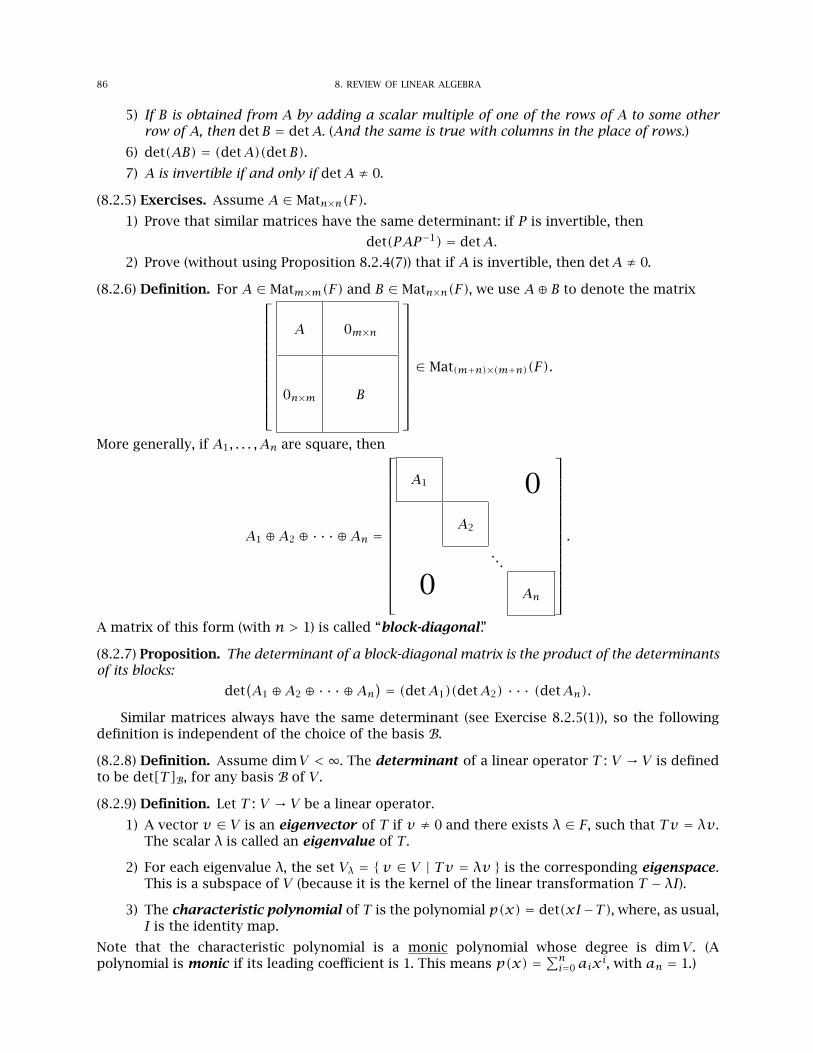
86 8. REVIEW OF LINEAR ALGEBRA
5) If B is obtained from A by adding a scalar multiple of one of the rows of A to some otherrow of A, then detB = detA. (And the same is true with columns in the place of rows.)
6) det(AB) = (detA)(detB).7) A is invertible if and only if detA ≠ 0.
(8.2.5) Exercises. Assume A ∈ Matn×n(F).1) Prove that similar matrices have the same determinant: if P is invertible, then
det(PAP−1) = detA.2) Prove (without using Proposition 8.2.4(7)) that if A is invertible, then detA ≠ 0.
(8.2.6) Definition. For A ∈ Matm×m(F) and B ∈ Matn×n(F), we use A⊕ B to denote the matrix
A 0m×n
0n×m B
∈ Mat(m+n)×(m+n)(F).
More generally, if A1, . . . , An are square, then
A1 ⊕A2 ⊕ · · · ⊕An =
A1 0A2
...
0 An
.
A matrix of this form (with n > 1) is called “block-diagonal .”
(8.2.7) Proposition. The determinant of a block-diagonal matrix is the product of the determinantsof its blocks:
det(A1 ⊕A2 ⊕ · · · ⊕An
) = (detA1)(detA2) · · · (detAn).
Similar matrices always have the same determinant (see Exercise 8.2.5(1)), so the followingdefinition is independent of the choice of the basis B.
(8.2.8) Definition. Assume dimV <∞. The determinant of a linear operator T : V → V is definedto be det[T]B, for any basis B of V .
(8.2.9) Definition. Let T : V → V be a linear operator.
1) A vector v ∈ V is an eigenvector of T if v ≠ 0 and there exists λ ∈ F, such that Tv = λv.The scalar λ is called an eigenvalue of T .
2) For each eigenvalue λ, the set Vλ = {v ∈ V | Tv = λv } is the corresponding eigenspace.This is a subspace of V (because it is the kernel of the linear transformation T − λI).
3) The characteristic polynomial of T is the polynomial p(x) = det(xI−T), where, as usual,I is the identity map.
Note that the characteristic polynomial is a monic polynomial whose degree is dimV . (Apolynomial is monic if its leading coefficient is 1. This means p(x) =∑ni=0 aixi, with an = 1.)
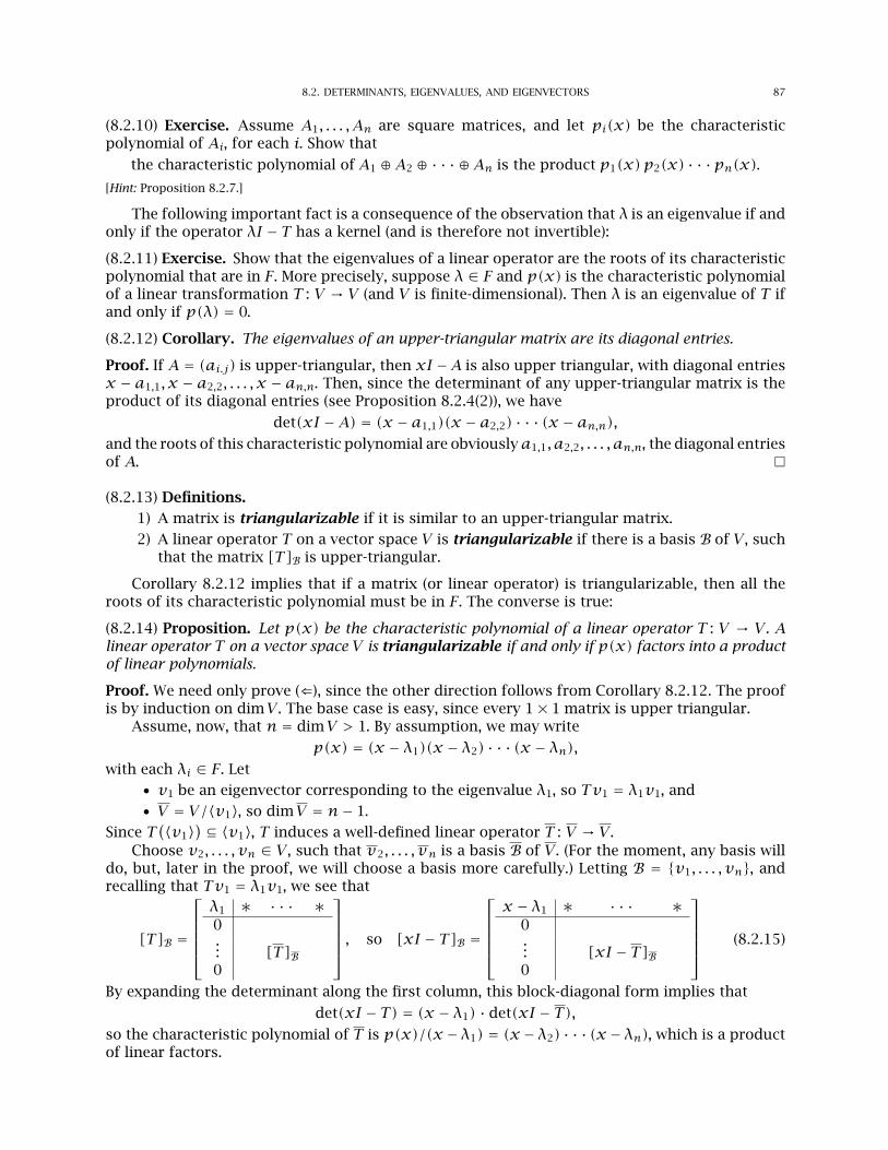
8.2. DETERMINANTS, EIGENVALUES, AND EIGENVECTORS 87
(8.2.10) Exercise. Assume A1, . . . , An are square matrices, and let pi(x) be the characteristicpolynomial of Ai, for each i. Show that
the characteristic polynomial of A1 ⊕A2 ⊕ · · · ⊕An is the product p1(x)p2(x) · · ·pn(x).[Hint: Proposition 8.2.7.]
The following important fact is a consequence of the observation that λ is an eigenvalue if andonly if the operator λI − T has a kernel (and is therefore not invertible):
(8.2.11) Exercise. Show that the eigenvalues of a linear operator are the roots of its characteristicpolynomial that are in F. More precisely, suppose λ ∈ F and p(x) is the characteristic polynomialof a linear transformation T : V → V (and V is finite-dimensional). Then λ is an eigenvalue of T ifand only if p(λ) = 0.
(8.2.12) Corollary. The eigenvalues of an upper-triangular matrix are its diagonal entries.
Proof. If A = (ai.j) is upper-triangular, then xI −A is also upper triangular, with diagonal entriesx − a1,1, x − a2,2, . . . , x − an,n. Then, since the determinant of any upper-triangular matrix is theproduct of its diagonal entries (see Proposition 8.2.4(2)), we have
det(xI −A) = (x − a1,1)(x − a2,2) · · · (x − an,n),and the roots of this characteristic polynomial are obviouslya1,1, a2,2, . . . , an,n, the diagonal entriesof A. □
(8.2.13) Definitions.1) A matrix is triangularizable if it is similar to an upper-triangular matrix.2) A linear operator T on a vector space V is triangularizable if there is a basis B of V , such
that the matrix [T]B is upper-triangular.
Corollary 8.2.12 implies that if a matrix (or linear operator) is triangularizable, then all theroots of its characteristic polynomial must be in F. The converse is true:
(8.2.14) Proposition. Let p(x) be the characteristic polynomial of a linear operator T : V → V . Alinear operator T on a vector space V is triangularizable if and only if p(x) factors into a productof linear polynomials.
Proof. We need only prove (⇐), since the other direction follows from Corollary 8.2.12. The proofis by induction on dimV . The base case is easy, since every 1× 1 matrix is upper triangular.
Assume, now, that n = dimV > 1. By assumption, we may write
p(x) = (x − λ1)(x − λ2) · · · (x − λn),with each λi ∈ F. Let
• v1 be an eigenvector corresponding to the eigenvalue λ1, so Tv1 = λ1v1, and• V = V/⟨v1⟩, so dimV = n− 1.
Since T(⟨v1⟩
) ⊆ ⟨v1⟩, T induces a well-defined linear operator T : V → V .Choose v2, . . . , vn ∈ V , such that v2, . . . , vn is a basis B of V . (For the moment, any basis will
do, but, later in the proof, we will choose a basis more carefully.) Letting B = {v1, . . . , vn}, andrecalling that Tv1 = λ1v1, we see that
[T]B =
λ1 ∗ · · · ∗0... [T]B0
, so [xI − T]B =
x − λ1 ∗ · · · ∗
0... [xI − T]B0
(8.2.15)
By expanding the determinant along the first column, this block-diagonal form implies that
det(xI − T) = (x − λ1) · det(xI − T),so the characteristic polynomial of T is p(x)/(x−λ1) = (x−λ2) · · · (x−λn), which is a productof linear factors.
88 8. REVIEW OF LINEAR ALGEBRA
Hence, by induction on dimV , we may assume that the basis B has been chosen so that [T]Bis upper triangular. Then (8.2.15) shows that [T]B is upper triangular. □
We can combine Proposition 8.2.14 with the following important fact (which means that C is“algebraically closed”):
(8.2.16) Theorem (Fundamental Theorem of Algebra). Every nonconstant polynomial in C[x] hasa root in C.
Idea of proof. We describe one of the many different proofs of this theorem. Others can be foundin textbooks on Complex Analysis or Field Theory, or on wikipedia:
https://en.wikipedia.org/wiki/Fundamental_theorem_of_algebra#ProofsSuppose f(x) ∈ C[x], and f(x) has no roots. Assume, for simplicity, that f(x) is monic, and
let n = deg f(x). For r ≥ 0 and t ∈ [0,2π], let pr (t) = f(reit). For each fixed r , the function pris a closed path in C∖ {0}, and therefore has a winding number w(pr ), which is the net numberof times that pr winds around the origin (counter-clockwise).
The pathp0 is constant, sow(p0) = 0. Sincew(pr ) is always an integer, but is also a continuousfunction of r , this implies that w(pr ) = 0 for all r . However, when r is large, the leading term xnof f(x) is much larger than all others, so it is clear that w(pr ) = n in this case. We conclude thatn = 0, so f(x) is constant. □
(8.2.17) Corollary. Every linear operator on any vector space over C is triangularizable.
Proof. The Fundamental Theorem of Algebra (8.2.16) implies that every nonconstant, irreduciblepolynomial inC[x] is linear, so every nonconstant polynomial inC[x] is a product of linear factors.In particular, If T is a linear operator on a vector space V over C, then the characteristic polynomialof T is a product of linear factors. So Proposition 8.2.14 tells us that T is triangularizable. □
(8.2.18) Example. Let A = [0 −11 0
], so the characteristic polynomial of A is x2 + 1. Since the
polynomial x2 + 1 has no real roots, we see that A is not triangularizable over R. That is, theredoes not exist an invertible matrix P ∈ Mat2×2(R), such that PAP−1 is upper-triangular. In otherwords, if T : R2 → R2 is defined by Tv = Av, then there is no basis B of R2, such [T]B is uppertriangular.
On the other hand, we know from Corollary 8.2.17 thatAmust be similar to an upper-triangularmatrix over C. Indeed, for P =
[1 ii 1
], we have P−1AP =
[i 00 −i
], which is diagonal, not just upper
triangular.
(8.2.19) Exercise. Show that eigenvectors corresponding to different eigenvalues are linearlyindependent.
More precisely, assume1) T : V → V is a linear operator,2) v1, . . . , vk are eigenvectors of T ,3) λi is the eigenvector corresponding to vi (i.e., Tvi = λivi), and4) λi ≠ λj for i ≠ j.
Show that v1, . . . , vk are linearly independent.[Hint: Consider a linear combination that is 0, and has the minimum possible number of nonzero coefficients.]
§8.3. Diagonalizability
Diagonal matrices are easy to work with, but, unfortunately, not every matrix is similar to adiagonal matrix (even when its characteristic polynomial is a product of linear factors):
(8.3.1) Exercise. Show that the matrix[
0 10 0
]is not similar to any diagonal matrix, even though its
characteristic polynomial x2 is a product of linear factors.
8.3. DIAGONALIZABILITY 89
[Hint: If D is a diagonal matrix, with d1, . . . , dn along the main diagonal, then D2 has d21, . . . , d2
n along the main diagonal.Hence, if D ≠ 0, then D2 ≠ 0.]
(8.3.2) Exercise. For a linear operator T : V → V (with dimV < ∞), show that the following areequivalent:
1) T is diagonalizable (that is, there is a basis B of V , such that [T]B is a diagonal matrix).
2) There is a basis of V that consists entirely of eigenvectors of T .
3) V is spanned by the eigenvectors of T .
(8.3.3) Exercise. Suppose T : V → V is a linear operator, with dimV = n < ∞. Show that if T hasn distinct eigenvalues, then it is diagonalizable.
(8.3.4) Definition. For any polynomial p(x) =∑ri=0 aixi ∈ F[x] and A ∈ Matn×n(F), we define
p(A) =r∑i=0
aiAi ∈ Matn×n(F).
For any fixed A, the map p(x), p(A) is a ring homomorphism.
(8.3.5) Proposition. For any A ∈ Matn×n(F), there is a unique monic polynomial m(x) ∈ F[x],such that, for all p(x) ∈ F[x], we have
p(A) = 0 ⇐⇒ m(x) | p(x).We call m(x) the minimal polynomial of A.
Proof. Let I = {p(x) ∈ F[x] | p(A) = 0 }. It is easy to verify that I is an ideal in the ring F[x]. (Infact, it is the kernel of the homomorphism p(x), p(A).) Also, since Matn×n(F) isn2-dimensional,the powers I,A,A2, A3, . . . , An2
cannot be linearly independent, so there exist a0, . . . , an2 ∈ F, notall 0, such that
∑n2
i=0 aiAi = 0. In other words, if we let p0(x) =∑n2
i=0 aixi, then p0(x) ∈ I, so theideal I is nonzero. Since F[x] is a PID (in fact, it is Euclidean), the ideal must be generated by somenonzero m(x) ∈ F[x]. This means that p(x) ∈ I ⇐⇒ m(x) | p(x).
The generator of I is unique up to multiplication by a scalar (that is, by a unit in the ring F[x]),so there is a unique choice of m(x) that is monic. □
(8.3.6) Remark. The proof shows that degm(x) ≤ n2. In fact, the famous Cayley-HamiltonTheorem (10.1.13) will show that degm(x) ≤ n.
(8.3.7) Exercise. Assume A1, . . . , An are square matrices, and letmi(x) be the minimal polynomialof Ai, for each i. Show that
the minimal polynomial of A1 ⊕A2 ⊕ · · · ⊕An is lcm(m1(x),m2(x), . . . ,mn(x)
).
[Hint: p(A1 ⊕ · · · ⊕An
) = p(A1)⊕ · · · ⊕ p(An) for any p(x) ∈ F[x].]
(8.3.8) Proposition. Let A ∈ Matn×n(F). Then A is diagonalizable (via some invertible matrixP ∈ Matn×n(F)) if and only if the minimal polynomial of A is a product of linear factors in F[x]and has no repeated roots.
Proof. Let m(x) be the minimal polynomial of A.(⇒) Suppose A = diag(a1, . . . , an) is a diagonal matrix with a1, . . . , an on the main diagonal.
Let
• λ1, . . . , λk be its distinct eigenvalues (so {a1, . . . , an} = {λ1, . . . , λk}), and
• p(x) =∏kj=1(x − λj), so p(ai) = 0 for all i.
Then, since A is diagonal, we have
p(A) = p(diag(a1, . . . , an)) = diag
(p(a1), p(a2), . . . , p(an)
) = (0,0, . . . ,0) = 0.Therefore m(x) | p(x). From its definition, it is obvious that that p(x) is a product of linearfactors in F[x], and has no repeated roots. The same must be true of the divisor m(x).
90 8. REVIEW OF LINEAR ALGEBRA
(⇐) By assumption, we may writem(x) =∏ki=1(x−λi), where λ1, . . . , λk are distinct. For each i,
let
pi(x) =∏j≠i
(x − λi) = m(x)x − λi.
Since gcd(p1(x),p2(x), . . . , pk(x)
) = 1, and F[x] is a PID, there exist polynomials ui(x) ∈ F[x],such that
u1(x)p1(x)+u2(x)p2(x)+ · · ·uk(x)pk(x) = 1.Let v ∈ Fn be arbitrary. For 1 ≤ i ≤ k, let vi = ui(A)pi(A)v. Then
(A− λi)vi = ui(A)((A− λi)pi(A)
)v = ui(A)m(A)v = ui(A) · 0 · v = 0,
so vi is an eigenvector of A (with eigenvalue λi).Furthermore, we have
v1 + · · ·vk =k∑i=1
ui(A)pi(A)v = k∑i=1
ui(A)pi(A)
v = (I)v = v.Since v is arbitrary, and v1, v2, . . . , vk are eigenvectors, this implies that the eigenvectors of Aspan V . So Exercise 8.3.2 implies that A is similar to a diagonal matrix. □
(8.3.9) Exercise. A square matrix A is said to be nilpotent if there is some k ∈ N, such that Ak = 0.For each n, show that 0 is the only n×n nilpotent matrix that is diagonalizable.[Hint: This is a generalization of Exercise 8.3.1.]
(8.3.10) Remark. Similar matrices have the same minimal polynomial (why?). Therefore, anylinear transformation T : V → V has a well-defined minimal polynomial (if dimV < ∞), andProposition 8.3.8 applies to it.
(8.3.11) Exercise. Assume T is a linear operator on a finite-dimensional vector space V .1) Show that if T 2 = T , then T is diagonalizable.2) Assume W is a subspace of V that is T -invariant . (This means T(W) ⊆ W , so the
restriction T |W is a linear operator on W .) Show that if T is diagonalizable, then T |W isalso diagonalizable.
Chapter 9
Bilinear forms and Hermitian forms
(9.0.1) Notation. Assume F is a field. (Usually, it will be R or C.)
§9.1. Real symmetric matrices are diagonalizable (optional)
(9.1.1) Definitions.1) Recall that the transpose of an m × n matrix A = (ai,j) is the n ×m matrix AT = (aj,i)
whose columns are the rows of A. For example,[1 2 34 5 6
]T
=
1 42 53 6
and
123
T
=[1 2 3
].
2) A matrix A = (ai,j) is symmetric if it is equal to its transpose: AT = A. (This means thatai,j = aj,i for all i, j, so A is symmetric across the main diagonal.) Every symmetric matrixmust have the same number of rows as columns: it is a square matrix.
(9.1.2) Examples.1) Every diagonal matrix is symmetric. (In particular, every 1× 1 matrix is symmetric.)
2) Symmetric matrices that are 2×2 or 3×3 are of the following forms:
[a bb c
],
a b cb d ec e f
.
3) An upper-triangular matrix cannot be symmetric unless it is also lower-triangular, and istherefore a diagonal matrix.
(9.1.3) Exercises.1) Show that transpose is a linear operator on Matm×n(F): (sA+ tB)T = sAT+ tBT for s, t ∈ F
and A,B ∈ Matm×n(F).2) Show that the set of n×n symmetric matrices is a vector subspace of Matn×n(F).3) Show that the transpose of a product is the product of the transposes in the reverse order:
if A ∈ Matm×n(F) and B ∈ Matn×p(F), then (AB)T = BTAT.4) Show that the set of n× n symmetric matrices is closed under powers: if A is symmetric
and k ∈ N, then Ak is symmetric.5) Show that the set of n×n symmetric matrices is not closed under multiplication (if n ≥ 2).6) Show (AT)T = A for all A ∈ Matm×p(F).7) Let A ∈ Matn×n(R). Show that if there is an orthogonal matrix P ∈ Matn×n(R), such thatPAP−1 is a diagonal matrix, then A is symmetric. (Recall that P is orthogonal if PT = P−1.)
(9.1.4) Remark. The converse of Exercise 9.1.3(7) is true (see Remark 9.1.13).
91
92 9. BILINEAR FORMS AND HERMITIAN FORMS
Although some matrices are not diagonalizable (see, for example, Exercise 8.3.1), we will seethat every symmetric matrix with real entries is diagonalizable:
(9.1.5) Theorem. Let A ∈ Matn×n(R). If A is symmetric, then A is diagonalizable.
More precisely, A is diagonalizable over R: there is an invertible matrix P ∈ Matn×n(R), suchthat PAP−1 is a diagonal matrix. The remainder of this section provides a proof of this importanttheorem, by using the following relation between transposes and the dot product:
(9.1.6) Exercise. For v,w ∈ Rn and A ∈ Matn×n(R), show that
v ·Aw = (ATv) ·w,where the dot product on Rn is defined by
(v1, v2, . . . , vn) · (w1,w2, . . . ,wn) = v1w1 + v2w2 + · · · + vnwn.[Hint: Recalling that we identify (v1, v2, . . . , vn)with the corresponding column vector (see Notation 8.1.5), and identifyingMat1×1(R)with R in the obvious way, the dot product may be written in terms of matrix multiplication as: v ·w = vTw.]
This has the following consequences:
(9.1.7) Exercise. Let A be a symmetric matrix in Matn×n(R).
1) For v ∈ Rn, such that A2v = 0, show Av = 0.[Hint: If A2v = 0, then v ·A2v = 0.]
2) Show that if A is nilpotent, then A = 0.
3) Show that the minimal polynomial of A has no repeated real roots: ifm(x) is the minimalpolynomial of A, and c ∈ R, then m(x) is not divisible by (x − c)2.[Hint: A− cI is symmetric. (Why? )]
To show that a real symmetric matrix A is diagonalizable, we wish to show that its minimalpolynomial is a product of linear factors in R[x] and has no repeated roots (see Proposition 8.3.8).Exercise 9.1.7(3) deals with the question of repeated roots, but we still need to show that theminimal polynomial is a product of linear factors. For this, we extend the dot product on Rn to acertain product on Cn:
(9.1.8) Definition. The (standard) Hermitian form on Cn is the function C×C→ C that is definedby ⟨
(z1, z2, . . . , zn)∣∣(w1,w2, . . . ,wn)
⟩ = z1w1 + z2w2 + · · · + znwn.(Recall that the conjugate of a complex number z = x + iy is the complex number z = x − iy.)This is like the dot product, except that the second factor in each summand has been conjugated.
The following crucial property is a good reason for including complex conjugation in thisdefinition:
(9.1.9) Exercise. For v ∈ Cn, show that if ⟨v | v⟩ = 0, then v = 0.
Corresponding to Exercise 9.1.6, we have the following observation:
(9.1.10) Exercise. Suppose v,w ∈ Cn and A ∈ Matn×n(C). Show that ⟨v | Aw⟩ = ⟨A∗v | w⟩,where A∗ is the adjoint (or conjugate-transpose) of A = (ai,j), defined by
A∗ = AT = A T = (aj,i).[Hint: Note that ⟨v | w⟩ = w∗ v.]
(9.1.11) Lemma. Every eigenvalue of a real symmetric matrix is real.
9.2. BILINEAR FORMS 93
Proof. Assume A ∈ Matn×n(R) is symmetric. If Av = λv (with v ≠ 0 and λ ∈ C), then
⟨(A− λI)v | (A− λI)v⟩ = ⟨(A− λI)∗ (A− λI)v | v⟩ (Exercise 9.1.10)
= ⟨(A∗ − λI) (A− λI)v | v⟩ ((sA+ tB)∗ = s A∗ + t B∗ for s, t ∈ C)
= ⟨(A− λI) (A− λI)v | v⟩(
A is symmetric, so AT = A,and A is a real matrix, so A = A
)
= ⟨(A− λI)(A− λI)v | v⟩
A commutes with itself, andthe scalar matrices λI and λI
commute with everything
= ⟨(A− λI)0 | v⟩ (Av = λv)
= ⟨0 | v⟩= 0,
so (A−λI)v = 0 (by Exercise 9.1.9). This means Av = λv. Since Av is also equal to λv (and v ≠ 0),this implies λ = λ, so λ ∈ R. □
Proof of Theorem 9.1.5. Let m(x) be the minimal polynomial of A. From Lemma 9.1.11 and theFundamental Theorem of Algebra (8.2.16), we know that m(x) is a product of linear factors inR[x]. Then all roots ofm(x) are real, so Exercise 9.1.7(3) implies thatm(x)has no repeated roots.We conclude from Proposition 8.3.8 that A is diagonalizable. □
(9.1.12) Exercises.1) Show that the restriction to real matrices in Theorem 9.1.5 cannot be eliminated. More
precisely, show that the symmetric matrix[
1 ii −1
]is not diagonalizable (over C).
[Hint: What is the square of this matrix?]
2) Show that the eigenspaces of a real symmetric matrix are orthogonal to each other: ifAv = λv and Aw = µw, with λ ≠ µ, then v ·w = 0.[Hint: Consider v · Aw. You may use (without proof) the fact that the dot product is “bilinear” in the sense ofDefinition 9.2.1 below (see Example 9.2.2).]
(9.1.13) Remark. If A is a real symmetric n × n matrix, then, by combining Theorem 9.1.5 withExercise 9.1.12(2) and Gram-Schmidt Orthogonalization (cf. Remark 9.4.14), one can show that Rn
has an basis of eigenvectors that is orthonormal. This implies the converse of Exercise 9.1.3(7).
§9.2. Bilinear forms
In this section, we discuss a generalization of the dot product that applies to all vector spaces,not just Rn.
(9.2.1) Definition. A bilinear form on the vector space V is a function B : V × V → F that is linearin each variable, i.e.:
B(a1v1 + a2v2,w) = a1 B(v1,w)+ a2 B(v2,w)
and
B(v, b1w1 + b2w2) = b1 B(v,w1)+ b2 B(v,w2)
(9.2.2) Example. If we define B(x,y) = x · y, then B is a bilinear form on Rn. Note that if weidentify x and y with column vectors [x] and [y] in the natural way, then
B(x,y) = x1y1 + x2y2 + · · · + xnyn = [x1, x2, . . . , xn]
y1
y2...yn
= [x]T [y].
94 9. BILINEAR FORMS AND HERMITIAN FORMS
(9.2.3) Exercise. Let B be a basis of the n-dimensional vector space V .1) If we define B(x,y) = [x]TB [y]B, then B is a bilinear form on V .
2) More generally, for any M ∈ Matn×n(F), the formula BM(x,y) = [x]TBM [y]B defines abilinear form on V . (The previous example is the special case where M = I.)
3) Conversely, every bilinear form on V is equal to BM, for a unique M ∈ Matn×n(F).[Hint: For BM to agree with B on the basis vectors v1, . . . , vn, the matrix M must be
[B(vi, vj)
]. Then, since {vi}
spans V, bilinearity implies BM = B.]
4) Let B be a bilinear form on V . We say that B is nondegenerate if for every nonzero v ∈ V ,there exists w ∈ V , such that B(v,w) ≠ 0. Show that BM is nondegenerate if and only ifthe matrix M is invertible.
5) Show thatv andw can be interchanged in the definition of “nondegenerate.” More precisely,for a bilinear form B on V , show that B is nondegenerate if and only if, for every nonzerow ∈ V , there exists v ∈ V , such that B(v,w) ≠ 0.
(9.2.4) Warning. Exercise 9.2.3(5) is not true if V is allowed to be infinite-dimensional. (IfdimV = ∞, then the definition of nondegenerate should be revised to require both conditions.)
(9.2.5) Exercises. Assume U, V , W , Y , and Z are vector spaces.1) Suppose f : V × W → Y is bilinear and T : Y → Z is linear. Show that the compositionT ◦ f : V ×W → Z is bilinear.
2) Suppose that f : V ×W → U is bilinear and that T1 : Y → V and T2 : Z → W are linear. Showthat the composition f ◦ (T1 × T2) : (Y × Z)→ U is bilinear, where(
f ◦ (T1 × T2))(y, z) = f (T1(y), T2(z)
)for y ∈ Y and z ∈ Z.
3) Suppose• f and g are bilinear functions from V ×W to Z, and• {vi} and {wj} are bases of V and W , respectively,
such that f(vi,wj) = g(vi,wj) for all i and j. Show f = g.
§9.3. Dual space V∗
Suppose dimV = n and dimW =m. Then, by choosing bases of V and W , it is easy to see that thevector space Hom(V ,W) of all linear transformations from V to W is isomorphic to Matm×n(F),so it has dimension mn. The case where m = 1 is particularly important:
(9.3.1) Definition.1) A linear function f : V → F is called a linear functional on V .2) Let V∗ = { linear functionals on V }. It is a vector space under the following operations (forf , g ∈ V∗ and a ∈ F):• (f + g)(v) = f(v)+ g(v) for v ∈ V .• (af)(v) = af(v) for v ∈ V .
This is called the dual space of V .
(9.3.2) Exercise.1) Suppose v ∈ V and f ∈ V∗. Show that if f(v) ≠ 0, then V = Fv ⊕ kerf .2) Let f ,g ∈ V∗. Show kerf = kerg iff there is a nonzero scalar λ, such that f = λg.3) Show (V1 ⊕ V2)∗ is naturally isomorphic to V∗1 ⊕ V∗2 .
[Hint: Define φ: V∗1 ⊕ V∗2 → (V1 ⊕ V2)∗ by φ(f1, f2)(v1, v2) = f1(v1) + f2(v2) and ψ : (V1 ⊕ V2)∗ → V∗1 ⊕ V∗2by ψ(µ) = (
ψ1(µ),ψ2(µ)), where ψ1(µ)(v1) = µ(v1,0) and ψ2(µ)(v2) = µ(0, v2). Show ψ = φ−1. Your proof
should not require the choice of a basis.]
If dimV < ∞, then the above discussion shows that dimV∗ = dimV , so V∗ ≊ V . Here is theusual proof of this fact:
(9.3.3) Proposition. If V is finite-dimensional, then V ≊ V∗.
9.3. DUAL SPACE V∗ 95
Proof. Fix a basis {v1, . . . , vn}of V . Then, for each i, define vi ∈ V∗ by requiring that vi(vi) = 1, butvi(vj) = 0 for all j ≠ i (and extending to make it linear). It is not difficult to see that {v1, . . . , vn} isa basis for V∗. (It is called the dual basis corresponding to {v1, . . . , vn}.) Namely, for any f ∈ V∗,∑i f(vi) vi is the unique linear combination that agrees with f on the basis {vi}, and is therefore
equal to f . This means that V∗ has a basis with n elements, so dimV∗ = n = dimV . ThereforeV ≊ V∗. □
Note that the above proof depends on choosing a basis of V . In fact, there is no canonical wayto choose an isomorphism. However, instead of a basis, it suffices to choose only a bilinear form:
(9.3.4) Exercise. Suppose B is a nondegenerate bilinear form on V , and dimV < ∞. Then there isan isomorphism B : V → V∗, defined by
(Bv)(w) = B(v,w) for v,w ∈ V.[Hint: Verify that Bv ∈ V∗, so B is a function from V to V∗. Then it is easy to check that B is linear. Use the nondegeneracyof B to show that ker B = 0. Since dimV = dimV∗ <∞, this implies that B is an isomorphism.]
(9.3.5) Remark. Conversely, if B : V → V∗ is any isomorphism, then a nondegenerate bilinearform B on V can be defined by the formula B(v,w) = (Bv)(w). Hence, choosing a particularisomorphism from V to V∗ is equivalent to choosing a nondegenerate bilinear form on V (whenV is finite-dimensional).
(9.3.6) Warning. If V is infinite-dimensional, then V ≊ V∗, because dimV∗ > dimV . (The reasonis that if B is a basis of V , then V is isomorphic to the direct sum
⊕v∈B F of infinitely many copies
of F, but V∗ is isomorphic to the direct product∏v∈B F, which is much larger.)
(9.3.7) Definition. The dual space of the dual space is called the double-dual of V , and is denotedV∗∗.
If dimV < ∞, then Proposition 9.3.3 implies V∗∗ = (V∗)∗ ≊ V∗ ≊ V , so V∗∗ ≊ V . Althoughthe isomorphisms from V∗∗ to V∗ and V to V∗ both depend on the choice of a basis (or, at least,a bilinear form), the isomorphism from V to V∗∗ does not require any such choice:
(9.3.8) Proposition. If dimV <∞, then V∗∗ is canonically isomorphic to V .
Proof. For v ∈ V , define v ∈ V∗∗ by v(f ) = f(v), for f ∈ V∗. It is straightforward to verify thatthe map v , v is linear. It is also quite easy to see that it is injective: for any basis of V thatcontains the nonzero vector v, we may let v ∈ V∗ be the corresponding element of the dual basis,and then we have v(v) = v(v) = 1, so v ≠ 0. Since dimV = dimV∗∗ < ∞, this implies that themap is an isomorphism. □
(9.3.9) Remark. When V is infinite-dimensional, the above proof shows that the map v , vis injective (because Zorn’s Lemma provides a basis of V). However, it is not surjective (sincedimV < dimV∗∗).
(9.3.10) Definition. For any linear operator T : V → V , there is an associated linear transformationT T : V∗ → V∗ (sometimes called the transpose of T), defined by
(T Tf)(v) = f(Tv) for all v ∈ V and f ∈ V∗.When V is finite-dimensional, any nondegenerate bilinear form provides an identification of V∗
with V , so the map T T : V∗ → V∗ can be thought of as a function from V to V :
(9.3.11) Proposition. Suppose B is a nondegenerate bilinear form on the finite-dimensional vectorspace V , and T : V → V is linear. Then there is a unique linear transformation T∗ : V → V (calledthe adjoint of T with respect to B), such that
B(v, Tw) = B(T∗v,w) for all v,w ∈ V.
96 9. BILINEAR FORMS AND HERMITIAN FORMS
Proof. (existence) Let T T : V∗ → V∗ be the transpose of T . Exercise 9.3.4 provides an isomorphismB : V → V∗, defined by (Bv)(w) = B(v,w), for v,w ∈ V . Let T∗ = B−1 ◦ T T ◦ B : V → V . Then, forany v,w ∈ V , we have
B(T∗v,w) = (BT∗v)(w) (definition of B)
= (B(B−1 ◦ T T ◦ B)v)(w) (definition of T∗)
= (T T(Bv))(w) (cancel the inverse)
= (Bv)(Tw) (definition of T T)
= B(v, Tw) (definition of B). □(uniqueness) Suppose T ′ is another adjoint of T . Then, for all v,w ∈ V , we must have
B(T ′v,w) = B(T∗v,w), so the bilinearity of B implies B(T ′v − T∗v,w) = 0. Since B isnondegenerate, we conclude that T ′v − T∗v = 0, so T ′v = T∗v.
Alternate proof of existence. Assume, for simplicity, that V = Fn, so there is an invertiblematrix M ∈ Matn×n(F), such that B(v,w) = vTMw for all v,w ∈ Fn (cf. Exercise 9.2.3(3)). GivenT ∈ Matn×n(F), let T∗ = (MTM−1)T, so
B(v, Tw) = vTMTw = vTMTM−1Mw = vT (T∗)TMw = (T∗v)TMw = B(T∗v,w),as desired. □
(9.3.12) Exercise. For the (standard) dot product on Rn, show that the adjoint of any matrix A isits ordinary matrix transpose.[Hint: B(v,w) = vTw. Use the fact that the transpose of a product is the product of the transposes in the reverse order.]
(9.3.13) Exercise. Let
• B be a nondegenerate bilinear form on V , with dimV <∞, and
• S and T be linear operators on V .
Show:
1) (S + T)∗ = S∗ + T∗.
2) (aT)∗ = aT∗, for all a ∈ F.
3) (ST)∗ = T∗S∗.
4) If B is symmetric (which means that B(v,w) = B(w,v) for all v,w ∈ V), then T∗∗ = T(where T∗∗ means (T∗)∗).
5) If T is invertible, then T∗ is also invertible, and (T∗)−1 = (T−1)∗.
(9.3.14) Remark. The adjoint T∗ may not exist when V is infinite-dimensional. For example,suppose V has a basis {vi}∞i=1, such that B(vi, vj) = 0 for i ≠ j, but B(v1, v1) ≠ 0. Define T : V → Vby Tvi = vi + v1, and suppose T∗v1 =
∑ni=1αivi. Then
B(Tvn+1, v1) = B(vn+1 + v1, v1) = B(vn+1, v1)+ B(v1, v1) = 0+ B(v1, v1) ≠ 0,but
B(vn+1, T∗v1) = B(vn+1,
∑ni=1αivi
) =∑ni=1αi B(vn+1, vi
) =∑ni=1αi 0 = 0.This contradicts the fact that B(Tvn+1, v1) = B(vn+1, T∗v1), so the adjoint T∗ does not exist.
§9.4. Hermitian forms and diagonalizability
The ordinary dot product on Rn has the nice property that if v ≠ 0, then v · v ≠ 0. In fact, v · vis a positive number (unless v = 0), so it has a square root, which is the length (or “norm”) of v:
∥v∥ =√v2
1 + v22 + · · · + v2
n =√v · v.
Unfortunately, there is no such bilinear form on Cn (unless n = 1):
9.4. HERMITIAN FORMS AND DIAGONALIZABILITY 97
(9.4.1) Exercise. Suppose B is any bilinear form on Cn, and n ≥ 2. Show there exists some nonzerov ∈ Cn, such that B(v,v) = 0.[Hint: If v,w ∈ Cn with B(w,w) ≠ 0, then B(v + tw,v + tw) is a quadratic polynomial in t.]
We can eliminate this problem by replacing bilinear forms with Hermitian forms:
(9.4.2) Definition. Suppose V is a vector space over C.1) A function B : V × V → C is a Hermitian form if it is linear in the first argument and
conjugate-symmetric. For u,v,w ∈ V and s, t ∈ C, this means:• B(su+ tv,w) = sB(u,w)+ tB(v,w), and• B(v,w) = B(w,v), where z denotes the complex conjugate a − bi of the complex
number z = a+ bi .2) A Hermitian form B on V is nondegenerate if for every nonzero v ∈ V , there existsw ∈ V ,
such that B(v,w) ≠ 0.
(9.4.3) Exercise. Show that any Hermitian form is conjugate linear in the second argument. (Thismeans B(w, su+ tv) = sB(w,u)+ tB(w,v).)(9.4.4) Warning. Many authors (including physicists) reverse the variables: they require a Hermitianform to be linear in the second argument (and conjugate-linear in the first).
(9.4.5) Examples.1) We have the standard Hermitian form on Cn (cf. Definition 9.1.8):
B(v,w) = v1w1 + v2w2 + · · · + vnwnfor v = (v1, . . . , vn) and w = (w1, . . . ,wn). Note that B(v,v) > 0 for all nonzero v.
2) A different Hermitian form B′ on Cn can be defined by
B′(v,w) = v1w1 + v2w2 + · · · + vn−1wn−1 − vnwn.Note that B′(v, v) can be negative (because of the minus sign in front of vnwn).
(9.4.6) Remark. The length (or “norm”) of vector v in Cn is often defined to be
∥v∥ =√|v1|2 + |v2|2 + · · · + |vn|2 =
√v1 v1 + v2 v2 + · · · + vn vn =
√B1(v, v),
for the standard Hermitian form B of Example 9.4.5(1).
We have the following analogue of Proposition 9.3.11:
(9.4.7) Exercises. Suppose B is a nondegenerate Hermitian form on V , with dimV < ∞, andT : V → V is linear.
1) Show there is a unique linear transformation T∗ : V → V (called the adjoint of T withrespect to B), such that
B(v, Tw) = B(T∗v,w) for all v,w ∈ V.2) Show T∗∗ = T .
[Hint: Use the fact that B is conjugate-symmetric.]
3) For the standard Hermitian form B on Cn that is defined in Example 9.4.5(1), show that theadjoint of any matrix A is its conjugate-transpose.[Hint: B(v,w) = vTw.]
(9.4.8) Warning. If dimV < ∞, then any nondegenerate bilinear form provides an isomorphismfrom V to V∗. However, a nondegenerate Hermitian form will provide an isomorphism from Vnot to V∗, but to the conjugate V∗ of V∗. (The conjugate of a vector space V has the same vectoraddition, but uses a different scalar multiplication ∗ that is defined by α∗v = αv.) However, thisis not too serious a problem, because every vector space is isomorphic to its conjugate. (It is easyto see that every basis of V is also a basis of V , so dimV = dimV .)
(9.4.9) Definition. Fix a nondegenerate Hermitian form B on V , and suppose T : V → V is a linearoperator.
98 9. BILINEAR FORMS AND HERMITIAN FORMS
• We say that T is self-adjoint if T∗ = T .
• We say that T is unitary if T∗ = T−1.
• We say that T is normal if T commutes with its adjoint (i.e., T∗T = TT∗).
Note that if T is either self-adjoint or unitary, then it is normal.
(9.4.10) Exercise. Show that T is unitary if and only if B(Tv, Tw) = B(v,w) for all v,w ∈ V .
(9.4.11) Definition. Suppose B is a Hermitian form on V .
1) The orthogonal complement of a subspace W of V is
W⊥ = {v ∈ V | B(v,w) = 0 for allw ∈ W }.This is a subspace of V . (Why? )
2) B is said to be positive-definite if B(v,v) > 0 for all nonzero v ∈ V .
(9.4.12) Exercise. Assume that B is a positive-definite Hermitian form on V , that W is a subspaceof V , and that T : V → V is a linear operator.
1) Show B is nondegenerate.
2) Show V = W ⊕W⊥ if V is finite-dimensional.
3) Assume W is T-invariant.(a) Show that if T is self-adjoint, then W⊥ is T-invariant.
[Hint: It is easy to see that W⊥ is T∗-invariant.]
(b) Show that if T is unitary and dimV <∞, then W⊥ is T-invariant.More generally, if T is normal (and dimV < ∞), then W⊥ is T-invariant, but we will notprove this until Exercise 9.4.19 below, since it is more difficult.
(9.4.13) Definition. A basis {v1, . . . , vn} is orthonormal (with respect to the Hermitian form B) ifB(vi, vi) = 1 for all i, but B(vi, vj) = 0 whenever i ≠ j.
(9.4.14) Remark. The Gram-Schmidt Orthogonalization process is an inductive procedure formodifying any set of vectors in Rn to obtain an orthonormal basis of the span of those vectors. Itimplies that every real vector space has an orthonormal basis. The same idea can be used to showthat if B is any Hermitian form on any complex vector space V , then V has an orthonormal basis(with respect to B).
(9.4.15) Theorem (Spectral Theorem for self-adjoint operators). If dimV < ∞, then every self-adjoint linear operator on V is diagonalizable.
More precisely, assume:
• B is a positive-definite Hermitian form on a finite-dimensional vector space V over C, and
• T : V → V is a self-adjoint linear operator.
Then T is diagonalizable.In fact, V has an orthonormal basis consisting of eigenvectors of V .
Proof. Since C is algebraically closed, we know that the characteristic polynomial of T has a root,so T has an eigenvector w. (Multiplying by a scalar, we may assume B(w,w) = 1.) Let W = Cw.Then W is clearly T-invariant, so Exercise 9.4.12(3a) tells us that W⊥ is also T-invariant.
Let T⊥ and B⊥ be the restrictions of T and B to W⊥. Then B⊥ is a positive-definite Hermitianform and T⊥ is a self-adjoint linear transformation. (Why?) Therefore, by induction on dimV , wemay assume there is an (orthonormal) basis v1, . . . , vn−1 ofW⊥ that consists of eigenvectors of T⊥.Then {v1, . . . , vn−1,w} is an (orthonormal) basis of V that consists of eigenvectors of T . □
(9.4.16) Exercise. Let U ∈ Matn×n(C), and let B be the standard Hermitian form on Cn (defined inExample 9.4.5(1)). Show that the following are equivalent:
1) The map v , Uv is a unitary operator (with respect to the Hermitian form B).
2) U−1 is the conjugate-transpose of U.
9.5. TENSOR PRODUCTS OF VECTOR SPACES (advanced) 99
3) For every orthonormal basis {v1, . . . , vn} of Cn (with respect to the Hermitian form B), theset {Uv1, . . . , Uvn} is also an orthonormal basis.
If these conditions hold, the matrix U is said to be unitary .
(9.4.17) Corollary. Suppose A is a self-adjoint matrix in Matn×n(C) (which means that A is equal toits conjugate-transpose). Then there is a unitary matrix U, such that UAU−1 is diagonal.
All normal operators, not only the self-adjoint ones, are diagonalizable by an orthonormalbasis. However, the proof takes a little more work, because it is not so obvious in this case thatthe orthogonal complement of an invariant subspace is invariant. The following exercise outlinesthe proof.
(9.4.18) Exercise. Assume:
• B is a positive-definite Hermitian form on a finite-dimensional vector space V ,
• T : V → V is a normal linear operator, and
• λ,µ ∈ C.
Show:
1) kerT = kerT∗.[Hint: v ∈ kerT ⇒ 0 = B(Tv, Tv) = B(T∗Tv,v) = B(TT∗v,v) = B(T∗v,T∗v).]
2) If Tv = λv, then T∗v = λv.[Hint: Apply (1) to T − λI.]
3) If Tv = λv and Tw = µw, with λ ≠ µ, then B(v,w) = 0.[Hint: λB(v,w) = B(Tv,w) = B(v, T∗w) = B(v, µw) = µB(v,w).]
4) If T kv = 0, for some k ∈ N, then Tv = 0.[Hint: 0 = B(T 2v,T 2v) = B(T∗Tv, T∗Tv)⇒ T∗Tv = 0 ⇒ 0 = B(T∗Tv,v) = B(Tv, Tv).]
5) T is diagonalizable.[Hint: Applying (4) to T − λI shows that the minimal polynomial of T has no repeated roots.]
6) V has an orthonormal basis consisting of eigenvectors of T .[Hint: Choose an orthonormal basis of each eigenspace of T, and let B be the union of all these vectors. Then(5) implies that B spans V, and (3) implies that all the vectors in B are orthogonal to each other.]
(9.4.19) Exercise. Assume
• B is a positive-definite Hermitian form on a finite-dimensional vector space V ,
• T : V → V is a normal linear operator, and
• W is a T-invariant subspace of V .
Show that W⊥ is T-invariant.[Hint: You may assume Exercise 9.4.18.]
Exercise 9.4.18 implies Theorem 9.1.5:
(9.4.20) Exercise. Let A ∈ Matn×n(R), such that AT = A. (I.e., A is symmetric .) Show that A isdiagonalizable (over R).[Hint: Exercise 9.4.18(2) shows that the eigenvalues of A are real.]
§9.5. Tensor products of vector spaces (advanced)
(9.5.1) Example. Consider F[x] and F[y], the polynomial rings over F with two different variablesx and y. Each of these is a vector space over F, and we can multiply elements of F[x] by elementsof F[y]. For example, taking 2+ 5x ∈ F[x] and 3−y + 4y2 ∈ F[y], we have
(2+ 5x)(3−y + 4y2) = 6+ 15x − 2y − 5xy + 8y2 + 20xy2.Note that the result of such a multiplication is (usually) not in F[x] or F[y], but in the vectorspace F[x,y] of polynomials in two variables.
100 9. BILINEAR FORMS AND HERMITIAN FORMS
The tensor product is an idea that generalizes this, allowing the elements of any vector space Vto be multiplied by the elements of any other vector space W . For v ∈ V and w ∈ W , the resultof multiplying v times w is written v ⊗w, and belongs to a vector space V ⊗W , called the tensorproduct of V and W .
For example, F[x]⊗ F[y] = F[x,y]. Note that• {xi} is a basis of F[x],• {yj} is a basis of F[y], and• {xiyj} is a basis of F[x,y].
Therefore, if V = F[x] and W = F[y], then a basis of V ⊗W can be obtained by multiplying everyelement of a basis of V by every element of a basis of W . This is true in general:
(9.5.2) Definition. Suppose {vi} and {wj} are bases of V and W , respectively. Then the tensorproduct V ⊗W is the vector space whose basis is the set of all symbols vi ⊗wj. Furthermore, for
v =∑αivi ∈ V and w =
∑βjwj ∈ W,
we definev ⊗w =
∑αiβj (vi ⊗wj).
(9.5.3) Observation. Since {vi ⊗wj} is a basis of V ⊗W , it is obvious that
dim(V ⊗W) = (dimV) · (dimW).
(9.5.4) Warning. Not every element of V ⊗W is of the form v⊗w (such elements are called “pure”tensors or “decomposable” tensors), unless either dimV or dimW is 0 or 1 (see Exercise 9.5.14(2)).Instead, most elements are a sum of elements of this form. For example, most polynomials inF[x,y] (such as 1+ xy) are not of the form f(x)g(y).
The following straightforward exercise shows that this multiplication of vectors is distributive(and that scalars can be pulled out):
(9.5.5) Exercise. Show that the map (v,w) , v ⊗w is bilinear. More precisely, for v,v1, v2 ∈ V ,w,w1,w2 ∈ W , and α ∈ F, we have:
a) (v1 + v2)⊗w = v1 ⊗w + v2 ⊗w,b) v ⊗ (w1 +w2) = v ⊗w1 + v ⊗w2, andc) (αv)⊗w = α(v ⊗w) = v ⊗ (αw).
(9.5.6) Exercise. Show that if v and w are nonzero vectors in V and W , respectively, then theelement v ⊗w of V ⊗W is nonzero.
(9.5.7) Remarks.1) It can be shown that V ⊗ W does not depend on the choice of the bases {vi} and {wi}
(cf. Corollary 9.5.11). In fact, there are alternative definitions of V ⊗W that do not use abasis at all. In particular, some textbooks take the “universal” property in Proposition 9.5.9below as the definition of V ⊗W . Others define V ⊗W to be the vector space spanned bythe symbols v ⊗w, for v ∈ V and w ∈ W , subject only to relations (in 9.5.5(a,b,c)) thatmake the map (v,w), v ⊗w bilinear.
2) Although we have defined the tensor product only for vector spaces, it can actually bedefined for modules over any (commutative) ring. Since most modules do not have a basis,Definition 9.5.2 cannot be used, so one of the other approaches mentioned in (1) is neededfor the generalization.
Warning. In the setting of rings and modules, Exercise 9.5.6 is not usually valid: thereoften exist nonzero m ∈ M and n ∈ N, such that m⊗n = 0 in M ⊗N.
(9.5.8) Exercise. Show that if {v′i} spans V and {w′j} spans W , then {v′i ⊗w′
j} spans V ⊗W .
[Hint: Given v ∈ V and w ∈ W, write v = ∑αiv′i and w = ∑βjw′j. Then use bilinearity to show that v ⊗w is in the span
of {v′i ⊗w′j}.]
9.5. TENSOR PRODUCTS OF VECTOR SPACES (advanced) 101
The following fundamental property is usually much more useful than Definition 9.5.2.More precisely, if you remember this proposition (and other basic facts, such as Exercises 9.5.5and 9.5.8), then you will almost never need (or want) Definition 9.5.2.
(9.5.9) Proposition (Universal property of the tensor product). Assume V , W , and Z are vectorspaces over F. For any bilinear function f : V ×W → Z, there is a unique linear map T : V ⊗W → Z,such that T(v ⊗w) = f(v,w) for all v ∈ V and w ∈ W .
Proof. Since {vi ⊗wj} is a basis, there is a unique linear transformation T : V ⊗W → Z, such thatT(vi⊗wj) = f(vi,wj) for all i and j. (This establishes the uniqueness.) Now, given v =∑αivi ∈ Vand w =∑βjwj ∈ W , combining the bilinearity of ⊗ and f with the linearity of T yields
T(v ⊗w) =∑αiβj T(vi ⊗wj) =
∑αiβj f(vi ⊗wj) = f(v ⊗w),
as desired. □
(9.5.10) Remark. Similar universal properties are common in algebra: saying an object U is“universal” means that every object O with a certain property is a quotient of that object (or,equivalently, that there is a homomorphism from U to O). For example, we have seen that everygroup with an n-element generating set is a quotient of the free group on n generators, so freegroups are universal. Similarly, free modules are universal, because every module is a quotient ofa free module.
Two examples we have already seen are:
1) Suppose G is the free group on a set X. If f is any function from X to a group H, thenthere is a unique homomorphism φ : G → H, such that φ(x) = f(x) for all x ∈ X(see Theorem 4.2.9)
2) Suppose S is a basis for a free module M over R. If f is any function from S to an R-module N, then there is a unique homomorphism φ : M → N, such that φ(s) = f(s) forall s ∈ S (see Exercise 6.4.7(4)).
The following fundamental result is a strengthening of Exercise 9.5.6. It shows that (up toisomorphism) V ⊗W is independent of the choice of basis.
(9.5.11) Corollary. If {v′i} and {w′j} are any bases of V and W , respectively, then {v′i ⊗w′
j} is abasis of V ⊗W .
Proof. From Exercise 9.5.8, it suffices to show that {vi⊗wj} is linearly independent. Let { vi} and{wj} be the linear functionals in V∗ and W∗ that are dual to the bases {vi} and {wj} (as in theproof of Proposition 9.3.3), and fix some i0 and j0. Then there is a bilinear function f : V ×W → Fdefined by f(v,w) = vi0(v) wj0(w). Let T : V ⊗W → F be the corresponding linear map providedby the universality of the tensor product. If
∑αi,j vi ⊗wj = 0, then
0 = T(0) = T(∑
αi,jvi ⊗wj)=∑αi,j vi0(vi) wj0(wj) = αi0,j0 · 1 · 1 = αi0,j0 .
Since i0 and j0 are arbitrary, we conclude that αi,j = 0 for all i and j. So {vi ⊗ wj} is linearlyindependent. □
(9.5.12) Exercise. Show that if {v′i} and {w′j} are linearly independent subsets of V and W ,
respectively, then {v′i ⊗w′j} is a linearly independent subset of V ⊗W .
[Hint: Extend {v′i} and {w′j} to bases and apply Corollary 9.5.11.]
(9.5.13) Example. We can use the universal property to show that F[x]⊗ F[y] ≊ F[x,y].Proof. The function B : F[x]×F[y]→ F[x,y], defined by B
(f(x), g(y)
) = f(x)g(y), is obviouslybilinear, so the universality of the tensor product implies there is a corresponding linear mapT : F[x] ⊗ F[y] → F[x,y]. Since it maps the basis {xi ⊗ yj} of F[x] ⊗ F[y] to the basis {xiyj}of F[x,y], T is an isomorphism. □
102 9. BILINEAR FORMS AND HERMITIAN FORMS
(9.5.14) Exercises.
1) Suppose {wi} is a basis of W . Show that every element of V ⊗W can be written uniquelyin the form
∑vi ⊗wi, where vi ∈ V .
2) Assume {v1, v2} and {w1,w2} are pairs of linearly independent vectors in V and W ,respectively. Show that v1 ⊗w1 + v2 ⊗w2 is not a pure tensor.[Hint: For v =∑i aivi and w =∑j bjwj, use Corollary 9.5.11 to show that v ⊗w ≠ v1 ⊗w1 + v2 ⊗w2.]
3) Is the image of a bilinear function f : V ×W → Z always a subspace of Z?4) Suppose v1, v2 ∈ V and w1,w2 ∈ W , such that v1 ⊗w1 ≠ 0. Show that v1 ⊗w1 = v2 ⊗w2
iff there exists some nonzero α ∈ F, such that v2 = αv1 and w2 = (1/α)w1.5) Suppose V ′ and W ′ are subspaces of V and W , respectively.
(a) Show that V ′⊗W ′ can naturally be identified with a subspace of V⊗W . More precisely,show that if T : V ′ ⊗ W ′ → V ⊗ W is the unique linear transformation such thatT(v ⊗w) = v ⊗w for v ∈ V ′ and w ∈ W ′, then T is an isomorphism onto its image.
(b) Show that if V ′ ⊗W ′ = V ⊗W , then V ′ = V and W ′ = W .6) Show that the tensor product of vector spaces is commutative, distributive, and associative:
(a) V ⊗W is naturally isomorphic to W ⊗ V ,(b) U ⊗ (V ⊕W) is naturally isomorphic to (U ⊗ V)⊕ (U ⊗W), and(c) (U ⊗ V)⊗W is naturally isomorphic to U ⊗ (V ⊗W).
By comparing dimensions, we see that Fm⊗Fn is isomorphic to Fmn, and it is also isomorphicto Matmn(F). Since Matmn(F) can be identified with the vector space HomF(Fm, Fn) of all lineartransformations from Fm to Fn, and Fm ≊ (Fm)∗, this implies that (Fm)∗ ⊗ Fn ≊ HomF
(Fm, Fn
).
We have the following generalization:
(9.5.15) Exercise. Show that if dimW <∞, then V∗ ⊗W is naturally isomorphic to HomF(V ,W).[Hint: There is a linear transformation T : V∗ ⊗ W → HomF (V ,W), such that T(f ⊗ w)(v) = f(v)w. Choose a basis{w1, . . . ,wn}ofW, and let {w1, . . . , wn}be the dual basis. To show T is onto, note that wi◦S ∈ V∗, for any S ∈ HomF (V ,W).To show T is one-to-one, note that any element of V∗ ⊗W can be written in the form
∑fi ⊗wi.]
(9.5.16) Remark. More generally, without any assumption on dimW , it is not difficult to see thatV∗ ⊗W is naturally isomorphic to the subspace Homf.d.
F (V ,W) of HomF(V ,W) consisting of thelinear transformations with finite-dimensional range.
(9.5.17) Exercise. There is a natural linear map τ : V∗ ⊗ V → F, defined by τ(f ⊗ v) = f(v).Show that if V is finite-dimensional, and V∗ ⊗ V is identified with HomF(V , V) in the natural way(see Exercise 9.5.15), then τ(T) is the trace of T , for all T ∈ HomF(V , V).
(Recall that if A = (ai,j) ∈ Matn×n, then the trace of A is the sum of the diagonal entries of A:traceA = a1,1 + · · · + an,n. And the trace of a linear operator T : V → V is defined by choosing abasis of V , and letting T be the trace of the matrix corresponding to T . This exercise provides adifferent definition of the trace of a linear transformation, without any need to choose a basis. )
The following fundamental result shows that the tensor product is completely determined (upto isomorphism) by the universal property in Proposition 9.5.9. Therefore, this universality canbe (and often is!) taken as the definition of the tensor product.
(9.5.18) Corollary. Assume U, V , W , and Z are vector spaces over F, and that ⊠ : V × W → U isbilinear. Also assume that, for any bilinear function f : V ×W → U, there is a unique linear mapT : U → Z, such that T(v ⊠ w) = f(v,w) for all v ∈ V and w ∈ W . Then there is a uniqueisomorphism φ : V ⊗W ≊→ U, such that φ(v ⊗w) = v ⊠w, for all (v,w) ∈ V ×W .
Proof. Since ⊠ is bilinear, the universality of the tensor product implies there is a linear mapφ : V⊗W → U, such thatφ(v⊗w) = v⊠w, for all (v,w) ∈ V×W . Similarly, since (v,w), v⊗wis bilinear, the assumed universality of U implies there is a linear map ψ : U → V ⊗W , such thatψ(v ⊠w) = v ⊗w, for all (v,w) ∈ V ×W . Then, for all (v,w) ∈ V ×W , we have
(ψ ◦φ)(v ⊗w) = ψ(φ(v ⊗w)) = ψ(v ⊠w) = v ⊗w.
9.5. TENSOR PRODUCTS OF VECTOR SPACES (advanced) 103
However, the uniqueness in Proposition 9.5.9 implies that the identity map is the unique linearmap T : V ⊗W → V ⊗W , such that T(v⊗w) = v⊗w. Soψ◦φmust be the identity map on V ⊗W .Similarly, the uniqueness of maps U → Z (with Z = U) implies thatφ◦ψmust be the identity mapon U. Hence, φ is an isomorphism. □
(9.5.19) Exercises.1) There is a natural homomorphism Λ : V∗ ⊗W∗ → (V ⊗W)∗ that satisfies(
Λ(f ⊗ g))(v ⊗w) = f(v)g(w).(a) Show that Λ is one-to-one.(b) Show that Λ is onto if and only if either V or W is finite-dimensional.
2) Generalizing (1), show that if V , W , and Z are vector spaces, then HomF(V ⊗ W,Z) isnaturally isomorphic to HomF
(V,HomF(W,Z)
).
[Hint: Given f ∈ Hom(V ⊗W,Z), any fixed v ∈ V yields a homomorphism from W to Z. Conversely, any elementof Hom
(V,HomF (W,Z)
)yields a bilinear function from V ×W to Z.]
3) Suppose T1 : V1 → W1 and T2 : V2 → W2 are linear transformations.(a) Show there is a unique linear transformation T1 ⊗ T2 : V1 ⊗ V2 → W1 ⊗W2, such that(T1 ⊗ T2)(v1 ⊗ v2) = T1(v1)⊗ T2(v2) for all v1 ∈ V1 and v2 ∈ V2.
(b) Show the image of T1 ⊗ T2 is T1(V1)⊗ T2(V2).(c) Show ker(T1 ⊗ T2) = (kerT1)⊗ V2 + V1 ⊗ (kerT2).(d) Assume V1 = W1 and V2 = W2, so T1 and T2 are linear operators. Show that if T1 and T2
are diagonalizable, then T1 ⊗ T2 is diagonalizable.(e) The map (T1, T2), T1 ⊗ T2 is bilinear, so it yields a linear transformation
Λ : HomF(V1,W1)⊗HomF(V2,W2)→ HomF(V1 ⊗ V2,W1 ⊗W2).Show that if V1, V2, W1, and W2 are finite-dimensional, then Λ is an isomorphism.

Chapter 10
Jordan Canonical Form
(10.0.1) Notation.
• F is a field,
• F[x] is the ring of polynomials over F, and
• Matn×n(F) is the ring of n×nmatrices with entries in F.
For A1, A2 ∈ Matn×n(F), recall that A1 is similar to A2 if there exists an invertible matrixP ∈ Matn×n(F), such that PA1P−1 = A2. (This is an equivalence relation.) Another way of sayingthis is that A1 and A2 represent the same linear transformation from Fn to Fn, but with respectto different bases.
We would like a nice way to find all of the different possible n×nmatrices, up to similarity.This will provide us with an easy way to decide whether two matrices are similar, and will also tellus all of the different linear transformations from Fn to itself, up to a change of basis.
Several solutions to this problem are known, but we will only talk about two of the mostfamous ones: Jordan Canonical Form and Rational Canonical Form.
§10.1. What is Jordan Canonical Form, and what is it good for?
(10.1.1) Assumption. In this section:
All vector spaces are over C.(That is, we assume F = C.)
We make this assumption because it implies that every polynomial in F[x] is a product of linearfactors (so Proposition 8.2.14 tells us that every square matrix is similar to an upper-triangularmatrix, but we will actually be providing a new proof of this fact).
It is important to remember that some matrices cannot be diagonalized (i.e., they are notsimilar to a diagonal matrix), even over C:
(10.1.2) Exercise. Let J =
0 1 0 00 0 1 00 0 0 10 0 0 0
. Show:
1) The minimal polynomial of J is x4.[Hint: Verify that J4 = 0, but J3 ≠ 0.]
2) J is not similar to a diagonal matrix (over any field).[Hint: Proposition 8.3.8 or Exercise 8.3.9.]
105
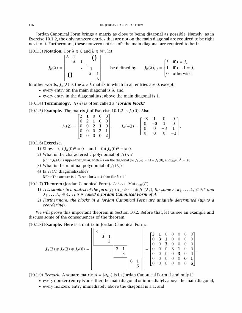
106 10. JORDAN CANONICAL FORM
Jordan Canonical Form brings a matrix as close to being diagonal as possible. Namely, as inExercise 10.1.2, the only nonzero entries that are not on the main diagonal are required to be rightnext to it. Furthermore, these nonzero entries off the main diagonal are required to be 1:
(10.1.3) Notation. For λ ∈ C and k ∈ N+, let
Jk(λ) =
λ 1λ 1 . . .
0. . . 1
λ 10 λ
be defined by Jk(λ)i,j =
λ if i = j,1 if i+ 1 = j,0 otherwise.
In other words, Jk(λ) is the k× kmatrix in which in all entries are 0, except:• every entry on the main diagonal is λ, and• every entry in the diagonal just above the main diagonal is 1.
(10.1.4) Terminology. Jk(λ) is often called a “Jordan block.”
(10.1.5) Example. The matrix J of Exercise 10.1.2 is J4(0). Also:
J5(2) =
2 1 0 0 00 2 1 0 00 0 2 1 00 0 0 2 10 0 0 0 2
, J4(−3) =
−3 1 0 00 −3 1 00 0 −3 10 0 0 −3
.(10.1.6) Exercise.
1) Show (a) Jk(0)k = 0 and (b) Jk(0)k−1 ≠ 0.2) What is the characteristic polynomial of Jk(λ)?
[Hint: Jk(λ) is upper-triangular, with λ’s on the diagonal (or Jk(λ) = λI + Jk(0), and Jk(0)k = 0).]
3) What is the minimal polynomial of Jk(λ)?4) Is Jk(λ) diagonalizable?
[Hint: The answer is different for k = 1 than for k > 1.]
(10.1.7) Theorem (Jordan Canonical Form). Let A ∈ Matn×n(C).1) A is similar to a matrix of the form Jk1(λ1)⊕· · ·⊕ Jkr (λr ), for some r , k1, . . . , kr ∈ N+ andλ1, . . . , λr ∈ C. This is called a Jordan Canonical Form of A.
2) Furthermore, the blocks in a Jordan Canonical Form are uniquely determined (up to areordering).
We will prove this important theorem in Section 10.2. Before that, let us see an example anddiscuss some of the consequences of the theorem.
(10.1.8) Example. Here is a matrix in Jordan Canonical Form:
J3(3)⊕ J2(3)⊕ J2(6) =
3 13 1
3
3 13
6 16
=
3 1 0 0 0 0 00 3 1 0 0 0 00 0 3 0 0 0 00 0 0 3 1 0 00 0 0 0 3 0 00 0 0 0 0 6 10 0 0 0 0 0 6
.
(10.1.9) Remark. A square matrix A = (ai,j) is in Jordan Canonical Form if and only if• every nonzero entry is on either the main diagonal or immediately above the main diagonal,• every nonzero entry immediately above the diagonal is a 1, and
10.1. WHAT IS JORDAN CANONICAL FORM, AND WHAT IS IT GOOD FOR? 107
• whenever a 1 appears above the diagonal, the two diagonal entries adjacent to it (the oneto its left and the one below it) are equal.
More precisely, for 1 ≤ i, j ≤ n, we have:
ai,j ≠ 0 ⇒ j ∈ {i, i+ 1}, ai,i+1 ∈ {0,1}, and ai,i+1 = 1 ⇒ ai,i = ai+1,i+1.
Finding the Jordan Canonical Form of matrices makes it easy to tell whether they are similar:
(10.1.10) Corollary. Let A,A′ ∈ Matn×n(C). Suppose A is similar to J1 ⊕ · · · ⊕ Jr and A′ is similarto J′1 ⊕ · · · ⊕ J′s, where each Ji and J′i is a Jordan block. Then the matrices A and A′ are similar ifand only if r = s and, after a reordering, we have Ji = J′i for every i.
(10.1.11) Observation. It is easy to find the eigenvalues, characteristic polynomial, and minimalpolynomial of any matrix in Jordan Canonical Form.
1) Since the Jordan Canonical Form of any matrix is upper triangular, its eigenvalues arethe numbers that appear on the main diagonal (see Corollary 8.2.12). For example, theeigenvalues of the matrix in Example 10.1.8 are 3 and 6.
2) In general, the characteristic polynomial of a block-diagonal matrix is the product ofthe characteristic polynomials of the blocks (see Exercise 8.2.10). Since the characteristicpolynomial of Jk(λ) is (x − λ)k (see Exercise 10.1.6(2)), we conclude that
the characteristic polynomial ofr⊕i=1
Jki(λi) isr∏i=1
(x − λi)ki.
3) On the other hand, the minimal polynomial of a block-diagonal matrix is the least commonmultiple (not the product!) of the minimal polynomials of the blocks (see Exercise 8.3.7).Therefore, if the set of eigenvalues is {µ1, . . . , µs} where the µi’s are distinct, and we letmj = max{ki | λi = µj } for each j, then, since lcm
((x − µj)k, (x − µj)ℓ
) = (x − µj)max(k,ℓ),
the minimal polynomial ofr⊕i=1
Jki(λi) iss∏j=1
(x − µj)mj.
(10.1.12) Remark. The minimal polynomial is not equal to the characteristic polynomial, unlessthe occurrences of each eigenvalue λ are all in one block. (That is, λi ≠ λj whenever i ≠ j.) Thisis because the exponent of (x − λ) in the characteristic polynomial is the sum of the sizes of theλ-blocks, but the exponent in the minimal polynomial is the maximum of the sizes.
These observations have the following important theoretical consequence:
(10.1.13) Corollary (Cayley-Hamilton Theorem). Every square matrix satisfies its characteristicpolynomial. More precisely, if f(x) is the characteristic polynomial of a matrix A ∈ Matn×n(F),then f(A) = 0.
Proof. Observation 10.1.11 shows that the characteristic polynomial is always a multiple of theminimal polynomial (because the product of any number of polynomials is always a multiple ofthe least common multiple, or, if you prefer to use Remark 10.1.12, it is because the sum of anycollection of natural numbers is always at least as large as the maximum of the numbers). □
(10.1.14) Warning. Students sometimes erroneously believe the Cayley-Hamilton Theorem isobvious, thinking that, since p(x) = det(xI −A), we can simply substitute A for x, to obtain
p(A) = det(AI −A) = det(A−A) = 0.However, this argument is nonsensical. For example, the expression p(A) on the left-hand side isan n × n matrix, but the number 0 on the right-hand side is a scalar (since it is the determinantof a matrix, not the matrix itself), so the two sides certainly cannot be equal (unless n = 1).
With Observation 10.1.11 or Remark 10.1.12 in mind, it is not difficult to find all of the n×nmatrices with a given characteristic polynomial or minimal polynomial (or both), up to similarity.It is much like finding all of the abelian groups of a given finite order, up to isomorphism (as inExercise 7.3.7).
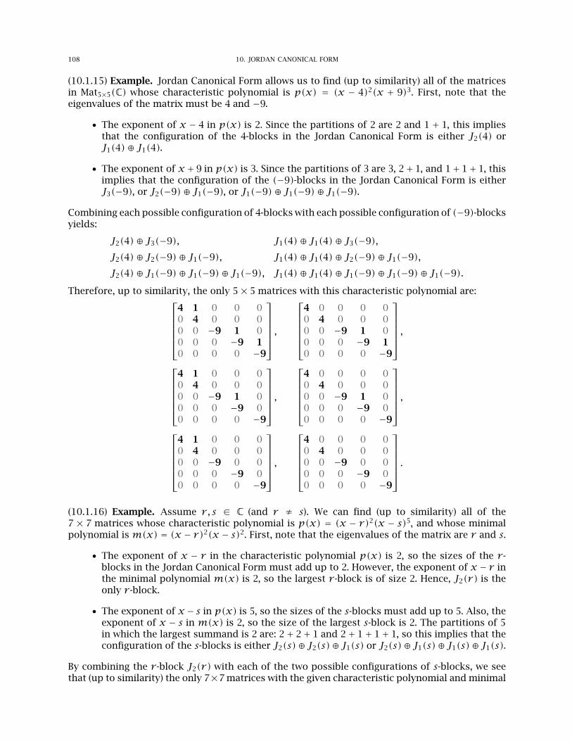
108 10. JORDAN CANONICAL FORM
(10.1.15) Example. Jordan Canonical Form allows us to find (up to similarity) all of the matricesin Mat5×5(C) whose characteristic polynomial is p(x) = (x − 4)2(x + 9)3. First, note that theeigenvalues of the matrix must be 4 and −9.
• The exponent of x − 4 in p(x) is 2. Since the partitions of 2 are 2 and 1 + 1, this impliesthat the configuration of the 4-blocks in the Jordan Canonical Form is either J2(4) orJ1(4)⊕ J1(4).
• The exponent of x+ 9 in p(x) is 3. Since the partitions of 3 are 3, 2+ 1, and 1+ 1+ 1, thisimplies that the configuration of the (−9)-blocks in the Jordan Canonical Form is eitherJ3(−9), or J2(−9)⊕ J1(−9), or J1(−9)⊕ J1(−9)⊕ J1(−9).
Combining each possible configuration of 4-blocks with each possible configuration of (−9)-blocksyields:
J2(4)⊕ J3(−9), J1(4)⊕ J1(4)⊕ J3(−9),
J2(4)⊕ J2(−9)⊕ J1(−9), J1(4)⊕ J1(4)⊕ J2(−9)⊕ J1(−9),
J2(4)⊕ J1(−9)⊕ J1(−9)⊕ J1(−9), J1(4)⊕ J1(4)⊕ J1(−9)⊕ J1(−9)⊕ J1(−9).
Therefore, up to similarity, the only 5× 5 matrices with this characteristic polynomial are:4 1 0 0 00 4 0 0 00 0 −9 1 00 0 0 −9 10 0 0 0 −9
,
4 0 0 0 00 4 0 0 00 0 −9 1 00 0 0 −9 10 0 0 0 −9
,
4 1 0 0 00 4 0 0 00 0 −9 1 00 0 0 −9 00 0 0 0 −9
,
4 0 0 0 00 4 0 0 00 0 −9 1 00 0 0 −9 00 0 0 0 −9
,
4 1 0 0 00 4 0 0 00 0 −9 0 00 0 0 −9 00 0 0 0 −9
,
4 0 0 0 00 4 0 0 00 0 −9 0 00 0 0 −9 00 0 0 0 −9
.
(10.1.16) Example. Assume r , s ∈ C (and r ≠ s). We can find (up to similarity) all of the7 × 7 matrices whose characteristic polynomial is p(x) = (x − r)2(x − s)5, and whose minimalpolynomial is m(x) = (x − r)2(x − s)2. First, note that the eigenvalues of the matrix are r and s.
• The exponent of x − r in the characteristic polynomial p(x) is 2, so the sizes of the r-blocks in the Jordan Canonical Form must add up to 2. However, the exponent of x − r inthe minimal polynomial m(x) is 2, so the largest r-block is of size 2. Hence, J2(r) is theonly r-block.
• The exponent of x− s in p(x) is 5, so the sizes of the s-blocks must add up to 5. Also, theexponent of x − s in m(x) is 2, so the size of the largest s-block is 2. The partitions of 5in which the largest summand is 2 are: 2+ 2+ 1 and 2+ 1+ 1+ 1, so this implies that theconfiguration of the s-blocks is either J2(s)⊕ J2(s)⊕ J1(s) or J2(s)⊕ J1(s)⊕ J1(s)⊕ J1(s).
By combining the r-block J2(r) with each of the two possible configurations of s-blocks, we seethat (up to similarity) the only 7×7 matrices with the given characteristic polynomial and minimal
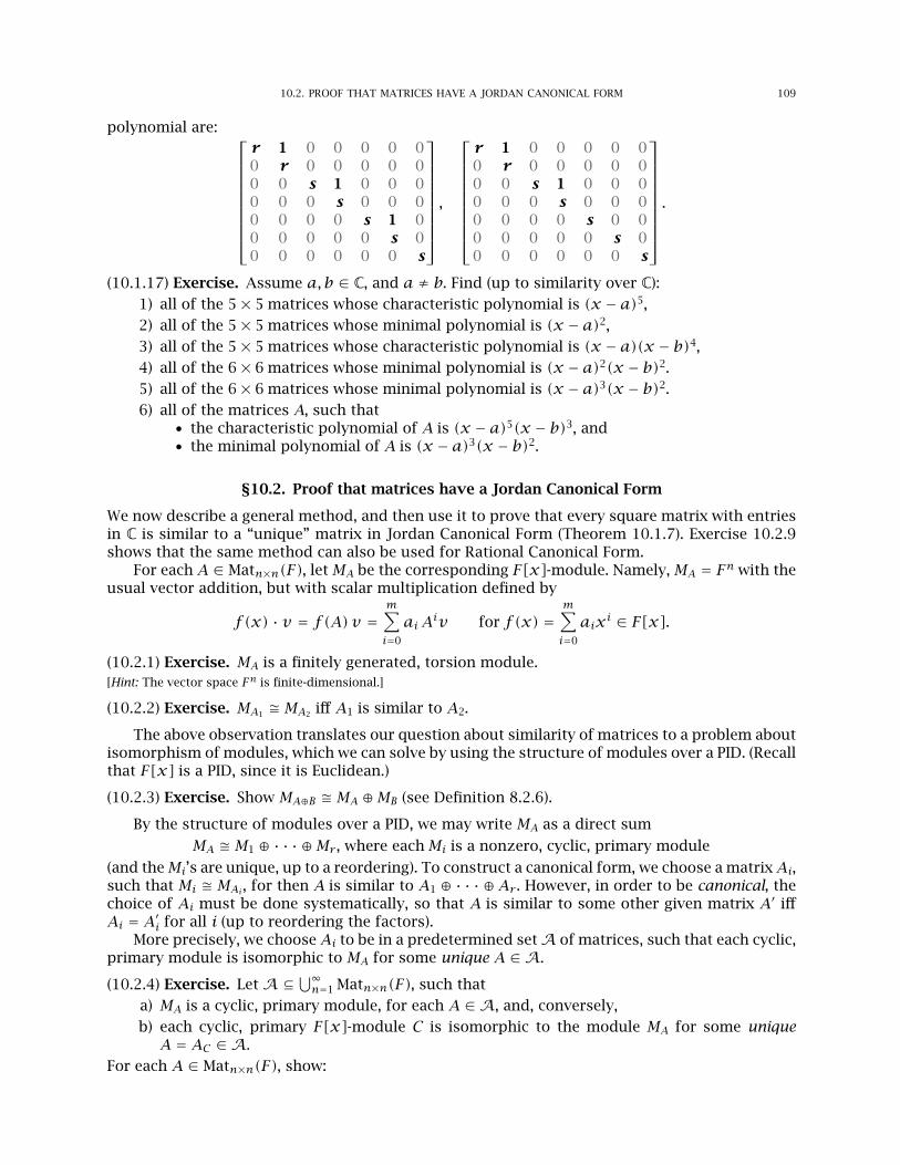
10.2. PROOF THAT MATRICES HAVE A JORDAN CANONICAL FORM 109
polynomial are:
r 1 0 0 0 0 00 r 0 0 0 0 00 0 s 1 0 0 00 0 0 s 0 0 00 0 0 0 s 1 00 0 0 0 0 s 00 0 0 0 0 0 s
,
r 1 0 0 0 0 00 r 0 0 0 0 00 0 s 1 0 0 00 0 0 s 0 0 00 0 0 0 s 0 00 0 0 0 0 s 00 0 0 0 0 0 s
.
(10.1.17) Exercise. Assume a,b ∈ C, and a ≠ b. Find (up to similarity over C):1) all of the 5× 5 matrices whose characteristic polynomial is (x − a)5,2) all of the 5× 5 matrices whose minimal polynomial is (x − a)2,3) all of the 5× 5 matrices whose characteristic polynomial is (x − a)(x − b)4,4) all of the 6× 6 matrices whose minimal polynomial is (x − a)2(x − b)2.5) all of the 6× 6 matrices whose minimal polynomial is (x − a)3(x − b)2.6) all of the matrices A, such that
• the characteristic polynomial of A is (x − a)5(x − b)3, and• the minimal polynomial of A is (x − a)3(x − b)2.
§10.2. Proof that matrices have a Jordan Canonical Form
We now describe a general method, and then use it to prove that every square matrix with entriesin C is similar to a “unique” matrix in Jordan Canonical Form (Theorem 10.1.7). Exercise 10.2.9shows that the same method can also be used for Rational Canonical Form.
For each A ∈ Matn×n(F), letMA be the corresponding F[x]-module. Namely,MA = Fn with theusual vector addition, but with scalar multiplication defined by
f(x) · v = f(A)v =m∑i=0
aiAiv for f(x) =m∑i=0
aixi ∈ F[x].
(10.2.1) Exercise. MA is a finitely generated, torsion module.[Hint: The vector space Fn is finite-dimensional.]
(10.2.2) Exercise. MA1 ≊ MA2 iff A1 is similar to A2.
The above observation translates our question about similarity of matrices to a problem aboutisomorphism of modules, which we can solve by using the structure of modules over a PID. (Recallthat F[x] is a PID, since it is Euclidean.)
(10.2.3) Exercise. Show MA⊕B ≊ MA ⊕MB (see Definition 8.2.6).
By the structure of modules over a PID, we may write MA as a direct sum
MA ≊ M1 ⊕ · · · ⊕Mr , where eachMi is a nonzero, cyclic, primary module
(and theMi’s are unique, up to a reordering). To construct a canonical form, we choose a matrixAi,such that Mi ≊ MAi, for then A is similar to A1 ⊕ · · · ⊕Ar . However, in order to be canonical, thechoice of Ai must be done systematically, so that A is similar to some other given matrix A′ iffAi = A′i for all i (up to reordering the factors).
More precisely, we choose Ai to be in a predetermined setA of matrices, such that each cyclic,primary module is isomorphic to MA for some unique A ∈A.
(10.2.4) Exercise. Let A⊆ ⋃∞n=1 Matn×n(F), such thata) MA is a cyclic, primary module, for each A ∈A, and, conversely,b) each cyclic, primary F[x]-module C is isomorphic to the module MA for some uniqueA = AC ∈A.
For each A ∈ Matn×n(F), show:
110 10. JORDAN CANONICAL FORM
1) A is similar to A1 ⊕ · · · ⊕Ar , for some A1, . . . , Ar ∈A (and some r).
2) r and A1, . . . , Ar are unique (up to a reordering).
3) Suppose A′ is similar to A′1 ⊕ · · · ⊕ A′s, with A′1, . . . , A′s ∈ A. Then the matrices A and A′are similar if and only if r = s and, after a reordering, we have Ai = A′i for every i.
Now, let’s prove Theorem 10.1.7 (Jordan Canonical Form) by establishing the hypotheses ofExercise 10.2.4.
(10.2.5) Proposition. IfA = Jk(a), for some a ∈ Cand k ∈ N+, then the correspondingC[x]-moduleMA is cyclic, torsion, and primary.
Proof. (cyclic) For simplicity, we first consider the case where a = 0, which means A = Jk(0). Let{e1, . . . , ek} be the standard basis of Ck, and note that the columns of Jk(0) are (from left to right):
0, e1, e2, . . . , ek−1,so the ith column of Jk(0) is ei−1, for i ≥ 2. This means
Aei = Jk(0)ei = ei−1 for 2 ≤ i ≤ k.Hence, for v = ek, we see, by induction on i, that Aiv = ek−i for 0 ≤ i < k. Hence
C[x]v ⊃ ⟨Aiv | 0 ≤ i < k ⟩ = ⟨ ek, ek−1, ek−2, . . . , e2, e1 ⟩ = Ck,since {e1, . . . , ek} is a basis. So MA is cyclic.
Essentially the same proof applies in the general case, because
⟨ Jk(0)i v | 0 ≤ i < k ⟩ ⊆ C[x]v,since Jk(0)i = (A− aI)i ∈ C[A].
(torsion and primary) Let f(x) = (x − a)k, so
f(A) = (A− aI)k = (Jk(a)− aI)k = Jk(0)k = 0.Then f(x) annihilates MA (since, for any m ∈ MA, we have f(x)m = f(A)m = 0m = 0). Sincef(x) is a power of the irreducible polynomial x−a, this implies thatMA is torsion and primary. □
(10.2.6) Exercise. Conversely, if M is a nonzero, cyclic, primary, torsion module over C[x], thenM ≊ MJk(a), for some a ∈ C and k ∈ N+.[Hint: By assumption, M is cyclic, and its annihilator is C[x]π(x)k, for some irreducible polynomial π(x) ∈ C[x], andsome k ∈ N+. The Fundamental Theorem of Algebra (8.2.16) tells us that p(x) has a root a in C, which means that p(x) isdivisible by the linear polynomial x−a. So irreducibility implies that π(x) is x−a (times a unit). Then the cyclic modulesM and MJk(a) have the same annihilator, so they are isomorphic.]
(10.2.7) Proposition. Suppose k,ℓ ∈ N+ and a,b ∈ C. If MJk(a) ≊ MJℓ(b), then k = ℓ and a = b.
Proof. The assumption implies that Jk(a) is similar to Jℓ(b) (see Exercise 10.2.2). Since Jk(a) is ak × kmatrix and Jℓ(b) is an ℓ × ℓmatrix, this implies k = ℓ. It also implies that Jk(a) and Jℓ(b)have the same eigenvalues (cf. Remark 8.3.10). Since a is the only eigenvalue of Jk(a), and b is theonly root of eigenvalue of Jℓ(b), we conclude that a = b. □
Proof of Theorem 10.1.7. Combining Propositions 10.2.5 and 10.2.7 and Exercise 10.2.6 showsthat the set J of Jordan blocks Jk(λ) satisfies the hypotheses of Exercise 10.2.4. This establishesthat every matrix is similar to a matrix that is in Jordan Canonical Form (and that the blocks areunique, up to a permutation). □
(10.2.8) Remark. Although we have only discussed matrices whose entries are complex numbers,the same ideas apply more generally. Namely, suppose A ∈ Matn×n(F), where F is any field. Thenthe above line of reasoning can be used to show that A is similar to a matrix in Jordan CanonicalForm if and only if every eigenvalue of A is in F. (In other words, if and only if the characteristicpolynomial of A factors as a product of linear polynomials in F[x].)
We close the section with another important application of Exercise 10.2.4:

10.2. PROOF THAT MATRICES HAVE A JORDAN CANONICAL FORM 111
(10.2.9) Exercise. For f(x) = xn + an−1xn−1 + · · · + a1x + a0 ∈ F[x], we use Af to denote thecompanion matrix of f(x), which means
Af =
0 0 0 · · · 0 −a0
1 0 0 · · · 0 −a1
0 1 0 · · · 0 −a2
0 0 1 · · · 0 −a3...
......
. . ....
...0 0 0 · · · 1 −an−1
.
Show:1) The minimal polynomial and characteristic polynomial of Af are f(x).2) The F[x]-module corresponding to Af is isomorphic to F[x]/⟨f(x)⟩.
[Hint: Exercise 6.3.5(9).]
3) Any n×nmatrix A over F is similar to a matrix of the form
Af1 ⊕Af2 ⊕ · · · ⊕Afk ,where
each fi is a power of a monic irreducible polynomial.Furthermore, the choice of f1, f2, . . . , fk is unique (up to a permutation).
4) (Rational Canonical Form) The same as the preceding, except we change the assumptionon fi to:
fi is a divisor of fi+1 for every i (and no fi is a unit).However, in this case, the choice of f1, f2, . . . , fk is entirely unique (not merely up topermutations).

Index
π-primary, 70π-primary component, 70
abelian, 4acc, 53, 74action by automorphisms, 45action of a group, 19adjoint, 92, 95, 97algebra, 85algebraic number theory, 55alternating group, 36annihilator, 63ascending central series, 34ascending chain condition, 53, 74associates, 52automorphism, 16, 51Axiom of Choice, 78
basis, 66, 67, 83bijection, 8bilinear form, 93binomial coefficient, 23block-diagonal, 86
cardinality, 3Cauchy’s Theorem, 25Cayley’s Theorem, 19Cayley-Hamilton Theorem, 107central series, 30centralizer, 12centralizes, 4centre, 12chain, 77chain generated by b, 79change-of-basis matrix, 84characteristic polynomial, 86characteristic subgroup, 28class equation, 22commutative, 50commutative diagram, 43commutative group, 4commutator, 28commutator subgroup, 28commute, 4composition, 8composition factors, 37composition series, 36conjugacy class, 22conjugate, 13, 92, 97conjugate-transpose, 92
conjugation, 56conjugation by g, 16coordinates, 84Correspondence Theorem, 17, 52, 65cycle, 8cyclic, 12cyclic module, 63cyclic subgroup, 12
dcc, 54degree, 57derived group, 29derived series, 29descending central series, 34descending chain condition, 54determinant, 85, 86dihedral group, 7dimension, 84direct product, 5, 44, 67direct product (internal), 33direct sum, 50, 64, 67direct sum (internal), 64, 68disjoint, 8dot product, 92double-dual, 95dual basis, 95dual space, 94
eigenspace, 86eigenvalue, 86eigenvector, 86Euclidean domain, 52
Fermat’s Little Theorem, 25field, 53finite-dimensional vector space, 83fixed point, 9, 24Frattini argument, 32Frattini subgroup, 32free, 67free group, 42free module, 64, 66Fundamental Theorem of Algebra, 88Fundamental Theorem of Finite Abelian Groups, 75Fundamental Theorem of Finitely Generated Abelian
Groups, 69
gcd, 54generates, 13generating set, 13, 63
113
114 INDEX
generators and relations, 39, 44Gram-Schmidt Orthogonalization, 98greatest common divisor, 54group, 3
Hermitian form, 92, 97homomorphism, 15, 51, 63
ideal, 50identity map, 9image, 8, 63index of a subgroup, 14initial segment, 79injective, 7inner automorphism, 16integers modulo n, 5integral domain, 52irreducible, 52isomorphic, 15, 51, 63isomorphism, 15, 51, 63Isomorphism Theorems (1st, 2nd, and 3rd), 16, 52, 65ith derived group G(i), 29
Jordan block, 106Jordan Canonical Form, 106Jordan-Hölder Theorem, 37
k-cycle, 8kernel, 15, 51, 63kernel of a group action, 19kernel of a homomorphism, 19Klein bottle group, 45
Lagrange’s Theorem, 14left coset, 14left ideal, 50length of a composition series, 36length of a vector, 96, 97linear, 57Linear Algebra, 83linear combination, 66, 67, 83linear functional, 94linear operator, 83linear transformations, 83linearly independent, 66, 67, 83lower central series, 34
maximal, 55maximal element, 77maximal subgroup, 31maximal submodule, 65minimal normal subgroup, 30minimal polynomial, 89module, 61monic polynomial, 86
nilpotence class, 35nilpotent, 90nilpotent group, 30no torsion, 69Noetherian, 53, 74nondegenerate, 94, 97nontrivial subgroup, 12nonzero, 50nonzero ring, 53
norm, 52, 56norm of a vector, 96, 97normal, 98normal series, 29normal subgroup, 13normalizer, 12normalizes, 13number theory, 55
one-to-one, 7onto, 8orbit, 20Orbit-Stabilizer Theorem, 21order, 4orthogonal complement, 98orthogonal matrix, 91orthonormal, 98
p-group, 23p-subgroup, 23partial order, 77partially ordered set, 77partition, 14, 20, 76Pell Equation, 55perfect group, 30permutation, 8PID, 52polynomial, 57positive-definite, 98power set, 20presentation, 39primary, 70primary component, 70prime, 53principal, 52principal ideal domain, 52proper, 50proper subgroup, 12proper submodule, 62pure, 100
quotient, 14, 62quotient ring, 50quotients (of a subnormal series), 29
R-module, 61rank, 71Rational Canonical Form, 111reduced word, 43refinement, 36regular R-module, 61regular action, 19relation, 39repeated root, 59restricting an action to a subgroup, 20right coset, 14right ideal, 50ring, 49ring of polynomials over F, 58root, 58
same cardinality, 8self-adjoint, 98self-normalizing, 31
INDEX 115
semidirect product, 5, 45semidirect product (internal), 45similar, 85, 105simple group, 36simple module, 65solvable group, 29spanning set, 66, 67spans, 66, 67, 83Spectral Theorem, 98square-free, 46stabilizer, 20standard basis, 83Structure Theorem for Finitely Generated Modules over
a PID, 69subgroup, 12subgroup generated by S, 13submodule, 62submodule generated by S, 63subnormal series, 29subring, 50subspaces, 83supersolvable, 35surjective, 8Sylow p-subgroup, 23Sylow subgroup, 23Sylow Theorems, 23Sylp(G), 23symmetric, 91, 96, 99symmetric group, 8symmetric group on n letters, 8symmetry, 5
T-invariant, 90tensor product, 100torsion, 69torsion-free, 69totally ordered, 77trace, 102transfinite induction, 77transitive action, 20transpose, 91, 95triangularizable, 87trivial action, 20trivial subgroup, 12trivial submodule, 62two-sided ideal, 50
UFD, 52unique factorization domain, 52unit, 52unitary, 98, 99upper bound, 77upper central series, 34upper-triangular, 85
vector spaces, 83Von Dyck’s Theorem, 40
well-ordered, 53, 79without repetition, 36word problem, 42
zero, 50zero divisor, 52
zero of a polynomial, 58zero polynomial, 57zero ring, 53Zorn’s Lemma, 77
![A logical approach to abstract algebra - Chalmerscoquand/pml.pdfA logical approach to abstract algebra A logical approach to abstract algebra [19] Serre’s splitting-off theorem](https://img.pdfslide.us/doc/110x75/611ee3c6e577f259fa14ae50/a-logical-approach-to-abstract-algebra-coquandpmlpdf-a-logical-approach-to-abstract.jpg)