Embed Size (px)
Citation preview
Abstract AlgebraEdition 2.71

Abstract Algebraby
Justin R. Smith

This is dedicated to mywonderful wife, Brigitte.
c©2020. Justin R. Smith. All rights reserved.
ISBN: 9798579698353 (KDP-assigned) paperback
Also published by Five Dimensions Press Introduction to Algebraic Geometry (paperback and hardcover),
Justin Smith. Eye of a Fly (Kindle edition and paperback), Justin Smith. The God Virus, (Kindle edition and paperback) by Justin Smith. Ohana, (Kindle edition and paperback) by Justin Smith. The Accidental Empress, (Kindle edition and paperback) by Justin
Smith. Die zufällige Kaiserin, German translation of The Accidental Empress
(Kindle edition and paperback) by Justin Smith.
Five Dimensions Press page:HTTP://www.five-dimensions.org
Email:[email protected]


Foreword
Algebra is the offer made by the devil to the mathematician. Thedevil says “I will give you this powerful machine, and it will an-swer any question you like. All you need to do is give me yoursoul; give up geometry and you will have this marvelous ma-chine.”
M. F. Atiyah (2001)
This book arose out of courses in Abstract Algebra, Galois Theory, Al-gebraic Geometry, and Manifold Theory the author taught at Drexel Uni-versity.
It is useful for self-study or as a course textbook.The first four chapters are suitable for the first of a two semester un-
dergraduate course in Abstract Algebra and chapters five through sevenare suitable for the second semester.
Chapter 2 on page 5 covers a few preliminaries on basic set theory (ax-iomatic set theory is discussed in appendix A on page 459).
Chapter 3 on page 13 discusses basic number theory, which is a use-ful introduction to the theory of groups. It also presents an application ofnumber theory to cryptography.
Chapter 4 on page 33 discusses the theory of groups and homomorph-isms of groups.
Chapter 5 on page 107 covers ring-theory with material on computa-tions in polynomial rings and Gröbner bases. It also discusses some appli-cations of algebra to motion-planning and robotics.
Chapter 6 on page 161 covers basic linear algebra, determinants, anddiscusses modules as generalizations of vector-spaces. We also discuss re-sultants of polynomials and eigenvalues.
Chapter 7 on page 259 discusses basic field-theory, including algebraicand transcendental field-extensions, finite fields, and the unsolvability ofsome classic problems in geometry. This, section 4.9 on page 84, and chap-ter 8 on page 295 might be suitable for a topics course in Galois theory.
Chapter B on page 465 discusses some more advanced areas of the the-ory of rings, like Artinian rings and integral extensions.
Chapter 8 on page 295 covers basic Galois Theory and should be readin conjunction with chapter 7 on page 259 and section 4.9 on page 84.
Chapter 9 on page 321 discusses division-algebras over the realnumbers and their applications. In particular, it discusses applicationsof quaternions to computer graphics and proves the Frobenius Theoremclassifying associative division algebras over the reals. It also developsoctonions and discusses their properties.
vii
Chapter 10 on page 335 gives an introduction to Category Theory andapplies it to concepts like direct and inverse limits and multilinear algebra(tensor products an exterior algebras).
Chapter 11 on page 383 gives a brief introduction to group representa-tion theory.
Chapter 12 on page 411 gives a brief introduction to algebraic geometryand proves Hilbert’s Nullstellensatz.
Chapter 13 on page 429 discusses some 20th century mathematics: ho-mology and cohomology. It covers chain complexes and chain-homotopyclasses of maps and culminates in a little group-cohomology, including theclassification of abelian extensions of groups.
Sections marked in this manner are more advanced or specialized and maybe skipped on a first reading.
Sections marked in this manner are even more advanced or specializedand may be skipped on a first reading (or skipped entirely).
I am grateful to Matthias Ettrich and the many other developers ofthe software, LYX — a free front end to LATEX that has the ease of use ofa word processor, with spell-checking, an excellent equation editor, and athesaurus. I have used this software for years and the current version ismore polished and bug-free than most commercial software.
I am grateful to Darij Grinberg for his extremely careful reading of themanuscript. He identified several significant errors. I would also like tothank Xintong Li for pointing out errors in some of my definitions.
LYX is available from HTTP://www.lyx.org.Edition 2.7: I have added material on the classification of modules over
a principal ideal domain and the Jordan Canonical Form, as well as an ex-panded section on quaternions, octonions and sedenions.
Edition 2.71: I have added material on group representation theory.
Contents
Foreword vii
List of Figures xiii
Chapter 1. Introduction 1
Chapter 2. Preliminaries 52.1. Numbers 52.2. Set theory 92.3. Operations on sets 102.4. The Power Set 11
Chapter 3. A glimpse of number theory 133.1. Prime numbers and unique factorization 133.2. Modular arithmetic 183.3. The Euler φ-function 213.4. Applications to cryptography 253.5. Quadratic Residues 26
Chapter 4. Group Theory 334.1. Introduction 334.2. Homomorphisms 394.3. Cyclic groups 404.4. Subgroups and cosets 434.5. Symmetric Groups 494.6. Abelian Groups 584.7. Group-actions 734.8. The Sylow Theorems 804.9. Subnormal series 844.10. Free Groups 874.11. Groups of small order 104
Chapter 5. The Theory of Rings 1075.1. Basic concepts 1075.2. Homomorphisms and ideals 1115.3. Integral domains and Euclidean Rings 1175.4. Noetherian rings 1215.5. Polynomial rings 1255.6. Unique factorization domains 1455.7. The Jacobson radical and Jacobson rings 154
ix
x CONTENTS
5.8. Artinian rings 157
Chapter 6. Modules and Vector Spaces 1616.1. Introduction 1616.2. Vector spaces 1636.3. Modules 2206.4. Rings and modules of fractions 2466.5. Integral extensions of rings 249
Chapter 7. Fields 2597.1. Definitions 2597.2. Algebraic extensions of fields 2637.3. Computing Minimal polynomials 2707.4. Primitive roots of unity 2747.5. Algebraically closed fields 2817.6. Finite fields 2857.7. Transcendental extensions 289
Chapter 8. Galois Theory 2958.1. Before Galois 2958.2. Galois 2988.3. Isomorphisms of fields 2988.4. Roots of Unity 3018.5. Group characters 3028.6. Galois Extensions 3068.7. Solvability by radicals 3128.8. Galois’s Great Theorem 3158.9. The fundamental theorem of algebra 319
Chapter 9. Division Algebras over R 3219.1. The Cayley-Dickson Construction 3219.2. Quaternions 3239.3. Octonions and beyond 330
Chapter 10. A taste of category theory 33510.1. Introduction 33510.2. Functors 34110.3. Adjoint functors 34510.4. Limits 34710.5. Abelian categories 35710.6. Direct sums and Tensor products 36110.7. Tensor Algebras and variants 374
Chapter 11. Group Representations, a Drive-by 38311.1. Introduction 38311.2. Finite Groups 38911.3. Characters 39411.4. Examples 40511.5. Burnside’s Theorem 407

CONTENTS xi
Chapter 12. A little algebraic geometry 41112.1. Introduction 41112.2. Hilbert’s Nullstellensatz 41512.3. The coordinate ring 423
Chapter 13. Cohomology 42913.1. Chain complexes and cohomology 42913.2. Rings and modules 44313.3. Cohomology of groups 450
Appendix A. Axiomatic Set Theory 459A.1. Introduction 459A.2. Zermelo-Fraenkel Axioms 459
Appendix B. Further topics in ring theory 465B.1. Discrete valuation rings 465B.2. Metric rings and completions 469B.3. Graded rings and modules 469
Appendix. Glossary 519
Appendix. Index 521
Appendix. Bibliography 529

List of Figures
2.1.1 The real line, R 62.1.2 The complex plane 9
4.1.1 The unit square 364.1.2 Symmetries of the unit square 364.5.1 Regular pentagon 584.7.1 A simple graph 74
5.4.1 Relations between classes of rings 1235.5.1 Reaching a point 1385.5.2 Points reachable by the second robot arm 140
6.2.1 Image of a unit square under a matrix 1896.2.2 A simple robot arm 2026.2.3 A more complicated robot arm 2036.2.4 Projection of a vector onto another 2086.2.5 The plane perpendicular to u 211
6.2.6 Rotation of a vector in R3 212
9.3.1 Fano Diagram 331
12.1.1 An elliptic curve 41212.1.2 Closure in the Zariski topology 41412.2.1 An intersection of multiplicity 2 420
xiii

Abstract AlgebraEdition 2.71

CHAPTER 1
Introduction
“L’algèbre n’est qu’une géométrie écrite; la géométrie n’estqu’une algèbre figurée.” (Algebra is merely geometry in words;geometry is merely algebra in pictures)
— Sophie Germain, [44]
The history of mathematics is as old as that of human civilization itself.Ancient Babylon (circa 2300 BCE) used a number-system that was surpris-ingly modern except that it was based on 60 rather than 10 (and still lackedthe number 0). This is responsible the fact that a circle has 360 and for ourtime-units, where 60 seconds form a minute and 60 minutes are an hour.The ancient Babylonians performed arithmetic using pre-calculated tablesof squares and used the fact that
ab =(a + b)2 − a2 − b2
2
to calculate products. Although they had no algebraic notation, they knewabout completing the square to solve quadratic equations and used tablesof squares in reverse to calculate square roots.
In ancient times, mathematicians almost always studied algebra in itsguise as geometry — apropos of Sophie Germain’s quote. Ancient Greekmathematicians solved quadratic equations geometrically, and the greatPersian poet-mathematician, Omar Khayyam1, solved cubic equations thisway.
Geometry in the West originated in Egypt, where it began as a kind offolk-mathematics farmers used to survey their land after the Nile’s annualflooding (the word geometry means “earth measurement” in Greek). Themore advanced geometry used in building pyramids remained the secretof the Egyptian priesthood.
The Greek merchant2 and amateur mathematician, Thales, traveled toEgypt and paid priests to learn about geometry.
Thales gave the first proof of a what was a well-known theorem ingeometry. In general, Greece’s great contribution to mathematics was inthe concept of proving that statements are true. This arose from many of theearly Greek mathematicians being lawyers.
In ancient Greek geometry, there were a number of famous problemsthe ancient Greeks couldn’t solve: squaring the circle (finding a square
1The Omar Khayyam who wrote the famous poem, The Rubaiyat — see [39].2He is credited with the first recorded use of financial arbitrage.
1
2 1. INTRODUCTION
whose area was the same as a given circle), doubling a cube (given a cube,construct one with double its volume), and trisecting an angle.
It turned out that these problems have no solutions, although prov-ing that required modern algebra and number theory (see chapter 7 onpage 259).
Ancient India had a sophisticated system of mathematics that remainslargely unknown since it was not written down3. Its most visible mod-ern manifestation is the universally used decimal number system and es-pecially, the number zero. Otherwise, Indian mathematics is known forisolated, deep results given without proof, like the infinite series
π
4= 1− 1
3+
15− 1
7+ · · ·
Arabic mathematicians transmitted Indian numerals to Europeand originated what we think of as algebra today — i.e. the use ofnon-geometric abstract symbols. One of the first Arabic texts describescompleting the square in a quadratic equation in verbal terms4.
There are hints of developments in Chinese mathematics from 1000B.C.E. — including decimal, binary, and negative numbers. Most of thiswork was destroyed by the order of First Emperor of the Qin dynasty, QinShi Huangdi, in his Great Book Burning.
Isolated results like the Chinese Remainder Theorem (see 3.3.5 onpage 24) suggest a rich mathematical tradition in ancient China. TheJiuzhang suanshu or, the Nine Chapters on the Mathematical Art, from 200B.C.E., solves systems of three linear equations in three unknowns. This isthe beginning of linear algebra (see chapter 6 on page 161)
The ancient Greeks regarded algebraic functions in purely geometricterms: a square of a number was a physical square and a numbers’ cubewas a physical cube. Other exponents had no meaning for them.
The early European view of all things as machines changed that: num-bers became idea-machines, whose properties did not necessarily have anyphysical meaning. Nicole Oresme had no hesitation in dealing with pow-ers other than 2 and 3 or even fractional exponents. This led to entirely newapproaches to algebra.
Nicole Oresme, (1320 – 1382) was a French philosopher, astrologer, andmathematician. His main mathematical work, Tractatus de configurationibusqualitatum et motuum, was a study on heat flow. He also proved the diver-gence of the harmonic series.
After Oresme, Renaissance Europe saw the rise of the concept of virtù— not to be confused with “virtue”. The hero with virtù was competentin all things — and notable figures conducted public displays of skills likeswordsmanship, poetry, art, chess, or . . . mathematics. Tartaglia’s solutionof the general cubic equation was originally written in a poem.
3It was passed from teacher to student in an oral tradition.4This makes one appreciate mathematical notation!
1. INTRODUCTION 3
Bologna University, in particular, was famed for its intense publicmathematics competitions.
People often placed bets on the outcome, rewarding winners with fi-nancial prizes. These monetary rewards motivated a great deal of mathe-matical research. Like magicians, mathematicians often kept their researchsecret — as part of their “bag of tricks5.”
Renaissance Italy also saw the solution of the general quartic (i.e.,fourth degree) equation — see section 8.1 on page 295. Attempts to pushthis further — to polynomials of degree five and higher — failed. In theearly 1800’s Abel and Galois showed that it is impossible — see chapter 8on page 295.
The nineteenth and twentieth centuries saw many developments inalgebra, often motivated by algebraic geometry and topology. See chap-ters 12 on page 411 and 13 on page 429.
5Tartaglia told Cardano his solution to the general cubic equation and swore him to strictsecrecy. When Cardano published this solution, it led to a decade-long rift between the twomen.

CHAPTER 2
Preliminaries
“The number system is like human life. First you have the naturalnumbers. The ones that are whole and positive. Like the num-bers of a small child. But human consciousness expands. Thechild discovers longing. Do you know the mathematical expres-sion for longing? The negative numbers. The formalization of thefeeling that you’re missing something. Then the child discoversthe in between spaces, between stones, between people, betweennumbers and that produces fractions, but it’s like a kind of mad-ness, because it does not even stop there, it never stops. . . Math-ematics is a vast open landscape. You head towards the horizonand it’s always receding. . . ”
— Smilla Qaavigaaq Jaspersen, in the novel Smilla’s Sense ofSnow, by Peter Høeg (see [57]).
2.1. Numbers
The natural numbers, denoted N, date back to prehistoric times. Theyare numbers
1, 2, 3, . . .Now we go one step further. The integers, denoted Z, include the natu-
ral numbers, zero, and negative numbers. Negative numbers first appearedin China in about 200 BCE.
Zero as a digit (i.e., a place-holder in a string of digits representing anumber) appears to date back to the Babylonian culture, which denoted itby a space or dot. Zero as a numerical value seems to have originated in In-dia around 620 AD in a work of Brahmagupta that called positive numbersfortunes and negative numbers debts. This work also correctly stated therules for multiplying and dividing positive and negative numbers, exceptthat it stated 0/0 = 0.
So we have the integers:
Z = . . . .− 3,−2,−1, 0, 1, 2, 3, . . . The next step involves fractions and the rational number system. Fractions(positive ones, at least) have appeared as early as ancient Egypt with nu-merators that were always 1. For instance, the fraction
83
would be represented in ancient Egypt as
2 +12+
16
5
6 2. PRELIMINARIES
−3 −2 −1 0 1 2 3
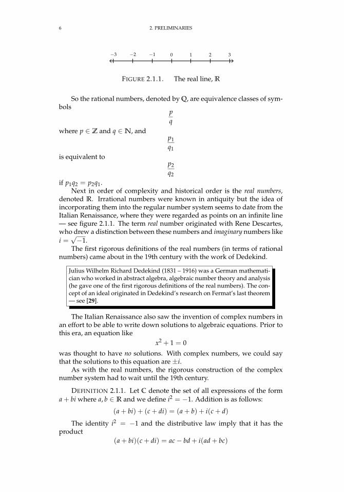
FIGURE 2.1.1. The real line, R
So the rational numbers, denoted by Q, are equivalence classes of sym-bols
pq
where p ∈ Z and q ∈N, andp1
q1
is equivalent top2
q2
if p1q2 = p2q1.Next in order of complexity and historical order is the real numbers,
denoted R. Irrational numbers were known in antiquity but the idea ofincorporating them into the regular number system seems to date from theItalian Renaissance, where they were regarded as points on an infinite line— see figure 2.1.1. The term real number originated with Rene Descartes,who drew a distinction between these numbers and imaginary numbers likei =√−1.
The first rigorous definitions of the real numbers (in terms of rationalnumbers) came about in the 19th century with the work of Dedekind.
Julius Wilhelm Richard Dedekind (1831 – 1916) was a German mathemati-cian who worked in abstract algebra, algebraic number theory and analysis(he gave one of the first rigorous definitions of the real numbers). The con-cept of an ideal originated in Dedekind’s research on Fermat’s last theorem— see [29].
The Italian Renaissance also saw the invention of complex numbers inan effort to be able to write down solutions to algebraic equations. Prior tothis era, an equation like
x2 + 1 = 0
was thought to have no solutions. With complex numbers, we could saythat the solutions to this equation are ±i.
As with the real numbers, the rigorous construction of the complexnumber system had to wait until the 19th century.
DEFINITION 2.1.1. Let C denote the set of all expressions of the forma + bi where a, b ∈ R and we define i2 = −1. Addition is as follows:
(a + bi) + (c + di) = (a + b) + i(c + d)
The identity i2 = −1 and the distributive law imply that it has theproduct
(a + bi)(c + di) = ac− bd + i(ad + bc)
2.1. NUMBERS 7
where a + bi, c + di ∈ R2 = C. It is not hard to see that 1 is the identityelement of C. Given z = a + bi ∈ C, define <(z) = a and =(z) = b, the realand imaginary parts, respectively.
If x = a + bi, the complex conjugate of x, denoted x, is a− bi. Then
x · x = a2 + b2 ∈ R
and
(a + bi)(
aa2 + b2 −
bia2 + b2
)= 1
so
(2.1.1) (a + bi)−1 =a
a2 + b2 −bi
a2 + b2
If x = a + bi, the quantity |x| =√
x · x =√
a2 + b2 is called the absolutevalue of x. Note that |x| = 0 implies that x = 0.
REMARK. Complex numbers can represent points in the plane and onecan add, subtract, multiply, and divide them (see section 9.1 on page 321).Note that complex multiplication is associative and commutative (left to thereader to prove!):
z1(z2z3) = (z1z2)z3
z1z2 = z2z1
for zi ∈ C.
Leonhard Euler (1707 – 1783) was, perhaps, the greatest mathematician alltime. Although he was born in Switzerland, he spent most of his life in St.Petersburg, Russia and Berlin, Germany. He originated the notation f (x)for a function and made contributions to mechanics, fluid dynamics, optics,astronomy, and music theory. His final work, “Treatise on the Constructionand Steering of Ships,” is a classic whose ideas on shipbuilding are stillused to this day.
To do justice to Euler’s life would require a book considerably longerthan the current one — see the article [42]. His collected works fill morethan 70 volumes and, after his death, he left enough manuscripts behindto provide publications to the Journal of the Imperial Academy of Sciences(of Russia) for 47 years.
One of his many accomplishments is:
THEOREM 2.1.2 (Euler’s Formula). If x ∈ R, then
(2.1.2) eix = cos(x) + i sin(x)
PROOF. Just plug ix into the power series for exponentials
(2.1.3) ey = 1 + y +y2
2!+
y3
3!+ · · ·
8 2. PRELIMINARIES
to get
eix = 1 + ix− x2
2!− i
x3
3!+ · · ·
=
(1− x2
2!+
x4
4!− · · ·
)+ i(
x− x3
3!+
x5
5!− · · ·
)= cos x + i sin x
Since x = cos(θ), y = sin(θ) is the parametric equation of a circle, itfollows that all points on the unit circle in C are of the form eiθ for a suitableθ. If we draw a line from the origin to a point, u, on the unit circle, θ is theangle it makes with the real axis.
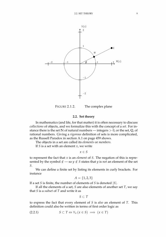
If z ∈ C is an arbitrary nonzero element, u = z/|z| is on the unit circle,so u = eiθ and
z = |z| · eiθ
— see figure 2.1.2 on the facing page.For instance, if z = 2 + i, we have |z| =
√5 and
u =1√5(2 + i) = eiθ
whereθ = arctan(1/2)
If we multiply z by eiφ, we get
zeiφ = |z| · ei(θ+φ)
which now makes an angle of θ + φ with the real axis. It follows that mul-tiplication has a geometric significance:
Multiplying by eiφ rotates the entire complex plane in acounterclockwise direction by φ.
The complex numbers transformed entire fields of mathematics, in-cluding function theory, number theory, and early topology. Doing thesedevelopments justice would fill several books larger than the current vol-ume.
EXERCISES.
1. If x, y ∈ C, show that x · y = x · y.
2. If x, y ∈ C, show that |x| · |y| = |x · y|.
2.2. SET THEORY 9
<z
=z
−2
−2
−1
−1
1
1
2
2
z
uu
θ
FIGURE 2.1.2. The complex plane
2.2. Set theory
In mathematics (and life, for that matter) it is often necessary to discusscollections of objects, and we formalize this with the concept of a set. For in-stance there is the set N of natural numbers — integers > 0, or the set, Q, ofrational numbers. Giving a rigorous definition of sets is more complicated,as the Russell Paradox in section A.1 on page 459 shows.
The objects in a set are called its elements or members.If S is a set with an element x, we write
x ∈ S
to represent the fact that x is an element of S. The negation of this is repre-sented by the symbol /∈— so y /∈ S states that y is not an element of the setS.
We can define a finite set by listing its elements in curly brackets. Forinstance
A = 1, 2, 3If a set S is finite, the number of elements of S is denoted |S|.
If all the elements of a set, S are also elements of another set T, we saythat S is a subset of T and write it as
S ⊂ T
to express the fact that every element of S is also an element of T. Thisdefinition could also be written in terms of first order logic as
(2.2.1) S ⊂ T ⇔ ∀x (x ∈ S) =⇒ (x ∈ T)

10 2. PRELIMINARIES
where the symbol ∀x means “for all possible values of x”.Note that every set is a subset of itself, so S ⊂ S.The empty set is denoted ∅ — it contains no elements. Equation 2.2.1 on
the preceding page implies that for any set, S,
∅ ⊂ S
2.3. Operations on sets
We can perform various operations on setsUnion: If A and B are sets, their union — written A ∪ B — consists of all
elements of A and all elements of B.Example: If A = 1, 2, 3 and B = 1, 6, 7, then
A ∪ B = 1, 2, 3, 6, 7We could give a first-order logic definition of union via
∀xx ∈ A ∪ B⇔ (x ∈ A) ∨ (x ∈ B)
In some sense, the union operation is a set-version of the logical oroperation.
Intersection: If A and B are sets, their intersection — written A ∩ B — con-sists of all elements contained in both A and B.
Example: If A = 1, 2, 3 and B = 1, 6, 7, then
A ∩ B = 1We could give a first-order logic definition of union via
∀xx ∈ A ∩ B⇔ (x ∈ A) ∧ (x ∈ B)
In some sense, the intersection operation is a set-version of the log-ical and operation.
Difference: If A and B are sets, their difference — written A \ B — consistsof all elements of A not also in B.
Example: If A = 1, 2, 3 and B = 1, 6, 7, then
A \ B = 2, 3We could give a first-order logic definition of union via
∀xx ∈ A \ B⇔ (x ∈ A) ∧ (x /∈ B)
Complement: If A is a set Ac or A denotes its complement — all elementsnot in A. For this to have any definite meaning, we must define theuniverse where A lives. For instance, if A = 1, then A dependson whether A is considered a set of integers, real numbers, objects inthe physical universe, etc.
Product: If A and B are sets, their product, A × B is the set of all possibleordered pairs (a, b) with a ∈ A and b ∈ B. For instance, if A =1, 2, 3 and B = 1, 4, 5, then
A× B =(1, 2), (1, 4), (1, 5),
(2, 1), (2, 4), (2, 5),
(3, 1), (3, 4), (3, 5)
2.4. THE POWER SET 11
If A and B are finite, then |A× B| = |A| × |B|.
2.4. The Power Set
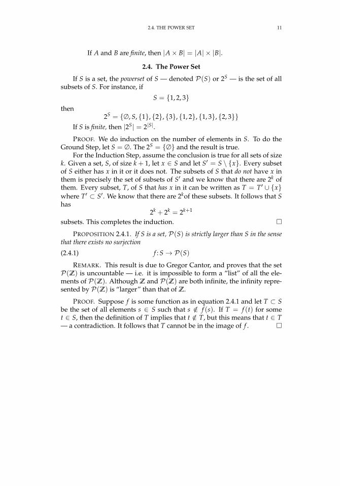
If S is a set, the powerset of S — denoted P(S) or 2S — is the set of allsubsets of S. For instance, if
S = 1, 2, 3then
2S = ∅, S, 1, 2, 3, 1, 2, 1, 3, 2, 3If S is finite, then |2S| = 2|S|.
PROOF. We do induction on the number of elements in S. To do theGround Step, let S = ∅. The 2S = ∅ and the result is true.
For the Induction Step, assume the conclusion is true for all sets of sizek. Given a set, S, of size k + 1, let x ∈ S and let S′ = S \ x. Every subsetof S either has x in it or it does not. The subsets of S that do not have x inthem is precisely the set of subsets of S′ and we know that there are 2k ofthem. Every subset, T, of S that has x in it can be written as T = T′ ∪ xwhere T′ ⊂ S′. We know that there are 2kof these subsets. It follows that Shas
2k + 2k = 2k+1
subsets. This completes the induction.
PROPOSITION 2.4.1. If S is a set, P(S) is strictly larger than S in the sensethat there exists no surjection
(2.4.1) f : S→ P(S)REMARK. This result is due to Gregor Cantor, and proves that the set
P(Z) is uncountable — i.e. it is impossible to form a “list” of all the ele-ments of P(Z). Although Z and P(Z) are both infinite, the infinity repre-sented by P(Z) is “larger” than that of Z.
PROOF. Suppose f is some function as in equation 2.4.1 and let T ⊂ Sbe the set of all elements s ∈ S such that s /∈ f (s). If T = f (t) for somet ∈ S, then the definition of T implies that t /∈ T, but this means that t ∈ T— a contradiction. It follows that T cannot be in the image of f .

CHAPTER 3
A glimpse of number theory
“Mathematics is the queen of the sciences and number theory isthe queen of mathematics. She often condescends to render ser-vice to astronomy and other natural sciences, but in all relationsshe is entitled to the first rank.”
— Carl Friedrich Gauss, in Gauss zum Gedächtniss (1856) byWolfgang Sartorius von Waltershausen.
3.1. Prime numbers and unique factorization
We begin by studying the algebraic properties of what would appear tobe the simplest and most basic objects possible: the integers. Study of theintegers is called number theory and some of the deepest and most difficultproblems in mathematics belong to this field.
Most people learned the following result in grade school — long divisionwith a quotient and remainder:
PROPOSITION 3.1.1. Let n and d be positive integers. Then it is possible towrite
n = q · d + rwhere 0 ≤ r < d. If r = 0, we say that d
∣∣ n — stated “d divides n”.
The division algorithm mentioned above gives rise to the concept ofgreatest common divisor.
DEFINITION 3.1.2. Let n and m be positive integers. The greatest com-mon divisor of n and m, denoted gcd(n, m), is the largest integer d such thatd∣∣ n and d
∣∣m. The least common multiple of n and m, denoted lcm(n, m), isthe smallest positive integer k such that n
∣∣ k and m∣∣ k.
Since 0 is divisible by any integer, gcd(n, 0) = gcd(0, n) = n.
There is a very fast algorithm for computing the greatest common di-visor due to Euclid — see [36, 37].
We need a lemma first:
LEMMA 3.1.3. If n > m > 0 are two integers and
n = q ·m + r
with 0 < r < m, thengcd(n, m) = gcd(m, r)
PROOF. If d∣∣ n and d
∣∣m, then d∣∣ r because
r = n− q ·m
13
14 3. A GLIMPSE OF NUMBER THEORY
On the other hand, if d∣∣m and d
∣∣ r, then
n = q ·m + r
implies that d∣∣ n. It follows that the common divisors of n and m are the
same as the common divisors of m and r. The same is true of the greatestcommon divisors.
ALGORITHM 3.1.4. Given positive integers n and m with n > m, use thedivision algorithm to set
n = q0 ·m + r0
m = q1 · r0 + r1
r0 = q2 · r1 + r2
...rk−2 = qk · rk−1 + rk
with m > r0 > r1 > · · · > rk. At some point rN = 0 and we claim thatrN−1 = gcd(n, m).
REMARK. Euclid’s original formulation was geometric, involving line-segments. Given two line-segments of lengths r1 and r2, it found a realnumber r such that
r1
r,
r2
r∈ Z
An ancient proof of the irrationality of√
2 showed that this processnever terminates if one of the line-segments is of unit length and the otheris the diagonal of a unit square.
PROOF. This follows from lemma 3.1.3 on the preceding page, appliedinductively.
As trivial as proposition 3.1.1 on the previous page appears to be, itallows us to prove Bézout’s Identity:
LEMMA 3.1.5. Let n and m be positive integers. Then there exist integers uand v such that
gcd(n, m) = u · n + v ·mREMARK. Bézout proved this identity for polynomials — see [13].
However, this statement for integers can be found in the earlier work ofClaude Gaspard Bachet de Méziriac (1581–1638) — see [103].
Étienne Bézout (1730–1783) was a French algebraist and geometer creditedwith the invention of the determinant (in [14]).
PROOF. Let z be the smallest positive value taken on by the expression
(3.1.1) z = u · n + v ·mas u and v run over all possible integers. Clearly, gcd(n, m)
∣∣ z sinceit divides any possible linear combination of m and n. It follows thatgcd(n, m) ≤ z.
3.1. PRIME NUMBERS AND UNIQUE FACTORIZATION 15
We claim that z∣∣ n. If not, then proposition 3.1.1 on page 13 implies
that n = q · z + r, where 0 < r < z, or r = n − q · z. Plugging that intoequation 3.1.1 on the preceding page gives
r = n− q · (u · n + v ·m)
= (1− q · u) · n− q · v ·mwhich is a linear combination of n and m smaller than z — a contradiction.Similar reasoning shows that z
∣∣m so z is a common divisor of m and n≥ gcd(m, n) so it must equal gcd(m, n).
DEFINITION 3.1.6. A prime number is an integer that is not divisible byany integer other than 1 or (±)itself.
Bézout’s Identity immediately implies:
PROPOSITION 3.1.7. Let p be a prime number and let n and m be integers.Then
p∣∣m · n =⇒ p
∣∣m or p∣∣ n
PROOF. Suppose p - m. We will show that p∣∣ n. Since p is prime and
p - m, we have gcd(p, m) = 1. Lemma 3.1.5 on the facing page implies thatthere exist integers u and v such that
1 = u ·m + v · pNow multiply this by n to get
n = u ·mn + v · n · pSince p divides each of the terms on the right, we get p
∣∣ n. A similar argu-ment show that p - n =⇒ p
∣∣m.
A simple induction shows that:
COROLLARY 3.1.8. If p is a prime number, ki ∈ Z for i = 1, . . . , n and
p∣∣ n
∏i=1
ki
then p|k j for at least one value of 1 ≤ j ≤ n. If p and q are both primes and
q∣∣ p
for some integer i ≥ 1, then p = q.
PROOF. We do induction on n. Proposition 3.1.7 proves the result forn = 2.
Suppose the result is known for n − 1 factors, and we have n factors.Write
n
∏i=1
ki = k1 ·(
n
∏i=2
ki
)Since
p∣∣ ki ·
(n
∏i=2
ki
)

16 3. A GLIMPSE OF NUMBER THEORY
we either have p|k or
p∣∣ n
∏i=2
ki
The inductive hypothesis proves the result. If the k j are all copies of aprime,p, we must have q
∣∣ p, which only happens if q = p.
This immediately implies the well-known result:
LEMMA 3.1.9. Let n be a positive integer and let
n = pα11 · · · · · p
αkk
= qβ11 · · · · · q
β``(3.1.2)
be factorizations into powers of distinct primes. Then k = ` and there is a reorder-ing of indices f : 1, . . . , k → 1, . . . , k such that qi = p f (i) and βi = α f (i) forall i from 1 to k.
PROOF. First of all, it is easy to see that a number can be factored intoa product of primes. We do induction on k. If k = 1 we have
pα11 = qβ1
1 · · · · · qβ``
Since q1|pα11 , corollary 3.1.8 on the preceding page implies that q1 = p1,
β1 = α1 and that the primes qi 6= p1 cannot exist in the product. So ` = 1and the conclusion follows.
Assume the result for numbers with k− 1 distinct prime factors. Equa-tion 3.1.2 implies that
q1∣∣ pα1
1 · · · · · pαkk
and corollary 3.1.8 on the preceding page implies that q1|∣∣ p for some value
of j. It also implies that pj = q1 and αj = β1. We define f (1) = j and take
the quotient of n by qβ11 = p
αjj to get a number with k − 1 distinct prime
factors. The inductive hypothesis implies the conclusion.
This allows us to prove the classic result:
COROLLARY 3.1.10 (Euclid). The number of prime numbers is infinite.
PROOF. Suppose there are only a finite number of prime numbers
S = p1, . . . , pnand form the number
K = 1 +n
∏i=1
pi
Lemma 3.1.9 implies that K can be uniquely factored into a product ofprimes
K = q1 · · · q`Since pi - K for all i = 1, . . . , n, we conclude that qj /∈ S for all j, so theoriginal set of primes, S, is incomplete.
Unique factorization also leads to many other results:
3.1. PRIME NUMBERS AND UNIQUE FACTORIZATION 17
PROPOSITION 3.1.11. Let n and m be positive integers with factorizations
n = pα11 · · · p
αkk
m = pβ11 · · · p
βkk
Then n|m if and only if αi ≤ βi for i = 1, . . . , k and
gcd(n, m) = pmin(α1,β1)1 · · · pmin(αk ,βk)
k
lcm(n, m) = pmax(α1,β1)1 · · · pmax(αk ,βk)
k
Consequently
(3.1.3) lcm(n, m) =nm
gcd(n, m)
PROOF. If n∣∣m, then pαi
i
∣∣ pβii for all i, by corollary 3.1.8 on page 15. If
k = gcd(n, m) with unique factorization
k = pγ11 · · · p
γkk
then γi ≤ αi and γi ≤ βi for all i. In addition, the γi must be as large as pos-sible and still satisfy these inequalities, which implies that γi = min(αi, βi)for all i. Similar reasoning implies statement involving lcm(n, m). Equa-tion 3.1.3 follows from the fact that
max(αi, βi) = αi + βi −min(αi, βi)
for all i.
The Extended Euclid algorithm explicitly calculates the factors that ap-pear in the Bézout Identity:
ALGORITHM 3.1.12. Suppose n, m are positive integers with n > n andwe use Euclid’s algorithm ( 3.1.4 on page 14) to compute gcd(n, m). Let qi, rifor 0 < i ≤ N (in the notation of 3.1.4 on page 14) denote the quotients andremainders used. Now define
x0 = 0y0 = 1(3.1.4)x1 = 1y1 = −q1
and recursively define
xk = xk−2 − qkxk−1
yk = yk−2 − qkyk−1(3.1.5)
for all 2 ≤ k ≤ N. Thenri = xi · n + yi ·m
so that, in particular,
gcd(n, m) = xN−1 · n + yN−1 ·m
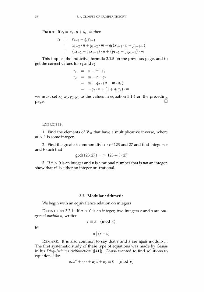
18 3. A GLIMPSE OF NUMBER THEORY
PROOF. If ri = xi · n + yi ·m then
rk = rk−2 − qkrk−1
= xk−2 · n + yk−2 ·m− qk(xk−1 · n + yk−1m)
= (xk−2 − qkxk−1) · n + (yk−2 − qkyk−1) ·mThis implies the inductive formula 3.1.5 on the previous page, and to
get the correct values for r1 and r2:
r1 = n−m · q1
r2 = m− r1 · q2
= m− q2 · (n−m · q1)
= −q2 · n + (1 + q1q2) ·mwe must set x0, x1, y0, y1 to the values in equation 3.1.4 on the precedingpage.
EXERCISES.
1. Find the elements of Zm that have a multiplicative inverse, wherem > 1 is some integer.
2. Find the greatest common divisor of 123 and 27 and find integers aand b such that
gcd(123, 27) = a · 123 + b · 27
3. If x > 0 is an integer and y is a rational number that is not an integer,show that xy is either an integer or irrational.
3.2. Modular arithmetic
We begin with an equivalence relation on integers
DEFINITION 3.2.1. If n > 0 is an integer, two integers r and s are con-gruent modulo n, written
r ≡ s (mod n)
ifn∣∣ (r− s)
REMARK. It is also common to say that r and s are equal modulo n.The first systematic study of these type of equations was made by Gaussin his Disquistiones Arithmeticae ([41]). Gauss wanted to find solutions toequations like
anxn + · · ·+ a1x + a0 ≡ 0 (mod p)

3.2. MODULAR ARITHMETIC 19
PROPOSITION 3.2.2. Equality modulo n respects addition and multiplica-tion, i.e. if r, s, u, v ∈ Z and n ∈ Z with n > 0, and
r ≡ s (mod n)
u ≡ v (mod n)(3.2.1)
then
r + u ≡ s + v (mod n)
r · u ≡ s · v (mod n)(3.2.2)
PROOF. The hypotheses imply the existence of integers k and ` suchthat
r− s = k · nu− v = ` · n
If we simply add these equations, we get
(r + u)− (s + v) = (k + `) · nwhich proves the first statement. To prove the second, note that
ru− sv = ru− rv + rv− sv
= r(u− v) + (r− s)v= r`n + kvn
= n(r`+ kv)
This elementary result has some immediate implications:
EXAMPLE. Show that 5|7k − 2k for all k ≥ 1. First note, that 7 ≡ 2(mod 5). Equation 3.2.2, applied inductively, implies that 7k ≡ 2k (mod 5)for all k > 1.
DEFINITION 3.2.3. If n is a positive integer, the set of equivalenceclasses of integers modulo n is denoted Zn.
REMARK. It is not hard to see that the size of Zn is n and the equiva-lence classes are represented by integers
0, 1, 2, . . . , n− 1Proposition 3.2.2 implies that addition and multiplication is well-definedin Zn. For instance, we could have an addition table for Z4 in table 3.2.1and a multiplication table in table 3.2.2 on the following page
+ 0 1 2 30 0 1 2 31 1 2 3 02 2 3 0 13 3 0 1 2
TABLE 3.2.1. Addition table for Z4
20 3. A GLIMPSE OF NUMBER THEORY
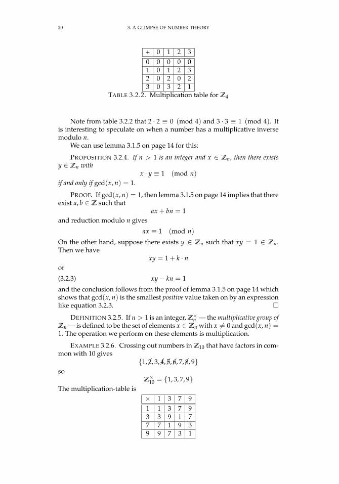
+ 0 1 2 30 0 0 0 01 0 1 2 32 0 2 0 23 0 3 2 1
TABLE 3.2.2. Multiplication table for Z4
Note from table 3.2.2 that 2 · 2 ≡ 0 (mod 4) and 3 · 3 ≡ 1 (mod 4). Itis interesting to speculate on when a number has a multiplicative inversemodulo n.
We can use lemma 3.1.5 on page 14 for this:
PROPOSITION 3.2.4. If n > 1 is an integer and x ∈ Zn, then there existsy ∈ Zn with
x · y ≡ 1 (mod n)if and only if gcd(x, n) = 1.
PROOF. If gcd(x, n) = 1, then lemma 3.1.5 on page 14 implies that thereexist a, b ∈ Z such that
ax + bn = 1and reduction modulo n gives
ax ≡ 1 (mod n)
On the other hand, suppose there exists y ∈ Zn such that xy = 1 ∈ Zn.Then we have
xy = 1 + k · nor
(3.2.3) xy− kn = 1
and the conclusion follows from the proof of lemma 3.1.5 on page 14 whichshows that gcd(x, n) is the smallest positive value taken on by an expressionlike equation 3.2.3.
DEFINITION 3.2.5. If n > 1 is an integer, Z×n — the multiplicative group ofZn — is defined to be the set of elements x ∈ Zn with x 6= 0 and gcd(x, n) =1. The operation we perform on these elements is multiplication.
EXAMPLE 3.2.6. Crossing out numbers in Z10 that have factors in com-mon with 10 gives
1, 2, 3, 4, 5, 6, 7, 8, 9so
Z×10 = 1, 3, 7, 9The multiplication-table is
× 1 3 7 91 1 3 7 93 3 9 1 77 7 1 9 39 9 7 3 1
3.3. THE EULER φ-FUNCTION 21
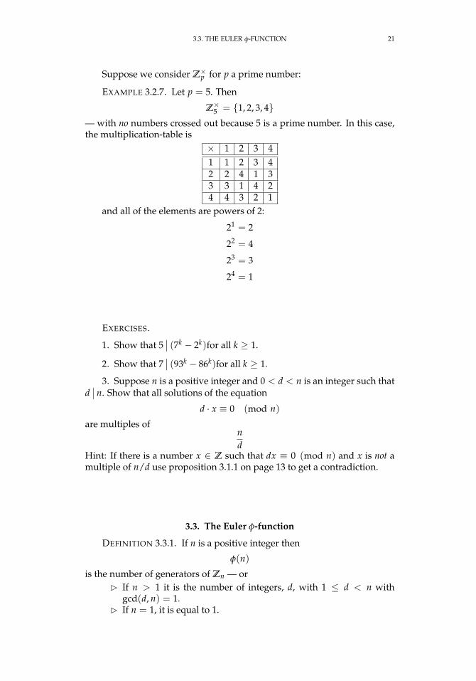
Suppose we consider Z×p for p a prime number:
EXAMPLE 3.2.7. Let p = 5. Then
Z×5 = 1, 2, 3, 4— with no numbers crossed out because 5 is a prime number. In this case,the multiplication-table is
× 1 2 3 41 1 2 3 42 2 4 1 33 3 1 4 24 4 3 2 1
and all of the elements are powers of 2:
21 = 2
22 = 4
23 = 3
24 = 1
EXERCISES.
1. Show that 5∣∣ (7k − 2k)for all k ≥ 1.
2. Show that 7∣∣ (93k − 86k)for all k ≥ 1.
3. Suppose n is a positive integer and 0 < d < n is an integer such thatd∣∣ n. Show that all solutions of the equation
d · x ≡ 0 (mod n)
are multiples ofnd
Hint: If there is a number x ∈ Z such that dx ≡ 0 (mod n) and x is not amultiple of n/d use proposition 3.1.1 on page 13 to get a contradiction.
3.3. The Euler φ-function
DEFINITION 3.3.1. If n is a positive integer then
φ(n)
is the number of generators of Zn — or If n > 1 it is the number of integers, d, with 1 ≤ d < n with
gcd(d, n) = 1. If n = 1, it is equal to 1.
22 3. A GLIMPSE OF NUMBER THEORY
This is called the Euler phi-function. Euler also called it the totient.
REMARK. Since an element x, of Zn has a multiplicative inverse if andonly if gcd(x, n) = 1 (see lemma 3.1.5 on page 14), it follows that the mul-tiplicative group Z×n has φ(n) elements, if n > 1.
This φ-function has some interesting applications
PROPOSITION 3.3.2. If n and m are integers > 1 with gcd(n, m) = 1, then
(3.3.1) mφ(n) ≡ 1 (mod n)
It follows that, for any integers a and b
(3.3.2) ma ≡ mb (mod n)
whenevera ≡ b (mod φ(n))
REMARK. Fermat proved this for n a prime number — in that case, itis called Fermat’s Little Theorem1.
Proposition 3.3.2 is a special case of a much more general result —corollary 4.4.3 on page 43.
PROOF. Let the elements of Z×n be
S = n1, . . . , nφ(n)where 1 ≤ ni < n for i = 1, . . . , φ(n). Since gcd(n, m) = 1, m is one ofthem. Now multiply all of these integers by m and reduce modulo n (so theresults are between 1 and n− 1). We get
T = mn1, . . . , mnφ(n)These products are all distinct because m has a multiplicative inverse, so
mni ≡ mnj (mod n)
implies
m−1mni ≡ m−1mnj (mod n)
ni ≡ nj (mod n)
The Pigeonhole Principle implies that as sets
Z×n = n1, . . . , nφ(n) = mn1, . . . , mnφ(n)— in other words, the list T is merely a permutation of S. Now we multiplyeverything in S and T together
n1 · · · nφ(n) ≡ b (mod n)
mn1 · · ·mnφ(n) ≡ mφ(n)b (mod n)
≡ b (mod n) since Tis a permutation of S
Multiplication by b−1 proves equation 3.3.1.
1Fermat’s Big Theorem is the statement that an + bn = cn has no positive integer solutionsfor n an integer > 2. This was only proved in 1993 by Andrew Wiles.
3.3. THE EULER φ-FUNCTION 23
EXAMPLE. What is the low-order digit of 71000? This is clearly 71000
modulo 10. Example 3.2.6 on page 20 shows that φ(10) = 4. Since 4|1000,equation 3.3.2 on the facing page implies that
71000 ≡ 70 ≡ 1 (mod 10)
so the answer to the question is 1.
If p is a prime number, every integer between 1 and p− 1 is relativelyprime to p, so φ(p) = p− 1 (see example 3.2.7 on page 21). In fact, it is nothard to see that
PROPOSITION 3.3.3. If p is a prime number and k ≥ 1 is an integer, then
φ(pk) = pk − pk−1
PROOF. The only integers 0 ≤ x < p − 1 that have the property thatgcd(x, pk) 6= 1 are multiples of p — and there are pk−1 = pk/p of them.
It turns out to be fairly easy to compute φ(n) for all n. To do this, weneed the Chinese Remainder Theorem:
LEMMA 3.3.4. If n and m are positive integers with gcd(n, m) = 1 and
x ≡ a (mod n)
x ≡ b (mod m)(3.3.3)
are two congruences, then they have a unique solution modulo nm.
PROOF. We explicitly construct x. Since gcd(n, m) = 1 , there existintegers u and v such that
(3.3.4) u · n + v ·m = 1
Now define
(3.3.5) x = b · u · n + a · v ·m (mod nm)
Equation 3.3.4 implies that
vm ≡ 1 (mod n) so x ≡ a (mod n) un ≡ 1 (mod m) so x ≡ b (mod m).
Suppose x′ is another value modulo nm satisfying equation 3.3.3. Then
x′ − x ≡ 0 (mod n)
x′ − x ≡ 0 (mod m)(3.3.6)
which implies that x′ − x is a multiple of both n and m. The conclusion fol-lows from equation 3.1.3 on page 17, which shows that x′ − x is a multipleof nm, so x′ ≡ x (mod nm).
Using this, we can derive the full theorem
24 3. A GLIMPSE OF NUMBER THEORY
THEOREM 3.3.5 (Chinese Remainder Theorem). If n1, . . . , nk are a set ofpositive integers with gcd(ni, nj) = 1 for all 1 ≤ i < j ≤ k, then the equations
x ≡ a1 (mod n1)
...
x ≡ ak (mod nk)
have a unique solution modulo ∏ki=1 ni.
REMARK. The Chinese Remainder Theorem was first published some-time between the 3rd and 5th centuries by the Chinese mathematician SunTzu (not to be confused with the author of “The Art of Warfare”).
PROOF. We do induction on k. Lemma 3.3.4 proves it for k = 2. Weassume it is true for k = j− 1 — which means we have equations
x ≡ b (mod n1 · · · nj−1)
x ≡ aj (mod nj)
where b is whatever value the theorem provided for the first j − 1 equa-tions.
Note that the hypotheses imply that the sets of primes occurring in thefactorizations of the ni are all disjoint. It follows that the primes in the fac-torization of n1 · · · nj−1 will be disjoint from the primes in the factorizationof nj. It follows that
gcd(n1 · · · nj−1, nj) = 1and the conclusion follows from an additional application of lemma 3.3.4.
COROLLARY 3.3.6. If n and m are integers > 1 such that gcd(n, m) = 1,then
φ(nm) = φ(n)φ(m)
PROOF. The correspondence in the Chinese Remainder Theorem(lemma 3.3.4 on the previous page) actually respects products: If
x ≡ a (mod n)
x ≡ b (mod m)(3.3.7)
and
y ≡ a−1 (mod n)
y ≡ b−1 (mod m)(3.3.8)
thenxy ≡ 1 (mod nm)
since the value is unique modulo nm and reduces to 1 modulo n and m. Itfollows that there is a 1-1 correspondence between pairs, (a, b) with a ∈ Z×n ,b ∈ Z×m and elements of Z×nm — i.e., as sets,
Z×nm = Z×n ×Z×mproving the conclusion.
3.4. APPLICATIONS TO CRYPTOGRAPHY 25
At this point, computing φ(n) for any n becomes fairly straightforward.If
n = pk11 · · · p
ktt
then
φ(n) =(
pk11 − pk1−1
1
)· · ·(
pktt − pkt−1
t
)(3.3.9)
= pk1−11 (p1 − 1) · · · pkt−1
t (pt − 1)
EXERCISES.
1. Compute φ(52).
2. Compute the low-order two digits of 71000.
3.4. Applications to cryptography
In this section, we will describe a cryptographic system that everyonereading this book has used — probably without being aware of it.
A regular cryptographic system is like a locked box with a key — andone cannot open the box without the key. The cryptographic system wediscuss here is like a magic box with two keys — if one key is used to lock thebox only the other key can open it. It is called a public-key system and wasfirst publicly described by Ron Rivest, Adi Shamir and Leonard Adlemanin 1977.
One application of this system is to make one of the keys public — soanyone who wants to communicate with you can use it to encrypt the mes-sage. Your evil enemies (!) cannot read the message because the other key(the one you keep private) is the only one that can decrypt it.
Another application involves digital signatures:How do you sign a document (like an email) in the digitalage?
Typing your name at the bottom is clearly inadequate — anyone can typeyour name. Even an ink signature on a paper document is highly flawedsince robotic signing machines can mimic a person’s handwriting perfectly.
The answer: encrypt the document with your private key. In this case,the goal is not to hide the message. If your public key can decrypt it, themessage must have come from you.
So here is the RSA system, the first public key system ever devised (andthe one most widely used to this day):
We start with two large primes (large=50 digits or so), p and q, andintegers m and n that satisfy
gcd(n, φ(pq)) = 1
n ·m ≡ 1 (mod φ(pq))
26 3. A GLIMPSE OF NUMBER THEORY
Proposition 3.3.2 implies that
xnm ≡ x (mod pq)
whenever gcd(x, pq) = 1.Our public key is the pair (pq, n) and the encryption of a number k in-
volvesk 7→ e = kn (mod pq)
where e is the encrypted message. The private key is m and decryption in-volves
e = kn 7→ em = knm ≡ k (mod pq)One may wonder how secure this system is. We know that
φ(pq) = (p− 1)(q− 1)
(from proposition 3.3.3 on page 23 and lemma 3.3.4 on page 23), so if yourevil enemies know (p− 1)(q− 1), they can easily2 compute m, given n. Theproblem boils down to computing (p− 1)(q− 1) when one only knows pq.
Oddly enough, this can be very hard to do. The only known way offinding (p− 1)(q− 1) from pq involves factoring pq into p and q.
Recall how we factor numbers: try primes like 2, 3, 5, . . . until we findone that divides the number. If the smallest prime that divides pq is 50 digitslong, even a computer will have major problems factoring it.
Now we return to the statement made at the beginning of the section:every reader has used this system. That is because secure web transactions useit: A web server sends its public key to your web browser which encryptsyour credit-card number (for instance) and sends it back to the server.
EXERCISES.
1. Suppose p = 11 and q = 13. Compute public and private keys foran RSA cryptosystem using these.
3.5. Quadratic Residues
If p is a prime, consider the multiplicative group Z×p — see definition 3.2.5 onpage 20. If we write X2 = 1 or X2 − 1 = 0, we can factor it as
(X− 1)(X + 1) = 0
which implies that the only elements of Z×p that are their own inverses are ±1. Itfollows that in the list
2, 3, . . . , p− 3, p− 2
2OK, maybe not easily, but there are well-known methods for this, using Algorithm 3.1.12on page 17.

3.5. QUADRATIC RESIDUES 27
every element will be paired with its multiplicative inverse. This implies that
(p− 2)! ≡ 1 (mod p)
and(p− 1)! ≡ p− 1 ≡ −1 (mod p)
or(p− 1)! + 1 ≡ 0 (mod p)
This leads into
THEOREM 3.5.1 (Wilson’s Theorem). If n > 1 is an integer, then n is a prime if andonly if
(3.5.1) (n− 1)! + 1 ≡ 0 (mod n)
REMARK. In principle, this could be used as a test for primality. In practice,computing (n− 1)! is too computationally expensive.
This theorem was stated by Ibn al-Haytham (c. 1000 AD), and, in the 18thcentury, by John Wilson. In [105], Edward Waring announced the theorem in 1770,although neither he nor his student Wilson could prove it. Lagrange gave the firstproof in 1771 (see [67]). There is evidence that Leibniz was also aware of the resulta century earlier, but he never published it.
PROOF. We have already proved it in the case where n is a prime. If n = k`with k, ` > 1 then
(n− 1)! + 1 ≡ 0 (mod n)implies that
(n− 1)! + 1 ≡ 0 (mod k)which is a contradiction since k occurs as a factor in (n− 1)! so that
(n− 1)! ≡ 0 (mod k)
The reasoning in Wilson’s Theorem allows us to explore the question of qua-dratic residues — squares of elements modulo a prime.
DEFINITION 3.5.2. Let p be a prime number and let n > 0 be an integer. Definethe Legendre symbol(
np
)=
1 if p - n and ∃x with n ≡ x2 (mod p)−1 if p - n and @x with n ≡ x2 (mod p)0 if p
∣∣ n
REMARK. Legendre symbols are used to solve quadratic equations in Zp.
We can get a useful computational formulation of the Legendre symbol
THEOREM 3.5.3 (Euler’s Criterion). If p is an odd prime number and n > 0 is aninteger, then (
np
)≡ n
p−12 (mod p)
PROOF. Clearly true if p∣∣ n. If n ≡ x2 (mod p) then
np−1
2 ≡ xp−1 ≡ 1 (mod p)
by proposition 3.3.2 on page 22. If n is not the square of any element of Z×p , definetwo elements x, y ∈ 1, . . . , p− 1 to be associates if
x · y ≡ n (mod p)

28 3. A GLIMPSE OF NUMBER THEORY
Every element of 1, . . . , p − 1 has a unique associate distinct from itself. If m =(p− 1)/2, the list
x1, y1, x2, y2, . . . , xm, ymwhere xi is associated to yi, is just a permutation of the list
1, . . . , p− 1so that
x1 · y1 · x2 · y2 · · · xm · ym ≡ nm (mod p)
≡ 1 · 2 · 3 · · · (p− 1) ≡ −1 (mod p)
by theorem 3.5.1 on the previous page. The conclusion follows.
This immediately implies
COROLLARY 3.5.4. If p > 1 is a prime and n, m > 0 are integers, then(np
)(mp
)=
(nmp
)REMARK. This facilitates computation of Legendre symbols: if
n = pα11 · · · p
αkk
is the prime factorization of n and i1, . . . , it are the subscripts for which the corre-sponding exponents αij are odd, then(
np
)=
(pi1
p
)· · ·(
pit
p
)so the computation of
(np
)is reduced to computing
(qp
)for prime values of q.
One of the most important tools for computing these is
THEOREM 3.5.5 (Law of Quadratic Reciprocity). If p and q are distinct odd primes,then (
pq
)(qp
)= (−1)
p−12 ·
q−12
REMARK. This beautiful theorem was conjectured by Euler and Legendre andfirst proved by Gauss in 1796 in [41]. He called it his “golden theorem,” and pub-lished six proofs of it in his lifetime. Two more were found in his posthumouspapers.
There are now over 240 published proofs of this result.
PROOF. The proof given here is due to George Rousseau — see [95].The Chinese Remainder Theorem (see lemma 3.3.4 on page 23) implies that the
map
τ: Z×pq →Z×p ×Z×qn 7→(n mod p, n mod q)
is a bijection that preserves products, where multiplication in Z×p ×Z×q is definedby (a, b) · (c, d) = (a · c, b · d). Define
L =
k ∈ Z×pq|1 ≤ k <pq2
and
R =(a, b) ∈ Z×p ×Z×q |1 ≤ b <
q2
They are chosen so for all x ∈ Z×pq either x or −x ∈ L but not both, and for any(a, b) ∈ Z×p ×Z×q either (a, b) ∈ R or −(a, b) ∈ R but not both. For any (a, b) ∈ R,
3.5. QUADRATIC RESIDUES 29
there exists a unique k ∈ Z×pq such that τ(k) = (a, b), and either k or −k is in L. Wehave
(3.5.2) ∏(a,b)∈R
(a, b) = ε ∏k∈L
(k mod p, k mod q)
where ε = ±1.Set P = (p− 1)/2 and Q = (q− 1)/2. Then we can evaluate the left side of
equation 3.5.2 via
∏(a,b)∈R
(a, b) = ∏a<p
b<q/2
(a, b) =((p− 1)!Q, Q!2P
)
=
((−1)Q,
((q− 1)!(−1)Q
)P)
=((−1)Q, (−1)P(−1)PQ
)The middle step follows from the fact that(
1 · · · q− 12
)2= 1 · · · q− 1
2· 1 · · · q− 1
2
= 1 · · · q− 12· (− q− 1
2) · · · (−1) · (−1)Q (mod q)
= (q− 1)!(−1)Q
since q−(
q−12 − k
)≡ −
(q+1
2 + k)
(mod q) for k = 0, . . . , q−12 − 1.
Now we analyze the right side of equation 3.5.2. We start with the left factor:
∏k∈L
k mod p = ∏k<pq/2
gcd(k,pq)=1
k mod p
=
(∏
k<pq/2p-k
k mod p)(
∏k<pq/2
q∣∣ k
k mod p)−1
=
Q−1
∏j=0
(∏
jp<k<(j+1)pk mod p
)( ∏Qp<k<pq/2
k mod p)
·(
∏k<pq/2
q∣∣ k
k mod p)−1
=(p− 1)!QP!
(q)(2q) · · · (Pq)=
(−1)Q
qP
= (−1)Q(
qp
)(see Euler’s Criterion, theorem 3.5.3)
By symmetry, the right factor must satisfy
∏k∈L
k mod q = (−1)P(
pq
)so that equation 3.5.2 becomes(
(−1)Q, (−1)P(−1)PQ)= ε
((−1)Q
(qp
), (−1)P
(pq
))
30 3. A GLIMPSE OF NUMBER THEORY
Equating the left factors shows that
ε =
(qp
)and equating the right factors implies that
(−1)PQ =
(qp
)(pq
)which is the theorem’s statement.
Now we can compute!
EXAMPLE 3.5.6. Is 11 a square modulo 53? We must compute(
1153
). Quadratic
Reciprocity show that (1153
)(5311
)= (−1)5·26 = 1
but (5311
)=
(53 mod 11
11
)=
(9
11
)=
(3
11
)2= 1
so we conclude that 11 is a square modulo 53.
One possible difficulty might involve computing(2p
)In this case, we use the fact that Legendre symbols only depend on the equivalenceclass modulo p so that(
2p
)=
(2− p
p
)=
(−1p
)(p− 2
p
)= (−1)
p−12
(p− 2
p
)EXAMPLE 3.5.7. Compute (
102113
)Since 102 = 2 · 3 · 17, we have(
102113
)=
(2
113
)·(
3113
)·(
17113
)Now
(2
113
)= (−1)56
(111113
)=(
3113
) (37
113
), so
(102113
)=(
3113
)2·(
17113
)·(
37113
)=(
17113
)·(
37113
). Now we use Quadratic Reciprocity to conclude that(
17113
)(11317
)= (−1)8·56 = 1
and(
11317
)=(
1117
)and Quadratic Reciprocity implies that(
1117
)(1711
)= (−1)5·8 = 1
But(
1711
)=(
611
)=(
211
)·(
311
). We conclude that
(211
)= −
(9
11
)= −1. The
factor (311
)(113
)= (−1)1·5 = −1
We get(
113
)=(
23
)= −1 (by direct computation), so
(311
)=(
1711
)=(
1117
)=(
11317
)=(
17113
)= −1.
3.5. QUADRATIC RESIDUES 31
The factor(
37113
)satisfies(
37113
)(11337
)= (−1)18·56 = 1
and(
11337
)=(
237
)= (−1)18
(3537
)=(
537
) (737
). For the first factor(
537
)(375
)= (−1)2·18 = 1
and(
375
)=(
25
)= −1 (by direct computation). For the second factor(
737
)(377
)= (−1)3·18 = 1
and(
377
)=(
27
)= 1, since 32 ≡ 2 (mod 7).
We finally conclude that(
11337
)=(
37113
)= −1 and(
102113
)= (−1)(−1) = 1
so that 102 is a square modulo 113.

CHAPTER 4
Group Theory
“The introduction of the digit 0 or the group concept was gen-eral nonsense too, and mathematics was more or less stagnatingfor thousands of years because nobody was around to take suchchildish steps. . . ”
— Alexander Grothendieck, writing to Ronald Brown.
4.1. Introduction
One of the simplest abstract algebraic structures is that of the group. Inhistorical terms its development is relatively recent, dating from the early1800’s. The official definition of a group is due to Évariste Galois, used indeveloping Galois Theory (see chapter 8 on page 295).
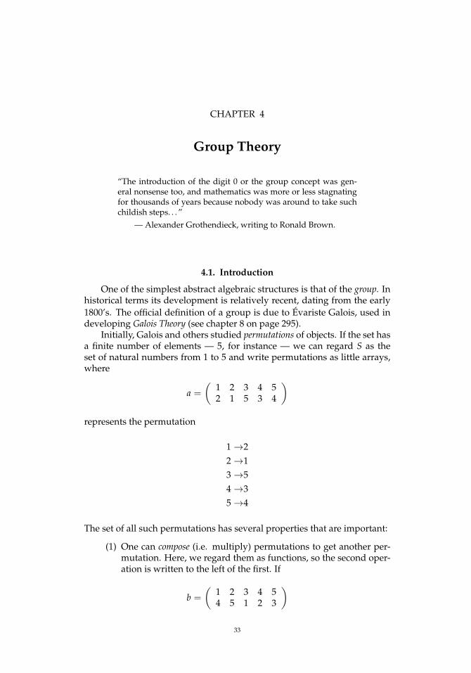
Initially, Galois and others studied permutations of objects. If the set hasa finite number of elements — 5, for instance — we can regard S as theset of natural numbers from 1 to 5 and write permutations as little arrays,where
a =
(1 2 3 4 52 1 5 3 4
)represents the permutation
1→22→13→54→35→4
The set of all such permutations has several properties that are important:
(1) One can compose (i.e. multiply) permutations to get another per-mutation. Here, we regard them as functions, so the second oper-ation is written to the left of the first. If
b =
(1 2 3 4 54 5 1 2 3
)
33
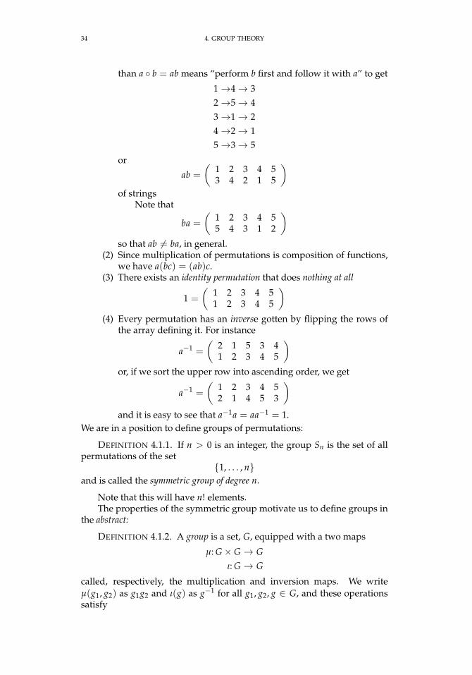
34 4. GROUP THEORY
than a b = ab means “perform b first and follow it with a” to get
1→4→ 32→5→ 43→1→ 24→2→ 15→3→ 5
or
ab =
(1 2 3 4 53 4 2 1 5
)of strings
Note that
ba =
(1 2 3 4 55 4 3 1 2
)so that ab 6= ba, in general.
(2) Since multiplication of permutations is composition of functions,we have a(bc) = (ab)c.
(3) There exists an identity permutation that does nothing at all
1 =
(1 2 3 4 51 2 3 4 5
)(4) Every permutation has an inverse gotten by flipping the rows of
the array defining it. For instance
a−1 =
(2 1 5 3 41 2 3 4 5
)or, if we sort the upper row into ascending order, we get
a−1 =
(1 2 3 4 52 1 4 5 3
)and it is easy to see that a−1a = aa−1 = 1.
We are in a position to define groups of permutations:
DEFINITION 4.1.1. If n > 0 is an integer, the group Sn is the set of allpermutations of the set
1, . . . , nand is called the symmetric group of degree n.
Note that this will have n! elements.The properties of the symmetric group motivate us to define groups in
the abstract:
DEFINITION 4.1.2. A group is a set, G, equipped with a two maps
µ: G× G → Gι: G → G
called, respectively, the multiplication and inversion maps. We writeµ(g1, g2) as g1g2 and ι(g) as g−1 for all g1, g2, g ∈ G, and these operationssatisfy
4.1. INTRODUCTION 35
(1) there exists an element 1 ∈ G such that 1g = g1 = g for all g ∈ G(2) for all g ∈ G, gg−1 = g−1g = 1(3) for all g1, g2, g3 ∈ G, g1(g2g3) = (g1g2)g3
If the group G is finite, the number of elements of G is denoted |G| andcalled the order of G. If for any elements a, b ∈ G, ab = ba, we say that G isabelian.
REMARK. Rather confusingly, the group-operation for an abeliangroup is often written as addition rather than multiplication.
In the beginning all groups were groups of permutations, many ofwhich were used for geometric purposes.
We have already seen a few examples of groups:
EXAMPLE 4.1.3. for any positive integer, Zn is a group under the oper-ation of addition. We can indicate this by writing it as (Zn,+).
We can take a similar set of numbers and give it a group-structure in adifferent way:
EXAMPLE 4.1.4. Z×n is a group under the operation ofinteger-multiplication1, or (Z×n ,×) — although multiplication is generallyimplied by the ×-superscript.
Here are some others:
EXAMPLE 4.1.5. The set of real numbers, R, forms a group under addi-tion: (R,+).
We can do to R something similar to what we did with Zn in exam-ple 4.1.4:
EXAMPLE 4.1.6. The set of nonzero reals, R× = R \ 0, forms agroup under multiplication, Again, the group-operation is implied by the×-superscript.
We can roll the real numbers up into a circle and make that a group:
EXAMPLE 4.1.7. S1 ⊂ C — the complex unit circle, where the group-operation is multiplication of complex numbers.
Let us consider a group defined geometrically. Consider the unit squarein the plane in figure 4.1.1 on the following page. If we consider all pos-sible rigid motions of the plane that leave it fixed, we can represent theseby the induced permutations of the vertices. For instance the 90 coun-
terclockwise rotation is represented by R =
(1 2 3 42 3 4 1
). Composing
this with itself gives
R2 =
(1 2 3 43 4 1 2
)and
R3 =
(1 2 3 44 1 2 3
)
36 4. GROUP THEORY
1 2
34
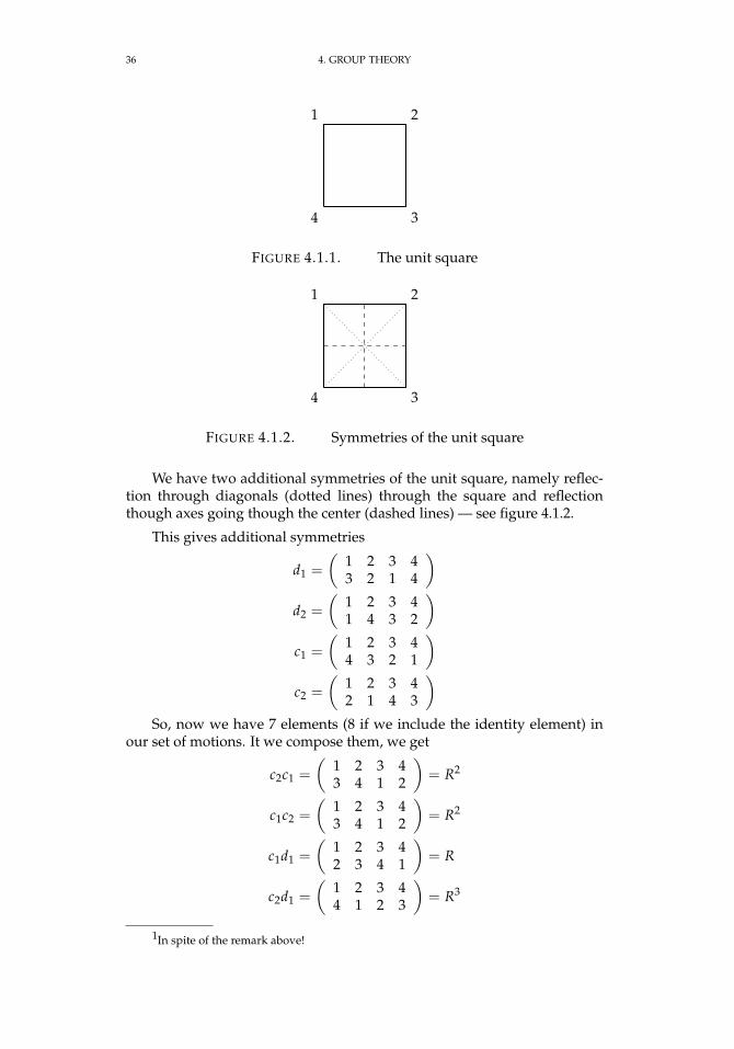
FIGURE 4.1.1. The unit square
1 2
34
FIGURE 4.1.2. Symmetries of the unit square
We have two additional symmetries of the unit square, namely reflec-tion through diagonals (dotted lines) through the square and reflectionthough axes going though the center (dashed lines) — see figure 4.1.2.
This gives additional symmetries
d1 =
(1 2 3 43 2 1 4
)d2 =
(1 2 3 41 4 3 2
)c1 =
(1 2 3 44 3 2 1
)c2 =
(1 2 3 42 1 4 3
)So, now we have 7 elements (8 if we include the identity element) in
our set of motions. It we compose them, we get
c2c1 =
(1 2 3 43 4 1 2
)= R2
c1c2 =
(1 2 3 43 4 1 2
)= R2
c1d1 =
(1 2 3 42 3 4 1
)= R
c2d1 =
(1 2 3 44 1 2 3
)= R3
1In spite of the remark above!
4.1. INTRODUCTION 37
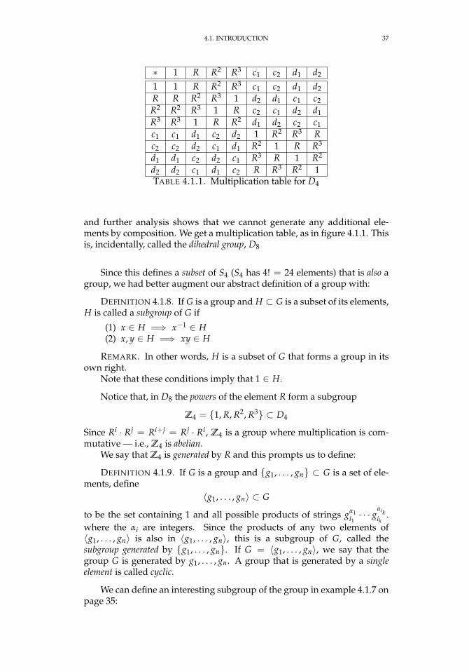
∗ 1 R R2 R3 c1 c2 d1 d2
1 1 R R2 R3 c1 c2 d1 d2R R R2 R3 1 d2 d1 c1 c2R2 R2 R3 1 R c2 c1 d2 d1R3 R3 1 R R2 d1 d2 c2 c1c1 c1 d1 c2 d2 1 R2 R3 Rc2 c2 d2 c1 d1 R2 1 R R3
d1 d1 c2 d2 c1 R3 R 1 R2
d2 d2 c1 d1 c2 R R3 R2 1TABLE 4.1.1. Multiplication table for D4
and further analysis shows that we cannot generate any additional ele-ments by composition. We get a multiplication table, as in figure 4.1.1. Thisis, incidentally, called the dihedral group, D8
Since this defines a subset of S4 (S4 has 4! = 24 elements) that is also agroup, we had better augment our abstract definition of a group with:
DEFINITION 4.1.8. If G is a group and H ⊂ G is a subset of its elements,H is called a subgroup of G if
(1) x ∈ H =⇒ x−1 ∈ H(2) x, y ∈ H =⇒ xy ∈ H
REMARK. In other words, H is a subset of G that forms a group in itsown right.
Note that these conditions imply that 1 ∈ H.
Notice that, in D8 the powers of the element R form a subgroup
Z4 = 1, R, R2, R3 ⊂ D4
Since Ri · Rj = Ri+j = Rj · Ri, Z4 is a group where multiplication is com-mutative — i.e., Z4 is abelian.
We say that Z4 is generated by R and this prompts us to define:
DEFINITION 4.1.9. If G is a group and g1, . . . , gn ⊂ G is a set of ele-ments, define
〈g1, . . . , gn〉 ⊂ G
to be the set containing 1 and all possible products of strings gα1i1· · · gαik
ik.
where the αi are integers. Since the products of any two elements of〈g1, . . . , gn〉 is also in 〈g1, . . . , gn〉, this is a subgroup of G, called thesubgroup generated by g1, . . . , gn. If G = 〈g1, . . . , gn〉, we say that thegroup G is generated by g1, . . . , gn. A group that is generated by a singleelement is called cyclic.
We can define an interesting subgroup of the group in example 4.1.7 onpage 35:
38 4. GROUP THEORY
EXAMPLE 4.1.10. If p is a prime, define Z/p∞ to be the multiplicativesubgroup of the unit circle in C generated by elements of the form e2πi/pk
for all integers k > 0. This is called a Prüfer group.
Every element of a group generates a cyclic subgroup:
DEFINITION 4.1.11. If G is a group and g ∈ G is an element, the set ofall powers of g forms a subgroup of G denoted 〈g〉 ⊂ G. If G is finite, theorder of this subgroup is called the order of g, denoted ord(g).
When we have two groups, G and H, we can build a new group fromthem:
DEFINITION 4.1.12. If G and H are groups, their direct sum, G ⊕ H, isthe set of all possible pairs (g, h) with g ∈ G, h ∈ H and group-operation
(g1, h1)(g2, h2) = (g1g2, h1h2)
The groupK = Z2 ⊕Z2
is called the Klein 4-group.
EXERCISES.
1. If G is a group and 11 and 12 are two identity elements, show that
11 = 12
so that a group’s identity element is unique.
2. If G is a group and a, b, c ∈ G show that ab = ac implies that b = c.
3. Find elements a, b ∈ D4 such that (ab)−1 6= a−1b−1.
4. If G is a group and a, b ∈ G have the property that ab = 1, show thatba = 1.
5. If G is a group and a, b ∈ G, show that (ab)−1 = b−1a−1 — so wemust reverse the order of elements in a product when taking an inverse.
6. List all of the generators of the cyclic group, Z10.
7. Show that the set
±3k|k ∈ Z ⊂ R×
is a subgroup.
8. Show that the set(1 2 31 2 3
),(
1 2 31 3 2
)is a subgroup of S3.
9. Show that D4 = 〈R, d1〉.
4.2. HOMOMORPHISMS 39
10. If G = Z×p for a prime number p, define
G2 =
x2∣∣∣∣x ∈ G
Show that G2 ⊂ G is a subgroup of order (p− 1)/2 if p is odd, and order 1if p = 2.
11. If g ∈ G is an element of a finite group, show that there exists aninteger n > 0 such that gn = 1.
12. Prove that the operation x ∗ y = x + y + xy on the set x ∈ R,x 6= −1, defines an abelian group.
13. List all of the subgroups of a Klein 4-group.
4.2. Homomorphisms
Now we consider functions from one group to another, and the ques-tion of when two groups are mathematically equivalent (even when theyare defined in very different ways).
We start with a pointlessly abstract definition of a function:
DEFINITION 4.2.1. If S and T are sets, a function
f : S→ T
is a set of pairsf ⊂ S× T
– i.e., (s1, t1), . . . , (sj, tj) with the property that(1) every element of S occurs as the first member of some pair(2) for any two pairs (s1, t1) and (s2, t2), s1 = s2 implies that t1 = t2.
If (s, t) ∈ f ⊂ S× T, we write f (s) = t. The set S is called the domain of fand T is called the range. The set of t ∈ T such f (s) = t for some s ∈ S iscalled the image or codomain of f .
REMARK. In other words, f just associates a unique element of T toevery element of S.
For instance, f (x) = x2 defines a function whose domain and range isR. The equation f (x) =
√x defines a function whose domain and range
are R+ — real numbers ≥ 0.Having defined functions, we also distinguish various types of func-
tions:
DEFINITION 4.2.2. A function, f : S → T, is injective if f (s1) = f (s2)implies s1 = s2. It is surjective if for every t ∈ T, there exists an s ∈ S suchthat f (s) = t — so the image of f is all of T. It is bijective if it is injective andsurjective.
The reader may wonder what all of this has to do with groups.
40 4. GROUP THEORY
DEFINITION 4.2.3. If G and H are groups and
f : G → H
is a function, f is called a homomorphism if it preserves group-operations,i.e. for all g1, g2 ∈ G
f (g1g2) = f (g1) f (g2) ∈ H
The set of all elements g ∈ G such that f (g) = 1 ∈ H is called the kernel off , denoted ker f . If f is bijective, it is called an isomorphism and the groupsG and H are said to be isomorphic. An isomorphism from a group to itselfis called an automorphism.
A homomorphism f : G → H has certain elementary properties that weleave as exercises to the reader:
EXERCISES.
1. Show that f (1) = 1 ∈ H
2. Show that f (g−1) = f (g)−1
3. Show that ker f ⊂ G is a subgroup
4. Show that im f ⊂ H is a subgroup
5. If S1 is the complex unit circle (see example 4.1.7 on page 35), showthat the function
f : R→ S1
mapping x ∈ R to eix ∈ S1 is a homomorphism. What is its kernel?
6. Show that the map
f : Z → Zn
i 7→ i (mod n)
is a homomorphism.
7. If m and n are positive integers with gcd(m, n) = 1, show that
Zm ⊕Zn ∼= Zmn
Z×m ⊕Z×n ∼= Z×mn
4.3. Cyclic groups
Cyclic groups are particularly easy to understand since they only havea single generator. In fact, we have already studied such groups because:
PROPOSITION 4.3.1. Let G be a cyclic group(1) If |G| = n, then G is isomorphic to Zn.
4.3. CYCLIC GROUPS 41
(2) If |G| = ∞, then G is isomorphic to Z.
REMARK. When |G| ∼= Z, it is called an infinite cyclic group.
PROOF. Since G is cyclic it consists of powers of a single element G
1, g, . . . , gk, . . . and the isomorphism maps gk to k in Zn or Z, respectively.
PROPOSITION 4.3.2. If G is a cyclic group and H ⊂ G is a subgroup, thenH is cyclic.
PROOF. Suppose G is generated by an element g andH = 1, gn1 , gn2 , . . . . If α = min|n1|, . . . , we claim that gα generates H.If not, there exists a gn ∈ H such that α - n. In this case
n = α · q + r
with 0 < r < α and gr = gn · (gα)−q ∈ H with r < α. This is a contradiction.
EXERCISE 4.3.3. If n and d are a positive integers such that d∣∣ n, show
that there exists a unique subgroup, S ⊂ Zn, with d elements Hint: propo-sition 4.3.2 implies that S is cyclic, so every element is a multiple of a gener-ator g ∈ S with d · g ≡ 0 (mod d) If x = k · g ∈ S, this means that d · x ≡ 0(mod n). Now look at exercise 3 on page 21.
If G = Zn, and d∣∣ n, then the set
(4.3.1)
0,nd
, 2nd
, . . . , (d− 1)nd
forms this unique subgroup isomorphic to Zd.
REMARK. In Zn, the group-operation is written additively, so the orderof m ∈ Zn (see definition 4.1.11 on page 38) 4.1.11 on page 38is the smallestk > 0 such that
k ·m ≡ 0 (mod n)
PROPOSITION 4.3.4. If m ∈ Zn is a nonzero element, then
ord(m) =n
gcd(n, m)
It follows that m 6= 0 is a generator of Zn if and only if gcd(n, m) = 1.
REMARK. It follows that Zn has precisely φ(n) distinct generators.
PROOF. The order of m is the smallest k such that k ·m = 0 ∈ Zn, i.e.,
k ·m = ` · nfor some integer `. It follows that k · m is the least common multiple of mand n. Since
lcm(n, m) =nm
gcd(n, m)
— see proposition 3.1.11 on page 17, we getnm
gcd(n, m)= k ·m
42 4. GROUP THEORY
andk =
ngcd(n, m)
The number m is a generator of Zn if and only if ord(m) = n — be-cause it has n distinct multiples in this case — which happens if and only ifgcd(n, m) = 1.
As basic as this result is, it implies something interesting about the Eu-ler φ-function:
LEMMA 4.3.5. If n is a positive integer, then
(4.3.2) n = ∑d|n
φ(d)
where the sum is taken over all positive divisors, d, of n.
PROOF. If d∣∣ n, let Φd ⊂ Zn be the set of generators of the unique
cyclic subgroup of order d (generated by n/d). Since every element of Zngenerates one of the Zd, it follows that Zn is the disjoint union of all of theΦd for all divisors d
∣∣ n. This implies that
|Zn| = n = ∑d|n|Φd| = ∑
d|nφ(d)
For instance
φ(20) = φ(4) · φ(5)= (22 − 2)(5− 1)= 8
φ(10) = φ(5)φ(2)= 4
and
20 = φ(20) + φ(10) + φ(5) + φ(4) + φ(2) + φ(1)= 8 + 4 + 4 + 2 + 1 + 1
EXERCISES.
1. If G is a group of order n, show that it is cyclic if and only if it hasan element of order n.
2. If G is an abelian group of order nm with gcd(n, m) = 1 and it hasan element of order n and one of order m, show that G is cyclic.
3. If G is a cyclic group of order n and k is a positive integer withgcd(n, k) = 1, show that the function
f : G → G
g 7→ gk
4.4. SUBGROUPS AND COSETS 43
is an isomorphism from G to itself.
4.4. Subgroups and cosets
We being by considering the relationship between a group and its sub-groups.
DEFINITION 4.4.1. If G is a group with a subgroup, H, we can definean equivalence relation on elements of G.
x ≡ y (mod H)
if there exists an element h ∈ H such that x = y · h. The equivalence classesin G of elements under this relation are called left-cosets of H. The numberof left-cosets of H in G is denoted [G: H] and is called the index of H in G.
REMARK. It is not hard to see that the left cosets are sets of the formg · H for g ∈ G. Since these are equivalence classes, it follows that
g1 · H ∩ g2 · H 6= ∅
if and only if g1 · H = g2 · H.
Since each of these cosets has a size of |H| and are disjoint, we concludethat
THEOREM 4.4.2 (Lagrange’s Theorem). If H ⊂ G is a subgroup of a finitegroup, then |G| = |H| · [G: H].
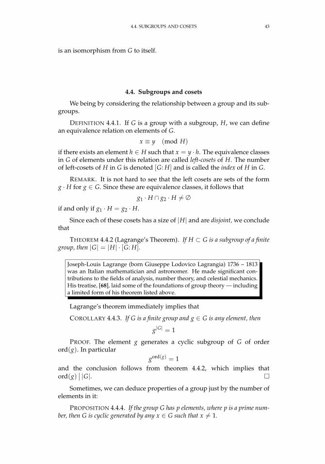
Joseph-Louis Lagrange (born Giuseppe Lodovico Lagrangia) 1736 – 1813was an Italian mathematician and astronomer. He made significant con-tributions to the fields of analysis, number theory, and celestial mechanics.His treatise, [68], laid some of the foundations of group theory — includinga limited form of his theorem listed above.
Lagrange’s theorem immediately implies that
COROLLARY 4.4.3. If G is a finite group and g ∈ G is any element, then
g|G| = 1
PROOF. The element g generates a cyclic subgroup of G of orderord(g). In particular
gord(g) = 1and the conclusion follows from theorem 4.4.2, which implies thatord(g)
∣∣ |G|.
Sometimes, we can deduce properties of a group just by the number ofelements in it:
PROPOSITION 4.4.4. If the group G has p elements, where p is a prime num-ber, then G is cyclic generated by any x ∈ G such that x 6= 1.
44 4. GROUP THEORY
PROOF. In x ∈ G, then ord(x) = 1 or p. If x 6= 1, ord(x) = p and thedistinct powers of x are all of the elements of G.
The equivalence relation in definition 4.4.1 on the previous page looksvery similar to that of definition 3.2.1 on page 18 so proposition 3.2.2 onpage 19 leads to the natural question
Does equivalence modulo a subgroup respect multiplication (i.e.,the group-operation)?
Consider what happens when we multiply sets of group-elements together.If H ⊂ G is a subgroup, then
H · H = H
— multiplying every element of H by every other element just gives usH back. This follows from the fact that 1 ∈ H and H is closed under thegroup-operation. If we multiply two cosets together
g1 · H · g2 · Hwe get a set of group-elements that may or may not be a coset. Note that
g1 · H · g2 · H = g1g2 · g−12 Hg2H
If g−12 Hg2 = H as a set, then
(4.4.1) g1H · g2H = g1g2H
This suggests making a few definitions
DEFINITION 4.4.5. If G is a group with a subgroup H ⊂ G and g ∈ G,then the conjugate of H by g is defined to be g · H · g−1, and denoted Hg.
A subgroup H ⊂ G of a group is said to be normal if H = Hg for allg ∈ G. This fact is represented by the notation H C G.
REMARK. For H to be a normal subgroup of G, we do not requireghg−1 = h for h ∈ H and every g ∈ G — we only require ghg−1 ∈ Hwhenever h ∈ H.
If G is abelian, all of its subgroups are normal becauseghg−1 = gg−1h = h.
Here’s an example of a non-normal subgroup:Let
S =
1, a =
(1 2 32 1 3
)⊂ S3
and let
g =
(1 2 31 3 2
)so that g2 = 1 which means g−1 = g. When we conjugate a by this, we get(
1 2 31 3 2
)(1 2 32 1 3
)(1 2 31 3 2
)=
(1 2 33 2 1
)/∈ S
PROPOSITION 4.4.6. If H C G is a normal subgroup of a group, then the setof left cosets forms a group.
4.4. SUBGROUPS AND COSETS 45
PROOF. Equation 4.4.1 on the facing page implies that
g1H · g2H = g1g2H
so the group identities for cosets follow from the identities in G: the identity element is
1 · Hthe inverse of g · H is
g−1 · H and
g1H(g2Hg3) = g1(g2g3)H
= (g1g2)g3H
= (g1Hg2H)g3H
This group of cosets has a name:
DEFINITION 4.4.7. If H C G is a normal subgroup, the quotient group,G/H, is well-defined and equal to the group of left cosets of H in G. The
mapp: G → G/H
that sends an element g ∈ G to its coset is a homomorphism — the projectionto the quotient.
If G = Z then G is abelian and all of its subgroups are normal. If H isthe subgroup n ·Z, for some integer n, we get
Z
n ·Z∼= Zn
In fact, a common notation for Zn is Z/nZ.If G = Zn and d
∣∣ n, we know that G has a subgroup isomorphic to Zd(see exercise 4.3.3 on page 41) and the quotient
Zn
Zd∼= Zn/d
Quotient groups arise naturally whenever we have a homomorphism:
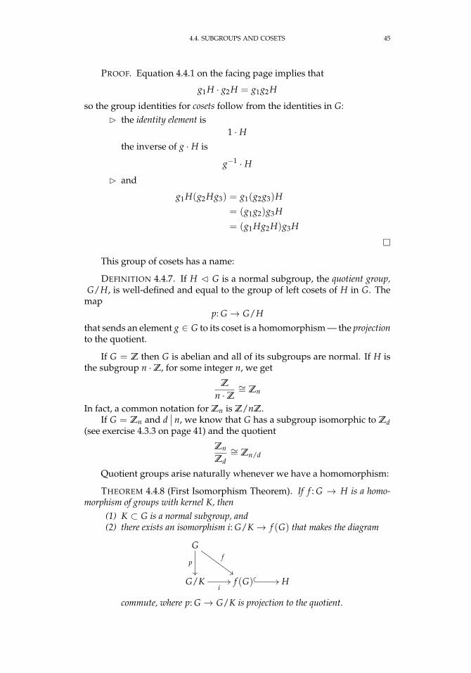
THEOREM 4.4.8 (First Isomorphism Theorem). If f : G → H is a homo-morphism of groups with kernel K, then
(1) K ⊂ G is a normal subgroup, and(2) there exists an isomorphism i: G/K → f (G) that makes the diagram
G
p
f
##
G/Ki// f (G)
// H
commute, where p: G → G/K is projection to the quotient.
46 4. GROUP THEORY
REMARK. The phrase “diagram commutes” just means that, as maps,f = i p.
If f is surjective, then H is isomorphic to G/K.
PROOF. We prove the statements in order. If k ∈ K and g ∈ G,
f (g · k · g−1) = f (g) · f (k) · f (g−1)
= f (g) · 1 · f (g)−1
= 1
so g · k · g−1 ∈ K and K is normal.Now we define i to send a coset K · g ⊂ G to f (g) ∈ H. First, we
have to show that this is even well-defined. If g′ ∈ g · K, we must show thatf (g′) = f (g). the fact that g′ ∈ K · g implies that g′ = g · k, for some k ∈ Kso
f (g′) = f (k) · f (g)
= 1 · f (g) = f (g)
Since (g1 · K)(g2 · K) = g1g2 · K , it is not hard to see that i is a hom-omorphism. It is also clearly surjective onto f (G). If i(K · g) = 1 ∈ H, itfollows that g ∈ K and g · K = 1 · K so that i is also injective.
Now we consider some special subgroups of a group:
DEFINITION 4.4.9. If G is a group, define Z(G) — the center of G — tobe the set of all elements x ∈ G such that xg = gx for all g ∈ G.
REMARK. Note that |Z(G)| ≥ 1 since 1 commutes with everything inG.
Since the elements of Z(G) commute with all of the elements of G, Z(G)is always a normal subgroup of G.
If H ⊂ G is a subgroup of a group, H is frequently not a normal sub-group. The normalizer of H is the largest subgroup of G containing H inwhich H is normal:
DEFINITION 4.4.10. If H ⊂ G is a subgroup of a group, the normalizerNG(H) is defined by
NG(H) =
g ∈ G∣∣∀h ∈ H, ghg−1 ∈ H
REMARK. In other words, gHg−1 = H, as sets.If g ∈ G is actually an element of H, we always have gHg−1 = H. This
means that H ⊂ NG(H) ⊂ G.
We can also define the normal closure or conjugate closure of a sub-group.
DEFINITION 4.4.11. If S ⊂ G is a subgroup of a group, its normal closure(or conjugate closure), SG, is defined to be the smallest normal subgroup ofG containing S. It is given by
SG = 〈sg for all s ∈ S and g ∈ G〉
4.4. SUBGROUPS AND COSETS 47
REMARK. The normal closure is the smallest normal subgroup of G thatcontains S.
We also have
DEFINITION 4.4.12. If g1, g2 ∈ G are elements of a group, their commu-tator [g1, g2] is defined by
[g1, g2] = g1g2g−11 g−1
2
and the commutator subgroup, [G, G], is defined by
[G, G] = 〈[g1, g2] for all g1, g2 ∈ G〉Some subgroups of a group are “more than normal:”
DEFINITION 4.4.13. If G is a group with subgroup, H, then H is said tobe a characteristic subgroup if, for any automorphism
f : G → G
f (H) = H.
REMARK. Characteristic subgroups are always normal, but not all nor-mal subgroups are characteristic. Usually characteristic subgroups are de-fined by some structural property that is preserved by all automorphisms.For instance, the center of a group (see definition 4.4.9 on the facing page)is characteristic.
We also have the interesting concept of the socle of a group:
DEFINITION 4.4.14. If G is a group, its socle, denoted Soc(G) is the sub-group generated by all minimal subgroups of G. If a group has no minimalsubgroups, its socle is the identity, 1.
REMARK. If G = Z12, generated by 1, then it has two minimal sub-groups, namely the one generated by 6 and isomorphic to Z2 and the onegenerated by 4, isomorphic to Z3. The socle is the subgroup generated by4, 6, which is the one generated by 2.
It is not hard to see that minimal subgroups and the socle are charac-teristic.
There are more isomorphism theorems that are proved in the exercises.
EXERCISES.
1. If H, K ⊂ G are subgroups of a group, HK stands for all products ofthe form h · k with h ∈ H and k ∈ K. This is not usually a subgroup of G. IfK is a normal subgroup of G, show that HK is a subgroup of G.
2. If H, K ⊂ G are subgroups of a group, where K is a normal subgroup,show that K is a normal subgroup of HK.
3. If H, K ⊂ G are subgroups of a group, where K is a normal subgroup,show that H ∩ K is a normal subgroup of H.
48 4. GROUP THEORY
4. If H, K ⊂ G are subgroups of a group, where K is a normal subgroup,show that
HKK∼= H
H ∩ KThis is called The Second Isomorphism Theorem.
5. If K C G is a normal subgroup and
p: G → G/K
is the projection to the quotient, show that there is a 1-1 correspondence be-tween subgroups of G/K and subgroups of G that contain K, with normalsubgroups of G/K corresponding to normal subgroups of G. This is calledthe Correspondence Theorem for groups.
6. If G is a group with normal subgroups H and K with K ⊂ H, thenH/K C G/K and
GH∼= G/K
H/KThis is called the Third Isomorphism Theorem.
7. Show that the set
S =
(1 2 31 2 3
),(
1 2 32 3 1
),(
1 2 33 1 2
)is a normal subgroup of S3. What is the quotient, S3/S?
8. Show that Z(G) ⊂ G is a subgroup.
9. If Z(G) is the center of a group G, show that Z(G) is abelian.
10. Suppose G is a group with normal subgroups H, K such that H ∩K = 0 and G = HK. Show that
G ∼= H ⊕ K
11. If G is a group with 4 elements, show that G is abelian.
12. If H ⊂ G is a subgroup of a group and g ∈ G is any element, showthat Hg is a subgroup of G.
13. If G is a group, show that conjugation by any g ∈ G defines an au-tomorphism of G. Such automorphisms (given by conjugation by elementsof the group) are called inner automorphisms.
14. Show that the automorphisms of a group, G, form a group them-selves, denoted Aut(G)
15. If m is an integer, show that Aut(Zm) = Z×m .
16. If G is a group show that the inner automorphisms of G form agroup, Inn(G) — a subgroup of all automorphisms.
17. If G is a group show that Inn(G) C Aut(G), i.e., the subgroup ofinner automorphisms is a normal subgroup of the group of all automor-phisms. The quotient is called the group of outer automorphisms.
Out(G) =Aut(G)
Inn(G)
4.5. SYMMETRIC GROUPS 49
18. If G is a group, show that the commutator subgroup, [G, G], is anormal subgroup.
19. If G is a group, show that the quotient
G[G, G]
is abelian. This is often called the abelianization of G.
20. If G is a group andp: G → A
is a homomorphism with A abelian and kernel K, then
[G, G] ⊂ K
so [G, G] is the smallest normal subgroup of G giving an abelian quotient.
4.5. Symmetric Groups
In the beginning of group theory, the word “group” meant a group ofpermutations of some set — i.e., a subgroup of a symmetric group. In somesense, this is accurate because:
THEOREM 4.5.1 (Cayley). If G is a group, there exists a symmetric groupSG and an injective homomorphism
f : G → SG
where SG is the group of all possible permutations of the elements of G.
Arthur Cayley (1821 – 1895) was a British mathematician noted for his con-tributions to group theory, linear algebra and algebraic geometry. His in-fluence on group theory was such that group multiplication tables (like thatin 4.1.1 on page 37) were originally called Cayley tables.
PROOF. First, list all of the elements of G
1, g1, g2, . . . If x ∈ G, we define the function f by
f (x) =(
1 g1 g2 . . .x x · g1 x · g2 . . .
)We claim that this is a permutation in SG: If x · gi = x · gj, then we canmultiply on the left by x−1 to conclude that gi = gj. Furthermore, everyelement of G occurs in the bottom row: if g ∈ G is an arbitrary elementof G, then it occurs under the entry x−1 · g in the top row. This function isinjective because f (x) = 1 implies that(
1 g1 g2 . . .x x · g1 x · g2 . . .
)= 1 =
(1 g1 g2 . . .1 g1 g2 . . .
)
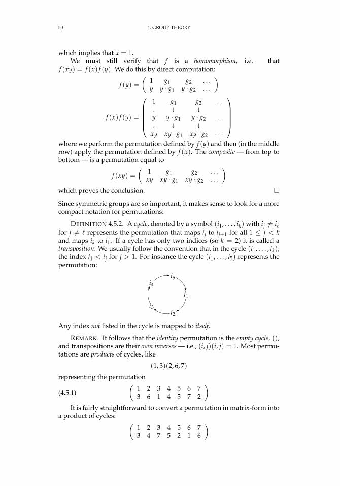
50 4. GROUP THEORY
which implies that x = 1.We must still verify that f is a homomorphism, i.e. that
f (xy) = f (x) f (y). We do this by direct computation:
f (y) =(
1 g1 g2 . . .y y · g1 y · g2 . . .
)
f (x) f (y) =
1 g1 g2 . . . y y · g1 y · g2 . . .
xy xy · g1 xy · g2 · · ·
where we perform the permutation defined by f (y) and then (in the middlerow) apply the permutation defined by f (x). The composite — from top tobottom — is a permutation equal to
f (xy) =(
1 g1 g2 . . .xy xy · g1 xy · g2 . . .
)which proves the conclusion.
Since symmetric groups are so important, it makes sense to look for a morecompact notation for permutations:
DEFINITION 4.5.2. A cycle, denoted by a symbol (i1, . . . , ik) with ij 6= i`for j 6= ` represents the permutation that maps ij to ij+1 for all 1 ≤ j < kand maps ik to i1. If a cycle has only two indices (so k = 2) it is called atransposition. We usually follow the convention that in the cycle (i1, . . . , ik),the index i1 < ij for j > 1. For instance the cycle (i1, . . . , i5) represents thepermutation:
i1
i2i3
i4i5
Any index not listed in the cycle is mapped to itself.
REMARK. It follows that the identity permutation is the empty cycle, (),and transpositions are their own inverses — i.e., (i, j)(i, j) = 1. Most permu-tations are products of cycles, like
(1, 3)(2, 6, 7)
representing the permutation
(4.5.1)(
1 2 3 4 5 6 73 6 1 4 5 7 2
)It is fairly straightforward to convert a permutation in matrix-form into
a product of cycles: (1 2 3 4 5 6 73 4 7 5 2 1 6
)
4.5. SYMMETRIC GROUPS 51
(1) Start with 1 and note that it maps to 3, so we get (1, 3, . . . ). Now,note that 3 maps to 7, giving (1, 3, 7, . . . ). Since 7 maps to 6, we get(1, 3, 7, 6, . . . ). Since 6 maps to 1, and 1 is already in the cycle weare constructing, our first cycle is complete:
(1, 3, 7, 6)
(2) Now delete those columns from the matrix representation in 4.5.1on the facing page to give(
2 4 54 5 2
)(3) And repeat the previous steps until all columns have been elimi-
nated. We get(1 2 3 4 5 6 73 4 7 5 2 1 6
)= (1, 3, 7, 6)(2, 4, 5)
which is much more compact than the matrix-representation.Step 2 above guarantees that the cycles we generate will have the property
DEFINITION 4.5.3. Two cycles a = (i1, . . . , is) and b = (j1, . . . , jt) aresaid to be disjoint if, as sets, i1, . . . , is ∩ j1, . . . , jt = ∅.
REMARK. Since a does not affect any of the elements that b permutesand vice-versa, we have ab = ba.
THEOREM 4.5.4. The symmetric group is generated by transpositions.
PROOF. A little computation shows that we can write every cycle as aproduct of transpositions:
(4.5.2) (i1, . . . , is) = (is−1, is) · · · (i2, is)(i1, is)
Recall exercise 5 on page 38, in which the reader showed that (ab)−1 =b−1a−1 . A simple induction shows that
(a1 . . . an)−1 = a−1
n · · · a−11
in any group. This fact, coupled with the fact that transpositions are theirown inverses means
(4.5.3) (i1, . . . , is) = (a1, b1) · · · (as−1, bs−1)(as, bs)
implies that
(4.5.4) (i1, . . . , is)−1 = (as, bs)(as−1, bs−1) · · · (a1, b1)
Since every permutation is a product of disjoint cycles, and every cyclecan be expressed as a product of transpositions, it follows that every permu-tation can be written as a product of transpositions. This representation isfar from unique — for instance a bit of computation shows that
(1, 2, 3, 4, 5) = (1, 5)(1, 4)(1, 3)(1, 2)
= (4, 5)(2, 5)(1, 5)(1, 4)(2, 3)(1, 4)(4.5.5)
52 4. GROUP THEORY
We can carry this result further
COROLLARY 4.5.5. The symmetric group, Sn, is generated by the transposi-tions
(1, 2), (1, 2), . . . , (1, n)
PROOF. By theorem 4.5.4 on the preceding page, it suffices to show thatevery transposition can be expressed in terms of the given set. We have:
(i, j) = (1, i)(1, j)(1, i)
It is possible to generate Sn with fewer than n generators:
COROLLARY 4.5.6. The symmetric group, Sn, is generated by the n− 1 ad-jacent transpositions
(1, 2), (2, 3), . . . , (n− 1, n)
PROOF. As before, we must show that any transposition, (i, j), can beexpressed in terms of these. We assume i < j and do induction on j− i. Ifj− 1 = 1 the transposition is adjacent and the result is true.
Now note that
(i, j) = (i, i + 1)(i + 1, j)(i, i + 1)
and j− (i + 1) < j− i so the induction hypothesis implies that (i + 1, j) canbe written as a product of adjacent transpositions.
Notice that the longer representation in equation 4.5.2 on the previouspage has precisely two more transpositions in it than the shorter one. Thisno accident — representing a more general phenomena. To study that, weneed the following
LEMMA 4.5.7. If
(4.5.6) 1 = (a1, b1) · · · (ak, bk) ∈ Sn
then k must be an even number.
PROOF. We will show that there exists another representation of 1 withk − 2 transpositions. If k is odd, we can repeatedly shorten an equationlike 4.5.6 by two and eventually arrive at an equation
1 = (α, β)
which is a contradiction.Let i be any number appearing in equation 4.5.6 and suppose the right-
most transposition in which i appears is tj = (i, bj) — so i = aj and i 6= a`, b`for all ` > j. We distinguish four cases:
(1) (aj−1, bj−1) = (aj, bj) = (i, bj). In this case (aj−1, bj−1)(aj, bj) =1 and we can simply delete these two permutations from equa-tion 4.5.6. We are done.
4.5. SYMMETRIC GROUPS 53
(2) (aj−1, bj−1) = (i, bj−1) where bj−1 6= bj, i. In this case, a little com-putation shows that
(aj−1, bj−1)(i, bj) = (i, bj)(bj−1, bj)
so that the index i now occurs one position to the left of where itoccurred before.
(3) (aj−1, bj−1) = (aj−1, bj), where aj−1 6= aj, bj. In this case
(aj−1, bj−1)(i, bj) = (i, bj−1)(aj−1, bj)
and, again, the index i is moved one position to the left.(4) The transpositions (aj−1, bj−1) and (i, bj) = (aj, bj) are disjoint, as
per definition 4.5.3 on page 51 in which case they commute witheach other so that
(aj−1, bj−1)(i, bj) = (i, bj)(aj−1, bj−1)
We use cases 2-4 to move the rightmost occurrence of i left until we en-counter case 1. This must happen at some point — otherwise we couldmove i all the way to the left until there is only one occurrence of it inall of equation 4.5.6 on the facing page. If this leftmost occurrence of i is ina transposition (i, i′), it would imply that the identity permutation maps i towhatever i′ maps to — which cannot be i since i doesn’t appear to the right ofthis transposition. This is a contradiction.
We are ready to prove an important result
PROPOSITION 4.5.8. If σ ∈ Sn is a permutation and
σ = (a1, b1) · · · (as, bs)
= (c1, d1) · · · (ct, dt)
are two ways of writing σ as a product of transpositions then
s ≡ t (mod 2)
PROOF. We will show that s + t is an even number. Equations 4.5.3and 4.5.4 on page 51 show that
σ−1 = (ct, dt) · · · (c1, d1)
so that1 = σ · σ−1 = (a1, b1) · · · (as, bs)(ct, dt) · · · (c1, d1)
and the conclusion follows from lemma 4.5.7 on the facing page.
So, although the number of transpositions needed to define a permuta-tion is not unique, its parity (odd or even) is:
DEFINITION 4.5.9. If n > 1 and σ ∈ Sn is a permutation, then the parityof σ is defined to be even if σ is equal to the product of an even number oftranspositions, and odd otherwise. We define the parity-function
℘(σ) =
0 if σ is even1 if σ os odd
54 4. GROUP THEORY
REMARK. Equation 4.5.2 on page 51 shows that cycles of even length(i.e., number of indices in the cycle) are odd permutations and cycles of oddlength are even.
If σ ∈ Sn is a permutation, equation 4.5.4 on page 51 implies ℘(σ−1) =℘(σ). By counting transpositions, it is not hard to see that:
(1) The product of two even permutations is even,(2) The product of an even and odd permutation is odd,(3) The product of two odd permutations is even.
This implies that the even permutations form a subgroup of the symmetricgroup:
DEFINITION 4.5.10. If n > 1 the subgroup of even permutations of Snis called the degree-n alternating group An.
REMARK. The parity-function defines a homomorphism
℘: Sn → Z2
whose kernel is An.
It is fairly straightforward to compute conjugates of cycles:
PROPOSITION 4.5.11. If σ ∈ Sn is a permutation and (i1, . . . , ik) ∈ Sn is acycle, then
(i1, . . . , ik)σ = (σ(i1), . . . , σ(ik))
PROOF. Recall that
(i1, . . . , ik)σ = σ (i1, . . . , ik) σ−1
If x /∈ σ(i1), . . . , σ(ik), then σ−1(x) /∈ i1, . . . , ik so (i1, . . . , ik)σ−1(x) =
σ−1(x) andσ (i1, . . . , ik) σ−1(x) = x
On the other hand, if x = σ(ij), then σ−1(x) = ij and (i1, . . . , ik) σ−1(x) = ij+1 (unless j = k, in which case we wrap around to i1) and
σ (i1, . . . , ik) σ−1(σ(ij)) = σ(ij+1)
COROLLARY 4.5.12. The cycles (i1, . . . , is), (j1, . . . , jt) ∈ Sn are conjugateif and only if s = t.
PROOF. Proposition 4.5.11 implies that s = t if they are conjugate. Ifs = t, proposition 4.5.11 shows that
(j1, . . . , js) = (i1, . . . , is)(i1,j1)···(is ,js)
Here, we follow the convention that (iα, jα) = () if iα = jα.
Just as Sn is generated by transpositions, we can find standard genera-tors for alternating groups:
PROPOSITION 4.5.13. The alternating group, An, is generated by cycles ofthe form (1, 2, k) for k = 3, . . . , n.
4.5. SYMMETRIC GROUPS 55
PROOF. The group, An, is generated by pairs of transpositions:(a, b)(c, d) or (a, b)(b, c) but
(a, b)(c, d) = (a, c, b)(a, c, d)
(a, b)(b, c) = (a, c, b)
so we know that An is generated by cycles of length 3. Now, note that(1, a, 2) = (1, 2, a)−1 and (1, a, b) = (1, 2, b)(1, 2, a)−1. In addition,(2, a, b) = (1, 2, b)−1(1, 2, a).
With these basic cases out of the way, we are in a position to handle thegeneral case. If a, b, c 6= 1, 2, a slightly tedious calculation shows that
(a, b, c) = (1, 2, a)−1(1, 2, c)(1, 2, b)−1(1, 2, a)
which proves the result.
DEFINITION 4.5.14. A group, G, is defined to be simple if it has no nor-mal subgroups other than 1 and G itself.
REMARK. It is not hard to find examples of simple groups: if p is aprime number, Zp is simple since it doesn’t have any subgroups other than0 and Zp. One reason that simple groups are interesting is that one canconstruct all finite groups out of them.
For many years, the classification of all finite simple groups was oneof the most famous unsolved problems in group theory. It was solved ina series of several hundred papers published between 1955 and 2004 —involving thousands of pages of logical reasoning.
THEOREM 4.5.15. If n 6= 4, the group An is simple.
PROOF. If n = 3, A3 = Z3 so it is simple. If n = 4 , A4 has the subgroup
1, (1, 2)(3, 4), (1, 3)(2, 4), (1, 4)(2, 3)which can be verified to be normal, so A4 is not simple. Now supposen ≥ 5.
Suppose H ⊂ An is a normal subgroup. If (1, 2, 3) ∈ H, then propo-sition 4.5.11 on the preceding page implies that (1, 2, 3)(3,k) = (1, 2, k) andthis conjugate must be contained in H because H is normal. Since these cy-cles generate An (see proposition 4.5.13 on the facing page) it follows thatH = An. If H has any 3-cycle, corollary 4.5.12 on the preceding page showsthat this 3-cycle is conjugate to (1, 2, 3) so that (1, 2, 3) ∈ H and H = An.
Now we show that, if n > 4, H ⊂ An must have a 3-cycle so thatH = An. We consider the elements of H — products of disjoint cycles:
x = c1 · · · cr
Case 1: At least one of the ci has length ≥ 4 — i.e. ci = (i1, . . . , ik)τ ∈ H,where k ≥ 4 and τ is disjoint from (i1, . . . , ik). The normality of Hand corollary 4.5.12 on the facing page means that it also containsσ = (1, 2, . . . , k)τ′ and
σ−1σ(1,2,3) = (1, 2, k)
which implies that H = An.
56 4. GROUP THEORY
Case 2: x has at least two cycles of length 3 — i.e., x = (i1, i2, i3)(j1, j2, j3)τwhere τ is disjoint from the cycles. Proposition 4.5.11 on page 54and the fact that H is normal shows that, without loss of general-ity, we can assume x = (1, 2, 3)(4, 5, 6)τ. Let σ = (1, 2, 4). Then σcommutes with τ so
xσ = [(1, 2, 3)(4, 5, 6)]στ
= (1, 2, 3)σ(4, 5, 6)στ
= (2, 4, 3)(1, 5, 6)τ
Then
xσx−1 = (2, 4, 3)(1, 5, 6)ττ−1(4, 5, 6)−1(1, 2, 3)−1
= (2, 4, 3)(1, 5, 6)(4, 6, 5)(1, 3, 2)
= (1, 2, 5, 3, 4)
which shows that H has a cycle of length ≥ 4 — and this takes usback to case 1.
Case 3: x has one cycle of length 3 and all of the others have length 2. With-out loss of generality, we can assume x = (1, 2, 3)τ. Since cycles oflength 2 are their own inverses we have τ2 = 1 and x2 = (1, 3, 2)— which implies that H = An.
Case 4: x consists entirely of disjoint transpositions — so, for instance, x2 =1. Without loss of generality, we can assume
x = (1, 2)(3, 4)τ
If σ = (1, 2, 3), we have
xσ = σxσ−1
= (1, 2)σ(3, 4)στ
= (2, 3)(1, 4)τ
and
xσx−1 = (2, 3)(1, 4)ττ−1(3, 4)(1, 2)
= (2, 3)(1, 4)(3, 4)(1, 2)
= (1, 3)(2, 4)
so we conclude that α = (1, 3)(2, 4) ∈ H (i.e., without any τ-factor).Proposition 4.5.11 on page 54 shows that
α(1,3,5) = (3, 5)(2, 4)
and we have
αα(1,3,5) = (1, 3)(2, 4)(3, 5)(2, 4)(4.5.7)
= (1, 3, 5)
so (1, 3, 5) ∈ H and H = An. Note that the (2, 4)-transpositionsin equation 4.5.7 are disjoint from the others and just cancel eachother out.
4.5. SYMMETRIC GROUPS 57
We can use symmetric groups and permutations to analyze othergroups.
Recall the group, D8, defined in table 4.1.1 on page 37 — the group ofsymmetries of the square.
EXAMPLE 4.5.16. The general dihedral group D2n is the group of sym-metries of a regular n-sided polygon.
These symmetries are: rotations by 2π/n — giving rise to an element r ∈ D2n with rn = 1. when n is even, we have reflections through axes through two
corners (the dotted lines in figure 4.1.2 on page 36), giving rise tofi ∈ Dn, i = 1, . . . , n with f 2
i = 1. In this case, f1 = (2, n)(3, n−1) · · · (k, k + 2) as a permutation of vertices.
In the odd case n = 2k+ 1, fi is a reflection through vertex i and themidpoint of the face (k+ 1, k+ 2), and f1 = (2, n)(3, n− 1) · · · (k+1, k + 2), as a permutation of vertices.
if n = 2k, we also have reflections through axes passing throughmidpoints of two opposite faces (the dashed lines in figure 4.1.2 onpage 36). These give rise to elements gi ∈ Dn, i = 1, . . . , n withg2
i = 1. It appears that we have 2n reflections in all but the sym-metry of the even case implies that f1, . . . , fk = fk+1, . . . , fnand g1, . . . , gk = gk+1, . . . , gn as sets, so that, again, we have nreflections in all.
In all cases, proposition 4.5.11 on page 54 shows that
r f1 = (1, n, n− 1, . . . , 2) = r−1 = rn−1
PROPOSITION 4.5.17. If n > 2, D2n is generated by r and f1 and the ele-ments of D2n are precisely
1, r, . . . , rn−1, f1, r f1, . . . , rn−1 f1
so it is of order 2n and defined by the equations rn = 1, f 2
1 = 1, and r f1 = r−1.
REMARK. In a rather confusing convention, the dihedral group D2nis sometimes written as Dn (especially where its geometric properties arebeing studied).
PROOF. We have already seen 2n potential elements of D2n: the ro-tations and reflections. The relations f 2
1 = 1 and r f1 = rn−1 imply thatf1r f1 = rn−1 so that f1rk f1 = rk(n−1), which implies that
f1rk = rk(n−1) f1
and this exhausts possible products of r and f1. It is not hard to see thatthese are all distinct. An arbitrary product
f1rn1 · · · f1rnk f i1
can be rewritten as rt f s1 .

58 4. GROUP THEORY
1
2
34
5
FIGURE 4.5.1. Regular pentagon
EXERCISES.
1. Convert (1 2 3 4 5 6 7 8 93 1 6 9 4 7 2 5 6
)to cycle notation
2. Is the permutation(1 2 3 4 5 6 7 8 99 1 6 3 4 7 6 5 2
)odd or even?
3. If g ∈ Sn is an element we arrange the disjoint cycles of g in orderfrom longest to shortest (and list elements that are fixed by g as cycles oflength 1):
g = (a1, . . . , ak1)(b1, · · · , bk2) · · · (z1, . . . , zkt)
and call the sequence of numbers k1 ≥ k2 ≥ · · · ≥ kt, the cycle structure ofg. Show that two elements of Sn are conjugate if and only if they have thesame cycle structure.
4. What is the center of S3?
5. Represent the dihedral group, D8 — see 3.2.2 on page 20 — as asubgroup of S4.
6. Let G ⊂ S5 be a subgroup containing a 5-cycle and a transposition.Show that this implies that G = S5.
4.6. Abelian Groups
There are a “islands of success” in mathematics — areas that are “com-pletely solved:” Every reasonable question one has can be answered. Thetheory of finitely generated abelian groups is one of these areas.
We begin with free abelian groups:
4.6. ABELIAN GROUPS 59
DEFINITION 4.6.1. A group, A, is a free abelian group if it has a gener-ating set
X = x1, . . . that is linearly independent — i.e. any equation
(4.6.1)n
∑i=1
akixki
= 0
where ai ∈ Z, implies that ak1 = · · · = akn = 0. If the set X is finite, itsorder is called the rank of A. This generating set is called a free basis of A.
REMARK. The word “free” is used because equation 4.6.1 implies thatthe basis do not satisfy any equations other than those dictated by simplelogic (and the fact that the groups are abelian). If B is any abelian group,this freeness property means that any map of the basis elements
f (xi) = bi ∈ B
gives rise to a unique homomorphism
f : A→ B
f
(n
∑i=1
nixi
)=
n
∑i=1
nibi(4.6.2)
At this point, we come up against the distinction between a direct sum(as in definition 4.1.12 on page 38) and direct product.
DEFINITION 4.6.2. Given an infinite set of abelian groups Ai(1) their direct product
∞
∏i=1
Ai
is the set of all infinite sequences
(a1, a2, . . . )
with ai ∈ Ai.(2) their direct sum
∞⊕i=1
Ai
is the set of infinite sequences
(a1, a2, . . . )
in which only a finite number of the ai are nonzero.
REMARK. When a finite number of groups are involved, direct prod-ucts are identical to direct sums. When an infinite number of groups areinvolved, they become very different and
∞⊕i=1
Ai ⊂∞
∏i=1
Ai
In a category-theoretic sense (see chapter 10 on page 335) direct productsare products (see definition 10.1.1 on page 335) in the category of abeliangroups and direct sums are coproducts (see definition 10.1.4 on page 338).
60 4. GROUP THEORY
Using direct sums, we can characterize free abelian groups:
PROPOSITION 4.6.3. If X is a set and A is a free abelian group with X as abasis, then there exists an isomorphism
f :⊕x∈X
Zx → A
REMARK. This is true whether X is finite or infinite. Note that Zx rep-resents a copy of Z indexed by x ∈ X.
PROOF. Just define
f (n1, . . . ) = n1x1 + · · ·The fact that the xi are linearly independent in A implies that this map isinjective. The fact that every element of A is a finite linear combination ofthe xi ∈ X implies that it is surjective.
It follows that the infinite direct sum∞⊕
i=1
Z
is a free abelian group.We can also define
DEFINITION 4.6.4. The infinite direct product
B =∞
∏i=1
Z
is called the Baer-Specker group.
REMARK. In exercises 3 through 6 on page 73, the reader will get achance to prove that this group is not free abelian. This group first appearedin Baer’s paper [9] in which he proved it was not free abelian2. Specker laterpublished the paper [100] which explored its rather bizarre properties.
COROLLARY 4.6.5. If A is a free abelian group of rank n, B is a free abeliangroup of rank m and if
A ∼= Bis an isomorphism, then n = m.
REMARK. In other words the rank of a finitely generated free abeliangroup is well-defined.
PROOF. The isomorphism A ∼= B induces an isomorphism
A2A
= Zn2∼= B
2B= Zm
2
forcing n = m.
The property of freeness of an abelian group is hereditary in the sensethat all of its subgroups inherit it:
2The proof in the exercises is simpler.
4.6. ABELIAN GROUPS 61
PROPOSITION 4.6.6. If S ⊂ A is a subgroup of a free abelian group, then Sis free abelian. If rank(A) < ∞, then
rank(S) ≤ rank(A)
REMARK. Compare this result with example 4.10.24 on page 103. Theessential difference is that A is free abelian.
PROOF. Let X be a free basis for A. By the Well Ordering Axiom of settheory (see axiom A.2.9 on page 461), we can order the elements of X
x1 x2 · · ·so that every subset of X has a minimal element. Note that this ordering iscompletely arbitrary — we only use the fact that such an ordering exists3.
If s ∈ S, we haves = ∑ nixi
— a finite sum. Define the leading term, λ(s) = nαxα — the highest orderedterm in the sum. Let Y ⊂ X be the set of basis elements that occur in theseleading terms of elements of S. For each y ∈ Y, there is at least one s ∈ Swhose leading term is n · y. Let
(4.6.3) I(y) = 0 ∪ n ∈ Z|λ(s) = n · y for some s ∈ SIt is not hard to see that
I(y) ⊂ Z
is a cyclic subgroup (see proposition 4.3.2 on page 41). If ny is the positivegenerator4 of I(y), there exists a set of elements Sy ⊂ S whose leading termsare nyy. The Axiom of Choice (see theorem A.2.11 on page 461) impliesthat we can select one such element for each y ∈ Y — i.e. we can define afunction
f : Y → Swhere f (y) is some (arbitrarily selected) element of Sy. We claim that theset
B = f (y)|y ∈ Yis a basis for S. We must demonstrate two things:
(1) the set B is linearly independent. This follows immediately from thefact that its leading terms are multiples of distinct basis elementsof A. If we have a linear combination
n
∑i=1
niyi + H = 0
where H is the non-leading terms. Of those leading terms, one isordered the highest — say nαyα and it can never be canceled outby any other term. It follows that nα = 0 and a similar argumentapplied to the remaining terms eventually leads to the conclusionthat all of the coefficients are 0.
3If X is finite, this is completely trivial; if X = R, not so much. The hard part is that everysubset must have a minimal element. See remark A.2.10 on page 461.
4Both ny and −ny are generators of the same cyclic subgroup of Z.
62 4. GROUP THEORY
(2) the set B generates S. Suppose not and suppose g ∈ S \ 〈B〉 hasthe property that λ(g) = my for m ∈ Z and y ∈ Y is minimal (inthe ordering on X — axiom A.2.9 on page 461). Then m ∈ I(g)(see equation 4.6.3 on the previous page) so that m = k · ng andk · f (y) ∈ 〈B〉 also has leading term my. It follows that
g− k · f (y) ∈ S \ 〈B〉has a leading term strictly lower than that of g — a contradiction.
It is interesting that every abelian group is a quotient of a free abeliangroup:
PROPOSITION 4.6.7. If A is any abelian group, there exists a surjective hom-omorphism
f : F → Awhere F is free abelian. If A is finitely generated then F can be of finite rank.
REMARK. Proposition 4.6.6 on the preceding page implies that the ker-nel of this map is also free so proposition 4.4.8 on page 45 implies thatevery abelian group is a quotient of a free abelian group by a free abeliansubgroup.
PROOF. Just define F to be the free abelian group on the basis A \ 0.The map f sends the basis element a ∈ A \ 0 to a ∈ A, and we extendthis map of basis elements to all of F via an analogue to equation 4.6.2 onpage 59.
If A has a finite generating set S = a1, . . . , an, we can define F to bea free abelian group whose basis is precisely S. The same argument as thatused above constructs the homomorphism f .
Our structure-theorem for finitely generated abelian groups is:
THEOREM 4.6.8. If A is a finitely generated abelian group, then
(4.6.4) A ∼= F⊕Zn1 ⊕ · · · ⊕Znk
where F is free-abelian and n1∣∣ n2
∣∣ · · · ∣∣ nk.
REMARK. Finite generation is essential to this result. When an abeliangroup is not finitely generated the result fails — see example 4.6.14 onpage 67.
PROOF. Let a1, . . . , an be a generating set for A. Define G to be thefree-abelian group on basis x1, . . . , xn and define the surjective homo-morphism
f : G → Axi 7→ ai
Proposition 4.6.6 on the preceding page implies that the kernel, K is also freeabelian on some basis y1, . . . , ym, where m ≤ n and proposition 4.4.8 onpage 45 implies that
A ∼= GK
4.6. ABELIAN GROUPS 63
If
yi =n
∑j=1
ai,jxj
the m× n matrix M = [ai,j] expresses how K fits in G and the quotient. Weconsider ways of “simplifying” this matrix in such a way that the quotientG/K remains unchanged:
(1) Rearranging the rows of M corresponds to re-labeling the yi, so itleaves G/K unchanged.
(2) Rearranging the columns of M corresponds to re-labeling the xj,leaving G/K unchanged.
(3) Multiplying a row by −1 defines an automorphism of K (see defi-nition 4.2.3 on page 40), leaving G/K unchanged.
(4) Multiplying a column by −1 defines an automorphism of G, leav-ing G/K unchanged.
(5) Adding a multiple of the ith row to the jth row (with i 6= j) de-fines an automorphism of K — we replace the basis y1, . . . , ymby y1, . . . , y′j, . . . , ym where y′j = yj + n · yi, where n is the multi-plying factor. This is invertible because yj = y′j− n · yi so it definesan isomorphism that doesn’t change the subgroup H ⊂ G or thequotient.
(6) For the same reason, adding a multiple of the ith column to the jth
column (with i 6= j) defines an automorphism of G that leaves thequotient, G/K, unchanged.
It follows that we can perform all of the operations listed above to M with-out changing the quotient in any way.
We’ll call this part of our algorithm, Diagonalization:This consists of two phases: row-reduction and column-reduction.We will call the (1, 1) position in the matrix, the pivot.By performing operations 1, 2, and 3 if necessary, we can assume that
a1,1 > 0. Now we scan down column 1.(1) If a1,1|ak,1 with k > 1, we subtract (a1,1/ak,1)× row 1 from row k,
replacing ak,1 by 0.(2) If a1,1 - ak,1, perform two steps:
(a) write ak,1 = q · a1,1 + r with 0 < r < a1,1. Now subtract q×row 1 from row k, replacing ak,1 by r.
(b) Swap row 1 with row k so that a1,1has been replaced by r.We perform step 2 until the matrix-entry in position (k, 1) is 0. Since thepivot position decreases every time we do step 2, we can only do it a finitenumber of times. The astute reader will recognize repetition of step 2 aboveas the Euclidean algorithm (see algorithm 3.1.4 on page 14) for computingthe greatest common divisor.
The effect is5:
a1,1 → gcd(a1,1, ak,1)
ak,1 → 0
5Where the symbol ‘→’ means “is replaced by.”
64 4. GROUP THEORY
Repeating these operations for all lower rows ultimately clears all elementsof column 1 below a1,1 to 0. This completes row-reduction for column 1.
Now we do column-reduction on row 1, ultimately clearing out all ele-ments to the right of a1,1 to 0.
After these steps, our matrix looks like[a1,1 00 M
]where M is an (m− 1)× (n− 1) matrix.
After recursively carrying out our algorithm above on this and thesmaller sub-matrices that result, we get the diagonal form:
a1,1 0 0 · · · 00 a2,2 0 · · · 0...
.... . . · · · ...
0 0 0 · · · 0
where all off-diagonal entries are 0 and we have n − m columns of 0’s onthe right. This matrix means that the new bases for K and F satisfy
yi = ai,i · xi
for 1 ≤ i ≤ m. This completes the phase of the algorithm called diagonal-ization.
Now we may run into the problem ai,i - ai+1,i+1. We can resolve this asfollows:
The subgroup of A determined by these two rows of the matrix hasai,i · ai+1,i+1 elements. Now add column i + 1 to column i to give[
ai,i 0ai+1,i+1 ai+1,i+1
]If we row-reduce this, a tedious calculation shows that we get[
δ u0 v
]where δ = gcd(ai,i, ai+1,i+1) and u and v are linear combinations of ai,i andai+1,i+1. At this point, we subtract (u/δ)× column i from column i + 1 toget [
δ 00 v
]Since the subgroup of A determined by these two rows is unchanged, itstill has ai,i · ai+1,i+1 elements. This means δ · v = ai,i · ai+1,i+1 so
v =ai,i · ai+1,i+1
δ= lcm(ai,i, ai+1,i+1)
On the other hand, the number of distinct prime factors in δ must be strictlyless than those in ai,i and ai+1,i+1 (equality only occurs if ai,i and ai+1,i+1have the same prime factors). So this operation shifts prime factors to theright and down.
4.6. ABELIAN GROUPS 65
After a finite number of steps, a1,1 must stabilize (i.e. remain constantover iterations of this process) since it has a finite number of prime factors.One can say the same of a2,2 as well. Eventually the entire list of elements
a1,1, . . . , am,mmust stabilize, finally satisfying the condition
a1,1∣∣ · · · ∣∣ am,m
When we form the quotient
A ∼= GK
=Z⊕Z⊕ · · · ⊕Z
a1,1 ·Z⊕ a2,2 ·Z⊕ · · · ⊕Z
=Z
a1,1 ·Z⊕ Z
a2,2 ·Z⊕ · · · ⊕Z
each nonzero entry ai,i results in a direct summand Zai,i = Z/ai,i ·Z, if ai,i 6= ±1 and 0 otherwise.
each column of zeros contributes a direct summand of Z to F inequation 4.6.4 on page 62.
If an abelian group is finite, the F-factor is zero and, in light of exercise 7on page 40, we conclude that
COROLLARY 4.6.9. If A is a finite abelian group, then
(4.6.5) A ∼= Zp
k11⊕ · · · ⊕Zpkn
n
where the pi are (not necessarily distinct) primes.
PROOF. Simply factor each ni in equation 4.6.4 on page 62 into powersof primes.
We summarize and extend these results with:
THEOREM 4.6.10. If A is a finite abelian group, then
A ∼= ∏i
Zpi ⊕ · · · ⊕Zpi︸ ︷︷ ︸αi,1 factors
⊕Zp2i⊕ · · · ⊕Zp2
i︸ ︷︷ ︸αi,2 factors
⊕ · · · ⊕Zp
tii⊕ · · · ⊕Z
ptii︸ ︷︷ ︸
αi,tifactors
where the (finite number of) primes, pi, and the integers αi,j are uniquely deter-mined by A.
REMARK. Of course many of the αi,j may be zero.
PROOF. We get the equation above from equation 4.6.5 by arrangingthe factors in order by primes and their powers. The only additional thingsto be proved are the statements regarding the primes pi and the integersαi,j.
If p and q are distinct primes, then for any integers i, k > 0
qk×: Zpi → Zpi
66 4. GROUP THEORY
is an isomorphism (see exercise 3 on page 42), so its kernel is 0. In addition,the kernel of
p×: Zpk → Zpk
is isomorphic to Zp (generated by pk−1 ∈ Zpk ).Consider the map
pji×: A→ A
and call its kernel Apj
iand its image pj
i A. Factors corresponding to primes
other than pi will not appear in the kernels of these multiplication-mapsbecause they are mapped isomorphically. Then any isomorphism
f : A→ A′
induces isomorphisms
f |Apj
i: A
pji→ A′
pji
f : pji A→ pj
i A′
Now note thatApi∼= Zpi ⊕ · · · ⊕Zpi︸ ︷︷ ︸
αi,1+αi,2+··· factors
because every factor of Zpj
i(regardless of j) gives rise to a copy of Zpi in
the kernel. Multiplying by pi kills off all copies of Zp1i
and we get
(pi A)pi∼= Zpi ⊕ · · · ⊕Zpi︸ ︷︷ ︸
αi,2+αi,3+··· factors
In general
|(pj−1i A)pi | = p
αi,j+αi,j+1+···i
so we can compute αi,j via
pαi,ji =
|(pj−1i A)pi ||(pj
i A)pi |Any isomorphism of A will map all of these groups derived from it
isomorphically, and preserve all of the αi,j.
Given any positive integer, n, we could list all of the isomorphismclasses of abelian groups of order n. For instance, if n = 8 we get
Z2 ⊕Z2 ⊕Z2
Z4 ⊕Z2
Z8
DEFINITION 4.6.11. A group, G, is torsion free if it has no elements offinite order.
Theorem 4.6.8 on page 62 immediately implies that
PROPOSITION 4.6.12. A finitely generated torsion free abelian group is free.
4.6. ABELIAN GROUPS 67
REMARK. This requires finite generation. For instance Q under additionis torsion free but definitely not free abelian: If q1, q2, . . . is any generatingset with qi ∈ Q, let q1 = a1/b1 and q2 = a2/b2 where a1, a2, b1, b2 ∈ Z. Then
(b1a2) · q1 − (b2a1) · q2 = 0
which implies that this arbitrary generating set is not linearly independent.
We need the following result to prove several other things in the future:
LEMMA 4.6.13. Let G be an abelian group with subgroups A and B. Thenwe have an isomorphism
A⊕ B((1⊕−1) ∆)(A ∩ B)
∼= A + B ⊂ G
where∆: A ∩ B→ A⊕ B
is the diagonal embedding defined by ∆(x) = x⊕ x for all x ∈ A ∩ B, and
(1⊕−1): A⊕ B→ A⊕ B
sends (a, b) to (a,−b) for all a ∈ A and b ∈ B.
REMARK. In particular, whenever G = A + B and A ∩ B = 0, G ∼=A⊕ B.
In the nonabelian case, this result fails — see definition 4.7.15 onpage 79.
PROOF. Consider the map
A⊕ B→ A + B
defined by(a, b) 7→ a + b
The kernel of this map is(c,−c)
where c ∈ A ∩ B, so Proposition 4.4.8 on page 45 implies
A + B =A⊕ B
((1⊕−1) ∆)(A ∩ B)
When groups are not finitely generated, their behavior becomes morecomplicated. For instance we have a counterexample to theorem 4.6.8 onpage 62:
EXAMPLE 4.6.14. Let p be a prime number and define
G =∞
∏k=1
Zp2k
This group is not torsion because it has elements of infinite order like
(1, 1, 1, . . . )
We claim that its torsion subgroup, tG, is not a direct summand. If so, therewould be a subgroup of G isomorphic to G/tG (as per lemma 4.6.13).
68 4. GROUP THEORY
Note that all elements of G are divisible by, at most, a finite power of p,i.e.
x = (n1 pk1 , n2 pk2 , . . . )
where all of the ni are relatively prime to p, is a multiple of pn with n =min(k1, . . . ) and no higher power of p. On the other hand, we claim thereare elements of G/tG divisible by arbitrarily high powers of p:
Let x = (p, p2, . . . , pk, . . . ), let j > 0 be an integer, and lety = (y1, . . . , yk, . . . )
yk =
pk−j if k ≥ j0 otherwise
Thenx− pjy = (p, p2, . . . , p2j−2, 0, 0, . . . )
has order p2j−2 and is, therefore, torsion. It follows that the element ofG/tG represented by x cannot be any element of G.
DEFINITION 4.6.15. If G is a torsion abelian group and p is a prime,its p-primary component, Gp is the subgroup of elements x ∈ G such thatpk · x = 0 for some integer k > 0.
We can prove a limited version of theorem 4.6.10 on page 65 for groupsthat may not be finitely generated:
THEOREM 4.6.16. If G is a torsion abelian group, then G is a direct sum ofits p-primary components for all primes p:
G ∼=⊕
pGp
PROOF. Suppose x has order
n = pk11 · · · p
ktt
The integers
ni = pk11 · · · p
ktt︸ ︷︷ ︸
omit ith factor
have a greatest common divisor of 1 so that there exist integers mi such that
1 = ∑ mini
We conclude thatx = ∑ mini · x
and ni · x has order pkii . It follows that
G = ∑p
Gp
The conclusion follows from lemma 4.6.13 on the preceding page and thefact that Gp ∩ Gp′ = 0 whenever p, p′ are distinct primes.
4.6. ABELIAN GROUPS 69
4.6.1. Divisible groups. This is a class of groups that is used in category the-ory and cohomology. All groups will be assumed to be abelian.
DEFINITION 4.6.17. A group G is divisible if every element is an arbitrary mul-tiple of some other element, i.e., if x ∈ G and n > 0 is an integer, then
x = ny
for some y ∈ G.
REMARK. For example, Q, R, and Q/Z are clearly divisible.
PROPOSITION 4.6.18. Divisible groups have the following properties(1) sums and products of divisible groups are divisible, and(2) quotients of divisible groups are divisible
PROOF. IfD = ∏ Di
is a product of divisible groups and x ∈ D is and element and n > 0 is an integer,then
x = (d1, . . . )and each component, di, of x can be ‘divided’ by n, so the same is true of x. If allbut a finite number of the di are 0, the same reasoning applies (where the result of‘dividing’ 0 by n is 0).
If D is divisible with a subgroup, S, and
G =DS
we can ‘divide’ x ∈ G by lifting it to D, dividing it there, and projecting back toG.
The following general result will be useful
LEMMA 4.6.19 (Pasting lemma). Let C be an abelian group with subgroups A andB and
f : A→ Cg: B→ C
are homomorphisms of groups with the property that
f |A ∩ B = g|A ∩ B
then there exists a unique extension f + g to , A + B ⊂ C, defined by
( f + g)(a + b) = f (a) + g(b)
for a ∈ A and b ∈ B.
REMARK. A corresponding result holds for nonabelian groups but is muchmore complicated.
PROOF. Lemma 4.6.13 on page 67 implies that
f ⊕ g: A⊕ B→ A + B
has kernel((1⊕−1) ∆)(A ∩ B)
The hypotheses imply that
f ⊕ g|((1⊕−1) ∆)(A ∩ B) = 0
so it factors through the quotient.
70 4. GROUP THEORY
The following result gives one of the most significant properties of divisiblegroups:
THEOREM 4.6.20. An abelian group D is divisible if and only if it satisfies the “injec-tivity condition:”
Any homomorphism f : A → D from any abelian group, A, extends toany group containing A. In other words, if A ⊂ B and
f : A→ D
is a homomorphism, there exists a homomorphism
F: B→ D
such that
F|A = f
REMARK. See propositions 10.5.5 on page 359 and 10.5.6 on page 359 for ageneralization of this argument.
PROOF. Suppose D satisfies this condition. If n > 0 is an integer and x ∈ D,we can define a mapping
fx: Z → D1 7→ x
Since Z can be regarded as the subgroup A = n · Z ⊂ Z = B, the injectivitycondition implies that fx extends to a map
F: Z→ D
and F(1) ∈ D is an element such that x = n · F(1), so D is divisible.Conversely, suppose D is divisible. Let P be the partially ordered set of ele-
ments (C, g) whereA ⊂ C
and g|A = f . This contains, at least, (A, f ). Any tower of elements (Cα, gα) hasan upper bound (⋃
Cα,∪gα
)Zorn’s lemma ( A.2.12 on page 462) implies that it has a maximal element (C, g).We claim that C = B.
If not, there exists x ∈ B \ C. Consider its image, x, in the quotient, B/C. If theorder of x is infinite, then
〈x〉 ∩ C = 0so that lemma 4.6.13 on page 67 implies that
C + 〈x〉 ∼= C⊕ 〈x〉and we can extend g to g ⊕ 0:∼= C ⊕ 〈x〉 → D, contradicting the maximality of(C, g) .
On the other hand, suppose x has order n in B/C. Then nx ∈ C. Since D isdivisible, there exists a y ∈ D such that n · y = g(n · x).
Lemma 4.6.19 on the preceding page implies that g can be extended to
g′: C + 〈x〉 → Dx 7→ y
which also contradicts the maximality of (C, g) .
This has a number of interesting implications:
4.6. ABELIAN GROUPS 71
COROLLARY 4.6.21. If D is a divisible group and D ⊂ G, where G is abelian, then
G ∼= D⊕ (G/D)
In other words, a divisible subgroup of an abelian group is a direct summand.
PROOF. Since D is a subgroup of G, there exists an injective map
1: D → D
and theorem 4.6.20 on the preceding page implies the existence of a map
F: G → D
such that F|D = 1 — which implies that F2 = F (since the image of F lies in D).If x ∈ G, then F(x− F(x)) = F(x)− F2(x) = 0 so x− F(x) ∈ ker F. It follows
thatG = D + ker F
Since D ∩ ker F = 0, lemma 4.6.13 on page 67 implies the conclusion.
This will allow us to classify all divisible groups
COROLLARY 4.6.22. Let D be a divisible abelian group and let tD be its torsionsubgroup. Then tD is divisible and
(4.6.6) D ∼= tD⊕ (D/tD)
where D/tD is a direct sum of copies of Q.
PROOF. Suppose x ∈ tD. Then m · x = 0 for some integer m. Since D isdivisible, for any integer n > 0, there exists a y ∈ D such that x = n · y — andmn · y = 0. It follows that tD is divisible and corollary 4.6.21 implies equation 4.6.6.
Proposition 4.6.18 on page 69 implies that D/tD is also divisible.We claim that elements of D/tD are uniquely divisible in the sense that, if
x = ny1 = ny2 then y1 = y2. This true because n(y1 − y2) = 0, so y1 − y2 must betorsion — but D/tD is torsion free. We can define an action of Q on D/tD via
nm· x = n · y
where m · y = x. It follows that D/tD is a Q-vector space (see definition 6.2.1 onpage 163) and a direct sum of copies of Q.
Now we consider divisible groups that are torsion.
DEFINITION 4.6.23. If G is an abelian group and n is an integer, let G[n] denotethe kernel of
f = n×: G → G
The Prüfer groups, Z/p∞ (see example 4.1.10 on page 38), play a vital part inthe classification of divisible groups:
LEMMA 4.6.24. If p is a prime and D is a divisible p-group (i.e., one where everyelement is of order pk for some k > 0) with
D[p] =n⊕
i=1Zp
then
D ∼=n⊕
i=1Z/p∞
72 4. GROUP THEORY
PROOF. It is not hard to see that (Zp∞ )[p] = Zp so(n⊕
i=1Z/p∞
)[p] =
n⊕i=1
Zp
Since Zp∞ is divisible, the isomorphism
D[p]→n⊕
i=1Zp ⊂
n⊕i=1
Z/p∞
extends to a map
F: D →n⊕
i=1Z/p∞
If the kernel is K, we get K[p] = K ∩ D[p] = 0 since the original map is an isomor-phism. We claim that this forces K to be 0. If x 6= 0 ∈ K then pt · x = 0 for someinteger t — assume t is minimal in this respect. Then pt−1 · x ∈ K[p] = 0, whichcontradicts the minimality of t.
The image F(D) ⊂ ⊕ni=1 Z/p∞ is divisible, so corollary 4.6.21 on the preceding
page implies thatn⊕
i=1Z/p∞ = F(D)⊕W
where W is some other (divisible) subgroup of⊕n
i=1 Z/p∞. If x 6= 0 ∈ H, reasoninglike that used above implies that x = 0.
This immediately leads to
THEOREM 4.6.25. If D is a divisible group, then D is a direct sum of copies of Q andcopies of Z/p∞ for primes p.
PROOF. Corollary 4.6.22 on the previous page implies the immediate split ofD into torsion free and torsion components, and theorem 4.6.16 on page 68 impliesthat the torsion subgroup splits into a direct sum of its p-primary components forall primes p. Lemma 4.6.24 on the previous page classifies the p-primary divisiblesubgroups as direct sums of copies of Z/p∞.
DEFINITION 4.6.26. If D is a divisible group let
(1) dimQ D be the dimension of the torsion-free summand (seecorollary 4.6.22 on the preceding page).
(2) for a prime, p, dimp D = dim D[p] (see definition 4.6.23 on the previouspage and lemma 4.6.24 on the preceding page).
We can characterize divisible groups now:
THEOREM 4.6.27. Two divisible groups, D1 and D2 are isomorphic if and only if
(1) dimQ D1 = dimQ D2, and(2) dimp D1 = dimp D2 for all primes p.
4.7. GROUP-ACTIONS 73
EXERCISES.
1. List all isomorphism classes of abelian groups of order 60.
2. Show that the group
Q+ = q ∈ Q|q > 0where the operation is multiplication, is free abelian (of infinite rank).
3. If a free abelian group, A, is uncountable, show that A/2A is alsouncountable.
4. Let S ⊂ B be the subgroup of the Baer-Specker group whose entriesare eventually divisible by arbitrarily high powers of 2 — i.e. S consists ofinfinite sequences of integers
(n1, . . . )
such that, for any integer k, there exists an m such that 2k∣∣ ni for all i > m.
Show that S is uncountable.
5. If S is the subgroup of the Baer-Specker group defined in exercise 4,compute S/2S.
6. Prove that the Baer-Specker group is not free abelian.
7. Show that the group Z/p∞ defined in example 4.1.10 on page 38 isdivisible (see definition 4.6.17 on page 69).
8. Show thatQ
Z∼=⊕
pZ/p∞
where the direct sum is taken over all primes, p.
4.7. Group-actions
Group theory can be used to count complex symmetries and combina-torial structures.
We begin with
DEFINITION 4.7.1. If S is a set and G is a group, an action of G on S is amap
f : G× S→ S
written as f (g, s) = g · s with the property that
g1 · (g2 · s) = (g1g2) · sfor all s ∈ S and all g1, g2 ∈ G.
A group-action will be called transitive if, given any s1, s2 ∈ S, thereexists some g ∈ G such that g · s1 = s2.
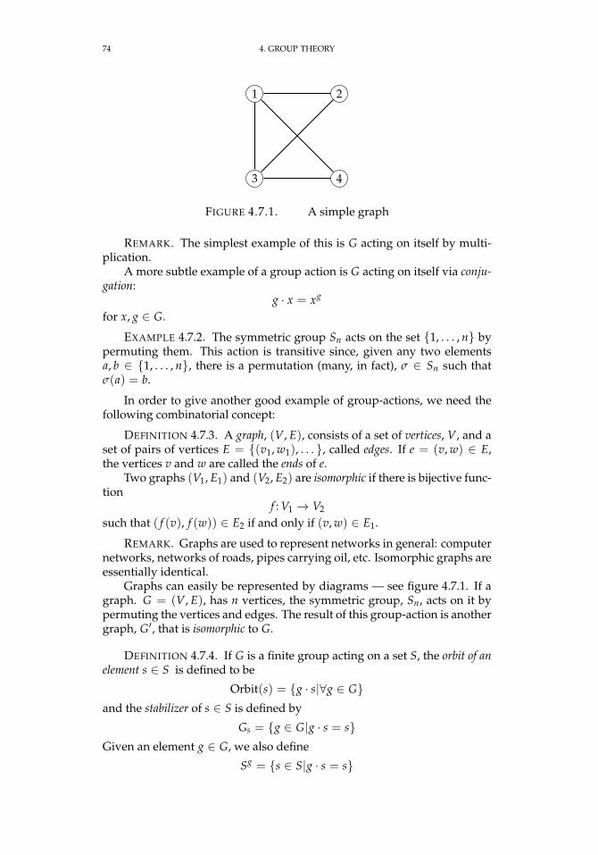
74 4. GROUP THEORY
1 2
3 4
FIGURE 4.7.1. A simple graph
REMARK. The simplest example of this is G acting on itself by multi-plication.
A more subtle example of a group action is G acting on itself via conju-gation:
g · x = xg
for x, g ∈ G.
EXAMPLE 4.7.2. The symmetric group Sn acts on the set 1, . . . , n bypermuting them. This action is transitive since, given any two elementsa, b ∈ 1, . . . , n, there is a permutation (many, in fact), σ ∈ Sn such thatσ(a) = b.
In order to give another good example of group-actions, we need thefollowing combinatorial concept:
DEFINITION 4.7.3. A graph, (V, E), consists of a set of vertices, V, and aset of pairs of vertices E = (v1, w1), . . . , called edges. If e = (v, w) ∈ E,the vertices v and w are called the ends of e.
Two graphs (V1, E1) and (V2, E2) are isomorphic if there is bijective func-tion
f : V1 → V2
such that ( f (v), f (w)) ∈ E2 if and only if (v, w) ∈ E1.
REMARK. Graphs are used to represent networks in general: computernetworks, networks of roads, pipes carrying oil, etc. Isomorphic graphs areessentially identical.
Graphs can easily be represented by diagrams — see figure 4.7.1. If agraph. G = (V, E), has n vertices, the symmetric group, Sn, acts on it bypermuting the vertices and edges. The result of this group-action is anothergraph, G′, that is isomorphic to G.
DEFINITION 4.7.4. If G is a finite group acting on a set S, the orbit of anelement s ∈ S is defined to be
Orbit(s) = g · s|∀g ∈ Gand the stabilizer of s ∈ S is defined by
Gs = g ∈ G|g · s = sGiven an element g ∈ G, we also define
Sg = s ∈ S|g · s = s
4.7. GROUP-ACTIONS 75
— the invariant set of g.The set of orbits is written as S/G.
REMARK. If T is the set of all possible graphs with n vertices, the sym-metric group Sn, acts on this by permuting vertices. The orbit of a graphwithin T is just the set of graphs isomorphic to it (even though the vertex-numbers that appear in its list of edges may vary).
The stabilizer of a graph consists of all permutations that leave all of thetwo-element subsets in E unchanged. If there are isolated vertices (i.e., ver-tices that are not endpoints of any edges), they can be permuted arbitrarilywithout changing the graph.
EXAMPLE 4.7.5. If H ⊂ G is a subgroup of a group, H acts on G byright-multiplication. The orbit of an element g ∈ G is just its coset gH. Thestabilizer of g ∈ G is the set of elements h ∈ H such that gh = g, i.e. just1 ∈ H.
PROPOSITION 4.7.6. If f : G× S→ S is a group-action on a set and s1, s2 ∈S are two elements such that
Orbit(s1) ∩Orbit(s2) 6= ∅
thenOrbit(s1) = Orbit(s2)
It follows that the group-action partitions S into a disjoint union of orbits
S =|S/G|⊔i=1
Orbit(si)
PROOF. If x ∈ Orbit(s1) ∩Orbit(s2), then
x = g1 · s1 = g2 · s2
for g1, g2 ∈ G. It follows that g−12 g1 · s1 = s2, so s2 ∈ Orbit(s1) and
Orbit(s2) ⊂ Orbit(s1). A similar argument shows that s1 ∈ Orbit(s2).
It is not hard to show that
PROPOSITION 4.7.7. If G acts on a set S and s ∈ S, then
|Orbit(s)| = [G: Gs] =|G||Gs|
or|Orbit(s)| · |Gs| = |G|
PROOF. We will show that there is a 1-1 correspondence between thecosets of Gs and elements of the orbit. If g1 · s = g2 · s then g−1
1 g2 · s = s sothat g−1
1 g2 ∈ Gs and g1Gs = g2Gs. On the other hand, if g1Gs 6= g2Gs, it isnot hard to see that g1 · s 6= g2 · s.
In many cases, we are most interested in the number of orbits of a group-action:
76 4. GROUP THEORY
LEMMA 4.7.8 (Burnside’s Lemma). If G is a finite group and S is a finiteset with group-action f : G× S→ S then
|S/G| = 1|G| ∑
g∈G|Sg|
REMARK. Although this result is called Burnside’s Lemma, it was notdue to him — he mentioned it in his 1897 book [23] and attributed it toFrobenius. It was also known to Cauchy, many years earlier. This is oftencited as an example of Stigler’s law of eponymy: “No scientific discoveryis named after its original discoverer.”
Sometimes it’s called “The Lemma not due to Burnside.”
William Burnside (1852 – 1927) was an English mathematician and re-searcher in the theory of finite groups. Burnside’s main area of researchwas in group representations. For many years Burnside’s classic, [23], wasthe standard text on group theory. One of Burnside’s best known contri-butions to group theory is his paqb theorem, which proves that every finitegroup whose order is divisible by fewer than three distinct primes is solv-able (see chapter 8 on page 295 for this concept). He also posed Burnside’sProblem (see 4.10.1 on page 87) in combinatorial group theory.
Baron Augustin-Louis Cauchy (1789 – 1857) was a French mathemati-cian, engineer and physicist who made pioneering contributions to severalbranches of mathematics, including: mathematical analysis and continuummechanics. He almost singlehandedly founded complex analysis and thestudy of permutation groups in abstract algebra.
PROOF. We begin by expressing a sum over elements of G as a sumover elements of S:
∑g∈G|Sg| = |(g, s) ∈ G× S|g · s = s| = ∑
s∈S|Gs|
Now we use proposition 4.7.7 on the previous page to conclude that |Gs| =|G|/|Orbit(s)| so we get
∑g∈G|Sg| = ∑
s∈S
|G||Orbit(s)| = |G| ·∑s∈S
1|Orbit(s)|
Since the group-action partitions S into disjoint orbits (see proposition 4.7.6on the preceding page), we can rewrite this as
(4.7.1) ∑g∈G|Sg| = |G| · ∑
z∈G/S
(∑s∈z
1|z|
)where z runs over all of the orbits in S. Now, simply note that, if z is an orbitof the G-action then
∑s∈z
1|z| = 1
4.7. GROUP-ACTIONS 77
so equation 4.7.1 on the preceding page becomes
∑g∈G|Sg| = |G| · ∑
z∈G/S1 = |G| · |G/S|
which proves the result.
EXAMPLE 4.7.9. Now we answer the question: how many distinct waysof coloring a square with five colors exist?
The colors are Red, Green, Yellow, Blue, and Orange and c(i) is thecolor of vertex i, where i = 1, . . . , 4. We regard two squares to be coloredthe same if one can be rotated or flipped so its colors coincide with those ofthe other square, i.e. the sets of colors are mapped into each other by theaction of D4 — see figure 4.1.1 on page 37.
(1) If g = 1 ∈ D4, then the invariant set consists of all possible colorson the 4 vertices, so |S1| = 54.
(2) If g = R ∈ D4, then a coloring is invariant under g if and onlyif all vertices are colored the same. It follows that |SR| = 5. Thesame is true for |SR3 | = 5.
(3) If g = R2, then vertex 1 must be the same color as vertex 3 andvertex 2 must be the same color as vertex 4. It follows that |SR2 | =52.
(4) If g = d1 ∈ D4, then vertex 1 must be the same color as vertex 3and no other conditions need be satisfied. It follows that |Sd1 | =53. A similar argument shows that |Sd2 | = 53.
(5) If g = c1 ∈ D4, then vertex 1 must be the same color as vertex 4and vertex 2 must be the same color as vertex 3. It follows that|Sc1 | = 52. A similar argument shows that |Sc2 | = 52.
Combining all of this together, we get that the number of distinct coloringsof the square are
18
(54 + 2 · 53 + 3 · 52 + 2 · 5
)= 120
EXAMPLE 4.7.10. Now we will apply Burnside’s Lemma to determin-ing the number of isomorphism classes of graphs with a bounded number ofvertices. Suppose we limit the number of vertices to 4. In this case, S is thenumber possible graphs on four vertices and the group acting on it is S4.
S1 = S and we can determine the size of this set by noting possibleedges involve pairs of vertices. There are (4
2) = 6 and each suchpair can either have an edge or not have one. This gives rise to26 = 64 possible graphs.
S4 has (42) = 6 two-cycles. If a graph is invariant under the two-
cycle (a, b) (with a < b taken from the set 1, 2, 3, 4) then verticesa and c are connected if and only if vertices b and c are connected.The possibilities are• a is connected to b or not: ×2• c is connected to d or not: ×2• a and b are both connected to c or not: ×2
78 4. GROUP THEORY
• a and b are both connected to d or not: ×2This gives rise to 24 = 16 possibilities.
S4 has 3 disjoint two-cycles (a, b)(c, d). The possibilities are:• a is connected to b or not: ×2• c is connected to d or not: ×2• a is connected to d and b is connected to c or not: ×2• a is connected to c and b is connected to d or not: ×2
Again, we get 24 = 16 possibilities. S4 has 8 three-cycles that look like (a, b, c). The possibilities are
• vertices a, b, c are all connected to each other or not: ×2• vertices a, b, c are all connected to vertex d or not: ×2
We get 4 possibilities. S4 has 6 cycles of length four (a, b, c, d) — the first entry is 1 and
the other three entries are permutations of 2, 3, 4 of which thereare 3! possibilities. The possibilities are:• a is connected to b which is connected to c which is connected
to d or not: ×2• each vertex is connected to the other 3 or not: ×2
We get 4 possibilities in this case.
The number of isomorphism classes of graphs with 4 vertices is, therefore,
1|S4| ∑
σ∈S4
|Sσ| = 124
(1 · 64 + 6 · 16 + 3 · 16 + 8 · 4 + 6 · 4) = 11
We conclude this section with development of the class equation.
PROPOSITION 4.7.11. If G is a group with element x, y the relation
x ∼ y
— called conjugation — if x = yg for some g ∈ G is an equivalence relation.
PROOF. Certainly x ∼ x because x = x1. If x ∼ y, x = yg it is not hardto see that y = xg−1
, so y ∼ x. If x ∼ y and y ∼ z then x = yg1 and y = zg2
so x = yg1g2 .
It follows that conjugation partitions G into a union of disjoint equiva-lence classes called conjugacy classes:
(4.7.2) G =⊔
Ci
Since the elements of Z(G) commute with everything in G, each of themis its own conjugacy class. We get an equation
(4.7.3) |G| = |Z(G)|+ |C1|+ · · ·+ |Ck|called the class equation of a group. Here C1, . . . , Ck are the various conju-gacy classes that contain more than one element.
Consider the action of G on itself via conjugation. The orbit of any el-ement g ∈ G is just its conjugacy class, say Ci as in equation 4.7.2. In thiscase, define
4.7. GROUP-ACTIONS 79
DEFINITION 4.7.12. If g ∈ G is an element of a group, we define thecentralizer of g, denoted ZG(g) — via
ZG(g) = x ∈ G|xg = gxREMARK. The centralizer of g is just the stabilizer of g in the group-
action via conjugation — i.e. ZG(g) = Gg.
COROLLARY 4.7.13. If g ∈ G is an element of a group G, the size of theconjugacy-class of g,
|Cg(G)| = [G: ZG(g)] = |G|/|ZG(g)|PROOF. This follows immediately from proposition 4.7.7 on page 75.
This implies that we can rewrite the class equation, 4.7.3 on the preced-ing page, as
(4.7.4) |G| = |Z(G)|+ [G: ZG(g1)] + · · ·+ [G: ZG(gk)]
where g1, . . . , gk ∈ G are representatives of the different conjugacy classes.This new version of the class equation has some interesting implications:
THEOREM 4.7.14 (Burnside’s Theorem for p-groups). If p is a primenumber and G is a group with |G| = pn for some integer n > 0 then |Z(G)| > 1and is a multiple of p.
PROOF. Each of the groups ZG(gi) is a subgroup of G so|ZG(gi)|
∣∣ |G| = pn. If |ZG(gi)| = |G|, then Z(G) = ZG(gi) = G and theresult follows.
If |ZG(gi)| < |G|, then |ZG(gi)| = pji for some ji > 0 and the classequation ( 4.7.4) becomes
pn = |Z(G)|+ pj1 + · · ·+ pjk
from which it follows that p∣∣ |Z(G)|.
DEFINITION 4.7.15. If G is a group with normal subgroup, N, and an-other subgroup, H, and a homomorphism
ϕ: H → Aut(N)
we define the semidirect product
G = N oϕ H
to have a set of elements N × H with group-operation defined by
(n1, h1) · (n2, h2) = (n1 ϕ(h1)(n2), h1h2)
REMARK. Note that G contains both N and H as subgroups and
N ∩ H = 1 ∈ G
This shows how lemma 4.6.13 on page 67 fails when the groups are notabelian.
In general, the semidirect product depends on the map
ϕ: H → Aut(N)
and different such maps give rise to non-isomorphic semidirect products.
80 4. GROUP THEORY
If ϕ: H → Aut(N) maps all of H to 1 ∈ Aut(N), then
N oϕ H = N ⊕ H
EXAMPLE 4.7.16. The dihedral group, D2n, satisfies
D2n ∼= Zn oϕ Z2
where 1 ∈ Z2 maps to the element of Aut(Zn) that sends each element toits additive inverse, giving rise to the familiar presentation
D2n =⟨
x, y|x2 = 1, yn = 1, xyx−1 = y−1⟩
EXERCISES.
1. If G is a group of order p2 for some prime p, show that G is abelian.
2. Verify that the semidirect product in definition 4.7.15 on the preced-ing page really defines a group.
3. What is the inverse of (n, h) ∈ N oϕ H?
4. In the semidirect product N oϕ H, show that conjugation of N by anelement h ∈ H, induces the automorphism ϕ(h).
5. If G is a group with subgroups N and H witha. N C G and abelianb. N ∩ H = 1c. G = NH.
Show thatG = N oϕ H
where ϕ: H → Aut(N) defined by conjugating N by elements of H.
4.8. The Sylow Theorems
4.8.1. Statement. These are deep theorems that are indispensable forclassifying finite groups — they form a partial converse to Lagrange’s The-orem ( 4.4.2 on page 43). For small values of n, in many cases, these threetheorems allow one to give an exhaustive list of all possible groups of ordern.
Peter Ludwig Mejdell Sylow (1832 – 1918) was a Norwegian mathematicianwho was a high school teacher from 1858 to 1898 and a substitute lecturer atChristiania University in 1862 — where he covered Galois theory. Duringthis time he posed a question that led to his celebrated Sylow Theorems,which he published in 1872.
Sylow’s first theorem is:

4.8. THE SYLOW THEOREMS 81
THEOREM 4.8.1 (First Sylow Theorem). If G is a group with |G| = pk ·m,where p is a prime number and gcd(p, m) = 1, then there exists a subgroupH ⊂ G with |H| = pk.
This subgroup, H, is called a Sylow p-subgroup of G.
THEOREM 4.8.2 (Second Sylow Theorem). Given G as above, all Sylowp-subgroups of G are conjugates of each other.
Sylow’s third theorem is
THEOREM 4.8.3 (Third Sylow Theorem). Given G as above, if np is thenumber of distinct Sylow p-subgroups, then np
∣∣m and np ≡ 1 (mod p).
EXAMPLE 4.8.4. In A4 we have Sylow subgroups of order 22 = 4 and 3.Consider subgroups of order 3: If n3 is the number of them, the third Sylowtheorem states that n3
∣∣ 4 and n3 ≡ 1 (mod 3). This means that n3 = 1 or 4.It turns out that A4 has four cyclic subgroups
〈(1, 2, 3)〉 , 〈(1, 2, 4)〉 , 〈(1, 3, 4)〉 , 〈(2, 3, 4)〉If we consider 2-Sylow subgroups, they must have order 22 = 4 and thenumber of them, n2 must satisfy n2
∣∣ 3 and n2 ≡ 1 (mod 2) — conditionsthat could be satisfied by n2 = 1 or 3. It turns out (and the Sylow theoremscannot tell us this) that n1 = 1 and the 2-Sylow subgroup is
〈(1, 2)(3, 4), (1, 4)(2, 3)〉4.8.2. Preliminary lemmas. In order to prove the Sylow Theorems, we
need several lemmas.
LEMMA 4.8.5. If H and K are subgroups of a finite group G, HK is generallyjust a set of elements. The size of this set is given by
(4.8.1) |HK| = |H| · |K||H ∩ K|REMARK. If H or K is a normal subgroup of G, then HK is a subgroup.
This result works even if neither H nor K are normal.
PROOF. Note that HK is a union of cosets
HK =⋃
h∈H
hK
Since each coset has |K| elements, it suffices to compute how many distinctcosets there are. Since h1K = h2K if and only if h−1
1 h2 ∈ K, it follows thath−1
1 h2 ∈ H ∩ K (since it is also in H). Lagrange’s theorem implies that thenumber of distinct such cosets is
|H||H ∩ K|
and since the size of these cosets is |K|, we get equation 4.8.1.
We will also need this somewhat odd lemma:
82 4. GROUP THEORY
LEMMA 4.8.6. If G is a finite group with p-Sylow subgroup P ⊂ G andQ ⊂ G is any other subgroup of order a power of p, then
Q ∩ NG(P) = Q ∩ P
REMARK. Recall that NG(P) is the normalizer of P — seedefinition 4.4.10 on page 46.
PROOF. Set H = Q ∩ NG(P). Since P C NG(P) it follows that Q ∩ P CH. Since H ⊂ Q, the statement of the lemma is equivalent to H ⊂ P. SinceH ⊂ NG(P) and P C NG(P), it follows that HP is a subgroup of NG(P) —and also a subgroup of G. Lemma 4.8.5 on the preceding page implies that
|HP| = |H| · |P||H ∩ P|Since all of the numbers in this quotient are powers of p, it follows that HPis a p-group containing P. Since P is the maximal such p-group, it followsthat HP = P, which implies that H ⊂ P.
4.8.3. Proof of the Sylow theorems. We begin with theorem 4.8.1 onthe previous page — the statement that Sylow subgroups exist. It is triv-ially true if |G| = 1 so we will do induction on |G|. If |G| = pk · m withgcd(p, m) = 1, we consider two cases:
Case 1: p∣∣ |Z(G)| In this case, we know that Z(G) has a subgroup, H,
of order p (see theorem 4.6.10 on page 65 and proposition 4.3.4 on page 41)which — since it is in the center — is normal. Form the quotient
GH
= G′
By the inductive hypothesis, G′ has a Sylow p subgroup, S, of order pk−1.The Correspondence Theorem (see exercise 5 on page 48) implies that Ghas a subgroup of order pk.
Case 2: p - |Z(G)|. In this case, we write out the class equation (seeequation 4.7.4 on page 79):
|G| = |Z(G)|+ [G: ZG(g1)] + · · ·+ [G: ZG(gn)]
If p∣∣ [G: C(gi)] for all i, then |Z(G)| is a linear combination of multiples of
p so p| |Z(G)|. Since we are assuming that this is not true, we concludethat p - [G: ZG(gi)] for at least one value of i. If |ZG(gi)| = pj · `, withgcd(p, `) = 1 we get
[G: ZG(gi)] =|G|
|ZG(gi)|= pk−j · m
`
and since p - [G: ZG(gi)], we have k = j. Since |ZG(gi)| < |G| inductionimplies that ZG(gi) has a subgroup of order pk — which is also a Sylowp-subgroup of G.
Now we prove theorem 4.8.3 on the preceding page and 4.8.2 on theprevious page. Let S be a Sylow p-subgroup of G (which we now knowexists) and let
Z = S1, . . . , Sr
4.8. THE SYLOW THEOREMS 83
be the set of all conjugates of S. In addition, let T be a p-subgroup of G andlet
Z = Orbit1 ∪ · · · ∪Orbits
where Orbiti are the orbits (see definition 4.7.4 on page 74) of the action ofT on the Sj by conjugation — so that
r = |Orbit1 |+ · · ·+ |Orbits |and renumber the elements of Z so that the first s terms are representativesof distinct orbits of T. It follows from lemma 4.7.7 on page 75 that
|Orbiti | = [T: NT(Si)]
By definition, NT(Si) = NG(Si) ∩ T, so lemma 4.8.6 on the facing pageimplies that NT(Si) = Si ∩ T and we get
|Orbiti | = [T: T ∩ Si]
Since T was an arbitrary p-subgroup of G, we can set T = S1 and
|Orbit1 | = 1
Since S1 6= Si for i > 1, we get |S1 ∩ Si| < |S1| if i > 1, which implies that
|Orbiti | = [S1: S1 ∩ Si] > 1
for i > 1. Since S1 and Si are p-groups, we conclude that p∣∣ [S1: S1 ∩ Si] and
|Orbiti | for i > 1.We conclude that
r = |Orbit1 |+ (|Orbit2 |+ · · ·+ |Orbits |) ≡ 1 (mod p)
Now we are in a position to prove that all Sylow subgroups are conju-gates of each other. Suppose T is a p-subgroup of G that is not contained inany of the Si. Then the argument used above implies that
|Orbiti | = [T: T ∩ Si] > 1
for all i — and p divides it. This implies that p∣∣ r, which contradicts the fact
that r ≡ 1 (mod p).It follows that all p-subgroups are contained in conjugates of this one
Sylow subgroup. Since they have the same number of elements, all Sylowsubgroups must be on this list of conjugates of one Sylow subgroup.
The final statement to be proved is that r∣∣m:
Since r is the size of the orbit of S under the action of G, lemma 4.7.7 onpage 75 implies that
r = [G: GS]
where GS is the stabilizer of S — see definition 4.7.4 on page 74 — but thisis identical to the definition of the normalizer of S, so
r = [G: NG(S)] =|G|
|NG(S)|Since S ⊂ NG(S), we have |NG(S)| = pk · ` and
r =pk ·mpk · ` =
m`
or r · ` = m and r∣∣m.
84 4. GROUP THEORY
EXERCISES.
1. Show that every group of order 35 is cyclic.
2. Show that no group of order 70 can be simple.
4.9. Subnormal series
We can break groups into smaller factors in various ways.
DEFINITION 4.9.1. If G is a group, a subnormal series
1 ⊂ G0 ⊂ G1 ⊂ · · · ⊂ G
is a sequence of subgroups of G such that Gi C Gi+1 for all i.
REMARK. Note that Gi C Gi+1 but this does not mean Gi C G.Since each term is a normal subgroup of the next, the quotients
Gi+1
Gi
are well-defined for all i.
Now we will discuss certain standard classes of subnormal series.
DEFINITION 4.9.2. If G is a group, its derived series
· · · ⊂ Gn ⊂ · · · ⊂ G1 ⊂ G0 = G
is defined byGn+1 = [Gn, Gn]
REMARK. Note that all of the quotients Gn/Gn+1 are abelian.Derived series do not necessarily terminate in a finite number of steps:
Since An is simple for n ≥ 5 (see theorem 4.5.15) and [An, An] C An itfollows that all of the terms of the derived series for An are equal to An.
The next class of subnormal series is particularly important in the clas-sification of finite groups.
DEFINITION 4.9.3. If G is a finite group, its composition series is a sub-normal series
1 ⊂ G0 C G1 C · · · C Gk C G
with the property that each quotient
Gi+1
Gi= Fi
is a simple group. The quotients, Fi, are called composition factors.
4.9. SUBNORMAL SERIES 85
REMARK. In a manner of speaking, we are fracturing G into a series ofsmaller groups — the composition factors. Each of them fits into what iscalled a group-extension
1→ Gi → Gi+1 → Fi → 1
With suitable information, it is possible to reconstruct Gi+1 from Gi and Fi— see chapter 13 on page 429 and section 13.3.2 on page 454.
This is related to the Isomorphism Problem for finite groups:List all isomorphism classes of finite groups.
Since it is possible to construct groups from normal subgroups and quo-tients, this follows (to some extent) from the corresponding problem forsimple groups:
List all isomorphism classes of finite simple groups.Since this problem has been solved, in principle, so has the former. In 1983,Daniel Gorenstein announced that finite simple groups had been classified,but his classification turned out to be incomplete.
The first complete classification was published in 2004 by Aschbacherand Smith. At 1221 pages, their proof is beyond the scope of the presenttext. See the survey [4].
LEMMA 4.9.4. If G is a finite group, a composition series for G exists.
PROOF. Let1 ⊂ G0 C G1 C · · · C Gk C G
be a subnormal series of maximal length (i.e., maximal value of k). We claimthat
Gi+1
Gi= Fi
is simple for all i. If not, let A C Fi be a proper normal subgroup. If
pi: Gi+1 → Fi
is the standard projection, then p−1i (A) C Gi+1 (see exercise 5 on page 48)
and Gi C p−1i (A) so we get a subnormal series
1 ⊂ G0 C G1 C · · · C Gi C p−1i (A) C Gi+1 C · · · C Gk C G
of length k + 1, a contradiction.
In an analogy to the unique factorization of integers into primes, a groupuniquely determines its composition factors.
THEOREM 4.9.5 (Jordan-Hölder). If G is a finite group and
1 ⊂ G0 C G1 C · · · C Gk C Gand
1 ⊂ H0 C H1 C · · · C H` C Gare two composition series for G, then k = ` and both series have the same compo-sition factors — possibly occurring in a different order.
86 4. GROUP THEORY
PROOF. The statement that k = ` follows quickly from lemma 4.9.4 onthe preceding page: its proof implies that a subnormal series is a composi-tion series if and only if it is of maximal length.
We prove the rest of the theorem by induction on |G|. It’s trivial if|G| = 1.
Suppose |G| = n and the theorem is true for all groups of order < n. IfGk = Hk, we apply the inductive hypothesis to conclude that the theoremis true for Gk which implies it is true for G.
Consequently, assume Gk 6= Hk and let K = Gk ∩ Hk.Note that K C Hk (see exercise 3 on page 47) and
(4.9.1)HkK∼= Gk · Hk
Gk
(see exercise 4 on page 48) where Gk · Hk ⊂ G is a normal subgroup (seeexercise 1 on page 47). Note that
Gk · Hk/Gk C G/Gk
Since the latter group is simple, we must have Gk · Hk/Gk = G/Gk so that:(1) G = Gk · Hk(2) Gk · Hk/Gk and Hk/K are also simple (by equation 4.9.1).
It follows that we can get a composition series for Hk via
1 C K0 C · · · C Kt C K C Hk
where1 C K0 C · · · C Kt C K
is a composition series for K, and t + 1 = k− 1, and induction implies that
K1/K0, . . . , Kt/Kt−1, Hk/K = H1/H0, . . . , Hk/Hk−1as sets of isomorphism classes of groups. Furthermore,
1 C K0 C · · · C Kt C K C Gk
is a composition series for Gk and we have
K1/K0, . . . , Kt/Kt−1, Gk/K = G1/G0, . . . , Gk/Gk−1It follows that
H1/H0, . . . , Hk/Hk−1 = G1/G0, . . . , Gk/Gk−1and the conclusion follows from G/Gk
∼= Hk and G/Hk∼= Gk (since G =
Gk · Hk).
EXAMPLE 4.9.6. If G is abelian, all of its composition factors are of theform Zpi , for pi all primes, since these are the simple abelian groups.
In our later work on Galois Theory (see chapter 8 on page 295) we willneed a class of groups that have this property in common with abeliangroups:
DEFINITION 4.9.7. A finite group, G, is defined to be solvable if its com-position factors are all of the form Zpi for primes pi. The primes that occurin the manner are called the associated primes of G.
4.10. FREE GROUPS 87
Not all solvable groups are abelian. For instance S3 has a normal sub-group generated by (1, 2, 3) that is isomorphic to Z3 and S3/Z3 ∼= Z2.
EXAMPLE 4.9.8. On the other hand, the groups Sn for n ≥ 5 are notsolvable: their composition factors are Z2 and An, which are known tobe simple (see theorem 4.5.15). Theorem 4.9.5 on page 85 implies that allcomposition series for Sn will have these factors.
EXERCISES.
1. If G is a solvable group, show that it contains a normal subgroup Hsuch that [G: H] is a prime number.
2. Show that we could’ve defined solvable groups as groups with asubnormal series whose quotients are abelian.
3. If G is a finite group, show that its derived series becomes constantat some point.
4. Show that a finite group, G, is solvable if and only if its derivedseries terminates after a finite number of steps, i.e. if its derived series
· · · ⊂ Gn ⊂ · · · ⊂ G1 ⊂ G0 = G
has the property that there exists an integer k such that Gi = 1 for i ≥ k.
5. Show that quotients and subgroups of solvable groups are solvable.
6. Let G be a group with a normal subgroup H. If H and G/H are bothsolvable, show that G must also be solvable.
4.10. Free Groups
4.10.1. Introduction. In this section, we will introduce groups that are“free-er” than the free abelian groups defined in section 4.6 on page 58.They can be used to define presentations of groups — ways of describingthem using “coordinates” and “equations”. This gives rise to an area ofgroup theory called combinatorial group theory.
Combinatorial group theory originally arose in algebraic topology,with the study of knot-groups. One of the first purely group-theoreticproblems in the field was
PROBLEM 4.10.1 (Burnside’s Problem). If n > 1 is an integer and G is afinitely generated group that satisfies the equation
xn = 1
for all x ∈ G, is G finite?
88 4. GROUP THEORY
Burnside showed that the answer was “yes” for n = 2, 3, 4, 6. Thebreakthrough in Burnside’s problem was achieved by Pyotr Novikov andSergei Adian in 1968 (see [6]). Using a combinatorial argument, theyshowed that for every odd number n with n > 4381, there exist infinite,finitely generated groups where every element satisfies xn = 1.
DEFINITION 4.10.2. If X = x1, . . . is a set of symbols, the free groupon X, FX consists of equivalence classes of all possible finite strings
xα1i1· · · xαn
in
where the xi ∈ X, the αi ∈ Z, and the product of two such strings is theirconcatenation. Two strings are equivalent or freely equal if one can be trans-formed into the other via the following operations or their inverses:Identity: 1 is equivalent to the empty string,Consolidation: whenever we have · · · xα
j · xβj · · · in a string, we may re-
place it by · · · xα+βj · · · to get an equivalent string,
Culling: whenever a factor in a string has exponent 0, we may remove it.
REMARK. Sometimes, we’ll abuse the terminology and say things like“These strings are freely equal as elements of the free group, FX”. This isabuse because the elements of FX are equivalence classes of strings, wherestrings are equivalent if they’re freely equal.”
Deciding when two strings are equivalent is fairly easy:
DEFINITION 4.10.3. If xα1i1· · · xαn
in ∈ FX is a string in a free group, thereduced form of xα1
i1· · · xαn
in is the result of applying the operations in defini-tion 4.10.2 as many times as possible to minimize the number of factors inxα1
i1· · · xαn
in .
REMARK. A string, xα1i1· · · xαn
in , is reduced if and only if
(1) xij 6= xij+1 for all j, and(2) αi 6= 0 for all i
Since reduced forms of words are unique and equivalent to the originalwords, we have
PROPOSITION 4.10.4. Two words w1, w2 ∈ FX are equivalent if and only iftheir reduced forms are equal.
Note that the inverse of xα1i1· · · xαn
in is x−αnin · · · x−α1
i1— we must negate
the exponents and reverse the order of the factors.Also notice that the relations that words satisfy (in definition 4.10.2)
are relations that all elements in all groups must satisfy. This has severalconsequences:
THEOREM 4.10.5. Let FX be a free group on a set of generators, X, and let Gbe a group. Any function
f : X → Gextends uniquely to a group-homomorphism
f : FX → G
4.10. FREE GROUPS 89
REMARK. This can be regarded as the defining property of a free group.
PROOF. Simply define
f (xα1i1· · · xαn
in ) = f (xi1)α1 · · · f (xin)
αn
This immediately implies:
PROPOSITION 4.10.6. If G is any group, there exists a free group FX and asurjective homomorphism
f : FX → G
If G is finitely generated, then X can be finite.
REMARK. Compare this to proposition 4.6.7 on page 62. Just as everyabelian group is a quotient of a free abelian group, every group (includingabelian groups) is a quotient of a free group.
PROOF. Let FX be a free group on the set, X.If G is finitely generated,then the elements of X are in a 1-1 correspondence with its generators. Oth-erwise it is in a 1-1 correspondence with the non-identity elements of G, soxi 7→ gi and define f by
f (xα1i1· · · xαn
in ) = gα1i1· · · gαn
in ∈ G
4.10.2. Combinatorial group theory. This leads to the topic of presen-tations of groups:
DEFINITION 4.10.7. If X = x1, . . . is a set of symbols andR = r1, . . . is a set of elements of FX the symbol, called a presentation of agroup, G,,
(4.10.1) 〈X|R〉is an isomorphism
G =FX
〈R〉FX
where 〈R〉 ⊂ FX is the subgroup generated by the elements of R and 〈R〉FX
is the normal closure of this subgroup — see definition 4.4.11 on page 46.The elements of X are called the generators of G and the elements of R arecalled the relators or relations of G.
REMARK. The group being presented is G, which is generated by im-ages of the xi under the projection
FX →FX
〈R〉FX
and the ri = 1 are “equations” that these images satisfy.
90 4. GROUP THEORY
For instanceZn = 〈x|xn〉
is a presentation of Zn.Sometimes we write the relators as equations, so
Z⊕Z = 〈x, y|xy = yx〉 =⟨
x, y|xyx−1y−1⟩
are presentations. When a relation is not written as an equation, it is as-sumed to equal 1.
Proposition 4.5.17 on page 57 shows that
(4.10.2) D2n =⟨
x, y|xn, yxy = x−1⟩
is a presentation of the dihedral group.A given group can have many different presentations that may not re-
semble each other. For instance, it turns out that
S3 =⟨
a, b|a3, b2, ab = ba2⟩=⟨
x, y|x2, y2, (xy)3⟩
This leads to Max Dehn’s three fundamental problems in combinatorialgroup theory:
Given a presentation of a group G like that in equation 4.10.1 on theprevious page, we have
(1) The word problem: Determine whether a word in the generators,like xα1
i1· · · xαn
in , is the identity element in a finite number of steps.(2) The conjugacy problem: Given two words in the generators, de-
termine whether they represent conjugate elements of G in a finitenumber of steps.
(3) The isomorphism problem: Given two group-presentations, in a fi-nite number of steps determine whether they represent isomor-phic groups.
If a free group has the standard presentation, 〈X| 〉, proposition 4.10.4 onpage 88 solves the word problem: a word is the identity element if andonly if its reduced form is empty.
Notice that these problems refer to presentations of groups, not thegroups themselves. Solutions to, say, the word problem will be verydifferent for different presentations of a group.
Max Dehn (1878 – 1952) was a German-born American mathematician andstudent of David Hilbert. His most famous work was in the fields of geom-etry, topology, and geometric group theory. He is also known for being thefirst to resolve one of Hilbert’s famous 23 problems. Dehn solved Hilbert’sthird problem:
Given two polyhedra of equal volume, is it possible tocut the first into finitely many pieces that can be reassem-bled to give the second?
Dehn produced a counterexample.
If our group is the dihedral group with presentation
(4.10.3) D2n =⟨
x, y|xn, y2, yxy = x−1⟩
4.10. FREE GROUPS 91
proposition 4.5.17 on page 57 shows that the word-problem can be solvedvia
Given a string of x’s and y’s, repeat the following two operations untilthe string is of the form xiyj
reduce all exponents of x modulo n and all exponents of y modulo2.
replace each occurrence of yx by x−1y = xn−1yThe string represents the identity element if and only if, at the end, i = j =0.
This is the solution of the word problem for the presentation in equa-tion 4.10.3 on the facing page of the dihedral group.
In 1955, Novikov (see [85]) showed that there are finitegroup-presentations whose word problems are unsolvable. In 1958, Boone(see [15]) gave examples of such presentations with 2 generators and 32relations.
Given a presentation for a group
G = 〈X|R〉Tietze showed that it is possible to get any other presentation for G usingthe Tietze transformations
DEFINITION 4.10.8. The Tietze transformations are:T1: If words w1, . . . , wk are derivable from the relators in R (i.e. they are
products of conjugates of the ri ∈ R), they can be added to R.T2: If some of the relators ri1 , . . . , rik are derivable from the others, they may
be deleted from R.T3: If w1, . . . , wm are words in the symbols in X, we may add generators
y1, . . . , ym to X if we also add relations yi = wi to R.T4: If we have a relation xi = w, where w is a word in X \ xi, we may
delete the relation from R and the symbol xi from X. We mustalso replace every occurrence of xi in the remaining relations byw.
REMARK. The even numbered transformations are the inverses of theodd-numbered ones. Some authors list only two transformations.
THEOREM 4.10.9. Tietze transformations replace one presentation of a groupby another. If a group has two different presentations
G =⟨xi |
rj⟩
(4.10.4)
= 〈yk | s`〉one can be transformed into the other by Tietze transformations.
REMARK. This does not solve the isomorphism problem. It gives noalgorithm for finding a sequence of Tietze transformations to go from onepresentation to another.
PROOF. It is not hard to see these transformations preserve the group,G. T1 asserts relations already known to be true in G, and T2 deletes them.
92 4. GROUP THEORY
T3 adds new elements to G and equates them to elements already present,and T4 deletes them.
Given the two presentations for G in equation 4.10.4 on the previouspage, we have surjections
f : FX → Gg: FY → G
where X = xi and Y = yk. We start with presentation⟨xi |
rj⟩
.Let ui ∈ FX have the property that f (ui) = g(yi). Then applications of T3convert the presentation to
G =⟨xi ,
yj|
rj
,
yj = uj⟩
If we plug the uj into the relations, s`and map them via f we get
f (s`(u1, . . . , um)) = s`( f (u1), . . . , f (um))
= s`(g(y1), . . . , g(ym))
= g (s`(y1, . . . , ym))
= 1
which means that s`(u1, . . . , um) follows from the set of relations
rj
. Therelations
yj = uj
imply that s`(y1, . . . , ym) follows from the relations
rj∪
yj = uj
. We can, consequently use T1 multiple times to getanother presentation of G:
G =⟨xi ,
yj|
rj
,
yj = uj
, s`⟩
with mapf ∪ g: FX∪Y → G
Now let vi ∈ FY have the property that g(vi) = f (xi). Since g(vi) = f (xi),the words vix−1
i map to 1 ∈ G under this new map, so that vix−1i are con-
sequences of the relations
rj∪
yj = uj
. We can use T1 to add them tothe relations, getting
G =⟨xi ,
yj|
rj
,
yj = uj
, s` , vi = xi⟩
Now we can use T4 several times to delete the x’s from the generators
G =⟨
yj|
rj(vi)
,
yj = uj
, s`⟩
where the rj(vi) are relators with the variables xi replaced by the words vithat are written in the yj. Note that
g(rj(vi)) = rj(g(vi))
= rj( f (xi))
= f(rj(xi)
)= 1
so that the rj(vi) are implied by the relators, s`. We can use T2 to deletethem and get the presentation
G =⟨
yj| s`
⟩
4.10. FREE GROUPS 93
EXAMPLE 4.10.10. Suppose we start with the presentation
〈a, b|aba = bab〉Now we introduce new generators x = ab, and y = aba. Two applicationsof T3 give
〈a, b, x, y|aba = bab, x = ab, y = aba〉Now x−1y = a, so we can eliminate a using T4 to get⟨
b, x, y|x−1ybx−1y = bx−1yb, x = x−1yb, y = x−1ybx−1y⟩
or ⟨b, x, y|x−1ybx−1y = bx−1yb, x2 = yb, 1 = x−1ybx−1
⟩or ⟨
b, x, y|x−1ybx−1y = bx−1yb, x2 = yb, x2 = yb⟩
We use T2 to eliminate the last relation and note that b = y−1x2. Apply T4again to eliminate b and get⟨
b, x, y|x−1yy−1x2x−1y = y−1x2x−1yy−1x2, x2 = yy−1x2⟩
or ⟨x, y|y = y−1x3, x2 = x2
⟩or ⟨
x, y|y2 = x3, x2 = x2⟩
and we use T2 to eliminate the last relation to get⟨x, y|y2 = x3
⟩This is a very different-appearing presentation for the same group.
EXERCISES.
1. Let G be a group with normal subgroup A C G and quotient
F =GA
a free group. Show that G = A oα F, where α: F → Aut(A) is defined byconjugation.
2. Show that
G =⟨
xn, n ∈ Z+|xnn = xn−1, n ∈ 2, . . .
⟩is a presentation for (Q,+), the rational numbers under addition.
94 4. GROUP THEORY
3. Show, using Tietze transformations, that⟨a, b, c|b(abc−1)2a, c(abc−1)3
⟩is the free group on two generators.
Hint: In Fx,y adjoin the new generators a = xy, b = y−1x, and c = x3.Then solve for x and y in terms of a, b, c.
4. Show that the Prüfer group (see example 4.1.10 on page 38), Z/p∞,can be presented as
Z/p∞ =⟨
x1, x2, x3, . . . |xp1 = 1, xp
2 = x1, xp3 = x2, . . .
⟩
4.10.3. Quotients and subgroups. Given a group-presentation
G = 〈X|R〉let H be a normal subgroup generated by the conjugates of element g1, . . . , gn ∈ G.If we find words w1, . . . , wn in FX representing these elements, we get a presentationof G/H:
G/S = 〈X|R, w1, . . . , wn〉This follows immediately from the fact that a group-presentation defines a quotientof a free group.
A related but harder (and more interesting!) problem is how we can get apresentation of a subgroup of G.
We begin with
DEFINITION 4.10.11. If H ⊂ G = 〈X|R〉 is a subgroup generated by wordsw1, . . . , wk ∈ FX , a rewriting process for H with respect to the words wi is a function
ξ: U → V
where U is the set of words of FX that define elements of H and V = FS, wheresw1 , . . . , swk are symbols in a one-to-one correspondence with the wi. If w ∈ FXdefines an element of H, we require that
ξ(w)sw1→w1,....swk→wk
defines the same element of H as w. Here ξ(w)sw1→w1,....swk→wk denotes the result oftaking the word ξ(w) ∈ FS — a word in the sj — and substituting wi for swi for alli, obtaining a word in FX .
REMARK. In other words, ξ simply rewrites a word representing an elementof H into one in the generators of H.
Here’s an example:
EXAMPLE 4.10.12. LetG = 〈x, y| 〉
and let H be the normal subgroup generated by y and its conjugates. This means His generated by elements
sk = xkyx−k
4.10. FREE GROUPS 95
Note that
s`k = xkyx−k · · · xkyx−k︸ ︷︷ ︸` times
= xky`x−k
Ifw = xα1 yβ1 · · · xαt yβt
is a word witht
∑i=1
αi = 0
we can rewrite it as
w =(
xα1 yx−α1)β1 ·
(xα1+α2 yx−α1−α2
)β2 · · ·(
xα1+···+αt yx−α1−···−αt)βt(4.10.5)
= sβ1α1 · · · s
βtα1+···+αt
so that w ∈ H and equation 4.10.5 constitutes a rewriting process for H with respectto the generators S = sj, i.e.
ξ(w) = sβ1α1 · · · s
βtα1+···+αt
The idea of finding a presentation for H is fairly simple:
Since the relators in the presentation of G represent its identityelement, they represent an element of H as well, so rewrite therelators of G using the rewriting process and we’re done!
Unfortunately, “the devil’s in the details”. Handling them gives us a (rather useless)presentation for H:
THEOREM 4.10.13. If
(4.10.6) G = 〈X|R〉is a presentation of a group, H = 〈g1, . . . , gn〉 is a subgroup, where gi is represented by aword wi ∈ FX , and
ξ: 〈w1, . . . , wn〉 → FS
is a rewriting process for H with respect to the wi, then the following is a presentationfor H:
generators S = s1, . . . , sn in a one-to-one correspondence with the wordsw1, . . . .wn,
relations(1) si = ξ(wi) for all i.(2) ξ(w) = ξ(w′) for all pairs w, w′ of words representing elements of H that
are freely equal6 in FX ,(3) ξ(u · v) = ξ(u) · ξ(v) for all pairs of words u, v representing elements of
H,(4) ξ(w · r · w−1) = 1 where w runs over all words in FX and r runs over all
defining relations, R, in equation 4.10.6.
REMARK. Note that this presentation for H usually has an infinite number ofrelations! We will work at simplifying it.
6See definition 4.10.2 on page 88, for the definition of ‘freely equal.’
96 4. GROUP THEORY
PROOF. The statement about generators is clear. It is also not hard to see thatthe stated relations are reasonable — i.e., they are valid in H. For instance, in state-ment 1 on the preceding page, si and wi and ξ(wi) represent the same element of Hso it is valid to equate them.
If two words are freely equal in FX , they represent the same element of G,therefore also of H and statement 2 on the previous page makes sense. Statements 3on the preceding page and 4 on the previous page are also clear.
The hard part of this proof is showing that all relations in H can be derivedfrom these.
We begin by deriving some consequences of the four sets of relations in 1 onthe preceding page through 4 on the previous page:
Statement 3 on the preceding page implies that ξ(1) · ξ(1) = ξ(1) or ξ(1) = 1.If we set v = u−1, we get
ξ(u) · ξ(u−1) = ξ(1) = 1
so that ξ(u−1) = ξ(u)−1.A simple induction shows that, if b1, . . . , bk ∈ FX are words representing ele-
ments of H, then
(4.10.7) ξ(bα11 · · · b
αkk ) = ξ(b1)
α1 · · · ξ(bk)αk
and this is a direct consequence of statements 2 on the previous page and 3 on thepreceding page.
Suppose
sα11 · · · sαr
r
is a word in FS that maps to 1 in H — i.e., is a relator in presentation of H. We willshow that
sα11 · · · sαr
r = 1
is a consequence of statements 1 on the previous page through 4 on the precedingpage. Let qi ∈ FX be a word representing si for all i. Then statement 1 on theprevious page and equation 4.10.7 imply that
sα11 · · · sαr
r = ξ(q1)α1 · · · ξ(qr)
αr = ξ(qα11 · · · qαr
r )
Since qα11 · · · q
αrr ∈ FX maps to 1 in G, it is in the normal closure of the relations of G,
namely the elements of R. It follows that qα11 · · · q
αrr is freely equal to
ry11 · · · r
y``
where the ri ∈ R and the yi ∈ FX are some words. We conclude that
sα11 · · · sαr
r = ξ(q1)α1 · · · ξ(qr)
αr
= ξ(qα11 · · · qαr
r )
= ξ(ry11 · · · r
y`` )
= ξ(ry11 ) · · · ξ(ry`
` ) = 1 · · · 1 = 1
so that sα11 · · · s
αrr = 1 is a consequence of statements 1 through 4 on the previous
page.
We will explore alternate rewriting processes that automatically satisfy manyof the conditions in theorem 4.10.13 on the preceding page, resulting in a simplerpresentation.
4.10. FREE GROUPS 97
DEFINITION 4.10.14. If
G = 〈X|R〉is a presentation of a group and H is a subgroup let
C = 1, e(g1), . . .
be a set of distinct right coset-representatives — i.e. for each coset Hg, we select asingle element e(g) ∈ Hg, to represent it. For the coset of 1, namely H, we select theelement 1.
A right coset representative function is a mapping
η: FX → FX
defined as follows:If w represents the element g ∈ G, η(w) ∈ FX is a word representing the chosen
representative for the coset Hg, namely e(g).The notation Cη = 1, w1, . . . denotes the set of words representing the coset
representatives, so |Cη | = [G: H].
REMARK. Several arbitrary choices were made in defining η:
(1) the elements g selected to represent a coset Hg(2) the words, η(∗), selected to represent these elements in FX
Another common term for a coset representative function is transversal.In general, we want to pick words that are as short and simple as possible.
EXAMPLE 4.10.15. We return to the group and subgroup in example 4.10.12on page 94. Since H is a normal subgroup, the cosets of H in G are in a 1-1 cor-respondence with elements of G/H = 〈x| 〉 = Z. For the coset Hxk, we pick therepresentative xk — and we also pick this word in Fx,y so our coset representativefunction is
η(xα1 yβ1 · · · xαn yβn ) = x∑ni=1 αi
In this case Cη = xn, ∀n ∈ Z.
LEMMA 4.10.16. Under the conditions of definition 4.10.14,
(1) If w ∈ H, then
(4.10.8) η(w) = 1
(2) If v, w ∈ FX are freely equal, then η(v) = η(w),(3) If w ∈ FX , then η(η(w)) = η(w)(4) If v, w ∈ FX , then η(vw) = η(η(v)w)(5)
(4.10.9)(
k′xη(k′x)−1)−1
= kx−1η(
kx−1)−1
where k ∈ Cη , x ∈ X, and k′ = η(kx−1).
REMARK. If we write
tk,xε = kxεη(kxε)−1
with ε = ±1, then equation 4 implies that
(4.10.10) tk,x−1 = t−1η(kx−1),x
98 4. GROUP THEORY
PROOF. Most of these are immediate from definition 4.10.14 on the precedingpage. To show the final statement, set k′ = η(kx−1). Then
(k′xη(k′x)−1
)·(
kx−1η(
kx−1)−1
)= η(kx−1)xη(η(kx−1)x)−1
· kx−1η(
kx−1)−1
= η(kx−1)xη(kx−1x)−1
· kx−1η(
kx−1)−1
=(
η(kx−1)xη(k)−1)·(
kx−1η(
kx−1)−1
)=(
η(kx−1)xk−1)·(
kx−1η(
kx−1)−1
)= η(kx−1)x · x−1 · η
(kx−1
)−1
= 1
Given a coset representative function, we can define a rewriting process thatautomatically satisfies some of the conditions in theorem 4.10.13 on page 95 — so wecan simplify the relations in the presentation.
If G = 〈X|R〉 is a presentation of a group and H is a subgroup with a cosetrepresentative function η: FX → FX , consider elements of the form
kixjη(kixj)−1
where ki ∈ Cηand xj ∈ X. This is an element of H since η(kixk) is in the sameright-coset as kixj.
THEOREM 4.10.17. If G = 〈X|R〉 is a presentation of a group and H is a subgroupwith a coset representative function η: FX → FX , define words
(4.10.11) tk,xε = kxεη(kixε)−1
where k runs over the elements of Cη and xj runs over X. These words generate H. In fact,if
xα11 · · · xαn
n
is a word representing an element of H with all exponents equal to ±17, then
(4.10.12) xα11 · · · xαn
n =(
t1,xα11
)·(
tη(xα11 ),xα2
2
)· · ·(
tη(xα1
1 ···xαn−1n−1 ),xαn
n
)REMARK. This first appeared in [93], in connection with algebraic topology
(knot theory).
7So x3 is written as xxx, and x−2 as x−1x−1.
4.10. FREE GROUPS 99
PROOF. Just fill in what the t-symbols equal (from equation 4.10.11 on the fac-ing page):
t1.xα11
= xα11 η(xα1
1 )−1
tη(xα11 ),xα2
2= η(xα1
1 )xα22 η(η(xα1
1 )xα22 )−1
= η(xα11 )xα2
2 · η(xα11 xα2
2 )−1 by lemma 4.10.16 on page 97
tη(xα11 xα2
2 ),xα33
= η(xα11 xα2
2 )xα33 · η(xα1
1 xα22 xα3
3 )−1
...
tη(xα1
1 ···xαn−1n−1 ),xαn
n= η(xα1
1 · · · xαn−1n−1 )xαn
n η(xα11 · · · x
αn−1n−1 xαn
n )−1
= η(xα11 · · · x
αn−1n−1 )xαn
n
because η(xα11 · · · x
αn−1n−1 xαn
n ) = 1
since xα11 · · · x
αn−1n−1 xαn
n ∈ H
We get a telescoping product in which all of the η(∗)-factors cancel, and we are leftwith our original word,
xα11 · · · xαn
n
Kurt Werner Friedrich Reidemeister (1893 – 1971) was a mathematicianborn in Braunschweig (Brunswick), Germany. Reidemeister’s interestswere mainly in combinatorial group theory, combinatorial topology, geo-metric group theory, and the foundations of geometry.
We can use equation 4.10.12 on the preceding page to define a rewriting processfor H:
DEFINITION 4.10.18. If G = 〈X|R〉 is a presentation of a group and H is asubgroup with a coset representative function η: FX → FX , define words
(4.10.13) sk,x = kxη(kx)−1
where k runs over the elements of Cη and x runs over X. If
w = xα11 · · · xαn
n
represents an element of H, we take the string in equation 4.10.12 on the facing pageand replace t-symbols by s-symbols via:
tk,x → sk,x
tk,x−1 → s−1η(kx−1),x
This defines a functionFX → FS
where S is the set of all possible s-symbols defined in equation 4.10.13. It is called aReidemeister rewriting process based on the coset function, η.
REMARK. The s-symbols, sk,x, are nothing but t-symbols, tk,xε for which ε isrequired to be +1. If we allow ε to be negative, equation 4.10.10 on page 97 showsa simple relationship between t-symbols, tk,xε No such relationship exists betweenthe s-symbols — indeed, example 4.10.24 on page 103 shows that these symbols canbe completely independent.
100 4. GROUP THEORY
Theorem 4.10.17 on page 98 and equation 4.10.10 on page 97 implies that therewritten string (in s-symbols) will still represent the same element of H as w.
A Reidemeister rewriting process has several interesting properties that sim-plify the presentation in theorem 4.10.13 on page 95:
LEMMA 4.10.19. If G = 〈X|R〉 is a presentation of a group and H is a subgroup witha coset representative function η: FX → FX and associated Reidemeister rewriting process
ξ: FX → FS
then(1) if w1, w2 are freely equal words in FX representing elements of H, then ξ(w1) is
freely equal to ξ(w2) in FS.(2) if w1, w2 ∈ FX are two words that represent elements of H, then
ξ(w1 · w2) = ξ(w1) · ξ(w2)
PROOF. We start with the first statement. Suppose w1 = uv, where u, v ∈ FX . Itwill suffice to prove the statement in the case where w2 = uxεx−εv, where ε = ±1.Let ξ(w1) = r1 · t1 and ξ(w2) = r2 · g · t2 where ri = ξ(ui) for i = 1, 2, and ti is theportion of ξ(wi) derived from v. It is clear from equation 4.10.12 on page 98 thatr2 = r1.
Since η(uxεx−ε) = η(u) , it follows that t2 = t1, and so we must analyze thes-factors that come from xε and x−ε:
If ε = +1
g = sη(u),x · s−1η(uxx−1),x
= sη(u),x · s−1η(u),x
If ε = −1g = s−1
η(ux−1),xsη(ux−1),x
so g ∈ FS is freely equal to the empty string in both cases.Now we examine the second statement: Let ξ(w1w2) = r · t, where r = ξ(w1),
the s-symbols, sη(u),xi, used to compute t will be the same as those used to compute
w2, except that the u-term in the subscript will be concatenated with w1. The con-clusion follows from the fact that w1 ∈ H so η(w1w) = η(w), for any word w ∈ FX .It follows that t = ξ(w2).
With these tools in hand, we are ready to give Reidemeister’s simplified pre-sentation of a subgroup.
THEOREM 4.10.20 (Reidemeister). If G = 〈X|R〉 is a presentation of a group and His a subgroup with a coset representative function η: FX → FX , with associated Reidemeisterrewriting process
ξ: FX → FS
then
(4.10.14) H =⟨
ski ,xj
|
ski ,xj= ξ
(kixjη(kixj)
−1)
,
ξ(kir`k−1i )⟩
where(1) the ki run over the elements of Cη
(2) the xj run over the elements of X, and(3) the r` run over the elements of R

4.10. FREE GROUPS 101
REMARK. The curly brackets denote sets of terms.Note that this is finite if X, R, and Cη are.
PROOF. We use lemma 4.10.19 on the facing page to show that many of theconditions in theorem 4.10.13 on page 95 are automatically satisfied.
Statement 1 on the facing page implies that statement 2 in theorem 4.10.13 onpage 95 is automatically satisfied, and statement 2 on the facing page implies thesame for 3 on page 95.
We are left with statements 1 on page 95 and 4. Statement 1 imposes a numberof conditions limited by the number of generators of H.
We can simplify statement 4 on page 95 (and reduce it to a smaller and, possiblyfinite, number of conditions) by noting that, for any word w ∈ FX , and any relatorr ∈ R , we can write
w = wη(w)−1η(w)
where h = wη(w)−1 ∈ H. It follows that
(4.10.15) ξ(w · r · w−1) = hξ(
η(w)rη(w)−1)
h−1
where η(w) ∈ Cη . Since h ∈ H the relation ξ(η(w)rη(w)−1) = 1 implies thatquantities in equation 4.10.15 are equal to 1.
It follows that the (infinite) number of relations ξ(w · r ·w−1) = 1 in statement 4on page 95 are derivable from
ξ(kir`k−1i ) = 1
where the ki run over the (probably smaller) set Cη . They can be removed, usingthe T2 Tietze transformation (see definition 4.10.8 on page 91).
We can immediately conclude:
THEOREM 4.10.21. If G is a finitely presented group (i.e., it has a presentation witha finite number of generators and relations) and H is a subgroup of finite index, then H isalso finitely presented.
We can simplify the presentation in theorem 4.10.20 on the preceding page fur-ther. We start with:
DEFINITION 4.10.22. If G = 〈X|R〉 is a presentation of a group and H is asubgroup, a coset representative function
η: FX → FX
will be called Schreier if every initial segment of a word in Cη is also in Cη . A Reide-meister rewriting process based on a Schreier coset function is called a Reidemeister-Schreier rewriting process.
REMARK. The initial segment requirement means that if xyxxy ∈ Cη , thenxyxx, xyx, xy, and x are also in Cη . Note that the coset representative function inexample 4.10.15 on page 97 is Schreier.
Otto Schreier (1901–1929) was an Austrian mathematician who made con-tributions to combinatorial group theory and the topology of Lie groups.
THEOREM 4.10.23. If G = 〈X|R〉 is a presentation of a group and H is a subgroupwith a Schreier coset representative function η: FX → FX , with associated Reidemeister-Schreier rewriting process
ξ: FX → FS
102 4. GROUP THEORY
thenH =
⟨ski ,xj
| sme ,x` ,
ξ(kir`k−1
i )⟩
where(1) the ki run over the elements of Cη
(2) the xj run over the elements of X, and(3) the r` run over the elements of R(4) the pairs (me, x`) ∈ S × X, have the property that mex` is freely equal to
η(mex`) in FX .
REMARK. This is a vast simplification of the presentation in equation 4.10.14on page 100 because we have eliminated all the relations of the form
ski ,xj= ξ
(kixjη(kixj)
−1)
The relations sme ,x` = 1 effectively deletes these s-symbols from the list of generatorsand the other relations.
PROOF. If mex` is freely equal to η(mex`) in FX , then sme ,x` = mex`η(mex`)−1
is freely equal to the empty string, so the relations sme ,x` = 1 make sense. Now wecompute
ξ(
kxη(kx)−1)
for k ∈ Cη , and x ∈ X. Equation 2 on page 100 implies that
ξ(
kxη(kx)−1)= ξ(kx)ξ(η(kx))−1
Supposek = uε1
1 . . . uεnn
where εi = ±1. Suppose, in computing ξ(kxη(kx)−1) we are computing the ith
s-symbol, where i < n. If εi = +1, the symbol will be
sη(uε1
1 ...uεii ),ui+1
and the Schreier property implies that η(uε11 . . . uεi
i )ui+1 = uε11 . . . uεi
i ui+1 =
η(uε11 . . . uεi
i ui+1) exactly. It follows that
sη(uε1
1 ...uεii ),ui+1
= sm,ui+1
for a suitable pair (m, ui+1).If εi = −1, the symbol will be
s−1η(uε1
1 ...uεii u−1
i+1),ui+1
and η(uε11 . . . uεi
i u−1i+1)ui+1 = uε1
1 . . . uεii u−1
i+1ui+1 = uε11 . . . uεi
i = η(uε11 . . . uεi
i ), exactly,which implies that
s−1η(uε1
1 ...uεii u−1
i+1),ui+1= s−1
m′ ,ui+1
for another suitable pair (m′, ui+1).When we reach i = n, we get
sk,x
For i > n, reasoning like the above implies that all of the s-symbols of ξ(η(kx)) areof the form
sεm′′ ,v
with ε = ±1. If follows that
ski ,xj= ξ
(kixjη(kixj)
−1)
4.10. FREE GROUPS 103
becomesski ,xj
= sε1m1,u1
· · · sεn−1mn−1,un−1︸ ︷︷ ︸
sm,x-factors
·ski ,xj· sεn+1
mn+1,u1 · · · sεn+q−1mn+q−1,un+q−1︸ ︷︷ ︸
sm,x-factors
Since this is implied byski ,xj
= ski ,xj
and the relations smi ,ui = 1, we can use Tietze transformations T2 to eliminate them.
Now we will apply this to the group and subgroup in example 4.10.12 onpage 94.
EXAMPLE 4.10.24. Let G = 〈x, y| 〉 and let H C G be the normal subgroupgenerated by elements xiyx−i, with the coset representative function definedin 4.10.15 on page 97. It is not hard to see that the rewriting process, ξ, definedin example 4.10.12 on page 94 is Reidemeister, defined by this coset representativefunction, which is also Schreier since the coset-representatives are
xi, i ∈ ZTheorem 4.10.23 on page 101 implies that
H =⟨
sxi ,y, sxi ,x, i ∈ Z|sxi ,x, i ∈ Z⟩=⟨
sxi ,y, i ∈ Z|⟩
We conclude that the free group on two letters contains a subgroup isomorphicto a free group on a (countable) infinity of letters!
Compare this with proposition 4.6.6 on page 61, which shows what a differenceabelian-ness makes!
The following result shows that we can (in principle) always find aReidemeister-Schreier rewriting process for a subgroup.
THEOREM 4.10.25. If G = 〈X|R〉 is a presentation of a group and H is a subgroup,then a Schreier right-coset representative function
η: FX → FX
exists for H.
REMARK. In the literature, η is often called a Schreier transversal. The proofexplicitly constructs η, although the method used isn’t particularly practical.
PROOF. For each coset Hg of H in FX let `(Hg) denote its length: the length ofthe shortest reduced word in FX representing elements of the coset. We have
`(H · 1) = 0
`(H · x) = 1 for an x ∈ X
Define η(H) = 1 and, among all the cosets of length 1 (i.e., of the form H · x forsome x ∈ X) (arbitrarily) pick a word, u, of length 1 and define η(H · x) = u. Everyword of length 1 is in one of these cosets.
For each coset, C, of length 2, (arbitrarily) pick a minimal-length word, u1u2,and define η(C) = η(u1)u2.
For each coset, C, of length 3, pick a word of length 3 like u1u2u3 and defineη(C) = η(u1u2)u3. We continue this process until we have defined η for all of thecosets of H.
Since every initial segment of a word in Cη is also in Cη , this defines a Schreierright-coset representative function.
This immediately implies
104 4. GROUP THEORY
COROLLARY 4.10.26. Every subgroup of a free group is free.
REMARK. This result is due to Schreier in [97].
PROOF. Given any subgroup, we can always find a Schreier right-coset repre-sentative function and apply theorem 4.10.23 on page 101. Since the original groupwas free, there are no relations — and the same is true for the subgroup.
This concludes our discussion of combinatorial group theory. The interestedreader is referred to [72].
EXERCISES.
5. Let F be the free group on two letters, x, and y and let H be the subgroupgenerated by words xiyi for i ∈ Z. Show that H is a free group on an infinitenumber of letters.
4.11. Groups of small order
Using the Sylow theorems and other considerations, it is possible tocompletely characterize small groups. We already know that groups of or-der p are cyclic, if p is a prime.
Order 4: Since 4 = 22, exercise 1 on page 80 implies that the group isabelian. At this point, theorem 4.6.10 on page 65 implies that wehave two groups Z4 and Z2 ⊕Z2.
Order 6: If G is a group of order 6, it must contain subgroups of order 2 andorder 3, by the Sylow theorems. These subgroups are cyclic andisomorphic to Z2 and Z3. We get an abelian group Z2⊕Z3 ∼= Z6.If assume G is nonabelian and a generates the copy of Z2 and bgenerates the copy of Z3, we get strings 1, a, b, b2, ab, ba, whereab 6= ba. All of these strings must represent distinct elements of Gbecause b2 = ab or ba implies that b is the identity. Consider thestring aba. It must equal one of the strings listed above, but cannotequal a, b, ab, or ba (since these equalities would imply that a orb is the identity or one is an inverse of the other). It follows thataba = b2. The mapping
a 7→(1, 2)
b 7→(1, 2, 3)
defines an isomorphism between G and S3.To summarize, we have two groups Z6 and S3, one abelian and
one nonabelian.

4.11. GROUPS OF SMALL ORDER 105
Order 8: If |G| = 8, theorem 4.6.10 on page 65 gives us three abelian groups
Z2 ⊕Z2 ⊕Z2
Z2 ⊕Z4
Z8
Suppose G is not abelian. The order of elements must divide8. If all elements are of order 2, let a, b, c be three distinct elementsof order 2. Then the elements 1, a, b, c, ab, bc, ac, abc must all bedistinct (equating any two of them implies that two other elementsare the same), hence they constitute all of G. Consider the elementba. We have baba = 1 and multiplying on the left by b and theright by a gives ab = ba. We conclude that a, b, c commute witheach other and G is abelian.
It follows that G has an element of order 4. Call this elementa and denote the subgroup it generates by H = 1, a, a2, a3. Ifb /∈ H
G = H ∪ bH
Now suppose the coset bH has an element of order 2 — we willcall it b. Then
G = 1, a, a2, a3, b, ab, a2b, a3bThe element ba cannot equal a or b (or one of the generators wouldbe 1), so it must equal ab, a2b, or a3b. If it equals ab, then G isabelian. If
(4.11.1) ba = a2b
then multiplying on the left by b gives
b2a = ba2b= baab
= a2bab applying ba = a2bon the left
= a4b2 applying it with bain the middle
Since b2 = 1, we conclude that a = a4or a3 = 1, which is impos-sible. It follows that ba = a3b so proposition 4.5.17 on page 57implies that G = D8, the dihedral group.
Now assume that all elements of bH = b, ab, a2b, a3b haveorder 4. Since b2 has order 2 and cannot equal any of the elementsof bH, it follows that b2 = a2, the only element of order 2.
Again, ba = ab implies that G is abelian (and leads to otherimpossible conclusions). If ba = a2b, then the same argumentused above implies that b2a = a4b2. Since a has order 4, it followsthat b2a = b2 or a = 1, a contradiction. It follows that we musthave ba = a3b. The group G has the presentation
G =⟨
a, b|a4, b4, a2 = b2, ba = a3b⟩

106 4. GROUP THEORY
This is called the quaternion group, and denoted Q. This is thegroup of unit-quaternions with integer coefficients — see section 9on page 321.
Order 9: In this case, exercise 1 on page 80 implies that the group is abelian.It follows from theorem 4.6.10 on page 65 implies that we havetwo groups Z9 and Z3 ⊕Z3.
CHAPTER 5
The Theory of Rings
“In the broad light of day, mathematicians check their equationsand their proofs, leaving no stone unturned in their search forrigour. But at night, under the full moon, they dream, they floatamong the stars and wonder at the miracle of the heavens. Theyare inspired.
Without dreams there is no art, no mathematics, no life.”— Sir Michael Atiyah, Notices of the AMS, January 2010, page
8.
5.1. Basic concepts
Rings are mathematical structures with more features than groups —two operations, written as addition and multiplication.
DEFINITION 5.1.1. A ring, R, is a set equipped with two binary opera-tions, denoted + and multiplication, ·, such that, for all r1, r2, r2 ∈ R,
(1) (r1 + r2) + r3 = r1 + (r2 + r3)(2) (r1 · r2) · r3 = r1 · (r2 · r3)(3) r1 · (r2 + r3) = r1 · r2 + r1 · r3(4) (r1 + r2) · r3 = r1 · r3 + r1 · r3(5) there exists elements 0, 1 ∈ R such that r + 0 = 0 + r = r and
r · 1 = 1 · r = r for all r ∈ R.(6) For every r ∈ R, there exists an element s ∈ R such that r + s = 0.
The ring R will be called commutative if r1 · r2 = r2 · r1 for all r1, r2 ∈ R.A division ring is one in which every nonzero element has a multiplica-
tive inverse.A subring S ⊂ R is a subset of R that is also a ring under the operations
+ and ·.REMARK. We will also regard the set containing only the number 0 as a
ring with 0+ 0 = 0 = 0 · 0 — the trivial ring (the multiplicative and additiveidentities are the same). When an operation is written with a ‘+’ sign it isimplicitly assumed to be commutative.
We have seen (and worked with) many examples of rings before, Z,Zm, Q, R, and C. The rings Q, R, and C are commutative division rings —also known as fields. For an example of a noncommutative division ring, seesection 9.2 on page 323.
We can classify elements of a ring by certain basic properties:
DEFINITION 5.1.2. An element u ∈ R of a ring will be called a unit ifthere exists another element v ∈ R such that u · v = v · u = 1. The set of
107
108 5. THE THEORY OF RINGS
units of a ring, R, form a group, denoted R×. A commutative ring in whichevery nonzero element is a unit is called a field.
An element u ∈ R is called a zero-divisor if it is nonzero and if thereexists a nonzero element v ∈ R such that u · v = 0.
EXAMPLE. Perhaps the simplest example of a ring is the integers, Z.This is simple in terms of familiarity to the reader but a detailed analysis ofthe integers is a very deep field of mathematics in itself (number theory).Its only units are ±1, and it has no zero-divisors.
We can use the integers to construct:
EXAMPLE. If m is an integer, the numbers modulo m, Zm is a ring un-der addition and multiplication modulo m. In Z6, the elements 2 and 3 arezero-divisors because 2 · 3 = 0 ∈ Z6.
EXAMPLE 5.1.3. The rational numbers, Q, are an example of a field.Other examples: the real numbers, R, and the complex numbers, C.
We also have polynomial rings:
DEFINITION 5.1.4. If R is a ring, rings of polynomials R[X] is the ringof polynomials where addition and multiplication are defined(
n
∑i=0
aiXi
)+
(m
∑i=0
biXi
)=
max(n,m)
∑i=0
(ai + bi)Xi
(n
∑i=0
aiXi
)(m
∑j=0
bjX j
)=
n+m
∑k=0
(∑
i+j=kaibj
)Xk
with ai, bj ∈ R and ai = 0 if i > n and bi = 0 if i > m.More formally, one can define R[X] as the set of infinite sequences
(5.1.1) (r0, . . . , ri, . . . )
with the property that all but a finite number of the ri vanish, and withaddition defined by
(r0, . . . , ri, . . . ) + (s0, . . . , si, . . . ) = (r0 + s0, . . . , ri + si, . . . )
and multiplication defined by
(r0, . . . , ri, . . . )(s0, . . . , si, . . . ) = (t0, . . . , ti, . . . )
with
tn = ∑i+j=n
i≥0,j≥0
risj
In this case,k
∑i=0
riXi
becomes the notation for the sequence (r0, . . . , ri, . . . , rk, 0 · · · ).EXAMPLE. Z[X] is the ring of polynomials with integer coefficients.
We can also discuss noncommutative rings:
5.1. BASIC CONCEPTS 109
EXAMPLE 5.1.5. The set of n × n real matrices, Mn(R) under matrix-multiplication (see definition 6.2.13 on page 169) and addition is a ring —see exercise 2 on page 169.
A common ring used in algebraic topology and group-representationtheory is:
DEFINITION 5.1.6. If G is a group and R is a commutative ring, thegroup-ring, RG, is defined as the set of all finite formal linear combinationsof elements of G with coefficients in R:(
n
∑i=1
rigi
)(m
∑j=1
sjhj
)=
n,m
∑i=1,j=1
risj(gi · hj)
where the ri, sj ∈ R, gi, hj ∈ G and the products gi · hj are computed usingthe product-operation in G. These are heavily used in group-representationtheory (see chapter 11 on page 383) and algebraic topology. If G is notabelian, this will be a non-commutative ring.
We can also define power-series rings
DEFINITION 5.1.7. If R is a ring, the ring of power-series R[[X]] over R isthe ring of formal power series
∞
∑i=1
aiXi
with addition and multiplication defined as for R[X]. As with polynomial-rings, one can formally define the elements of R[[X]] as infinite sequenceslike those in 5.1.1 on the facing page where we allow an infinite number ofthe ri to be nonzero.
REMARK. Note that these power-series are like infinite polynomials. Ifwe impose a metric on R the ring of power-series that converge with respectto that metric can be very different from R[[X]].
CLAIM 5.1.8. We can define a metric on R[[X]] that makes power-seriesconvergent in the usual sense.
Let p, q ∈ R[[X]] and define the distance between them by
d(p, q) =(
12
)v(p−q)
where Xv(p−q)∣∣ (p − q) but Xv(p−q)+1 - (p − q), i.e. the function v(x) is
equal to the degree of the lowest-degree term of x. In this metric all formalpower-series series converge and we can define Cauchy-sequences, etc.
Power series rings can have very different properties than polynomialrings. For instance
PROPOSITION 5.1.9. In the ring R[[X]], any element
α =∞
∑k=0
akXk
where a0 ∈ R is a unit (see definition 5.1.2 on page 107) has a multiplicativeinverse.
110 5. THE THEORY OF RINGS
REMARK. The multiplicative inverse of α is
1a0− a1
a20
X +a0a2 − a2
1a3
0X2 + · · ·
PROOF. Suppose the inverse is∞
∑j=0
bjX j
and multiply α by this to get∞
∑n=0
cnXn
with
cn =n
∑j=0
ajbn−j
c0 = a0b0
b0 = a−10
In general, we get a recursive equation
bn = −a−10
n−1
∑k=0
bkan−k
that computes bn for any n.
We also have extension rings
DEFINITION 5.1.10. Suppose we have an embedding of rings R ⊂ Ωand α ∈ Ω is some element. Then R[α] ⊂ Ω is the subring of all possiblepolynomials
n
∑i=1
ciαi
with ci ∈ R.
EXAMPLE. In the extension Q[√
2], the fact that (√
2)2 ∈ Q implies thatall elements of Q[
√2] will actually be of the form a + b
√2, with a, b ∈ Q.
EXERCISES.
1. In the group-ring, ZS3, compute the product
(2(1, 2, 3)− 6(1, 2)) (2(1, 3)− 4)
5.2. HOMOMORPHISMS AND IDEALS 111
5.2. Homomorphisms and ideals
Now that we have defined rings, we can define mappings of them:
DEFINITION 5.2.1. Given two rings, R and S, a function f : R → S iscalled a homomorphism if, for all r1, r2 ∈ R:
(1) f (r1 + r2) = f (r1) + f (r2) ∈ S(2) f (r1 · r2) = f (r1) · f (r2) ∈ S and f (1) = 1.
The set of elements r ∈ R with the property that f (r) = 0 is called the kernelof the homomorphism, or ker f . If the homomorphism is surjective and itskernel vanishes, it is called an isomorphism. An isomorphism from a ring toitself is called an automorphism.
REMARK. Compare this to 4.2.3 on page 40 for groups. It will turnout that many of the concepts in ring theory correspond to similar ones ingroup theory. As one might imagine, this means that they are special casesof more general concepts. Category theory (see chapter 10 on page 335)attempts to find these more general concepts.
PROPOSITION 5.2.2. Let K be the kernel of a homomorphism f : R → S ofrings. If k ∈ K and r ∈ R, then r · k, k · r ∈ K.
PROOF. The defining property of a homomorphism implies that f (r ·k) = f (r) · f (k) = f (r) · 0 = 0.
We abstract out the important property of the kernel of a homomorph-ism with:
DEFINITION 5.2.3. If R is a ring, a left-ideal I ⊂ R is a subset closedunder addition with the property that, for all x ∈ I, r ∈ R, r · x ∈ I. Aright-ideal is a subset closed under addition I ⊂ R such that x · r ∈ I for allr ∈ R. An ideal that is both left and right is called a two-sided ideal, or justan ideal.
(1) An ideal, I ⊂ R is prime if a · b ∈ I implies that a ∈ I or b ∈ I (orboth).
(2) The ideal generated by α1, . . . , αn ∈ R, denoted (α1, . . . αn) ⊆ R, isthe set of all linear combinations
n
∑k=1
rk · αk · sk
where the ri and si run over all elements of R. The element 0 is anideal, as well as the whole ring. The set α1, . . . , αn ∈ R is called abasis for the ideal (α1, . . . αn).
(3) An ideal I ⊂ R is maximal if I ⊂ K, where K is an ideal, impliesthat K = R. This is equivalent to saying that for any r ∈ R withr /∈ I,
I+ (r) = R
(4) An ideal generated by a single element of R is called a principal ideal.(5) Given two ideals a and b, their product is the ideal generated by all
products (a · b)|∀a ∈ a, b ∈ b.

112 5. THE THEORY OF RINGS
REMARK. Following a convention in algebraic geometry, we will usu-ally denote ideals by Fraktur letters.
If R is commutative, all ideals are two-sided.
EXAMPLE. We claim that the ideals of Z are just the sets
(0) = 0(2) = . . . ,−4,−2, 0, 2, 4, 6, 8, . . . (3) = . . . ,−6,−3, 0, 3, 6, 9, 12, . . .
...(n) = n ·Z
for various values of n. Proposition 3.1.5 on page 14 shows that (n, m) =(gcd(m, n)) and a simple induction shows every ideal of Z is generated bya single element. Note that the ideal (1) = Z. An ideal (n) ⊂ Z is prime ifand only if n is a prime number.
Maximal ideals are prime:
PROPOSITION 5.2.4. If R is a commutative ring with maximal ideal I, thenI is also prime.
PROOF. This is similar to the proof of proposition 3.1.7 on page 15.Suppose r, s ∈ R, r · s ∈ I but r /∈ I. Then I+ (r) = R so that there exists at ∈ R such that
a + t · r = 1
where a ∈ I. If we multiply this by s, we get
a · s + t · r · s = s
Since both terms on the left are in I, it follows that s ∈ I.
Proposition 5.2.2 on the preceding page shows that the kernel of a hom-omorphism is an ideal. The following is a converse to that:
PROPOSITION 5.2.5. Let R be a ring and let I ⊂ R be an ideal. For allr1, r2 ∈ R define
r1 ≡ r2 (mod I)
if r1 − r2 ∈ I. Then ≡ is an equivalence relation. If we denote the set ofequivalence-classes by R/I, then the ring-operations of R induce correspondingoperations on R/I making it into a ring (called the quotient ring of R by I). Thecanonical map
R→ R/I
that sends an element to its equivalence class is a homomorphism with kernel I.
REMARK 5.2.6. We can also think of the elements of R/I as disjoint setsof elements of R, namely sets of the form
r + I
These are all of the elements of R equivalent to r ∈ R.
5.2. HOMOMORPHISMS AND IDEALS 113
PROOF. It is not hard to see that
r1 ≡ r2 (mod I)
ands1 ≡ s2 (mod I)
implies thatr1 + s1 ≡ r2 + s2 (mod I)
so that addition is well-defined in R/I. To see that multiplication is alsowell-defined note that
r1s1 − r2s2 = (r1 − r2)s1 + r2(s1 − s2) ∈ I
due to the closure property in definition 5.2.3 on page 111. The final state-ment follows from the fact that I is just the set of elements of R equivalentto 0.
EXAMPLE. Here are examples of quotient rings:(1) For instance, Z/(n) = Zn, the integers modulo n, where Z/(1) is
the trivial ring.(2) In the example given earlier, Q[X, Y]/(X) = Q[Y] and
Q[X, Y]/(X, Y) = Q.(3) We can think of the ring Q[
√2] two ways: as an extension or as a
quotientQ[X]/(X2 − 2)
There’s a homomorphism
Q[X] → Q[√
2]
X 7→√
2
whose kernel is exactly (X2 − 2). This induces an isomorphismQ[X]/(X2 − 2) ∼= Q[
√2].
Complementing the concept of kernel, we have the cokernel:
DEFINITION 5.2.7. If f : R → S is a homomorphism of rings and iff (R) ⊂ S is an (two-sided) ideal in S, the quotient
Sf (R)
is called the cokernel of f .
REMARK. Cokernels for homomorphisms of rings do not always existbecause one cannot “divide” a ring by an arbitrary subring.
DEFINITION 5.2.8. A ring R is called a local ring if it has a unique maxi-mal ideal.
For instance, let R be the subring of Q of fractionspq
where q is an odd number. Then 2 · R ⊂ R is the only ideal not equal to allof R. It follows that R is a local ring.
114 5. THE THEORY OF RINGS
We could also have defined R by
R = Z[13
,15
, . . . ,1p
, . . . ]
where p runs over all odd primes.Here is how the projection to a quotient ring affects ideals:
LEMMA 5.2.9. Let R be a commutative ring and let a ⊂ R be an ideal and let
p: R→ R/a
Then p induces a one-to-one correspondence between ideals of R/a and ideals b ⊂R that contain a. In addition,
p(b) is prime or maximal in R/a if and only if b is prime or maximal inR
p−1(c) is prime or maximal in R if and only if c is prime or maximal inR/a.
PROOF. Let b ⊂ R be an ideal containing a and let y ∈ R with p(y) =x ∈ R/a. Then x · p(b) = p(y · b) ⊂ p(b) so that p(b) ⊂ R/a is an ideal.
Suppose b is maximal in R. Then (x) + p(b) = p((y) + b) = p(R) =R/a so p(b) is maximal in R/a.
If b is prime, X1 · x2 ∈ p(b) implies that y1 · y2 ∈ b, where p(yi) = xi,and either y1 ∈ b or y2 ∈ b, which implies that x1 ∈ p(b) or x2 ∈ b. Thismeans that p(b) ⊂ R/a is prime.
Now suppose c ⊂ R/a. Then a ⊂ p−1(a) (since a = p−1(0)). If x ∈ R,then x · p−1(c) has the property that its image under p is equal to c, i.e., it iscontained in p−1(c). It follows that p−1(c) is an ideal of R.
Suppose c is maximal in R/a, and suppose that x ∈ R has the propertythat x /∈ p−1(c). Then p(x) /∈ c and I = (x) + p−1(c) is an ideal of R thathas the property that p(I) = (p(x)) + c = R/a. So I = R and p−1(c) ismaximal.
We leave the final statement that p−1 of a prime ideal is prime as anexercise.
We will also need to know the effect of multiple quotients:
LEMMA 5.2.10. Let R be a ring with ideals a ⊂ b ⊂ R. Let(1) f : R→ R/a,(2) g: R→ R/b and(3) h: R/a→ (R/a)/ f (b)
be projections to the quotients. Then (R/a)/ f (b) = R/b and the diagram
Rf
//
g
R/a
h
R/b (R/a)/ f (b)
commutes.
5.2. HOMOMORPHISMS AND IDEALS 115
PROOF. Elements of R/a are equivalence classes of the equivalence re-lation
r1 ∼a r2 if r1 − r2 ∈ a
or sets of the form (see remark 5.2.6 on page 112)
r + a ⊂ R
and elements of R/b are sets of the form
r + b ⊂ R
Elements of (R/a)/ f (b) are sets of the form
q + f (b)
where q ∈ R/a, or sets of the form
r + a+ b = r + b
This shows that (R/a)/ f (b) = R/b. The commutativity of the diagramfollows from the fact that the image of r ∈ R under the maps going downeither side of the diagram is the set r + b.
PROPOSITION 5.2.11. If I ⊂ R is a proper (i.e., 1 /∈ I) ideal in a ring, thenthere exists a proper maximal ideal M ⊂ R such that
I ⊂M
REMARK. ‘Maximal’ means no other proper ideal contains it.
PROOF. The ideals of R that contain I can be ordered by inclusion. Ev-ery ascending chain of such ideals has an upper bound, namely the union.Zorn’s Lemma implies (lemma A.2.12 on page 462) that there is a maximalsuch ideal.
EXERCISES.
1. Show that
C ∼= R[X]
(X2 + 1)
2. If x, y ∈ R are two elements with the property that (x, y) = R, showthat (xn, ym) = R for positive integers n, m.
3. Show that the converse of proposition 5.1.9 on page 109 is also true:if
α =∞
∑i=0
aiXi ∈ R[[X]]
is a unit, so is a0.
4. If a and b are ideals in a ring, show that a · b ⊂ a∩ b.
5. Suppose a, b, p ⊂ R are ideals in a commutative ring. If p is a primeideal and
a · b ⊂ p
(for instance, if a∩ b ⊂ p) prove that either a ⊂ p or b ⊂ p
116 5. THE THEORY OF RINGS
6. Ifp1 ⊃ p2 ⊃ · · ·
is a decreasing sequence of prime ideals in a ring, show that
p =⋂
pi
is also a prime ideal.
7. In the ring R = Q[X, Y], show that the ideal (X) is prime but notmaximal.
8. In the ring R = Q[√
2], show that the map that leaves Q fixed and isdefined by
f : Q[√
2] → Q[√
2]√2 7→ −
√2
is an isomorphism of rings (so it is an automorphism of Q[√
2]).
9. Show that the ring R = Q[√
2] is a field by finding a multiplicativeinverse for any nonzero element.
10. Suppose R is a ring and J is the intersection of all maximal ideals ofR, i.e.
J =⋂
m maximal in R
m
If r ∈ R has the property that r ≡ 1 (mod J), show that r is a unit (i.e., hasa multiplicative inverse).
11. If a1, . . . , an ⊂ R are distinct ideals with the property that ai + aj =R for any i 6= j, show that
ai + ∏j 6=i
aj = R
for any i where the product is take over all the integers 1, . . . , n except i.
12. If a1, . . . , an ⊂ R are distinct ideals with the property that ai + aj =R for any i 6= j, and
a =n⋂
i=1
ai
show thatRa=
n
∏i=1
Rai
This is a generalization of theorem 3.3.5 on page 24, the Chinese RemainderTheorem.
5.3. INTEGRAL DOMAINS AND EUCLIDEAN RINGS 117
5.3. Integral domains and Euclidean Rings
In this section, all rings will be assumed to be commutative.Now we are in a position to define classes of rings with properties like
those of the integers. An integral domain is a ring without zero-divisors(see definition 5.1.2 on page 107), and a Euclidean ring is one in which aversion of the division algorithm (proposition 3.1.1 on page 13) applies.
DEFINITION 5.3.1. Let R be a commutative ring. Then R is an integraldomain (or just a domain) if, for all r1, r2 ∈ R, r1 · r2 = 0 implies that at leastone of r1 or r2 is 0.
An element, x, of an integral domain is called irreducible if x = a · bimplies that x = u · a or x = u · b where u is some unit of the ring (seedefinition 5.1.2 on page 107).
An element, x, is called prime if the principal ideal, (x), is prime (seedefinition 5.2.3 on page 111).
REMARK. For instance, Z is an integral domain but Z6 is not since2 · 3 ≡ 0 (mod 6).
When we discussed the integers, we defined prime numbers as posi-tive. In a general ring, the concept of “> 0” is not well-defined so we haveto define irreducible elements “up to multiplication by a unit.” It is as if weregarded 2 and −2 as essentially the same prime.
LEMMA 5.3.2. Let a ⊂ R be an ideal in a commutative ring. Then:
(1) a is prime if and only if R/a is an integral domain.(2) a is maximal if and only if R/a is a field.
PROOF. Let a, b ∈ R/a be the images of x, y ∈ R under the standardprojection
R→ R/a
(see proposition 5.2.5 on page 112) Then a · b = 0 ∈ R/a if and only if
x · y = 0 (mod a)
which is equivalent to saying that x · y ∈ a. If a is prime, x · y ∈ a impliesthat x ∈ a or y ∈ a , which means that a = 0 or b = 0. Conversely, ifa · b = 0 ∈ R/a always implies a = 0 or b = 0, then x · y ∈ a would alwaysimply that x ∈ a or y ∈ a.
If a is maximal, then it is also prime (see proposition 5.2.4 on page 112)so we know that R/a is an integral domain. Suppose x ∈ R projects toa 6= 0 ∈ R/a. Since a 6= 0, we know that x /∈ a, and since a is maximal,
a+ (x) = R
so 1 ∈ a+ (x) andy · x + z = 1
for some z ∈ a and y · x = 1 (mod a) so the image of y in R/a is a multi-plicative inverse of a.
The converse is left to the reader as an exercise.
118 5. THE THEORY OF RINGS
DEFINITION 5.3.3. A Euclidean domain, R, is an integral domain thathas a function called the norm, N: R→N that measures the “size” of an el-ement, and such that a version of the division algorithm holds (see propo-sition 3.1.1 on page 13):
Given elements a, b ∈ R with b - a , there exist elementsq, r ∈ R such that
a = b · q + rwith r 6= 0 and N(r) < N(b).
REMARK. The term “norm” has at least two unrelated meanings incommutative algebra: the meaning above (which is like the degree of apolynomial) and norms of field extensions in section 7.3.1 on page 271.
EXAMPLE 5.3.4. If F is any field, the ring of polynomials with coeffi-cients in F, F[X] is a Euclidean domain, where the norm is the degree of apolynomial. Any irreducible polynomial generates a prime ideal.
Many basic properties of the integers immediately carry over to Eu-clidean rings — for instance, we have Bézout’s Identity (that he originallyproved for the Euclidean ring R[X]):
PROPOSITION 5.3.5. If R is a Euclidean ring and a, b ∈ R, and we definethe greatest common divisor, gcd(a, b) of a and b to be the largest in terms of thenorm, then there exist elements u, v ∈ R such that
gcd(a, b) = u · a + v · bIf a and b have no common divisors (other than 1) then we can find u, v ∈ R suchthat
1 = u · a + v · bPROOF. Exactly the same as the proof of lemma 3.1.5 on page 14, but
we replace every occurrence of “minimal” with “nonzero elements withminimal N(*)”.
In fact, we can also prove this for a principal ideal domain:
PROPOSITION 5.3.6. If R is a principal ideal domain, the concept of greatestcommon divisor is well-defined and, for any two elements x, y ∈ R, there existelements u, v ∈ R such that
gcd(x, y) = u · x + v · yPROOF. If x, y ∈ R, then the ideal (x, y) ⊂ R is generated by a single
element (g), i.e. (x, y) = (g). It follows that g|x and g|y — and g = u · x +v · y, which implies that any common divisor of x and y must divide g. Wedefine g to be the greatest common divisor of x and y.
In rings with greatest common divisor, we can prove:
COROLLARY 5.3.7. Let R be a Euclidean domain or a principal ideal domain,let r ∈ R be some element, and let
r = pα11 · · · · · p
αkk
= qβ11 · · · · · q
β``
5.3. INTEGRAL DOMAINS AND EUCLIDEAN RINGS 119
be factorizations into powers of irreducible elements. Then k = ` and there is areordering of indices f : 1, . . . , k → 1, . . . , k such that qi = u f (i) · p f (i) forsome units, u f (i), and βi = α f (i) for all i from 1 to k.
PROOF. Simply repeat the proof of proposition 3.1.7 on page 15.
Note that all ideals of R are principal, i.e., generated by a single ele-ment. We will be interested in general rings that share this property:
DEFINITION 5.3.8. A principal ideal domain is an integral domain inwhich all ideals are principal.
PROPOSITION 5.3.9. All Euclidean domains are principal ideal domains.
PROOF. Let R be a Euclidean domain with norm N: R → Z and a ⊂ Rbe an ideal. If a′ = a \ 0, let x ∈ a′ be a minimal element in the sense thatthere does not exist any element y ∈ a′ with N(y) < N(x). We claim thata = (x). If y ∈ a is not a multiple of x, then we can divide y by x to get
y = x · q + r
Because a is an ideal, x · q ∈ a. Since y ∈ a, it follows that r ∈ a′ andN(r) < N(x), which contradicts the minimality of x.
COROLLARY 5.3.10. Let F be a field and let F[X] be the ring of polynomialsover F. Then F[X] is a principal ideal domain.
PROOF. It’s easy to see that F[X] is an integral domain. We claim that itis a Euclidean domain as well — see definition 5.3.3 on page 118. This is be-cause we can divide polynomials as we do integers: given two polynomialsp(X), q(X) we can write
p(X) = a(X)q(X) + r(X)
with a(X) as the quotient and r(X) as the remainder where deg r(X) <deg q(X). So the conclusion follows from proposition 5.3.9.
Another important class of rings are unique factorization domains:
DEFINITION 5.3.11. A ring, R, is a unique factorization domain if it is a do-main whose elements satisfy the conclusion of corollary 5.3.7 on page 118,i.e., if factorization of elements into irreducibles is unique up to units.
REMARK 5.3.12. Since Bézout’s identity was used to prove unique fac-torization of integers (see proposition 3.1.7 on page 15), it follows that anyprincipal ideal domain has unique factorization.
We have already seen several examples of unique factorization do-mains: the integers, polynomials over the rational numbers.
It is useful to give an example of a ring that is not a unique factorizationdomain. It shows that such examples are fairly common:
EXAMPLE 5.3.13. Consider the extension ring Z[√−5] ⊂ C. It is the
set of all numbersa + b
√−5
120 5. THE THEORY OF RINGS
with a, b ∈ Z. These elements satisfy the multiplication law
(5.3.1) (a1 + b1√−5) · (a2 + b2
√−5) = a1a2 − 5b1b2 + (a1b2 + a2b1)
√−5
It is not hard to see that the map f : Z[√−5]→ Z[
√−5] that sends
√−5 to
−√−5 is an automorphism (see definition 5.2.1 on page 111) — just plug it
into equation 5.3.1.If x = a + b
√−5 ∈ Z[
√−5], then define
N(x) = x · f (x) = a2 + 5b2 ∈ Z
and(1) N(x) = 0 if and only if x = 0.(2) for all x, y ∈ Z[
√−5],
N(x · y) = x · y · f (x · y) = x · y · f (x) · f (y) = N(x) · N(y)
since f is a homomorphism. This means that a|b ∈ Z[√−5] im-
plies that N(a)|N(b) ∈ Z.Now note that N(2) = 4 and N(3) = 9. The only elements z = a + b
√−5
with N(z) ≤ 9 are 1±√−5. Both have N(z) = 6 which does not divide 4 or
9. It follows that the four elements 2, 3, 1±√−5 ∈ Z[
√−5] are irreducible
— i.e., primes.The formula
6 = 2 · 3 = (1−√−5) · (1 +
√−5)
gives an example of non-unique factorization. So the ring Z[√−5] is not a
unique factorization domain. The function, N, is an example of a norm of afield-extension, a topic covered in more detail in section 7.3.1 on page 271.
We conclude this section with an application to number theory.Consider the polynomial ring Q[X], polynomials with rational coefficients.Given any element α ∈ C, we can define a unique homomorphism of ringsthat sends X to α
fα: Q[X]→ C
p(X) 7→ p(α)
Since Q[X] is a PID, the kernel of this homomorphism will be a principalideal of the form (mα(X)) ⊂ Q[X]. We have two possibilities
1. mα(X) 6= 0, in which case, α is a root of a polynomial with rationalcoefficients and is called an algebraic number. In this case, mα(X) is called theminimal polynomial of α. Example:
√2 is an algebraic number with minimal
polynomial X2 − 2.2. mα(X) = 0, in which case α is not the root of any polynomial
with rational coefficients and is called a transcendental number. In this case,Q[α] ∼= Q[X]. Examples: e and π (although the proofs are not at all obvi-ous).
5.4. NOETHERIAN RINGS 121
EXERCISES.
1. If F is a field, show that the equation xn = 1 in F has at most nsolutions.
2. Let C[0, 1] be the ring of all real-valued continuous functions on theunit interval, [0, 1]. If a ∈ [0, 1], let fa = f ∈ C[0, 1]| f (a) = 0. Show thatfa ⊂ C[0, 1] is a maximal ideal.
3. Find the greatest common divisor of
a(X) = X4 + 3X3 − 2X2 + X + 1
andb(X) = X5 − X3 + X + 5
in Q[X].
4. Show that there exists integral domains with pairs of elements thathave no greatest common divisor. Hint: consider the subring R ⊂ Q[X] ofpolynomials with no linear term — i.e., polynomials of the form
f (x) = a0 + a2X2 + · · ·and consider the monomials X5 and X6.
5. Let f : R → S be a homomorphism of rings and let p ⊂ S be a primeideal. Show that f−1(p) ⊂ R is also a prime ideal.
5.4. Noetherian rings
We add to our menagerie of ring-types (see figure 5.4.1 on page 123)with
DEFINITION 5.4.1. A ring R is noetherian if all of its ideals are finitelygenerated.
REMARK. This is a generalization of principal ideal domain. The term‘noetherian’ is in honor of the mathematician Emmy Noether.
Emmy Noether (1882-1935) was a German-Jewish mathematician noted forher contributions to abstract algebra and theoretical physics. She was de-scribed by Pavel Alexandrov, Albert Einstein, Jean Dieudonné, HermannWeyl, and Norbert Wiener as the most important woman in the history ofmathematics. As one of the leading mathematicians of her time, she devel-oped the theories of rings, fields, and algebras.At the University of Göttingen, she proved the theorem now known asNoether’s theorem, which shows that a conservation law is associated withany differentiable symmetry of a physical system.After she fled Nazi Germany, she spent the last two years of her life at BrynMawr College and the Institute for Advanced Studies.
122 5. THE THEORY OF RINGS
PROPOSITION 5.4.2. The definition given above is equivalent to the state-ment:
All increasing sequences of ideals in R eventually become con-stant, i.e., if
a1 ⊆ a2 ⊆ · · ·then there exists a number n such that ai = ai+1 for all i ≥ n.This is called the ascending chain condition or ACC.
PROOF. Consider the ideal
a =∞⋃
i=1
ai
If a = (r1, . . . , rn) for finite n, each of the ri would occur in one of the aj, sayaj(i). If k = max(j(1), . . . , j(n)), then all of the ri ∈ aK and
ak = ak+1 = · · · = a
On the other hand, if all ascending chains stabilize after a finite number ofterms, let
b = (r1, . . . )be an ideal generated by an infinite number of elements and define
bn = (r1, . . . , rn)
and consider the ascending chain of ideals
b1 ⊆ b2 ⊆ · · · ⊆ bk = bk+1 = · · ·It follows that b = (r1, . . . , rk), which is finitely generated.
REMARK. The similar-looking descending chain condition leads to aclass of rings called Artinian rings — see definition 5.8.1 on page 158.
The following result (due to Emmy Noether — see [82]) shows thatnoetherian rings are extremely common:
LEMMA 5.4.3. If R is noetherian, then so is R[X].
PROOF. Recall that, for a polynomial
f (X) = akXk + · · ·+ a0
k is called the degree and ak is called the leading coefficients. If a ⊆ R[X]is an ideal, let ci be the set of all leading coefficients of polynomials in a ofdegree ≤ i.
Then ci ⊆ R is an ideal and
c1 ⊆ c2 ⊆ · · · ⊆ ci ⊆ · · ·Because R is noetherian, this sequence eventually becomes constant,
say cd = cd+1 = · · · . For each i ≤ d, let
ci = (ai,1, . . . , ai,n(i)) ⊂ R
and let fi,j ∈ a ⊂ R[X] be a polynomial whose leading coefficient is ai,j . Iff ∈ a, we will show by induction on the degree of f that it lies in the idealgenerated by the (finite) set of fi,j.
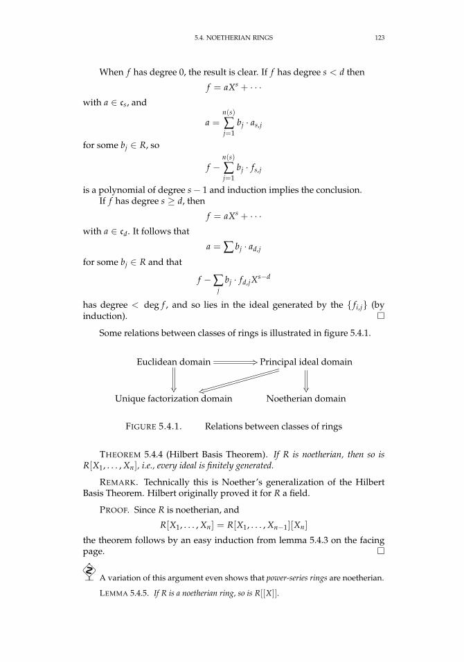
5.4. NOETHERIAN RINGS 123
When f has degree 0, the result is clear. If f has degree s < d then
f = aXs + · · ·with a ∈ cs, and
a =n(s)
∑j=1
bj · as,j
for some bj ∈ R, so
f −n(s)
∑j=1
bj · fs,j
is a polynomial of degree s− 1 and induction implies the conclusion.If f has degree s ≥ d, then
f = aXs + · · ·with a ∈ cd. It follows that
a = ∑ bj · ad,j
for some bj ∈ R and that
f −∑j
bj · fd,jXs−d
has degree < deg f , and so lies in the ideal generated by the fi,j (byinduction).
Some relations between classes of rings is illustrated in figure 5.4.1.
Euclidean domain +3
Principal ideal domain
owUnique factorization domain Noetherian domain
FIGURE 5.4.1. Relations between classes of rings
THEOREM 5.4.4 (Hilbert Basis Theorem). If R is noetherian, then so isR[X1, . . . , Xn], i.e., every ideal is finitely generated.
REMARK. Technically this is Noether’s generalization of the HilbertBasis Theorem. Hilbert originally proved it for R a field.
PROOF. Since R is noetherian, and
R[X1, . . . , Xn] = R[X1, . . . , Xn−1][Xn]
the theorem follows by an easy induction from lemma 5.4.3 on the facingpage.
A variation of this argument even shows that power-series rings are noetherian.
LEMMA 5.4.5. If R is a noetherian ring, so is R[[X]].
124 5. THE THEORY OF RINGS
REMARK. As above, a simple induction shows that
R[[X1, . . . , Xk]]
is noetherian for any finite k.
PROOF. Given a power series s ∈ R[[X]], let `(s) denote its lowest nonzerocoefficient.
Let a ⊂ R[[X]] be an ideal whose elements are
v =∞
∑i=0
c(v)iXi
with c(V)i ∈ R. Define hn ⊂ R to be composed of the nth coefficients of elements ofa whose lower coefficients vanish, i.e.
hn = c(v)n|v ∈ a, c(v)0 = · · · = c(v)n−1 = 0We claim that the hn are all ideals of R (from the way elements of R[[X]] are multi-plied). Now set
Hn =n⋃
i=0hn
Then we get an ascending chain of ideals in R
H0 ⊂ · · ·which must eventually become constant with some finitely generated ideal (sinceR is noetherian)
Hm+1 = Hm = (r0, . . . , rt)
So the ri generate all of the coefficients of all elements of a. Each of the ri is thelowest nonzero coefficient of some power series fi ∈ a. We claim that
a = ( f0, . . . , ft)
Given z = ∑∞i=0 ciXi ∈ a, we must show that there exist power-series
di = ∑∞j=0 di,jX j such that
(5.4.1) z = d1 f1 + · · ·+ dt ft
If s is the highest degree of the lowest nonzero term that occurs in the fi, we cansubtract R-linear combinations of the fi from z that will kill off all of its terms ofdegree ≤ s — giving z1. This gives the constant terms of the di, i.e. di,0.
To cancel the lowest term of z1, we know that its coefficient, cs+1, is also a linearcombination of the ri. We must multiply suitable fi by X to reach it, thus definingthe d1,i. Subtracting this linear combination gives z2.
Continuing this indefinitely results in equation 5.4.1. Despite the seeming “in-finite complexity” of z, we express it as a finite linear combination because we haveinfinite series available to us as coefficients.
We conclude this section with a result due to Emmy Noether:
LEMMA 5.4.6. Let I ⊂ R be an ideal in a noetherian ring. Then:(1) in the set of prime ideals p such that I ⊂ p, there is a minimal element(2) the set of minimal prime ideals containing I is finite.
PROOF. The first statement follows from:(1) every ideal is contained in a maximal ideal (see proposition 5.2.11 on
page 115),(2) maximal ideals are prime (see proposition 5.2.4 on page 112) so every
ideal is contained in at least one prime ideal,
5.5. POLYNOMIAL RINGS 125
(3) the intersection of a decreasing sequence of prime ideals is prime (seeexercise 6 on page 116).
We prove the second statement by contradiction. Let I denote the set of ideals withan infinite number of minimal primes that contain them. Every ascending chain ofideals in I
I1 ⊂ I2 ⊂ · · ·has an upper bound since the sequence stabilizes after a finite number of terms(this is the only place where we use the noetherian property of R). Zorn’s Lemma( A.2.12 on page 462) implies that I has a maximal member, M.
Clearly, M is not prime because it would be the (one and only) minimal primecontaining it. It follows that
(1) there exist a, b ∈ R such that a · b ∈M and a /∈M and b /∈M.(2) if A = (a,M) and B = (b,M), then M ⊂ A, M ⊂ B, and A ·B ⊂M
If pi is the infinite set of minimal primes that contain I, exercise 5 on page 115implies that, for each i, A ⊂ pi or B ⊂ pi. It follows that A or B (or both) iscontained in an infinite number of the pi — without loss of generality, we will sayit is A. Since M ( A, it follows that A can only have a finite number of minimalprimes containing it. This is the contradiction.
EXERCISES.
1. Show that every finite integral domain is a field.
2. Use the proposition 5.4.2 on page 122 to show that any quotient of anoetherian ring is noetherian.
3. Show that Q[X, Y] is not a Euclidean domain.
4. Find all the maximal ideals of Z[X].
5. Show that an element of R[[X1, . . . , Xn]] is a unit if and only if itsconstant term is a unit in R.
6. If R is a noetherian ring, show that the nilradical is nilpotent, i.e.that there exists a integer k > 0 such that N(R)k = 0.
7. Suppose p ⊂ R is a minimal prime ideal in a noetherian (commuta-tive) ring. Show that all of the elements of p are zero-divisors.
5.5. Polynomial rings
Polynomial rings are important in many areas of algebra and algebraicgeometry. Problems in important application-areas can often be reduced tocomputations in polynomial rings.
126 5. THE THEORY OF RINGS
5.5.1. Ideals and systems of equations. Suppose
W = C[X1, . . . , Xn]
suppose f1, . . . , fs ∈ W, and suppose we want to solve the system of alge-braic equations
f1(X1, . . . , Xn) = 0...
fs(X1, . . . , Xn) = 0(5.5.1)
If g1, . . . , gt ∈W is a set of polynomials with the property that
( f1, . . . , fs) = (g1, . . . , gt) = B
— i.e., the gj are another basis for the ideal generated by the fi, then theequations in 5.5.1 are equivalent to
g1(X1, . . . , Xn) = 0...
gt(X1, . . . , Xn) = 0
To see that, note that, since the fi are a basis for B and the gi ∈ B, wehave equations
gi =s
∑j=1
ai,j f j
where ai,j ∈ W for all i and j. It follows that f1 = · · · = fs = 0 implies thatg1 = · · · = gt = 0. Since the gj are also a basis for B, the reverse implicationis also true.
EXAMPLE 5.5.1. Suppose we want to find solutions to the system ofalgebraic equations
xy = z2
xz = 1
x2 + y2 = 3
We first make these into equations set to zero
xy− z2 = 0xz− 1 = 0
x2 + y2 − 3 = 0
and find another basis for the ideal these polynomials generate. It turns out1
that
(xy− z2, xz− 1, x2 + y2 − 3) = (z8 − 3z2 + 1, y− z3, z7 − 3z + x)
1This is not at all obvious! Later, we will look at an algorithm for coming to thisconclusion.
5.5. POLYNOMIAL RINGS 127
So our original equations are equivalent to the equations
z8 − 3z2 + 1 = 0
y− z3 = 0
z7 − 3z + x = 0
or
z8 − 3z2 + 1 = 0
y = z3
x = 3z− z7
so that it follows that our original set of equations had eight solutions: find8 roots of the polynomial in z and plug them into the equations for x and y.
It follows that there are applications to finding “simplified” or “im-proved” bases for ideals in polynomial rings.
5.5.2. Gröbner bases. One of the most powerful technique for compu-tations in polynomial rings use a special basis for an ideal, called a Gröbnerbasis. Gröbner bases were discovered by Bruno Buchberger (in his thesis,[20]) and named after his teacher, Wolfgang Gröbner. He refined this con-struction in subsequent papers — see [21, 22].
One key idea in the theory of Gröbner bases involves imposing an or-dering on the monomials in a polynomial ring:
DEFINITION 5.5.2. If F is a field, define an ordering on the elementsof Nn and an induced ordering on the monomials of F[X1, . . . , Xn] by α =(a1, . . . , an) β = (b1, . . . , bn) implies that
∏ Xaii ∏ Xbi
i
The ordering of Nn must satisfy the conditions:(1) if α β and γ ∈Nn, then α + γ β + γ(2) is a well-ordering: every set of elements of Nn has a minimal
element.For any polynomial f ∈ F[X1, . . . , Xn], let LT( f ) denote its leading term inthis ordering — the polynomial’s highest-ordered monomial with its coef-ficient.
REMARK. Condition 1 implies that the corresponding ordering ofmonomials is preserved by multiplication by a monomial. Condition 2implies that there are no infinite descending sequences of monomials.
DEFINITION 5.5.3. Suppose F is a field and an ordering has been cho-sen for the monomials of F[X1, . . . , Xn]. If a ∈ F[X1, . . . , Xn] is an ideal, letLT(a) denote the ideal generated by the leading terms of the polynomialsin a.
(1) If a = ( f1, . . . , ft), then f1, . . . , ft is a Gröbner basis for a if
LT(a) = (LT( f1), . . . , LT( ft))
128 5. THE THEORY OF RINGS
(2) A Gröbner basis f1, . . . , ft is minimal if the leading coefficient ofeach fi is 1 and for each i
LT( fi) /∈ (LT( f1), . . . , LT( fi−1), LT( fi+1), . . . LT( ft))
(3) A Gröbner basis f1, . . . , ft is reduced if the leading coefficient ofeach fi is 1 and for each i and no monomial of fi is contained in
(LT( f1), . . . , LT( fi−1), LT( fi+1), . . . LT( ft))
REMARK. There are many different types of orderings that can be usedand a Gröbner basis with respect to one ordering will generally not be onewith respect to another.
DEFINITION 5.5.4. The two most common orderings used are:(1) Lexicographic ordering. Let α = (a1, . . . , an), β = (b1, . . . , bn) ∈ Nn.
Then α > β ∈ Nn if, in the vector difference α − β ∈ Zn, theleftmost nonzero entry is positive — and we define
∏ Xaii ∏ Xbi
i
soXY2 Y3Z4
(2) Graded reverse lexicographic order. Here, monomials are first or-dered by total degree — i.e., the sum of the exponents. Ties areresolved lexicographically (in reverse — higher lexicographic or-der represents a lower monomial).
REMARK. In Graded Reverse Lexicographic order, we get
X4Y4Z7 X5Y5Z4
since the total degree is greater. As remarked above, Gröbner bases de-pend on the ordering, : different orderings give different bases and evendifferent numbers of basis elements.
Gröbner bases give an algorithmic procedure (detailed later) for decid-ing whether a polynomial is contained in an ideal and whether two idealsare equal.
To describe Buchberger’s algorithm for finding a Gröbner (or standard)basis, we need something called the division algorithm. This is a generaliza-tion of the usual division algorithm for polynomials of a single variable:
ALGORITHM 5.5.5 (Division Algorithm). Let be an ordering on themonomials of F[X1, . . . , Xn], where F is some field, and let A = f1, . . . , fkbe a set of polynomials. If f ∈ F[X1, . . . , Xn] is some polynomial, the divisionalgorithm computes polynomials a1, . . . , as such that
(5.5.2) f = a1 f1 + · · ·+ ak fk + R
where R = 0 or no monomial in R is divisible by LT( fi) for any i.In general, we will be more interested in the remainder, R, than the “quo-
tients” ai. We will use the notation
f →A R
to express the fact that the remainder has a certain value (“ f reduces to R”). Thealgorithm is:
5.5. POLYNOMIAL RINGS 129
function DIVISION( f , f1, . . . , fk)ai ← 0R← 0g← fwhile g 6= 0 do
Matched← Falsefor i = 1, . . . , k do
if LT( fi)∣∣LT(g) then
h← LT(g)LT( fi)
ai ← ai + hg← g− fi · hMatched← True. LT(g) was divisible by one of the LT( fi)Break . Leave the for-loop and continue the While-loop
end ifend forif not Matched then. LT(g) was not divisible by any of the LT( fi)
R← R + LT(g) . so put it into the remainderg← g− LT(g) . Subtract it from f
end ifend whilereturn f = a1 f1 + · · ·+ ak fk + R. where the monomials of R are not divisible by the leading terms of
any of the fiend function
REMARK. As is usual in describing algorithms, a ← b represents as-signment, i.e. “take the value in b and plug it into a” (the symbol ‘=’ merelystates that two quantities are equal). The symbol B denotes a comment —on how the computation is proceeding.
It should be noted that:
PROPOSITION 5.5.6. The division algorithm terminates in a finite number ofsteps and, in equation 5.5.2 on the preceding page,
(5.5.3) LT( f ) LT(ai fi)
for i = 1, . . . , k.
PROOF. The algorithm requires a finite number of steps because is awell-ordering: any decreasing sequence of monomials must terminate in a fi-nite number of steps (see the remark following definition 5.5.2 on page 127).In each iteration of the While-loop g (initially equal to f ) loses a monomialand may gain others — which are ordered lower than the one it lost.
If there existed a term ai fi with LT(ai fi) LT( f ), there would have tobe cancellation among leading terms of the ai fi, since their sum is f . Themethod used to construct the ai guarantees that
LT(ai fi) 6= LT(aj f j)
for i 6= j, so no cancellation can occur among the leading terms in equa-tion 5.5.2 on the preceding page.
130 5. THE THEORY OF RINGS
EXAMPLE 5.5.7. Let f = X2Y + XY2 + Y2, and let f1 = XY − 1 andf2 = Y2 − 1.
Assume lexicographic ordering with X Y. Then LT( f1)∣∣LT( f ) and
we get
h ← Xa1 ← Xg ← g− X · (XY− 1)
= XY2 + Y2 + X
In the second iteration of the While-loop, LT( f1)∣∣LT(g) and
h ← Ya1 ← a1 + Y
= X + Yg ← g−Y · (XY− 1)
= Y2 + X + Y
In the third iteration of the While-loop, we have LT( f1) - LT(g) and LT( f2) -LT(g) so
R ← Xg ← g− X
= Y2 + Y
In the fourth iteration of the While-loop, we have LT( f1) - LT(g) butLT( f2)
∣∣LT(g) so
h ← 1a2 ← 1g ← g− 1 · (Y2 − 1)
= Y + 1
Since neither Y nor 1 are divisible by the leading terms of the fi they arethrown into the remainder and we get
f = (X + Y) · f1 + 1 · f2 + X + Y + 1
Note that our remainder depends on the order of the polynomials. Ifwe set f1 = Y2 − 1 and f2 = XY− 1 we get
f = (X + 1) · f1 + X · f2 + 2X + 1
It turns out that the remainder can vanish with one ordering and not an-other!
With the Division Algorithm in hand, we can discuss some of the moreimportant properties of Gröbner bases:
PROPOSITION 5.5.8 (Division Property). Let be an ordering of monomi-als in F[X1, . . . , Xn] where F is a field, and let a = (g1, . . . , gk) ⊂ F[X1, . . . , Xn]be an ideal with G = g1, . . . , gk a Gröbner basis. If f ∈ F[X1, . . . , Xn], thenf ∈ a if and only if
f →G 0
5.5. POLYNOMIAL RINGS 131
PROOF. If f →G 0, then f ∈ a. Conversely, suppose f ∈ a and f →G R.If R 6= 0 then
R = f −t
∑i=1
aigi
so that R ∈ a and LT(R) ∈ LT(a) (since G is a Gröbner basis). This contra-dicts the fact that the leading term of R is not divisible by the leading termsof the gi.
This immediately implies that
COROLLARY 5.5.9. If F is a field, a ⊂ F[X1, . . . , Xn] is an ideal, and B is aminimal Gröbner basis then a = (1) if and only if B = 1.
PROOF. If 1 ∈ a, then1→B 0
which can only happen if 1 ∈ B. Since B is minimal, B = 1.
5.5.3. Buchberger’s Algorithm. We begin by proving a property thatGröbner bases have.
DEFINITION 5.5.10. If F is a field,< is some ordering on the monomialsof F[X1, . . . , Xn], and a = ( f1, · · · , ft) is an ideal, let
(5.5.4) gi,j =LT( fi)
gcd(LT( fi), LT( f j))
and define the S-polynomial
Si,j = gj,i · fi − gi,j · f j
REMARK. Note that LT(gj,i · fi) = LT(gi,j · f j) so that they cancel out inSi,j.
Buchberger’s Theorem states that the S-polynomials give a criterionfor a basis being Gröbner. It quickly leads to an algorithm for computingGröbner bases.
THEOREM 5.5.11. Let F be a field, F = f1, . . . , ft ∈ F[X1, . . . , Xn] be aset of polynomials and let be an ordering on the monomials of F[X1, . . . , Xn].Then F is a Gröbner basis of the ideal a = ( f1, . . . , ft) if and only if
Si,j →F 0
for every S-polynomial one can form from the polynomials in F.
PROOF. If F is a Gröbner basis, then the division property (proposi-tion 5.5.8 on the facing page) implies
Si,j →F 0
since Si,j ∈ a.On the other hand, suppose all S-polynomials reduce to 0. Then there
exist expressions
(5.5.5) Si,j =t
∑`=1
a`i,j f`
132 5. THE THEORY OF RINGS
for all 1 ≤ i < j ≤ t and 1 ≤ ` ≤ t such that
LT(Si,j) LT(a`i,j fi)
LT(si,j f j) LT(a`i,j fi)(5.5.6)
Suppose that F is not a Gröbner basis — i.e.LT(a) 6= (LT( f1), . . . , LT( ft)). Then there exists an elementf ∈ a with
(5.5.7) f =t
∑i=1
bi fi
such that LT( fi) - LT( f ) for all i = 1, . . . , t. The only way this can happenis if the leading terms of two of the terms in equation 5.5.7 cancel. Supposem is the highest (in the ordering) monomial of LT(bi fi) for i = 1, . . . , t,suppose f has been chosen to make m minimal, and so that m occurs aminimal number of times.
Without loss of generality, suppose that b1LT( f1) = LT(b1 f1) andb2LT( f2) = LT(b2 f2) are equal to m, up to multiplication by an element ofk. If we divide both of these by gcd(LT( f1), LT( f2)), we get
k1b1s1,2 = b2 · s2,1
where si,j is as in equation 5.5.4 on the preceding page. Since the si,j have nocommon factors, we conclude that s2,1|b1 or b1 = c · s2,1, for some monomialc, so b1LT( f1) = c · s2,1 · LT( f1). Now form the quantity
f ′ = f − c
(S1,2 −
t
∑`=1
a`1,2 f`
)(where S1,2 is as in definition 5.5.10 on the previous page).
Our hypothesis (equation 5.5.5 on the preceding page) implies that f ′ =f . On the other hand, the term −c · s2,1 · f1 in −cS1,2 cancels out b1LT( f1)and the term +c · s1,2 · f2 combines with the term b2 f2 so that the numberof occurrences of the monomial m decreases by at least 1. Equation 5.5.6 onpage 132 implies that the terms a`1,2 f` cannot affect this outcome, so wehave a contradiction to the fact that m occurred a minimal number of timesin f . We conclude that F must have been a Gröbner basis.
This result immediately leads to an algorithm for computing a Gröbnerbasis:
ALGORITHM 5.5.12 (Buchberger’s Algorithm). Given a set of polynomialsF = f1, . . . , ft ∈ F[X1, . . . , Xn],
(1) for each pair (i, j) with 1 ≤ i < j ≤ t, compute Si,j as in defini-tion 5.5.10 on the previous page,
(2) compute Si,j →F hi,j, using the Division Algorithm ( 5.5.5 on page 128),(3) if hi,j 6= 0, set
F = F ∪ hi,jand return to step 1.
The algorithm terminates when all of the hi,j found in step 3 are 0.
5.5. POLYNOMIAL RINGS 133
REMARK. The Hilbert Basis theorem ( 5.4.4 on page 123) implies thatthis process will terminate in a finite number of steps (since we are append-ing generators of LT(a)).
To get a minimal Gröbner basis, simply throw away unnecessary ele-ments. To get a reduced basis, apply the Division Algorithm to each memberof the output of this algorithm with respect to the other members.
Unfortunately, Buchberger’s algorithm can have exponentialtime-complexity — for graded-reverse lexicographic ordering — anddoubly-exponential (een
) complexity for lexicographic ordering (see [73]).This, incidentally, is why we discussed resultants of polynomials: thecomplexity of computing Gröbner bases (especially with lexicographicordering, which leads to the Elimination Property) can easily overwhelmpowerful computers. Computing resultants is relatively simple (they boildown to computing determinants).
In practice it seems to have a reasonable running time. In special cases,we have:
(1) For a system of linear polynomials, Buchberger’s Algorithm be-come Gaussian Elimination (see 6.2.30 on page 176) for putting amatrix in upper triangular form.
(2) For polynomials over a single variable, it becomes Euclid’s algo-rithm for finding the greatest common divisor for two polynomials(see 3.1.12 on page 17).
Here is an example:
EXAMPLE 5.5.13. Let f1 = XY + Y2 and f2 = X2 in F[X, Y] and wecompute a Gröbner basis using lexicographical ordering with
X Y
We have LT( f1) = XY and LT( f2) = X2. Neither is a multiple of theother and their greatest common divisor is X. Our first S-polynomial is
S1,2 =LT( f2)
Xf1 −
LT( f1)
Xf2 = XY2
The remainder after applying the Division Algorithm is−Y3 so we set f3 =Y3. We compute
S1,3 =LT( f3)
Yf1 −
LT( f1)
Yf3 = Y4
S2,3 =LT( f3)
1f2 −
LT( f2)
1f3 = 0
Since both of these are in the ideal generated by f1, f2, f3, we are done.
Gröbner bases have an interesting history. In 1899, Gordon gave a newproof of the Hilbert Basis theorem2 (theorem 5.4.4 on page 123) that demon-strated the existence of a finite Gröbner basis (with lexicographic ordering)but gave no algorithm for computing it. See [46].
2He felt that Hilbert’s proof was too abstract and gave a constructive proof.
134 5. THE THEORY OF RINGS
In 1920, Janet (see [58]) gave an algorithm for computing “involutivebases” of linear systems of partial differential equations, that can be trans-lated into Buchberger’s algorithm in a certain case. Given a system ofdifferential equations that are linear combinations of products of partialderivatives of ψ(x1, . . . , xn) (with constant coefficients), one can substitute
ψ = e∑ αixi
and get systems of polynomials in the αi whose solution leads to solutionsof the differential equations.
In 1950, Gröbner published a paper ([50]) that explored an algorithmfor computing Gröbner bases, but could not prove that it ever terminated.One of Buchberger’s signal contributions were the introduction ofS-polynomials and theorem 5.5.11 on page 131.
Teo Mora (see [75, 76]) extended much of the theory of Gröbner bases tosome non-polynomial rings, including local rings and power series rings.
At this point, we can prove another interesting property of Gröbnerbases, when computed in a certain way:
PROPOSITION 5.5.14 (Elimination Property). Suppose F is a field andg1, . . . , gj is a Gröbner basis for the ideal a ∈ F[X1, . . . , Xn], computed us-ing lexicographic ordering with
X1 X2 · · · Xn
If 1 ≤ t ≤ n, thena∩F[Xt, . . . , Xn]
has a Gröbner basis that is
g1, . . . , gj ∩F[Xt, . . . , Xn]
REMARK. This is particularly important in using Gröbner bases tosolve systems of algebraic equations. Here, we want to eliminate variablesif possible and isolate other variables. In example 5.5.1 on page 126, wehave the ideal
B = (xy− z2, xz− 1, x2 + y2 − 3)and can find a Gröbner basis for it with lexicographic ordering with x y z of
(z8 − 3z2 + 1, y− z3, z7 − 3z + x)Here, the basis element z8 − 3z2 + 1 is an element of B ∩R[z] ⊂ R[x, y, z]and the variables x and y have been eliminated from it. It follows that z,alone, must satisfy
z8 − 3z2 + 1 = 0and we can solve for x and y in terms of z.
PROOF. Suppose f ∈ a∩F[Xt, . . . , Xn] and its expansion using the Di-vision Algorithm ( 5.5.5 on page 128) is
f = ∑ qi · gi
with LT(qi · gi) LT( f ) for all i (see equation 5.5.3). Lexicographic order-ing implies that, if X1, . . . , Xt−1 occur anywhere in qi · gi then these variables
5.5. POLYNOMIAL RINGS 135
will be in the leading term of qi · gi and LT(qi · g1) LT( f ) — a contradic-tion. It follows that, for all i such that gi contains variables X1, . . . , Xt−1,the corresponding qi = 0. Since f is a linear combination of polynomialsg1, . . . , gj ∩ k[Xt, . . . , Xn], they generate a∩ k[Xt, . . . , Xn].
SinceSi,i′ →G′ 0
whenever gi, gi′ ∈ g1, . . . , gj ∩ F[Xt, . . . , Xn], theorem 5.5.11 on page 131implies that G′ = g1, . . . , gj ∩F[Xt, . . . , Xn] is a Gröbner basis.
We already know how to test membership of a polynomial in an ideal viathe Division Algorithm and proposition 5.5.8 on page 130. This algorithmalso tells us when one ideal is contained in another since ( f1, . . . , f j) ⊆(g1, . . . , g`) if and only if fi ∈ (g1, . . . , g`) for i = 1, . . . , j.
We can use Gröbner bases to compute intersections of ideals:
PROPOSITION 5.5.15 (Intersections of ideals). Let a = ( f1, . . . , f j), b =(g1, . . . , g`) be ideals in F[X1, . . . , Xn]. If we introduce a new variable, T, andcompute the Gröbner basis of
(T f1, . . . , T f j, (1− T)g1, . . . (1− T)g`)
using lexicographic ordering and ordering T higher than the other variables, theGröbner basis elements that do not contain T will be a Gröbner basis for a∩ b.
REMARK. If f , g ∈ F[X1, . . . , Xn], this allows us to compute the leastcommon multiple, z, of f and g since
(z) = ( f ) ∩ (g)
and the greatest common divisor — even if we don’t know how to factorpolynomials! If n > 1, F[X1, . . . , Xn] is not a Euclidean domain.
PROOF. Let I ∈ F[T, X1, . . . , Xn] denote the big ideal defined above.We claim that
I∩F[X1, . . . , Xn] = a∩ b
Suppose f ∈ I∩F[X1, . . . , Xn] . Then
f = ∑ aiT fi + ∑ bj(1− T)gj
= T(∑ ai fi −∑ bjgj
)+ ∑ bjgj
so
∑ ai fi −∑ bjgj = 0
It follows that f = ∑ bjgj and that ∑ ai fi = ∑ bjgj so that f ∈ a∩ b. Theconclusion now follows from the Elimination Property.
5.5.4. Mathematical software. All of the more commonly used sys-tems of mathematical software are able to compute Gröbner bases and im-plement the Division Algorithm. Among commercial systems, Maple andMathematica have very nice user-interfaces. Free software that can do thisincludes Maxima and Macaulay 2, and CoCoa. See [34] for much moreinformation.
136 5. THE THEORY OF RINGS
To use Macaulay 2, start it (in Unix-type systems) by typing M2 (thecommand is actually capitalized). The default output format is rather aw-ful, so you should change it by typing
compactMatrixForm = falseNow define a polynomial ring over Q
R = QQ[a..f,MonomialOrder=>Lex]Note that ordering is also specified here. Now define an ideal:
i3 : I = ideal(a*b*c-d*e*f,a*c*e-b*d*f,a*d*f-b*c*e)o3 = ideal (a*b*c - d*e*f, a*c*e - b*d*f,a*d*f - b*c*e)o3 : Ideal of R
To get a Gröbner basis, type:gens gb IYou need to make the window wide enough to contain the entire out-
put expression. Subscripted variables can be defined viax_2=3The ring above could have been defined viaR = QQ[x_1..x_6,MonomialOrder=>Lex]
In Maple the procedure is somewhat different: First, load the libraryvia ’with(Groebner);’. The library PolynomialIdeals is also veryuseful. Enter an ideal by simply enclosing its generators in square brackets.The command Basis computes a Gröbner basis:Basis([a*b*c-d*e*f, a*c*e-b*d*f,a*d*f-b*c*e], plex(a, b, c, d, e, f))
The output is nicely formatted.The expression plex implies lexicographic ordering, and
you must explicitly give the order of variables. For instanceplex(a, b, c, d, e, f) means
a b c d e f
Maple also supports graded lexicographic ordering with thecommand grlex(a,b,c,d,e,f) or graded reverse lexicographic ordervia tdeg(a,b,c,d,e,f).
To reduce a polynomial using the Division Algorithm ( 5.5.5 onpage 128), the Maple command is
NormalForm(list_polys,basis,monomial_order) wherethe basis need not be Gröbner. It returns a list of remainders of thepolynomials in the list.
Maxima has a package that computes Gröbner basesusing lexicographic ordering (at present, no other orderingis available). To load it, type load(grobner). The maincommands are poly_grobner(poly-list,var-list), andpoly_reduced_grobner(poly-list,var-list). For example:
poly_grobner([x^2+y^2,x^3-y^4],[x,y]); returns
(x2 + y2, x3 − y4, x4 + xy2, y6 + y4)
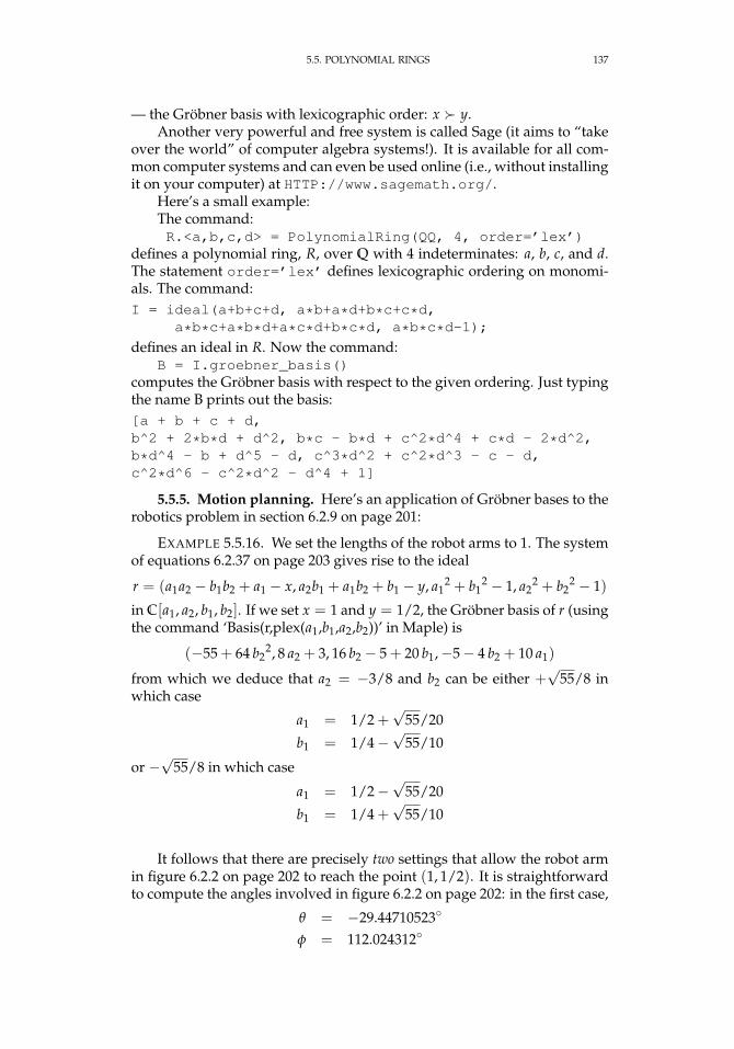
5.5. POLYNOMIAL RINGS 137
— the Gröbner basis with lexicographic order: x y.Another very powerful and free system is called Sage (it aims to “take
over the world” of computer algebra systems!). It is available for all com-mon computer systems and can even be used online (i.e., without installingit on your computer) at HTTP://www.sagemath.org/.
Here’s a small example:The command:R.<a,b,c,d> = PolynomialRing(QQ, 4, order=’lex’)
defines a polynomial ring, R, over Q with 4 indeterminates: a, b, c, and d.The statement order=’lex’ defines lexicographic ordering on monomi-als. The command:I = ideal(a+b+c+d, a*b+a*d+b*c+c*d,
a*b*c+a*b*d+a*c*d+b*c*d, a*b*c*d-1);
defines an ideal in R. Now the command:B = I.groebner_basis()
computes the Gröbner basis with respect to the given ordering. Just typingthe name B prints out the basis:[a + b + c + d,b^2 + 2*b*d + d^2, b*c - b*d + c^2*d^4 + c*d - 2*d^2,b*d^4 - b + d^5 - d, c^3*d^2 + c^2*d^3 - c - d,c^2*d^6 - c^2*d^2 - d^4 + 1]
5.5.5. Motion planning. Here’s an application of Gröbner bases to therobotics problem in section 6.2.9 on page 201:
EXAMPLE 5.5.16. We set the lengths of the robot arms to 1. The systemof equations 6.2.37 on page 203 gives rise to the ideal
r = (a1a2 − b1b2 + a1 − x, a2b1 + a1b2 + b1 − y, a12 + b1
2 − 1, a22 + b2
2 − 1)
in C[a1, a2, b1, b2]. If we set x = 1 and y = 1/2, the Gröbner basis of r (usingthe command ‘Basis(r,plex(a1,b1,a2,b2))’ in Maple) is
(−55 + 64 b22, 8 a2 + 3, 16 b2 − 5 + 20 b1,−5− 4 b2 + 10 a1)
from which we deduce that a2 = −3/8 and b2 can be either +√
55/8 inwhich case
a1 = 1/2 +√
55/20
b1 = 1/4−√
55/10
or −√
55/8 in which case
a1 = 1/2−√
55/20
b1 = 1/4 +√
55/10
It follows that there are precisely two settings that allow the robot armin figure 6.2.2 on page 202 to reach the point (1, 1/2). It is straightforwardto compute the angles involved in figure 6.2.2 on page 202: in the first case,
θ = −29.44710523
φ = 112.024312
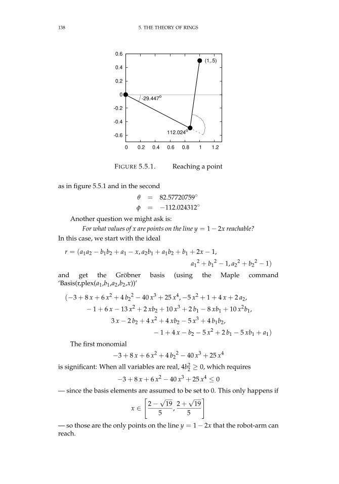
138 5. THE THEORY OF RINGS
-0.6
-0.4
-0.2
0
0.2
0.4
0.6
0 0.2 0.4 0.6 0.8 1 1.2
-29.447o
112.024o
(1,.5)
FIGURE 5.5.1. Reaching a point
as in figure 5.5.1 and in the second
θ = 82.57720759
φ = −112.024312
Another question we might ask is:For what values of x are points on the line y = 1− 2x reachable?
In this case, we start with the ideal
r = (a1a2 − b1b2 + a1 − x, a2b1 + a1b2 + b1 + 2x− 1,
a12 + b1
2 − 1, a22 + b2
2 − 1)
and get the Gröbner basis (using the Maple command‘Basis(r,plex(a1,b1,a2,b2,x))’
(−3 + 8 x + 6 x2 + 4 b22 − 40 x3 + 25 x4,−5 x2 + 1 + 4 x + 2 a2,
− 1 + 6 x− 13 x2 + 2 xb2 + 10 x3 + 2 b1 − 8 xb1 + 10 x2b1,
3 x− 2 b2 + 4 x2 + 4 xb2 − 5 x3 + 4 b1b2,
− 1 + 4 x− b2 − 5 x2 + 2 b1 − 5 xb1 + a1)
The first monomial
−3 + 8 x + 6 x2 + 4 b22 − 40 x3 + 25 x4
is significant: When all variables are real, 4b22 ≥ 0, which requires
−3 + 8 x + 6 x2 − 40 x3 + 25 x4 ≤ 0
— since the basis elements are assumed to be set to 0. This only happens if
x ∈[
2−√
195
,2 +√
195
]— so those are the only points on the line y = 1− 2x that the robot-arm canreach.
5.5. POLYNOMIAL RINGS 139
We can also analyze the Puma-type robot-arm in figure 6.2.3 onpage 203:
EXAMPLE 5.5.17. If we set `1 = `2 = 1, equation 6.2.38 on page 205implies that the endpoint of the robot-arm are solutions to the system
a5a4a3 − a5b4b3 + a5a4 − x = 0b5a4a3 − b5b4b3 + b5a4 − y = 0
b4a3 + a4b3 + b4 − z = 0a2
3 + b23 − 1 = 0
a24 + b2
4 − 1 = 0
a25 + b2
5 − 1 = 0(5.5.8)
If we want to know which points it can reach with the hand pointing in thedirection 1/
√3
1/√
31/√
3
use equation 6.2.39 on page 205 to get
(a5a4a3 − a5b4b3) a2 + (−a5a4b3 − a5b4a3) b2 − 1/√
3 = 0
(b5a4a3 − b5b4b3) a2 + (−b5a4b3 − b5b4a3) b2 − 1/√
3 = 0
(b4a3 + a4b3) a2 + (a4a3 − b4b3) b2 − 1/√
3 = 0
a22 + b2
2 − 1 = 0(5.5.9)
We regard these terms (in equations 5.5.8 and 5.5.9 as generators ofan ideal, P. The variety V (P) ⊂ R10 is called the variety of the movementproblem. Its (real-valued) points correspond to possible configurations ofthe robot-arm.
To understand V (P), we compute a Gröbner basis of P with lexico-graphic ordering — giving the lowest weight to x, y, z — to get
(5.5.10) P = (4 y2x2 − 4 z2 + z4 + 2 z2x2 + 2 y2z2,
− 1 + 2 b52,−b5 + a5, 2 zb4 − z2 − 2 yx,
− 4 z + 4 yb4x + z3 − 2 xzy + 2 y2z + 2 x2z,
− 2− 2 yx + 2 b42 + y2 + x2,
a4 − b5y + b5x,
− b5yz + b5xz + b3 + 2 b5yb4,
2 + 2 a3 − 2 y2 − z2,
2 b5z√
3−√
3b5y−√
3b5x− 2 b4√
3b5 + 3 b2,
3 a2 − y√
3− x√
3− z√
3 + b4√
3)
It follows that a point (x, y, z) is reachable (with the hand oriented as stated)only if it lies on the surface
4 y2x2 − 4 z2 + z4 + 2 z2x2 + 2 y2z2 = 0
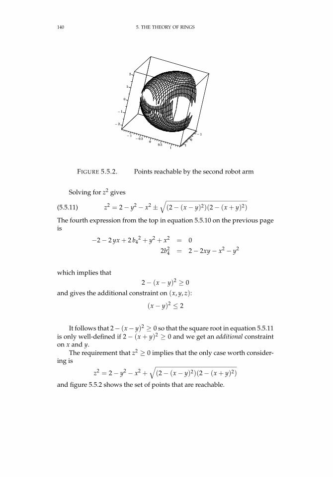
140 5. THE THEORY OF RINGS
− 1− 1
00
− 2− 2
− 1− 1− 0.5− 0.5
11
− 1− 1
000.50.5
00
11
11
22
FIGURE 5.5.2. Points reachable by the second robot arm
Solving for z2 gives
(5.5.11) z2 = 2− y2 − x2 ±√(2− (x− y)2)(2− (x + y)2)
The fourth expression from the top in equation 5.5.10 on the previous pageis
−2− 2 yx + 2 b42 + y2 + x2 = 0
2b24 = 2− 2xy− x2 − y2
which implies that2− (x− y)2 ≥ 0
and gives the additional constraint on (x, y, z):
(x− y)2 ≤ 2
It follows that 2− (x− y)2 ≥ 0 so that the square root in equation 5.5.11is only well-defined if 2− (x + y)2 ≥ 0 and we get an additional constrainton x and y.
The requirement that z2 ≥ 0 implies that the only case worth consider-ing is
z2 = 2− y2 − x2 +√(2− (x− y)2)(2− (x + y)2)
and figure 5.5.2 shows the set of points that are reachable.
5.5. POLYNOMIAL RINGS 141
EXERCISES.
1. The point (1/2, 1/2, 1 +√
2/2) lies on the “reachability surface” inexample 5.5.17 on page 139 that can be reached by the robot arm with itshand pointed in the direction
1√3
111
Find the angles φ1, θ1, θ2, θ3 that accomplish this.
2. Find the reachability surface of the robot arm in example 5.5.17 onpage 139 when we require the “hand” to point in the direction 1
00
3. Find the least common multiple of the polynomials
−X3 − 2 YX2 − XY2 + 2 X
and
4− 4 X2 − 4 Y2 + X4 − 2 Y2X2 + Y4
in F[X, Y].
4. Consider the ideal a = (Y3, X−Y).Is X + Y ∈ a?
5. If a = (Y6,−3 Y5 + 5 XY4, X2 − 2 XY +Y2) is a Gröbner basis for anideal, what is the lowest power of X + Y that is contained in a?
6. Find the least common multiple of the polynomials
−X3 − 2 YX2 − XY2 + 2 X
and
4− 4 X2 − 4 Y2 + X4 − 2 Y2X2 + Y4
in F[X, Y].
7. Consider the ideal a = (Y3, X−Y).Is X + Y ∈ a?
8. If a = (Y6,−3 Y5 + 5 XY4, X2 − 2 XY +Y2) is a Gröbner basis for anideal, what is the lowest power of X + Y that is contained in a?
142 5. THE THEORY OF RINGS
5.5.6. Elementary symmetric functions. If R is a commutative ring,consider the polynomial ring
P = R[X1, . . . , Xn]
The symmetric group, Sn, acts on this ring by permuting the variables.Each such permutation of the variables defines an automorphism of P sothe set of elements
S = R[X1, . . . , Xn]Sn
fixed by the action of Sn is a subring of P. It is interesting that the structureof this subring is completely understood — and was in the time of IsaacNewton. The actual description of this subring will be important in thesequel and is used in several areas of algebra and algebraic geometry.
In order to give this description, we will need to define the elementarysymmetric functions. The quickest (if not the simplest) way to describethem is to consider a polynomial in the ring P[T] where T is a new indeter-minate:
n
∏i=1
(T − Xi) = q(T)(5.5.12)
= Tn − σ1 · Tn−1 + · · ·+ (−1)nσn
Since q(T) is unchanged when the Xi’s are permuted, the coefficients ofq(T) must be functions of the Xi that are also unchanged by permuting theXi. They are
σ0(X1, . . . , Xn) = 1
σ1(X1, . . . , Xn) =n
∑i=1
Xi
σ2(X1, . . . , Xn) = ∑1≤i<j≤n
XiXj
...
σn(X1, . . . , Xn) =n
∏i=1
Xi(5.5.13)
where σi(X1, . . . , Xn) is (−1)i× the coefficient of tn−i.If we consider the ring R[σ1, . . . , σn] of polynomials of the σi, it is clear
thatR[σ1, . . . , σn] ⊂ R[X1, . . . , Xn]
and even thatR[σ1, . . . , σn] ⊂ R[X1, . . . , Xn]
Sn = Ssince the σi are unchanged by permutations of the Xi. It is remarkable that:
THEOREM 5.5.18. The subring of polynomials of
R[X1, . . . , Xn]
that are invariant under all permutations of the Xi is precisely the polynomial ringof elementary symmetric functions, i.e.
5.5. POLYNOMIAL RINGS 143
R[σ1, . . . , σn] = R[X1, . . . , Xn]Sn
PROOF. Let p(X1, . . . , Xn) ∈ R[X1, . . . , Xn]Sn . We will express this as apolynomial of the elementary symmetric functions. Suppose
m = r · Xα11 · · ·Xαn
n
is a monomial of p, where r ∈ R. Since p is invariant under permutations ofthe Xi, p also contains an ordered-monomial that is equivalent to m underthe action of Sn, where an ordered monomial is of the form
r · Xβ11 · · ·X
βnn
where β1 ≥ β2 ≥ · · · ≥ βn where the βi’s are some permutation of theαi’s. We may focus our attention entirely on ordered-monomials of thistype, since every monomial will be equivalent to one of these. The (unique)ordered monomial of σi(X1, . . . , Xn) is
(5.5.14) X1 · · ·Xi
Now we order the ordered-monomials of p(X1, . . . , Xn) lexicographi-cally by exponents, i.e. so
Xα11 · · ·Xαn
n Xβ1 · · ·Xβnn
if αj > β j and αi = βi, for i = 1 . . . j− 1.The polynomial p will contain a unique maximal ordered-monomial,
say
r · Xβ11 · · ·X
βnn
and this agrees with the unique maximal ordered monomial of
(5.5.15) r · σβnn · σβn−1−βn
n−1 · · · σβ1−β21
by equation 5.5.14. It follows that the unique maximal ordered monomialof
p− r · σβnn · σβn−1−βn
n−1 · · · σβ1−β21
is strictly ≺ r · Xβ11 · · ·X
βnn . Since there are only a finite number of mono-
mials ≺ r · Xβ11 · · ·X
βnn , repeating this procedure over and over again must
terminate after a finite number of steps. The polynomial p is equal to thesum of the symmetric polynomials we subtracted from p.
The proof gives us an algorithm for computing the expression of sym-metric polynomials in terms of symmetric functions:
EXAMPLE. Consider
X2 + Y2 ∈ Q[X, Y]
The maximal ordered monomial of this is X2 — which corresponds to σ21 in
equation 5.5.15. The difference is
X2 + Y2 − σ21 = X2 + Y2 − (X + Y)2
= −2XY
144 5. THE THEORY OF RINGS
which is equal to −2σ2. So we get
X2 + Y2 = σ21 − 2σ2
An interesting consequence of formula 5.5.12 on page 142 and theo-rem 5.5.18 on page 142 is:
PROPOSITION 5.5.19. Let Xn + an−1Xn−1 + · · · + a0 = p(X) ∈ Q[X]and suppose q(X1, . . . , Xn) ∈ Q[X1, . . . , Xn] is invariant under permutations ofthe Xi. If µ1, . . . , un ∈ C are the roots of p(X), then there exists a polynomialz(X1, . . . , Xn) such that
q(µ1, . . . , µn) = z(a0, . . . , an−1)
PROOF. Theorem 5.5.18 on page 142 implies thatq(X1, . . . , Xn) = z(σ1, . . . , σn). Equation 5.5.12 on page 142 shows thatσi(µ1, . . . , µn) = (−1)ian−i and the result follows.
This has an interesting application in the definition of discriminants ofpolynomials:
DEFINITION 5.5.20. Let p(x) ∈ Q[x] be of degree n with rootsα1, . . . , αn ∈ C. The discriminant, D, of p(X) is defined to be
D = ∏1≤i<j≤n
(αi − αj)2
REMARK. The discriminant is nonzero if and only if p(X) has n distinctroots (so it discriminates between roots).
Since the discriminant is unchanged by a permutation of the roots,proposition 5.5.19 implies that
COROLLARY 5.5.21. If
p(X) = Xn + an−1Xn−1 + · · ·+ a0
there is a polynomial function z(a0, . . . an−1) equal to the discriminant of p(X).
For instance, the discriminant of X2 + aX + b is
(α1 − α2)2 = α2
1 − 2α1α2 + α22
= σ21 (α1, α2)− 4α1α2
= σ21 (α1, α2)− 4σ2(α1, α2)
= a2 − 4b
A lengthy calculation shows that the discriminant of X3 + aX2 + bX + cis
D = a2b2 − 4b3 − 4a3c− 27c2 + 18abc
5.6. UNIQUE FACTORIZATION DOMAINS 145
EXERCISES.
9. Express X3 + Y3 + Z3 ∈ Q[X, Y, Z] in terms of elementary symmet-ric functions.
10. Show that the discriminant of Xn − 1 is ±nn.
11. Let p1, p2 ∈ Q[t] are monic polynomials with roots α1, . . . , αn ∈ C
and β1, . . . , βm ∈ C, respectively. Let
∆ = ∏(αi − β j)
with i running from 1 to n and j running from 1 to m. Show that ∆ is apolynomial function of the coefficients of p1 and p2.
12. Another way of defining the discriminant involves using the Van-dermonde matrix. Given elements α1, . . . , αn, we define the correspondingVandermonde matrix as
V =
1 α1 α2
1 · · · αn−11
1 α2 α22 · · · αn−1
21 α3 α2
3 · · · αn−13
......
.... . .
...1 αn α2
n · · · αn−1n
Show that
det V = ∏1≤i<j≤n
(αj − αi)
13. Suppose F is a field and
I ⊂ F[X1, . . . , Xn]
is an ideal. If f (X1, . . . , Xn) ∈ F[X1, . . . , Xn] is any polynomial, show that
F[X1, . . . , Xn]
I∼= F[X1, . . . , Xn+1]
I+ (Xn+1 − f (X1, . . . , Xn))
In other words, show that a variable, like Xn+1, that can be expressed interms of the others is superfluous.
5.6. Unique factorization domains
5.6.1. Introduction. This section is one of the most complex inthe chapter on commutative algebra and most of it is flagged with adangerous bend symbol. We study the important question of when aring has unique factorization. Aside from any inherent interest, uniquefactorization has geometric implications that will become apparent later.
A great deal of this material is due to Gauss in his groundbreaking [41],and Weierstrass (in [107]) in his research on complex analysis in severalvariables.
146 5. THE THEORY OF RINGS
Johann Carl Friedrich Gauss (1777 – 1855) was a German mathematicianand scientist who contributed to many fields, including number theory,analysis, statistics (the normal distribution curve), differential geometry (heessentially invented it), geophysics, electrostatics, astronomy, and optics.
We can characterize unique factorization domains by
LEMMA 5.6.1. If R is a ring, the following three statements are equivalent(1) R is a unique factorization domain(2) For any r, p, q ∈ R such that
r∣∣ p · q
with r irreducibler - p =⇒ r
∣∣ q(3) For any r, p, q ∈ R such that
r∣∣ p · q
and r and p have no common factors
r - p =⇒ r∣∣ q
(4) For any irreducible element r ∈ R, the principal ideal (r) ⊂ R is prime.
REMARK. Prime ideals play an important part in algebraic geometry,and statement 4 implies that they can have a particularly simple structure.
PROOF. If statement 1 is true, then R is a unique factorization domainby reasoning like that used in lemma 3.1.9 on page 3.1.9. Conversely, if R isa unique factorization domain, then
p = u1
m
∏i=1
pβii
q = u2
m
∏i=1
pγii(5.6.1)
where u1, u2 ∈ R are units, the pi ∈ R are irreducible elements and theαi, βi, γi ∈ Z are all ≥ 0. If r|p · q, then r must equal one of the pi, say pjand αj + β j ≥ 1. Since r - p, we get αj = 0, which implies that β j ≥ 1 andthis proves the conclusion.
Statement 3 implies statement 2. Conversely, if statement 2 is true, R isa unique factorization domain and equation 5.6.1 holds as well as
r = u0
m
∏i=1
pαii
Since r has no common factors with p, αi > 0 implies that βi = 0, henceαi ≤ γi for all i = 1, . . . , n. This implies that r|q.
To see statement 4, suppose a, b ∈ U and a · b ∈ (r) or ra · b. Theprevious statement implies that r|a or r|b which means a ∈ (r) or b ∈ (r).The implication clearly goes in the opposite direction too.
One of the easiest results in this section is:
5.6. UNIQUE FACTORIZATION DOMAINS 147
LEMMA 5.6.2. If F is a field, then F[X] is a unique factorization domain.
PROOF. It is a Euclidean domain in the sense of definition 5.3.3 onpage 118 so it is also a unique factorization domain by corollary 5.3.7 onpage 118.
Even though the ideals in a unique factorization might not all be prin-cipal, we have:
PROPOSITION 5.6.3. In a unique factorization domain, the concept of great-est common divisor and least common multiple are well-defined.
REMARK. In general, we have no analogue of the Euclidean Algorithm,so it may be impossible to have a formula like equation 3.1.1 on page 14.
PROOF. If U is a unique factorization domain with elements x and y,then they have factorizations, unique up to multiplication by units. Letp1, . . . , pk be all of the irreducible factors that occur in their factorizations:
x = uk
∏i=1
pαii
y = u′k
∏i=1
pβii
Now we can define
gcd(x, y) =k
∏i=1
pmin(αi ,βi)i
lcm(x, y) =k
∏i=1
pmax(αi ,βi)i
5.6.2. Polynomial rings. Throughout the rest of this section, we fix aunique factorization domain, U. We will show that U[X] is also a uniquefactorization domain. We use a trick to prove this: embed U[X] in F[X],where F is the field of fractions of U and uniquely factor elements there.
The proof involves several steps.
DEFINITION 5.6.4. A polynomial anXn + · · ·+ a0 ∈ U[X] will be calledprimitive, if the greatest common divisor of its coefficients is 1.
Note that if f ∈ U[X] is a polynomial, we can write f = u · f ′ where uis the greatest common divisor of the coefficients of f and f ′ is primitive.
The following result is called Gauss’s Lemma:
LEMMA 5.6.5. If f , g ∈ U[X] are primitive polynomials, then so is f g.
REMARK. This and the following lemma were proved by Carl FriedrichGauss in his treatise [41].
148 5. THE THEORY OF RINGS
PROOF. Suppose
f = anXn + · · ·+ a0
g = bmXm + · · ·+ b0
f g = cn+mXn+m + · · ·+ c0
If d ∈ U is irreducible, it suffices to prove that d does not divide all of theci. Let ai and bj be the first coefficients (i.e. with the lowest subscripts) notdivisible by d. We claim that ci+j is not divisible by d. Note that
ci+j = a0bi+j + · · ·+ ai−1bj+1︸ ︷︷ ︸Group 1
+aibj + ai+1bj−1 + · · ·+ ai+jb0︸ ︷︷ ︸Group 2
By construction, d divides all of the terms in Group 1 and Group 2. SinceU is a unique factorization domain, d|ci+1 if and only if d|aibj. But, the factthat U is a unique factorization domain also implies that d|aibj if and onlyif d|ai or d|bj.
This leads to the following:
LEMMA 5.6.6. Let f ∈ U[X] be primitive. Then f is irreducible in U[X] ifand only if it is irreducible in F[X], where F is the field of fractions of U.
PROOF. Suppose f is irreducible in U[X], and that f = gh ∈ F[X]. Byclearing denominators, we can assume
g = u−11 g
h = u−12 h
where g, h are primitive polynomials of U[X], and u1, u2 ∈ U. We concludethat
u1u2 f = gh
where gh is primitive by 5.6.5 on the previous page. Since f is also primi-tive, the factor u1u2 ∈ U must be a unit. Since f is irreducible in U[X], g orh must be a unit in U[X] and also in F[X].
On the other hand, suppose f ∈ U[X] is irreducible in F[X] and assumef = gh ∈ U[X]. Since f is irreducible in F[X], either g or h must be a unitin F[X], i.e. a constant polynomial. If g is a constant polynomial then theformula f = gh with f primitive implies that g ∈ R is a unit.
We are finally ready to prove:
THEOREM 5.6.7. If U be a unique factorization domain, then so is U[X].
REMARK. This is interesting because U doesn’t have to be a euclideandomain or a principal ideal domain.
PROOF. We use a trick to prove this: embed U[X] in F[X], where Fis the field of fractions of U and uniquely factor elements there. Supposer, f , g ∈ U[X] are polynomials and
(1) r is irreducible.(2) r
∣∣ f g
5.6. UNIQUE FACTORIZATION DOMAINS 149
We will show that r∣∣ f or r
∣∣ g and lemma 5.6.1 on page 146 will show thatU[x] has unique factorization.
Lemma 5.6.2 on page 147 implies that F[X] is a unique factorizationdomain because it is Euclidean.
Write
r = ur′
f = u1 f ′
g = u2g′
where u, u1, u2 ∈ U are, respectively, the greatest common divisors of thecoefficients of r, f , g and r′, f ′, g′ ∈ U[x] are primitive. Since r is irreducible,we can assume u ∈ U is a unit (otherwise r = ur′ would be a nontrivialfactorization of r).
Lemma 5.6.6 on the facing page implies that r′ is irreducible in F[X] so,in F[X], r′| f ′ or r′|g′ in F[x]. Without loss of generality, assume r′| f ′, so that
f ′ = a · r′
where a ∈ F[X]. We can write a = v−1a′, where v ∈ U and a′ ∈ U[X] isprimitive. We get
v · f ′ = a′ · r′in U[X]. Since f ′ and a′ · r′ are both primitive (by lemma 5.6.5 on page 147),v ∈ U must be a unit and we get r| f .
REMARK. Actually finding factorizations in these rings can be challeng-ing.
To actually find a factorization of a polynomial, it is helpful to have acriterion for irreducibility. The following is called Eisenstein’s Criterion:
THEOREM 5.6.8. Let U be a unique factorization domain and let
f (X) = anXn + · · ·+ a0 ∈ U[X]
be a primitive polynomial and let p ∈ U be irreducible. If p∣∣ ai for 0 ≤ i ≤ n− 1,
p - an, and p2 - a0 then f (X) is irreducible in U[X].
REMARK. If F is the field of fractions of U, lemma 5.6.6 on the facingpage shows that this criterion works for polynomials over F[X] too, afterclearing the denominators of the coefficients.
Eisenstein originally proved this for Z[X] but it works for any uniquefactorization domain.
PROOF. We will reason by contradiction. Suppose there exist polyno-mials
p(X) = bsXs + · · ·+ b0
q(X) = ctXt + · · ·+ c0
such that f (X) = p(X) · q(X) and s ≥ 1 and t ≥ 1. Since p2 - a0 we musthave p - b0 or p - c0. Assume that p|c0 and p - b0. Since f is primitive, notall the ci are divisible by p. Suppose ck is the first that is not divisible by p.Then
ak = bkc0 + · · ·+ b0ck
150 5. THE THEORY OF RINGS
By assumption, p|ak and p|ci for 0 ≤ i < k, which implies that p|b0ckand this implies that p|b0, which is a contradiction.
EXAMPLE. The polynomial X3 + 3X2 + 3X + 1 ∈ Q[X] is irreducibleby Eisenstein’s Criterion with respect to the prime p = 3.
EXAMPLE 5.6.9. In some cases, one must first transform the polynomiala bit to use Eisenstein’s Criterion. For instance, in the polynomial
f (X) = X2 + X + 1 ∈ Q[X]
there are no primes that divide any of the coefficients. After substitutingX = U + 1, f (X) becomes
g(U) = U2 + 3U + 3
which satisfies Eisenstein’s Criterion with respect to the prime p = 3. SinceX → U + 1 defines an isomorphism
Q[X]→ Q[U]
f (X) is irreducible if and only if g(U) is.
5.6.3. Power-series rings. Next, we tackle the question of unique fac-torization in power series rings. This appears daunting at first glance be-cause power series seem to have “infinite complexity”. For instance, it isnot true that whenever U is a unique factorization domain, U[[X]] is also —see [96].
It is gratifying to see that, in some cases, factorization is actually easierin power series rings. The point is that factorizations are only well-definedup to multiplication by a unit — and the power series ring F[[X]] (for F afield) has many units: Proposition 5.1.9 on page 109 shows that any powerseries
z =∞
∑n=0
cnXn
with c0 6= 0 is a unit. If the lowest nonzero coefficient in z is cr then ourunique factorization of z is
(5.6.2) Xr · (cr + cr+1X + · · · )In other words, X is our “only prime” in F[[X]], and an arbitrary elementof F[[X]] is the product of a polynomial in X and a unit.
This will turn out to be true in general: the Weierstrass Preparation The-orem will show that certain elements (every element can be transformedinto one of these — see lemma 5.6.15 on page 153) of
F[[X1, . . . , Xn]]
will equal units × polynomials in
F[[X1, . . . , Xn−1]][Xn]
i. e., polynomials in Xn with coefficients in F[[X1, . . . , Xn−1]]. Unique fac-torization in F[[X1, . . . , Xn−1]] and F[[X1, . . . , Xn−1]][Xn] will imply it inF[[X1, . . . , Xn]] (via lemma 5.6.1 on page 146).
We will fix the following notation throughout the rest of thissection: Pn = F[[X1, . . . , Xn]], where F is a field.
5.6. UNIQUE FACTORIZATION DOMAINS 151
We need to develop some properties of power-series rings.
PROPOSITION 5.6.10. An element p ∈ Pn is a unit if and only if its constant term isnonzero.
PROOF. Straightforward induction using proposition 5.1.9 on page 109 and ex-ercise 3 on page 115.
DEFINITION 5.6.11. An element p(X1, . . . , Xn) ∈ Pn will be called Xn-generalif p(0, . . . , 0, Xn) 6= 0. If Xd
n∣∣ p(0, . . . , 0, Xn) and Xd+1
n - p(0, . . . , 0, Xn) for someinteger d > 0, we say that p is Xn-general of degree d.
REMARK. A power series is Xn-general if it has a term that only involves Xn.For instance X1 + X2 is X2-general but X1X2 is not.
Next, we have a kind of division algorithm for power-series rings (even thoughthese rings are not Euclidean):
THEOREM 5.6.12 (Weierstrass Division Theorem). Let p ∈ Pn be Xn-generalpower-series of degree d that is not a unit of Pn. For every power series g ∈ Pn, thereexists a power series u ∈ Pn and a polynomial r ∈ Pn−1[Xn] of degree d− 1 such that
(5.6.3) g = u · p + r
The power-series u and polynomial r are uniquely determined.
REMARK. A shorter way to say this is that
Pn
(p)= Pn−1 ⊕ Xn · Pn−1 ⊕ · · · ⊕ Xd−1
n Pn−1
or that it is a module over Pn−1 generated by 1, . . . , Xd−1n .
PROOF. We will explicitly construct u and r.For every f ∈ Pn, let r( f ) equal the set of terms, T, such that Xd
n - T, and leth( f ) be the factor of Xd
n in f − r( f ). Then
f = r( f ) + Xdnh( f )
for all power series in Pn. So r( f ), h( f ) ∈ Pn and r( f ) is a polynomial in Pn−1[Xn]of degree < d. Note that, regarding Pn as a vector space (see definition 6.2.1 onpage 163) over k, both r(∗) and h(∗) are linear maps.
CLAIM 5.6.13. In addition, h(p) is a unit (since its constant term is the elementof k multiplying Xd
n, and r( f ) has no constant terms since f is not a unit.
We claim that equation 5.6.3 is equivalent to
(5.6.4) h(g) = h(u · p)for some u ∈ Pn. If equation 5.6.3 holds then h(g − u · p) = 0 and equation 5.6.4is true. Conversely, if equation 5.6.4 on page 151is true, then h(g− u · p) = 0 andg− u · p = r(q− u · p), a degree d− 1 polynomial in Pn−1[Xn].
Since p = r(p) + Xdn · h(p), equation 5.6.4 is equivalent to
(5.6.5) u · p = u · r(p) + Xdn · u · h(p)
Since h(p) is a unit (see the claim above), it suffices to compute the power-seriesv = u · h(p). Set
m = −r( f ) · h(p)−1
152 5. THE THEORY OF RINGS
Then u · r(p) = −m · v and we can rewrite equation 5.6.5 on the previous page tothe equivalent equation
(5.6.6) h(g) = −h(m · v) + v
or
(5.6.7) v = h(g) + s(v)
where, for any power series, f ∈ Pn, we have defined s( f ) = h(m · f ). Note that sis a linear operation on power-series.
Let m = (X1, . . . , Xn−1) ⊂ Pn−1 be the maximal ideal. Note that r(p) ∈m[Xn] ⊂ Pn−1[Xn] since it is not a unit (so it has vanishing constant term). Thismeans that, if the coefficients of f ∈ Pn = Pn−1[[Xn]] lie in mj, then the coefficientsof s( f ) will lie in mj+1.
Now we plug equation 5.6.7 into itself to get
v = h(g) + s(h(g) + s(v))
= h(g) + s(h(g)) + s2(v)
We can iterate this any number of times:
v =t
∑j=0
sj(h(g)) + st+1(v)
or
v−t
∑j=0
sj(h(g)) ∈ mt+1[[Xn]] ⊂ Pn−1[[Xn]]
Since lemma 6.3.34 on page 244 implies that∞⋂
j=1mj = (0)
we claim that
v =∞
∑j=0
sj(h(g))
is the unique solution to our problem. It is easy to verify that it satisfies equa-tion 5.6.7. Now all we have to do is set
u = v · h(p)−1
and r = r(q− u · p).
The Weierstrass Preparation Theorem is a simple corollary:
THEOREM 5.6.14 (Weierstrass Preparation Theorem). Let p ∈ Pn be Xn-generalpower-series of degree d that is not a unit of Pn. Then there exists a unit u ∈ Pn and amonic polynomial w ∈ Pn−1[Xn] of degree d such that
(5.6.8) p = u · wand u and w are uniquely determined by p.
REMARK. This is the general analogue of 5.6.2 on page 150 for power-series ofn variables. Weierstrass originally proved it for convergent power series using themethods of complex analysis. It gives valuable information on the behavior of thezero-sets of analytic functions of several complex variables (besides implying thatthe ring of such functions has unique factorization).
Our proof of the Division Theorem is the “combinatorial” or “algebraic” form— that does not use contour integrals.
The polynomial w ∈ Pn−1[Xn] is called the Weierstrass Polynomial of p.

5.6. UNIQUE FACTORIZATION DOMAINS 153
Case 1. Apply the division theorem ( 5.6.12 on page 151) to g = Xdn. It gives q and
r such thatXd
n = q · p + rso we get
q · p = Xdn − r = w ∈ Pn−1[Xn]
We claim that q must be a unit since the lowest Xn term in p is Xdn. The
only way the product could contain Xdn is for u to have a nonvanishing
constant term. Now set u = q−1, so that p = u · w.If A is an n× n invertible matrix whose entries are in k, then A induces an automor-phism
A∗: Pn → Pn
p(X1, . . . , Xn) 7→ pA = p(A−1 · (X1, . . . , Xn))
The inverse is given by the inverse of A.
LEMMA 5.6.15. Let p ∈ Pn be a power series that is not a unit. If the field F isinfinite, then there exists a matrix, A, such that pA is Xn-general.
PROOF. Let L be the leading term of p — this consists of the terms of lowest to-tal degree in the power series and will be a homogeneous polynomial in X1, . . . , Xn.Let
(k1, . . . , kn) ∈ Fn
be a set of values on which L is nonvanishing. Such a set of values exists becausewe can plug in 1 for all of the Xi except one, and the resulting polynomial of onevariable vanishes at a finite number of values. Since the field F is infinite, we canfind a value for the remaining variable that makes L 6= 0 vanish. Let A be aninvertible matrix that transforms this point
(k1, . . . , kn)
to (0, . . . , 0, 1). The conclusion follows.
It is easy (and necessary) to generalize this a bit:
COROLLARY 5.6.16. Let p1, . . . , pt ∈ Pn be a finite set of power series that are non-units. Then there exists an invertible matrix A such that pA
1 , . . . , pAt ∈ Pn are all Xn-
regular.
PROOF. Simply apply lemma 5.6.15 to the product p1 · · · pt.
We are finally ready to prove the main result:
THEOREM 5.6.17. If F is an infinite field, then the ring Pn = F[[X1, . . . , Xn]] is aunique factorization domain.
REMARK. The requirement that F be an infinite field is not really necessarybut it simplifies the proof of lemma 5.6.15 — and F will be infinite in all of ourapplications of this result.
Weierstrass originally proved this for F = C and Pn = CX1, . . . , Xn — thering of convergent power-series. This is essentially the ring of complex-analytic func-tions. See [56].
PROOF. We prove this by induction on n, the number of indeterminates. Theresult is almost trivial for n = 1 — see 5.6.2 on page 150.
Let p1 ∈ Pn be irreducible and suppose p1∣∣ p2 · p2 and p1 - p2. We will show
that this forces p1∣∣ p3. Use corollary 5.6.16 to transform p1, p2, p3 to Xn-regular
154 5. THE THEORY OF RINGS
power series of degrees d1, d2, d3, respectively. Then the Weierstrass PreparationTheorem (theorem 5.6.14 at page 152) implies that
pA1 = u1 · w1
pA2 = u2 · w2
pA3 = u3 · w3
where u1, u2, u3 ∈ Pn are units and w1, w2, w3 ∈ Pn−1[Xn] are the Weierstrass poly-nomials of the pi. We claim that the polynomial w1 ∈ Pn−1[Xn] is irreducible. Thisis because a nontrivial factorization of it would give a nontrivial factorization of p1,since A induces an automorphism. Since Pn−1 is a unique factorization domain byinduction and Pn−1[Xn] is one by theorem 5.6.7 on page 148, we must have
w1∣∣w3
which implies thatpA
1∣∣ pA
3and
p1∣∣ p
which means Pn is a unique factorization domain, by lemma 5.6.1 on page 146.
5.7. The Jacobson radical and Jacobson rings
In this section, we give a very brief treatment of a construct similar to the nil-radical.
DEFINITION 5.7.1. If R is a commutative ring, the Jacobson radical, J(R), of R isdefined by
J(R) =⋂
maximal m⊂Rm
— the intersection of all of the maximal ideals of R.
REMARK. Since the nilradical is the intersection of all prime ideals and maxi-mal ideals are prime, it is easy to see that
N(R) ⊂ J(R)
is always true.
DEFINITION 5.7.2. A commutative ring, R, is called a Jacobson ring if for anyideal I ⊂ R √
I =⋂
I⊂mm
where the intersection is taken over all maximal ideals containing I.
REMARK. The term Jacobson ring was coined by Krull in [64] in honor of the no-table American mathematician, Nathan Jacobson (1910–1999). Krull used Jacobsonrings to generalize Hilbert’s famous Nullstellensatz in algebraic geometry. Becauseof their relation to the Nullstellensatz, they are sometimes called Hilbert rings orJacobson-Hilbert rings.
Theorem 12.2.8 on page 417 shows that√I is the intersection of all prime ideals
containing I. In a Jacobson ring, there are “enough” maximal ideals so the corre-sponding statement is true for the primes that are maximal.
We can characterize Jacobson rings by how prime ideals behave:
PROPOSITION 5.7.3. The following statements are equivalent
5.7. THE JACOBSON RADICAL AND JACOBSON RINGS 155
(1) R is a Jacobson ring(2) every prime ideal p ⊂ R satisfies
(5.7.1) p =⋂
p⊂mm
where the intersections is taken over all maximal ideals containing p.(3) J(R′) = 0 for every quotient, R′, of R that is an integral domain.
PROOF. If R is Jacobson, the statement is clearly true because prime idealsare radical, so 1 =⇒ 2. Conversely, if I ⊂ R is any ideal, theorem 12.2.8 onpage 417 implies that
√I is the intersection of all prime ideals that contain I and
equation 5.7.1 implies that each of these is the intersection of all the maximal idealsthat contain it. It follows that the condition in definition 5.7.2 on page 154 is satis-fied, so 2 =⇒ 1. Statement 2 is equivalent to statement 2 because R′ = R/p forsome prime ideal and lemma 5.2.9 on page 114 implies that the maximal ideals ofR/p are in a one to one correspondence with the maximal ideals of R containingp.
This immediately implies:
COROLLARY 5.7.4. Every quotient of a Jacobson ring is Jacobson.
It is not hard to find examples of Jacobson rings:
PROPOSITION 5.7.5. A principle ideal domain is a Jacobson ring if and only if it hasan infinite number of prime ideals.
REMARK. We immediately conclude that(1) any field is a Jacobson ring,(2) Z is a Jacobson ring,(3) k[X] is a Jacobson ring, where k is any field. An argument like that used
in number theory implies that k[X] has an infinite number of primes.
PROOF. We use the characterization of Jacobson rings in proposition 5.7.3 onthe preceding page. Let R denote the ring in question — this is a unique factor-ization domain (see remark 5.3.12 on page 119). All of the prime ideals of R aremaximal except for (0). It follows that all prime ideals are equal to the intersectionof maximal ideals that contain them, with the possible exception of (0).
If there are only a finite number of prime ideals, (x1), . . . , (xk) then
(x1) ∩ · · · ∩ (xk) = (x1 · · · xk) 6= (0)
so R fails to be Jacobson.If there are an infinite number of prime ideals and x 6= 0 ∈ R is an arbitrary
element, then x factors as a finite product of primes. It follows that there exists aprime not in this factorization so that x /∈ J(R) — since nonzero prime ideals aremaximal. It follows that the intersection of all maximal ideals that contain (0) is (0)and the ring is Jacobson.
It is well-known that Jacobson rings are polynomially-closed: if J is a Jacobsonring, so is J[X]. To prove this, we need what is widely known as the RabinowichTrick (which first appeared in [92]):
LEMMA 5.7.6. The following statements are equivalent:(1) the ring R is Jacobson(2) if p ⊂ R is any prime ideal and S = R/p has an element t ∈ S such that S[t−1]
is a field, then S is a field.

156 5. THE THEORY OF RINGS
PROOF. If R is Jacobson, so is S. The prime ideals of S[t−1] are those of S thatdo not contain t. Since S[t−1] is a field, it follows that t is contained in every nonzeroprime ideal. If any nonzero prime ideals existed in S, t would be contained in them.Since R is Jacobson, so is S and J(R) = 0 (see proposition 5.7.3 on page 154), sothere cannot exist any nonzero prime ideals, and S must be a field.
Conversely, suppose the hypotheses are satisfied and p ⊂ R is a prime idealwith
p (⋂
p⊂mm
where the intersection is taken over all maximal ideals containing p. We will derivea contradiction.
If t ∈ ⋂p⊂mm \ p , the set of prime ideals, q, with t /∈ q has a maximal element(by Zorn’s Lemma — A.2.12 on page 462), Q. This ideal is not maximal since tis contained in all maximal ideals, so R/Q is not a field. On the other hand Qgenerates a maximal ideal of R[t−1] so
R[t−1]/Q · R[t−1] = (R/Q)[t−1]
(see lemma 10.6.19 on page 369) is a field. The hypotheses imply that R/Q is also afield — which is a contradiction.
We need one more lemma to prove our main result:
LEMMA 5.7.7. Let R be a Jacobson domain and let S be an algebra over R generatedby a single element, i.e. S = R[α] and an integral domain. If there exists an element t ∈ Ssuch that S[t−1] is a field, then R and S are both fields, and S is a finite extension of R.
PROOF. Let F be the field of fractions of R. We have S = R[X]/p wherep ⊂ R[X] is a prime ideal and X maps to α under projection to the quotient. Weclaim that p 6= (0). Otherwise, there would exist an element t ∈ R[X] that makesR[X][t−1] a field. Since R[X][t−1] = F[X][t−1], the fact that F[X] is known to beJacobson (by proposition 5.7.5 on page 155) and lemma 5.7.6 on the previous pageimply that F[X] is also a field, which is a contradiction.
Since p 6= 0, let p(X) ∈ p be any nonzero polynomial
pnXn + · · ·+ p0
that vanishes in S. In S[p−1n ] we may divide by pn to get a monic polynomial —
showing that α is integral over R[p−1n ] (see definition 6.5.1 on page 249) so corol-
lary 6.5.6 on page 251 implies that S[p−1n ] is integral over R[p−1
n ].Let
(5.7.2) cntn + · · ·+ c0 = 0
be a polynomial that t satisfies in S (factor off copies of t to guarantee that c0 6= 0).Now, invert pnc0 in R and S, so we get S[(pnc0)
−1] integral over R[(pnc0)−1]. After
doing this, we can divide equation 5.7.2 by c0tn in S[(c0 pn)−1, t−1] to get a monicpolynomial for t−1
t−n +
(c1c0
)t−(n−1) + · · ·+ cn
c0= 0
It follows that S[(c0 pn)−1, t−1] is integral over R[(pnc0)−1]. Since S[t−1] is a field,
so is S[(c0 pn)−1, t−1] (the same field) and proposition 6.5.7 on page 252 impliesthat R[(pnc0)
−1] is also a field. The fact that R is Jacobson, and lemma 5.7.6 on theprevious page implies that R is also a field. So R = R[p−1
n ] and R[α] = S is integralover R. Proposition 6.5.7 on page 252 applied a second time implies that S is also afield and the conclusion follows.
5.8. ARTINIAN RINGS 157
We are now ready to prove the main result:
THEOREM 5.7.8. If R is a Jacobson ring, any finitely generated algebra over R is alsoa Jacobson ring.
REMARK. This result provides a huge number of Jacobson rings:
Z[X1, . . . , Xn]
PROOF. We start with S = R[α]. The general case follows by a simple induc-tion. If p ⊂ S is a prime ideal, then S/p will be an integral domain and the imageof R in S/p will be a Jacobson domain. If there exists t ∈ S/p such that (S/p) [t−1]is a field, lemma 5.7.7 implies that S/p (and, for that matter R/R ∩ p) is also a field— satisfying the conditions of lemma 5.7.7 on the facing page. It follows that S isJacobson.
It is also easy to find non-Jacobson rings:
EXAMPLE 5.7.9. If t = 2 ·Z ⊂ Z, then Zt, is the ring3 of rational numberswith odd denominators. This is a local ring with a unique maximal ideal, 2 ·Z(2) soJ(Zt) = 2 ·Zt but N(Zt) = 0, since it is an integral domain.
This example induces many more
EXAMPLE 5.7.10. Let R = Zt[X1, . . . , Xn] be a polynomial ring over Zt fromexample 5.7.9 above. The maximal ideals of Q[X1, . . . , Xn] are of the form (X1 −q1, . . . , Xn − qn). If we restrict the qi to be in Zt, we get ideals of R that are nolonger maximal because the quotient of R by them is Zt, which is not a field. Wecan make these ideal maximal by adding one additional element. The ideals
L(q1, . . . , qn) = (2, X1 − q1, . . . , Xn − qn)
are maximal because the quotient of R by them is Z2. The intersection of the idealsL(q1, . . . , qn) contains (at least) (2) or 2 · R. Since R is an integral domain, N(R) = 0but (2) ⊂ J(R). So R is not Jacobson, either.
5.8. Artinian rings
Artinian rings are an example of the effect of slightly changing the definingproperty of noetherian rings. It turns out (theorem 5.8.5 on page 159) that Artinianrings are noetherian rings with a special property.
In algebraic geometry, Artinian rings are used to understand the geometricproperties of finite maps — see chapter 2 of [99].
Emil Artin, (1898 – 1962) was an Austrian mathematician of Armenian de-scent. He is best known for his work on algebraic number theory, contribut-ing largely to class field theory and a new construction of L-functions. Healso contributed to the pure theories of rings, groups and fields. His workon Artinian rings appears in [3] and [2].
3We do not use the notation Z(2) because that would conflict with the notation for 2-adicintegers (see example 10.4.14 on page 355).
158 5. THE THEORY OF RINGS
DEFINITION 5.8.1. A ring, R, will be called Artinian if every descending se-quence of ideals becomes constant from some finite point on — i.e., if
a1 ⊇ a2 ⊇ · · ·is a descending chain of ideals, there exists an integer n such that ai = ai+1 for alli ≥ n.
REMARK. Emil Artin (1898-1962) introduced these rings in the papers [3] and[2]. At first glance, this definition appears very similar to the definition of noether-ian ring in definition 5.4.1 on page 121 (at least if you look at the remark followingthe definition).
For instance Z is noetherian but not Artinian since we have an infinite descend-ing sequence of ideals that does not become constant
(2) ⊃ (4) ⊃ · · · ⊃ (2k) ⊃ · · ·Artinian rings have some unusual properties:
LEMMA 5.8.2. If R is an Artinian ring:(1) every quotient of R is Artinian(2) if R is an integral domain, it is a field(3) every prime ideal of R is maximal(4) the number of maximal ideals in R is finite.
REMARK. Statement 3 implies that all Artinian rings are Jacobson rings — seedefinition 5.7.2 on page 154.
PROOF. The first statement follows immediately from the definition of Ar-tinian ring and lemma 5.2.9 on page 114.
To prove the second statement, suppose R is an integral domain and x 6= 0 ∈ R.Then the descending chain of ideals
(x) ⊃ (x2) ⊂ · · · ⊃ (xn) ⊃ · · ·must stabilize after a finite number of steps, so (xt) = (xt+1) and xt = r · xt+1 forsome r ∈ R, or xt − r · xt+1 = 0. Since R is an integral domain xt · (1− r · x) = 0implies 1− r · x = 0 so r = x−1.
The third statement follows from the first two: if p ⊂ R is a prime ideal, thenR/p is an Artinian integral domain, hence a field. This implies that p is maximal.
Suppose we have an infinite set of distinct maximal ideals, mi and considerthe following descending sequence of ideals
m1 ⊃ m1 ·m2 ⊃ · · · ⊃ m1 · · ·mk ⊃ . . .
The Artinian property implies that this becomes constant at some point, i.e.,
m1 · · ·mn ⊂ m1 · · ·mn+1 ⊂ mn+1
The fact that maximal ideals are prime (see proposition 5.2.4 on page 112) and ex-ercise 5 on page 115 implies that either
m1 ⊂ mn+1
a contradiction, orm2 · · ·mn ⊂ mn+1
In the latter case, a simple induction shows that one of the mi ⊂ mn+1, so a contra-diction cannot be avoided.
We can completely characterize Artinian rings. The first step to doing this is:
5.8. ARTINIAN RINGS 159
LEMMA 5.8.3. Let R be a ring in which there exists a finite product of maximal idealsequal to zero, i.e.
m1 · · ·mk = 0Then R is Artinian if and only if it is noetherian.
PROOF. We have a descending chain of ideals
R ⊃ m1 ⊃ m1m2 ⊃ · · · ⊃ m1 · · ·mk−1 ⊃ m1 · · ·mk = 0
Let for 1 ≤ i ≤ k, let Mi = m1 · · ·mi−1/m1 · · ·mi, a module over R/mi i.e., avector space over R/mi. Then Mi is Artinian if and only if it is noetherian — ifand only if it is finite-dimensional. The conclusion follows from induction on k,proposition 6.3.12 on page 224 and the short exact sequences
0→ m1 · · ·mi → m1 · · ·mi−1 → Mi → 0
PROPOSITION 5.8.4. If R is an Artinian ring, the nilradical, N(R), is nilpotent, i.e.there exists an integer k such that N(R)k = 0.
REMARK. We have already seen this for noetherian rings — see exercise 6 onpage 125.
PROOF. Since R is Artinian, the sequence of ideals
N(R) ⊃ N(R)2 ⊃ · · ·becomes constant after a finite number of steps. Suppose n = N(R)k = N(R)k+1.We claim that n = 0.
If not, consider the set, I of ideals, a, in R such that a · n 6= 0. Since all descend-ing sequences of such ideals have a lower bound (because R is Artinian), Zorn’sLemma ( A.2.12 on page 462) implies that I has a minimal element, b. There existsan element x ∈ b such that x · n 6= 0, and the minimality of b implies that b = (x).The fact that n2 = n implies that (x · n) · n = x · n2 = x · n so x · n ⊂ (x). Theminimality of b = (x) implies that x · n = (x) so that there is an element y ∈ n suchthat
x · y = x = x · y2 = · · · = x · ym
Since y ∈ N(R), we have yn = 0 for some n > 0, which implies that x = 0, whichin turn contradicts the requirement that x · n 6= 0. This contradiction is the result ofassuming that n 6= 0.
We are finally ready to characterize Artinian rings:
THEOREM 5.8.5. A ring is Artinian if and only if it is noetherian and all of its primeideals are maximal.
REMARK. The reader may wonder whether this contradicts our statement thatZ is not Artinian. After all, all of its prime ideals of the form (p) for a prime numberp ∈ Z are maximal. The one exception is (0) ⊂ (p) which is a prime ideal that isproper subset of another prime ideal.
PROOF. If R is Artinian, then lemma 5.8.2 on the preceding page implies thatall of its prime ideals are maximal. Proposition 5.8.4 implies that N(R)k = 0 forsome k > 0 and the proof of 12.2.8 on page 417 implies that
m1 ∩ · · · ∩mn ⊂ N(R)
where m1, . . . ,mn are the finite set of maximal ideals of R. Since
m1 · · ·mn ⊂ m1 ∩ · · · ∩mn
160 5. THE THEORY OF RINGS
it follows that a finite product of maximal ideals is equal to 0. Lemma 5.8.3 on thepreceding page then implies that R is noetherian.
Conversely, if R is noetherian and all of its prime ideals are maximal,lemma 5.4.6 on page 124 implies that the number of these will be finite. Since thenilradical is nilpotent (see exercise 6 on page 125), the argument above implies thatR is Artinian.
Another interesting property of Artinian rings is:
THEOREM 5.8.6. An Artinian ring decomposes (uniquely) into a product of finitelymany local Artinian rings.
REMARK. Recall that a local ring is one that has a unique maximal ideal — seedefinition 5.2.8 on page 113.
PROOF. Let A be an Artinian ring with maximal ideals m1, . . . ,mn. Then
N(R) = m1 ∩ · · · ∩mn = m1 · · ·mn
Let k be a value for which N(R)k = 0 (this exists by proposition 5.8.4 on the preced-ing page). Then
(m1 · · ·mn)k = mk
1 · · ·mkn
and the Chinese Remainder Theorem (see exercise 12 on page 116) implies that
R =R
(m1 · · ·mn)k =
n
∏i=1
Rmk
i
Each of the quotients R/mki has a unique maximal ideal, namely the image of
mi so it is a local ring.Suppose we have an expression
A = A1 × · · · × At
where the Ai are Artinian local rings. Then every ideal, I ⊂ A is of the form
I = I1 × · · · × It
and the maximal ideals of A are of the form
mi = A1 × · · · ×Mi × · · · × At
where Mi ⊂ Ai is a maximal ideal. This implies that t = n — i.e., the number offactors is uniquely determined by A. We also conclude that
mk1 · · ·mk
n = Mk1 × · · · ×Mk
n = 0
so that Mki = 0 for all i. We finally note that
Rmk
i=
A1 × · · · × An
A1 × · · · × Ai−1 × 0× Ai+1 × · · · × An= Ai
so the decomposition is unique.
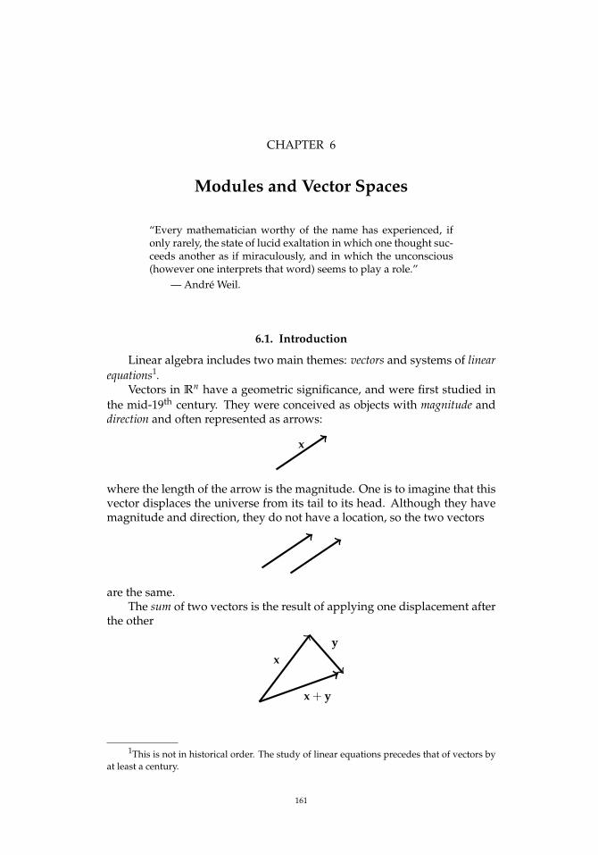
CHAPTER 6
Modules and Vector Spaces
“Every mathematician worthy of the name has experienced, ifonly rarely, the state of lucid exaltation in which one thought suc-ceeds another as if miraculously, and in which the unconscious(however one interprets that word) seems to play a role.”
— André Weil.
6.1. Introduction
Linear algebra includes two main themes: vectors and systems of linearequations1.
Vectors in Rn have a geometric significance, and were first studied inthe mid-19th century. They were conceived as objects with magnitude anddirection and often represented as arrows:
x
where the length of the arrow is the magnitude. One is to imagine that thisvector displaces the universe from its tail to its head. Although they havemagnitude and direction, they do not have a location, so the two vectors
are the same.The sum of two vectors is the result of applying one displacement after
the other
xy
x + y
1This is not in historical order. The study of linear equations precedes that of vectors byat least a century.
161
162 6. MODULES AND VECTOR SPACES
Of course, there is only so much one can do with pictures. The needto quantify vectors quickly became apparent and vectors were given a nu-merical representation, where
v =
123
represents the vector that displaces the origin to the point (1, 2, 3). Additionof vectors is easy to formulate a
bc
+
uvw
=
a + ub + vc + w
Linear equations are problems like
2x + 3y = 5
6x− y = 2(6.1.1)
where we must solve for x and y.The obstacle to solving these equations easily is that they both have
two variables. We must, somehow, isolate one of the variables — and solvefor it. Getting the second variable is straightforward.
In this case it is not hard to see that we can subtract 3× the first equationfrom the second to give
2x + 3y = 5
6x− 6x− 10y = −13(6.1.2)
so y = 13/10. Now we substitute this into the first equation to get
2x + 3 · 13/10 = 5
or x = 11/20.Mathematicians quickly developed a shorthand for a set of variables or
quantities by writing them in tables[xy
]and
[52
]called vectors, and writing the coefficients in a table
(6.1.3)[
2 36 −1
]called a matrix. Strictly speaking, a vector is a matrix with one column. Theoriginal problem is rewritten as[
2 36 −1
]·[
xy
]=
[52
]where we, somehow, define multiplication of a vector by a matrix (seeequations 6.2.6 on page 168 and 6.2.7 on page 168) in a way that reproducesequation 6.1.1.
The reader might protest that we haven’t simplified the process of solv-ing equation 6.1.1 at all. We have, however, clarified the most importantaspect of the solution: subtracting 3× the first equation from the second
6.2. VECTOR SPACES 163
only involves the coefficients — i.e. the matrix in equation 6.1.3 on the facingpage — and not the variables x and y.
We define a vector space to be the mathematical structure where vec-tors “live.”
6.2. Vector spaces
6.2.1. Basic properties. Vector-spaces and maps between them are themain objects of study of linear algebra.
DEFINITION 6.2.1. If F is a field, a vector space, V, over F is an abeliangroup with an action of F on V
•: F×V → V
— i.e. multiplication of elements of V by elements of F is well-defined. Inaddition
(1) if x ∈ F and v1, v2 ∈ V, then x · v1 + x · v2 = x · (v1 + v2),(2) if x, y ∈ F and v ∈ V, then x · v+ y · v = (x+ y) · v, and x · (y · v) =
(xy) · v,(3) 0 · v = 0 ∈ V, and 1 · v = v for all v ∈ V.
REMARK. It is easy to find examples of vector spaces: Rn is a vector space over R
C∞([0, 1]) — the set of infinitely differentiable real-valued func-tions on the interval [0, 1] — is a vector space over R.
a field is a vector space over any of its subfields. Mn,m(k) — the set of n×m matrices with entries in a field, k, is a
vector space.
DEFINITION 6.2.2. If V is a vector space over a field, k, ands = v1, . . . , vn is a set with vi ∈ V for i = 1, . . . , n then s is linearlydependent if there exists an equation
(6.2.1)n
∑i=1
αivi = 0
with αi ∈ k and at least one αi 6= 0. If s is not linearly dependent, it is saidto be linearly independent.
An infinite set of vectors is linearly independent if all of its finite subsetsare.
REMARK. If s is linearly dependent, then one of its elements is a linearcombination of the others: if αk 6= 0 in equation 6.2.1, then
vk = −α−1k
n
∑i=1,i 6=k
αivi
Note that linear independence is a property of the set of vectors that is in-herited by every subset:
A single vector is a linearly independent set if it is nonzero.Two vectors are linearly independent if neither is a multiple of the
other. This also means both of the vectors are nonzero.
164 6. MODULES AND VECTOR SPACES
DEFINITION 6.2.3. If V is a vector-space over a field k ands = v1, . . . , vn are elements of V, their span, Span(s) is the set of allpossible linear combinations
n
∑i=1
αivi
for αi ∈ k.
REMARK. It’s not hard to see that the span of a set of vectors is alwaysa vector space.
PROPOSITION 6.2.4. Let V be a vector space and let s = v1, . . . , vn be alinearly independent set of vectors. If v ∈ V and v /∈ Span(s), then the set
s ∪ vis also linearly independent.
PROOF. Suppose
αv +n
∑i=1
αivi = 0
with some nonzero coefficients (making the set s ∪ v linearly dependent).If α = 0, then we get
n
∑i=1
αivi = 0
which forces all of the αi to be zero, a contradiction. It follows that α 6= 0 sothat
v = −α−1n
∑i=1
αivi
which contradicts the hypothesis that α /∈ Span(s).
DEFINITION 6.2.5. A basis for a vector space, V, is a linearly indepen-dent set of vectors s = v1, . . . such that
V = Span(s)
Now we can outline an inductive procedure for finding a basis of avector space.
(1) Start with a nonzero vector, v1 ∈ V, and set s1 = v1,(2) In step n, sn = v1, . . . , vn. If V = Span(s), we are done and sn is
a basis. If not, there exists vn+1 ∈ V \ Span(s), and set sn+1 = sn ∪vn+1. This will be linearly independent, by proposition 6.2.4.
If this terminates in a finite number of steps, it proves a basis exists andexplicitly constructs one. Unfortunately, this is unlikely to happen in manycases — for instance if V = C∞([0, 1]).
In light of this, we have
THEOREM 6.2.6. If V is a vector-space and s = v1, . . . , vk is a linearlyindependent set of vectors, then V has a basis containing s.
6.2. VECTOR SPACES 165
PROOF. We will assume that the procedure described above never ter-minates, since we would be done in that case. Let S be the set of all linearlyindependent sets of vectors of V containing s.
We begin by claiming that every ascending chain of elements in S
A1 ⊂ A2 ⊂ · · ·has a maximum, namely
A =∞⋃
i=1
Ai
This involves proving that A = w1, . . . is a linearly independent set ofvectors, where wi = vi for i ≤ k. Any linear dependence equation
n
∑i=1
αiwi = 0
involves a finite set of vectors of A, hence would involve the vectors of Ajfor some j. This contradicts the fact that each Aj is a linearly independentset of vectors.
Zorn’s lemma ( A.2.12 on page 462) implies that S contains a maximalelement, T. This is linearly independent, and we claim that it spans V. Ifnot, there exists v ∈ V \ Span(T) and
T ∪ v ⊃ T
is linearly independent (by proposition 6.2.4 on the facing page). This con-tradicts the maximality of T.
Bases for vector spaces are interesting because they constitute coordi-nate systems:
PROPOSITION 6.2.7. If V is a vector space over a field k with a basis B =b1, . . . and v ∈ V is any vector, then there exists a unique expression
v =n
∑i=1
αibji
PROOF. We know that such an expression exists because V = Span(B).If we had two distinct expressions for v, i.e.
v =n
∑i=1
αibji =n
∑i=1
βibji
thenn
∑i=1
(αi − βi)bji = 0
and the linear independence of B implies that αi − βi = 0 for all i.
It turns out that the size of a basis is uniquely determined
PROPOSITION 6.2.8. If V is a vector space over a field k andB = b1, . . . , bn is a basis, then every other basis has precisely n elements. Thisvalue n is called the dimension of V.
166 6. MODULES AND VECTOR SPACES
REMARK. It turns out that this result is true even if the basis-sets areinfinite, but one must use transfinite induction and the axiom of choice( A.2.11 on page 461) to prove it.
PROOF. Let F = f1, . . . , fm be another basis for V.If n = 1, the fact that B is a basis implies that fi = αib1, so that
f1, . . . , fk is linearly dependent unless k = 1.Now we consider the case where n > 1.We will show that m ≤ n and the conclusion will follow by symmetry.
Since F is linearly independent, f1 6= 0. Since B is a basis, we have
(6.2.2) f1 = α1b1 + · · ·+ αnbn
Without loss of generality, assume α1 6= 0 (if necessary, rearrange the bi tomake this happen) so we can solve for b1:
(6.2.3) b1 = α−11 ( f1 − α2b2 − · · · − αnbn)
We claim that f1, b2, . . . , bn is a basis for V. If v ∈ V, there is a formula
v = β1b1 + · · ·+ βnbn
and plugging equation 6.2.3 into it gives a formula for v in terms of f1, b2, . . . , bn. It follows that f1, b2, . . . , bn spans V.
If
(6.2.4) γ1 f1 +n
∑i=2
γibi = 0
is a linear dependence relation (i.e., some of the γi 6= 0), we claim thatγ1 6= 0. If γ1 = 0, we get a linear dependence equation
n
∑i=2
γibi = 0
which contradicts the fact that B is a linearly independent set. Now weplug equation 6.2.2 into equation 6.2.4 to get
γ1 (α1b1 + · · ·+ αnbn) + γ2b2 + · · ·+ γnbn = 0
γ1α1b1 + (γ1α2 + γ2)b2 + · · ·+ (γ1αn + γn) = 0
Since we know γ1α1 6= 0, this gives a nontrivial linear dependence relationbetween the bi, a contradiction.
Assume m > n. We have established that we can replace one of the biby one of the fi and still have a basis. We do this repeatedly until we have abasis f1, . . . fn. If m > n the fi with i > n will be linear combinations of f1, . . . fn and the original set f1, . . . , fm cannot be linearly independent:a contradiction.
It follows that m ≤ n and symmetry (i.e., starting with the F-basis andsuccessively replacing basis elements by the bi) shows that n ≤ m, so theyare equal.
DEFINITION 6.2.9. If a vector-space V over field k has a finite basisB = b1, . . . , bn and
v =n
∑i=1
αibi
6.2. VECTOR SPACES 167
is the unique expression for v ∈ V, we use the notation
(6.2.5) v =
α1...
αn
B
which we will call a matrix with one column and n rows.
REMARK. Note that the elements αi in equation 6.2.5 depend on thebasis used to compute them.
6.2.2. Linear transformations. Having defined vector spaces, we turnto the question of maps between them:
DEFINITION 6.2.10. If V1 and V2 are vector spaces over the field k, ahomomorphism or linear transformation
f : V1 → V2
is a function with the properties(1) for all v, w ∈ V1, we have f (v + w) = f (v) + f (w)(2) for all v ∈ V1, x ∈ k, we have f (x · v) = x · f (v)
The set of vectors v ∈ V1with the property that f (v) = 0 is called thenullspace of f , denoted Null( f ).
REMARK. The nullspace is just the kernel of f , regarded as a map ofabelian groups (for instance). It is clearly a subspace of V1.
Suppose we have a linear transformation
f : V →W
and B = b1, . . . , bn is a basis for B and G = g1, . . . , gm is a basis for W.If v ∈ V is given by
v =n
∑i=1
αibi
then the definition of a linear transformation implies that
f (v) =n
∑i=1
αi f (bi)
If
f (bi) =
β1,i...
βn,i
G
then
f (v) =
β1,1 · · · β1,n...
. . ....
βm,1 · · · βm,n
α1
...αn
in the G-basis. The quantity
M =
β1,1 · · · β1,n...
. . ....
βm,1 · · · βm,n
168 6. MODULES AND VECTOR SPACES
is called an n×m matrix, and the product is defined by
(6.2.6)
β1,1 · · · β1,n...
. . ....
βm,1 · · · βm,n
α1
...αn
= α1
β1,1...
βm,1
+ · · ·+ αn
β1,n...
βm,n
or, if we regard the columns of M as m× 1 matrices, so
(6.2.7) M =[
C1 · · · Cn]
where the Ci are called column-vectors of M, we get
f (v) =n
∑i=1
αiCi
or
f (v)i =n
∑j=1
βi,jαj
so that a matrix is a convenient notation for representing a linear transfor-mation. We will also use the notation
(6.2.8) M =
R1...
Rm
where the Ri are the rows of M, regarded as 1× n matrices.
By abuse of notation, we will often refer to the nullspace (see defini-tion 6.2.10 on the preceding page) of a matrix.
Note that the matrix-representation of a linear transformation dependsin a crucial way on the bases used.
DEFINITION 6.2.11. If n ≥ 1 is an integer, define the identity matrix
In =
1 0 · · · 00 1 · · · 0
0 0. . .
...0 0 · · · 1
or
Ii,j =
1 if i = j0 otherwise
REMARK. It is not hard to see that
In
α1...
αn
=
α1...
αn
which motivates the term identity matrix. It represents the identity mapregarded as a linear transformation.
DEFINITION 6.2.12. If A is an n×m matrix, its transpose, At is an m× nmatrix defined by
(Ati,j) = Aj,i
6.2. VECTOR SPACES 169
Composites of linear transformations give rise to matrix products:
DEFINITION 6.2.13. If A is an n × m matrix and B is an m × k matrixwith
B =[
C1 · · · Ck]
where the Ci are the column-vectors, then
AB =[
AC1 · · · ACk]
or
(AB)i,j =m
∑`=1
Ai,`B`,j
— an n× k matrix. If A and B are n× n matrices and AB = I, A is said tobe invertible and B is its inverse.
Note that any isomorphism of vector spaces is represented by a squarematrix since the size of a basis is uniquely determined.
EXERCISES.
1. Which of the following functions define linear transformations?
a. f (x, y, z) = xy + zb. f (x, y, z) = 3x + 2y− zc. f (x, y, z) = x + y + z + 1d. f (x, y, z) = z− x + 5
2. Show that matrix-multiplication is distributive over addition andassociative, so that the set of all n× n matrices over a ring, R, forms a (non-commutative) ring Mn(R).
3. Show that powers of a matrix commute with each other, i.e. for anymatrix, A, over a ring, R, and any n, m ≥ 0, show that
An · Am = Am · An
4. If R is a commutative ring, Mn(R) is the ring of n × nmatrices, and A ∈ Mn(R) is a specific matrix, show that there exists aring-homomorphism
R[X]→ Mn(R)X 7→ A
so that the matrix A generates a commutative subring R[A] ⊂ Mn(R).
170 6. MODULES AND VECTOR SPACES
6.2.3. Determinants.
DEFINITION 6.2.14. If M is an n× n matrix, its determinant, det(M) isdefined by
(6.2.9) det(M) = ∑σ∈Sn
℘(σ)M1,σ(1) · · ·Mn,σ(n)
where the sum is taken over all n! permutations in Sn. If τ ∈ Sn is anytransposition and An C Sn is the alternating group (see definition 4.5.10 onpage 54), then τ projects to the nontrivial element of Sn/An = Z2 so
Sn = An t τ · An
as sets. We can rewrite formula 6.2.9 as
det(M) = ∑σ∈An
M1,σ(1) · · ·Mn,σ(n) − ∑σ∈An
M1,τσ(1) · · ·Mn,τσ(n)(6.2.10)
= ∑σ∈An
(M1,σ(1) · · ·Mn,σ(n) −M1,τσ(1) · · ·Mn,τσ(n)
)(6.2.11)
since all the permutations in An are even.
REMARK. Equation 6.2.9 is due to Euler. It is not particularly suited tocomputation of the determinant since it is a sum of n! terms.
In a few simple cases, one can write out the determinant explicitly:
(6.2.12) det[
a bc d
]= ad− bc
and
det
a11 a12 a13a21 a22 a23a31 a32 a33
= a11a22a33 + a11a23a31 + a13a32a21(6.2.13)
− a13a22a31 − a23a32a11 − a33a21a12
DEFINITION 6.2.15. An n × n matrix, A, is called upper-triangularifAi,j = 0 whenever i > j. The matrix, A, is lower triangular if Ai,j = 0whenever j > i.
REMARK. The term “upper-triangular” comes from the fact that Alooks like
A1,1 A1,2 · · · A1,n−1 A1,n
0 A2,2. . . A2,n−1 A2,n
0 0. . .
......
......
. . . An−1,n−1 An−1,n0 0 · · · 0 An,n
We explore a closely related concept:
DEFINITION 6.2.16. Let A be an n× n upper-triangular matrix. In anygiven row, the pivot element is the first nonzero entry encountered, scanningfrom left to right. Suppose the pivot element in row i is Ai,p(i), so that the
6.2. VECTOR SPACES 171
pivot-column for row i is p(i). We define the matrix A to be in echelon formif
(1) p(j) > p(i) whenever j > i.(2) rows of all zeroes lie below rows that have nonzero entries
REMARK. Oddly enough, the term echelon form comes from the mili-tary, referring to a formation of soldiers. Here’s an example of a matrix inechelon form
2 0 1 0 30 1 0 4 00 0 0 1 50 0 0 0 30 0 0 0 0
with its pivots highlighted. The point of echelon form is that the pivotelement in every row is to the right of the pivots in the rows above it.
Here’s an example of a upper-triangular matrix that is not in echelonform
2 0 1 0 30 1 0 4 00 0 0 1 50 0 0 0 30 0 0 0 2
The problem is that it has two pivots in the same column. Another exampleof an upper-triangular matrix that is not echelon is
2 0 1 0 30 0 0 0 00 0 2 1 50 0 0 7 30 0 0 0 2
Here, the problem is that there is a row of zeroes above rows that havenonzero entries.
In the next few results we will investigate the properties of determi-nants.
PROPOSITION 6.2.17. If M is an n× n matrix, then
det(Mt) = det(M)
PROOF. Definitions 6.2.14 on the facing page and 6.2.12 on page 168imply that
det(Mt) = ∑σ∈Sn
℘(σ)Mσ(1),1 · · ·Mσ(n),n
= ∑σ∈Sn
℘(σ)M1,σ−1(1) · · ·Mn,σ−1(n) sorting by left subscripts
= ∑σ∈Sn
℘(σ−1)M1,σ−1(1) · · ·Mn,σ−1(n) since ℘(σ−1) = ℘(σ)
= det(M)
172 6. MODULES AND VECTOR SPACES
since, if σ runs over all permutations in Sn, so does σ−1.
PROPOSITION 6.2.18. If M is an n× n upper- or lower-triangular matrix
det M =n
∏i=1
Mi,i
PROOF. We’ll do the upper-triangular case — the other case followsfrom proposition 6.2.17 on the preceding page. In equation 6.2.9 onpage 170, all terms with σ(i) < i will have a factor of 0, so we must haveσ(i) ≥ i for all i. For all permutations, σ
n
∑i=1
(i− σ(i)) = 0
If σ 6= 1, some terms will have (j − σ(j)) > 0 and must be balanced byother terms (j′ − σ(j′)) < 0. If follows that σ(i) ≥ i for all i implies that σis the identity.
COROLLARY 6.2.19. If M is an n× n matrix in echelon form and det M =0, then the bottom row of M consists of zeros.
PROOF. Since det M = 0, proposition 6.2.15 on page 170implies thatone of the diagonal entries of M is 0. This implies that there is a pivotelement ≥ 2 columns to the right of the pivot of the previous row. Since Mhas the same number of rows and columns, the pivot elements must reachthe right side of M before they reach the bottom, so the bottom row consistsof zeroes.
PROPOSITION 6.2.20. If M is an n× n matrix and M′ is the result of inter-changing rows i and j 6= i or columns i and j of M, then
det M′ = −det M
PROOF. We will prove this for interchanged columns; the conclusionfor interchanged rows follows from 6.2.17 on the previous page.
Let τ = (i, j), the transposition. Then equation 6.2.10 on page 170 (andthe fact that τ2 = 1)implies that
det(M′) = ∑σ∈An
M′1,σ(1) · · ·M′n,σ(n) − ∑σ∈An
M′1,τσ(1) · · ·M′n,τσ(n)
= ∑σ∈An
M1,τσ(1) · · ·Mn,τσ(n) − ∑σ∈An
M1,σ(1) · · ·Mn,σ(n)
= −det(M)
We have the related result:
PROPOSITION 6.2.21. If M is an n× n matrix and M has two rows or twocolumns that are the same, then det(M) = 0.
REMARK. If we are working over an integral domain whose character-istic is 6= 2, this follows immediately from proposition 6.2.20 since it showsthat det(M) = −det(M).
6.2. VECTOR SPACES 173
PROOF. We’ll suppose columns i and j 6= i are identical; the corre-sponding result for rows follows from proposition 6.2.17 on page 171.
Let τ ∈ Sn be the transposition (i, j). Then
M1,σ(1) · · ·Mn,σ(n) = M1,τσ(1) · · ·Mn,τσ(n)
for all σ ∈ An and equation 6.2.10 on page 170 implies that
det(M) = ∑σ∈An
(M1,σ(1) · · ·Mn,σ(n) −M1,τσ(1) · · ·Mn,τσ(n)
)= 0
The next two results follow immediately from equation 6.2.9 onpage 170; their proofs are left as exercises for the reader.
PROPOSITION 6.2.22. If
A =
R1...
Ri...
Rn
is an n× n matrix and
B =
R1...
k · Ri...
Rn
where k is a constant, then det B = k · det A.
PROPOSITION 6.2.23. If
A =
R1...
Ri−1Ri
Ri+1...
Rn
and B =
R1...
Ri−1Si
Ri+1...
Rn

174 6. MODULES AND VECTOR SPACES
are n× n matrices and
C =
R1...
Ri−1Ri + Si
Ri+1...
Rn
then
det C = det A + det B
DEFINITION 6.2.24. If A is an m × n matrix, the act of adding a mul-tiple of one row to another is called a type 1 elementary row operation. If Imis an m × m identity matrix, the result of performing an elementary rowoperation on Im is called an type 1 elementary matrix.
REMARK 6.2.25. It is not hard to see that performing a type 1 elemen-tary row operation on A is the same as forming the product EA, where E isan m×m type 1 elementary matrix.
There are type 2 and three elementary row operations, too:
Type 2: involves swapping two rows of a matrixType 3: involves multiplying a row of a matrix by a nonzero constant.
PROPOSITION 6.2.26. Elementary matrices are invertible and their inversesare other elementary matrices.
REMARK. For instance 1 0 00 1 0α 0 1
· 1 0 0
0 1 0−α 0 1
=
1 0 00 1 00 0 1
PROOF. The inverse of adding α× row i to row j is adding −α× row i
to row j.
COROLLARY 6.2.27. If A is an n × n matrix and we perform a type 1 ele-mentary row operation on A, the determinant is unchanged.
PROOF. Suppose we add a multiple of row i to row k with j > i andsuppose
A =
R1...
Ri...
Rj...
Rn
, B =
R1...
Ri...
Ri...
Rn
, C =
R1...
Ri...
k · Ri...
Rn
and D =
R1...
Ri...
k · Ri + Rj...
Rn
6.2. VECTOR SPACES 175
where k is a constant. Then det C = 0, by corollary 6.2.21 on page 172 andproposition 6.2.22 on page 173. Proposition 6.2.23 on page 173 implies that
det D = det A + det C = det A
Proposition 6.2.17 on page 171, coupled with these results, immediatelyimplies
PROPOSITION 6.2.28. Let A = [ C1 · · · Cn ] be an n× n matrix withcolumn-vectors Ci.
(1) if Ci = Cj for i 6= j, then det A = 0,(2) if A′ =
[C1 · · · Ci−1 k · Ci Ci+1 · · · Cn
]— the ith column
has been multiplied by a constant k — then
det A′ = k · det A
(3) IfB =
[C1 · · · Ci−1 Di Ci+1 · · · Cn
]and
C =[
C1 · · · Ci−1 Ci + Di Ci+1 · · · Cn]
— i.e., their columns are the same as those of A except for the ith — thendet C = det A + det B
This leads to an application for determinants2:
THEOREM 6.2.29 (Cramer’s Rule). Let
A = [ C1 · · · Cn ] =
A1,1 · · · A1,n...
. . ....
An,1 · · · An,n
, and B =
b1...
bn
and let Ai =
[C1 · · · Ci−1 B Ci+1 · · · Cn
]— the result of replacing
the ith column of A by B. If
A1,1x1 + · · ·+ A1,nxn = b1
...An,1x1 + · · ·+ An,nxn = bn(6.2.14)
is a system of linear equations, then
(6.2.15) (det A) · xi = det Ai
If det A 6= 0, then
xi =det Aidet A
REMARK. Note that we have not used the fact that we are working overa field until the last step. It follows that equation 6.2.15 is valid over anycommutative ring. This is used in a proof of the Cayley-Hamilton Theorem( 6.2.57 on page 197) in Example 6.3.18 on page 227.
2The reader has, no doubt, wondered what they are “good for.”
176 6. MODULES AND VECTOR SPACES
PROOF. Just plug both sides of equation 6.2.14 on the preceding pageinto the ith column of A and take determinants. If
E =
A1,1x1 + · · ·+ A1,nxn...
An,1x1 + · · ·+ An,nxn
then equations 6.2.14 on the previous page become
(6.2.16) det[
C1 · · · Ci−1 E Ci+1 · · · Cn]= det Ai
On the other hand
(6.2.17) det[
C1 · · · Ci−1 E Ci+1 · · · Cn]
= det[
C1 · · · Ci−1 x1 · C1 Ci+1 · · · Cn]+
· · ·+ det[
C1 · · · Ci−1 xi · Ci Ci+1 · · · Cn]+
· · ·+ det[
C1 · · · Ci−1 xn · Cn Ci+1 · · · Cn]
= x1 · det[
C1 · · · Ci−1 C1 Ci+1 · · · Cn]+
· · ·+ xi · det[
C1 · · · Ci−1 Ci Ci+1 · · · Cn]+
· · ·+ xn · det[
C1 · · · Ci−1 Cn Ci+1 · · · Cn]
Now, note that
det[
C1 · · · Ci−1 Cj Ci+1 · · · Cn]
=
det A if i = j0 if i 6= j because column j is duplicated
Plugging this into equation 6.2.17 gives
det[
C1 · · · Ci−1 E Ci+1 · · · Cn]= xi · det A
and equation 6.2.15 on the previous page follows.
Gabriel Cramer (1704-1752), was a Swiss mathematician born in Genevawho worked in geometry and analysis. Cramer used his rule in the book,[25], to solve a system of five equations in five unknowns. The rule hadbeen used before by other mathematicians. Although Cramer’s Rule is notthe most efficient method of solving systems of equations, it has theoreticapplications.
We can develop an efficient algorithm for computing determinants us-ing propositions 6.2.27 on page 174 and 6.2.20 on page 172:
PROPOSITION 6.2.30 (Gaussian Elimination). If A is an n × n matrix,the following algorithm computes an echelon matrix, A, with d · det A = det A(where d is defined below):
d← 1c← 1for r = 1, . . . , n− 2 do . Main for-loop
if Ar,i = 0 for all c ≤ i ≤ n thenMove row r to the last row . This is a row of zeroes.

6.2. VECTOR SPACES 177
end ifif Ar,c = 0 then
if ∃ row k with r ≤ k ≤ n and Ak,c 6= 0 thenSwap row r with row kd← −d
elsec← c + 1 . The new pivot is more than one column
. further to the rightPerform next iteration of the Main for-loop
end ifend iffor i = r + 1, . . . , n do . For all lower rows
for j = c, . . . , n do . do an type 1 elementary row-operationAi,j ← Ai,j − Ai,c
Ar,c· Ar,j
end forend forc← c + 1 . Advance the pivot-column
end for
REMARK. This algorithm is reasonably fast (proportional to n3 stepsrather than n!) and can easily be turned into a computer program.
This algorithm first appeared in Europe in the notes of Isaac Newton.In the 1950’s it was named after Gauss due to confusion about its history.Forms of it (with no proofs) appeared in Chapter 8: Rectangular Arrays ofthe ancient Chinese treatise, The Nine Chapters on the Mathematical Art (see[26]).
PROOF. The variable d keeps track of how many times we swap rows— because proposition 6.2.20 on page 172 implies that each such swapmultiplies the determinant by −1. The only other thing we do with A iselementary row operations, which leave the determinant unchanged bycorollary 6.2.27 on page 174. In the end, the matrix is echelon and proposi-tion 6.2.18 on page 172 implies that the determinant is the product of diag-onal entries.
Here are some examples:Start with
A =
1 2 0 6 31 1 1 0 22 0 1 2 30 5 1 1 11 3 0 5 1
The first pivot column is 1 and we start with the first row. We subtract thefirst row from the second, 2× the first row from the third and the first row
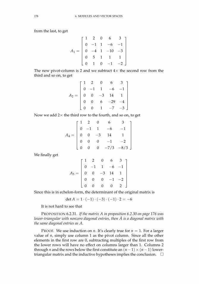
178 6. MODULES AND VECTOR SPACES
from the last, to get
A1 =
1 2 0 6 3
0 −1 1 −6 −1
0 −4 1 −10 −3
0 5 1 1 1
0 1 0 −1 −2
The new pivot-column is 2 and we subtract 4× the second row from thethird and so on, to get
A2 =
1 2 0 6 3
0 −1 1 −6 −1
0 0 −3 14 1
0 0 6 −29 −4
0 0 1 −7 −3
Now we add 2× the third row to the fourth, and so on, to get
A4 =
1 2 0 6 3
0 −1 1 −6 −1
0 0 −3 14 1
0 0 0 −1 −2
0 0 0 −7/3 −8/3
We finally get
A5 =
1 2 0 6 3
0 −1 1 −6 −1
0 0 −3 14 1
0 0 0 −1 −2
0 0 0 0 2
Since this is in echelon-form, the determinant of the original matrix is
det A = 1 · (−1) · (−3) · (−1) · 2 = −6
It is not hard to see that
PROPOSITION 6.2.31. If the matrix A in proposition 6.2.30 on page 176 waslower-triangular with nonzero diagonal entries, then A is a diagonal matrix withthe same diagonal entries as A.
PROOF. We use induction on n. It’s clearly true for n = 1. For a largervalue of n, simply use column 1 as the pivot column. Since all the otherelements in the first row are 0, subtracting multiples of the first row fromthe lower rows will have no effect on columns larger than 1. Columns 2through n and the rows below the first constitute an (n− 1)× (n− 1) lower-triangular matrix and the inductive hypotheses implies the conclusion.
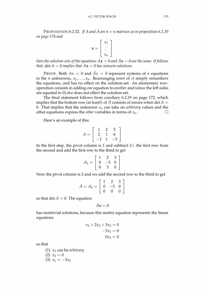
6.2. VECTOR SPACES 179
PROPOSITION 6.2.32. If A and A are n× n matrices as in proposition 6.2.30on page 176 and
x =
x1...
xn
then the solution-sets of the equations Ax = 0 and Ax = 0 are the same. It followsthat, det A = 0 implies that Ax = 0 has nonzero solutions.
PROOF. Both Ax = 0 and Ax = 0 represent systems of n equationsin the n unknowns, x1, . . . , xn. Rearranging rows of A simply renumbersthe equations, and has no effect on the solution-set. An elementary row-operation consists in adding one equation to another and (since the left sidesare equated to 0) also does not effect the solution-set.
The final statement follows from corollary 6.2.19 on page 172, whichimplies that the bottom row (at least!) of A consists of zeroes when det A =0. That implies that the unknown xn can take on arbitrary values and theother equations express the other variables in terms of xn.
Here’s an example of this:
A =
1 2 32 1 6−1 1 −3
In the first step, the pivot column is 1 and subtract 2× the first row fromthe second and add the first row to the third to get
A1 =
1 2 30 −3 00 3 0
Now the pivot column is 2 and we add the second row to the third to get
A = A2 =
1 2 30 −3 00 0 0
so that det A = 0. The equation
Ax = 0
has nontrivial solutions, because this matrix equation represents the linearequations
x1 + 2x2 + 3x3 = 0−3x2 = 0
0x3 = 0
so that(1) x3 can be arbitrary(2) x2 = 0(3) x1 = −3x3
180 6. MODULES AND VECTOR SPACES
and the general solution can be written as
x = x3
−301
It is easy to check that Ax = 0, so that equation has nonzero solutions (aninfinite number of them, in fact).
COROLLARY 6.2.33. If A is an n× n matrix, the following statements areequivalent:
(1) det A 6= 0(2) if
x =
x1...
xn
the equation Ax = 0 has x = 0 as its only solution.
(3) the rows of A are linearly independent,(4) the columns of A are linearly independent(5) A has an inverse
PROOF. Cramer’s Rule (theorem 6.2.29 on page 175) also implies thatAx = 0 has x = 0 as its only solution.
SupposeA =
[C1 · · · Cn
]and
α1C + · · ·+ αnCn = 0is a linear dependence equation. If det A 6= 0, then theorem 6.2.29 onpage 175 implies
α1 = · · · = αn = 0so the columns of A are linearly independent.
Taking the transpose of A and invoking proposition 6.2.17 on page 171implies that the rows are linearly independent.
Now suppose det A = 0. Then proposition 6.2.32 on the previous pageimplies that the equation Ax = 0 has nontrivial solutions and
Ax = x1C1 + · · ·+ xnCn = 0
is a nontrivial dependence relation between columns. Since A annihilatesnonzero vectors (the nontrivial solutions of Ax = 0) it cannot have an in-verse (even as a function). Cramer’s Rule (theorem 6.2.29 on page 175) im-plies that the equations
Axi =
0...010...0
6.2. VECTOR SPACES 181
have unique solutions, where the 1 on the right occurs in the ith row. Thematrix [
x1 · · · xn]
is easily seen to be A−1.
This, remark 6.2.25 on page 174, and proposition 6.2.26 on page 174imply that:
COROLLARY 6.2.34. If A is an n× n matrix, there exists an equation
S1 · · · Sk · A = U
where the Si are either lower triangular elementary matrices or transpositions andU is upper-triangular. It follows that
(6.2.18) A = Tn · · · T1 ·Uwhere Ti = S−1
i are also lower triangular elementary matrices. We also have adecomposition
A = L · R1 · · · Rk
where L is lower-triangular and the Ri are upper-triangular elementary matricesor transpositions. If det A 6= 0, we have a decomposition
(6.2.19) A = Tn · · · T1 · D · R1 · · · Rk
where D is a diagonal matrix.
PROOF. To prove the second statement, simply take the transpose of Aand apply equation 6.2.18:
At = Tk · · · T1 ·Uand take the transpose
A = Ut · Tt1 · · · Tt
kThe transpose of an upper-triangular matrix is lower-triangular and thetranspose of an elementary matrix is elementary.
The final statement follows from proposition 6.2.31 on page 178, ap-plied to L.
The determinant has an interesting property:
THEOREM 6.2.35. If A and B are n× n matrices, then
det(AB) = det A · det B
PROOF. We divide this into cases.(1) det B = 0. In this case, the equation Bx = 0 has nontrivial solu-
tions, by proposition 6.2.32 on page 179. It follows that ABx = 0 aswell, and corollary 6.2.33 on the facing page implies that det AB =0.
(2) From now on, det B 6= 0. If B is an elementary matrix, det B = 1.We have (AB)t = Bt At and Bt At is the result of performing an el-ementary row operation on At so corollary 6.2.27 on page 174 im-plies that det Bt At = det At. Since proposition 6.2.17 on page 171implies that det M = det Mt for any n × n matrix, M, it followsthat det AB = det A and the conclusion follows.
182 6. MODULES AND VECTOR SPACES
(3) In this case, use corollary 6.2.34 on the previous page to representB via
B = Tn · · · T1 · D · R1 · · · Rk
and the T’s and R’s are elementary matrices. The productof the diagonal entries in D give the determinant of B,i.e.det B = ∏n
i=1 Di,i. Then
det(AB) = det(A · Tn · · · T1 · D · R1 · · · Rk)
= det(A′ · D) where det A′ = det A
= det A′ · det B= det A · det B
since A′D is the result of multiplying row i of A′ by Di,i and eachsuch multiplication multiplies det A′ = det A by Di,i, by proposi-tion 6.2.23 on page 173.
DEFINITION 6.2.36. If A is an n× n matrix and 1 ≤ i, j ≤ n, then the(i, j)th minor of A, denoted Mi,j(A) is the determinant of the (n− 1)× (n−1) matrix formed from A by deleting its ith row and its jth column.
The use of minors leads to another way to compute determinants:
PROPOSITION 6.2.37. If A is an n × n matrix, and k = 1, . . . , n is fixed,then
det A =n
∑i=1
(−1)i+j Ak,i ·Mk,i(A)(6.2.20)
Furthermore, if j 6= k , we have
Aj,1 ·Mk,1(A)− Aj,2 ·Mk,2(A) + · · ·+ (−1)n+1 Aj,n ·Mk,n(A) = 0
PROOF. We begin by proving the claim for k = 1. Recall the equationof the determinant
(6.2.21) det(A) = ∑σ∈Sn
℘(σ)A1,σ(1) · · · An,σ(n)
Now note that A1,i · M1,i(A) is all terms of equation 6.2.21 for whichσ(1) = i and
M1,i(A) = ∑τ∈Sn−1
℘(τ)A2, f (τ(1)) · · · An, f (τ(n−1))
where
f (k) =
k if k < ik + 1 if k ≥ i
Write τ′ = τ, extended to Sn by setting τ′(n) = n. Then ℘(τ′) = ℘(τ).Converting from τ′ to σ involves
(1) decreasing all indices by 1 and mapping 1 to n (which τ′ fixes)(2) applying τ′
(3) increasing all indices ≥ i by 1 and mapping n to i

6.2. VECTOR SPACES 183
In other words
σ = (i, i + 1, . . . , n) τ′ (n, . . . , 1)
which implies that
℘(τ′) = (−1)(n+1)+(n−i)℘(σ) = (−1)2n+i+1℘(σ) = (−1)i+1℘(σ)
The sum of all the terms of equation 6.2.20 on the facing page accounts forall of the terms in equation 6.2.21 on the preceding page.
The statement for k 6= 1 follows from constructing a matrix, V, via
V =
Ak,1 · · · Ak,nA1,1 · · · A1,n
.... . .
...Ak−1,1 · · · Ak−1,nAk+1,1 · · · Ak+1,n
.... . .
...An,1 · · · An,n
where the kth row has been “shuffled” to the top via k − 1 swaps of rows— in other words, the kth row has been moved to the top in a way thatpreserves the relative order of the other rows. It follows that
det V = (−1)k+1 det A
and the conclusion follows from the fact that M1,i(V) = Mk,i(A), V1,i = Ak,ifor i = 1, . . . , n.
The final statement follows from the fact that we are computing thedeterminant of a matrix whose jth and kth rows are the same.
We can define the adjoint or adjugate of a matrix:
DEFINITION 6.2.38. If A is an n × n matrix, we define the adjoint oradjugate of A, denoted adj(A) via
adj(A)i,j = (−1)i+j Mj,i(A)
Proposition 6.2.37 on the facing page immediately implies that
PROPOSITION 6.2.39. If A is an n× n matrix
A · adj(A) = det A · Iwhere I is the n× n identity matrix. If det A 6= 0, we get
A−1 =1
det A· adj(A)
REMARK. Note that A commutes with its adjugate because the latter isa scalar multiple of the inverse of A.

184 6. MODULES AND VECTOR SPACES
6.2.4. Application of determinants: Resultants of polynomials. Resultants ofpolynomials answer many of the same questions as Gröbner bases, but are compu-tationally more tractable.
We begin by trying to answer the question:Given polynomials
f (x) = anxn + · · ·+ a0(6.2.22)g(x) = bmxm + · · ·+ b0(6.2.23)
when do they have a common root?An initial (but not very helpful) answer is provided by:
LEMMA 6.2.40. If f (x) is a nonzero degree n polynomial and g(x) is a nonzero de-gree m polynomial, they have a common root if and only if there exist nonzero polynomialsr(x) of degree ≤ m− 1 and s(x) of degree ≤ n− 1 such that
(6.2.24) r(x) f (x) + s(x)g(x) = 0
REMARK. Note that the conditions on the degrees of r(x) and s(x) are impor-tant. Without them, we could just write
r(x) = g(x)s(x) = − f (x)
and always satisfy equation 6.2.24.
PROOF. Suppose f (x), g(x) have a common root, α. Then we can set
r(x) = g(x)/(x− α)
s(x) = − f (x)/(x− α)
and satisfy equation 6.2.24.On the other hand, if equation 6.2.24 is satisfied it follows that r(x) f (x) and
s(x)g(x) are degree t ≤ n + m− 1 polynomials that have the same t factors
x− α1, . . . , x− αt
since they cancel each other out. This set (of factors) of size t includes the n factorsof f (x) and the m factors of g(x). The pigeonhole principal implies that at least 1 ofthese factors must be common to f (x) and g(x). And this common factor impliesthe existence of a common root.
Suppose
r(x) = um−1xm−1 + · · ·+ u0
s(x) = vn−1xn−1 + · · ·+ v0
Then
r(x) · f (x) =n+m−1
∑i=0
xici(6.2.25)
s(x) · g(x) =n+m−1
∑i=0
xidi
where ci = ∑j+k=i ujak. We can compute the coefficients ci by matrix products
[um−1, . . . , u0]
an0...0
= cn+m−1

6.2. VECTOR SPACES 185
and
[um−1, . . . , u0]
an−1
an0...0
= cn+m−2
or, combining the two,
[um−1, . . . , u0]
an an−10 an0 0...
...0 0
= [cn+m−1, cn+m−2]
where the subscripts of ak increase from top to bottom and those of the uj increasefrom left to right.
On the other end of the scale
[um−1, . . . , u0]
0...0a0
= c0
and
[um−1, . . . , u0]
0...0a0a1
= c1
so we get
[um−1, . . . , u0]
0 0...
...0 0a0 0a1 a0
= [c1, c0]
This suggests creating a matrix
M1 =
an an−1 · · · a0 0 · · · 0
0 an · · · a1. . . · · · 0
.... . .
. . ....
. . .. . .
...0 · · · 0 an · · · a1 a0
of m rows and n + m columns. The top row contains the coefficients of f (x) fol-lowed by m− 1 zeros and each successive row is the one above shifted to the right.We stop when a0 reaches the rightmost column. Then[
um−1 · · · u0]
M1 =[
cn+m−1 · · · c0]= [c]
186 6. MODULES AND VECTOR SPACES
so we get the coefficients of r(x) f (x). In like fashion, we can define a matrix with nrows and n + m columns
M2 =
bm bm−1 · · · b0 0 · · · 0
0 bm · · · b1. . . · · · 0
.... . .
. . ....
. . .. . .
...0 · · · 0 bm · · · b1 b0
whose top row is the coefficients of g(x) followed by n− 1 zeros and each successiverow is shifted one position to the right, with b0 on the right in the bottom row. Then[
vn−1 · · · v0]
M2 = [dn+m−1, . . . , d0] = [d]
— a vector of the coefficients of s(x)g(x). If we combine the two together, we getan (n + m)× (n + m)-matrix
S =
[M1M2
]with the property that
(6.2.26)[
u v]
S = [c + d]
— an n + m dimensional vector of the coefficients of r(x) f (x) + s(x)g(x), where
u =[
um−1 · · · u0]
(6.2.27)
v =[
vn−1 · · · v0]
It follows that S reduces the question of the existence of a common root of f (x)and g(x) to linear algebra: The equation
(6.2.28)[
u v]
S = [0]
has a nontrivial solution if and only if det(S) = 0 by corollary 6.2.33 on page 180.
DEFINITION 6.2.41. If
f (x) = anxn + · · ·+ a0
g(x) = bmxm + · · ·+ b0
are two polynomials, their Sylvester Matrix is the (n + m)× (n + m)-matrix
S( f , g, x) =
an an−1 · · · a0 0 · · · 0
0 an · · · a1. . . · · · 0
.... . .
. . ....
. . .. . .
...0 · · · 0 an · · · a1 a0
bm bm−1 · · · b0 0 · · · 0
0 bm · · · b1. . . · · · 0
.... . .
. . ....
. . .. . .
...0 · · · 0 bm · · · b1 b0
and its determinant det(S( f , g, x)) = Res( f , g, x) is called the resultant of f and g.
James Joseph Sylvester (1814–1897) was an English mathematician whomade important contributions to matrix theory, invariant theory, numbertheory and other fields.
The reasoning above shows that:

6.2. VECTOR SPACES 187
PROPOSITION 6.2.42. The polynomials f (x) and g(x) have a common root if andonly if Res( f , g, x) = 0.
PROOF. Equations 6.2.23 on page 184 and 6.2.26 on the facing page implythat the hypothesis of lemma 6.2.40 on page 184 is satisfied if and only ifdet(S( f , g, x)) = 0.
EXAMPLE. For instance, suppose
f (x) = x2 − 2x + 5
g(x) = x3 + x− 3
Then the Sylvester matrix is
M =
1 −2 5 0 00 1 −2 5 00 0 1 −2 51 0 1 −3 00 1 0 1 −3
and the resultant is 169, so these two polynomials have no common roots.
There are many interesting applications of the resultant. Suppose we are givenparametric equations for a curve
x =f1(t)g1(t)
y =f2(t)g2(t)
where fi and gi are polynomials, and want an implicit equation for that curve, i.e.one of the form
F(x, y) = 0
This is equivalent to finding x, y such that the polynomials
f1(t)− xg1(t) = 0f2(t)− yg2(t) = 0
have a common root (in t). So the condition is
Res( f1(t)− xg1(t), f2(t)− yg2(t), t) = 0
This resultant will be a polynomial in x and y. We have eliminated the variable t —in a direct generalization of Gaussian elimination (see 6.2.30 on page 176) — andthe study of such algebraic techniques is the basis of Elimination Theory.
For example, let
x = t2
y = t2(t + 1)
Then the Sylvester matrix is
1 0 −x 0 0
0 1 0 −x 0
0 0 1 0 −x
1 1 0 −y 0
0 1 1 0 −y
188 6. MODULES AND VECTOR SPACES
and the resultant is
Res(t2 − x, t2(t + 1)− y, t) = −x3 + y2 − 2 yx + x2
and it is not hard to verify that
−x3 + y2 − 2 yx + x2 = 0
after plugging in the parametric equations for x and y.
EXERCISES.
5. Compute an implicit equation for the curve defined parametrically by
x = t/(1 + t2)
y = t2/(1− t)
6. Compute an implicit equation for the curve
x = t/(1− t2)
y = t/(1 + t2)
7. Compute an implicit equation for the curve
x = (1− t)/(1 + t)
y = t2/(1 + t2)
8. Solve the equations
x2 + y2 = 1
x + 2y− y2 = 1
by computing a suitable resultant to eliminate y.
9. Find implicit equations for x, y, and z if
x = s + ty = s2 − t2
z = 2s− 3t2
Hint: Compute resultants to eliminate s from every pair of equations and then elim-inate t from the resultants.
6.2.5. A geometric property of determinants. Consider the effect ofoperating on the unit cube, [0, 1]n, in Rn via a matrix. In R2 the unit squareat the origin becomes a parallelogram, as in figure 6.2.1 on the next page
We give a heuristic argument that an elementary matrix does not alterthe n-dimensional volume of a region of Rn:
PROPOSITION 6.2.43. In R2, an elementary matrix leaves the area of thesquare [x, x + 1]× [y, y + 1] unchanged.
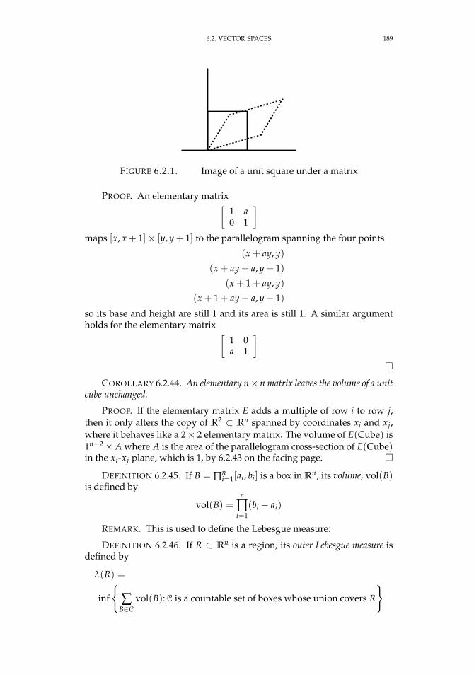
6.2. VECTOR SPACES 189
FIGURE 6.2.1. Image of a unit square under a matrix
PROOF. An elementary matrix[1 a0 1
]maps [x, x + 1]× [y, y + 1] to the parallelogram spanning the four points
(x + ay, y)
(x + ay + a, y + 1)
(x + 1 + ay, y)
(x + 1 + ay + a, y + 1)
so its base and height are still 1 and its area is still 1. A similar argumentholds for the elementary matrix [
1 0a 1
]
COROLLARY 6.2.44. An elementary n× n matrix leaves the volume of a unitcube unchanged.
PROOF. If the elementary matrix E adds a multiple of row i to row j,then it only alters the copy of R2 ⊂ Rn spanned by coordinates xi and xj,where it behaves like a 2× 2 elementary matrix. The volume of E(Cube) is1n−2× A where A is the area of the parallelogram cross-section of E(Cube)in the xi-xj plane, which is 1, by 6.2.43 on the facing page.
DEFINITION 6.2.45. If B = ∏ni=1[ai, bi] is a box in Rn, its volume, vol(B)
is defined by
vol(B) =n
∏i=1
(bi − ai)
REMARK. This is used to define the Lebesgue measure:
DEFINITION 6.2.46. If R ⊂ Rn is a region, its outer Lebesgue measure isdefined by
λ(R) =
inf
∑
B∈Cvol(B):C is a countable set of boxes whose union covers R
190 6. MODULES AND VECTOR SPACES
PROPOSITION 6.2.47. Let E be an n× n elementary matrix and let R ⊂ Rn
be a region. Thenλ(E(R)) = λ(R)
PROOF. The matrix E does not change the volume of the boxes cover-ing R so the Lebesgue measure will also be unchanged.
PROPOSITION 6.2.48. If D is an n × n diagonal matrix and R ⊂ Rn is aregion, then
λ(D(R)) = λ(R) ·n
∏i=1|Di,i|
PROOF. The matrix D dilates the ith coordinate of Rn by Di,i, therebymultiplying the volume of all boxes by that factor.
This is all building up to
THEOREM 6.2.49. If A is an n× n matrix, R ⊂ Rn, then
λ(A(R)) = |det A| · λ(R)
REMARK. So the determinant gives the effect of a linear transformationon volumes. Analytic geometry and manifold theory considers volumes tohave signs, in which case we do not take the absolute value of the determi-nant.
PROOF. If det A 6= 0, this follows immediately from equation 6.2.19 onpage 181, proposition 6.2.47 and proposition 6.2.48.
If det A = 0, then there are linear dependency relations between therows of A (see corollary 6.2.33 on page 180) so the image of A is a linearsubspace of Rn of dimension < n, and the n-dimensional volume of it is0.
6.2.6. Changes of basis. Suppose we have a vector-space with basisei, i = 1, . . . , n and we are given a new basis bi. If x1
...xn
is a vector in this new basis, then
x1b1 + · · ·+ xnbn =[
b1 · · · bn]·
x1...
xn
is the same vector in the old basis, where P =
[b1 · · · bn
]is an n× n
matrix whose columns are the basis-vectors. Since the basis-vectors are lin-early independent, corollary 6.2.33 on page 180 implies that P is invertible.Since P converts from the new basis to the old one, P−1 performs the re-verse transformation.
6.2. VECTOR SPACES 191
For instance, suppose R3 has the standard basis and we have a newbasis
b1 =
28−25
7
, b2 =
8−72
, b3 =
3−41
We form a matrix from these columns:
P =
28 8 3−25 −7 −4
7 2 1
whose determinant is verified to be 1. The vector 1
−11
in the new basis is
b1 − b2 + b3 = P
1−11
=
23−3610
If we want to convert the vector 1
23
in the standard basis into the new basis, we get
P−1
123
=
1 −2 −11−3 7 37−1 0 4
123
=
−3612211
and a simple calculation shows that
−36b1 + 122b2 + 11b3 =
123
For matrices, changes of basis are a bit more complicated.
Definition 6.2.10 on page 167 shows that a matrix depends in a crucial wayon the basis used to compute it.
Suppose V is an n-dimensional vector-space and an n × n matrix, A,represents a linear transformation
f : V → V
with respect to some basis. If b1, . . . , bn is a new basis for V, let
P = [b1, . . . , bn]
192 6. MODULES AND VECTOR SPACES
be the matrix whose columns are the bi. We can compute the matrix repre-sentation of f in this new basis, A, via
VoldA // Vold
P−1
Vnew
P
OO
A// Vnew
In other words, to compute a matrix representation for f in the new basis:
(1) convert to the old basis (multiplication by P)(2) act via the matrix A, which represents f in the old basis(3) convert the result to the new basis (multiplication by P−1).
We summarize this with
THEOREM 6.2.50. If A is an n× n matrix representing a linear transforma-tion
f : V → V
with respect to some basis e1, . . . , en and we have a new basis b1, . . . , bn with
P =[
b1 · · · bn]
then, in the new basis, the transformation f is represented by
A = P−1 AP
EXERCISES.
10. Suppose
C =
[A 00 B
]where A is an n × n matrix and B is an m × m matrix and all the otherentries of C are 0. Show that
det C = det A · det B
11. Solve the system of linear equations
2x + 3y + z = 84x + 7y + 5z = 20−2y + 2z = 0
12. Solve the system
2x + 3y + 4z = 0x− y− z = 0
y + 2z = 0
6.2. VECTOR SPACES 193
13. If V is a 3-dimensional vector-space with a standard basis and
b1 =
843
, b2 =
−10−1
, b3 =
211
is a new basis, convert the matrix
A =
1 0 −12 1 3−1 2 1
to the new basis.
6.2.7. Eigenvalues and the characteristic polynomial. Suppose V is avector space over a field k. If A: V → V is a linear transformation, considerthe equation
(6.2.29) Av = λv
where we require v 6= 0 and λ to be a scalar. A nonzero vector, v, satisfyingthis equation is called an eigenvector of A and the value of λ that makes thiswork is called the corresponding eigenvalue.
Eigenvectors and eigenvalues are defined in terms of each other, buteigenvalues are computed first.
We rewrite equation 6.2.29 as
Av = λIv
where I is the suitable identity matrix and get
(A− λI)v = 0
This must have solutions for nonzero vectors, v. Corollary 6.2.33 on page 180and proposition 6.2.32 on page 179 imply that this can only happen if
det(A− λI) = 0
DEFINITION 6.2.51. If A is an n× n matrix
det(λI − A) = χA(λ)
is a degree-n polynomial called the characteristic polynomial of A. Its rootsare the eigenvalues of A.
REMARK. Its roots are understood to lie in an algebraic closure (seesection 7.5 on page 281) of the field k. Essentially, this is a larger field con-taining k with the property that roots of polynomials lie in it. For instance,if k = R, the eigenvalues would lie in C.
This is often defined as det(A − λI). The present definition ensuresthat the coefficient of the highest power of λ is 1.
194 6. MODULES AND VECTOR SPACES
EXAMPLE 6.2.52. If
A =
[1 23 4
]its characteristic polynomial is
χA(λ) = λ2 − 5λ− 2
with roots5±√
332
with corresponding eigenvectors[1
3−√
334
]and
[1
3+√
334
]We have another interesting invariant of a matrix:
DEFINITION 6.2.53. If A is an n× n matrix, its trace, Tr (A) is definedby:
Tr (A) =n
∑i=1
Ai,i
REMARK. The trace seems like an innocuous-enough (and easily com-puted!) quantity, but it has a number of interesting properties: see exer-cises 18 on page 199 and 6 on page 238.
The reader might wonder why we are interested in eigenvalues andeigenvectors. The answer is simple:
Equation 6.2.29 on the previous page shows that A be-haves like a scalar when it acts on an eigenvector.
If we could find a basis for our vector space of eigenvectors, A would becomea diagonal matrix in that basis — because it merely multiplies each basis-vector by a scalar.
Diagonal matrices are relatively easy to compute with3: adding or mul-tiplying them simply involves adding or multiplying corresponding diago-nal entries. They almost behave like scalars.
Finding a basis of eigenvectors is made somewhat easier by the follow-ing:
PROPOSITION 6.2.54. Let A be an n× n matrix with eigenvalues and corre-sponding eigenvectors
(λ1, v1), . . . , (λn, vn)If the λi are all distinct, then the vi are linearly independent.
PROOF. We prove this by contradiction. Assume the vi are linearlydependent and let
k
∑i=1
aivi = 0
3We don’t need the complex formula in definition 6.2.13 on page 169.
6.2. VECTOR SPACES 195
be a minimal linear relation between them (assume we have renumberedthe eigenvectors so that the linearly dependent ones are first). If we multi-ply this by λk, we get
(6.2.30)k
∑i=1
λkaivi = 0
and if we act on this via A we get
(6.2.31)k
∑i=1
λiaivi = 0
If we subtract equation 6.2.31 from 6.2.30, we getk−1
∑i=1
(λk − λi)aivi = 0
Since the eigenvalues are all distinct, λk− λi 6= 0. This dependency-relationis smaller than the original one, contradicting its minimality.
Consider the matrix
(6.2.32) A =
−9 2 −38 1 2
44 −8 14
Its characteristic polynomial is
−λ3 + 6λ2 − 11λ + 6
and its roots are 1, 2, 3— the eigenvalues of A. These are all distinct, sothe corresponding eigenvectors are linearly independent and form a basisfor R3 . The corresponding eigenvectors are computed
λ = 1: We solve the equation −9 2 −38 1 244 −8 14
− 1 · 1 0 0
0 1 00 0 1
· x
yz
=
−10 2 −38 0 2
44 −8 13
· x
yz
=
000
and we get 1
−1−4
λ = 2 We solve the equation −9 2 −3
8 1 244 −8 14
− 2 · 1 0 0
0 1 00 0 1
· x
yz
=
−11 2 −38 −1 2
44 −8 12
· x
yz
=
000
196 6. MODULES AND VECTOR SPACES
and we get 1−25
When λ = 3, we get the eigenvector 1
0−4
So our basis of eigenvectors can be assembled into a matrix
P =
1 1 1−1 −2 0−4 −5 −4
with inverse
P−1 =
8 −1 2−4 0 −1−3 1 −1
and
D = P−1 AP =
1 0 00 2 00 0 3
as expected. To pass back to the original basis, we compute
A = PDP−1
Both A and D represent the same linear transformation — viewed from dif-ferent bases.
Since
Dn =
1 0 00 2n 00 0 3n
we easily get a closed form expression for An:
(6.2.33) An = PDnP−1
=
−2n+2 − 3n+1 + 8 3n − 1 −3n − 2n + 22n+3 − 8 1 2n+1 − 2
5 · 2n+2 + 4 · 3n+1 − 32 4− 4 · 3n 4 · 3n + 5 · 2n − 8
This is even valid for non-integral values of n — something that is not evi-dent from looking at definition 6.2.13 on page 169.
We can use this technique to compute other functions of matrices likeeA, sin A, cos A.
Even in cases where eigenvalues are not all distinct, it is possible to geta basis of eigenvectors for a vector space.
DEFINITION 6.2.55. Given an n× n matrix A with an eigenvalue λ, theeigenspace of λ is defined to be the nullspace (see 6.2.10 on page 167) of
A− λ · I
6.2. VECTOR SPACES 197
REMARK. An eigenspace may be more than one-dimensional, in whichcase it is possible for eigenvectors to span a vector space even if not alleigenvalues are distinct.
EXAMPLE 6.2.56. It is also possible for eigenvectors to not span a vectorspace. Consider the matrix
B =
[1 10 1
]This has a single eigenvalue, λ = 1, and its eigenspace is one-dimensional,spanned by [
10
]so there doesn’t exist a basis of R2 of eigenvectors of B. All matrices (eventhose like B above) have a standardized form that is “almost” diagonalcalled Jordan Canonical Form — see section 6.3.3 on page 233.
For a class of matrices that can always be diagonalized, seecorollary 6.2.95 on page 220.
We conclude this section with
THEOREM 6.2.57 (Cayley-Hamilton). If A is an n× n matrix with charac-teristic polynomial
χA(λ)
then χA(A) = 0.
REMARK. In other words, every matrix “satisfies” its characteristicpolynomial.
The proof given here works over an arbitrary commutative ring; itdoesn’t require computations to be performed over a field.
Using the idea of modules over a ring, we can get a shorter proof of thetheorem — see example 6.3.18 on page 227.
The Cayley-Hamilton Theorem can be useful in computing powers ofa matrix. For instance, if the characteristic polynomial of a matrix, A, isλ2 − 5λ + 3, we know that
A2 = 5A− 3I
so all powers of A will be linear combinations of A and I. Since A is invert-ible
A = 5I − 3A−1
orA−1 =
13(5I − A)
This can also be used to calculate other functions of a matrix. If
f (X)
is a high-order polynomial or even an infinite series, write
f (X) = χA(X) · g(X) + r(X)
where r(X) is the remainder with deg r(X) < deg χA(X) and
f (A) = r(A)
198 6. MODULES AND VECTOR SPACES
PROOF. Consider the matrix λ · I − A, where λ is an indeterminate.This matrix has an adjugate (see definition 6.2.38 on page 183)
B = adj(λ · I − A)
with the property
(λ · I − A)B = det(λ · I − A) · I = χA(λ) · ISince B is also a matrix whose entries are polynomials in λ, we can gatherterms of the same powers of λ
B =n−1
∑i=0
λiBi
where we know B is of degree n− 1 in λ since its product with A− λ · I isof degree n.
We have
χA(λ)I =(λ · I − A)B
=(λ · I − A)n−1
∑i=0
λiBi
=n−1
∑i=0
λ · IλiBi −n−1
∑i=0
λi ABi
=n−1
∑i=0
λi+1Bi −n−1
∑i=0
λi ABi
=λnBn−1 +n−1
∑i=1
λi(Bi−1 − ABi)
− AB0
If χA(λ) = λn + cn−1λn−1 + · · ·+ c0, we equate equal powers of λ to get
Bn−1 = I, Bi−1 − ABi = ci−1 I, · · · ,−AB0 = c0 I
If we multiply the equation of the coefficient of λi by Ai we get (note thatci Ai = Aici because the ci are scalars)
An + cn−1 An−1 + · · ·+ c0 I =
AnBn−1 + An−1(Bn−2 − ABn−1)
+ An−2(Bn−3 − ABn−2) + · · ·+ A(B0 − AB1)− AB0
= An − An︸ ︷︷ ︸+An−1Bn−2 − An−1Bn−2︸ ︷︷ ︸+An−1Bn−3 − · · ·
· · · − A2B1 + AB0 − AB0︸ ︷︷ ︸ = 0
This is a telescoping sum whose terms all cancel out.
6.2. VECTOR SPACES 199
Sir William Rowan Hamilton, (1805 – 1865) was an Irish physicist, as-tronomer, and mathematician who made major contributions to mathemat-ical physics (some had applications to quantum mechanics), optics, and al-gebra. He invented quaternions, a generalization of the complex numbers(see section 9 on page 321).
EXERCISES.
14. Compute a square root of the matrix, A, in 6.2.32 on page 195 usingequation 6.2.33 on page 196.
15. Give a simple proof of the Cayley-Hamilton Theorem for a diagonalmatrix. Generalize that to a matrix whose eigenvalues are all distinct (thisgives an intuitive motivation for the theorem)4.
16. Suppose
C =
[A 00 B
]where A is an n × n matrix and B is an m × m matrix and all the otherentries of C are 0. Show that their characteristic polynomials satisfy
χC(λ) = χA(λ) · χB(λ)
17. Suppose A and B are n× n matrices and there exists an invertiblematrix, C, such that
B = C−1 ACShow that
χA(λ) = χB(λ)
So the characteristic polynomial of a linear transformation is independentof the basis used.
18. Suppose A and B are n× n matrices and there exists an invertiblematrix, C, such that
B = C−1 ACShow that
Tr (B) = Tr (A)
(see definition 6.2.53 on page 194). It follows that the trace of a matrixis an invariant of the linear transformation — independent of the basis usedto compute it.
19. This is a partial converse to exercise 17. Suppose A and B are twodiagonalizable n× n matrices with
χA(λ) = χB(λ)
Show that there exists an invertible matrix C such that
B = C−1 AC
4We claim that every matrix is “arbitrarily close” to one with distinct eigenvalues: a smallperturbation of the characteristic polynomial has distinct roots.
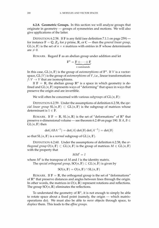
200 6. MODULES AND VECTOR SPACES
6.2.8. Geometric Groups. In this section we will analyze groups thatoriginate in geometry — groups of symmetries and motions. We will alsogive applications of the latter.
DEFINITION 6.2.58. If F is any field (see definition 7.1.1 on page 259) —for instance F = Q, Zp for p prime, R, or C — then the general linear group,GL(n, F) is the set of n× n matrices with entries in F whose determinantsare 6= 0.
REMARK. Regard F as an abelian group under addition and let
Fn = F⊕ · · · ⊕F︸ ︷︷ ︸n summands
In this case, GL(n, F) is the group of automorphisms of Fn. If V is a vector-space, GL(V) is the group of automorphisms of V, i.e., linear transformationsf : V → V that are isomorphisms.
If F = R, the abelian group Rn is a space in which geometry is de-fined and GL(n, F) represents ways of “deforming” that space in ways thatpreserve the origin and are invertible.
We will often be concerned with various subgroups of GL(n, F):
DEFINITION 6.2.59. Under the assumptions of definition 6.2.58, the spe-cial linear group SL(n, F) ⊂ GL(n, F) is the subgroup of matrices whosedeterminant is 1 ∈ F.
REMARK. If F = R, SL(n, R) is the set of “deformations” of Rn thatpreserve n-dimensional volume — see theorem 6.2.49 on page 190. If A, B ∈GL(n, F) then
det(ABA−1) = det(A)det(B)det(A−1) = det(B)
so that SL(n, F) is a normal subgroup of GL(n, F).
DEFINITION 6.2.60. Under the assumptions of definition 6.2.58, the or-thogonal group O(n, F) ⊂ GL(n, F) is the group of matrices M ∈ GL(n, F)with the property that
MMt = I
where Mt is the transpose of M and I is the identity matrix.The special orthogonal group, SO(n, F) ⊂ GL(n, F) is given by
SO(n, F) = O(n, F) ∩ SL(n, F)
REMARK. If F = R, the orthogonal group is the set of “deformations”of Rn that preserve distances and angles between lines through the origin.In other words, the matrices in O(n, R) represent rotations and reflections.The group SO(n, R) eliminates the reflections.
To understand the geometry of Rn, it is not enough to simply be ableto rotate space about a fixed point (namely, the origin — which matrix-operations do). We must also be able to move objects through space, todisplace them. This leads to the affine groups.
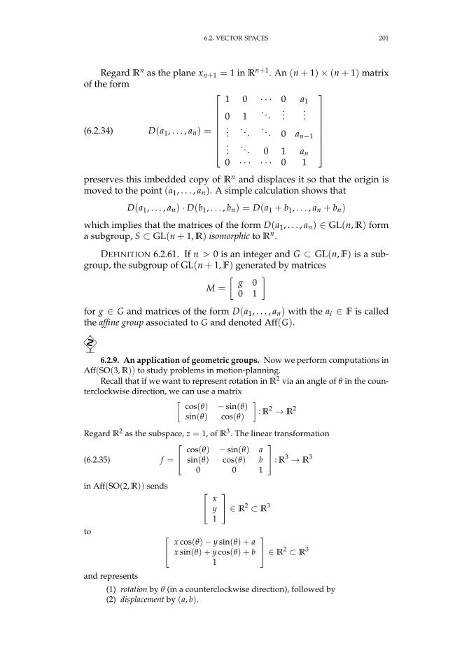
6.2. VECTOR SPACES 201
Regard Rn as the plane xn+1 = 1 in Rn+1. An (n + 1)× (n + 1) matrixof the form
(6.2.34) D(a1, . . . , an) =
1 0 · · · 0 a1
0 1. . .
......
.... . . . . . 0 an−1
.... . . 0 1 an
0 · · · · · · 0 1
preserves this imbedded copy of Rn and displaces it so that the origin ismoved to the point (a1, . . . , an). A simple calculation shows that
D(a1, . . . , an) · D(b1, . . . , bn) = D(a1 + b1, . . . , an + bn)
which implies that the matrices of the form D(a1, . . . , an) ∈ GL(n, R) forma subgroup, S ⊂ GL(n + 1, R) isomorphic to Rn.
DEFINITION 6.2.61. If n > 0 is an integer and G ⊂ GL(n, F) is a sub-group, the subgroup of GL(n + 1, F) generated by matrices
M =
[g 00 1
]for g ∈ G and matrices of the form D(a1, . . . , an) with the ai ∈ F is calledthe affine group associated to G and denoted Aff(G).
6.2.9. An application of geometric groups. Now we perform computations inAff(SO(3, R)) to study problems in motion-planning.
Recall that if we want to represent rotation in R2 via an angle of θ in the coun-terclockwise direction, we can use a matrix[
cos(θ) − sin(θ)sin(θ) cos(θ)
]: R2 → R2
Regard R2 as the subspace, z = 1, of R3. The linear transformation
(6.2.35) f =
cos(θ) − sin(θ) asin(θ) cos(θ) b
0 0 1
: R3 → R3
in Aff(SO(2, R)) sends xy1
∈ R2 ⊂ R3
to x cos(θ)− y sin(θ) + ax sin(θ) + y cos(θ) + b
1
∈ R2 ⊂ R3
and represents
(1) rotation by θ (in a counterclockwise direction), followed by(2) displacement by (a, b).
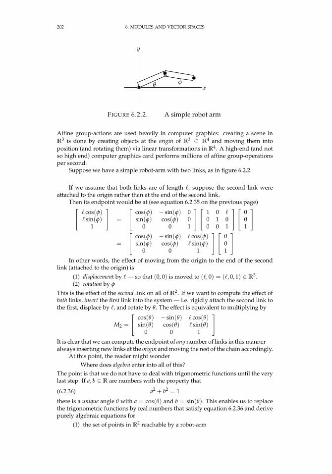
202 6. MODULES AND VECTOR SPACES
FIGURE 6.2.2. A simple robot arm
Affine group-actions are used heavily in computer graphics: creating a scene inR3 is done by creating objects at the origin of R3 ⊂ R4 and moving them intoposition (and rotating them) via linear transformations in R4. A high-end (and notso high end) computer graphics card performs millions of affine group-operationsper second.
Suppose we have a simple robot-arm with two links, as in figure 6.2.2.
If we assume that both links are of length `, suppose the second link wereattached to the origin rather than at the end of the second link.
Then its endpoint would be at (see equation 6.2.35 on the previous page) ` cos(φ)` sin(φ)
1
=
cos(φ) − sin(φ) 0sin(φ) cos(φ) 0
0 0 1
1 0 `0 1 00 0 1
001
=
cos(φ) − sin(φ) ` cos(φ)sin(φ) cos(φ) ` sin(φ)
0 0 1
001
In other words, the effect of moving from the origin to the end of the second
link (attached to the origin) is
(1) displacement by ` — so that (0, 0) is moved to (`, 0) = (`, 0, 1) ∈ R3.(2) rotation by φ
This is the effect of the second link on all of R2. If we want to compute the effect ofboth links, insert the first link into the system — i.e. rigidly attach the second link tothe first, displace by `, and rotate by θ. The effect is equivalent to multiplying by
M2 =
cos(θ) − sin(θ) ` cos(θ)sin(θ) cos(θ) ` sin(θ)
0 0 1
It is clear that we can compute the endpoint of any number of links in this manner —always inserting new links at the origin and moving the rest of the chain accordingly.
At this point, the reader might wonderWhere does algebra enter into all of this?
The point is that we do not have to deal with trigonometric functions until the verylast step. If a, b ∈ R are numbers with the property that
(6.2.36) a2 + b2 = 1
there is a unique angle θ with a = cos(θ) and b = sin(θ). This enables us to replacethe trigonometric functions by real numbers that satisfy equation 6.2.36 and derivepurely algebraic equations for
(1) the set of points in R2 reachable by a robot-arm
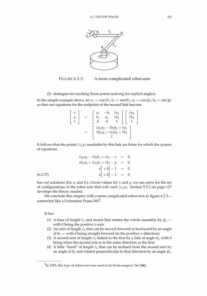
6.2. VECTOR SPACES 203
FIGURE 6.2.3. A more complicated robot arm
(2) strategies for reaching those points (solving for explicit angles).
In the simple example above, let a1 = cos(θ), b1 = sin(θ), a2 = cos(φ), b2 = sin(φ)so that our equations for the endpoint of the second link become x
y1
=
a1 −b1 `a1b1 a1 `b10 0 1
`a2`b21
=
`a1a2 − `b2b1 + `a1`b1a2 + `a1b2 + `b1
1
It follows that the points (x, y) reachable by this link are those for which the systemof equations
`a1a2 − `b2b1 + `a1 − x = 0`b1a2 + `a1b2 + `b1 − y = 0
a21 + b2
1 − 1 = 0
a22 + b2
2 − 1 = 0(6.2.37)
has real solutions (for ai and bi). Given values for x and y, we can solve for the setof configurations of the robot arm that will reach (x, y). Section 5.5.2 on page 127develops the theory needed.
We conclude this chapter with a more complicated robot-arm in figure 6.2.3—somewhat like a Unimation Puma 5605.
It has:
(1) A base of height `1 and motor that rotates the whole assembly by φ1 —with 0 being the positive x-axis.
(2) An arm of length `2 that can be moved forward or backward by an angleof θ1 — with 0 being straight forward (in the positive x-direction).
(3) A second arm of length `3 linked to the first by a link of angle θ2, with 0being when the second arm is in the same direction as the first.
(4) A little “hand” of length `4 that can be inclined from the second arm byan angle of θ3 and rotated perpendicular to that direction by an angle φ2.
5In 1985, this type of robot-arm was used to do brain-surgery! See [66].
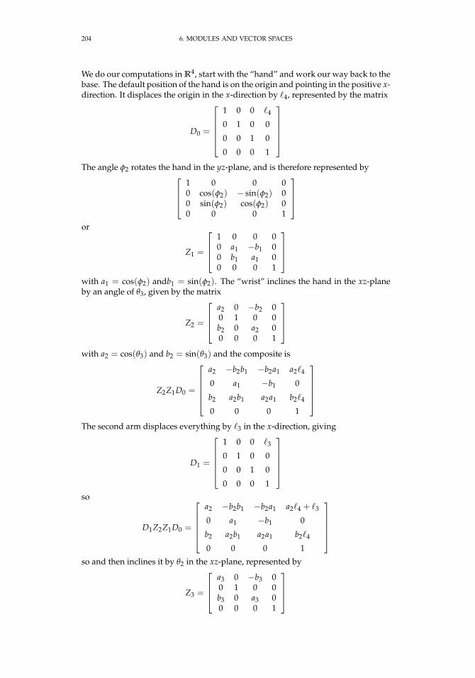
204 6. MODULES AND VECTOR SPACES
We do our computations in R4, start with the “hand” and work our way back to thebase. The default position of the hand is on the origin and pointing in the positive x-direction. It displaces the origin in the x-direction by `4, represented by the matrix
D0 =
1 0 0 `4
0 1 0 0
0 0 1 0
0 0 0 1
The angle φ2 rotates the hand in the yz-plane, and is therefore represented by
1 0 0 00 cos(φ2) − sin(φ2) 00 sin(φ2) cos(φ2) 00 0 0 1
or
Z1 =
1 0 0 00 a1 −b1 00 b1 a1 00 0 0 1
with a1 = cos(φ2) andb1 = sin(φ2). The “wrist” inclines the hand in the xz-planeby an angle of θ3, given by the matrix
Z2 =
a2 0 −b2 00 1 0 0b2 0 a2 00 0 0 1
with a2 = cos(θ3) and b2 = sin(θ3) and the composite is
Z2Z1D0 =
a2 −b2b1 −b2a1 a2`4
0 a1 −b1 0
b2 a2b1 a2a1 b2`4
0 0 0 1
The second arm displaces everything by `3 in the x-direction, giving
D1 =
1 0 0 `3
0 1 0 0
0 0 1 0
0 0 0 1
so
D1Z2Z1D0 =
a2 −b2b1 −b2a1 a2`4 + `3
0 a1 −b1 0
b2 a2b1 a2a1 b2`4
0 0 0 1
so and then inclines it by θ2 in the xz-plane, represented by
Z3 =
a3 0 −b3 00 1 0 0b3 0 a3 00 0 0 1
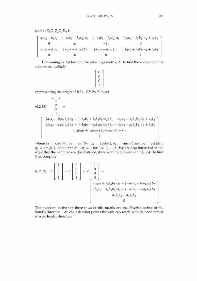
6.2. VECTOR SPACES 205
so that Z3D1Z2Z1D0 isa3a2 − b3b2 (−a3b2 − b3a2) b1 (−a3b2 − b3a2) a1 (a3a2 − b3b2) `4 + a3`3
0 a1 −b1 0
b3a2 + a3b2 (a3a2 − b3b2) b1 (a3a2 − b3b2) a1 (b3a2 + a3b2) `4 + b3`3
0 0 0 1
Continuing in this fashion, we get a huge matrix, Z. To find the endpoint of the
robot-arm, multiply 0001
(representing the origin of R3 ⊂ R4) by Z to get
(6.2.38)
xyz1
=
((a5a3 + b5b4b3) a2 + (−a5b3 + b5b4a3) b2) `4 + (a5a3 + b5b4b3) `3 + a5`2
((b5a3 − a5b4b3) a2 + (−b5b3 − a5b4a3) b2) `4 + (b5a3 − a5b4b3) `3 + b5`2
(a4b3a2 + a4a3b2) `4 + a4b3`3 + ` 1
1
where a3 = cos(θ2), b3 = sin(θ2), a4 = cos(θ1), b4 = sin(θ1) and a5 = cos(φ1),b5 = sin(φ1). Note that a2
i + b2i = 1 for i = 1, . . . , 5. We are also interested in the
angle that the hand makes (for instance, if we want to pick something up). To findthis, compute
(6.2.39) Z
1001
− Z
0001
= Z
1000
=
(a5a3 + b5b4b3) a2 + (−a5b3 + b5b4a3) b2
(b5a3 − a5b4b3) a2 + (−b5b3 − a5b4a3) b2
a4b3a2 + a4a3b2
0
The numbers in the top three rows of this matrix are the direction-cosines of thehand’s direction. We can ask what points the arm can reach with its hand aimedin a particular direction.
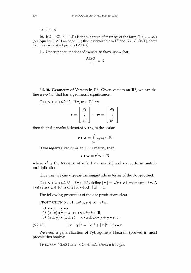
206 6. MODULES AND VECTOR SPACES
EXERCISES.
20. If S ⊂ GL(n + 1, F) is the subgroup of matrices of the form D(a1, . . . , an)(see equation 6.2.34 on page 201) that is isomorphic to Fn and G ⊂ GL(n, F), showthat S is a normal subgroup of Aff(G).
21. Under the assumptions of exercise 20 above, show that
Aff(G)
S∼= G
6.2.10. Geometry of Vectors in Rn. Given vectors on Rn, we can de-fine a product that has a geometric significance.
DEFINITION 6.2.62. If v, w ∈ Rn are
v =
v1...
vn
, w =
w1...
wn
then their dot-product, denoted v •w, is the scalar
v •w =n
∑i=1
viwi ∈ R
If we regard a vector as an n× 1 matrix, then
v •w = vtw ∈ R
where vt is the transpose of v (a 1 × n matrix) and we perform matrix-multiplication.
Give this, we can express the magnitude in terms of the dot-product:
DEFINITION 6.2.63. If v ∈ Rn, define ‖v‖ = √v • v is the norm of v. Aunit vector u ∈ Rn is one for which ‖u‖ = 1.
The following properties of the dot-product are clear:
PROPOSITION 6.2.64. Let x, y ∈ Rn. Then:
(1) x • y = y • x(2) (k · x) • y = k · (x • y), for k ∈ R,(3) (x± y) • (x± y) = x • x± 2x • y + y • y, or
(6.2.40) ‖x± y‖2 = ‖x‖2 + ‖y‖2 ± 2x • y
We need a generalization of Pythagoras’s Theorem (proved in mostprecalculus books):
THEOREM 6.2.65 (Law of Cosines). Given a triangle:
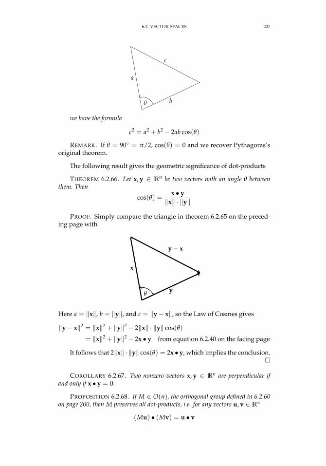
6.2. VECTOR SPACES 207
b
c
a
θ
we have the formula
c2 = a2 + b2 − 2ab cos(θ)
REMARK. If θ = 90 = π/2, cos(θ) = 0 and we recover Pythagoras’soriginal theorem.
The following result gives the geometric significance of dot-products
THEOREM 6.2.66. Let x, y ∈ Rn be two vectors with an angle θ betweenthem. Then
cos(θ) =x • y‖x‖ · ‖y‖
PROOF. Simply compare the triangle in theorem 6.2.65 on the preced-ing page with
y
y− x
x
θ
Here a = ‖x‖, b = ‖y‖, and c = ‖y− x‖, so the Law of Cosines gives
‖y− x‖2 = ‖x‖2 + ‖y‖2 − 2‖x‖ · ‖y‖ cos(θ)
= ‖x‖2 + ‖y‖2 − 2x • y from equation 6.2.40 on the facing page
It follows that 2‖x‖ · ‖y‖ cos(θ) = 2x • y, which implies the conclusion.
COROLLARY 6.2.67. Two nonzero vectors x, y ∈ Rn are perpendicular ifand only if x • y = 0.
PROPOSITION 6.2.68. If M ∈ O(n), the orthogonal group defined in 6.2.60on page 200, then M preserves all dot-products, i.e. for any vectors u, v ∈ Rn
(Mu) • (Mv) = u • v
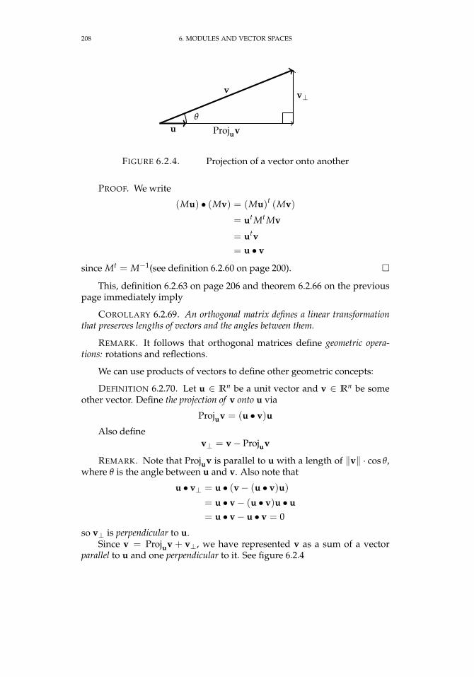
208 6. MODULES AND VECTOR SPACES
u
v
Projuv
v⊥
θ
FIGURE 6.2.4. Projection of a vector onto another
PROOF. We write
(Mu) • (Mv) = (Mu)t (Mv)
= ut Mt Mv
= utv= u • v
since Mt = M−1(see definition 6.2.60 on page 200).
This, definition 6.2.63 on page 206 and theorem 6.2.66 on the previouspage immediately imply
COROLLARY 6.2.69. An orthogonal matrix defines a linear transformationthat preserves lengths of vectors and the angles between them.
REMARK. It follows that orthogonal matrices define geometric opera-tions: rotations and reflections.
We can use products of vectors to define other geometric concepts:
DEFINITION 6.2.70. Let u ∈ Rn be a unit vector and v ∈ Rn be someother vector. Define the projection of v onto u via
Projuv = (u • v)u
Also definev⊥ = v− Projuv
REMARK. Note that Projuv is parallel to u with a length of ‖v‖ · cos θ,where θ is the angle between u and v. Also note that
u • v⊥ = u • (v− (u • v)u)
= u • v− (u • v)u • u= u • v− u • v = 0
so v⊥ is perpendicular to u.Since v = Projuv + v⊥, we have represented v as a sum of a vector
parallel to u and one perpendicular to it. See figure 6.2.4
6.2. VECTOR SPACES 209
EXERCISES.
22. Compute the angle between the vectors 123
and
1−20
23. If u1, . . . , un ∈ Rnare an orthonormal basis, show that the matrix
M =
u1...
un
— i.e. the matrix whose rows are the ui, is an orthogonal matrix — i.e.defines an element of O(n) in definition 6.2.60 on page 200.
24. Suppose A is a symmetric matrix (i.e., A = At). If (λ1, v1) and(λ2, v2) are eigenvalue-eigenvector pairs with λ1 6= λ2, show that v1 • v2 =0. Hint: If a vector is regarded as an n× 1 matrix, its transpose is a 1× nmatrix and utv = u • v — i.e. the matrix product is the dot-product.
6.2.11. Vectors in R3. Besides the dot-product, there’s another way toform products of vectors — that is only well-defined in R3 (to see what hap-pens in other dimensions, look at the discussion following corollary 10.7.13on page 379).
DEFINITION 6.2.71. Define vectors
i =
100
, j =
010
, k =
001
so that vectors in R3 can be written as linear combinations of i, j, and k.Given this definition and vectors in R3
x =
x1x2x3
, y =
y1y2y3
set
(6.2.41) x× y = det
i j kx1 x2 x3y1 y2 y3
— the cross product of x and y.
REMARK. Expansions by minors in the first row (see definitions 6.2.37on page 182 and proposition 6.2.36 on page 182) gives
(6.2.42) x× y = i ·det[
x2 x3y2 y3
]− j ·det
[x1 x3y1 y3
]+ k ·det
[x1 x2y1 y2
]We have the following properties of cross-products:
210 6. MODULES AND VECTOR SPACES
PROPOSITION 6.2.72. Given vectors
x =
x1x2x3
, y =
y1y2y3
, z =
z1z2z3
then
(1) (x + y)× z = x× z + y× z(2) y× x = −x× y(3) x× x = 0(4)
x • (y× z) = det
x1 x2 x3y1 y2 y3z1 z2 z3
(5) so x • (x× y) = y • (x× y) = 0 so x× y is perpendicular to x and y.
PROOF. The first statement follows from corollary 6.2.27 on page 174,proposition 6.2.23 on page 173, and corollary 6.2.17 on page 171.
Statement 2 follows from proposition 6.2.20 on page 172, and state-ment 3 follows from equation 6.2.42 on the previous page, which impliesthat
x • (y× z) = x1 · det[
y2 y3z2 z3
]− x2 · det
[y1 y3z1 z3
]+ x3 · det
[y1 y2z1 z2
]
= det
x1 x2 x3y1 y2 y3z1 z2 z3
by proposition 6.2.37 on page 182.
Statement 4 and theorem 6.2.49 on page 190 implies that:
COROLLARY 6.2.73. Given vectors
x =
x1x2x3
, y =
y1y2y3
, z =
z1z2z3
the composite
x • (y× z)is equal to the volume of the parallelepiped spanned by x, y, and z.
This leads to a geometric interpretation of x× y:
PROPOSITION 6.2.74. If x and y are vectors in R3 with an angle of θ betweenthem, then
‖x× y‖ = ‖x‖ · ‖y‖ · sin(θ)— the area of the parallelogram generated by x and y.
REMARK. This almost completes a geometric description of x × y: itis perpendicular to x and y and has the length given above. The vectorhas two possible directions and the one it takes is given by the Right HandRule: if fingers of the right hand go from x and y, the thumb points in thedirection of x× y.
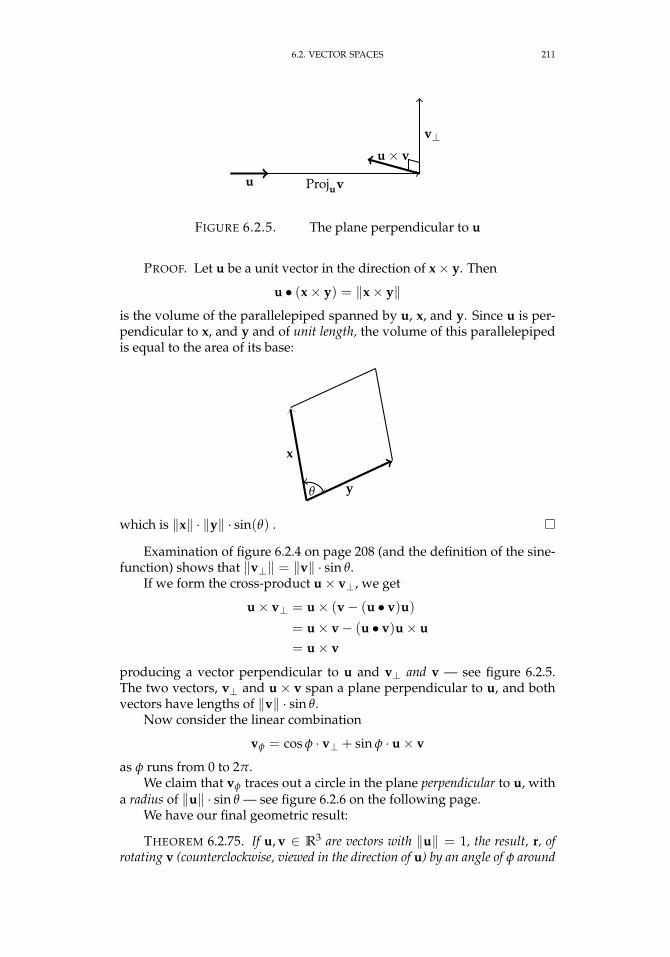
6.2. VECTOR SPACES 211
u Projuv
v⊥u× v
FIGURE 6.2.5. The plane perpendicular to u
PROOF. Let u be a unit vector in the direction of x× y. Then
u • (x× y) = ‖x× y‖is the volume of the parallelepiped spanned by u, x, and y. Since u is per-pendicular to x, and y and of unit length, the volume of this parallelepipedis equal to the area of its base:
y
x
θ
which is ‖x‖ · ‖y‖ · sin(θ) .
Examination of figure 6.2.4 on page 208 (and the definition of the sine-function) shows that ‖v⊥‖ = ‖v‖ · sin θ.
If we form the cross-product u× v⊥, we get
u× v⊥ = u× (v− (u • v)u)
= u× v− (u • v)u× u= u× v
producing a vector perpendicular to u and v⊥ and v — see figure 6.2.5.The two vectors, v⊥ and u× v span a plane perpendicular to u, and bothvectors have lengths of ‖v‖ · sin θ.
Now consider the linear combination
vφ = cos φ · v⊥ + sin φ · u× v
as φ runs from 0 to 2π.We claim that vφ traces out a circle in the plane perpendicular to u, with
a radius of ‖u‖ · sin θ — see figure 6.2.6 on the following page.We have our final geometric result:
THEOREM 6.2.75. If u, v ∈ R3 are vectors with ‖u‖ = 1, the result, r, ofrotating v (counterclockwise, viewed in the direction of u) by an angle of φ around
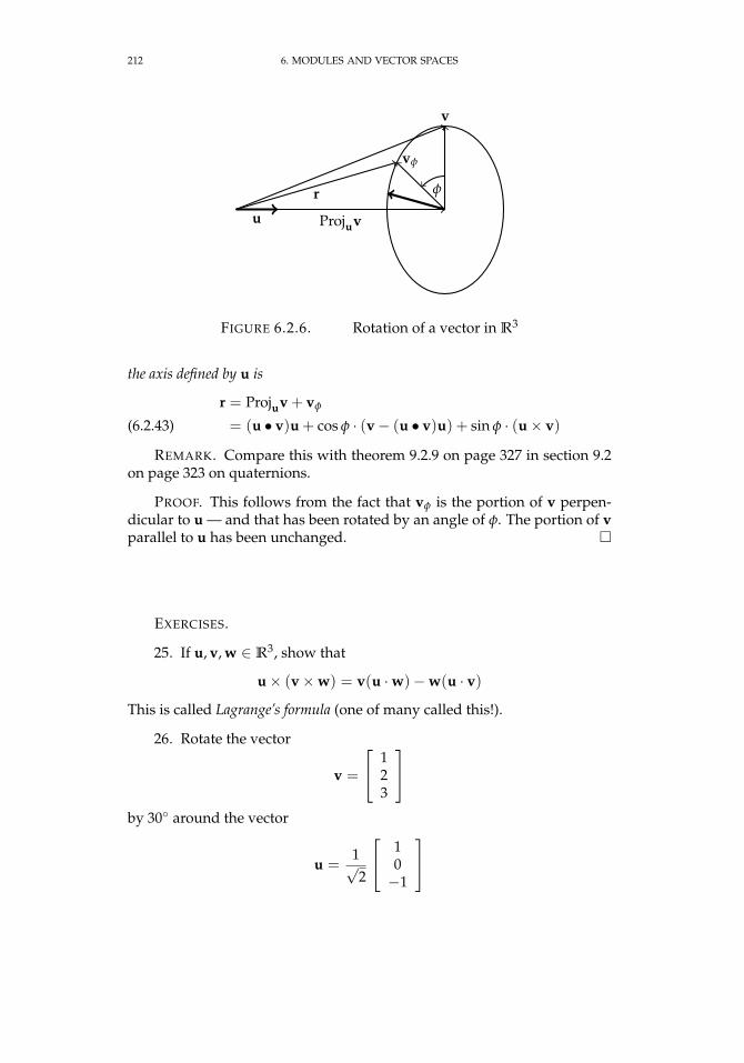
212 6. MODULES AND VECTOR SPACES
u
v
Projuv
vφ
r φ
FIGURE 6.2.6. Rotation of a vector in R3
the axis defined by u is
r = Projuv + vφ
= (u • v)u + cos φ · (v− (u • v)u) + sin φ · (u× v)(6.2.43)
REMARK. Compare this with theorem 9.2.9 on page 327 in section 9.2on page 323 on quaternions.
PROOF. This follows from the fact that vφ is the portion of v perpen-dicular to u — and that has been rotated by an angle of φ. The portion of vparallel to u has been unchanged.
EXERCISES.
25. If u, v, w ∈ R3, show that
u× (v×w) = v(u ·w)−w(u · v)This is called Lagrange’s formula (one of many called this!).
26. Rotate the vector
v =
123
by 30 around the vector
u =1√2
10−1
6.2. VECTOR SPACES 213
6.2.12. Inner-product spaces over R and C. Inner product spaces arevector space equipped with an analogue to the dot product, called an innerproduct:
DEFINITION 6.2.76. A vector space, V, over k = R or C is called aHilbert space if it has a function
〈∗, ∗〉 : V ×V → k
called its inner product, such that(1) 〈α · v1 + β · v2, w〉 = α · 〈v1, w〉+ β · 〈v2, w〉 for all α, β ∈ k , and
v1, v2, w ∈ V,(2) 〈v, w〉 = 〈w, v〉, the complex conjugate, for all v, w ∈ V. Note
that this implies 〈v, v〉 = 〈v, v〉, or that 〈v, v〉 ∈ R for all v ∈ V.(3) 〈v, v〉 = 0 implies that v = 0.(4) Define ‖v‖ =
√〈v, v〉
(5) Let vi be an infinite sequence of elements of V. If the series∞
∑n=1‖vi‖
converges, then so does∞
∑n=1
vi
REMARK. The first rule implies that 〈0, v〉 = 〈v, 0〉 = 0.We have already seen an example of an inner product space over R,
namely Rn, equipped with the dot product — see 6.2.62 on page 206.It turns out that the last condition is always satisfied if V is finite-
dimensional (the proof is beyond the scope of this book!). We mention ithere because many interesting Hilbert spaces are infinite-dimensional.
We have a version of the last statement in proposition 6.2.64 onpage 206
PROPOSITION 6.2.77. If V is an inner product space and x, y ∈ V, then
‖x± y‖2 = ‖x‖2 + ‖y‖2 ± 〈x, y〉 ± 〈y, x〉In particular, if 〈x, y〉 = 0 then
‖x± y‖2 = ‖x‖2 + ‖y‖2
PROOF. Straightforward computation:
〈x± y, x± y〉 = 〈x, x〉 ± 〈x, y〉± 〈y, x〉+ (±1)2 〈y, y〉
DEFINITION 6.2.78. Let V = Cn for some finite n > 0. For any v, w ∈ Vdefine the standard inner product via
〈v, w〉 =n
∑i=1
viwi
214 6. MODULES AND VECTOR SPACES
Even over the real numbers, we can have spaces with “exotic” innerproducts:
EXAMPLE 6.2.79. Let
M =
2 −1 0−1 2 −10 −1 2
and define an inner product in R3 via
〈v, w〉 = vt Mw
This is clearly bilinear (i.e., it satisfies rules 1 and 2). We must verify rule 3:If
v =
xyz
then
〈v, v〉 = vt Mv =[
x y z] 2 −1 0−1 2 −10 −1 2
xyz
=[
2x− y, −x + 2y− z, −y + 2z] x
yz
= 2x2 − 2xy + 2y2 − 2yz + 2z2
= x2 + (x− y)2 + (y− z)2 + z2
≥ 0
If 〈v, v〉 = 0, it follows that x = 0 = z and x = y so v = 0.If
e1 =
100
, e2 =
010
, e3 =
001
is the standard basis for R3, 〈e1, e1〉 = 2 so the norm of e1with this newinner-product is √
〈e1, e1〉 =√
2
Since 〈e1, e2〉 = −1, e1 and e2 are not even perpendicular in this newinner-product.
Here’s an example of an infinite dimensional Hilbert space used heav-ily in functional analysis:
EXAMPLE 6.2.80. If a, b ∈ R with a < b define L2([a, b]) to be the set ofequivalence classes of complex-valued functions, f , on [a, b] with∫ b
a‖ f (x)‖2dx < ∞
where two functions f , g are regarded as equivalent if∫ b
a‖ f (x)− g(x)‖2dx = 0
6.2. VECTOR SPACES 215
and with an inner product defined by
〈 f , g〉 =∫ b
af (x)g(x)dx
From now on, we’ll only be concerned with finite-dimensional Hilbertspaces like example 6.2.78 on page 213.
DEFINITION 6.2.81. Given an n × n matrix, A, with complex entries,define the Hermitian transpose, AH , via(
AH)
i,j= Aj,i
A matrix, A, is called Hermitian if
A = AH
A n× n matrix, U, is called unitary if
UUH = UHU = I
REMARK. Note that these are direct generalizations of familiar con-cepts to the complex domain: a real-valued Hermitian matrix is symmetric,and a real-valued unitary matrix is orthogonal.
Charles Hermite (1822 – 1901) was a French mathematician who did re-search involving number theory, quadratic forms, invariant theory, orthog-onal polynomials, elliptic functions, and algebra. He was the first to provethat e is a transcendental number.The Hermite crater near the Moon’s north pole is named in his honor.
Proof of the following two statements is left as an exercise for thereader:
PROPOSITION 6.2.82. The product of two unitary matrices is unitary, so theset of n× n unitary matrices form a group, U(n). If A and B are complex-valuedmatrices then
(AB)H = BH AH
REMARK. Note that the standard inner product on Cn can be definedas the matrix-product
〈u, v〉 = uHv
We have a unitary version of proposition 6.2.68 on page 207:
PROPOSITION 6.2.83. Let V = Cn with the standard inner product (seedefinition 6.2.78 on page 213) and let U be a unitary matrix. If v, w ∈ V then
〈Uv, Uw〉 = 〈v, w〉PROOF. Straight computation:
〈Uv, Uw〉 = (Uv)HUw
= vHUHUw
= vHw
= 〈v, w〉
216 6. MODULES AND VECTOR SPACES
We start with:
DEFINITION 6.2.84. Let V be an inner product space and letu1, . . . , uk ∈ V be a set of vectors. This set is defined to be orthonormal if
(6.2.44)⟨ui, uj
⟩=
1 if i = j0 otherwise
Unitary matrices are a complex analogue to orthogonal matrices (seeexercise 23 on page 209):
PROPOSITION 6.2.85. If
M =[
v1 · · · vn]
be an n× n matrix with entries in C and column-vectors v1, · · · , vn , then M isunitary if and only if the vi form an orthonormal set with respect to the standardinner product (see definition 6.2.78 on page 213).
PROOF. We haveMH M = A
whereAi,j = vH
i vj =⟨vi, vj
⟩
As with vector spaces over R, we can define projections:
DEFINITION 6.2.86. If V is an inner-product space, v ∈ V, and S =u1, . . . , uk is an orthonormal set of vectors with W = Span(S) (see defi-nition 6.2.3 on page 164), then define
ProjWv =k
∑i=1〈ui, v〉 ui
REMARK. If V is over the complex numbers, we’ve lost the precise geo-metric significance of projection.
It is easy to express vectors in terms of an orthonormal basis
PROPOSITION 6.2.87. Let V be an inner product space over k (R or C) withan orthonormal basis u1, . . . , un and let v ∈ V be any vector. Then
v =n
∑i=1〈v, ui〉 u = ProjVv
PROOF. Since u1, . . . , un is a basis for V, there is a unique expression
v =n
∑i=1
aiui
with ai ∈ k. If we take the inner product⟨v, uj
⟩=
n
∑i=1
ai⟨ui, uj
⟩= aj
due to equation 6.2.44.
6.2. VECTOR SPACES 217
Consider an inner product space, V. If S = u1, . . . , uk is an or-thonormal set of vectors that don’t span V, they span some vector subspaceW ⊂ V. Proposition 6.2.87 on the facing page tells us that if v ∈W
v = ProjWv
This raises the question:
If v /∈W, what is the relation between v and ProjWv?
PROPOSITION 6.2.88. If V is an inner product space, S = u1, . . . , uk isan orthonormal set of vectors that span W ⊂ V, and v is any other vector, then
v⊥ = v− ProjWv
has the property that⟨v⊥, uj
⟩= 0 for all j = 1, . . . , k, making it perpendicular to
all of W. It follows that ProjWv is the vector in W closest to v in the sense that
‖v−w‖ > ‖v− ProjWv‖for any w ∈W with w 6= ProjWv.
REMARK. This result shows the advantages of having orthonormalbases for vector spaces — in this case, W.
PROOF. If we form the inner product⟨v⊥, uj
⟩for any j = 1, . . . , k, we
get
⟨v− ProjWv, uj
⟩=⟨v, uj
⟩−⟨
k
∑i=1〈v, ui〉 ui, uj
⟩
=⟨v, uj
⟩−
k
∑i=1
⟨〈v, ui〉 ui, uj
⟩=⟨v, uj
⟩−⟨v, uj
⟩ ⟨uj, uj
⟩by equation 6.2.44
= 0
It follows that, if w ∈W, then 〈v⊥, w〉 = 0.Suppose v′ ∈W is a vector. Note that
v− v′ = (v− ProjWv) + (ProjWv− v′)
= v⊥ + (ProjWv− v′)
Since w = ProjWv− v′ ∈W, we have
〈v⊥, w〉 = 0
Proposition 6.2.77 on page 213 implies that
‖v− v′‖2 = ‖v⊥‖2 + ‖w‖2
so that ‖v− v′‖ > ‖v− ProjWv‖ = ‖v⊥‖ for all v′ 6= ProjWv.
Given the power of an orthonormal basis, it is gratifying that we canalways find one:
218 6. MODULES AND VECTOR SPACES
THEOREM 6.2.89 (Gram-Schmidt orthonormalization). Let v1, . . . , vk ∈V be a basis for an inner-product space, V over k = R or C. Then there exists anorthonormal basis
u1, . . . , uk
for V such that
(6.2.45) Span(u1, . . . , ui) = Span(v1, . . . , vi)
for i = 1, . . . , k.
REMARK. This is named after Jørgen Pedersen Gram and ErhardSchmidt but it appeared earlier in the work of Laplace and Cauchy6.
PROOF. This is an inductive process: We initially set
u1 =v1
‖v1‖Having performed j− 1 steps, define Wj = Span(u1, . . . , uj−1) ⊂ V and set
uj =vj − ProjWj
vj
‖vj − ProjWjvj‖
and continue until j = k. The process works because vj−ProjWjvj 6= 0 since:
(1) the u1, . . . , uj−1 are linear combinations of the v1, . . . , vj−1 — in away that is easily reversed7 — so the span of u1, . . . , uj−1 is the sameas that of v1, . . . , vj−1 — i.e., equation 6.2.45.
(2) the v1, . . . , vk are linearly independent, so vj is not in the span ofv1, . . . , vj−1 — or that of u1, . . . , uj−1 .
PROPOSITION 6.2.90. The eigenvalues of a Hermitian matrix lie in R.
PROOF. Let A be an n × n Hermitian matrix witheigenvalue-eigenvector pair (λ, v). Then
(6.2.46) Av = λv
If we form the Hermitian transpose, we get
(6.2.47) vH AH = λvH
Now, we left-multiply equation 6.2.46 by vH and right multiply equa-tion 6.2.47 by v, we get
vH Av = vHλv = λ‖v‖2
vH AHv = λ‖v‖2
Since A = AH , λ‖v‖2 = λ‖v‖2, and since ‖v‖2 6= 0, we conclude thatλ = λ or λ ∈ R.
Since real-valued matrices are Hermitian if and only if they are symmet-ric, we also conclude:
6Part of the mathematical tradition of naming things after people who didn’t discoverthem!
7So the vi can be written as linear combinations of the ui .
6.2. VECTOR SPACES 219
COROLLARY 6.2.91. The eigenvalues of a real-valued symmetric matrix liein R.
REMARK. It’s interesting that we must go into the complex domain toprove this statement about real matrices.
Although many matrices cannot be diagonalized (see example 6.2.56on page 197), there is an important class of them that can. We begin with:
LEMMA 6.2.92. If A is a complex-valued n× n matrix, then there exists ann× n unitary matrix, U, such that
U−1 AU = B
where B has the form
B =
[λ ∗0 A1
]where A1 is an (n− 1)× (n− 1) matrix and the first column of B has zeros belowthe first row. If A is real-valued, so are U and B.
PROOF. Let λ be an eigenvalue of A with eigenvector v. By adjoiningother vectors, we extend v to a basis for Cn and perform Gram-Schmidt or-thonormalization (theorem 6.2.89 on the facing page) to get an orthonormalbasis u1, . . . , un. We create a matrix with the ui as its columns:
U =[
u1 · · · un]
This will be unitary, by proposition 6.2.85 on page 216. In the new ui-basis,the linear transformation that A defines will have a matrix representationthat looks like B — since u1 = v/‖v‖ is still an eigenvector correspondingto the eigenvalue λ.
COROLLARY 6.2.93. If A is an n × n matrix over C, then there exists ann × n unitary matrix, U, such that U−1 AU is upper-triangular. If A is real-valued, so is U.
PROOF. Simply apply lemma 6.2.92 to A, and then to A1 and thesmaller matrices that result. After n− 1 such applications, we get
U−1n−1 · · ·U−1
1 AU1 · · ·Un−1
is upper-triangular, where U = U1 · · ·Un−1.
THEOREM 6.2.94. If A is a Hermitian n × n matrix, then there exists ann× n unitary matrix, U, such that U−1 AU is diagonal. If A is real-valued, so isU.
PROOF. Let U be such that B = U−1 AU is upper-triangular. We claimthat B is also Hermitian. Note that U−1 = UHand take the Hermitian trans-pose of
B = UH AUWe get
BH = UH AHU = UH AU = BBut a Hermitian upper-triangular matrix is diagonal.
220 6. MODULES AND VECTOR SPACES
Since a real-valued matrix is Hermitian if and only if it is symmetric,and unitary if and only if it is orthogonal, we get:
COROLLARY 6.2.95. If A is an n × n real-valued symmetric matrix, thenthere exists an n× n orthogonal matrix, U, such that U−1 AU is diagonal.
REMARK. This is interesting because it says not only that a symmetricmatrix can be diagonalized, but that this can be done by geometric operations:rotations and/or reflections.
Here’s an intuitive argument for why symmetric matrices can be diag-onalized: Every matrix is arbitrarily “close” to one with distinct eigenval-ues. For instance, we can we can perturb the matrix in example 6.2.56 onpage 197 so it has two distinct eigenvalues:[
1− ε 10 1 + ε
]namely 1− ε and 1 + ε. The eigenvectors corresponding to these are, re-spectively [
10
]and
[12ε
]As we let ε approach 0 the eigenvalues and eigenvectors merge, and theeigenvectors no longer span R2.
Exercise 24 on page 209 shows that the eigenvectors of a symmetricmatrix are orthogonal — so they cannot merge, even if the eigenvalues do —i.e., the angle between two vectors is a continuous function of the vectors,so it cannot abruptly jump from 90 to 0.
EXERCISES.
27. Find an orthonormal basis for R3, using the inner-product in ex-ample 6.2.79 on page 214 (use the Gram-Schmidt process).
6.3. Modules
6.3.1. Basic properties. Modules are like vector-spaces over ringsrather than fields. This turns out to make the subject infinitely morecomplex and many basic questions have no known general answers.
DEFINITION 6.3.1. If R is a commutative ring, a module over R is(1) an abelian group, A,(2) an action of R on A, i.e. a map
f : R× A→ A
such thatf (r, ∗): r× A→ A
6.3. MODULES 221
is a homomorphism of abelian groups, for all r ∈ R, and
f (r1, f (r2, a)) = f (r1r2, a)
andf (r1 + r2, a) = f (r1, a) + f (r2, a)
This action is usually written with a product-notation, i.e. f (r, a) = r · a (inanalogy with multiplication by scalars in a vector space).
If B ⊂ A is a subgroup with the property that r · B ⊂ B for all r ∈ R,then B is called a submodule of A. If R is not commutative, we can haveleft- or right-modules over R, and they are generally not equivalent to eachother. This definition given here is for a left module.
EXAMPLE. We can regard a ring, R, as a module over itself. Its submod-ules are precisely its ideals.
If g: R→ S is a homomorphism of rings, S naturally becomes a moduleover R by defining r · s = g(r)s for all r ∈ R and s ∈ S.
EXAMPLE 6.3.2. If R is a ring and Rn =⊕n
i=1 R, then Rn is a moduleover R with the action defined by multiplication in R. This is called the freemodule of rank n over R. An n-dimensional vector space over a field k is a freemodule of rank n over that field.
It is possible to come up with more “exotic” examples of modules:
EXAMPLE 6.3.3. Let V be an n-dimensional vector space over a field Fand let M be an n× n matrix over F. Then V is a module over the polyno-mial ring k[X], where a polynomial, p(X) ∈ k[X] acts via
p(M): V → V
In other words, we plug M into p(X) to get a matrix and then act on V viathat matrix.
Note that a vector-subspace W ⊂ V is a submodule if and only ifM(W) ⊂ W. It follows that the module-structure of V over k[X] dependsstrongly on the matrix M.
DEFINITION 6.3.4. Let M1 and M2 be modules over the same ring, R.A homomorphism of modules is a map of their underlying abelian groups
f : M1 → M2
such that f (r ·m) = r · f (m) for all m ∈ M and r ∈ R. The set of elementsm ∈ M1 with f (m) = 0 is called the kernel of f and denoted ker f . The set ofelements m ∈ M2 of the form f (n) for some n ∈ M1 is called the image of fand denoted im f .
If ker f = 0, the homomorphism f is said to be injective. If im f =M2, the homomorphism is said to be surjective. If f is both injective andsurjective, it is called an isomorphism.
REMARK. Note that, if f above is injective, we can regard M1 as a sub-module of M2. Isomorphic modules are algebraically equivalent.
The corresponding statements about abelian groups imply that

222 6. MODULES AND VECTOR SPACES
PROPOSITION 6.3.5. Let M be a module over a ring R and let A and B besubmodules of M. Then:
(1) we can define the quotient M/A as the set of equivalence classes of theequivalence relation
m1 ≡ m2 (mod A)
if m1 − m2 ∈ A, for all m1, m2 ∈ M. We can also define M/A as theset of cosets m + A for m ∈ M.
(2) the mapp: M→ M/A
sending an element to its equivalence class, is a homomorphism of mod-ules.
(3) the map p defines a 1-1 correspondence between submodules of M con-taining A and submodules of M/A
(4) there is a canonical isomorphism
A + BA
∼= BA ∩ B
DEFINITION 6.3.6. If f : M1 → M2 is a homomorphism of modules, thequotient
M2
f (M1)
is called the cokernel of f .
REMARK. Since one can form quotients of modules with respect to ar-bitrary submodules, cokernels always exist for module-homomorphisms.
DEFINITION 6.3.7. A sequence of modules and homomorphisms (allover the same ring)
· · · fn+1−−→ Mn+1fn−→ Mn
fn−1−−→ Mn−1 → · · ·is said to be exact if im fn+1 = ker fn for all n. An exact sequence with fiveterms like
0→ Af−→ B
g−→ C → 0
is called a short exact sequence.
REMARK. In the short exact sequence above, the kernel of f must be0, so A can be identified with a submodule of B, and the map g must besurjective (since the kernel of the rightmost map is all of C).
The exactness of the (long) sequence above is equivalent to saying thatthe short sequences
0→ im fn → Mn → im fn−1 → 0
are exact for all n.Exact sequences are widely used in homological algebra and algebraic
topology, facilitating many types of computations.
6.3. MODULES 223
DEFINITION 6.3.8. If M is a module over a ring R, a set of elementsS = m1, . . . ∈ M will be called a generating set if every element m ∈ Mcan be expressed in terms of the elements of S
m = ∑mi∈S
ri ·mi
with the ri ∈ R.A module is said to be finitely generated if it has a finite generating set.
EXAMPLE 6.3.9. As in example 6.3.3 on page 221Let V be ann-dimensional vector space over a field F and let M be the n × npermutation matrix
M =
0 0 0 · · · 10 1 0 · · · 0
0 0 1. . . 0
1 0 0 · · · 0
Then, as a module over k[X] (defined as in example 6.3.3 on page 221), Vhas a single generator, namely
g =
10...0
This is because
Mg =
01...0
and Mkg = gk, the kth basis element of V. So all of the basis-elements of Vare in the orbit of powers of M and of k[X].
In analogy with proposition 4.6.7 on page 62, we have:
PROPOSITION 6.3.10. Every R-module is a quotient of a free R-module.
PROOF. If M is an R-module with generating set m1, . . . , let F be freeon generators e1, . . . — one for each of the mi. We define a map
f : F → M
∑ rjej 7→∑ rjmj
This is clearly surjective, so that
Fker f
∼= M
224 6. MODULES AND VECTOR SPACES
It is interesting to consider what properties of vector-spaces carry overto modules, or whether we can do a kind of “linear algebra” over a generalring. This is a deep field of mathematics that includes several areas, suchas group-representations (see [40]), homological algebra (see [109]) and al-gebraic K-theory (see [74]).
Even a simple question like“Is a submodule of a finitely generated module finitelygenerated?”
can have a complex answer. For instance, let R = k[X1, . . . ] — a polyno-mial ring over an infinite number of variables. It is finitely generated as amodule over itself (generated by 1). The submodule of polynomials withvanishing constant term is not finitely generated since every polynomialhas a finite number of variables.
We need to find a class of modules that is better-behaved.
DEFINITION 6.3.11. A module M over a ring R will be called noetherianif all of its submodules are finitely generated — this is equivalent to sayingthat all ascending chains of submodules of M
M1 ⊂ M2 ⊂ · · · ⊂ Mi ⊂ · · ·becomes constant from some finite point on, i.e. Mt = Mt+i for all i > 0. Amodule will be said to be Artinian if every descending chain of submodules
M1 ⊃ M2 ⊃ · · · ⊂ Mi ⊃ · · ·becomes constant from some finite point on.
REMARK. A ring is noetherian if and only if it is noetherian as a moduleover itself.
PROPOSITION 6.3.12. Let
0→ M1f−→ M2
g−→ M3 → 0
be a short exact sequence (see definition 6.3.7 on page 222) of modules over a ring.Then M2 is noetherian or Artinian if and only if M1 and M3 are both noetherianor Artinian, respectively.
PROOF. We will prove this in the noetherian case; the Artinian case isalmost identical. Clearly, if M2 is noetherian, M1 will inherit this propertysince it is a submodule. Any increasing chain of submodules of M3 will liftto one in M2, which becomes constant from some finite point on. It followsthat M2 being noetherian implies that M1 and M3 are also noetherian.
Conversely, suppose that M1 and M3 are noetherian and
N1 ⊂ N2 ⊂ · · · ⊂ Ni ⊂ · · ·is an increasing sequence of submodules of M2. Since M3 is noetherian, thisimage of this sequence in M3 will become constant from some finite pointon, say k. Then
(6.3.1)Ni
Ni ∩M1=
Ni+1
Ni+1 ∩M1
6.3. MODULES 225
for i > k. Since M1 is noetherian, the sequence
Nj ∩M1 ⊂ Nj+1 ∩M2 ⊂ · · ·will become constant from some finite point on — say j = t. Then, fori > max(k, t), equation 6.3.1 on the facing page and
Ni ∩M1 = Ni+1 ∩M1
imply that Ni = Ni+1.
COROLLARY 6.3.13. If R is a noetherian ring, then Rn is a noetherian mod-ule.
PROOF. This is a simple induction on n. If n = 1, R1 = R is noetherianover itself since it is a noetherian ring. For n > 1 we use proposition 6.3.12on the preceding page with the short exact sequence
0→ Rf−→ Rn+1 g−→ Rn → 0
where
g(r1, . . . , rn+1) = (r1, . . . , rn)
f (r) = (0, . . . 0, r)
where the image of f is the n + 1st entry in Rn+1.
Now we can define a large class of well-behaved modules:
LEMMA 6.3.14. If R is a noetherian ring, a module, M over R is noetherianif and only if it is finitely generated.
PROOF. If M is noetherian it must be finitely generated (since its sub-modules, including itself, are). Suppose M is finitely generated, say bygenerators (a1, . . . , an). Then there exists a surjective homomorphism ofmodules
Rn f−→ M(r1, . . . , rn) 7→ r1 · a1 + · · ·+ rn · an
This map fits into a short exact sequence
0→ ker f → Rn f−→ M→ 0
and proposition 6.3.12 on the facing page and corollary 6.3.13 imply theconclusion.
Although noetherian modules are somewhat “well-behaved,” they stillare more complex than vector-spaces. For instance, a subspace of a vectorspace of dimension n must have dimension < n. The ring k[X, Y, Z] isa module over itself with one generator: 1. On the other hand, the ideal(X, Y, Z) ⊂ k[X, Y, Z], is a proper submodule that requires three generators.
The most “straightforward” modules are the free ones like Rn above.They are closely related to projective modules:
DEFINITION 6.3.15. If R is a ring and P is an R-module, then P is saidto be projective if it is a direct summand of a free module.
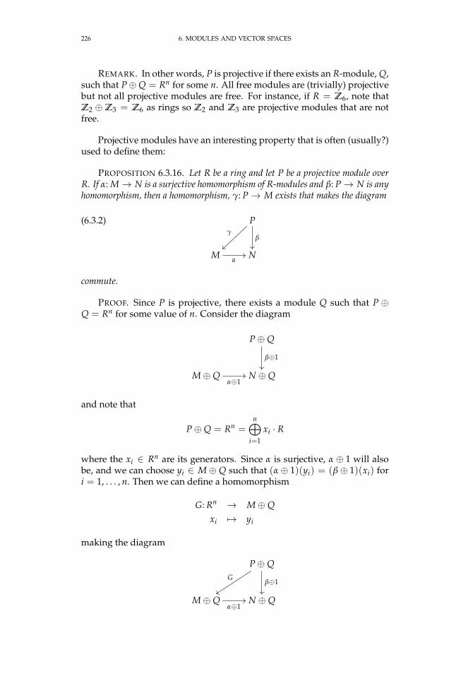
226 6. MODULES AND VECTOR SPACES
REMARK. In other words, P is projective if there exists an R-module, Q,such that P⊕Q = Rn for some n. All free modules are (trivially) projectivebut not all projective modules are free. For instance, if R = Z6, note thatZ2 ⊕Z3 = Z6 as rings so Z2 and Z3 are projective modules that are notfree.
Projective modules have an interesting property that is often (usually?)used to define them:
PROPOSITION 6.3.16. Let R be a ring and let P be a projective module overR. If α: M→ N is a surjective homomorphism of R-modules and β: P→ N is anyhomomorphism, then a homomorphism, γ: P→ M exists that makes the diagram
(6.3.2) P
β
γ
~~
Mα// N
commute.
PROOF. Since P is projective, there exists a module Q such that P ⊕Q = Rn for some value of n. Consider the diagram
P⊕Q
β⊕1
M⊕Qα⊕1// N ⊕Q
and note that
P⊕Q = Rn =n⊕
i=1
xi · R
where the xi ∈ Rn are its generators. Since α is surjective, α ⊕ 1 will alsobe, and we can choose yi ∈ M⊕ Q such that (α⊕ 1)(yi) = (β⊕ 1)(xi) fori = 1, . . . , n. Then we can define a homomorphism
G: Rn → M⊕Qxi 7→ yi
making the diagram
P⊕QG
yy
β⊕1
M⊕Qα⊕1// N ⊕Q
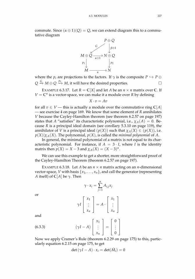
6.3. MODULES 227
commute. Since (α⊕ 1)(Q) = Q, we can extend diagram this to a commu-tative diagram
P⊕QG
yy
β⊕1
M⊕Qα⊕1//
p1
N ⊕Q
p2
Mα
// N
where the pi are projections to the factors. If γ is the composite P → P⊕Q G−→ M⊕Q
p1−→ M, it will have the desired properties.
EXAMPLE 6.3.17. Let R = C[X] and let A be an n× n matrix over C. IfV = Cn is a vector-space, we can make it a module over R by defining
X · v = Av
for all v ∈ V — this is actually a module over the commutative ring C[A]— see exercise 4 on page 169. We know that some element of R annihilatesV because the Cayley-Hamilton theorem (see theorem 6.2.57 on page 197)states that A “satisfies” its characteristic polynomial, i.e., χA(A) = 0. Be-cause R is a principal ideal domain (see corollary 5.3.10 on page 119), theannihilator of V is a principal ideal (p(X)) such that χA(X) ∈ (p(X)), i.e.p(X)|χA(X). The polynomial, p(X), is called the minimal polynomial of A.
In general, the minimal polynomial of a matrix is not equal to its char-acteristic polynomial. For instance, if A = 3 · I, where I is the identitymatrix then p(X) = X− 3 and χA(X) = (X− 3)n.
We can use this example to get a shorter, more straightforward proof ofthe Cayley-Hamilton Theorem (theorem 6.2.57 on page 197).
EXAMPLE 6.3.18. Let A be an n× n matrix acting on an n-dimensionalvector-space, V with basis x1, . . . , xn, and call the generator (representingA itself) of C[A] be γ. Then
γ · xi =n
∑j=1
Ai,jxj
or
γI
x1...
xn
= A ·
x1...
xn
and
(6.3.3) (γI − A)
x1...
xn
=
0...0
Now we apply Cramer’s Rule (theorem 6.2.29 on page 175) to this, partic-ularly equation 6.2.15 on page 175, to get
det (γI − A) · xi = det(Mi) = 0

228 6. MODULES AND VECTOR SPACES
where M = γI − A and Mi is the result of replacing the ith column of M bythe right side of equation 6.3.3 on the preceding page — zeroes. It followsthat det (γI − A) = χA(γ) annihilates all of the xi. If we get a matrix-representation (i.e., by replacing γ by A) we get a matrix that annihilatesall basis-elements of V, i.e., the zero-matrix.
EXERCISES.
1. If A ⊂ R is an ideal in a commutative ring, R, then A is also an R-module. Show that, if A is a free R-module, it must be of the form A = (x)where x ∈ R is a non-zero divisor.
2. Let f : M1 → M2 be a homomorphism of modules (over a commuta-tive ring, or left-modules over a noncommutative one). Suppose A ⊂ M1is a submodule and
f |A: A→ f (A)
Show that there is an induced map
f :M1
A→ M2
f (A)
6.3.2. Modules over principal ideal domains. When a ring is a PID, itturns out one can easily classify modules over it. Throughout this section,R will denote a PID — see definition 5.3.8 on page 119.
PROPOSITION 6.3.19. If S ⊂ A is a submodule of a free R-module, then S isfree. If rank(A) < ∞, then
rank(S) ≤ rank(A)
REMARK. Compare this with proposition 4.6.6 on page 61. The proof isessentially the same. If we had proved the current result first, we could’veregarded proposition 4.6.6 on page 61 as a corollary with R = Z.
EXAMPLE 6.3.20. Exercise 1 produces plenty of counterexamples if Ris not a PID. For instance, Z6 is free as a Z6-module, but the ideal (i.e.,submodule) 2Z6 = 0, 2, 4 is not because 3 · 2 = 3 · 4 = 0 ∈ Z6 so none ofthese can be free generators of 2Z6. The ideal (X, Y) ⊂ C[X, Y] is anothercounterexample.
REMARK. There’s a whole subfield of algebra that studies the extent towhich proposition 6.3.19 fails in general (among other things). It is calledAlgebraic K-theory — see [106].
PROOF. Let X be a free basis for A. By the Well Ordering Axiom of settheory (see axiom A.2.9 on page 461), we can order the elements of X
x1 x2 · · ·
6.3. MODULES 229
so that every subset of X has a minimal element. Note that this ordering iscompletely arbitrary — we only use the fact that such an ordering exists.
If s ∈ S, we have
s = ∑ rixi
— a unique finite sum, with ri ∈ R. Define the leading term, λ(s) = rαxα —the highest ordered term in the sum. Let Y ⊂ X be the set of basis elementsthat occur in these leading terms of elements of S. For each y ∈ Y, there isat least one s ∈ S whose leading term is r · y. Let
(6.3.4) I(y) = 0 ∪ r ∈ R|λ(s) = r · y for some s ∈ SIt is not hard to see that
I(y) ⊂ R
is an ideal — since λ(r′s) = r′λ(s). Since R is a PID, it follows that I(y) =(ry), and there exists a set of elements Sy ⊂ S whose leading terms are ryy.The Axiom of Choice (see theorem A.2.11 on page 461) implies that we canselect one such element for each y ∈ Y — i.e. we can define a function
f : Y → S
where f (y) is some (arbitrarily selected) element of Sy. We claim that theset
B = f (y)|y ∈ Yis a basis for S. We must demonstrate two things:
(1) the set B is linearly independent. This follows immediately from thefact that its leading terms are multiples of distinct basis elementsof A. Suppose we have a linear combination
n
∑i=1
riyi + H = 0
where H is the non-leading terms. Of those leading terms, one isordered the highest — say rαyα and it can never be canceled outby any other term. It follows that rα = 0 and a similar argumentapplied to the remaining terms eventually leads to the conclusionthat all of the coefficients are 0.
(2) the set B generates S. Suppose not and suppose g ∈ S \ 〈B〉 has theproperty that λ(g) = ry for r ∈ R and y ∈ Y is minimal (in theordering on X — axiom A.2.9 on page 461). Then r ∈ I(g) = (rg)so that r = r′ · rg and r′ · f (y) ∈ 〈B〉 also has leading term ry. Itfollows that
g− r′ · f (y) ∈ S \ 〈B〉has a leading term strictly lower than that of g — a contradiction.
We also get a form of the Chinese Remainder Theorem:
230 6. MODULES AND VECTOR SPACES
PROPOSITION 6.3.21. Let r1, . . . , rk be a set of elements of R such thatgcd(ri, rj) = 1 (see Proposition 5.3.6 on page 118) whenever i 6= j. Then
R(r1 · · · rk)
∼=k⊕
i=1
R(ri)
PROOF. The hypotheses imply that
(ri) + (rj) = R
whenever i 6= j and
(r1 · · · rk) =k⋂
i=1
(ri)
so the conclusion follows from exercise 12 on page 116.
LEMMA 6.3.22. Let r, s ∈ R with t = gcd(r, s). Let α, β ∈ R be such thatαr + βs = t. Then the matrix
A =
[α β−s/t r/t
]has inverse [
r/t −βs/t α
]and
A[
rs
]=
[t0
]If At is the transpose of A, then[
r s]
At =[
t 0]
REMARK. The existence of α and β follows from the fact that (r, s) =(t).
PROOF. Straightforward computation.
THEOREM 6.3.23. If M is a finitely generated R-module then
(6.3.5) M ∼= F⊕ R(g1)
⊕ · · · ⊕ R(gk)
where F is free and g1∣∣ g2
∣∣ · · · ∣∣ gk. The free submodule, F, and the R/(gi) areuniquely determined by M and are called its invariant factors.
REMARK. The proof is very similar to that of theorem 4.6.8 on page 62except that we do not have the Euclidean algorithm to simplify a matrix.Lemma 6.3.22 takes its place.
PROOF. Propositions 6.3.10 on page 223 and 6.3.19 on page 228 implythat
M ∼= GK

6.3. MODULES 231
where G and K are both free modules of respective ranks n and m ≤ n. Ifx1, . . . , xm is a free basis for K and y1, . . . , yn is one for G then
yi =n
∑j=1
ai,jxj
the m× n matrix A = [ai,j] expresses how K fits in G and the quotient. Weconsider ways of “simplifying” this matrix in such a way that the quotientG/K remains unchanged. Multiplication on the right by an invertible ma-trix corresponds to a change of basis for K and on the left a change of basisfor G. It follows that the quotient is unchanged. As in theorem 4.6.8 onpage 62, we do row-reduction, and then column-reduction.
We’ll call this part of our algorithm, Diagonalization:This consists of two phases: row-reduction and column-reduction.By permuting rows and columns, if necessary, assume a1,1 6= 0. If this
is impossible, we have a matrix of zeros and there is no work to be done.We will call the (1, 1) position in the matrix, the pivot.Now we scan down column 1.
(1) If a1,1|ak,1 with k > 1, we subtract (a1,1/ak,1)× row 1 from row k,replacing ak,1 by 0.
(2) If a1,1 - ak,1, perform two steps:(a) swap row k with row 2 so ak,1 becomes 0 and a2,1 becomes the
original value of ak,1,(b) apply lemma 6.3.22 on the facing page and left-multiply the
matrix A by a matrix whose first two rows and columns are
(6.3.6)[
α β−a2,1/δ a1,1/δ
]and whose remaining rows are the identity matrix. Here δ =gcd(a1,1, a2,1), α and β are such that αa1,1 + βa2,1 = δ. Sincethis matrix is invertible, it represents a basis change of K andhas no effect on the quotient.
The effect is8:
a1,1 → δ
a2,1 → 0ak,1 → 0
Repeating these operations for all lower rows ultimately clears all elementsof column 1 below a1,1 to 0. This completes row-reduction for column 1.
Now we do column-reduction on row 1, ultimately clearing out all el-ements to the right of a1,1 to 0. Here, we right-multiply the matrix by thetranspose of a matrix like that in equation 6.3.6.
After these steps, our matrix looks like[a1,1 00 M
]where M is an (m− 1)× (n− 1) matrix.
8Where the symbol ‘→’ means “is replaced by.”

232 6. MODULES AND VECTOR SPACES
After recursively carrying out our algorithm above on this and thesmaller sub-matrices that result, we get the diagonal form:
a1,1 0 0 · · · 00 a2,2 0 · · · 0...
.... . . · · · ...
0 0 0 · · · 0
where all off-diagonal entries are 0 and we have n − m columns of 0’s onthe right. This matrix means that the new bases for K and F satisfy
yi = ai,i · xi
for 1 ≤ i ≤ m. This completes the phase of the algorithm called diagonal-ization.
Now we may run into the problem ai,i - ai+1,i+1. This is easily resolved:just add column i + 1 to column i to give[
ai,i 0ai+1,i+1 ai+1,i+1
]Left multiplication by [
α β−ai+1,i+1/δ ai,i/δ
]where αai,i + βai+1,i+1 = δ = gcd(ai,i, ai+1,i+1) (as in lemma 6.3.22 onpage 230), gives [
δ βai+1,i+10 ai,i ai+1,i+1/δ
]At this point, we subtract (βai+1,i+1/δ)× column i from column i+ 1 to get[
δ 00 ai,i ai+1,i+1/δ
]and we have δ
∣∣ (ai,i ai+1,i+1/δ) = lcm(ai,i, ai+1,i+1). Notice that the productof these diagonal entries is the same as before. On the other hand, thenumber of distinct prime factors in δ must be strictly less than those in ai,iand ai+1,i+1 (equality only occurs if ai,i and ai+1,i+1 have the same primefactors).
Note that this operation shifts prime factors to the right and down.After a finite number of steps, a1,1 must stabilize (i.e. remain constant overiterations of this process) since it has a finite number of prime factors. Onecan say the same of a2,2 as well. Eventually the entire list of elements
a1,1, . . . , am,mmust stabilize, finally satisfying the condition
a1,1∣∣ · · · ∣∣ am,m
each nonzero entry ai,i results in a direct summand R/(ai,i), if ai,i isnot a unit, and 0 otherwise.
each column of zeros contributes a direct summand of R to F inequation 6.3.5 on page 230.

6.3. MODULES 233
EXERCISES.
3. In theorem 6.3.23 on page 230 why are F and the invariant factorsuniquely determined by M?
4. If R is a PID and A is an m× n matrix over R, there exists an invert-ible m×m matrix, S, and an invertible n× n matrix, T, such that
SAT
is a diagonal matrix with the property that the diagonal entries di satisfydi∣∣ di+1 for all i. This is called the Smith Normal Form of A and the proof
of theorem 6.3.23 on page 230 gives an algorithm for computing it. Thematrices S and T are computed by keeping careful track of the steps inthe algorithm (i.e., adding a row to another is multiplication by a suitableelementary matrix). Find the Smith normal form of the matrix (over Z): 2 4 4
−6 6 1210 −4 −16
6.3.3. Jordan Canonical Form. In this section, we will apply a knowl-edge of rings and modules to find a standard form for matrices. It is well-known that not all matrices can be diagonalized — for instance
B =
[1 10 1
]has a single eigenvalue of 1 and eigenvector[
10
]which doesn’t span C2. All matrices can be put into Jordan Canonical Form,which is as close as one can get to diagonalization.
Marie Ennemond Camille Jordan (1838 – 1922) was a French mathematicianknown for (besides Jordan Canonical Form) the Jordan Curve Theorem andthe Jordan–Hölder theorem (see theorem 4.9.5 on page 85), and his influen-tial series of books, Cours d’analyse.
PROPOSITION 6.3.24. Let V be an n-dimensional vector-space over an C. IfA: V → V is a linear transformation, we can define an action of C[X] on V as inexample 6.3.17 on page 227:
X · v = Av
234 6. MODULES AND VECTOR SPACES
for all v ∈ V. Then, as C[X]-modules
(6.3.7) V ∼= C[X]
(p1(X))⊕ · · · ⊕ C[X]
(pk(X))
where p1(X)∣∣ · · · ∣∣ pk(X) where pk(X) is the minimal polynomial of V (see ex-
ample 6.3.17 on page 227),
k
∑i=1
deg pi(X) = n
andk
∏i=1
pi(X) = χA(X)
the characteristic polynomial of A.
PROOF. Equation 6.3.7 follows immediately from theorem 6.3.23 onpage 230 since C[X] is a PID (see corollary 5.3.10 on page 119). That pk(X)is the minimal polynomial of V follows from the fact that it is the lowest-degree polynomial that annihilates the right side of equation 6.3.7. Thestatement regarding dimensions follows from
dimC[X]
(p(X))= deg p(X)
To prove the final statement, note that each of the summands
C[X]
(pi(X))
represents an A-invariant subspace of V so there exists a basis of V forwhich A is a block-matrix
A =
A1 0 · · · 0
0. . . 0
.... . .
...0 · · · 0 Ak
where the Ai are the restrictions of A to each of these invariant subspaces(in this basis!). We claim that, in the subspace
C[X]
(pi(X))
the characteristic polynomial of Ai is just pi(X), same as the minimumpolynomial. This is because they have the same degree, and one must di-vide the other. The conclusion follows from exercise 16 on page 199.
COROLLARY 6.3.25. Under the assumptions of proposition 6.3.24 on the pre-ceding page we have an isomorphism of C[X]-modules
V ∼= C[X]
(X− λ1)α1⊕ · · · ⊕ C[X]
(X− λm)αm
6.3. MODULES 235
where λ1, . . . , λm are the eigenvalues of A andm
∑i=1
αi = n
Each summandC[X]
(X− λi)αi
is isomorphic to an A-invariant subspace, Vi, of V and there exists a basis of V inwhich A is a block matrix
A =
A1 0 · · · 0
0. . . 0
.... . .
...0 · · · 0 Am
where
Ai = A|Vi ⊂ V
PROOF. Simply factor the pj(X) in proposition 6.3.24 on page 233into powers of linear factors (possible in C). These factors are pairwise rela-tively prime to each other so the conclusion follows from proposition 6.3.21on page 230.
Our final conclusion is
THEOREM 6.3.26. Let V be an n-dimensional vector-space over an C. IfA: V → V is a linear transformation, there exists a basis for V such that A is ablock-matrix
A =
Jα1(λ1) 0 · · · 0
0. . . 0
.... . .
...0 · · · 0 Jαm(λm)
where the block
(6.3.8) Jα(λ) =
λ 0 0 · · · 0
1 λ. . . . . .
...
0 1. . . . . . 0
... · · · . . . λ 00 · · · 0 1 λ
is an α× α matrix with λ on the main diagonal, 1’s in the diagonal below it andzeros elsewhere. It is called a Jordan Block.
REMARK. Note that J1(λ) = [λ]. If all the eigenvalues are distinct, theJordan blocks are all of size 1, and we get the usual diagonalized form of thematrix,
This representation is called the Jordan Canonical Form of the matrix A.The form given here is the transpose of the usual Jordan block, due to ourapplying the matrix A on the left.
236 6. MODULES AND VECTOR SPACES
PROOF. We need to show that
Ai: Vi =C[X]
(X− λi)αi→ C[X]
(X− λi)αi
in corollary 6.3.25 on page 234 can be put in the form Jαi (λi). We claim thatthe image of
e1 = 1, e2 = X− λi, . . . , eαi = (X− λi)αi−1
in Vi is a basis. The ej must be linearly independent since a linear rela-tion would imply that a polynomial of degree αi − 1 could annihilate Vi —contradicting the idea that (X− λi)
αi is its minimal polynomial. The ei alsospan Vi since all linear combinations of the Xi can be written in terms ofthem. The matrix Ai acts like multiplication by X in the quotient
C[X]
(X− λi)αi
and it is not hard to see that X · ej = λiej + ej+1 for j = 1, . . . , αi − 1 andX · eαi = λieαi . Written as a matrix, this is precisely equation 6.3.8 on thepreceding page.
We will do some computations. Let
A =
−5 −1 −2 −1 −4−1 3 2 −1 021 2 5 4 1132 4 8 7 18
0 0 0 0 1
The characteristic polynomial is
χA(λ) = det(λI − A)
= λ5 − 11λ4 + 47λ3 − 97λ2 + 96λ− 36
= (λ− 1) · (λ− 3)2 · (λ− 2)2
So its eigenvalues are 1, 2, and 3.Eigenvalue 1. We compute the nullspace of A− I. This turns out to be
the span of
v1 =
1−32−3−1
Eigenvalue 2. The nullspace of A− 2I is the span of
1−1−1−40
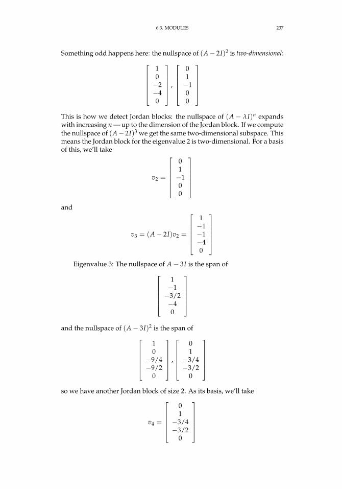
6.3. MODULES 237
Something odd happens here: the nullspace of (A− 2I)2 is two-dimensional:10−2−40
,
01−100
This is how we detect Jordan blocks: the nullspace of (A − λI)n expandswith increasing n — up to the dimension of the Jordan block. If we computethe nullspace of (A− 2I)3 we get the same two-dimensional subspace. Thismeans the Jordan block for the eigenvalue 2 is two-dimensional. For a basisof this, we’ll take
v2 =
01−100
and
v3 = (A− 2I)v2 =
1−1−1−40
Eigenvalue 3: The nullspace of A− 3I is the span of
1−1−3/2−40
and the nullspace of (A− 3I)2 is the span of
10−9/4−9/2
0
,
01−3/4−3/2
0
so we have another Jordan block of size 2. As its basis, we’ll take
v4 =
01−3/4−3/2
0
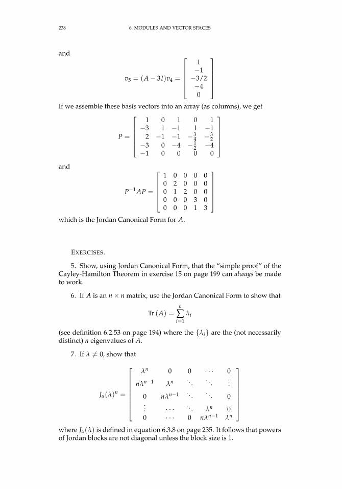
238 6. MODULES AND VECTOR SPACES
and
v5 = (A− 3I)v4 =
1−1−3/2−40
If we assemble these basis vectors into an array (as columns), we get
P =
1 0 1 0 1−3 1 −1 1 −1
2 −1 −1 − 34 − 3
2−3 0 −4 − 1
2 −4−1 0 0 0 0
and
P−1 AP =
1 0 0 0 00 2 0 0 00 1 2 0 00 0 0 3 00 0 0 1 3
which is the Jordan Canonical Form for A.
EXERCISES.
5. Show, using Jordan Canonical Form, that the “simple proof” of theCayley-Hamilton Theorem in exercise 15 on page 199 can always be madeto work.
6. If A is an n× n matrix, use the Jordan Canonical Form to show that
Tr (A) =n
∑i=1
λi
(see definition 6.2.53 on page 194) where the λi are the (not necessarilydistinct) n eigenvalues of A.
7. If λ 6= 0, show that
Jα(λ)n =
λn 0 0 · · · 0
nλn−1 λn . . . . . ....
0 nλn−1 . . . . . . 0... · · · . . . λn 00 · · · 0 nλn−1 λn
where Jα(λ) is defined in equation 6.3.8 on page 235. It follows that powersof Jordan blocks are not diagonal unless the block size is 1.
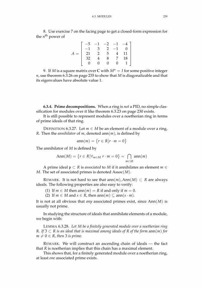
6.3. MODULES 239
8. Use exercise 7 on the facing page to get a closed-form expression forthe nth power of
A =
−5 −1 −2 −1 −4−1 3 2 −1 021 2 5 4 1132 4 8 7 18
0 0 0 0 1
9. If M is a square matrix over C with Mn = I for some positive integer
n, use theorem 6.3.26 on page 235 to show that M is diagonalizable and thatits eigenvalues have absolute value 1.
6.3.4. Prime decompositions. When a ring is not a PID, no simple clas-sification for modules over it like theorem 6.3.23 on page 230 exists.
It is still possible to represent modules over a noetherian ring in termsof prime ideals of that ring.
DEFINITION 6.3.27. Let m ∈ M be an element of a module over a ring,R. Then the annihilator of m, denoted ann(m), is defined by
ann(m) =
r ∈ R∣∣r ·m = 0
The annihilator of M is defined by
Ann(M) =
r ∈ R∣∣∀m∈M r ·m = 0
=
⋂m∈M
ann(m)
A prime ideal p ⊂ R is associated to M if it annihilates an element m ∈M. The set of associated primes is denoted Assoc(M).
REMARK. It is not hard to see that ann(m), Ann(M) ⊂ R are alwaysideals. The following properties are also easy to verify:
(1) If m ∈ M then ann(m) = R if and only if m = 0.(2) If m ∈ M and s ∈ R, then ann(m) ⊆ ann(s ·m).
It is not at all obvious that any associated primes exist, since Ann(M) isusually not prime.
In studying the structure of ideals that annihilate elements of a module,we begin with:
LEMMA 6.3.28. Let M be a finitely generated module over a noetherian ringR. If I ⊂ R is an ideal that is maximal among ideals of R of the form ann(m) form 6= 0 ∈ R, then I is prime.
REMARK. We will construct an ascending chain of ideals — the factthat R is noetherian implies that this chain has a maximal element.
This shows that, for a finitely generated module over a noetherian ring,at least one associated prime exists.
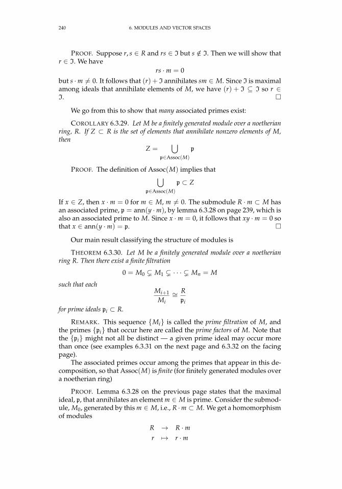
240 6. MODULES AND VECTOR SPACES
PROOF. Suppose r, s ∈ R and rs ∈ I but s /∈ I. Then we will show thatr ∈ I. We have
rs ·m = 0
but s ·m 6= 0. It follows that (r) + I annihilates sm ∈ M. Since I is maximalamong ideals that annihilate elements of M, we have (r) + I ⊆ I so r ∈I.
We go from this to show that many associated primes exist:
COROLLARY 6.3.29. Let M be a finitely generated module over a noetherianring, R. If Z ⊂ R is the set of elements that annihilate nonzero elements of M,then
Z =⋃
p∈Assoc(M)
p
PROOF. The definition of Assoc(M) implies that⋃p∈Assoc(M)
p ⊂ Z
If x ∈ Z, then x ·m = 0 for m ∈ M, m 6= 0. The submodule R ·m ⊂ M hasan associated prime, p = ann(y ·m), by lemma 6.3.28 on page 239, which isalso an associated prime to M. Since x ·m = 0, it follows that xy ·m = 0 sothat x ∈ ann(y ·m) = p.
Our main result classifying the structure of modules is
THEOREM 6.3.30. Let M be a finitely generated module over a noetherianring R. Then there exist a finite filtration
0 = M0 ( M1 ( · · · ( Mn = M
such that eachMi+1
Mi∼= R
pifor prime ideals pi ⊂ R.
REMARK. This sequence Mi is called the prime filtration of M, andthe primes pi that occur here are called the prime factors of M. Note thatthe pi might not all be distinct — a given prime ideal may occur morethan once (see examples 6.3.31 on the next page and 6.3.32 on the facingpage).
The associated primes occur among the primes that appear in this de-composition, so that Assoc(M) is finite (for finitely generated modules overa noetherian ring)
PROOF. Lemma 6.3.28 on the previous page states that the maximalideal, p, that annihilates an element m ∈ M is prime. Consider the submod-ule, M0, generated by this m ∈ M, i.e., R ·m ⊂ M. We get a homomorphismof modules
R → R ·mr 7→ r ·m

6.3. MODULES 241
Since p is in the kernel, we get a homomorphism of R-modules
g: R/p→ R ·mSince p is maximal, any element in the kernel of g must lie in p, so
Rp∼= R ·m = M1
Now, form the quotient M/M1 and carry out the same argument, forminga submodule M′2 ⊂ M/M1 and its inverse image over the projection
M→ M/M1
is M2. We continue this process over and over until we get to 0. It mustterminate after a finite number of steps because M is finitely generated overa noetherian ring (see definition 6.3.11 on page 224).
EXAMPLE. If M = Z60 is regarded as a module over Z, then a maximalideal is of the form (p) ⊂ Z for some prime p. For instance, (2) annihilatesM1 = 30 ·Z60 and M/M1 = Z30. The ideal (2) annihilates M2 = 15 ·Z30and we get M1/M2 = Z15. The ideal (3) annihilates 5 ·Z15 and we aredone (the final quotient is Z5). We can lift these modules up into M to get
0 ⊂ 30 ·Z60 ⊂ 15 ·Z60 ⊂ 5 ·Z60 ⊂ Z60
with prime factors, Z2, Z2, Z3 and Z5, respectively.
EXAMPLE 6.3.31. Returning to example 6.3.17 on page 227, let p ⊂ R bea prime ideal that annihilates an element v ∈ V. Then p = (X − λ) and λmust be an eigenvalue. The element, v, annihilated by p is the correspondingeigenvector. A simple induction shows that all of the prime ideals we get inthe prime decomposition of V are of the form (X − λi) where the λi runthrough the eigenvalues of A.
Here’s a much more detailed example:
EXAMPLE 6.3.32. Let R = C[X, Y]/a where
(6.3.9) a = (Y3, XY + Y, X2 + Y2 − 1) ⊂ C[X, Y]
Lemma 5.2.9 on page 114 implies that the prime ideals of R are imagesunder the projection
p: C[X, Y]→ C[X, Y]/a = R
of the prime ideals of C[X, Y] that contain a. We will skip ahead and usetheorem 12.2.3 on page 416 to conclude that the prime ideals of C[X, Y] areeither of the form ( f (X, Y)) for some irreducible polynomial, f , or of theform (X − α, Y − β) for α, β ∈ C. We reject the possibility of a principalideal because f (X, Y)|Y3 implies that f (X, Y) = Y but that does not divideX2 + Y2 − 1.
If a ⊂ (X− α, Y− β), then equations like
p1(X, Y)(X− α) + q1(X, Y)(Y− β) = Y3
p2(X, Y)(X− α) + q2(X, Y)(Y− β) = XY + Y
p3(X, Y)(X− α) + q3(X, Y)(Y− β) = X2 + Y2 − 1
242 6. MODULES AND VECTOR SPACES
must hold, for some pi, qi ∈ k[X, Y]. The top equation forces β = 0 (i.e., setX = α). This also satisfies the second equation since we can set p2 = 0 andq2 = X + 1. The bottom equation becomes
p3(X, Y)(X− α) + q3(X, Y)Y = X2 + Y2 − 1
We simplify this by setting q3 = Y and subtracting to get
p3(X, Y)(X− α) = X2 − 1 = (X− 1)(X + 1)
which implies that α = ±1. It follows that P1 = (X − 1, Y) and P2 =(X + 1, Y) are the only two ideals of the form (X− α, Y− β) that contain a.
Let x, y ∈ R be the images of X and Y, respectively under the projection,p above — they clearly generate R as a ring. Then the prime ideals of R arep1 = (x− 1, y) and p2 = (x + 1, y). In addition, lemma 5.2.10 on page 114implies that
Rpi
=C[X, Y]
Pi= C
for i = 1, 2.Now we will compute a prime filtration of R as a module over itself.
Since y2 · p2 = 0, we regard y2 · R as a candidate for R1. Let us computewhat happens to 1, x, y when we multiply by y2
y2 · 1 = y2
y2 · x = y · (−y) = −y2 because of the relation xy + y = 0in equation 6.3.9
y2 · y = 0 because of the relation y3 = 0in equation 6.3.9
It follows that y2 · R = C · y2 = C and we get an isomorphism
R1 = y2 · R =Rp2
= C · y2
Following the proof of theorem 6.3.30 on page 240, we form the quotient
(6.3.10) R′ =RR1
=k[X, Y]
(Y3, Y2, XY + Y, X2 + Y2 − 1)
=k[X, Y]
(Y2, XY + Y, X2 − 1)
— where we eliminated Y3 since (Y3) ⊂ (Y2) and eliminated the Y2 termfrom X2 + Y2 − 1. Notice that p2 · y = 0. This suggests using y · R′ asour second prime quotient. As before, we enumerate the effect of y· on thegenerators of R′:
y · 1 = y
y · x = −y because of the relation xy + y = 0in equation 6.3.10
y · y = 0 because of the relation y2 = 0in equation 6.3.10
6.3. MODULES 243
Again, we conclude that y · R′ = C, generated by y, and get
Rp= y · R′ = C · y
and we take the inverse image of y · R′ over the projection R→ R/R1 = R′
to get R2 = y · R and a partial prime filtration
0 ( y2 · R ( y · RContinuing, we form the quotient again
(6.3.11) R′′ =R′
C · y =k[X, Y]
(Y2, Y, XY + Y, X2 − 1)=
k[X, Y](Y, X2 − 1)
and notice that p2 · (x− 1) = 0. Computing (x− 1) · R′′ gives
(x− 1) · 1 = (x− 1)
(x− 1) · x = x2 − x = −(x− 1) because of the relationx2 − 1 = 0 in equation 6.3.11
(x− 1) · y = 0 because of the relation y = 0in equation 6.3.11
so (x− 1) · R′′ = C, generated by x− 1 and
Rp2
= (x− 1) · R′′ = C · (x− 1)
and this lifts to (x− 1) · R ⊂ R. In the final step, we get
R′′′ =R′′
(x− 1) · R′′ =k[X, Y]
(Y, X2 − 1, X− 1)=
k[X, Y](Y, X− 1)
=Rp1
(since (X2 − 1) ⊂ (X− 1)), so we get our complete prime filtration
0 ( y2 · R ( y · R ( (x− 1) · R ( R
The prime p2 occurs three times, and the last factor involves the prime p1.
Another interesting and useful result is called Nakayama’s Lemma —it has a number of applications to algebraic geometry and other areas ofalgebra:
LEMMA 6.3.33. Let M be a finitely-generated module over a commutativering, R. If a ⊂ R is an ideal with the property that
a ·M = M
then there exists an element r ∈ R such that r ≡ 1 (mod a) and
r ·M = 0
REMARK. This result is named after Tadashi Nakayama who intro-duced it in [78]. Special cases of it had been discovered earlier by Krull,and Azumaya had published the general case in [7] before Nakayama’s pa-per. The version for noncommutative rings is called the Krull-AzumayaTheorem.
244 6. MODULES AND VECTOR SPACES
PROOF. Let m1 . . . , mk denote the generators of M over R so
M = R ·m1 + · · ·+ R ·mk
Since a ·M = M, we have
mi =k
∑j=1
Ai,jmj
for some k× k matrix A = [Ai,j] with entries in a. Subtracting givesn
∑j=1
(δi,j − Ai,j)mj = 0
where δi,j is the (i, j)th entry of the identity matrix, or
δi,j =
1 if i = j0 otherwise
or
(I − A)
m1...
mk
= 0
Cramer’s Rule (theorem 6.2.29 on page 175) implies that
det(I − A)mi = Ci = 0
for all i, where Ci is the determinant of the matrix one gets by replacing theithcolumn by 0’s. So r ∈ R in the statement of the lemma is just det(I − A).
We claim that det(I − A) = 1 + a for some a ∈ a. The determinant ofI − A is what one gets from the characteristic polynomial pA(x) by settingx = 1. Since the characteristic polynomial is monic, one term is equal to 1and the remaining terms are linear combinations of elements of a.
Here’s a consequence of Nakayama’s lemma (a special case of the KrullIntersection Theorem — see [63]):
LEMMA 6.3.34. Let m ⊂ R be a maximal ideal of a noetherian ring, R or anarbitrary ideal of a noetherian domain. Then
∞⋂j=1
mj = (0)
PROOF. Call this infinite intersection b. Since R is noetherian, b isfinitely generated as a module over R. Since
m · b = b
Nakayama’s Lemma ( 6.3.33 on the previous page) implies that b is annihi-lated by an element x ∈ R such that x ≡ 1 (mod m) and such an elementis a unit so b = (0).
If R is an integral domain and m is an arbitrary ideal, x 6= 0 and x · b = 0implies b = 0 since R has no zero-divisors.
We also get a result for local rings:
6.3. MODULES 245
COROLLARY 6.3.35. Let R be a local ring (see definition 5.2.8 on page 113)with unique maximal ideal m ⊂ R. If M is an R-module with the property that
m ·M = M
then M = 0.
PROOF. Nakayama’s lemma implies that there exists r ∈ R such thatr ≡ 1 (mod m) and r ·M = 0. Since R is a local ring, m is the only maximalideal and therefore equal to the intersection of all maximal ideals. Exer-cise 10 on page 116 implies that this r is a unit, i.e., has a multiplicativeinverse, s ∈ R. Consequently
r ·M = 0 =⇒ s · r ·M = 0 =⇒ 1 ·M = 0
and the conclusion follows.
EXERCISES.
10. If0→ U → V →W → 0
is a short exact sequence of vector-spaces, show that
dim V = dim U + dim W
11. Prove this basic result in linear algebra:A vector-space over an infinite field cannot be a finiteunion of proper subspaces.
12. Give a counterexample to statement in exercise 11 if the field ofdefinition is finite.
13. If P and M are R-modules, with P projective and
f : M→ P
is a surjective homomorphism, show that there exists a homomorphismg: P→ M such that f g = 1: P→ P.
14. If0→ M1 → M2 → M3 → 0
is a short exact sequences of modules over a ring R, show that
Ann(M1) ·Ann(M3) ⊂ Ann(M2) ⊂ Ann(M1) ∩Ann(M3)
15. Let
0→ Uq−→ V
p−→W → 0be a short exact sequence of modules, and suppose there exists a homo-morphism
h: W → Vsuch that p h = 1: W → W (such short exact sequences are said to be splitand h is called a splitting map). Show that there exists an isomorphism
V ∼= U ⊕W
246 6. MODULES AND VECTOR SPACES
16. Let
0→ Uq−→ V
p−→ P→ 0be a short exact sequence of modules, and suppose that P is a projectivemodule. Show that there exists an isomorphism
V ∼= U ⊕ P
6.4. Rings and modules of fractions
We begin by defining multiplicative sets:
DEFINITION 6.4.1. A multiplicative set, S, is a set of elements of a ring,R that:
(1) contains 1(2) is closed under multiplication.
Our main application of multiplicative sets will be in constructing ringsand modules of fractions in section 6.4. We need this concept here, toprove 12.2.8 on page 417.
EXAMPLE. For instance, if p ⊂ R is a prime ideal, then S = R \ p is amultiplicative set.
We have a kind of converse to this:
PROPOSITION 6.4.2. If S ⊂ R is a multiplicative set in a commutative ringwith S−1R 6= 0, then any ideal I ⊂ R with I ∩ S = ∅ that is maximal withrespect to this property is prime.
REMARK. “Maximal with respect to this property” means that, givenany other ideal J with J ∩ S = ∅ and I ⊂ J, then I = J — i.e. I is notproperly contained in J.
Such a maximal ideal always exists, by Zorn’s Lemma ( A.2.12 onpage 462).
PROOF. Let I be such a maximal ideal and assume it is not prime. Thethere exist a, b ∈ R such that ab ∈ I and a /∈ I and b /∈ I. Then (a+I)∩ S 6=∅ and (b + I) ∩ S 6= ∅. Let s1 ∈ (a + I) ∩ S and s2 ∈ (b + I) ∩ S. Then
s1s2 ∈ (a + I)(b + I) ⊂ ab + aI+ bI+ I2 ⊂ I
which is a contradiction.
Given a multiplicative set, we can define the corresponding ring of frac-tions:
DEFINITION 6.4.3. Let M be a module over a ring, R, and let S ⊂ R be amultiplicative set. Then the module S−1M consists of pairs (s, m) ∈ S×M,usually written m/s, subject to the relation
m1
s1≡ m2
s2
6.4. RINGS AND MODULES OF FRACTIONS 247
if u · (s2 ·m1− s1 ·m2) = 0 for some u ∈ S and m1, m2 ∈ M. We make S−1Ma module by defining:
m1
s1+
m2
s2=
s2 ·m1 + s1 ·m2
s1 · s2
r · m1
s1=
r ·m1
s1
for all m1, m2 ∈ M, s1, s2 ∈ S, and r ∈ R.There exists a canonical homomorphism f : M→ S−1M that sends m ∈
M to m/1 ∈ S−1M.If M = R as a module over itself, then S−1R is a ring with multiplica-
tion defined byr1
s1· r2
s2=
r1 · r2
s1 · s2for all r1, r2 ∈ R and s1, s2 ∈ S.
REMARK. The kernel of the canonical map M → S−1M consists ofelements of M that are annihilated by elements of S. If R is an integraldomain, the map R→ S−1R is injective.
This construction has a universal property described inproposition 10.4.8 on page 351.
PROPOSITION 6.4.4. If a multiplicative set S ⊂ R contains elements s1, s2with the property that s1s2 = 0, then S−1M = 0, for any R-module, M.
PROOF. Suppose m ∈ M. We claim thatm1
=01∈ S−1M
In order for this to be true, we must have
s(m− 0) = 0
for some s ∈ S. But the fact that s1s2 = 0 implies that 0 ∈ S and we can justset
0(m− 0) = 0
DEFINITION 6.4.5. Let R be a ring and let h ∈ R. ThenSh = 1, h, h2, . . . is a multiplicative subset of A and we defineRh = S−1
h R.
REMARK. Every element of Rh can be written in the form a/hm and
ahm =
bhn ⇔ hJ(ahn − bhm) = 0
for some integer J ≥ 0.
LEMMA 6.4.6. For any ring A and h ∈ A, the map
∑ aixi 7→∑ai
hi
defines an isomorphismA[X]/(1− hX)→ Ah
248 6. MODULES AND VECTOR SPACES
PROOF. If h = 0, both rings are zero, so assume h 6= 0. In the ring A′ =A[X]/(1− hX), 1 = hX so h is a unit. Let α: A→ B be a homomorphism ofrings that α(h) is a unit in B.
The homomorphism
∑ aiXi 7→∑ α(ai)α(h)−i: A[X]→ B
factors through A′ because 1− hX 7→ 1− α(a)α(h)−1 = 0.Because α(h) is a unit in B, this is the unique extension of α to A′. There-
fore A′ has the same universal property as Ah so the two are uniquely iso-morphic.
When h|h′ so h′ = hg, there is a canonical homomorphismab7→ ag
h′: Ah → Ah′
so the rings Ah form a direct system indexed by the set S.
PROPOSITION 6.4.7. Suppose A is a ring and S ⊂ A is a multiplicative set.Then:
If S ⊂ A and b ⊂ A is an ideal, then S−1b is an ideal in S−1 A. If b contains any element of S, then S−1b = S−1 A.
It follows that
COROLLARY 6.4.8. The ideals in S−1 A are in a 1-1 correspondence with theideals of A that are disjoint from S.
DEFINITION 6.4.9. If p ⊂ A is a prime ideal, then S = A \ p is a multi-plicative set. Define Ap = S−1 A.
REMARK. Since any ideal b * p intersects S, it follows that S−1p is theunique maximal ideal in S−1 A.
S−1 A is, therefore, a local ring (a ring with a unique maximal ideal). Theword “local” is motivated by algebraic geometry (where it corresponds tothe geometric concept of “local”).
If a ring is not an integral domain, it has no field of fractions. Never-theless we can define a “closest approximation” to it
DEFINITION 6.4.10. If R is a ring and S is the set of non-zero-divisorsof R then
Q(R) = S−1R
is called the total quotient ring of R.
REMARK. If R is an integral domain, Q(R) is just the field of fractionsof R.
6.5. INTEGRAL EXTENSIONS OF RINGS 249
EXERCISES.
1. Suppose R is a ring with a multiplicative set S and a · s = 0 for a ∈ Rand s ∈ S. Show that
a1= 0 ∈ S−1R
2. Use the results of proposition 5.4.2 on page 122 to show that if R isnoetherian, so is S−1R for any multiplicative set S.
3. If R and S are rings, show that Q(R × S) = Q(R) × Q(S). Here,R× S is the ring of pairs (r, s) with pairwise addition and multiplication:
(r1, s1) + (r2, s2) = (r1 + r2, s1 + s2)
(r1, s1) · (r2, s2) = (r1 · r2, s1 · s2)
4. If R is a ring and M is an R-module, show that an element m ∈ Mgoes to 0 in all localizations Ma, where a ⊂ R runs over the maximal idealsof R if and only if m = 0.
5. If R is a ring and M is an R-module, show that Ma = 0 for allmaximal ideals a ⊂ R if and only if M = 0.
6. Suppose k is a field and R = k[[X]] is the ring of power-series in X(see definition 5.1.7 on page 109). If F = k((X)), the field of fractions of R,show that every element of F can be written in the form
Xα · rfor some α ∈ Z and some r ∈ R.
6.5. Integral extensions of rings
The theory of integral extensions of rings is crucial to algebraic numbertheory and algebraic geometry. It considers the question of “generalizedintegers:”
If Z ⊂ Q is the subring of integers, what subring, R ⊂Q[√
2], is like its “ring of integers”?
DEFINITION 6.5.1. If A ⊂ K is the inclusion of an integral domain in afield, x ∈ K will be called integral over A if it satisfies an equation
xj + a1xj−1 + · · ·+ ak = 0 ∈ A
with the ai ∈ A (i.e., is a root of a monic polynomial).
REMARK. For instance, consider Z ⊂ Q. The only integral elementsover Z are in Z itself.
In the case of Z ⊂ Q(i), we get integral elements n1 + n2 · i wheren1, n2 ∈ Z — the ring of Gaussian Integers.
PROPOSITION 6.5.2. Let R ⊂ S be integral domains. The following state-ments are equivalent
250 6. MODULES AND VECTOR SPACES
(1) An element s ∈ S is integral over R(2) R[s] is a finitely-generated R-module (see definition 6.3.8 on page 223).(3) s ∈ T for some subring of S with R ⊆ T ⊆ S and T is a finitely-
generated R-module.
REMARK. Note that being finitely generated as a module is very dif-ferent from being finitely generated as a ring or field. For instance R[X] isfinitely generated as a ring over R but, as a module, it is
∞⊕n=0
R · Xn
PROOF. 1 =⇒ 2. If s is integral over R, then
sn + an−1sn−1 + · · ·+ a0 = 0
with the ai ∈ R, sosn = −an−1sn−1 − · · · − a0
This means that R[s] — the ring of polynomials in s will only have polyno-mials of degree < n, so R[s] will be finitely generated as a module over R.Compare this argument to that used in proposition 7.2.2 on page 264.
2 =⇒ 3. Just set T = R[s].3 =⇒ 1. Suppose that t1, . . . , tn ∈ T is a set of generators of T as an
R-module. Then
sti =n
∑j=1
Ai,jtj
for some n× n matrix A, son
∑j=1
(δi,js− Ai,j)tj = 0
where
δi,j =
1 if i = j0 otherwise
Cramer’s Rule ( 6.2.29 on page 175) implies that
det(sI − A)ti = Ci = 0
for all i, where Ci is the determinant of the matrix one gets by replacing theithcolumn by 0’s. It follows that s is a root of the monic polynomial
det(XI − A) = 0 ∈ R[X]
DEFINITION 6.5.3. If R ⊆ S is an inclusion of integral domains andevery element of S is integral over R, then S will be said to be integral overR.
REMARK. It is not hard to see that this property is preserved in quo-tients. If a ⊂ S is an ideal then S/a will be integral over R/a ∩ R becausethe monic polynomials satisfied by every element of S over R will map tomonic polynomials in the quotients.
6.5. INTEGRAL EXTENSIONS OF RINGS 251
COROLLARY 6.5.4. Let f : R → S be an integral extension of integral do-mains. If a ⊂ R is a proper ideal, then so is a · S ⊂ S.
PROOF. We will prove the contrapositive: If a · S = S, then a = R.The statement that a · S = S and Nakayama’s Lemma 6.3.33 on page 243imply that there exists r ∈ R with r ≡ 1 (mod a) with r · S = 0. Since Sis an integral domain, we must have r = 0 to 0 ≡ 1 (mod a) or 1 ∈ a, soa = R.
PROPOSITION 6.5.5. Suppose R ⊆ S are integral domains and let s, t ∈ S.Then:
(1) If s and t are integral over R, so are t± s and st. Consequently integralelements over R form a ring.
(2) Let T be a commutative ring with S ⊆ T. If T is integral over S and Sis integral over R, then T is integral over R.
PROOF. If s and t are integral over R, let
R[s] = Rs1 + · · ·+ Rsk
R[t] = Rt1 + · · ·+ Rt`as R-modules. Then
R[s, t] = Rs1 + · · ·+ Rsk(6.5.1)+Rt1 + · · ·+ Rt`
+k,`
∑i=1,j=1
Rsitj
which contains s± t and st and is still a finitely generated R-module. Thisproves the first statement.
To prove the second statement, suppose t ∈ T satisfies the monic poly-nomial
tk + sk−1tk−1 + · · ·+ s0 = 0
with si ∈ S, and S[t] is a finitely generated S-module. Since S is integralover R, R[si] is a finitely-generated R-module, and so is
R′ = R[s0, . . . , sk−1]
— equation 6.5.1 gives some ideal of how one could obtain a finite setof generators. The element t is also monic over R′, so R′[t] is a finitely-generated R′-module and
R[s0, . . . , sk−1, t]
is a finitely-generated R-module. It follows that t is integral over R.
This immediately implies:
COROLLARY 6.5.6. If R ⊂ S is an inclusion of integral domains and α ∈ Sis integral over R, then R ⊂ R[α] is an integral extension of rings.
Integral extensions of rings have interesting properties where fields areconcerned:
252 6. MODULES AND VECTOR SPACES
PROPOSITION 6.5.7. If R and S are integral domains, and S is an integralextension of R, then S is a field if and only if R is a field.
PROOF. If R is a field, and s ∈ S is a nonzero element, then s ∈ R[s]is a finitely generated module over R — i.e., a vector space. Since S is anintegral domain, multiplication by s induces a linear transformation of R[s]whose kernel is 0. This means it is an isomorphism and has an inverse.
Conversely, if S is a field and r ∈ R. Then r−1 ∈ S and it satisfies amonic polynomial over r:
r−n + an−1r−(n−1) + · · ·+ a0 = 0
with the ai ∈ R. If we multiply this by rn−1, we get
r−1 + an−1 + · · ·+ a0rn−1 = 0
DEFINITION 6.5.8. If K is a field containing an integral domain, R, thering of elements of K that are integral over R will be called the integralclosure of R in K. If K is the field of fractions of R and its integral closure isequal to R itself, R will be called integrally closed or normal.
REMARK. Proposition 6.5.5 on the preceding page shows that the setof all integral elements over R form a ring — the integral closure of R.
PROPOSITION 6.5.9. Every unique factorization domain is integrally closed.
REMARK. This shows that Z is integrally closed in Q. It is possiblefor R to be normal but not integrally closed in a field larger than its field offractions. For instance Z is integrally closed in Q but not in Q[
√2].
PROOF. Let a/b be integral over A, with a, b ∈ A. If a/b /∈ A then thereis an irreducible element p that divides b but not a. As a/b is integral,
(a/b)n + a1(a/b)n−1 + · · ·+ an = 0, with ai ∈ A
Multiplying by bn gives
an + a1an−1b + · · ·+ anbn = 0
Now p divides every term of this equation except the first. This is acontradiction!
A simple induction, using theorem 5.6.7 on page 148 shows that
COROLLARY 6.5.10. For any n > 0, the rings Z[X1, . . . , Xn],F[[X1, . . . , Xn]], and F[X1, . . . , Xn], where F is any field, have uniquefactorization and are integrally closed (see definition 6.5.8) in their respectivefields of fractions.
REMARK. In most of these examples, the rings are not Euclidean.
Normality of a ring is a “local” property:
PROPOSITION 6.5.11. An integral domain, R, is normal if and only if itslocalizations, Rp, at all primes are normal.
6.5. INTEGRAL EXTENSIONS OF RINGS 253
PROOF. If R is normal and S ⊂ R is any multiplicative set, the solutionto exercise 1 on page 257 implies that the integral closure of S−1R is S−1R.The converse follows from the fact that
(6.5.2) R =⋂
all primes p⊂R
Rp ⊂ F
The following result gives a test for an element being integral over aring
LEMMA 6.5.12. Let R be an integral domain with field of fractions, F, letF ⊂ H be a finite extension of fields, and let α ∈ H be integral over R. Then
(1) all conjugates of α (in the algebraic closure of H) are integral over R,(2) all coefficients of the characteristic polynomial, χα(X) ∈ F[X], are inte-
gral over R,(3) the norm NH/F(α) ∈ F is integral over R.
REMARK. If R is normal, this implies that χα(X) ∈ R[X] and providesa necessary and sufficient condition for α to be integral.
For instance, a + b√
2 ∈ Q[√
2] is integral over Z if and only if
χα(X) = X2 − 2aX + a2 − 2b2 ∈ Z[X]
This implies that all elements a + b√
2 with a, b ∈ Z are integral over Z.Since −2a ∈ Z, the only other possibility is for
a =2n + 1
2Plugging this into
(2n + 1)2
4− 2b2 = m ∈ Z
or
b2 =(2n + 1)2 − 4m
8which is never an integer much less a square, giving a contradiction.
PROOF. Let p(X) ∈ R[X] be a monic polynomial such that p(α) = 0. Ifα′ is any conjugate of α, then the isomorphism
F[α]→ F[α′]
that leaves F and R ⊂ F fixed implies that p(α′) = 0 as well. The state-ment about the characteristic polynomial follows from the fact that its co-efficients are elementary symmetric functions of the conjugates of α (seeequation 5.5.12 on page 142), and the fact that the set of integral elementsform a ring (see proposition 6.5.5 on page 251).
The final statement about the norm follows from lemma 7.5.11 onpage 284.
We conclude this section with a result on the behavior of integral clo-sures under algebraic field extensions. To prove it, we will need the conceptof bilinear form:
254 6. MODULES AND VECTOR SPACES
DEFINITION 6.5.13. If V is a vector-space over a field, F, a bilinear formon V is a function
b: V ×V → Fsuch that
(1) b(c · v1, v2) = b(v1, c · v2) = c · b(v1, v2) for all v1, v2 ∈ V and c ∈ F.(2) b(v1 + w, v2) = b(v1, v2) + b(w, v2) for all v1, v2, w ∈ V.(3) b(v1, w + v2) = b(v1, w) + b(v1, v2) for all v1, v2, w ∈ V.
A bilinear form, b(∗, ∗), is called symmetric if b(v1, v2) = b(v2, v1) for allv1, , v2 ∈ V. If v = v1, . . . , vn is a basis for V, then the associated matrix ofb is M defined by
Mi,j = b(vi, vj)
A bilinear form, b(∗, ∗), is said to be degenerate if there exists a nonzerovector v ∈ V such that b(v, w) = 0 for all w ∈W.
REMARK. If M is the associated matrix of b, then we can write b as
(6.5.3) b(u, v) = ut Mv
where u and v are vectors expanded in the basis used to compute M, andut is the transpose.
PROPOSITION 6.5.14. Let V be a vector space over a field, F, equipped witha bilinear form
b: V ×V → FThen b is nondegenerate if and only if its associated matrix is invertible.
PROOF. If M is invertible, then ut M 6= 0 if u 6= 0 and we can definev = (ut M)t = Mtu in which case
b(u, v) = ‖ut M‖2 6= 0
by equation 6.5.3. If M is not invertible, it sends some nonzero vector u to0 and
b(u, v) = 0for all v ∈ V.
We will be interested in nondegenerate bilinear forms because:
PROPOSITION 6.5.15. Let V be a vector-space over a field F with basisu1, . . . , un and suppose that
b: V ×V → F
is a nondegenerate bilinear form. Then there exists a dual basis v1, . . . vn of Vsuch that
b(ui, vj) =
1 if i = j0 otherwise
PROOF. If M is the associated matrix (with respect to the u-basis), sim-ply define
v = M−1uThe conclusion follows from equation 6.5.3.
6.5. INTEGRAL EXTENSIONS OF RINGS 255
Now we introduce a special bilinear form significant in studying fieldextensions:
DEFINITION 6.5.16. Let F ⊂ H be a finite extension of fields. Thendefine the trace form of H over F via
bH/F(h1, h2) = TH/F(h1 · h2)
(see section 7.3.1 on page 271 for information about TH/F).
REMARK. Lemma 7.3.3 on page 272 implies that trace form is bilinear,and it is easy to see that it is also symmetric.
It is interesting to consider what happens if the trace form is degener-ate. In this case, there exists h ∈ H such that bH/F(h, h′) = 0 for all h′ ∈ H,in particular, when h′ = h−1. It follows that bH/F(h, h−1) = TH/F(1) = 0.But lemma 7.5.11 on page 284 implies that
TH/F(1) = [H: F] · 1 = 0 ∈ F
The only way this can happen is if F has finite characteristic, p, and p|[H: F].This happens when H is an inseparable extension of F (see definition 7.2.11on page 267).
LEMMA 6.5.17. If F ⊂ H is a separable extension of fields, then the traceform, bH/F, is nondegenerate.
REMARK. Note that “separable” implies “finite.”
PROOF. Since the extension is separable, theorem 7.2.13 on page 268implies that there exists a primitive element α ∈ H such that H = F[α]. If[H: F] = n, then 1, α, . . . , αn−1 are a basis for H over F.
We have bH/F(αi, αj) = TH/F(α
i+j) and the associated matrix to bH/Fis given by
Mi,j = TH/F(αi−1 · αj−1) = TH/F(α
i+j−2)
Let H be the algebraic closure of H and let α = α1, . . . , αn be the conjugatesof α in H(see definition 7.5.10 on page 283). Lemma 7.5.11 on page 284implies that
TH/F(αj) =
n
∑i=1
αji
Let V be the Vandermonde matrix V(α1, . . . , αn) — see exercise 12 onpage 145. It is defined by
Vi,j = αj−1i
Now, note that
Mi,j =n
∑`=1
αi−1` · αj−1
`
= (VTV)i,j
It follows thatdet M = (det V)2 = ∏
1≤i<j≤n(αj − αi)
2
which is nonzero since the αi are all distinct (because the field-extensionwas separable).
256 6. MODULES AND VECTOR SPACES
Now we can prove our main result regarding integral extensions:
LEMMA 6.5.18. Suppose that A is integrally closed domain whose field offractions is F. Let F ⊂ H be a separable extension of fields of degree n, and let B bethe integral closure of A in H. Then there exists a basis v1, . . . , vn for H over Fsuch that
B ⊆ v1, . . . , vn · AIf A is noetherian, this implies that B is a finitely generated module over A.
REMARK. Roughly speaking, this says that a finite extension of fieldsinduces a finite extension of integrally closed rings.
PROOF. Let u1, . . . , un be a basis for H over F. Each of the ui satisfiesan algebraic equation
anuni + · · ·+ a0 = 0
and multiplying by an−1n gives us a monic polynomial in (anui) so it is in-
tegral over A. It follows that anui ∈ B and — without loss of generality —we may assume that the basis elements ui ∈ B.
This does not prove the result: we have only shown that every elementof H can be expressed in terms of B and F.
Let v1, . . . , vn be the dual basis defined by the trace form, via proposi-tion 6.5.15 on page 254. This exists because the trace form is nondegenerate,by lemma 6.5.17 on the previous page.
If x ∈ B, let
(6.5.4) x =n
∑i=1
civi
, where the ci ∈ F. Note that x · ui ∈ B since x and each of the ui are in B.We claim that
bH/F(x, ui) = TH/F(x · ui) ∈ AThis is because x · ui satisfies a monic polynomial with coefficients in A— and TH/F(x · ui) is the negative of the coefficient of Xn−1 (see defini-tion 7.3.2 on page 271 and the remark following it). We use the propertiesof the dual basis to conclude
TH/F(x · ui) = TH/F
((n
∑j=1
cjvj
)· ui
)
=n
∑j=1
cj · TH/F(vj · ui)
= ci
So, in equation 6.5.4, the ci were elements of A all along and the conclusionfollows.
6.5. INTEGRAL EXTENSIONS OF RINGS 257
EXERCISES.
1. Let R ⊂ T be an inclusion of rings and let R be its integral closurein T. Show, for any multiplicative set S, that S−1R is the integral closure ofS−1R in S−1T.
2. Suppose R is an integral domain with field of fractions F and H is afinite extension of F. If x ∈ H show that there exists an element w ∈ R suchthat r · x is integral over R.
3. Let R ⊂ T be an inclusion of rings with the property that T is afinitely-generated module over R. Now let T ⊂ F where F is a field. Showthat the integral closure of T in F is the same as the integral closure of R inF.

CHAPTER 7
Fields
“Cantor illustrated the concept of infinity for his students bytelling them that there was once a man who had a hotel withan infinite number of rooms, and the hotel was fully occupied.Then one more guest arrived. So the owner moved the guest inroom number 1 into room number 2; the guest in room number2 into number 3; the guest in 3 into room 4, and so on. In thatway room number 1 became vacant for the new guest.
What delights me about this story is that everyone involved,the guests and the owner, accept it as perfectly natural to carryout an infinite number of operations so that one guest can havepeace and quiet in a room of his own. That is a great tribute tosolitude.”
— Smilla Qaavigaaq Jaspersen, in the novel Smilla’s Sense ofSnow, by Peter Høeg (see [57]).
7.1. Definitions
Field theory has a distinctly different “flavor” from ring theory dueto the fact that the only ideal a field has is the zero-ideal. This means thathomomorphisms of fields are always injective. Whereas we speak of hom-omorphisms of rings, we usually speak of extensions of fields and oftendenoted
Ω
F
We begin by recalling definition 5.1.2 on page 108:
DEFINITION 7.1.1. A field is a commutative integral domain whosenonzero elements have multiplicative inverses. If F is a field, the setof nonzero elements is denoted F× and is an abelian group (undermultiplication).
If we define m · 1 for m ∈ Z, m > 0 as the sum of m copies of 1, thenthe smallest positive integral value of m such that m · 1 = 0 is called thecharacteristic of the field. If m · 1 6= 0 for all values of m, the field is said tobe of characteristic 0. The subfield generated by elements of the form m · 1is called the prime field of F.
REMARK. It follows that every field contains a subfield isomorphic toZp for some prime p, or Q.
259
260 7. FIELDS
DEFINITION 7.1.2. If F ⊂ G is an extension of fields, then G is a vectorspace over F (see definition 6.2.1 on page 163). The dimension of G as avector space (see proposition 6.2.8 on page 165) is called the degree of theextension, denoted [G: F].
REMARK. For instance, R ⊂ C is an extension and 1, i is a basis forC as a vector-space over R.
PROPOSITION 7.1.3. If it is not 0, the characteristic of a field must be a primenumber.
PROOF. Suppose 0 < m is the characteristic of a field, F, and m =a · b ∈ Z. Then a, b 6= 0 ∈ F and a · b = 0 ∈ F, which contradicts the factthat a field is an integral domain.
DEFINITION 7.1.4. If F is a field, an algebra over F is a vector space Vover F that has a multiplication-operation
V ×V → V
The identity element 1 ∈ F defines an inclusion
F → Vx 7→ x · 1
REMARK. For instance the polynomials rings F[X1, . . . , Xn] are alge-bras over F.
The complex numbers C are an algebra over R.Strictly speaking, algebras over fields are not required to be commuta-
tive or even associative. For instance, the quaternions and Cayley numbersare algebras over R — see section 9 on page 321.
An immediate consequence of definition 7.1.2 is:
PROPOSITION 7.1.5. If F is a finite field, the number of elements in F mustbe pn, where p is some prime number and n is a positive integer.
PROOF. The characteristic of F must be some prime, p, by proposi-tion 7.1.3. It follows that Zp ⊂ F so F is a vector space over Zp. If n =[F: Zp], is the dimension of that vector space, then F has pn elements.
Examples of fields are easy to find: The familiar examples: Q, R, and C. They are fields of character-
istic 0. If R is any integral domain and S = R \ 0, then S is a multiplica-
tive set in the sense of definition 6.4.1 on page 246 and S−1R is afield. This is called the field of fractions of R.
If F is a field, the set of rational functions with coefficients in F,denoted F(X), (with round rather than square brackets) is a field.This is the field of fractions of the polynomial ring, F[X].
If p is a prime, Zp is a field of characteristic p.The following innocuous-looking result solved a great mystery of ancientGreece:
7.1. DEFINITIONS 261
PROPOSITION 7.1.6. Let E ⊂ F and F ⊂ G be finite extensions of fields.Then
[G: E] = [G: F] · [F: E]
PROOF. Let x1, . . . , xn ∈ G be a basis for it over F and lety1, . . . , ym ∈ F be a basis for it over E. So every element of G can beexpressed as a linear combination of the xi
(7.1.1) g =n
∑i=1
fixi
with the fi ∈ F. Each of the fi is given by
(7.1.2) fi =m
∑j=1
ei,jyj
which means thatg = ∑
i=1,...,nj=1,...,m
ei,jxiyj
which shows that the n · m elements xi · yj span G over F. To see thatthey are linearly independent, set g = 0 in equation 7.1.1 on page 261. Thelinear independence of the xi implies that fi = 0, i = 1, . . . , n. These, andthe linear independence of the yj imply that ei,j = 0 for i = 1, . . . , n andj = 1, . . . , m which proves the result.
DEFINITION 7.1.7. If F ⊂ G is an inclusion of fields, then α ∈ G is saidto be algebraic over F if it is a root of a polynomial with coefficients in F. Ifα ∈ G is not algebraic, it is said to be transcendental.
The notation, F(α) ⊂ G, represents the field of rational functions of α.
REMARK. For instance, if we think of
Q ⊂ C
then√
2 is algebraic over Q, but e is not (this is not obvious!).In comparing F(α) with the ring F[α], it is not hard to see that:(1) F(α) is the smallest subfield of G containing F and α.(2) F(α) is the field of fractions of F[α].
PROPOSITION 7.1.8. Let F ⊂ G be an inclusion of fields and let f : F[X] →G be the unique homomorphism that sends X to α ∈ G. Then α is algebraic overF if and only if ker f 6= 0, in which case ker f = (p(X)) and p(X) is called theminimal polynomial of α.
The minimal polynomial is always irreducible.
REMARK. The minimal polynomial is the lowest-degree polynomialsuch that f (α) = 0. If g(X) is any polynomial with the property thatg(α) = 0, then f (X)|g(X). See example 7.3.1 on page 270 for techniquesfor computing it.
This result implies that α ∈ G is transcendental if and only if the hom-omorphism f is injective.
The numbers π and e are well-known to be transcendental — see [43].
262 7. FIELDS
PROOF. The kernel of f is just the polynomials that vanish when eval-uated at α. This kernel is a principal ideal because F[X] is a principal idealdomain — see corollary 5.3.10 on page 119.
If f (X) = p(X) · q(X) then
p(α)q(α) = 0
implies that p(α) = 0 or q(α) = 0. If p and q are of lower degree than f , itwould contradict the minimality of f (X).
ConsiderQ ⊂ C
and form the extension fieldQ(√
2)which is the field of all possible rational functions
∑mi=1 pi(
√2)i
∑nj=1 qj(
√2)j
where the pi, qj ∈ Q — or the smallest subfield of C containing Q and√
2.Upon reflection, it becomes clear that we can always have n, m ≤ 1
since (√
2)2 ∈ Q, so every element of Q(√
2) is really of the form
a + b√
2c + d
√2
with a, b, c, d ∈ Q.We can even clear out the denominator because
a + b√
2c + d
√2
=a + b
√2
c + d√
2· c− d
√d
c− d√
2=
ac− 2bd +√
2(bc− ad)c2 − 2d2
=ac− 2bdc2 − 2d2 +
bc− adc2 − 2d2
√2
We have just proved that
Q(√
2) = Q[√
2]
This is no accident — it is true for all finite algebraic extensions:
LEMMA 7.1.9. Let F ⊂ G be an extension of fields and suppose α ∈ G isalgebraic over F. Then
F(α) = F[α]and [F(α): F] is equal to the degree of the minimal polynomial of α.
REMARK. Note: algebraic extensions can be infinite (see exercise 3 onpage 285).
PROOF. If α is algebraic over F, it has a minimal polynomial p(X) ∈F[X] (see definition 7.1.8 on the preceding page) which is irreducible so theideal (p(X)) is prime. Since the ring F[X] is a principal ideal domain (seecorollary 5.3.9 on page 119) the ideal (p(X)) is also maximal and
F[α] = F[X]/(p(X))
is a field (see proposition 5.3.2 on page 117), so it is equal to F(α).
7.2. ALGEBRAIC EXTENSIONS OF FIELDS 263
EXAMPLE 7.1.10. Since 21/3 is algebraic over Q, we have Q[21/3] =Q(21/3), a field. The quantity 21/3 is a root of the polynomial X3 − 2, andEisenstein’s Criterion (see theorem 5.6.8 on page 149) shows that this isirreducible over Q (using p = 2), so it is the minimal polynomial of 21/3.
We can solve famous unsolved problems from ancient Greece:
EXAMPLE 7.1.11. Speaking of 21/3, one famous problem the ancientGreek geometers puzzled over is that of doubling the cube — using straight-edge and compass constructions. In other words, they wanted to construct3√
2 via their geometric techniques. It can be shown that ancient Greekcompass-and-straightedge techniques can construct
(1) all integers(2) the square root of any number previously constructed (by draw-
ing a suitable circle).(3) the sum, difference, product and quotient of any two numbers
previously constructed.Consequently, the numbers they constructed all lay in fields of the form
(7.1.3) Fn = Q(√
α1)(√
α2) · · · (√
αn)
where each αi is contained in the field to the left of it. Since the minimalpolynomial of
√αi+1 is X2 − αi+1 ∈ Fi[X], lemma 7.1.9 on the facing page
implies that [Fi+1: Fi] = 2 and proposition 7.1.6 on page 261 implies that[Fn: Q] = 2n. But [Q( 3
√2): Q] = 3 and 3 - 2n for any n, so 3
√2 /∈ Fn for any n.
So the problem of constructing 3√
2 is literally unsolvable by ancientGreek techniques.
EXERCISES.
1. Suppose F ⊂ H is a finite extension of fields and α ∈ H. If n is thedegree of the minimum polynomial of α, show that n
∣∣ [H: F].
2. Show that the polynomial X3 + 3X + 3 ∈ Q[X] is irreducible so thatH = Q[X]/(X3 + 3X + 3) is a field. If a generic element of H is written asa + bX + cX2, compute the product
(a + bX + cX2)(d + eX + f X2)
7.2. Algebraic extensions of fields
DEFINITION 7.2.1. An extension of fields, E ⊂ F, is said to be algebraicif every element x ∈ F is algebraic over E. If an extension is not algebraic,it is transcendental.
264 7. FIELDS
REMARK. For instance, Q ⊂ Q(√
2) is algebraic and Q ⊂ R and F ⊂F(X) are transcendental extensions, where F is any field.
PROPOSITION 7.2.2. If E ⊂ F is a finite field extension, then it is algebraic.
PROOF. Suppose [F: E] = n and let x ∈ F. Then the powers
1, x, x2, . . . , xnmust be linearly dependent over E so we get a nontrivial algebraic equation
a1 + a1x + · · ·+ anxn = 0
with ai ∈ E.
Extensions containing roots of polynomials always exist:
COROLLARY 7.2.3. Let F be a field and let f (X) ∈ F[X] be a polynomial.Then there exists an extension F ⊂ Ω such that Ω contains a root of f .
PROOF. Factor f as
f (X) = p1(X)α1 · · · pk(X)αk
where the pi(X) are irreducible. This can be done (and is even unique) bycorollary 5.3.7 on page 118. As in the proof of 7.1.9 on page 262, the quotient
E = F[X]/(p1(X))
is a field containing F.The image, α, of X under the quotient-mapping
F[X]→ F[X]/(p1(X)) = E
has the property that p1(α) = f (α) = 0.
COROLLARY 7.2.4. Let F be a field and let f (X) ∈ F[X] be a polynomial.Then there exists an extension F ⊂ Ω such that
f (X) =deg( f )
∏k=1
(X− αk) ∈ Ω[X]
REMARK. This extension, Ω, is called a splitting field for f (X). We canwrite
Ω = F[α1, . . . , αd]
where d = deg f .The solution to exercise 1 on page 285 shows that these splitting fields
are unique up to isomorphism.
PROOF. This follows by an inductive application of corollary 7.2.3. Weconstruct a field Ω1 that contains a root, α, of f (X). If f (X) splits into linearfactors in Ω1, we are done. Otherwise, factor f (X) as
f (X) = (X− α)k · g(X) ∈ Ω1[X]
where g(X) is relatively prime to X − α, and construct an extension Ω2 ofΩ1 that contains a root of g(X). Eventually this process terminates with afield Ω that contains all of the roots of f (X).
The following statement seems clear, but it should be said:
7.2. ALGEBRAIC EXTENSIONS OF FIELDS 265
COROLLARY 7.2.5. If F is a field, a polynomial p(X) ∈ F[X] of degree n hasat most n roots in F.
EXAMPLE 7.2.6. Consider the polynomial X3 − 1 over Q. It alreadyfactors as
X3 − 1 = (X− 1)(X2 + X + 1)
and the second factor is irreducible by example 5.6.9 on page 150, so weconstruct the extension-field Q[X]/(X2 + X + 1) and define α to be in theimage of X under the projection
Q[X]→ Q[X]/(X2 + X + 1) = GX 7→ α
so that α ∈ G satisfies the identity α2 + α + 1 = 0. Since α is a root ofX2 + X + 1, we have
(X− α)∣∣X2 + X + 1
In fact the quotient is
X +α + 1X −α
)X2 +X +1X2 −αX
(1 + α)X +1(1 + α)X −α(1 + α)
1 + α + α2
so we get the splitting in G
X3 − 1 = (X− 1)(X− α)(X + 1 + α)
Since a polynomial splits into linear factors in its splitting field, onemight expect the greatest common divisor of two polynomials to dependon the field in which one computes it. It is interesting that this does nothappen:
PROPOSITION 7.2.7. Let F ⊂ Ω be an inclusion of fields and letf (X), g(X) ∈ F[X] be polynomials. Then
gF(X) = gcd( f (X), g(X)) ∈ F[X]
is also their greatest common divisor in Ω[X].
REMARK. Since Ω could be the splitting field of f (X) and g(X), thegreatest common divisor of these polynomials (up to units) is
n
∏i=1
(X− αi)
where the αi are all of the roots that f (X) and g(X) have in common. Some-how this product always defines an element of F[X] (even though the αi arenot in F).
266 7. FIELDS
PROOF. Let us pass to a field K ⊃ Ω that is a splitting field for f and g.Suppose f (X) and g(X) have the following common roots in K:
α1, . . . , αn
Then gF(X) also splits into linear factors and
(7.2.1) gF(X) =t
∏k=1
(X− αjk )
where αj1 , . . . , αjt is, possibly, a subset of α1, . . . , αn such that the prod-uct in equation 7.2.1 lies in F[X]. If this product lies in F[X], it is also inΩ[X], so the greatest common divisor calculated in this larger field willhave these factors, at least. We conclude that
gF(X)|gΩ(X)
where gΩ(X) is the greatest common divisor calculated in Ω[X].On the other hand, the Euclidean algorithm (proposition 5.3.5 on
page 118) implies that there exist a(X), b(X) ∈ F[X] such that
a(X) · f (X) + b(X) · g(X) = gF(X)
so gΩ(X)|gF(X).
There is an interesting result regarding repeated roots of a polynomial:
LEMMA 7.2.8. Let F be a field and let f (X) ∈ F[X] be a polynomial with asplitting field Ω. Then f (X) has a repeated root in Ω if and only if
f (X), f ′(X)
have a common root. This occurs if and only if Res( f , f ′, X) = 0 (in the notationof definition 6.2.41 on page 186) which happens if and only if
gcd( f (X), f ′(X)) 6= 1
REMARK. This is interesting because the criteria, Res( f , f ′, X) = 0 orgcd( f (X), f ′(X)) 6= 1, make no direct reference to Ω.
Note that, in characteristic p 6= 0, the derivative of Xp is 0.
PROOF. The first statement follows by the chain-rule and the product-formula for derivatives. If
f (X) = (X− α)kg(X)
with α > 1, then
f ′(X) = k(X− α)k−1g(X) + (X− α)kg′(X)
which will share a root with f (X) regardless of whether the characteristicof F divides k (for instance, the characteristic of F (and, therefore, Ω) mightbe p and k might be a multiple of p).
The second statement follows from proposition 6.2.42 on page 187 andthe statement about the greatest common divisor follows from proposi-tion 7.2.7 on the previous page.
This result tells us something important about irreducible polynomials:
7.2. ALGEBRAIC EXTENSIONS OF FIELDS 267
LEMMA 7.2.9. Let f (X) ∈ F[X] be an irreducible polynomial of degree nwith splitting field Ω, and suppose that F is of characteristic 0. Then, in thefactorization
f (X) =n
∏i=1
(X− αi) ∈ Ω[X]
the αi are all distinct.
REMARK. This argument fails if the characteristic of F is p 6= 0. Inthis case, we can have an irreducible polynomial, f (Xp), that has repeatedroots.
PROOF. Since the characteristic of F is 0, and f (X) is not constant,f ′(X) 6= 0.
If f (X) had a repeated factor, we would have
gcd( f (X), f ′(X)) = p(X) 6= 1
with deg p(X) < deg f (X) since deg f ′(X) < deg f (X), which would con-tradict the irreducibility of f (X).
In characteristic p, it is possible to say exactly what may prevent anirreducible polynomial from having distinct roots:
PROPOSITION 7.2.10. Let F be a field of characteristic p and suppose f (X) ∈F[X] is an irreducible nonconstant polynomial with repeated roots. Then thereexists an irreducible polynomial g(X) ∈ F[X] whose roots are all distinct suchthat
f (X) = g(Xpt)
for some integer t > 0.
PROOF. If f (X) has repeated roots, then it has roots in common withf ′(X). If f ′(X) 6= 0, the greatest common divisor of f (X) and f ′(X) wouldbe a lower-degree polynomial that divides f (X) — contradicting its irre-ducibility. It follows that f ′(X) = 0, which is only possible if all of theexponents in f (X) are multiples of p (since p is a prime and the coefficientsof f are relatively prime to p). In this case,
g1(X) = f (X1/p)
is a well-defined polynomial that is still irreducible: any nontrivial factor-ization of g1(X) implies one for f (X). If g′1(X) = 0, repeat this process.Since each iteration lowers degree by a factor of p, after a finite number ofsteps we arrive at an irreducible polynomial
gt(X) = g(X) = f (X1/pt)
with g′(X) 6= 0.
DEFINITION 7.2.11. Let F be a field and f (X) ∈ F[X] be a polynomial.Then f (X) will be called separable if it factors into a product of distinct linearfactors in a splitting field.
If F ⊂ Ω is an inclusion of fields and α ∈ Ω is algebraic over F, thenα will be called a separable element if its minimal polynomial is separable.
268 7. FIELDS
The field Ω will be called a separable extension of F if every element of Ω isseparable over F.
REMARK. “Separable” = roots are separated. The whole question of sep-arability is moot unless the fields in question have characteristic p 6= 0.
DEFINITION 7.2.12. A field F is said to be perfect if every finite extensionof F is separable.
REMARK. This is equivalent to saying that all irreducible polynomialhave distinct roots. Most of the fields that we have dealt with have beenperfect. Perfect fields include:
Any field of characteristic 0 (lemma 7.2.9 on the preceding page). Finite fields (theorem 7.6.7 on page 287). Algebraically closed fields (definition 7.5.1 on page 281).
It is interesting that finite algebraic extensions of fields can always begenerated by a single element:
THEOREM 7.2.13. Let F ⊂ H be an extension of infinite fields and supposeα1, . . . , αn ∈ H are algebraic over F. In addition, suppose α2, . . . , αn are separableover F.
Then there exists an element β ∈ H such that
F[α1, . . . , αn] = F[β]
REMARK. The element β is called a primitive element and this result isoften called the primitive element theorem.
PROOF. We will prove it for n = 2 — a simple induction proves thegeneral case. We will show that F[α, β] = F[γ]
Let α, β have minimal polynomials f (X), g(X) ∈ F[X], respectively andlet Ω ⊃ H be a splitting field for f (X) and g(X). Then f (X) and g(X) haveroots
α = α1, . . . , αn
β = β1, . . . , βm
respectively, with the βi all distinct. For j 6= 1, the equation
αi + Xβ j = α1 + Xβ1 = α + Xβ
has exactly one solution
xi,j =αi − α
β− β j
If we choose c ∈ F different from any of these elements (using the fact thatF is infinite), we get
αi + cβ j 6= α + cβ
unless i = j = 1. We claim γ = α + cβ will satisfy the hypotheses of thistheorem.
7.2. ALGEBRAIC EXTENSIONS OF FIELDS 269
The polynomials g(X) and h(X) = f (γ− cX) ∈ F[γ][X] have a β as acommon root:
g(β) = 0h(β) = f (γ− cβ)
= f (α)= 0
By the choice of c above, they will only have β as a common root becauseγ− cβ j 6= αi for any i 6= 1 or j 6= 1. It follows that
gcd(g(X), h(X)) = X− β
Proposition 7.2.7 on page 265 implies that the greatest common divisorhas its coefficients in the field in which the polynomials have theirs, so
β ∈ F[γ]
On the other hand, we also have α = γ− cβ ∈ F[γ] so
F[α, β] = F[γ]
EXERCISES.
1. If F is a field, show that
F(Y) → F(X)
Y 7→ X2
makes F(X) algebraic extension of F(X) of degree 2.
2. If F = Q(21/3), express
122/3 − 21/3 + 1
as a polynomial in 21/3 (see lemma 7.1.9 on page 262).
3. Find a primitive element for the field Q[√
2,√
3] over Q and find itsminimal polynomial.
4. Find the splitting field of X3 − 2 over Q.
270 7. FIELDS
7.3. Computing Minimal polynomials
The Elimination Property of Gröbner bases is useful for algebraic com-putations:
EXAMPLE 7.3.1. Suppose we have a field F = Q[√
2,√
3] (seelemma 7.1.9 on page 262) and want to know the minimal polynomial(see 7.1.8 on page 261) of α =
√2 +√
3. We regard F as a quotient
F = Q[X, Y]/(X2 − 2, Y2 − 3)
Now form the ideal s = (X2 − 2, Y2 − 3, A − X − Y) ⊂ Q[X, Y, A] andeliminate X and Y by taking a Gröbner basis using lexicographic orderingwith
X Y AThe result is
(1− 10 A2 + A4,−11 A + A3 + 2 Y, 9 A− A3 + 2 X)
and we claim that the minimal polynomial of α is
α4 − 10α2 + 1 = 0
It is a polynomial that α satisfies and generates s∩ k[A], which is a principalideal domain (see corollary 5.3.10 on page 119), so any other polynomialthat α satisfies must be a multiple of it. Since the degree of this minimalpolynomial is the same as [F: Q] = 4 it follows that F = Q[α]. Indeed, thesecond and third terms of the Gröbner basis imply that
√2 =
α3 − 9α
2√
3 = −α3 − 11α
2
so Q[α] = Q[√
2,√
3]. This is an example of the Primitive Element Theorem( 7.2.13 on page 268).
Here’s a second example:F = Q[21/3] and we want the minimal polynomial of
α =1 + 21/3
1− 21/3
We create the ideal b = (X3 − 2, (1− X)A− 1− X) (the second term is apolynomial that α satisfies) and take a Gröbner basis to get
b = (3 + 3 A + 9 A2 + A3, 1− 8 A− A2 + 4 X)
so the minimal polynomial of α is
α3 + 9α2 + 3α + 3 = 0
The second term of the Gröbner basis implies that
21/3 =α2 + 8α− 1
4so that Q[21/3] = Q[α].
7.3. COMPUTING MINIMAL POLYNOMIALS 271
EXERCISES.
1. If F = Q[21/2, 21/3] find the minimum polynomial of α = 21/2 +21/3.
7.3.1. Norm and trace. The norm of a field element is an important con-cept that we have seen before in example 5.3.13 on page 119.
DEFINITION 7.3.2. If F ⊂ H is a finite extension of fields, then H is afinite-dimensional vector space over F with basis x1, . . . , xn where n =[H: F]. If α ∈ H, then
(1) mα = α · ∗: H → H, i.e. the matrix of the linear transformation ofH (as a vector-space over F) defined by multiplication by α, andwith respect to the basis x1, . . . , xn,
(2) χα(X) = det(X · I−mα) ∈ F[X] is the characteristic polynomial ofmα (see definition 6.2.51 on page 193) and called the characteristicpolynomial of α,
(3) NH/F(α) = det mα ∈ F is the determinant of mα, and is called thenorm of α.
(4) TH/F(α) = Tr (mα) ∈ F is the trace of the matrix mα (see defini-tion 6.2.53 on page 194), and is called the trace of α.
REMARK. See theorem 8.8.1 on page 316 for an alternate formulationof these terms.
The terms are closely related
(7.3.1) χα(0) = (−1)nNH/F(α)
where n = [H: F]. To see this, just plug X = 0 into I · X − mα and takethe determinant. If the characteristic polynomial is of degree n, the trace is−an−1, where an−1 is the coefficient of Xn−1.
For instance, suppose F = Q and H = Q[√
2] with basis 1,√
2. Thenthe effect of α = a + b
√2 on this basis is
α · 1 = a + b√
2α ·√
2 = 2b + a√
2
so the matrix mα is
mα =
[a 2bb a
]with characteristic polynomial
χα(X) = X2 − 2aX + a2 − 2b2
and normNH/F(α) = a2 − 2b2
and traceTH/F(α) = 2a
The basic properties of matrices imply that
272 7. FIELDS
LEMMA 7.3.3. Under the assumptions of definition 7.3.2 on the previouspage, we have
(1) the characteristic polynomial, norm, and trace of an element do not de-pend on the basis used to compute them,
(2) NH/F(1) = 1(3) for all α, β ∈ H, NH/F(α · β) = NH/F(α) · NH/F(β)(4) for all α, β ∈ H, TH/F(α + β) = TH/F(α) + TH/F(β(5) for all α ∈ H, NH/F(α) = 0 if and only if α = 0
PROOF. See exercises 17 on page 199 and 18 on page 199.In a splitting field for χα(X), the characteristic polynomial satisfies
χα(X) =n
∏j=1
(X− λj) = Xn + cn−1Xn−1 + · · ·+ c0
where the λj are the eigenvalues of mα, which do not depend on the basis.The determinant is equal to (−1)nc0, so it is also independent of basis. Thesame is true for the trace, since it is equal to −cn−1.
The second statement follows from the fact that m1 is the identity ma-trix.
The third statement follows from the basic properties of determinants:the composite of α and β, as linear transformations, is mα ·mβ = mα·β, and
det(mα ·mβ) = det(mα) · det(mβ)
The fourth statement follows from the fact that
mα+β = mα + mβ
And the fifth follows from the third and the fact that any nonzero ele-ment α ∈ H has a multiplicative inverse α−1 so that
NH/F(α) · NH/F(α−1) = 1
We can also say something about the characteristic polynomial of anelement
PROPOSITION 7.3.4. Under the assumptions of definition 7.3.2 on the pre-ceding page,
m∗: H → Mat(F, n)
is a homomorphism into the ring of n× n matrices with coefficients in F. It followsthat an element α ∈ H satisfies its characteristic polynomial, i.e.
χα(α) = 0
PROOF. We have already seen that mα · mβ = mα·β and it is not hardto see that mα+β = mα + mβ, which proves the first statement. The sec-ond follows from the first and the Cayley-Hamilton theorem (see 6.2.57 onpage 197), which states that χα(mα) = 0.
7.3. COMPUTING MINIMAL POLYNOMIALS 273
Clearly, if F ⊂ H is an extension of fields and α ∈ F, NH/F(α) = α[H:F].Here’s another example of norms of field extensions:Let F = Q and let H = Q[γ] where γ is a root of the polynomial
p(X) = X3 + X2 + X + 2
Eisenstein’s Criterion (see theorem 5.6.8 on page 149) shows that p(X) isirreducible over Q so we can construct Q[γ] as the quotient
Q[X]/(p(X))
and γ is the element that X maps to under the projection to the quotient.Our basis for Q[γ] is 1, γ, γ2, where γ3 = −2− γ− γ2, and
γ4 = −2γ− γ2 − γ3 = 2− γ
A general element of this field is
α = a + bγ + cγ2
and the effect of this element on the basis is
α · 1 = a + bγ + cγ2
α · γ = aγ + bγ2 + cγ3
= −2c + (a− c)γ + (b− c)γ2
α · γ2 = aγ2 + bγ3 + cγ4
= 2(c− b)− (c + b)γ + (a− b)γ2
so we get the matrix
mα =
a −2c 2(c− b)b a− c −(c + b)c b− c a− b
with determinant
NH/F(α) = a3 − a2b− ca2
+ 5 acb− 3 ac2 + ab2 + 2 cb2 − 2 b3 − 2 bc2 + 4 c3
and characteristic polynomial
χα(X) =
X3 − (3 a− b− c) X2 −(
3 c2 − 5 cb− b2 − 3 a2 + 2 ca + 2 ab)
X
− a3 + a2b + ca2 − 5 acb + 3 ac2 − ab2 − 2 cb2 + 2 b3 + 2 bc2 − 4 c3
and traceTH/F(α) = 3a− b− c
Although an element of a field satisfies its characteristic polynomial,this does not mean the characteristic polynomial is its minimal polynomial.
In fact:
LEMMA 7.3.5. Let F ⊂ H be a finite field-extension and let α ∈ H haveminimal polynomial p(X) ∈ F[X]. Then
χα(X) = p(X)[H:F[α]]
274 7. FIELDS
PROOF. Let xi be a basis for H over F[α] and let yj be a basis forF[α] over F. Then xiyj is a basis for H over F (see proposition 7.1.6 onpage 261). The effect of α on this basis is to act on the yj and leave thexi fixed. This means
mα =
A 0 · · · 0
0 A. . .
......
. . . . . . 00 · · · 0 A
where A = mα computed in F[α], and this block-matrix has [H: f [α]] rowsand columns.
In F[α], the characteristic polynomial is a polynomial that α satisfies,hence is contained in the principal ideal (p(X)) ⊂ F[X] and is of the samedegree as p(X) so it is a multiple of p(X) by a unit u ∈ F. Since bothpolynomials are monic, we must have u = 1.
The conclusion follows from the properties of a determinant of a blockmatrix.
EXERCISES.
2. If H = Q[21/3] compute the norm and characteristic polynomial ofa general element.
3. If H = Q[√
2,√
3] compute the norm and characteristic polynomialof a general element.
7.4. Primitive roots of unity
7.4.1. Cyclotomic Polynomials . We conclude this chapter with a dis-cussion of the cyclotomic1 polynomials. These are minimal polynomials ofprimitive nth roots of unity.
DEFINITION 7.4.1. Let n ≥ 1 be an integer and define the nth cyclotomicpolynomial,
Φ1(X) = X− 1if n = 1 and
Φn(X) = ∏gcd(d,n)=1
1≤d<n
(X− e2πid/n
)
1From Greek for “circle dividing.”
7.4. PRIMITIVE ROOTS OF UNITY 275
if n > 1.Compare this to the proof of lemma 4.3.5 on page 42.Given the cyclic group Zn, and an integer d such that d
∣∣ n, let Φd bethe set of generators of the cyclic group of order d generated by n/d. Sinceevery element of Zn generates some cyclic subgroup, we get
(7.4.1) Zn =⊔
d∣∣ n
Φd
as sets. This is the essence of the proof of lemma 4.3.5 on page 42 (whichmerely counts the sets).
We conclude that
THEOREM 7.4.2. If n > 0 is an integer, then
(7.4.2) Xn − 1 = ∏d∣∣ n
Φd(X)
It follows that the Φn(X) are monic polynomials with integer coefficients.
PROOF. Since the roots of Xn − 1 are all distinct (see lemma 7.2.8 onpage 266), it follows that, in C[X]
Xn − 1 =n−1
∏k=0
(X− e2πik/n
)= ∏
k∈Zn
(X− e2πik/n
)= ∏
d∣∣ n
(∏
k∈Φd
(X− e2πik/n
))
by equation 7.4.1. To prove equation 7.4.2 note that Φd is the set of genera-tors of the cyclic subgroup of Zn generated by n/d, i.e.,
nd
, . . . ,n · j
d, . . .
where 1 ≤ j ≤ d− 1 and gcd(j, d) = 1. It follows that
∏k∈Φd
(X− e2πik/n
)= ∏
gcd(j,d)=11≤j<d
(X− e2πi(jn/d)/n
)
= ∏gcd(j,d)=1
(X− e2πij/d
)= Φd(X)
The final statement follows by induction. We know Φ1(X) = X − 1 ismonic with integer coefficients. The conclusion follows from
(1) The product of monic polynomials with integer coefficients is one
276 7. FIELDS
(2) the division algorithm for polynomials and
Φn(X) =Xn − 1
∏d∣∣ n
d<n
Φd(X)
Here are the first few such polynomials:Φ1(X) = X− 1Φ2(X) = X + 1Φ3(X) = X2 + X + 1Φ4(X) = X2 + 1Φ5(X) = X4 + X3 + X2 + X + 1Φ6(X) = X2 − X + 1If p is a prime
Φp(X) =Xp − 1X− 1
= 1 + X + · · ·+ Xp−1
LEMMA 7.4.3. Let f (X) ∈ Z[X] be a polynomial such that f (X)∣∣Xn − 1
and let k be an integer such that gcd(k, n) = 1. If ξ is a root of f (X), then so isξk.
PROOF. We will show that, if p is a prime with p - n, then ξ p is a rootof f (X), which will imply the conclusion (since k can be factored into aproduct of powers of such primes).
We prove this by contradiction. Suppose f (ξ p) 6= 0. Then
f (X) = (X− ξ1) · · · (X− ξk)
where the ξi are roots of unity and, therefore, powers of ω = e2πi/n and ξ p
is not included in this list. It follows that f (ξ p) is a product of differencesof powers of ω — and, therefore divides the discriminant, ∆, of Xn − 1 (seedefinition 5.5.20 on page 144).
Exercise 10 on page 145 shows that ∆ = ±nn. On the other hand
f (Xp) = f (X)p (mod p)
see lemma 7.6.1 on page 285 and proposition 3.3.2 on page 22 (coupled withthe fact that φ(p) = p− 1, so ap = a (mod p)), which implies that
f (ξ p) = f (ξ)p = 0 (mod p)
This implies that p∣∣ f (ξ p) which divides ∆ = ±nn in Z[ω].
Since p and ∆ are in Z, it implies that p∣∣∆ in Z[ω] which also applies
in Z (see exercise 1 on the facing page). This contradicts the assumptionp - n.
THEOREM 7.4.4. If n > 0 is an integer, then Φn(X) is irreducible over Q.
REMARK. This implies the claim made at the beginning of this section:that Φn(X) is the minimal polynomial of a primitive nth root of unity.
7.4. PRIMITIVE ROOTS OF UNITY 277
PROOF. If ξ is a root of Φn(X) and Φn(X)∣∣Xn − 1, lemma 7.4.3 on the
preceding page implies that ξk must also be a root of Φn(X) for all k ∈ Z×n .Since ω = e2πi/n is a root of Φn(X) , ωk must also be a root of Φn(X) for all0 < k < n with gcd(k, n) = 1. But these are precisely the roots of Φn(X)— and no others. Since Φn(X) is minimal in this sense, it must be irreducible(any proper factor would contain an incomplete set of roots).
EXERCISES.
1. Fill in a detail in the proof of lemma 7.4.3 on the facing page. Ifα, β ∈ Z ⊂ Z[γ] (where γ is a primitive nth root of unity) and α
∣∣ β in Z[γ],then α
∣∣ β in Z.
2. If ω is a primitive nth root of unity, what is [Q(ω): Q]?
7.4.2. Compass and straightedge constructions revisited. We’llrevisit problems from ancient Greece begun in Example 7.1.11 on page 263regarding compass and straightedge constructions. Recall that we showedthat one could only construct elements of fields described in equation 7.1.3on page 263, i.e., fields F with
[F: Q] = 2k
for some integer k ≥ 0. This implied that doubling the cube was impossibleby compass and straightedge constructions since it would entail construct-ing Q[ 3
√2], with [Q[ 3
√2]: Q] = 3 and 3 - 2k for any k.
Here, we’ll be concerned with constructing angles. Bisecting an angle isa well-known construction with a compass and straightedge but the prob-lem of trisecting an angle was a famous unsolved problem of ancient Greekmathematics.
Actually, we will concern ourselves with the more general questions ofconstructing angles. It is clearly easy to construct 90 and 60angles (for thelatter, just construct an equilateral triangle).
What does it mean to construct an angle 360/n = 2π/n? If we con-struct a line making this angle with the x-axis and intersect it with the unitcircle, we have constructed the point e2πi/n ∈ C, i.e. we have constructed aprimitive nth root of unity and the field
Q[e2πi/n]
The results of the previous section (and the solution of exercise 2) implythat [
Q[e2πi/n]: Q]= φ(n)
so that the angle 360/n = 2π/n is constructible if and only if φ(n) = 2k
for some k.
278 7. FIELDS
Recall equation 3.3.9 on page 25: If
n = pk11 · · · p
ktt
where the pi are primes, then
φ(n) = pk1−11 (p1 − 1) · · · pkt−1
t (pt − 1)
If this is to divide 2k, we must have(1) if pi 6= 2 , then ki = 1.(2) if pi 6= 2, then pi − 1 = 2j for some j.
We conclude that 2π/n is constructible if and only if
n = 2k · p1 · · · pm
where pi is a prime with pi − 1 = 2ji for all i. This leads to the interestingquestion of Fermat Numbers and Fermat Primes.
DEFINITION 7.4.5. If n > 0 is an integer, then n is a Fermat number ifn = 2k + 1 for some positive integer, k. It is a Fermat Prime if it is also aprime number.
PROPOSITION 7.4.6. If n is a Fermat prime, then n = 22k+ 1 for some
positive integer k.
REMARK. Fermat conjectured that all numbers of this form wereprimes. in [38], Euler showed that 641
∣∣ F5 so it is not prime (he alsoshowed how to construct a regular 17-gon, thereby constructing the angle2π/17).
PROOF. In the expression 2k + 1, suppose k has an odd factor b, so k =a · b. Then
2k + 1 = 2ab + 1 = (2a + 1)(
2a(b−1) − 2a(b−2) + · · ·+ 1)
The first few Fermat Primes are(1) F0 = 3(2) F1 = 5(3) F2 = 17(4) F3 = 257(5) F4 = 65537
It is conjectured that no higher Fermat Primes exist.We conclude that
THEOREM 7.4.7. The angle 2π/n is constructible by straightedge and com-pass if and only if
n = 2k · p1 · · · pt
where the pi are distinct Fermat primes.
This also resolves the question of trisecting an angle: if we can trisectany angle, we can trisect (easily-constructed) 60, i.e. construct the angle20 = 2π/18. But 18 = 2 · 32 so φ(18) = 6, which is not a power of 2.
7.4. PRIMITIVE ROOTS OF UNITY 279
7.4.3. Primes in arithmetic progression. In this section, we will explorenumber-theoretic implications of the properties of cyclotomic polynomials.Dirichlet’s theorem on primes in arithmetic progressions extends Euclid’s theoremon the existence of an infinite number of primes.
Johann Peter Gustav Lejeune Dirichlet (1805 – 1859) was a German math-ematician who made deep contributions to number theory (creating thefield of analytic number theory), and to the theory of Fourier series andother topics in mathematical analysis; he is credited with being one of thefirst mathematicians to give the modern formal definition of a function.
THEOREM 7.4.8 (Dirichlet’s Theorem). If n, m > 1 are integers with gcd(n, m) =1, there exist an infinite number of primes, p, such that
p ≡ m (mod n)
In fact, Dirichlet also proved that the density of primes are equal for all m ∈ Z×n ,i.e. that their statistical densities are all the same: 1/φ(n) — see [28]. Proof of thisinvolves analytic number theory and is beyond the scope of this book.
We will prove a limited special case (see [45] and [80]):
THEOREM 7.4.9. If n > 1 is an integer, there exist an infinite number of primes, p,such that
p ≡ 1 (mod n)
REMARK. Actually, we will prove a slightly stronger result — that there arean infinite number of primes in a kind of “geometric” progression, i.e., we get aninfinite sequence of primes p1, . . . such that for any j > 1 pj ≡ 1 (mod pi) for alli < j, as well as pj ≡ 1 (mod n).
We begin with
LEMMA 7.4.10. Let k and n be positive integers, and let p be a prime. If p - n andp∣∣Φn(k) then p ≡ 1 (mod n).
PROOF. Recall equation 7.4.2 on page 275:
Xn − 1 = ∏d∣∣ n
Φd(X)
Since p∣∣Φn(k), we know that p
∣∣ kn − 1 so that kn ≡ 1 (mod p), and k ∈ Z×p . If d isthe order of k in Z×p , then d|n. Suppose n = d ·m. We will show that m = 1.
Let x denote the image of x in Zp and f (X) denote the image of f (X) ∈ Z[X]in Zp[X].
Suppose k 6= 1. Since d is the order of k in Z×p , we know that kd = 1 so thatp∣∣ kd − 1. We get
(7.4.3) Xd − 1 = ∏e|d
Φe(X)
280 7. FIELDS
so that
Xn − 1 = Φn(X) ∏j∣∣ n
1<j<n
Φj(X)(7.4.4)
= Φn(X)h(X) ∏e∣∣ d
Φe(X)
= Φn(X)h(X)(Xd − 1)
where h(X) ∈ Z[X] represents the factors in equation 7.4.4 not also in equation 7.4.3on the previous page.
Since p∣∣Φn(k), so Φn(k) = 0, then (X− k)
∣∣Φn(X). Since p∣∣ kd − 1, we see
that Xd − 1 has kas a zero, so that X− k∣∣Xn − 1. It follows that (X− k)
2 ∣∣ (Xn − 1)and
(Xn − 1) = (X− k)2r(X)
If we take formal derivatives of both sides, we get
nXn−1 = 2(X− k)r(X) + (X− k)2r′(X)
Since p - n and p - k we get nkn−1 6= 0. On the other hand, the right side of thisequation vanishes if we set X = k. This is a contradiction based on the assumptionthat m > 1.
It follows that the order of k in Z×p is n. Since the order of Z×p is p − 1, weconclude that n
∣∣ p− 1 and p ≡ 1 (mod n).
Now we are in a position to prove theorem 7.4.9 on the preceding page.
CLAIM. If m is any positive integer
(7.4.5) gcd(Φm(km), m) = 1
for all k ≥ 1.
PROOF. Suppose q is any prime that divides both Φm(km) and m. Then km ∈Zq[X] is a zero of Φm(X), so X− km
∣∣Φm(X). Since q also divides m we see thatkm = 0 ∈ Zq so that X
∣∣Φm(X) or X∣∣Φm(X) and equation 7.4.2 on page 275 implies
that X∣∣Xm − 1 which is a contradiction.
Now, note that if m > 1 then
|Φm(km)| > 1
for all sufficiently large integers k. If |Φm(km)| ≤ 1 for all k, then one of the polyno-mials Φm(mX), Φm(mX)− 1, or Φm(mX) + 1 has infinitely many zeroes, so is thezero-polynomial, which is a contradiction.
So, choose k1 large enough for |Φn(k1n)| > 1. Then some prime p1∣∣Φn(k1n)
and equation 7.4.5 implies that p1 - n. Lemma 7.4.10 on the previous page impliesthat p1 ≡ 1 (mod n). Next, choose k2 large enough that
∣∣Φnp1 (k1 p1n)∣∣ > 1 and let
p2∣∣Φnp1 (k1 p1n). Then p2 - p1n and we conclude p2 ≡ 1 (mod np1) which implies
p2 ≡ 1 (mod n). In this fashion, we get an infinite sequence of primes p1, p2, . . .that are all congruent to 1 modulo n. This proves theorem 7.4.9 on the precedingpage.
7.5. ALGEBRAICALLY CLOSED FIELDS 281
7.5. Algebraically closed fields
These fields play important parts in many areas of algebra and alge-braic geometry.
DEFINITION 7.5.1. A field Ω is said to be algebraically closed if any poly-nomial p(X) ∈ Ω[X] can be factored into linear terms
p(X) = f0 ·deg p
∏k=1
(X− αk) ∈ Ω[X]
with f0 ∈ Ω.
REMARK. This is equivalent to saying that p(x) has deg p roots in Ω.
EXAMPLE. The Fundamental Theorem of Algebra (see theorem 8.9.1on page 319) implies that the field C is algebraically closed.
DEFINITION 7.5.2. Let F ⊂ Ω be an extension of fields. Then Ω isdefined to be an algebraic closure of F if
(1) Ω is algebraically closed.(2) given any extension F ⊂ G with G algebraically closed, Ω is iso-
morphic to a subfield, Ω′ of G that contains F.
REMARK. The field of complex numbers is clearly the algebraic closureof R.
If they exist, algebraic closures are essentially unique:
THEOREM 7.5.3. Let F be a field and let Ω1 and Ω2 be algebraic closures ofF. Then there exists an isomorphism
f : Ω1 → Ω2
such that f |F = 1: F → F.
PROOF. Define a pair (E, τ) to consist of a subfield E ⊂ Ω1 such thatF ⊂ E and a monomorphism τ: E → Ω2, such that τ|F = 1. At least onesuch pair exists because we can simply define E = F → Ω2.
Define (E1, τ1) ≺ (E2, τ2) if E1 ⊂ E2 and τ2|E1 = τ1. Then every chain
(E1, τ1) ≺ (E2, τ2) ≺ · · ·has a maximal element, (E, τ): Simply define
E =⋃
iEi
and define τ|Ei = τi. It follows, by Zorn’s lemma (see lemma A.2.12 onpage 462) that we can find a maximal element among all of the (E, τ). Callthis (E, τ). We claim that E = Ω1. If not, we could find a nontrivial alge-braic extension E[α] with minimal polynomial p(x) and extend τ to a map
g: E[α] → Ω2
α 7→ β
where β ∈ Ω2 is a root of τ(p(x)). This is a contradiction. We also claimthat τ(Ω1) = Ω2 since its image will be an algebraically closed subfield ofΩ2.

282 7. FIELDS
It turns out that every field has an algebraic closure. We will fix a fieldF and explicitly construct its algebraic closure using a construction due toArtin (see [69]).
We need a lemma first:
LEMMA 7.5.4. Let F be a field and let f1(X), . . . , fk(X) ∈ F[X] be polyno-mials. Then there exists an extension F ⊂ Ω such that Ω contains a root of eachof the fi(X).
PROOF. This follows from corollary 7.2.3 on page 264 and induction.
DEFINITION 7.5.5. Let S denote the set of all monic, irreducible poly-nomials in F[x] — this is infinite (just mimic Corollary 3.1.10 on page 16).
Form the polynomial ring F[S f ] with an indeterminate, S f , for eachf ∈ S and form the ideal M = ( f (S f )) — generated by indeterminatesrepresenting monic irreducible polynomials plugged into those very polyno-mials.
PROPOSITION 7.5.6. The ideal, M ⊂ F[S f ], defined in 7.5.5 is proper.
PROOF. We will show that 1 /∈M. Let
x =n
∑k=1
ak · fk(S fk) ∈M
be some element, where fk ∈ S. We will set x = 1 and get a contradiction.Let Ω denote an extension of F containing one root, αk, of each of the n
polynomials fk(S fk). Now define a homomorphism
F[S f ] → Ω
S fk7→ αk(7.5.1)
S f ′ 7→ 0(7.5.2)
for k = 1, . . . , n, where f ′ /∈ f1, . . . , fn. This is clearly possible since theS fk
are all indeterminates. The equation x = 1 maps to 0 = 1, a contradic-tion.
REMARK. This argument is delicate: The existence of the mapping inequation 7.5.1 requires a separate indeterminate for each monic irreduciblepolynomial.
THEOREM 7.5.7. An algebraic closure, Ω, exists for F. If the cardinality of Fis infinite, then the cardinality of Ω is equal to that of F.
REMARK. The Fundamental Theorem of Algebra (theorem 8.9.1 onpage 319) implies that the algebraic closure of R is C.
PROOF. Let M ⊂ F[S f ] be as in proposition 7.5.6. Since M is proper,proposition 5.2.11 on page 115 implies that it is contained in some maximalideal M′. Define
Ω1 = F[S f ]/M′This will be a field, by lemma 5.3.2 on page 117. This field will contain rootsof all monic irreducible polynomials in F[X]. If it is algebraically closed, we
7.5. ALGEBRAICALLY CLOSED FIELDS 283
are done. Otherwise, continue this construction to form a field Ω2 contain-ing Ω1 and all roots of monic irreducible polynomials in Ω1[X].
We obtain a (possibly infinite) chain of fields
F ⊂ Ω1 ⊂ Ω2 ⊂ · · ·If any of the Ωk are algebraically closed, then
Ωn = Ωk
for all n > k since the only monic irreducible polynomials in Ωk will belinear ones.
Define
Ω =∞⋃
i=1
Ωi
We claim that this is algebraically closed. Any polynomial f (X) ∈ Ω[X]is actually contained in Ωk[X] for some value of k, and its roots will becontained in Ωk+1.
The statement about cardinalities follows from the correspondingproperty of each of the Ωi[S f ].
EXAMPLE 7.5.8. The Fundamental Theorem of Algebra ( 8.9.1 onpage 319) implies that C is algebraically closed. It follows that it is thealgebraic closure of R and that the only nontrivial algebraic extension of R
is C.
When we deal with the rationals, things become much more compli-cated:
EXAMPLE 7.5.9. The algebraic closure of Q is called the algebraic num-bers and written Q. It cannot equal C because it is countable, by theo-rem 7.5.7 on the facing page. The structure of Q is extremely complex andnot well understood.
The uniqueness of algebraic closures have some interestingconsequences:
DEFINITION 7.5.10. Let F be a field and let α ∈ F be an element of thealgebraic closure of F. Then the minimal polynomial f (X) of α splits intolinear factors
f (X) =deg f
∏i=1
(X− αi)
with α1 = α. The αi are called the conjugates of α.
REMARK. The conjugates of α are uniquely determined by α because Fis uniquely determined up to an isomorphism.
The characteristic polynomial of α in F[α] is the minimal polynomial (itis of the same degree and α satisfies it) and the discussion following 7.3.4on page 272 shows that the conjugates of α are just the eigenvalues of thematrix mα in definition 7.3.2 on page 271.

284 7. FIELDS
For instance, if z = a + bi ∈ C, then the minimal polynomial of z is itscharacteristic polynomial over R (see 7.3.2 on page 271), namely
X2 − 2aX + a2 + b2
and the other root of this polynomial is a− bi, the usual complex conjugate.The conjugates of an algebraic element are related to its norm:
LEMMA 7.5.11. Let F ⊂ H be a finite extension of fields and let α ∈ H. Then
NH/F(α) =
(m
∏j=1
αj
)[H:F[α]]
TH/F(α) = [H: F[α]] ·m
∑j=1
αj
where the αj run over the conjugates of α (with α = α1).
PROOF. Let the minimal polynomial of α be p(X) ∈ F[X], of degree m.Then, in an algebraic closure of F
p(X) = Xm + cn−1Xm−1 + · · ·+ c0 =m
∏j=1
(X− αj)
from which it follows that
c0 = (−1)mm
∏j=1
αj
The conclusion follows from lemma 7.3.5 on page 273 and equation 7.3.1on page 271. The statement about the trace follows from the fact that thetrace of a matrix is the sum of its eigenvalues.
Here is another interesting property of conjugates of an algebraic ele-ment:
LEMMA 7.5.12. If F is a field and α ∈ F is an element of the algebraic closureof F, then there exists isomorphisms of fields
F[α] → F[α′]f 7→ f for all f ∈ Fα 7→ α′
where α′ is any conjugate of α.
REMARK. To make this more precise: regard F[α] as a vector-space withF-basis 1, α, α2, . . . , αn−1 (if the minimal polynomial of α is of degree n).Then map vector-spaces F[α]→ F[α′] via the change of basis
αj 7→ (α′)j
for j = 0, . . . , n− 1. This lemma says that this defines a field-isomorphism.This elementary result is the basis of a deep field of mathematics called
Galois Theory — see chapter 8 on page 295.
7.6. FINITE FIELDS 285
PROOF. Each conjugate of α satisfies the same minimal polynomial,p(X) ∈ F[X], as α and we have
F[α] = F[X]/(p(X)) = F[α′]
EXERCISES.
1. If F is a field and f (X) ∈ F[X] is a polynomial, show that any twosplitting fields, G1, G2 of f (X) are isomorphic via isomorphism
g: G1 → G2
whose restriction to F ⊂ G1 is the identity map. Consequently, we canspeak of the splitting field of f (X).
2. Compute the conjugates of an element γ = a + b 21/3 ∈ Q[21/3].
3. Can an algebraic extension be of infinite degree?
4. Are the conclusions of lemma 7.1.9 on page 262 true for the extensionQ ⊂ Q?
7.6. Finite fields
Finite fields can be completely classified — one of those rare areas ofmathematics that have an exhaustive solution.
We begin with a lemma:
LEMMA 7.6.1. Let F be a ring or field of characteristic p. If α, β ∈ F then
(α + β)p = αp + βp
A simple induction shows that
(α + β)pk= αpk
+ βpk
PROOF. This follows from the binomial theorem
(α + β)p =p
∑ik=1
p!(p− k)! · k!
αkβp−k
so all terms except the first and the last have a factor of p in the numeratorthat is not canceled by any factor in the denominator.
We know, from proposition 7.1.3 on page 260 that the characteristic ofa finite field is a prime p and proposition 7.1.5 on page 260 implies that thesize of a finite field is pk for some k > 0.
We first show that finite fields of order pk exist for all primes p and allintegers k ≥ 1:

286 7. FIELDS
LEMMA 7.6.2. Let gk(X) = Xpk − X ∈ Zp[X]. Then the roots of gk(X) inthe algebraic closure, Zp, of Zp form a field of order pk.
PROOF. First note that g′k(X) = −1 ∈ Zp[X] so it has no repeated roots,by lemma 7.2.8 on page 266 — meaning it has pk roots in Zp. Note that
(1) 0, 1 ∈ Zp are in the set of roots, and if α and β are two such rootsthen:
(2) αpk= α and βpk
= β, so(a) (α · β)pk
= αpk · βpk= α · β, so α · β also satisfies gk(α · β) = 0
and the set of roots is closed under multiplication,(b) (α + β)pk
= αpk+ βpk
by lemma 7.6.1 on the preceding page,so gk(α + β) = 0 and the set of roots is closed under addition.
(3) multiplying all nonzero roots by a fixed root, α 6= 0, merely per-mutes them because
α · β1 = α · β2 =⇒ β1 = β2
because Zp is an integral domain. So there exists a root γ suchthat α · γ = 1.
It follows that the set of pk roots of gk(X) constitute a field.
Now that we know fields of order pk exist, we prove that they areunique:
LEMMA 7.6.3. Let F be any field of order pk and let α ∈ F be any element.Then
αpk − α = 0It follows that F is isomorphic to the field of order pk constructed in lemma 7.6.2.
PROOF. This is just Lagrange’s theorem, applied to the multiplicativegroup, F∗, of F. In other words, take the product of all nonzero elements ofF
δ =pk−1
∏i=1
αi
and multiply each element by α to get
αpk−1 · δ =pk−1
∏i=1
α · αi
Since multiplication by α simply permutes the elements of F∗, we get
αpk−1 · δ = δ
or αpk−1 = 1.
DEFINITION 7.6.4. The unique field of order pk is denoted Fpk .
REMARK. So Fp = Zp. The notation GF(pk) (“Galois Field”) is some-times used for Fpk in honor of Galois who is responsible for all of the ma-terial in this section.
7.6. FINITE FIELDS 287
DEFINITION 7.6.5. The Frobenius map, Fp: Fpk → Fpk is defined to sendα ∈ Fpk to αp ∈ Fpk .
PROPOSITION 7.6.6. The Frobenius map is an automorphism of finite fields.
PROOF. By the definition, it clearly preserves multiplication.If α, β ∈ Fpk note that F k
p(α) = αpk= α because α is a root of Xpk −
X ∈ Zp[X] in the algebraic closure of Zp, so Fp(α) = Fp(β) implies thatF k
p(α) = F kp(β) = α = β. It follows that Fp is a injective. In addition,
Fp(α + β) = (α + β)p = αp + βp = Fp(α) +Fp(β)
by lemma 7.6.1 on page 285, so it also preserves addition.Since Fpk is finite, Fp must be 1− 1.
Note that Fpk ⊂ Fp` if and only if k|`, since Fp` must be a vector-space over Fpk and both are vector-spaces over Fp = Zp. With this inmind, we can explicitly describe the algebraic closure of all finite fields ofcharacteristic p:
THEOREM 7.6.7. Let p be a prime number. Then the algebraic closure of allfinite fields of characteristic p is
Fp =∞⋃
k=1
Fpk!
The Frobenius mapFp: Fp → Fp
is an automorphism and the finite field Fp` ⊂ Fp`! ⊂ Fp is the set of elements ofFp fixed by F `
p (i.e. elements x ∈ Fp such that F `p(x) = x).
REMARK. Note that Fp is an infinite field since it contains subfields oforder pk for all k. This implies:
All algebraically closed fields are infinite.
PROOF. If f (X) ∈ Fpk [X] is a polynomial, it splits into linear factors insome finite extension, G, of Fpk , by corollary 7.2.4 on page 264. It followsthat G is a finite field that contains Fpk — i.e. Fp` for some ` that is amultiple of k. Consequently f (X) splits into linear factors in Fp. It followsthat Fp is algebraically closed and it is the smallest field containing all ofthe Fpk , so it must be the algebraic closure of all of them.
Since the Frobenius map is an automorphism of all of the Fpk it must
be an automorphism of Fp. The statement that F `p(x) = x implies that x is
a root of Xp` − X = 0 so the final statement follows from lemma 7.6.2 onthe facing page.
LEMMA 7.6.8. If G is a finite group of order n with the property that theequation xk = 1 has at most k solutions, then G is cyclic.
288 7. FIELDS
REMARK. In a non-cyclic group, the equations xk = 1 can have morethan k solutions. For instance, in the group Z3 ⊕Z3, the equation 3x = 0(written additively) has 9 solutions.
PROOF. If d|n and an element, x, of order d exists, then it generates acyclic subgroup (x) = 1, x, . . . , xd−1 — which has φ(d) distinct genera-tors. The hypothesis implies that all solutions to the equation xd = 1 areelements of (x). It follows that all elements of order d are generators of (x)and that there are φ(d) of them. For each d|n the set of elements of order dis either
empty, if there are no elements of order d, nonempty with φ(d) members.
Equation 4.3.2 on page 42 implies that the number of elements of G is < nunless elements of order d exist for all d|n — including n itself. An elementof order n generates G and implies it is cyclic.
THEOREM 7.6.9. If Fpn is a finite field, its multiplicative group, F×pn , is cyclicof order pn − 1.
PROOF. If x ∈ F×pn , the solution to exercise 1 on page 121 implies that
the equation xk = 1 has, at most k solutions for all integers k > 0. Theconclusion follows immediately from lemma 7.6.8 on the previous page.
Among other things, this implies the Primitive Element Theorem (see the-orem 7.2.13 on page 268) for finite fields.
The minimum polynomial of a generator of F×pn over Zp is called aprimitive polynomial and such polynomials are heavily used in cryptography(see [87]).
EXERCISES.
1. Let p = x6 + x2 + 1 and q = x3 + x + 1 be two elements of the finitefield F28 = Z2[x]/(x8 + x4 + x3 + x + 1). Compute p · q.
2. Let f = x3 + x + 1 be an elements of the finite fieldF28 = Z2[x]/(x8 + x4 + x3 + x + 1). Compute f−1. Hint: use the extendedEuclidean algorithm to find polynomials R(x) and S(x) such that
f · R(x) + (x8 + x4 + x3 + x + 1) · S(x) = 1
Such polynomials exist because x8 + x4 + x3 + x + 1 is irreducible over Z2.
7.7. TRANSCENDENTAL EXTENSIONS 289
7.7. Transcendental extensions
We will characterize transcendental extensions of fields and show thatthey have transcendence bases similar to the way vector spaces have bases(see table 7.7.1 on the next page). A great deal of this material originatedin the work of the German mathematician, Ernst Steinitz (1871–1928) in hisseminal paper, [102].
DEFINITION 7.7.1. Consider an inclusion of fields F ⊂ Ω. Elementsα1, . . . , αm ∈ Ω will be called algebraically independent over F if the naturalmap
F[X1, . . . Xm] → ΩXi 7→ αi
is injective. If they aren’t independent, they are said to be algebraically de-pendent over F.
REMARK. In other words, the α1, . . . , αm ∈ Ω are algebraically depen-dent if there exists a polynomial f with coefficients in F such that
f (α1, . . . , αn) = 0
in Ω.They are algebraically independent if any equation of the form
∑ ci1,...,im αi11 · · · αim
m = 0
implies that all of the ci1,...,im vanish. Note the similarity between thiscondition and the definition of linear independence in linear algebra. Aswe will see, this is not a coincidence, and the theory of transcendence basesis similar to that of bases of vector spaces.
EXAMPLE.(1) A single element α ∈ Ω is algebraically independent if it is tran-
scendental over F.(2) The numbers π and e are probably algebraically independent over
Q but this has not been proved.(3) An infinite set αi is independent over F if and only if every finite
subset is independent.(4) If α1, . . . , αn are algebraically independent over F, then
F[X1, . . . , Xn] → F[α1, . . . , αn]
f (X1, . . . , Xn) 7→ f (α1, . . . , αn)
is injective, hence an isomorphism. This isomorphism extends tothe fields of fractions. In this case, F(α1, . . . , αn) is called a puretranscendental extension of F.
(5) The Lindemann–Weierstrass theorem (see [43] and [12]) provesthat if α1, . . . , αn are algebraic numbers that are linearly indepen-dent over Q, then eα1 , . . . , eαn are algebraically independent overQ.
We can characterize algebraic elements of a field extension:
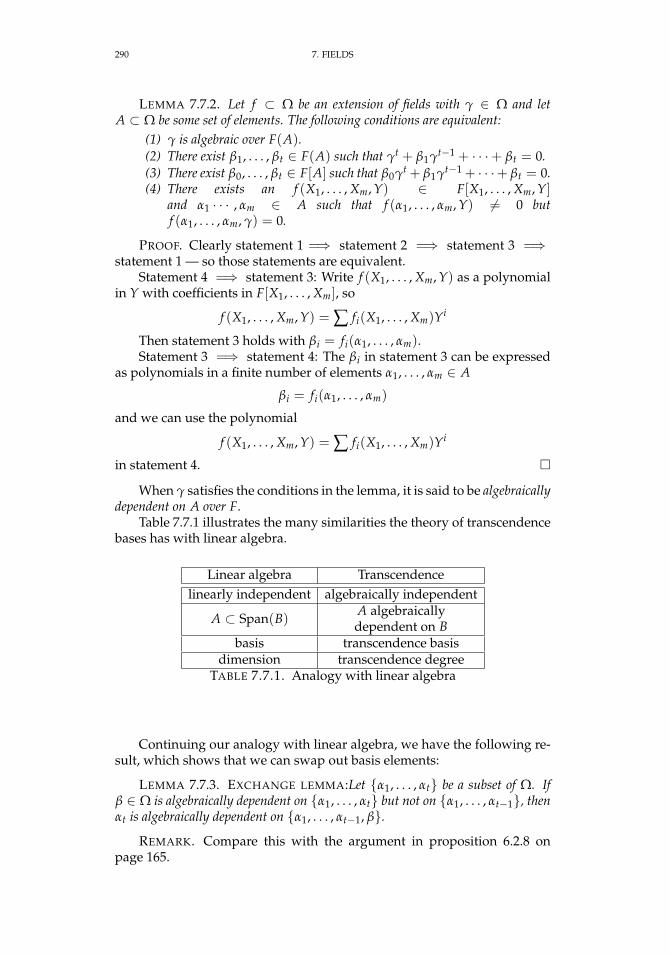
290 7. FIELDS
LEMMA 7.7.2. Let f ⊂ Ω be an extension of fields with γ ∈ Ω and letA ⊂ Ω be some set of elements. The following conditions are equivalent:
(1) γ is algebraic over F(A).(2) There exist β1, . . . , βt ∈ F(A) such that γt + β1γt−1 + · · ·+ βt = 0.(3) There exist β0, . . . , βt ∈ F[A] such that β0γt + β1γt−1 + · · ·+ βt = 0.(4) There exists an f (X1, . . . , Xm, Y) ∈ F[X1, . . . , Xm, Y]
and α1 · · · , αm ∈ A such that f (α1, . . . , αm, Y) 6= 0 butf (α1, . . . , αm, γ) = 0.
PROOF. Clearly statement 1 =⇒ statement 2 =⇒ statement 3 =⇒statement 1 — so those statements are equivalent.
Statement 4 =⇒ statement 3: Write f (X1, . . . , Xm, Y) as a polynomialin Y with coefficients in F[X1, . . . , Xm], so
f (X1, . . . , Xm, Y) = ∑ fi(X1, . . . , Xm)Yi
Then statement 3 holds with βi = fi(α1, . . . , αm).Statement 3 =⇒ statement 4: The βi in statement 3 can be expressed
as polynomials in a finite number of elements α1, . . . , αm ∈ A
βi = fi(α1, . . . , αm)
and we can use the polynomial
f (X1, . . . , Xm, Y) = ∑ fi(X1, . . . , Xm)Yi
in statement 4.
When γ satisfies the conditions in the lemma, it is said to be algebraicallydependent on A over F.
Table 7.7.1 illustrates the many similarities the theory of transcendencebases has with linear algebra.
Linear algebra Transcendencelinearly independent algebraically independent
A ⊂ Span(B) A algebraicallydependent on B
basis transcendence basisdimension transcendence degree
TABLE 7.7.1. Analogy with linear algebra
Continuing our analogy with linear algebra, we have the following re-sult, which shows that we can swap out basis elements:
LEMMA 7.7.3. EXCHANGE LEMMA:Let α1, . . . , αt be a subset of Ω. Ifβ ∈ Ω is algebraically dependent on α1, . . . , αt but not on α1, . . . , αt−1, thenαt is algebraically dependent on α1, . . . , αt−1, β.
REMARK. Compare this with the argument in proposition 6.2.8 onpage 165.
7.7. TRANSCENDENTAL EXTENSIONS 291
PROOF. Since β is algebraically dependent on α1, . . . , αt, there existsa polynomial f (X1, . . . , Xi, Y) with coefficients in F such that
f (α1, . . . , αt, Y) 6= 0 f (α1 . . . , αt, β) = 0
Write f as a polynomial in Xt:
f (X1, . . . , Xt, Y) = ∑ zi(X1, . . . , Xt−1, Y)Xit
Because f (α1, . . . , αt, Y) 6= 0 at least one of the zi, say zi0(α1, . . . , αt−1, Y)is not the zero polynomial.
Because β is not algebraically dependent on α1, . . . , αt−1, it followsthat zi0(α1, . . . , αt−1, β) 6= 0. Therefore f (α1, . . . , αt−1, Xt, β) 6= 0.
But, because f (α1, . . . , αt−1, αt, β) = 0, it follows that αt is algebraicallydependent on α1, . . . , αt−1, β.
LEMMA 7.7.4. If C is algebraically dependent on B and B is algebraicallydependent on A, then C is algebraically dependent on A.
PROOF. If γ is algebraic over a field E that is algebraic over F, then γ isalgebraic over F. Apply this with E = F(A ∪ B) and F = F(A).
Now we are ready to prove the main result
THEOREM 7.7.5. Let F ⊂ Ω be an extension of fields, let A = α1, . . . , αtand B = β1, . . . , βm be two subsets of Ω, and suppose
(1) A is algebraically independent over F.(2) A is algebraically dependent on B over F.
Then t ≤ m.
PROOF. Let ` be the number of elements A and B have in common. Ifthis is t, the conclusion follows, so assume it is < t.
WriteB = α1, . . . , α`, β`+1, . . . , βm
Since α`+1 is algebraically dependent on B, but not on α1, . . . , αt,there will be a β j with ` + 1 ≤ j ≤ m such that α`+1 is algebraically de-pendent on α1, . . . , α`, β`+1, . . . , β j but not on α1, . . . , α`, β`+1, . . . , β j−1.
The Exchange lemma 7.7.3 on the facing page shows that β j is alge-braically dependent on
B1 = B ∪ α`+1 \ β jSo B is algebraically dependent on B1 and A is algebraically dependent onB1. Now we have `+ 1 elements in common between A and B1.
If `+ 1 < t repeat this process, using the Exchange property to swapelements of A for elements of B. We will eventually get ` = t, and t ≤m.
THEOREM 7.7.6. Let F ⊂ Ω be an inclusion of fields. Then there existsa (possibly infinite) set of elements α1, . . . , αk ∈ Ω such that the setα1, . . . , αk is algebraically independent over F, and Ω is an algebraicextension of F(α1, . . . , αk)
The number k is uniquely determined by Ω and is called the transcendencedegree of Ω over F.
292 7. FIELDS
PROOF. All chainsA1 ⊂ A2 ⊂ · · ·
of sets of algebraically independent elements have an upper bound, namelytheir union. Zorn’s lemma ( A.2.12 on page 462) implies that there exists amaximal set of algebraically independent elements. If this set is finite and
α1, . . . , αsand
β1, . . . , βtare two maximal algebraically independent sets, theorem 7.7.5 on the pre-ceding page implies that s ≤ t and t ≤ s so s = t.
EXAMPLE. The Lindemann–Weierstrass theorem (see [43] and[12]) proves that if α1, . . . , αn are algebraic numbers that are linearlyindependent over Q, then Q(eα1 , . . . , eαn) has transcendence degree n overQ.
DEFINITION 7.7.7. A transcendence basis for Ω over F is an algebraicallyindependent set A, such that Ω is algebraic over F(A).
If there is a finite set A ⊂ Ω such that Ω is algebraic over F(A), then Ωhas a finite transcendence basis over F. Furthermore, every transcendencebasis of Ω over F is finite and has the same number of elements.
EXAMPLE 7.7.8. Let p1, . . . , pm be the elementary symmetric polynomi-als in X1, . . . Xm.
CLAIM. The field F(X1, . . . , Xm) is algebraic over F(p1, . . . , pm).
Consider a polynomial f (X1, . . . , Xn) ∈ F(X1, . . . , Xm). Theorem 5.5.18on page 142 shows that the product
∏σ∈Sn
(T − f (Xσ(1), . . . , Xσ(n)))
over all permutations of the variables, is a polynomial with coefficients inF(p1, . . . , pm).
It follows that the set p1, . . . , pm must contain a transcendence basisfor F(X1, . . . , Xm) over F.
Since the size of a transcendence basis is unique, the p1, . . . , pmmustbe a transcendence basis and F(X1, . . . , Xm) must be an algebraic extensionof F(p1, . . . , pm).
Here’s an example from complex analysis:
EXAMPLE 7.7.9. Let Ω be the field of meromorphic functions on a com-pact complex manifold.
The only meromorphic functions on the Riemann sphere are the ratio-nal functions in z. It follows that Ω is a pure transcendental extension of C
of transcendence degree 1.
7.7. TRANSCENDENTAL EXTENSIONS 293
EXERCISES.
1. Use the Lindemann–Weierstrass theorem to prove that π is transcen-dental.
2. Show that the extensionC
Q
has an uncountable degree of transcendence.

CHAPTER 8
Galois Theory
“Galois at seventeen was making discoveries of epochal signifi-cance in the theory of equations, discoveries whose consequencesare not yet exhausted after more than a century. ”
— E. T. Bell.
8.1. Before Galois
Galois Theory involves studying when one can solve polynomial equa-tions
(8.1.1) anXn + an−1Xn−1 + · · ·+ a1X + a0 = 0
via radicals — a term that will be made clear.The first case to be solved was with n = 2
X2 + bX + c = 0
with roots given by the Quadratic Formula — familiar to all students
X =−b±
√b2 − 4a
2
Note that√
b2 − 4a is a radical — a quantity easily computed with algebraicproperties that are easy to understand (i.e., its square is b2 − 4a).
The Quadratic Formula dates to 830 A. D. or, depending on one’s pointof view, millennia earlier1.
The solutions of this problem for n = 3 and n = 4 were some of thegreat mathematical triumphs of the Italian Renaissance. In renaissanceItaly, there were public mathematical contests, “bills of mathematical chal-lenge” (cartelli di matematica disfida). They were public written or oral con-tests modeled after knightly duels, with juries, notaries, and witnesses. Thewinner often received a cash prize, but the real prize was fame and thepromise of paying students.
Like magicians, mathematicians often closely guarded their secretmethods.
In 1539, Niccolò Tartaglia revealed his solution to the cubic equation
X3 + aX2 + bX + c = 0
1Purely geometric solutions were known to the ancient Greeks and, possibly, the ancientEgyptians. The process of completing the square dates to around 830 A. D. in a treatise by AlKhwarizmi.
295
296 8. GALOIS THEORY
to Gerolamo Cardano, a Milanese physician and mathematician — whomhe swore to secrecy. This involved a complex series of transformationsTartaglia detailed in a poem2:
(1) First, substitute X = y− a3 to get
y3 + y(
b− a2
3
)+
2a3
27− ba
3+ c = 0
where the quadratic term has been eliminated. Incidentally, thisis a general operation that kills off the n − 1st term in equationslike 8.1.1 on the preceding page.
(2) Now substitute
y = w− 13w
(b− a2
3
)to get
w3 +1
w3
(a2b2
27− ba4
81− b3
27+
a6
729
)+
2a3
27− ab
3+ c = 0
If we multiply this by w3, we get a quadratic equation in w3 whichwe can solve in the usual way.
(3) Then we take the cube root of w3 and do all the inverse substitutionsto get x. To get all three roots of the original cubic equation, wemust take all three cube roots of w3, namely
w, w ·(−1
2+ i√
32
), w ·
(−1
2− i√
32
)Again, we have a solution involving radicals: square roots and cube roots.
Niccolò Fontana Tartaglia (1499/1500 – 1557) was a mathematician, archi-tect, surveyor, and bookkeeper in the then-Republic of Venice (now part ofItaly). Tartaglia was the first to apply mathematics to computing the tra-jectories of cannonballs, known as ballistics, in his Nova Scientia, “A NewScience.”He had a tragic life. As a child, he was one of the few survivors of themassacre of the population of Brescia by French troops in the War of theLeague of Cambrai. His wounds made speech difficult or impossible forhim, prompting the nickname Tartaglia (“stammerer”).
When Cardano broke his oath of secrecy by publishing the formula inhis book Ars Magna, a decade-long rivalry between him and Tartaglia en-sued. To this day, the method outlined above is called Cardano’s Formula— even though Cardano credited it to Tartaglia in his book.
This solution of the cubic equation is notable because it requires the useof complex numbers — even in cases where the roots are all real (in suchcases, the imaginary parts cancel out at the end).
2Modeled on Dante’s Divine Comedy.
8.1. BEFORE GALOIS 297
Gerolamo Cardano (1501 – 1576) was an Italian mathematician, physician,biologist, physicist, chemist, astrologer, astronomer, philosopher, writer,and gambler. He was one of the most influential mathematicians of theRenaissance. He wrote more than 200 works on science.
The case n = 4 was solved by Lodovico Ferrari in 1540 and publishedin 1545. We present Descartes’s treatment of the solution:
Given a general quartic equation
X4 + aX3 + bX2 + cX + d = 0
we first set X = x− a4 to eliminate the X3-term:
x4 + qx2 + rx + s = 0
Now we write
(8.1.2) x4 + qx2 + rx + s = (x2 + kx + `)(x2 − kx + m)
— this is possible because there is no x3-term in the product.Equating equal powers of x in equation 8.1.2 gives
`+ m− k2 = q
k(m− `) = r`m = s
The first two equations imply that
2m = k2 + q + 2r/k
2` = k2 + q− 2r/k
If we plug these into `m = s, we get
k6 + 2qk4 + (q2 − 4s)k2 − r2 = 0
Since this is cubic in k2, we can use the method for solving cubic equationsand determine k, m, and `. At this point the solution of quadratic equationsgives the four roots of our original problem — all of which are algebraicexpressions involving radicals.
If this solution is written down as an equation, it takes up more thanfive pages.
The reader might wonder what alternatives exist to solving equationsby radicals. There are purely numeric methods for finding the roots of apolynomial to an arbitrary accuracy. The problem is that the roots’ struc-tural algebraic properties are impossible to determine.
Expressions involving radicals are even our preferred way of writingdown irrational algebraic numbers.
Although many mathematicians studied the cases where n ≥ 5, theymade no significant progress. The problem would remain open for morethan 250 years — until Abel, Ruffini, and Galois.
298 8. GALOIS THEORY
8.2. Galois
We will explore the life-work of Évariste Galois, much of which hewrote down days before he died.
Évariste Galois (1811 – 1832) was a French mathematician who, while stillin his teens, was able to determine a necessary and sufficient condition fora polynomial to be solvable by radicals. His work laid the foundations forGalois theory, group theory, and two major branches of abstract algebra.He died at age 20 from wounds suffered in a duel.
Given a field extensionE
FGalois theory studies the group of automorphisms of E that leave F fixed.This group of automorphisms has powerful mathematical properties, clas-sifying all of the subfields of F, for instance.
We begin with a definition
DEFINITION 8.2.1. The Galois group of an extension
E
F
denoted Gal(E/F) is defined by
Gal(E/F) = x ∈ Aut(E)|x( f ) = f , for all f ∈ FEXAMPLE 8.2.2. For instance, consider the extension
C
R
Complex conjugation is known to be a automorphism of C that fixes R thatgenerates the Galois group, so
Gal(C/R) = Z2
In fact, elements of the Galois group of a field-extension can be re-garded as generalizations of complex conjugation.
8.3. Isomorphisms of fields
PROPOSITION 8.3.1. Let g: F1 → F2 be an isomorphism of fields, with in-duced isomorphism of polynomial rings σ: F1[X] → F2[X]. Let f (X) ∈ F1[X] bean irreducible polynomial and f (X) = σ( f (X)) ∈ F2[X]. If α1 is a root of f (X)and α2 is a root of f (X), there exists a unique isomorphism G: F1(α1) → F2(α2)extending g:
F1(α1)G // F2(α2)
F1 g// F2
8.3. ISOMORPHISMS OF FIELDS 299
REMARK. Suppose F1 = F2 = Q and g is the identity map. Since X2− 2is irreducible over Q (see theorem 5.6.8 on page 149) with roots ±
√2, this
result implies that the map
Q(√
2) → Q(√
2)√2 7→ −
√2
defines an isomorphism of fields. It is true that Gal(Q(√
2)/Q) = Z2,generated by this automorphism.
PROOF. The isomorphism σ: F1[X] → F2[X] carries the ideal ( f (X))isomorphically to the ideal ( f (X)) so it induces an isomorphism
F1[X]
( f (X))→ F2[X]
( f (X))
We define G to be the composite
F1(α1)∼=−→ F1[X]
( f (X))→ F2[X]
( f (X))
∼=−→ F2[α2]
This is unique because every element of F1(α1) = F1[α1] is a polynomial inα1 with coefficients in F1. Its coefficients are mapped via g, and its imageunder G is uniquely determined by the way α1 is mapped.
PROPOSITION 8.3.2. Let g: F1 → F2 be an isomorphism of fields, with in-duced isomorphism of polynomial rings g: F1[X]→ F2[X]. Let f (X) ∈ F1[X] be apolynomial and f (X) = g( f (X)) ∈ F2[X]. In addition, let E1 be a splitting fieldfor f (X) and E2be a splitting field for f (X). Then
(1) there exists an isomorphism G: E1 → E2 extending g,(2) if f (X) is separable (see definition 7.2.11 on page 267), there exist
[E1: F1] distinct extensions G.
REMARK. Lemma 7.2.9 on page 267 implies that all polynomials areseparable if F has characteristic zero.
PROOF. We prove these statements by induction on [E1: F1].If [E1: F1] = 1, then f (X) already splits into linear factors in F1[X] and
it follows that f (X) also does, so that E2 = F2.If [E1: F1] > 1, let p(X) be an irreducible factor of f (X) of degree ≥ 2,
and let p(X) = g(p(X)). If α1 is a root of p(X) and α2 is a root of p(X),proposition 8.3.1 on the preceding page implies that there exists an isomor-phism φ: F1(α1) → F2(α2) extending g. Since E1 is also a splitting field forf (X) over F1(α1),
[E1: F] = [E1: F1(α1)] · [F(α1): F]
and [F(α1): F] = deg p(X) ≥ 2, induction implies that there exists an iso-morphism G extending φ.
We prove the second statement by induction too. If [E1: F1] = 1, thenE1 = F1 and there is clearly only one extension of g: G = g. So we assume[E1: F1] > 1. Let p(X) be an irreducible factor of f (X). If deg p(X) =1, then p(X) contributes nothing new to E1 and we may replace f (X) byf (X)/p(X) and continue.
300 8. GALOIS THEORY
If deg p(X) = d > 1, let α be a root of p(X) and let p(X) = g(p(X)) ∈F2[X]. In this case,
[E1: F1] = [E1: F1(α)] · [F1(α): F1]
and proposition 8.3.1 on page 298 implies that there are d distinct isomor-phisms (this is where we use separability of f (X))
β: F1(α)→ F2(α)
extending g, where α is a root of p(X). Since[E1: F1(α)] = [E1: F1]/d < [E1: F1], the induction hypothesisimplies that each of these β’s is covered by [E1: F1]/d distinctisomorphisms G: E1 → E2, giving a total of d · ([E1: F1]/d) = [E1: F1]isomorphisms covering g.
We will compute some splitting fields and Galois groups:
EXAMPLE 8.3.3. If ω = e2πi/3 , we know that ω3 − 1 = 0. The polyno-mial X3 − 1 ∈ Q[X] is not irreducible. It factors as
X3 − 1 = (X− 1)(X2 + X + 1)
and the factor X2 + X + 1 is irreducible over Q (if not, its factors would belinear and imply that the cube roots of 1 are rational) — also see section 7.4.1on page 274. It follows that
Q(ω)
Q
is of degree 2, with Q-basis 1, ω. The identity ω2 + ω + 1 = 0 above,implies that ω2 = −1−ω.
The Galois group is Z2, with a generator that swaps ω with ω2 = ω−1.With respect to the Q-basis given, it is[
1 −10 −1
]Now we consider the polynomial X3 − 2 ∈ Q[X]. Its roots are
21/3, 21/3ω, 21/3ω2 = −21/3 − 21/3ω. Since
ω = (21/3)221/3ω/2
we conclude that its splitting field is Q[ω, 21/3]. The Galois group ofQ[ω, 21/3] over Q is generated by α, given by
ω 7→ −1−ω
−1−ω 7→ ω
21/3 7→ 21/3
8.4. ROOTS OF UNITY 301
and β, given by
ω 7→ ω
21/3 7→ 21/3ω
22/3 7→ −22/3 − 22/3ω
21/3ω 7→ −21/3 − 21/3ω
22/3ω 7→ 22/3
EXERCISES.
1. Suppose F is a field with an extension H = F(α1, . . . , αk) and sup-pose f : H → H is an automorphism such that
a. f (β) = β for all β ∈ Fb. f (αi) = αi for i = 1, . . . , n
Show that f is the identity map. It follows that, if f , g: H → H are twoautomorphisms that fix F and map the αi in the same way, then f = g.
8.4. Roots of Unity
Since we are exploring solutions of polynomials via radicals, we areinterested in extensions of the form F(α1/n). Since we are also interestedin splitting fields, we also need to understand extensions of the form Q(ω)where ω = e2πi/n.
DEFINITION 8.4.1. If ω is an nth root of unity — i.e., if ωn = 1 — thenω is primitive if ωi 6= 1 for all 0 < i < n.
REMARK. For example, e2πi/n ∈ C is a primitive nth root of unity, as ise2πik/n ∈ C for k ∈ Z×n , while e2πi(n/2)/n is not (assuming n is even).
We consider the Galois groups of simple field extensions in two cases:
THEOREM 8.4.2. If F is a field and E = F(ω), with ω a primitive nth root ofunity, then Gal(E/F) is isomorphic to a subgroup of Z×n , hence is finite abelian.
PROOF. Exercise 1 implies that an automorphism
f : E→ E
that fixes F is completely determined by its effect on ω. Let σi(ω) = ωi. Forthis to define an automorphism of 〈ω〉, we must have gcd(i, n) = 1 so thati ∈ Z×n . We define a map
g: Gal(E/F)→ Z×n
302 8. GALOIS THEORY
that sends σi to i ∈ Z×n . This is a homomorphism because
(σi σj)(ω) = σi(ωj) = ωij = σij(ω)
If a field already has roots of unity and we form the splitting field of asimple polynomial, we get
THEOREM 8.4.3. If F contains a primitive nth root of unity, f (X) = Xn −a ∈ F[X], and H is the splitting field of f (X), then there exists an injectivehomomorphism
α: Gal(H/F)→ Zn
REMARK. In both cases, the Galois group is finite abelian — hence adirect sum of suitable cyclic groups.
PROOF. If ω is a primitive nth root of unity and β is a root of f (X), thenall the roots are
β, βω, . . . , βωn−1If σ ∈ Gal(H/F), then σ(β) = βωi, and this defines a map α(σ) = i ∈ Zn.If γ ∈ Gal(H/F), then γ(ω) = ω since ω ∈ F. If γ1(β) = βωi1 andγ2(β) = βωi2 , then
γ1γ2(β) = γ1(βωi2) = βωi1 ωi2 = βωi1+i2
which implies thatα(γ1γ2) = i1 + i2
so that α is a homomorphism. That this is an injection follows from exer-cise 1 on the previous page.
COROLLARY 8.4.4. If p is a prime, F is a field with a primitive pth root ofunity, and f (X) = Xp − a ∈ F[X] has splitting field E, then
Gal(E/F) = 1 or Gal(E/F) = Zp
PROOF. In both cases, theorem 8.4.3 implies that Gal(E/F) ⊂ Zp. Theonly subgroups of Zp are 1 and Zp (see proposition 4.3.2 on page 41).
8.5. Group characters
We will study properties of isomorphisms and automorphisms of fields.
DEFINITION 8.5.1. If G is a group and F is a field, a character from G toF is a homomorphism of groups
σ: G → F×
REMARK. We could have defined c as a homomorphism σ: G → F but,if c(g) = 0 for any g ∈ G, then σ(h) = 0 for all h ∈ G, so σ would not bevery interesting.
This is a group-representation of degree-1 and defines a simple appli-cation of group-representation theory. See chapter 11 on page 383 for moreon this subject.
8.5. GROUP CHARACTERS 303
DEFINITION 8.5.2. A set of characters σ1, . . . , σk: G → F× are said to bedependent if there exist α1, . . . , αk ∈ F not all equal to 0, such that
α1σ1(g) + · · ·+ αkσk(g) = 0
for all g ∈ G. Otherwise, they are said to be independent.
REMARK. Compare this to the notion of linear independence for vec-tors (see 6.2.2 on page 163).
Clearly, if σi = σj for any i 6= j, then the set is dependent because wecan write αj = −αi with all of the other α’s equal to 0. It is quite remarkablethat is the only way a set of characters can be dependent:
PROPOSITION 8.5.3. If G is a group, F is a field and
σ1, . . . , σk
are distinct characters from G to F then they are independent.
REMARK. Two distinct vectors can easily be dependent, but the sameis not true of distinct characters.
PROOF. Clearly, a single character must be independent, since it mustbe nonzero. Suppose we have proved that all sets of < n distinct charactersare independent and we have a dependency relation
α1σ1(g) + · · ·+ αnσn(g) = 0
for all g ∈ G. Note that we can assume that all of the α’s are nonzero sincethe vanishing of any of them would imply a dependency relation of a setof < n distinct characters. Multiplying by α−1
n gives us
(8.5.1) β1σ1(g) + · · ·+ σn(g) = 0
where βi = α−1n · αi. Since σ1 6= σn, there exists an element h ∈ G such that
σ1(h) 6= σn(h). Replace g in equation 8.5.1 by h · g to get
β1σ1(h · g) + · · ·+ σn(h · g) = 0
β1σ1(h)σ1(g) + · · ·+ σn(h)σn(g) = 0
and multiplying by σn(h)−1 gives
(8.5.2) β1σn(h)−1 · σ1(h)σ1(g) + · · ·+ σn(g) = 0
Since σ1(h) 6= σn(h) , it follows that σn(h)−1 · σ1(h) 6= 1 and β1σn(h)−1 ·σ1(h) 6= β1. If we subtract equation 8.5.2 from equation 8.5.1 we get
(β1σn(h)−1 · σ1(h)− β1)σ1(g) + · · ·+ 0 = 0
where we know that β1σn(h)−1 · σ1(h) − β1 6= 0. This is a dependencyrelation with < n terms and a contradiction.
COROLLARY 8.5.4. Every set of distinct automorphisms of a field is indepen-dent.
PROOF. Automorphisms of a field are characters from the multiplica-tive group of the field into it.
304 8. GALOIS THEORY
DEFINITION 8.5.5. If E is a field and G = Aut(E) is the group of auto-morphisms. If H ⊂ G is a subset, define
EH = e ∈ E|h(e) = e for all h ∈ Hcalled the fixed field of H .
REMARK. Note that we require H to fix elements of EH pointwise ratherthan preserving the set EH .
It is not hard to see that EH is a subfield of E. It is also not hard to seethat H1 ⊂ H2 implies that
EH2 ⊂ EH1
Consider the following situation: G = g1, . . . , gn is a set of distinctautomorphisms of a field, E, and EG is the fixed subfield. Now let x ∈E \ EG. Since x is mapped non-trivially by G, and the set G is independent,intuition suggests that
g1(x), . . . , gn(x)will be linearly independent for a suitable x.
This is indeed the case:
LEMMA 8.5.6. If E is a field and G = g1, . . . , gn is a set of distinct auto-morphisms of E, then
[E: EG] ≥ n
PROOF. We prove it by contradiction. Suppose [E: EG] = k < n andlet e1, . . . , ekbe a basis for E over EG. Consider the system of k linearequations over E in n unknowns
g1(e1)x1 + · · ·+ gn(e1)xn = 0...
g1(ek)x1 + · · ·+ gn(ek)xn = 0(8.5.3)
Since k < n, there exists a nonvanishing solution (x1, . . . , xn). For ande ∈ E, we have e = ∑k
i=1 ciei . For i = 1, . . . , k, multiply the ith row ofequation 8.5.3 on page 304 by ci to get
c1g1(e1)x1 + · · ·+ c1gn(e1)xn = 0...
ckg1(ek)x1 + · · ·+ ckgn(ek)xn = 0(8.5.4)
or
g1(c1e1)x1 + · · ·+ gn(c1e1)xn = 0...
g1(ckek)x1 + · · ·+ gn(ckek)xn = 0(8.5.5)
and add up all the rows of the result to get
g1(e)x1 + · · ·+ gn(e)xn = 0
for an arbitrary e ∈ E. This contradicts the independence of the gi.

8.5. GROUP CHARACTERS 305
The alert reader may wonder whether strict inequality can occur, i.e.whether it is possible for [E: EG] > n. The answer is yes for the followingreason:
If g1, g2 ∈ G, then the composite, g1 g2, will also fix EG since each ofthe gi fixes it. If g1 g2 /∈ G, let G′ = G ∪ g1 g2 so that |G′| = n + 1,then
EG = EG′
and the previous result shows that
[E: EG] = [E: EG′ ] ≥ n + 1
It turns out that this is the only way we can have [E: EG] > n:
THEOREM 8.5.7. If E is a field and G = g1, . . . , gn is a set of distinctautomorphisms of E that form a group (i.e. composites and inverses of elements ofG are in G), then
[E: EG] = n
PROOF. It will suffice to show that [E: EG] ≤ n, which we will proveby contradiction. Let e1, . . . , en+1 be linearly independent elements of Eover EG (i.e. linearly independent vectors with coefficients in EG).
Now consider the system of n equations in n + 1 unknowns:
g1(e1)x1 + · · ·+ g1(en+1)xn+1 = 0(8.5.6)...
g1(e1)x1 + · · ·+ g1(en+1)xn+1 = 0
where the xi ∈ EG. Since there are more unknowns than equations, thesystem has nontrivial solutions. Choose a solution with the least numberof nonzero components and re-index the ei so that the nonzero componentscome first. We get a solution like
(x1, . . . , xk, 0, . . . , 0)
where all of the xi are nonzero. We will assume that xk = 1 (multiplyingthe equations by x−1
k , if necessary). We also note that k > 1 since k = 1implies that gi(e1) = 0.
We also conclude that not all of the xi ∈ EG, since the row correspond-ing to 1 ∈ G (which exists since G is a group) would contradict the linearindependence of the ei. Again, by re-indexing the ei, if necessary, assumethat x1 /∈ EG.
It follows that there exists a gα such that gα(x1) 6= x1.If
gi(e1)x1 + · · ·+ gi(ek) = 0is an arbitrary row of the system in 8.5.6, act on it via gα to get
(8.5.7) gα · gi(e1)gα(x1) + · · ·+ gα · gi(ek) = 0
Now note that there exists a β ∈ 1, . . . n, with gα · gi = gβ ∈ G, and thatthere is a βth row of the system in 8.5.6:
gβ(e1)x1 + · · ·+ gβ(ek) = 0
306 8. GALOIS THEORY
If we subtract equation 8.5.7 on the previous page from this (using the factthat gα · gi = gβ, so that gα · gi(ek)− gβ(ek) = 0) we get
gβ(e1)(gα(x1)− x1) + · · ·+ gβ(ek−1)(xk−1 − gα(xk−1)) = 0
Since g1, . . . , gn = gα · g1, . . . , gα · gn, as sets, the result of performingthis construction on all rows of equation 8.5.6 on the preceding page, repro-duces these rows (permuting them) — and the entire system.
It follows that there is a solution of the system 8.5.6 on the previouspage with≤ k− 1 nonzero components, contracting the minimality of k.
In many cases, the fixed fields of groups of automorphisms determinethe automorphisms fixing them:
COROLLARY 8.5.8. If E is a field and G1 and G2 are finite subgroups ofAut(E) with EG1 = EG2 , then G1 = G2.
PROOF. Clearly, G1 = G2 implies that EG1 = EG2 . Conversely, assumeEG1 = EG2 and g ∈ G1. Then g fixes EG2 . If g /∈ G2 then EG2 is fixed by|G2|+ 1 distinct automorphisms, namely element of G2 and g. Lemma 8.5.6on page 304 implies that
[E: EG2 ] ≥ |G2|+ 1
while theorem 8.5.7 on the previous page implies that
[E: EG2 ] = |G2|a contradiction. It follows that any g ∈ G1is also in G2, and symmetryimplies that every element of G2 is also in G1.
8.6. Galois Extensions
We will be concerned with a particularly “well-behaved” class of field-extensions.
DEFINITION 8.6.1. LetE
Fbe an extension of fields with Galois group G (see definition 8.2.1 onpage 298). The definition of Galois group implies that
F ⊂ EG
If F = EG, we will call the field extension a Galois extension or a normalextension.
REMARK. Both terms (Galois and normal) are used equally often, sothe reader should be familiar with both.
It is possible to completely characterize when extensions are Galois:
LEMMA 8.6.2. LetE
Fbe a finite extension of fields. The following conditions are equivalent:
8.6. GALOIS EXTENSIONS 307
(1) If G = Gal(E/F), then F = EG — i.e. the extension is Galois.(2) Every irreducible polynomial in F[X] with a root in E is separable and
has all of its roots in E.(3) E is the splitting field of some separable polynomial in F[X].
REMARK. A polynomial f ∈ F[X] is separable if it factors into distinctlinear factors in the algebraic closure.
PROOF. We prove 1 =⇒ 2. If p(X) ∈ F[X] is irreducible with a rootα ∈ E, let αi = gi(α) ∈ E where gi ∈ G are all the distinct values that resultwhen gi runs over the elements of G. Let
f (X) =n
∏i=1
(X− αi)
The coefficients of f (X) are symmetric functions of the αi(seeequation 5.5.13 on page 142). Since elements of G permute the αi, theyfix the coefficients of f (X) and statement 1, implies that these coefficientsare in F. Since every root of f (X) is also one of p(X), it follows that theyhave nontrivial factors in common. Since p(X) is irreducible, it followsthat p(X)| f (X). This implies that
(1) p(X) is separable (its factors occur once), since f (X) is (by construc-tion)
(2) all roots of p(X) lie in E.Now we show that 2 =⇒ 3. If α ∈ E \ F, let p1(X) be its minimal poly-nomial (see definition 7.1.8 on page 261). This is irreducible, and statement2 implies that all of its roots lie in E. If its roots in E are α1 = α, . . . , αk,let F1 = F[α1, . . . , αk] ⊂ E. If F1 = E, we are done. If not, let β ∈ E \ F1with minimal polynomial p2(X) and continue the argument above. Theprocess terminates in a finite number, t, of steps, and E is the splitting fieldof p1(X) · · · pt(X).
Suppose that E is the splitting field of a separable polynomial f (X) ∈F[X]. The implication 3 =⇒ 1 follows from proposition 8.3.2 on page 299,which implies that the identity map of F has precisely [E: F] extensions toE. These are, of course, the automorphisms of E that fix F, or elements ofG = Gal(E/F).
Now, note that (by theorem 8.5.7 on page 305 and proposition 7.1.6 onpage 261):
[E: F] = |G| = [E: EG] · [EG: F]so that [EG: F] = 1 and EG = F.
Here’s a very simple example:
EXAMPLE 8.6.3. The polynomial X2 − 2 ∈ Q[X] splits into
X2 − 2 = (X−√
2)(X +√
2)
in Q[√
2] = Q(√
2) and the Galois group of the extension
Q(√
2)
Q
308 8. GALOIS THEORY
is Z2, where the nontrivial operation is the map√
2 7→ −√
2
A more subtle example is:
EXAMPLE 8.6.4. Suppose k is a field and consider the symmetric group,Sn, acting on E = k[X1, . . . , Xn] by permuting the Xi. These actions de-fine automorphisms of E and we know that ESn = F (see section 5.5.6 onpage 142) where
F = k[σ1, . . . , σn]
and the σi are the elementary symmetric polynomials on the Xj — see equa-tions 5.5.13 on page 142. On the face of it, we don’t know whether thecorresponding extension of fields of fractions
E
F
is Galois — we don’t know whether Gal(E/F) = Sn. Although it must bea subgroup of some symmetric group, there might, conceivably, exist moreautomorphisms of E over F.
This extension is, indeed, Galois because E is the splitting field of thepolynomial in F[T]:
Tn − σ1Tn−1 + σ2Tn−1 + · · ·+ (−1)nσn =n
∏i=1
(T − Xi)
over F. Since any permutation of the Xi fixes F we conclude thatGal(E/F) = Sn .
COROLLARY 8.6.5. IfE
Fis a Galois extension and F ⊂ B ⊂ E is an intermediate subfield of E, then
E
B
is a Galois extension and Gal(E/B) ⊂ Gal(E/F) is the subgroup of automor-phisms that fix B (pointwise3) as well as F.
REMARK. It is not hard to see that the subgroup, Gal(E/B), uniquelydetermines B, since B = EGal(E/B).
PROOF. The hypothesis implies that there exists a separable polyno-mial f (X) ∈ F[X] such that E is its splitting field. It is not hard to see thatf (X) ∈ B[X] as well, with splitting field E, so lemma 8.6.2 on page 306implies the conclusion. The statement about Galois groups is clear.
3I.e., the automorphisms fix each element of B.
8.6. GALOIS EXTENSIONS 309
COROLLARY 8.6.6. LetE
Fbe a Galois extension. Then there exists a finite number of subfields of E containingF.
PROOF. This is because Gal(E/F) has a finite number of subgroups.
Given two intermediate fields we can define a relation between them:
DEFINITION 8.6.7. Let E be a field with subfields F, B1, and B2 withF ⊂ B1 ∩ B2. If there exists an element g ∈ Gal(E/F) such that g(B1) = B2,we say that B1 and B2 are conjugates.
PROPOSITION 8.6.8. LetE
Fbe a Galois extension with conjugate subfields B1, and B2, and suppose g(B1) =B2 for g ∈ Gal(E/F). Then Gal(E/B2) = Gal(E/B1)
g (see definition 4.4.5 onpage 44).
PROOF. If x ∈ Gal(E/B1), then xg−1 maps B2 to B1 and gxg−1 is an au-tomorphism of E that fixes B2 — i.e., an element of Gal(E/B2). Conversely,a similar argument shows that g−1yg ∈ Gal(E/B1) if y ∈ Gal(E/B2) andthat these operations define a 1-1 correspondence between the two Galoisgroups.
THEOREM 8.6.9. IfE
B
Fis a Galois extension with intermediate field B, the following conditions are equiv-alent:
(1) B is equal to its conjugates (i.e., it has no nontrivial conjugates).(2) If x ∈ Gal(E/F), then x|B ∈ Gal(B/F).(3) The extension
B
Fis Galois.
In all of these cases, restriction defines a surjective homomorphism
Gal(E/F)→ Gal(B/F)
with kernel Gal(E/B) so that
Gal(E/B) C Gal(E/F)
310 8. GALOIS THEORY
and
Gal(B/F) ∼= Gal(E/F)Gal(E/B)
PROOF. 1 =⇒ 2 is clear.Assuming 2, we note that restriction defines a group homomorphism
(8.6.1) f : Gal(E/F)→ Gal(B/F)
Since E is Galois over B, lemma 8.6.2 on page 306 implies that E is the split-ting field of some polynomial in B[X], and proposition 8.3.2 on page 299implies that every automorphism of B extends to one (in fact, to [E: B] ofthem) of E.
This means the homomorphism f in 8.6.1 is surjective. It follows that
BGal(B/F) = BGal(E/F) ⊂ EGal(E/F) = F
The definition of Galois group implies that
F ⊂ BGal(B/F)
always, so we conclude that BGal(B/F) = F and the conclusion follows fromdefinition 8.6.1 on page 306.
Now we show that 3 =⇒ 1. Since B is a Galois extension of F,lemma 8.6.2 on page 306 implies that
B = F(α1, . . . , αn)
where the αi are all the roots of a polynomial, f (X), in F[X]. Ifg ∈ Gal(E/F) and α ∈ B is any root of f (X), we claim that g(α) is also aroot of f (X): if f (X) is
Xn + bn−1Xn−1 + · · ·+ b0
with bi ∈ F, thenαk + bk−1αk−1 + · · ·+ b0 = 0
and, if we apply g to it, we get
g(α)k + bk−1g(α)k−1 + · · ·+ b0 = 0
since g(bi) = bi, so g(α) is a root of f (X). It follows that g permutes the αi(since they are all the roots of f (X)) via a permutation σ ∈ Sn and
g(B) = F(g(α1), . . . , g(αn)) = F(ασ(1), . . . , ασ(n)) = B
As for the final statements,
Gal(E/B) C Gal(E/F)
follows from proposition 8.6.8 on the previous page, which implies thatGal(E/B)g = Gal(E/B) for all g ∈ Gal(E/F).
Restriction induces a surjective map
Gal(E/F)→ Gal(B/F)
and the kernel is precisely the elements that fix B, namely Gal(E/B). Thefinal statement follows from proposition 4.4.8 on page 45.
We will be particularly interested in a certain class of field-extensions:
8.6. GALOIS EXTENSIONS 311
DEFINITION 8.6.10. If m ≥ 2 is an integer, a field extension
E
F
is a pure extension of type m if E = F(α), where αm ∈ F. A tower of extensions
F = E0 ⊂ E1 ⊂ · · · ⊂ Ek
is a radical tower if Ei ⊂ Ei+1 is pure for all i. In this case, Ek is called a radicalextension of F.
EXERCISES.
1. If F ⊂ E is a radical extension, show that there exists a tower of pureextensions
F ⊂ E1 ⊂ · · · ⊂ Ek = Esuch that each extension Ei ⊂ Ei+1 is pure of type pi, where pi is a prime.Hint: Look at the solution to exercise 2 on page 87.
2. IfE
Fis a finite field extension, show that there exists a field extension
G
E
that is the splitting field of a polynomial f (X) ∈ F[X].
3. Suppose we are given an extension
E
F
If B and C are subfields of E, their compositum B ∨ C is the intersectionof all the subfields of E containing B and C. Show that if α1, . . . , αn ∈ E,then
F(α1) ∨ · · · ∨ F(αn) = F(α1, . . . , αn)
4. Show that the splitting field constructed in exercise 2 is given by
K = E1 ∨ · · · ∨ En
where each Ei is isomorphic to E via an isomorphism that fixes F.
5. In exercise 2, ifE
F
312 8. GALOIS THEORY
is a radical extension, then so is
G
F
8.7. Solvability by radicals
In this section, we can give a group-theoretic necessary condition for apolynomial to be solvable by radicals.
DEFINITION 8.7.1. If F is a field, f (X) ∈ F[X] is a polynomial, thenf (X) is said to be solvable by radicals if there exists a radical extension
E
F
such that E contains a splitting field of f (X).
REMARK. This simply means that one can write all of the roots of f (X)as algebraic expressions involving radicals.
LEMMA 8.7.2. Let F be a field of characteristic 0, let f (X) ∈ F[X] be solvableby radicals, and let E be a splitting field of f (X). Then
(1) there is a radical tower
F ⊂ R1 ⊂ · · · ⊂ RN
with E ⊂ RN and RN the splitting field of some polynomial over F, andwith each Ri ⊂ Ri+1 a pure extension of type pi where pi is prime.
(2) If F contains the pthi roots of unity for all i, then the Galois group
Gal(E/F) is solvable.
PROOF. Exercise 2 on the preceding page implies that there is an ex-tension
E ⊂ Swhere S is the splitting field of a polynomial F(X) ∈ F[X], and exercise 5on the previous page implies that
F ⊂ S = RN
is a radical extension. Exercise 1 on the preceding page implies that eachstage of this extension is pure of type pj, where pj is a prime. Since F con-tains the pth
i roots of unity, and exercise 8.4.3 on page 302 implies that eachextension
(8.7.1) Ri ⊂ Ri+1
is the splitting field of a polynomial. Lemma 8.6.2 on page 306 implies thatextension 8.7.1 is Galois.
LetGi = Gal(RN/Ri)
8.7. SOLVABILITY BY RADICALS 313
We get a subnormal series
GN = 1 ⊂ GN−1 ⊂ · · · ⊂ G0
and theorem 8.6.9 on page 309 implies that
Gi/Gi−1
is a cyclic group, so that GN is solvable. Since E ⊂ GN , Gal(E/F) is aquotient of Gal(GN/F) (by theorem 8.6.9 on page 309) hence also solvable(by exercise 5 on page 87).
We can eliminate the hypotheses involving roots of unity:
THEOREM 8.7.3. If F is a field of characteristic 0 and f (X) ∈ F[X] that issolvable by radicals and the splitting field of f is H, then Gal(H/F) is a solvablegroup.
PROOF. The hypothesis implies that
F ⊂ R1 ⊂ · · · ⊂ RN
with each Ri ⊂ Ri+1 a pure extension of type a prime pi and with H ⊂ RN ,and RN is the splitting field of a polynomial g(X) ∈ F[X]. If t is the leastcommon multiple of the pi and ω is a primitive tth root of unity, then RN(ω)is the splitting field of (Xt − 1)g(X).
We get a new tower
(8.7.2) F ⊂ F(ω) ⊂ R1(ω) ⊂ · · · ⊂ RN(ω)
Theorem 8.6.9 on page 309
Gal(RN(ω)/F(ω)) C Gal(RN(ω)/F)
and
Gal(F(ω)/F) ∼= Gal(RN(ω)/F)Gal(RN(ω)/F(ω))
which is an abelian group, by theorem 8.4.2 on page 301.Theorem 8.4.3 on page 302 implies that
Gal(Ri+1(ω)/F)Gal(Ri(ω)/F)
∼= Gal(Ri+1(ω)/Ri(ω))
are cyclic groups for all i. Theorem 8.4.2 on page 301 implies thatGal(F(ω)/F) is finite abelian, hence a direct sum of cyclic groups.
Exercise 2 on page 87 implies that Gal(RN(ω)/F) is solvable. SinceGal(H/F) is a quotient of Gal(RN(ω)/F), it must also be solvable.
Now we consider whether there exists a “formula” for the roots of apolynomial.
Recall the field extension
k(X1, . . . , Xn)
k(σ1, . . . , σn)
314 8. GALOIS THEORY
discussed in Example 8.6.4 on page 308. If this extension is solvable by radi-cals, an expression for the roots of
f (T) = Tn − σ1Tn−1 + σ2Tn−1 + · · ·+ (−1)nσn =n
∏i=1
(T − Xi)
involving radicals of coefficients (i.e., the σi) is a formula for them since onecan plug arbitrary values into the indeterminates.
THEOREM 8.7.4 (Abel-Ruffini). If n ≥ 5, there exists no general formula(involving radicals) for the roots of a polynomial of degree n.
REMARK. This is also known as Abel’s Impossibility Theorem. Ruffinigave an incomplete proof in 1799 and Niels Hendrik Abel proved it in 1824.
PROOF. If such a formula exists, Sn must be a solvable group. If it is,then exercise 5 on page 87 implies that the subgroup
An C Sn
is also solvable. Theorem 4.5.15 on page 55 implies that this is not so.
Niels Henrik Abel (1802 – 1829) was a Norwegian mathematician whomade contributions to a variety of fields. His most famous single resultis the first complete proof of the impossibility of solving the general quinticequation in radicals. This question had been unresolved for 250 years. Healso did research in elliptic functions, discovering Abelian functions.Abel made his discoveries while living in poverty and died at the age of 26.
Paolo Ruffini (1765 – 1822) was an Italian mathematician and philosopher.He is most well-known for his attempts to prove that polynomials of degreefive are not solvable by radicals. He was a professor of mathematics at theUniversity of Modena and a medical doctor who conducted research ontyphus.
Galois Theory carries the Abel-Ruffini Theorem several steps further,as the following example shows
EXAMPLE 8.7.5. The polynomial
(8.7.3) f (X) = X5 − 80X + 5 ∈ Q[X]
is irreducible by Eisenstein’s Criterion (theorem 5.6.8 on page 149) with theprime 5. If H is the splitting field of f (X), we claim that Gal(H/Q) = S5.The plot

8.8. GALOIS’S GREAT THEOREM 315
shows that it has three real roots and a pair of complex conjugate roots, sayα, α, β1, β2, β3. Let τ ∈ Gal(H/Q) be complex conjugation. Since f (X) isof degree 5, we have 5
∣∣ [H: Q] and 5∣∣ |Gal(H/Q)|.
Sylow’s First Theorem ( 4.8.1 on page 81), implies that it has a nontrivialSylow 5-group, which has an element of order 5. The only elements of order5 in S5 are 5-cycles (i1, . . . , i5).
By relabeling elements, if necessary, we can assume(1, 2, 3, 4, 5) ∈ Gal(H/Q) ⊂ S5, and exercise 6 on page 58 implies thatGal(H/Q) = S5.
This is an odd and even disturbing result: not only is there no generalformula for the roots of f (X); one cannot even write down these roots inradical notation (if one magically found out what they were). In other words,no expression of the form
3
√1 +
4√
2 +√
10
however complicated — will equal these roots.This leads to deep questions on how one can do concrete calculations
with algebraic numbers. In general, the most one can say is that
“This number is a root of a certain irreducible polynomial.”This isn’t saying much — for instance, these roots can have wildly differentproperties (three of the roots of equation 8.7.3 on the facing page are real,two are complex).
Radical notation allows one to compute numerical values with arbi-trary accuracy and allows on to deduce algebraic properties of numbers.
8.8. Galois’s Great Theorem
In this section we will prove a converse to theorem 8.7.3 on page 313: ifa polynomial’s splitting field has a solvable Galois group, the polynomialis solvable by radicals.
We first need a result involving the characteristic polynomial of field ele-ments (first mentioned in definition 7.3.2 on page 271.
316 8. GALOIS THEORY
THEOREM 8.8.1. Let
(8.8.1) E
F
be a finite Galois extension with Galois group G = Gal(E/F). If α ∈ E, then
χα(X) = ∏σ∈G
(X− σ(α))
In particularNE/F(α) = ∏
σ∈Gσ(α)
andTE/F(α) = ∑
σ∈Gσ(α)
PROOF. Let p(X) be the minimal polynomial (see definition 7.1.8 onpage 261) of α over F, and let d = [E: F(α)].
Lemma 7.3.5 on page 273 implies that
χα(X) = p(X)d
and lemma 8.6.2 on page 306 implies that all of the roots of p(X) lie in E.Furthermore, proposition 8.3.1 on page 298 implies that G maps a fixed rootof p(X) to all of the others, so we get
p(X) = ∏σi∈G
(X− σi(α))
where the σi ∈ G are the elements that send α to distinct images — there aredeg p(X) of them.
A given σ ∈ G has σ(α) = σi(α) if and only if σ ∈ σi H where H =Gal((E/F(α)), and |H| = d. It follows that
∏σ∈G
(X− σ(α)) =
(∏
σi∈G(X− σi(α))
)d
= p(X)d = χα(X)
The properties of the norm are well-known — see lemma 7.3.3on page 272. In the setting of equation 8.8.1, the norm defines ahomomorphism
NE/F: E× → F×
The following result says something about the kernel of this homo-morphism:
THEOREM 8.8.2 (Hilbert’s Theorem 90). Let
(8.8.2) E
F
8.8. GALOIS’S GREAT THEOREM 317
be a finite Galois extension with Galois group G = Gal(E/F) that is cyclic oforder n with generator σ ∈ G. If α ∈ E×, then NE/F(α) = 1 if and only if thereexists β ∈ E× such that
α = β · σ(β)−1
REMARK. This first appeared in a treatise on algebraic number theoryby David Hilbert (available in English translation in [53]).
See theorem 13.3.3 on page 452 for a cohomological statement of this the-orem.
PROOF. First, we verify that
NE/F(β · σ(β)−1) = NE/F(β) · NE/F(σ(β)−1)
= NE/F(β) · NE/F(σ(β))−1
= NE/F(β) · NE/F(β)−1
= 1
Conversely, suppose NE/F(α) = 1 .Define
δ0 = α
δ1 = ασ(α)
...
δi+1 = ασ(δi)
so thatδn−1 = ασ(α)σ2(α) · · · σn−1(α)
which, by theorem 8.8.1 on the facing page, is equal to NE/F(α) = 1.Since the characters 1, σ, σ2, . . . , σn−1 are independent (see defini-
tion 8.5.2 on page 303 and proposition 8.5.3 on page 303_, there exists γ ∈ Esuch that
β = δ0γ + δ1σ(γ) + · · ·+ δn−2σn−2(γ) + σn−1(γ) 6= 0
since δn−1 = 1. If we act on this via σ, we get
σ(β) = σ(δ0)σ(γ) + · · ·+ σ(δn−2)σn−1(γ) + σn(γ)
= α−1(
δ1σ(γ) + · · ·+ δn−2σn−2(γ) + δn−1σn−1(γ))+ γ
= α−1(
δ1σ(γ) + · · ·+ δn−2σn−2(γ) + δn−1σn−1(γ))+ α−1δ0γ
= α−1β
We apply this to
COROLLARY 8.8.3. IfE
F
318 8. GALOIS THEORY
is a Galois extension of degree p, a prime, and F has a primitive pth root of unity,then E = F(β), where βp ∈ F.
PROOF. If ω is a primitive pth root of unity, ω ∈ F and NE/F(ω) =ωp = 1.
Since Gal(E/F) 6= 1, corollary 8.4.4 on page 302 implies thatGal(E/F) ∼= Zp — let σ be a generator. Then theorem 8.8.2 on page 316implies that there exists β ∈ E such that
ω = β · σ(β)−1
or σ(β) = β ·ω−1. This implies that σ(βp) = βp ·ω−p = βp. It follows thatβp ∈ F. The fact that ω 6= 1 implies that β /∈ F.
Since [E: F] = p, a prime, there are no intermediate fields between Eand F, so E = F(β).
LEMMA 8.8.4. Let E be the splitting field of a polynomial f (X) ∈ F[X], andlet F be an extension of F. If E is the splitting field of f (X) in F then restrictiondefines an injective homomorphism
Gal(E/F)→ Gal(E/F)
PROOF. Let E = F(α1, . . . αk) and E = F((α1, . . . αk). Any automor-phism of E that fixes F also fixes F, and so is determined by its effect on theαi (see exercise 1 on page 301). It follows that the homomorphism
Gal(E/F)→ Gal(E/F)
defined by σ 7→ σ|E is injective.
We come to the main object of this section:
THEOREM 8.8.5 (Galois). Let F be a field of characteristic 0 and let
E
F
be a Galois extension. Then Gal(E/F) is a solvable group if and only if there existsa radical extension R of F with E ⊂ R.
A polynomial f (X) ∈ F[X] has a solvable Galois group if and only if it issolvable by radicals.
PROOF. Theorem 8.7.3 on page 313 gives the “if” part of the statement.Suppose G = Gal(E/F) is solvable. We will proceed by induction on
[E: F]. Since G is solvable, it contains a normal subgroup H C G such that[G: H] = p, a prime (see exercise 1 on page 87).
Since G is a solvable group, H = Gal(E/EH) ⊂ G is a solvable groupand induction implies that there exists a tower of subfields
(8.8.3) EH ⊂ R1 ⊂ · · · ⊂ RN
where each term is pure of type some prime.Consider EH ⊂ E. Since H C G, EH is a Galois extension of F. If we
assume F contains a primitive pth root of unity, then corollary 8.8.3 on thepreceding page implies that F ⊂ EH is pure of type p and we can splice
8.9. THE FUNDAMENTAL THEOREM OF ALGEBRA 319
it onto equation 8.8.3 on the preceding page to get the required tower offield-extensions.
If F does not contain a primitive pth root of unity, let F = F(ω), whereω is a primitive pth root of unity, and let E = E(ω). Note that F ⊂ Eis a Galois extension because, if E is the splitting field of f (X), the E isthe splitting field of f (X)(Xp − 1). It also follows that F ⊂ E is a Galoisextension and lemma 8.8.4 on the facing page implies that
Gal(E/F) ⊂ Gal(E/F)
and is, therefore, a solvable group. Induction implies the existence of atower of pure extensions
(8.8.4) F ⊂ R1 ⊂ · · · ⊂ RN
with E ⊂ E ⊂ RN . Since F ⊂ F = F(ω) is a pure extension, we can splicethis onto equation 8.8.4 to get the required result.
EXERCISES.
1. If G is a finite p-group, show that G is solvable.
8.9. The fundamental theorem of algebra
As an application of Galois theory, we will prove
THEOREM 8.9.1 (Fundamental Theorem of Algebra). If p(X) ∈ C[X] isa nonconstant polynomial, then
p(X) = 0
has a solution in the complex numbers.
REMARK. In other words, the field, C, is algebraically closed. Thisalso implies that the algebraic closure of R is C, and that the only properalgebraic extension of R is C.
This is usually proved using complex analysis. We will need a little bitof analysis
FACT 8.9.2 (Intermediate value property). If f (X) ∈ R[X] and f (x1) <0 and f (x2) > 0, there exists a value x with x ∈ (x1, x2) and f (x) = 0.
COROLLARY 8.9.3. If α ∈ R with α > 0, then α has a square root.
PROOF. Consider the polynomial X2 − α and set x1 = 0 and x2 = α +1.
COROLLARY 8.9.4. If α ∈ C, then α has a square root.
320 8. GALOIS THEORY
PROOF. If x = a + bi, let r =√
a2 + b2 (which exists by corollary 8.9.3on the preceding page) and write
α = reiθ
The required square root is√
r · eiθ/2.
COROLLARY 8.9.5. The field, C, has no extensions of degree 2.
PROOF. If F = C[α] is a degree-2 extension, the minimal polynomial ofα is quadratic, which means its roots exist in C — by corollary 8.9.4 on theprevious page.
LEMMA 8.9.6. Every polynomial f (X) ∈ R[X] of odd degree has a real root.
PROOF. This is a variation on the proof of corollary 8.9.3 on the pre-ceding page. If f (X) = Xn + an−1Xn−1 + · · · + a0, where n is odd, sett = 1 + ∑n−1
i=0 |ai|. We claim that f (t) > 0 and f (−t) < 0. Since |ai| ≤ t− 1for all i, we get
|an−1tn−1 + · · ·+ a0| ≤ (t− 1)(tn−1 + · · ·+ 1)= tn − 1 < tn
It follows that f (t) > 0 because the term tn dominates all the others. Thesame reasoning shows that f (−t) < 0.
COROLLARY 8.9.7. There are no field extensions of R of odd degree > 1.
PROOF. Let R ⊂ E be an extension. If α ∈ E, then the minimal polyno-mial of α must have even degree, by lemma 8.9.6. It follows that [R(α): R]is even which means that [E: R] = [E: R(α)][R(α): R] is also even.
Now we are ready to prove theorem 8.9.1 on the preceding page.We claim that it suffices to prove every polynomial in R[X] has a com-
plex root. If f (X) ∈ C[X], then f (X) · f (X) ∈ R[X], and has complex rootsif and only if f (X) does.
If f (X) ∈ R[X] is irreducible, let E be a splitting field of f (X)(X2 +1) containing C. Then R ⊂ E is a Galois extension (see lemma 8.6.2 onpage 306). Let G = Gal(E/R) and let |G| = 2nm where m is odd.
Theorem 4.8.1 on page 81 implies that G has a subgroup, H, of order2n. Let F = EH be the fixed field.
Corollary 8.6.5 on page 308 implies that [E: F] = 2n with Galois groupH. It follows that [E: R] = [E: F] · [F: R] = 2nm, so that [F: R] = m.
Corollary 8.9.7 implies that m = 1, so that |G| = 2n. Let S ⊂ G be thesubgroup corresponding to Gal(E/C). If 2n > 1, it follows that n ≥ 1 sothat |S| > 1. This is also a 2-group, so it is solvable by exercise 1 on theprevious page. It follows that it has a subgroup, T, of index 2, and ET is anextension of C of degree 2 — which contradicts corollary 8.9.5.
We conclude that E = C.
CHAPTER 9
Division Algebras over R
“The next grand extensions of mathematical physics will, in alllikelihood, be furnished by quaternions.”
— Peter Guthrie Tait, Note on a Quaternion Transformation,1863
9.1. The Cayley-Dickson Construction
Algebras are vector-spaces with a multiplication defined on them. Assuch they are more and less general than rings:
more general in that they may fail to be associative. less general in that they are always vector-spaces over a field.
DEFINITION 9.1.1. An algebra over a field, F, is a vector space, V, overF that is equipped with a form of multiplication:
µ: V ×V → V
that is distributive with respect to addition and subtraction(1) µ(x + y, z) = µ(x, z) + µ(y, z)(2) µ(x, y + z) = µ(x, y) + µ(x, z)
for all x, y, z ∈ V, and is also well-behaved with respect to scalar multiplica-tion: µ(kx, y) = µ(x, ky) = kµ(x, y) for k ∈ F.
An algebra is called a division algebra if it contains an identity element, 1 ∈ V such that µ(1, x) = x =
µ(x, 1) for all x ∈ V. Given any nonzero x, y ∈ V, there exists unique elements q1, q2 ∈
V such that y = µ(q1, x) = µ(x, q2).An involution over an algebra is a homomorphism (with respect to ‘+′)
ι: V → V
with ι2 = 1: V → V.
REMARK. Division algebras have left and right quotients which maydiffer (if they are non-associative). For associative algebras, the conditionof being a division algebra is equivalent to elements having multiplicativeinverses.
There are several inequivalent definitions of division algebras in theliterature: one defines them as algebras without zero-divisors, and anotherdefines them as algebras for which nonzero elements have multiplicativeinverses. If an algebra is finite-dimensional, some of these become equiva-lent — see exercise 5 on the next page.
321
322 9. DIVISION ALGEBRAS OVER R
In this chapter, we will several explore division algebras over R — infact, all of them.
Given an algebra with an involution, the Cayley-Dickson Constructioncreates one of twice the dimension that also has an involution:
DEFINITION 9.1.2 (Cayley-Dickson Construction). Let A be an algebrawith an involution given by ι(x) = x∗ for all x ∈ A. Then we can imposean algebra structure on A⊕ A — all ordered pairs of elements (a, b) witha, b ∈ A with addition defined elementwise — and multiplication definedby
(9.1.1) (a, b)(c, d) = (ac− d∗b, da + bc∗)
This has an involution defined by
(9.1.2) (a, b)∗ = (a∗,−b)
If we apply this construction to the real numbers (as a one-dimensionalalgebra over R) and with the trivial involution (i.e., the identity map), weget a two-dimensional algebra over the real numbers — the complex numbers(see definition 2.1.1 on page 6).
EXERCISES.
1. If A is an algebra over R with involution ∗: A → A, let B = A⊕ Abe the Cayley-Dickson construction on A. Show that
a. if xx∗ ∈ R for all x ∈ A, then yy∗ ∈ R for all y ∈ B, and y has aright inverse, i.e. there exists y−1 such that yy−1 = 1.
b. if x∗x ∈ R for all x ∈ A, then y∗y ∈ R for all y ∈ B, and y has a leftinverse.
c. if xx∗ = x∗x for all x ∈ A, then yy∗ = y∗y for all y ∈ Bd. if xx∗ ≥ 0 ∈ R for all x ∈ A and xx∗ = 0 =⇒ x = 0, then the
same is true for all y ∈ B.
2. Let A be an algebra with an involution, ∗: A → A, over R and B bethe result of the Cayley-Dickson construction on A. Show that, if
(9.1.3) (xy)∗ = y∗x∗
for all x, y ∈ A, then(uv)∗ = v∗u∗
for all u, v ∈ B.
3. How is it possible for an algebra to simultaneously have: multiplicative inverses for all nonzero elements zero-divisors?
4. Show that an algebra with the properties described in exercise 3 can-not be a division algebra.
5. If A is a finite-dimensional algebra over R with no zero-divisors,show that every nonzero element has a multiplicative inverse.
9.2. QUATERNIONS 323
6. If A is an n-dimensional algebra over R, we can represent each ele-ment, x ∈ A, by an n× n matrix mx: Rn → Rn that represents the action ofx by left-multiplication. If A is associative, show that mx·y = mxmy (matrix-product) — so matrices faithfully represent the multiplication on A.
If A is not associative, what is the relationship between mx·y and mxmy?
9.2. Quaternions
For years, Hamilton tried to find an analogue to complex numbers forpoints in three-dimensional space. One can easily add and subtract points inR3— but multiplication and division remained elusive.
In a 1865 letter from Hamilton to his son Archibald, he wrote (see [60]):. . . Every morning in the early part of the above-citedmonth1, on my coming down to breakfast, your (then)little brother William Edwin, and yourself, used to askme: “Well, Papa, can you multiply triplets?” Whereto Iwas always obliged to reply, with a sad shake of the head:“No, I can only add and subtract them.”. . .
The answer came to him in October 16, 1843 while he walked along theRoyal Canal with his wife to a meeting of the Royal Irish Academy: Itdawned on him that he needed to go to four dimensions. He discoveredthe formula
(9.2.1) i2 = j2 = k2 = i · j · k = −1
and — in a famous act of vandalism — carved it into the stone of BroughamBridge as he paused on it. A plaque commemorates this inspiration today.
What he discovered was:
DEFINITION 9.2.1. The quaternions, denoted H, is an algebra over R
whose underlying vector-space is R4. An element is written
x = a + b · i + c · j + d · k ∈ R4
where i, j, k are called the quaternion units, and multiplication is defined bythe identities
(9.2.2) i2 = j2 = k2 = −1
(9.2.3) i · j = k, j · k = i, k · i = j
(9.2.4) u · v = −v · uwhere u, v = i, j, k, the quaternion units. The quantity a ∈ R is called thescalar part of x and b · i + c · j + d · k ∈ R3 is called the imaginary part, or thevector-part.
1October, 1843.
324 9. DIVISION ALGEBRAS OVER R
If a ∈ R and v =
v1v2v3
∈ R3, the vector notation (a, v) represents the
quaternion
a + v = a + v1i + v2 j + v3k ∈H
REMARK. Note that, unlike complex multiplication, quaternion-multiplication is not commutative — as shown in equation 9.2.4 onthe preceding page. It is left as an exercise to the reader to deriveequations 9.2.3 on the previous page and 9.2.4 on the preceding page from
i2 = j2 = k2 = i · j · k = −1
We can formulate quaternion multiplication in terms of the vector form:
PROPOSITION 9.2.2. If a+ v, b+w ∈H are two quaternions in their vectorform, then (see definitions 6.2.62 on page 206 and 6.2.71 on page 209)
(9.2.5) (a + v)(b + w) = ab− v •w + a ·w + b · v + v×w
PROOF. We will prove the claim in the case where a = b = 0. Thegeneral case will follow by the distributive laws: statements 1 and 2 indefinition 9.1.1 on page 321.
(0 + v)(0 + w) = vw1i2 + v2w2 j2 + v3w3k2 + v1w2ij + v1w3ik+ v2w1 ji + v2w3 jk+ v3w1ki + v3w2kj
= −v •w + v1w2k− v1w3 j− v2w1k + v2w3i+ v3w1 j− v3w2i
= −v •w + i(v2w3 − v3w2)
+ j(v3w1 − v1w3) + k(v1w2 − v2w1)
= −v •w + v×w
— see 6.2.71 on page 209.
DEFINITION 9.2.3. Let x = a + b · i + c · j + d · k ∈ H be an element.Define its conjugate, denoted x∗, by
x∗ = a− b · i− c · j− d · k
REMARK. Compare this with complex conjugation.
Conjugation is well-behaved with respect to multiplication:
PROPOSITION 9.2.4. If x, y ∈H, with x = a + b · i + c · j + d · k, then
(1) x · x∗ = x∗x = a2 + b2 + c2 + d2 ∈ R
(2) (x · y)∗ = y∗ · x∗ (note the order-reversal!).
9.2. QUATERNIONS 325
PROOF. If x = a + v, with v =
bcd
∈ R3, then x∗ = a − v and
equation 9.2.5 on the preceding page implies that
x · x∗ = a2 + v • v + av− av + v× v (see proposition 6.2.72 on page 210)
= a2 + ‖v‖2
= a2 + b2 + c2 + d2
If x = a + v, y = b + w, then
(xy)∗ = ab− v •w− a ·w− b · v− v×w
and x∗ = a− v, y = b−w so
y∗x∗ = ab− v •w− b · v− a ·w + w× v= ab− v •w− a ·w− b · v− v×w
DEFINITION 9.2.5. If x ∈ H, then the norm of x, denoted ‖x‖ ∈ R, isdefined by
‖x‖ =√
x · x∗
We immediately have
PROPOSITION 9.2.6. If x, y ∈ H, then ‖x‖ = 0 if and only if x = 0 and‖x · y‖ = ‖x‖ · ‖y‖.
PROOF. The first statement follows immediately from proposition 9.2.4on the facing page. The second follows from
‖x · y‖2 = x · y · (x · y)∗= x · y · y∗ · x∗
= ‖y‖2x · x∗
= ‖y‖2‖x‖2
The discovery of quaternions was regarded as a major breakthroughin the mid 1800’s. Many physical laws, including Maxwell’s equations forelectromagnetic fields were stated in terms of quaternions. This initial en-thusiasm faded when people realized:
(1) most applications do not need the multiplicative structure ofquaternions,
(2) unlike vectors, quaternions are limited to three or four dimen-sions2.
2Depending on one’s point of view.
326 9. DIVISION ALGEBRAS OVER R
The ebbs and flows of history are fascinating and ironic: What Hamiltonand his colleagues regarded as his crowning achievement — quaternions— faded in importance, while his “lesser” discoveries like Hamiltonianenergy-functions turned out to be vital to the development of quantum me-chanics.
In the late 20th century, quaternions found new applications with theadvent of computer graphics: unit quaternions express rotations in R3 moreefficiently than any other known representation. They are widely used incomputer games and virtual reality systems3.
In quantum mechanics, the state of a system is given by a wave func-tion whose values lie in C — see [48]. In Dirac’s relativistic wave-equations,the wave function takes its values in H — see [27] (a reprint of Dirac’s orig-inal book). Those equations apply to electrons and other spin-1/2 particles,and predicted the existence of positrons (or anti-electrons) long before theparticles were observed.
Now we will focus on the relationship between quaternions and rota-tions in R3.
Proposition 9.2.6 on the previous page immediately implies that:
PROPOSITION 9.2.7. The set of quaternions, x ∈ H with ‖x‖ = 1 forms agroup called S3.
REMARK. The quaternion group, Q, defined on page 106, consists of±1,±i,±j,±k ⊂ S3.
Since ‖x‖ = 1, it follows that ‖x‖2 = x · x∗ = 1 so that x−1 = x∗.If x = a + bi + cj + dk, the condition ‖x‖ = 1 implies that
a2 + b2 + c2 + d2 = 1
which is the equation of a 3-dimensional sphere in R4. This is the reasonfor the name S3.
We need another version of the Euler formula:
THEOREM 9.2.8 (Quaternionic Euler Formula). Let u ∈ R3 be a unit-vector and let α ∈ R be a scalar. Then
eα·u = cos α + sin α · uPROOF. By equation 9.2.5 on page 324, (α · u)2 = −α2, since u× u = 0
(see proposition 6.2.72 on page 210) and u • u = 1. It follows that
(α · u)2k = (−1)kα2k
(α · u)2k+1 = (−1)kα2k+1 · uThe conclusion follows by plugging these equations into the power-seriesfor ey — equation 2.1.3 on page 7.
3Most such systems hide the quaternions they use. In the OpenSimulator andSecond Life virtual-reality systems, rotations are explicitly called quaternions (somewhatinaccurately).
9.2. QUATERNIONS 327
Now we will explore the relation between quaternions and rotations inR3. If we think of R3 as the subspace of imaginary quaternions, we runinto trouble:
v · (cos α + sin α · u) = − sin α · v • u + cos α · v + sin α · v× u
which is no longer in R3 since it has a scalar component, namely − sin α · v •u.
We next try conjugating v by eα·u
eα·u · v · e−α·u = cos2 α · v+ sin α cos α (uv− vu)− sin2 αuvu
To simplify this, we note that
(9.2.6) uv− vu = 2u× v
(see equation 9.2.5 on page 324) and
uvu = u (−v • u + v× u)
= − (v • u) u− u • (v× u) + u× (v× u)
= − (v • u) u + v(u · u)− u(u · v) (see exercise 25 on page 212)
= −2 (v • u) u + v
It follows that
eα·u · v · e−α·u = cos2 α · v + 2 sin α cos α · u× v
− sin2 α (−2 (v • u) u + v)
=(
cos2 α− sin2 α)· v + 2 sin α cos α · u× v
+ 2 sin2 α · (v • u) u
= cos(2α) · v + sin(2α) · u× v + (1− cos(2α)) · (v • u) u
= (v • u) u + cos(2α) (v− (v • u)) + sin(2α) · u× v
The last equation is identical to equation 6.2.43 on page 212 so we conclude:The conjugation eα·u · v · e−α·u is the result of rotating v onthe axis defined by u by an angle of 2α.
and we get our result
THEOREM 9.2.9. If v, u ∈ R3 ⊂ H are vectors with ‖u‖ = 1, then theresult of rotating v by an angle θ around the axis defined by u is the conjugationin H
r = e(θ/2)·u · v · e−(θ/2)·u ∈ R3 ⊂H
REMARK. There are several advantages of using quaternions over 3× 3orthogonal matrices (see corollary 6.2.69 on page 208) in computer graphicssystems:
(1) Quaternions have four data-values rather than nine.(2) Multiplying unit quaternions requires fewer operations than mul-
tiplying matrices. Computer graphics systems often require manycomposites of rotations.
328 9. DIVISION ALGEBRAS OVER R
(3) Continuously varying rotations are easy to implement inquaternions:
a(t) + b(t)i + c(t)j + d(t)k‖a(t) + b(t)i + c(t)j + d(t)k‖
These are widely used in computer games, virtual reality systems,and avionic control systems. This is relatively difficult to do withother ways of defining rotations (like orthogonal matrices or ro-tations defined in terms of unit vectors and angles — using equa-tion 6.2.43 on page 212).
(4) Quaternions do not have the gimbal problem — which often hap-pens when one defines rotations in terms of angles. Certain val-ues of these angles cause singularities: For instance, at latitudesof ±90 (the Earth’s north and south poles), all longitudes are thesame. If you vary longitude and latitude continuously, the processlocks up whenever the latitude reaches ±90.
(5) It is easy to correct for round-off errors in working with quater-nions. In performing computations with unit quaternions, round-off errors often give quaternions whose length is not quite 1. Onecan simply divide these by their norms and produce valid rota-tions. The same is not true of orthogonal matrices. Round off errorcan give matrices that are only approximately orthogonal. There isno simple way to find the actual orthogonal matrix “closest” toone of these.
Ferdinand Georg Frobenius (1849 – 1917) was a German mathematician,best known for his contributions to the theory of elliptic functions, differ-ential equations, number theory, and group theory.
Next, we will discuss a remarkable result4:
THEOREM 9.2.10 (Frobenius’s Theorem). The only associative division al-gebras over R are R, C, and H.
REMARK. There are several famous theorems called “Frobenius’s The-orem,” including one in differential topology.
PROOF. Let A be an associative division algebra over R. This is a vec-tor space over R, so suppose its basis is b = v1 = 1, . . . , vn— here 1 ∈ Agenerates a one-dimensional sub-algebra R ⊂ A.
If n = 1, then A = R and we’re done. Consequently, we’ll assumen > 1.
For any d ∈ A \R, let R 〈d〉 denote the two-dimensional vector spaceover R spanned by 1 and d.
CLAIM 9.2.11. R 〈d〉 is the maximal commutative subset of all elementsof A that commute with d. Furthermore, it is isomorphic to C.
4The proof given here is due to Palais in [88]. It is shorter than the original.
9.2. QUATERNIONS 329
PROOF. Let F ⊂ A be the subspace of maximal dimension of elementswhich includes R 〈d〉 and is commutative. If x ∈ A commutes with every-thing in F, then F + R · x is commutative, so must equal F. It follows thatx ∈ F — so everything that commutes with F is in F. If x 6= 0 ∈ F then x−1
commutes with everything in F because xy = yx =⇒ x−1y = yx−1. Itfollows that x−1 ∈ F so that F is a field.
Since [F: R] is finite (it is ≤ n), proposition 7.2.2 on page 264 impliesthat the field-extension R ⊂ F is algebraic. The Fundamental Theorem ofAlgebra ( 8.9.1 on page 319) and example 7.5.8 on page 283 imply that F ∼=C.
Since F is isomorphic to C, we can select an element i ∈ F such thati2 = −1.
It follows that A is also a vector space over C (and that n had to be aneven number), with the action of C on A being given by left-multiplication.If n = 2, A = C and we are done.
If n > 2, regard right-multiplication by i ∈ F as defining a linear trans-formation T: A→ A:
Tx = x · i ∈ ASince T2 = −I, its eigenvalues are ±i with corresponding eigenspaces
A±.(1) If x ∈ A+, then Tx = ix so that ix = xi.(2) If x ∈ A−, then Tx = −ix, so that ix = −xi.(3) A = A+ + A−. This follows from the fact that, for all x ∈ A,
x =12(x− ixi) +
12(x + ixi)
where x− ixi ∈ A+ and x + ixi ∈ A−.(4) A = A+⊕ A−. This follows from the preceding statement and the
fact that: A+ ∩ A− = 0.(5) A+ = C and x, y ∈ A− implies that xy ∈ A+ — because of state-
ment 2 above and
(9.2.7) (xy)i = x(yi) = −x(iy) = −(xi)y = (ix)y = i(xy)
(6) dimC A− = 1. If x ∈ A− is any nonzero element, statement 5implies that multiplication by x defines an isomorphism5 x·: A− →A+, so they must have the same dimension over C. We claim thatx2 ∈ R and x2 < 0. Claim 9.2.11 on the facing page implies thatR 〈x〉 is a field isomorphic to C, so it contains x2. In addition,statement 5 implies that x2 ∈ A+ = C so it is in C ∩R 〈x〉. Sincex /∈ C, C ∩ R 〈x〉 = R. If x2 > 0, it would have square roots±√
x2 ∈ R, and a total of three square roots in the field R 〈x〉,which contradicts corollary 7.2.5 on page 265.
(7) A suitable multiple of x ∈ A−, called j, has the property that j2 =−1. If k = ij, then j and k form a basis for A− and the set
1, i, j, k5Because x has an inverse — since A is a division algebra.
330 9. DIVISION ALGEBRAS OVER R
forms a basis for A over R. It is easy to verify that these satisfy theidentities for the quaternion units of H — so we are done.
EXERCISES.
1. If α, β ∈ R and u1, u2 ∈ R3 ⊂ H, is the equation eα·u1 · eβ·u2 =eα·u1+β·u2 valid?
2. Where did the proof of theorem 9.2.10 on page 328 use the fact thatA was associative?
3. Show that the quaternions are the result of applying the Cayley-Dickson construction (definition 9.1.1 on page 322) to the complex num-bers, where the involution on C is complex-conjugation.
4. Given a unit-quaternion
x = a + b · i + c · j + d · kwith
x−1 = a− b · i− c · j− d · kCompute the orthogonal matrix for the rotation defined by y 7→ xyx−1.Recall that
a2 + b2 + c2 + d2 = 1
5. Show that the quaternionic conjugate can be expressed as an alge-braic equation (in sharp contrast to the complex conjugate):
q∗ = −12(q + i · q · i + j · q · j + k · q · k)
9.3. Octonions and beyond
Hamilton’s success in constructing quaternions inspiredmathematicians to research possibilities of higher-dimension division
algebras over R. Frobenius’s Theorem implies that these cannot possibly beassociative.
In 1843, John T. Graves, a friend of Hamilton’s, discovered aneight-dimensional division algebra over R that he called octaves (now calledoctonions). Cayley independently discovered this algebra and published slightlyearlier — causing many to call them Cayley Numbers.
DEFINITION 9.3.1. The octonions, O, consists of R-linear combinations of the 8octonion units
1 = e0, . . . , e7where multiplication is distributive over addition and octonion units multiply viathe table

9.3. OCTONIONS AND BEYOND 331
e3 e5
e6
e7
e1e4
e2
FIGURE 9.3.1. Fano Diagram
× e1 e2 e3 e4 e5 e6 e7
e1 −1 e4 e7 −e2 e6 −e5 −e3e2 −e4 −1 e5 e1 −e3 e7 −e6e3 −e7 −e5 −1 e6 e2 −e4 e1e4 e2 −e1 −e6 −1 e7 e3 −e5e5 −e6 e3 −e2 −e7 −1 e1 e4e6 e5 −e7 e4 −e3 −e1 −1 e2e7 e3 e6 −e1 e5 −e4 −e2 −1
REMARK. As with quaternions, we have e2i = −1 and eiej = −ejei for i 6= j.
Unlike quaternions
(e3e4)e1 = e5 6= e3(e4e1) = −e5
so the octonions are not associative.
One way to represent this multiplication table in compact form involves theFano Diagram in figure 9.3.1.
Every pair (ei, ej) lies on one of the lines in this diagram (where we regard thecircle in the center as a “line”). The third e-element on the line is the product —with the sign determined by whether one must traverse the line in the direction ofthe arrows (giving a positive result) or in the opposite direction. The lines are alsointerpreted as cycles, with ends wrapping around to the beginnings.
The bottom line of figure 9.3.1 implies that e5e2 = e3, and e5e3 = −e2. In thesecond case, we interpret the end of the line as wrapping around to the beginning— and we must traverse it in a direction opposite to the arrows.
Since octonions are non-associative, we consider “flavors of associativity.”
DEFINITION 9.3.2. An algebra, A, is defined to be
(1) power-associative if any single element generates an associative subalge-bra,
(2) alternative if any pair of elements generate an associative subalgebra.
REMARK. Associative algebras clearly satisfy both of these conditions.Power-associative algebras are ones where expressions like x4 are well-defined
— otherwise, one would have to provide brackets specifying the order of the prod-ucts, like ((xx)(xx)).
332 9. DIVISION ALGEBRAS OVER R
THEOREM 9.3.3 (Artin’s Theorem). An algebra, A, is alternative if and only if
(aa)b = a(ab)(ba)a = b(aa)
for all a, b ∈ A.
PROOF. If A is alternative, the two equations given in the statement will betrue.
Conversely, assume these two equations are true. Since a and b are arbitrary,we conclude that (aa)a = a(aa) and (bb)a = b(ba).
Linearity implies that
(a− b)((a− b)a) = a((a− b)a)− b((a− b)a)
= a(aa)− a(ba)− b(aa) + b(ba)
The hypothesis implies that this is equal to
((a− b)(a− b))a = (aa)a− (ab)a− b(aa) + (bb)a
We compare the two to get
a(aa)− a(ba)− b(aa) + b(ba) = (aa)a− (ab)a− b(aa) + (bb)a
and cancel b(aa) to get
a(aa)− a(ba) + b(ba) = (aa)a− (ab)a + (bb)a
subtract off a(aa) = (aa)a and b(ba) = (bb)a to get
−a(ba) = −(ab)a
so a(ba) = (ab)a. This implies that multiplication of all possible combinations ofa’s and b’s is associative. We conclude that the algebra generated by a and b isassociative.
THEOREM 9.3.4. Let A be an associative algebra with involution ∗: A → A, and letB = A⊕ A be the Cayley-Dickson construction applied to A. If
aa∗ = a∗a and a + a∗
commute with all elements of A, and (ab)∗ = b∗a∗ for all elements a, b ∈ A, then B is analternative algebra.
PROOF. We verify the hypotheses of theorem 9.3.3. If x = (a, b) and y = (c, d),the
xx = (aa− b∗b, ba + ba∗) = (aa− b∗b, b(a + a∗))and
(xx)y = ((aa− b∗b)c− d∗b(a + a∗), daa− db∗b + b(a + a∗)c∗)
= (aac− b∗bc− d∗b(a + a∗), daa− db∗b + b(a + a∗)c∗)(9.3.1)
Sincexy = (ac− d∗b, da + bc∗)
we get
x(xy) = (a(ac− d∗b)− (da + bc∗)∗b, (da + bc∗)a + b(ac− d∗b)∗)
= (a(ac− d∗b)− (cb∗ + a∗d∗)b, (da + bc∗)a + b(c∗a∗ − b∗d))
= (aac− ad∗b− cb∗b− a∗d∗b, daa + bc∗a + bc∗a∗ − bb∗d)
= (aac− (a + a∗)d∗b− cb∗b, daa + bc∗(a + a∗)− bb∗d)(9.3.2)
Now we simply compare the right sides of equations 9.3.1 and 9.3.2, using the factthat bb∗ = b∗b and a + a∗commute with all elements of A to see that they are equal.
9.3. OCTONIONS AND BEYOND 333
Another tedious computation verifies the second condition in theorem 9.3.3 on thepreceding page.
As with quaternions, we define
DEFINITION 9.3.5. If x = a0 + a1e1 + · · ·+ a7e7 ∈ O with the ai ∈ R, then itsconjugate, x∗ is defined by
x∗ = a0 − a1e1 − · · · − a7e7
LEMMA 9.3.6. The result of performing the Cayley-Dickson construction (defini-tion 9.1.2 on page 322) on the quaternions is isomorphic to the octonions. We concludethat O is an alternative algebra.
PROOF. It suffices to prove the first statement for the units, following the cor-respondence
1↔ (1, 0)
e1 ↔ (i, 0)
e7 ↔ (−j, 0)
e3 ↔ (k, 0)
e6 ↔ (0, 1)
e5 ↔ (0,−i)
e2 ↔ (0, j)
e4 ↔ (0,−k)
Then, it is just a matter of checking that the Cayley-Dickson product matches thetable in definition 9.3.1 on page 330.
Exercises 1 on page 322 and 2 on page 322 imply that xx∗ ∈ R for all x ∈ O and(xy)∗ = y∗x∗ for all x, y ∈ O. In addition, the definition of the involution impliesthat x + x∗ ∈ R for all x ∈ O. The conclusion follows from theorem 9.3.4 on thefacing page.
As with the complex numbers and quaternions,
DEFINITION 9.3.7. If x ∈ O, define ‖x‖ =√
xx∗, the norm of x. If ‖x‖ = 0, thenx = 0.
REMARK. Exercise 1 on page 322 implies that xx∗ > 0 for all x 6= 0.
LEMMA 9.3.8. If x, y ∈ O then there exists an associative subalgebra Sx,y ⊂ O withx, y, x∗, y∗ ∈ Sx,y.
PROOF. Write
<(x) =x + x∗
2∈ R
=(x) =x− x∗
2The subalgebra of O generated by =(x) and =(y) is associative because O is alter-native. Define Sx,y to be this subalgebra plus R. Since the elements of R commuteand associate with everything in O, we conclude that Sx,y is associative.
Since <(x) ± =(x), <(y) ± =(y), are in Sx,y, it follows that x, y, x∗, y∗ ∈ Sx,y.
This norm is well-behaved in the sense that:
PROPOSITION 9.3.9. If x, y ∈ O, then ‖x · y‖ = ‖x‖ · ‖y‖.
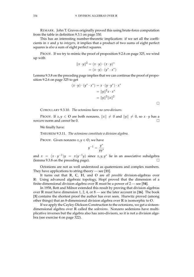
334 9. DIVISION ALGEBRAS OVER R
REMARK. John T. Graves originally proved this using brute-force computationfrom the table in definition 9.3.1 on page 330.
This has an interesting number-theoretic implication: if we set all the coeffi-cients in x and y to integers, it implies that a product of two sums of eight perfectsquares is also a sum of eight perfect squares.
PROOF. If we try to mimic the proof of proposition 9.2.6 on page 325, we windup with
‖x · y‖2 = (x · y) · (x · y)∗
= (x · y) · (y∗ · x∗)Lemma 9.3.8 on the preceding page implies that we can continue the proof of propo-sition 9.2.6 on page 325 to get
(x · y) · (y∗ · x∗) = x · (y · y∗) · x∗
= ‖y‖2x · x∗
= ‖y‖2‖x‖2
COROLLARY 9.3.10. The octonions have no zero-divisors.
PROOF. If x, y ∈ O are both nonzero, ‖x‖ 6= 0 and ‖y‖ 6= 0, so x · y has anonzero norm and cannot be 0.
We finally have:
THEOREM 9.3.11. The octonions constitute a division algebra.
PROOF. Given nonzero x, y ∈ O, we have
y−1 =y∗
yy∗
and x = (x · y−1)y = x(y−1y) since x, y, y∗ lie in an associative subalgebra(lemma 9.3.8 on the preceding page).
Octonions are not as well understood as quaternions and complex numbers.They have applications to string-theory — see [11].
It turns out that R, C, H, and O are all possible division-algebras overR: Using advanced algebraic topology, Hopf proved that the dimension of afinite-dimensional division algebra over R must be a power of 2 — see [54].
In 1958, Bott and Milnor extended this result by proving that division algebrasover R must have dimension 1, 2, 4, or 8 — see the later account in [16]. The book[5] contains the shortest proof the author has ever seen. Hurwitz proved (amongother things) that an 8-dimensional division algebra over R is isomorphic to O.
If we apply the Cayley-Dickson Construction to the octonions, we get a sixteen-dimensional algebra over R called the sedenions. Nonzero sedenions have multi-plicative inverses but the algebra also has zero-divisors, so it is not a division alge-bra (see exercise 4 on page 322).
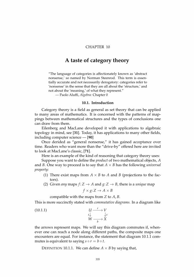
CHAPTER 10
A taste of category theory
“The language of categories is affectionately known as ‘abstractnonsense,’ so named by Norman Steenrod. This term is essen-tially accurate and not necessarily derogatory: categories refer to‘nonsense’ in the sense that they are all about the ‘structure,’ andnot about the ‘meaning,’ of what they represent.”
— Paolo Aluffi, Algebra: Chapter 0
10.1. Introduction
Category theory is a field as general as set theory that can be appliedto many areas of mathematics. It is concerned with the patterns of map-pings between mathematical structures and the types of conclusions onecan draw from them.
Eilenberg and MacLane developed it with applications to algebraictopology in mind, see [31]. Today, it has applications to many other fields,including computer science — [90]
Once derided as “general nonsense,” it has gained acceptance overtime. Readers who want more than the “drive-by” offered here are invitedto look at MacLane’s classic, [71].
Here is an example of the kind of reasoning that category theory uses:Suppose you want to define the product of two mathematical objects, A
and B. One way to proceed is to say that A× B has the following universalproperty:
(1) There exist maps from A × B to A and B (projections to the fac-tors).
(2) Given any maps f : Z → A and g: Z → B, there is a unique map
f × g: Z → A× B
compatible with the maps from Z to A, B.This is more succinctly stated with commutative diagrams. In a diagram like
(10.1.1) U r //
t
Vs
Wb// X
the arrows represent maps. We will say this diagram commutes if, when-ever one can reach a node along different paths, the composite maps oneencounters are equal. For instance, the statement that diagram 10.1.1 com-mutes is equivalent to saying s r = b t.
DEFINITION 10.1.1. We can define A× B by saying that,
335

336 10. A TASTE OF CATEGORY THEORY
(1) it has projection-maps p1: A× B→ A and p2: A× B→ B(2) whenever we have a diagram with solid arrows
(10.1.2) A× B
p1
p2
A Zf
oog//
f×g
OO
B
where Z is an arbitrary “object” that maps to A and B — the dottedof arrow exists, is unique, and makes the whole diagram commute.
In other words, we define A× B by a general structural property thatdoes not use the inner workings or A or B.
DEFINITION 10.1.2. A category, C , is a collection of objects and mor-phisms, which are maps between objects. These must satisfy the conditions:
(1) Given objects x, y ∈ C , homC (x, y) denotes the morphisms fromx to y. This may be an empty set.
(2) Given objects x, y, z ∈ C and morphisms f : x → y and g: y → z,the composition g f : x → z is defined. In other words a dottedarrow exists in the diagram
y
g
x
f
DD
g f// z
making it commute.(3) Given objects x, y, z, w ∈ C and morphisms f : x → y,g: y → z,
h: z → w, composition is associative, i.e., h (g f ) = (h g) f : x → w. This can be represented by a commutative diagram:
x
f
h(g f )=(hg) f//
g f
w
y g//
hg
??
z
h
OO
(4) Every object, x ∈ C , has an identity map 1x: x → x such that, forany f : x → y, f 1x = 1y f = f : x → y. This is equivalent to
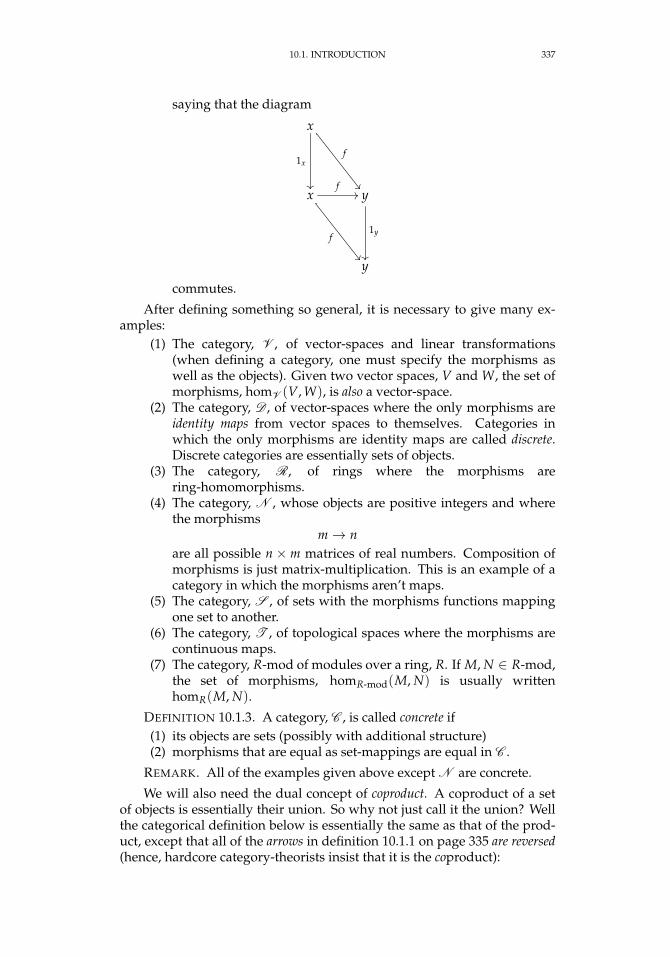
10.1. INTRODUCTION 337
saying that the diagram
x
1x
f
x
f//
f
y
1y
y
commutes.
After defining something so general, it is necessary to give many ex-amples:
(1) The category, V , of vector-spaces and linear transformations(when defining a category, one must specify the morphisms aswell as the objects). Given two vector spaces, V and W, the set ofmorphisms, homV (V, W), is also a vector-space.
(2) The category, D , of vector-spaces where the only morphisms areidentity maps from vector spaces to themselves. Categories inwhich the only morphisms are identity maps are called discrete.Discrete categories are essentially sets of objects.
(3) The category, R, of rings where the morphisms arering-homomorphisms.
(4) The category, N , whose objects are positive integers and wherethe morphisms
m→ nare all possible n × m matrices of real numbers. Composition ofmorphisms is just matrix-multiplication. This is an example of acategory in which the morphisms aren’t maps.
(5) The category, S , of sets with the morphisms functions mappingone set to another.
(6) The category, T , of topological spaces where the morphisms arecontinuous maps.
(7) The category, R-mod of modules over a ring, R. If M, N ∈ R-mod,the set of morphisms, homR-mod(M, N) is usually writtenhomR(M, N).
DEFINITION 10.1.3. A category, C , is called concrete if(1) its objects are sets (possibly with additional structure)(2) morphisms that are equal as set-mappings are equal in C .
REMARK. All of the examples given above except N are concrete.
We will also need the dual concept of coproduct. A coproduct of a setof objects is essentially their union. So why not just call it the union? Wellthe categorical definition below is essentially the same as that of the prod-uct, except that all of the arrows in definition 10.1.1 on page 335 are reversed(hence, hardcore category-theorists insist that it is the coproduct):
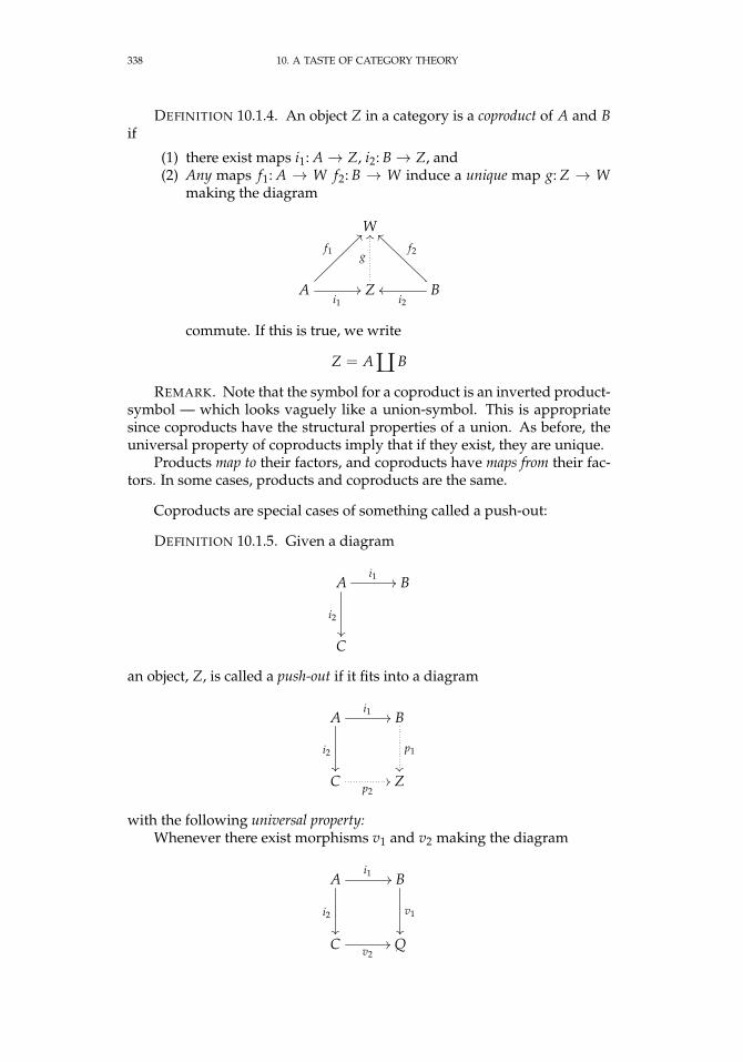
338 10. A TASTE OF CATEGORY THEORY
DEFINITION 10.1.4. An object Z in a category is a coproduct of A and Bif
(1) there exist maps i1: A→ Z, i2: B→ Z, and(2) Any maps f1: A → W f2: B → W induce a unique map g: Z → W
making the diagram
W
A
f1
>>
i1// Z
g
OO
B
f2
__
i2oo
commute. If this is true, we write
Z = A ä B
REMARK. Note that the symbol for a coproduct is an inverted product-symbol — which looks vaguely like a union-symbol. This is appropriatesince coproducts have the structural properties of a union. As before, theuniversal property of coproducts imply that if they exist, they are unique.
Products map to their factors, and coproducts have maps from their fac-tors. In some cases, products and coproducts are the same.
Coproducts are special cases of something called a push-out:
DEFINITION 10.1.5. Given a diagram
Ai1 //
i2
B
C
an object, Z, is called a push-out if it fits into a diagram
Ai1 //
i2
B
p1
C p2// Z
with the following universal property:Whenever there exist morphisms v1 and v2 making the diagram
Ai1 //
i2
B
v1
C v2// Q
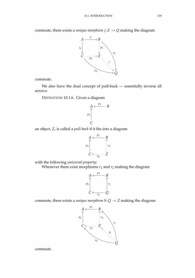
10.1. INTRODUCTION 339
commute, there exists a unique morphism j: Z → Q making the diagram
Ai1 //
i2
B
p1
v1
C p2//
v2 ..
Zj
Q
commute.
We also have the dual concept of pull-back — essentially reverse allarrows:
DEFINITION 10.1.6. Given a diagram
A Bp1
oo
C
p2
OO
an object, Z, is called a pull-back if it fits into a diagram
A Bp1
oo
C
p2
OO
Z
v1
OO
v2oo
with the following universal property:Whenever there exist morphisms r1 and r2 making the diagram
A Bp1
oo
C
p2
OO
Q
r1
OO
r2oo
commute, there exists a unique morphism h: Q→ Z making the diagram
A Bp1
oo
C
p2
OO
Z
v1
OO
v2oo
Q
r1
aa
r2
\\
h
__
commute.
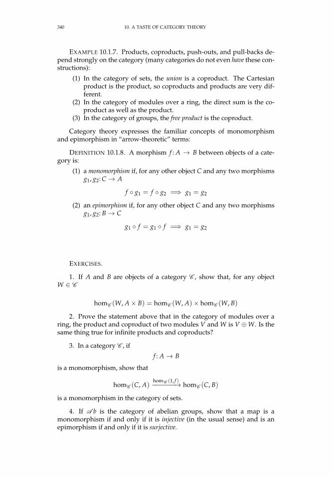
340 10. A TASTE OF CATEGORY THEORY
EXAMPLE 10.1.7. Products, coproducts, push-outs, and pull-backs de-pend strongly on the category (many categories do not even have these con-structions):
(1) In the category of sets, the union is a coproduct. The Cartesianproduct is the product, so coproducts and products are very dif-ferent.
(2) In the category of modules over a ring, the direct sum is the co-product as well as the product.
(3) In the category of groups, the free product is the coproduct.
Category theory expresses the familiar concepts of monomorphismand epimorphism in “arrow-theoretic” terms:
DEFINITION 10.1.8. A morphism f : A → B between objects of a cate-gory is:
(1) a monomorphism if, for any other object C and any two morphismsg1, g2: C → A
f g1 = f g2 =⇒ g1 = g2
(2) an epimorphism if, for any other object C and any two morphismsg1, g2: B→ C
g1 f = g1 f =⇒ g1 = g2
EXERCISES.
1. If A and B are objects of a category C , show that, for any objectW ∈ C
homC (W, A× B) = homC (W, A)× homC (W, B)
2. Prove the statement above that in the category of modules over aring, the product and coproduct of two modules V and W is V ⊕W. Is thesame thing true for infinite products and coproducts?
3. In a category C , if
f : A→ B
is a monomorphism, show that
homC (C, A)homC (1, f )−−−−−−→ homC (C, B)
is a monomorphism in the category of sets.
4. If A b is the category of abelian groups, show that a map is amonomorphism if and only if it is injective (in the usual sense) and is anepimorphism if and only if it is surjective.
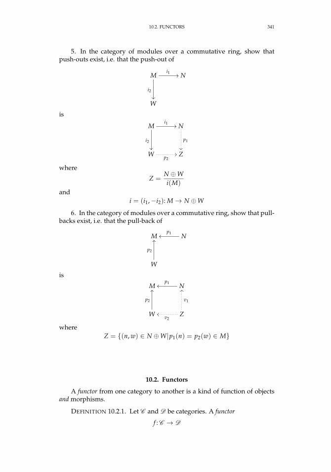
10.2. FUNCTORS 341
5. In the category of modules over a commutative ring, show thatpush-outs exist, i.e. that the push-out of
Mi1 //
i2
N
W
is
Mi1 //
i2
N
p1
W p2// Z
where
Z =N ⊕Wi(M)
andi = (i1,−i2): M→ N ⊕W
6. In the category of modules over a commutative ring, show that pull-backs exist, i.e. that the pull-back of
M Np1
oo
W
p2
OO
is
M Np1
oo
W
p2
OO
Z
v1
OO
v2oo
whereZ = (n, w) ∈ N ⊕W|p1(n) = p2(w) ∈ M
10.2. Functors
A functor from one category to another is a kind of function of objectsand morphisms.
DEFINITION 10.2.1. Let C and D be categories. A functor
f : C → D
342 10. A TASTE OF CATEGORY THEORY
is a function from the objects of C to those of D — i.e., if x ∈ C thenf (x) ∈ D with the following additional property:
If h: x → y is a morphism in C , then f defines, either a morphism f (h): f (x) → f (y) in D — in which case f is called a
covariant functor or just a functor, or a morphism f (h): f (y) → f (x) in D — in which case f is called a
contravariant functor.In addition f (1x) = 1 f (x) and f (j h) = f (j) f (h), if f is covariant orf (j h) = f (h) f (j) is f is contravariant.
REMARK. Functors play an extremely important part in algebraictopology, particularly contravariant ones.
Here are some examples:(1) a functor f : S → S from the category of sets to itself. If x ∈ S ,
f (x) = 2x, the power-set or set of all subsets of x. If d: x → yis a set-mapping and z ⊂ x is a subset, then d|z: z → y is a set-mapping whose images is a subset of y. It follows that d induces anatural map
2d: 2x → 2y
and this is what we define f (d) to be.(2) We can define f : V → V to send a real vector-space, x ∈ V to its
dual, x∗ — the vector-space of all linear transformations η: x → R.If m: x → y is a linear transformation, and µ: y → R is an
element of y∗, the composite η m: x → R is an element of x∗. Weget a natural map m∗: y∗ → x∗ and we set f (m) = m∗. It followsthat f is a contravariant functor.
(3) If F is the category of finite dimensional vector spaces, it is well-known that x∗∗ = x ∈ F , so the functor f defined in statement 2above actually is a contravariant isomorphism of categories
f : F → F
(4) If G is the category of groups and R is that of commutative rings,we can define a functor
gn: R → G
that sends a commutative ring r ∈ R to GLn(r), the group of n× nmatrices whose determinant is a unit of r. Since homomorphismsof rings send units to units, it follows that any homomorphism ofrings
h: r → s
induces a natural homomorphism of groupsgn(h): GLn(r)→ GLn(s).
We can classify functors in various ways:
DEFINITION 10.2.2. A functor f : C → D is:(1) an isomorphism if it is a bijection of objects and morphisms,
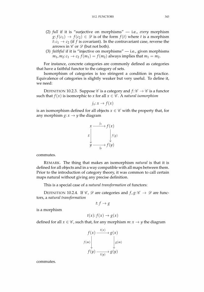
10.2. FUNCTORS 343
(2) full if it is “surjective on morphisms” — i.e., every morphismg: f (c1) → f (c2) ∈ D is of the form f (t) where t is a morphismt: c1 → c2 (if f is covariant). In the contravariant case, reverse thearrows in C or D (but not both).
(3) faithful if it is “injective on morphisms” — i.e., given morphismsm1, m2: c1 → c2 f (m1) = f (m2) always implies that m1 = m2.
For instance, concrete categories are commonly defined as categoriesthat have a faithful functor to the category of sets.
Isomorphism of categories is too stringent a condition in practice.Equivalence of categories is slightly weaker but very useful. To define it,we need:
DEFINITION 10.2.3. Suppose C is a category and f : C → C is a functorsuch that f (x) is isomorphic to x for all x ∈ C . A natural isomorphism
jx: x → f (x)
is an isomorphism defined for all objects x ∈ C with the property that, forany morphism g: x → y the diagram
xjx//
g
f (x)
f (g)
yjy// f (y)
commutes.
REMARK. The thing that makes an isomorphism natural is that it isdefined for all objects and in a way compatible with all maps between them.Prior to the introduction of category theory, it was common to call certainmaps natural without giving any precise definition.
This is a special case of a natural transformation of functors:
DEFINITION 10.2.4. If C , D are categories and f , g: C → D are func-tors, a natural transformation
t: f → g
is a morphismt(x): f (x)→ g(x)
defined for all x ∈ C , such that, for any morphism m: x → y the diagram
f (x)t(x)
//
f (m)
g(x)
g(m)
f (y)t(y)
// g(y)
commutes.
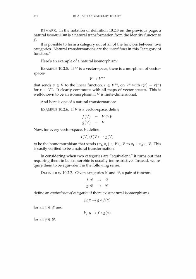
344 10. A TASTE OF CATEGORY THEORY
REMARK. In the notation of definition 10.2.3 on the previous page, anatural isomorphism is a natural transformation from the identity functor tof .
It is possible to form a category out of all of the functors between twocategories. Natural transformations are the morphisms in this “category offunctors.”
Here’s an example of a natural isomorphism:
EXAMPLE 10.2.5. If V is a vector-space, there is a morphism of vector-spaces
V → V∗∗
that sends v ∈ V to the linear function, t ∈ V∗∗, on V∗ with t(r) = r(v)for r ∈ V∗. It clearly commutes with all maps of vector-spaces. This iswell-known to be an isomorphism if V is finite-dimensional.
And here is one of a natural transformation:
EXAMPLE 10.2.6. If V is a vector-space, define
f (V) = V ⊕Vg(V) = V
Now, for every vector-space, V, define
t(V): f (V)→ g(V)
to be the homomorphism that sends (v1, v2) ∈ V ⊕V to v1 + v2 ∈ V. Thisis easily verified to be a natural transformation.
In considering when two categories are “equivalent,” it turns out thatrequiring them to be isomorphic is usually too restrictive. Instead, we re-quire them to be equivalent in the following sense:
DEFINITION 10.2.7. Given categories C and D , a pair of functors
f : C → D
g: D → C
define an equivalence of categories if there exist natural isomorphisms
jx: x → g f (x)
for all x ∈ C andky: y→ f g(x)
for all y ∈ D .
10.3. ADJOINT FUNCTORS 345
EXERCISES.
1. Let f be the functor defined in statement 2 on page 342 above andsuppose we have a morphism
m: V1 → V2
between vector spaces that is represented by a matrix, A. Describe thematrix-representation of
f (m): V∗2 → V∗12. If F is the category of finite-dimensional vector-spaces, show that
the functor f defined in statement 2 on page 342 above is an equivalence ofcategories
f : F → F
Why isn’t it an isomorphism?
3. Find a functor from the category of sets to itself that does not alwayssend injective maps to injective maps.
10.3. Adjoint functors
Adjoint functors are ones that complement each other in a certain sense.They occur naturally in many settings — Daniel Kan was the first to recog-nize these patterns (see [59]) and develop a general concept.
As often happens in category theory, the definition is very cryptic with-out several examples:
DEFINITION 10.3.1. Given two categories, A and B, functors
f : A → B
g: B → A
are said to be adjoint if there exists a natural isomorphism
(10.3.1) homA (x, g(y)) = homB( f (x), y)
for all x ∈ A and y ∈ B. In this situation, f is called a left-adjoint to gand g is called a right-adjoint to f . The collection, ( f , g, A , B) is called anadjunction.
REMARK. Note that (with rare exceptions) f and g are not inverses ofeach other.
Our terminology was taken from Hilbert space theory: U1 and U2 areadjoint operators if
〈U1x, y〉 = 〈x, U2y〉in the Hilbert space, where 〈∗, ∗〉 is the inner product1. Kan was inspired bythis equation’s similarity (in appearance, not function!) to equation 10.3.1on page 345 to name his constructs “adjoints”. Hilbert-space adjoints arenot adjoints in our sense except in certain odd settings (see [10]).
1In finite dimensions, U1 and U2 are matrices, and U2 is the conjugate-transpose of U2.
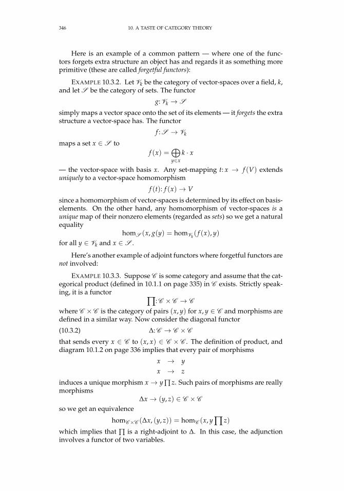
346 10. A TASTE OF CATEGORY THEORY
Here is an example of a common pattern — where one of the func-tors forgets extra structure an object has and regards it as something moreprimitive (these are called forgetful functors):
EXAMPLE 10.3.2. Let Vk be the category of vector-spaces over a field, k,and let S be the category of sets. The functor
g: Vk → S
simply maps a vector space onto the set of its elements — it forgets the extrastructure a vector-space has. The functor
f : S → Vk
maps a set x ∈ S tof (x) =
⊕y∈x
k · x
— the vector-space with basis x. Any set-mapping t: x → f (V) extendsuniquely to a vector-space homomorphism
f (t): f (x)→ V
since a homomorphism of vector-spaces is determined by its effect on basis-elements. On the other hand, any homomorphism of vector-spaces is aunique map of their nonzero elements (regarded as sets) so we get a naturalequality
homS (x, g(y) = homVk( f (x), y)
for all y ∈ Vk and x ∈ S .
Here’s another example of adjoint functors where forgetful functors arenot involved:
EXAMPLE 10.3.3. Suppose C is some category and assume that the cat-egorical product (defined in 10.1.1 on page 335) in C exists. Strictly speak-ing, it is a functor
∏: C × C → C
where C × C is the category of pairs (x, y) for x, y ∈ C and morphisms aredefined in a similar way. Now consider the diagonal functor
(10.3.2) ∆: C → C × C
that sends every x ∈ C to (x, x) ∈ C × C . The definition of product, anddiagram 10.1.2 on page 336 implies that every pair of morphisms
x → yx → z
induces a unique morphism x → y ∏ z. Such pairs of morphisms are reallymorphisms
∆x → (y, z) ∈ C × C
so we get an equivalence
homC×C (∆x, (y, z)) = homC (x, y ∏ z)
which implies that ∏ is a right-adjoint to ∆. In this case, the adjunctioninvolves a functor of two variables.
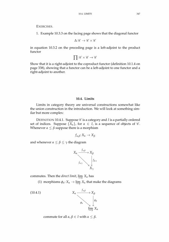
10.4. LIMITS 347
EXERCISES.
1. Example 10.3.3 on the facing page shows that the diagonal functor
∆: C → C × C
in equation 10.3.2 on the preceding page is a left-adjoint to the productfunctor
∏: C × C → C
Show that it is a right-adjoint to the coproduct functor (definition 10.1.4 onpage 338), showing that a functor can be a left-adjoint to one functor and aright-adjoint to another.
10.4. Limits
Limits in category theory are universal constructions somewhat likethe union construction in the introduction. We will look at something sim-ilar but more complex:
DEFINITION 10.4.1. Suppose C is a category and I is a partially orderedset of indices. Suppose Xα, for α ∈ I, is a sequence of objects of C .Whenever α ≤ β suppose there is a morphism
fα,β: Xα → Xβ
and whenever α ≤ β ≤ γ the diagram
Xα
fα,β//
fα,γ
Xβ
fβ,γ
Xγ
commutes. Then the direct limit, lim−→ Xα has
(1) morphisms φα: Xα → lim−→ Xα that make the diagrams
(10.4.1) Xα
fα,β//
φα""
Xβ
φβ
lim−→ Xα
commute for all α, β ∈ I with α ≤ β.
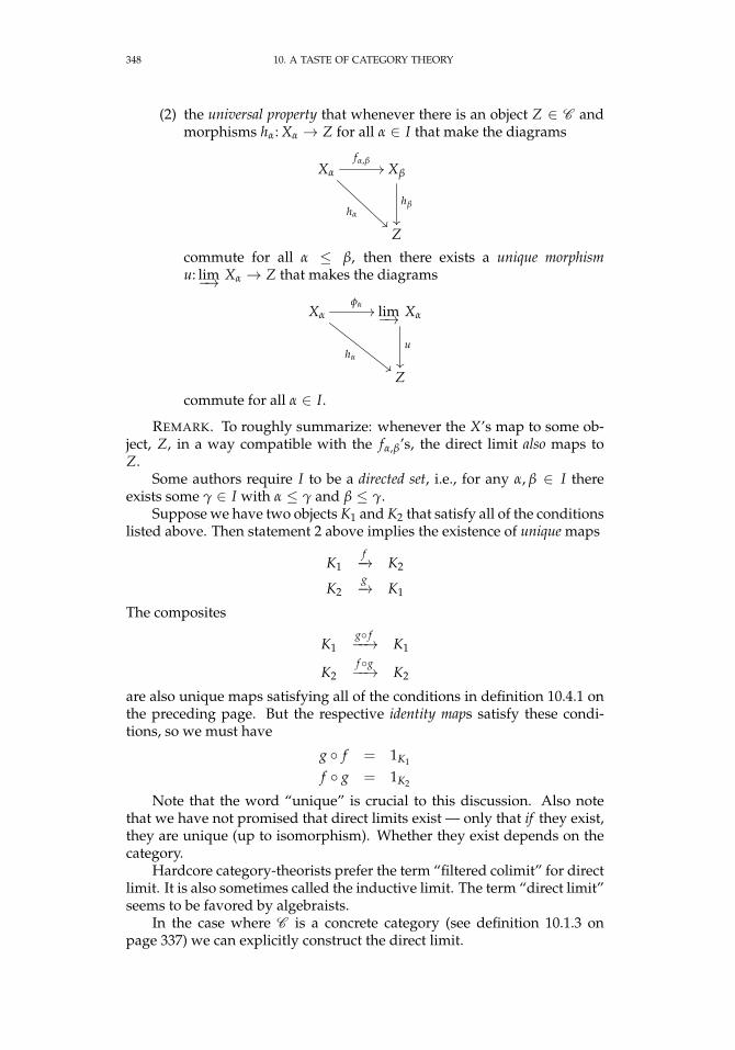
348 10. A TASTE OF CATEGORY THEORY
(2) the universal property that whenever there is an object Z ∈ C andmorphisms hα: Xα → Z for all α ∈ I that make the diagrams
Xα
fα,β//
hα
Xβ
hβ
Z
commute for all α ≤ β, then there exists a unique morphismu: lim−→ Xα → Z that makes the diagrams
Xαφα//
hα
""
lim−→ Xα
u
Z
commute for all α ∈ I.
REMARK. To roughly summarize: whenever the X’s map to some ob-ject, Z, in a way compatible with the fα,β’s, the direct limit also maps toZ.
Some authors require I to be a directed set, i.e., for any α, β ∈ I thereexists some γ ∈ I with α ≤ γ and β ≤ γ.
Suppose we have two objects K1 and K2 that satisfy all of the conditionslisted above. Then statement 2 above implies the existence of unique maps
K1f−→ K2
K2g−→ K1
The composites
K1g f−−→ K1
K2f g−−→ K2
are also unique maps satisfying all of the conditions in definition 10.4.1 onthe preceding page. But the respective identity maps satisfy these condi-tions, so we must have
g f = 1K1
f g = 1K2
Note that the word “unique” is crucial to this discussion. Also notethat we have not promised that direct limits exist — only that if they exist,they are unique (up to isomorphism). Whether they exist depends on thecategory.
Hardcore category-theorists prefer the term “filtered colimit” for directlimit. It is also sometimes called the inductive limit. The term “direct limit”seems to be favored by algebraists.
In the case where C is a concrete category (see definition 10.1.3 onpage 337) we can explicitly construct the direct limit.
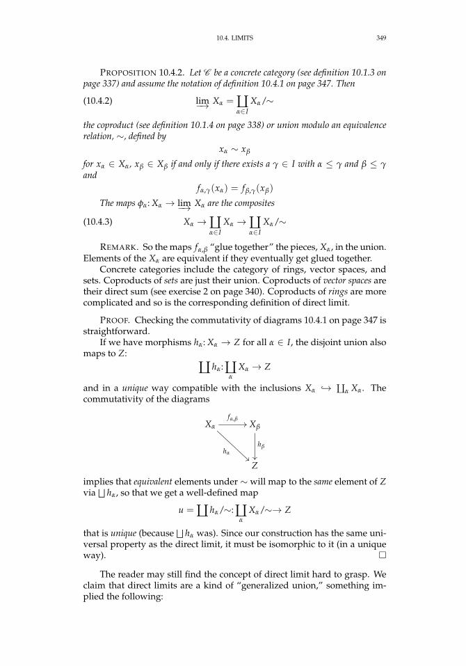
10.4. LIMITS 349
PROPOSITION 10.4.2. Let C be a concrete category (see definition 10.1.3 onpage 337) and assume the notation of definition 10.4.1 on page 347. Then
(10.4.2) lim−→ Xα = äα∈I
Xα/∼
the coproduct (see definition 10.1.4 on page 338) or union modulo an equivalencerelation, ∼, defined by
xα ∼ xβ
for xα ∈ Xα, xβ ∈ Xβ if and only if there exists a γ ∈ I with α ≤ γ and β ≤ γand
fα,γ(xα) = fβ,γ(xβ)
The maps φα: Xα → lim−→ Xα are the composites
(10.4.3) Xα →äα∈I
Xα →äα∈I
Xα/∼
REMARK. So the maps fα,β “glue together” the pieces, Xα, in the union.Elements of the Xα are equivalent if they eventually get glued together.
Concrete categories include the category of rings, vector spaces, andsets. Coproducts of sets are just their union. Coproducts of vector spaces aretheir direct sum (see exercise 2 on page 340). Coproducts of rings are morecomplicated and so is the corresponding definition of direct limit.
PROOF. Checking the commutativity of diagrams 10.4.1 on page 347 isstraightforward.
If we have morphisms hα: Xα → Z for all α ∈ I, the disjoint union alsomaps to Z:
ä hα: äα
Xα → Z
and in a unique way compatible with the inclusions Xα → äα Xα. Thecommutativity of the diagrams
Xα
fα,β//
hα
Xβ
hβ
Z
implies that equivalent elements under ∼ will map to the same element of Zvia
⊔hα, so that we get a well-defined map
u = ä hα/∼: äα
Xα/∼→ Z
that is unique (because⊔
hα was). Since our construction has the same uni-versal property as the direct limit, it must be isomorphic to it (in a uniqueway).
The reader may still find the concept of direct limit hard to grasp. Weclaim that direct limits are a kind of “generalized union,” something im-plied the following:
350 10. A TASTE OF CATEGORY THEORY
PROPOSITION 10.4.3. Assuming the notation of definition 10.4.1 onpage 347 and that C is a concrete category, we have
(10.4.4) lim−→ Xα =⋃α∈I
φα(Xα)
If all of the maps fα,β are injective, then the maps φα: Xα → lim−→ Xα are alsoinjective.
REMARK. If the fα,β are injective, the direct limit is literally a union ofthe Xα.
If they are not injective, and C is a category of groups, rings, or vector-spaces, the direct limit essentially divides out by the kernels of the fα,β —“forcing them” to be injective — and then takes the union.
PROOF. Equation 10.4.4 follows immediately from equations 10.4.2and 10.4.3 on the preceding page.
If all of the fα,β are injective, then the only way two elements x1, x2 ∈Xα can become equivalent is for x1 = x2 ∈ Xα.
EXAMPLE 10.4.4. Suppose I is the set of positive integers and i ≤ j isi|j. Let
Rn = Z
[1n
]Then
fn,m: Rn → Rm
when n|m, is defined to send1n7→ k
mwhere k = m/n. We claim that lim−→ Rn = Q. The maps fn,m are all injectiveand each Rn ⊂ Q so
lim−→ Rn =∞⋃
n=1
Rn ⊂ Q
Since every possible denominator occurs in some Rn this inclusion mustactually be an equality.
DEFINITION 10.4.5. In the notation of definition 10.4.1 on page 347, asubset I′ ⊂ I is said to be cofinal, if for every α ∈ I, there exists a β ∈ I′ suchthat α ≤ β.
REMARK. Cofinal subsets are important because they determine colim-its and limits:
PROPOSITION 10.4.6. In the notation of definition 10.4.1 on page 347, ifI′ ⊂ I is a cofinal subset then
lim−→ Xβ = lim−→ Xα
where α runs over I and β runs over I′.
REMARK. This is significant because direct limits are sometimes easierto compute with cofinal subsets.
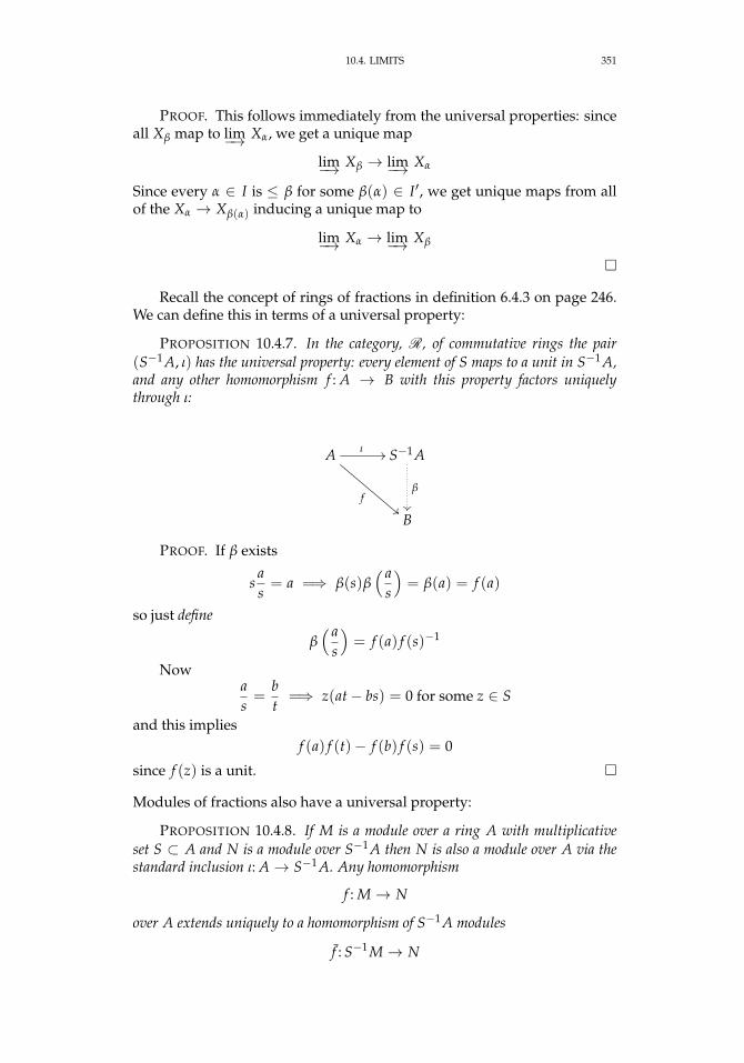
10.4. LIMITS 351
PROOF. This follows immediately from the universal properties: sinceall Xβ map to lim−→ Xα, we get a unique map
lim−→ Xβ → lim−→ Xα
Since every α ∈ I is ≤ β for some β(α) ∈ I′, we get unique maps from allof the Xα → Xβ(α) inducing a unique map to
lim−→ Xα → lim−→ Xβ
Recall the concept of rings of fractions in definition 6.4.3 on page 246.We can define this in terms of a universal property:
PROPOSITION 10.4.7. In the category, R, of commutative rings the pair(S−1 A, ι) has the universal property: every element of S maps to a unit in S−1 A,and any other homomorphism f : A → B with this property factors uniquelythrough ι:
A ι //
f""
S−1 A
β
B
PROOF. If β exists
sas= a =⇒ β(s)β
( as
)= β(a) = f (a)
so just define
β( a
s
)= f (a) f (s)−1
Nowas=
bt
=⇒ z(at− bs) = 0 for some z ∈ S
and this impliesf (a) f (t)− f (b) f (s) = 0
since f (z) is a unit.
Modules of fractions also have a universal property:
PROPOSITION 10.4.8. If M is a module over a ring A with multiplicativeset S ⊂ A and N is a module over S−1 A then N is also a module over A via thestandard inclusion ι: A→ S−1 A. Any homomorphism
f : M→ N
over A extends uniquely to a homomorphism of S−1 A modules
f : S−1M→ N
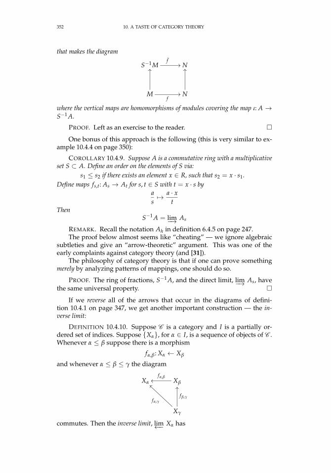
352 10. A TASTE OF CATEGORY THEORY
that makes the diagram
S−1Mf
// N
M
OO
f// N
OO
where the vertical maps are homomorphisms of modules covering the map ι: A →S−1 A.
PROOF. Left as an exercise to the reader.
One bonus of this approach is the following (this is very similar to ex-ample 10.4.4 on page 350):
COROLLARY 10.4.9. Suppose A is a commutative ring with a multiplicativeset S ⊂ A. Define an order on the elements of S via:
s1 ≤ s2 if there exists an element x ∈ R, such that s2 = x · s1.Define maps fs,t: As → At for s, t ∈ S with t = x · s by
as7→ a · x
tThen
S−1 A = lim−→ As
REMARK. Recall the notation Ah in definition 6.4.5 on page 247.The proof below almost seems like “cheating” — we ignore algebraic
subtleties and give an “arrow-theoretic” argument. This was one of theearly complaints against category theory (and [31]).
The philosophy of category theory is that if one can prove somethingmerely by analyzing patterns of mappings, one should do so.
PROOF. The ring of fractions, S−1 A, and the direct limit, lim−→ As, havethe same universal property.
If we reverse all of the arrows that occur in the diagrams of defini-tion 10.4.1 on page 347, we get another important construction — the in-verse limit:
DEFINITION 10.4.10. Suppose C is a category and I is a partially or-dered set of indices. Suppose Xα, for α ∈ I, is a sequence of objects of C .Whenever α ≤ β suppose there is a morphism
fα,β: Xα ← Xβ
and whenever α ≤ β ≤ γ the diagram
Xα Xβ
fα,βoo
Xγ
fβ,γ
OO
fα,γ
``
commutes. Then the inverse limit, lim←− Xα has
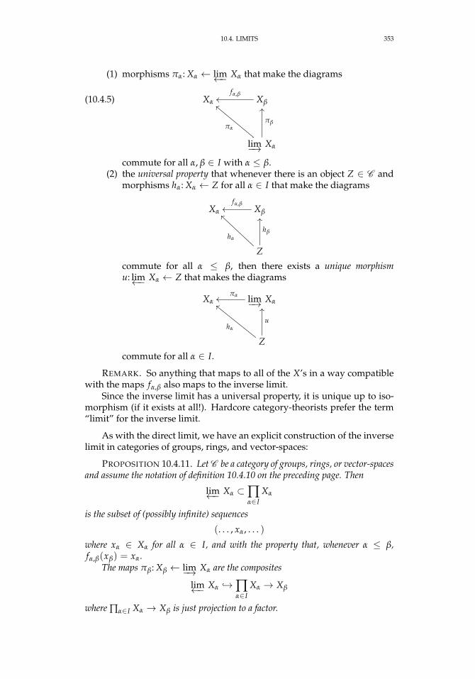
10.4. LIMITS 353
(1) morphisms πα: Xα ← lim←− Xα that make the diagrams
(10.4.5) Xα Xβ
fα,βoo
lim−→ Xα
πβ
OO
πα
bb
commute for all α, β ∈ I with α ≤ β.(2) the universal property that whenever there is an object Z ∈ C and
morphisms hα: Xα ← Z for all α ∈ I that make the diagrams
Xα Xβ
fα,βoo
Z
hβ
OO
hα
``
commute for all α ≤ β, then there exists a unique morphismu: lim←− Xα ← Z that makes the diagrams
Xα lim−→ Xαπαoo
Z
u
OO
hα
bb
commute for all α ∈ I.
REMARK. So anything that maps to all of the X’s in a way compatiblewith the maps fα,β also maps to the inverse limit.
Since the inverse limit has a universal property, it is unique up to iso-morphism (if it exists at all!). Hardcore category-theorists prefer the term“limit” for the inverse limit.
As with the direct limit, we have an explicit construction of the inverselimit in categories of groups, rings, and vector-spaces:
PROPOSITION 10.4.11. Let C be a category of groups, rings, or vector-spacesand assume the notation of definition 10.4.10 on the preceding page. Then
lim←− Xα ⊂∏α∈I
Xα
is the subset of (possibly infinite) sequences
(. . . , xα, . . . )
where xα ∈ Xα for all α ∈ I, and with the property that, whenever α ≤ β,fα,β(xβ) = xα.
The maps πβ: Xβ ← lim−→ Xα are the composites
lim←− Xα →∏α∈I
Xα → Xβ
where ∏α∈I Xα → Xβ is just projection to a factor.
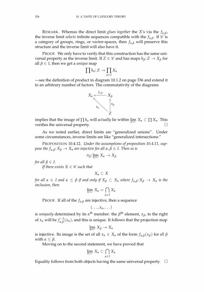
354 10. A TASTE OF CATEGORY THEORY
REMARK. Whereas the direct limit glues together the X’s via the fα,β,the inverse limit selects infinite sequences compatible with the fα,β. If C isa category of groups, rings, or vector-spaces, then fα,β will preserve thisstructure and the inverse limit will also have it.
PROOF. We only have to verify that this construction has the same uni-versal property as the inverse limit. If Z ∈ C and has maps hβ: Z → Xβ forall β ∈ I, then we get a unique map
∏ hα: Z →∏α∈I
Xα
—see the definition of product in diagram 10.1.2 on page 336 and extend itto an arbitrary number of factors. The commutativity of the diagrams
Xα Xβ
fα,βoo
Z
hβ
OO
hα
``
implies that the image of ∏ hα will actually lie within lim←− Xα ⊂ ∏ Xα. Thisverifies the universal property.
As we noted earlier, direct limits are “generalized unions”. Undersome circumstances, inverse limits are like “generalized intersections:”
PROPOSITION 10.4.12. Under the assumptions of proposition 10.4.11, sup-pose the fα,β: Xβ → Xα are injective for all α, β ∈ I. Then so is
πβ: lim←− Xα → Xβ
for all β ∈ I.If there exists X ∈ C such that
Xα ⊂ X
for all α ∈ I and α ≤ β if and only if Xβ ⊂ Xα where fα,β: Xβ → Xα is theinclusion, then
lim←− Xα =⋂α∈I
Xα
PROOF. If all of the fα,β are injective, then a sequence
(. . . , xα, . . . )
is uniquely determined by its αth member: the βth element, xβ, to the rightof xα will be f−1
α,β (xα), and this is unique. It follows that the projection map
lim←− Xβ → Xα
is injective. Its image is the set of all xα ∈ Xα of the form fα,β(xβ) for all βwith α ≤ β.
Moving on to the second statement, we have proved that
lim←− Xα ⊂⋂α∈I
Xα
Equality follows from both objects having the same universal property.

10.4. LIMITS 355
From the proof of proposition 10.4.12 on the preceding page, it is clearthat xβ = f−1
α,β (xα) (if it exists). If fα,β is not injective, all elements of f−1α,β (xα)
give rise to new sequences from the β-position on. For instance:
PROPOSITION 10.4.13. Under the assumptions of proposition 10.4.11, sup-pose that the set of indices, I, is the disjoint union of Ij — i.e. no α ∈ Ij iscomparable with any β ∈ Ik with j 6= k. Then
lim←− Xα︸ ︷︷ ︸α∈I
= ∏j
lim←− Xβ︸ ︷︷ ︸β∈Ij
PROOF. Since the Ij are disjoint they have no influence over each other— all sequences from Ij are paired with all sequences from Ik, j 6= k.
It follows that lim←− Xα can be very large indeed:
EXAMPLE 10.4.14. Let I be positive integers ordered in the usual way,let p ∈ Z be a prime, and let Xn = Zpn for all n. The maps fn,m: Zpm → Zpn
are reduction modulo pn (where n ≤ m).Then
Z(p) = lim←− Xn
is called the p-adic integers and its field of fractions is called the p-adic num-bers, Q(p). Reduction modulo pn (for all n) defines an injection
Z → Z(p)
and, like R, Z(p) is uncountable for all p. These rings were first describedby Hensel in 1897 (see [52]), with a definition wildly different from ours.Hensel showed that one could define infinite series in Q(p) like that for ex
with many number-theoretic applications.Technically, elements of Z(p) are “infinite series”
n0 + n1 · p + n2 · p2 + · · ·such that 0 ≤ ni < p for all i. The image Z ⊂ Z(p) consists of the “series”that terminate after a finite number of terms. Two such “series” are equalif all corresponding ni’s are equal. Define a metric on Z via the p-adicvaluation defined in B.1.3 on page 466
d(m1, m2) =
(12
)vp(m1−m2)
so vp(m1 −m2) is the highest power of p such that
pk|(m1 −m2)
Then Z(p) is the completion of Z in this metric, and two elements, P, Q ofZ(p) are equal if and only if
limi→∞
d(Pi, Qi) = 0
where Pi and Qi are, respectively, the ith partial sums of P and Q.
356 10. A TASTE OF CATEGORY THEORY
Kurt Wilhelm Sebastian Hensel (1861 – 1941) was a German mathematicianborn in Königsberg. He is known for work in number theory, including theintroduction of p-adic numbers.
Here’s another interesting example:
EXAMPLE 10.4.15. Let A be a ring and let m = (X) ⊂ A[X] be an ideal.Then
A[[X]] = lim←− A[X]/mn
On the other hand, if there is a top index in I, the inverse limit is well-behaved:
PROPOSITION 10.4.16. Under the assumptions of proposition 10.4.11 onpage 353, suppose there exists γ ∈ I such that α ≤ γ for all α ∈ I. Then
lim←− Xα = Xγ
PROOF. We could do an algebraic analysis of this statement, but it iseasier to “cheat,” so our proof is: they both have the same universal prop-erty.
EXERCISES.
1. In the category of groups, free groups can be defined using a uni-versal property. What is it?
2. Let C be a category and let C∞ be the category of infinite sequences
· · · → x2 → x1
of morphisms of objects of C . Then
lim←− ∗: C∞ → C
is a functor. Show that this is an adjoint of the functor
∆∞: C → C∞
x 7→ · · · 1−→ x 1−→ x
3. Suppose Xα, for α ∈ I, is a sequence of objects of a concrete cate-gory, C . Whenever α ≤ β suppose there is a morphism
fα,β: Xα → Xβ
and whenever α ≤ β ≤ γ the diagram
Xα
fα,β//
fα,γ
Xβ
fβ,γ
Xγ
commutes. If x, y ∈ Xα map to the same element of lim−→ Xα, show that thereexists a β ≥ α such that fα,β(x) = fα,β(y).

10.5. ABELIAN CATEGORIES 357
4. Show that Prüfer group (see example 4.1.10 on page 38) is given bythe direct limit
Z/p∞ = lim−→ Z/pnZ
where Z/pnZ → Z/pn+1Z multiplies elements by p. Contrast this withexample 10.4.14 on page 355.
10.5. Abelian categories
An abelian category is essentially one in which morphisms of objectshave kernels and cokernels. The standard example is the category of mod-ules over a commutative ring. The official definition is:
DEFINITION 10.5.1. A category A is abelian if:(1) it has products and coproducts of all pairs of objects,(2) it has a zero object (which behaves like an identity for products and
coproducts),(3) all morphisms have a kernel and cokernel:
(a) if Af−→ B is a morphism, there exists a monomorphism K m−→
A such that f m = 0, and if Cg−→ A is any morphism with
f g = 0, there exists a unique morphism v: C → K such that
Cg//
v
A
K
m
OO
commutes.(b) if A
f−→ B is a morphism, there exists an epimorphism B e−→ Esuch that e f = 0, and if g: B → D is any morphism withg f = 0, then there exists a unique morphism v: E→ D suchthat
Bg//
e
D
E
v
OO
(4) the set of morphisms between two objects, homA (A, B), has thestructure of an abelian group for which composition is distributiveover sums.
If F: A → A ′ is a functor between abelian categories, F is said to be additiveif, whenever we have morphisms g1, g2: M→ N in A ,
F(g1 + g2) = F(g1) + F(g2): F(M)→ F(N)
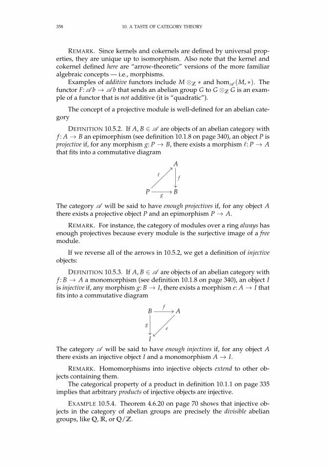
358 10. A TASTE OF CATEGORY THEORY
REMARK. Since kernels and cokernels are defined by universal prop-erties, they are unique up to isomorphism. Also note that the kernel andcokernel defined here are “arrow-theoretic” versions of the more familiaralgebraic concepts — i.e., morphisms.
Examples of additive functors include M ⊗Z ∗ and homA (M, ∗). Thefunctor F: A b → A b that sends an abelian group G to G⊗Z G is an exam-ple of a functor that is not additive (it is “quadratic”).
The concept of a projective module is well-defined for an abelian cate-gory
DEFINITION 10.5.2. If A, B ∈ A are objects of an abelian category withf : A→ B an epimorphism (see definition 10.1.8 on page 340), an object P isprojective if, for any morphism g: P → B, there exists a morphism `: P → Athat fits into a commutative diagram
A
f
P
`
??
g// B
The category A will be said to have enough projectives if, for any object Athere exists a projective object P and an epimorphism P→ A.
REMARK. For instance, the category of modules over a ring always hasenough projectives because every module is the surjective image of a freemodule.
If we reverse all of the arrows in 10.5.2, we get a definition of injectiveobjects:
DEFINITION 10.5.3. If A, B ∈ A are objects of an abelian category withf : B → A a monomorphism (see definition 10.1.8 on page 340), an object Iis injective if, any morphism g: B→ I, there exists a morphism e: A→ I thatfits into a commutative diagram
Bf//
g
A
e
IThe category A will be said to have enough injectives if, for any object Athere exists an injective object I and a monomorphism A→ I.
REMARK. Homomorphisms into injective objects extend to other ob-jects containing them.
The categorical property of a product in definition 10.1.1 on page 335implies that arbitrary products of injective objects are injective.
EXAMPLE 10.5.4. Theorem 4.6.20 on page 70 shows that injective ob-jects in the category of abelian groups are precisely the divisible abeliangroups, like Q, R, or Q/Z.
10.5. ABELIAN CATEGORIES 359
Over the category of modules, we have a criterion for injectivity:
PROPOSITION 10.5.5 (Baer’s Criterion). If R is a commutative ring, an R-module, I is injective if and only if every homomorphism J → I from an idealJ ⊂ R extends to a homomorphism R→ I.
REMARK. In other words, in the category of modules over a ring, in-jectivity only has to be verified for ideals of the ring.
PROOF. The only-if part follows from the definition of injective mod-ules.
Conversely, suppose A ⊂ B are R-modules and f : A → I is a homo-morphism and we consider extensions to submodules B′ with
A ⊂ B′ ⊆ B
These extensions are partially ordered by inclusion. Zorn’s lemma ( A.2.12on page 462) implies that there is a maximal one, B′ say. If B′ 6= B, we willget a contradiction. If b ∈ B \ B′ then J(b) = r ∈ R|r · b ∈ B′ is an ideal
of R and J(b) ·b−→ B′f−→ I defines a homomorphism into I. The hypotheses
imply that this extends to all of R, so b ∈ B′.
Since all abelian groups are modules over Z and all ideals of Z are ofthe form (m) for m ∈ Z, Baer’s Criterion implies that
PROPOSITION 10.5.6. An abelian group, G, is injective if and only if it isdivisible (see definition 4.6.17 on page 69).
Since quotients of divisible groups are divisible (see proposition 4.6.18on page 69), we conclude:
PROPOSITION 10.5.7. Any quotient of an injective object in A b is injectivein A b.
EXAMPLE 10.5.8. In the category of abelian groups, A b, Q and Q/Z
are injective.
This allow us to conclude that the category of abelian groups hasenough injectives (see [8]):
PROPOSITION 10.5.9. If A is an abelian group and
A =FK
where F is a free abelian group, then F⊗Z Q is injective and
A → F⊗Z Q
Kis an injective abelian group containing A so the category of abelian groups, A b,has enough injectives.
It is interesting that this result immediately extends to the category ofmodules over an arbitrary ring (see [30]):
360 10. A TASTE OF CATEGORY THEORY
PROPOSITION 10.5.10. If R is a ring and M is an R-module and I is aninjective abelian group, then
I(R) = homA b(R, I)
is an injective R-module — with R acting on the first factor via
(r′ · ϕ)(r) = ϕ(r′ · r)for ϕ ∈ homA b(R, I). In addition, there exists an injective R-module N and aninclusion
M → N
so that the category of modules over R, MR, has enough injectives.
PROOF. Suppose A ⊂ B is an inclusion of R-modules and g: A →homA b(R, I) is a homomorphism. We will show that this extends to B.Define a natural map
ι: I(R) → If 7→ f (1)
The composite ι g: A → I, regarded as a map of abelian groups, ex-tends to g: B→ I and we define
G: B → homA b(R, I)b 7→ (r 7→ g(r · b))
— a homomorphism of R-modules and the desired extension.To prove the second statement, note the existence of a monomorphism
f : M → homA b(R, M)
m 7→ (r 7→ r ·m)
of R-modules. If we “forget” the module structure of M and regard it onlyas an abelian group, there exists an injective abelian group and a morphism
g: M→ I
The composite
Mf−→ homA b(R, M)
homA b(1,g)−−−−−−−→ homA b(R, I)
is a monomorphism (see exercise 4 on the facing page).
EXERCISES.
1. If M and N are modules over a ring, show that there is a naturalisomorphism
M⊕ N ∼= N ⊕M
2. If A is an abelian group, show that hom(A, Q/Z) = 0 if and only ifA = 0.
10.6. DIRECT SUMS AND TENSOR PRODUCTS 361
3. Show that if we have a monomorphism
f : A→ B
where A is injective, there exists a map
g: B→ A
such that g f = 1: A→ A.
4. If A is an abelian category and
0→ A r−→ B s−→ C → 0
is an exact sequence — i.e., r = ker s and s = coker r, show that
0→ homA (D, A)homA (1,r)−−−−−−→ homA (D, B)
homA (1,s)−−−−−−→ homA (D, C)
is exact.
10.6. Direct sums and Tensor products
The standard example of an abelian category is MR — the category ofmodules over a commutative ring, R.
There are various operations with modules that are most easily under-stood in terms of category theory. The simplest is the direct sum
DEFINITION 10.6.1. If M1, M2 ∈ MR, the direct sum,M1 ⊕M2 ∈ R-mod, is the module of pairs
(m1, m2) ∈ M1 ⊕M2
with R acting viar · (m1, m2) = (r ·m1, r ·m2)
for all r ∈ R, m1 ∈ M1 and m2 ∈ M2.
REMARK. This is just a straightforward generalization of the conceptof direct sum of vector-spaces — and the direct sum is a product and co-product in the category of R-modules.
For instance, the free module Rn is a direct sum
Rn = R⊕ · · · ⊕ R︸ ︷︷ ︸n factors
The direct sum is a functor of two variables:
PROPOSITION 10.6.2. If f1: M1 → N1 and f2: M2 → N2 are morphismsin R-mod, then there is an induced morphism
f1 ⊕ f2: M1 ⊕M2 → N1 ⊕ N2
(m1, m2) 7→ ( f1(m1), f2(m2))
for all m1 ∈ M1 and m2 ∈ M2. In addition, ker( f1 ⊕ f2) = ker f1 ⊕ ker f2.
362 10. A TASTE OF CATEGORY THEORY
PROOF. The only thing that needs to be proved is the statement aboutthe kernels. Clearly ker f1 ⊕ ker f2 ⊂ ker( f1 ⊕ f2). If (m1, m2) maps to 0 inN1 ⊕ N2, we must have f1(m1) = f2(m2) = 0 so this proves ker( f1 ⊕ f2) ⊂ker f1 ⊕ ker f2.
The following concept also originated with linear algebra, but is morecomplex than the direct sum. It is another functor of two variables:
DEFINITION 10.6.3. If M1, M2 ∈ R-mod, then define the tensor productof M1 and M2 over R
M1 ⊗R M2
to be the R-module that is a quotient of the free R-module generated bysymbols m1 ⊗m2 with m1 ∈ M1, m2 ∈ M2 subject to the identities
(1) (r ·m1)⊗m2 = m1⊗ (r ·m2) = r · (m1⊗m2) (defines the R-actionon M1 ⊗R M2) for all r ∈ R, m1 ∈ M1, m2 ∈ M2,
(2) (m1 + m′1)⊗m2 = m1 ⊗m2 + m′1 ⊗m2 for all m1, m′1 ∈ M1, m2 ∈M2,
(3) m1 ⊗ (m2 + m′2) = m1 ⊗m2 + m1 ⊗m′2 for all m1 ∈ M1, m2, m′2 ∈M2.
REMARK. Rule 1 implies that 0⊗ m2 = m1 ⊗ 0 = 0. Here is anotherway to define the tensor product:
Form the free abelian group Z[M1×M2]. Its elements are formal linearcombinations of symbols [m× n] for all m ∈ M1 and n ∈ M2. Then M1 ⊗RM2 = Z[M1×M2]/W, where W ⊂ Z[M1×M2] is the subgroup generatedby
(1) [r ·m1 ×m2]− [m1 × (r ·m2)], [e ·m1 ×m2]− e · [m1 ×m2], for alle ∈ Z, r ∈ R, m1 ∈ M1, and m2 ∈ M2
(2) [(m1 + m′1) × m2] − [m1 × m2] − [m′1 × m2], for all m1, m′1 ∈ M1,m2 ∈ M2,
(3) [m1 × (m2 + m′2)] − [m1 ⊗ m2] − [m1 ⊗ m′2] for all m1 ∈ M1,m2, m′2 ∈ M2.
The R-module structure is defined by setting r · [m1 × m2] = [r · m1 × m2]for all r ∈ R, m1 ∈ M1, m2 ∈ M2
EXAMPLE 10.6.4. If M ∈ R-mod, then
R⊗R M∼=−→ M
r⊗m 7→ r ·mClearly this map is surjective. If r⊗m is in the kernel, then r ·m = 0 ∈ M.In this case, rule 1 in definition 10.6.3 implies that
r · 1⊗m ∼ 1⊗ r ·m = 0
In the category-theoretic sense, M⊗R N is neither a product nor a co-product. It does have a universal property, though:
PROPOSITION 10.6.5. Let M, N, and T be modules over a commutative ring,R, and let
f : M× N → Tbe a mapping with the property that
10.6. DIRECT SUMS AND TENSOR PRODUCTS 363
(1) f |m× N → T is an R-module-homomorphism for any m ∈ M(2) f |M× n→ T is an R-module homomorphism for any n ∈ N(3) f (r ·m, n) = f (m, r · n) for all m ∈ M,n ∈ N, and r ∈ R
Then there exists a unique map
g: M⊗R N → T
that makes the diagram
M× N c //
f''
M⊗R Ng
T
commute, where c(m, n) = m⊗ n, for all m ∈ M and n ∈ N.
REMARK. Here M × N is simply a Cartesian product of sets. A mapsatisfying statements 1 and 2 above is said to be bilinear.
The canonical map
c: M× N → M⊗R N
is not surjective in general since M ⊗R N consists of formal linear combina-tions of symbols m ⊗ n. Elements of M ⊗R N in the image of c are calleddecomposable tensors or elementary tensors. The paper [49] gives criteria forelements of M⊗R N to be decomposable when R is a field.
This result implies that an decomposable tensor m⊗ n vanishes if andonly if every bilinear map
F: M× N → T
sends m× n to 0.
PROOF. The only map Z[M× N]→ T compatible with f is
Z[M× N] → Tm× n 7→ f (m, n)
for all m ∈ M and n ∈ N. The defining relations for M ⊗R N and theconditions on the map f imply that this gives a well-defined map
M⊗ N → Tm⊗ n 7→ f (m, n)
for all m ∈ M and n ∈ N. Since any such map must lift to a map Z[M×N]→ T, this must be unique.
Tensor-products are functors of two variables:
PROPOSITION 10.6.6. Let f : V1 → V2 and g: W1 →W2 be homomorphismsof vector-spaces. Then there is a natural map
f ⊗ g: V1 ⊗k W1 → V2 ⊗k W2
( f ⊗ g)(v⊗ w) = f (v)⊗ g(w)
REMARK. Exercise 5 on page 373 gives some idea of what the homo-morphism f ⊗ g looks like.
364 10. A TASTE OF CATEGORY THEORY
Tensor products are distributive over direct sums, a property that al-lows us to do many computations:
PROPOSITION 10.6.7. Let M, N, T be modules over the commutative ring R.Then there are standard isomorphisms
M⊗R (N ⊕ T) = M⊗R N ⊕M⊗R T
and(M⊕ N)⊗R T = M⊗R T ⊕ N ⊗R T
PROOF. We will prove the first case: the second is similar. We coulduse a detailed algebraic argument, but it is easier to “cheat” and use theuniversal property of a tensor product.
We will show that, given any bilinear map z: M× (N⊕ T)→ Z, whereZ is an R-module, there exists a unique homomorphism d: M⊗R N⊕M⊗RT → Z making the diagram
(10.6.1) M× (N ⊕ T) b //
z**
M⊗R N ⊕M⊗R T
d
Z
commute. Here, b is a bilinear map taking the place of the c map in 10.6.5on page 362. This will show that M⊗R N⊕M⊗R T has the same universalproperty as M⊗R (N ⊕ T) so it must be isomorphic to it.
We begin by constructing a bilinear map b: M× (N⊕ T)→ M⊗R N⊕M⊗R T via b(m, (n, t)) = (m⊗ n, m⊗ t) for all m ∈ M, n ∈ N, and t ∈ T.This is easily verified to be bilinear:
(1) for any fixed m0 ∈ M, `(n, t) = b(m0, (n, t)) = (m0 ⊗ n, m0 ⊗ t)for all n ∈ N and t ∈ T, defines an R-module homomorphism
`: N ⊕ T → M⊗R N ⊕M⊗R T
since the composites
N → m0 ⊗ N ⊂ M⊗R NT → m0 ⊗ T ⊂ M⊗R T
are module-homomorphisms.(2) a similar argument shows that for any fixed n0 ∈ N and t0 ∈ T,
the map `(m) = b(m, (n0, t0)), for all m ∈ M defines a modulehomomorphism
`: M→ M⊗R N ⊕M⊗R T
Now, suppose we have a bilinear map
z: M× (N ⊕ T)→ Z
We will show that there exists a unique map
d: M⊗R N ⊕M⊗R T → Z
that makes diagram 10.6.1 commute.We define d on the direct summands of M⊗R N ⊕M⊗R T:
10.6. DIRECT SUMS AND TENSOR PRODUCTS 365
(1) d1: M⊗R N → Z must send m⊗ n to z(m, (n, 0)) ∈ Z for all m ∈ Mand n ∈ N so we define d1(m⊗ n) = z(m, (n, 0)). The bilinearityof z implies that d1|M⊗ n0: M → Z is a module homomorphismfor any fixed n0 ∈ N and d1|m0 ⊗ N: N → Z is also a modulehomomorphism. It follows that d1 is a module homomorphism.
(2) We define d2: M⊗R T → Z by d2(m⊗ t) = z(m, (0, t)). This is theonly definition compatible with z and an argument like that usedabove shows that it is a module-homomorphism.
We setd = d1 + d2: M⊗R N ⊕M⊗R T → Z
This is a module-homomorphism that makes diagram 10.6.1 on the preced-ing page commute. It is unique because it is uniquely determined on thetwo summands.
COROLLARY 10.6.8. If M ∈ R-mod, R, then
M⊗R Rn = M⊕ · · · ⊕M︸ ︷︷ ︸n times
andRn ⊗R Rm = Rn·m
PROOF. This follows from example 10.6.4 on page 362,proposition 10.6.7 on the preceding page and induction on n.
If R is an algebra over another ring S, we can define the structure of anR-module on A⊗S B by f · (a⊗ b) = (r · a⊗ r · b), for r ∈ R. We can alsodefine an R-action on groups of homomorphisms:
DEFINITION 10.6.9. If M and N are R-modules, where R is anS-algebra, then
HomR(M, N)
denotes morphisms that are R-linear (i.e. morphisms of R-mod) and
HomS(M, N)
are morphisms of S-mod, i.e. morphisms that are S-linear. Then we canequip HomS(M, N) with the structure of an R-module via the rule
If f ∈ HomS(M, N) is such that f (m) = n, then(r · f )(m) = f (r ·m).
We have important relations between homS and homR:
PROPOSITION 10.6.10. If A, B, C ∈ R-mod, where R is an S-algebra, thenthere exists a unique isomorphism
s: HomR(A, HomS(B, C))→ HomR(A⊗S B, C)
REMARK. This is clearly natural with respect to all homomorphisms ofA, B, or C.
366 10. A TASTE OF CATEGORY THEORY
PROOF. We define the map by s(ϕ)(a ⊗ b) = ϕ(a)(b). If s(ϕ) = 0,if is the 0-map for all b or a, so it vanishes in HomR(A, HomS(B, C)). Itfollows that s is injective. If f ∈ HomR(A⊗S B, C) then f (a, ∗) for a fixeda ∈ A defines a function B → C which is S-linear. This implies that s issurjective.
Suppose a ⊂ R is an ideal and M is a module over R. Then it is easy tosee that a ·M ⊂ M is a submodule and we have
PROPOSITION 10.6.11. If M ∈ R-mod and a ⊂ R is an ideal, there exists anatural isomorphism:
q: M⊗R
(Ra
)→ M
a ·Mm⊗ r 7→ R ·m (mod a ·M)
PROOF. It is not hard to see that q is surjective. Consider the composite
M = M⊗R R1⊗p−−→ M⊗R
(Ra
)where p: R → R/a is the projection. The surjectivity of q implies thatker 1⊗ p ⊂ a · M. On the other hand, if x ∈ a, x · m ⊗ 1 ∼ m ⊗ x · 1 =0 ∈ M⊗R (R/a), by rule 1 in definition 10.6.3 on page 362. This shows thata ·M ⊂ ker 1⊗ p and that q is also injective.
We can use tensor-products to convert modules over one ring intomodules over another:
PROPOSITION 10.6.12. Let M be a module over a commutative ring R andlet f : R→ S be a homomorphism of rings. Then S is a module over R and
M⊗R S
is a module over S with S-action given by
t ·m⊗ s = m⊗ st
for all s, t ∈ S and m ∈ M.
REMARK. This operation is called a change of base. If R → S is aninclusion, it is called extension of scalars, the idea being that the action ofR on M is “extended” to the larger ring, S.
Recall the concept of a module of fractions, defined in section 6.4 onpage 246.
PROPOSITION 10.6.13. If M ∈ R-mod and S ⊂ R is a multiplicative set,then
S−1M ∼= M⊗R (S−1R)
is a module over S−1R. If p ⊂ R is a prime ideal and S = R \ p, then S−1R = Rp
andMp∼= M⊗R Rp
and is a module over Rp.
10.6. DIRECT SUMS AND TENSOR PRODUCTS 367
REMARK. As defined in definition 6.4.3 on page 246, S−1M is a moduleover R. Proposition 10.6.12 on the preceding page shows that S−1M is alsoa module over S−1R. If S−1R is the field of fractions, then S−1M is a vectorspace over that field.
PROOF. The map
f : M⊗R (S−1R)→ S−1M
is defined by f (m ⊗ s−1r) = r · m/s for all m ∈ M, s ∈ S, and r ∈ R. Ifr1/s1 ≡ r2/s2 ∈ S−1R, then u · (s2r1 − s1r2) = 0 for some u ∈ S, and
u · (s2r1 ·m− s1r2 ·m) = u · (s2r1 − s1r2) ·m = 0
so f is well-defined. The inverse map
g: S−1M→ M⊗R (S−1R)
is defined by g(m/s) = m⊗ s−1. If m1/s1 ≡ m2/s2 ∈ S−1M then
u · (s2 ·m1 − s1 ·m2) = 0
for some u ∈ S, or us2 ·m1 = us1 ·m2, so
us2 ·m1 ⊗ u−1s−11 s−1
2 = us1 ·m2 ⊗ u−1s−11 s−1
2
By rule 1 of definition 10.6.3 on page 362, both sides of this equation areequal to
us2 ·m1 ⊗ u−1s−11 s−1
2 = m1 ⊗ s−11
us1 ·m2 ⊗ u−1s−11 s−1
2 = m2 ⊗ s−12
It follows that g(m1/s1) = g(m2/s2), so g is well-defined and clearly theinverse of f .
It is easy to verify that tensor products preserve surjectivity of maps:
PROPOSITION 10.6.14. If M ∈ R-mod and f : N → T is a surjective mor-phism in R-mod, then
1⊗ f : M⊗R N → M⊗R T
is also surjective.
REMARK. If0→ A→ B→ C → 0
is an exact sequence of modules and we take the tensor product of this withM, the resulting sequence is exact on the right
M⊗R A→ M⊗R B→ M⊗R C → 0
and we say that the functor M⊗R ∗ is right-exact. This sequence might notbe exact on the left — M⊗R A → M⊗R B might not be an inclusion. Forinstance if
f = ×2: Z→ Z
and M = Z2, then
f ⊗ 1 = 0: Z⊗Z Z2 = Z2 → Z⊗Z Z2 = Z2
368 10. A TASTE OF CATEGORY THEORY
PROOF. If ∑ mi ⊗ ti ∈ M⊗R T then it is the image of ∑ mi ⊗ ni, wheref (ni) = ti.
This leads to another consequence of Nakayama’s Lemma:
COROLLARY 10.6.15. Let R be a noetherian local ring with maximal idealm, let M be a finitely generated R-module, and let
f : M→ Mm ·M = M⊗R
(Rm
)be the projection to the quotient. If m1, . . . mt ∈ M are elements with the prop-erty that f (m1), . . . , f (mt) generate M/m ·M, then m1, . . . mt generate M.
REMARK. Note that R/m is a field so that M/m ·M is a vector space.
PROOF. Let M′ ⊂ M be the submodule generated by m1, . . . mt.Then M/M′ is a finitely generated R module with the property that(
MM′
)⊗R
(Rm
)= 0
which implies that
m ·(
MM′
)=
(MM′
)Corollary 6.3.35 on page 245 implies that M/M′ = 0.
We also get the interesting result
COROLLARY 10.6.16. If R is a noetherian local ring with maximal ideal m,then finitely generated projective modules over R are free.
PROOF. Let P be a projective module over R and let p1, . . . , pn ∈ P bea set of elements with the property that their image in
P⊗R
(Rm
)=
Pm · P = V
generate the vector-space V. Corollary 10.6.15 implies that p1, . . . , pn gen-erate P. If Rn is a free module on generators x1, . . . , xn, the homomorphism
f : Rn → P
that sends xi to pi for i = 1, . . . , n is surjective. If K = ker f , we get a shortexact sequence
0→ K → Rn f−→ P→ 0
Since P is projective, this is split and we get an isomorphism
Rn ∼= K⊕ P
(see exercise 16 on page 246). Now take the tensor product with R/m to get
Rn ⊗R
(Rm
)∼= P⊗R
(Rm
)⊕ K⊗R
(Rm
)
10.6. DIRECT SUMS AND TENSOR PRODUCTS 369
Since Rn⊗R
(Rm
)and P⊗R
(Rm
)are both n-dimensional vector-spaces over
R/m, it follows that
K⊗R
(Rm
)=
Km · K = 0
This implies that K = m · K and corollary 6.3.35 on page 245 implies thatK = 0 and P = Rn.
DEFINITION 10.6.17. A module M ∈MR will be called flat if the functorM⊗R ∗ preserves injections as well as surjections. In other words, M is flatif, whenever
N → Tis an injective homomorphism of R-modules, so is
M⊗R N → M⊗ T
REMARK. For instance, R is a flat module over itself, as example 10.6.4on page 362 shows. In general, every free module, Rn, is flat over R, byproposition 10.6.7 on page 364.
The term flat module first appeared in Serre’s paper, [98].
Flat modules are very useful because:
PROPOSITION 10.6.18. Let R be a commutative ring and let A be a flat R-module. If
· · · fn+1−−→ Mn+1fn−→ Mn
fn−1−−→ Mn−1 → · · ·is an exact sequence in MR, then so is
· · · 1⊗ fn+1−−−−→ A⊗R Mn+11⊗ fn−−−→ A⊗R Mn
1⊗ fn−1−−−−→ A⊗R Mn−1 → · · ·PROOF. The exactness of the (long) sequence above is equivalent to
saying that the short sequences
0→ im fn → Mn → im fn−1 → 0
are exact (see definition 6.3.7 on page 222) for all n. Since tensor prod-ucts preserve surjections (proposition 10.6.14 on page 367), we know thatim (1⊗ fn) = A⊗R (im fn) for all n (and this is for any module, A, not justa flat one). The conclusion follows by the fact that flat modules preserveinjections as well as surjections (definition 10.6.17).
The following result describes a very important class of flat modules:
LEMMA 10.6.19. Let R be a commutative ring and let S be a multiplicativeset. Then S−1R is a flat module over R.
PROOF. If f : N → T is an injective homomorphism of R-modules, wewill show that
S−1R⊗R N → S−1R⊗R Tis also injective. We replace these tensor products by modules of fractions,using proposition 10.6.13 on page 366, to get the equivalent map
S−1N → S−1T
370 10. A TASTE OF CATEGORY THEORY
Extend this toN → S−1N → S−1T
An element n ∈ N maps to zero in S−1T if and only if s · n = 0 for somes ∈ S (see definition 6.4.3 on page 246). If this happens, n also maps to 0 inS−1N so the map is injective.
We know that free modules are flat by proposition 10.6.7 on page 364.It turns out that
PROPOSITION 10.6.20. Projective modules are flat.
REMARK. Projective modules over Z have elements that are not mul-tiples of 2. On the other hand, lemma 10.6.19 on the previous page showsthat Q is a flat module over Z that cannot be projective since all of its ele-ments are divisible by 2.
PROOF. Let P be a projective module over a ring R and let Q be another(projective) module such that P⊕Q = Rn. If
f : M→ N
is an injective homomorphism, we know that
f ⊗ 1: M⊗R Rn → N ⊗R Rn
is also injective, and is equal to
f ⊗ 1: M⊗R (P⊕Q)→ N ⊗R (P⊕Q)
which is equal to
( f ⊗ 1P)⊕ ( f ⊗ 1Q): M⊗R P⊕M⊗R Q→ N ⊗R P⊕ N ⊗R Q
where 1P and 1Q are the identity maps of P and Q, respectively. Since( f ⊗ 1P)⊕ ( f ⊗ 1Q) is injective, proposition 10.6.2 on page 361 implies thatf ⊗ 1P and f ⊗ 1Q must be injective too.
It is interesting to see what forming modules of fractions does to primefiltrations:
COROLLARY 10.6.21. Let M be a module over a ring R and let S ⊂ R be amultiplicative set. Let
0 = M0 ⊂ M1 ⊂ · · · ⊂ Mn = M
withMi+1
Mi∼= R
pifor prime ideals pi ⊂ R, be the prime filtration of M. Then the prime filtration ofS−1R⊗R M is
0 = S−1R⊗R Mj0 ⊂ S−1R⊗R Mj1 ⊂ · · · ⊂ S−1R⊗R Mjt = S−1R⊗R M
whereS−1R⊗R Mji+1
S−1R⊗R Mji
∼= S−1Rpji · S−1R
where pj0 , . . . , pjt ⊆ p0, . . . , pn is the subset of prime ideals that do not con-tain any elements of S.
10.6. DIRECT SUMS AND TENSOR PRODUCTS 371
PROOF. Since S−1R is flat over R, every short exact sequence
0→ Rpi→ Mi → Mi+1 → 0
gives rise to
0→ S−1R⊗R
(Rpi
)→ S−1R⊗R Mi → S−1R⊗R Mi+1 → 0
and the short exact sequence
0→ S−1R⊗R pi → S−1R⊗R R→ S−1R⊗R
(Rpi
)→ 0
where S−1R ⊗R pi = pi · S−1R and S−1R ⊗R R = S−1R. If pi contains anelement of S, pi · S−1R = S−1R and the quotient
S−1R⊗R
(Rpi
)will be the trivial ring. It follows that those primes do not participate in theprime filtration of S−1R⊗R M.
We conclude this section with a converse to lemma 10.6.19 on page 369:
LEMMA 10.6.22. Let R be a noetherian ring and let A be a finitely-generatedR-module. Then Am is a free Rm-module for all maximal ideals m ⊂ R if and onlyif A is projective.
REMARK. In other words, locally free modules are projective.
PROOF. Since A is finitely-generated, there exists a finitely-generatedfree module, F, and a surjective homomorphism
f : F → A
inducing surjective homomorphisms
fm = 1⊗ f : Fm → Am
Since Am is free, there exist splitting maps
gm: Am → Fmwith fm gm = 1: Am → Am for all maximal ideals m ⊂ R. Since A isfinitely-generated, there exists an element sm ∈ R \ m for each maximalideal such that
sm · fm gm(A) ⊂ A ⊂ Am
i.e., sm “clears the denominators” of fm gm(A). Let S denote the idealgenerated by all of the sm. Since R is noetherian, S is generated by somefinite set of the sm
S = (sm1 , . . . , smt)
If S ( R, then it is contained in some maximal ideal, which contradicts thefact that it contains an element not in every maximal ideal. We concludethat S = R and that there exist elements x1, . . . , xt such that
t
∑i=1
xi · smi = 1
372 10. A TASTE OF CATEGORY THEORY
If we define
g =t
∑i=1
xi · fmi gmi : A→ F
and f g = 1: A→ A, so A is a direct summand of F and is projective.The only if part comes from corollary 10.6.16 on page 368.
We conclude this section with a generalization of the dual of a module:
DEFINITION 10.6.23. If M is a module over a ring, R, define M∗ =homR(M, R) — the dual of M. It is also a module over R (just let R act onit by multiplying the values of homomorphisms).
REMARK. Clearly, R∗ = R since a homomorphism R → R is deter-mined by its effect on 1 ∈ R. It is also not hard to see that the dual of afinitely generated free module is free of the same rank. If F is a free mod-ule, the isomorphism between F and F∗ is not natural.
There is a natural isomorphism
F → F∗∗
where we map x ∈ F to the homomorphism F∗ → R given by f (x) forf ∈ F∗.
This and the way hom behaves with direct sums implies that:
COROLLARY 10.6.24. Let P be a finitely generated projective module over acommutative ring R. Then P∗ is also a finitely generated projective module and
P = P∗∗
EXERCISES.
1. Suppose M is a module with submodules R and S, such that M =R + S and R ∩ S = 0. Show that
M ∼= R⊕ S
2. Suppose M is a module over a ring, R, and N ⊂ M is a submodule.If A is a flat module over R, show that A⊗R N is a submodule of A⊗R Mand
A⊗R MA⊗R N
= A⊗R
(MN
)3. If M, N, T are modules over a ring, R, show that there are natural
isomorphisms
M⊗R (N ⊗R T) ∼= (M⊗R N)⊗R TM⊗R N ∼= N ⊗R M
4. Let V be a vector space over a field, k, with basis e1, . . . , en and letW be a vector space with basis f1, . . . , fn. Show that
V ⊗k W
10.6. DIRECT SUMS AND TENSOR PRODUCTS 373
is n ·m dimensional, with basis
ei ⊗ f ji = 1, . . . , n and j = 1, . . . , m.
Show that ei ⊗ f j are a basis for V ⊗k W even if they are infinite di-mensional.
5. Suppose k is a field and f : kn → km and g: ks → kt are given by m× nand t× s matrices A and B, respectively. What is the matrix representingA⊗ B?
6. If M and N are finite-dimensional vector-spaces over a field, k, showthat there is a natural isomorphism
homk(M, N) ∼= M∗ ⊗ N
7. If a, b ⊂ R are two ideals in a commutative ring, show that
Ra⊗R
Rb=
Ra+ b
This implies thatZn ⊗Z Zm = Zgcd(n,m)
8. If R is a ring and M is a flat R-module. Show that
a⊗R M = a ·Mfor all ideals a ⊂ R.
9. Show that tensor products commute with direct limits, i.e. if
M0f0−→ · · · fn−1−−→ Mn
fn−→ · · ·is a direct system of modules over a ring R and N is an R-modules, showthat (
lim−→ Mj
)⊗R N = lim−→
(Mj ⊗R N
)10. If Ai, ai, Bi, bi, and Ci, ci are three systems of homomorph-
isms of modules such that the diagram
0 // Ai+1fi+1
// Bi+1gi+1
// Ci+1 // 0
0 // Ai
ai
OO
fi
// Bi
bi
OO
gi// Ci
ci
OO
// 0
commutes for all i and each row is exact, show that
0→ lim−→ Ailim−→ fi−−−→ lim−→ Bi
lim−→ gi−−−→ lim−→ Ci → 0
is an exact sequence.
11. Suppose f : R → S is a homomorphism of rings with the propertythat S is a flat module over R. If α ∈ R is a non-zero-divisor, show thatf (α) ∈ S is a non-zero-divisor.
374 10. A TASTE OF CATEGORY THEORY
12. Suppose f : R → S is a homomorphism of rings and M is a flatmodule over R. Show that M⊗R S is a flat module over S.
13. Let Z-mod be the category of modules over Z (otherwise knownas abelian groups, A b), the set, homZ-mod(A, B), is naturally a module overZ. For any A, B, C ∈ Z-mod, show that there exists a natural isomorphism
homZ-mod(A⊗Z B, C) ∼= homZ-mod(A, homZ-mod(B, C))
so that the functors ∗ ⊗Z B and homZ-mod(B, ∗) are adjoints.
14. Let M, N ∈ R-mod and let S ⊂ R be a multiplicative set. Show that
S−1R⊗R (M⊗R N) = (S−1R⊗R M)⊗S−1R (S−1R⊗R N)
15. If M is a finitely generated projective module, show that M∗ is alsoa finitely generated projective module.
10.7. Tensor Algebras and variants
In this section, we will discuss several algebras one can construct frommodules over a ring. The most general case is the tensor algebra, with thesymmetric and exterior algebras being quotients.
Historically, the first of these to appear were exterior algebras, describedin [47] by Hermann Grassmann. Grassmann developed exterior algebrasin the context of vector spaces — and many linear algebra constructs (likedeterminants) have elegant formulations in terms of exterior algebras2.
Tensor algebras appeared later, in the context of category theory andare more general than exterior algebras.
DEFINITION 10.7.1. If R is a commutative ring and M is an R-module,define:
M⊗n = M⊗R · · · ⊗R M︸ ︷︷ ︸n times
with M⊗0 = R and M⊗1 = M. Given this definition, we define the tensoralgebra over M:
T(M) = R⊕M⊕M⊗2 ⊕M⊗3 ⊕ · · ·This is a (noncommutative) algebra over R by defining
(m1 ⊗ · · · ⊗ms) · (n1 ⊗ · · · ⊗ nt) = m1 ⊗ · · · ⊗ms ⊗ n1 ⊗ · · · ⊗ nt
and extending this to all of T(M) R-linearly.
REMARK. Tensor algebras are often called free algebras. Any modulehomomorphism
f : M→ Ninduces a unique algebra-homomorphism
T( f ): T(M)→ T(N)
2Often called Grassmann algebras

10.7. TENSOR ALGEBRAS AND VARIANTS 375
Furthermore, if A is any algebra over R and g: M→ A is a homomorphismof R-modules, there exists a unique homomorphism of R-algebras
T(M)→ A
whose restriction to M = M⊗1 is g. If AR is the category of R-algebras andMR that of R-modules, let
F: AR →MR
be the forgetful functor that maps an R-algebra to its underlying R-module(forgetting that we can multiply elements of this module), we get a naturalisomorphism
(10.7.1) homAR(T(M), A) ∼= homR(M, FA)
making T(∗) and F adjoints (compare with example 10.3.2 on page 346).The tensor algebra is an example of a graded ring (see definition B.3.1
on page 470) withT(M)n = M⊗n
Corollary 10.6.8 on page 365 immediately implies that
PROPOSITION 10.7.2. If M is a free module of rank t (see example 6.3.2 onpage 221) over a ring R, then Tn(M) is a free module of rank tn.
We also have:
PROPOSITION 10.7.3. If M is any module over a commutative ring, R, andS ⊂ R is any multiplicative set, then
T(S−1R⊗R M) = S−1R⊗R T(M)
PROOF. This follows immediately from the solution to exercise 14 onthe preceding page.
There are two important variants on tensor algebras that we need:
DEFINITION 10.7.4. Let M be a module over a commutative ring, R,and let s ⊂ T(M) be the (two-sided) ideal generated by elements
x⊗ y− y⊗ x
for all x, y ∈ M. The quotient, S(M) = T(M)/s, is called the symmetricalgebra on M.
REMARK. This is clearly a commutative ring. Since T(M) is not com-mutative, the ideal s must be two-sided — it is the sum
∑x,y∈M
T(M) · (x⊗ y− y⊗ x) · T(M)
Symmetric algebras also have a defining universal property:
PROPOSITION 10.7.5. Let CR denote the category of commutative algebrasover a (commutative) ring R and let MR denote the category of R-modules. Thereis a forgetful functor
f : CR →MR
that “forgets” the multiplication operation in an R-algebra (so it becomes a meremodule). The symmetric algebra is an adjoint to f in the sense that
homR(M, f (A) = homCR(SM, A)
376 10. A TASTE OF CATEGORY THEORY
PROOF. We already know that
(10.7.2) homAR(T(M), A) ∼= homR(M, FA)
If A is a commutative algebra, then the map
T(M)→ A
factors through SM:T(M)→ SM→ A
It is not hard to see that
PROPOSITION 10.7.6. If M is a free module of rank t over a commutativering, R, then
S(M) = R[X1, . . . , Xt]
PROOF. Suppose e1, . . . , et is a free basis for M. It is straightforwardto see that
e⊗n1j1⊗ · ⊗ e⊗n`
j`with ∑ ni = n and j1 < · · · < j` is a free basis for Sn(M) — and these arein a 1-1 correspondence with monomials in the Xi of total degree n.
The second variant of tensor algebras is called exterior algebras or Grass-mann algebras in honor of Hermann Grassmann (since he first describedthem in [47]). For our purposes, they are more interesting than symmet-ric algebras and have more applications. Although Grassman originallydefined them for vector-spaces over fields, this definition can easily be ex-tended to modules over a commutative ring:
DEFINITION 10.7.7. If M is a module over a commutative ring, R, theexterior algebra over M is defined to be
Λ M = T(M)/a
where a is the two-sided ideal generated by elements x⊗ x for all x ∈ M.This is a graded ring with
Λn M = M⊗n/M⊗n ∩ a
The product-operation is written x ∧ y for x, y ∈ ∧M.
REMARK. If x, y ∈ M, then
(x + y) ∧ (x + y) = 0
because of how the ideal a is defined. The distributive laws implies that
(x + y) ∧ (x + y) = x ∧ x + x ∧ y + y ∧ x + y ∧ y= x ∧ y + y ∧ x
so x ∧ y = −y ∧ x for elements of M. The level Λn M is generated by allexpressions of the form
x1 ∧ · · · ∧ xn
for x1, . . . , xn ∈ M .Exterior algebras have applications to fields as varied as differential
geometry (see [101]), partial differential equations (see [19]) and physics

10.7. TENSOR ALGEBRAS AND VARIANTS 377
(see [89]) — besides algebraic geometry. Grassmann’s original definitionwas axiomatic, using axioms based on linearity, associativity, andanti-commutativity — and only for vector-spaces.
We have some direct-sum relations:
PROPOSITION 10.7.8. If M and N are modules over R then(1) T(M⊕N) = T(M)⊗R T(N)⊗R T(M)⊗R · · · — as graded algebras
(see definition B.3.2 on page 470), i.e.,
T(M⊕ N)m =⊕
∑∞j=1(ij+nj)=m
T(M)i1 ⊗R T(N)n1 ⊗R · · ·
(2) S(M⊕ N) = S(M)⊗R S(N) — as graded algebras, so
S(M⊕ N)m =⊕
i+j=mS(M)i ⊗R S(N)j
(3) Λ (M⊕ N) ∼= Λ (M)⊗R Λ (N) — as graded algebras, so
Λm (M⊕ N) ∼=⊕
i+j=mΛi (M)⊗R Λj (N)
REMARK. Note that, in line 1 all but a finite number of the ij, nj mustbe 0.
PROOF. The first statement follows from the general properties of thetensor product.
The second statement follows from the first and the fact that the com-mutativity relations between T(M) and T(N) reduces the “infinite tensorproduct” to T(M)⊗R T(N). Imposing the commutativity relations withinT(M) and T(N) gives S(M)⊗R S(N).
The third statement follows by a similar argument except that we mayhave to permute factors in an expression like n1 ∧m2 ∧ . . . ,∧mi so that allof the m-factors occur to the left of the n-factors. This multiplies by ±1, sowe get an isomorphism.
Here’s an example of computations in an exterior algebra:
EXAMPLE. Let M be a free module over R on a free basis e1, e2, e3and let v = 2e1 + e2 − e3 and w = e1 − 3e2 + e3. Then
v ∧ w = (2e1 + e2 − e3) ∧ (e1 − 3e2 + e3)
= 2e1 ∧ (e1 − 3e2 + e3) + e2 ∧ (e1 − 3e2 + e3)
−e3 ∧ (e1 − 3e2 + e3)
= 2e1 ∧ e1 − 2e1 ∧ 3e2 + 2e1 ∧ e3
+e2 ∧ e1 − 3e2 ∧ e2 + e2 ∧ e3
−e3 ∧ e1 + 3e3 ∧ e2 − e3 ∧ e3
Here, we have used the distributive rule several times. After applying theannihilation and linearity conditions, we get
v ∧ w = −6e1 ∧ e2 + 2e1 ∧ e3 + e2 ∧ e1 + e2 ∧ e3
−e3 ∧ e1 + 3e3 ∧ e2
378 10. A TASTE OF CATEGORY THEORY
And after “standardizing” by replacing any ej ∧ ei by −ei ∧ ej wheneverj > i, we get
v ∧ w = −7e1 ∧ e2 + 3e1 ∧ e3 − 2e2 ∧ e3
Clearly, the set e1 ∧ e2, e1 ∧ e3, e2 ∧ e3 forms a free basis for Λ2 V (anyrelation between them would imply a relation between basis elements ofT2(M)).
In general, we have:
PROPOSITION 10.7.9. Let M be a free module over R with free basise1, . . . , en. Then Λk M has a free basis consisting of symbols
ei1 ∧ · · · ∧ eikfor all sequences 1 ≤ i1 < i2 < · · · < ik ≤ n. Consequently, the rank of Λk V is(n
k), and∧k V = 0 whenever k > n.
PROOF. By definition, Λk V consists of all sequences v1 ∧ · · · ∧ vk and,using the linearity and distributivity properties, we can write these as linearcombinations of all length-k sequences of basis elements
ej1 ∧ · · · ∧ ejkThe annihilation property implies that any such sequence with two equalindices will vanish. It also implies that we can arrange these indices inascending order (multiplying terms by −1 if necessary).
Proposition 10.7.3 on page 375 and the fact that S−1R is flat over R (seelemma 10.6.19 on page 369) imply that
PROPOSITION 10.7.10. Let M be a module over a commutative ring, R, andlet S ⊂ R be a multiplicative set. Then∧
(S−1R⊗R M) = S−1R⊗R∧
M
S(S−1R⊗R M) = S−1R⊗R S(M)
PROOF. The fact that S−1R is flat over R implies that
S−1R⊗R
(T(M)
a
)=
S−1R⊗R T(M)
S−1R⊗R a=
T(S−1R⊗R M)
a′
where a′ is the form of a in T(S−1R⊗R M). It follows that∧(S−1R⊗R M) =
S−1R⊗R∧
M. The proof for the symmetric algebra is entirely analogous.
We will often be interested in certain elements of∧
M with an espe-cially simple structure (particularly when we study Grassmannians):
DEFINITION 10.7.11. If M is a module over a commutative ring, ele-ments of Λk M of the form
m1 ∧ · · · ∧mk
for mi ∈ M will be said to be decomposable.
10.7. TENSOR ALGEBRAS AND VARIANTS 379
REMARK. An exterior algebra consists of formal linear combinationsof decomposable elements. If x ∈ Λk M is decomposable then
x ∧ x = (m1 ∧ · · · ∧mk) ∧ (m1 ∧ · · · ∧mk)
= 0
because of the annihilation condition. Suppose M is a free module on thefree basis e1, e2, e3, e4 and
x = e1 ∧ e2 + e3 ∧ e4
Thenx ∧ x = 2e1 ∧ e2 ∧ e3 ∧ e4 6= 0
so this x is not decomposable.
For the rest of this section, we will assume that R is a field so that mod-ules over R are vector-spaces. The following result is key to understandingthe geometric meaning of Λk V:
LEMMA 10.7.12. Let v1, . . . , vk ∈ V be vectors in a vector space. Then, inΛk V,
v1 ∧ · · · ∧ vk = 0
if and only if the set v1, . . . , vk is linearly dependent.
PROOF. If they are linearly independent, they are part of a basis for Vand proposition 10.7.9 on the preceding page implies that their wedge-product is part of a basis for Λk V, hence nonzero.
Suppose they are linearly dependent and, without loss of generality,suppose
v1 =k
∑j=2
ajvj
Then
v1 ∧ · · · ∧ vk =k
∑j=2
ajvj ∧ v2 ∧ · · · ∧ vk
= 0
since each term in the sum on the right will have vj equal to one of thevectors in v2 ∧ · · · ∧ vk.
COROLLARY 10.7.13. Let W ⊂ V be a k-dimensional subspace with basisw1, . . . , wk. Then the element
w = w1 ∧ · · · ∧ wk ∈ Λk V
determines W uniquely. In fact the kernel of the linear map
w ∧ ∗: V → Λk+1 V
is precisely W.
380 10. A TASTE OF CATEGORY THEORY
REMARK. This gives a kind of geometric interpretation of a wedge-product like w1 ∧ · · · ∧ wk: it represents a k-dimensional subspace of V,and Λk V is “all formal linear combinations” of such subspaces.
In three dimensions, the cross-product is really a wedge-product in dis-guise, i.e. v × w is the wedge-product, v ∧ w, that represents the planespanned by v and w. It “looks like” a vector because in R3 there is a 1-1correspondence between planes and normal vectors to those planes. Thisis a special case of something called Hodge duality: if V is n-dimensional, afixed element α 6= 0 ∈ Λn V defines an isomorphism
Λk V∗ → Λn−k V
where V∗ is the dual of V (see 2 on page 342) — also n-dimensional.
PROOF. Lemma 10.7.12 on the previous page implies that, for any v ∈V, w ∧ v = 0 if and only if the set of vectors w1, . . . , wk, v is linearlydependent. Since the set w1, . . . , wk is linearly independent, it followsthat w ∧ v = 0 if and only if v ∈W.
We get a cool way to compute determinants:
LEMMA 10.7.14. Suppose V is a vector space with basis e1, . . . , en and Ais an n× n matrix. If the columns of A are vectors v1, . . . , vn then
v1 ∧ · · · ∧ vn = det A · e1 ∧ · · · ∧ en
PROOF. We do induction on n. If n = 1, there is nothing to prove. Sup-pose the result is true for (n− 1)× (n− 1) matrices and n− 1-dimensionalvector spaces, and we are computing
v1 ∧ · · · ∧ vn
Let v = ∑ni=1 ai · ei and plug this into the formula. We get
v1 ∧ · · · ∧ vn =n
∑i=1
ai · ei ∧ v2 ∧ · · · ∧ vn
Consider the ith term of this, ai · ei ∧ v2∧ · · · ∧ vn. The vectors in v2∧ · · · ∧ vnwill also be linear combinations of the ej but the presence of ei in the wedgeproduct will annihilate all of their terms containing ei, i.e.
ai · ei ∧ v2 ∧ · · · ∧ vn = aiei ∧ v′2 ∧ · · · ∧ v′nwhere v′j = vj − (its ith component). In other words, v′j will be a vector inan (n− 1)-dimensional vector space that is the result of deleting ei from V.By induction, we get
v′2 ∧ · · · ∧ v′n = Mi,1(A) · e1 ∧ · · · ∧ ei−1 ∧ ei+1 ∧ · · · ∧ en
where Mi,1(A) is the (i, 1)th minor — see definition 6.2.36 on page 182. Weget
ai · ei ∧ v2 ∧ · · · ∧ vn = ai Mi,1(A)ei ∧ e1 ∧ · · · ∧ ei−1 ∧ ei+1 ∧ · · · ∧ en
Shifting ei into its proper place multiplies this by (−1)i+1 so we get
ai · ei ∧ v2 ∧ · · · ∧ vn = (−1)i+1ai Mi,1(A) · e1 ∧ · · · ∧ en
10.7. TENSOR ALGEBRAS AND VARIANTS 381
and
v1 ∧ · · · ∧ vn =
(n
∑i=1
(−1)i+1ai Mi,1(A)
)· e1 ∧ · · · ∧ en
= det A · e1 ∧ · · · ∧ en
see proposition 6.2.37 on page 182.
COROLLARY 10.7.15. Let V be an n-dimensional vector space withk-dimensional subspace W, and suppose
b1, . . . , bkis a basis for W. If
A: W →W
is a change of basis, to a basisc1, . . . , ck
thenc1 ∧ · · · ∧ ck = det A · b1 ∧ · · · ∧ bk
PROOF. Extend the bases for W to bases for all of V, i.e.
b1, . . . , bk, ek+1, . . . , enand
c1, . . . , ck, ek+1, . . . , enThe change of basis can be represented by an n × n matrix that is A ex-tended by the identity matrix, i. e.,
A′ =[
A 00 I
]Lemma 10.7.14 on the facing page implies that
c1 ∧ · · · ∧ ck ∧ ek+1 ∧ · · · ∧ en
= det A′ · b1 ∧ · · · ∧ bk ∧ ek+1 ∧ · · · ∧ en
= det A · b1 ∧ · · · ∧ bk ∧ ek+1 ∧ · · · ∧ en
so(c1 ∧ · · · ∧ ck − det A · b1 ∧ · · · ∧ bk) ∧ ek+1 ∧ · · · ∧ en = 0
The conclusion follows from lemma 10.7.12 on page 379 since
x = c1 ∧ · · · ∧ ck − det A · b1 ∧ · · · ∧ bk
is not in the span of z = ek+1 ∧ · · · ∧ en so that x ∧ z = 0 implies x = 0.
382 10. A TASTE OF CATEGORY THEORY
EXERCISES.
1. If0→ U
f−→ Vg−→W → 0
is an exact sequence of k-vector-spaces of dimensions, respectively, u, w, w,show that
Λv V ∼= Λu U ⊗k Λw Wand if the diagram
0 // U1
a
f1// V1
b
g1// W1
c
// 0
0 // U2 f2
// V2 g2// W2 // 0
commutes and columns that are isomorphisms, then the diagram
Λv V1
Λw b
∼= // Λu U1 ⊗k Λw W1
Λu a⊗kΛw c
Λv V2∼= // Λu U2 ⊗k Λw W2
also commutes (so it is natural with respect to isomorphisms of exact se-quences).
2. If V is 3-dimensional with basis e1, e2, e3, compute
(2e1 + 3e2 − e3) ∧ (e1 − e2 + e3)
3. Compute the determinant of0 0 2 01 0 0 10 3 0 02 0 0 −1
using exterior products.

CHAPTER 11
Group Representations, a Drive-by
“Wigner’s discovery about the electron permutation groupwas just the beginning. He and others found many similarapplications and nowadays, group theoretical methods —especially those involving characters and representations,pervade all branches of quantum mechanics.”
— George Whitelaw Mackey, Proceedings of the AmericanPhilosophical Society.
11.1. Introduction
Group-representations are a kind of dual to group-presentations in sec-tion 4.10.2 on page 89: a presentation maps a free group onto a group; repre-sentation theory maps the group into or onto something else. This “somethingelse” is a group of linear transformations of a vector space.
We use knowledge of linear algebra to understand groups.This is a vast subject that could fill several volumes thicker than the
present book.Here is the classical definition:
DEFINITION 11.1.1. Given a vector-space, V, over a field, k, a represen-tation of a group G over V is a pair (ρ, V), where ρ is a homomorphism
ρ: G → GL(V)
— see definition 6.2.58 on page 200.Given two representations
ρ1: G → GL(V1)
ρ2: G → GL(V2)
a homomorphism of representations is a homomorphism of vector spaces
f : V1 → V2
such thatρ2(g) = f−1 ρ1(g) f
for all g ∈ G. This is an isomorphism if f is an isomorphism of vectorspaces.
A representation, ρ: G → GL(V), is called faithful if the homomorph-ism, ρ, is injective. If U ⊂ V is a sub-vector-space with the property that
ρ(g)(U) ⊂ U
383
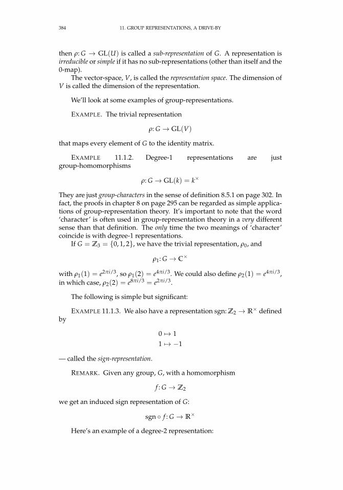
384 11. GROUP REPRESENTATIONS, A DRIVE-BY
then ρ: G → GL(U) is called a sub-representation of G. A representation isirreducible or simple if it has no sub-representations (other than itself and the0-map).
The vector-space, V, is called the representation space. The dimension ofV is called the dimension of the representation.
We’ll look at some examples of group-representations.
EXAMPLE. The trivial representation
ρ: G → GL(V)
that maps every element of G to the identity matrix.
EXAMPLE 11.1.2. Degree-1 representations are justgroup-homomorphisms
ρ: G → GL(k) = k×
They are just group-characters in the sense of definition 8.5.1 on page 302. Infact, the proofs in chapter 8 on page 295 can be regarded as simple applica-tions of group-representation theory. It’s important to note that the word‘character’ is often used in group-representation theory in a very differentsense than that definition. The only time the two meanings of ‘character’coincide is with degree-1 representations.
If G = Z3 = 0, 1, 2, we have the trivial representation, ρ0, and
ρ1: G → C×
with ρ1(1) = e2πi/3, so ρ1(2) = e4πi/3. We could also define ρ2(1) = e4πi/3,in which case, ρ2(2) = e8πi/3 = e2πi/3.
The following is simple but significant:
EXAMPLE 11.1.3. We also have a representation sgn: Z2 → R× definedby
0 7→ 11 7→ −1
— called the sign-representation.
REMARK. Given any group, G, with a homomorphism
f : G → Z2
we get an induced sign representation of G:
sgn f : G → R×
Here’s an example of a degree-2 representation:
11.1. INTRODUCTION 385
EXAMPLE 11.1.4. Let G = S3 and define
ρ(1) =[
1 00 1
]ρ((1, 2)) =
[− 1
2
√3
2√3
212
]
ρ((1, 3)) =
[− 1
2 −√
32
−√
32
12
]
ρ((2, 3)) =[
1 00 −1
]ρ((1, 2, 3)) =
[− 1
2 −√
32√
32 − 1
2
]
ρ((1, 3, 2)) =
[− 1
2
√3
2−√
32 − 1
2
]
This has a geometric interpretation: Let ω = e2πi/3 = − 12 +
√3
2 be a prim-itive cube root of 1. Then the three cube roots of 1 are 1, ω, ω2 and forma triangle in C, which we identify with R2. If we number these three roots,1, 2, and 3, respectively, S3 permutes these points via the matrices givenabove.
We can also give representations for Sn:
EXAMPLE 11.1.5. Let V be a vector space over k with basis-elementsb1, . . . , bn. Then we can define a representation for Sn by having it per-mute the basis elements. This representation has two sub-representations,V1 and T given by
V1 =
n
∑i=1
aibi
∣∣∣∣ai ∈ k and a1 = a2 = · · · = an
Tn =
n
∑i=1
aibi
∣∣∣∣ai ∈ k andn
∑i=1
ai = 0
Tn is called the standard representation of Sn.
To give a more modern definition of group-representations, we need torecall the concept of a group-ring — see 5.1.6 on page 109, in our case thegroup-ring kG and modules (see section 6.3 on page 220). Since k is a field,these are also algebras as in definition 7.1.4 on page 260 and often calledgroup-algebras.
DEFINITION 11.1.6. Let kG-mod and Vk be the categories of left kG-modules and vector-spaces over k, respectively. Define the forgetful functor(see example 10.3.2 on page 346) that maps a kG-module to its underlyingvector-space over k:
g: kG-mod→ Vk
386 11. GROUP REPRESENTATIONS, A DRIVE-BY
Given a vector-space, V, over a field, k, a representation of a group G over Vis a (left) kG-module, M, with g(M) = V. A homomorphism of representationsis just a kG-module homomorphism
f : M1 → M2
An isomorphism is a homomorphism that is an isomorphism of vectorspaces. A representation, M, is faithful if it contains a submodule isomor-phic to kG. An irreducible representation, M, has no sub-modules, otherthan M and the 0-submodule.
REMARK. Note that any module over kG is automatically a vector-space over k.
DEFINITION 11.1.7. If
ρ: G → GL(V)
is a representation of a group, G, define
VG = x ∈ V|ρ(g)(x) = x for all g ∈ Gthe G-stable subspace of V.
REMARK. Compare this with definition 13.3.1 on page 451.
We immediately have:
LEMMA 11.1.8 (Schur’s Lemma). If f : M1 → M2 is a homomorphism ofirreducible representations of a group, G, over a field, k, then f is either an iso-morphism or the 0-map. If follows that the ring, HomkG(M1, M1) = D, is adivision ring. If k is algebraically closed then HomkG(M1, M1) = k, so everyhomomorphism f : M1 → M1 is multiplication by a scalar in k.
PROOF. The kernel of f is a submodule of M1. Since M1 is irreducible,this must either be the 0-module or all of M1. If it is not all of M1, then itsimage in M2 is a submodule. Therefore its image must be all of M2. Thisalso implies that any homomorphism f : M1 → M1 must be the zero-mapor an isomorphism, which implies that HomkG(M1, M1) is a division-ring(multiplication is composition, and every nonzero element has an inverse).
If k is algebraically closed, f has an eigenvalue, λ, in k and
f − λ · I: M1 → M1
is a homomorphism that has a kernel. The first part of this lemma impliesthat f − λ · I = 0, so f = λ · I.
Issai Schur, 1875 – 1941, was a Russian mathematician who worked in Ger-many for most of his life. He studied at the University of Berlin.As a student of Ferdinand Georg Frobenius, he worked on group represen-tations, but also in combinatorics and number theory and even theoreticalphysics. He is best known for his result on the existence of the Schur de-composition and for his work on group representati ons (lemma 11.1.8).
In analogy with group theory (definition 4.4.14 on page 47), we define
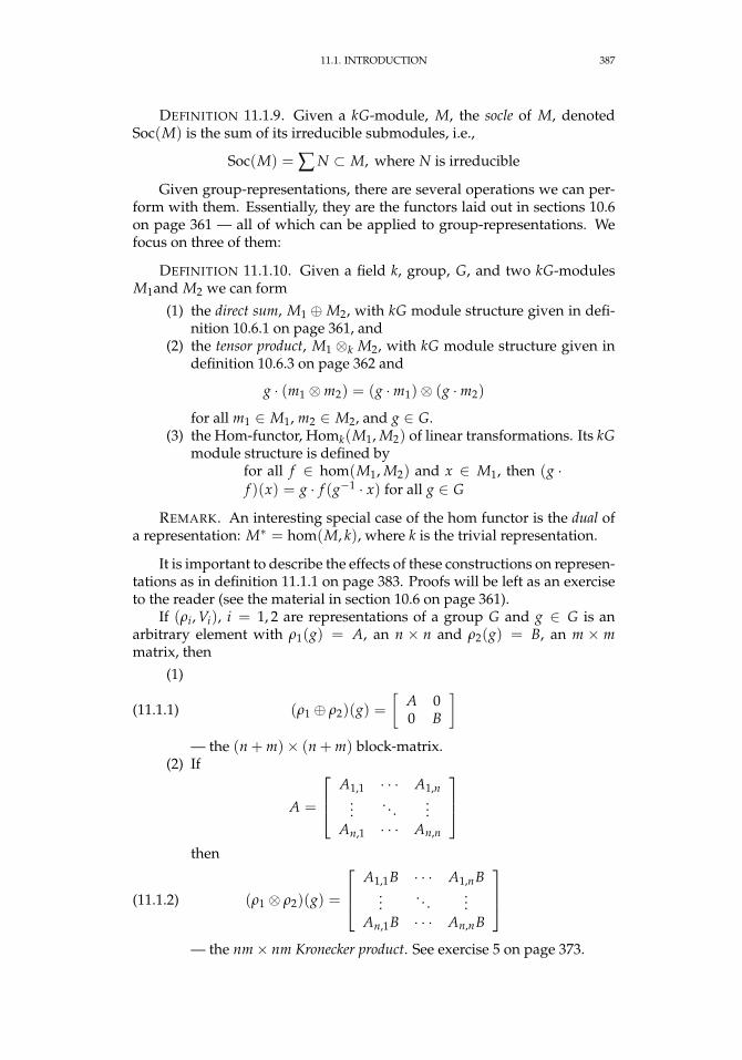
11.1. INTRODUCTION 387
DEFINITION 11.1.9. Given a kG-module, M, the socle of M, denotedSoc(M) is the sum of its irreducible submodules, i.e.,
Soc(M) = ∑ N ⊂ M, where N is irreducible
Given group-representations, there are several operations we can per-form with them. Essentially, they are the functors laid out in sections 10.6on page 361 — all of which can be applied to group-representations. Wefocus on three of them:
DEFINITION 11.1.10. Given a field k, group, G, and two kG-modulesM1and M2 we can form
(1) the direct sum, M1 ⊕M2, with kG module structure given in defi-nition 10.6.1 on page 361, and
(2) the tensor product, M1 ⊗k M2, with kG module structure given indefinition 10.6.3 on page 362 and
g · (m1 ⊗m2) = (g ·m1)⊗ (g ·m2)
for all m1 ∈ M1, m2 ∈ M2, and g ∈ G.(3) the Hom-functor, Homk(M1, M2) of linear transformations. Its kG
module structure is defined byfor all f ∈ hom(M1, M2) and x ∈ M1, then (g ·f )(x) = g · f (g−1 · x) for all g ∈ G
REMARK. An interesting special case of the hom functor is the dual ofa representation: M∗ = hom(M, k), where k is the trivial representation.
It is important to describe the effects of these constructions on represen-tations as in definition 11.1.1 on page 383. Proofs will be left as an exerciseto the reader (see the material in section 10.6 on page 361).
If (ρi, Vi), i = 1, 2 are representations of a group G and g ∈ G is anarbitrary element with ρ1(g) = A, an n × n and ρ2(g) = B, an m × mmatrix, then
(1)
(11.1.1) (ρ1 ⊕ ρ2)(g) =[
A 00 B
]— the (n + m)× (n + m) block-matrix.
(2) If
A =
A1,1 · · · A1,n...
. . ....
An,1 · · · An,n
then
(11.1.2) (ρ1 ⊗ ρ2)(g) =
A1,1B · · · A1,nB...
. . ....
An,1B · · · An,nB
— the nm× nm Kronecker product. See exercise 5 on page 373.
388 11. GROUP REPRESENTATIONS, A DRIVE-BY
(3)
(11.1.3) Homk(ρ1, ρ2)(g) =
A1,1B · · · A1,nB...
. . ....
An,1B · · · An,nB
— a Kronecker product, where A =
(A−1)t, the transpose of the
inverse.
DEFINITION 11.1.11. A representation (or module) is called semisimpleif it is a direct sum of simple (i.e., irreducible) representations. A ring, R, iscalled left-semisimple if all left R-modules are semisimple.
EXERCISES.
1. Show that the definitions 11.1.1 on page 383 and 11.1.6 on page 385are mathematically equivalent.
2. Suppose M is a simple (i.e., irreducible) module over a ring, R. Showthat M is generated by a single element.
3. Show that the representations of S3 in example 11.1.4 on page 384and T3 in example 11.1.5 on page 385 (done over C) are isomorphic.
4. Show that the representations of S3 in example 11.1.4 on page 384and T3 in example 11.1.5 on page 385 (done over C) are irreducible.
5. If G is a finite group and (ρ, V) is a representation over C, show thatρ(g) is a diagonalizable matrix for every g ∈ G and its eigenvalues haveabsolute value 1.
6. Prove equation 11.1.3.
7. Suppose G is a group, k is a field, and M1 and M2 are two kG-modules. Show that
Homk(M1, M2)G = HomkG(M1, M2)
In other words, the stabilizer of the Hom-functor of two representations isthe group of homomorphisms of the representations.
8. Let V be a finite-dimensional vector space with a subspace W andsuppose
P: V →W
is a projection onto W with the property that P|W = 1: W → W. Show thatTr (P) = dim W.
9. Suppose ρ1, ρ2: G → GL(V) are two faithful representations of agroup G. If they are isomorphic, show that ρ1(G) and ρ2(G) are conjugatesubgroups of GL(V).
11.2. FINITE GROUPS 389
10. Suppose ρ1, ρ2: G → GL(V) are two faithful representations of agroup G. such that ρ1(G) and ρ2(G) are conjugate subgroups of GL(V).Show that there is an automorphism ϕ: G → G such that ρ1 is isomorphicto ρ2 ϕ.
11. Suppose a module M has two irreducible submodules U1, U2 suchthat
M = U1 + U2
Show thatM ∼= U1 ⊕U2
12. Show that a module, M, is semisimple if and only if every sub-module N ⊂ M has a complement, i.e. if there exists another module U suchthat
M ∼= N ⊕U
13. If a module, M, is semisimple and N ⊂ M is a submodule, showthat N and M/N are semisimple.
14. If R is a ring that is semisimple as a left R-module, show that all leftR-modules are semisimple.
11.2. Finite Groups
Representation-theory for finite groups is a vast subject, so we willbarely scratch the surface!
EXAMPLE 11.2.1. Consider the dihedral group, D2n with elements1, f , · · · , f n−1, r, r f , . . . , r f n−1, where f is rotation by 2π/n and r isreflection of the x-coordinate. We have representations over R:
the trivial representation that maps its 2n elements to 1. the sign representation that maps f k to 1 and r f k to −1, for k =
1, . . . , n− 1. and a two-dimensional representation, ρ, from its geometric de-
scription in example 4.5.16 on page 57:
ρ( f k) =
[cos 2πk
n − sin 2πkn
sin 2πkn cos 2πk
n
]ρ(r f k) =
[ − cos 2πkn sin 2πk
nsin 2πk
n cos 2πkn
]We begin with
THEOREM 11.2.2 (Maschke’s Theorem). Let G be a finite group and let kbe a field with the property that |G| is invertible in k. If M ⊂ N is an inclusion ofleft kG-modules, then there exists a submodule U ⊂ N with the property that
N ∼= M⊕U
390 11. GROUP REPRESENTATIONS, A DRIVE-BY
It follows that all representations of G over k are direct sums of irreducible repre-sentations.
REMARK. The condition on |G| and the field, k means that k must be ofcharacteristic 0 or, if it is of characteristic p 6= 0, that p - |G|.
The submodule (or sub-representation) U is called a complement of Min N.
This result implies that, to classify all representations, it is only neces-sary to classify the irreducible ones.
PROOF. Note that M ⊂ N is an inclusion of vector-spaces. Theo-rem 6.2.6 on page 164 implies that we can find a basis, b1, . . . , bm of Mthat extends to one, b1, . . . , bm, c1, . . . , ck,for N. It is easy to define a linearmap of vector-spaces
f : N → Mwhose restriction to M is the identity map: just map the bito themselvesand map each cj to an arbitrary bi or 0. Now we define
f (x) =1|G| ∑
g∈Gg−1 · f (g · x)
for all x ∈ N. First of all, f |M is still the identity map: if x ∈ M, we haveg · x ∈ M because M is a sub-kG module and f (g · x) = g · x so g−1g · x = x.
We claim that f is a kG-module homomorphism, i.e., we claim that, forany h ∈ G f (h · x) = h · f (x).
First, note that,
f (x) =1|G| ∑
g∈Gg−1 · f (g · x) = 1
|G| ∑g∈G
h−1g−1 · f (gh · x)
for any fixed element h ∈ G. This is because, as g cycles through all theelements of G, so will gh. We have
f (h · x) = 1|G| ∑
g∈Gg−1 · f (gh · x)
= h1|G| ∑
g∈Gh−1g−1 · f (gh · x)
= h · f (x)
It follows that we have a kG-module homomorphism
f : N → M
with f |M = 1: M → M. If U = ker f , then g = 1− f : N → U is a kG-module homomorphism with g|U = 1: U → U. It is not hard to see that
M ∩U = 0
and we get an isomorphism
( f , g)N → M⊕U
The conclusion follows from exercise 12 on the preceding page.
11.2. FINITE GROUPS 391
Heinrich Maschke (1853 – 1908) was a German mathematician whose mostwell-known accomplishment was Maschke’s theorem.He earned his Ph.D. degree from the University of Göttingen in 1880. Hecame to the United States in 1891, and took up an Assistant Professor posi-tion at the University of Chicago in 1892
The condition that the order of the group be invertible is necessary:
EXAMPLE 11.2.3. Let G = Zp, generated by g with gp = 1, and con-sider the two-dimensional representation on the vector-space, Zp ⊕ Zp,given by
ρ(g) =[
1 0x 1
]where x ∈ G and not equal to the identity. This has an invariant subspace[
01
]so it is not irreducible. On the other hand, it is not the direct sum of thisinvariant subspace with any other one-dimensional representation so it vi-olates Maschke’s Theorem.
Given the importance of irreducible representations, we should have acriterion for irreducibility:
PROPOSITION 11.2.4. A representation, M, of a (not necessarily finite)group, G is irreducible if and only if, for every nonzero v ∈ M, the set of vectors
S = g · v|∀g ∈ Gspans M.
PROOF. If x ∈ G, we claim that x · Span(S) = Span(S). This is because,if g runs over all the elements of G so does x · g. It follows that Span(S) is asub-representation (or submodule). If Span(S) 6= M, then M has a propersub-representation and is not irreducible.
DEFINITION 11.2.5. If V is a vector-space, ρ: G → GL(V) is a represen-tation, and n ∈ Z≥0,define
V⊕n =
0 if n = 0⊕n
i=1 V otherwiseor
ρ⊕n =
0 if n = 0⊕n
i=1 ρ otherwise
Maschke’s Theorem shows that representations can be “factored”:
PROPOSITION 11.2.6. If G is a finite group, let ιj be a list of its irreduciblerepresentations over C. If ρ: G → GL(V) is a finite-dimensional representation ofG over C, there exists an isomorphism
(11.2.1) ρ→ ι⊕m11 ⊕ ι⊕m2
2 ⊕ · · ·for some integers mi ∈ Z≥0.

392 11. GROUP REPRESENTATIONS, A DRIVE-BY
PROOF. If ρ is irreducible, we’re done. Otherwise, Maschke’s Theorem( 11.2.2 on page 389) implies that ρ = ρ1 ⊕ ρ2. If we repeatedly apply thisreasoning to the summands, we eventually get a direct sum of irreduciblerepresentations. Exercise 1 on page 360 implies that we can rearrange thesesummands to the form in equation 11.2.1 on the previous page.
The reasoning used in Schur’s Lemma ( 11.1.8 on page 386) implies that
LEMMA 11.2.7. Let ξ be a representation of a group, let ι be an irreduciblerepresentation of the same group, and let
f : ι→ ξ
be a homomorphism. Then there are two possibilities:(1) f is an isomorphism of ι with an imbedded sub-representation ι ⊂ ξ,or(2) f is the zero-map.
This implies that the factorization in proposition 11.2.6 on the previouspage is unique:
COROLLARY 11.2.8. If G is a finite group, let ιj be a list of its irreduciblerepresentations over C. The representations ι⊕m1
1 ⊕ ι⊕m22 ⊕ · · · and ι⊕n1
1 ⊕ ι⊕n22 ⊕
· · · are isomorphic if and only if mi = ni for all i.
PROOF. Let pi: ι⊕n11 ⊕ ι⊕n2
2 ⊕ · · · → ι⊕mii be the projection.
Lemma 11.2.7 implies that, given any homomorphism
f : ι⊕m11 ⊕ ι⊕m2
2 ⊕ · · · → ι⊕n11 ⊕ ι⊕n2
2 ⊕ · · ·
the composite pi f |ι⊕mjj = 0: ι
⊕mjj → ι
⊕mii whenever i 6= j. This means
that f(
ι⊕mjj
)⊂ ι⊕njj for all j. This can be an isomorphism if and only if
mj = nj.
The following result will be useful in characterizing group-rings:
LEMMA 11.2.9. If R is a ring,
HomR(R, R) ∼= Rop
where Rop is the opposite ring to R — it has the same elements as R but r1 · r2 inRop is equal to r2 · r1 in R.
REMARK. Of course (Rop)op = R.
PROOF. A homomorphism f ∈ HomR(R, R) is completely determinedby where it sends 1 ∈ R — i.e., f (x) = x · f (1). We define
g: HomR(R, R)→ Rop
f 7→ f (1)
We need Rop becausef1 f2 7→ f2(1) · f1(1)
It is straightforward to verify that g is an isomorphism.
This leads to an interesting structural result:
11.2. FINITE GROUPS 393
THEOREM 11.2.10 (Artin-Wedderburn). Suppose R is a finite-dimensionalalgebra over a field, k, with the property that
R = ι⊕n11 ⊕ · · · ⊕ ι⊕nm
m
where the ιj are pairwise non-isomorphic irreducible left R-modules (left-idealsof R). Then there is an isomorphism
R ∼= Mn1(D1)⊕ · · · ⊕Mnm(Dm)
where the Dj = HomR(ιj, ιj)op are division-algebras and Mn(D) is the ring of
n× n matrices with entries in D — see example 5.1.5 on page 109.If k is algebraically closed, all the Di are equal to k, and
dimk ιj = nj
PROOF. We will use lemma 11.2.9 on the facing page and computeHomR(R, R)op = R. Note that, in any homomorphism
ι⊕n11 ⊕ · · · ⊕ ι⊕nm
m → ι⊕n11 ⊕ · · · ⊕ ι⊕nm
m
the image of any summand ι⊕njj will lie entirely in ι
⊕njj , by Schur’s Lemma
( 11.1.8 on page 386). Lemma 11.2.9 on the facing page implies that
Rop = HomR(R, R) = HomR(ι⊕n11 , ι⊕n1
1 )⊕ · · · ⊕HomR(ι⊕nmm , ι⊕nm
m )
FurthermoreHomR(ι
⊕njj , ι
⊕njj )
is the ring of nj × nj matrices with entries in HomR(ιj, ιj) = Dopj by Schur’s
Lemma again. The (j, i)th entry in this matrix will be a map from the ith
summand in the domain to the jthsummand in the range. We get
Rop ∼= Mn1(Dop1 )⊕ · · · ⊕Mnk (Dop
k )
The result follows by taking the opposite of everything in sight and notingthat Mni (Dop
i )op = Mni (Di).The final statement follows from
dimk Mnj(k) = n2j = nj · dimk ιj
The reasoning used in solving exercise 14 on page 389 implies that:
COROLLARY 11.2.11. Suppose R is a finite-dimensional semisimple algebraover a field, k, with the property that
R = ι⊕n11 ⊕ · · · ⊕ ι⊕nm
m
where the ιj are pairwise non-isomorphic irreducible left R-modules (left-idealsof R). Then the set ι1, . . . , ιm is a complete set of irreducible (simple) modulesover R. If k is algebraically closed, we have nj = dimk ιj and
dimk R = n21 + · · ·+ n2
m
394 11. GROUP REPRESENTATIONS, A DRIVE-BY
REMARK. Maschke’s Theorem ( 11.2.2 on page 389) implies that thehypotheses are satisfied if R = kG for some finite group, G, and k is a fieldof characteristic that doesn’t divide |G|. If k is also algebraically closed, thelast formula implies that
|G| = n21 + · · ·+ n2
m
which limits the number of possible irreducible representations and theirdimensions.
PROOF. All R-modules are quotients of free R-modules(proposition 6.3.10 on page 223), which are direct sums of copies of R. Itfollows that all of the irreducible modules that can occur in any R-modulemust already be present in R itself.
EXERCISES.
1. If k is a field and Mn(k) is the ring of n × n matrices over k, showthat
Mn(k) ∼= Mn(k)op
2. Show that the opposite of a matrix ring over a division-algebra isalso a matrix-ring over a division algebra. Conclude that a left-semisimplealgebra is also right-semisimple, so we may simply call them semisimple.
11.3. Characters
Now we will explore invariants of representations. These are easily-computed quantities that can characterize a representation up to isomor-phism.
EXERCISE 11.3.1. Show that the standard representation of Sn in exam-ple 11.1.5 on page 385 is irreducible.
Given a matrix, A, representing a linear transformation
f : V → V
note that the trace (see definition 6.2.53 on page 194), Tr (A), is a well-defined invariant of f . In other words, it does not depend on the basisfor V used to compute Tr (A) . This is because Tr
(P−1 AP
)= Tr (A) for any
invertible matrix P — see exercise 18 on page 199.With this in mind, we define
DEFINITION 11.3.2. Given a vector-space, V, over a field, k, and a rep-resentation of a group G , (ρ, V), define the character of the representationto be a function
ξ: G → kgiven by ξ(g) = Tr (ρ(g)).
11.3. CHARACTERS 395
REMARK. The character of a representation is almost never a homo-morphism (unless the representation is of degree 1)!
Isomorphic representations have the same characters (again, considerexercise 18 on page 199).
Recall the equivalence relation of conjugacy defined inproposition 4.7.11 on page 78. This results in a group, G, being subdividedinto conjugacy classes as in equation 4.7.2 on page 78
G =⊔
Ci
where all elements in each of the Ci are conjugate to each other.
DEFINITION 11.3.3. Let G be a finite group, let S = C1, . . . , Cn be itsconjugacy classes, and let k be a field. A class function of G is just a function
f : S→ k
Exercise 18 on page 199 immediately implies that
PROPOSITION 11.3.4. Characters of group-representations are class func-tions.
EXAMPLE 11.3.5. Consider the representation of S3 in example 11.1.4on page 384. Since conjugacy in Sn is determined by cycle-structure (seecorollary 4.5.12 on page 54 and exercise 3 on page 58) we have three conju-gacy classes in S3
C0 = 1C1 = (1, 2), (1, 3), (2, 3)C3 = (1, 2, 3), (1, 3, 2)
and the character of that representation is given by
ξ(C0) = 2
ξ(C1) = 0
ξ(C2) = −1
DEFINITION 11.3.6. A finite group’s character table has rows corre-sponding to irreducible representations and columns corresponding to con-jugacy classes.
EXAMPLE 11.3.7. Here’s a character table for S3:C0 = 1 C1 = (1, 2), (1, 3), (2, 3) C2 = (1, 2, 3), (1, 3, 2)
triv 1 1 1sgn 1 −1 1std 2 0 −1Here, triv is the one-dimensional trivial representation that sends all ele-
ments of S3 to the identity, sgn is the one-dimensional sign-representation, and std is the two-dimensional standard representation in
examples 11.1.4 on page 384 and 11.1.5 on page 385.

396 11. GROUP REPRESENTATIONS, A DRIVE-BY
REMARK. It isn’t obvious (but true) that these are all of the irreduciblerepresentations of S3. We can make other observations that turn out not tobe mere coincidences:
(dim triv)2 + (dim sgn)2 + (dim std)2 = 1 + 1 + 4 = |S3|. Com-pare this to the Artin-Wedderburn Theorem, 11.2.10 on page 393.
If ξ1, ξ2 are two distinct representations from the character tableabove, then
∑g∈S3
ξ1(g)ξ2(g) = 0
The reasoning used in Maschke’s Theorem can be generalized
LEMMA 11.3.8. Let ρ: G → GL(V) be a representation of a finite group anddefine
T =1|G| ∑
g∈Gρ(g)
ThenT: V → VG
is a projection onto the stable subspace of V (see definition 11.1.7 on page 386).
PROOF. If x ∈ V is in the image of T then there exists y ∈ V such that
x =1|G| ∑
g∈Gρ(g)(y)
and
ρ(h)(x) = ρ(h)1|G| ∑
g∈Gρ(g)(y)
=1|G| ∑
g∈Gρ(h)ρ(g)(y)
=1|G| ∑
g∈Gρ(hg)(y)
= x
since hg runs over all the elements of G. On the other hand, it is not hardto see that x ∈ VG implies that T(x) = x, so the conclusion follows.
COROLLARY 11.3.9. Let ρ: G → GL(V) be a representation of a finite groupwith character ξ: G → C. Then
1|G| ∑
g∈Gξ(g) = dim VG
PROOF. We use lemma 11.3.8 and the conclusion of exercise 8 onpage 388 to conclude that
1|G| Tr
(1|G| ∑
g∈Gρ(g)
)= dim VG
11.3. CHARACTERS 397
But
Tr
(1|G| ∑
g∈Gρ(g)
)=
1|G| ∑
g∈GTr (ρ(g))
=1|G| ∑
g∈Gξ(g)
For the remainder of this chapter, we’ll assume that k = C and define
DEFINITION 11.3.10. If, ξ1, ξ2, are characters of representations of a fi-nite group, G, over C, we define the inner product
〈ξ1, ξ2〉 =1|G| ∑
g∈Gξ1(g)ξ2(g)
=1|G| ∑
c∈S|c| · ξ1(c)ξ2(c)(11.3.1)
where S is the set of conjugacy-classes in G and |s| is the number of ele-ments in the conjugacy-class, s.
REMARK. Note that|c||G| =
1|ZG(c)|
where |ZG(c)| is the the number elements that commute with g (the central-izer of g) — see corollary 4.7.13 on page 79. We can rewrite equation 11.3.1as
(11.3.2) 〈ξ1, ξ2〉 = ∑c∈S
ξ1(c)ξ2(c)|ZG(c)|
To understand the significance of this inner product, we need
PROPOSITION 11.3.11. Let ρ1, ρ2 be two representations of a finite group Gover C with characters ξ1, ξ2, respectively. Then the character of Homk(ρ1, ρ2) is
ξ1 · ξ2
PROOF. Equation 11.1.3 on page 388 implies that the matrix forHomk(ρ1, ρ2)(g) is the Kronecker product of the transpose of the inverseof the matrix for ρ1(g) with that of ρ2(g) for all g ∈ G. It follows that thetraces satisfy
Tr (Hom(ρ1, ρ2)(g)) = Tr(
ρ1(g)−1)· ξ2(g)
since transposing leaves the trace unchanged. Exercise 211 on page 511shows that ρ1(g) is diagonalizable and that its eigenvalues, λ1, . . . , λkare
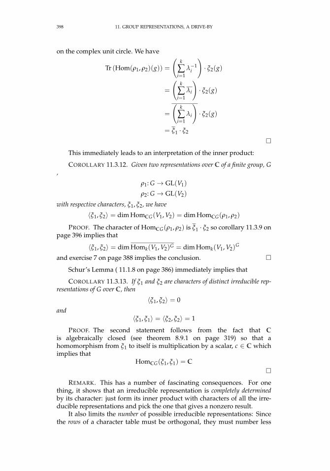
398 11. GROUP REPRESENTATIONS, A DRIVE-BY
on the complex unit circle. We have
Tr (Hom(ρ1, ρ2)(g)) =
(k
∑i=1
λ−1i
)· ξ2(g)
=
(k
∑i=1
λi
)· ξ2(g)
=
(k
∑i=1
λi
)· ξ2(g)
= ξ1 · ξ2
This immediately leads to an interpretation of the inner product:
COROLLARY 11.3.12. Given two representations over C of a finite group, G,
ρ1: G → GL(V1)
ρ2: G → GL(V2)
with respective characters, ξ1, ξ2, we have
〈ξ1, ξ2〉 = dim HomCG(V1, V2) = dim HomCG(ρ1, ρ2)
PROOF. The character of HomCG(ρ1, ρ2) is ξ1 · ξ2 so corollary 11.3.9 onpage 396 implies that
〈ξ1, ξ2〉 = dim Homk(V1, V2)G = dim Homk(V1, V2)G
and exercise 7 on page 388 implies the conclusion.
Schur’s Lemma ( 11.1.8 on page 386) immediately implies that
COROLLARY 11.3.13. If ξ1 and ξ2 are characters of distinct irreducible rep-resentations of G over C, then
〈ξ1, ξ2〉 = 0
and〈ξ1, ξ1〉 = 〈ξ2, ξ2〉 = 1
PROOF. The second statement follows from the fact that C
is algebraically closed (see theorem 8.9.1 on page 319) so that ahomomorphism from ξ1 to itself is multiplication by a scalar, c ∈ C whichimplies that
HomCG(ξ1, ξ1) = C
REMARK. This has a number of fascinating consequences. For onething, it shows that an irreducible representation is completely determinedby its character: just form its inner product with characters of all the irre-ducible representations and pick the one that gives a nonzero result.
It also limits the number of possible irreducible representations: Sincethe rows of a character table must be orthogonal, they must number less
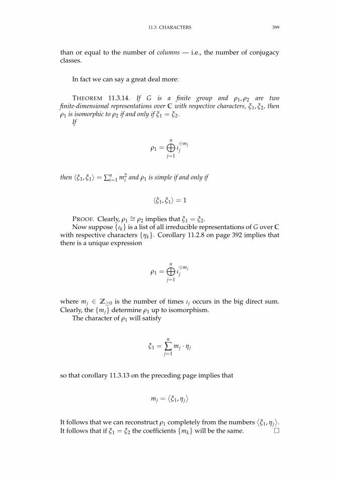
11.3. CHARACTERS 399
than or equal to the number of columns — i.e., the number of conjugacyclasses.
In fact we can say a great deal more:
THEOREM 11.3.14. If G is a finite group and ρ1, ρ2 are twofinite-dimensional representations over C with respective characters, ξ1, ξ2, thenρ1 is isomorphic to ρ2 if and only if ξ1 = ξ2.
If
ρ1 =n⊕
j=1
ι⊕mjj
then 〈ξ1, ξ1〉 = ∑ni=1 m2
i and ρ1 is simple if and only if
〈ξ1, ξ1〉 = 1
PROOF. Clearly, ρ1∼= ρ2 implies that ξ1 = ξ2.
Now suppose ιk is a list of all irreducible representations of G over C
with respective characters ηk. Corollary 11.2.8 on page 392 implies thatthere is a unique expression
ρ1 =n⊕
j=1
ι⊕mjj
where mj ∈ Z≥0 is the number of times ιj occurs in the big direct sum.Clearly, the mj determine ρ1 up to isomorphism.
The character of ρ1 will satisfy
ξ1 =n
∑j=1
mj · ηj
so that corollary 11.3.13 on the preceding page implies that
mj =⟨ξ1, ηj
⟩It follows that we can reconstruct ρ1 completely from the numbers
⟨ξ1, ηj
⟩.
It follows that if ξ1 = ξ2 the coefficients mk will be the same.
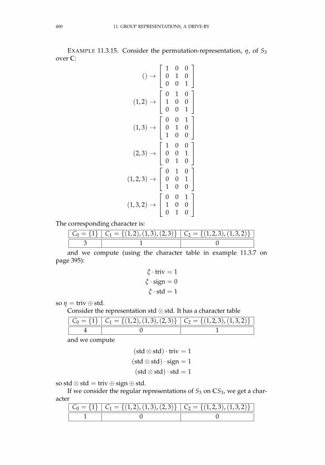
400 11. GROUP REPRESENTATIONS, A DRIVE-BY
EXAMPLE 11.3.15. Consider the permutation-representation, η, of S3over C:
()→ 1 0 0
0 1 00 0 1
(1, 2)→
0 1 01 0 00 0 1
(1, 3)→
0 0 10 1 01 0 0
(2, 3)→
1 0 00 0 10 1 0
(1, 2, 3)→
0 1 00 0 11 0 0
(1, 3, 2)→
0 0 11 0 00 1 0
The corresponding character is:
C0 = 1 C1 = (1, 2), (1, 3), (2, 3) C2 = (1, 2, 3), (1, 3, 2)3 1 0
and we compute (using the character table in example 11.3.7 onpage 395):
ξ · triv = 1ξ · sign = 0
ξ · std = 1
so η = triv⊕ std.Consider the representation std⊗ std. It has a character table
C0 = 1 C1 = (1, 2), (1, 3), (2, 3) C2 = (1, 2, 3), (1, 3, 2)4 0 1
and we compute
(std⊗ std) · triv = 1
(std⊗ std) · sign = 1
(std⊗ std) · std = 1
so std⊗ std = triv⊕ sign⊕ std.If we consider the regular representations of S3 on CS3, we get a char-
acterC0 = 1 C1 = (1, 2), (1, 3), (2, 3) C2 = (1, 2, 3), (1, 3, 2)
1 0 0

11.3. CHARACTERS 401
so CS3 = triv⊕ sign⊕ std⊕ std.
Our next project will be to determine the number of isomorphismclasses of irreducible representations. We begin by extending the conceptof center from group-theory (definition 4.4.9 on page 46) to ring-theory:
DEFINITION 11.3.16. If R is a ring, the center of R, denoted Z(R) is theset of elements that commute with all elements of R, i.e.
Z(R) = r ∈ R|sr = rs, for ∀s ∈ RWe leave the proof of the following as an exercise to the reader:
PROPOSITION 11.3.17. If G is a finite group and k is a field, then
Z(kG) =
r ∈ kG|g−1rg = r, for ∀g ∈ G
COROLLARY 11.3.18. Let G be a finite group, let k be a field, let S =C1, . . . , Cn be the conjugacy classes of G, and let
σi = ∑g∈Ci
g
Then σi ∈ Z(kG) for i = 1, . . . n. It follows that
dimk Z(kG) ≥ n
— the number of conjugacy classes.
PROOF. Since all the elements of Ci are conjugate to each other, conju-gating them by group-elements just permutes them and leaves the sum un-changed. Since distinct σi are linearly independent (for instance, Ci ∩ Cj =∅ for i 6= j), the conclusion follows.
It’s easy to characterize the center of a matrix-ring:
PROPOSITION 11.3.19. Let k be a field and let n > 0 be an integer. Then
Z(Mn(k)) = k · I— scalar multiples of the identity matrix.
PROOF. Let Ei,j be the n × n matrix with 1 in position i, j and 0 else-where. If A is an arbitrary n× n matrix, then
Ei,j A = matrix whose ith-row is the jth row of A
AEi,j = matrix whose ith-column is the jth column of A
The only way these can be equal is if every row and column of A has, atmost, a single nonzero element — and these elements (in distinct rows andcolumns) are equal.
Now we can prove our main result:
THEOREM 11.3.20. If G is a finite group, then
dimk Z(CG) = the number of distinct simple representations of G= the number of conjugacy classes of G
It follows that character-tables are always square. Furthermore, the σi definedin corollary 11.3.18 are a basis for Z(kG).
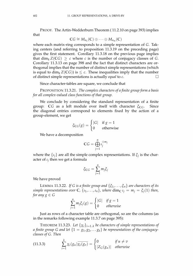
402 11. GROUP REPRESENTATIONS, A DRIVE-BY
PROOF. The Artin-Wedderburn Theorem ( 11.2.10 on page 393) impliesthat
CG ∼= Mn1(C)⊕ · · · ⊕Mnm(C)
where each matrix-ring corresponds to a simple representation of G. Tak-ing centers (and referring to proposition 11.3.19 on the preceding page)gives the first statement. Corollary 11.3.18 on the previous page impliesthat dimk Z(CG) ≥ c where c is the number of conjugacy classes of G.Corollary 11.3.13 on page 398 and the fact that distinct characters are or-thogonal implies that the number of distinct simple representations (whichis equal to dimk Z(CG)) is ≤ c. These inequalities imply that the numberof distinct simple representations is actually equal to c.
Since character-tables are square, we conclude that
PROPOSITION 11.3.21. The complex characters of a finite group form a basisfor all complex-valued class functions of that group.
We conclude by considering the standard representation of a finitegroup: CG as a left module over itself with character ξCG. Sincethe diagonal entries correspond to elements fixed by the action of agroup-element, we get
ξCG(g) =
|G| if g = 10 otherwise
We have a decomposition
CG =n⊕
j=1
ι⊕mjj
where the ιj are all the simple complex representations. If ξ j is the char-acter of ιj then we get a formula
ξCG =n
∑j=1
mjξ j
We have proved
LEMMA 11.3.22. If G is a finite group and ξ1, . . . , ξn are characters of itssimple representations over C, ι1, . . . , ιn, where dimC ιj = mj = ξ j(1) then,for any g ∈ G
n
∑j=1
mjξ j(g) =
|G| if g = 10 otherwise
Just as rows of a character table are orthogonal, so are the columns (asin the remarks following example 11.3.7 on page 395):
THEOREM 11.3.23. Let χii=1..k be characters of simple representations ofa finite group G and let 1 = g1, g2, . . . gk be representatives of the conjugacy-classes of G. Then
(11.3.3)k
∑i=1
χi(gu)χi(gv) =
0 if u 6= v|ZG(gu)| otherwise
11.3. CHARACTERS 403
Here, ZG(gj) is the centralizer of gj in G — see definition 4.7.12 on page 79.
PROOF. Let X be the k × k matrix for the character-table and let Z bethe k× k diagonal matrix
Z =
|ZG(g1)| 0 · · · 0
0 |ZG(g2)| · · ·...
......
. . . 00 · · · 0 |ZG(gk)|
Equation 11.3.2 on page 397 is equivalent to
XC−1Xt = I
where X is the complex conjugate. Since all matrices here are invertible, wecan write (
XC−1)−1
= Xt = CX−1
so thatXtX = C
which is equation 11.3.3 on the facing page.
Recall the concept of integral elements of a field developed in sec-tion 6.5 on page 249.
PROPOSITION 11.3.24. If G is a finite group the center, Z(ZG), is integralover Z. If g1 = 1, . . . , gk are representatives of the conjugacy-classes of G thengi ∈ Z(ZG) are integral over Z, where g is the sum of all the elements conjugateto g. If λ1, . . . , λk are algebraic integers over Z, then
k
∑i=1
λi gi
is an algebraic integer over Z. If f : G → C is a class function then
z = ∑g∈G
f (g) · g
is in Z(CG).
REMARK. In light of definition 6.5.1 on page 249, this means it’s aroot of a monic polynomial with integer coefficients. Proposition 6.5.5 onpage 251 shows that algebraic integers form a ring.
PROOF. That elements of Z(ZG) are integral over Z follows from thefact that ZG is a finitely-generated Z-module, and Z(ZG) is a submodule,so also finitely generated — see proposition 6.5.2 on page 249. The state-ment about the gi follows from proposition 11.3.17 on page 401. The secondstatement follows from the fact that algebraic integers form a ring — again,see proposition 6.5.2 on page 249.
The statement about z follows from the fact that we can rewrite z ask
∑i=1
f (gi) · gi
since f is constant over elements of a conjugacy class.
404 11. GROUP REPRESENTATIONS, A DRIVE-BY
PROPOSITION 11.3.25. If ρ is a d-dimensional simple representation of afinite group, G, over C and x ∈ Z(CG) then
ρ(x) = λ · Ifor some λ ∈ C. in fact
ρ(x) =1d
Tr (ρ(x)) · IIf x = ∑g∈G αgg, then
ρ(x) = ∑g∈G
αgχ(g) · I
where χ is the character of ρ.
PROOF. Since x commutes with every element of G, ρ(x) commuteswith all of ρ(g) for any g ∈ G — therefore the homomorphism
ρ(x): Cd → Cd
of vector-spaces is actually a homomorphism of CG-modules. Schur’sLemma, 11.1.8 on page 386, implies that it is of the form λ · I. The finalconclusion follows from the fact that
Tr (λ · I) = d · λ
We also conclude that
THEOREM 11.3.26. The degrees of the simple complex representations of afinite group all divide the order of the group.
PROOF. Let χ be the character of a degree-d simple complex represen-tation, ρ. The final statement of proposition 11.3.24 on the preceding pageimplies that
x = ∑g∈G
χ(g−1)g
is in Z(CG). Proposition 11.3.25 implies that
ρ(x) =1d ∑
g∈Gχ(g−1)χ(g) · I = 1
d
(∑
g∈G1
)I =|G|d· I
Since x is integral over Z (by Proposition 11.3.24 on the preceding page)and |G|/d ∈ Q, we conclude that |G|/d ∈ Z so d
∣∣ |G|.
11.4. EXAMPLES 405
EXERCISES.
1. If G is a finite group and ρ: G → Ck is a representation, show thatρ(g) is diagonalizable for any g ∈ G.
2. If G is a finite group and ρ: G → Ck is a representation with characterχ, and g ∈ G is of order n, show that χ(g) is a sum of nth roots of unity(including roots whose order divides n).
3. If G is a finite group and ρ: G → Ck is a representation with char-acter χ, and |χ(1)| = |χ(g)| for some element g ∈ G, show that ρ(g) ismultiplication by a scalar (root of unity)
4. If χ is the character of a complex representation of a finite group, G,show that χ(g−1) = χ(g) for all g ∈ G.
5. Show that, if every element of a finite group G is conjugate to itsinverse, every complex character is real-valued. Conversely, show that ifevery complex character of G is real-valued, then every element of G isconjugate to its inverse.
11.4. Examples
We have seen a character-table for S3 in example 11.3.7 on page 395.Now we will do S4. It is well-known that conjugacy-class of an element
of a symmetric group is determined by its cycle-structure — see exercise 3on page 58. Our table will look like
() (∗, ∗) (∗, ∗)(∗, ∗) (∗, ∗, ∗) (∗, ∗, ∗, ∗)size 1 6 3 8 6triv 1 1 1 1 1sgn 1 −1 1 1 −1
where the second row is the size of the respective conjugacy classes.We consider the representation where S4 acts on C4 by permuting the
axes. The character is equal to the number of axes fixed by a given permu-tation, so we get
() (∗, ∗) (∗, ∗)(∗, ∗) (∗, ∗, ∗) (∗, ∗, ∗, ∗)size 1 6 3 8 6
perm 4 2 0 1 0This representation is not simple: it contains an invariant subspace iso-
morphic to the trivial representation. It is the representation that permutesthe axes in the three-dimensional subspace of C4 with ∑4
i=1 xi = 0. Wesubtract the trivial character from perm to get
() (∗, ∗) (∗, ∗)(∗, ∗) (∗, ∗, ∗) (∗, ∗, ∗, ∗)size 1 6 3 8 6std 3 1 −1 0 −1
406 11. GROUP REPRESENTATIONS, A DRIVE-BY
The computation 〈std, std〉 = 1 shows that it is simple (seetheorem 11.3.14 on page 399). It is not hard to see that
〈std⊗ sgn, std⊗ sgn〉 = 1
so our character-table has 4 rows() (∗, ∗) (∗, ∗)(∗, ∗) (∗, ∗, ∗) (∗, ∗, ∗, ∗)
size 1 6 3 8 6triv 1 1 1 1 1sgn 1 −1 1 1 −1std 3 1 −1 0 −1
std⊗ sgn 3 −1 −1 0 1To get the fifth representation, note that the subgroup
K = 1, (1, 2)(3, 4), (1, 3)(2, 4), (1, 4)(2, 3) ⊂ S4
is normal1. The quotient is isomorphic to S3 and the projection p: S4 → S3is given by
() 7→ ()
(1, 2) 7→ (1, 2)
(1, 2)(3, 4) 7→ ()
(1, 2, 3, 4) 7→ (1, 3)
(1, 2, 3) 7→ (1, 2, 3)
Any representation ρ: S3 → GL(V) gives rise to a representation of S4 bycomposition p ρ. It follows that the representation in the bottom row ofthe table in example 11.3.7 on page 395 gives rise to one of S4:
() (∗, ∗) (∗, ∗)(∗, ∗) (∗, ∗, ∗) (∗, ∗, ∗, ∗)size 1 6 3 8 6ξpæ 2 0 2 −1 0
A simple computation shows that⟨ξpæ, ξpæ
⟩= 1
so it is irreducible (or simple). We could also have come to this conclusionusing the fact that the representation of S3 was simple.
This completes our character-table for S4:() (∗, ∗) (∗, ∗)(∗, ∗) (∗, ∗, ∗) (∗, ∗, ∗, ∗)
size 1 6 3 8 6triv 1 1 1 1 1sgn 1 −1 1 1 −1std 3 1 −1 0 −1
std⊗ sgn 3 −1 −1 0 1ξpæ 2 0 2 −1 0
Based on the representations in example 11.2.1 on page 389, we get partof a character table over R for the dihedral group, D2n:
1Conjugation leaves its cycle-structure intact.
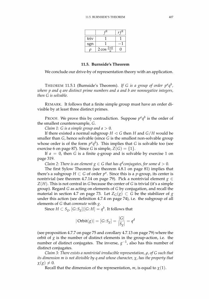
11.5. BURNSIDE’S THEOREM 407
f k r f k
triv 1 1sgn 1 −1
ρ 2 cos 2πkn 0
11.5. Burnside’s Theorem
We conclude our drive-by of representation theory with an application.
THEOREM 11.5.1 (Burnside’s Theorem). If G is a group of order paqb,where p and q are distinct prime numbers and a and b are nonnegative integers,then G is solvable.
REMARK. It follows that a finite simple group must have an order di-visible by at least three distinct primes.
PROOF. We prove this by contradiction. Suppose paqb is the order ofthe smallest counterexample, G.
Claim 1: G is a simple group and a > 0.If there existed a normal subgroup H C G then H and G/H would be
smaller than G, hence solvable (since G is the smallest non-solvable groupwhose order is of the form paqb). This implies that G is solvable too (seeexercise 6 on page 87). Since G is simple, Z(G) = 1.
If a = 0, then G is a finite q-group and is solvable by exercise 1 onpage 319.
Claim 2: There is an element g ∈ G that has qdconjugates, for some d > 0.The first Sylow Theorem (see theorem 4.8.1 on page 81) implies that
there’s a subgroup H ⊂ G of order pa. Since this is a p-group, its center isnontrivial (see theorem 4.7.14 on page 79). Pick a nontrivial element g ∈Z(H). This is not central in G because the center of G is trivial (it’s a simplegroup). Regard G as acting on elements of G by conjugation, and recall thematerial in section 4.7 on page 73. Let ZG(g) ⊂ G be the stabilizer of gunder this action (see definition 4.7.4 on page 74), i.e. the subgroup of allelements of G that commute with g.
Since H ⊂ Sg, [G: Sg]|[G: H] = qb. It follows that
|Orbit(g)| = [G: Sg] =|G||Sg|
= qd
(see proposition 4.7.7 on page 75 and corollary 4.7.13 on page 79) where theorbit of g is the number of distinct elements in the group-action, i.e. thenumber of distinct conjugates. The inverse, g−1, also has this number ofdistinct conjugates.
Claim 3: There exists a nontrivial irreducible representation, ρ, of G such thatits dimension m is not divisible by q and whose character, χ, has the property thatχ(g) 6= 0.
Recall that the dimension of the representation, m, is equal to χ(1).
408 11. GROUP REPRESENTATIONS, A DRIVE-BY
Let χ1, . . . , χk denote the irreducible characters of G, where χ1 is thetrivial character. Theorem 11.3.23 on page 402 implies that
k
∑i=1
χi(1)χi(g) = 0 = 1 +k
∑i=2
χi(1)χi(g) = 1 +k
∑i=2
χi(1)χi(g−1)
If all of the algebraic integers χi(g−1) are divisible by q then
−1q=
k
∑i=2
1q
χi(1)χi(g−1)
would be an algebraic integer, which it clearly isn’t.Claim 4: The complex number qdχ(g)/m is an algebraic integer.The number of conjugates of g is qd. Let g be the sum of all these conju-
gates; we have g ∈ Z(CG), by proposition 11.3.24 on page 403 and propo-sition 11.3.25 on page 404 implies that
ρ(g) =1m ∑
h∼gχ(h) · I
=qdχ(g)
m· I
(where h ∼ g means h is conjugate to g) and this is integral over Z.Claim 5: The complex number χ(g)/m is an algebraic integer.This is due to the fact that d - m, so we can find integers a and b such
thataqd + bm = 1
(see lemma 3.1.5 on page 14) which gives
χ(g)m
= aqdχ(g)
m+ bχ(g)
a sum of algebraic integers.Claim 6: |χ(g)| = m.Set ξ = χ(g)/m. Then the algebraic conjugates (see definition 3.1.5
on page 14) of ξ are all algebraic integers so their product N(ξ) (seelemma 7.5.11 on page 284) is also an algebraic integer. Since it is ± theconstant term of the minimal polynomial of ξ over Q, it is rational, hence0 6= N(ξ) ∈ Z.
Now χ(g) is the sum of the m eigenvalues of ρ(g), each of which is aroot of unity. The triangle inequality implies that |χ(g)| ≤ m, and Galoistheory implies that this is true of each of the algebraic conjugates of χ(g),so that all the algebraic conjugates of ξ have absolute value ≤ 1.
Consequently 0 6= |N(ξ)| ≤ 1. Since it must be an integer, we have|N(ξ)| = 1, which proves the claim.
Consider the set
H = h ∈ G||χ(h)| = mExercise 3 on page 405 implies that ρ(h) is multiplication by a scalar
(root of unity). This implies that H is a subgroup of G. Furthermore, it’sa normal subgroup since matrices λ · I commute with all other matrices. In
11.5. BURNSIDE’S THEOREM 409
fact, H/ ker ρ is abelian since it is equal to the image of H under ρ in thering of matrices — and diagonal matrices commute with each other.
Since H contains the element g, it is nontrivial. The simplicity of G thenimplies that H = G. Since ρ is not a trivial representation, the simplicity ofG implies that ker ρ = 1. This implies that G = H/ ker ρ is abelian, which isa contradiction.

CHAPTER 12
A little algebraic geometry
“Algebraic geometry seems to have acquired the reputation ofbeing esoteric, exclusive, and very abstract, with adherents whoare secretly plotting to take over all the rest of mathematics. Inone respect this last point is accurate.”
—David Mumford in [77].
12.1. Introduction
Algebraic geometry concerns itself with objects called algebraic varieties.These are essentially solution-sets of systems of algebraic equations.
Although restricting our attention to algebraic varieties might seemlimiting, it has long been known that more general objects like compactsmooth manifolds are diffeomorphic to real varieties — see [79]1 and [104].The paper [1] even shows that many piecewise-linear manifolds, includingones with no smooth structure are homeomorphic to real varieties.
The reader interested in more than a little bit of algebraic geometry isinvited to look at [99].
We begin with algebraic sets, whose geometric properties are completelycharacterized by a basic algebraic invariant called the coordinate ring. Themain objects of study — algebraic varieties — are the result of gluing to-gether multiple affine sets.
Throughout this discussion, k will denote a fixed algebraically closedfield (see definition 7.5.1 on page 281). In classical algebraic geometryk = C.
DEFINITION 12.1.1. An n-dimensional affine space, An = kn, regarded asa space in which geometric objects can be defined. An algebraic set, V (S), inkn is the set of common zeros of some set S of polynomials in k[X1, . . . , Xm]:
V (S) = (a1, . . . , an) ∈ An| f (a1, . . . , an) = 0 for all f (X1, . . . , Xn) ∈ SREMARK. It is not hard to see that if the set of polynomials is larger,
the set of common zeros will be smaller, i.e.,
S ⊂ S′ =⇒ V (S) ⊃ V(S′)
If a is the ideal generated by the polynomials in S, we haveV (a) = V (S) so algebraic sets are described as V (a) for some ideala ⊆ k[X1, . . . , Xm] (see definition 5.2.3 on page 111).
Recall that all ideals in k[X1, . . . , Xn] are finitely generated bytheorem 5.4.4 (the Hilbert Basis Theorem).
1Written by John Nash, the character of the film “A beautiful mind.”
411
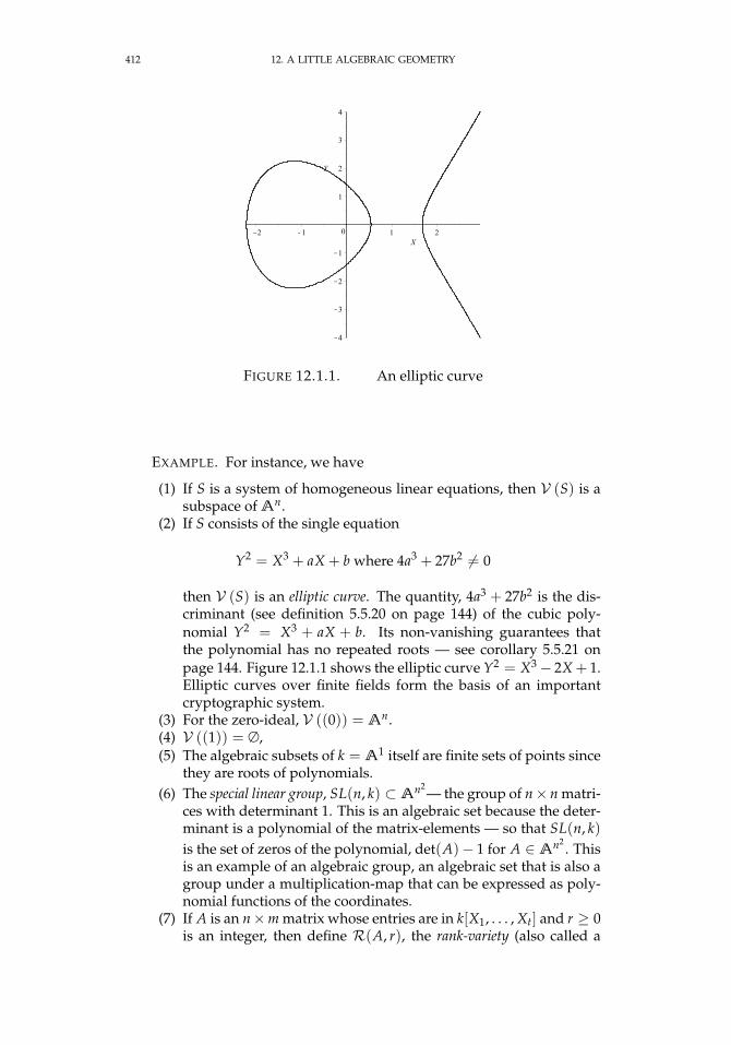
412 12. A LITTLE ALGEBRAIC GEOMETRY
FIGURE 12.1.1. An elliptic curve
EXAMPLE. For instance, we have
(1) If S is a system of homogeneous linear equations, then V (S) is asubspace of An.
(2) If S consists of the single equation
Y2 = X3 + aX + b where 4a3 + 27b2 6= 0
then V (S) is an elliptic curve. The quantity, 4a3 + 27b2 is the dis-criminant (see definition 5.5.20 on page 144) of the cubic poly-nomial Y2 = X3 + aX + b. Its non-vanishing guarantees thatthe polynomial has no repeated roots — see corollary 5.5.21 onpage 144. Figure 12.1.1 shows the elliptic curve Y2 = X3− 2X + 1.Elliptic curves over finite fields form the basis of an importantcryptographic system.
(3) For the zero-ideal, V ((0)) = An.(4) V ((1)) = ∅,(5) The algebraic subsets of k = A1 itself are finite sets of points since
they are roots of polynomials.(6) The special linear group, SL(n, k) ⊂ An2
— the group of n× n matri-ces with determinant 1. This is an algebraic set because the deter-minant is a polynomial of the matrix-elements — so that SL(n, k)is the set of zeros of the polynomial, det(A)− 1 for A ∈ An2
. Thisis an example of an algebraic group, an algebraic set that is also agroup under a multiplication-map that can be expressed as poly-nomial functions of the coordinates.
(7) If A is an n×m matrix whose entries are in k[X1, . . . , Xt] and r ≥ 0is an integer, then define R(A, r), the rank-variety (also called a
12.1. INTRODUCTION 413
determinantal variety),
R(A, r) =
At if r ≥ min(n, m)
p ∈ At such that rank(A(p)) ≤ r
This is an algebraic set because the statement that the rank of A is≤ r is the same as saying the determinants of all (r + 1)× (r + 1)sub-matrices are 0.
Here are some basic properties of algebraic sets and the ideals that generatethem:
PROPOSITION 12.1.2. Let a, b ⊂ k[X1, . . . , Xn] be ideals. Then(1) a ⊂ b =⇒ V (a) ⊃ V (b)(2) V (ab) = V (a∩ b) = V (a) ∪ V (b)(3) V (∑ ai) =
⋂ V (ai)
PROOF. For statement 2 note that
ab ⊂ a∩ b ⊂ a, b =⇒ V (a∩ b) ⊃ V (a) ∪ V (b)
For the reverse inclusions, let x /∈ V (a) ∪ V (b). Then there exist f ∈ aand g ∈ b such that f (x) 6= 0 and g(x) 6= 0. Then f g(x) 6= 0 so x /∈V (ab).
It follows that the algebraic sets in An satisfy the axioms of the closedsets in a topology.
DEFINITION 12.1.3. The Zariski topology on An has closed sets that arealgebraic sets. Complements of algebraic sets will be called distinguishedopen sets.
REMARK. Oscar Zariski originally introduced this concept in [110].This topology has some distinctive properties: every algebraic set is compact in this topology. algebraic maps (called regular maps) are continuous. The converse
is not necessarily true, though. See exercise 4 on page 422.
The Zariski topology is also extremely coarse i.e, has very “large” opensets. To see this, recall that the closure, S of a subset S ⊂ X of a space is thesmallest closed set that contains it — i.e., the intersection of all closed setsthat contain S.
Now suppose k = C and S ⊂ A1 = C is an arbitrarily line segment, asin figure 12.1.2 on the next page. Then we claim that S = C in the Zariskitopology.
Let I ⊂ C[X] be the ideal of all polynomials that vanish on S. Thenthe closure of S is the set of points where the polynomials in I all vanish —i.e., V (I). But nonzero polynomials vanish on finite sets of points and S isinfinite. It follows that I = (0) i.e., the only polynomials that vanish on Sare identically zero. Since V ((0)) = C, we get that the closure of S is all ofC, as is the closure of any infinite set of points.
414 12. A LITTLE ALGEBRAIC GEOMETRY
FIGURE 12.1.2. Closure in the Zariski topology
DEFINITION 12.1.4. For a subset W ⊆ An, define
I(W) = f ∈ k[X1, . . . , Xn]| f (P) = 0 for all P ∈WIt is not hard to see that:
PROPOSITION 12.1.5. The set I(W) is an ideal in k[X1, . . . , Xn] with theproperties:
(1) V ⊂W =⇒ I(V) ⊃ I(W)(2) I(∅) = k[X1, . . . , Xn]; I(kn) = 0(3) I(⋃Wi) =
⋂ I(Wi)(4) The Zariski closure of a set X ⊂ An is exactly V (I(X)).
EXERCISES.
1. Show that the Zariski topology on A2 does not coincide with theproduct-topology of A1 ×A1 (the Cartesian product).
2. If V ⊂ An is an algebraic set and p /∈ V is a point of An, showthat any line, `, through p intersects V in a finite number of points (if itintersects it at all).
3. If0→ M1 → M2 → M3 → 0
is a short exact sequence of modules over k[X1, . . . , Xn], show that
V (Ann(M2)) = V (Ann(M1)) ∪ V (Ann(M3))
(see definition 6.3.27 on page 239 for Ann(∗)).4. If V = V
((X2
1 + X22 − 1, X1 − 1)
), what is I(V)?
5. If V = V((X2
1 + X22 + X2
3)), determine I(V) when the characteristic
of k is 2.
6. Find the ideal a ⊂ k[X, Y] such that V (a) is the union of thecoordinate-axes.
12.2. HILBERT’S NULLSTELLENSATZ 415
7. Find the ideal a ⊂ k[X, Y, Z] such that V (a) is the union of the threecoordinate-axes.
8. If V ⊂ A2 is defined by Y2 = X3, show that every element of k[V]can be uniquely written in the form f (X) + g(X)Y.
12.2. Hilbert’s Nullstellensatz
12.2.1. The weak form. Hilbert’s Nullstellensatz (in English,“zero-locus theorem”) was a milestone in the development of algebraicgeometry, making precise the connection between algebra and geometry.
David Hilbert (1862–1943) was one of the most influential mathematiciansin the 19th and early 20th centuries, having contributed to algebraic anddifferential geometry, physics, and many other fields.
The Nullstellensatz completely characterizes the correspondence be-tween algebra and geometry of affine varieties. It is usually split into twotheorems, called the weak and strong forms of the Nullstellensatz. Considerthe question:
When do the equations
g(X1, . . . , Xn) = 0, g ∈ a
have a common zero (or are consistent)?This is clearly impossible if there exist fi ∈ k[X1, . . . , Xn] such that ∑ figi =1 — or 1 ∈ a, so a = k[X1, . . . , Xn]. The weak form of Hilbert’s Null-stellensatz essentially says that this is the only way it is impossible. Ourpresentation uses properties of integral extensions of rings (see section 6.5on page 249).
LEMMA 12.2.1. Let F be an infinite field and suppose f ∈ F[X1, . . . , Xn],n ≥ 2 is a polynomial of degree d > 0. Then there exist λ1, . . . , λn−1 ∈ F suchthat the coefficient of Xd
n in
f (X1 + λ1Xn, . . . , Xn−1 + λn−1Xn, Xn)
is nonzero.
PROOF. If fd is the homogeneous component of f of degree d(i.e., the sum of all monomials of degree d), then the coefficient ofxd
n in f (X1 + λ1Xn, . . . , Xn−1 + λn−1Xn, Xn) is fd(λ1, . . . , λn−1, 1).Since F is infinite, there is a point (λ1, . . . , λn−1) ∈ Fn−1 for whichfd(λ1, . . . , λn−1, 1) 6= 0 (a fact that is easily established by induction on thenumber of variables).
The following result is called the Noether Normalization Theoremor Lemma. It was first stated by Emmy Noether in [83] and furtherdeveloped in [84].
416 12. A LITTLE ALGEBRAIC GEOMETRY
THEOREM 12.2.2. Let F be an infinite field and suppose A = F[r1, . . . , rm] isa finitely generated F-algebra that is an integral domain with generators r1 . . . , rm.Then for some q ≤ m, there are algebraically independent elements y1, . . . , yq ∈ Asuch that the ring A is integral (see definition 6.5.3 on page 250) over the polyno-mial ring F[y1, . . . , yq].
REMARK. Recall that an F-algebra is a vector space over F that is alsoa ring. The ri generate it as a ring (so the vector space’s dimension over Fmight be > m).
PROOF. We prove this by induction on m. If the ri are algebraicallyindependent, simply set yi = ri and we are done. If not, there is a nontrivialpolynomial f ∈ F[x1, . . . , xm], say of degree d such that
f (r1, . . . , rm) = 0
and lemma 12.2.1 on the previous page that there a polynomial of the form
rdm + g(r1, . . . , rm) = 0
If we regard this as a polynomial of rm with coefficients in F[r1, . . . , rm−1]we get
rdm +
d−1
∑i=1
gi(r1, . . . , rm−1)rim = 0
which implies that rm is integral over F[r1, . . . , rm−1]. By the inductivehypothesis, F[r1, . . . , rm−1] is integral over F[y1, . . . , yq], so statement 2 ofproposition 6.5.5 on page 251 implies that rm is integral over F[y1, . . . , yq]as well.
We are now ready to prove:
THEOREM 12.2.3 (Hilbert’s Nullstellensatz (weak form)). The maximalideals of k[X1, . . . , Xn] are precisely the ideals
I(a1, . . . , an) = (X1 − a1, X2 − a2, . . . , Xn − an)
for all points(a1, . . . , an) ∈ An
Consequently every proper ideal a ⊂ k[X1, . . . , Xn] has a 0 in An.
REMARK. See proposition 5.2.4 on page 112 and lemma 5.3.2 onpage 117 for a discussion of the properties of maximal ideals.
PROOF. Clearly
k[X1, . . . , Xn]/I(a1, . . . , an) = k
The projection
k[X1, . . . , Xn]→ k[X1, . . . , Xn]/I(a1, . . . , an) = k
is a homomorphism that evaluates polynomial functions at the point(a1, . . . , an) ∈ An. Since the quotient is a field, the ideal I(a1, . . . , an) ismaximal (see lemma 5.3.2 on page 117).
We must show that all maximal ideals are of this form, or equivalently,if
m ⊂ k[X1, . . . , Xn]
12.2. HILBERT’S NULLSTELLENSATZ 417
is any maximal ideal, the quotient field is k.Suppose m is a maximal ideal and
K = k[X1, . . . Xn]/m
is a field. If the transcendence degree of K over k is d, the Noether Normal-ization Theorem 12.2.2 on the facing page implies that K is integral over
k[y1, . . . , yd]
where y1, . . . , yd are a transcendence basis. Proposition 6.5.7 on page 252implies that k[y1, . . . , yd] must also be a field. The only way for this to hap-pen is for d = 0. So K must be an algebraic extension of k, which impliesthat it must equal k because k is algebraically closed.
The final statement follows from the fact that every proper ideal is con-tained in a maximal one, say I(a1, . . . , an) so its zero-set contains at leastthe point (a1, . . . , an).
12.2.2. The strong form. The strong form of the Nullstellensatz givesthe precise correspondence between ideals and algebraic sets. It impliesthe weak form of the Nullstellensatz, but the two are usually consideredseparately.
DEFINITION 12.2.4. If a is an ideal in a ring K, define the radical of a,√a to be
f | f r ∈ a, for some r > 0PROPOSITION 12.2.5. The radical of an ideal has the following properties√a is an ideal
√√
a =√a
PROOF. If a ∈ √a, then ar ∈ a so f rar = ( f a)r ∈ a so f a ∈ √a for allf ∈ K. If a, b ∈ √a and ar, bs ∈ a. The binomial theorem expands (a + b)r+s
to a polynomial in which every term has a factor of ar or bs.If ar ∈ √a then ars ∈ a.
DEFINITION 12.2.6. An ideal is called radical if it equals its own radical.Equivalently, a is radical if and only if K/a is a reduced ring — a ring
without nonzero nilpotent elements. Since integral domains are reduced,prime ideals (and maximal ideals) are radical.
It is not hard to see that intersections of radical ideals are radical. Sincef r(P) = ( f (P))r, f r vanishes wherever f vanishes. It follows that IV (a) ⊃√a. We conclude this section with study of the nilpotent elements of a ring.
DEFINITION 12.2.7. An element x ∈ R of a commutative ring is callednilpotent if xk = 0 for some integer k. The set of all nilpotent elements of aring forms an ideal, N(R) =
√(0), called the nilradical.
REMARK. We leave the proof that the set of all nilpotent element formsan ideal as an exercise.
THEOREM 12.2.8. If I ⊂ R is an ideal in a commutative ring, then√I =
⋂pi
418 12. A LITTLE ALGEBRAIC GEOMETRY
where the intersection is taken over all prime ideals that contain I. Consequently,N(R) is equal to the intersection of all prime ideals.
REMARK. Every ideal is contained in a maximal ideal (see proposi-tion 5.2.11 on page 115) which is prime by proposition 5.2.4 on page 112, sothere is always at least one prime in this intersection.
PROOF. Suppose x ∈√I and I ⊂ p where p is prime. Then xn =
x · xn−1 ∈ I ⊂ p. If xn−1 /∈ p then x ∈ p. Otherwise, a simple downwardinduction on n proves that x ∈ p. It follows that
√I ⊆
⋂pi
where we take the intersection over all prime ideals of R.If x ∈ R \
√I, we will construct a prime ideal that does not contain x.
Note that S = xn, n = 1, . . . is a multiplicative set. Proposition 6.4.2 onpage 246 show that the maximal ideal that does not intersect S is prime.
Hilbert’s strong Nullstellensatz describes which ideals in k[X1, . . . , Xn]occur as I(P) when P is an algebraic set.
PROPOSITION 12.2.9. For any subset W ⊂ An, V (IW) is the smallest al-gebraic subset of An containing W. In particular, V (IW) = W if W is algebraic.
REMARK. In fact, V (IW) is the Zariski closure of W.
PROOF. Let V = V (a) be an algebraic set containing W. Then a ⊂I(W) and V (a) ⊃ V (IW).
THEOREM 12.2.10 (Hilbert’s Nullstellensatz). For any ideala ∈ k[X1, . . . , Xn], IV (a) =
√a (see definition 12.2.4 on the previous page). In
particular, IV (a) = a if a is radical.
PROOF. If f n vanishes on V (a), then f vanishes on it too so thatIV (a) ⊃ √a. For the reverse inclusion, we have to show that if h vanisheson V (a), then hr ∈ a for some exponent r.
Suppose a = (g1, . . . , gm) and consider the system of m + 1 equationsin n + 1 variables, X1, . . . , Xm, Y:
gi(X1, . . . , Xn) = 01−Yh(X1, . . . , Xn) = 0
If (a1, . . . , an, b) satisfies the first m equations, then (a1, . . . , am) ∈ V(a).Consequently h(a1, . . . , an) = 0 and the equations are inconsistent.
According to the weak Nullstellensatz (see theorem 12.2.3 on page 416),the ideal generated by the left sides of these equations generate the wholering k[X1, . . . , Xn, Y] and there exist fi ∈ k[X1, . . . , Xn, Y] such that
1 =m
∑i=1
figi + fm+1(1−Yh)
Now regard this equation as an identity in k(X1, . . . , Xn)[Y] — polyno-mials in Y with coefficients in the field of fractions of k[X1, . . . , Xn]. After
12.2. HILBERT’S NULLSTELLENSATZ 419
substituting h−1 for Y, we get
1 =m
∑i=1
fi(X1, . . . , Xn, h−1)gi(X1, . . . Xn)
Clearly
f (X1, . . . , Xn, h−1) =polynomial in X1, . . . , Xn
hNi
for some Ni.Let N be the largest of the Ni. On multiplying our equation by hN , we
gethN = ∑(polynomial in X1, . . . , Xn) · gi
so hN ∈ a.
Hilbert’s Nullstellensatz precisely describes the correspondencebetween algebra and geometry:
COROLLARY 12.2.11. The map a 7→ V (a) defines a 1-1 correspondencebetween the set of radical ideals in k[X1, . . . , Xn] and the set of algebraic subsets ofAn.
PROOF. We know that IV (a) = a if a is a radical ideal and thatV (IW) = W if W is an algebraic set. It follows that V (∗) and I(∗) areinverse maps.
COROLLARY 12.2.12. The radical of an ideal in k[X1, . . . , Xn] is equal to theintersection of the maximal ideals containing it.
REMARK. In general rings, the radical is the intersections of all primeideals that contain it (corollary 12.2.12). The statement given here is truefor algebras over algebraically closed fields.
PROOF. Let a ⊂ k[X1, . . . Xn] be an ideal. Because maximal ideals areradical, every maximal ideal containing a also contains
√a, so
√a ⊂
⋂m⊃a
m
For each P = (a1, . . . , an) ∈ kn, mP = (X1 − a1, . . . , Xn − an) is a maxi-mal ideal in k[X1, . . . , Xn] and
f ∈ mP ⇔ f (P) = 0
somP ⊃ a⇔ P ∈ V(a)
If f ∈ mP for all P ∈ V (a), then f vanishes on V(a) so f ∈ IV (a) =√a.
It follows that √a ⊃
⋂P∈V(a)
mP
REMARK. This result allows us to directly translate between geometryand algebra:
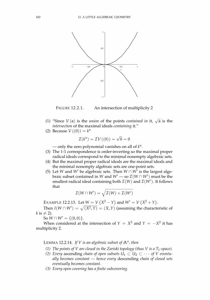
420 12. A LITTLE ALGEBRAIC GEOMETRY
FIGURE 12.2.1. An intersection of multiplicity 2
(1) “Since V (a) is the union of the points contained in it,√a is the
intersection of the maximal ideals containing it.”(2) Because V ((0)) = kn
I(kn) = IV ((0)) =√
0 = 0
— only the zero polynomial vanishes on all of kn.(3) The 1-1 correspondence is order-inverting so the maximal proper
radical ideals correspond to the minimal nonempty algebraic sets.(4) But the maximal proper radical ideals are the maximal ideals and
the minimal nonempty algebraic sets are one-point sets.(5) Let W and W ′ be algebraic sets. Then W ∩W ′ is the largest alge-
braic subset contained in W and W ′ — so I(W ∩W ′) must be thesmallest radical ideal containing both I(W) and I(W ′). It followsthat
I(W ∩W ′) =√I(W) + I(W ′)
EXAMPLE 12.2.13. Let W = V(X2 −Y
)and W ′ = V
(X2 + Y
).
Then I(W ∩W ′) =√(X2, Y) = (X, Y) (assuming the characteristic of
k is 6= 2).So W ∩W ′ = (0, 0).When considered at the intersection of Y = X2 and Y = −X2 it has
multiplicity 2.
LEMMA 12.2.14. If V is an algebraic subset of An, then(1) The points of V are closed in the Zariski topology (thus V is a T1-space).(2) Every ascending chain of open subsets U1 ⊂ U2 ⊂ · · · of V eventu-
ally becomes constant — hence every descending chain of closed setseventually becomes constant.
(3) Every open covering has a finite subcovering.
12.2. HILBERT’S NULLSTELLENSATZ 421
REMARK. Topological spaces satisfying Condition 2 above are callednoetherian. This is equivalent to:
“Every nonempty set of closed subsets of V has a minimalelement.”
Spaces satisfying condition 3 are called compact (although the Bourbakigroup requires compact spaces to be Hausdorff, so they call such spacesquasicompact).
PROOF. Let (a1, . . . , an) be the algebraic set defined by the ideal(X1 − a1, . . . , Xn − an).
A sequence V1 ⊃ V2 ⊃ . . . gives rise to a sequence of radical idealsI(V1) ⊂ I(V2) ⊂ · · · which must eventually become constant by theo-rem 5.4.4 on page 123.
Let V =⋃
i∈I Ui. If V 6= U1, there exists an i1 ∈ I such that U1 $U1 ∪Ui1 . If V 6= U1 ∪Ui1 , continue this process. By statement 2, this muststop in a finite number of steps.
DEFINITION 12.2.15. A function f : An → Am is a regular mapping if itis of the form
f (X1, . . . Xn) =
F1(X1, . . . , Xn)...
Fm(X1, . . . , Xn)
for F1, . . . , Fm ∈ k[X1, . . . , Xn].
If V ⊂ An and W ⊂ Am are algebraic sets and f : An → Am is a regularmapping such that
f (V) ⊂W
then we call f = f |V: V →W a regular mapping from V to W.
Although the Zariski topology is very coarse — implying that it is dif-ficult for a map to be continuous in this topology — there is an importantclass of continuous maps:
PROPOSITION 12.2.16. If f : V ⊂ An → W ⊂ Am is a regular map ofalgebraic sets, then f is continuous in the Zariski topology.
PROOF. The map, f , is continuous if f−1(K) ⊂ An is a closed set when-ever K ⊂ Am is closed. Let
f (X1, . . . Xn) =
F1(X1, . . . , Xn)...
Fm(X1, . . . , Xn)
A closed set K ⊂ Am, in the Zariski topology, is defined by a finite set ofequations
g1(X1, . . . , Xm) = 0...
gt(X1, . . . , Xm) = 0
422 12. A LITTLE ALGEBRAIC GEOMETRY
where the gi are polynomials. f−1(K) is defined by
g1(F1, . . . , Fm)(X1, . . . , Xn) = 0...
gt(F1, . . . , Fm)(X1, . . . , Xn) = 0
which is a closed set in An.
EXERCISES.
1. if R is a principal ideal domain and x = pn11 · · · p
nkk is a factorization
into primes, show that √(x) = (p1 · · · pk)
2. Show that prime ideals are radical.
3. Show that the strong form of the Nullstellensatz implies the weakform.
4. Give an example of a map f : An → Am that is continuous in theZariski topology but not regular.
5. Suppose f =
f1(X1, . . . , Xn)...
fn(X1, . . . , Xn)
: An → An is a regular map and
Ai,j =∂ fi∂Xj
suppose that z = det Ai,j is never 0. Show that it must be a nonzero con-stant.
The Inverse function theorem in calculus implies that f has a smoothinverse in a neighborhood of every point.
Jacobi’s Conjecture states that such an f has an global inverse that is aregular map.
The only cases that have been proved are when k = C and n = 2. It hasbeen shown that proving it for n = 3 would prove it for all n when k = C
— see [35] as a general reference.
6. Find the irreducible components of the algebraic set X2 − YZ =XZ− Z = 0 in A3.
7. If a = (Y3, X−Y), is X + Y ∈ √a? If so, what power of it is in a?
12.3. THE COORDINATE RING 423
12.3. The coordinate ring
The coordinate ring is one of the central concepts of algebraic geometry— particularly the theory of affine algebraic sets. It is the ring of algebraicfunctions on an algebraic set. and it determines all geometric properties.
DEFINITION 12.3.1. Let V ⊂ An be an algebraic set and let a = I(V).Then the coordinate ring of V is defined by
k[V] = k[X1, . . . , Xn]/a
(where the Xi are indeterminates). It is the ring of polynomial functions ofAn restricted to V (or the algebraic functions on V).
EXAMPLE 12.3.2. Let V ⊂ A2 be the hyperbola defined by XY = 1or XY − 1 = 0. It is easily checked that
√(XY− 1) = (XY − 1) so the
defining ideal is (XY− 1). The coordinate ring is
k[X, Y]/(XY− 1) = k[X, X−1]
the ring of so-called Laurent polynomials.
PROPOSITION 12.3.3. The coordinate ring, k[V], of an algebraic set, V, hasthe following properties:
(1) The points of V are in a 1-1 correspondence with the maximal ideals ofk[V].
(2) The closed sets of V are in a 1-1 correspondence with the radical ideals ofk[V].
(3) If f ∈ k[V] and p ∈ V with corresponding maximal ideal mp, thenthe result of evaluating f at p is the same as the image of f under thecanonical projection
π: k[V]→ k[V]/mp = k
In other words, f (p) = π( f ).
PROOF. Let V ⊂ An be an algebraic set. If
π: k[X1, . . . , Xn]→ k[V]
is the canonical projection, and b ⊂ k[V] is an ideal, then lemma 5.2.9 onpage 114 implies that
b 7→ π−1(b)
is a bijection from the set of ideals of k[V] to the set of ideals of k[X1, . . . , Xn]containing a. Prime, and maximal ideals in k[V] correspond to prime, andmaximal ideals in k[X1, . . . , Xn] containing a. The fact that radical ideals areintersections of maximal ideals (see corollary 12.2.12 on page 419) impliesthat this correspondence respects radical ideals too.
If p = (a1, . . . , , an) ∈ V ⊂ An is a point, the maximal ideal of functionsin k[X1, . . . , Xn] that vanish at p is
P = (X1 − a1, . . . , Xn − an) ⊂ k[X1, . . . , Xn]
and this gives rise to the maximal ideal π(P) ⊂ k[V].Clearly
V(
π−1(b))= V (b) ⊂ V
424 12. A LITTLE ALGEBRAIC GEOMETRY
so b 7→ V (b) is a bijection between the set of radical ideals in k[V] and thealgebraic sets contained within V.
To see that f (p) = π( f ), note that the corresponding statement is truein k[X1, . . . , Xn], i.e., the image of f (X1, . . . , Xn) under the map
g: k[X1, . . . , Xn]→ k[X1, . . . , Xn]/P = k
is just f (a1 . . . , an).Let h: k[X1, . . . , Xn] → k[X1, . . . , Xn]/a = k[V] be the canonical projec-
tion. Then mp = h(P) and the diagram
k[X1, . . . , Xn]h //
g
k[V]
π
k k
commutes by lemma 5.2.10 on page 114.
PROPOSITION 12.3.4. Let V ∈ An and W ∈ Am be algebraic sets and letf : V →W be a regular map. Then f induces a homomorphism
f ∗: k[W]→ k[V]
of coordinate rings (as k-algebras).
PROOF. The fact that f is regular implies
f =
F1...
Fm
for F1, . . . , Fm ∈ k[Y1, . . . , Yn] and these polynomials induce a map
F∗: k[X1, . . . , Xm] → k[Y1, . . . , Yn]
g(X1, . . . , Xm) 7→ g(F1, . . . , Fm)
Since f (V) ⊂ W we must have F∗(I(W)) ⊂ I(V). But this means that F∗
induces a homomorphism of k-algebras
f ∗: k[X1, . . . , Xm]/I(W) = k[W]→ k[Y1, . . . , Yn]/I(V) = k[V]
EXAMPLE 12.3.5. Suppose V ⊂ A2 is the parabola y = x2. Then pro-jection to the x-axis
f : A2 → A1
(x, y) 7→ x
is a regular map. There is also a regular map g: A1 → V
g: A1 → A2
x 7→ (x, x2)
It is interesting that we have a converse to proposition 12.3.4:

12.3. THE COORDINATE RING 425
PROPOSITION 12.3.6. Let V ⊂ An and W ⊂ Am be algebraic sets. Anyhomomorphism of k-algebras
f : k[W]→ k[V]
induces a unique regular map
f : V →W
REMARK. This and proposition 12.3.4 on the preceding page implythat the coordinate ring is a contravariant functor (see definition 10.2.1 onpage 341) from the category of algebraic sets to that of k-algebras.
PROOF. We have a diagram
k[X1, . . . , Xm]
k[Y1, . . . , Yn]
k[X1, . . . , Xm]/I(W) k[y1, . . . , yn]/I(V)
k[W]f
// k[V]
and we can map each Xi ∈ k[X1, . . . , Xm] to k[Y1, . . . , Yn] to make
(12.3.1) k[X1, . . . , Xm]
r // k[Y1, . . . , Yn]
k[X1, . . . , Xm]/I(W) k[Y1, . . . , Yn]/I(V)
k[W]f
// k[V]
commute as a diagram of k-algebras. Suppose r(Xi) = gi(Y1, . . . , Yn). Weclaim that
f =
g1...
gm
: An → Am
is the required regular map. If p = (k1, . . . , kn) ∈ V ⊂ An so
v(p) = 0
for any v ∈ I(V), then w( f (p)) = f (w)(p) = 0 for any w ∈ I(W) implyingthat f (V) ⊂W.
If we replace r in diagram 12.3.1 by a map r′ that still makes it commute,the induced f ′ will differ from f by elements of I(V) so
f |V = f ′|Vimplying that the map f : V →W is unique.
426 12. A LITTLE ALGEBRAIC GEOMETRY
DEFINITION 12.3.7. Let V ⊂ An and W ⊂ Am be algebraic sets. ThenV and W are said to be isomorphic if there exist regular maps
f : V → Wg: W → V
such that f g = 1: W →W and g F = 1: V → V.
REMARK. We may regard isomorphic algebraic sets as equivalent inevery way. Then example 12.3.5 shows that parabola y = x2 ⊂ A2 isisomorphic to A1.
We have proved:
COROLLARY 12.3.8. Algebraic sets V ⊂ An and W ⊂ Am are isomorphicif and only if k[V] and k[W] are isomorphic as k-algebras.
REMARK. This proves the claim made earlier: the coordinate ring de-fines all of the significant geometric properties of an algebraic set, includingits isomorphism class.
We can characterize the kinds of rings that can be coordinate rings ofalgebraic sets:
DEFINITION 12.3.9. Given an algebraically closed field k, an affine k-algebra is defined to be a finitely generated k-algebra that is reduced, i.e.√(0) = (0). If A and B are affine k-algebras, the set of homomorphisms
f : A→ B is denotedhomk−alg(A, B)
REMARK. The requirement that the ring be reduced is equivalent to say-ing that it has no nilpotent elements. This is equivalent to saying that theintersection of its maximal ideals is 0 — see theorem 12.2.8 on page 417.
If k is an algebraically closed field, Hilbert’s Nullstellensatz(theorem 12.2.10 on page 418) implies that affine k-algebras (seedefinition 12.3.9) are Jacobson rings (see definition 5.7.2 on page 154).
EXERCISES.
1. Suppose the characteristic of the field k is 6= 2 and V is an algebraicset in A3 defined by the equations
X2 + Y2 + Z2 = 0
X2 −Y2 − Z2 + 1 = 0
Decompose V into its irreducible components.
2. Prove that the statements:a. X is connected if and only if the only subsets of X that are open
and closed are ∅ and X,b. X is connected if, whenever X = X1 ∪ X2 with X1, X2 closed
nonempty subsets of X, then X1 ∩ X2 6= ∅.

12.3. THE COORDINATE RING 427
are equivalent.

CHAPTER 13
Cohomology
“About a thousand years ago, the proof of Pythagoras’s theoremwas thought to be difficult and abstract and suited only for the‘scholastic’ geometers. Today the same theorem is considered anintrinsic component of school education. Perhaps one day alge-bra, sheaf theory and cohomology will be so well understood thatwe will be able to explain the proof of Wiles’ theorem to schoolchildren as well.”
— Kapil Hari Paranjape, essay, On Learning from Arnold’s talkon the Teaching of Mathematics.
13.1. Chain complexes and cohomology
Homology theory is one of the pillars of algebraic topology and a vari-ant called sheaf cohomology is widely used in algebraic geometry. The firststep to developing this theory involves defining cochain complexes — apurely algebraic construct that will be coupled to geometry later.
We will assume all objects here are in a fixed abelian category (see sec-tion 10.5 on page 357), A . For instance, they could be abelian groups ormodules over any ring, or even certain types of sheaves.
We begin with the most basic construct:
DEFINITION 13.1.1. A chain complex (Ci, ∂i) is a sequence of objects ofA and homomorphisms
· · · → Ci+1∂i+1−−→ Ci
∂i−→ Ci−1 −→ · · ·where, for all i, ∂i ∂i+1 = 0. A morphism of cochain complexes fi: (Ci, ∂i)→ (Di, ∂′i) (or chain-map) is a sequence of homomorphisms
fi: Ci → Di
such that the diagrams
(13.1.1) Cifi
//
∂i
Di
∂′i
Ci−1 fi−1
// Di−1
commute for all i. The maps, ∂i, are called the boundary maps or differentialsof the chain-complex. The category of chain-complexes with chain-maps asmorphisms is denoted C h.
429
430 13. COHOMOLOGY
REMARK. The condition ∂i−1 ∂i = 0 implies that im ∂i ⊆ ker ∂i−1. Inalgebraic topology, chain-complexes are geometrically defined objects thatcontain a great deal of topological information.
Now we define a dual concept that is very similar:
DEFINITION 13.1.2. A cochain complex (Ci, δi) is a sequence of objects ofA and homomorphisms
· · · → Ci−1 δi−1−−→ Ci δi−→ Ci+1 → · · ·where, for all i, δi+1 δi = 0. A morphism of cochain complexes fi: (Ci, δi)→ (Di, δ′i) (or chain-map) is a sequence of homomorphisms
fi: Ci → Di
such that the diagrams
(13.1.2) Ci+1 fi+1// Di+1
Cifi
//
δi
OO
Di
δ′i
OO
commute for all i. The maps, δi, are called the coboundary maps or codiff-erentials of the cochain-complex. The category of cochain-complexes withchain-maps as morphisms is denoted Co.
REMARK. The superscripts are not exponents! At this point, thereader may wonder what essential difference exists between chaincomplexes and cochain complexes. The answer is “none!” We can definecochain-complexes as chain-complexes with negative subscripts:
Ci = C−i
(or equivalently, defining chain-complexes as cochain-complexes with neg-ative superscripts). Anything we can prove for one is valid for the otherunder this equivalence.
Historically, chain-complexes appeared first and were geometricallydefined. The generators of the Ci were i-dimensional building blocks for atopological space and the ∂i mapped one of these to its boundary. Cochaincomplexes appeared later as sets of functions one could define on thesebuilding blocks.
In actual applications (in the next section), this symmetry will breakdown to some extent and they both will express complementary informa-tion. We will give greater emphasis to cochain complexes because they arethe ones that are most significant in algebraic geometry.
The condition δi+1 δi = 0 implies that im δi ⊆ ker δi+1 for all i. Withthis in mind, we can define
DEFINITION 13.1.3. Given: a chain-complex, (Ci, ∂i), we can define its homology groups, Hi(C)
viaHi(C) =
ker ∂iim ∂i+1
13.1. CHAIN COMPLEXES AND COHOMOLOGY 431
a cochain complex (Ci, δi), we can define its associated cohomologygroups, Hi(C), via
Hi(C) =ker δi
im δi−1
REMARK. These will also be objects in the category A . If Hi(C) =0, then the original chain complex was an exact sequence. Such chain-complexes are said to be exact or acyclic. A similar definition exists forcochain complexes.
Historically, Hi(C) measured the number of i-dimensional “holes” atopological space had (so an n-sphere has Hn = Z and Hi = 0 for 0 < i <n).
Note that the diagrams 13.1.2 on the preceding page imply that chainmaps preserve images and kernels of the boundary or coboundary homo-morphisms. This implies that
PROPOSITION 13.1.4. A chain map or morphism: of chain complexes fi: (Ci, ∂i)→ (Di, ∂′i) induces homomorphisms of
homologyf i∗: Hi(C)→ Hi(D)
or of cochain-complexes fi: (Ci, δi) → (Di, δ′i) induces homomorphisms
of cohomology groups
f ∗i Hi(C)→ Hi(D)
Next, we consider a property of chain maps:
DEFINITION 13.1.5. Two chain maps f , g: (C, ∂C) → (D, ∂D) of chain-complexes are said to
be chain-homotopic if there exists a set of homomorphisms
Φi: Ci → Di+1
for all i > 0 called a homotopy, such that
fi − gi = Φi−1 ∂C + ∂D Φi
chain maps f , g: (C, δC) → (D, δD) of cochain-complexes are saidto be chain-homotopic if there exists a set of homomorphisms
Φi: Ci → Di−1
called a cohomotopy for all i > 0, such that
fi − gi = Φi+1 δC + δD Φi
REMARK. Chain-homotopy clearly defines an equivalence relation onchain-maps. Although the definition seems odd, the maps Φ arise naturallyin certain topological settings.
The main significance of chain-homotopy is that:
PROPOSITION 13.1.6. If f , g: (C, δC) → (D, δD) are chain-homotopicchain-maps of cochain complexes then
f ∗ = g∗: Hi(C)→ Hi(D)
432 13. COHOMOLOGY
REMARK. A corresponding result exists for chain-complexes, by “re-versing all the arrows.” The symmetry between chain and cochain com-plexes persists.
PROOF. If x ∈ Hi(C), then there exists an element y ∈ ker(δC)i ⊂ Ci
such that x ≡ y (mod im (δC)i−1). If we evaluate ( f − g)(y), we get
( f − g)(y) = (Φ δC + δD Φ) (y)
= δD Φ(y) because y ∈ ker(δC)i
It follows that f (y) ≡ g(y) (mod im (δD)i) and f ∗(x) = g∗(x) ∈ Hi(D).
We can also define an equivalence relation on cochain-complexes:
DEFINITION 13.1.7. Two cochain-complexes (C, δC) and (D, δD) arechain-homotopy equivalent if there exist chain maps
f : (C, δC) → (D, δD)
g: (D, δD) → (C, δC)
such that f g: (D, δD) → (D, δD) and g f : (C, δC) → (C, δC) are bothchain-homotopic to their respective identity maps.
REMARK. Clearly, homotopy equivalent cochain-complexes have iso-morphic cohomology groups
Hi(C) ∼= Hi(D)
for all i. Chain-homotopy equivalence is a much sharper relationship thansimply having isomorphic cohomology groups. In a certain sense, (C, δC)and (D, δD) may be regarded as equivalent in every important respect.
Our final topic in the basic algebra of chain-complexes is:
DEFINITION 13.1.8. If (C, δC), (D, δD), and (E, δE) are cochain com-plexes, an exact sequence
0→ (C, δC)f−→ (D, δD)
g−→ (E, δE)→ 0
are chain-maps f , g such that
0→ Ci fi−→ Di gi−→ Ei → 0
are exact for all i.
REMARK. Exact sequences of cochain complexes arise in many naturalsettings and can be used to compute cohomology because of the next result:
PROPOSITION 13.1.9. An exact sequence
0→ (C, δC)f−→ (D, δD)
g−→ (E, δE)→ 0
of cochain-complexes induces a homomorphism
c: Hi(E)→ Hi+1(C)
13.1. CHAIN COMPLEXES AND COHOMOLOGY 433
for all i, called the connecting map, that fits into a long exact sequence in cohomol-ogy:
· · · → Hi(C)f ∗−→ Hi(D)
g∗−→ Hi(E) c−→ Hi+1(C)→ · · ·Here f ∗ and g∗ are the induced maps and c: Hi(E) → Hi+1(C), called the
connecting map is defined as
c = f−1 δD g−1
or in more detail by(1) If x ∈ Hi(E), then there exists y ∈ ker(δC)i such that x ≡ y
(mod im (δC)i−1).(2) Since g: Di → Ei is surjective, there exists z ∈ Di with g(z) = y.(3) Now take (δD)i(z) = w ∈ Di+1. Since y ∈ ker(δC)i and chain-maps
commute with coboundaries, w ∈ ker g.(4) Since the sequence is exact, this w is in the image of (the injective map)
f so we may regard w ∈ Ci+1.(5) This w ∈ ker(δC)i+1 because it is in the image of δC and its image in D
is in ker(δD)i+1 since (δD)i+1 (δD)i = 0.
REMARK. This will turn out to be very useful for computing cohomol-ogy groups.
PROOF. The proof follows by analyzing the commutative diagram
......
...
0 // Ci+1
(δC)i+1
OO
f// Di+1 g
//
(δD)i+1
OO
Ei+1
(δE)i+1
OO
// 0
0 // Ci
(δC)i
OO
f// Di
(δD)i
OO
g// Ei
(δE)i
OO
//
g−1
f−1ks
0
0 // Ci−1
(δC)i−1
OO
f// Di−1
(δD)i−1
OO
g// Ei−1
(δE)i−1
OO
// 0
...
OO
...
OO
...
OO
in a visual process affectionately (or angrily!) called a “diagram chase”.We show that c is well-defined: any two distinct lifts of y to Di will
differ by an element of Ci. Since the right square commutes, the final re-sult will differ by an element of (δC)
i, hence define the same element ofHi+1(C). If y, y′ both represent the same x, they will differ by an element of(δC)i−1 and their lifts to Di will differ by an element of (δD)i−1, which willbe annihilated when we plug it into (δD)i.
The proof of the remaining assertions (about the sequence being exact)follows by similar arguments and is left to the reader.
If we define Ci = C−i and Hi(C) = H−i(C), we immediately get thecorresponding result for exact sequences of chain-complexes:
434 13. COHOMOLOGY
PROPOSITION 13.1.10. Given a short exact sequence of chain-complexes
0→ (C, ∂C)f−→ (D, ∂D)
g−→ (E, ∂E)→ 0
of chain-complexes, there exists a homomorphism
c: Hi(E)→ Hi−1(C)
for all i, called the connecting map, that fits into a long exact sequence in cohomol-ogy:
· · · → Hi(C)f ∗−→ Hi(D)
g∗−→ Hi(E) c−→ Hi−1(C)→ · · ·We also need two more basic concepts:
DEFINITION 13.1.11. Given a chain-map of cochain complexes
f : (C, δC)→ (D, δD)
the algebraic mapping cone of f is a cochain complex defined by
A( f )n = Cn+1 ⊕ Dn
with a differential
δnA =
[−δn+1
C 0f n+1 δn
D
]:[
Cn+1
Dn
]= A( f )n →
[Cn+2
Dn+1
]= A( f )n+1
and giving a short exact sequence of cochain complexes
(13.1.3) 0→ D → A( f )→ C[+1]→ 0
where C[+1] is C shifted upwards by one degree so C[+1]n = Cn+1 withδn
C[+1] = −δn+1C .
REMARK. It is left as an exercise to the reader to verify that δ2A = 0.
As the name hints, this was originally an algebraic version of a geometricconstruction.
The short exact sequence in 13.1.3 induces a long exact sequence incohomology (proposition 13.1.9 on page 432):
· · · → Hi(D)→ Hi(A( f ))→ Hi(C[+1])→ Hi+1(D)→ · · ·with Hi(C[+1]) = Hi+1(C). Analysis of the connecting map Hi(C[+1])→Hi+1(D) shows that is identical to the map in cohomology induced by f sowe can rewrite the long exact sequence as
(13.1.4) · · · → Hi(C)f ∗−→ Hi(D)→ Hi(A( f ))
→ Hi+1(C)f ∗−→ Hi+1(D)→ · · ·
13.1.1. “Topological” homology and cohomology. In this section, wewill give a crude and (very!) non-rigorous overview of how homology andcohomology were originally developed and what they “mean” — see [51]for rigor and more details.
One way of studying topological spaces involved breaking them upinto a union of discrete pieces of every dimension, called simplices1, and a
1Simplices are essentially polyhedral pieces of Euclidean space. Singular homology andcohomology involves mappings of simplices into a space.
13.1. CHAIN COMPLEXES AND COHOMOLOGY 435
chain-complex was constructed from these simplices. The boundary oper-ator actually represented taking the boundary of n-dimensional simplicesand expressing them as n− 1-dimensional simplices. Although the chain-complex one gets from this construction is not unique (far from it!), it canbe proved that its homology is.
In dimension 0, H0(X; C) = Ck where k is the number of componentsof X. Higher dimensional homology encodes the number of d-dimensional“holes” a space has. For instance, if Sn is an n-sphere, then Hi(Sn; C) = 0for 0 < i < n and Hn(Sn; C) = C.
Cohomology originally studied the behavior of functions on a topolog-ical space — Ci was the set of functions on i-dimensional simplices andthe coboundary operator δi: Ci → Ci+1 determined a function on i + 1-dimensional simplices by taking its value on the boundary. For instanceH0(X; C) is the set of locally-constant functions on X. If X has k compo-nents, this is Ck.
In higher dimensions, Hi(X; C) measures the extent to which certainfunctions on simplices are determined by their behavior on the onthe boundaries of those simplices. Roughly speaking, H1(R2; C) = 0is equivalent to Green’s Theorem in multivariate calculus, andH2(R3; C) = 0 is equivalent to the Divergence Theorem.
EXERCISES.
1. If
0→ (C, δC)f−→ (D, δD)
g−→ (E, δE)→ 0
is an exact sequence of cochain complexes, and two out of the three com-plexes are acyclic, show that the third must be acyclic also.
2. If
0→ (C, δC)f−→ (D, δD)
g−→ (E, δE)→ 0
is an exact sequence of cochain-complexes and D is acyclic, show that
Hi(E) ∼= Hi+1(C)
for all i.
3. Show that, if two chain-maps f , g: (C, δC) → (D, δD) arechain-homotopic and F: A → A ′ is any additive functor (for instance,homA (M, ∗) for any M ∈ A ), then the induced chain-maps
F( f ), F(G): (F(Ci), F(δC))→ (F(Di), F(δD))
are also chain-homotopic. It follows that, if (C, δC) and (D, δD) are chain-homotopy equivalent, then (F(Ci), F(δC)) and (F(Di), F(δD)) also are.
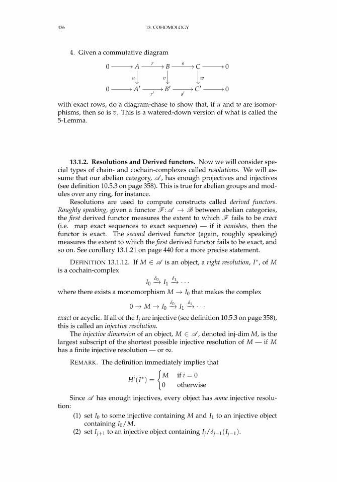
436 13. COHOMOLOGY
4. Given a commutative diagram
0 // A
u
r // B
v
s // C
w
// 0
0 // A′r′// B′
s′// C′ // 0
with exact rows, do a diagram-chase to show that, if u and w are isomor-phisms, then so is v. This is a watered-down version of what is called the5-Lemma.
13.1.2. Resolutions and Derived functors. Now we will consider spe-cial types of chain- and cochain-complexes called resolutions. We will as-sume that our abelian category, A , has enough projectives and injectives(see definition 10.5.3 on page 358). This is true for abelian groups and mod-ules over any ring, for instance.
Resolutions are used to compute constructs called derived functors.Roughly speaking, given a functor F : A → B between abelian categories,the first derived functor measures the extent to which F fails to be exact(i.e. map exact sequences to exact sequence) — if it vanishes, then thefunctor is exact. The second derived functor (again, roughly speaking)measures the extent to which the first derived functor fails to be exact, andso on. See corollary 13.1.21 on page 440 for a more precise statement.
DEFINITION 13.1.12. If M ∈ A is an object, a right resolution, I∗, of Mis a cochain-complex
I0δ0−→ I1
δ1−→ · · ·where there exists a monomorphism M→ I0 that makes the complex
0→ M→ I0δ0−→ I1
δ1−→ · · ·exact or acyclic. If all of the Ij are injective (see definition 10.5.3 on page 358),this is called an injective resolution.
The injective dimension of an object, M ∈ A , denoted inj-dim M, is thelargest subscript of the shortest possible injective resolution of M — if Mhas a finite injective resolution — or ∞.
REMARK. The definition immediately implies that
Hi(I∗) =
M if i = 00 otherwise
Since A has enough injectives, every object has some injective resolu-tion:
(1) set I0 to some injective containing M and I1 to an injective objectcontaining I0/M.
(2) set Ij+1 to an injective object containing Ij/δj−1(Ij−1).
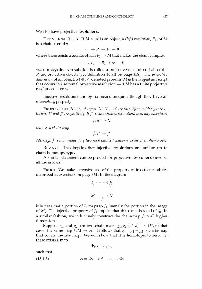
13.1. CHAIN COMPLEXES AND COHOMOLOGY 437
We also have projective resolutions:
DEFINITION 13.1.13. If M ∈ A is an object, a (left) resolution, P∗, of Mis a chain-complex
· · · → P1 → P0 → 0
where there exists a epimorphism P0 → M that makes the chain complex
· · · → P1 → P0 → M→ 0
exact or acyclic. A resolution is called a projective resolution if all of thePi are projective objects (see definition 10.5.2 on page 358). The projectivedimension of an object, M ∈ A , denoted proj-dim M is the largest subscriptthat occurs in a minimal projective resolution — if M has a finite projectiveresolution — or ∞.
Injective resolutions are by no means unique although they have aninteresting property:
PROPOSITION 13.1.14. Suppose M, N ∈ A are two objects with right reso-lutions I∗ and J∗, respectively. If J∗ is an injective resolution, then any morphism
f : M→ N
induces a chain-mapf : I∗ → J∗
Although f is not unique, any two such induced chain-maps are chain-homotopic.
REMARK. This implies that injective resolutions are unique up tochain-homotopy type.
A similar statement can be proved for projective resolutions (reverseall the arrows!).
PROOF. We make extensive use of the property of injective modulesdescribed in exercise 3 on page 361. In the diagram
I0 // J0
M?
OO
f// N?
OO
it is clear that a portion of I0 maps to J0 (namely the portion in the imageof M). The injective property of J0 implies that this extends to all of I0. Ina similar fashion, we inductively construct the chain-map f in all higherdimensions.
Suppose g1 and g2 are two chain-maps g1, g2: (I∗, δ) → (J∗, σ) thatcover the same map f : M → N. It follows that g = g1 − g2 is chain-mapthat covers the zero map. We will show that it is homotopic to zero, i.e.there exists a map
Φi: Ii → Ji−1
such that
(13.1.5) gi = Φi+1 δi + σi−1 Φi
438 13. COHOMOLOGY
Since M maps to 0, we have that g0: I0 → J0 maps the kernel of δ0 to 0,which means that it maps im δ0 ⊂ I1 to J0. The injective property of J1implies that this extends to all of I1, giving
Φ1: I1 → J0
with g0 = Φ1 δ0. Suppose equation 13.1.5 on the previous page is true fordegrees < t. In degree t, consider
gt − σt−1 Φt: It → Jt
(gt − σt−1 Φt) δt−1 = gt δt−1 − σt−1 Φt δt−1
= σt−1 gt−1 − σt−1 Φt δt−1
= σt−1 Φt δt−1 + σt−1 σi−2 Φi−1
−σt−1 Φt δt−1
= σt−1 Φt δt−1 − σt−1 Φt δt−1
= 0
So (gt − σt−1 Φt)|im δt−1 = 0 which means that (gt − σt−1 Φt)| ker δt =0. The argument used above implies that gt − σt−1 Φt defines a mapΦt+1: It+1 → Jt such that
gt − σt−1 Φt = Φt+1 δt
The conclusion follows.
Reversing the arrows proves the chain-complex version
PROPOSITION 13.1.15. Suppose M, N ∈ A are two objects with left resolu-tions P∗ and Q∗, respectively. If P∗ is a projective resolution, then any morphism
f : M→ N
induces a chain-mapf : P∗ → Q∗
Although f is not unique, any two such induced chain-maps are chain-homotopic.
REMARK. This implies that projective resolutions are unique up tochain-homotopy type.
We will be interested in functors F: A → A ′ to other abelian categories:
DEFINITION 13.1.16. A functor F: A → A ′ is left-exact if an exact se-quence
(13.1.6) 0→ A r−→ B s−→ C → 0
in A implies that the sequence
0→ F(A)F(r)−−→ F(B)
F(s)−−→ F(C)
is exact. The functor, F: A → A ′, is right-exact if the sequence 13.1.6 impliesthe exactness of
F(A)F(r)−−→ F(B)
F(s)−−→ F(C)→ 0
REMARK. Exercise 4 on page 361 shows that homA (A, ∗) is left-exact.
13.1. CHAIN COMPLEXES AND COHOMOLOGY 439
PROPOSITION 13.1.17. For a module M over a ring, R, the functor ∗ ⊗R Mis right exact. In other words, the exact sequence
0→ A r−→ B s−→ C → 0
induces an exact sequence
A⊗R M→ B⊗R M→ C⊗R M→ 0
PROOF. Part of this has already been proved in Proposition 10.6.14 onpage 367.
The rest follows from the left-exactness of Hom and proposition 10.6.10on page 365. The exact sequence in 13.1.6 on the facing page induces theexact sequence
0→ HomR(C, homR(M, D))→ HomR(B, homR(M, D))
→ HomR(A, homR(M, D))
which, by proposition 10.6.10 on page 365, is isomorphic to
0→ HomR(C⊗R M, D)→ HomR(B⊗R M, D)
→ HomR(A⊗R M, D)
for an arbitrary module D. This implies
A⊗R M→ B⊗R M→ C⊗R M→ 0
is exact (the details are left to the reader as an exercise).
Since injective resolutions are unique up to chain-homotopy type, thesolution to exercise 3 on page 435 that the following constructs will be well-defined:
DEFINITION 13.1.18. If F: A → A ′ is a left-exact functor and C ∈ Ahas an injective resolution I0 → · · · , then the right derived functors of F are
RiF(C) = Hi(F(I∗)) ∈ A ′
for i ≥ 0.
REMARK. It is not hard to see that R0FC = C. The RiF(C) for i > 0essentially measure how much F fails to be right-exact.
DEFINITION 13.1.19. If M, N ∈ A and I∗ is an injective resolution ofN, the cohomology groups (in A b)
ExtiR(M, N) = Hi(homA (M, I))
depend only on M and N and are functorial.
REMARK. Note that we use hom here rather than Hom. The latteris used for morphisms of modules over a ring, whereas hom is used formorphisms in a category (so it is more general than Hom), in this case A .
Exercise 14 on page 442 shows that we could’ve used a projective reso-lution, P∗, of M to compute Exti
R(M, N):
ExtiR(M, N) = Hi(homA (P∗, N))
440 13. COHOMOLOGY
To analyze the behavior of derived functors, we need the followingresult
LEMMA 13.1.20 (Injective Horseshoe Lemma). Suppose
0→ A r−→ B s−→ C → 0
is a short exact sequence in A and I∗ and J∗ are injective resolutions of A andC, respectively. Then there exists an injective resolution W∗ of B fitting into acommutative diagram
0 // A
εA
r // B
εB
s // C
εC
// 0
0 // I∗ u // W∗ v // J∗ // 0
where the bottom row is a short exact sequence of chain-complexes.
PROOF. Clearly, Wn = In ⊕ Jn for all n. The map εA: A → I0 showsthat a sub-object of B maps to I0. Injectivity implies that this map extendsto all of B, so we get ι: B→ I0 and can define
εB = ι⊕ εC s: B→ I0 ⊕ J0 = W0
We claim that this is injective: if b ∈ B maps to zero, it must map to zeroin J0 so that s(b) = 0. This means that b ∈ im A which maps to I0 via theinjective map, εA.
Suppose this exact sequence of resolutions has been constructed up todegree n so we have
0 // In/im δA
δnA
r // Wn/im δB
f
s // Jn/im δC
δnC
// 0
0 // In+1 u // Wn+1 v // Jn+1 // 0
where the vertical maps are inclusions. Now construct f exactly the way εBwas constructed above.
This immediately implies that
COROLLARY 13.1.21. If
0→ A r−→ B s−→ C → 0
is a short exact sequence in A , and F: A → A ′ is a left-exact additive functor,there exists a natural long exact sequence
0→ F(A)→ F(B)→ F(C)→ R1F(A)→· · · → RiF(A)→ RiF(B)→ RiF(C)→ Ri+1F(A)→ · · ·
REMARK. This long exact sequence is often useful for computing theRiF(A). For instance, if R1F(A) = 0 then the sequence
0→ F(A)→ F(B)→ F(C)→ 0
is exact. If R1F(∗) is always 0, then F is an exact functor.Here is an application:
13.1. CHAIN COMPLEXES AND COHOMOLOGY 441
DEFINITION 13.1.22. If F: A → A ′ is a left-exact additive functor, anobject M ∈ A is called F-acyclic if
RiF(M) = 0
for i > 0.
The long exact sequence in corollary 13.1.21 on the facing page impliesthat
COROLLARY 13.1.23. Let F: A → A ′ be a left-exact additive functor, andlet M be injective or F-acyclic. Then
(1) If0→ A→ M→ B→ 0
is a short exact sequence in A , then
RiF(A) ∼= Ri−1F(B)
for i > 1 and R1F(A) is coker F(M)→ R(B).(2) if
0→ A→ M0 → · · · → Mn−1 → B→ 0with the Mi injective or F-acyclic then
RiF(A) ∼= Ri−nR(B)
and RnF(A) is coker F(Mn−1)→ F(B).(3) If
0→ A→ M0 → · · ·is a resolution by F-acyclic objects, then RiF(A) = Hi(F(M)).
PROOF. To prove the first statement, note that the long exact sequencein corollary 13.1.21 on the preceding page reduces to
0→ F(A)→ F(M)→ F(B)→ R1F(A)→ 0
and0→ RnF(B) δ−→ Rn+1F(A)→ 0
for all n > 0. The second statement follows from the first applied to shortexact sequences
0→ A→M0 → K1 → 00→ Ki →Mi → Ki+1 → 0
0→ Kn−1 →Mn−1 → B→ 0
and induction on n.To prove the third statement, note that we can truncate the resolution
by F-acyclic objects at any point to get
0→ A→ M0 → · · · → Mn−1 → ker δn → 0
and
RnF(A) = coker F(δn−1): F(Mn−1)→ F(ker δn) = ker F(δn) = Hn(F(M))
where F(ker δn) = ker F(δn) is due to the left-exactness of F.
442 13. COHOMOLOGY
EXERCISES.
5. Fill in the details of the proof of proposition 10.6.14 on page 367: If
0→ homR(C⊗R M, D)hom(β⊗1,1)−−−−−−−→ homR(B⊗R M, D)
hom(α⊗1,1)−−−−−−→ homR(A⊗R M, D)
is exact for an arbitrary module, D, then
A⊗R M α⊗1−−→ B⊗R Mβ⊗1−−→ C⊗R M→ 0
is exact.
6. If A ∈ A b is a finite abelian group, show that there is an (unnatural!)isomorphism
A ∼= homA b(A, Q/Z)
and that Ext1Z(A, Z) = A.
7. Show that Q is an injective object in the category of abelian groups.
8. Show that ExtiR(A⊕ B, C) = Exti
R(A, C)⊕ ExtiR(B, C)
9. Show that ExtiR
(⊕j Aj, C
)= ∏j Exti
R(Aj, C)⊕ ExtiR(B, C)
10. Show that ExtiR(lim−→ Aj, C) = lim←− Exti
R(Aj, C)
11. If N is an injective object of A , show that
ExtiR(M, N) = 0
for i > 0 and any object M ∈ A . Conclude that hom(∗, N) is an exactfunctor.
12. If A = R-mod, the category of modules over a commutative ring,R, show that
ExtiR(R, M) = 0
for i > 0 and any R-module, M.
13. If A = R-mod, the category of modules over a commutative ring,R, and P is any projective module over M, show that
ExtiR(P, M) = 0
for i > 0 and any R-module, M, so that homR(P, ∗) is an exact functor.
14. Suppose A = R-mod, M and N are R-modules, and
· · · → P1 → P0 → M→ 0
is a projective resolution (see definition 13.1.13 on page 437). Show that
ExtiR(M, N) = Hi(homR(P∗, N))
so projective resolutions could be used to compute the ExtiR-groups.
15. Compute Ext1Z(Zn, Z) using the exact sequence
0→ Z×n−→ Z→ Zn → 0
of Zn.
13.2. RINGS AND MODULES 443
16. Find an injective resolution for Z in A b.
17. If A = A b show that every abelian group, A, has an injectiveresolution that ends in degree 1 — i.e. is of the form
I0 → I1
so that ExtiZ(A, B) = 0 for A, B ∈ A b and i > 1.
18. Prove a projective version of corollary 13.1.22 on page 441:If
0→ U → Pn → · · · → P1 → A→ 0is an exact sequence of modules over a ring, R, with all of the Pi projective,then
ExtiR(U, M) = Exti+n
R (A, M)
if i > 0.
13.2. Rings and modules
Since the category of modules over a ring has enough projectives (justmap a suitable free module to a module) and enough injectives (proposi-tion 10.5.10 on page 360), we can define homology and cohomology-basedfunctors.
Suppose A = MR, the category of modules over a commutative ring,R.
When R is not commutative (for instance, when R = ZG, a group-ringof a nonabelian group), most of these results still go through but becomeslightly more complicated: for instance, we must make a distinction be-tween right-modules and left-modules.
13.2.1. ToriR-functors. In this section, we study the derived functors of
⊗.
DEFINITION 13.2.1. Given a ring, R, and R-modules, M and N, let
· · · → P2 → P1 → P0 → M→ 0
be an R-projective resolution of M and define
ToriR(M, N) = Hi(P∗ ⊗ N)
REMARK. Proposition 13.1.15 on page 438 implies that ToriR(M, N)
does not depend on the resolution used. The right-exactness of ∗ ⊗ N (seeproposition 13.1.17 on page 439) implies that
Tor0R(M, N) = M⊗R N
PROPOSITION 13.2.2. If M is and R-module and
0→ A→ B→ C → 0
is an exact sequence of R-modules, there exist homomorphisms
∂i+1: Tori+1R (C, M)→ Tori
R(A, M)
444 13. COHOMOLOGY
that fit into a long exact sequence
· · · ∂n+1−−→ TornR(A, M)→ Torn
R(B, M)→ TornR(C, M)→ · · ·
∂2−→ Tor1R(A, M)→ Tor1
R(B, M)→ Tor1R(C, M)
∂1−→ A⊗R M→ B⊗R M→ C⊗R M→ 0
REMARK. This implies that Tor1R(C, M) measures how much ∗ ⊗R M
fails to be right-exact.
PROOF. Let P∗ be a projective resolution of M. Since projectivemodules are flat (see proposition 10.6.20 on page 370) and tensor productswith flat modules preserve exact sequences (see proposition 10.6.18 onpage 369), we get an exact sequence of chain-complexes
0→ A⊗R P∗ → B⊗R P∗ → C⊗R P∗ → 0
which induces a long exact sequence in homology — seeproposition 13.1.10 on page 434. This is the conclusion.
EXAMPLE. If r ∈ R is not a zero-divisor the exact sequence
0→ R ×r−→ R→ R/r · R→ 0
induces
0→ Tor1R(R/r · R, M)→ M ×r−→ M→ M/r ·M→ 0
since R⊗R M = M and (R/r · R)⊗R M = M/r ·M. It follows that
Tor1R(R/r · R, M) = m ∈ M|r ·m = 0
i.e., the r-torsion elements of M. That’s the basis of the name ToriR.
13.2.2. Ext1R and extensions. In this section and the next, we will con-
sider properties of the ExtiR-functors in definition 13.1.19 on page 439.
DEFINITION 13.2.3. If A and B are R-modules, an extension of A by B isa short exact sequence
0→ B→ E→ A→ 0
where E is some module. Two such extensions are considered equivalent ifthey fit into a commutative diagram
0 // B r // E1
v
s // A // 0
0 // Br′// E2
s′// A // 0
Exercise 4 on page 435 implies that v is an isomorphism.Regard an extension as equivalent to 0 if it is split, i.e. of the form
0→ B→ B⊕ A→ A→ 0
13.2. RINGS AND MODULES 445
Given an extension, Corollary 13.1.21 on page 440 shows it induces along exact sequence
0→ homA (A, B)→ homA (A, E)→ homA (A, A)δ−→ Ext1
R(A, B)
We will associate the extension to
(13.2.1) δ(1) ∈ Ext1R(A, B)
where 1 ∈ homA (A, A) is the identity map. The fact that the long exactsequence is natural means that an equivalence of extensions gives rise to acommutative diagram
homA (A, E1)
// homA (A, A)δ // Ext1
R(A, B)
homA (A, E2) // homA (A, A)δ// Ext1
R(A, B)
so equivalent extensions give rise to the same element of Ext1R(A, B).
Given x ∈ Ext1R(A, B) and an injective resolution for B, I∗, represent x
by a homomorphism x: A → I1 whose image lies in the kernel of δ1: I1 →I2. This means it is in the image of I0 and this image is isomorphic to I0/B.We get a commutative diagram
0 // B r // E1
v
s // A
x
// 0
0 // Br′// I0
s′// I0/B // 0
where E1 is a pull-back (see exercise 6 on page 341) of
(13.2.2) I0/B Axoo
I0
s′OO
so
E1 = (α, β) ∈ I0 ⊕ A|s′(α) = x(β)and
s: E1 → A
is the composite E1 → I0 ⊕ Ap−→ A. The kernel of s is the pull-back
I0/B 0oo
I0
s′OO
which is isomorphic to B.
446 13. COHOMOLOGY
This induces a diagram
homA (A, E1)
// homA (A, A)
homA (1,x)
δ // Ext1R(A, B) // Ext1
R(A, E1)
homA (A, I0) // homA (A, I0/B)δ
// Ext1R(A, B) // Ext1
R(A, I0)
Since Ext1R(A, I0) = 0, it is clear that the identity map of A maps to x.
The proof that split exact sequences give 0 is left to the reader.Suppose we vary x by a coboundary — i.e. x′ = x+ ∂ f where f : A→ I0
is a homomorphism. In this case, we get an isomorphism of pull-backs
F =
[1 f0 1
]: E1 ⊂ I0 ⊕ A→ E2 ⊂ I0 ⊕ A
that fits into a commutative diagram
0 // B r // E1
F
s // A // 0
0 // Br′// E2
s′// A // 0
It follows that the class of x ∈ Ext1R(A, B) is what is significant.
We summarize this discussion
THEOREM 13.2.4. Given a ring R and modules A and B, let E(A, B) denotethe equivalence classes of extensions of A by B. The process in equation 13.2.1 onthe previous page gives a 1-1 correspondence
E(A, B)↔ Ext1R(A, B)
REMARK. This gives us an interpretation of Ext1R(A, B): it the set of
equivalence classes of extensions of A by B, and is the reason for the nameof the functor.
Suppose A = Zn and B = Z over the ring Z. In this case
0→ Z→ Q→ Q/Z→ 0
is an injective resolution of Z. A homomorphism
xk: Zn → Q/Z
is defined by1 7→ k/n ∈ Q/Z
where0 ≤ k < n
The extension defined by this is the pullback
Q/Z Znxkoo
Q
s′OO
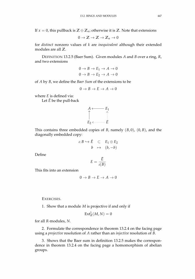
13.2. RINGS AND MODULES 447
If x = 0, this pullback is Z⊕Zn; otherwise it is Z. Note that extensions
0→ Z→ Z→ Zn → 0
for distinct nonzero values of k are inequivalent although their extendedmodules are all Z.
DEFINITION 13.2.5 (Baer Sum). Given modules A and B over a ring, R,and two extensions
0→ B→ E1 → A→ 00→ B→ E2 → A→ 0
of A by B, we define the Baer Sum of the extensions to be
0→ B→ E→ A→ 0
where E is defined via:Let E be the pull-back
A E1oo
E2
OO
E
OO
oo
This contains three embedded copies of B, namely (B, 0), (0, B), and thediagonally embedded copy:
ι: B → E ⊂ E1 ⊕ E2
b 7→ (b,−b)
Define
E =E
ι(B)This fits into an extension
0→ B→ E→ A→ 0
EXERCISES.
1. Show that a module M is projective if and only if
Ext1R(M, N) = 0
for all R-modules, N.
2. Formulate the correspondence in theorem 13.2.4 on the facing pageusing a projective resolution of A rather than an injective resolution of B.
3. Shows that the Baer sum in definition 13.2.5 makes the correspon-dence in theorem 13.2.4 on the facing page a homomorphism of abeliangroups.
448 13. COHOMOLOGY
4. If p is a prime, we know that Ext1Z(Zp, Z) = Zp implying that there
are p inequivalent extensions
0→ Zι−→ M π−→ Zp → 0
and the split extension (M = Z ⊕ Zp) corresponds to 0 ∈ Ext1Z(Zp, Z).
Describe the other p− 1 extensions.
5. Extend exercise 4 to the case
0→ Zι−→ M π−→ Zpq → 0
where p and q are two different primes. Hint: Note that Zpq = Zp ⊕Zqand we have
the split extension
0→ Zι−→ Z⊕Zpq
π−→ Zpq → 0
partially split extensions
0→ Zι−→ Z⊕Zp
π−→ Zpq → 0
0→ Zι−→ Z⊕Zq
π−→ Zpq → 0
and the totally nonsplit extensions
0→ Zι−→ Z
π−→ Zpq → 0
13.2.3. n-fold extensions. We can continue the reasoning in the lastsection to so-called Yoneda extensions.
DEFINITION 13.2.6. If R is a ring and A and B are R-modules, an n-foldextension of A by B is an exact sequence
0→ B→ En → · · · → E1 → A→ 0
Two such extensions
0→ B→ En → · · · → E1 → A→ 0
and0→ B→ E′n → · · · → E′1 → A→ 0
are defined to be equivalent if there exists a commutative diagram
0 // B // En
// · · · // E1
// A // 0
0 // B // E′n // · · · // E′1 // A // 0
It is possible to “standardize” n-fold extensions:
13.2. RINGS AND MODULES 449
LEMMA 13.2.7. Let
· · · → Pn+1 → Pn → · · · → P1 → A→ 0
(note that we are indexing the projective modules in this resolution from 1 ratherthan from 0) be a projective resolution of A. An n-fold extension of A by B isequivalent to one in which n− 1 modules in the extension are projective and of theform:
0 // B // M
// Pn−1
// · · · // P1
// A // 0
0 // B // En // En−1 // · · · // E1 // A // 0
REMARK. The significant thing about this is that most of our “stan-dardized” extension is fixed.
PROOF. Proposition 13.1.15 on page 438 implies that we get a chain-map:
(13.2.3)
· · · // Pn+1
u
v // Pn
q// Pn−1
// · · · // P0
// A // 0
0 // B // En // En−1 // · · · // E1 // A // 0
Given a homomorphism x ∈ hom(Pn, B), we can form the push-out
Pn+1 //
Pn
B // Mor
M =B⊕ Pn
f (Pn+1)
wheref = (u,−v): Pn+1 → B⊕ Pn
We have a homomorphism
ι: B→ M
defined as the composite
B → B⊕ Pn → M
We claim that this is injective. The kernel is given by
ker ι = B⊕ 0∩ im f
Commutativity of
Pn+1
u
v // Pn
pn
B a// En
450 13. COHOMOLOGY
— the leftmost-square of diagram 13.2.3 on the previous page — meansthat v(x) = 0 implies pn v(x) = 0 which implies that a u(x) = 0. Sincea is injective, this means that u(x) = 0 so that ker ι = 0.
We defineM→ Pn−1
to be induced by(0, q): B⊕ Pn → Pn−1
which is well-defined if ker f ⊂ B⊕ ker q. This follows from q v = 0.The map M → En is induced by the defining property of a push-out.
This leads to the result
THEOREM 13.2.8. Let R be a ring and let A and B be R-modules. Thenthe set of equivalence classes of n-fold extensions of A by B is in a one to onecorrespondence with
ExtnR(A, B)
PROOF. Two n-fold extensions are equivalent if and only if their stan-dardized forms
0→ B→ M1 → im Pn → 0and
0→ B→ M2 → im Pn → 0are equivalent. These equivalence classes are in a one-to-one correspon-dence with Ext1
R(im Pn, B). Exercise 18 on page 443 implies that
Ext1R(im Pn, B) = Extn
R(A, B)
and the conclusion follows.
EXERCISES.
6. Define a generalization of the Baer sum for n-fold extensions.
13.3. Cohomology of groups
13.3.1. Introduction. The cohomology of groups is a vast subject suit-able for its own book (for instance, the excellent [17]). We will only touchon it here.
If G is a group, we can construct the group-ring, ZG — a ring of formallinear combinations of elements of G. Let G act trivially on Z so that Z is aZG-module and let
· · · → P2 → P1 → P0 → Z→ 0be a projective resolution of Z.
13.3. COHOMOLOGY OF GROUPS 451
DEFINITION 13.3.1. If A is a left ZG-module define
Hi(G, A) = Hi(homZG(P∗, A)) = ExtiZG(Z, A)
REMARK. In a few cases, it’s easy to say what these groups are:
H0(G, A) = homZG(Z, A) = AG
the submodule of A fixed by G — definition 11.1.7 on page 386.
In order to proceed further, we must construct explicit resolutions ofZ.
PROPOSITION 13.3.2. If G = Zn, generated by T then
ZG = Z[T]/(Tn − 1)
a quotient of a polynomial ring and
Z =ZG
(T − 1)
If x ∈ ZG has the property that (T − 1) · x = 0, then there exists y ∈ ZG suchthat x = N · y where
N = 1 + T + T2 + · · ·+ Tn−1
It follows that
· · · → ZG·(T−1)−−−−→ ZG ·N−→ ZG
·(T−1)−−−−→ ZG → Z→ 0
is a free ZG-resolution of Z.
REMARK. Note that this resolution is periodic so that, if A is a ZG-module with trivial G-action:
H0(G, A) ∼= A
andH2i(G, A) ∼= A/n · A
where i ≥ 1, and
H2i−1(G, A) ∼= H1(G, A) = A[n]
the n-torsion subgroup (see definition 4.6.23 on page 71).
PROOF. The statement that
Z =ZG
(T − 1)
is clear. If (T − 1) · x = 0, and x = ∑n−1i=0 aiTi, then
(T − 1) · x =n−1
∑i=0
(a(i+1) mod n − ai)Ti
so (T − 1) · x = 0 implies that all of the coefficients are the same — i.e.,x = N · a0.
452 13. COHOMOLOGY
The definition of cohomology groups immediately implies that:If G = Zn, then
H1(G, A) =ker(N·: A→ A)
(T − 1) · AFrom this, we get a cohomological statement of Hilbert’s Theorem 90 (seetheorem 8.8.2 on page 316):
THEOREM 13.3.3 (Hilbert’s Theorem 90). If G = Zn for some integer nand G is the Galois group of a field extension
H
F
thenH1(G, H×) = 1
where H× = H \ 0 is the multiplicative (abelian) group of H, regarded as aZG-module.
REMARK. Note: we haven’t used group cohomology to prove Hilbert’sTheorem 90; we are merely stating it in terms of group-cohomology.
PROOF. If x ∈ A, the statement that N · x = 0 is equivalent (whenwriting the operation multiplicatively) to the statement
x · θ(x) · · · θn−1(x) = 1
where θ generates the Galois group, G. This is equivalent to sayingthe norm of x is 1, by theorem 8.8.1 on page 316. The statement thatH1(G, H×) = 1 means that x = θ(y)y−1 for some y ∈ H — orx = zθ(z)−1, where z = y−1 — which is the statement of theorem 8.8.2 onpage 316.
EXAMPLE 13.3.4. If G = Z, ZG = Z[T, T−1] and
0→ ZG·(T−1)−−−−→ ZG → Z→ 0
is a projective resolution of Z, so(1) H0(Z, A) = AZ, the largest submodule fixed by Z.(2) H1(Z, A) = A/ ((T − 1) · A), the largest quotient fixed by Z.(3) Hi(Z, A) = 0 for i ≥ 2.
In order to proceed further, we need a description of projective resolu-tions for all groups.
DEFINITION 13.3.5. If G is a group, its bar resolution, BG, is a ZG-chaincomplex
· · · → BG3d3−→ BG2
d2−→ BG1d1−→ BG0
ε−→ Z→ 0of free ZG-modules where
(1) The basis for BGn is symbols [g1| · · · |gn] for all elements gi 6= 1 ∈G,
(2) BG0 = ZG · [ ], where [ ] is a symbol that is its only basis element.
13.3. COHOMOLOGY OF GROUPS 453
(3) ε: ZG · [ ]→ Z sends all elements of G to 1 ∈ Z
(4) for i > 0, Pi is the free ZG-module on a basis that consists of allpossible symbols [g1| · · · |gn] where 1 6= gi ∈ G for all i.
(5) dn:BGn → BGn−1 is defined by
dn([g1| · · · |gn]) = g1 · [g2| · · · |gn]
+n−1
∑i=1
(−1)i[g1| · · · |gigi+1| · · · |gn]
· · ·+ (−1)n[g1| · · · |gn−1]
Here, if a term has a 1 in it, we identify it with 0, so
d1([g|g−1]) = g[g−1]− [1] + [g] = g[g−1] + [g]
This is a resolution because it has a contracting homotopy given by
Φi:BGi → BGi+1
g · [g1| · · · |gi] 7→ [g|g1| · · · |gi] if g 6= 11 · [g1| · · · |gi] 7→ 0
for i ≥ 0 andΦ−1(1) = [ ]
such that
(13.3.1) 1− εi = di+1 Φi + Φi−1 di
where εi = 0, if i > 0, and ε0 = ε, as defined above. It follows that the0-map is chain-homotopic to the identity (see definition 13.1.5 on page 431and proposition 13.1.6 on page 431) above dimension 0, and the homologyof this complex must vanish.
REMARK. This was originally defined by Eilenberg and Maclane in [32,33] and MacLane’s book [70]. The term “bar resolution” comes from theiruse of vertical bars rather than ⊗’s because they take up less space2.
This is what is called the normalized bar resolution; it is slightly smallerthan the unnormalized bar resolution, which allow 1’s in the bar-symbols.
EXERCISES.
1. Show that the resolution in definition 13.3.5 on the facing page is achain-complex, i.e., that di di+1 = 0 for all i.
2. Verify equation 13.3.1.
2Typographically!
454 13. COHOMOLOGY
13.3.2. Extensions of groups. In this section we will apply the coho-mology of groups to study the extension problem for groups:
Given two groups H and N, which groups, G, have theproperty that(1) N C G(2) there exists an exact sequence
(13.3.2) 1→ N ι−→ G π−→ H → 1
?Such groups, G, are called extensions of H by N (comparedefinition 13.2.3 on page 444).
This is an extremely difficult problem in general but we know solutions inspecial cases:
If N is abelian and the extension is split — i.e., if there’s a homomorph-ism g: H → G with the property that π g = 1: H → H in 13.3.2, thenexercise 5 on page 80 shows that
G = N oϕ H
the semidirect product.
PROPOSITION 13.3.6. An extension of a group H by an abelian group, N
1→ N ι−→ G π−→ H → 1
defines a ZH-module structure on N by conjugation
ϕ: H → Aut(N)
PROOF. We define a function (not a homomorphism!)
g: H → G
such that π g = 1: H → H. The H-action on N is defined by conjugation
ϕ(h)(n) = g(h) · n · g(n)−1
Note: since N is abelian, varying g(h) by an element of N doesn’t changethe result of conjugation so we actually get a homomorphism
H → Aut(N)
Compare this with 13.2.3 on page 444
DEFINITION 13.3.7. Two extensions, G1and G2 are defined to be equiv-alent if there exists a commutative diagram
1 // Nι1 // G1
π1 //
H // 1
1 // Nι2// G2 π2
// H // 1
13.3. COHOMOLOGY OF GROUPS 455
The results of section 13.2.2 on page 444 suggest that the cohomologyof groups might be useful — at least in the case where N is abelian.
Throughout the remainder of this section N denotes an abelian groupthat is a module over ZH and we will study extensions like
(13.3.3) 1→ N ι−→ G π−→ H → 1
We will consider functions
(13.3.4) g: H → G
such that π g = 1: H → H. Given h1, h2 ∈ H, consider x(h1, h2) =g(h1)g(h2)g(h1h2)
−1and we require g(1) = 1.
DEFINITION 13.3.8. Given a group-extension as in 13.3.3 and a mapg: H → G with the property g(1) = 1, the function
x: H × H → N
defined as x(h1, h2) = g(h1)g(h2)g(h1h2)−1 is called a factor-set for the ex-
tension.
Since the extension in 13.3.3 is not split, g in 13.3.4 is not a homo-morphism so x(h1, h2) 6= 1. Since it maps to 1 in H, we conclude thatx(h1, h2) ∈ N.
If we identify G with N × g(H) (as sets), a factor-set for an extensiondetermines it because
(n1g(h1))(n2g(h2)) = (n1g(h1)n2g(h1)−1g(h1)g(h2))
= (n1 ϕ(h1)(n2)g(h1)g(h2))
= (n1 ϕ(h1)(n2)g(h1)g(h2)g(h1h2)−1g(h1h2))
= (n1 ϕ(h1)(n2) · x(h1, h2)g(h1h2))
or
(13.3.5) (n1, h1)(n2, h2) = (n1 + ϕ(h1)(n2) + x(h1, h2), h1h2)
since the N-group is abelian. Note that, if the factor-set is zero, this becomesthe product-formula for the semidirect product.
PROPOSITION 13.3.9. A function, x: H × H → N, is a factor-set for theextension in 13.3.3 if and only if it defines a 2-cocycle
BH2 → N
with respect to the bar-resolution (see definition 13.3.5 on page 452).
PROOF. This is the same as saying the composite
BH3d3−→ BH2
x−→ N
is zero, i.e.
(13.3.6) ϕ(h1) (x(h2, h3))− x(h1h2, h3) + x(h1, h2h3)− x(h1, h2) = 0
456 13. COHOMOLOGY
If x is a factor-set, this follows from the associativity of the product in equa-tion 13.3.5 on the preceding page:
((0, h1)(0, h2)) (0, h3) = (x(h1, h2) + x(h1h2, h3), h1h2h3)
(0, h1) ((0, h2)(0, h3)) = (ϕ(h1) (x(h2, h3)) + x(h1h2, h3), h1h2h3)
and setting the difference between these to 0 gives equation 13.3.6 on theprevious page.
Conversely, if x is a 2-cocycle, equation 13.3.5 on the preceding pagegives an associative product on N × H and
(n, h)−1 =(−ϕ(h−1)(n)− ϕ(h−1)
(x(h, h−1)
), h−1
)so we can define an extension group from x.
LEMMA 13.3.10. If x1, x2: H× H → N are two factor-sets giving rise to thesame extension
1→ N → E→ H → 1then
x1 − x2
is a coboundary in the bar-resolution of N. It follows that a factor-set correspondsto a well-defined element of
H2(H, N)
PROOF. We will write the group-operation multiplicatively. If the xi areinduced by functions
gi: H → E
then g1(h)g2(h)−1 = θ(h) ∈ N for all h ∈ H, so g1(h) = θ(h) · g2(h).
x1(h1, h2) = g1(h1)g1(h2)g1(h1h2)−1
= θ(h1)g2(h1)θ(h2)g2(h2) [θ(h1h2)g2(h1h2)]−1
= θ(h1)g2(h1)θ(h2)g2(h2)g2(h1h2)−1θ(h1h2)
−1
= θ(h1)g2(h1)θ(h2)g2(h1)−1g2(h1)g2(h2)g2(h1h2)
−1θ(h1h2)−1
= θ(h1)θ(h2)g2(h1)g2(h1)g2(h2)g2(h1h2)
−1θ(h1h2)−1
= θ(h1)θ(h2)g2(h1)x2(h1, h2)θ(h1h2)
−1
Since the equation on the bottom line takes place entirely in the abeliangroup, N, we may write it additively
x1(h1, h2) = θ(h1) + θ(h2)g2(h1) − θ(h1h2) + x2(h1, h2)
or
x1(h1, h2)− x2(h1, h2) = θ(h1) + θ(h2)g2(h1) − θ(h1h2)
= ϕ(h1) (θ(h2))− θ(h1h2) + θ(h1)
= θ (d2 ([h1|h2]))
whered2:BH2 → BH1
13.3. COHOMOLOGY OF GROUPS 457
is the boundary map of the bar-resolution of H (see definition 13.3.5 onpage 452).
Considering definition 13.3.7 on page 454, we conclude that
THEOREM 13.3.11. If H is a group and N is an abelian group with the struc-ture of a ZH-module, the set of equivalence classes of extensions of N by H is in aone-to-one correspondence with elements of
H2(H, N)
The split extension corresponds to 0 ∈ H2(H, N) (the semi-direct product —see 4.7.15 on page 79 and exercise 5 on page 80).
Extensions in which N is not abelian are much more complex and theirstudy involves nonabelian cohomology and algebraic topology. See [18].
EXERCISES.
3. If F is a free group and A is any ZF module, show that
H2(F, A) = 0
4. If F is a free group and A is any ZF module, show that
Hi(F, A) = 0
for all i > 1.

APPENDIX A
Axiomatic Set Theory
“Either mathematics is too big for the human mind or the humanmind is more than a machine.”
— Kurt Gödel.
A.1. Introduction
In this section, we will give a rigorous set of axioms defining set the-ory. The reader might wonder why this is necessary: after all sets are justcollections of stuff.
In the 19th century, sets were regarded as any collection of objects thatcould be described in any terms — and elements of sets could be any objectsthat one could describe.
In [108], the philosopher Bertrand Russell pointed out a problem withthis very loose definition of a set:
Since sets could theoretically be elements of themselves,let S be the set of all sets that do not contain themselvesas an element. The question is: Is S an element of S? Ifthe answer is yes, then S cannot be an element of S. If theanswer is no, then S must be an element of S.
Bertrand Arthur William Russell, 3rd Earl Russell, (1872 – 1970) was aBritish philosopher, logician, mathematician, historian, writer, social criticand political activist. He is well-known for his political leaning towardpacifism, initiating the Russell–Einstein Manifesto opposing the develop-ment of atomic weapons. His main mathematical work is [108].
The result of this is that set theory today is defined in terms of axioms:
A.2. Zermelo-Fraenkel Axioms
We resolve questions like the Russell Paradox via a system of axiomsthat define what we mean by sets. We present an abbreviated version ofthese axioms. In these axioms, symbols like ∈ are boolean-valued opera-tions so, if x is not a set, y ∈ x is false for any y. The axioms describe howwe are allowed to use these symbols in equations1.
1Roughly speaking, concrete “definitions” of these symbols in terms of other objects arecalled models of set theory. In [24], P. Cohen shocked the mathematical world by showing thatmultiple inequivalent models exist for set theory (in one of which all sets are countable).
459
460 A. AXIOMATIC SET THEORY
AXIOM A.2.1 (Extensionality). Two sets are equal (are the same set) if theyhave the same elements:
∀x,y [∀z(z ∈ x ⇔ z ∈ y) =⇒ x = y]
This is straightforward but has to be said.
AXIOM A.2.2 (Regularity). Every nonempty set x contains an element ysuch that x and y are disjoint.
∀x[∃a(a ∈ x) =⇒ ∃y (y ∈ x ∧ ∀z (z ∈ x =⇒ z /∈ y))
]The element y ∈ x with this property is said to be ∈-minimal. This
axiom has a number of interesting consequences:
(1) No set can be a member of itself (preventing the Russell Paradox).Suppose A is a set and consider the set A. The Regularity Ax-iom implies that there exists a y ∈ A that is disjoint from it.Since the only element of A is A, we have y = A and
A ∈ A =⇒ A /∈ y = A
(2) No infinite descending chain of set-containments2 exists. Let f be afunction defined on the natural numbers such that(a) f (n) is a set for all n and(b) f (n + 1) ∈ f (n) for all n
Let S = f (n)|n ∈N. If y ∈ S is any element, y = f (k) for somek and f (k + 1) ∈ y, so f (k + 1) ∈ f (k)∩ S, violating the RegularityAxiom. This only happens for infinite chains — something thatmight crudely be represented by
∞x∞, ∞−1x∞−1, . . .
where one is to imagine an infinite number of brackets enclosingthe x.
Given a finite chain like
x , x , x , xwe have
x ∈ x ∈ x ∈ xand there’s a minimal element (x, in this case) that doesn’t containany of the others.
AXIOM A.2.3 (Specification). Given a set, one can define a subset by impos-ing a condition on its elements. In other words, one is allowed to use constructionslike
x ∈ S|φ(x)to define sets, where φ is some logical function and S is a set.
2In this context “set-containment” means one set is an element of another — not a subset.
A.2. ZERMELO-FRAENKEL AXIOMS 461
This is what is called an axiom schema since there are an infinite numberof possible functions φ and this gives rise to an axiom for each of them.
One consequence of this is that empty sets exist. If x is any set, we candefine a set
y ∈ x|y 6= yand the Axiom of Extensionality implies that any two such sets are equal,so we have a unique empty set, denoted ∅.
AXIOM A.2.4 (Pairing). Given two sets x and y there exists a set, z, thatcontains x and y as elements
∀x,y∃z (x ∈ z ∧ y ∈ z)
AXIOM A.2.5 (Union). The union over the elements of a set exists and is aset.
∀z∃u∀x,y ((x ∈ y) ∧ (y ∈ z)) =⇒ x ∈ u
AXIOM A.2.6 (Replacement). The image of a set under any definable func-tion lies in a set.
This is also an axiom schema since the set of possible functions is infi-nite.
AXIOM A.2.7 (Infinity). There exists a set with infinitely many elements.
∃x[∅ ∈ x ∧
(∀yy ∈ x =⇒ (y ∪ y) ∈ x
)]AXIOM A.2.8 (Power set). Given a set, S, there exists a set whose elements
are all of the subsets of S (where a subset of S is defined as a set whose elements arecontained in S)
AXIOM A.2.9 (Well-ordering). Any set, S, can be well-ordered. This meansthat there exists a binary order-relation, ≺, such that
if x, y ∈ S with x 6= y, then x ≺ y or y ≺ x (but not both), if T ⊂ S is a subset then T has a minimal element — i.e., there exists
x ∈ T such that x ≺ y for all y ∈ T with y 6= x.
REMARK A.2.10. The well-ordering axiom is completely trivial for fi-nite sets.
For infinite sets, it has many subtle ramifications. For instance, if S =Q, the well-ordering cannot possibly be the usual ordering, <, of rationalnumbers because an open interval like (0, 1) has no minimal element. Wecan construct a well-ordering of the positive rationals: If p/q ∈ Q is reduced(i.e. gcd(p, q) = 1), define h(p/q) = |p| + |q| and order the rationals bythis h-function. When two numbers have the same value of h, order themby the denominator. In this ordering, the minimal element of (0, 1), is 1/2.
At the time of this writing, there is no known well-ordering of the realnumbers.
The well-ordering axiom implies another
THEOREM A.2.11 (Axiom of choice). Given a set S and a collection ofnonempty sets indexed by S:Gα, α ∈ S, there exists a function
f : S→ G =⋃
α∈SGα
462 A. AXIOMATIC SET THEORY
that selects an element f (α) ∈ Gα ⊂ G.
REMARK. This is often stated asThe Cartesian product
∏α∈S
Gα
is nonempty.Although this also seems self-evident, it has bizarre implications for infinitefamilies of sets. It is possible to prove the well-ordering axiom from theaxiom of choice and the other axioms of set theory, so the two are equivalent.This proof is beyond the scope of this book.
PROOF. Simply well-order G and define f (α) to be a minimal elementin Gα ⊂ G.
The well-ordering axiom also implies Zorn’s lemma, a classic resultfound in [65, 111]:
LEMMA A.2.12. If S is a partially-ordered set with the property that everyincreasing sequence of elements
e1 e2 · · ·has an least upper bound, then S contains a maximal element (“increasing” meansei 6= ei+1 for all i).
If every decreasing sequence of elements
e1 e2 · · ·has a lower bound, then S has a minimal element.
REMARK. In this context,(1) “least upper bound” means an element f such that f ei for all i
and for any other g ei, f g.(2) “maximal” means “there is an element e ∈ S such that there does
not exist an element e′ ∈ S with e e′ and e′ 6= e.”Zorn’s lemma is equivalent to the axiom of choice and the well-orderingaxiom (which are equivalent to each other) in set theory. Proving all ofthese equivalences is beyond the scope of this book3 — see [55] as a generalreference.
PROOF. We give a non-rigorous proof that can be made rigorous usingtransfinite induction and ordinals. Let P = P(S) \ ∅ and let
S =⋃
A∈PA
Now use the Axiom of Choice ( A.2.11 on the preceding page) to define afunction
f : P→ Swith f (A) = a ∈ A — this just maps every nonempty subset of S to one ofits elements. Define the function
F: I → A ∪ A3We proved the “easy” one in theorem A.2.11 on the previous page.
A.2. ZERMELO-FRAENKEL AXIOMS 463
where I is some ordered collection of indices to be defined later, via
F(α) =
f (s ∈ S|F(β) s, for all β < α) if this set is nonemptyA otherwise
If S is finite and I = Z, then F(n) will be A for some value of n — wewill have constructed an ascending chain that exhausts all of the elements ofS with elements all other elements of S. Since this chain has an upperbound, F(n− 1) will be maximal.
If S is infinite, the idea is basically the same except that I consists ofinfinite ordinals4 — the totality of which is known not to constitute a set.We also need transfinite induction to properly define F. It turns out thatthere exists an ordinal α such that F(α) = A and α = β + 1 and F(β) is themaximal element.
4See [55] as a general reference, again.

APPENDIX B
Further topics in ring theory
“Geometry is one and eternal shining in the mind of God. Thatshare in it accorded to men is one of the reasons that Man is theimage of God.”
— Johannes Kepler, Conversation with the Sidereal Messenger(an open letter to Galileo Galilei), [94].
This appendix deals with topics that are more specialized than thoseconsidered in chapter 5 on page 107. They have applications to AlgebraicGeometry and other areas.
B.1. Discrete valuation rings
In this section we define a class of rings that is important in algebraicgeometry. Their main property is that they have an especially simple ideal-structure.
Krull introduced them with the concept of valuation in his work on al-gebraic number theory in [62]. A valuation on a field is a function that canbe used to define a metric on this field. We have already seen an exampleof this in claim 5.1.8 on page 109 — the function v(x), there, is an exampleof a valuation.
DEFINITION B.1.1. Let F be a field and let F× ⊂ F denote the subset ofnonzero elements. A discrete valuation on F is a surjective function
v: F× → Z
with the properties:(1) v(x · y) = v(x) + v(y) for all x, y ∈ F×
(2) v(x + y) ≥ min(v(x), v(y))
REMARK. Statement 2 implies that v(1) = v(1 · 1) = v(1) + v(1) = 0.If 0 < α < 1 is some real number, it is not hard to see that
αv(∗): F× → [0, 1]
defines a metric on F, where we define the metric of 0 to be 0.
The definition of valuation easily implies the following properties:
PROPOSITION B.1.2. Let F be a field with valuation v: F× → Z. Then(1) v(x−1) = −v(x) for all x ∈ F∗, since v(x · x−1) = v(1) = 0 =
v(x) + v(x−1).(2) v(−1) = 0, because v(1) = v((−1) · (−1)) = v(−1) + v(−1) if the
characteristic of F is 6= 2. If it is 2, then −1 = 1, so the statement stillholds.
465
466 B. FURTHER TOPICS IN RING THEORY
(3) v(−x) = v(x), because −x = x · (−1).(4) if v(x) > v(y) then v(x + y) = v(y). Certainly, it must be ≥ v(y)
but, if we write y = x + y− x, we get v(y) ≥ min(v(x + y), v(x)).
It is easy to find examples of valuations:
EXAMPLE B.1.3. If F = Q and p ∈ Z is any prime then we can definethe p-adic valuation, vp, as follows:
For any q ∈ Q we have a unique representation
q = ∏ pnii
where the pi are primes and ni ∈ Z are integers (which are negative if aprime only occurs in the denominator of q). If p = pj, define
vp(q) = nj
It is well-known that the p-adic valuations constitute all of the discretevaluations on Q — see [61].
If a field, F, has a valuation
v: F× → Z
proposition B.1.2 on the previous page implies that the set of elementsx ∈ F with v(x) ≥ 0 form a ring, i.e., are closed under addition and multi-plication.
Other interesting examples are provided by power-series rings andvariants
EXAMPLE B.1.4. If k is a field, R = k[[X]] is the ring power-series in Xand F = k((X)) is the field of fractions of R, exercise 6 on page 249 impliesthat every element in F can be written uniquely in the form
f = Xα · rwith r ∈ R. It follows that F is a field with valuation given by v( f ) = α.The subring of elements with a valuation ≥ 0 is precisely R ⊂ F.
There are valuations that are not discrete in the sense above:
EXAMPLE B.1.5. We can also define the field of Puiseux series, discov-ered by Isaac Newton in 1676 ([81]) and rediscovered by Victor Puiseux([91]) in 1850:
kX =∞⋃
n=1
k((X1/n))
An argument analogous to that used in the power-series case implies thatevery element of kX can be uniquely written in the form
f = Xq ·(
a0 + a1X1/n + a2X2/n + · · ·)
for some n ∈ Z, n ≥ 1, some q ∈ Q, and a0 6= 0 ∈ k. We can define thevaluation of f to be q.
REMARK. If k is algebraically closed and of characteristic 0, it turns outthat kX is the algebraic closure of k((X)). Newton sketched a proof in aletter he wrote in 1676. See [86] for a short modern proof.
B.1. DISCRETE VALUATION RINGS 467
DEFINITION B.1.6. Let R be an integral domain with field of fractionsF. Then R is a discrete valuation ring if there exists a valuation
v: F× → Z
such thatR = x ∈ F|v(x) ≥ 0
This ring has an ideal
m = x ∈ F|v(x) > 0The notation for a discrete valuation ring is (R,m).
REMARK. The properties of a valuation (in proposition B.1.2 onpage 465) imply that m is an ideal and that all x ∈ R \m are units, so m isthe unique maximal ideal, and R is a local ring.
For the p-adic valuation on Q, the corresponding discrete valuationring is Rp ⊂ Q of fractions whose denominator is relatively prime to p(when it is reduced to the lowest form). The maximal ideal is p · Rp.
As mentioned above, discrete valuation rings have an extremely simpleideal-structure:
LEMMA B.1.7. Let (R,m) be a discrete valuation ring defined by a valuation
v: F× → Z
on the field of fractions, F, of R. Then there exists an element r ∈ R such thatm = (r) and all ideals of R are of the form (rn) for n ∈ Z+.
PROOF. Suppose u ∈ R has v(u) = 0. Then v(u−1) = 0 also, so u isa unit. If I ⊂ R is an ideal, let x ∈ I be the element with the smallestvaluation. If y ∈ I, then x−1y ∈ F has a valuation v(y) − v(x) ≥ 0 sox−1y ∈ R and y = x · x−1y and I = (x), and all ideals are principal. Itfollows that m = (r) and v(r) = 1 (since the valuation-map is surjective).
Suppose y ∈ R has the property that v(y) = n. Then r−ny has valuation0 so it is a unit and (y) = (rn).
It is interesting to determine the properties a general ring must have tobe a discrete valuation ring:
LEMMA B.1.8. Let R be a noetherian local domain with maximal ideal m ∈ Rand suppose that this is the only prime ideal (other than the trivial prime ideal,(0)). Then R is a discrete valuation ring if and only if it is integrally closed in itsfield of fractions.
PROOF. First, we show that a discrete valuation ring is integrallyclosed. If F is the field of fractions of R and x/y ∈ F is integral over R, then
(x/y)n + an−1(x/y)n−1 + · · ·+ a0 = 0
with the ai ∈ R. If v(x) < v(y) then
v((x/y)n + an−1(x/y)n−1 + · · ·+ (x/y)a1) = v(−a0) ≥ 0
Proposition B.1.2 on page 465 implies that
v((x/y)n + an−1(x/y)n−1 + · · ·+ (x/y)a1) = v((x/y)n) < 0
468 B. FURTHER TOPICS IN RING THEORY
which is a contradiction. It follows that v(x) ≥ v(y) and x/y ∈ R.Now we work in the other direction: assume R satisfies the hypotheses
(i.e., it is a noetherian local domain with a unique prime ideal) and showthat it is a discrete valuation ring if it is integrally closed.
For every u ∈ m and v ∈ R \ (u) define
(B.1.1) (u: v) = r ∈ R|rv ∈ (u)
This is easily verified to be an ideal and nonempty (since it contains u atleast). Let (a: b) be the maximal such ideal (with respect to inclusion). Weclaim that it is a prime ideal. If xy ∈ (a: b), then xyb ∈ (a). Note that(a: yb) ⊇ (a: b). If x, y /∈ (a: b), then yb /∈ (a) and x ∈ (a: yb) so (a: yb) )(a: b), which contradicts the maximality of (a: b).
Since m is the only prime ideal of R, we have m = (a: b). We claim thatm = (a/b) (so b|a). Equation B.1.1 for (a: b) implies that (b/a) · (a: b) =(b/a) ·m ⊂ R.
If (b/a) · m 6= R then (b/a) · m must be an ideal of R, hence (b/a) ·m ⊂ m. Since R is noetherian, m must be a finitely generated R-module.Since (b/a) maps a finitely-generated R-module to itself, proposition 6.5.2on page 249 implies that b/a is integral over R, hence in R (because R isintegrally closed). This is a contradiction (by the condition above equa-tion B.1.1), so we conclude that (b/a)m = R and m = R · (a/b) = (a/b).
We claim that all ideals in R are principal. If not, there is a maximalnon-principal ideal I (because R is noetherian). We must have
I ⊂ m = (a/b)
Now consider
I ⊂ (b/a) · I ⊂ (b/a) ·m = R
If I = (b/a) · I, then by the reasoning above and proposition 6.5.2 onpage 249, we conclude that (b/a) is integral over R, hence in R. This isthe same contradiction as before (with m) and we conclude that
I ( (b/a) · I
which implies that the ideal (b/a) · I is principal, say (b/a) · I = (x). Thenwe get I = (x · a/b) which is a contradiction.
We conclude that all ideals are principal, and that R is a unique factor-ization domain by remark 5.3.12 on page 119. The element π = a/b thatdefines m must be irreducible and a prime, so we can define a function
v: R \ 0 → Z
by setting v(x) to the highest power of π that divides x. This extends to avaluation
v: F× → Z
v(x/y) = v(x)− v(y)
and R is a discrete valuation ring.
B.3. GRADED RINGS AND MODULES 469
B.2. Metric rings and completions
Rings with metrics arise naturally in areas of analysis and number the-ory.
We begin by defining a metric space.
DEFINITION B.2.1. A metric space, M, is a set of points equipped witha function, d(x, y) ∈ R, for every x, y ∈ M with the properties
(1) d(x, y) ≥ 0 for all x, y ∈ M and d(x, y) = 0 if and only if x = y(2) d(x, y) = d(y, x) for all x, y ∈ M.(3) Given x, y, z ∈ M, d(x, z) ≤ d(x, y) + d(y, z) (Triangle inequality).
REMARK. It is well-known that Q and R are metric spaces withd(x, y) = |x− y|. We have many more examples of metric rings because:
PROPOSITION B.2.2. If R is a discrete valuation ring with valuationv: F× → Z and α ∈ (0, 1), then v(x, y) defined by d(x, y) = |x− y|, where | ∗ |is defined by
(1) |0| = 0 for all x ∈ R
(2) if x ∈ R, and x 6= 0, then d(x, y) =(
12
)v(x)
is a metric on R.
REMARK. Note that this “absolute value” has the property that |x · y| =|x| · |y|.
PROOF. This follows by the properties of a valuation inproposition B.1.2 on page 465:
DEFINITION B.2.3. An infinite sequence of points, an, in a metricspace approaches a limit a if, for every ε > 0, there exists an integer N(ε)such that
|ai − a| < ε
for all i > N(ε) (where | ∗ | denotes distance). A sequence that has a limitis said to converge.
We need a criterion for a limit to exist. It’s certainly necessary for theterms of the sequence to get arbitrarily close to each other:
DEFINITION B.2.4. An infinite sequence of points in a metric space anis said to be Cauchy if, for every ε > 0, there exists an integer N(ε) such that
|ai − aj| < ε
for all N(ε) < i < j. If every Cauchy sequence in a metric space, M,converges, we say that M is complete.
REMARK. Clearly, any convergent sequence is Cauchy.
B.3. Graded rings and modules
A graded ring is a kind of ring subdivided into distinct directsummands. These appear in the study of projective varieties andsheaf-cohomology.
470 B. FURTHER TOPICS IN RING THEORY
DEFINITION B.3.1. A ring, G, is called a graded ring over k if there existsa decomposition
G = G0 ⊕ G1 ⊕ · · ·such that Gi · Gj ⊂ Gi+j for all i, j ≥ 0. If I ⊂ G is an ideal, we say that I isa graded ideal if
I = I0 ⊕ I1 ⊕ · · ·where Ij = I ∩ Gj for all j ≥ 0. An ideal H ⊂ G is homogeneous if all of itsgenerators come from the same Gn for some n.
REMARK. Any ring, R, can be regarded as a graded ring, if we defineR0 = R, Ri = 0 for i > 0. A polynomial ring, k[X1, . . . , Xt] is naturallygraded with gradation given by the total degree of a monomial (where wehave specified the degree of each of the Xi):
k[X1, . . . , Xt] = k⊕ K1 ⊕ K2 ⊕ · · ·where Kn is the vector space generated by all monomials of total degreen. For instance, let G = k[X, Y] where X and Y are of degree 1 and letH = k[X, Y] where X is of degree 1 and Y is of degree 2. Then:
G0 = kG1 = k · X, YG2 = k · X2, XY, Y2
...
and
H0 = kH1 = k · XH2 = k ·Y
...
so G and H are isomorphic as rings but not as graded rings.Given graded algebras over a ring R, we can define the graded tensor
product
DEFINITION B.3.2. If A, B are graded algebras over a (non-graded)ring, R, the tensor product is the graded algebra A⊗R B defined by
(A⊗R B)n =⊕
i+j=nAi ⊗R Bj
REMARK. This definition is consistent with the convention
(a⊗ b) · (c⊗ d) = (ac⊗ bd)
It is not hard to see that:
PROPOSITION B.3.3. If H ⊂ G is a homogeneous ideal of a graded ring G, itis not hard to see that
(B.3.1)GH
=∞⊕
i=0
Gi +H
H
B.3. GRADED RINGS AND MODULES 471
is also a graded ring.
Here is a standard construction of a graded ring:
DEFINITION B.3.4. If a ⊂ R is an ideal in a ring, we can define a gradedring
Γ(a) = R⊕ a⊕ a2 ⊕ · · · = R[T · a] ⊂ R[T]
by giving R a degree of 0, and a a degree of 1 — or, equivalently, giving T adegree of 1. This is called the Rees algebra of a.
We begin with
DEFINITION B.3.5. If G is a graded ring (see definition B.3.1 on thepreceding page), a module, M, over G is a graded module if
M = M0 ⊕M1 ⊕ · · ·with the property Gi ·Mj ⊂ Mi+j for all i, j ≥ 0.
If ` is an integer and M is a graded module over a graded ring, wedefine the `-twist of M, denoted M(`) is defined by
M(`)i = Mi+`
REMARK. Although any k-algebra could be regarded as a graded alge-bra (put it all in G0), some have a natural grading. For instance,
G = k[X0, . . . , Xn]
is naturally a graded ring by degrees of monomials, i.e., Gk consists of ho-mogeneous polynomials of degree k. This grading is geometrically signifi-cant.
It is not hard to see
PROPOSITION B.3.6. If I ⊂ G is a graded ideal in a graded algebra, thequotient
R =GI
is naturally a graded algebra with
(B.3.2) Rj =Gj
Ij
for all j.
REMARK. Graded ideals are just graded submodules of G, regardingit as a graded module over itself. In general, all of the results of section 6on page 161 have versions for graded modules over graded algebras, giventhe following
LEMMA B.3.7. Let R = R0 ⊕ R1 ⊕ · · · be a graded ring and let M be agraded module over R. If m ∈ M and p = ann(m) ⊂ R is prime, then p ishomogeneous and p is the annihilator of a homogeneous element of M.
472 B. FURTHER TOPICS IN RING THEORY
PROOF. If r ∈ p, we have a unique expression r = ∑si=1 ri where ri is
homogeneous of degree di, with d1 < d2 < · · · < ds. We will prove thatp is homogeneous by showing that r ∈ p implies that all of the ri ∈ p. Byinduction on s, it suffices to show that r1 ∈ p.
Similarly, we have a unique expression m = ∑tj=1 mj with mj homoge-
neous of degree ei with e1 < · · · < et. We claim that r1 ·m1 = 0, since thisis the term in r ·m = 0 of lowest degree. This proves the result in the casewhere t = 1. Now suppose it has been proved for all smaller values of t.The element
r1 ·m =t
∑j=2
r1 ·mj
is a sum of < t homogeneous components. Let q = ann(r1 · m). By in-duction, we conclude that q is homogeneous if it is prime, and p ⊆ q.If p = q, we are done. Otherwise, let g ∈ q \ p. Then g · r1 · m = 0 sogr1 ∈ ann(m) = p. Since p is prime and g /∈ p, we conclude that r1 ∈ p, andp is homogeneous.
Now, since p is homogeneous, p ·mj = 0 for all j, so
p = ann(m) ⊃t⋂
j=1
ann(mj) ⊃ p
which implies that p =⋂t
j=1 ann(mi) ⊃ ∏tj=1 ann(mj). The fact that p is
prime implies that p ⊃ ann(mj) (see exercise 5 on page 115) for some j,which means that p = ann(mj).
With this in hand, we can easily generalize prime filtrations of modulesto graded modules:
LEMMA B.3.8. Let M be a graded module over a graded ring, R. Then thereexists a finite ascending chain of graded-submodules
0 = M0 ⊂ M1 ⊂ · · · ⊂ Mt = M
with the property that for each iMi+1
Mi∼= R
pi(`i)
where pi ⊂ R is a homogeneous prime ideal and `i is an integer.
PROOF. The proof is exactly the same as that of theorem 6.3.30on page 240, except that we use lemma B.3.7 on the previous page toguarantee that the ideals pi are all homogeneous so that the quotientsR/pi are now graded rings. The `i occur because the natural grading ofR/pi may be shifted in forming iterated quotients.
We can also conclude something about other filtrations of modules:
DEFINITION B.3.9. If M is a module over a ring R and a ⊂ R is an ideal,a filtration
· · · ⊂ Mt ⊂ · · · ⊂ M0 = Mif called an a-filtration if a · Mn ⊆ Mn+1 for all n ≥ 0. It is called a stablea-filtration if a ·Mn = Mn+1 for all n > n0.
B.3. GRADED RINGS AND MODULES 473
REMARK. Note that these conditions only apply from some finite pointon.
We can define a kind of module-analogue of the Rees algebra:
DEFINITION B.3.10. If M is a module over a ring, R, with a filtration
· · · ⊂ Mt ⊂ · · · ⊂ M0 = M
define the Rees module of this to be
Γ(M) = M0 ⊕M1 ⊕ · · ·REMARK. If the filtration is an a-filtration for some ideal a ⊂ R then
Γ(M) is naturally a graded-module over Γ(a), since at ·Mn ⊆ Mn+t.
One of our main results is:
LEMMA B.3.11. If M is a finitely generated module over a ring R with ana-filtration
· · · ⊂ Mt ⊂ · · · ⊂ M0 = Mby finitely-generated submodules, for some ideal a ⊂ R, then Γ(M) is finitelygenerated over Γ(a) if and only if this filtration is stable.
PROOF. If Γ(M) is finitely generated over Γ(a), then for some n
M0 ⊕ · · · ⊕Mn
generates all of Γ(M). Since the filtration is an a-filtration, we have ai ·Mn−i ⊆ Mn, so we can really say that Mn generates
Mn ⊕Mn+1 ⊕ · · ·and considerations of grading imply that Mn+i = ai ·Mn so the filtration isstable from degree n on.
Conversely, if the filtration is stable from degree n on, then Mn+i =ai ·Mn so that Γ(M) generated by M0 ⊕ · · · ⊕Mn over Γ(a).
The main result of this section is
THEOREM B.3.12 (Artin-Rees Theorem). Suppose R is a noetherian ringwith ideal a ⊂ R. If N ⊂ M are finitely generated R-modules and M has a stablea-filtration
· · · ⊂ Mt ⊂ · · · ⊂ M0 = Mthen the filtration
· · · ⊂ Mt ∩ N ⊂ · · · ⊂ M0 ∩ N = N
is also a stable a-filtration. In other words there exists an integer n such that(ai ·Mn
)∩ N = ai · (Mn ∩ N)
PROOF. Since R is noetherian, a is finitely generated and Γ(a) is afinitely-generated R-algebra, hence noetherian. Since the filtration on Mis stable, Γ(M) is finitely-generated over Γ(a). It is not hard to see that,computed with respect to the induced filtration, Γ(N) ⊂ Γ(M), whichmeans that it is also finitely generated (see lemma 6.3.14 on page 225). Theconclusion follows from lemma B.3.11).
474 B. FURTHER TOPICS IN RING THEORY
Chapter 3, 3.1 Exercise 1 (p. 18) They are numbers k such that k · ` ≡ 1 (mod m) forsome ` such that 0 < ` < m, or
k · ` = 1 + n ·mor
k · `− n ·m = 1
The proof of lemma 3.1.5 on page 14 implies that the smallest positive value attainedby linear combinations of ` and m is their greatest common divisor — in this case,1. It follows that an integer 0 < k < m is a unit in Zm if and only if it is relativelyprime to m.
Chapter 3, 3.1 Exercise 2 (p. 18) We compute 123 = 27q1 + r1 with
q1 = 4r1 = 15
Now 27 = 15q2 + r2 with
q2 = 1r2 = 12
In stage 3, 15 = 12q3 + r3 with
q3 = 1r3 = 3
The process terminates at this point so gcd(27, 123) = 3. Now we apply 3.1.12 onpage 17 to calculate a and b: x0 = 0 , y0 = 1, x1 = 1, y1 = −q1 = −4 and
x2 = x0 − q2x1 = −1y2 = y0 − q2y1 = 5x3 = x1 − q3x2 = 2y3 = y1 − q3y2 = −9
So3 = 2 · 123− 9 · 27
Chapter 3, 3.1 Exercise 3 (p. 18) This follows immediately from the fact that integersuniquely factor into primes. Suppose
x = ∏ pαii
is an expression where the pi are primes. Clearly xy can be an integer: 641/2 = 8.Suppose xy is not an integer but rational, i.e.(
∏ pαii) R
S =∏ amk
k
∏ bn`
`
where ∏ bn`
` 6= 1 and where the aj and the b` are disjoint sets of primes. Then
(∏ pαi
i)R
=∏ amk ·S
k
∏ bn` ·S`
or
∏ pαi ·Ri =
∏ amk ·Sk
∏ bn` ·S`
∏ pαi ·Ri ·∏ bn` ·S
` = ∏ amk ·Sk
This is a contradiction because the set of primes b` is disjoint from the ak.

B.3. GRADED RINGS AND MODULES 475
Chapter 3, 3.2 Exercise 1 (p. 21) It is not hard to see that 7 ≡ 2 (mod 5). The factthat modulo arithmetic preserves products implies that
7k ≡ 2k (mod 5)
for all k.
Chapter 3, 3.2 Exercise 3 (p. 21) Suppose k has the property that d · k ≡ 0 (mod n)but k is not a multiple of n/d. Proposition 3.1.1 on page 13 implies that we can write
k = q · nd+ r
where 0 < r < n/d. If we multiply this by d we get
dk = qn + dr
≡ dr (mod n)
But dr < n since r < n/d so that dr 6≡ 0 (mod n), a contradiction.
Chapter 3, 3.3 Exercise 1 (p. 25) Since 52 = 4× 13
φ(52) = φ(4)φ(13)
= φ(22) · 12
= (4− 2) · 12
= 24
Chapter 3, 3.3 Exercise 2 (p. 25) This is just 71000 (mod 100) — so we must computeφ(100). Since 100 = 22 · 52, we get
φ(100) = (22 − 2)(52 − 5) = 40
Since 40∣∣ 1000, we conclude that
71000 ≡ 70 = 0 (mod 100)
so the lowest two digits are ‘01’.
Chapter 3, 3.4 Exercise 1 (p. 26) In this case (p − 1)(q − 1) = 120 so we may pickn = 7. To find the corresponding m, we must find integers a and b such that
a · 7 + b · 120 = 1
Since 120 = 17 · 7 + 1, we conclude that a = −17 and b = 1. It follows that
(−17)7 ≡ (120− 17)7 ≡ 1 (mod 120)
so m = 120− 17 = 103.
Chapter 4, 4.1 Exercise 1 (p. 38) This follows from the basic property of an identityelement (statement 1 in definition 4.1.2 on page 34:
11 · 12 = 11 using g · 1 = g= 12 using 1 · g = g
Chapter 4, 4.1 Exercise 2 (p. 38) Left-multiply the equation by a−1:
a−1ab = a−1ac
1 · b = 1 · cb = c
476 B. FURTHER TOPICS IN RING THEORY
Chapter 4, 4.1 Exercise 3 (p. 38) If a = R and b = c1, then table 4.1.1 on page 37shows that
Rc1 = d2
= d−12
R−1c−11 = d1
Chapter 4, 4.1 Exercise 4 (p. 38) In the equation ab = 1, multiply on the left by a−1.We get
a−1ab = a−1
1b = a−1
b = a−1
so the conclusion follows from statement 2 in definition 4.1.2 on page 34.Chapter 4, 4.1 Exercise 5 (p. 38) Just multiply them together
ab · b−1a−1 =a · 1 · a−1
=1
Chapter 4, 4.1 Exercise 6 (p. 38) These are elements x ∈ Z10 with the property thatn · x ranges over all of the elements of Z10 as n ∈ Z varies. In particular, there is avalue of n such that n · x = 1 ∈ Z10. Example 3.2.6 on page 20 shows that these arethe elements x such that gcd(x, 10) = 1 or 1, 3, 7, 9.
Chapter 4, 4.1 Exercise 7 (p. 38) It is easy to see that it is closed under multiplica-tion.
Chapter 4, 4.1 Exercise 11 (p. 39) If we form all possible powers of g, we get a setg, g2, g3, . . . . Since G is finite, we must have gj = gk for some values of j and k. Ifk > j, multiply this equation by g−j to get
gk−j = 1
Chapter 4, 4.1 Exercise 13 (p. 39) Besides (0, 0) and the entire Klein 4-group, thereare the subgroups
Z2 × 0, and 0×Z2
and the subgroup generated by (1, 1).Chapter 4, 4.2 Exercise 1 (p. 40) This follows from the fact that f (1) has the propertythat its product with f (g) 6= 1 is f (g):
f (1) f (g) = f (1g) = f (g)
f (1) f (g) f (g)−1 = f (g) f (g)−1
f (1) = 1
Chapter 4, 4.2 Exercise 2 (p. 40) This follows from the fact that
f (g−1) f (g) = f (g−1g) = f (1) = 1
Chapter 4, 4.2 Exercise 3 (p. 40) If k1, k2 ∈ ker f , then f (k1k2) = f (k1) f (k2) = 1 ·1 = 1 so k1k2 ∈ ker f .
Chapter 4, 4.2 Exercise 7 (p. 40) These isomorphisms are both immediateconsequences of the Chinese Remainder Theorem 3.3.5 on page 24.
Chapter 4, 4.4 Exercise 1 (p. 47) If h1k1 and h2k2 are elements of HK, h1k1h2k2 =
h1h2h−12 k2h2. Since K is normal, h−1
2 k2h2 = k′ ∈ K and h1k1h2k2 = h1h2k′ ∈ HK.Chapter 4, 4.4 Exercise 2 (p. 47) Certainly, K ⊂ HK. Since it is normal in the wholegroup G, it is also normal in the smaller group HK.
B.3. GRADED RINGS AND MODULES 477
Chapter 4, 4.4 Exercise 3 (p. 47) If x ∈ H ∩ K and h ∈ H, then hxh−1 ∈ H becauseH is a subgroup, and hxh−1 ∈ K because x ∈ K and K is normal. It follows thathxh−1 ∈ H ∩ K.
Chapter 4, 4.4 Exercise 4 (p. 48) Consider the cosets used in forming the quotientHK/K — they are of the form hk · K = h · K. It follows that the map
h 7→ h · Kdefines a surjective homomorphism
f : H → HKK
An element h ∈ H is in the kernel if and only if h ∈ K, i.e. if and only if h ∈ H ∩ K.The conclusion follows from the First Isomorphism Theorem, 4.4.8 on page 45.
Chapter 4, 4.4 Exercise 5 (p. 48) If K ⊂ H, then p(H) ⊂ G/K is a subgroup. If W ⊂G/K is a subgroup, then
p−1(W) =⋃
x∈G,p(x)∈W
xK
contains K and is closed under multiplication and the act of taking inverses, so it isa subgroup of G. If W C G/K, it is not hard to see that p−1(W) is normal in G.
Chapter 4, 4.4 Exercise 6 (p. 48) The statement that H/K C G/K follows from theCorrespondence Theorem (exercise 5 on page 48). We define a homomorphism
p: G → G/KH/K
by p(g) = g · K · H, which equals g · H since K ⊂ H. Since this homomorphism isclearly surjective, the conclusion follows from theorem 4.4.8 on page 45.
Chapter 4, 4.4 Exercise 8 (p. 48) We have to verify that Z(G) is closed under multi-plication. If z1, z2 ∈ Z(G), and g ∈ G is an arbitrary element, then
gz1z2 = z1gz2 = z1z2g
so z1z2 ∈ Z(G).Chapter 4, 4.4 Exercise 9 (p. 48) Since the elements of Z(G) commute with every-thing in G, they also commute with each other.
Chapter 4, 4.4 Exercise 10 (p. 48) The second isomorphism theorem implies that
p1: G → GH∼= K
p2: G → GK∼= H
and the map(p1, p2): G → K× H
is an isomorphism.Chapter 4, 4.4 Exercise 11 (p. 48) If x ∈ G then theorem 4.4.2 on page 43 impliesthat the order of x is a divisor of 4, in other words, 2 or 4. If ord(x) = 4 thenG = 1, x, x2, x3 and G is cyclic. If G has no elements of order 4, its elements (otherthan 1) must be of order 2. Suppose G = 1, x, y, z. Then xy 6= x and xy 6= y soxy = z. Similar reasoning shows that yx = z, xz = zx = y, yz = zy = x and G isabelian.
Chapter 4, 4.4 Exercise 12 (p. 48) This follows from the fact that gh1g−1 · gh2g−1 =gh1h2g−1, so Hg is closed under the group-operation.
478 B. FURTHER TOPICS IN RING THEORY
Chapter 4, 4.4 Exercise 13 (p. 48) Fix an element g ∈ G. We must show that the map
f : G → Gx 7→ xg
is an automorphism. This means
(1) it is a homomorphism: xg1 xg
2 = gx1g−1gx2g−1 = g(x1x2)g−1 = (x1x2)g.
(2) it is injective: xg1 = xg
2 =⇒ x1 = x2.(3) it is surjective x ∈ G =⇒ x = (xg−1
)g.
Chapter 4, 4.4 Exercise 14 (p. 48) Every automorphism is bijective, so it has an in-verse. The composition of two automorphisms is an automorphism.
Chapter 4, 4.4 Exercise 15 (p. 48) Any automorphism of Zm (or any cyclic group,for that matter) is uniquely determined by its effect on 1. If f ∈ Aut(Zm) andf (1) = k ∈ Zm 1to k ∈ Zm then f (n) = k · n and multiplication by k is an automor-phism if and only if k ∈ Z×m .
Chapter 4, 4.4 Exercise 16 (p. 48) The composite of two inner automorphisms is aninner automorphism:
(xg1 )g2 = g2(g1xg−11 )g−1
2 = xg2g1
Chapter 4, 4.4 Exercise 17 (p. 48) Suppose f : G → G is an automorphism of G. Ifx, g ∈ G then conjugating by an automorphism, f , means computing the compositef (( f−1x)g), given by
f ( f−1(x)g) = f (g f−1(x)g−1)
= f (g)x f (g−1)
= x f (g)
which is still an inner automorphism.
Chapter 4, 4.4 Exercise 18 (p. 48) It is not hard to see that [g1, g2]h = [gh
1 , gh2 ].
Chapter 4, 4.4 Exercise 19 (p. 49) Let
p: G → G[G, G]
If g1, g2 ∈ G, then p([g1, g2]) = 1 = p(g1)p(g2)p(g1)−1 p(g2)
−1. Multiplying theequation
p(g1)p(g2)p(g1)−1 p(g2)
−1 = 1
on the right by p(g2) and then p(g1) gives the equation
p(g1)p(g2) = p(g2)p(g1)
in the quotient.
Chapter 4, 4.4 Exercise 20 (p. 49) Let g, h ∈ G. Since A is abelianp(g)p(h)p(g)−1 p(h)−1 = p(ghg−1h−1) = 1, which implies that ghg−1h−1 ∈ K.
Chapter 4, 4.5 Exercise 3 (p. 58) This follows from a straightforward induction onthe number of cycles in g and proposition 4.5.11 on page 54 and corollary 4.5.12 onpage 54.
Chapter 4, 4.5 Exercise 4 (p. 58) If x ∈ Z(S3), then xy = yx for any y ∈ S3, orxyx−1 = y for all y ∈ S3. But xyx−1 has the same cycle-structure as y with ele-ments mapped via x — see proposition 4.5.11 on page 54. If x 6= 1 it follows thaty 6= xyx−1, so Z(S3) = 1, the trivial group.
B.3. GRADED RINGS AND MODULES 479
Chapter 4, 4.5 Exercise 5 (p. 58) Just consider the effect each element of D8 has onthe vertices: the rotation is the permutation (1, 2, 3, 4), the reflections are (1, 2)(3, 4), (1, 3), (1, 4)(2, 3), and (2, 4).
Chapter 4, 4.5 Exercise 6 (p. 58) By re-indexing, if necessary, we can assume the 5-cycle is (1, 2, 3, 4, 5) and that the transposition is (1, i). If i = 5, we can reduce to thecase where i = 2 because
(B.3.3) (1, 5)(1,2,3,4,5) = (1, 2)
If i = 4 we get(1, 4)(1,2,3,4,5)2
= (1, 3)Claim: we can always assume (1, 2) ∈ G. If (1, 3) ∈ G, then note that
(1, 3)(1,2,3,4,5)2= (3, 5)
and(1, 3)(3, 5)(1, 3) = (1, 5)
and the conclusion follows from equation B.3.3.It follows that (1, 2) ∈ G and
(1, 2)(1,2,3,4,5)i−1= (i, i + 1)
implies that all the adjacent transpositions lie in G as well. The conclusion followsfrom corollary 4.5.6 on page 52.
Chapter 4, 4.6 Exercise 1 (p. 72) Note that 60 = 22 · 3 · 5 so that theorem 4.6.10 onpage 65 implies that there are two abelian groups of order 60:
Z2 ⊕Z2 ⊕Z3 ⊕Z5
Z4 ⊕Z3 ⊕Z5
Chapter 4, 4.6 Exercise 2 (p. 72) Note that x ∈ Q× can be uniquely written in theform
x = pk11 · · · pkn
nwhere the pi are prime numbers. It follows that the prime numbers form a basis ofQ+.
Chapter 4, 4.6 Exercise 3 (p. 73) If A has a countable basis, it is essentially∞⊕
i=1Z =
∞⋃n=1
(n⊕
i=1Z
)which is a countable union of countable sets — therefore countable. It follows thatan uncountable free abelian group has a uncountable basis so A/2A is an uncountabledirect sum of copies of Z2 and is uncountable itself.
Chapter 4, 4.6 Exercise 4 (p. 73) Just map the sequence
(n1, . . . )
to(m1, . . . )
where mi = 2ini. This defines a homomorphism B → S, which shows that S isuncountable.
Chapter 4, 4.6 Exercise 5 (p. 73) Since every infinite sequence in S
(n1, . . . )
is eventually divisible by an arbitrarily high power of 2, we can eventually divide itby 2 to get another sequence in S. Given a sequence in S
x = (n1, . . . , nk, . . . )

480 B. FURTHER TOPICS IN RING THEORY
there exists another sequence
(0, . . . , 0, nk+1/2, nk+2/2, . . . )
in S. When we take the quotient, x will be in the same coset as
(n1, . . . , nk, 0, . . . )
This means thatS
2S∼=
n⊕i=1
Z2
which is countable.Chapter 4, 4.6 Exercise 6 (p. 73) If the Baer-Specker group, B, is free abelian, propo-sition 4.6.6 on page 61 implies that the subgroup, S, defined in exercise 4 on page 73is also free abelian. Then exercise 3 on page 73 implies that S/2S will be uncount-able. Since exercise 5 on page 73 shows that this is not the case, we get a contradic-tion.
Chapter 4, 4.7 Exercise 1 (p. 80) Since G has order p2, proposition 4.7.14 on page 79implies that Z(G) is of order p or p2. If it is of order p2, we are done, since the centeris abelian. If it is of order p then
GZ(G)
= Zp
and every element of G can be written in the form g = z · vi where z ∈ Z(G) = Zpand v maps to a generator of the quotient. All such elements commute with eachother.
Chapter 4, 4.7 Exercise 3 (p. 80) The equation
(n1, h1) · (n2, h2) = (n1 ϕ(h1)(n2), h1h2) = (1, 1)
shows that h2 = h−11 and
(ϕ(h1)
−1(n1))−1
= ϕ(h−11 )(n−1
1 ) = n2, so (n, h)−1 =
(ϕ(h−1)(n−1), h−1).Chapter 4, 4.7 Exercise 4 (p. 80) This is direct computation
(1, h) · (n, 1) · (1, h)−1 = (ϕ(h)(n), h1) · (1, h)−1
= (ϕ(h)(n), h) · (ϕ(h−1)(1), h−1)
=(
ϕ(h)(n)ϕ(h)(
ϕ(h−1)(1))
, 1)
= (ϕ(h)(n), 1)
Chapter 4, 4.7 Exercise 5 (p. 80) This is straight computation
(n1, h1) · (n2, h2) = n1h1n2h2
= n1h1n2h−11 h1h2
= n1(h1n2h−11 )h1h2
= n1 ϕ(h1)(n2)h1h2
Chapter 4, 4.8 Exercise 1 (p. 84) The first Sylow Theorem implies that G has a sub-groups of order 5 and of order 7 — both of which are cyclic (because 5 and 7 areprimes — see proposition 4.4.4 on page 43). The second Sylow theorem states thatall 5 element subgroups are conjugate, and all 7-element subgroups are conjugate.The third Sylow theorem states that the number of distinct 7-element subgroupsmust divide 5 and be congruent to 1 modulo 7 — i.e. there must be only one of them,so the 7-element subgroup is normal. It also follows that the 5-element subgroup is
B.3. GRADED RINGS AND MODULES 481
normal. If x generates the 5-element subgroup and y generates the 7-element one,then conjugation by y induces an automorphism of the 5-element subgroup. Thegroup of automorphisms of Z5 is Z4 (see exercise 15 on page 48), so if this auto-morphism is not the identity, its order must divide 4 — which is impossible.
Chapter 4, 4.8 Exercise 2 (p. 84) Since 70 = 2 · 5 · 7 we have Sylow 2-groups, 5-groups, and 7-groups. If n7 is the number of distinct Sylow 7-groups, the thirdSylow theorem states that n7
∣∣ 10 and n7 ≡ 1 (mod 7). The only possible value thatsatisfies these conditions is n7 = 1. Since all conjugates of this Sylow 7-group are7-groups, it follows that this Sylow subgroup is normal.
Chapter 4, 4.9 Exercise 1 (p. 87) Let
1 ⊂ G0 C G1 C · · · C Gk C G
be a composition series with each Gi+1/Gi ∼= Zpi+1 with pi a prime. Then Gk is asubgroup with [G: Gk] = pk, a prime.
Chapter 4, 4.9 Exercise 2 (p. 87) Clearly definition 4.9.7 on page 86 implies the newdefinition. Conversely, if a group, G, has a subnormal series
(B.3.4) 1 ⊂ G0 ⊂ G1 ⊂ · · · ⊂ G
with Gi+1/Gi = Ai+1, an abelian group for all i, we can refine it (i.e. add moreterms) to get a composition series for G that satisfies definition 4.9.7 on page 86. Fixa value of i and let
p: Gi → Ai = A
be the projection to the quotient. If
1 ⊂ L0 C L1 C · · · C Lk C A
is a composition series for A, let Pj = p−1(Lj). It is not hard to see that P0 = Gi−1and we replace the portion Gi−1 C Gi of equation B.3.4 by
Gi−1 C P1 C · · · C Pk C Gi
The Third Isomorphism Theorem (see exercise 6 on page 48) implies that
Pj+1
Pj∼=
Lj+1
Lj
so the quotients are all cyclic groups of prime order.The conclusion follows by performing this refinement-operation on every stage
of B.3.4.
Chapter 4, 4.9 Exercise 4 (p. 87) Since G is solvable, there exists a composition series
1 ⊂ G0 C G1 C · · · C Gk C G
with each factor Gk/Gk+1 cyclic — in particular abelian. We claim that this impliesthat [Gk, Gk] ⊂ Gk+1 since [Gk, Gk] is the smallest normal subgroup of Gk giving anabelian quotient (see exercise 20 on page 49). Since H ⊂ K implies that [H, H] ⊂[K, K], a simple induction implies that all of the terms of the derived series of G arecontained in corresponding terms of the composition series (allowing for the fact thatthey are indexed in opposite ways!).
Since the composition series terminates with 1 in a finite number of steps, somust the derived series.
Conversely, if the derived series terminates in a finite number of steps, it isa subnormal series with abelian quotient groups, so the conclusion follows fromexercise 2 on page 87.
482 B. FURTHER TOPICS IN RING THEORY
Chapter 4, 4.9 Exercise 5 (p. 87) Both conclusions follow from exercise 4 on page 87.If G is solvable and H ⊂ G with derived series
· · · ⊂ Gn ⊂ · · · ⊂ G1 ⊂ G0 = Gand
· · · ⊂ Hn ⊂ · · · ⊂ H1 ⊂ H0 = HSince H ⊂ K implies that [H, H] ⊂ [K, K], a simple induction shows that Hi ⊂ Gifor all i. Since the derived series of G terminates in a finite number of steps, thesame is true of the derived series of H.
Ifp: G → H
is a surjective homomorphism, then p([G, G]) = [H, H] and a simple inductionshows that p(Gi) = Hi. Again, the finite termination of G’s derived series impliesthat of H.
Chapter 4, 4.9 Exercise 6 (p. 87) Since G/H is solvable, let
1 ⊂ Q0 C Q1 C · · · C Qk C Q = G/H
be its composition series. This “lifts” to a series in G,
H C G0 C G1 C · · · C Gk C G
and we splice this with a composition series for H to get a complete one for G.Chapter 4, 4.10 Exercise 1 (p. 93) This follows from the basic property of a freegroup, theorem 4.10.5 on page 88, and exercise 5 on page 80.
Chapter 4, 4.10 Exercise 2 (p. 93) The group (Q,+) is generated by elements1/n!, n ∈ Z+. Define a homomorphism
f : G → (Q,+)
via
1 7→ 0
xn 7→ 1/n!
x−1n 7→ −1/n!
where multiplication in G corresponds to addition in (Q,+). This is compatiblewith the relations because n · 1/n! = 1/(n− 1)!. It is clearly surjective, so we mustanalyze the kernel. Note:
G is abelian. This follows from the fact that in a product, xixj, both xi and xj arepowers of xmax(i,j) so they commute.
Suppose
(B.3.5) g = xα11 · · · xαn
n
is in the kernel of f (where, without loss of generality, we assume the letters arearranged in order of increasing subscripts). This means
α1 + α2/2! + · · ·+ αn/n! = 0
(n!α1 + (n!/2!)α2 + · · ·+ αn) /n! = 0
We can also do the same for the expression in B.3.5 to get
g = xn!α1+(n!/2!)α2+···+αnn = x0
n = 1
Chapter 4, 4.10 Exercise 5 (p. 104) We know H is free, because of corollary 4.10.26on page 104. It cannot be free on a finite number of generators because xiyi cannotbe written in terms of xjyj for all values of j 6= i.
B.3. GRADED RINGS AND MODULES 483
Chapter 5, 5.2 Exercise 2 (p. 115) Since (x, y) = R it follows that there exist a, b ∈ Rsuch that
ax + by = 1
or ax = 1 in R/(b). This means that anxn = 1 in R/(b) so that (xn, y) = R. Asimilar argument with the image of b in R/(a) implies the conclusion.
Chapter 5, 5.2 Exercise 3 (p. 115) Suppose α has a multiplicative inverse
β =∞
∑j=0
bjX j
Then the product is
α · β =∞
∑n=0
cnXn
where c0 = a0 · b0 = 1.Chapter 5, 5.2 Exercise 5 (p. 115) If a 6⊂ p and b 6⊂ p then there exists x ∈ a withx /∈ p and y ∈ b with y /∈ p. The product, xy, will be in a · b so xy ∈ p. Thiscontradicts the definition of a prime ideal (see definition 5.2.3 on page 111).
Chapter 5, 5.2 Exercise 6 (p. 116) Suppose x · y ∈ p but x /∈ p. Then there exists aninteger n such that, for i > n, x /∈ pi. The fact that pi is prime implies that y ∈ pi fori > n, so y ∈ p.
Chapter 5, 5.2 Exercise 7 (p. 116) The ideal (X) consists of polynomials such thatthe X-degree of every monomial is ≥ 1. If a(X) · b(X) ∈ (X), each monomial ofa(X) · b(X) must have X-degree ≥ 1. If a(X) and b(X) both contain a monomialof X-degree 0, the product of those monomials will also have X-degree zero anda(X) · b(X) /∈ (X).
This ideal is not maximal because it is contained in the proper ideal (X, Y).Chapter 5, 5.2 Exercise 8 (p. 116) This map clearly preserves addition. It remains toshow that f (x · y) = f (x) · f (y) for all x, y ∈ Q[
√2]. If
x = a + b√
2y = c + d
√2
are two elements, then
xy = ac + 2bd + (ad + bc)√
2
and
f (x) = a− b√
2
f (y) = c− d√
2
sof (x) · f (y) = ac + 2bd− (ad + bc)
√2 = f (x · y)
Chapter 5, 5.2 Exercise 9 (p. 116) If
x = a + b√
2y = c + d
√2
are two elements of Q[√
2], then
xy = ac + 2bd + (ad + bc)√
2
If we set c = a and d = −b, so y = a− b√
2, then we get
xy = a2 − 2b2 ∈ Q

484 B. FURTHER TOPICS IN RING THEORY
and the√
2 term is zero. It follows that
(a + b√
2)−1 =a− b
√2
a2 − 2b2
If a + b√
2 6= 0, denominator is nonzero since√
2 is irrational.
Chapter 5, 5.2 Exercise 10 (p. 116) If r is not a unit, (r) ⊂ R is a proper ideal andthere exists a maximal ideal m such that (r) ⊂ m. But r − 1 ∈ J ⊂ m (since J isthe intersection of all maximal ideals), so r and r − 1 are both contained in m. Thisimplies that r− (r− 1) = 1 ∈ m, which contradicts the fact that m is a proper idealof R.
Chapter 5, 5.2 Exercise 11 (p. 116) Without loss of generality assume i = 1 and write
R = (a1 + a2)(a1 + a3) · · · (a1 + an)
When carrying out the multiplication, all but one term in the product has a factor ofa1, hence is contained in a1 (by the defining property of an ideal — see definition 5.2.3on page 111). The one exception is the term a1 + ∏n
j=2 aj — and this contains a1 andall of the other terms. It follows that
R = (a1 + a2) · · · (a1 + an) ⊆ a1 +n
∏j=2
aj
so
a1 +n
∏j=2
aj = R
Chapter 5, 5.2 Exercise 12 (p. 116) We get a natural map
(B.3.6) R→n
∏i=1
Rai
that sends x ∈ R to (p1(x), . . . , pn(x)), where pi is the natural projection
pi: R→ Rai
The kernel of the map in B.3.6 is clearly a. It only remains to show that this map issurjective. Use the solution to exercise 11 on page 116 to conclude that
ai + ∏j 6=i
aj = R
for all i. This means that, for each i, there is an element ui ∈ ai and vi ∈ ∏j 6=i ajsuch that ui + vi = 1. It is not hard to see that
pi(vi) = 1pj(vi) = 0
for any j 6= i. If
(x1, . . . , xn) ∈n
∏i=1
Rai
is an arbitrary element, set
x =n
∑i=1
xivi
Then pi(x) = pi(vixi) = xi so the map is surjective.

B.3. GRADED RINGS AND MODULES 485
Chapter 5, 5.3 Exercise 1 (p. 121) We work in the ring F[x]. Definition 5.3.3 onpage 118 and example 5.3.4 on page 118 implies that αn = 1 in F if and only ifx− α|(xn − 1). Each such x− α is an irreducible factor of xn − 1 and we get
xn − 1 = (x− α1)(x− α2) · · · (x− αk)p(x)
where p(x) is a product of the other irreducible factors. Corollary 5.3.7 on page 118implies that this factorization is unique, so k ≤ n.
Chapter 5, 5.3 Exercise 2 (p. 121) Two functions g1, g2 ∈ C[0, 1] map to the sameelement of the quotient C[0, 1]/fa if and only if g1(a) = g2(a). It follows thatC[0, 1]/fa ∼= R. Since this is a field, lemma 5.3.2 on page 117 implies that famustbe maximal.
Chapter 5, 5.3 Exercise 3 (p. 121) We start by dividing the larger polynomial by thesmaller one to get
b(X) = q1(X) · a(X) + r1(X)
q1(X) = X− 3
r1(X) = 10X3 − 7X2 + 3X + 8
Now we compute
a(X) = q2(X) · r1(X) + r2(X)
q2(X) =1
10X2 − 7
100X− 81
1000
r2(X) = − 15771000
X2 +683
1000X− 706
125Now we divide r1(X) by r2(X) to get
r1(X) = q3(X) · r2(X) + r3(X)
q3(X) =100001577
X +42090002486929
r3(X) =936550002486929
X− 38770002486929
We finally divide r2(X) by r3(X) to get
r2(X) = q4(X)r3(X) + r4(X)
q4(X) = − 392188703393655000000
X +8992165757259
548203689062500
r4(X) =62205455599841096407378125
Since this is a unit of Q[X], it shows that a(X) and b(X) are relatively prime.
Chapter 5, 5.3 Exercise 4 (p. 121) In R, X5 - X6 and their common divisors are 1, X2
, and X3 — none of which is divisible in R by the other two.Chapter 5, 5.3 Exercise 5 (p. 121) We get an injective homomorphism
Rf−1(p)
→ Sp
Since p is prime S/p is an integral domain — see lemma 5.3.2 on page 117. Thismeans R/ f−1(p) is also an integral domain, which implies that f−1(p) is prime.
Chapter 5, 5.4 Exercise 1 (p. 125) This is just the pigeonhole principal: Suppose Ris an integral domain with n elements and x ∈ R is nonzero. Multiply all of thenonzero elements of R by x:
x · y1, . . . , x · yn−1
486 B. FURTHER TOPICS IN RING THEORY
We claim that these products must all be distinct. If x · yi = x · yj then x · (yi − yj) =0 and the only way this can happen in an integral domain is for yi = yj. It followsthat 1 must be in this set of products, so 1 = x · yk for some k and yk = x−1.
Chapter 5, 5.4 Exercise 2 (p. 125) This follows immediately from the AscendingChain Condition and lemma 5.2.9 on page 114.
Chapter 5, 5.4 Exercise 3 (p. 125) The ring Q[X, Y] is certainly an integral domain.So see that it is not Euclidean note that the two variables X and Y have no commondivisors other than 1.
If Q[X, Y] was a Euclidean ring, it would be possible to find polynomialsa(X, Y) and b(X, Y) such that
1 = a(X, Y) · X + b(X, Y) ·YThis is impossible since we could make the right side of the equation equal to 0 bysetting X = 0 and Y = 0, so we would get
1 = 0
It is interesting that Q[X, Y] has unique factorization — see Lemma 5.6.2 onpage 147.
Chapter 5, 5.4 Exercise 4 (p. 125) Suppose an ideal I contains polynomialsp(X), q(X). If these polynomials are relatively prime in Q[X] then there is a linearcombination
a(X)p(X) + b(X)q(X) = 1in Q[X], and after clearing out the denominators, we get
n · a(X)p(X) + n · b(X)q(X) = n
so this ideal also contains an integer, n. If an ideal does not contain any integer thenit is not maximal.
The requirement that Z[X]/I is a field (see lemma 5.3.2 on page 117) impliesthat n is a prime, p. We can compute the quotient of Z[X]/I in two stages:
Form the quotient with respect to (p), forming
Zp[X]
and then taking the quotient by the image of the polynomials in I. Since Zp[X] isa principal ideal domain, we can assume that the image of I in Zp[X] is a principalideal (q(X)). The quotient
Zp[X]/(q(X))
is a field if and only if q(X) is irreducible. It follows that our maximal ideals of Z[X]are all of the form
(p, qp(X))
where p ∈ Z is a prime and qp(X) has an irreducible image in Zp[X]. Two suchideals
(p, ap(X)), (p, bp(X))
will be equal if and only if (ap(X)) = (bp(X)) ⊂ Zp[X].Chapter 5, 5.4 Exercise 5 (p. 125) This follows by straightforward induction on nand proposition 5.1.9 on page 109.
Chapter 5, 5.4 Exercise 6 (p. 125) Since R is noetherian, N(R) = (x1, . . . , xn) forsome finite set of elements of N(R). Each of these elements must be nilpotent, i.e.
xαii = 0
for suitable values of αi. If α = max(α1, . . . , αn) then the Pigeonhole Principal im-plies that
N(R)n·α = 0
B.3. GRADED RINGS AND MODULES 487
Chapter 5, 5.4 Exercise 7 (p. 125) The localization, Rp, only has one prime ideal, p ·Rp, and theorem 12.2.8 on page 417 implies that all of the elements of p · Rp arenilpotent. If x ∈ p, then x/1 ∈ p · Rp is nilpotent so that there exists an element,y ∈ R \ p such that y · xn = 0 for some n.
Chapter 5, 5.5 Exercise 1 (p. 141) We plug x = 1/2, y = 1/2, and z = 1 +√
2/2 intothe ideal P in example 5.5.17 on page 139 to give
P′ = (−1 + 2 b52,−b5 + a5,−2−
√2 + 2 b4 + b4
√2,
− 1 + b4,−2 + 2 b42, a4, b3 + b5b4,−
√2 + 2 a3,
√3b5 +
√3b5√
2− 2 b4√
3b5 + 3 b2,
3 a2 − 2√
3− 1/2√
2√
3 + b4√
3)
If we take a Gröbner basis of this, we get an even simpler representation
P′ = (−1 + 2 b52,−b5 + a5,−1 + b4, a4, b3 + b5,−
√2 + 2 a3,
3 b2 +(√
2√
3−√
3)
b5, 6 a2 −√
2√
3− 2√
3)
from which we conclude
a5 = b5 = ±1/√
2b4 = 1a4 = 0b3 = −b5
a3 = 1/√
2
b2 = −b5(√
6−√
3)/3
a2 = (√
6 + 2√
3)/6
which gives two solutions:
(1) φ1 = 45, θ1 = 90, θ2 = 315, θ3 = 99.735
(2) φ1 = 225, θ1 = 90, θ2 = 45, θ3 = 80.264
Note that the two possible values of θ3 sum up to 180.
Chapter 5, 5.5 Exercise 2 (p. 141) We start with the same equations as before:
a5a4a3 − a5b4b3 + a5a4 − x = 0b5a4a3 − b5b4b3 + b5a4 − y = 0
b4a3 + a4b3 + b4 − z = 0
a23 + b2
3 − 1 = 0
a24 + b2
4 − 1 = 0
a25 + b2
5 − 1 = 0(B.3.7)
And we plug in the new directions to get
(a5a4a3 − a5b4b3) a2 + (−a5a4b3 − a5b4a3) b2 − 1 = 0
(b5a4a3 − b5b4b3) a2 + (−b5a4b3 − b5b4a3) b2 = 0
(b4a3 + a4b3) a2 + (a4a3 − b4b3) b2 = 0
a22 + b2
2 − 1 = 0(B.3.8)
488 B. FURTHER TOPICS IN RING THEORY
The Gröbner basis with lexicographic ordering is
(y, b5, a52 − 1,
4 x2b42 − 4 x2 + 2 x2z2 − 4 x2zb4 + x4 + z4 − 4 z3b4 + 4 z2b4
2,
z2a5 − 2 za5b4 + x2a5 + 2 xa4,
− 4 xa5 + 4 zb4a4 − 2 z2a4 + 4 b42xa5 + z2a5x− 2 za5xb4 + x3a5,
a42 + b4
2 − 1,
2 b4a4 − za4 + b3 + xa5b4
− 2 + 4 b42 − 4 zb4 + z2 + 2 a3 + x2,
za5 − a5b4 + b2,−a5a4 − x + a2)
from which we conclude that y = 0 and a5 = ±1. The term next to the last impliesthat
x2 − 4zb4 + z2 + 4b24 = x2 + (z− 2b4)
2 = 2− 2a3
which means x and z lie on a circle of radius√
2(1− a3) and center (0, 2b4). If wespecify that a3 = c, some constant and take a further Gröbner basis (not including cin the list of variables), we get an additional relation between x and z (among otherthings):
(c− 1)z2 + (1 + c)x2 = 0
or
z = ±x√
1 + c1− c
so the reachability set is contained in this pair of lines in the xz-plane (and verysmall!). The possible values of z are
b4c + b4 ±√
1− b42 − c2 + b4
2c2
It is interesting that, although the set of points that can be reached is limited, thereare many ways to reach each of these points.
Chapter 5, 5.5 Exercise 3 (p. 141) We compute the intersection of the principalideals generated by these polynomials and take their intersection, using themethod of proposition 5.5.15 on page 135: we find a Gröbner basis of the ideal
(T(−X3 − 2 YX2 − XY2 + 2 X),
(1− T)(4− 4 X2 − 4 Y2 + X4 − 2 Y2X2 + Y4))
using a lexicographic ordering T X Y to get
Y4X− 2 X3Y2 + X5 − 4 XY2 − 4 X3 + 4 X,
X4 − 3 Y2X2 − 2 X2 + TY2X2 − 2 TX2 − 2 XY3
+ 4 XY + 2 XTY3 − 4 TXY + Y4T − 4 TY2 + 4 T,
− X3 − 2 YX2 − XY2 + 2 X + X3T + 2 YTX2 + XTY2 − 2 XT
Since the only term that does not contain T is the top one, it is the answer.
Chapter 5, 5.5 Exercise 4 (p. 141) No. The basis given for a is a Gröbner basis withlexicographic ordering and
X + Y →a 2Y
so X + Y /∈ a.
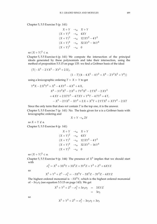
B.3. GRADED RINGS AND MODULES 489
Chapter 5, 5.5 Exercise 5 (p. 141)
X + Y →a X + Y(X + Y)2 →a 4XY
(X + Y)3 →a 12 XY2 − 4 Y3
(X + Y)4 →a 32 XY3 − 16 Y4
(X + Y)5 →a 0
so (X + Y)5 ∈ a.
Chapter 5, 5.5 Exercise 6 (p. 141) We compute the intersection of the principalideals generated by these polynomials and take their intersection, using themethod of proposition 5.5.15 on page 135: we find a Gröbner basis of the ideal
(T(−X3 − 2 YX2 − XY2 + 2 X),
(1− T)(4− 4 X2 − 4 Y2 + X4 − 2 Y2X2 + Y4))
using a lexicographic ordering T X Y to get
Y4X− 2 X3Y2 + X5 − 4 XY2 − 4 X3 + 4 X,
X4 − 3 Y2X2 − 2 X2 + TY2X2 − 2 TX2 − 2 XY3
+ 4 XY + 2 XTY3 − 4 TXY + Y4T − 4 TY2 + 4 T,
− X3 − 2 YX2 − XY2 + 2 X + X3T + 2 YTX2 + XTY2 − 2 XT
Since the only term that does not contain T is the top one, it is the answer.
Chapter 5, 5.5 Exercise 7 (p. 141) No. The basis given for a is a Gröbner basis withlexicographic ordering and
X + Y →a 2Y
so X + Y /∈ a.
Chapter 5, 5.5 Exercise 8 (p. 141)
X + Y →a X + Y(X + Y)2 →a 4XY
(X + Y)3 →a 12 XY2 − 4 Y3
(X + Y)4 →a 32 XY3 − 16 Y4
(X + Y)5 →a 0
so (X + Y)5 ∈ a.
Chapter 5, 5.5 Exercise 9 (p. 144) The presence of X3 implies that we should startwith
σ31 = X3 + 3X2Y + 3X2Z + 3Y2Z + Y3 + Z3 + 6XYZ
soX3 + Y3 + Z3 − σ3
1 = −3X2Y− 3X2Z− 3Y2Z− 6XYZ
The highest ordered monomial is −3X2Y, which is the highest ordered monomialof −3σ1σ2 (see equation 5.5.15 on page 143). We get
X3 + Y3 + Z3 − σ31 + 3σ1σ2 = 3XYZ
= 3σ3
soX3 + Y3 + Z3 = σ3
1 − 3σ1σ2 + 3σ3
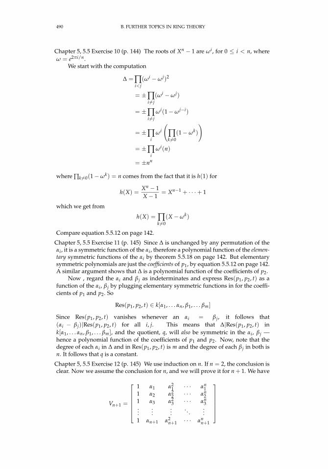
490 B. FURTHER TOPICS IN RING THEORY
Chapter 5, 5.5 Exercise 10 (p. 144) The roots of Xn − 1 are ωi, for 0 ≤ i < n, whereω = e2πi/n.
We start with the computation
∆ =∏i<j
(ωi −ω j)2
= ±∏i 6=j
(ωi −ω j)
= ±∏i 6=j
ωi(1−ω j−i)
= ±∏i
ωi
(∏k 6=0
(1−ωk)
)= ±∏
iωi(n)
= ±nn
where ∏k 6=0(1−ωk) = n comes from the fact that it is h(1) for
h(X) =Xn − 1X− 1
= Xn−1 + · · ·+ 1
which we get from
h(X) = ∏k 6=0
(X−ωk)
Compare equation 5.5.12 on page 142.
Chapter 5, 5.5 Exercise 11 (p. 145) Since ∆ is unchanged by any permutation of theαi, it is a symmetric function of the αi, therefore a polynomial function of the elemen-tary symmetric functions of the αi by theorem 5.5.18 on page 142. But elementarysymmetric polynomials are just the coefficients of p1, by equation 5.5.12 on page 142.A similar argument shows that ∆ is a polynomial function of the coefficients of p2.
Now , regard the αi and β j as indeterminates and express Res(p1, p2, t) as afunction of the αi, β j by plugging elementary symmetric functions in for the coeffi-cients of p1 and p2. So
Res(p1, p2, t) ∈ k[α1, . . . αn, β1, . . . βm]
Since Res(p1, p2, t) vanishes whenever an αi = β j, it follows that(αi − β j)|Res(p1, p2, t) for all i, j. This means that ∆|Res(p1, p2, t) ink[α1, . . . αn, β1, . . . βm], and the quotient, q, will also be symmetric in the αi, β j —hence a polynomial function of the coefficients of p1 and p2. Now, note that thedegree of each αi in ∆ and in Res(p1, p2, t) is m and the degree of each β j in both isn. It follows that q is a constant.
Chapter 5, 5.5 Exercise 12 (p. 145) We use induction on n. If n = 2, the conclusion isclear. Now we assume the conclusion for n, and we will prove it for n + 1. We have
Vn+1 =
1 α1 α2
1 · · · αn1
1 α2 α22 · · · αn
21 α3 α2
3 · · · αn3
......
.... . .
...1 αn+1 α2
n+1 · · · αnn+1
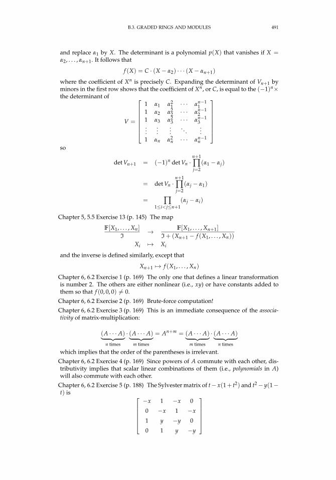
B.3. GRADED RINGS AND MODULES 491
and replace α1 by X. The determinant is a polynomial p(X) that vanishes if X =α2, . . . , αn+1. It follows that
f (X) = C · (X− α2) · · · (X− αn+1)
where the coefficient of Xn is precisely C. Expanding the determinant of Vn+1 byminors in the first row shows that the coefficient of Xn, or C, is equal to the (−1)n×the determinant of
V =
1 α1 α2
1 · · · αn−11
1 α2 α22 · · · αn−1
21 α3 α2
3 · · · αn−13
......
.... . .
...1 αn α2
n · · · αn−1n
so
det Vn+1 = (−1)n det Vn ·n+1
∏j=2
(α1 − αj)
= det Vn ·n+1
∏j=2
(αj − α1)
= ∏1≤i<j≤n+1
(αj − αi)
Chapter 5, 5.5 Exercise 13 (p. 145) The map
F[X1, . . . , Xn]
I→ F[X1, . . . , Xn+1]
I+ (Xn+1 − f (X1, . . . , Xn))
Xi 7→ Xi
and the inverse is defined similarly, except that
Xn+1 7→ f (X1, . . . , Xn)
Chapter 6, 6.2 Exercise 1 (p. 169) The only one that defines a linear transformationis number 2. The others are either nonlinear (i.e., xy) or have constants added tothem so that f (0, 0, 0) 6= 0.
Chapter 6, 6.2 Exercise 2 (p. 169) Brute-force computation!
Chapter 6, 6.2 Exercise 3 (p. 169) This is an immediate consequence of the associa-tivity of matrix-multiplication:
(A · · · A)︸ ︷︷ ︸n times
· (A · · · A)︸ ︷︷ ︸m times
= An+m = (A · · · A)︸ ︷︷ ︸m times
· (A · · · A)︸ ︷︷ ︸n times
which implies that the order of the parentheses is irrelevant.
Chapter 6, 6.2 Exercise 4 (p. 169) Since powers of A commute with each other, dis-tributivity implies that scalar linear combinations of them (i.e., polynomials in A)will also commute with each other.
Chapter 6, 6.2 Exercise 5 (p. 188) The Sylvester matrix of t− x(1+ t2) and t2− y(1−t) is
−x 1 −x 0
0 −x 1 −x
1 y −y 0
0 1 y −y
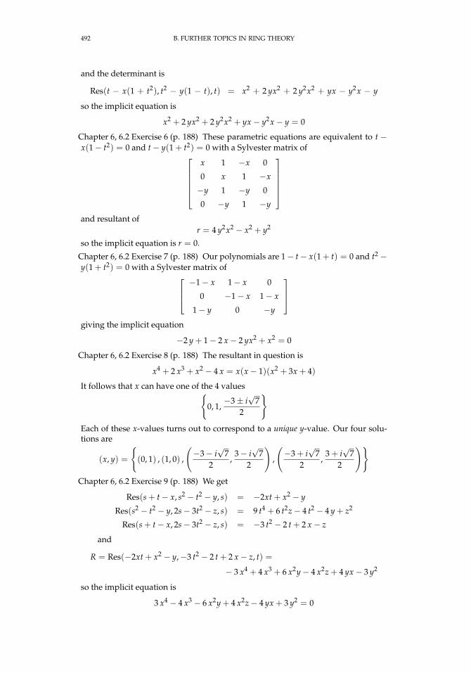
492 B. FURTHER TOPICS IN RING THEORY
and the determinant is
Res(t − x(1 + t2), t2 − y(1 − t), t) = x2 + 2 yx2 + 2 y2x2 + yx − y2x − y
so the implicit equation is
x2 + 2 yx2 + 2 y2x2 + yx− y2x− y = 0
Chapter 6, 6.2 Exercise 6 (p. 188) These parametric equations are equivalent to t −x(1− t2) = 0 and t− y(1 + t2) = 0 with a Sylvester matrix of
x 1 −x 0
0 x 1 −x
−y 1 −y 0
0 −y 1 −y
and resultant of
r = 4 y2x2 − x2 + y2
so the implicit equation is r = 0.
Chapter 6, 6.2 Exercise 7 (p. 188) Our polynomials are 1− t− x(1 + t) = 0 and t2 −y(1 + t2) = 0 with a Sylvester matrix of −1− x 1− x 0
0 −1− x 1− x
1− y 0 −y
giving the implicit equation
−2 y + 1− 2 x− 2 yx2 + x2 = 0
Chapter 6, 6.2 Exercise 8 (p. 188) The resultant in question is
x4 + 2 x3 + x2 − 4 x = x(x− 1)(x2 + 3x + 4)
It follows that x can have one of the 4 values0, 1,−3± i
√7
2
Each of these x-values turns out to correspond to a unique y-value. Our four solu-tions are
(x, y) =
(0, 1) , (1, 0) ,
(−3− i
√7
2,
3− i√
72
),
(−3 + i
√7
2,
3 + i√
72
)Chapter 6, 6.2 Exercise 9 (p. 188) We get
Res(s + t− x, s2 − t2 − y, s) = −2xt + x2 − y
Res(s2 − t2 − y, 2s− 3t2 − z, s) = 9 t4 + 6 t2z− 4 t2 − 4 y + z2
Res(s + t− x, 2s− 3t2 − z, s) = −3 t2 − 2 t + 2 x− z
and
R = Res(−2xt + x2 − y,−3 t2 − 2 t + 2 x− z, t) =
− 3 x4 + 4 x3 + 6 x2y− 4 x2z + 4 yx− 3 y2
so the implicit equation is
3 x4 − 4 x3 − 6 x2y + 4 x2z− 4 yx + 3 y2 = 0
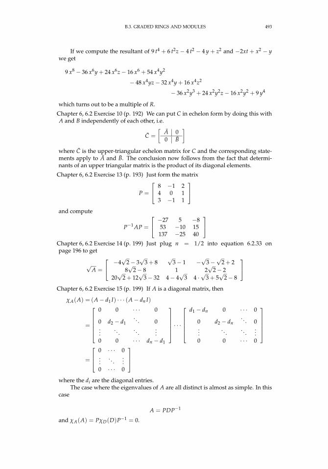
B.3. GRADED RINGS AND MODULES 493
If we compute the resultant of 9 t4 + 6 t2z− 4 t2 − 4 y + z2 and −2xt + x2 − ywe get
9 x8 − 36 x6y + 24 x6z− 16 x6 + 54 x4y2
− 48 x4yz− 32 x4y + 16 x4z2
− 36 x2y3 + 24 x2y2z− 16 x2y2 + 9 y4
which turns out to be a multiple of R.
Chapter 6, 6.2 Exercise 10 (p. 192) We can put C in echelon form by doing this withA and B independently of each other, i.e.
C =
[A 00 B
]where C is the upper-triangular echelon matrix for C and the corresponding state-ments apply to A and B. The conclusion now follows from the fact that determi-nants of an upper triangular matrix is the product of its diagonal elements.
Chapter 6, 6.2 Exercise 13 (p. 193) Just form the matrix
P =
8 −1 24 0 13 −1 1
and compute
P−1 AP =
−27 5 −853 −10 15
137 −25 40
Chapter 6, 6.2 Exercise 14 (p. 199) Just plug n = 1/2 into equation 6.2.33 onpage 196 to get
√A =
−4√
2− 3√
3 + 8√
3− 1 −√
3−√
2 + 28√
2− 8 1 2√
2− 220√
2 + 12√
3− 32 4− 4√
3 4 ·√
3 + 5√
2− 8
Chapter 6, 6.2 Exercise 15 (p. 199) If A is a diagonal matrix, then
χA(A) = (A− d1 I) · · · (A− dn I)
=
0 0 · · · 0
0 d2 − d1. . . 0
.... . .
. . ....
0 0 · · · dn − d1
· · ·
d1 − dn 0 · · · 0
0 d2 − dn. . . 0
.... . .
. . ....
0 0 · · · 0
=
0 · · · 0...
. . ....
0 · · · 0
where the di are the diagonal entries.
The case where the eigenvalues of A are all distinct is almost as simple. In thiscase
A = PDP−1
and χA(A) = PχD(D)P−1 = 0.
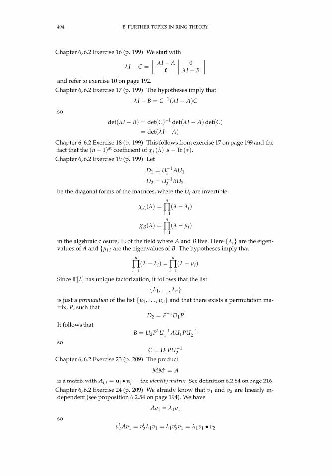
494 B. FURTHER TOPICS IN RING THEORY
Chapter 6, 6.2 Exercise 16 (p. 199) We start with
λI − C =
[λI − A 0
0 λI − B
]and refer to exercise 10 on page 192.
Chapter 6, 6.2 Exercise 17 (p. 199) The hypotheses imply that
λI − B = C−1(λI − A)C
so
det(λI − B) = det(C)−1 det(λI − A)det(C)
= det(λI − A)
Chapter 6, 6.2 Exercise 18 (p. 199) This follows from exercise 17 on page 199 and thefact that the (n− 1)st coefficient of χ∗(λ) is −Tr (∗).
Chapter 6, 6.2 Exercise 19 (p. 199) Let
D1 = U−11 AU1
D2 = U−12 BU2
be the diagonal forms of the matrices, where the Ui are invertible.
χA(λ) =n
∏i=1
(λ− λi)
χB(λ) =n
∏i=1
(λ− µi)
in the algebraic closure, F, of the field where A and B live. Here λi are the eigen-values of A and µi are the eigenvalues of B. The hypotheses imply that
n
∏i=1
(λ− λi) =n
∏i=1
(λ− µi)
Since F[λ] has unique factorization, it follows that the list
λ1, . . . , λnis just a permutation of the list µ1, . . . , µn and that there exists a permutation ma-trix, P, such that
D2 = P−1D1P
It follows thatB = U2P1U−1
1 AU1PU−12
soC = U1PU−1
2Chapter 6, 6.2 Exercise 23 (p. 209) The product
MMt = A
is a matrix with Ai,j = ui •uj — the identity matrix. See definition 6.2.84 on page 216.
Chapter 6, 6.2 Exercise 24 (p. 209) We already know that v1 and v2 are linearly in-dependent (see proposition 6.2.54 on page 194). We have
Av1 = λ1v1
sovt
2 Av1 = vt2λ1v1 = λ1vt
2v1 = λ1v1 • v2
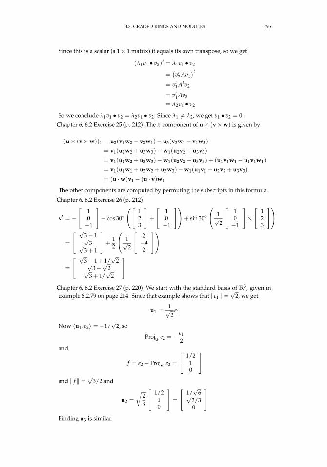
B.3. GRADED RINGS AND MODULES 495
Since this is a scalar (a 1× 1 matrix) it equals its own transpose, so we get
(λ1v1 • v2)t = λ1v1 • v2
=(vt
2 Av1)t
= vt1 Atv2
= vt1 Av2
= λ2v1 • v2
So we conclude λ1v1 • v2 = λ2v1 • v2. Since λ1 6= λ2, we get v1 • v2 = 0 .
Chapter 6, 6.2 Exercise 25 (p. 212) The x-component of u× (v×w) is given by
(u× (v×w))1 = u2(v1w2 − v2w1)− u3(v3w1 − v1w3)
= v1(u2w2 + u3w3)−w1(u2v2 + u3v3)
= v1(u2w2 + u3w3)−w1(u2v2 + u3v3) + (u1v1w1 − u1v1w1)
= v1(u1w1 + u2w2 + u3w3)−w1(u1v1 + u2v2 + u3v3)
= (u ·w)v1 − (u · v)w1
The other components are computed by permuting the subscripts in this formula.
Chapter 6, 6.2 Exercise 26 (p. 212)
v′ = − 1
0−1
+ cos 30
123
+
10−1
+ sin 30
1√2
10−1
× 1
23
=
√
3− 1√3√
3 + 1
+12
1√2
2−42
=
√
3− 1 + 1/√
2√3−√
2√3 + 1/
√2
Chapter 6, 6.2 Exercise 27 (p. 220) We start with the standard basis of R3, given inexample 6.2.79 on page 214. Since that example shows that ‖e1‖ =
√2, we get
u1 =1√2
e1
Now 〈u1, e2〉 = −1/√
2, so
Proju1e2 = − e1
2and
f = e2 − Proju1e2 =
1/210
and ‖ f ‖ =
√3/2 and
u2 =
√23
1/210
=
1/√
6√2/30
Finding u3 is similar.

496 B. FURTHER TOPICS IN RING THEORY
Chapter 6, 6.3 Exercise 1 (p. 228) It A is not principal, then any free basis of A mustcontain at least two elements x, y ∈ R. The equation
y · x− x · y = 0
implies that they can’t be part of a free basis (i.e., all elements of R may be used ascoefficients in linear combinations). If x is a non-zero divisor, then R · x ∼= R.
Chapter 6, 6.3 Exercise 2 (p. 228) Define f to send m (mod A) to f (m) (mod f )(A)for all m ∈ M1. This is well-defined because m ∈ A implies that f (m) ∈ f (A).
Chapter 6, 6.3 Exercise 3 (p. 233) This follows from
F = ker (pk×) : M→ M
so it must be preserved under an isomorphism as well as T = M/F, so it is uniquelydefined. The factor R1 = R/(g1) is the kernel of
g1×: T → T
Define Tj = T/Rj−1 — this must be preserved under any isomorphism of the orig-inal M. The factor Rj+1 is the kernel of
gj+1×: Tj → Tj
so it is also preserved under isomorphisms of M.
Chapter 6, 6.3 Exercise 4 (p. 233) It is 2 0 00 6 00 0 12
with
S =
0 0 10 1 01 0 −5
, T =
3 −2 4−1 3 −2
2 −2 3
Chapter 6, 6.3 Exercise 6 (p. 238) This follows immediately from exercise 18 onpage 199.
Chapter 6, 6.3 Exercise 7 (p. 238) This follows by a straightforward induction. It isclearly true for n = 1. If we assume the result for n− 1 and multiply
λn−1 0 0 · · · 0
(n− 1)λn−1 λn−1 . . .. . .
...
0 (n− 1)λn−1 . . .. . . 0
... · · · . . . λn−1 00 · · · 0 (n− 1)λn−1 λn−1
λ 0 0 · · · 0
1 λ. . .
. . ....
0 1. . .
. . . 0... · · · . . . λ 00 · · · 0 1 λ
we get the expected result.
Chapter 6, 6.3 Exercise 8 (p. 239) We know that
P−1 AP =
1 0 0 0 00 2 0 0 00 1 2 0 00 0 0 3 00 0 0 1 3
= J
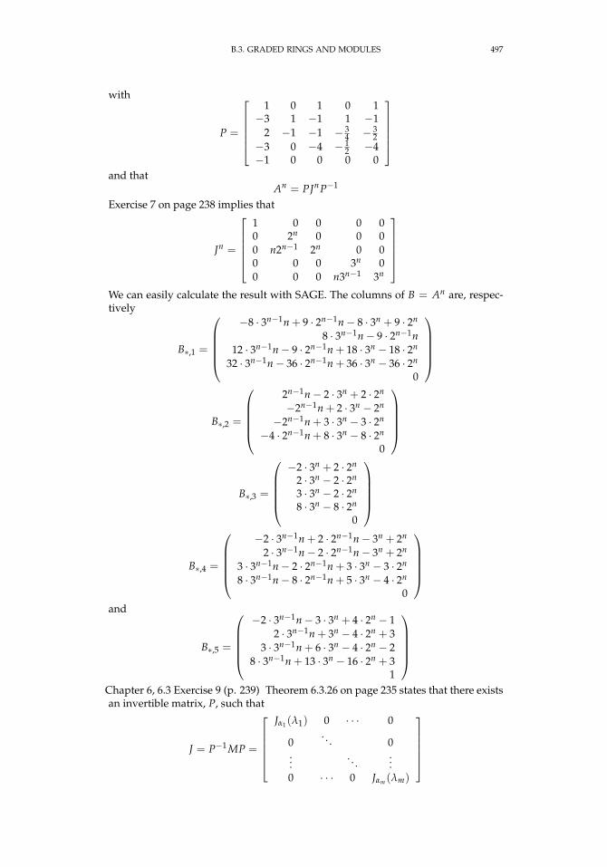
B.3. GRADED RINGS AND MODULES 497
with
P =
1 0 1 0 1−3 1 −1 1 −1
2 −1 −1 − 34 − 3
2−3 0 −4 − 1
2 −4−1 0 0 0 0
and that
An = PJnP−1
Exercise 7 on page 238 implies that
Jn =
1 0 0 0 00 2n 0 0 00 n2n−1 2n 0 00 0 0 3n 00 0 0 n3n−1 3n
We can easily calculate the result with SAGE. The columns of B = An are, respec-tively
B∗,1 =
−8 · 3n−1n + 9 · 2n−1n− 8 · 3n + 9 · 2n
8 · 3n−1n− 9 · 2n−1n12 · 3n−1n− 9 · 2n−1n + 18 · 3n − 18 · 2n
32 · 3n−1n− 36 · 2n−1n + 36 · 3n − 36 · 2n
0
B∗,2 =
2n−1n− 2 · 3n + 2 · 2n
−2n−1n + 2 · 3n − 2n
−2n−1n + 3 · 3n − 3 · 2n
−4 · 2n−1n + 8 · 3n − 8 · 2n
0
B∗,3 =
−2 · 3n + 2 · 2n
2 · 3n − 2 · 2n
3 · 3n − 2 · 2n
8 · 3n − 8 · 2n
0
B∗,4 =
−2 · 3n−1n + 2 · 2n−1n− 3n + 2n
2 · 3n−1n− 2 · 2n−1n− 3n + 2n
3 · 3n−1n− 2 · 2n−1n + 3 · 3n − 3 · 2n
8 · 3n−1n− 8 · 2n−1n + 5 · 3n − 4 · 2n
0
and
B∗,5 =
−2 · 3n−1n− 3 · 3n + 4 · 2n − 1
2 · 3n−1n + 3n − 4 · 2n + 33 · 3n−1n + 6 · 3n − 4 · 2n − 2
8 · 3n−1n + 13 · 3n − 16 · 2n + 31
Chapter 6, 6.3 Exercise 9 (p. 239) Theorem 6.3.26 on page 235 states that there existsan invertible matrix, P, such that
J = P−1 MP =
Jα1 (λ1) 0 · · · 0
0. . . 0
.... . .
...0 · · · 0 Jαm (λm)
498 B. FURTHER TOPICS IN RING THEORY
is the Jordan Canonical Form. Furthermore
Jn = P−1 MnP = I =
Jα1 (λ1)
n 0 · · · 0
0. . . 0
.... . .
...0 · · · 0 Jαm (λm)n
Exercise 7 on page 238 shows that a Jordan block Jα(λ)n = I if and only if α = 1.The statement about the eigenvalues is clear.
Chapter 6, 6.3 Exercise 10 (p. 245) This is basic linear algebra: U is the nullspace ofthe linear map V →W and the image is all of W.
Chapter 6, 6.3 Exercise 11 (p. 245) Suppose V is a vector-space over an infinite field,k, and
V =n⋃
i=1Vi
where the Vi are proper subspaces. Without loss of generality, assume this decom-position is minimal (none of the Vi’s are contained in a union of the others).
If x ∈ V1 and y ∈ V \ V1, then x + r · y ∈ V as r ∈ k runs over an (infinite)number of nonzero values. The Pigeonhole Principle implies that there is a j suchthat
x + r · y ∈ Vj
for an infinite number of values of r. This means that there exist r1 6= r2 ∈ k withx + r1 · y, x + r2 · y ∈ Vj which implies that (x + r1 · y)− (x + r2 · y) = (r1− r2) · y ∈Vj so y ∈ Vj. We conclude that x ∈ Vj as well. Since x was an arbitrary element ofV1, this means that
V1 ⊂n⋃
i=2Vi
which contradicts the assumption that the original decomposition was minimal.Chapter 6, 6.3 Exercise 12 (p. 245) A finite-dimensional vector-space over afinite field has a finite number of elements, hence is the (finite) union of theone-dimensional subspaces generated by these elements,
Chapter 6, 6.3 Exercise 13 (p. 245) Just apply proposition 6.3.16 on page 226 to thediagram
Pgzz
Mf// P
Chapter 6, 6.3 Exercise 14 (p. 245) If x ∈ R annihilates M2, it annihilates any sub-module and quotient so
Ann(M2) ⊂ Ann(M1) ∩Ann(M3)
If x ∈ Ann(M1), y ∈ Ann(M3), and m ∈ M2, then y ·m ∈ M1, since its image in M3is zero. Then x · (y ·m)) = 0, so
Ann(M1) ·Ann(M3) ⊂ Ann(M2)
Chapter 6, 6.3 Exercise 15 (p. 245) We claim that the map
(q, h): U ⊕W → V
is an isomorphism. Suppose (u, v) maps to 0 in V, so q(u) = −h(v). If we mapthis via p, we get p q(u) = −p h(v). Since p q = 0, we get p h(v) = 0 which
B.3. GRADED RINGS AND MODULES 499
implies that v = 0 (since p h = 1). Since q is injective, this also implies that u = 0.So the map, (q, h), is injective.
Suppose v ∈ V is any element and let z = v− h p(v). Then p(z) = p(v)− p h p(v) = p(v)− p(v) = 0. This implies that z = q(u) for some u ∈ U and
v = (q, h)(z, h(v))
so the map is also surjective.
Chapter 6, 6.3 Exercise 16 (p. 246) This follows immediately from exercises 13 onpage 245 and 15 on page 245.
Chapter 6, 6.4 Exercise 2 (p. 248) This follows immediately from the AscendingChain Condition (in proposition 5.4.2 on page 122) and corollary 6.4.8 on page 248.
Chapter 6, 6.4 Exercise 3 (p. 249) The non-zero-divisors of R × S is the set (r, s)where r is a non-zero-divisor of R and s is a non-zero-divisor of S.
Chapter 6, 6.4 Exercise 4 (p. 249) Let ann(m) ⊂ R be the annihilator of m — anideal. Then m goes to 0 in Ma if and only if ann(m) 6⊂ a (see definition 6.4.9 onpage 248). But proposition 5.2.11 on page 115 shows that every ideal is contained insome maximal ideal.
Chapter 6, 6.4 Exercise 5 (p. 249) This follows immediately from exercise 4 onpage 249.
Chapter 6, 6.4 Exercise 6 (p. 249) The general element of F is of the form
f =a0 + a1X + · · ·b0 + b1X + · · ·
Suppose ai is the lowest indexed coefficient in the numerator that is nonzero and bjis the corresponding one in the denominator. Then
f =Xi(ai + ai+1X + · · · )X j(bj + bj+1X + · · · ) = Xi−j ai + ai+1X + · · ·
bj + bj+1X + · · ·where bj 6= 0 so that the denominator is a unit in R (see proposition 5.1.9 on
page 109). Set α = i− j and r = (ai + ai+1X + · · · )(
bj + bj+1X + · · ·)−1
.
Chapter 6, 6.5 Exercise 1 (p. 257) Suppose s−1x ∈ S−1T is integral over S−1R. Thenit satisfies an equation
(s−1x)n + an−1(s−1x)n−1 + · · ·+ a0 = 0
where the ai ∈ S−1R. Let s ∈ S be able to clear the denominators of all of the ai.Multiplying this equation by (ss)n gives
(sx)n + an−1ss(sx)n−1 + · · ·+ sn sa0 = 0
so sx ∈ R is integral over R, and (ss)−1(sx) = s−1x is integral over S−1R.
Chapter 6, 6.5 Exercise 2 (p. 257) Let
xn + an−1xn−1 + · · ·+ a0 = 0
be the minimal polynomial (see definition 7.1.8 on page 261) of x with ai ∈ F. Ifs ∈ R can clear the denominators of the ai, multiply this equation by sn to get
snxn + snan−1xn−1 + · · ·+ sna0 = (sx)n + an−1s(sx)n−1 + · · ·+ sna0
= 0
so sx is integral over R.

500 B. FURTHER TOPICS IN RING THEORY
Chapter 6, 6.5 Exercise 3 (p. 257) Clearly, any element x ∈ F that is integral over Ris also integral over T. On the other hand, if x is integral over T, it is also integralover R because of statement 2 of proposition 6.5.5 on page 251 (the degree of themonic polynomial over R will usually be higher than that over T). It follows thatthe integral closures will be the same.
Chapter 7, 7.1 Exercise 1 (p. 263) Let p(X) ∈ F[X] be the minimum polynomial ofα. Its being of degree n implies that F[X]/(p(X)) = F[α] = F(α) is a degree-nextension of F. The conclusion follows from proposition 7.1.6 on page 261.
Chapter 7, 7.1 Exercise 2 (p. 263) Whenever one gets X3, it must be replaced by−3− 3X, giving the result
ad− 3ce− 3b f + X(ae + bd− 3ce− 3c f − 3b f ) + X2(a f + be + cd− 3c f )
Chapter 7, 7.2 Exercise 1 (p. 269) We claim that F(X) = F(X2) · 1⊕ F(X2) · X as avector space. If
u =p(X)
q(X)
we can writeq(X) = a(X2) + X · b(X2)
— just separate the terms with odd powers of X from the others. Now, we get
u =p(X)
q(X)· a(X2)− X · b(X2)
a(X2)− X · b(X2)=
p(X)(a(X2)− X · b(X2))
a(X2)2 − X2 · b(X2)2
Now, write the numerator as
p(X) = c(X2) + X · d(X2)
so we get
u =R(Y)S(Y)
+ X · T(Y)S(Y)
where
S(Y) = a(Y)2 −Y · b(Y)2
R(Y) = c(Y)a(Y)−Y · b(Y)d(Y)T(Y) = a(Y)d(Y)− c(Y)b(Y)
Chapter 7, 7.2 Exercise 2 (p. 269) The number 21/3 satisfies the equation
X3 − 2 = 0
and Eisenstein’s Criterion (theorem 5.6.8 on page 149) shows that this is irreducible.It follows that X3 − 2 is the minimal polynomial of 21/3.
Set Q(21/3) = Q[X]/(X3− 2). We would like to find the multiplicative inverseof the polynomial
X2 − X + 1modulo X3 − 2. We can use the extended Euclidean algorithm (algorithm 3.1.12 onpage 17) for this. Dividing X3 − 2 by X2 − X + 1 gives a quotient of q1(X) = X + 1and a remainder of −3. We’re done since
(X + 1) · (X2 − X + 1)− 1 · (X3 − 2) = 3
or13(X + 1) · (X2 − X + 1)− 1
3· (X3 − 2) = 1
so, modulo X3 − 2, we get 13 (X + 1) · (X2 − X + 1) = 1 which implies that
13(21/3 + 1) =
122/3 − 21/3 + 1
∈ Q(21/3) = Q[21/3]
B.3. GRADED RINGS AND MODULES 501
Chapter 7, 7.2 Exercise 3 (p. 269) Just follow the proof of theorem 7.2.13 onpage 268. The minimal polynomials of
√2 and
√3 are, respectively, X2 − 2 and
X2 − 3. Their roots (i.e., the αi and β j in the proof) are
±√
2,±√
3
and the set of elements of Q we must avoid are√
2√3∈ Q[
√2,√
3] \Q
Since this is not a rational number, it follows that we can pick any nonzero rationalnumber for our c. We pick c = 1 and γ =
√2 +√
3.So
Q[√
2,√
3] = Q[√
2 +√
3]
To find the minimal polynomial, we refer to example 7.3.1 on page 270.
Chapter 7, 7.2 Exercise 4 (p. 269) One obvious root of X3 − 2 ∈ Q[X], is X = 21/3,so we try the field extension
Q[21/3]
Since 21/3 is a root of X3 − 2, we get (X− 21/3)|(X3 − 2) with a quotient of
X2 + 21/3 · X + 22/3
and if we set X = Y · 21/3, this becomes
22/3 · (Y2 + Y + 1)
The roots ofY2 + Y + 1 = 0
are
ω, ω2 =−1±
√−3
2which are the cube-roots of 1 (other than 1 itself). So our splitting field is
Q[21/3, ω]
of degree 6 over Q.
Chapter 7, 7.3 Exercise 1 (p. 271) We find a Gröbner basis for a = (X2 − 2, Y3 −2, A− X−Y) with lexicographic order with
X Y A
to get
a = (−4− 24 A + 12 A2 − 6 A4 − 4 A3 + A6,
− 364 + 152 A− 156 A2 + 9 A4
− 160 A3 + 24 A5 + 310 Y,
364− 462 A + 156 A2 − 9 A4
+ 160 A3 − 24 A5 + 310 X)
so the minimal polynomial of α is
α6 − 6α4 − 4α3 + 12α2 − 24α− 4 = 0
502 B. FURTHER TOPICS IN RING THEORY
Chapter 7, 7.3 Exercise 2 (p. 274) The minimal polynomial is X3 − 2 and we get abasis of 1, 21/3, 22/3. If γ = a + b21/3 + c22/3, then the effect of γ on the basis isgiven by
γ · 1 = a + b21/3 + c22/3
γ · 21/3 = 2c + a21/3 + b22/3
γ · 22/3 = 2b + 2c21/3 + a22/3
which gives a matrix
mγ =
a 2c 2bb a 2cc b a
with a determinant
NH/F(γ) = a3 − 6 acb + 2 b3 + 4 c3
and characteristic polynomial
χγ(X) = X3 − 3 aX2 −(
6 cb− 3 a2)
X− a3 + 6 acb− 2 b3 − 4 c3
Chapter 7, 7.3 Exercise 3 (p. 274) In this case, our basis for H over Q is1,√
2,√
3,√
6. If γ = a + b√
2 + c√
3 + d√
6 is a general element, its effect on abasis is
γ · 1 = a + b√
2 + c√
3 + d√
6
γ ·√
2 = 2b + a√
2 + 2d√
3 + c√
6
γ ·√
3 = 3c + 3d√
2 + a√
3 + b√
6
γ ·√
6 = 6d + 3c√
2 + 2b√
3 + a√
6
which gives a matrix
mγ =
a 2b 3c 6db a 3d 3cc 2d a 2bd c b a
with a determinant
NH/F(γ) = a4 − 4 a2b2 + 48 adbc− 12 d2a2 − 6 a2c2
+ 4 b4 − 24 d2b2 − 12 b2c2 + 9 c4 − 36 c2d2 + 36 d4
and characteristic polynomial
χH/F(γ) = X4 − 4 aX3 +(−12 d2 − 6 c2 − 4 b2 + 6 a2
)X2
+(−48 dbc + 24 d2a + 12 ac2 + 8 ab2 − 4 a3
)X
a4 − 4 a2b2 + 48 adbc− 12 d2a2 − 6 a2c2
+ 4 b4 − 24 d2b2 − 12 b2c2 + 9 c4 − 36 c2d2 + 36 d4
Chapter 7, 7.4 Exercise 1 (p. 277) If α∣∣ β in Z[γ], then β = α · t where t ∈ Z[γ] and
t =n−1
∑i=0
ciγi
with ci ∈ Z. Since α ∈ Z, we have
α · t =n−1
∑i=0
αciγi
B.3. GRADED RINGS AND MODULES 503
and this is in Z ⊂ Z[γ] if and only if ci = 0 for i > 0. This means that α∣∣ β in Z.
Chapter 7, 7.4 Exercise 2 (p. 277) deg Φn(X) = φ(n) — see definition 3.3.1 onpage 21.
Chapter 7, 7.5 Exercise 1 (p. 285) Suppose
f (X) = Xn + an−1Xn−1 + · · ·+ a0
(after dividing by an if necessary) and embed F in its algebraic closure, F. We get
f (X) =n
∏j=1
(X− αj)
and the splitting field of f (X) is just
F[α1, . . . , αn] ⊂ F
which is unique in F. The conclusion follows from theorem 7.5.3 on page 281.
Chapter 7, 7.5 Exercise 2 (p. 285) The characteristic polynomial of γ was computedin the solution to 2 on page 274 (setting c = 0)
χγ(X) = X3 − 3 aX2 + 3 a2X− a3 − 2 b3
and this is also the minimal polynomial of γ. One factor of this must be X − γ, sowe take the quotient
X3 − 3 aX2 + 3 a2X− a3 − 2 b3
X− γ
= X2 + X(γ− 3a) + γ(γ− 3a) + 3a2
= X2 + (−2a + b 21/3)X + a2 − ab 21/3 + b2 22/3
regarding it as a polynomial with coefficients in C. The roots of this quadratic equa-tion are
X = a + b
(−1±
√−3
2
)21/3 = a + b21/3ω j
where ω = e2πi/3 is a primitive cube root of 1 and j = 1, 2. Since ω /∈ Q[21/3], theseconjugates do not lie in Q[21/3]. This is why we need to go to an algebraic closure ofthe field.
Chapter 7, 7.5 Exercise 3 (p. 285) Yes! The algebraic numbers, Q, are an algebraicextension of Q but of infinite degree.
Chapter 7, 7.5 Exercise 4 (p. 285) Oddly, yes. If
Q = Q(α1, . . . )
then
Q =∞⋃
i=1Q(α1, . . . , αi) =
∞⋃i=1
Q[α1, . . . , αi] = Q[α1, . . . ]
Chapter 7, 7.6 Exercise 2 (p. 288) R(x) = x7 + x6, S(x) = x2 + x + 1
Chapter 7, 7.7 Exercise 1 (p. 293) Suppose π is algebraic. Then so is πi and eπi
should be transcendental, by the Lindemann–Weierstrass theorem. But eπi = −1(see Euler’s Formula, theorem 2.1.2 on page 7), which is algebraic. This is acontradiction.

504 B. FURTHER TOPICS IN RING THEORY
Chapter 7, 7.7 Exercise 2 (p. 293) The algebraic closure of Q is the algebraic num-bers, Q, which is countable. If F is a countable field F(X) is also a countable fieldand a simple induction shows that
F(X1, . . . , Xn)
is also countable for any n. If S = X1, . . . is a countable set of indeterminates,then
F(S) =∞⋃
i=1F(X1, . . . , Xi)
is also countable. It follows that an uncountable field like C must have an uncount-able degree of transcendence over Q.
Chapter 8, 8.3 Exercise 1 (p. 301) This follows immediately from the definition ofF(α1, . . . , αk): if x ∈ F(α1, . . . , αk) then
x =∑k
i=1 ∑nij=0 ci,jα
ji
∑ki=1 ∑mi
j=0 di,jαji
where ci,j, di,j ∈ F. All of the elements here are fixed by f .
Chapter 8, 8.6 Exercise 1 (p. 311) Suppose
(B.3.9) F ⊂ F1 ⊂ · · · ⊂ Fk = E
is a tower of radical extensions for E. We will refine it to one with the requiredproperties — i.e. we will insert new terms between the old ones.
If Fi+1 = Fi(α), where αn = 1 and n = p ·m, where p is a prime, set E1 = Fi(β)where β = αm, and consider the series
Fi ⊂ E1 ⊂ Fi+1
Since βp = 1, Fi ⊂ E1 is pure of type p.Now Fi+1 = E1(α), where αm ∈ F1. If m is not a prime, continue this construc-
tion, inserting new subfields and stripping off a prime in each step.We will eventually arrive at a sequence of subfields
Fi ⊂ E1 ⊂ · · · ⊂ Ek ⊂ Fi+1
where each extension is pure of prime type.Apply this construction to all terms of equation B.3.9 to get the required result.
Chapter 8, 8.6 Exercise 2 (p. 311) Since F ⊂ E is finite, it is algebraic (see proposi-tion 7.2.2 on page 264), so
E = F(α1, . . . , αk)
If fi(X) ∈ F[X] is the minimal polynomial of αi set
f (X) =k
∏i=1
fi(X)
and define G to be the splitting field of f (X) (see corollary 7.2.4 on page 264).
Chapter 8, 8.6 Exercise 4 (p. 311) Since G is the splitting field of
f (X) =k
∏i=1
fi(X)
it contains the conjugates of each of the αi — and these are the images of the αi underthe Galois group of G over F.
If Gal(G/F) = g1 . . . , gn we define Ei = gi(E).
B.3. GRADED RINGS AND MODULES 505
Chapter 8, 8.6 Exercise 5 (p. 312) Since
E
F
is a radical extension, we use exercise 1 on page 311 to conclude that it can beresolved into a sequence of pure extensions via primes, pi. Each has the formEi+1 = Ei(αi), where α
pii ∈ Ei. The conjugates of αi are precisely αi · ω j
i , whereωi
i = 1 — i.e. we must adjoin appropriate roots of unity to get a splitting field.These adjunctions are also pure of prime order, so the extension
G
F
must also be radical.
Chapter 8, 8.8 Exercise 1 (p. 319) We prove this by induction on |G|. If |G| > 1, thenZ(G) > 1 by Burnside’s Theorem 4.7.14 on page 79. If Z(G) = G, then G is abelian,so it is solvable. Otherwise, G/Z(G) is a smaller p-group, which is solvable bythe inductive hypothesis. Since Z(G) is also solvable (because it’s abelian), we useexercise 6 on page 87 to conclude that G is solvable.
Chapter 9, 9.1 Exercise 1 (p. 322) If y = (a, b) ∈ A ⊕ A, then y∗ = (a∗,−b) andequation 9.1.1 on page 322 gives
yy∗ = aa∗ + bb∗
y∗y = a∗a + b∗b
so the right inverse is
y−1 =y∗
yy∗
and the left inverse isy∗
y∗y= y−1
Chapter 9, 9.1 Exercise 2 (p. 322) If u = (a, b) and v = (c, d), then
uv = (ac− d∗b, da + bc∗)
and
(B.3.10) (uv)∗ = (c∗a∗ − b∗d,−da− bc∗)
using equation 9.1.2 on page 322. Now u∗ = (a∗,−b) and v∗ = (c∗,−d), and directcomputation, using equation 9.1.2 on page 322 shows that v∗u∗is equal to the rightside of equation B.3.10.
Chapter 9, 9.1 Exercise 3 (p. 322) Suppose a, b are nonzero and
ab = 0
If we have a−1 · a = 1 and multiply the equation above by a−1, we get
a−1(ab) = 0 6= (a−1a)b = b
In other words, if the algebra fails to be associative, this can easily happen.
Chapter 9, 9.1 Exercise 4 (p. 322) If a = x · b and u · b = 0 with u 6= 0, then a =(x + u) · b so that quotients are not unique.
506 B. FURTHER TOPICS IN RING THEORY
Chapter 9, 9.1 Exercise 5 (p. 322) If a ∈ A is nonzero, then a×: A → A defines alinear transformation. Since A has no zero-divisors, the kernel of this linear trans-formation is zero. Corollary 6.2.33 on page 180 implies that a× is 1-1, so it mapssome element, a−1, to 1.
Chapter 9, 9.1 Exercise 6 (p. 323) If c ∈ A, then mx(c) = x · c, in general. The defini-tion of matrix-product implies that
mxmy = x · (y · c))— see section 6.2.2 on page 167. If A is associative, x · (y · c)) = (x · y) · c, so thatmx·y = mxmy. Otherwise, we have mx·y 6= mxmy in general, and there is no obviousrelationship.
Chapter 9, 9.2 Exercise 1 (p. 330) No! If it was valid, it would imply that multipli-cation of exponentials is commutative, whereas equation 9.2.6 on page 327 impliesthat
eα·u1 · eβ·u2 − eβ·u2 · eα·u1 = 2 sin α sin β · u1 × u2 6= 0
in general.Chapter 9, 9.2 Exercise 2 (p. 330) In several places, including the claim that xy =yx =⇒ x−1y = yx−1, and equation 9.2.7 on page 329.
Chapter 9, 9.2 Exercise 3 (p. 330) It suffices to check it on quaternion units with thecorrespondence:
1↔ (1, 0)
i↔ (i, 0)
j↔ (0, 1)
k↔ (0, i)
Chapter 9, 9.2 Exercise 4 (p. 330) The matrix is of the form[0 0 0 00 C1 C2 C3
]so the rotation is given by (see equation 6.2.7 on page 168)
M =[
C1 C2 C3]
where
C1 = x · i · x−1 = 0 + i(a2 + b2 − c2 − d2) + j(2ad + 2bc) + k(2bd− 2ac)
= 0 + i(1− 2c2 − 2d2) + j(2ad + 2bc) + k(2bd− 2ac)
C2 = x · j · x−1
C3 = x · k · x−1
or
M =
1− 2(c2 + d2) 2(bc− ad) 2(bd + ac)2(ad + bc) 1− 2(b2 + d2) 2(cd− ab)2(bd− ac) 2(cd + ab) 1− 2(b2 + c2)
Chapter 10, 10.1 Exercise 1 (p. 340) This is literally a direct restatement ofthe definition of a product: every pair of morphisms f ∈ homC (W, A) andg ∈ homC (W, B) induces a unique morphism f × g ∈ homC (W, A × B) thatmakes the diagram 10.1.2 on page 336 commute.
Chapter 10, 10.1 Exercise 3 (p. 340) Suppose g1, g2 ∈ homC (C, A) map to the sameelement of homC (C, B), then f g1 = f g2: C → B, which implies (by the defini-tion of monomorphism) that g1 = g2.
B.3. GRADED RINGS AND MODULES 507
Chapter 10, 10.1 Exercise 4 (p. 340) If
f : A→ B
has a kernel, the inclusion of distinct elements of A that differ by an element ofthe kernel are distinct morphisms whose composite with f are the same. The otherconclusion follows by a similar argument.
Chapter 10, 10.2 Exercise 1 (p. 345) It is At, the transpose of A.
Chapter 10, 10.2 Exercise 2 (p. 345) It is an equivalence because of the natural iso-morphism in example 10.2.5 on page 344. It is not an isomorphism of categoriesbecause the finite-dimensional vector-space V∗∗ is not identical to V. If V is infinite-dimensional, it is not even isomorphic.
Chapter 10, 10.3 Exercise 1 (p. 347) Every pair of morphisms
y → xz → x
— i.e., every morphism (y, z)→ ∆x — corresponds to a unique morphism
y ä z→ x
so we get an equivalence
homC×C ((y, z), ∆x) = homC (y ä z, x)
Chapter 10, 10.4 Exercise 1 (p. 356) It is given in theorem 4.10.5 on page 88.
Chapter 10, 10.4 Exercise 2 (p. 356) Definition 10.4.10 on page 352 implies that thereis a natural equivalence
homC∞ (∆∞x, y) = homC (x, lim←− y)
for all x ∈ C and y ∈ C∞.
Chapter 10, 10.4 Exercise 3 (p. 356) This follows immediately from the definition ofthe equivalence relation ∼ in definition 10.4.1 on page 347.
Chapter 10, 10.5 Exercise 2 (p. 360) If a ∈ A is torsion-free then a 7→ x for any x 6= 0defines a nonzero homomorphism. If a is of order n then a 7→ 1/n defines a nonzeromap.
Chapter 10, 10.5 Exercise 3 (p. 361) The sub-object im A ⊂ B maps to A in astraightforward way. The injective property of A implies that this extends to all ofB.
Chapter 10, 10.5 Exercise 4 (p. 361) We already know that
0→ homA (D, A)homA (1,r)−−−−−−→ homA (D, B)
is exact, by exercise 3 on page 340, so we must still show that
homA (D, A)homA (1,r)−−−−−−→ homA (D, B)
homA (1,s)−−−−−−→ homA (D, C)
is exact. If f ∈ homA (D, B) maps to 0 in homA (D, C), then s f = 0. Sincer = ker s, we have a unique morphism D → A that makes
Df//
v $$
B
ArOO
commute. This is precisely the element of homA (D, A) that maps to f .
508 B. FURTHER TOPICS IN RING THEORY
Chapter 10, 10.6 Exercise 1 (p. 372) The hypotheses imply that the composites
R → Mp1−→ M/S→ R
S → Mp2−→ M/R→ S
are the identity maps, so we get a well-defined homomorphism
M(p1,p2)−−−−→ R⊕ S
and this is easily verified to be an isomorphism.Chapter 10, 10.6 Exercise 2 (p. 372) If Q = M/N, we get a short exact sequence
0→ N → M→ Q→ 0
and the conclusion follows from the fact that the sequence
0→ A⊗R N → A⊗R M→ A⊗R Q→ 0
is also exact (because A is flat).Chapter 10, 10.6 Exercise 3 (p. 372) In the top formula, multilinear maps
M× N × T → A
where A is an arbitrary R-module factor through M⊗R (N⊗R T) and (M⊗R N)⊗RT so the universal property of ⊗ implies that they are isomorphic.
To see the second equality, regard M⊗R N and N⊗R M as quotients of Z[M×N] by the ideal generated by the identities in definition 10.6.3 on page 362 andnoting that this ideal is symmetric with respect to factors.
Chapter 10, 10.6 Exercise 4 (p. 373) Corollary 10.6.8 on page 365 implies that
kn ⊗k km = kn·m
so the dimensions are as claimed.If ei is a basis for V and f j is a basis for W then it is not hard to see that
ei ⊗ f j, i = 1, . . . , n, j = 1, . . . , m spans V ⊗k W — just use the identities in defini-tion 10.6.3 on page 362 to express any v⊗w in terms of them. The fact that V ⊗k Wis n ·m-dimensional shows that these elements must be linearly independent too.
To prove the final statement, we must show that the set ei ⊗ f j is linearlyindependent even if there are an infinite number of basis elements. Suppose wehave some linear combination
(B.3.11)n
∑t=1
at(eit ⊗ fkt ) = 0
for at ∈ k. Since only a finite number of terms are involved, this equation reallyinvolves finite-dimensional subspaces of V and W, namely the span of the eit inV and the span of the f jt in W. We have already seen that the eit ⊗ fkt arelinearly independent in this case, so all of the at = 0 in equation B.3.11.
Chapter 10, 10.6 Exercise 5 (p. 373) This is an ns × mt matrix called the Kroneckerproduct of A and B. If
A =
a1,1 · · · a1,n...
. . ....
am,1 · · · am,n
Then
A⊗ B =
a1,1B · · · a1,nB...
. . ....
am,1B · · · am,nB
B.3. GRADED RINGS AND MODULES 509
Chapter 10, 10.6 Exercise 6 (p. 373) We construct a homomorphism
M∗ ⊗ N → homk(M, N)
Let M have basis ei with i = 1, . . . , m, and let N have basis f jwith k = 1, . . . , n.Then M∗ has the dual basis ei defined by
ei(ej) =
0 if i 6= j1 if i = j
and M∗ ⊗ N has a basis ei ⊗ f j. Given an element, m ∈ M, we can evaluate eachbasis element
ei(m) · f j
to define an element of homk(M, N). Since this is bilinear and dim M∗⊗N = nm =dim homk(M, N), it follows that it defines an isomorphism.
Chapter 10, 10.6 Exercise 7 (p. 373) This follows immediately fromproposition 10.6.11 on page 366:
Ra⊗R
Rb=
(Ra
)/b ·(
Ra
)=
Ra+ b
Chapter 10, 10.6 Exercise 8 (p. 373) We always have a surjective natural map
a⊗R M → a ·Ma⊗m 7→ a ·m
If M is flat, this map is also injective since it is
a → R
⊗M.
Chapter 10, 10.6 Exercise 9 (p. 373) For each i, take the natural maps
zi: Mi → lim−→ Mj
Zi: Mi ⊗R N → lim−→(
Mj ⊗R N)
and form the tensor product of Mi with N to get
zi ⊗ 1: Mi ⊗R N →(
lim−→ Mj
)⊗R N
The universal property of direct limits implies the existence of a unique map
v: lim−→(
Mj ⊗R N)→(
lim−→ Mj
)⊗R N
that makes the diagram
lim−→(
Mj ⊗R N)
v //(
lim−→ Mj
)⊗R N
Mi ⊗R N
ZiOO
Mi ⊗R N
zi⊗1OO
commute. If m⊗ n 6= 0 ∈(
lim−→ Mj
)⊗R N, then m is the image of some mi ∈ Mi
and m⊗ n = v Zi(mi ⊗ n). It follows that v is surjective.
If w ∈ lim−→(
Mj ⊗R N)
is in the kernel of v, then w = Zi(mi ⊗ n) for some i.the commutativity of the diagram implies that (zi ⊗ 1)(mi ⊗ n) = zi(mi)⊗ n = 0,which implies that Zi(mi ⊗ n) = 0 — so v is injective.
510 B. FURTHER TOPICS IN RING THEORY
Chapter 10, 10.6 Exercise 10 (p. 373) The hypotheses imply that
0 // lim−→ Ailim−→ fi// lim−→ Bi
lim−→ gi// lim−→ Ci // 0
0 // Ai
aiOO
fi
// Bi
biOO
gi// Ci
ciOO
// 0
commutes for all i, where we don’t know whether the top row is exact. If x ∈ lim−→ Ci,then x is the image of some xi ∈ Ci. The commutativity of this diagram implies thatx is in the image of bi(g−1
i (xi)). It follows that lim−→ gi is surjective. If x ∈ lim−→ Bi suchthat x ∈ ker lim−→ gi, then x = bi(xi) for some i and ci gi(xi) = 0. The definitionof direct limit implies that there exists N > i such that cN · · · ci(x) = 0, sobN · · · bi(xi) ∈ ker gN . The exactness of the original sequences implies thatbN · · · bi(xi) = fN(yN) and the commutativity of the diagram above impliesthat aN(yN) = x. A similar argument implies that the left end of the upper row isalso exact.
Chapter 10, 10.6 Exercise 11 (p. 373) Consider the map g: (α) → R. This is an inclu-sion and, since S is flat over R
(α)⊗R Sg⊗1−−→ R⊗R S = S
is also an inclusion. Since α is a non-zero-divisor in R, (α) ∼= R and the isomorphismR→ R induced by the inclusion is multiplication by α. This implies that
S = R⊗R S(×α)⊗1=× f (α)−−−−−−−−−→ R⊗R S = S
is also injective, which implies that f (α) ∈ S is a non-zero-divisor.
Chapter 10, 10.6 Exercise 12 (p. 373) Let
(B.3.12) 0→ U1 → U2 → U3 → 0
be a short exact sequence of modules over S. Since we can compose the action ofS on these modules with the homomorphism, f , it is also a short exact sequence ofmodules over R. If we take the tensor product with M⊗R S, we get
0 // U1 ⊗S (M⊗R S) // U2 ⊗S (M⊗R S) //// U3 ⊗S (M⊗R S) //// 0
U1 ⊗R M U2 ⊗R M U3 ⊗R M
which is exact since equation B.3.12 is an exact sequence of R-modules.
Chapter 10, 10.6 Exercise 13 (p. 374)
Chapter 10, 10.6 Exercise 14 (p. 374) For any commutative ring U and any moduleA over U, U ⊗U A = A. This (and the associativity of tensor products) implies that
(S−1R⊗R M)⊗S−1R (S−1R⊗R N) = (S−1R⊗R M)⊗S−1R S−1R⊗R N
= (S−1R⊗R M)⊗R N
= S−1R⊗R M⊗R N
= S−1R⊗R (M⊗R N)
Chapter 10, 10.6 Exercise 15 (p. 374) Since M is projective, it is a direct summand ofa free module, F, so F = M⊕ N for some other projective module, N. Then
F∗ = M∗ ⊕ N∗
Chapter 10, 10.7 Exercise 1 (p. 382) First of all, note that the map V → W is split,i.e. there exists a left-inverse t: W → V so that g t = 1. Any two such splitting
B.3. GRADED RINGS AND MODULES 511
maps differ by a map from V to U. Now define 1− t g: W → ker g = im U orf−1 (1− t g): W → U. We get an isomorphism
( f−1 (1− t g), g): W ∼= U ⊕V
Given a commutative diagram like the one in the statement of the problem, we canlift a map t2: W2 → V2 to get a map t1: W1 → V2 so we get a natural isomorphismfrom Wi to Ui ⊕Vi . The conclusion follows from proposition 10.7.8 on page 377.
Chapter 10, 10.7 Exercise 2 (p. 382)Chapter 10, 10.7 Exercise 3 (p. 382) Just compute
(e2 + 2e4) ∧ e3 ∧ 2e1 ∧ (e2 − e4) = −e2 ∧ e3 ∧ 2e1 ∧ e4
−2e4 ∧ e3 ∧ 2e1 ∧ e2
= −2e1 ∧ e2 ∧ e3 ∧ e4
+4e1 ∧ e2 ∧ e3 ∧ e4
= 2e1 ∧ e2 ∧ e3 ∧ e4
so the determinant is 2.Chapter 11, 11.1 Exercise 2 (p. 388) If x 6= 0 ∈ M, then R · x ⊂ M is a submodule.Chapter 11, 11.1 Exercise 4 (p. 388) Any sub-representation would be one dimen-sional, there is no invariant one-dimensional subspace.
Chapter 11, 11.1 Exercise 5 (p. 388) If |G| = n, then gn = 1 (see definition 4.1.11 onpage 38 and theorem 4.4.2 on page 43). It follows that ρ(g)n = I so the conclusionfollows from exercise 9 on page 239.
Chapter 11, 11.1 Exercise 6 (p. 388) Exercise 6 on page 373 implies that there’s a nat-ural isomorphism
Homk(M, N) ∼= M∗ ⊗k N“Natural” means it preserves group-actions, i.e. kG-module structures. So we
must analyze the group-actions on M∗ and N. The definition of the action on M∗ =Hom(M, k) has g ∈ G acting via
Hom(g−1, 1): Homk(M, k)→ Homk(M, k)
and exercise 1 on page 345 implies that the matrix for the action of Hom(g−1, 1)is the transpose of that for g−1. The conclusion follows from equation 11.1.2 onpage 387.
Chapter 11, 11.1 Exercise 7 (p. 388) If f ∈ Homk(M1, M2), the action of an element,g ∈ G, on it is given by
(g · f )(x) = g · f (g−1 · x)where x ∈ M1. If (g · f )(x) = f (x) for all g ∈ G and all x ∈ M1, then f (g−1 · x) =g−1 f (x), so f preserves the group action and f ∈ HomkG(M1, M2).
Chapter 11, 11.1 Exercise 8 (p. 388) Recall that the trace is an invariant of the lineartransformation defined by P, not the matrix used to compute it (see exercise 18 onpage 199).
The statement that P|W = 1: W →W is equivalent to P2 = P.If Q = I − P, then Q|W = 0 and P = I −Q. If Z = im Q then Q2 = (I − P)2 =
I − 2P + P2 = Q. It follows that Q|Z = 1: Z → Z. If we combine a basis of W withone for Q, we get a basis for V in which
P =
[0 00 I
]: Q⊕W → Q⊕W
so the trace of P is the dimension of W.
512 B. FURTHER TOPICS IN RING THEORY
Chapter 11, 11.1 Exercise 9 (p. 388) The isomorphism f : V → V is an element ofGL(V). The reasoning in theorem 6.2.50 on page 192 implies the conclusion.
Chapter 11, 11.1 Exercise 10 (p. 388) Let f : ρ1(G) → ρ2(G) be theconjugation-isomorphism. Then ϕ = ρ−1
2 f ρ1.
Chapter 11, 11.1 Exercise 11 (p. 389) Since they are irreducible U1 ∩ U2 = 0. Theconclusion follows from exercise 1 on page 372.
Chapter 11, 11.1 Exercise 12 (p. 389) If we have
M ∼= N ⊕U
then N and U also have the property that every submodule of them has a com-plement, i.e. if N′ ⊂ N, then N′ has a complement, V ⊂ M and and N ∩ V is acomplement in N. If we write M ∼= N ⊕U, and N is not simple (i.e., irreducible),we can split further N = N1 ⊕ N2 — and this process will proceed until we havewritten M as a direct sum of simple modules.
On the other hand, ifM = S1 ⊕ · · · ⊕ Sn
where the Si are simple, and N ⊂ M, then
N ∩ Si =
Si or0
so we can define U to be the direct sum of the Si not contained in N.
Chapter 11, 11.1 Exercise 13 (p. 389) This follows immediately from exercise 12 onpage 389.
Chapter 11, 11.1 Exercise 14 (p. 389) If R is semisimple, then R⊕ · · · ⊕R will also besemisimple — in other words any free R-module will be semisimple. The conclusionfollows from proposition 6.3.10 on page 223 and exercise 13 on page 389.
Chapter 11, 11.2 Exercise 1 (p. 394) Transpose defines an isomorphism
Mopn (k) tr−→ Mn(k)
Chapter 11, 11.2 Exercise 2 (p. 394) Given a matrix algebra Mn(D), we can form theopposite
Mn(D)op = Mopn (Dop)
If D is a division ring, so is Dop. The conclusion follows from exercise 1 on page 394.
Chapter 11, 11.3 Exercise 1 (p. 404) If g has order n, then ρ(g)n = I. The conclusionfollows from exercise 9 on page 239.
Chapter 11, 11.3 Exercise 2 (p. 404) Since ρ(g) is diagonalizable with eigenvaluesλ1, . . . , λk, we get χ(g) = λ1 + · · ·+ λk. Since ρ(g)n = I, we conclude that λn
i = 1for all i.
Chapter 11, 11.3 Exercise 3 (p. 404) As in exercise 2 on page 405, χ(g) = λ1 + · · ·+λk, and χ(1) = k, the degree of the representation. The triangle inequality showsthat
|λ1 + · · ·+ λk| ≤ k
with equality only if λ = λ1 = · · · = λk. So ρ(g) = λ · I.
Chapter 11, 11.3 Exercise 4 (p. 405) This follows immediately from exercise 2 onpage 405 above. This reasoning was used in the proof of proposition 11.3.11 onpage 397.
B.3. GRADED RINGS AND MODULES 513
Chapter 11, 11.3 Exercise 5 (p. 405) The first statement follows immediately fromexercise 4 on page 405 above, which implies that χ(g) = χ(g) for all g ∈ G. Thesecond follows from the fact that a character-table is square: so a conjugacy class isuniquely determined by its characters.
Chapter 12, 12.1 Exercise 1 (p. 414) The closed sets of A1 are:
(1) the empty set,(2) all of A1,(3) finite sets of point (roots of polynomials).
It follows that the closed sets in the product-topology on A1 ×A1 consist of
(1) all of A1 ×A1
(2) finite set ×A1
(3) A1 × finite set(4) finite set × finite set
and the Zariski topology on A2 has many more closed sets, like the set of points thatsatisfy
x2 + y2 = 1
or even the diagonal liney = x
Chapter 12, 12.1 Exercise 2 (p. 414) Both V and ` are closed sets of An, so their in-tersection is also a closed set and a closed subset of ` = A1. The only closed sets of` (in the Zariski topology) are:
(1) ∅(2) `(3) finite sets of points.
Since p ∈ ` and p /∈ V, case 2 is ruled out.
Chapter 12, 12.1 Exercise 3 (p. 414) This follows from exercise 14 on page 245,which shows that
Ann(M1) ·Ann(M3) ⊂ Ann(M2) ⊂ Ann(M1) ∩Ann(M3)
and proposition 12.1.2 on page 413.
Chapter 12, 12.1 Exercise 4 (p. 414) We can simplify the ideal (X21 + X2
2 − 1, X1 − 1)considerably. Since X2
1 − 1 = (X1 + 1)(X1− 1), we subtract X1 + 1 times the secondgenerator from the first to get (X2
2 , X1 − 1). It follows that V consists of the singlepoint (0, 1) and I(V) = (X1 − 1, X2).
Chapter 12, 12.1 Exercise 5 (p. 414) In characteristic 2,(X1 + X2 + X3)
2 = X21 + X2
2 + X23 , so V is the plane defined
byX1 + X2 + X3 = 0
and I(V) = (X1 + X2 + X3).
Chapter 12, 12.1 Exercise 6 (p. 414) This is XY, since XY = 0 implies X = 0 or Y =0.
Chapter 12, 12.1 Exercise 7 (p. 414) If we use the results of the previous exercise,XY = 0 so V ((XY)) is the PXZ ∪ PYZ where PXZ denotes the XZ-plane and PYZdenotes the YZ-plane. Similarly, V ((XZ)) = PXY ∪ PYZ so that
V ((XY, XZ)) = (PXZ ∪ PYZ) ∩ (PXY ∪ PYZ) = PYZ
514 B. FURTHER TOPICS IN RING THEORY
Since V ((YZ)) = PXY ∪ PXZ, we get
V ((XY, XZ, YZ)) = (PXY ∪ PXZ) ∩ PYZ
= (PXY ∩ PYZ) ∪ (PXZ ∩ PYZ)
and each of these terms are equal to the union of the axes.
Chapter 12, 12.1 Exercise 8 (p. 414) In k[V] = k[X, Y]/(Y2 − X3) the identity Y2 =X3 holds, so every occurrence of Y2 can be replaced by X3.
Chapter 12, 12.2 Exercise 1 (p. 422) If n = max(n1, . . . , nk) then (p1 · · · pk)n ∈ (x)
so that (p1 · · · pk) ∈√(x).
Chapter 12, 12.2 Exercise 2 (p. 422) Suppose that p ⊂ k[X1, . . . , Xn] is prime andsuppose that an ∈ p. If we write an = a · an−1, then the defining property of aprime ideal implies that either a ∈ p or an−1 ∈ p. In the first case, the claim isproved. In the second case, we do downward induction on n.
Chapter 12, 12.2 Exercise 3 (p. 422) Suppose a ⊂ k[X1, . . . , Xn] is a proper ideal. Thestrong form of the Nullstellensatz says that IV (a) =
√a.
We claim that if a 6= k[X1, . . . , Xn] then the same is true of√a. The statement
that 1 ∈ √a, is equivalent to saying that 1n ∈ a for some n. But 1n = 1 so 1 ∈ √aimplies that 1 ∈ a.
Since√a 6=k[X1, . . . , Xn], we conclude that V(a) 6= ∅.
Chapter 12, 12.2 Exercise 4 (p. 422) Set n = m = 1. In this case, the Zarski-closedsets are finite sets of points or the empty set or all of A1. The maps that swaps twopoints (like 1 and 2) but leaves all other points fixed is Zarski-continuous, but isclearly not regular.
Chapter 12, 12.2 Exercise 5 (p. 422) Since the determinant, z, can never vanish andsince it is a polynomial over X1, . . . , Xn, Hilbert’s Nullstellensatz implies that itmust be a constant (any nonconstant polynomial has a zero somewhere).
Chapter 12, 12.2 Exercise 6 (p. 422) The second equation implies that
XZ− Z = Z(X− 1) = 0
so X = 1 or Z = 0. Plugging each of these cases into the first equation gives:Case 1:If X = 1 then the first equation becomes YZ = 1 which generates a hyperbola.Case 2:If Z = 0 then the first equation becomes X = 0 and Y is unrestricted — i.e., we
get the Y-axis. So the two components are the(1) hyperbola X = 1, YZ = 1 and(2) the Y-axis.
Chapter 12, 12.2 Exercise 7 (p. 422) Yes. If we compute Gröbner basis of a + (1 −T(X + Y)) (with respect to any ordering) we get (1). Using the NormalForm com-mand in Maple gives
(X + Y)2 →a 4Y2
(X + Y)3 →a 0
so (X + Y)3 ∈ a.Chapter 12, 12.3 Exercise 1 (p. 426) If we add the two equations, we get
2X2 = −1
so
X = ± i√2
B.3. GRADED RINGS AND MODULES 515
If we plug this into the second equation, we get
Y2 + Z2 =12
so V consists of two disjoint circles.
Chapter 12, 12.3 Exercise 2 (p. 426) We will prove that the negations of these state-ments are equivalent. If there exists a nonempty proper subset S ⊂ X that is bothopen and closed then X \ S is a closed set and
X = S ∪ (X \ S)
is a decomposition with S ∩ (X \ S) = ∅.Conversely, if there exists a decomposition
X = X1 ∪ X2
with X1, X2 nonempty closed sets and X1 ∩ X2 = ∅, then X \ X1 = X2, so X2 isopen as well as closed.
Chapter 13, 13.1 Exercise 1 (p. 435) The cohomology groups of the third cochaincomplex will appear in the long exact sequence in proposition 13.1.9 on page 432sandwiched between the zero-groups of the other two.
Chapter 13, 13.1 Exercise 2 (p. 435) In the long exact sequence
· · · → Hi(C)f ∗−→ Hi(D)
g∗−→ Hi(E) c−→ Hi+1(C)→ Hi+1(D)→ · · ·we have Hi(D) = Hi+1(D) so the exact sequence reduces to
· · · → Hi(C)f ∗−→ 0
g∗−→ Hi(E) c−→ Hi+1(C)→ 0→ · · ·Chapter 13, 13.1 Exercise 3 (p. 435) If the chain-homotopy between f and g is Φ,simply use F(Φ) as the chain-homotopy between F( f ) and F(g).
Chapter 13, 13.1 Exercise 4 (p. 436) If b ∈ B maps to 0 under v, then its image unders must map to 0 under w. But w is an isomorphism so s(b) = 0. The exactness of thetop row implies that b = r(a) for some a ∈ A. If a 6= 0, then it maps to somethingnonzero under u (since u is an isomorphism) and therefore to something nonzerounder r′, which gives a contradiction. It follows that b must have been 0 to startwith. So v is injective. Proof of surjectivity is left to the reader.
Chapter 13, 13.1 Exercise 5 (p. 442) If B⊗R M → C ⊗R M is not surjective, it has acokernel, K and there is a homomorphism
C⊗R M→ K
Make D = K in the original exact sequence of hom’s. Then this map goes to the0-map in homR(B⊗R M, D), a contradiction.
The fact that β α = 0 implies that β⊗ 1 α⊗ 1 = 0, so im α⊗ ⊂ im β⊗ 1 Nowlet D = B⊗R M/im (α⊗ 1) with
p: B⊗R M→ D
the projection. Then p ∈ homR(B⊗R M, D) and p ∈ ker hom(α⊗ 1, 1) (by construc-tion) which means
p ∈ im hom(β⊗ 1, 1)
so there exists a map φ: C⊗R M→ D such that p = β⊗ 1 φ, so
im β⊗ 1 = ker p = ker(β⊗ 1 φ) = (β⊗ 1)−1(ker φ)
which contains ker β⊗ 1.
516 B. FURTHER TOPICS IN RING THEORY
Chapter 13, 13.1 Exercise 6 (p. 442) First note that homA b(Z/n ·Z, Q/Z) = Z/n ·Z. The conclusion follows from the finite direct sum
A =⊕ Z
ni ·Zso
homA b(A, Q/Z) = ∏Z
ni ·Z= A
since the product is finite.The second statement follows from looking at the injective resolution of Z in
exercise 16 on page 443.Chapter 13, 13.1 Exercise 8 (p. 442) This follows from the corresponding propertyof hom.
Chapter 13, 13.1 Exercise 9 (p. 442) This follows from the corresponding propertyof hom.
Chapter 13, 13.1 Exercise 11 (p. 442) In this case N is its own injective resolution.And all others are chain-homotopy equivalent to it, so they have the same coho-mology.
Chapter 13, 13.1 Exercise 12 (p. 442) We can identityhomR-mod(R, M) = homR(R, M) = M. It follows that, applied toany resolution of M, we just recover the resolution.
Chapter 13, 13.1 Exercise 13 (p. 442) A projective module is a direct summand of afree module, so we get
ExtiR(P⊕Q, M) = Exti
R(P, M) = ExtiR(Q, M) = Exti
R(F, M)
and ExtiR(F, M) = 0, by exercise 12 on page 442.
Chapter 13, 13.1 Exercise 14 (p. 442) The proof is very much like that ofcorollary 13.1.23 on page 441 except that you “reverse the arrows.”
Chapter 13, 13.1 Exercise 15 (p. 442) We get the induced long exact sequence (seeproposition 13.1.9 on page 432)
0 = hom(Zn, Z)→ homZ(Zn, Zn) = Zn∼=−→ Ext1
Z(Zn, Z)→ Ext1Z(Zn, Z) = 0
so Ext1Z(Zn, Z) = Zn.
Chapter 13, 13.1 Exercise 16 (p. 442) This is just
Q→ Q/Z
because both of these groups are injective objects (see propositions 10.5.6 onpage 359 and 4.6.18 on page 69).
Chapter 13, 13.1 Exercise 17 (p. 443) This follows immediately fromproposition 10.5.7 on page 359.
Chapter 13, 13.1 Exercise 18 (p. 443) Since each of the Pi are projective, we haveExtj
R(Pi, ∗) = 0 for j > 0. We prove this by induction on n. If M is any R-module,the long exact sequence in cohomology gives
· · · → ExtjR(Pi, M) = 0→ Extj
R(im Pi+1, M)→ Extj+1R (im Pi, M)→ Extj+1
R (Pi, M) = 0→ · · ·so
ExtjR(im Pi+1, M) = Extj+1
R (im Pi, M)
as long as j > 0 and i ≥ 1. At the end of the induction step
ExtjR(im P2, M) = Extj+1
R (im P1, M) = Extj+1R (A, M)

B.3. GRADED RINGS AND MODULES 517
Chapter 13, 13.2 Exercise 1 (p. 447) If M is projective, it is its own projective resolu-tion so Ext1
R(M, N) = 0 for any N. On the other hand, suppose Ext1R(M, N) = 0 for
any N. If
W → Mis a surjective map with kernel K the W is an extension of M by K. SinceExt1
R(M, K) = 0, this extension is split, i.e. W = K⊕M — which is the definition ofa projective module (see 6.3.15 on page 225).
Chapter 13, 13.2 Exercise 2 (p. 447) The reasoning associating an extension to an el-ement of Ext1
R(A, B) is exactly the same as before.If
· · · → P2 → P1 → P0 → A→ 0is a projective resolution of A, and x ∈ Ext1
R(A, B), then x: P1 → B is a homomorph-ism that vanishes on the image of P2 which is the kernel of P1 → P0. It follows thatit induces a map x: im (P1)→ B and we can form the push-out
im (P1) //
x
P0
B // E
We clearly have a homomorphism
B→ E
which is injective since im (P1) → P0 is injective. We also have an isomorphismEB∼= P0
im (P1)∼= A
Chapter 13, 13.2 Exercise 4 (p. 447) If x 6= 0 ∈ Ext1Z(Zp, Z) the extension
0→ Zι−→ Z
π−→ Zp → 0
corresponding to x is defined by:(1) ι(1) = p(2) π(1) = x
Note that we are using the fact that p is a prime here (so every nonzero element ofZp is a generator).
Chapter 13, 13.3 Exercise 3 (p. 457) This follows immediately from exercise 1 onpage 93 and theorem 13.3.11 on page 457.
Chapter 13, 13.3 Exercise 4 (p. 457) This follows immediately from exercise 3 onpage 457 and theorem 13.1.23 on page 441.

Glossary
A b The category of abelian groups.diffeomorphic Two topological spaces, X and Y, are diffeomorphic if there
exist smooth maps f : X → Y and g: Y → X whose composites arethe identity maps of the two spaces. Note the similarity to homeo-morphism.
homeomorphic Two topological spaces, X and Y, are homeomorphic if thereexist continuous maps f : X → Y and g: Y → X whose compositesare the identity maps of the two spaces.
SM The symmetric algebra generated by a module. See definition 10.7.4on page 375.
Assoc(R) The set of associated primes of a ring R. See definition 6.3.27 onpage 239.
C The field of complex numbers.H The division algebra of quaternions.O The division algebra of octonions.C h The category of chain-complexes. See definition 13.1.1 on page 429.Co The category of cochain-complexes. See definition 13.1.2 on
page 430.coker f The cokernel of a homomorphism. See definition 6.3.6 on page 222.dense subset A subset S ⊂ X of a topological space is dense if, for any open
set U ⊂ X, S ∩U 6= ∅.Exti
R(A, B) The Ext-functor — see section 13.1.19 on page 439.Λi M The ith exterior power of a module, M. See definition 10.7.7 on
page 376.Fpn The unique finite field of order pn, where p is a prime number. See
section 7.6 on page 285.xn The falling factorial or Pochhammer symbol, defined by xn = x(x−
1) · · · (x− n + 1) for n ≥ 1.Fp The algebraic closure of the field Fp. See theorem 7.6.7 on page 287.Fp The Frobenius homomorphism of a finite field of characteristic p.
See definition 7.6.5 on page 287.inj-dim M The injective dimension of a module. See definition 13.1.12 on
page 436.J(R) The Jacobson radical of a ring. See definition 5.7.1 on page 154.k[[X]] Power series ring, defined in definition 5.1.7 on page 109.kX Field of Puiseux series, defined in example B.1.5 on page 466.lim−→ An The direct limit of a sequence of objects and morphisms. See defi-
nition 10.4.1 on page 347.
519
520
lim←− Rn The inverse limit of a sequence of objects and morphisms. See def-inition 10.4.10 on page 352.
LT(∗) Leading monomial of a polynomial with respect to some ordering.Used in computing Gröbner bases.
A( f ) The algebraic mapping cone of a chain-map, f . Seedefinition 13.1.11 on page 434.
\ A difference between sets, so A \ B is the elements of A that are notcontained in B.
R-mod The category of modules over a ring, R. See statement 7 onpage 337.
homC(A, B) The set of morphisms between objects of a category C. Seedefinition 10.1.2 on page 336.
N(R) The nilradical of a ring. See definition 12.2.7 on page 417.C A symbol indicating that a subgroup is normal — see
definition 4.4.5 on page 44.proj-dim(M) The projective dimension of a module. See definition 13.1.13
on page 437.Q The field of rational numbers.R The field of real numbers.RiF Right derived functors of F. See definition 13.1.18 on page 439.√∗ Radical of an ideal. See definition 12.2.4 on page 417.rank(A) Rank of a matrix, A.Γ(a) The Rees algebra of a ring with respect to an ideal. See defini-
tion B.3.4 on page 471.Res( f , g) Resultant of two polynomials. See definition 6.2.41 on page 186.Tori
R(A, B) The Tor-functor — see definition 13.2.1 on page 443.Tr (A) The trace of a square matrix (the sum of its diagonal elements).R× The group of units of a ring or field.Z The ring of integers.Z(p) p-adic numbers. See example 10.4.14 on page 355.
Index
NIELS HENRIK ABEL, 314Abel’s Impossibility Theorem, 314abelian category, 357abelian group, 35abelianization of a group, 49absolute value of a complex number, 7ACC, 122action of a group on a set, 74acyclic cochain complex, 431additive functor, 357adjoint functors, 345adjoint of a matrix, 183adjugate of a matrix, 183adjunction, 345affine k-algebra, 426affine group, 201affine regular mapping, 421affine space, 411algebra, 321
alternative, 331power-associative, 331
algebra over a field, 260algebraic closure
construction, 282algebraic closure of a field, 281algebraic element of a field, 261algebraic extension of fields, 263algebraic independence, 289algebraic mapping cone, 434algebraic number, 120
minimal polynomial, 120algebraic numbers, 283algebraic set, 411algebraically closed field, 281alternating group, 54alternative algebra, 331annihilator of an element in a module,
239EMIL ARTIN, 157, 158Artin-Wedderburn theorem, 393Artinian ring, 157Artinian module, 224ascending chain condition, 122
associated prime, 239Aut(G), 48automorphism, 40, 111
inner, 48outer, 48
automorphism group, 48
Baer Sum, 447Baer’s Criterion for injectivity, 359Baer-Specker group, 60bar resolution, 452basis
ideal, 111basis for a vector space, 164ÉTIENNE BÉZOUT, 14Bézout’s Identity, 14bijective function, 39bilinear form, 254bilinear map, 363Bruno Buchberger, 127WILLIAM BURNSIDE, 76Burnside’s Theorem, 407
GEROLAMO CARDANO, 297category, 336
concrete, 337discrete, 337equivalence, 344
AUGUSTIN-LOUIS CAUCHY, 76Cauchy sequence, 469ARTHUR CAYLEY, 49Cayley Numbers., 330Cayley-Dickson Construction, 322Cayley-Hamilton Theorem, 197center of a group, 46center of a ring, 401centralizer of an element of a group, 79chain complex, 429chain-homotopic chain-maps, 431chain-homotopy equivalent, 432chain-map, 429, 430character, 302character of a group-representation, 394
521

522 INDEX
characteristic of a field, 259characteristic polynomial in a finite
extension, 271characteristic polynomial of a matrix, 193characteristic subgroup, 47characters
inner product, 397Chinese Remainder Theorem, 116class equation, 78class equation of a group, 78class function, 395closure of a set, 413cochain complex, 430cofinal subsequence, 350cohomology groups, 431cokernel of a homomorphism, 113, 222column-vectors of a matrix, 168combinatorial group theory, 87commutative ring, 107commutator, 47commutator subgroup, 47compact topological space, 421complement of a submodule, 390complete metric space, 469complex conjugate, 7complex number
conjugate, 7composition factors, 85composition series, 85compositum of fields, 311concrete category, 337congruence modulo a number, 18conjugacy problem, 90conjugate
complex number, 7quaternion, 324
conjugate closure of a subgroup, 46conjugates of an algebraic element, 283contravariant functor, 342convergent sequence, 469coordinate ring, 423coproduct in a category, 338Correspondence Theorem for groups, 48covariant functor, 342GABRIEL CRAMER, 176Cramer’s Rule, 175cross product of vectors, 209cross-product as wedge-product, 379cycle, 50cyclic group, 37cyclotomic polynomial, 274
decomposable elements of an exterioralgebra, 378
decomposable tensors, 363JULIUS WILHELM RICHARD DEDEKIND,
6definition
group, 34symmetric group, 34
degenerate bilinear form, 254degree of a field extension, 260MAX DEHN, 91dependent characters, 303derived functors, 436derived series, 84determinant, 170determinantal variety, 413dihedral group
geometry, 57dihedral group,D8, 37dimension of a representation, 384dimension of a vector space, 165direct limit, 347direct product, 59direct sum, 361direct sum of group-representations, 387direct sum of groups, 38directed set, 348JOHANN LEJEUNE DIRICHLET, 279Dirichlet’s theorem, 279discrete category, 337discrete valuation, 465discrete valuation ring, 467discriminant
cubic polynomial, 144quadratic polynomial, 144
discriminant of a polynomial, 144disjoint cycles, 51distinguished open sets, 413divisible group, 69division algebra, 321division algorithm, 128division ring, 107domain of a function, 39dot-product, 206dual of a module, 372dual of a representation, 387
echelon form of a matrix, 171edges of a graph, 74eigenspace, 196eigenvalue, 193eigenvector, 193Eisenstein’s irreducibility criterion, 149elementary matrix
type 1, 174elementary row operation
type 1, 174elementary symmetric functions, 142elliptic curve, 412enough injectives, 358enough projectives, 358epimorphism
category theoretic definition, 340equivalence of categories, 344
INDEX 523
equivalent extensions of groups, 454Euclid Algorithm, 13Euclid algorithm
extended, 17Euclidean ring, 118
norm, 118Euler
φ-function, 22LEONHARD EULER, 7Euler formula
quaternionic, 326Euler’s Criterion, 27exact sequence, 222exact sequence of cochain complexes, 432Exti
R(M, N)-functor, 439Extended Euclid algorithm, 17extension
degree, 260n-fold extension, 448extension of fields, 259extension problem for groups, 454extension ring, 110exterior algebra, 376
decomposable elements, 378
F -acyclic object, 441faithful functor, 343faithful representation, 383Fermat number, 278Fermat Prime, 278Fermat Primes, 278Fermat’s Little Theorem, 22field, 259
algebraic closure, 281algebraic extension, 263algebraically closed, 281characteristic, 259compositum, 311extension, 259, 260of fractions of a ring, 260perfect, 268prime subfield, 259radical extension, 311rational function, 260
field extensionGalois group, 298
field of fractions of a ring, 260filtered colimit, 348a-filtration, 472finite fields, 285First Sylow Theorem, 81fixed field of a set of automorphisms, 304flat module, 369forgetful functors, 346free abelian group, 59free basis, 59free group, 88
defining property, 89
free module, 221freely equal strings, 88FERDINAND GEORG FROBENIUS, 328Frobenius map, 287Frobenius’s Theorem
associative division algebras, 328full functor, 343function, 39
bijective, 39domain, 39image, 39injective, 39range, 39surjective, 39
functor, 341faithful, 343full, 343isomorphism, 342
fundamental theorem of algebra, 319
ÉVARISTE GALOIS, 298Galois extension, 306Galois group of an extension, 298Galois Theory, 284JOHANN CARL FRIEDRICH GAUSS, 146Gauss’s Lemma, 147Gaussian Elimination, 176Gaussian Integers, 249gcd, 13general linear group, 200generating set of a module, 223generators in a presentation, 89generators of a group, 37gimbal problem, 328graded algebra, 470graded ideal, 470graded module, 471graded reverse lexicographic ordering,
128graded ring, 375Gram-Schmidt orthonormalization, 218graph, 74Grassmann algebras, 376greatest common divisor, 13Gröbner basis, 127
leading term, 127group
p -primary component, 68abelian, 35abelianization, 49action, 74
orbit, 74affine, 201alternating, 54automorphism, 40Baer-Specker, 60center, 46centralizer of an element, 79
524 INDEX
class equation, 78commutator subgroup, 47composition factors, 85composition series, 85correspondence theorem, 48cyclic, 37definition, 34derived series, 84dihedral, 37direct sum, 38divisible, 69extension problem, 454free
defining property, 89free abelian, 59general linear, 200generators, 37homomorphism, 40infinite cyclic, 41isomorphism, 40Jordan-Hölder Theorem, 85Klein 4-group, 38Lagrange’s theorem, 43left cosets, 43normal subgroup, 44order, 35order of an element, 38presentation, 89
generators, 89relations, 89relators, 89
quotient, 45representation, 383, 386second isomorphism theorem, 48semidirect product, 79simple, 55solvable, 87special linear, 200special orthogonal, 200sub-representation, 384subgroup, 37
normalizer, 46subnormal series, 84symmetric, 34third isomorphism theorem, 48torsion free, 67
group of units, 108group-action
transitive, 74group-algebra, 385group-representation
character, 394dimension, 384direct sum, 387homomorphism, 383isomorphism, 383tensor product, 387
group-ring, 109grout
orthogonal, 200
WILLIAM ROWAN HAMILTON, 198KURT WILHELM SEBASTIAN HENSEL,
356CHARLES HERMITE, 215Hermitian matrix, 215Hermitian transpose, 215DAVID HILBERT, 415Hilbert Basis Theorem, 123Hilbert Nullstellensatz
weak form, 415Hilbert rings, 154Hilbert space, 213
L2, 214Hodge duality, 380homogeneous ideal, 470homology groups, 430homomorphism
kernel, 111homomorphism of groups, 40homomorphism of modules, 221homomorphism of representations, 383homomorphism of rings, 111homomorphism of vector spaces, 167
ideal, 111generated by a set of elements, 111left, 111maximal, 111prime, 111principal, 111product, 111radical, 417right, 111two-sided, 111
ideal basis, 111identity matrix, 168image of a function, 39imaginary part of a complex number, 7imaginary part of a quaternion, 323∈-minimal element (of a set), 460independent group characters, 303index of a subgroup, 43inductive limit, 348infinite cyclic group, 41injective dimension, 436injective function, 39injective object, 358injective resolution, 436Inn(G), 48inner automorphism, 48inner product, 213inner product of characters, 397integers, 108
unique factorization, 16
INDEX 525
integral closure, 252integral domain, 117integral elements, 249integral extension of rings, 250integrally closed ring, 252invariant set of a group-element, 75inverse limit, 352invertible matrix, 169involution
algebra, 321irreducible element, 117irreducible representation, 384isomorphism, 111isomorphism of algebraic sets, 426isomorphism of graphs, 74isomorphism of groups, 40isomorphism of representations, 383isomorphism problem, 90
Jacobi’s Conjecture, 422Jacobson radical, 154Jacobson ring, 154, 426MARIE ENNEMOND CAMILLE JORDAN,
233Jordan Canonical Form, 235Jordan-Hölder Theorem, 85
kernel of a homomorphism, 111kernel of a homomorphism of groups, 40Klein 4-group, 38Kronecker product, 387, 508Krull-Azumaya Theorem, 243
JOSEPH-LOUIS LAGRANGE, 43Lagrange’s formula
triple cross product, 212Laurent polynomials, 423Law of Cosines, 206lcm, 13least common multiple, 13Lebesgue measure
outer, 189left-adjoint, 345left-cosets, 43left-exact functor, 438left-ideal, 111Legendre symbol, 27lexicographic ordering, 128limit of an infinite sequence, 469Lindemann–Weierstrass theorem, 289,
292linear dependence, 163linear independence, 163linear transformation of vector spaces,
167local ring, 113, 248localization at a prime, 248locally free modules, 371
lower-triangular matrix, 170
HEINRICH MASCHKE, 391Maschke’s Theorem, 389matrix, 168
adjoint, 183adjugate, 183characteristic polynomial, 193column-vectors, 168determinant, 170echelon form, 171elementary, 174Hermitian, 215identity, 168invertible, 169lower-triangular, 170minor, 182trace, 194transpose, 168unitary, 215upper-triangular, 170
maximal ideal, 111metric space, 469CLAUDE GASPARD BACHET DE
MÉZIRIAC, 14minimal polynomial, 120, 261minimal polynomial of a matrix, 227minor of a matrix, 182module
dual, 372socle, 387
module over a ring, 220monomial
graded reverse lexicographic ordering,128
lexicographic ordering, 128monomorphism
category theoretic definition, 340multiplicative group of Zn, 20multiplicative set in a ring, 246
Nakayama’s Lemma, 243natural isomorphism, 343natural numbers, 5natural transformation, 343nilpotent element of a ring, 417nilradical, 417EMMY NOETHER, 121Emmy Noether, 121Noether Normalization Theorem, 415noetherian module, 224noetherian ring, 121non-unique factorization, 120norm
Euclidean ring, 118norm of a finite extension, 271norm of a quaternion, 325norm of a vector, 206
526 INDEX
normal closure of a subgroup, 46normal extension, 306normal ring, 252normal subgroup, 44normalizer of a subgroup, 46nullspace of a linear transformation, 167Nullstellensatz
strong form, 417weak form, 415
octonions, 330orbit, 74order of a group, 35order of a group element, 38ordering of monomials, 127NICOLE ORESME, 2orthogonal group, 200orthonormal set of vectors, 216outer automorphisms, 48outer Lebesgue measure, 189
p-adic integers, 355p-adic numbers, 355p-adic valuation, 466perfect field, 268φ-function, 22PID, 119pivot element of a matrix, 170polynomial
discriminant, 144primitive, 147, 288
polynomial ring, 108polynomially-closed, 155power-associative algebra, 331power-series ring, 109powerset of a set, 11Prüfer group, 38, 72presentation of a group, 89prime element of a ring, 117prime factors of a module, 240prime field, 259prime filtration, 240prime ideal, 111prime number, 15primitive element, 268primitive element theorem, 268primitive polynomial, 147, 288primitive root of unity, 301principal ideal, 111principal ideal domain, 119product
direct, 59product of ideals, 111projection to a quotient group, 45projective dimension, 437projective module, 225projective object, 358projective resolution, 437
Puiseux series, 466pull-back, 339Puma 560 robot arm, 203push-out, 338
Quadratic Reciprocity Theorem, 28quadratic residues, 27quaternion
imaginary part, 323norm, 325scalar part, 323vector notation, 324vector part, 323
quaternion conjugate, 324quaternion group, 106quaternion units, 323Quaternionic Euler Formula, 326quaternions, 323quotient group, 45quotient ring, 112
Rabinowich Trick, 155radical extension of a field, 311radical of an ideal, 417radical tower, 311range of a function, 39rank-variety, 412rational function field, 260real part of a complex number, 7reduced form of a word, 88reduced ring, 426Rees algebra of an ideal, 471KURT WERNER FRIEDRICH
REIDEMEISTER, 99Reidemeister rewriting process, 99Reidemeister-Schreier rewriting process,
101relators in a presentation, 89representation
character, 394dimension, 384group, 383, 386homomorphism, 383irreducible, 384isomorphism, 383simple, 384stable subspace, 386
representation of Sn, 385representation space, 384resultant, 186rewriting process, 94
Reidemeister, 99right derived functors, 439right resolution, 436right-adjoint, 345right-exact, 438right-exact functor, 367right-ideal, 111
INDEX 527
ring, 107Artinian, 157center, 401commutative, 107discrete valuation, 467Euclidean, 118extension, 110field of fractions, 260homomorphism, 111ideal, 111integral domain, 117integrally closed, 252irreducible element, 117local, 113multiplicative set, 246noetherian, 121normal, 252PID, 119polynomial, 108prime element, 117principal ideal domain, 119quotient, 112reduced, 426subring, 107trivial, 107UFD, 119unit, 107
ring of fractionsuniversal property, 351
root of unityprimitive, 301
PAOLO RUFFINI, 314BERTRAND ARTHUR WILLIAM RUSSELL,
459
S-polynomial, 131scalar part of a quaternion, 323OTTO SCHREIER, 101Schreier coset representative function,
101Schreier transversal, 103ISSAI SCHUR, 386second isomorphism theorem for groups,
48Second Sylow Theorem, 81sedenions, 334semidirect product, 79semisimple, 388separable element of a field, 267separable extension of fields, 268separable polynomial, 267set
powerset, 11short exact sequence, 222sign-representation, 384simple group, 55simple representation, 384Smith Normal Form, 233
socle of a group, 47socle of a module, 387solvability by radicals, 312solvable group, 87span of a set of vectors, 164special linear group, 200, 412special orthogonal group, 200split short exact sequence, 245splitting field, 264stabilizer, 74stable a-filtration, 472stable subspace of a representation, 386standard inner product, 213standard representation of Sn, 385sub-representation of a group, 384subgroup, 37
normalizer, 46submodule, 221subnormal series, 84subring, 107surjective function, 39PETER LUDWIG MEJDELL SYLOW, 81Sylow Theorem
First, 81Second, 81Third, 81
JAMES JOSEPH SYLVESTER, 186Sylvester Matrix, 186symmetric algebra, 375symmetric bilinear form, 254symmetric group, 34
cycle, 50standard representation, 385transposition, 50
NICCOLÒ FONTANA TARTAGLIA, 296tensor algebra, 374tensor product, 362
universal property, 362tensor product of group-representations,
387third isomorphism theorem, 48Third Sylow Theorem, 81Tietze transformations, 91torsion free group, 67total quotient ring, 248totient, 22trace form, 255trace of a finite field extension, 271trace of a matrix, 194transcendence basis, 292transcendence degree, 291, 292transcendental element of a field, 261transcendental extension of fields, 263transcendental number, 120transitive group-action, 74transpose of a matrix, 168transposition, 50
528 INDEX
transversal, 97Schreier, 103
trivial ring, 107two-sided ideal, 111
UFD, 119unique factorization domain, 119unique factorization of integers, 16unit, 107unit vector, 206unitary matrix, 215units
group, 108upper-triangular matrix, 170
valuation, 465Vandermonde matrix, 145variety of a movement problem, 139vector
norm, 206unit, 206
vector notation for a quaternion, 324vector space, 163
basis, 164dimension, 165homomorphism, 167
vector-part of a quaternion, 323vectors
orthonormal, 216vertices of a graph, 74
Weierstrass Division Theorem, 151Weierstrass Preparation Theorem, 152Wilson’s Theorem, 27word problem, 90
Xn-general power series, 151
Yoneda extensions, 448
Z(G), 46Oscar Zariski, 413Zariski closure, 413, 418Zariski topology, 413
distinguished open sets, 413zero-divisor, 108Zorn’s Lemma, 462
Bibliography
[1] Selman Akbulut. Algebraic Equations for a Class of P.L. Spaces. Math. Ann., 231:19–31,1977.
[2] Emil Artin. Zur Arithmetik hyperkomplexer Zahlen. Abhandlungen aus dem Mathematis-chen Seminar der Universität Hamburg, 5:261–289, 1928.
[3] Emil Artin. Zur Theorie der hyperkomplexer Zahlen. Abhandlungen aus dem Mathematis-chen Seminar der Universität Hamburg, 5:251–260, 1928.
[4] Michael Aschbacher. The Status of the Classification of the Finite Simple Groups. Noticesof the AMS, 51(7):736–740, 2004.
[5] Michael Francis Atiyah. K-theory. Advanced Book Classics. Addison-Wesley, 2nd edi-tion, 1989.
[6] Sergej I. Adian (Author), John Lennox (Translator), and James Wiegold (Translator). TheBurnside problem and identities in groups, volume 95 of Ergebnisse der Mathematik und ihrerGrenzgebiete. Springer, 2011.
[7] Gorô Azumaya. On maximally central algebras. Nagoya Math. J., 2:119–150, 1951. Avail-able online from http://projecteuclid.org.
[8] R. Baer. Abelian groups that are direct summands of every containing abelian group.Bull. Amer. Math. Soc., 46:800–806, 1940.
[9] Reinhold Baer. Abelian groups without elements of finite order. Duke Mathematical Jour-nal, 3:68–122, 1937.
[10] John Baez. Higher-Dimensional Algebra II: 2-Hilbert Spaces. Adv. Math., 127:125–189,1997. available from arXiv:q-alg/9609018v2.
[11] John C. Baez and John Huerta. Superstrings, Geometry, Topology, and C*-algebras. InG. . Doran, Friedman, and J. Rosenberg, editors, Proc. Symp. Pure Math., volume 81 of65-80. AMS, 2010.
[12] Alan Baker. Transcendental Number Theory. Cambridge University Press, 1975.[13] W. W. Rouse Ball. A short account of the history of mathematics. Project Gutenberg,
http://www.gutenberg.org, e-book number 31246 edition, 2010.[14] Étienne Bézout. Sur le degré des équations résultantes de l’évanouissement des incon-
nues et sur les moyens qu’il convient d’employer pour trouver ces équations. Histoire del’académie royale des sciences, pages 288–338, 1764.
[15] William W. Boone. The word problem. Proceedings of the National Academy of Sciences,44:1061 – 1065, 1958.
[16] R. Bott and J. Milnor. On the Parallelizability of the Spheres. Bull. Amer. Math. Soc.,75:366–368, 1968.
[17] Kenneth S. Brown. Cohomology of groups, volume 87 of Graduate Texts in Mathematics.Springer-Verlag, 1982.
[18] R. Brown and T. Porter. On the Schreier theory of non-abelian extensions: generalisa-tions and computations. Proc. Roy. Irish Acad. Sect. A, 96:213 – 227, 1996.
[19] R.L. Bryant, S.S. Chern, R.B. Gardner, H.L. Goldschmidt, and P.A. Griffiths. Exteriordifferential systems. Springer, 1991.
[20] Bruno Buchberger. Ein Algorithmus zum Auffinden der Basiselemente des Restklassenringsnach einem nulldimensionalen Polynomideal. PhD thesis, Johannes Kepler University ofLinz (JKU), RISC Institute., 1965.
[21] Bruno Buchberger. Some properties of Gröbner bases for polynomial ideals. ACMSIGSAM Bulletin, 10:19–24, 1976.
529
530 BIBLIOGRAPHY
[22] Bruno Buchberger. A criterion for detecting unnecessary reductions in the constructionof Gröbner bases. In Proceedings of the International Symposium on Symbolic and AlgebraicManipulation (EUROSAM ’79), 1979.
[23] William Burnside. Theory of Groups of Finite Order. Cambridge University Press, 1897.Available online from Project Gutenberg.
[24] P. J. Cohen. Set theory and the continuum hypothesis. Addison-Wesley, 1966.[25] Gabriel Cramer. Introduction à l’analyse des lignes courbes algébraique. Geneve: Freres
Cramer & Cl. Philbert, 1750. Available for free from Google Books.[26] John N. Crossley and Anthony W. C. Lun. The Nine Chapters on the Mathematical Art:
Companion and Commentary. Oxford University Press, first edition, 2000.[27] P. A. M. Dirac. The Principles of Quantum Mechanics. www.snowballpublishing.com,
2013.[28] P. G. L. Dirichlet. Beweis des Satzes, dass jede unbegrenzte arithmetische Progres-
sion, deren erstes Glied und Differenz ganze Zahlen ohne gemeinschaftlichen Fac-tor sind, unendlich viele Primzahlen enthält. Abhandlungen der Königlichen Preußis-chen Akademie der Wissenschaften zu Berlin, 48:45–71, 1837. English translation:https://arxiv.org/abs/0808.1408.
[29] P.G.L. Dirichlet and R. Dedekind. Lectures on Number Theory. American MathematicalSociety, 1999. translated by John Stillwell. Original scanned version available online athttp://gdz.sub.uni-goettingen.de.
[30] B. Eckmann and A. Schopf. Über injective Modulen. Archiv der Math., 3:75–78, 1953.[31] Samuel Eilenberg and Saunders MacLane. General theory of natural equivalences.
Trans. of the Amer. Math. Soc, 58(2):231–294, 1945. available from Google Scholar.[32] Samuel Eilenberg and Saunders MacLane. On the groups H(Π, n). I. Ann. of Math. (2),
58:55–106, 1954.[33] Samuel Eilenberg and Saunders MacLane. On the groups H(Π, n). II. Ann. of Math. (2),
60:49–139, 1954.[34] David Eisenbud, Daniel Grayson, Michael Stillman, and Berndt Sturmfels, ed-
itors. Computations in algebraic geometry with Macaulay 2, volume 8 of Algo-rithms and Computations in Mathematics. Springer, 2001. Can be downloaded fromhttp://www.math.uiuc.edu/Macaulay2/Book/.
[35] Arno van den Essen. Polynomial Automorphisms: and the Jacobian Conjecture. Progress inMathematics. Birkhäuser Basel, 2000.
[36] Euclid. The Thirteen Books of the Elements, Vol. 2. Dover Publications, 1956.[37] Euclid. The Thirteen Books of the Elements, Vol. 3. Dover Publications, 1956.[38] Leonhard Euler. Observationes de theoremate quodam Fermatiano aliisque ad numeros
primos spectantibus. Commentarii academiae scientiarum Petropolitanae, 6:103–107, 1738.Available online at EulerArchive.org.
[39] Edward FitzGerald. The Rubaiyat of Omar Khayyam. Number 246 in ebook. Project Guten-berg, http://www.gutenberg.org/ebooks/246, 1995.
[40] William Fulton and Joe Harris. Representation theory. A first course, volume 129 of Gradu-ate Texts in Mathematics. Springer, 1991.
[41] Johann Carl Friedrich Gauss. Disquisitiones Arithmeticae. Yale University Press, 1965.Translated by Arthur A. Clarke. Original available online at http://resolver.sub.uni-goettingen.de/purl?PPN235993352.
[42] Walter Gautschi. Leonhard Euler: His Life, the Man, and His Works. SIAM Review, 2008.https://www.cs.purdue.edu/homes/wxg/Euler/EulerLect.pdf.
[43] A. O. Gelfond. Transcendental and Algebraic Numbers. Dover Phoenix Editions. DoverPublications, 2003.
[44] Sophie Germain. Recherches sur la théorie des surfaces élastiques. Courcier, 1821. Availableonline from http://books.google.com.
[45] Larry Joel Goldstein. Abstract Algebra; a first course. Prentice-Hall, 1973.[46] Paul Gordan. Neuer Beweis des Hilbertschen Satzes über homogene Funktionen.
Nachrichten König. Ges. der Wiss. zu Gött., 3:240–242, 1899.[47] Hermann Grassmann. Die Lineale Ausdehnungslehre — Ein neuer Zweig der Mathematik.
Otto Wigand Verlag, 1844. Available from Google Books.
BIBLIOGRAPHY 531
[48] David J. Griffiths. Introduction to Quantum Mechanics. Cambridge University Press, 2ndedition, 2016.
[49] R. Grone. Decomposable tensors as a quadratic variety. Proc. Amer. Math. Soc.,64:227–230, 1977.
[50] Wolfgang Gröbner. Über die Eliminationstheorie. Monatshefte für Mathematik, 54:71–78,1950.
[51] Allen Hatcher. Algebraic Topology. Cambridge University Press, 2002.[52] Kurt Hensel. Über eine neue Begründung der Theorie der algebraischen Zahlen. Jahres-
bericht der Deutschen Mathematiker-Vereinigung, 6:83–88, 1897. Available online fromhttp://www.digizeitschriften.de.
[53] David Hilbert. The theory of algebraic number fields. Springer-Verlag, 1998.[54] H. Hopf. Über die Abbildungen von Sphären auf Sphären niedriger Dimension,. Fund.
Math., 25:427 – 440, 1935.[55] Karel Hrbacek and Thomas Jech. Introduction to Set Theory, Third Edition, Revised and
Expanded. Number 220 in CRC Pure and Applied Mathematics. Marcel Dekker, 1999.[56] Lars Hörmander. An Introduction to Complex Analysis in Several Variables. North-Holland
Publishing Company, 1973.[57] Peter Høeg. Smilla’s Sense of Snow. Delta; Reprint edition, 1995.[58] Maurice Janet. Les systèmes d’équations aux dérivées partielles. Journal de Mathéma-
tiques Pures et. Appliquées, 3:65, 1920.[59] Daniel Kan. Adjoint functors. Trans. Amer. Math. Soc., 87:294–329, 1958.[60] Israel Kleiner. A History of Abstract Algebra. Birkhäuser, 2007.[61] Helmut Koch. Number theory: algebraic numbers and functions. American Mathematical
Society, 2000.[62] Wolfgang Krull. Allgemeine Bewertungstheorie. J. Reine Angew. Math., 167:160–196,
1932.[63] Wolfgang Krull. Beiträge zur Arithmetik kommutativer Integritätsbereiche. Math. Z.,
43:768–782, 1938.[64] Wolfgang Krull. Jacobsonsche Ringe, Hilbertscher Nullstellensatz, Dimensionstheorie.
Math. Z., 54:354–387, 1951.[65] Casimir Kuratowski. Une méthode d’élimination des nombres transfinis des raison-
nements mathématiques. Fundamenta Mathematicae, 3:76–108, 1922.[66] Y. S. Kwoh, J. Hou, E. A. Jonckheere, and S. Hayall. A robot with improved absolute po-
sitioning accuracy for CT guided stereotactic brain surgery. IEEE Trans. Biomed. Engng.,35:153–161, 1988.
[67] Joseph Louis Lagrange. Demonstration d’un théorème nouveau concernant les nombrespremiers. Nouveaux Mémoires de l’Académie Royale des Sciences et Belles-Lettres, 2:125–137,1771.
[68] Joseph-Louis Lagrange. Suite des réflexions sur la résolution algébrique des équa-tions. Nouveaux Mémoires de l’Académie Royale des Sciences et Belles-Lettres de Berlin, page138–254, 1771. Available online at https://books.google.com/books.
[69] Serge Lang. Algebra. Graduate Texts in Mathematics. Springer-Verlag, 2002.[70] S. MacLane. Homology. Springer-Verlag, 1995.[71] Saunders MacLane. Categories for the Working Mathematician. Graduate Texts in Mathe-
matics. Springer, second edition, 2010.[72] Wilhelm Magnus, Abraham Karrass, and Donald Solitar. Combinatorial Group Theory.
Interscience Publishers, 1966.[73] Ernst W. Mayr. Some complexity results for polynomial ideals. Journal of Complexity,
13:301–384, 1997.[74] John Milnor. Introduction to Algebraic K-Theory. Princeton University Press, 1972.[75] Teo Mora. An algorithm to compute the equations of tangent cones. In Proc. EUROCAM
82, number 144 in Lecture Notes in Computer Science, pages 158–165. Springer, 1982.[76] Teo Mora. An algorithmic approach to local rings. In Proc. EUROCAL 85, volume 204 of
Lecture Notes in Computer Science, pages 518–525. Springer, 1985.[77] David Mumford. The Red Book of Varieties and Schemes, volume 1358 of Lecture Notes in
Mathematics. Springer-Verlag, second expanded edition, 1999.
532 BIBLIOGRAPHY
[78] Tadashi Nakayama. A remark on finitely generated modules, II. Nagoya Math. J., 9:21–23,1955. Available online from http://projecteuclid.org.
[79] John Nash. Real algebraic manifolds. Annals of Mathematics, Second Series,, 56:405–421,1952. Available online at http://www.jstor.org/pss/1969649.
[80] Jürgen Neukirch. Algebraic number theory., volume 322 of Grundlehren der MathematischenWissenschaften. Springer-Verlag. translated from the 1992 German original and with anote by Norbert Schappacher.
[81] Isaac Newton. The correspondence of Isaac Newton. II. Cambridge University Press, 1960.Letter to Oldenburg dated Oct 24, 1676.
[82] Emmy Noether. Idealtheorie in Ringbereichen. Mathematische Annalen, 83:24–66, 1921.[83] Emmy Noether. Der Endlichkeitsatz der Invarianten endlicher linearer Gruppen der
Charakteristik p. Nachrichten von der Gesellschaft der Wissenschaften zu Göttingen, 1926:28–35, 1926. Available online from http://gdz.sub.uni-goettingen.de.
[84] Emmy Noether. Abstrakter Aufbau der Idealtheorie in algebraischen Zahl und Funktio-nenkörpern. Math. Ann., 92:26–61, 1927.
[85] Pyotr S Novikov. On the algorithmic unsolvability of the word problem in group theory.Proceedings of the Steklov Institute of Mathematics (in Russian), 44:1 – 143, 1955.
[86] Krzysztof Jan Nowak. A simple proof of Puiseux’s theorem. Univ. Iagel. Acta. Math.,32:199–200, 1995.
[87] Christof Paa and Jan Pelzl. Understanding Cryptography: A Textbook for Students and Prac-titioners. Springer, 2010.
[88] R. S. Palais. The Classification of Real Division Algebras. The American MathematicalMonthly, 75(4):366 – 368, 1968.
[89] Michael E. Peskin and Dan V. Schroeder. An Introduction To Quantum Field Theory. Fron-tiers in Physics. Westview Press, 1995.
[90] Benjamin C. Pierce. Basic Category Theory for Computer Scientists. The MIT Press, 1991.[91] Victor Alexandre Puiseux. Recherches sur les fonctions algébriques. J. Math. Pures Appl.,
15:365–480, 1850.[92] S. Rabinowich. Zum Hilbertschen Nullstellensatz. Math. Ann., 102:520, 1929.[93] K. Reidemeister. Knoten und Gruppen. Abhandlungen Hamburg, 5:7–23, 1926.[94] Edward Rosen. Kepler’s Conversation with Galileo’s Sidereal messenger. First Complete Trans-
lation, with an Introduction and notes. Johnson Reprint Corp., 1965.[95] George Rousseau. On the Quadratic Reciprocity Law. J. Austral. Math. Soc. Ser. A,
51(3):423 – 425, 1991.[96] Pierre Samuel. On unique factorization domains. Illinois J. of Math., 5:1–17, 1961.[97] O. Schreier. Die Untergruppen der freien Gruppen. Abhandlungen Hamburg, 5:161–183,
1927.[98] Jean-Pierre Serre. Géométrie algébrique et géométrie analytique. Université de Grenoble.
Annales de l’Institut Fourier, 6:1–42, 1956.[99] Justin R. Smith. Introduction to Algebra Geometry. Five Dimensions Press, 2014.
[100] Ernst Specker. Additive Gruppen von Folgen ganzer Zahlen. Portugaliae Math., 9:131–140, 1950.
[101] Michael Spivak. A Comprehensive Introduction to Differential Geometry, volume 1. Publishor Perish, 3rd edition, 1999.
[102] Ernst Steinitz. Algebraische Theorie der Körper. Journal für die reine und angewandteMathematik, 137:167–309, 1910. Available online at http://gdz.sub.uni-goettingen.de/.
[103] Jean-Pierre Tignol. Galois’ Theory of Algebraic Equations. World Scientific, Singapore, 2001.[104] A. Tognoli. Su una congettura di Nash. Ann. Scuola Norm. Sup. Pisa, 27:167–185, 1973.[105] Edward Waring. Meditationes Algebraicae. Cambridge, 1770.[106] Charles Weibel. The K-book: an introduction to algebraic K-theory, volume 145 of Graduate
Studies in Math. American Mathematical Society, 2013.[107] Karl Weierstrass. Mathematische Werke. II. Abhandlungen 2. Mayer & Müller, 1895.[108] Alfred North Whitehead and Bertrand Russell. Principia Mathematica (3 vols.). Cam-
bridge University Press, 1910-1913. Available online from https://archive.org/.[109] Charles Wieibel. An introduction to homological algebra. Cambridge University Press, 1994.[110] Oscar Zariski. Algebraic surfaces. Classics in mathematics. Springer-Verlag, second edi-
tion, 2004. originally published in 1935.

BIBLIOGRAPHY 533
[111] Max Zorn. A remark on method in transfinite algebra. Bulletin of the American Mathemat-ical Society, 41:667–670, 1935.