Length of Geodesics and Quantitative Morse

Theory on Loop Spaces.

Alexander Nabutovsky, Regina Rotman

October 12, 2009

Abstract

Let Mn be a closed Riemannian manifold of diameter d. Our firstmain result is that for every two (not necessarily distinct) points p, q ∈Mn and every positive integer k there are at least k distinct geodesicsconnecting p and q of length ≤ 4nk2d.

We demonstrate that all homotopy classes of Mn can be representedby spheres swept-out by “short” loops unless the length functionalhas “many” “deep” local minima of a “small” length on the spaceΩpqM

n of paths connecting p and q. For example, one of our resultsasserts that for every positive integer k there are two possibilities:Either the length functional on ΩpqM

n has k distinct non-trivial localminima with length ≤ 2kd and “depth” ≥ 2d; or for every m everymap of Sm into ΩpqM

n is homotopic to a map of Sm into the subspace

Ω4(k+1)(m+1)dpq Mn of ΩpqM

n that consists of all paths of length ≤ 4(k+1)(m + 1)d.

1 Main results.

One of the goals of this paper is to prove an effective version of a famous the-orem published by J.P. Serre in 1951 ([Se]) that asserts that for every pair ofpoints on a closed Riemannian manifold there exist infinitely many distinctgeodesics connecting these points. Here and below two geodesics or geodesicloops are regarded as distinct if they do not differ by a reparametrization.

In our paper [NR0] we have conjectured that there exists a functionf(k, n) such that for every positive integer k and every pair of points p, qon a closed n-dimensional Riemannian manifold of diameter d there exist atleast k distinct geodesics connecting p and q of length ≤ f(k, n)d.

1

2

In the present paper we prove this conjecture for f(k, n) = 4k2n. Wefirst prove it in the case of simply connected manifolds. The general casewill then easily follow.

The starting point will be a proof of Serre’s theorem by Albert Schwarz([Sc]). In this paper Schwarz also demonstrates that the length of kth geo-desic can be bounded above by C(Mn)k, where C(Mn) does not dependon k but only on the Riemannian manifold Mn. (This estimate was laterimproved by M. Gromov in section 1.4 of [Gr0] in the situation, when pand q are not conjugate allong any geodesic. Gromov proved that in thiscase the number of geodesics of length ≤ x connecting p and q is at leastthe sum of Betti numbers bi(ΩpM

n) over i ranging from 1 to [c(Mn)x] foran appropriate constant c(Mn). Whenever for some manifolds (e.g. Sn)this still provides only a linear upper bound in k for the length of a kthshortest geodesic between p and q, for “many” manifolds the sum of theBetti numbers of the loop space grows exponentially in x, and one obtainsa logarithmic upper bound in k for the length of a k shortest geodesic.)

The proof of Serre’s theorem given by Albert Schwarz, roughly, goes asfollows:

Let us consider the space ΩpMn of loops based at p on a closed simply-

connected Riemannian manifold Mn. One would like to show that the sum ofits Betti numbers is infinite. Then the existence of infinitely many geodesicloops based at p would follow from a standard Morse-theoretic argument.

In fact, Schwarz notes that the Cartan-Serre theorem (cf. [FHT], The-orem 16.10) implies that there exists an even-dimensional real cohomologyclass u of the loop space ΩpM

n such that all of its cup powers ui are non-trivial, thus implying that the sum of Betti numbers of ΩpM

n is infinite.Applying Morse theory one obtains a critical point of the length functionalcorresponding to each power of u. If the critical points are not distinct,i.e. there is a critical point corresponding to ui and uj for i 6= j, the stan-dard Lyusternik-Schnirelman argument, (see [Kl]), implies that the criticallevel that corresponds to ui contains a set of critical points of dimension≥ dim u > 0, implying the existence of infinitely many geodesic loops basedat p. (Schwarz also noticed that such a degenerate situation cannot occurat all, if dim u ≥ n, as the dimension of the set of all geodesics between pand q cannot exceed n − 1.)

Thus, it is enough to consider the situation when the critical points aredistinct. Note also, that an easy argument involving the basics of rationalhomotopy theory implies that this cohomology class u exists in a dimension≤ 2n − 2.

3

Now recall that the Pontryagin product in the rational homology groupof the loop space is the product induced by the geometric product ΩpM

n ×ΩpM

n −→ ΩpMn. (By the geometric product of two loops α and β we just

mean their join α∗β.) To estimate the length of the geodesics correspondingto ui Schwarz defines a “dual”, (meaning < u, c >= 1), homology class c ofu of the same dimension. Then he proves that for every positive i the ithPontryagin power of c and a rational multiple of ui are dual. So, the criticalpoint corresponding to ui also corresponds to ci.

One can now see that in order to estimate lengths of geodesic loops basedat p it is enough to find a representative of c that is is contained in the setof loops based at p of length ≤ L for some L. Then ci can be representedby a chain contained in the set of loops of length ≤ iL.

To obtain an upper bound for geodesics connecting distinct points p, q ∈Mn, one considers an explicit homotopy equivalence h : ΩpM

n −→ Ωp,qMn

that is constructed by fixing a minimizing geodesic between p and q andattaching it at the end of each loop based at p. Then h∗(u

i) can be repre-sented by a chain contained in the set of paths of length ≤ iL+ d between pand q, whence the length of the ith shortest geodesic between p and q doesnot exceed iL + d.

It is natural to make a conjecture that the length of a “kth-shortest”geodesic between two arbitrary points p, q on an arbitrary closed Rieman-nian manifold Mn should not exceed kd, where d is the diameter of Mn.Indeed, this conjecture is obviously true for round spheres. On the other endof the spectrum the conjecture is true for closed Riemannian manifolds withtorsion-free fundamental groups (Proposition 2 in [NR0]). Yet this conjec-ture was disproved by a recent example of F. Balacheff, C. Croke, M. Katz([BCK]). They have proved the existence of Zoll metrics on the 2-spherethat are arbitrarily close to the round metric and for which the length of ashortest periodic geodesic, (and thus, trivially, a shortest non-trivial geode-sic loop based at any point) is greater than twice the diameter of the Zollsphere. As a shortest non-trivial geodesic loop is a second shortest geodesicfrom its base point to itself, this example shows that the conjecture is falseeven if n = k = 2, the Riemannian manifold is convex and arbitrarily closeto a round 2-sphere, and p = q is an arbitrary point of the manifold.

Our proof of the upper bound that is quadratic in k works as follows.We demonstrate that for every l there are two classes of Riemannian met-rics on each closed manifolds: “nice” metrics, where for every m every m-dimensional homotopy class of the manifold can be “swept-out” by “short”loops (of length ∼ lmd), and “bumpy” metrics, where the length functional

4

on every space of all paths connecting a pair of points has l (“deep”) localminima of a controlled length. If a Riemannian metric is very “nice”, thenone immediately obtains an upper bound for the lengths of N distinct geo-desic loops linear in lmdN from the proof of Serre’s theorem by Schwarz.If the metric is very “bumpy”, then one immediately obtains many shortgeodesic loops from the definition of “bumpiness”.

The case, when our estimate becomes quadratic in k, is the case ofRiemannian metrics that are neither “bumpy” enough, nor “nice” enough,so that there are approximately l = k

2 “deep” local minima of the length

functional on ΩpMn with lengths ≤ 2ld. These k

2 local minima could preventus from sweeping-out the cycle of interest by loops of length smaller thanc(n)kd (for an appropriate c(n)). As the result the bound for the lengthof the longest of remaining k

2 geodesic loops that follows from the proof ofJ.-P. Serre’s becomes quadratic in k.

Whenever we do not have any actual examples of families of Riemannianmetrics demonstrating that the quadratic dependence of our estimate on k isoptimal, we believe that they exist - at least in dimensions > 3. So, we thinkthat, in general, there is no upper bound for the length of the k shortestgeodesic loops based at a prescribed point of the form f(k, n)d, where fgrows slower than a quadratic function of k.

Note also that even in the case of a 2-sphere one cannot hope to find asweep-out of the cycle c from Schwarz’s proof of Serre’s theorem by “short”loops due to a counterexample of S. Frankel and M. Katz ([FK]), who found afamily of Riemannian metrics on the 2-disc with uniformly bounded diameterand the length of the boundary but such that for every fixed value of τ it isimpossible to contract boundaries of each of these 2-discs via closed curvesof length ≤ τ . Taking the doubles of these 2-discs one obtains a family ofRiemannian metrics on S2 with uniformly bounded diameter that do notadmit sweep-outs into loops with uniformly bounded lengths.

We will, however, demonstrate that sweep-outs by short loops can onlybe obstructed by the existence of many short geodesic loops at each pointof a manifold.

To state the first of our main results denote the space of loops of length≤ L based at p on Mn by ΩL

p Mn.

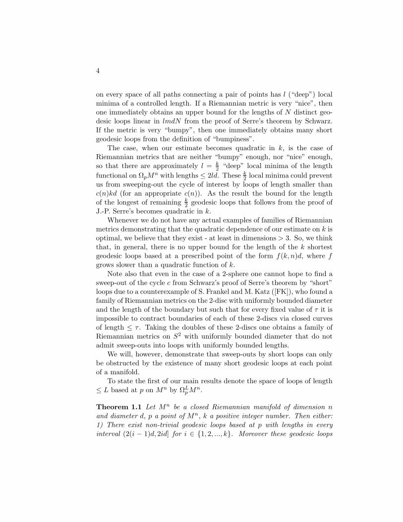
Theorem 1.1 Let Mn be a closed Riemannian manifold of dimension nand diameter d, p a point of Mn, k a positive integer number. Then either:1) There exist non-trivial geodesic loops based at p with lengths in everyinterval (2(i − 1)d, 2id] for i ∈ 1, 2, ..., k. Moreover these geodesic loops

5

are local minima of the length functional on ΩpMn;

or

2) For every positive integer m every map f : Sm −→ ΩpMn is homotopic

to a map g : Sm −→ Ω((4k+2)m+(2k−3))dp Mn. Furthermore, every map f :

(Dm, ∂Dm) −→ (ΩpMn,Ω

((4k+2)m+(2k−3))dp Mn) is homotopic to a map g :

(Dm, ∂Dm) −→ Ω((4k+2)m+(2k−3))dp Mn relative to ∂Dm. In addition, if for

some L the image of f is contained in ΩLp Mn, then the homotopy between

f and g can be chosen so that its image is contained in ΩL+2dp Mn. Also, in

this case for every L every map f from S0 to ΩLp Mn is homotopic to a map

g from S0 to Ω(2k−1)dp Mn by a homotopy such that its image is contained in

ΩL+2dp Mn.

This theorem immediately leads to a quadratic bound for the lengthsof geodesic loops based at p. Indeed, suppose that for some s < k thereare s − 1 non-trivial geodesic loops based at p with lengths in the intervals(0, 2d], (2d, 4d], ..., (2(s − 2)d, 2(s − 1)d], but no geodesic loops based at p oflength in the interval (2(s − 1)d, 2sd]. Then there exists a representationof an even-dimensional cycle c in the loop space that appears in the proofof Serre’s theorem given by A. Schwarz by a spherical cycle that can beformed only by loops of length at most ((8n − 6)s + (4n − 7))d based at p.Thus, we obtain at least s geodesic loops based at p of length ≤ 2(s − 1)d(including the trivial loop), s + 1 loops of length ≤ ((8n − 6)s + (4n − 7))d,s + 2 loops of length ≤ 2((8n − 6)s + (4n − 7))d,..., s + i loops of length≤ i((8n−6)s+(4n−7))d,..., k loops of length ≤ (k−s)((8n−6)s+(4n−7))d.This expression attains its maximum at s = ⌊k

2⌋. The maximal value is((2n− 3

2 )k2 +(2n− 72)k− (1+(−1)k))d. Note that none of the cycles ci from

the prooof of Serre’s theorem by A. Schwarz can “hang” at a local minimumof the length functional on ΩpM

n (at least, unless there is a critical level ofa dimension ≥ dim c but ≤ n − 1 at this local minimum. In such a caseone of the local minima will be “lost” due to the coincidence, but we willimmediately get infinitely many distict geodesics of the same length, whichresults in a much better upper bound for the length.) Therefore wilthoutany loss of generality we can assume that these geodesic loops are distinct.Thus, we are guaranteed to have at least k distinct geodesic loops based at apoint p of length (2n− 3

2)k2 +(2n− 72)k−(1+(−1)k))d (including the trivial

loop). (The new geodesic loops are distinct from each other and from thelocal minima because they have distinct positive indices, when regarded asthe critical points of the length functional.) Thus, one obtains the following

6

theorem in the case when Mn is simply-connected, and p = q:

Theorem 1.2 Let Mn be a closed Riemannian n-dimensional manifold withdiameter d. Then for every point p ∈ Mn there exist at least k distinctgeodesic loops of length at most ((2n−1.5)k2 +(2n−3.5)k− (1+(−1)k))d <2n(k2 + k)d. More generally, for each pair of points p, q ∈ Mn there exist atleast k geodesics starting at p and ending at q of length ≤ ((2n − 1.5)k2 +(2n− 3.5)k)d + (2n− 1.5)kd(p, q), if k is even, and ≤ ((2n− 1.5)k2 + (2n−3.5)k − 2)d + (2n − 1.5)(k + 1)d(p, q), if k is odd. (Here d(p, q) denotes thedistance between p and q in Mn.) In both cases this upper bound does notexceed ((2n − 1.5)k2 + (4n − 5)k + (2n − 3.5))d < 2n(k + 1)2d.

Remark. Denote the smallest odd number l such that there exists a non-trivial rational homotopy class of Mn by l. An elementary rational homotopytheory (cf. [FHT]) implies that l ≤ 2n−1. Our proof of Theorem 1.2 impliesupper bounds ((l − 0.5)k2 + (l − 2.5)k − (1 − (−1)k))d for the lengths of kdistinct geodesic loops based at an arbitrary point p of Mn. Similarly forarbitrary p, q ∈ Mn and arbitrary k there exist at least k distinct geodesicsof length not exceeding ((l − 0.5)k2 + (l − 2.5)k)d + (l − 0.5)kd(p, q), if k iseven, and ((l−0.5)k2 +(l−2.5)k−2)d+(l−0.5)(k+1)dist(p, q), if k is odd.These estimates do not exceed ((l−0.5)k2+(2l−3)k+(l−2.5))d < l(k+1)2d.Also note, that in [NR3] we proved a version of Theorem 1.2 in the casel = 3, but with a worse upper bound that depended factorially on k.

Also, note that 2n(k + 1)2d < 4nk2d for all k ≥ 3, and that we havea better bound 2nd(< 4nk2), when k = 2, proven in [NR1], Therefore,if desired, one can replace the upper bounds for the lengths of k shortestgeodesics between p and q in Mn provided by Theorem 1.2 by a simplerlooking expression 4nk2d.

To prove Theorem 1.2 in the case when Mn is simply-connected, butp 6= q, we prove a generalization of Theorem 1.1, where ΩpM

n is replacedby the space Ωp,qM

n (Theorem 5.3). It immediately yields Theorem 1.2in the case, when p 6= q, exactly as Theorem 1.1 implied the case p = q.

To obtain Theorem 1.2 in the nonsimply-connected case we will con-sider the universal covering of Mn constructed from the space of all pathsstarting at p via the standard identification and endowed with the pull backRiemannian metric. According to the standard argument that can be foundin many textbooks on Riemannian geometry one can choose the fundamen-tal domains in the universal covering so that their interiors are all isometricto the complement of the cut locus of the base point p, and, therefore, their

7

diameter does not exceed 2d. If the cardinality of π1(Mn) is infinite or finite

but ≥ k, we will connect the base point p in the universal covering Mn

of Mn with k closest liftings of q by shortest geodesics. The projectionsof these geodesics to Mn will have lengths ≤ (2k − 1)d, and the theoremfollows. If the cardinality of π1(M

n) is less than k, then we observe thatMn is a simply-connected manifold of diameter d ≤ 2|π1(M

n)|d (as the di-ameter of each fundamental domain does not exceed 2d). Let ks denote thesmallest integer number which is not less than k

|π1(Mn)| . We are going toconnect p with each lifting of q by ks or ks − 1 distinct geodesics, so as toobtain the required number k of distinct geodesics between p and q afterprojecting down to Mn. (Obviously, if we need to connect p with somepoints in the lifting of q to Mn with ks geodesics, and with some otherpoints in the lifting of q with ks − 1 geodesics, we choose points that weconnect with p by ks geodesics to be the points that are the closest to p.)If one knows how to prove Theorem 1.2 in the simply-connected case, thenone can get a slightly worse upper bound (but still with the leading term

2|π1(Mn)|(2n − 1.5)k2d ≤ (2n − 1.5)k2d) in the nonsimply-connected case.

(Indeed, asymptotically k2 will be divided by |π1(Mn)|2 , and multiplied by

2|π1(Mn)|.) To prove a better upper bound we will need the following:

Theorem 1.3 Let M be a closed Riemannian manifold of diameter d with afinite fundamental group of cardinality C. The the diameter of the universalcovering space M of M endowed with the pull back Riemannian metric doesnot exceed Cd.

It is hard to believe that Theorem 1.3 is not known, yet we were notable to find any mention of it in the literature. Therefore we will prove itin Section 6 of this paper. There we will also present a proof the followinggeneralization of Theorem 1.3:

Theorem 1.4 If the fundamental group of a closed Riemannian manifoldM of diameter d is either infinite or finite of order ≥ k, then for every pairof points p, q ∈ M and every k there exist at least k geodesics connecting pand q of length ≤ kd that represent different path homotopy classes.

We can combine Theorem 1.3 with the described simple procedure thatallows one to reduce Theorem 1.2 for a nonsimply-connected Mn to Theo-rem 1.2 for its universal covering Mn. As the result, we obtain upper boundsfor the nonsimply-connected case that are not worse than the estimates inthe simply-connected case. As it was already mentioned, the verification

8

mostly involves checking of what happens for small values of k. We arenot going to present the details of the straightforward and elementary buttedious calculations here.

The proof of Theorem 1.1 is based on a new curve shortening process.This process will be introduced in the proof of the following theorem atthe beginning of section 3. Before stating this theorem recall that a pathhomotopy between two curves β and γ is a homotopy that preserves theend points. In other words, it is a family of curves ατ (t) that continuouslydepends on τ ∈ [0, 1] such that α0 = β, α1 = γ, and such that for everyτ ∈ [0, 1] ατ (0) = α0(0) and ατ (1) = α0(1).

Theorem 1.5 Let Mn be a closed Riemannian manifold of diameter d, andp, q be two arbitrary points of Mn. Let γ(t) be a curve of length L connectingpoints p and q. Assume that there exists an interval (l, l + 2d], such thatthere are no geodesic loops based at p on Mn of length in this interval thatprovide a local minimum of the length functional on ΩpM

n. Then thereexists a curve γ(t) of length ≤ l+d connecting p and q and a path homotopybetween γ and γ such that the lengths of all curves in this path homotopy donot exceed L + 2d.

Observe that this theorem immediately implies Theorem 1.1 for m = 0.Indeed, S0 consists of two points, so , if m = 0, then f is just a set of twoloops. In the absence of k short geodesic loops providing local minima forthe length functional each of these two loops can be shortened as in Theorem1.5.

The statement of Theorem 1.1 can be interpreted as a parametric versionof Theorem 1.5. Yet note that the curve-shortening process that will beused to prove Theorem 1.5 does not depend on γ continuously, and there isno obvious way to obtain a desired parametric version. The best that onecan do is to choose a sufficiently dense finite set of loops Li in f(Sm) andto shorten them as in Theorem 1.5. Indeed, we will do that in the courseof proving Theorem 1.1. But this will leave us with all the other loopsin between that still remain long. The further idea can be very vaguelydescribed as follows. In the process of shortening loops Li we will createcontinuous 1-dimensional families of paths of controlled length (“rails”) thatconnect p with all points on Li. The image of g(Sm) in Mn will be the unionof the image of f(Sm) in Mn and the constructed “rails”. (Recall that eachpoint of f(Sm) is a loop in Mn; here we are talking about the union of allthese loops.) The image of f(Sm) in Mn will be cut into very short arcs

9

starting and ending on curves Li. These short arcs form an m-dimensionalfamily A. Each of these arcs from family A will be included into a loop fromthe family g(Sm). Every loop from g(Sm) will contain only a controllednumber of arcs from A, so their total contribution to the length of the loopis negligibly small. Besides arcs from A each loop from g(Sm) will alsocontain a controlled number of “rails” and arcs of the curves Li, so that itstotal length will be under control.

Now we would like to give a brief review of some existing results relatedto Theorem 1.2. The first curvature-free upper bounds for the length of ashortest non-trivial geodesic loop on a closed Riemannian manifold in termsof either diameter or the volume of the manifold were proven by S. Sabourauin [S]. However, Sabourau considered the situation when the minimization ofthe length of the geodesic loop was performed also over all possible choicesof the base point of the loop. R. Rotman ([R]) demonstrated that for everypoint p on every closed n-dimensional manifold of diameter d the lengthof the shortest geodesic loop based at p does not exceed 2nd. (It is easyto see that if the base point is prescribed, then there is no upper boundfor the length of the shortest geodesic loop in terms of the volume of themanifold, even if the manifold is diffeomorphic to the 2-sphere.) Note alsothat a shortest non-trivial geodesic loop based at p is the second shortestgeodesic starting and ending at p. In [NR1] it was proven that the sameestimate 2nd holds for the length of the second shortest geodesic between twoarbitrary points p and q of an arbitrary n-dimensional Riemannian manifoldof diameter d. This is the best known upper bound in the case, when k = 2(for every simply-connected manifold Mn).

If n = 2, one can also produce better estimates than the estimates pro-vided by Theorem 1.2. In [NR2] we proved that if n = 2 and Mn isdiffeomorphic to the 2-sphere , then two arbitrary points can be connectedby at least k distinct geodesics of length ≤ (4k2−2k−1)d. (In the same pa-per we have also shown that this estimate can be improved to 4k2 − 6k + 2if these points coincide). Making an almost obvious observation that thecycles corresponding to powers of u from the proof of A. Schwarz do not“hang” on local minima of the length functional and, therefore, geodesicscorresponding to cup powers of u are different from the geodesics that arelocal minima of the length functional, we can immediately improve theseupper bounds for k > 2 to (k2 +3k +3)d in the case of geodesics connectingtwo distinct points of M2 and (k2 + k)d in the case of geodesic loops basedat any prsecribed points of M2. (One of these (k2 + k)d geodesic loops canbe trivial.) The simple argument used above to reduce Theorem 1.2 in the

10

non-simply conected case to its simply-connected version (for the univeralcovering) can be combined with these estimates for S2 to deduce the sameupper bounds (k2 + k)d for the lengths of k shortest geodesic loop based ata prescribed point of M2 and (k2 + 3k + 3)d for the lengths of k shortestgeodesics connecting every prescribed pair of points of M2 in the case, whenM2 is diffeomorphic to RP 2. Note that Theorem 1.4 yields even betterupper bounds (namely, kd), in the case, when a closed two-dimensional Rie-mannian manifold M2 is not diffeomorphic to S2 or RP 2. Thus, Theorem1.2 should only be used in the case when n, k ≥ 3 (and |π1(M

n)| is finiteand “small”).

In section 7 we will discuss generalizations of Theorems 1.1, 1.5 and 5.3that involve the notion of the depth of local minima of the length functional.The formal definition of the depth will be given in section 7. Informally, thedepth of a non-trivial local minimum γ of the length functional on ΩpM

n

is the difference between the maximal length of a loop during an “optimal”path homotopy contracting γ and the length of γ.

First, we observe that Theorem 1.5 remains valid if instead of assumingthat there are no local minima of the length functional with length in theinterval (l, l + 2d] we assume that there are no local minima of depth ≥ 2dwith the length in this interval. As a corollary, one can strengthen Theorem1.1 by requiring in the first case that the geodesic loops with lengths in theintervals (2(i − 1)d, 2id] are not only local minima of the length functional,but local minima of depth ≥ 2d. Then we generalize this stronger versionof Theorem 1.1 (as well as of Theorem 5.3) by requiring in the first casethat the depth of these local minima is not only ≥ 2d but ≥ S for someS ≥ 2d. The “price” is a corresponding increase of the lengths of the loopsthat must appear in the second case that is proportional to S − 2d.

We finish section 7 by observing that for a specific sufficiently large valueof S the first case in Theorem 1.1 cannot occur already for k = 1, and thegeneralized form of the second case holds unconditionally.

As the result, we obtain a different proof of a well-known theorem firstproven by M. Gromov (see section 1.4 in [Gr0] or ch. 7 in [Gr]) that assertsthat for every simply-connected closed Riemannian manifold Mn there existsa constant C such that for every m the inclusion ΩCm

p Mn ⊂ ΩpMn induces

the surjective homomorphisms of homotopy groups in all dimensions up tom. Our proof yields a good estimate for the constant C that seems to bebetter than the value that one can extract from the proof by Gromov. Thecomparison between our results and the results by M. Gromov is done inthe last section of the paper.

11

2 A simple lemma and its multidimensional gen-

eralization.

The proof of 1.5 uses the following known lemma. To state this lemma weare going to introduce the following notations that we will be widely usingfurther below in this paper. Let τ(t) be a path in Mn. We are going todenote the “same” path travelled in the opposite direction as τ . If a is apath from x to y, and b is a path from y to z, then we will denote by a ∗ bthe join of a and b, that is the path from x to z that first follows a from xto y, and then b from y to z. Observe, that if e1, e2 are two paths from p toq, then e1 ∗ e2 is a loop based at p.

Lemma 2.1 Let e1, e2 be two paths starting at q1 and ending at q2 on acomplete Riemannian manifold Mn. Denote the length of ei, i = 1, 2, by li.

If the loop α0 = e1∗e2 can be connected to a (possibly trivial) loop α = α1,(see fig. 1 (a)), by a path homotopy that passes via loops ατ , τ ∈ [0, 1],of length ≤ l1 + l2, then there is a path homotopy hτ (t), τ ∈ [0, 1], suchthat h0(t) = e1(t), h1(t) = α ∗ e2(t) and the length of the paths during thishomotopy is bounded above by l1 + 2l2.

Proof. For the proof see fig. 1. Note that e1 is path homotopic to e1∗ e2∗e2

along the curves of length ≤ l1 +2l2 , see fig. 1 (b,c). (We just insert longerand longer segments of e2 travelled twice in the opposite directions.) Nowobserve that as e1 ∗ e2 is path homotopic to α via the curves ατ of length≤ l1 + l2, the path e1 ∗ e2 ∗ e2 is path homotopic to α ∗ e2 along the curvesατ ∗ e2 of length at most l1 + 2l2, see fig. 1 (d,e). 2

Note that the above lemma has the following higher-dimensional gen-eralization: Let f : Sm −→ ΩL

q1,q2Mn, i = 1, 2, m ≥ 1, be a continuous

map from the m-sphere into a space of (piecewise differentiable) paths ona complete Riemannian manifold Mn between points q1, q2 ∈ Mn of lengthat most L. Let L0 = mins∈Sm length(f(s)), and s0 ∈ Sm be such thatlength(f(s0)) = L0. One can define a new map F : Sm −→ ΩL+L0

q1Mn

by the formula F (s) = f(s) ∗ f(s0). Assume that there exists a homotopyFt : Sm −→ ΩL+L0

q1Mn contracting F . (Here t ∈ [0, 1], F0 = F,F1 is the

constant map to the trivial loop based at q1.) Then we have the followingsimple lemma:

Lemma 2.2 There exists a homotopy ft : Sm −→ ΩL+2L0

q1q2Mn, t ∈ [0, 1],

between f = f0 and the constant map f1 of Sm identically equal to f(s0).

12

e1e2

q1

q2

e1

q1

q2

α e2

e1

q1

q2

e1

q1

q2

e1 e2e2* − *

e2

q1

q2

α τ

α τ * e2

e2

q1

q2

α

α * e2

a b c d e f

Figure 1: Illustration of the proof of Lemma 2.1.

Proof. First note that the main point of the lemma is that for every t ft

takes values in the space of paths of length ≤ L+ 2L0 connecting q1 and q2.The desired homotopy is constructed in two stages. During the first stagewe connect f with f 1

2

defined by the formula f 1

2

(s) = f(s) ∗ f(s0) ∗ f(s0) =

F (s) ∗ f(s0). At this stage we join f(s) with longer and longer segments off(s0) travelled twice with opposite orientations.

During the second stage we contract F using the homotopy Ft, t ∈ [0, 1]leaving intact f(s0) at the end of each loop Ft(s) ∗ f(s0). 2

In the next section we will present a proof of Theorem 1.5.

3 Curve-shortening process in the absence of geo-

desic loops.

Proof of Theorem 1.5.

l+ d+ δ

p q

Figure 2: Curve shortening process (i).

Assume that there are no geodesic loops based at p with the length inthe interval (l, l + 2d]. Using an obvious compactness argument we observe

13

that there exists a positive δ0 such that there are no geodesic loops based atp with the length in the interval (l, l+2d+δ0]. Obviously, one can choose thevalue of δ0 to be arbitrarily small, if desired. Without any loss of generalitywe can assume that the length L of the curve γ : [0, L] −→ Mn parametrizedby its arclength is greater than l + d. Let δ = δ0, if L ≥ l + d + δ0, andδ = L− l− d, if δ ∈ (l + d, l + d + δ0). Consider the segment γ|[0,l+d+δ] of γ,which we will denote γ11(t) and the segment γ|[l+d+δ,L] denoted γ12(t) (seefig. 2).

l+d+δ

the length of e is at most d1

qp

Figure 3: Curve shortening process (ii).

Let us connect points p and γ(l + d + δ) by a minimal geodesic, e1 (oflength ≤ d), (see fig. 3). Then the pair of curves γ11 and e1 form a loopγ11 ∗ e1 of length ≤ l + 2d + δ based at p.

the length of the loop is at most l

l+d+ δp q

Figure 4: Curve shortening process (iii).

Consider a (possibly trivial) shortest loop α1 that can be connected withγ11∗e1 by a length non-increasing path homotopy. (Its existence follows fromthe Ascoli-Arzela theorem.) Obviously, α1 is a geodesic loop based at p thatprovides a local minimum for the length functional on ΩpM

n. Therefore ourassumptions imply that the length of α1 is at most l.

By Lemma 2.1 γ11 is path homotopic to the curve α1 ∗ e1 = γ11 alongthe curves of length at most l + 3d + δ and, thus, the original curve γ ishomotopic to a new curve γ11 ∗γ12 along the curves of length at most L+2d,(see 5).

14

p ql+d+δ

Figure 5: Curve shortening process (iv).

Note that the length L1 of this new curve γ1 = γ11 ∗ γ12 is at mostL − δ. Assuming that L1 is still greater than l + d, we repeat the processagain: We parametrize γ1 by its arclength. Now, let γ21 = γ1|[0,l+d+δ] andγ22 = γ1|[l+d+δ,L1]. (Here, as before, if L1 < l + d+ δ, then we use L1 − l− das the new value of δ, but otherwise keep the old value of δ = δ0.)

the length of e is at most d2

l+d+δqp

Figure 6: Curve shortening process (v).

Connect the points p and γ1(l + d + δ) by a minimal geodesic segmente2, (see fig. 6). Then γ21 and e2 form a geodesic loop γ21 ∗ e2 based at p oflength at most l + 2d + δ.

Again, we try to connect this loop with a shortest possible loop α2 bymeans of a length non-increasing path homotopy. The existence of a mini-mizer α2 follows from an easy compactness argument, and α2 is a geodesicloop providing a local minimum of the length functional on ΩpM

n, (see fig.7). Therefore, the length of α2 is at most l.

Thus, γ21 is path-homotopic to γ21 = α2 ∗ σ2 along the curves of lengthat most l + 3d + δ. It follows that γ1 is homotopic to γ2 = γ21 ∗ γ22 alongthe curves of length at most L + 2d, (see fig. 8).

We will continue this process in the same manner. It is obvious thatthis process will terminate in a finite number of steps with a curve of length≤ l + d, and that the number of steps will not exceed ⌊L−l−d

δ0⌊+1 . 2

15

l+d+δ

the length of e is at most d2

the length of the new loop is still at most l

p q

Figure 7: Curve shortening process (vi).

l+d+δp q

Figure 8: Curve shortening process (vii).

the length of this curve is at most l+d

p q

Figure 9: Curve shortening process (viii)

16

Note that we have proven a stronger statement. We have shown, assum-ing the hypothesis of the theorem above, that for each path γ(t) connectingp and q there exists a 1-parameter family of curves Cγ

s of length ≤ l+3d+ δcontinuously depending on a parameter s that connects p with all points ofγ(t), so that:

A. If we denote Cγs (1) by γ(τ(s)), then τ(s) is an increasing (but, in general,

not strictly increasing) function of s;

B. There exist two partitions: P γ = 0 = tγ0 < tγ1 < tγ2 < ... < tγkγ = 1 andQγ = 0 = sγ

0 < sγ1 < ... < sγ

2kγ = 1, such that

(1) Cγs (1) = γ(tγi ) for s ∈ [sγ

2i−1, sγ2i].

(2) Cγs (1) = γ(r) for r ∈ [rγ

i , rγi+1] and s ∈ [sγ

2i, sγ2i+1].

(3) For all i the length of Cγ

sγ2i

does not exceed l + d.

(4) The curve Cγ

sγ

2kγ= Cγ

1 is the final result of the application of the curve-

shortening process described in the proof of Theorem 1.5 to γ.

The curves Cγs are depicted on Fig. 6-10 as the curves connecting p with

a variable point that moves from p to q along γ. Note also, that the partitionP γ can be chosen as fine as desired.

Finally, notice that the constructed path homotopy H between our orig-inal path, γ, and Cγ

1 can be described as follows: At each moment of time tH(t) is the path that first goes along Cγ

t , and then runs along γ from Cγt (1)

to γ(1).

Next we will prove the following theorem, which together with Theorem1.5 immediately implies Theorem 1.1 in the case of m = 1.

Theorem 3.1 Let Mn be a closed Riemannian manifold of diameter d, pa point of Mn, and k a positive integer number. Assume that there existsa positive integer j ≤ k such that the length of every geodesic loop thatprovides a local minimum for the length functional on ΩpM

n is not in theinterval (2(j − 1)d, 2jd]. Consider a continuous map f : [0, 1] −→ ΩpM

n

such that the lengths of both f(0) and f(1) do not exceed 2(j − 1)d. Then

f is path homotopic to f : [0, 1] −→ Ω(6j−1)dp Mn ⊂ Ω

(6k−1)dp Mn. Moreover,

assume that for some L the image of f is contained in ΩLp Mn. Then one

can choose a path homotopy between f and f so that its image is containedin ΩL+2d

p Mn.

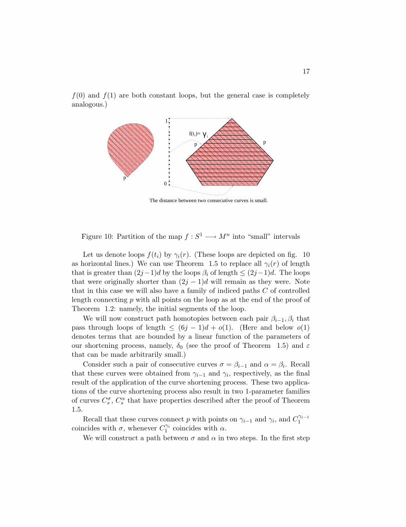
Proof. Choose a partition of t0 = 0 < t1 < t2 < ... < tN = 1 of the interval[0, 1], so that maxi maxτ∈[0,1] length(f(t)|t∈[ti−1,ti](τ)) ≤ ε for a small ε thatwill eventually approach 0, (see fig. 10. Fig. 10 depicts a situation, when

17

f(0) and f(1) are both constant loops, but the general case is completelyanalogous.)

p p

0

1

f(t )i γ i=

p

The distance between two consecutive curves is small.

Figure 10: Partition of the map f : S1 −→ Mn into “small” intervals

Let us denote loops f(ti) by γi(r). (These loops are depicted on fig. 10as horizontal lines.) We can use Theorem 1.5 to replace all γi(r) of lengththat is greater than (2j−1)d by the loops βi of length ≤ (2j−1)d. The loopsthat were originally shorter than (2j − 1)d will remain as they were. Notethat in this case we will also have a family of indiced paths C of controlledlength connecting p with all points on the loop as at the end of the proof ofTheorem 1.2: namely, the initial segments of the loop.

We will now construct path homotopies between each pair βi−1, βi thatpass through loops of length ≤ (6j − 1)d + o(1). (Here and below o(1)denotes terms that are bounded by a linear function of the parameters ofour shortening process, namely, δ0 (see the proof of Theorem 1.5) and εthat can be made arbitrarily small.)

Consider such a pair of consecutive curves σ = βi−1 and α = βi. Recallthat these curves were obtained from γi−1 and γi, respectively, as the finalresult of the application of the curve shortening process. These two applica-tions of the curve shortening process also result in two 1-parameter familiesof curves Cσ

s , Cαs that have properties described after the proof of Theorem

1.5.

Recall that these curves connect p with points on γi−1 and γi, and Cγi−1

1

coincides with σ, whenever Cγi

1 coincides with α.

We will construct a path between σ and α in two steps. In the first step

18

we will consider a loop that is a join of σ and α, namely, σ ∗ α. We willconstruct a homotopy that contracts this loop to a point via loops of length ≤4jd+o(1) (when δ+ε0 −→ 0). The second step will be merely an applicationof Lemma 2.1. (On the second step the summand of 2(j−1)d+d = (2j−1)dwill be added to the previous upper bound 4jd+ o(1) for the length of loopsduring the contracting homotopy.) The desired estimate (6j − 1)d can beobtained by passing to the limit as ε + δ0 −→ 0.

So, we need only to describe the first step to finish our construction.Note that γi−1 and γi are very close to each other, and are connectedby the continuous family of very short curves f(t)|t∈[ti−1,ti](τ), τ ∈ [0, 1].The desired continuous family of loops could be described as the family ofall loops C

γi−1

s1∗ f(t)|t∈[ti−1,ti](τ) ∗ Cγi

s2, where C

γi−1

s1(1) = f(ti−1)(τ) and

Cγis2

(1) = f(ti)(τ) but otherwise s1, s2 and τ independently vary over [0, 1]interval. It is easy to see that these loops form a continuous one-parametricfamily that can be naturally parametrized by an interval of length not ex-ceeding 2. Yet observe that whole intervals of values of s1 and/or s2 couldcorrespond to some individual values of τ . We have some freedom on howwe parametrize this family. We would prefer to parametrize them in a slowerway than possible to somewhat improve the bounds on the lengths of theseloops. Observe, that some of the curves C have better upper bounds fortheir length. The reason is that the length of the curves during each pathhomotopy that shortens the length by δ as described in the proof of Theo-rem 1.5 could increase up to 2d in comparison with the length of the curveat the end of the considered step (and up to 2d + δ in comparison with thelength of the curve at the beginning of this step). Therefore, we do not wantto make these homotopies in families Cγi−1 and Cγi simultaneously, but willwait until one of these homotopies ends, and then perform the other.

Here is a more concrete description of the resulting one-parametric familyof loops that also takes into account some details of the construction of Cγ

s

in the proof of Theorem 1.5 above.

Let ετ = f(t)(τ), where τ is fixed and t varies in the interval [ti−1, ti].Recall that we can ensure that the length of ετ is arbitrarily small for allτ ∈ [0, 1] by choosing ti − ti−1 to be sufficiently small.

Let us begin with the loop σ ∗ α = Cσ1 ∗ Cα

1 that is based at the pointp. Corresponding to Cσ

s and Cαs consider two pairs of partitions: P σ , Qσ

and Pα, Qα. Let P σ = 0 = rσ0 < rσ

1 < ... < rσkσ−1 < rσ

kσ= 1 and

Pα = 0 = rα0 < rα

1 < ... < rαkα−1 < rα

kα. Also let P = P σ ∪ Pα. Without

any loss of generality, we can assume that P = 0 = rσ0 = rα

0 < rα1 < rσ

1 <

19

rα2 < rσ

2 < ... < rαkα−1 < rσ

kσ−1 < rαkα

= rσkσ

= 1.

We will now present a homotopy that contracts σ ∗ α to p as a loop overshort loops.

(a) Cσ1 ∗ Cα

1 is homotopic to Cσsσ2kσ−1

∗ Cα1 over loops of length at most 4jd,

see fig. 11.

p

p p

Csσ

2k σCs

σ

2k σ−1

p

homotopic to

Figure 11: Contracting σ ∗ α as a loop (i).

(b) Cσsσ2kσ−1

∗Cα1 is homotopic Cσ

sσ2kσ−1

∗Cαsα2kα−1

over the loops of length 4jd,

(see fig. 12).

p

Csσ

2k σ−1

Cαs2k α

α

Cαs

2k −1αα

p p

p

homotopic to

σ

Figure 12: Contracting σ ∗ α as a loop (ii).

20

(c)Cσsσ2kσ−1

∗Cαsα2kα−1

is homotopic to Cσsσ2kσ−2

∗εrσk−1

∗Cαsα for sα ∈ [sα

2k−2, sα2k−1]

over the curves of length at most (4j − 2)d + 2δ + ε, (see fig. 13).

p

p

Cαs

2k −1αα

p

Csσ

2k σ−1σ

Csσ

2kσ

σ −2

homotopic to

Figure 13: Contracting σ ∗ α as a loop (iii).

(d) Cσsσ2kσ−2

∗ εrσk−1

∗ Cαsα is homotopic to Cσ

sσ2kσ−3

∗ εrσk−1

∗ Cαsα over the curves

of length 4jd + 2δ + ε, (see fig. 14).(e) Cσ

sσ2kσ−3

∗ εrσk−1

∗ Cαsα is homotopic to Cσ

sσ ∗ εrαk−1

∗ Cαsα2kα−2

for sσ ∈

[sσ2kσ−3, s

σ2kσ−4] over the curves of length at most (4j − 2)d + 2δ + ε, (see fig.

15).Proceeding in the above manner we will contract the loop to p over

curves of length at most 4jd + o(1).Observe that after an appropriate reparametrization of all families Cγi

s

by s (a “synchronization”) all the constructed loops have the form Cγi−1

s ∗f(t)|t∈[ti−1,ti](τ(s)) ∗ ¯C

γi−1

s for an appropriate increasing but not necessarilystrictly increasing function τ(s). It is easy to see that one can choose thesesynchronizations so that the same parametrization of the family Cγi willwork for constructions of path homotopies between βi−1 and βi and betweenβi and βi+1. Observe, that for every s the length of one of two curves C

γi−1

s

and Cγis does not exceed (2j − 2)d + d + o(1) = (2j − 1)d + o(1), and the

length of the other does not exceed (2j − 1)d + o(1) + 2d = (2j + 1)d + o(1),as δ −→ 0. Combining the constructed path homotopies between βi−1 andβi for all i we obtain a path in ΩpM

n starting at f(0) and ending at f(1),

21

Csσ

2kσ

σ −2

p p

p σCsσ

2k σ−3

homotopic to

Figure 14: Contracting σ ∗ α as a loop (iv).

p

p

Cs2k

αα

α

p

Cs2k −2

αα

α

−1

homotopic to

Figure 15: Contracting σ ∗ α as a loop (v).

22

which can be interpreted as a map of [0, 1] into ΩpMn.

It remains to prove that this path f in ΩpMn is path homotopic to f .

Here is the construction of a path homotopy between f and f : At eachmoment of time we do not shorten f(ti) (for all i) all the way using theconstruction in the proof of Theorem 1.5, as we did above. Instead weuse a partial shortening described after the proof of Theorem 1.5 in theconstruction of the homotopy H. We denote these homotopies H betweenγi and its shortening by Hi. For every λ ∈ [0, 1] the path Hi(λ) consists oftwo arcs. The first arc is the path Cγi

λ (where the parametrization of the one-parametric family Cγi

s is the same as the one that has been used to constructcontractions of βi−1 ∗ βj and βj ∗ ¯βj+1 above). The second arc is the arc ofγi that starts at C

γj

λ (1) and ends at the end of γj. To construct the desiredpath homotopy between f and f in ΩpM

n at the moment λ we replaceall long curves γi not by βi = Hi(1) but by Hi(λ). As we synchronized theparametrizations of different one-parametric families C, Cγi

s (1) and Cγi−1

s (1)can be connected by a (very short) arc f(t)|t∈[ti−1,ti](τ) for a fixed value ofτ = τ(s). Now we can form loops Cγi

r ∗ f(t)|t∈[ti−1,ti](τ(r)) ∗ Crγi−1 for all

r ≤ λ, as it was done above. These loops provide a contracting homotopyfor the loop Cγi

λ ∗ f(t)|t∈[ti−1,ti](τ(λ)) ∗ Cλγi−1 . Using Lemma 2.1 we can

transform this homotopy into a path homotopy between Cγi−1

λ and Cγi

λ ∗f(t)|t∈[ti−1,ti](τ(λ)). Joining all paths in this path homotopy with the arc

γλi−1 of γi−1 between C

γi−1

s (1) and γi−1(1) = p , we obtain a path homotopybetween Hi−1(λ) and Cγi

λ ∗f(t)|t∈[ti−1,ti](τ(λ))∗γλi−1 . It remains to construct

a path homotopy between f(t)|t∈[ti−1,ti](τ(λ)) ∗ γλi−1 and γλ

i . But that pathhomotopy can be formed by paths f(t)|t∈[,ti](τ(λ)) ∗ f(, τ), τ ∈ [τ(λ), 1],parametrized by τ , where is the parameter of the path homotopy, ( ∈[ti−1, ti]). Combining these short paths connecting Hi−1(λ) and Hi(λ) forall i we obtain fλ, where f0 is f , and f1 is f .

It is easy to see from this description that the resulting path homotopypasses through paths of length ≤ L + 2d. (The increase of length alreadytakes place during the first stage, when we shorten curves γi using Theorem1.5. If L ≤ (6k−1)d, we can just take f = f , so without any loss of generalitywe can assume that L > (6k − 1)d. It is easy to see that in this case thejust described path homotopy between Hi−1(λ) and Hi(λ), λ ∈ [0, 1] doesnot lead to any further increase of the lengths of paths.)

We would like to provide the following less formal explanation (or rein-terpretation) of the construction of the path homotopy between Hi−1(λ) andHi(λ). These two paths consist of curves C

γi−1

λ and Cγi

λ joined with nearly

23

identical “tails” that are the arcs of γi−1(τ) and γi(τ) between τ = τ(λ)and τ = 1. The “tails” form a part of one parametric family of “tails”f(, τ), τ ∈ [τ(λ), 1], where the parameter ranges in [ti−1, ti]. The ideawas to “fill” the “digon” formed C

γi−1

λ and Cγi

λ in exactly the same way aswe filled the digon formed by βi−1 = C

γi−1

1 and βi = Cγi

1 by a one-parametricfamily of paths of controlled length, and to attach to each of these paths thecorresponding “tail” f(, τ), τ ∈ [τ(λ), 1], for an appropriate value of . Ofcourse, this idea requires some minor corrections as 1) C

γi−1

λ and Cγi

λ endat very close but still different points, and will form a digon only after weattach (a very short) path f(t)|t∈[ti−1,ti](τ(λ)) connecting their endpoints toone of them; 2) We will be able to attach an appropriate “tail” f(, τ) onlyafter attaching (a very short) arc of f(t)|t∈[ti−1,ti](τ(λ)). But, as we will seebelow, this idea directly generalizes to situation, when one deals with mapsof higher dimensional spheres to ΩpM

n.2

Remark 3.1. Here we would like to summarize some important featuresof our construction of f that will be used to prove Theorem 1.5 for largervalues of m. The constructed homotopies contracting βi−1 ∗ βi that were themain part of the construction of f in the proof of Theorem 3.1 consist ofloops containing the images of rectilinear arcs [ti−1, ti] × τ for a variableτ ∈ [0, 1] that monotonously depends on the parameter of the homotopy.The loops can be naturally diveded into two arcs, such that the length ofone of these arcs does not exceed (2j−1)d+o(1), and the length of the otherdoes not exceed (2j + 1) + o(1), as δ, ε −→ 0. The path homotopy betweenβi−1 and βi is obtained from the path homotopy contracting βi−1 ∗ βi bysimply applying (the construction in the proof of) Lemma 2.1. The desiredmap f was constructed by combining the path homotopies between βi−1 andβi for all i.

4 Small spheres in the loop space.

In this section we will demonstrate that in the absence of a great number ofshort geodesic loops, every homotopy class of ΩpM

n can be represented bya sphere that passes through short loops (thus proving Theorem 1.1). Weassume that there exists k such that there are no geodesic loops based at p onMn with the length in the interval (2(k−1)d, 2kd] providing a local minimumfor the length functional. We are going to prove that f is homotopic to amap g with the image in ΩL

p Mn, where L = ((4k + 2)m + (2k − 3))d.

24

The proof of the theorem is done by induction on m. The base step ofthe induction, (m = 1), had been proven in the previous section. Beforepresenting the proof of the induction step, we would like to explain how theproof will work to pass from m = 1 to m = 2. (We will explain the proof inthe case, when f is a map of S2. It will be clear from our explanations thatthe case, when f is a map of the pair (D2, ∂D2) can be treated exactly thesame.)

I Ix

Rij

p

p

p

p

p

p

p

p

0−skeleton 1−skeleton 2−skeleton

(a) (b) (d)(c)

Figure 16: Replacing the map

Let I = [0, 1]. Consider a map f : I × I −→ ΩpMn, where

∂(I × I) is mapped to p. Let us subdivide I × I into small squares,of size that will be specified later. Consider a square Rij with vertices(xi−1, yj−1), (xi−1, yj), (xi, yj−1), (xi, yj). Each of these vertices correspondsto a loop in ΩpM

n. Each of these loops that is too long, (i.e. of lengthgreater than (2k− 1)d) will be replaced by a shorter one as in Theorem 1.5via a path homotopy described in the proof of Theorem 1.5. Now, we willreplace the edges that connect these vertices as in the proof of Theorem 3.1in the previous section (see fig. 16 (a)-(c)). Next, we have to “fill” the

25

interior of the square, (fig. 16 (d)).

The boundary of this square corresponds to a 2-sphere in Mn. It isconvenient to consider it as a CW-complex with the following sturcture: aboundary of a parallelipiped in which two opposite faces have been collapsedto a point and identified with the point p, (see 17). Note that the two copiesof p at the beginning and the end of considered loops will be sometimesdepicted on our figures as two different points (fig. 17). This convention willmake our figures easier to draw and comprehend, and will also make clearerthe fact that our proof can be easily adapted to prove the generalization ofthe theorem, where ΩpM

n in the conclusion of the theorem is replaced byΩpqM

n for two arbitrary points p, q.

p

p

Figure 17: Sphere decomposition.

Each of the four “large” cells of the sphere has a natural decompositioninto “short” loops based at p. (Here “short” means of length at most 4kd +o(1); recall the proof of Theorem 3.1 in the previouos section).

The filling will be done in four steps.

Step 1. We will construct a homotopy between the sphere and the pointp, such that for every τ ∈ [0, 1] the (map of the) sphere S2

τ in the homotopywill have a similar decomposition into short loops based at p. This meansthat each sphere S2

τ will be given a CW-structure of the cell complex of the

26

boundary of a parallelipiped in which two opposite faces are mapped intop and into another point depending on τ and denoted q(τ), respectively,and where each of the remaining four (“large”) faces are swept-out by loopsof length at most 4kd + o(1) based at p. We will be using the proof ofTheorem 3.1 and, in particular, the facts summarized in Remark 3.1 to dothis construction.

Step 2. For each τ we can construct a vertical sweep-out of S2τ by curves of

length of at most (6k+1)d+o(1), which will vary continuously with respectto τ . Here by the vertical sweep-out we mean a continuous 1-parametricfamily of curves joining a pair p, qτ of points of S2

τ . In fact, this family canbe parametrized by a circle. This step essentially consists in an application ofLemma 2.1 to each of four “large” faces of S2

τ . The resulting path homotopyfor each face corresponds to one quarter of the circle parametrizing the wholefamily.

Step 3. Each of these paths can be paired with a fixed path of length≤ (2k+1)d+o(1) to obtain a sweep-out of each sphere Sτ

2 by loops of length

≤ (8k+2)d+o(1). This path is the join of Cf(v)τ (from the proof of Theorem

1.5, where v denotes an arbitrary vertex of the considered rectangle Rij)with a very short segment connecting its endpoint with qτ in the image ofRij × τ. But for reasons of continuity one needs to consider the samevertex v for all values of τ . (It might seem that we could ensure a somewhatsmaller length of the loops: For every value of τ we could find a vertex v

(that would depend on τ) such that Cf(v)τ has length ≤ (2k − 1)d + o(1).

But in this case the resulting circle in ΩpMn representing S2

τ does not needto depend continuously on τ , and is not suitable for our purposes.)

Step 4. We can now apply Lemma 2.2 to obtain a 3-disc filling the original2-sphere, S2

1 , and so that this 3-disc is swept-out by paths connecting p andq1 = p of length at most (8k + 2)d + (2k − 1)d + o(1) = (10k + 1)d + o(1).

This completes the construction of the filling of ∂Rij × [0, 1] for onesmall square Rij. Combining these fillings for all values of i, j we obtaina map F : S3 −→ Mn with a vertical sweep-out (by paths connecting pand q1 = p, that is, by loops based at p) of a controlled length, which, inturn, can be reinterpreted as a map f : S2 −→ ΩpM

n with the image in

Ω(10k+1)d+o(1)p Mn.

Note that the only step in this construction which is not immediateand requires a more detailed description is the first one. We will thereforedescribe it in more details than the other three steps. Let us once againconsider a map f |Rij

. It induces a map F : Rij × [0, 1] −→ Mn defined by

27

the formula F (x, y, t) = f(x, y)(t). (see fig. 18).

p p

Figure 18: f |Rij

Consider a slicing of Rij×I into rectangles Rij×τ parallel to Rij . Thatis, at each fixed time τ , we will be considering the restriction of f(x, y)(τ)for a fixed value of t = τ . We want the length of the image of each straightline segment of f(Rij ×τ) under F to be small, (much smaller than someε > 0, which will eventually go to 0), (see fig. 19(a)). This can be achievedby making the subdivision in the rectangles Rij sufficiently fine. Each of theconsidered slices can be swept-out by short curves, (i.e. of length at mostε) as in fig. 19 (b) in a continuous canonical way.

f(x,y)( )τf(x,y)( )τ

S2τ

p

p

(a) (b) (c)

p

pTypical loops

Figure 19: Slicing.

For every value of τ we will consider a map from ∂(Rij × I) to Mn

constructed in the following way: the upper face will be mapped to F (Rij ×τ), the lower face will be mapped to the point p and the side faces will bemapped as follows:

28

Recall that in the course of the proof of Theorem 3.1 we have replacedthe curves corresponding to vertices of Rij by short curves (of length ≤ (2k−1)d+o(1)), and that we have then constructed path homotopies between thepairs corresponding to the edges of Rij . These homotopies correspond to theedges of Rij and generate 2-discs in Mn. Recall, that they were obtained byan application of Lemma 2.1 to a certain homotopy that contracted the loopformed by joining two paths (in fact, loops) obtained as the “shortening”of images of the vertices. (One of these two paths was taken with theopposite orientation.) This homotopy consisted of the loops gτ = C

γi−1

s ∗f(x, y)|x or y∈[ti−1,ti](y or x) ∗ Cγi

s of length ≤ (2k− 1)d+ (2k + 1)d+ o(1) =4kd + o(1). (Recall, that we denote terms involving a linear combination ofparameters in our proofs that can be made arbitrarily small by o(1).)

Observe that for every value of τ ∈ [0, 1] we can restrict these homo-topies, so that they end at gτ instead of g1 (and connect gτ with the constantloop g0). For every value of τ we will map the side faces of ∂(Rij × [0, 1]) tothe 2-discs generated by these path homotopies. Note that we can combinethe sweep-out of four side faces into loops with the described sweep-out ofthe top into curves. Namely, we can extend each of the path homotopiesforming the side faces by a stage, when we change only the small middlesegement of gτ : We start from the loop, where the image of a side of Rij×τis replaced by the image under f of two half-diagonals of Rij ×τ, meetingat the image of the center of Rij × τ under F , that we will denote qτ ,and go through loops, where the middle segment is replaced by the imageunder F of two-segment broken lines in Rij × τ shown at the bottom ofFig. refslicing (b). If we combine the natural sweep-outs of the side faceswith the sweep-out of the top, then we will obtain (a map of the) 2-sphereS2

τ swept-out (as described in our description of Step 1) into four families ofloops corresponding to four “side” faces of the boundary of a parallelipiped,(see Fig. 19(c)). Each of the four families of loops is formed by a contrac-tion of a loop based at p and passing through qτ . Recall, that the lengthof loops during these homotopies is bounded by 4kd + o(1). This completesour detailed description of Step 1.

Now we are going to apply Lemma 2.1 to each of these four familiesof loops to replace them by four families of paths between p and qτ . Thisstage was called Step 2. Its purpose is that then we can combine these fourfamilies of loops into one family of paths parametrized by S1. Moreover, wewant to ensure that each of the four resulting families of paths will dependcontinuously on τ .

For each of these four families (and for all values of τ) we consider the

29

corresponding edge of Rij . Let v be the vertex of this edge that was used inthe last application of Lemma 2.1 during the application of the shorteningprocess described in the proof of Theorem 3.1 to this edge. Consider curves

Cf(v)τ of length ≤ (2k + 1)d + o(1) constructed in the course of shortening

f(v) as in the proof of Theorem 1.5. Each of these curves connects p with a

point in f(v). Of course, Cf(v)1 is the result of the shortening of f(v). Note

that Cf(v)τ is an arc in the corresponding loop gτ (as f(v) is either γi−1 or

γi). So, we can apply Lemma 2.1 to turn the homotopy between g0 and gτ

into a path homotopy between Cf(v)τ and the other “half” of gτ that passes

through paths of length (2k + 1)d + 4kd + o(1) = (6k + 1)d + o(1).

Thus, after we apply Lemma 2.1 to each of the four homotopies, we willobtain four families of paths of length ≤ (6k + 1)d + o(1) connecting p andqτ , that will together form one family of paths parametrized by S1 providinga sweep-out of S2

τ .

Now we are going to reinterprete these families of paths as families ofloops of length (8k+2)d+o(1) (Step 3) providing a contraction of the familyof the loops corresponding to τ = 1 (and to the initial 2-sphere S2

1).

Recall that the initial sphere S21 in Mn was obtained from the circle in

the loop space of Mn that was constructed as the image of the boundaryof Rij under the following map: This map was produced from the originalmap f by shortenings of the loops corresponding to the four vertices asin the proof of Theorem 1.5, and then by shortening of one-parametricfamilies of loops corresponding to the four edges of Rij as in the proof ofTheorem 3.1. Therefore, we would like to use the proof of Lemma 2.2 toobtain a “shortening” of the restriction of f on Rij (Step 4). Here we aresupposed to choose a path between p and q1 = p of minimal length to beused as “f(s0)” in notations of Lemma 2.2. We choose the shortening C(v)of f(v) for one of the vertices. Its length does not exceed (2k − 1)d. Weattach ¯C(v) to all paths in our sweep-out of S1

τ . So, the length of paths inthe resulting vertical sweep-out of the constructed 3-cell filling of S2

1 doesnot exceed (8k + 2)d + o(1) + (2k − 1)d ≤ (10k + 1)d + o(1). As q1 = p,these paths hapeen to be loops, and we constructed the extension of f from∂Rij to its interior, such that the images of all points in the interior are in

Ω(10k+1)d+o(1)p Mn.

This completes the description of our construction of g.

It remains to demonstrate that the constructed map g is homotopic to fthrough a homotopy with the image in the space of sufficiently short loops.

The idea of this demonstration is simple. Moreover, it is the same idea

30

that had been used for this purpose in the case, when m = 1 at the end ofthe proof of Theorem 3.1. Namely, at each moment of time λ, we do notshorten the loops f(v) that are the images of the vertices of the chosen finetriangulation of S2 as prescribed by the proof of Theorem 1.5. Instead weshorten only a certain initial arc of the curve f(v), replacing it by a path Cλ

from the construction in the proof of Theorem 1.5. (Now this constructionis being applied to f(v).) Then we take the join of Cλ with the remainingpart of f(v) - exactly, as it was done in the proof of Theorem 3.1.

Now we consider four paths Cλ corresponding to vertices of every smallrectangle Rij . They can be considered as ”long” edges of the 1-skeletonof a parallelipiped in Mn, and filled by a map of the parallelipiped almostexactly as it was done above in the case, when λ = 1. The only difference isthat we need first to attach to Cλ very short paths connecting them with apoint qτ(λ) inside the slice f(x, y)(τ(λ)), x, y ∈ Rij, to make them end at thesame point. This (filling map of the) parallelipiped is swept-out by paths ofa controlled length connecting p and qτ(λ). Then we would like to attach toeach of these paths the “tail” f(x, y)(τ), where τ varies from τ(λ) to 1 foran appropriate (x, y). Of course, in order to do so we first need to connectqτ(λ) with f(x, y)(τ(λ)) by a path of length ≤ ε inside f(Rij × τ(λ)). Asthe result of this construction we will obtain a family of paths starting andending at p of acceptable for us lengths for every λ. Combining all thesefamilies, we will obtain maps from S2 to ΩpM

n. For λ = 1 we will obtaing, and for λ = 0 we will obtain the original map f .

The same idea of construction of a homotopy between f and g worksverbatim for higher dimensions, so we will not repeat it again in the proofof the general case of Theorem 1.1 that we are going to present now. Theproof is completely parallel to the proof in the case m = 2.

Proof. We will present a proof only in the case, when f is a map of Sm.The proof in the case, when f is a map of the pair (Dm, ∂Dm) is completelyanalogous.

Let f : Im −→ ΩpMn be a continuous map such that ∂Im is mapped to

p. We can regard it as a sphere in the loop space ΩpMn. We can partition

Im into m-cubes Ri1,...,im, so that the image of each cube has an arbitrarilysmall diameter.

We will now construct a new map g : Im −→ ΩpMn that passes through

short loops, and is homotopic to f . This construction is inductive to skeletaof Im. Theorem 1.5 tells us how to replace the vertices and Theorem 3.1tells us how to replace the edges.

31

For every m-tuple (i1, . . . , im) consider the map F : Ri1,...,im × [0, 1] −→Mn defined by the formula F (x1, ..., xm, τ) = f(x1, ..., xm)(τ). For eachfixed τ consider the slice f(x1, ..., xm)(τ) (that we are going to call the τ -slice below). We want to ensure that the length of the image under Fof every straight line segment of every τ -slice is much smaller than somesmall ε, which can be done by refining the partition. Each τ -slice can becontinuously swept out by curves as in Fig. 20.

wi 1

qτ

wi2

wi 4 wi 3

wi 1

qτ

wi2

wi 4 wi 3

wi 1

wi 4

wi2

wi 3

qτ

w1w2

w3w4

w5w

6

w7

w8

w1w2

w3w4

w5w

6

w8 w7

(d)

(c)(a)

(b)

Figure 20: Sweeping out of a slice

Note that each face of the τ -slice Zτ = f(x1, ..., xm)(τ) comes with asweep out by short curves from the previous induction step, (see fig. 20(b)). Let qτ be a point in the interiour of Zτ . Consider the cones with thevertex at qτ over the boundary of each face, (see fig. 20 (c)). Each of thesecones can be continuously deformed to the corresponding face, and we cancontinuously extend the sweep out of this face to the cone over this face withthe vertex at qτ , (see fig. 20 (d)), which will result in the sweep-out of thewhole slice into curves that can be made arbitrarily short.

Next, let us note that there is an m-disc in Mn that corresponds to eachface of Qτ = Ri1,...,im × [0, τ ], for which this face is also the τ -slice. This discwas constructed during the previous induction step. This disc is swept-outby loops based at a point p of length at most ((m−1)(4k+2)+(2k−1))d+o(1)Moroever, it follows from our construction that the interiors of the imagesof all side faces of Ri1,...,im × [0, 1] are sliced into short arcs appearing in the

32

middle of some of these loops. These short arcs are images under f of thebroken lines made of two segments (or, sometimes, one segment) connectingthe vertices on fig. 20 (b).

For each side face of Qτ we can consider a homotopy, where only thesemiddle parts of these loops change, as it is depicted on fig. 20 (d) anddescribed above, and the other parts remain intact. Moreover, here wemodify only the middle parts of the loop on the “top” of Qτ , i.e. thosethat corresponds to points in the considered face of Ri1,...,im × τ (Fig.20 (c), (d) corresponds to the case m = 3, but the general picture will becompletely similar - and obvious for all values of m.) By doing this, weextend the already constructed map F of the side face to the cone over thetop face of the considered side face. This cone is in Ri1,...,im ×τ; its vertexis the center of Ri1,...,im ×τ. Combining these extensions for all side faceswe extend F to the whole Ri1,...,im ×τ. Moreover, these extensions can benatuarlly swept-out by 2m families of loops corresponding to the side faces.

As the result, for each τ we obtain a map Smτ of ∂(Ri1,...,im × [0, τ ])

into Mn that can be sliced into 2m families of loops described above. Theconstruction done on the previous steps of induction implies that each ofthese families of loops provides a contraction of the map of Sm−2 into ΩpM

n

that was denoted Sm−21 via spheres Sm−2

τ swept-out by loops of length ≤((m − 1)(4k + 2) − 2)d + o(1).

We would like to apply Lemma 2.2 to this homotopy for every value ofτ . To apply Lemma 2.2 (or, rather, its proof) we need to fix a path betweenp and another point, that we will denote qτ , and define as the image of thecenter of the τ -slice under F = f(x1, . . . , xm)(t). (This path was denoted

“f(s0)” in the text of Lemma 2.2.) We choose this path as the join of Cf(v)τ

and an extremely short arc that connects the endpoint of Cf(v)τ (on f(v))

and qτ along the image of the diagonal of the τ -slice. Here v is a vertex ofthe considered face of Ri1,...,im. (The choosen vertex v must be the same asthe vertex that we used at the very last stage involving the last applicationof Lemma 2.2 to construct Sm−2

τ corresponding to the considered face of

Ri1,...im on the previous step of the induction process.) As before, Cf(v)τ is

a path from the continuous family of paths of length ≤ (2k + 1)d + o(1)connecting p with the points of f(v) obtained in the course of shortening off(v) as described in the proof of Theorem 1.5. After we apply Lemma 2.2we obtain a representation of each side face as an (m−1)-disc in the space ofpaths between p and qτ of length ≤ ((4k+2)(m−1)−2)d+(2k+1)d+o(1).

We can combine these 2m (maps of) (m − 1)-discs (that agree on their

33

intersections) regarded as faces of the boundary of an m-dimensional cube

Cm into a map of Sm−1 = ∂Cm to Ω((4k+2)(m−1)−2)d+(2k+1)d+o(1)p,qτ Mn. This

map will be denoted Smτ . In particular, if τ = 1, then qτ = p, and Sm

1 is thesphere that we need to contract in order to extend g from the boundary ofRi1,...,im to its interior.

Our next step is the conversion of maps Smτ of Sm into spaces of paths

Ωpqτ Mn into maps of Sm into ΩpMn which is performed by choosing a fixed

path pτ ∈ Ωpqτ Mn and attaching pτ to every path connecting p and qτ in theimage of Sm

τ . (Recall that pτ is obtained from pτ by changing the orientationand goes in the opposite direction from qτ to p.) We define pτ as follows.

We choose a vertex v of Ri1,...im and consider the family of paths Cf(v)t

corresponding to f(v) (as described in the proof of Theorem 3.1). For every

value of τ we use Cf(v)t with the maximal value of t that goes to f(v)(τ).

We take its join with a very short arc that connects f(v)(τ) with qτ in theimage of the τ -slice, and use the result as pτ . Observe, that pτ continuouslydepends on τ and has length ≤ (2k +1)d+ o(1). The length of the resultingloops will be bounded by ((4k+2)(m−1)−2+(2k+1)+(2k+1))d+o(1) =((4k + 2)m − 2)d + o(1).

Now we apply Lemma 2.2 again. We use Cf(v)1 as “f(s0)” from Lemma

2.2. As the result, we will extend Sm1 to a map of Dm+1 (identified with

Ri1,...,im) into Ω((4k+2)m−2+(2k−1))d+o(1)pq1

Mn = Ω((4k+2)m+(2k−3))d+o(1)p Mn.

The resulting map of a disc that we identify with Ri1,...,im into ΩpMn

constitutes a part of the desired map of Sm into ΩpMn. Observe that we did

not change the restriction of this map on the boundary of Ri1,...,im , when wewere constructing its extension from the boundary to the interior of Ri1,...,im.Now we can combine the constructed maps over all m-cells Ri1,...,im to obtainthe desired map.

The proof of the fact that the constructed map of Sm into ΩpMn is

homotopic to the initial one through the space of loops of length specifiedin the theorem is done exactly as in the case of m = 2 above (and verysimilarly to the proof of the same fact in the case of m = 1). 2

5 Short geodesic segments connecting pairs of

points

In this section we will prove that for each pair of points on a closed Rie-mannian manifold there exist “many” “short” geodesic segments that join

34

the points. This fact follows directly from the following lemmas, which arerestatements of the similar lemmas for geodesic loops.

e1

e2

e1

e2

e3

e1

e2e3

e1

e1

e2

e1

e2e3

(a) (b) (c)

(d) (e) (f)

p pr

q

r

q

p

q

r

p

q

r p p

q

rr

q

Figure 21: Short path homotopy

Lemma 5.1 Let Mn be a closed Riemannian manifold of diameter d. Lete1, e2 be segments of lengths l1, l2 respectively, where e1 connects a point pwith a point r and e2 connects the point r to a point q, (see fig. 21 (a)).Consider the join e1 ∗ e2. Assume that it is path homotopic to a path e3 oflength l3 ≤ l1 + l2 via a length non-increasing path homotopy, (see fig. 21(b)).

Then there exists a path homotopy between e1 and e3 ∗ e2, (fig. 21 (c))that passes through curves of length at most l1 + 2l2.

Proof. The proof is essentially demonstrated by fig. 21 (d)-(f). We beginwith e1, (fig. 21 (d)), which is homotopic to e1 ∗ e2 ∗ e2 over the curves oflength l1 + 2l2, (fig. 21 (e)). Since e1 ∗ e2 is path homotopic to e3, and thepath homotopy does not increase the length, we can attach e2 to all pathsin this path homotopy to obtain a homotopy between e1 ∗ e2 ∗ e2 and e3 ∗ e2,(see fig. 21 (f)). 2

Theorem 5.2 Let Mn be a closed Riemannian manifold, p, q, x points ofMn. Let γ(t) be a curve of length L starting at p and ending at x. Then, ifthere exists an interval (l, l + 2d], such that there is no geodesic connectingp and q on Mn of length in this interval providing a local minimum of thelength functional on ΩpqM

n, then there is a path-homotopy between γ(t) and

35

p

q

p

l+d+δ r

l d

Figure 22: Modified length shortening process

a path γ(t) of length at most l + d passing through curves of length at mostL + 2d.

Proof. The proof relies on the previous lemma, but is otherwise analogousto the proof of Theorem 1.5, (see fig. 22).

For example, here is an adaptation of the first step of the curve shorteningprocess described in our proof of Theorem 1.5. By compactness there existsa small δ, such that there are no short geodesics connecting p and q oflength in the interval (l, l + 2d + δ]. Consider a segment e1 of the originalcurve of length l + d + δ connecting p with some point r. Let us denotea minimizing geodesic connecting the point r with the point q by e2. Thecurve e1 ∗ e2 is path homotopic to e3 of length at most l. (Here we definee3 as a shortest path which is path homotopic to e1 ∗ e2 via a length non-increasing homotopy.) Therefore, by the previous lemma there is a pathhomotopy between e1 and e3 ∗ e2 of length at most l + d over the curves oflength at most l + 2d.

2

The above result has the following corollaries.

Theorem 5.3 Let Mn be a closed Riemannian manifold of diameter d,p, q, x be points of Mn. Assume that there exists k ∈ N such thatthere is no geodesic of length in the interval in the interval (dist(p, q) +(2k − 2)d, dist(p, q) + 2kd] joining p and q that is a local minimum of thelength functional on ΩpqM

n. Then for every positive integer m every mapf : Sm −→ ΩpxM

n is homotopic to a map f : Sm −→ ΩLpxM

n, whereL = ((4k + 2)m + (2k − 3))d + (2m + 1)dist(p, q). Furthermore, every map

36

f : (Dm, ∂Dm) −→ (ΩpxMn,Ω((4k+2)m+(2k−3))d+(2m+1)dist(p,q)px Mn) is homo-

topic to a map f : (Dm, ∂Dm) −→ Ω((4k+2)m+(2k−3))d+(2m+1)dist(p,q)px Mn rel-

ative to ∂Dm. In addition, if for some R the image of f is contained inΩR

pxMn, then the homotopy between f and f can be chosen so that its image

is contained in ΩR+2dpx Mn. Also, in this case for every R > 0 every map

f : S0 −→ ΩRpxM

n is homotopic to a map f : S0 −→ Ω(2k−1)d+dist(p,q)px by

means of a homotopy with the image inside ΩR+2dpx Mn.

This theorem can be proven exactly as Theorem 1.1 but using the pre-vious theorem instead of Theorem 1.5 on the very first step of induction(from m = 1 to m = 2).

Corollary 5.4 Let Mn be a closed (m−1)-connected Riemannian manifoldof diameter d with a non-trivial mth homotopy group. Then if for some pairof points p, q there exists k ∈ N , such that no geodesic connecting p and qhas the length in the interval (2(k − 1)d + dist(p, q), 2kd + dist(p, q)] and isa local minimum of the length functional on ΩpqM

n, then the length of ashortest non-trivial periodic geodesic on Mn is at most ((4k + 2)m + (2k −3))d + (2m + 1)dist(p, q) ≤ (4km + 2k + 4m − 2)d.

Proof. By Theorem 5.3 we can construct a non-contractible sphere ofdimension m in the space of loops based at p that is swept-out by closedcurves of length at most ((4k + 2)m + (2k − 3))d + (2m + 1)dist(p, q). Nowthe standard proof of the Lyusternik-Fet theorem establishing the existenceof a non-trivial periodic geodesic on every closed manifold (cf. [Kl]) willyield the desired upper bound for the length of a shortest periodic geodesic.

2

This corollary vastly generalizes previous results by F. Balacheff ([B])and R. Rotman ([R2]) in some directions. These previous results correspondto the cases k = 1, p = q and m = 1 ([B]) and k = 1, p = q and m = 2([R2]). Yet the upper bound for the length of a shortest non-trivial periodicgeodesic provided by the corollary in these two cases is somewhat worsethan the corresponding bounds in the quoted papers (5d versus 4d in [B],and 11d versus 6d in [R2]).

6 Non-simply connected case

Here we prove Theorem 1.3 that is required to complete the proof of The-orem 1.2 in the non-simply connected case, as well as its generalization

37

Theorem 1.4.First, recall a result of Gromov ([Gr]) asserting that for every closed

Riemannian manifold M of diameter d and every point p ∈ M there existsa finite presentation of π1(M

n) such that all its generators can be realizedby geodesic loops of length ≤ 2d based at p. This result will be repeatedlyused in this section.

Definition 6.1 Let G be a finitely presented group. A word in generatorsof G and their inverses is called minimal if the element of G presented bythis word cannot be presented by a word of smaller length. The complexityof an element of G with respect to the considered finite presentation is thelength of a minimal word representing this element. The complexity of thetrivial element is, by definition, zero.

Proposition 6.2 Let G be a finitely presented group. Assume that thereexists an element h ∈ G of complexity m ≥ 1. Then G has at least 2melements: the trivial element e, h, and at least two elements of complexity ifor every i = 1, 2, . . . ,m − 1.

This proposition has the following immediate corollary:

Corollary 6.3 Assume that G is a finitely presented finite group of orderl. Then the complexities of elements of G do not exceed l

2 . If there exists

an element of complexity l2 , then it is unique.

Proof of Proposition 6.2. We will start from the following observationthat will be repeatedly used in our proof: Any subword of a minimal wordis minimal.

Now assume that h can be represented by a minimal word starting froma positive power of a generator a. Among all minimal words representingh and starting from aj for some j choose a word w, where j is maximalpossible.Case 1. If w = am, then for every i between 1 and m−1 words ai and a−i areminimal and represent different words of complexity i. (Indeed, if ar = a−s

for r, s ∈ −(m − 1), . . . ,m − 1, r 6= −s, then ar+s = a−(r+s) = a|r+s| = e.As |r + s| ≤ 2m − 2, am can be represented by a shorter word am−|r+s|,which contradicts the minimality of am.)Case 2. w = akbl1 . . . lm−k−1, where b, l1, . . . , lm−k−1 are generators of Gor their inverses. Moreover, we can assume that b is not equal to a power ofa.

38

Now we can consider 2k words ai, a−i for i = 1, . . . , k − 1. We have twodistinct words of complexity i for each considered value of i in this set.

For every value of i ∈ k, . . . m − 1 consider the initial subword of wof length k, and the subword of w of length k starting from the secondletter. For example, for i = k we will be considering ak and ak−1b, fori = k + 1 akb and ak−1bl1. These words are minimal and represent elementsof G of complexity i. We need only to verify that they are not equal toeach other. But if ak−1bl1 . . . li−k = akbli . . . li−k−1, then we can replacethe subword ak−1bl1 . . . li−k by akbli . . . li−k−1 in w and obtain the wordak+1bl1 . . . li−k−1li−k+1 . . . lm−k−1 of length m representing h but startingfrom a higher power of a than w. This contradicts to the definition of w. 2

Proof of Theorem 1.3:. Let p, q be two points of the universal covering Mof M . We know that M can be tiled by isometric fundamental domains ofradius d centered at points pi that project to the same point p ∈ M as p.(The interiors of these domains are Voronnoi cells of pi, i.e. sets of points xof M for which pi is the closest point to x in the inverse image of p.) We canassume that p = p1 is the base point of M . The number of these fundamentaldomains is equal to the cardinality C of π1(M). Correspondingly, each ofthese fundamental domains contains a point qi that projects to the samepoint of M as q. Assume that q = qj for some j ∈ 1, . . . C.

Note that for every j pj corresponds to an element gj of π1(M). Viceversa for every element g ∈ G we can define the corresponding pj by liftinga loop representing g; pj will be the endpoint of the lifted loop and willnot depend on the choice of a loop representing g. If a finite presentationof π1(M) is chosen, all of its generators are represented by loops in Mof length ≤ 2d based at p, and gj is represented by a word v of lengthl in the generators of M and their inverses, then the distance between pand pj cannot exceed 2dl, as pj is the endpoint of the result of lifting toM of a join of l loops in M representing generators of π1(M) and theirinverses combined exactly as the corresponding letters in v. Let u be themaximal complexity of an element of π1(M) with respect to the chosenfinite presentation of π1(M). Corollary 6.3 implies that either u < C

2 ,and, therefore, u ≤ C−1

2 , or u = C2 , but there is only one element of this

complexity, and the complexity of the other elements does not exceed C2 −

1. In the first case, dist(p1, pj) ≤ 2d(C−12 ) ≤ d(C − 1), and dist(p, q) =

dist(p1, qj) ≤ dist(p1, pj) + dist(pj, qj) ≤ d(C − 1) + d = Cd. In the secondcase, dist(p, q) ≤ Cd by the same argument unless the element of π1(M

n)corresponding to pj has complexity C

2 .

39

In this last case, we are first going to make the following observation: Thedistance from a point z in a fundamental domain domain to the boundary ofthe fundamental domain is at most d. Indeed, we can connect the center ofthe fundamental domain with z by a geodesic and continue the geodesic tothe boundary of the fundamental domain. The length of this geodesic doesnot exceed d, and the same is obviously true for the length of the segmentof this geodesic starting at z.

Now denote one of the points closest to qj in the boundary of its funda-mental domain by . The ditance between qj and does not exceed d. Thepoint must be in the closure of another fundamental domain centered atpm for some m 6= j. Now we can write

dist(p, q) = dist(p1, qj) ≤ dist(p1, pm) + dist(pm, ) + dist(, qj) ≤

≤ 2d(C

2− 1) + d + d = Cd.

2

Corollary 6.4 Let G be a (finite or infinite) finitely presented group, andk an integer number greater than 2. Assume that G has at least k elements.Then either(1) There exist at least k elements of G with complexity strictly less than k

2 ;or(2) The number k is even. There is at least one element of complexity k

2 ,

and there exist exactly k − 1 elements of complexity ≤ k2 − 1. Moreover, in

this case G is isomorphic to one of the following groups: Z, ZN for someN ≥ k, Z2 ∗ Z2, or Z2 ∗ Z2/(ab)N for some N ≥ k

2 , where a, b are thenon-trivial elements in the two copies of Z2.

Proof:. If not all of the elements of G have complexity < k2 , then there

exists an element of complexity k2 , if k is even, or k+1

2 , if k is odd. Arguingas in the proof of Proposition 6.2 we see that in the second case G has kelements of complexity ≤ k−1

2 . Assume now that k is even, and there exists

an element of complexity k2 . Again, arguing as in the proof of Proposition

6.2 we see that there are at least k − 1 elements of complexity ≤ k2 − 1.

Assume that all of the elements of G of complexity ≤ k2 −1 are among these

k−1 elements constructed in the proof of Proposition 6.2. Then we see thateither (a) the element of complexity k

2 is a power of a generator a, each othergenerator of G is equal to a or a−1, and, therefore G is cyclic; or (b) the

40

element of complexity k2 is represented by a word of the form aib . . ., where

b 6= a or a−1. In case (b) every other generator c must be equal to a, b ortheir inverses. Furthermore, as there are exactly two elements of complexityone a−1 must be equal to a, and b−1 to b. Therefore G is isomorphic eitherZ2 ∗ Z2 or to some its quotient. It is easy to see that if G is a quotient ofZ2 ∗Z2, then this quotient must be isomorphic to < Z2 ∗Z2|(ab)N = e > forN ≥ k

2 . 2

Proof of Theorem 1.4.. Let p be a fixed lifting of p to the universalcovering M of M . Tile M by fundamental domains such that their interiorsare the Voronnoi cells of points in the inverse image of p under the coveringmap. These fundamental domains have radius d. All of them correspond todifferent elements of G that acts as a group of covering transformations. Ifpi corresponds to an element of G of a complexity l, then dist(p, pi) ≤ 2dl,and if qi is the lifting of q that lies in the fundamental domain centered at pi,then dist(p, qi) ≤ dist(p, pi)+dist(pi, qi) ≤ 2ld+d = (2l+1)d. Assume thatthere exists k elements of G of complexity ≤ k−1

2 . Then we can connect p

with k liftings of q into M at distances ≤ kd from p by geodesics. Projectingthese geodesics to M we will obtain k distinct geodesics between p and q oflength ≤ kd, which are not even pairwise path homotopic.

Corollary 6.4 implies that it only remains to consider the cases, when Gis a cyclic group of infinite order or of order ≥ k, or when G is either Z2 ∗Z2

or its quotient < a, b|a2 = e, b2 = e, (ab)N = e >, N ≥ k2 .

The proof of Proposition 2 in [NR0] implies the existence of k pairwisenon path-homotopic geodesics of length ≤ kd connecting p and q in the case,when G is Z or ZN , N > k. Theorem 1.3 implies the desired assertion,

when G = Zk or, when G =< a, b|a2 = b2 = (ab)k2 = e >. It remains to

consider the cases when G = Z2 ∗ Z2 or Z2 ∗ Z2/(ab)N, N > k2 . This can

be done using the method of the proof of Proposition 2 in [NR0] as follows:To complete the proof in these remaining cases first note that there

are exactly k − 1 elements of G of complexity ≤ k2 − 1, namely

e, a, b, ab, ba, . . . , (ab)k2−1a, (ba)

k2−1b. If we consider the liftings of q into

the corresponding fundamental domains, connect them with p by a minimalgeodesics, and project these geodesics back to M , the result will be k − 1distict geodesics in M between p and q of length ≤ (k

2 −1)(2d)+d = (k−1)d.It remains to construct one more geodesic between p and q of length ≤ kd.We will prove that p and the lifting of q in either the fundamental domain

corresponding to (ab)k2−1a or to (ba)

k2−1b can be connected by a geodesic of

length ≤ kd. Note, that we are immediately guaranteed a geodesic between

41

these points (for either of these two domains) of length ≤ k2 (2d)+d = (k+1)d,

but we want to improve one of these two upper bounds by d. Of course, wewill immediately obtain the desired improvement if there exists a geodesicbetween p and a lifting of q in one of the fundamental domains correspondingto elements of G of complexity between 2 and k

2 − 1 of length ≤ 2d. Indeed,in this case we can connect p and the center of this fundamental domain bya path of length ≤ 3d (instead of at least 4d), and at least one of these twoupper bounds improves by d, as desired.

Therefore, we assume that the distances from p to all liftings of q tofundamental domains corresponding to elements of G of complexity between2 and k

2 −1 are greater than 2d. Now realize a and b by geodesic loops la andlb of length ≤ 2d based at p. Denote the midpoint of la by A. Connect Aand q by a minimizing geodesic γa. Denote two halves of l regarded as pathsbetween p and A by l1a, l2a. Consider paths l1a ∗ γa and l2a ∗ γa betweenp and q. Apply a length non-increasing curve shortening process to both ofthese paths. At the end we will obtain two geodesics between p and q oflength ≤ 2d. The liftings of these geodesics to M can connect p only withliftings of q in the fundamental domains corresponding to e, a or b, as ourassumption implies that they are too short to reach liftings of q to otherfundamental domains. As the join of l1a ∗γa and γa ∗ l2a is a loop homotopicto a, the lifting of one of these two paths connects p with the lifting of qto the fundamental domain centered at p and corresponding to e, and theother, say l2a∗γa connects p with the lifting of q into the fundamental domain

corresponding to a. Now consider the path (la∗lb)k2−1∗l2a∗γa between p and

q. Its length does not exceed (2d)(k2 − 1) + d + d = kd. This path lifts to a

geodesic between p and the lifting of q corresponding to (ab)k2−1a. Applying

to this path a curve-shortening process we will obtain the desired geodesicbetween p and the lifting of q to the fundamental domain corresponding to

(ab)k2−1a of length ≤ kd. 2

7 Depth of local minima

We will start from the following definition:

Definition 7.1 Let γ be a path connecting two (not necessarily) distinct)points p and q in Mn. Assume that γ is a local minimum of the lengthfunctional on ΩpqM

n. Assume, further, that γ is NOT a global minimum ofthe length functional on the connected component of ΩpqM

n that contains γ

42

(and all paths path homotopic to γ). For every path homotopy F : [0, 1] −→ΩpqM

n between γ and a path of length that is strictly smaller than the lengthof γ define the level of F as the maximum of lengths of paths F (t) fort ∈ [0, 1]. Define the level of γ as the infimum of levels of all path homotopiesbetween γ and a path of a smaller length. Define the depth of γ as thedifference between its level and length.

If γ is a global minimum of the length functional on its connected com-ponent of ΩpqM

n, then we say that the level and the depth of γ are infinite.

We are going to present the following generalizations of Theorems 1.5,1.1, 5.3:

Theorem 7.2 Let Mn be a closed Riemannian manifold of diameter d. Letp and q be points in Mn, and S ≥ 2d a real number. Let γ(t) be a curveof length L connecting points p and q. Assume that there exists an interval(l, l + 2d], such that there is no geodesic loop based at p on Mn of length inthis interval that provides a local minimum of the length functional on ΩpM

n

of depth > S. Then there exists a curve γ(t) of length ≤ l + d connectingp and q and a path homotopy between γ and γ such that the lengths of allcurves in this path homotopy do not exceed L + (S − 2d).

Proof:. The proof is essentially the same as the proof of Theorem 1.5 withthe following modification: If we get stuck at a geodesic loop of length inthe interval (l, l + 2d + δ] which is a local minimum of the length functionalon ΩpM

n of depth ≤ S, we contract this loop to a point or to a geodesicloop of length ≤ l by a path homotopy paying the price that the lengthof curves during the general path homotopy increases by a summand ≤maxS − 2d, 0. 2

Using Theorem 7.2 in the proof of Theorem 1.1 instead of Theorem1.5 we obtain:

Theorem 7.3 Let Mn be a closed Riemannian manifold of dimension nand diameter d, p a point of Mn, k a positive integer number, S ≥ 2d a realnumber. Then either:

1) There exist non-trivial geodesic loops based at p with lengths in everyinterval (2(i − 1)d, 2id] for i ∈ 1, 2, ..., k. Moreover these geodesic loopsare local minima of the length functional on ΩpM

n of depth > S;

or

43

2) For every positive integer m every map f : Sm −→ ΩpMn is homotopic to

a map g : Sm −→ Ω((4k+2)m+(2k−5))d+(2m−1)Sp Mn. Furthermore, every map

f : (Dm, ∂Dm) −→ (ΩpMn,Ω

((4k+2)m+(2k−5))d+(2m−1)Sp Mn) is homotopic to

a map g : (Dm, ∂Dm) −→ Ω((4k+2)m+(2k−5))d+(2m−1)Sp Mn relative to ∂Dm.

Moreover, if for some L the image of f is contained in ΩLp Mn, then the

homotopy between f and g can be chosen so that its image is containedin ΩL+S

p Mn. In addition, for every L every map f from S0 to ΩLp Mn is

homotopic to a map g from S0 to Ω(2k−1)dp Mn by a homotopy with the image

inside ΩL+Sp Mn.

Similarly,

Theorem 7.4 Let Mn be a closed Riemannian manifold of diameter d,p, q, x be points of Mn, S ≥ 2d a real number. Assume that thereexists k ∈ N such that there is no geodesic of length in the interval(dist(p, q) + (2k − 2)d, dist(p, q) + 2kd] joining p and q which is a localminimum of the length functional on ΩpqM

n of depth > S. Then for ev-ery positive integer m every map f : Sm −→ ΩpxM

n is homotopic to amap f : Sm −→ ΩL

pxMn, where L = ((4k + 2)m + (2k − 5))d + (2m +

1)dist(p, q) + (2m − 1)S. Furthermore, every map f : (Dm, ∂Dm) −→

(ΩpxMn,Ω

((4k+2)m+(2k−5))d+(2m+1)dist(p,q)+(2m−1)Spx Mn) is homotopic to a

map f : (Dm, ∂Dm) −→ Ω((4k+2)m+(2k−5))d+(2m+1)dist(p,q)+(2m−1)Spx Mn rel-

ative to ∂Dm. In addition, if for some R the image of f is contained inΩR

pxMn, then one can choose the homotopy between f and f so that its im-

age is contained in ΩR+Spx Mn. Also, in this case for every R every map

f : S0 −→ ΩRpxM

n is homotopic to a map f : S0 −→ Ω(2k−1)d+dist(p,q)px via a

homotopy passing through curves of length ≤ R + S connecting p and x.

Definition 7.5 Let Sp(Mn) denote the maximal depth of a non-trivial local

minimum of the length functional on Ω2dp Mn. (The maximum exists as

the set of all loops of length ≤ 2d on Mn parametrized by the arclength iscompact.) Equivalently, we can define Sp(M

n) as the minimal number Ssuch that each loop λ based at p of length ≤ 2d is contractible via a pathhomotopy passing through loops of length ≤ length(λ) + S. We will callSp(M

n) the depth of (Mn, p).

Apply Theorem 7.3 to S = Sp(Mn) and l = 0. By definition of Sp(M

n)there are no local minima of the length functional on ΩpM

n with length inthe interval (0, 2d] and depth > Sp(M

n). Therefore,

44

Theorem 7.6 Let Mn be a closed Riemannian manifold with diameter d,p a point of Mn, S the depth of (Mn, p), and m a positive integer num-ber. Then every map f : Sm −→ ΩpM

n is homotopic to a map f :

Sm −→ Ω(6m−3)d+(2m−1)Sp Mn. Furthermore, every map f : (Dm, ∂Dm) −→

(ΩpMn,Ω

(6m−3)d+(2m−1)Sp Mn) is homotopic to a map f : (Dm, ∂Dm) −→

Ω(6m−3)d+(2m−1)Sp Mn relative to ∂Dm. In addition, if for some R the image

of f is contained in ΩRp Mn, then one can choose the homotopy between f

and f so that its image is contained in ΩR+Sp Mn. Also, for every R > 0

every map f : S0 −→ ΩRp Mn is homotopic to a map f : S0 −→ Ωd

pMn by a

homotopy with the image inside ΩR+Sp Mn.

8 Quantitative Morse theory on loop spaces.

The quantitative Morse theory on loop spaces was initiated in [Gr0] (see alsoch. 7 of [Gr]). It studies injectivity and surjectivity properties of homomor-phisms in homology induced by the inclusions of sublevel sets of the lengthfunctional on a loop space into the loop space. Here is the main result whichis a part of Theorem 7.3 in [Gr]:

Theorem 8.1 (M. Gromov) For every closed simply-connected Rieman-nian manifold Mn and a point p ∈ Mn there exists a constant C such that forevery positive integer m the inclusion ΩCm

p Mn into ΩpMn induces surjective

homomorphisms Hi(ΩCmp Mn) −→ Hi(ΩpM

n) for all i ∈ 0, 1, . . . ,m.

In other words, for every m ≥ 1 all m-dimensional homology classes ofΩpM

n can be realized by cycles “made” out of loops of length ≤ Cm basedat p. To prove this theorem Gromov demonstrated that there exists C suchthat for every m there exists an explicit finite dimensional CW-subcomplexXm ⊂ ΩCm

p ⊂ ΩpMn such that every map of every m-dimensional CW-

complex Y into ΩpMn is homotopic to a map of Y into Xm.

He did not estimate C in his proof. Yet it is easy to see that his proofyields an upper bound for C in terms of the following quantity that we willdenote Wp(M

n): This quantity is defined as the minimal w such that everyloop of length ≤ 2d based at p can be contracted to p by a path homotopyH such that the length of the trajectory H(x, t), t ∈ [0, 1], of every pointx ∈ γ during H does not exceed w.

In other words, denote the minimal T such that the inclusion homomor-phisms πi(Ω

Tp Mn) −→ πi(ΩpM

n) are surjective for all i ∈ 0, 1, . . . ,m by

45

TMn,p(m). (Whether to use the homology or the homotopy groups in thisdefinition is ametter of taste; the resulting notions are equivalent.) Thenthe original proof of Gromov implies that TMn,p(m) ≤ Cm, and one can usethe proof to get an upper bound for C in terms of Wp(M

n). (Gromov alsonotes that TMn,p(m) ≥ cm for some c > 0.)

On the other hand our Theorem 7.6 has the following immediate corol-lary:

Theorem 8.2 Let Mn be a closed simply-connected Riemannian manifoldof diameter d, p a point of Mn, and S the depth of (Mn, p) (see Definition7.5). Then

A. For every positive integer m the inclusion homo-

morphisms πi(Ω(6m−3)d+(2m−1)Sp Mn) −→ πi(ΩpM

n) are surjective for alli ∈ 0, 1, . . . ,m. Equivalently, every map of a m-dimensional polyhedron

X to ΩpMn is homotopic to a map of X into Ω

(6m−3)d+(2m−1)Sp Mn.

B. Let m be any non-negative integer number, R > 0 a real number. Ifa map f : Sm −→ ΩR

p Mn is contractible, then it can be contracted within

ΩmaxR,(6m+3)d+2mS+Sp Mn.

Proof:. Part A can be proven by a straightforward application of Theorem7.4. To prove part B we first apply Theorem 7.4 to homotop f to a (con-

tractible) map f of Sm into Ω(6m−3)d+(2m−1)Sp Mn inside ΩR+S

p Mn, if m > 0and R > (6m−3)d+(2m−1)S. If m > 0 and R ≤ (6m−3)d+(2m−1)S, orm = 0 and R ≤ d we just take f = f . If m = 0 and R > d we use Theorem7.4 to homotop f to a map f with the image in Ωd

pMn inside ΩR+S

p Mn.

Then we consider a homotopy F that contracts f . We regard F as

a map of (Dm+1, ∂Dm+1) −→ (ΩpMn,Ω

(6m−3)d+(2m−1)Sp Mn), if m > 0,

or (Dm+1, ∂Dm+1) −→ (ΩpMn,Ωd

pMn) if m = 0. Now we again ap-

ply Theorem 7.4 to replace F by a homotopy F with the image inside

Ω(6(m+1)−3)d+(2(m+1)−1)Sp Mn = Ω

(6m+3)d+(2m+1)Sp Mn. Now we see that the

combination of the homotopies from f to f and the contracting homotopyF takes place in ΩR

p Mn, where R = maxR + S, (6m + 3)d + (2m + 1)S =maxR, (6m + 3)d + 2mS + S. 2

As S ≥ 2d, for every m ≥ 1 (6m + 3)d+ (2m + 1)S ≤ 7.5mS. Therefore,Theorem 8.2 implies that TMn,p(m) ≤ 7.5Sp(M

n)m. Thus, we obtain thefollowing corollary:

46

Theorem 8.3

TMn,p(m) ≤ 7.5Sp(Mn)m.

To compare our upper bound for TMn,p(m) with the upper bound thatfollows from the original proof of Theorem 8.1 given by Gromov (see ch.7 of [Gr]) observe, that according to [NR] Sp(M

n) ≤ 2Wp(Mn) + 2d, and

as Wp(Mn) is, obviously, greater than or equal to d, Sp(M

n) ≤ 4Wp(Mn).

(The inequality Sp(Mn) ≤ 2Wp(M

n)+2d immediately follows from the factthat any homotopy contracting a curve γ of length L to a point p, suchthat the length of the trajectory of every point does not exceed W , canbe converted into a homotopy where the length of curves does not exceed2W + l. The idea is very simple: One first moves only a very small intervalof γ, so that only its central part reaches p. Then we gradually expandthe “tooth”. At every stage only a very short interval of γ is being homo-toped towards p.) On the other hand, known upper bounds for Wp(M

n)in terms of Sp(M

n) involve also the injectivity radius of Mn (or the con-tractibility radius, or, at least, the simply connectedness radius of Mn) -

and are also exponential inSp(Mn)inj(Mn) (see [NR]). Also, although we did not

check the details, the examples constructed in the proof of Theorem 1.2 of[P] seem to demonstrate that Wp(M

n) can, indeed, be exponentially largerthan Sp(M

n) even in situations, when the simply-connectedness radius is

∼ 1. Thus, our upper bound 7.5Sp(Mn) for supm

TMn,p(m)m

in Theorem 8.3seems to be qualitatively better than an upper bound following from theoriginal proof.

Acknowledgments. This paper was partially written during both authorsvisit of the Max-Planck Institute at Bonn in Summer 2009. The authorswould like to thank the Max-Planck Institute for its kind hospitality. Thefirst author gratefully acknowledges partial support by his NSERC Discov-ery Grant and NSF Grant DMS-0405954 during his work on the presentpaper. The second author gratefully acknowledges the partial support byher Natural Sciences and Engineering Research Council (NSERC) Univer-sity Faculty Award and Discovery Grant and the partial support by the NSFGrant DMS-0604113 during her work on the present paper.

References

[B] F. Balacheff, Sur des problemes de la geometrie systolique, Seminairede Theorie Spectrale et Geometrie. Vol. 22. Annee 2003-2004, 71-82,

47

Semin. Theor. Spectr. Geom., 22, Univ. Grenoble I, Saint-Martin-d’Heres,2004, MR2136136.

[BCK] F Balacheff, C.B. Croke, M. Katz A Zoll counterexample to ageodesic length conjecture, Geom. Funct. Anal. 19(2009), 1-10.

[C] C. B. Croke, Area and the length of the shortest closed geodesic, J.Diff. Geom. 27 (1988), 1-21.

[FHT] Y. Felix, S. Halperin, J.-C. Thomas, Rational Homotopy Theory,Springer-Verlag, NY, 2001.

[FK] S. Frankel, M. Katz, The Morse landscape of a Riemannian disc,Ann. Inst. Fourier (Grenoble) 43(2)(1993), 503-507.

[Gr] M. Gromov, Metric structures for Riemannian and non-Riemannianspaces, Birkhauser, Boston, 2007.

[Gr0] M. Gromov, Homotopical effects of dilatation, J. Differential Geom.13(3)(1978), 303-310.

[Kl] W. Klingenberg, Lectures on closed geodesics, Springer-Verlag, NY,1978.

[NR] A. Nabutovsky, R. Rotman, Upper bounds on the length of a shortestclosed geodesic and quantitative Hurewicz theorem, J. Eur. Math. Soc.(JEMS) 5(3)(2003), 203-244.

[NR0] A. Nabutovsky, R. Rotman, Length of geodesics between two pointson a Riemannian manifold, Electron. Res. Announc. Amer. Math. Soc.13(2007), 13-20.

[NR1] A. Nabutovsky, R. Rotman, The length of the second shortest geo-desic, Comment. Math. Helv. 84(2009), 747-755.

[NR2] A. Nabutovsky, R. Rotman, Lengths of geodesics on a two-dimensional sphere, Amer. J. Math. 131(2009), 545-569.

[NR3] A. Nabutovsky, R. Rotman, Short geodesic segments between twopoints on a closed Riemannian manifold, Geom. Funct. Anal. (GAFA)19(2009), 498-519.

[P] P. Papasoglu, Isodiametric and isoperimetric inequalities for complexesand groups, J. London Math. Soc. 62(2000), 97-106.

[R] R. Rotman, The length of a shortest geodesic loop at at point, J. ofDiff. Geom. 78:3 (2008), 497-519.

[R2] R. Rotman, Geodesic loops and periodic geodesics on a Riemannianmanifold diffeomorphic to S3, Math. Z. 257(2)(2007), 427-437.

48

[S] S. Sabourau, Global and local volume bounds and the shortest geodesicloops, Commun. Anal. Geom. 12 (2004), 1039-1053.

[Sc] A.S. Schwartz, Geodesic arcs on Riemannian manifolds, Uspekhi Math.Nauk (translated in Russian Math. Surveys) 13(6) (1958), 181-184.

[Se] J.-P. Serre, Homologie singuliere des espaces fibres. Applications. Ann.of Math. 54(1951), 425-505.

A. Nabutovsky R. RotmanDepartment of Mathematics Department of Mathematics40 St. George st. 40 St. George st.University of Toronto University of TorontoToronto, Ontario M5S 2E4 Toronto, Ontario M5S 2E4Canada Canadae-mail: alex@math.toronto.edu rina@math.toronto.edu