Fast Geodesics Computation with the Phase Flow Method

Lexing Ying and Emmanuel J. Candes

Applied and Computational MathematicsCalifornia Institute of Technology, Pasadena, CA 91125

January 2006

Abstract

This paper introduces a novel approach for rapidly computing a very large number ofgeodesics on a smooth surface. The idea is to apply the recently developed phase flow method[15], an efficient and accurate technique for constructing phase maps for nonlinear ordinarydifferential equations on invariant manifolds, which are here the unit tangent bundles of thesurfaces under study. We show how to rapidly construct the whole geodesic flow map whichthen allows computing any geodesic by straightforward local interpolation, an operation withconstant complexity. A few numerical experiments complement our study and demonstrate theeffectiveness of our approach.

Keywords. Geodesics, weighted geodesics, geodesic flow, the phase flow method, manifolds, tan-gent bundles, charts, surface parameterization, spline interpolation.

Acknowledgments. E. C. is partially supported by a Department of Energy grant DE-FG03-02ER25529 and by a National Science Foundation grant CCF-0515362. L. Y. is supported by thatsame DOE grant and by a National Science Foundation grant ITR ACI-0204932.

1 Introduction

1.1 The problem

This paper introduces a new method for rapidly computing the geodesic flow on smooth andcompact surfaces. Suppose that Q is a smooth surface, then the geodesics of Q obey certain typesof differential equations, which may take the form

dy

dt= F (y), y = y0; (1.1)

y := (x,p) where x is a running point on the surface Q, and p is a point in the tangent space sothat p(t) is the vector tangent to the geodesic at x(t). Standard methods for solving such ordinarydifferential equations (ODEs) are based on local ODE integration rules such as the various Runge-Kutta methods. Typically, one chooses a small step size τ and makes repeated use of the local

1

integration rule. If one wishes to integrate the equations up to time about 1, the accuracy is gener-ally of the order of τα— α is called the order of the local integration rule—and the computationalcomplexity is of the order of 1/τ , i.e. proportional to the total number of steps.

In many problems of interest, e.g. arising in geometric modeling or mesh generation, one wouldlike to trace a large number of geodesics. We give a concrete example in high-frequency wavepropagation. Suppose that a smooth body is “illuminated” by an incoming planar wave or by asuperposition of such planar waves with possibly many different directions of propagation. Wewish to compute the scattered wavefield. Now the geometric theory of diffraction [7] asserts thatstraight diffraction rays are emitted from the so-called creeping rays. A creeping ray is a geodesiccurve on the scatterer which starts from a point on the shadow line and whose initial tangent isparallel to the orientation of the incoming planar wave. To compute the scattered field then, oneneeds to trace as many geodesics as there are points on the various shadow lines, see Section 2.4for more details.

Standard methods tracing geodesic curves one by one may be computationally very expensive insuch setups and in this paper we introduce a fast and accurate method for computing the wholegeodesic flow map over the surface. Our strategy is built upon the phase flow method [15], a newlyestablished method for solving ODEs which we review next.

1.2 The phase flow method

Suppose that we are given the system of ordinary differential equations (1.1), where the vectorfield F : Rd → Rd is assumed to be smooth. For a fixed time t, the map gt : Rd → Rd definedby gt(y0) = y(t,y0) is called the phase map, and the family {gt, t ∈ R} of all phase maps—whichforms a one parameter family of diffeomorphisms—is called the phase flow. A manifold M ⊂ Rd

is said to be invariant if gt(M) ⊂ M . In many situations, we are interested in the restriction ofthe phase flow on an invariant manifold, which is what the phase flow method computes. Thealgorithm for computing an accurate approximation of gt(·) up to time T is as follows:

Algorithm 1. [The phase flow method [15]]

1. Parameter selection. Select a grid size h > 0, a time step τ > 0, and an integer constantS ≥ 1 such that B = (T/τ)1/S is an integer power of 2.

2. Discretization. Select a uniform or quasi-uniform grid Mh ⊂M of size h.

3. Burn-in. Compute gτ . For y0 ∈ Mh, gτ (y0) is calculated by applying the ODE integrator(single time step of length τ). Then construct an interpolant based on these sampled values,and for y0 6∈Mh, define gτ (y0) by evaluating the interpolant at y0.

4. Loop. For k = 1, . . . , S, evaluate gBkτ . For y0 ∈ Mh, gBkτ (y0) = (gBk−1τ )(B)(y0) wheref (2) = f ◦ f , f (3) = f ◦ f ◦ f and so on. Construct an interpolant based on these sampledvalues, and for y0 6∈Mh, define gBkτ (y0) by evaluating the interpolant at y0.

5. Terminate. The algorithm terminates at k = S since by definition BSτ = T and hencegT = gBSτ . The approximate solution y(T,y0) is equal to gT (y0).

2

The method relies on three components which are application dependent, namely, the ODE inte-gration rule, the local interpolation scheme, and the selection of the discrete grid Mh, all of whichwill be fully specified in concrete examples a little later. In practice and for large times, gT maybecome quite oscillatory while remaining smooth. The version below is usually more efficient andpractical for large times.

Algorithm 2. [The phase flow method: modified version [15]]

1. Choose T0 = O(1) such that gT0 remains non-oscillatory and pick h so that the grid issufficiently dense to approximate gT0 accurately. Assume that T = mT0, where m is aninteger.

2. Construct gT0 using Algorithm 1.

3. For any y0, define gT (y0) by gT (y0) = (gT0)(m)(y0).

The main theoretical result in [15] is that the phase flow method is provably accurate.

Theorem 1 ([15]). Suppose that the ODE integrator is of order α and that the local interpolationscheme is of order β ≥ 2 for sufficiently smooth functions. We shall also assume that the linearinterpolation rule has h-independent L∞ norm on continuous functions. Define the approximationerror at time t by

εt = maxb∈M|gt(b)− gt(b)|. (1.2)

Algorithms 1 and 2 enjoy the following properties:

(i) The approximation error obeysεT ≤ C · (τα + hβ) (1.3)

for some positive constant C > 0.

(ii) The complexity is O(τ−1/S · h−d(M)) where d(M) is the dimension of M .

(iii) For each y ∈M , gT (y) can be computed in O(1) operations.

(iv) For any intermediate time t = mτ ≤ T where m is an integer, one can evaluate gt(y) for eachy ∈M in O(log(1/τ)) operations.

1.3 General strategy

To make things concrete, we suppose that Q is a two-dimensional surface embedded in R3 althougheverything extends to intermediate dimensional surfaces in n dimensions. Suppose the smoothsurface Q is parameterized by an atlas {(Qα, φα)} (a family of charts) where the collection of opensets Qα covers Q, and each φα maps Qα into R2. A geodesic is a path on the surface Q whichminimizes the arclength between any pair of points. In terms of local coordinates xi, i = 1, 2, ineach chart, a geodesic is a solution of the system of nonlinear ordinary differential equations

d2xi

dt2+

∑1≤j,k≤2

Γijk

dxj

dtdxk

dt= 0, i ∈ {1, 2}, (1.4)

3

where Γijk is the so-called Christoffel symbol. (The geodesic equations (1.4) are “extrinsic” in the

sense that they depend upon the choice of the local coordinate system. The reader may want torefer to [9] (Section 7.5) for their derivation and for the definition of the Christoffel symbol.) Thesecond order geodesic equations may also be formulated as a first order ODE system defined onthe tangent bundle TQ. The phase flow defined by this first order ODE system is often called thegeodesic flow. An obvious invariant manifold is the whole tangent bundle TQ. However, since thegeodesic flow preserves the length of a tangent vector, the unit tangent bundle T 1Q, which containsall the unit-normed tangent vectors is a manifold of smaller dimension and is also invariant. (Thebehavior of non-unitary tangent vectors can be obtained by rescaling the time variable t.) All ofthis is detailed in Section 2, where we will choose to work with an “intrinsic” first order ODEsystem which is conceptually simpler and which we will derive explicitly.

We then follow Algorithm 2 to construct the geodesic flow map gT0 on the invariant manifold T 1Qwhere T0 is O(1). The discretization of the invariant manifold M = T 1Q and the local interpolationscheme are both defined with the help of the atlas {(Qα, φα)} so that the interpolation grid is astandard Cartesian grid. The details of the construction are given in Section 2.2. Once gT0 isavailable, the computation of any geodesic curve is obtained by repeatedly applying gT0—with eachapplication having O(1) computational complexity.

1.4 Related work

Our approach is markedly different from earlier contributions on this subject. Indeed, nearly allprevious work has focused on the problem of computing geodesic distances from a single source pointon the surface. Several algorithms [3, 11, 14] have been developed to date by the computationalgeometry community for the case where the surface is represented by a triangle mesh. Otherapproaches may regard the geodesic distance as the viscosity solution of the eikonal equationdefined on the surface. This observation allows the extension of the fast marching method [13]to triangle meshes, see [8]. Finally and although this is a different problem, we mention relatedwork in [10] where the idea is to approximate the geodesic distance on surface with the Euclideandistance computed in a “band” around the surface, which enables the use of dynamic programmingon Cartesian grids—Dijkstra’s algorithm essentially.

In short, the literature on fast computation of geodesics is fairly limited. We are aware of recentwork by Motamed and Runborg [12], however, extending the method in [5] to efficiently computecreeping rays arising in high-frequency scattering.

2 Fast Geodesic Flow Computations

This section develops our approach for computing the geodesic flow on T 1Q, and we will assumethat the smooth compact surface Q ⊂ R3 is the zero level set of a smooth function F : R3 → R,i.e. Q = {x : F (x) = 0}. This is a useful assumption for getting simple equations but as we havepointed out earlier, the method does not depend upon this assumption (we just need to be able toderive the equations of the geodesic flow).

4

2.1 The geodesic flow equations

Letting TxQ be the tangent space of Q at a point x, the geodesic curves obey the differentialequations below.

Theorem 2. Suppose x0 ∈ Q, p0 ∈ Tx0Q and |p0| = 1. The geodesic with initial point x0 andtangent p0 is the integral curve of the system

dx

dt= p,

dp

dt= −〈p,∇

2F p〉|∇F |2

∇F, (2.1)

and with initial conditions x(0) = x0, p(0) = p0.

Proof. A possible way to derive the geodesic equations would be to apply the variational principlefor the Lagrangian, and then invoke the Lagrange multiplier theorem to derive the Euler-Lagrangeequations, see Section 8.3 in [9]. Here we choose a more direct method and only sketch the argument.To show that the integral curve of (2.1) is a geodesic, it is sufficient to check that for each t > 0,the following three conditions hold: i) dp/dt is parallel to ∇F ; ii) p is in the tangent space, i.e.〈p,∇F 〉 = 0; and iii) |p| = 1. The first condition follows from the second equation in (2.1). For ii),note that the time derivative of 〈p,∇F 〉 obeys

ddt〈p,∇F 〉 = 〈 d

dtp,∇F 〉+ 〈p,∇2F

dx

dt〉 = −〈p,∇

2Fp〉|∇F |2

〈∇F,∇F 〉+ 〈p,∇2Fp〉 = 0.

At t = 0, 〈p(0),∇F (x(0))〉 = 0 since p0 ∈ Tx0Q, which implies 〈p,∇F 〉 = 0 for each t > 0. Finally,we compute

ddt〈p,p〉 = 2 〈 d

dtp,p〉 = −2

〈p,∇2Fp〉|∇F |2

〈∇F,p〉 = 0,

where we have used ii) in the last step. It follows from |p0|2 = 1 that p obeys iii) for all t’s.

Given a positive function c(x), one can also define the weighted geodesic between two points x0

and x1 as the curve on the surface Q minimizing∫ x1

x0

dsc(x)

,

where s is the arclength parameterization.

Corollary 1. Suppose x0 ∈ Q, p0 ∈ Tx0Q and |p0| = 1. The weighted geodesic with initial value(x0,p0) is the integral curve of

dx

dt= c(x)

p

|p|,

dp

dt= −(∇c− 〈∇c,n〉n)|p| − c〈p,∇

2Fp〉|∇F |2

∇F|p|

, (2.2)

where n(x) = ∇F|∇F | is the surface normal at x.

5

We briefly sketch why this is correct. Fermat’s principle [2] asserts that a weighted geodesic curveis an integral curve of the Hamiltonian equations generated by the Hamiltonian H(x,p) = c(x)|p|with the additional constraint that x ∈ Q. It then follows from the d’Alembert principle [1] thatthe Hamiltonian equations of H(x,p) are of the form

dx

dt= c(x)

p

|p|,

dp

dt= −∇c(x)|p|+ kn, (2.3)

where k is a scalar function. The relationship 〈p,∇F 〉 = 0 is then used to derive a formula for k.We have

ddt〈p,∇F 〉 = 〈−∇c|p|+ kn〉∇F + 〈p,∇2Fp〉 c

|p|= 0,

and rearranging the terms, we obtain

k = (∇c · n)|p| − 〈p,∇2Fp〉

|∇F |c

|p|.

Substitution into (2.3) gives (2.2) as claimed. Note that with u = p/|p|, we can also use thereduced Hamiltonian system

dx

dt= c(x)u,

du

dt= −∇c+ 〈∇c,n〉n + 〈∇c,u〉u− cu∇

2Fu

|∇F |n. (2.4)

This observation is useful because it effectively reduces the dimension of the invariant manifold.

2.2 Discretization, parameterization, and interpolation

We now apply the phase flow method (Algorithms 1 and 2) to construct the phase map gT of thegeodesic flow defined by (2.1) and (2.4). We work with the invariant, compact and smooth manifoldM = T 1Q, where T 1Q is the unit tangent bundle of Q (the smoothness is inherited from that ofQ):

T 1Q = {(x,p) : x ∈ Q, 〈p,∇F (x)〉 = 0, |p| = 1} ⊂ R6.

Note that M is a three-dimensional manifold.

As remarked earlier, we need to specify the discretization of M , the (local) interpolation scheme,and the ODE integration rule.

Discretization. We suppose Q is parameterized by an atlas {(Qα, φα)} (a family of charts) wherethe collection of open sets Qα covers Q, and each φα maps Qα into R2. Assume without loss ofgenerality that φα(Qα) = (−δ, 1 + δ)2 for some fixed constant δ > 0, and that Q =

⋃α φ

−1α ([0, 1]2)

(the convenience of this assumption will be clear when we will discuss the interpolation procedure).Our atlas induces a natural parameterization of M : put Mα := T 1Qα for short, and for each α,define Φα : Mα → (−δ, 1 + δ)2 × S1 by

Φα(x,p) =(φα(x),

Tφα(x) · p|Tφα(x) · p|

), x ∈ Qα,p ∈ T 1

xQα.

Since φα is one to one and p is non-degenerate, the map Φα is always one to one and smooth.For completeness, the object Tφα(x) is the linear tangent map of φα at x. For the nonspecialist,

6

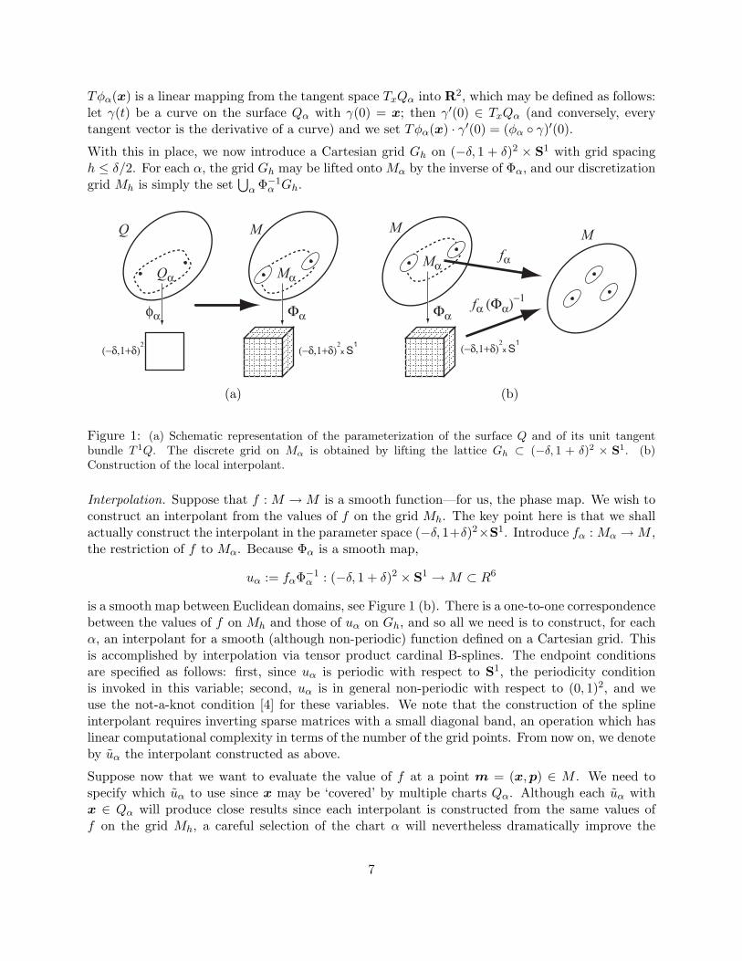
Tφα(x) is a linear mapping from the tangent space TxQα into R2, which may be defined as follows:let γ(t) be a curve on the surface Qα with γ(0) = x; then γ′(0) ∈ TxQα (and conversely, everytangent vector is the derivative of a curve) and we set Tφα(x) · γ′(0) = (φα ◦ γ)′(0).

With this in place, we now introduce a Cartesian grid Gh on (−δ, 1 + δ)2 × S1 with grid spacingh ≤ δ/2. For each α, the grid Gh may be lifted onto Mα by the inverse of Φα, and our discretizationgrid Mh is simply the set

⋃α Φ−1

α Gh.

φα

Qα Mα

Φα

(−δ,1+δ)2

(−δ,1+δ)2x S

1

Q M

Mα

Φα

(−δ,1+δ)2x S

1

M Mfα

fα (Φα)−1

(a) (b)

Figure 1: (a) Schematic representation of the parameterization of the surface Q and of its unit tangentbundle T 1Q. The discrete grid on Mα is obtained by lifting the lattice Gh ⊂ (−δ, 1 + δ)2 × S1. (b)Construction of the local interpolant.

Interpolation. Suppose that f : M →M is a smooth function—for us, the phase map. We wish toconstruct an interpolant from the values of f on the grid Mh. The key point here is that we shallactually construct the interpolant in the parameter space (−δ, 1+δ)2×S1. Introduce fα : Mα →M ,the restriction of f to Mα. Because Φα is a smooth map,

uα := fαΦ−1α : (−δ, 1 + δ)2 × S1 →M ⊂ R6

is a smooth map between Euclidean domains, see Figure 1 (b). There is a one-to-one correspondencebetween the values of f on Mh and those of uα on Gh, and so all we need is to construct, for eachα, an interpolant for a smooth (although non-periodic) function defined on a Cartesian grid. Thisis accomplished by interpolation via tensor product cardinal B-splines. The endpoint conditionsare specified as follows: first, since uα is periodic with respect to S1, the periodicity conditionis invoked in this variable; second, uα is in general non-periodic with respect to (0, 1)2, and weuse the not-a-knot condition [4] for these variables. We note that the construction of the splineinterpolant requires inverting sparse matrices with a small diagonal band, an operation which haslinear computational complexity in terms of the number of the grid points. From now on, we denoteby uα the interpolant constructed as above.

Suppose now that we want to evaluate the value of f at a point m = (x,p) ∈ M . We need tospecify which uα to use since x may be ‘covered’ by multiple charts Qα. Although each uα withx ∈ Qα will produce close results since each interpolant is constructed from the same values off on the grid Mh, a careful selection of the chart α will nevertheless dramatically improve the

7

accuracy. Our selection is guided by the following important observation: when the not-a-knotcondition is used, the interpolation error at points which are at least two gridpoints away fromthe boundary is considerably lower than that at points which are closer to the boundary. This iswhere our assumption becomes handy. Since Q =

⋃α φ

−1α ([0, 1]2) and h ≤ δ/2, we are guaranteed

that for any x ∈ Q, one can choose α(x) such that φα(x)(x) is at least ‘two grid points away’from the boundary. The value of f(x) is then approximated in an obvious fashion, namely, byuα(x)(Φα(x)(x,p)).

ODE integration rule. We work with the 4th order Runge-Kutta method [6] as a local integrationrule. Now, even though any integral curve of (2.1) remains on the surface Q the numerical solutionwill surely deviate from the surface because of the integration error. In order to ensure that theapproximate phase map gt(·) maps M = T 1Q to itself, we impose an extra projection step whichsnaps a point (x,p) ∈ R6 close to M back onto M . In a first step, we perform a Newton-typeiteration

x← x− F (x)|∇F (x)|2

∇F (x)

until |F (x)| ≤ ε, where ε is some prescribed accuracy parameter. Since (x,p) is always close to M ,it usually takes only 3 to 4 iterations even when ε is as small as 10−9. In a second step, we thenproject p onto the plane orthogonal to ∇F (x) (and apply renormalization to keep a unit-lengthvector). This projection step is also invoked during the interpolation wherever the interpolantdeviates from the invariant manifold M .

2.3 Numerical results

This section presents several numerical results. The proposed method is implemented in Matlaband all the computational results reported here were obtained on a desktop computer with a 2.6GHzCPU and 1GB of memory.

We use Algorithm 2 (the modified version of the phase flow method) to construct the geodesic flow.In every example, we set T0 = 1/8 and τ is chosen to be 2−10. To estimate the numerical error, weproceed as follows: we select N points {mi} randomly from M ; the “exact” solutions gT0(mi) arecomputed with Matlab’s adaptive ODE solver with a prescribed error equal to 10−9; the numerical

error is estimated by√∑N

i=1 |gT0(mi)− gT0(mi)|2/N . In all these examples, N = 200.

Example 1. The surface Q is an ellipsoid given by

x2

a2+y2

b2+z2

c2= 1

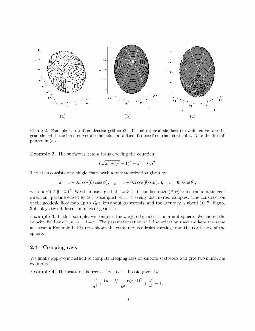
with a = 1.2 and b = c = 0.8. The atlas consists of six charts, each one corresponding to oneof the six principal axes: ±x, ±y and ±z. For every chart, the parameter domain (−δ, 1 + δ) isdiscretized with a Cartesian grid of size 16 × 16, see Figure 2(a) for a plot of the discretizationgrid on Q. We discretize S1, which parameterizes the unit tangent directions, with 64 equispacedpoints. Constructing gT0 takes about 100 seconds and the error is less than 10−6. We then use gT0

to rapidly compute the geodesics starting from a single point, see Figures 2(b) and (c). The blackcurves are solutions at time T = kT0 for integer values of k. The black curves are resolved with1024 samples each.

8

(a) (b) (c)

Figure 2: Example 1. (a) discretization grid on Q. (b) and (c) geodesic flow; the white curves are thegeodesics while the black curves are the points at a fixed distance from the initial point. Note the fish-tailpattern in (c).

Example 2. The surface is here a torus obeying the equation:

(√x2 + y2 − 1)2 + z2 = 0.52.

The atlas consists of a single chart with a parameterization given by

x = 1 + 0.5 cos(θ) cos(ψ), y = 1 + 0.5 cos(θ) sin(ψ), z = 0.5 sin(θ),

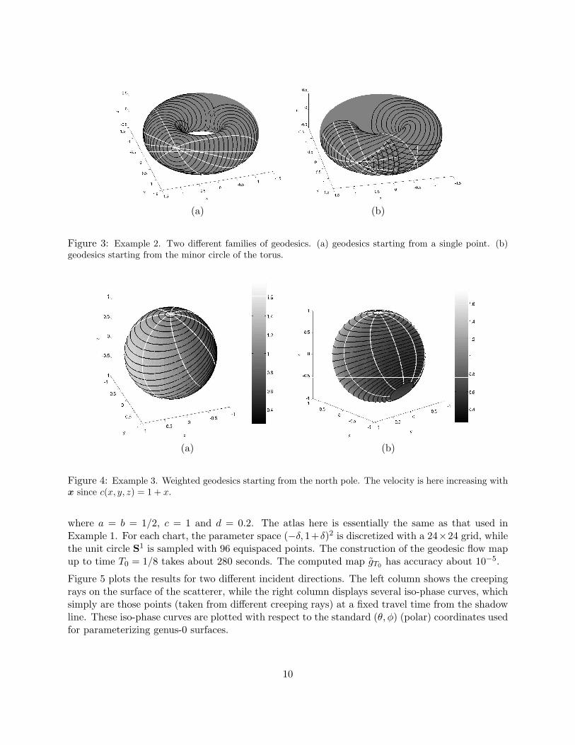
with (θ, ψ) ∈ [0, 2π)2. We then use a grid of size 32× 64 to discretize (θ, ψ) while the unit tangentdirection (parameterized by S1) is sampled with 64 evenly distributed samples. The constructionof the geodesic flow map up to T0 takes about 30 seconds, and the accuracy is about 10−6. Figure3 displays two different families of geodesics.

Example 3. In this example, we compute the weighted geodesics on a unit sphere. We choose thevelocity field as c(x, y, z) = 1 + x. The parameterization and discretization used are here the sameas those in Example 1. Figure 4 shows the computed geodesics starting from the north pole of thesphere.

2.4 Creeping rays

We finally apply our method to compute creeping rays on smooth scatterers and give two numericalexamples.

Example 4. The scatterer is here a “twisted” ellipsoid given by

x2

a2+

(y − d/c · cos(πz))2

b2+z2

c2= 1,

9

(a) (b)

Figure 3: Example 2. Two different families of geodesics. (a) geodesics starting from a single point. (b)geodesics starting from the minor circle of the torus.

(a) (b)

Figure 4: Example 3. Weighted geodesics starting from the north pole. The velocity is here increasing withx since c(x, y, z) = 1 + x.

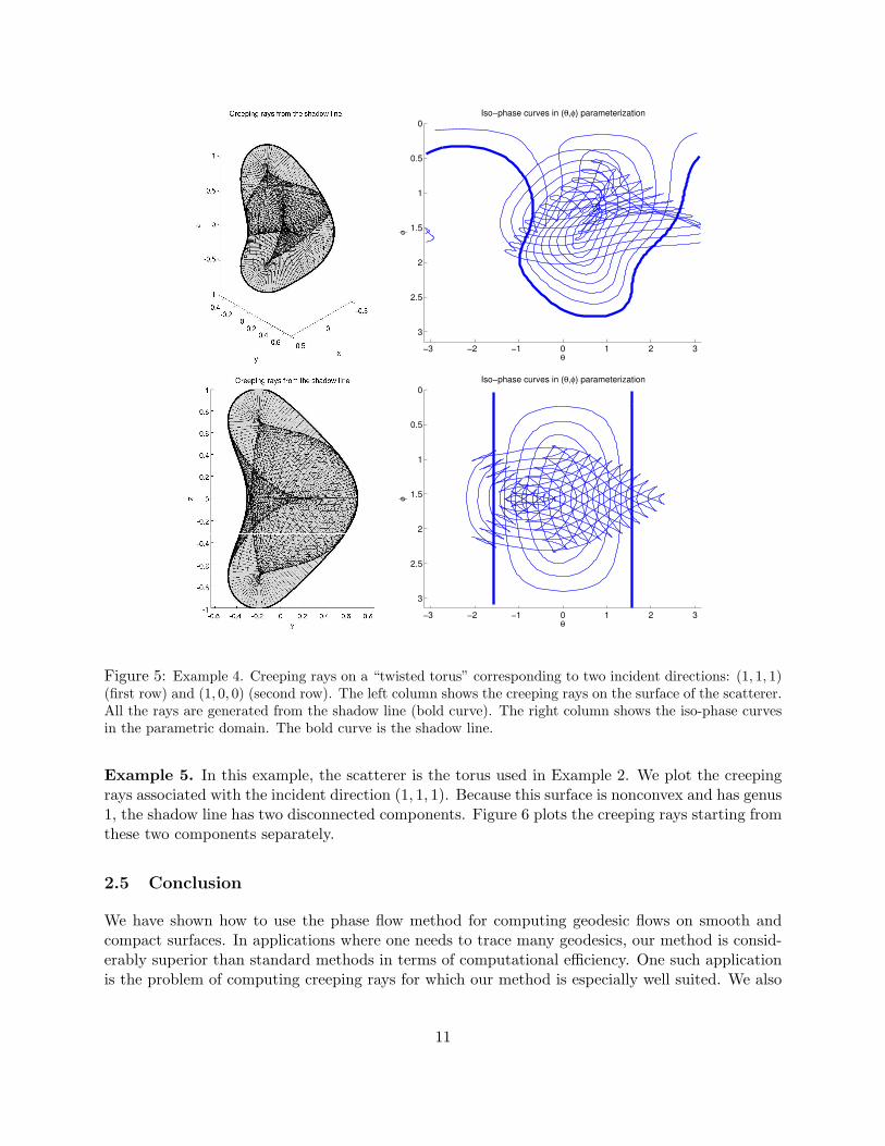
where a = b = 1/2, c = 1 and d = 0.2. The atlas here is essentially the same as that used inExample 1. For each chart, the parameter space (−δ, 1+δ)2 is discretized with a 24×24 grid, whilethe unit circle S1 is sampled with 96 equispaced points. The construction of the geodesic flow mapup to time T0 = 1/8 takes about 280 seconds. The computed map gT0 has accuracy about 10−5.

Figure 5 plots the results for two different incident directions. The left column shows the creepingrays on the surface of the scatterer, while the right column displays several iso-phase curves, whichsimply are those points (taken from different creeping rays) at a fixed travel time from the shadowline. These iso-phase curves are plotted with respect to the standard (θ, φ) (polar) coordinates usedfor parameterizing genus-0 surfaces.

10

−3 −2 −1 0 1 2 3

0

0.5

1

1.5

2

2.5

3

θ

φ

Iso−phase curves in (θ,φ) parameterization

−3 −2 −1 0 1 2 3

0

0.5

1

1.5

2

2.5

3

θ

φ

Iso−phase curves in (θ,φ) parameterization

Figure 5: Example 4. Creeping rays on a “twisted torus” corresponding to two incident directions: (1, 1, 1)(first row) and (1, 0, 0) (second row). The left column shows the creeping rays on the surface of the scatterer.All the rays are generated from the shadow line (bold curve). The right column shows the iso-phase curvesin the parametric domain. The bold curve is the shadow line.

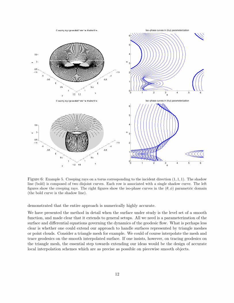
Example 5. In this example, the scatterer is the torus used in Example 2. We plot the creepingrays associated with the incident direction (1, 1, 1). Because this surface is nonconvex and has genus1, the shadow line has two disconnected components. Figure 6 plots the creeping rays starting fromthese two components separately.

2.5 Conclusion

We have shown how to use the phase flow method for computing geodesic flows on smooth andcompact surfaces. In applications where one needs to trace many geodesics, our method is consid-erably superior than standard methods in terms of computational efficiency. One such applicationis the problem of computing creeping rays for which our method is especially well suited. We also

11

0 1 2 3 4 5 60

1

2

3

4

5

6

θ

φ

Iso−phase curves in (θ,φ) parameterization

0 1 2 3 4 5 60

1

2

3

4

5

6

θ

φ

Iso−phase curves in (θ,φ) parameterization

Figure 6: Example 5. Creeping rays on a torus corresponding to the incident direction (1, 1, 1). The shadowline (bold) is composed of two disjoint curves. Each row is associated with a single shadow curve. The leftfigures show the creeping rays. The right figures show the iso-phase curves in the (θ, φ) parametric domain(the bold curve is the shadow line).

demonstrated that the entire approach is numerically highly accurate.

We have presented the method in detail when the surface under study is the level set of a smoothfunction, and made clear that it extends to general setups. All we need is a parameterization of thesurface and differential equations governing the dynamics of the geodesic flow. What is perhaps lessclear is whether one could extend our approach to handle surfaces represented by triangle meshesor point clouds. Consider a triangle mesh for example. We could of course interpolate the mesh andtrace geodesics on the smooth interpolated surface. If one insists, however, on tracing geodesics onthe triangle mesh, the essential step towards extending our ideas would be the design of accuratelocal interpolation schemes which are as precise as possible on piecewise smooth objects.

12

References

[1] V. I. Arnold. Mathematical methods of classical mechanics. Springer-Verlag, New York, 1978. Translatedfrom the Russian by K. Vogtmann and A. Weinstein, Graduate Texts in Mathematics, 60.

[2] M. Born and E. Wolf. Principles of Optics. Cambridge University Press, seventh edition, 1999.

[3] J. Chen and Y. Han. Shortest paths on a polyhedron. I. Computing shortest paths. Internat. J. Comput.Geom. Appl., 6(2):127–144, 1996.

[4] C. de Boor. A practical guide to splines, volume 27 of Applied Mathematical Sciences. Springer-Verlag,New York, revised edition, 2001.

[5] S. Fomel and J. A. Sethian. Fast-phase space computation of multiple arrivals. Proc. Natl. Acad. Sci.USA, 99(11):7329–7334 (electronic), 2002.

[6] A. Iserles. A first course in the numerical analysis of differential equations. Cambridge Texts in AppliedMathematics. Cambridge University Press, Cambridge, 1996.

[7] J. B. Keller and R. M. Lewis. Asymptotic methods for partial differential equations: the reduced waveequation and Maxwell’s equations. In Surveys in applied mathematics, Vol. 1, volume 1 of Surveys Appl.Math., pages 1–82. Plenum, New York, 1995.

[8] R. Kimmel and J. A. Sethian. Computing geodesic paths on manifolds. Proc. Natl. Acad. Sci. USA,95(15):8431–8435 (electronic), 1998.

[9] J. E. Marsden and T. S. Ratiu. Introduction to mechanics and symmetry, volume 17 of Texts in AppliedMathematics. Springer-Verlag, New York, 1994. A basic exposition of classical mechanical systems.

[10] F. Memoli and G. Sapiro. Fast computation of weighted distance functions and geodesics on implicithyper-surfaces. J. Comput. Phys., 173(2):730–764, 2001.

[11] J. S. B. Mitchell, D. M. Mount, and C. H. Papadimitriou. The discrete geodesic problem. SIAM J.Comput., 16(4):647–668, 1987.

[12] M. Motamed and O. Runborg. A fast phase space method for computing creeping rays. Submitted,2005.

[13] J. A. Sethian. A fast marching level set method for monotonically advancing fronts. Proc. Nat. Acad.Sci. U.S.A., 93(4):1591–1595, 1996.

[14] V. Surazhsky, T. Surazhsky, D. Kirsanov, S. J. Gortler, and H. Hoppe. Fast exact and approximategeodesics on meshes. ACM Trans. Graph., 24(3):553–560, 2005.

[15] L. Ying and E. J. Candes. The phase flow method. Technical report, California Institute of Technology,2005. Submitted.

13