Length and Circumference Assessment of Body Parts – The

49th International Conference on Environmental Systems ICES-2019-170 7-11 July 2019, Boston, Massachusetts

Copyright © 2019 Jan P. Weber, Institute of Astronautics, Boltzmannstraße 15, 85748 Garching b. München

Length and Circumference Assessment of Body Parts – The Creation of Easy-To-Use Predictions Formulas

Jan P. Weber1 Technische Universität München, 85748 Garching b. München, Germany

The Virtual Habitat project (V-HAB) at the Technical University of Munich (TUM) aims to develop a dynamic simulation environment for life support systems (LSS). Within V-HAB a dynamic human model interacts with the LSS by providing relevant metabolic inputs and outputs based on internal, environmental and operational factors. The human model is separated into five sub-models (called layers) representing metabolism, respiration, thermoregulation, water balance and digestion. The Wissler Thermal Model was converted in 2015/16 from Fortran to C#, introducing a more modularized structure and standalone graphical user interface (GUI). While previous effort was conducted in order to make the model in its current accepted version available in V-HAB, present work is focusing on the rework of the passive system. As part of this rework an extensive assessment of human body measurements and their dependency on a low number of influencing parameters was performed using the body measurements of 3982 humans (1774 men and 2208 women) in order to create a set of easy-to-use predictive formulas for the calculation of length and circumference measurements of various body parts.

Nomenclature AAC = Axillary Arm Circumference Age = Age of the subject ARL = Acromion-Radiale Length BCF = Biceps Circumference, Flexed BMI = Body Mass Index BUC = Buttock Circumference CAC = Calf Circumference CAH = Calf Height CEH = Cervicale Height CHC = Chest Circumference CHCBB = Chest Circumference Below Breast CRH = Crotch Height dkg = deci-kilogram EC = Elbow Circumference EHS = Eye Height, Sitting F = Female FAC = Forearm Circumference FHL = Forearm-Hand Length GUI = Graphic User Interface HC = Head Circumference ICRP = International Commission on

Radiological Protection KC = Knee Circumference

1 External Researcher, M.Sc., Institute of Astronautics, Boltzmannstraße 15, Building 6 /2nd Floor.

KHM = Knee Height, Midpatella LSS = Life Support System LTC = Lower Thigh Circumference M = Male NC = Neck Circumference NC = New Convection Calculation NG = New Geometry NP = New Properties RSL = Radiale-Stylion Length SH = Sitting Height SSH = Suprasternale Height Stature = Height of the subject TC = Thigh Circumference TRH = Tenth Rib height TUM = Technical University of Munich V-HAB = Virtual Habitat VO2MAX = maximal oxygen consumption WCN = Waist Circumference (Natural

Indentation) WCO = Waist Circumference (Omphalion) Weight = Weight of the subject WH = Wrist Height WRC = Wrist Circumference

International Conference on Environmental Systems

2

I. Introduction ITHIN the past five decades the Wissler Thermal Model became one of the most sophisticated and well accepted human thermal models today, especially gaining strong acceptance in the field of aerospace

engineering. Within this time frame it underwent several iterations1–5 with changes both in structure of the human build-up (especially fidelity) and the underlying simulation algorithms. Today the Wissler Thermal Model consists of 21 right-circular cylinders representing the human body. While the Wissler Thermal Model is accepted by many entities, the author found that the model is lacking in documentation (e.g. code commenting), shows physical properties which are not in alignment with data reported in literature and most obviously lacks in the prediction of the human build-up (both externally and internally)6,7. While previous research by the author7 was intended as a topical review of the general findings, this year paper is intended to describe the findings in more detail and show the approach taken by the author to improve the Wissler Thermal Model.

A. The 2009 Wissler Human Thermal Model The newest iteration of the Wissler Human Thermal Model was published by E.H. Wissler in 20095. The model

consists of 21 right-circular cylinders representing the human. Two elements represent the head and neck, three the torso, while each arm and leg are separated into four cylinders as shown in Figure 1. Each cylinder is sub-divided into 15 nodal layers of tissue and up-to a further six layers for clothing representation. Each nodal layer is itself sub-divided into 12 angular nodes to account for angular changes within each layer / element. Each of the up-to 5061 nodes contains (depending whether it is a tissue or clothing node) data about the local physical and physiological properties such as density, thermal conductivity, specific heat, temperature, blood perfusion rate and metabolic rate. As described in an earlier publication8 the Wissler Thermal Model incorporates many features such as distributed energy production (depending on the local metabolic rate assigned to each node and the activity performed during the simulation), axial heat transfer between the elements via blood, and radial heat transfer using an alternating direction implicit numerical method to calculate the heat transfer via conduction in the elements5.

As mentioned in a previous paper7 the development of the 2009 model E.H. Wissler was strongly influenced by the work of Fiala et al.9,10 as Prof. Wissler states himself. This influence was also observed by the author in the code, both by the formulas / approaches chosen to model certain physiological behaviors and when comparing the physical properties used within the Wissler Thermal Model to the published values by Fiala et al.

Figure 1. Graphical Representation of the Wissler Human Thermal Model

B. The external Structure of the 2009 Wissler Thermal Model During the translation of the Wissler Human Thermal Model from Fortran to C# (described in an earlier paper8)

the author discovered that the physical, external measurements were not simulated correctly within the model. It was found that a standard male, as described by the ICRP (International Commission on Radiological Protection) (73 [kg];

W


3

1760 [mm])11, is calculated about 115 [mm] smaller, resulting in a compressed simulated subject, as the Wissler Human Thermal Model was still predicting the weight of the simulated human correctly. This lead to the conclusion that the external build-up would need to be reworked. But since this would lead to possible changes or distortions in the (local) simulation of organs and/or tissues such as muscle, bone or fat it was decided that the entire build-up, both externally and internally would need to be reassessed, analyzed and subsequently reworked.

C. Approach As stated within Ref. 7, the author realized that the Wissler Human Thermal Model, as received from E.H. Wissler

in 2013, is lacking in documentation and code commenting and that a revision and optimization of the current model would be needed. Therefore the author decided to perform an in depth assessment, analysis and subsequent rework of the passive model, starting with the rework of the external build-up (body measurements), internal build-up (tissue representation at each node and therefore assessment of organ size/ weight and tissue distribution within the body and within each element of the Wissler Thermal Model), which will be published in a dedicated paper alongside this one, and the assessment of physical properties of the main tissues within the human body (paper under preparation).

II. Materials, Methods and Assessment The anthropometry of the human body i.e. the knowledge of the measurements of the human body becomes very

important for the construction of the human body in a human thermal simulation program. High variance in body height, weight, age and gender – to name only a few factors influencing human body measurements, causes difficulties to accurately predict body measurements of various body parts depending on the person to be simulated.

There are many standards available referencing and reporting values for human body measurements such as the NASA-STD-3000, EN ISO 7250 or DIN 33402. The problem with these standards is that body measurements for all people vary a lot. Additionally, other factors such as the ethnical background may influence the ability to adapt measurements gained from a standard for a certain limited part of the population to another one. For example, the NASA-STD-3000 explicitly states:

Data are provided for the 5th percentile Asian Japanese and 95th percentile White or Black American Male projected to the year 2000. This does not necessarily define the 5th and 95th percentile of the user population. The data in this document are meant only to provide information on the size ranges of people of the world. The Japanese female represents some of the smaller people of the world and the American male some of the larger.12

Values are normally available in data tables or as average values accompanied by the 5th, 50th and 95th percentile showing statistic mean and extrema for a studied population.

Newer standards such as the NASA-STD-300113 refer to that “each program shall identify or develop an anthropometry, biomechanics, aerobic capacity, and strength data set for the crewmember population to be accommodated”, thereby showing the importance for program tailored data sets and information to gain specifically for the target population – as intended by the author of this paper.

The current rework of the Wissler Thermal Model done by the author is intended to simulate astronauts within the

V-HAB project’s simulation environment, being of various ethnicities and mainly flying in their fourth to sixth decade (only six astronauts were 60 or older during their last flight: Pavel V. Vinogradov, Gregory H. Olsen, Paolo Nespoli, Dennis A. Tito, Franklin S. Musgrave and John H. Glenn – Michael W. Mevill is not counted in as he only conducted suborbital flights with SpaceShipOne) but being selected at the age of about 30 to 35 it was decided that a large data collection would be needed. Therefore, the author searched for a dataset covering medium to well-trained humans (as e.g. astronauts intend to be well trained) of mainly Caucasian and/or mixed American origin. The dataset used for the following analysis is the “1988 Anthropometric Survey of U.S. Army Personnel: Methods and Summary Statistics” conducted by Gordon et al.14.

In the late 1980’s Gordon et al. conducted a wide data assessment of anthropometric measurements for the U.S. Army to gather data to improve and guide the design and sizing of equipment, clothing and other hardware used. A total of 25811 subjects were screened for the study and of these 8997 were selected for full measurement. This included the recording of information such as age, race, ethnic identity, rank, grade and army occupation and 132 body measurements, which were seen as the most useful for meeting the needs of clothing, work space, human analog design and more. Of these 8997 subjects (5506 male and 3491 female) a subsample of 1774 men and 2208 women was selected to represent the proportions of age and racial/ethnic found in June 1988 in the U.S. Army as shown in Table 1 and Table 2.


4

Table 1. Demographic Distribution of Measured Males Age White Black Hispanic Asian/Pacific

Island American Indian / Alaskan Native

Other

≤ 20 12.63% 3.78% 0.56% 0.23% 0.11% 0.28%

21-24 17.93% 6.93% 0.90% 0.34% 0.11% 0.51%

25-30 15.39% 7.67% 1.07% 0.39% 0.11% 0.62%

≥ 31 20.12% 7.44% 1.30% 0.62% 0.34% 0.62%

Table 2. Demographic Distribution of Measured Females Age White Black Hispanic Asian/Pacific

Island American Indian / Alaskan Native

Other

≤ 20 9.47% 5.89% 0.45% 0.23% 0.14% 0.27%

21-24 15.44% 12.50% 0.72% 0.36% 0.23% 0.59%

25-30 15.04% 14.99% 0.82% 0.41% 0.14% 0.59%

≥ 31 11.68% 8.38% 0.63% 0.45% 0.14% 0.45%

The sampling carried out by Gordon et al. was done carefully as “sampling is the single most critical element of

an anthropometric survey”14. As each measurement decision decided prior to measurement will have effects on all later calculated statistical measures such as mean value or standard deviation.

The survey of Gordon et al. was carried out with four objectives in mind14: 1) Accurately and comprehensively represent the range of body sizes of current U.S. Army Personnel; 2) Accurately and comprehensively represent the body size of the U.S. Army in the year 2000 and beyond; 3) Contain adequate numbers in various demographic subgroups to answer basic research questions about the

nature of human variability by race and age; 4) Contain adequate numbers in specific occupational subgroups (e.g. armor and aviation) so that end-items of

personal protective equipment can be designed around the anthropometry of individuals in those specific groups where meaningful differences between groups are found to exist.

The datasets shown in Table 1 and Table 2 were created based on the fact, that earlier studies15–17 had shown that both age and race are extremely important in influencing body size and shape. Therefore, a stratified random sampling plan was created to select subjects representing the intended U.S. Army target population.

Different to the intention of Gordon et al. the author’s intention is to gain knowledge and eventually create

regression formulas to predict the body element measurements by a few influencing input values for the simulation of astronauts within the Wissler Thermal Model. Since neither the age nor the racial/ethnical proportions in the study of Gordon et al. resemble the ones for astronauts, it was decided to create a subset of the data of Gordon et al. This was also driven by the fact, that some subjects either showed very high or low Body Mass Index (BM) values. It was decided that only data measured from subjects with a BMI of 18.5 to 25.0 – which is considered as medically normal – will be studied for the analysis and creation of regression formulas. 811 men and 1613 women met this requirement. The male subject’s age ranged from 17 to 48 with an average age of 25.7 years, the weight ranged from 47.6 to 89.3 [kg] with an average weight of 70.52 [kg] and the stature ranged from 1497 [mm] to 2042 [mm] with an average stature of 1755.1 [mm]. The female subject’s age ranged from 18 to 50 with an average age of 25.5 years, the weight ranged from 41.3 [kg] to 87.4 [kg] with an average weight of 59.34 [kg] and the stature ranged from 1428 [mm] to 1870 [mm] with an average stature of 1630.1 [mm].

A total of 12 length measurements and 16 circumference measurements (cf. Table 3) out of the 132 measurements for each subject collected by Gordon et al. were identified to benefit calculation of regression formulas for the prediction of body elements within the Wissler Thermal Model. The in Table 3 listed 28 body measurements out of the available 132 were chosen in a way that they benefit the estimation of various major body sections the best to estimate the volume of each body section as close as possible with regards to the simplified cylindrical build-up of the Wissler Thermal Model’s modelling setup. The landmarks at or between which these measurements are taken can be looked up within the survey of Gordon et al.14 and will therefore not be explained here.


5

Table 3. Values Analyzed in Regression Analysis Length Measurement Circumference Measurement

Acromion-Radiale Length (ARL) Axillary Arm Circumference (AAC) Calf Height (CAH) Biceps Circumference, Flexed (BCF)

Cervicale Height (CEH) Buttock Circumference (BUC) Crotch Height (CRH) Calf Circumference (CAC)

Eye Height, Sitting (EHS) Chest Circumference (CHC) Forearm-Hand Length (FHL) Chest Circumference Below Breast (CHCBB)

Knee Height, Midpatella (KHM) Elbow Circumference (EC) Radiale-Stylion Length (RSL) Forearm Circumference (FAC)

Sitting Height (SH) Head Circumference (HC) Suprasternale Height (SSH) Knee Circumference (KC)

Tenth Rib Height (TRH) Lower Thigh Circumference (LTC) Wrist Height (WH) Neck Circumference (NC)

Thigh Circumference (TC) Waist Circumference (Natural Indentation) (WCN) Waist Circumference (Omphalion) (WCO) Wrist Circumference (WRC)

In order to analyze if a regression analysis for the datasets for the 28 in Table 3 listed measurements can be

performed (e.g. using the t-test) the normal distribution was assessed using the Kolmogorov-Smirnov nonparametric test, comparing the gained data from the subsets created by the author from the data of Gordon et al. to a reference probability distribution in order to gain data about the goodness-of-fit. It was decided to use the Kolmogorov-Smirnov test as other tests like the Shapiro-Wilk test do not work well in samples with many identical values (which happened to occur for specific measurements in the present datasets) or like the Anderson-Darling test showing more sensitivity to deviations in tails, hence assigning more weight to the tails than the Kolmogorov-Smirnov test does18,19. The results of the goodness-of-fit analysis is shown in Table 4 and Table 5. The critical value for the Kolmogorov-Smirnov test was calculated using the estimation formula shown in equation 1 for a n > 3519. The critical values in Table 4 and Table 5 are calculated with a statistical significance α = 0.05. For male subjects (811 in total) the critical value using equation 1 is 0.0477 [-], while for female subjects (1613 in total) the critical value is 0.0338 [-]. For the conduction of the Kolmogorov-Smirnov test and the subsequent regression analysis the author used Microsoft Excel and the included statistics package and relied on the statistical explanations provided by Bohm and Zech18 and Sachs and Hedderich19. The term “possibly” was added to Table 4 and Table 5 columns titled “Normal Distribution Assessment” as the Kolmogorov-Smirnov test’s p-value, respectively the test statistic (KS-Value) quantifies and indicates that a sample does (to an extent that is unlikely to arise merely by chance) or does not diverge from a normal distribution.

𝑑" =$%&'()*

√,- (1)

Of all 56 assessments performed, 8 were found to be possibly not normal distributed according to the Kolmogorov-

Smirnov test performed, as described above. For men this is the FAC, for women this is the RSL, BCF, CHCBB, EC, HC, WCO and WRC. For these eight values the Q-Q-Plots are shown in Figure 2 through Figure 9, to show graphically the difference between both the assumed, theoretical and real distribution. Within each Q-Q-Plot shown below the vertical axis shows the real, observed values, while the horizontal axis shows the theoretical values of the standard distribution.


6

Table 4. Goodness-Of-Fit Analysis with Kolmogorov-Smirnov Test for 811 Male subjects for 28 body measurements

Measurement Range Average Standard Div.

KS-Value

Normal Distribution Assessment

Acromion-Radiale Length (ARL) 271-415 339.45 17.13 0.0403 Possibly Normal Distributed

Calf Height (CAH) 271-442 352.96 24.01 0.0448 Possibly Normal Distributed

Cervicale Height (CEH) 1267-1776 1516.36 64.09 0.0241 Possibly Normal Distributed

Crotch Height (CRH) 675-1067 841.95 46.60 0.0320 Possibly Normal Distributed

Eye Height, Sitting (EHS) 673-902 790.54 35.22 0.0290 Possibly Normal Distributed

Forearm-Hand Length (FHL) 386-578 482.06 22.95 0.0437 Possibly Normal Distributed

Knee Height, Midpatella (KHM) 406-620 504.25 27.88 0.0380 Possibly Normal Distributed

Radiale-Stylion Length (RSL) 212-325 268.97 15.53 0.0399 Possibly Normal Distributed

Sitting Height (SH) 808-1032 912.03 36.63 0.0185 Possibly Normal Distributed

Suprasternale Height (SSH) 1188-1686 1434.94 60.18 0.0234 Possibly Normal Distributed

Tenth Rib Height (TRH) 905-1353 1118.91 52.56 0.0248 Possibly Normal Distributed

Wrist Height (WH) 702-995 844.10 42.63 0.0230 Possibly Normal Distributed

Axillary Arm Circumference (AAC) 245-366 314.98 17.82 0.0292 Possibly Normal Distributed

Biceps Circumference, Flexed (BCF) 260-376 319.85 19.30 0.0360 Possibly Normal Distributed

Buttock Circumference (BUC) 805-1053 937.06 40.01 0.0293 Possibly Normal Distributed

Calf Circumference (CAC) 304-424 361.58 19.44 0.0204 Possibly Normal Distributed

Chest Circumference (CHC) 775-1081 942.21 44.44 0.0225 Possibly Normal Distributed Chest Circumference Below Breast

(CHCBB) 723-1015 880.16 42.27 0.0229 Possibly Normal Distributed

Elbow Circumference (EC) 219-302 267.72 11.53 0.0344 Possibly Normal Distributed

Forearm Circumference (FAC) 244-335 292.62 14.36 0.0507 Possibly Not Normal Distributed

Head Circumference (HC) 514-615 562.61 13.99 0.0304 Possibly Normal Distributed

Knee Circumference (KC) 317-433 372.01 16.66 0.0406 Possibly Normal Distributed

Lower Thigh Circumference (LTC) 309-446 372.72 19.32 0.0274 Possibly Normal Distributed

Neck Circumference (NC) 325-409 368.03 14.55 0.0324 Possibly Normal Distributed

Thigh Circumference (TC) 458-640 558.14 31.64 0.0388 Possibly Normal Distributed Waist Circumference (Natural

Indentation) (WCN) 647-932 785.11 44.26 0.0185 Possibly Normal Distributed

Waist Circumference (Omphalion) (WCO) 654-1004 799.14 52.65 0.0325 Possibly Normal Distributed

Wrist Circumference (WRC) 145-192 170.56 7.25 0.0390 Possibly Normal Distributed


7

Table 5. Goodness-Of-Fit Analysis with Kolmogorov-Smirnov Test for 1613 Female subjects for 28 body measurements

Measurement Range Average Standard Div.

KS-Value

Normal Distribution Assessment

Acromion-Radiale Length (ARL) 262-370 311.61 16.62 0.0322 Possibly Normal Distributed

Calf Height (CAH) 249-413 315.95 23.86 0.0299 Possibly Normal Distributed

Cervicale Height (CEH) 1212-1643 1408.08 59.49 0.0209 Possibly Normal Distributed

Crotch Height (CRH) 638-948 773.18 44.24 0.0192 Possibly Normal Distributed

Eye Height, Sitting (EHS) 640-854 738.55 33.41 0.0234 Possibly Normal Distributed

Forearm-Hand Length (FHL) 373-546 442.62 23.47 0.0228 Possibly Normal Distributed

Knee Height, Midpatella (KHM) 378-584 459.20 26.01 0.0250 Possibly Normal Distributed

Radiale-Stylion Length (RSL) 201-312 243.53 15.44 0.0370 Possibly Not Normal Distributed

Sitting Height (SH) 748-971 851.74 35.16 0.0233 Possibly Normal Distributed

Suprasternale Height (SSH) 1151-1538 1330.41 56.25 0.0232 Possibly Normal Distributed

Tenth Rib Height (TRH) 883-1243 1045.09 48.83 0.0206 Possibly Normal Distributed

Wrist Height (WH) 673-939 789.57 38.82 0.0229 Possibly Normal Distributed

Axillary Arm Circumference (AAC) 225-346 283.51 17.68 0.0282 Possibly Normal Distributed

Biceps Circumference, Flexed (BCF) 227-332 274.07 16.66 0.0346 Possibly Not Normal Distributed

Buttock Circumference (BUC) 812-1130 948.74 47.08 0.0171 Possibly Normal Distributed

Calf Circumference (CAC) 291-415 346.73 19.28 0.0336 Possibly Normal Distributed

Chest Circumference (CHC) 745-1083 887.14 46.89 0.0254 Possibly Normal Distributed Chest Circumference Below Breast

(CHCBB) 641-909 754.24 38.39 0.0473 Possibly Not Normal Distributed

Elbow Circumference (EC) 202-272 234.58 10.57 0.0346 Possibly Not Normal Distributed

Forearm Circumference (FAC) 211-295 249.88 12.28 0.0307 Possibly Normal Distributed

Head Circumference (HC) 500-603 544.84 14.08 0.0422 Possibly Not Normal Distributed

Knee Circumference (KC) 303-433 359.07 18.62 0.0248 Possibly Normal Distributed

Lower Thigh Circumference (LTC) 304-455 369.90 21.54 0.0169 Possibly Normal Distributed

Neck Circumference (NC) 272-357 312.09 12.70 0.0325 Possibly Normal Distributed

Thigh Circumference (TC) 464-713 566.02 33.35 0.0146 Possibly Normal Distributed Waist Circumference (Natural

Indentation) (WCN) 568-883 703.88 43.10 0.0319 Possibly Normal Distributed

Waist Circumference (Omphalion) (WCO) 627-1009 764.34 59.57 0.0449 Possibly Not Normal

Distributed

Wrist Circumference (WRC) 129-174 149.99 6.31 0.0693 Possibly Not Normal Distributed


8

Figure 2. Q-Q-Plot – Forearm Circumference,

Flexed (FAC) – Men

Figure 3. Q-Q-Plot – Radiale-Stylion Length

(RSL) – Women

Figure 4. Q-Q-Plot – Biceps Circumference,

Flexed (BCF) – Women

Figure 5. Q-Q-Plot – Chest Circumference Below

Breast (CHCBB) – Women

Figure 6. Q-Q-Plot – Elbow Circumference (EC)

– Women

Figure 7. Q-Q-Plot – Head Circumference (HC) –

Women

-4

-3

-2

-1

0

1

2

3

4

-4 -3 -2 -1 0 1 2 3 4

-4

-3

-2

-1

0

1

2

3

4

5

-4 -3 -2 -1 0 1 2 3 4

-4

-3

-2

-1

0

1

2

3

4

-4 -3 -2 -1 0 1 2 3 4

-4

-3

-2

-1

0

1

2

3

4

5

-4 -3 -2 -1 0 1 2 3 4

-4

-3

-2

-1

0

1

2

3

4

-4 -3 -2 -1 0 1 2 3 4

-4

-3

-2

-1

0

1

2

3

4

5

-4 -3 -2 -1 0 1 2 3 4


9

Figure 8. Q-Q-Plot – Waist Circumference

Omphalion (WCO) – Women

Figure 9. Q-Q-Plot – Wrist Circumference

(WRC) – Women

The Q-Q-Plots indicate that all datasets identified by the Kolmogorov-Smirnov test are positive/right-skewed, in which the mass of the distribution is concentrated left of the normal distribution, with the plot for the Waist Circumference at the Omphalion showing the strongest skewness.

Comparing the Q-Q-Plots for the eight by the Kolmogorov-Smirnov test identified datasets as not normal distributed we can assess, that all, but the WCO and WRC for women distribute more or less normal. The reason for this is that the Kolmogorov-Smirnov test, similar to other tests mentioned above, tends to produce small significance levels or large KS-Values and thereby more often rejects the null-hypothesis with a higher sample number being analyzed. The reason why WRC is assessed to be not normal distributed is based on the results of the Kolmogorov-Smirnov test and the visual analysis using the Q-Q-Plot in Figure 9, in which most of the values are on the left side of the diagonal line. Though being only slightly left of this, it indicates a constant positive /right-skewed dataset.

One of the requirements of multiple linear regression is the normal distribution of the residual. As shown above

all but two datasets fulfill this requirement. While – in general – it is possible to perform a transformation of the independent and / or dependent variables in order to gain normality, this itself can cause problems. On the other hand, more robust regression analysis methods than the classical normal linear regression could be used. But for most cases the multiple linear regression is sufficient robust against the violation of the normal distribution assumption. Therefore, it was decided that a multiple linear regression analysis using t-test could be performed on all datasets, especially giving the large size of the datasets (811 for men 1613 for women).

Since the author’s intention is to create Easy-To-Use prediction formulas for the estimation of body elements. It

was decided that all input parameters and therefore all parameters analyzed as independent variables in the regression analysis need to be easy to measure or at best always known, as it seemed impractical to first measure certain body lengths or circumferences at specific landmarks without a good knowledge where and what to measure and subsequently calculate the remaining body measurements by ratios.

As a first approach the author decided to use three independent values, height/stature [mm], weight [dkg] and age [years] as easy to measure inputs to regression formulas. The decision to use these three values is based on the findings of Gordon et al.14 mentioning that “stature and weight are excellent descriptors of overall body size” and further studies15–17 – as mentioned before – which had shown that both age and race are extremely important in influencing body size and shape. While the first three are easy to measure, specific analysis for race was put aside, as only sufficient data for Caucasian and African American subject could be obtained. Therefore, the author decided that a multiple linear regression analysis using height, weight and age for the mix-ethnic subset of the dataset of Gordon et al. would be sufficient for a first approach.

Linear regression was used because of ease of use and analyses were all performed to obtain the best possible R2 results. Whenever the multiple linear regression analysis was indicating that only one of the three independent variables (height, weight or age) has a significant influence on the dependent variable, a simple linear regression analysis was performed (regression analysis involving age of the subject was only performed in form of multiple linear regression analysis and never alone). Table 6 and Table 7 show the R2 and significance levels of each formula

-4

-3

-2

-1

0

1

2

3

4

5

-4 -3 -2 -1 0 1 2 3 4

-4

-3

-2

-1

0

1

2

3

4

5

-4 -3 -2 -1 0 1 2 3 4


10

generating the best possible R2 and the formula itself for both male and female subjects. The significance level was left empty in the two tables when the independent variable had no influence in the prediction.

It can be noted, that height predictions using simple single or multiple linear regression are more likely to achieve good correlation than circumference predictions as most height and length measurements more or less strongly correlate with the overall stature of the subjects. In contrast to that all circumference measurements in both male and female subjects with the exception of head and knee circumference (HC and NC) in male use multiple linear regression formulas either including all three independent variables or at least height and weight. While in general good and sometimes very good correlations were achieved with values of 0.45 and above, the overall worst correlation were achieved for the head circumference with R2 = 0.16 in male, respectively R2 = 0.15 in female and the neck circumference with R2 = 0.40 in male, respectively R2 = 0.37 in female.

Table 6. Multiple Linear Regression Analysis for 28 Measurements in Male Formula R2 pheight pweight page

𝐴𝑅𝐿1 = 0.1998 ∙ 𝑆𝑡𝑎𝑡𝑢𝑟𝑒 − 11.267 0.63 < 0.001 - - 𝐶𝐴𝐻10.2603 ∙ 𝑆𝑡𝑎𝑡𝑢𝑟𝑒 − 0.2314 ∙ 𝐴𝑔𝑒 − 97.918 0.55 < 0.001 - 0.010

𝐶𝐸𝐻1 = 0.9318 ∙ 𝑆𝑡𝑎𝑡𝑢𝑟𝑒 + 0.2522 ∙ 𝐴𝑔𝑒 − 125.513 0.97 < 0.001 - < 0.001 𝐶𝑅𝐻1 = 0.6408 ∙ 𝑆𝑡𝑎𝑡𝑢𝑟𝑒 − 0.068 ∙ 𝑊𝑒𝑖𝑔ℎ𝑡– 0.3429 ∙ 𝐴𝑔𝑒 − 226.189 0.74 < 0.001 < 0.001 0.009

𝐸𝐻𝑆1 = 0.3777 ∙ 𝑆𝑡𝑎𝑡𝑢𝑟𝑒 + 0.4734 ∙ 𝐴𝑔𝑒 + 115.488 0.53 < 0.001 - < 0.001 𝐹𝐻𝐿1 = 0.2374 ∙ 𝑆𝑡𝑎𝑡𝑢𝑟𝑒 + 0.0245 ∙ 𝑊𝑒𝑖𝑔ℎ𝑡 + 48.206 0.58 < 0.001 0.037 -

𝐾𝐻𝑀1 = 0.3476 ∙ 𝑆𝑡𝑎𝑡𝑢𝑟𝑒 − 105.730 0.72 < 0.001 - - 𝑅𝑆𝐿1 = 0.1616 ∙ 𝑆𝑡𝑎𝑡𝑢𝑟𝑒 − 14.597 0.50 < 0.001 - -

𝑆𝐻1 = 0.3975 ∙ 𝑆𝑡𝑎𝑡𝑢𝑟𝑒 + 0.3642 ∙ 𝐴𝑔𝑒 + 204.991 0.54 < 0.001 - < 0.001 𝑆𝑆𝐻1 = 0.8702 ∙ 𝑆𝑡𝑎𝑡𝑢𝑟𝑒 − 92.260 0.96 < 0.001 - - 𝑇𝑅𝐻1 = 0.7201 ∙ 𝑆𝑡𝑎𝑡𝑢𝑟𝑒 − 144.930 0.86 < 0.001 - - 𝑊𝐻1 = 0.5486 ∙ 𝑆𝑡𝑎𝑡𝑢𝑟𝑒 − 118.705 0.76 < 0.001 - -

𝐴𝐴𝐶1 =−0.1419 ∙ 𝑆𝑡𝑎𝑡𝑢𝑟𝑒 + 0.2752 ∙ 𝑊𝑒𝑖𝑔ℎ𝑡– 0.2609 ∙ 𝐴𝑔𝑒 + 376.660 0.56 < 0.001 < 0.001 < 0.001 𝐵𝐶𝐹1 =−0.1422 ∙ 𝑆𝑡𝑎𝑡𝑢𝑟𝑒 + 0.2680 ∙ 𝑊𝑒𝑖𝑔ℎ𝑡– 0.4294 ∙ 𝐴𝑔𝑒 + 391.513 0.45 < 0.001 < 0.001 < 0.001

𝐵𝑈𝐶1 =−0.1276 ∙ 𝑆𝑡𝑎𝑡𝑢𝑟𝑒 + 0.5976 ∙ 𝑊𝑒𝑖𝑔ℎ𝑡 + 739.460 0.78 < 0.001 < 0.001 - 𝐶𝐴𝐶1 =−0.0915 ∙ 𝑆𝑡𝑎𝑡𝑢𝑟𝑒 + 0.2596 ∙ 𝑊𝑒𝑖𝑔ℎ𝑡– 0.2042 ∙ 𝐴𝑔𝑒 + 344.300 0.51 < 0.001 < 0.001 0.007 𝐶𝐻𝐶1 =−0.2029 ∙ 𝑆𝑡𝑎𝑡𝑢𝑟𝑒 + 0.6255 ∙ 𝑊𝑒𝑖𝑔ℎ𝑡 + 0.6543 ∙ 𝐴𝑔𝑒 + 840.373 0.60 < 0.001 < 0.001 < 0.001 𝐶𝐻𝐶𝐵𝐵1 = −0.1786 ∙ 𝑆𝑡𝑎𝑡𝑢𝑟𝑒 + 0.5705 ∙ 𝑊𝑒𝑖𝑔ℎ𝑡 + 1.0537 ∙ 𝐴𝑔𝑒 + 764.223 0.58 < 0.001 < 0.001 < 0.001

𝐸𝐶1 =−0.0156 ∙ 𝑆𝑡𝑎𝑡𝑢𝑟𝑒 + 0.1398 ∙ 𝑊𝑒𝑖𝑔ℎ𝑡 + 196.518 0.60 0.008 < 0.001 - 𝐹𝐴𝐶1 =−0.0503 ∙ 𝑆𝑡𝑎𝑡𝑢𝑟𝑒 + 0.1616 ∙ 𝑊𝑒𝑖𝑔ℎ𝑡– 0.1978 ∙ 𝐴𝑔𝑒 + 271.968 0.38 < 0.001 < 0.001 0.002

𝐻𝐶1 = 0.0802 ∙ 𝑊𝑒𝑖𝑔ℎ𝑡 + 506.028 0.16 - < 0.001 - 𝐾𝐶1 = 0.1889 ∙ 𝑊𝑒𝑖𝑔ℎ𝑡 + 238.763 0.62 - < 0.001 -

𝐿𝑇𝐶1 =−0.0872 ∙ 𝑆𝑡𝑎𝑡𝑢𝑟𝑒 + 0.2751 ∙ 𝑊𝑒𝑖𝑔ℎ𝑡 + 331.819 0.61 < 0.001 < 0.001 - 𝑁𝐶1 =−0.0475 ∙ 𝑆𝑡𝑎𝑡𝑢𝑟𝑒 + 0.1652 ∙ 𝑊𝑒𝑖𝑔ℎ𝑡– 0.1483 ∙ 𝐴𝑔𝑒 + 338.705 0.40 < 0.001 < 0.001 0.017 𝑇𝐶1 =−0.2548 ∙ 𝑆𝑡𝑎𝑡𝑢𝑟𝑒 + 0.5482 ∙ 𝑊𝑒𝑖𝑔ℎ𝑡 − 0.5480 ∙ 𝐴𝑔𝑒 + 632.714 0.74 < 0.001 < 0.001 < 0.001 𝑊𝐶𝑁1 = −0.2323 ∙ 𝑆𝑡𝑎𝑡𝑢𝑟𝑒 + 0.6219 ∙ 𝑊𝑒𝑖𝑔ℎ𝑡 + 1.9886 ∙ 𝐴𝑔𝑒 + 703.138 0.64 < 0.001 < 0.001 < 0.001 𝑊𝐶𝑂1 = −0.2058 ∙ 𝑆𝑡𝑎𝑡𝑢𝑟𝑒 + 0.6756 ∙ 𝑊𝑒𝑖𝑔ℎ𝑡 + 2.2624 ∙ 𝐴𝑔𝑒 + 625.813 0.59 < 0.001 < 0.001 < 0.001

𝑊𝑅𝐶1 = 0.0148 ∙ 𝑆𝑡𝑎𝑡𝑢𝑟𝑒 + 0.0588 ∙ 𝑊𝑒𝑖𝑔ℎ𝑡 + 103.107 0.46 < 0.001 < 0.001 -

III. The Rework of the Wissler Human Thermal Model The development of a human thermal model is often a compromise between the fidelity of the simulation model

and the representation of the real person. Most human models such as the one of E. H. Wissler use cylinders to simulate human body parts. On the one hand, simulation of cylinders makes a model both simpler in construction and to understand but on the other hand can cause difficulties in the overall predictive capabilities. Especially certain body regions such as the hands, feet and the upper part of the cranium/head cause difficulties as they do not resemble cylinders. Additionally, these elements show high surface to volume ratios which are difficult to account for in models using solely cylindrical elements, where the cylinder lateral surface is the only area of heat dissipation to the outside. In order to generate formulas for the 21 body elements for length and radius measurements within the Wissler Human Thermal Model the in section II. derived and in Table 6 and Table 7 shown regression formulas were used. The rework within this section focused, as previously mentioned, on subjects with a BMI considered as normal (18.5 to 25). Furthermore, the rework of the cylinders, due to the amount of work considered with it and the subsequently needed rework of the internal body element buildup was – for the moment – performed for male subjects only. A paper for


11

female subjects is currently under preparation. Within the 811 male subjects in the subset of the survey (fulfilling the BMI requirement of 18.5 to 25), all but 23 were younger than 40 years. Therefore, the primary age range in which these formulas are applicable is 20 to 40 years of age. Additionally, most subjects weighted between 54 and 85 [kg] and were between 1.58 and 1.88 [m] tall. Therefore, all formulas for male subjects gained from the regression analysis in section II. and within this section are mainly applicable within these input parameter ranges.

It shall be noted, that due to simplicity reasons, as done by E.H. Wissler previously, there was no difference made between right and left extremities measurements (real humans tend to have a dominant side which shows slightly larger body part volumes).

Table 7. Multiple Linear Regression Analysis for 28 Measurements in Female

Formula R2 pheight pweight page

𝐴𝑅𝐿W = 0.2033 ∙ 𝑆𝑡𝑎𝑡𝑢𝑟𝑒 − 19.872 0.61 < 0.001 - - 𝐶𝐴𝐻W = 0.2321 ∙ 𝑆𝑡𝑎𝑡𝑢𝑟𝑒 + 0.0265 ∙ 𝑊𝑒𝑖𝑔ℎ𝑡 − 0.2565 ∙ 𝐴𝑔𝑒 − 71.623 0.45 < 0.001 0.010 0.002

𝐶𝐸𝐻W = 0.9099 ∙ 𝑆𝑡𝑎𝑡𝑢𝑟𝑒 + 0.0132 ∙ 𝑊𝑒𝑖𝑔ℎ𝑡 − 82.984 0.97 < 0.001 0.027 - 𝐶𝑅𝐻W = 0.6209 ∙ 𝑆𝑡𝑎𝑡𝑢𝑟𝑒 − 0.0511 ∙ 𝑊𝑒𝑖𝑔ℎ𝑡– 0.5591 ∙ 𝐴𝑔𝑒 − 194.355 0.72 < 0.001 < 0.001 < 0.001

𝐸𝐻𝑆W = 0.3923 ∙ 𝑆𝑡𝑎𝑡𝑢𝑟𝑒 + 0.3375 ∙ 𝐴𝑔𝑒 + 90.489 0.56 < 0.001 - < 0.001 𝐹𝐻𝐿W = 0.2470 ∙ 𝑆𝑡𝑎𝑡𝑢𝑟𝑒 + 0.0234 ∙ 𝑊𝑒𝑖𝑔ℎ𝑡 + 26.027 0.51 < 0.001 0.014 -

𝐾𝐻𝑀W = 0.3374 ∙ 𝑆𝑡𝑎𝑡𝑢𝑟𝑒 − 90.785 0.68 < 0.001 - - 𝑅𝑆𝐿W = 0.1605 ∙ 𝑆𝑡𝑎𝑡𝑢𝑟𝑒 − 18.053 0.44 < 0.001 - - 𝑆𝐻W = 0.4157 ∙ 𝑆𝑡𝑎𝑡𝑢𝑟𝑒 + 174.075 0.57 < 0.001 - -

𝑆𝑆𝐻W = 0.8454 ∙ 𝑆𝑡𝑎𝑡𝑢𝑟𝑒 + 0.0315 ∙ 𝑊𝑒𝑖𝑔ℎ𝑡 − 66.323 0.97 < 0.001 < 0.001 - 𝑇𝑅𝐻W = 0.7149 ∙ 𝑆𝑡𝑎𝑡𝑢𝑟𝑒 − 0.2839 ∙ 𝐴𝑔𝑒 − 113.081 0.87 < 0.001 - < 0.001

𝑊𝐻W = 0.5188 ∙ 𝑆𝑡𝑎𝑡𝑢𝑟𝑒 − 56.071 0.73 < 0.001 - - 𝐴𝐴𝐶W =−0.1423 ∙ 𝑆𝑡𝑎𝑡𝑢𝑟𝑒 + 0.3027 ∙ 𝑊𝑒𝑖𝑔ℎ𝑡– 0.1967 ∙ 𝐴𝑔𝑒 + 340.878 0.59 < 0.001 < 0.001 < 0.001

𝐵𝐶𝐹W =−0.1276 ∙ 𝑆𝑡𝑎𝑡𝑢𝑟𝑒 + 0.2727 ∙ 𝑊𝑒𝑖𝑔ℎ𝑡 + 320.221 0.55 < 0.001 < 0.001 - 𝐵𝑈𝐶W =−0.1797 ∙ 𝑆𝑡𝑎𝑡𝑢𝑟𝑒 + 0.7695 ∙ 𝑊𝑒𝑖𝑔ℎ𝑡 + 0.7951 ∙ 𝐴𝑔𝑒 + 764.794 0.74 < 0.001 < 0.001 < 0.001 𝐶𝐴𝐶W =−0.0675 ∙ 𝑆𝑡𝑎𝑡𝑢𝑟𝑒 + 0.2601 ∙ 𝑊𝑒𝑖𝑔ℎ𝑡– 0.3850 ∙ 𝐴𝑔𝑒 + 312.215 0.47 < 0.001 < 0.001 < 0.001

𝐶𝐻𝐶W =−0.2664 ∙ 𝑆𝑡𝑎𝑡𝑢𝑟𝑒 + 0.7181 ∙ 𝑊𝑒𝑖𝑔ℎ𝑡 + 895.366 0.53 < 0.001 < 0.001 - 𝐶𝐻𝐶𝐵𝐵W =−0.1423 ∙ 𝑆𝑡𝑎𝑡𝑢𝑟𝑒 + 0.5224 ∙ 𝑊𝑒𝑖𝑔ℎ𝑡 + 676.141 0.47 < 0.001 < 0.001 -

𝐸𝐶W =−0.0093 ∙ 𝑆𝑡𝑎𝑡𝑢𝑟𝑒 + 0.1414 ∙ 𝑊𝑒𝑖𝑔ℎ𝑡– 0.0923 ∙ 𝐴𝑔𝑒 + 168.238 0.61 0.012 < 0.001 0.003 𝐹𝐴𝐶W =−0.0332 ∙ 𝑆𝑡𝑎𝑡𝑢𝑟𝑒 + 0.1572 ∙ 𝑊𝑒𝑖𝑔ℎ𝑡– 0.2137 ∙ 𝐴𝑔𝑒 + 216.235 0.45 < 0.001 < 0.001 < 0.001

𝐻𝐶W = 0.0239 ∙ 𝑆𝑡𝑎𝑡𝑢𝑟𝑒 + 0.0712 ∙ 𝑊𝑒𝑖𝑔ℎ𝑡 + 463.587 0.15 0.001 < 0.001 - 𝐾𝐶W =−0.0351 ∙ 𝑆𝑡𝑎𝑡𝑢𝑟𝑒 + 0.2607 ∙ 𝑊𝑒𝑖𝑔ℎ𝑡 − 0.1088 ∙ 𝐴𝑔𝑒 + 264.467 0.60 < 0.001 < 0.001 0.046

𝐿𝑇𝐶W =−0.1017 ∙ 𝑆𝑡𝑎𝑡𝑢𝑟𝑒 + 0.3364 ∙ 𝑊𝑒𝑖𝑔ℎ𝑡 + 336.100 0.59 < 0.001 < 0.001 - 𝑁𝐶W =−0.0162 ∙ 𝑆𝑡𝑎𝑡𝑢𝑟𝑒 + 0.1375 ∙ 𝑊𝑒𝑖𝑔ℎ𝑡– 0.2627 ∙ 𝐴𝑔𝑒 + 263.588 0.37 0.004 < 0.001 < 0.001

𝑇𝐶W =−0.2233 ∙ 𝑆𝑡𝑎𝑡𝑢𝑟𝑒 + 0.6077 ∙ 𝑊𝑒𝑖𝑔ℎ𝑡 + 569.313 0.75 < 0.001 < 0.001 - 𝑊𝐶𝑁W = −0.2704 ∙ 𝑆𝑡𝑎𝑡𝑢𝑟𝑒 + 0.6814 ∙ 𝑊𝑒𝑖𝑔ℎ𝑡 + 0.9131 ∙ 𝐴𝑔𝑒 + 717.017 0.57 < 0.001 < 0.001 < 0.001 𝑊𝐶𝑂W = −0.3211 ∙ 𝑆𝑡𝑎𝑡𝑢𝑟𝑒 + 0.8149 ∙ 𝑊𝑒𝑖𝑔ℎ𝑡 + 1.2448 ∙ 𝐴𝑔𝑒 + 772.427 0.43 < 0.001 < 0.001 < 0.001 𝑊𝑅𝐶W = 0.0232 ∙ 𝑆𝑡𝑎𝑡𝑢𝑟𝑒 + 0.0503 ∙ 𝑊𝑒𝑖𝑔ℎ𝑡 − 0.0674 ∙ 𝐴𝑔𝑒 + 84.086 0.46 < 0.001 < 0.001 0.002

For each of the 21 body elements suitable measurements from the list provided in Table 3 were selected for the

estimation of the element height and radius. The elements were described by a) what kind of main tissues types and organs are located within each element and b) from which to which point in height each element is extending. This was primarily done, because in the Wissler Human Thermal Model no real information is provided from which to which point each body element is extending and why the implemented measurements were chosen. The definition of the exact location of the body elements with respect to real human body parts shall provide more precise information about the included tissue types and tissue locations within each element.

A. Cranium (Element 1) The cranium mainly reaches from the top of the simulated body down to the virtual line connecting the lower part

of the eye cavity with the most outreaching point on the back of the head/skull. Only parts of the cerebellum and the brainstem reach lower than this virtual line. It was therefore decided that the height of the cranium in male can be best described by the difference between EHS and SH as shown in equation 2.


12

𝐶𝑟𝑎𝑛𝑖𝑢𝑚Z[\]Z^ = 𝑆𝐻 − 𝐸𝐻𝑆 = 0.0198 ∙ 𝑆𝑡𝑎𝑡𝑢𝑟𝑒 − 0.1092 ∙ 𝐴𝑔𝑒 + 89.503 (2) The radius for the cranium is a bit more difficult to be assessed than the height since the cranium is not cylindrical

shaped but instead has the shape of stretched half sphere. As shown in section II. a regression formula for the head circumference was found showing poor correlation (R2 = 0.16) for male subjects, but other formulas published such as the ones of Bale et al.20 do not show better agreement.

Since the head is not ideally cylindrical shaped the radius needs to be adjusted since the thermal model can only simulate cylindrical elements with uniform radius and uniform height. Therefore, the author anticipated that the radius for simulation is only 85% of the radius gained from the HC formula.

𝐶𝑟𝑎𝑛𝑖𝑢𝑚_à\bc = 0.85 ∙ de

,∙f= g.ghi,∙j[\]Z^klmg.n,l

,∙f (3)

B. Lower Head and Neck (Element 2) The lower head and neck element is the second topmost part in the simulated body. In comparison to the cranium

the lower head and neck height and radius estimations are much more difficult. This problem is caused by the basic build-up of the Wissler Thermal Model using only two elements to simulate the head and neck and three elements simulating the torso. Wissler does not explicitly state where these elements start and end in height. To overcome this problem the author decided that element 2 would extend in height from the virtual line described in section III.A. down to the middle between the CH and the SSH in order to cover the lower head and neck down to the cervicale landmark and additionally sharing 50% of the height of the transition region from neck to shoulders (to be precise sharing 50% of the height between the cervicale landmark and the suprasternale landmark with the torso).

The height can subsequently be estimated as shown in equation 4:

𝐿𝑜𝑤𝑒𝑟𝐻𝑒𝑎𝑑𝑁𝑒𝑐𝑘Z[\]Z^ = 𝑆𝑡𝑎𝑡𝑢𝑟𝑒 − 𝐶𝑟𝑎𝑛𝑖𝑢𝑚Z[\]Z^ −(ttdkeud)

,= (4)

= 0.0792 ∙ 𝑆𝑡𝑎𝑡𝑢𝑟𝑒 − 0.0169 ∙ 𝐴𝑔𝑒 + 19.384 As with the cranium, the average radius of the lower head and neck element is a bit more difficult to be assessed.

It was estimated that the lower head is contributing two third to the average radius. This is unfortunately a very rough, purely intuitive estimation based on the author’s estimation of height ratios between lower head and neck which is based on various anatomical drawings of the lower head and neck section (e.g. the ones of Eycleshymer and Schoemaker21). Additionally, a multiplication factor of 90% is assumed – similar to the one applied to the cranium radius estimation – to overcome the not ideal shape of the head especially in the head-neck transition are.

𝐿𝑜𝑤𝑒𝑟𝐻𝑒𝑎𝑑𝑁𝑒𝑐𝑘_à\bc = 0.9 ∙ wek,∙de

,∙f∙m= (5)

=−0.0143 ∙ 𝑆𝑡𝑎𝑡𝑢𝑟𝑒 + 0.0977 ∙ 𝑊𝑒𝑖𝑔ℎ𝑡 − 0.0445 ∙ 𝐴𝑔𝑒 + 405.228

2 ∙ 𝜋

C. Upper Thorax (Element 3) The upper thorax is the third element of the simulated body. Following the build-up of the previous two elements

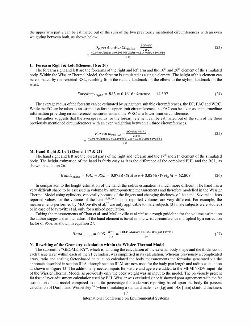
described above and the information extracted from the Wissler Thermal Model, it was assessed, that the thorax includes everything down to the lower end of the lung lobes. The author therefore assessed, that the thorax would reach from the lower point of element 2 (virtual point between the height of the cervicale landmark and the suprasternale landmark) down to the height of the virtual line 28 shown in Figure 10 as the lowest point of the lung. To estimate the lowest point of the lung (height of the diaphragm), it was assessed (cf. section II.D.) that the liver’s lower right lobe closes in height with the rib cage and therefore with the TRH. The height of the lower thorax (cf. section II.D.) can then be used to estimate the height of the upper thorax as shown in equation 6.

𝑈𝑝𝑝𝑒𝑟𝑇ℎ𝑜𝑟𝑎𝑥Z[\]Z^ =

ttdkeud,

− 𝐿𝑜𝑤𝑒𝑟𝑇ℎ𝑜𝑟𝑎𝑥Z[\]Z^ − 𝑇𝑅𝐻 = (6) = 0.1276 ∙ 𝑆𝑡𝑎𝑡𝑢𝑟𝑒 − 0.0158 ∙ 𝑊𝑒𝑖𝑔ℎ𝑡 + 0.0464 ∙ 𝐴𝑔𝑒 + 4.8975


13

The radius of this element can be best estimated in male subjects using the CHC if multiplied by a correction factor intuitively chosen by the author based on estimations using cross section pictures and volume analysis of the upper thorax22, indicating that the upper torso has its maximum circumference at about the height of the chest, while parts of the upper torso below and above this point retract (seen from the side of the male subject) to the coronal plane, while a frontal view on the subject is rather indicating a rectangular shape of the torso (cf. Figure 11 and Figure 12) down to some centimeters below the chest. This led to the estimation that a correction factor of 95% of the calculate CHC would be suitable for male subjects, as shown in equation 7.

Figure 10. Reconstruction picture showing the

thoracic and abdominal viscera and reference levels of various organs21

Figure 11. Side view of the upper body14

Figure 12. Front view of the upper body14

𝑈𝑝𝑝𝑒𝑟𝑇ℎ𝑜𝑟𝑎𝑥_à\bc = 0.95 ∙ ede

,∙f= (7)

= {g.n|,i∙t^`^b_[kg.}|l,∙j[\]Z^kg.h,nh∙~][k�|i.m}l,∙f

D. Lower Thorax (Element 4) The lower thorax is the fourth element of the simulated body. As mentioned, shorty in section III.C. the separation

line between upper thorax and lower thorax was chosen based on the estimated height of the diaphragm (located right below the lungs) at the height of the virtual line 28 shown in Figure 10. This virtual line is therefore serving as the upper limit of the lower thorax element while the lower limit is given by the lowest point of the right lobe of the liver. The author anticipated that the liver’s right lower lobe closes in height with the right rib cage and therefore with the TRH. This anticipation is based on various sources21,23–27, and it shall be noted to avoid confusion, that the lowest point of the right lobe of the liver reported by Eycleshymer and Schoemaker and therefore shown in Figure 10 is considerably lower than the average low point reported, being only 1.0 to 1.5 centimeter above the iliac crest. Other sources such as Cunningham and Merkel23,24 state that the lowest right lobe of the liver reaches a bit below the lower edge of the chest (costal margin), while Corning, Joessel and von Langer and Toldt25–27 report that the lowest right lobe of the liver corresponds in height with the costal margin.

The height of element 4 can therefore be estimated by using Figure 10. Assuming that the virtual lines drawing in Figure 10 are more or less equally spaced in height, 21.5 line spaces between the suprasternal notch (inferior point of the sternum / top of the breastbone) and the crotch and five line spaces between the virtual line 28 (upper limit of the lower thorax) and line 33 (closing line of the costal margin) resulting in the height estimation for the lower thorax shown in equation 8.


14

𝐿𝑜𝑤𝑒𝑟𝑇ℎ𝑜𝑟𝑎𝑥Z[\]Z^ =

ttd{e�d,n.}

∙ 5 = (8) = 0.0533 ∙ 𝑆𝑡𝑎𝑡𝑢𝑟𝑒 + 0.0158 ∙ 𝑊𝑒𝑖𝑔ℎ𝑡 + 0.0797 ∙ 𝐴𝑔𝑒 + 31.146

The radius of the lower thorax can be estimated using the CHCBB as the upper circumference of the lower thorax,

while the lower circumference is well estimated by the WCN. The CHCBB is measured at the height of the inferior juncture of the lowest breast with the rib cage, being at about the height of the virtual line 28 and therefore perfectly suitable for the estimation of the upper circumference of the lower thorax element. The WCN is measured at the height of maximum natural indentation and therefore actually about 2.5 centimeters too low compared to the TRH but due to a missing value for the circumference at the TRH the best estimation for this circumference from the dataset of Gordon et al.

𝐿𝑜𝑤𝑒𝑟𝑇ℎ𝑜𝑟𝑎𝑥_à\bc =

ede��kjew,∙f∙,

= (9)

= {g.,g}}∙t^`^b_[kg.}|h,∙j[\]Z^kn.},n,∙~][k�mm.hin,∙f

E. Abdomen & Pelvis (Element 5) The abdomen and pelvis is the fifth element of the simulated body and due to the estimation of the previous four

elements fairly easy to be estimated in height, as it is reaching from the lower end of the lower thorax from the TRH down to CRH. Because of this assumption of extension of the abdomen and pelvis element and due to the fact that within the Wissler Thermal Model only cylinders can be simulated parts of the flaps need to be included into the abdomen and pelvis element with the legs being “cut off” at the height of the crotch (between virtual lines 43 and 44 in Figure 10).

𝐴𝑏𝑑𝑜𝑚𝑑𝑒𝑛𝑃𝑒𝑙𝑣𝑖𝑠Z[\]Z^ =

��d{e�d,

= (10) = 0.0793 ∙ 𝑆𝑡𝑎𝑡𝑢𝑟𝑒 + 0.0680 ∙ 𝑊𝑒𝑖𝑔ℎ𝑡 + 0.3429 ∙ 𝐴𝑔𝑒 + 81.259

The radius of this element can be estimated using three suitable circumference measurements from the dataset of

Gordon et al., the WCN, WCO and BUC. As previously discussed (cf. section II.D.), the WCN can be taken as the lower limit circumference for the lower thorax and therefore as the upper limit circumference of the abdomen and pelvis element. The WCO serves can serve as an intermediate information providing circumference measurements at the height of the navel, while the BUC serves as an information providing circumference at the height or the maximum protrusion.

For male an average radius out of the sum of the three previously mentioned circumferences is suggested with an even weighting between all three circumferences.

𝐴𝑏𝑑𝑜𝑚𝑒𝑛𝑃𝑒𝑙𝑣𝑖𝑠_à\bc =

jewkje�k��e,∙f∙m

= (11)

= {g.niih∙t^`^b_[kg.hmn�∙j[\]Z^kn.ln�g∙~][khi|.l�g,∙f

F. Upper Thigh Right & Left (Element 6 & 10) The upper thigh right and left are the sixth and tenth element of the simulated body. Within the Wissler Thermal

Model, the upper leg is split into two elements, the upper and lower thigh (cf. section III.G.). For simplicity reasons and because there is no distinct separation within the thigh possible (both in male and female) the height of the overall thigh is equally distributed between upper and lower thigh. The height of the overall thigh can be estimated as the difference between the CRH and the KHM resulting in the estimation formula showing in equation 12 for the upper thigh:

𝑈𝑝𝑝𝑒𝑟𝑇ℎ𝑖𝑔ℎZ[\]Z^ =

e�d{�w1,

= (12) = 0.1466 ∙ 𝑆𝑡𝑎𝑡𝑢𝑟𝑒 − 0.0340 ∙ 𝑊𝑒𝑖𝑔ℎ𝑡 − 0.1715 ∙ 𝐴𝑔𝑒 − 60.230

The radius of the upper thighs can be estimated by assuming a uniform circumference over the full height of the

upper thigh equal to the circumference that can be estimated using the TC.


15

𝑈𝑝𝑝𝑒𝑟𝑇ℎ𝑖𝑔ℎ_à\bc =

�e,∙f

= (13)

= {g.,}li∙t^`^b_[kg.}li,∙j[\]Z^{g.}lig∙~][khm,.�nl,∙f

G. Lower Thigh Right & Left (Element 7 & 11) The lower thigh right and left are the lower thighs on the right and left leg and the seventh and eleventh element

of the simulated body. The height of the lower thighs is, as previously mentioned (cf. section III.F.), the same of the upper thigh, since the overall thigh height between CRH and KHM are equally distributed between upper and lower thigh.

𝐿𝑜𝑤𝑒𝑟𝑇ℎ𝑖𝑔ℎZ[\]Z^ =

e�d{�w1,

= (14) = 0.1466 ∙ 𝑆𝑡𝑎𝑡𝑢𝑟𝑒 − 0.0340 ∙ 𝑊𝑒𝑖𝑔ℎ𝑡 − 0.1715 ∙ 𝐴𝑔𝑒 − 60.230

The radius of the lower thighs can be estimated by using three suitable circumferences from the dataset of Gordon

et al., TC, KC and LTC. While the TC can be taken as an predictor for the upper limit circumference in the absence of a better alternative, the LTC can be taken as an intermediate information providing a circumference estimation at the height of the suprapatellar landmark at the top of the knee and the KC as the lower limit circumference.

Due to the irregular, first slightly conic and later between LTC and KC slightly cylindrical/oval shape, of the lower thigh the estimation of an average radius based on the three above mentioned and available circumferences for this body part is difficult. The author suggests that the average radius for the lower thigh element can be estimated out of the sum of the three previously mentioned circumferences with an even weighting between all three circumferences.

𝐿𝑜𝑤𝑒𝑟𝑇ℎ𝑖𝑔ℎ_à\bc =

�ek��ek�e,∙f∙m

= (15)

= {g.nnlg∙t^`^b_[kg.mm�l∙j[\]Z^{g.ni,�∙~][klgn.g||,∙f

H. Calf Right & Left (Element 8 & 12) The calf right and left are the calves on the right and left leg and the eighth and twelfth element of the simulated

body. The height estimation for the calf for the simulation is a bit difficult, since the only reference measurement in height for this section are the KHM and the CAH (height of maximum circumference at the calf). Unfortunately, there is no height of the foot or any height in the lower calf region reported in the available database. Therefore, the author estimated by using images and drawings of the human body by Eycleshymer and Schoemaker21 and Gordon et al.14 and by using the distance between KHM and CAH as a reference for about half the calf height, that the element height of the simulated calf can be best estimated by multiplying the KHM with two-third. It shall be noted that this calculated calf height might not correspond to distances between KHM and ankle since it is an estimation.

𝐶𝑎𝑙𝑓Z[\]Z^ =

,m∙ 𝐾𝐻𝑀 = 0.2317 ∙ 𝑆𝑡𝑎𝑡𝑢𝑟𝑒 − 70.487 (16)

The radius estimation of the calf element is again difficult due the irregular shape formed by the various muscles

within the calf. Because of this fact and the predominant shape giving character of the muscles in the calf for the whole calf the author decided that the best average radius estimation for the calf element in the simulation could be achieved by multiplying the CAC with a correction factor of 80% as shown in equation 17.

𝐶𝑎𝑙𝑓_à\bc = 0.8 ∙ e~e

,∙f= (17)

= {g.g�m,∙t^`^b_[kg.,g��∙j[\]Z^{g.nhml∙~][k,�}.llg,∙f

I. Lower Leg & Foot Right & Left (Element 9 & 13) The lower leg and foot are the lowest parts of the right and left leg and the ninth and 13th element in the simulated

body. The height estimation is fairly easy since the lower leg and foot height is the lower third of the height from ground to KHM as discussed above (cf. section III.H.).


16

𝐿𝑜𝑤𝑒𝑟𝐿𝑒𝑔𝐹𝑜𝑜𝑡Z[\]Z^ =nm∙ 𝐾𝐻𝑀 = 0.1159 ∙ 𝑆𝑡𝑎𝑡𝑢𝑟𝑒 − 35.243 (18)

In comparison to that the average radius estimation for the lower leg parts and foot is much more difficult. Not only because the lower leg and foot first stretches in vertical direction in the lower leg and ankle while then transitioning to stretch in a horizontal direction, being impossible to be modelled like this within the Wissler Thermal Model (and virtually any other human thermal model relying on cylinders as element shape), but also because of the very difficult shape of this element. The lower leg is first more cylindrical while then transitioning to an oval shape in the hind foot region and then to more and more flat getting oval shapes in the mid and forefoot (cross-section wise). The problem with the Wissler Thermal Model is that the cylinder simulated will not have the same thermal behavior as a real lower leg and feet since the overall skin area will be different (this can be compensated with the usage of weighing factors for heat exchange via the different skin surfaces) and the build-up of a cylinder is different to the one of the foot. The best approximation of the average radius of the lower leg and foot is achieved if it is 90% of the estimated radius of the simulated calf element. The gained volumes calculated from LowerLegFootheight (see above) and LowerLegFootradius (see below) show good correspondence with the volumes of the foot reported by McConville et al.22 (when the values reported by McConville et al. are corrected to the weight of the simulated subject / standard male6).

𝐿𝑜𝑤𝑒𝑟𝐿𝑒𝑔𝐹𝑜𝑜𝑡_à\bc = 0.9 ∙ 𝐶𝑎𝑙𝑓_à\bc = 0.72 ∙ e~e

,∙f= (19)

= {g.gh}|∙t^`^b_[kg.nih|∙j[\]Z^{g.nl�g∙~][k,l�.i|h,∙f

J. Upper Arm Part 1 Right & left (Element 14 & 18) The upper arm part 1 right and left are the upper arm parts of the right and left upper arm and the 14th and 18th

element of the simulated body. Within the Wissler Thermal Model the upper arm is split into two elements the upper arm part 1 and the upper arm part 2 (cf. section III.K.). For simplicity reasons and because there is no distinct separation within the upper arm possible the height of the overall upper arm is equally distributed between both parts within the simulation. The height of the overall upper arm is given by the ARL, reaching from the acromion landmark on the shoulder to the radiale landmark on the elbow.

𝑈𝑝𝑝𝑒𝑟𝐴𝑟𝑚𝑃𝑎𝑟𝑡1Z[\]Z^ =

~��,= 0.0999 ∙ 𝑆𝑡𝑎𝑡𝑢𝑟𝑒 − 5.634 (20)

The average radius of the upper arm part 1 can be estimates by using two suitable circumferences, the AAC and

the BCF. While the AAC can be taken as an estimator for the upper limit circumference, the BCF can be taken as a lower limit circumference for the upper part of the upper arm. The author suggests that the average radius for the simulation of the upper arm part 1 can be estimated out of the sum of the two previously mentioned circumferences with an even weighting between both, as shown below.

𝑈𝑝𝑝𝑒𝑟𝐴𝑟𝑚𝑃𝑎𝑟𝑡1_à\bc =~~ek�eW,∙f∙,

= (21)

= {g.nl,n∙t^`^b_[kg.,�nh∙j[\]Z^{g.ml},∙~][kmil.gi�,∙f

K. Upper Arm Part 2 Right & Left (Element 15 & 19) The upper arm part 2 right and left is the lower part of the right and left upper arm and the 15th and 19th element

of the simulated body. The height of the lower part of the upper arm is, as previously mentioned (cf. section III.J.), the same as of the upper part of the upper arm, since the overall ARL is equally distributed between upper and lower part (part 1 and 2).

𝑈𝑝𝑝𝑒𝑟𝐴𝑟𝑚𝑃𝑎𝑟𝑡1Z[\]Z^ =

~��,= 0.0999 ∙ 𝑆𝑡𝑎𝑡𝑢𝑟𝑒 − 5.634 (22)

The average radius of the upper arm part 2 can be estimated by using two suitable circumferences, the BCF and EC. While the BCF can be taken as an estimator for the upper limit circumference, the EC can be taken as a lower limit circumference for the lower part of the upper arm. The author suggests that the average radius for the simulation of


17

the upper arm part 2 can be estimated out of the sum of the two previously mentioned circumferences with an even weighting between both, as shown below.

𝑈𝑝𝑝𝑒𝑟𝐴𝑟𝑚𝑃𝑎𝑟𝑡2_à\bc =�eWkue,∙f∙,

= (23)

= {g.g�i|∙t^`^b_[kg.,gm|∙j[\]Z^{g.,nl�∙~][k,|l.gnh,∙f

L. Forearm Right & Left (Element 16 & 20) The forearm right and left are the forearms of the right and left arm and the 16th and 20th element of the simulated

body. Within the Wissler Thermal Model, the forearm is simulated as a single element. The height of this element can be estimated by the reported RSL, reaching from the radiale landmark on the elbow to the stylion landmark on the wrist.

𝐹𝑜𝑟𝑒𝑎𝑟𝑚Z[\]Z^ = 𝑅𝑆𝐿 = 0.1616 ∙ 𝑆𝑡𝑎𝑡𝑢𝑟𝑒 − 14.597 (24)

The average radius of the forearm can be estimated by using three suitable circumferences, the EC, FAC and WRC. While the EC can be taken as an estimation for the upper limit circumference, the FAC can be taken as an intermediate information providing circumference measurement and the WRC as a lower limit circumference.

The author suggests that the average radius for the forearm element can be estimated out of the sum of the three previously mentioned circumferences with an even weighting between all three circumferences.

𝐹𝑜𝑟𝑒𝑎𝑟𝑚_à\bc =

uekW~ekj�e,∙f∙m

= (25)

= {g.gn�g∙t^`^b_[kg.n,gn∙j[\]Z^{g.gh}|∙~][kn|g.}mn,∙f

M. Hand Right & Left (Element 17 & 21) The hand right and left are the lowest parts of the right and left arm and the 17th and 21st element of the simulated

body. The height estimation of the hand is fairly easy as it is the difference of the combined FHL and the RSL, as shown in equation 26.

𝐻𝑎𝑛𝑑Z[\]Z^ = 𝐹𝐻𝐿 − 𝑅𝑆𝐿 = 0.0758 ∙ 𝑆𝑡𝑎𝑡𝑢𝑟𝑒 + 0.0245 ∙ 𝑊𝑒𝑖𝑔ℎ𝑡 + 62.803 (26) In comparison to the height estimation of the hand, the radius estimation is much more difficult. The hand has a

very difficult shape to be assessed in volume by anthropometric measurements and therefore modelled in the Wissler Thermal Model using cylinders, especially because of the fingers and changing thickness of the hand. Several authors reported values for the volume of the hand22,28,29 but the reported volumes are very different. For example, the measurements performed by McConville et al.22 are only applicable to male subjects (31 male subjects were studied) or in case of Mayrovitz et al. only for a mixed population.

Taking the measurements of Chau et al. and McConville et al.22,28 as a rough guideline for the volume estimation the author suggests that the radius of the hand element is based on the wrist circumference multiplied by a correction factor of 95%, as shown in equation 27.

𝐻𝑎𝑛𝑑_à\bc = 0.95 ∙ j�e

,∙f= g.gnln∙t^`^b_[kg.g}}|∙j[\]Z^k|�.|},

,∙f (27)

N. Rewriting of the Geometry calculation within the Wissler Thermal Model The subroutine “GEOMETRY”, which is handling the calculation of the external body shape and the thickness of

each tissue layer within each of the 21 cylinders, was simplified in its calculation. Whereas previously a complicated array, ratio and scaling factor-based calculation calculated the body measurements the formulas generated via the approach described in section III.A. through section III.M. are now used for the body part length and radius calculation as shown in Figure 13. The additionally needed inputs for stature and age were added to the MEMINSDV input file of the Wissler Thermal Model, as previously only the body weight was an input to the model. The previously present fat tissue layer adjustment calculation used by E.H. Wissler was excluded since it showed poor agreement with the fat estimation of the model compared to the fat percentage the code was reporting based upon the body fat percent calculation of Durnin and Womersley 30 (when simulating a standard male – 73 [kg] and 14.6 [mm] skinfold thickness


18

with the original code provided by E.H. Wissler, the fat weight is estimated to be about 152607 [g] –– while the body weight within the simulation is calculated to be 73.5 [kg] resulting in a fat percentage of 20.76% compared to the estimation of Durnin and Womersley within the model of 23.65%).

The remaining structure of the subroutine was kept as previously used. The only difference is that instead of assuming an average skin thickness of 1.5 [mm] at each body element an array-based calculation containing the thicknesses of dermis and epidermis (Figure 14) is now used, as described in another paper published along this one31.

O. Assessment of the remodeled human Using the data gained from this widespread assessment of body measurements, regression analysis and the

subsequent generation of estimation formulas for the Wissler Thermal Model and the subsequent rework of the subroutine “GEOMETRY”, and the separately described rework of the internal body build-up / tissue & organ distribution31, the author was able to predict the human far more precisely as previously possible6,7.

Overall tissue masses for the standard male within the simulation (reworked Wissler Thermal Model) were achieved to be not more than 1.14 [%] different from their estimated mass gained during the assessment31 (most of the time less than 0.5% difference) with the exception of the skin prediction (cf. Table 8). The skin mass is predicted within the reworked Wissler Human Thermal Model 7.7 [%] too low for the standard male (1760 [mm], 73 [kg], 30 [years]), as especially the feet, hands and the cranium show deviations between simulated skin area (as cylinders) and the anticipated skin area (skin area calculated to be 1.729 [m2] instead of 1.90 [m2] according to literature11 and therefore 9 [%] smaller). Compared to this Table 8 is also showing the values for the original Wissler Thermal Model as received from E. H. Wissler, for the standard male, showing large differences to the literature values gained by the author and presented in a dedicated paper.31

Table 8. Comparison Between Tissue Weight Values Gained from Literature Data Analysis Compared to Actual Simulated Values for Tissue Weights within the Original and Reworked Wissler Human Thermal

Model for the Standard Male Tissue Tissue Weight

Values Gained from Literature Data Analysis

[g]

Actual Value in Simulation for Standard Male

(reworked model) [g]

Difference Literature vs.

reworked model [%]

Actual Value in Simulation for Standard Male (original model)

[g]

Difference Literature vs. original

model [%]

Heart 884.6 887.9 +0.37 761.45 -13.92 Lung 1565.7 1562.2 -0.23 549.74 -64.89 Liver 2216.0 2213.9 -0.09 1280.25 -42.23 Brain 1500.9 1501.9 +0.07 1482.2 -1.24

Kidneys 421.7 425.5 +0.91 - - Spleen 223.2 222.0 -0.55 - -

Visceral 3012.6 3015.0 +0.10 5390.59 +78.93 Bone 10262.0 10280.3 +0.18 6373.16 -37.90 Skin 3468.0 3200.8 -7.70 2754.91 -20.56

Muscle 29784.0 29898.3 +0.38 39651.92 +33.13 Fat 18480.0 18455.5 -0.13 15261.79 -17.41

Blood 1360.8 1376.4 +1.14 - -

Figure 13. Body measurement calculation in the modified Wissler Human Thermal Model


19

Figure 14. Arrays containing skin thickness information

IV. Conclusion As mentioned in previous research by the author7, the aim of this revision was the optimization of the passive

model of the Wissler Human Thermal Model. Therefore, a widespread literature review was conducted selecting a large anthropometric study conducted for the U.S. Army from 1988 in order to derive Easy-To-Use regression formulas for 28 specific body measurements (height/length and circumference) as briefly described in section II. This enabled the author to create specifically for the Wissler Thermal Model tailored estimation equations (cf. section III.) for the 21 cylindrical elements for both height and radius of each element.

As already shown in Ref. 7 a more precise internal build-up (described in a paper currently under preparation31) combined with the external build-up rework of the simulated human (cf. section III.) in the Wissler Human Thermal Model is leading to more precise and better thermal predictions7. Additionally, the author is able by justifying the build-up (internal and external) of the human within the Wissler Human Thermal Model in detail, to increase not only the predictive capability of the model but also increasing the accuracy of and the confidence in the reworked model.

References 1Wissler, E. H., “Steady-state temperature distribution in man,” Journal of Applied Physiology, vol. 16, Jul. 1961, pp. 734–

740. 2Wissler, E. H., “An analysis of factors affecting temperature levels in the nude human,” Temperatures, Its Measurement and

Control in Science and Industry, J.D. Hardy, ed., New York: Rheinhold, 1963, pp. 603–612. 3Wissler, E. H., “A mathematical model of the human thermal system,” Bulletin of Mathematical Biophysics, vol. 26, 1964, pp.

147–166. 4Wissler, E. H., “Mathematical simulation of human thermal behavior using whole body models,” Heat Transfer in Medicine

and Biology - Analysis and Application, Vol. 1, A. Shitzer and R.C. Eberhart, eds., New York: Plenum Press, 1985, pp. 325–373. 5Wissler, E. H., “A NEW HUMAN THERMAL MODEL,” Proceedings of the 13th International Conference on

Environmental Ergonomics, Boston, USA: 2009, pp. 359–362. 6Weber, J. P., “Revision and Optimization of the Wissler Thermal Model - Assessment, Analyzation and Rework of the Passive

Model,” Technische Universität München, 2017. 7Weber, J. P., “Revision and Optimization of the Wissler Thermal Model – Assessment, Analyzation, and Rework of the Passive

Model,” 48th International Conference on Environmental Systems, 2018, pp. 1–10. 8Schnaitmann, J., and Weber, J. P., “A New Thermal Solver for the Dynamic Life Support System Simulation V - HAB,” 46th

International Conference on Environmental Systems, 2016, pp. 1–18. 9Fiala, D., Lomas, K. J., and Stohrer, M., “A computer model of human thermoregulation for a wide range of environmental

conditions: the passive system,” Journal of Applied Physiology, vol. 87, 1999, pp. 1957–1972. 10Fiala, D., Lomas, K. J., and Stohrer, M., “Computer prediction of human thermoregulatory and temperature responses to a

wide range of environmental conditions.,” International journal of biometeorology, vol. 45, Sep. 2001, pp. 143–159. 11ICRP, Basic Anatomical and Physiological Data for Use in Radiological Protection: Reference Values, ICRP Publication 89.

Ann. ICRP 32 (3-4), 2002. 12Man-Systems Integration Standards NASA-STD-3000 , Volume I Revision B, 1995. 13NASA-STD-3001 - Nasa Space Flight Human-System Standard Volume 2, Revision A : Human Factors, Habitability, and

Environmental Health, 2015. 14Gordon, C. C., Churchill, T., Clauser, C. E., McConville, J. T., Tebbetts, I., and Walker, R. A., 1988 Anthropometric Survey

of U . S . Army Personnel : Methods and Summary Statistics, 1989. 15Clauser, C. E., McConville, J. T., Gordon, C. C., and Tebbetts, I., Selection of Dimensions for an Anthropometric Data Base,

Volume I : Rationale, Summary, and Conclusions, 1986. 16Clauser, C. E., McConville, J. T., Gordon, C. C., and Tebbetts, I., Selection of Dimensions for an Anthropometric Data Base,

Volume II: Dimension Evaluation Sheets, 1986. 17Bradtmiller, B., Ratnaparkhi, J., and Tebbetts, I., Demographic and Anthropometric Assessment of US Army Anthropometric

Database, 1985. 18Bohm, G., and Zech, G., Introduction to Statistics and Data Analysis for Physicists, Hamburg: Verlag Deutsches Elektronen-

Synchrotron, 2014. 19Sachs, L., and Hedderich, J., Angewandte Statistik - Methodensammlung mit R, New York: Springer Berlin Heidelberg, 2006.


20

20Bale, S. J., Amos, C. I., Parry, D. M., and Bale, A. E., “Relationship between head circumference and height in normal adults and in the nevoid basal cell carcinoma syndrome and neurofibromatosis type I,” American Journal of Medical Genetics, vol. 40, Aug. 1991, pp. 206–210.

21Eycleshymer, A. C., and Schoemaker, D. M., A Cross-Section Anatomy, New York: D. Appleton and Company, 1911. 22McConville, J. T., Churchill, T. D., Kaleps, I., Clauser, C. E., and Cuzzi, J., Anthropometric Relationships of Body and Body

Segment Moments of Inertia - AFAMRL-TR-80-119, Wright Patterson Air Force Base, Ohio: 1980. 23Cunningham, D. J., “Delimitation of regions of Abdomen,” Journal of Anatomy and Physiology, vol. 27, Oct. 1893, pp. 257–

277. 24Merkel, F. S., Handbuch der topographischen Anatomie - Zum Gebrauch fur Ärzte, Braunschweig: Vieweg, . 25Joessel, J. G., Lehrbuch der topographisch-chirurgischen Anatomie mit Einschluss der Operationsübungen an der Leiche ;

für Studirende und Ärzte, Bonn: Max Cohen & Sohn, . 26Corning, H. K., Lehrbuch der topographischen Anatomie für Studierende und Ärzte, Wiesbaden: J.F. Bergmann, 1907. 27von Langer, C., and Toldt, C., Lehrbuch der systematischen und topographischen Anatomie, Wien: Braunmüller, 1897. 28Chau, N., Pétry, D., Bourgkard, E., Huguenin, P., Remy, E., and André, J. M., “Comparison between estimates of hand

volume and hand strengths with sex and age with and without anthropometric data in healthy working people,” European Journal of Epidemiology, vol. 13, 1997, pp. 309–316.

29Mayrovitz, H. N., Sims, N., Hill, C. J., Hernandez, T., Grennshner, A., and Diep, H., “Hand volume estimates based on a geometric algorithm in comparison to water displacement,” Lymphology, vol. 39, 2006, pp. 95–103.

30Durnin, J. V. G. A., and Womersley, J., “Body fat assessed from total body density and its estimation from skinfold thickness: measurements on 481 men and women aged from 16 to 72 Years.,” British Journal of Nutrition, vol. 32, Mar. 1974, pp. 77–97.

31Weber, J. P., “Assessment of Age-Related Organ Size Changes in Various Populations & the Assessment of Tissue Distribution in the Human Body,” 49th International Conference on Environmental Systems, 2019.

Documents

Length and Circumference Assessment of Body Parts – The