Embed Size (px)
Citation preview

LEENA PIRHONEN
EFFECTS OF CARBON CAPTURE ON A COMBINED CYCLE
GAS TURBINE
Master of Science Thesis
Prof. Petri Suomala and Prof. Risto Raiko have been
appointed as the examiners at the Council Meeting of
the Faculty of Business and Technology Management
on 17 August 2011.

i
ABSTRACT
TAMPERE UNIVERSITY OF TECHNOLOGY
Master’s Degree Programme in Industrial Engineering and Management
PIRHONEN, LEENA: Effects of Carbon Capture on Combined Cycle Gas Turbine
Master of Science Thesis, 80 pages, 3 appendices (3 pages)
September 2011
Major: Industrial Management
Examiners: Professor Risto Raiko and Professor Petri Suomala
Keywords: Carbon Capture, CCS, CO2 Capture, Pre-combustion, Combined Cycle Gas
Turbine, CCGT
Carbon dioxide capture and storage technologies are developed to answer the growing
need to reduce emissions. In the thesis the carbon dioxide capture technologies are
studied from the perspective of a greenfield combined cycle gas turbine power plant
producing both heat and power. The objective of the thesis was to determine how a
carbon dioxide technology affects the power plant. Both thermodynamic and cost
effects were studied.
The technologies were first compared, and based on the comparison a pre-combustion
technology seemed most appealing from the perspective of a greenfield combined cycle
gas turbine power plant. The combined cycle gas turbine power plant producing both
heat and electricity with pre-combustion carbon dioxide capture was modeled, and the
effects evaluated.
The efficiency of the power plant modeled was 11%-units lower than a corresponding
power plant without carbon dioxide capture. The efficiency was higher the lower the
carbon dioxide capture rate. The power to heat ratio was 6%-units higher than in a
corresponding power plant without carbon capture. The change in the power-to-heat
ratio was negligible in the modeled cases, in which carbon dioxide separation rates were
80%, 90%, and 97%. These results were in line with the previous studies.
The investment cost of the power plant was four times higher than the power plant
without carbon dioxide capture. Compared to previous studies the cost of avoided
carbon dioxide emissions was extremely high.
From the results of the thesis it was concluded that the power plant modeled is not
feasible. However, many assumptions had to be made which might not be appropriate
and demands further attention.

ii
TIIVISTELMÄ
TAMPEREEN TEKNILLINEN YLIOPISTO
Tuotantotalouden koulutusohjelma
PIRHONEN, LEENA: Hiilidioksidin talteenoton vaikutukset kombivoimalaitokseen
Diplomityö, 80 sivua, 3 liitettä (3 sivua)
Syyskuu 2011
Pääaine: Teollisuustalous
Tarkastajat: professori Risto Raiko ja professori Petri Suomala
Avainsanat: Hiilidioksidin talteenotto, CCS, maakaasukombivoimalaitos
Hiilidioksidin talteenotto- ja varastointitekniikoita kehitetään vastaamaan kasvavaan
tarpeeseen vähentää kasvihuonepäästöjä. Tässä työssä hiilidioksidin
talteenottotekniikoita tutkittiin uuden lämpöä ja sähköä tuottavan
maakaasukombivoimalaitoksen näkökulmasta. Tavoitteena työssä oli selvittää, kuinka
hiilidioksidin talteenotto vaikuttaa sekä voimalaitoksen prosessiin että sen
kustannuksiin.
Aluksi työssä vertailtiin eri talteenottotekniikoita. Vertailussa ennen polttoa tapahtuva
hiilidioksidin talteenottotekniikka vaikutti parhaalta vaihtoehdolta uuden lämpöä ja
sähköä tuottavan maakaasukombivoimalaitoksen näkökulmasta. Tekniikka mallinnettiin
maakaasukombivoimalaitokseen ja sen vaikutuksia arvioitiin.
Hiilidioksidin talteenotolla varustetun voimalaitoksen hyötysuhde oli 11 %-yksikköä
huonompi verrattuna vastaavaan voimalaitokseen ilman talteenottoa. Hyötysuhde oli
sitä huonompi, mitä suurempi talteenottoaste oli. Voimalaitoksen rakennusaste
puolestaan oli 6 %-yksikköä korkeampi verrattuna voimalaitokseen ilman talteenottoa.
Rakennusasteessa ei havaittu merkittävää muutosta mallinnetuilla hiilidioksidin
erotusasteilla, jotka olivat 80 %, 90 % ja 97 %. Nämä tulokset olivat hyvin linjassa
aiempien tutkimusten kanssa.
Voimalaitoksen investointikustannukset olivat nelinkertaiset vertailulaitokseen nähden.
Verrattuna aiempiin tutkimuksiin vältettyjen hiilidioksidipäästöjen hinta nousi
diplomityössä erittäin korkeaksi.
Työn tuloksena todettiin, että työssä mallinnetun hiilidioksidin talteenoton soveltaminen
lämpöä ja sähköä tuottavaan maakaasukombivoimalaitokseen ei ole kannattavaa.
Tulokseen vaikutti työssä tehdyt monet oletukset, joiden parissa todettiin
jatkotutkimustarpeita.

iii
PREFACE
For me, the thesis project has most of all been a learning process. It has been rewarding
to notice how different parameters affect one another. The scope of the thesis was wide,
and I was able to increase my knowledge in many areas of power plant engineering.
The thesis is part of a CLEEN Ltd’s CCSP program. The program is funded by the
Finnish Funding Agency for Technology and Innovation. I would like to thank Gasum
Oy for having given me the opportunity to participate in the program. I would also like
to thank my supervisors from Tampere University of Technology, Professor Risto
Raiko and Professor Petri Suomala, for all their help and comments.
I would like to thank everyone for the help I received during the process. My
supervisor, Sari Siitonen from Gasum Oy, guided me through the thesis project. I
appreciate all the advice and comments she gave. From Gasum Oy I would also like to
thank Lauri Pirvola, who helped me with the district heating parameters, Arto Riikonen
who gave me information about gas technology, and the all the employees for the
excellent work environment.
I would also like to thank Timo Laukkanen from Aalto University, who gave me the
opportunity to model using the Aspen Plus ® and taught me to use it, Antti Arasto from
VTT and Hanna Knuutila from Sintef, who helped me with many problems with the
absorber model, Risto Sormunen and Erkki Mäki-Mantila from Fortum Oy, who
provided me with valuable information and data about the topic, and Melina Laine from
Helsingin Energia, who also did her master’s thesis on the topic and gave much needed
peer support during the process.
I also thank my husband Antti Pirhonen for the all the support I received.
Helsinki 4 August 2011
Leena Pirhonen
iv
TABLE OF CONTENTS
ABSTRACT ..................................................................................... i
TIIVISTELMÄ .................................................................................. ii
PREFACE ...................................................................................... iii
TABLE OF CONTENTS ................................................................. iv
ABBREVIATIONS AND NOTATION ............................................. vii
1 INTRODUCTION ....................................................................... 1
1.1 CCSP Program ..................................................................................... 3
1.2 Objectives of the Thesis ....................................................................... 3
2 REVIEW OF CCS RESEACRH AND PROJECTS .................... 5
3 CO2 CAPTURE ......................................................................... 7
3.1 Post-combustion ................................................................................... 7
3.2 Pre-combustion .................................................................................... 9
3.3 Oxy-fuel Combustion .......................................................................... 10
3.4 CO2 Separation................................................................................... 12
3.5 CO2 Transportation and Storage ........................................................ 12
3.6 Comparison of CO2 Capture Technologies ......................................... 13
4 ENERGY ECONOMICS .......................................................... 19
4.1 Efficiency and Power-to-Heat Ratio .................................................... 20

v
4.2 Feasibility of the Investment ............................................................... 22
4.3 Costs of Energy and Avoided CO2 Emissions .................................... 23
5 POWER PLANT ASSUMPTIONS ........................................... 25
5.1 Combined Cycle Gas Turbine Power Plant ........................................ 26
5.1.1 Fuel – Natural Gas .................................................................. 26
5.1.2 Gas Turbine ............................................................................ 27
5.1.3 Heat Recovery Steam Generator (HRSG) .............................. 28
5.1.4 Steam Turbine ........................................................................ 30
5.1.5 District Heating ....................................................................... 30
5.2 CO2 Capture ....................................................................................... 31
5.2.1 Synthetic gas production section ............................................ 31
5.2.2 CO2 removal and compression ............................................... 35
5.3 Reference Plant .................................................................................. 37
6 COST ASSUMPTIONS ........................................................... 39
6.1 Operating hours .................................................................................. 39
6.2 Total Investment Cost ......................................................................... 40
6.3 Operating Cost and Revenue ............................................................. 42
7 PROCESS MODEL RESULTS AND DISCUSSION ................ 47
7.1 Process Modeling ............................................................................... 47
7.1.1 Efficiency ................................................................................ 49
7.1.2 Power-to-Heat Ratio ............................................................... 50

vi
7.1.3 CO2 Emissions ........................................................................ 51
7.2 Sensitivity Analysis ............................................................................. 52
7.2.1 Efficiency ................................................................................ 53
7.2.2 Power to Heat Ratio ................................................................ 54
7.2.3 CO2 Emissions and fuel input ................................................. 56
7.3 Further discussion .............................................................................. 58
8 COST RESULTS AND DISCUSSION ..................................... 60
8.1 Costs .................................................................................................. 60
8.2 Feasibility of the Investment ............................................................... 65
8.3 Further discussion .............................................................................. 71
9 SUMMARY AND CONCLUSIONS .......................................... 72
REFERENCES .............................................................................. 74

vii
ABBREVIATIONS AND NOTATION
a Annuity factor
d Present value factor
Hmt Enthalpy in certain temperature
i Interest rate
Kp Equilibrium constant
M Molar mass
n Number of years
N Amount in moles
p0 Normal pressure
pi Pressure of component i
q Lower heat value
Q Reaction enthalpy in reference temperature
qp Higher heat value
ηtot Total plant efficiency
ρ Density
ABS Absorber
ATR Auto thermal reformer
AZEP Advanced zero emission process

viii
C2H6 Ethane
C3H8 Propane
C4H10 Butane
C5H12 Pentane
CC Combined cycle
CCGT Combined cycle gas turbine
CCS Carbon capture and storage
CES Clean energy systems
CH4 Methane
CHP Combined heat and power
CLEEN Finnish energy and environment competence cluster
CO Carbon monoxide
CO2 Carbon dioxide
COE Cost of energy
COND Condenser
COP Coefficient of performance
DEA Diethanolamine
DEA+ Diethanolamine ion
DEACOO- Diethanolaminecarbamate ion
DH District heating
DHW District heating water
ix
EG Exhaust gases
EU European Union
EUA European Union Allowances (CO2 emissions)
FWT Feed water tank
GT Gas turbine
H+ Hydrogen ion
H2 Hydrogen
H2O Water
HCO3- Bicarbonate ion
HPS High pressure steam
HPW High pressure water
HRSG Heat recovery steam generator
HTS High temperature shift
IEA International energy agency
IFRF International flame research foundation
IGCC Integrated gasification combined cycle
IPCC Intergovernmental panel on climate change
IRR Internal rate of return
LPS Low pressure steam
LPW Low pressure water
LTS Low temperature shift

x
MDEA Methyldiethanolamine
MDEA+ Methyldiethanolamine ion
MEA Monodiethanolamine
MPS Medium pressure steam
N2 Nitrogen
NETL National energy technology laboratory
NG Natural gas
NOX Nitrogen oxides
NPV Net present value
O2 Oxygen
OH- Hydroxide ion
REF Reformer
ROI Return on investment
SG Synthetic gas
ST Steam turbine
SWOT Strengths, weaknesses, opportunities, and threats
TCM Total cost management
VAT Value added tax
VTT Technical Rresearch Centre of Finland

1
1 INTRODUCTION
Climate change has received attention from scientist since the 19th
century when Fourier
recognized the warming effect of the atmosphere in 1824 (Fourier, 1836). Concern over
climate change has grown in recent decades. It is one of the biggest challenges of our
time. Human activities have increased the concentration of greenhouse gases in the
atmosphere, which are considered to have a significant impact on the climate. At the
same time secure, reliable and affordable energy supplies are needed for economic
growth. One of the technologies available to mitigate greenhouse gas emissions from
large-scale fossil fuel usage is carbon dioxide capture and storage (CCS). (IEA, 2008)
CCS is expected to play a significant role in reducing emissions from power sector. In
Figure 1.1 the key technologies for reducing CO2 emissions are shown. CCS’s
contribution is one fifth of the entire reduction plan in the International Energy
Agency’s (IEA) BLUE Map Scenario for 2050. CO2 can be captured from a variety of
sources including power plants, gas processing, and emission intensive industry. (IEA,
2010)
Figure 1.1. Key technologies for reducing CO2 emissions (IEA, 2010).
International policies, such as the Kyoto Protocol and EU directives, aim to mitigate
climate change. The Kyoto Protocol is a legally binding agreement under which
industrialized countries will reduce their collective emissions of greenhouse gases by

2
5.2% compared to 1990 in 2008-2012. Further agreement has not yet been
accomplished. The European Council’s energy and climate change objectives for 2020
are to reduce greenhouse gas emissions by at least 20%, to increase the share of
renewable energy to 20% and to make a 20% improvement in energy efficiency. Even
though the EU has a directive on the geological storage of carbon dioxide, a clear
international regulatory framework on CCS is lacking. (UNFCCC; EU, 2010)
The Kyoto Protocol includes mechanisms to reduce carbon dioxide emissions. One of
these mechanisms is emission trading. Emission trading plays a key role in making CCS
profitable. The price of an emission allowance should be higher than the cost of CO2
emissions avoided in order to make CCS profitable. At this point, the prices of the
emission allowances do not exceed the costs of CCS. In 2010, the EUA price under the
EU Emission Trading System remained between €12/CO2-tonne and €17/CO2-tonne
(EEX, 2011). Moreover, the price of emission allowance futures for 2015 has been only
slightly over €20/CO2-tonne in 2011 (EEX, 2011).
In Figure 1.2 the costs of different ways to reduce emissions are presented.
Figure 1.2. The cost of reduced emissions. (McKinsey, 2010)

3
1.1 CCSP Program
The thesis is part of CLEEN Ltd’s CCSP program. CLEEN Ltd is a Finnish energy and
environment competence cluster owned by companies and research institutes. The
overall objective of the CCSP program is to develop CCS related technologies and
concepts that aim for pilots and demonstrations to be commercialized by the companies.
The thesis is part of subtask 2.1.2 in work package number 2 entitled “CCS in gas
turbine power plants”. The objective in the subtask is to determine technical and
economical solutions for carbon capture in combine heat and power (CHP) gas turbine
power plants.
1.2 Objectives of the Thesis
The objective of the thesis is to increase understanding about the effects the carbon
capture technologies have on a greenfield combined cycle gas turbine power (CCGT)
plant in producing both electricity and heat. The plant is planned to be located in
Finland. The main focus is on the process of the power plant, but also the cost effect is
evaluated. The effects are examined from the power plant perspective.
The research question of the thesis is as follows:
How does carbon capture affect a new gas turbine combined cycle power plant
with combined heat and power production?
The thesis studies how carbon capture affects total plant efficiency, electricity
production efficiency, power-to-heat ratio, fuel input, CO2 emissions, CO2 avoidance
cost, and cost of electricity and heat production. A sensitivity analysis is made.
The transportation and storage element of CCS is excluded from the discussion in the
thesis. The exact system limit is drawn to the point where CO2 is liquefied and ready for
ship transportation. The dashed line in Figure 1.3 illustrates this limit. Because of the
importance of transportation and storage of CO2, an overview is presented.
Figure 1.3. Outline.

4
An overview of recent CCS projects and research is presented in chapter 2. Carbon
capture technologies are brieftly introduced in chapter 3. In addition, an overview of
CO2 transportation and storage is presented. The technologies are then compared from
the perspective of the greenfield combined cycle gas turbine power plant producing both
heat and power, and the reasons for the technology choice for the case are presented. An
overview of cost engineering, when choosing a technology for a power plant, is
presented in chapter 4.
In chapters 5 and 6 the assumptions made in modeling are presented. The results of the
study are presented and discussed in chapters 7 and 8. Chapter 9 summarizes the results
of the thesis.

5
2 REVIEW OF CCS RESEACRH AND
PROJECTS
Carbon capture and storage is widely studied. The European Commission (2007)
encouraged the Member States to conduct research and to develop CO2 capture and
storage technologies so that in 2020 it would be feasible to use them in new fossil fuel
power plants. The Energy Policy for Europe (2007) states “On the basis of existing
information, the Commission believes that by 2020 all new coal-fired plants should be
fitted with CO2 capture and storage and existing plants should then progressively follow
the same approach. Whilst it is too early to reach a definite view on this, the
Commission hopes to be able to make firm recommendations as soon as possible.” The
European Commission (2010) created a financial instrument managed jointly by the
European Commission, the European Investment Bank, and Member States. This
instrument is known as NER300 – Finance for installations of innovative renewable
energy technology and CCS in the EU (NER300, 2011). Financing is provided by 300
million emission allowances, which are given without charge for the installations
(NER300, 2011).
The projects currently in operation are shown on the map in Figure 2.1. The projects are
mainly CO2 storage projects.
Figure 2.1. CCS projects currently in operation. (Global CCS Institute, 2011)
The projects with an orange label use the captured CO2 in enhanced gas recovery. The
projects with a violet label and the number two label use the captured CO2 in enhanced
6
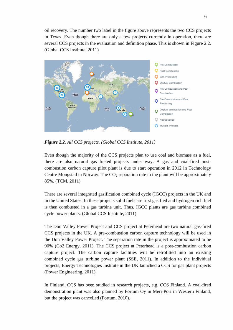
oil recovery. The number two label in the figure above represents the two CCS projects
in Texas. Even though there are only a few projects currently in operation, there are
several CCS projects in the evaluation and definition phase. This is shown in Figure 2.2.
(Global CCS Institute, 2011)
Figure 2.2. All CCS projects. (Global CCS Institute, 2011)
Even though the majority of the CCS projects plan to use coal and biomass as a fuel,
there are also natural gas fueled projects under way. A gas and coal-fired post-
combustion carbon capture pilot plant is due to start operation in 2012 in Technology
Centre Mongstad in Norway. The CO2 separation rate in the plant will be approximately
85%. (TCM, 2011)
There are several integrated gasification combined cycle (IGCC) projects in the UK and
in the United States. In these projects solid fuels are first gasified and hydrogen rich fuel
is then combusted in a gas turbine unit. Thus, IGCC plants are gas turbine combined
cycle power plants. (Global CCS Institute, 2011)
The Don Valley Power Project and CCS project at Peterhead are two natural gas-fired
CCS projects in the UK. A pre-combustion carbon capture technology will be used in
the Don Valley Power Project. The separation rate in the project is approximated to be
90% (Co2 Energy, 2011). The CCS project at Peterhead is a post-combustion carbon
capture project. The carbon capture facilities will be retrofitted into an existing
combined cycle gas turbine power plant (SSE, 2011). In addition to the individual
projects, Energy Technologies Institute in the UK launched a CCS for gas plant projects
(Power Engineering, 2011).
In Finland, CCS has been studied in research projects, e.g. CCS Finland. A coal-fired
demonstration plant was also planned by Fortum Oy in Meri-Pori in Western Finland,
but the project was cancelled (Fortum, 2010).

7
3 CO2 CAPTURE
The production of CO2 cannot be avoided when hydrocarbon fuels are combusted. To
reduce CO2 emissions, carbon has to be captured. The purpose of CO2 capture is to
produce a concentrated stream of CO2 at high pressure that can be transported to a
storage site. (Rackley, 2010; VTT 2010)
There are currently three primary technologies to reduce CO2 emissions. The
technologies which decarbonize the fuel prior to combustion are known as pre-
combustion technologies. In technologies know as post-combustion, CO2 is separated
from flue gases. Combustion can also be re-engineered in such a way that it produces
only CO2 and water that can be condensed after combustion. This capture technology is
called oxy-fuel combustion. In oxy-fuel combustion the fuel is combusted in pure
oxygen. There is also significant modification of oxy-fuel combustion, known as
chemical looping. (Rackley, 2010; VTT 2010)
A number of technologies to separate CO2 from other gases have been studied. In post-
and pre-combustion technologies the technologies are absorption, adsorption, membrane
and cryogenic technologies. In oxy-fuel capture technology the CO2 is separated from
steam, as the exhaust gases consist of only CO2 and steam after combustion with
oxygen. The oxygen required is separated from air. These separation technologies
include adsorption, membranes and cryogenic technologies. (Rackley, 2010; VTT 2010)
The CO2 capture technologies are introduced in chapters 3.1, 3.2 and 3.3. In addition,
these chapters evaluate the strengths, weaknesses, opportunities and threats (SWOT
analysis). SWOT-analysis is a strategic management tool. It helps to evaluate the
attractiveness of the business field or, as in this case, the technology. (Haverila et al,
2005).
Transportation and storage of CO2 is briefly introduced in chapter 3.4. The capture
technologies are compared in chapter 3.5.
3.1 Post-combustion
In post-combustion CO2 capture technology the CO2 is separated from the flue gases.
The main component is typically nitrogen. In this manner, the separation technologies
are developed to separate CO2 from N2. The technologies used in separation are already
used in a wide range of industrial processes, refining and gas processing. Thus, the

8
technology in itself is mature, but not in CCS usage. However, post-combustion is the
most mature CO2 capture system in the power sector. It can be considered as an
extension of the fuel gas treatment for other emissions. Figure 3.1 presents the block
diagram for post-combustion CO2 capture in CCGT. (IEA, 2008; Rackley 2010)
Figure 3.1. Block diagram for post-combustion CO2 capture.
Numerous demonstration projects are expected to use the chilled ammonia process. The
research, development and demonstration projects currently focus on new solvents that
would consume less energy and reduce the cost of CO2 capture. Other focuses are on
integration of CCS within the power plant and on the procedures for optimal operation
under varying plant conditions. (Rackley, 2010; IEA, 2008)
Table 3.1 presents the SWOT analysis for post-combustion technology. As mentioned
earlier, the strongest strength of post-combustion technology lies in the maturity of the
technology.
Table 3.1. Post-combustion SWOT (Racley, 2010; VTT, 2010; IPCC, 2005; Damen
et al, 2006)
Strengths
Fully developed technology,
commercially deployed at the scale
in other industry sectors
Simple technology
Weaknesses
High energy demand for
regenerating the solvent
May demand significant amounts
of process water
Opportunities
Retrofit to existing plant
Capture readiness
Threats
Slippage of solvent may become a
health, safety and environmental
issue
NGPower and heat
production
Flue gas
cleaning
CO2
captureAir
CO2 conditioning
and compression
Cleaned
exhaust
Transportation
to storage
CO2

9
3.2 Pre-combustion
Pre-combustion technologies are used commercially in various industrial applications,
such as the production of hydrogen and ammonia. Figure 3.2 presents the block diagram
for pre-combustion CO2 capture in CCGT. In a natural gas fueled power plant the fuel
must be reformed and sifted to generate a mixture of hydrogen and CO2. Then, either
the CO2 is removed using sorbents or the hydrogen is removed using membranes.
Separation of CO2 from H2 is easier than from N2 due to the greater difference between
molecular weights and molecular kinetic diameters. (IEA, 2008; Rackley 2010)
Figure 3.2. Block diagram for pre-combustion CO2 capture.
Currently, the most promising pre-combustion technologies use physical solvents. In
physical absorption the bond is much weaker between CO2 and the solvent than in the
chemical absorption. Bonding takes place at high pressure and the CO2 is released again
when the pressure is reduced. Energy is needed to drive the compressors for gas
pressurization in the separation system. The energy conversation of the capture
technology is higher when the concentration of CO2 in the flue gases is lower. (IEA,
2008; Rackley, 2010)
The SWOT analysis for the pre-combustion CO2 capture technology is presented in
Table 3.2. The relatively low need of energy in the CO2 separation is the strongest
strength of the pre-combustion technology.
NGReformer
Water-Gas-
Shift
CO2 capture
(H2 separator)
H2-rich fuelAir/SteamPower and heat
productionFlue
gases
CO2 conditioning
and compression
Transportation
to storageCO2
Air

10
Table 3.2. Pre-combustion SWOT (Racley, 2010; VTT, 2010; IPCC, 2005; Damen
et al, 2006)
Strengths
Relatively high CO2 concentration
before separation lower energy
demand for CO2 capture and
compression
When increasing CO2 capture rate,
the specific energy requirement
does not greatly increase
Separation of CO2 from H2 is
easier than from N2
Weaknesses
Temperature and efficiency issues
associated with hydrogen-rich gas
turbine fuel
Increase of NOx emissions due to
increased flame temperature
Opportunities
Development of H2 fueled gas
turbine
High development potential owing
to the combined power cycle
Threats
Difficult to retrofit
Complex technology has to be used
3.3 Oxy-fuel Combustion
The oxy-fuel process involves the combustion of hydrocarbons in almost pure oxygen,
obtained from an air separator unit. Because of different combustion characteristics a
different approach to air combustion is required, such as water recycling or flue gas
recycling. (IEA, 2008)
The block diagram for oxy-fuel combustion CO2 capture technology is presented in
Figure 3.3. First, the oxygen is separated from the air, which is used to burn natural gas.
The flue gases from the combustion contain mainly water and CO2. Part of the flue
gases is recycled back to the process and part of it is conducted to CO2 separation. The
CO2 is separated by condensing the water in the flue gases.

11
Figure 3.3. Block diagram for oxy-fuel combustion CO2 capture
Chemical looping is a promising variant of oxy-fuel capture technology. In this process,
calcium compounds or metal compounds are used to carry oxygen and heat between
successive reaction loops. In the gas turbine application the fuel oxidation reactor
replaces the conventional combustion chamber. The CO2 is separated as in regular oxy-
fuel technology. Chemical looping is still at a very early stage of development and has
been the subject of laboratory-scale experiments. (IEA, 2008; Rackley 2010)
The SWOT analysis for the oxy-fuel combustion system, which includes chemical
looping is presented in Table 3.3. In the table chemical looping is regarded as a
development opportunity in oxy-fuel combustion.
Table 3.3. Oxy-fuel combustion SWOT (Racley, 2010; VTT, 2010; IPCC, 2005;
Damen et al, 2006)
Strengths
Mature air separation technologies
available
Weaknesses
Least mature technology
Production of oxygen consumes
energy and is expensive
Opportunities
Chemical looping
Combination with other capture
systems
Threats
Difficult to retrofit
Power and heat
production
Air
separatorAir
O2
N2
NG Flue gas
recycling
Water
condensing
CO2 conditioning
and compression
Transportation
to storage
CO2
H2O

12
3.4 CO2 Separation
The most advanced CO2 separation technology is chemical absorption. Other currently
studied separation technologies are physical absorption, physical and chemical
adsorption, membrane separation, and cryogenic and distillation. (Rackley, 2010)
In chemical absorption, chemical compounds between the solvent and CO2 are formed
in an absorber. The distillate is released from the top of the absorber tower and the CO2
rich solvent from the bottom. The absorption reaction is exothermic. In an exothermic
reaction energy is released. The reaction is then reversed in the stripping process, which
requires heat. In physical absorption, chemical compounds are not formed. The solvent
in physical absorption is chemically inert and absorbs the CO2 without a chemical
reaction. (Rackley, 2010)
The difference to absorption in adsorption CO2 lies in the surface of the sorbent. In
absorption it enters the solvent. In both absorption and adsorption of CO2 a chemical
bond or a weaker physical attractive force can be formed. (Rackley, 2010)
Membranes separate CO2 from gas stream by filtering. The filtering process can involve
a number of different physical and chemical processes. The key characteristic of
membranes is the porosity. They can be either porous or non-porous. In porous
membranes, a permeate is transported through the membrane by molecular sieving. In
non-porous, the transport mechanism is called a solution-diffusion. (Rackley, 2010)
Cryogenic separation technology is based on distillation. In distillation, the separation
of a mixture of liquids into its components depends upon the difference in the boiling
points and volatilities of the components. (Rackley, 2010)
3.5 CO2 Transportation and Storage
Captured CO2 has to be transported to the storage site. The transportation cost has a
strong impact on the overall cost of CCS. Distances from a power plant to a potential
geological storage site can be up to 1,000–1,500 km in Finland (VTT, 2010).
The transportation methods that have received attention in the literature are pipeline and
ship transportation. Other transportation methods do not have sufficient capacity to
transport the amount of CO2 captured from a power plant. Transportation of CO2 by
pipeline is a mature technology. It has been in use in enhanced oil recovery in the
United States since the 1970’s. The factors that affect the cost and safety of pipeline
transportation are well known. (VTT, 2010)

13
At the storage location, CO2 has to be stored for several thousand years in isolation from
the atmosphere. The long storage time adds an uncertainty to all storage technologies.
Because of the large amount of CO2, there are only few possible storage options. To
date, only storage in underground geological formation has been demonstrated on a
large scale. These geological formations are, for example, oil fields or gas fields. (VTT,
2010)
Another promising storage option is mineral carbonization. Mineral carbonization is
binding the CO2 with silicate minerals into solid carbonates. Currently, is it not viable
because of its high energy consumption. (VTT, 2010)
One of the difficulties in transportation and storage of CO2 is the lack of international
regulations. However, the EU has implemented a directive concerning CO2 storage
within the EU. According to the directive, a permit is required for storage. The
operating party remains responsible for storage site monitoring, maintenance and
reporting also after the storage site is closed. The directive also requires that the purity
of the CO2 stream is high. (EU, 2009) Possible storage locations for CO2 produced in
Finland are in Norway (VTT, 2011). Even though Norway is not part of the EU, it can
be assumed to have similar regulations.
3.6 Comparison of CO2 Capture Technologies
The technology for the case study of the thesis has been chosen by comparing the
technologies from a new CCGT CHP plant perspective. Important factors in the
comparison are net plant efficiency and maturity of the technology. The SWOT
analyses presented in previous subchapters have also influenced the decision. Because
the thesis is part of a larger project, the demands of the project have also been taken into
account when selecting the case.
According to the results of the SWOT analysis in chapter 2, pre-combustion technology
seems appealing from the new CCGT CHP plant perspective. Pre-combustion
technologies are mainly more mature than oxy-fuel technologies. In the pre-combustion
cases, the energy penalties are lower than in post-combustion cases. The VTT’s report
also mentions that the development potential in pre-combustion is high in combined
cycle applications. (VTT, 2010; Rackley, 2010; IPCC, 2005; Damen et al, 2006)
The separation technologies used in capture systems are presented in the Table 3.4. The
table provides an overview of all the separation techniques studied. (Rackley, 2010;
VTT 2010)

14
Table 3.4. Separation technologies. (Rackley, 2010)
Post-combustion
CO2 separation from
N2
Pre-combustion
CO2 separation from
H2
Oxy-fuel combustion
O2 separation from N2
Absorption Chemical solvents
(e.g. MEA, chilled
ammonia)
Physical solvents (e.g.
Selexol, Fluor
process), Chemical
solvents
Adsorption Zeolite and activated
carbon molecular
sieves, Carbonate
sorbents, Chemical
looping
Zeolite, Activated
carbon, Hydrotalcites
and silicates
Zeolite and activated
carbon molecular
sieves, Perovskites and
chemical looping
Membranes Polymeric
membranes,
Immobilized liquid
membranes, Molten
carbonate membranes
Metal membrane
WGS reactors, Ion
transport membranes
Polymeric membranes,
Ion transport
membranes, Carbon
molecular sieves
Cryogenic CO2 liquefaction,
Hybrid cryogenic +
membranes
CO2 liquefaction,
Hybrid cryogenic +
membranes
Distillation
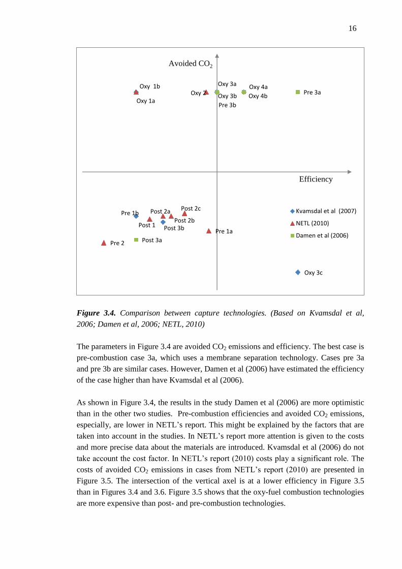
The results of three different studies comparing CO2 capture technologies are presented
in Figure 3.4. The red triangles are from NETL’s report (2010), the green squares are
from Damen et al (2006), and the blue diamonds are from Kvamsdal et al (2006). Even
though the Kvamsdal et al (2006) article referred to here was published about the same
time as the Damen et al (2006) article, Damen et al uses as a reference an earlier
presentation from Kvamsdal et al (2004), which is almost the same as Kvamsdal et al
(2006). NETL’s report (2010) uses both Damen et al (2006) and Kvamdal et al (2007)
as references. Below are the explications for the designations in the figure.
15
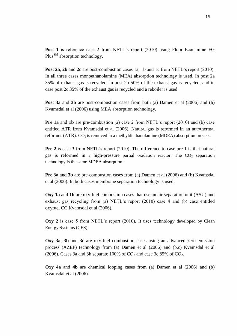
Post 1 is reference case 2 from NETL’s report (2010) using Fluor Econamine FG
PlusSM
absorption technology.
Post 2a, 2b and 2c are post-combustion cases 1a, 1b and 1c from NETL’s report (2010).
In all three cases monoethanolamine (MEA) absorption technology is used. In post 2a
35% of exhaust gas is recycled, in post 2b 50% of the exhaust gas is recycled, and in
case post 2c 35% of the exhaust gas is recycled and a reboiler is used.
Post 3a and 3b are post-combustion cases from both (a) Damen et al (2006) and (b)
Kvamsdal et al (2006) using MEA absorption technology.
Pre 1a and 1b are pre-combustion (a) case 2 from NETL’s report (2010) and (b) case
entitled ATR from Kvamsdal et al (2006). Natural gas is reformed in an autothermal
reformer (ATR). CO2 is removed in a methyldiethanolamine (MDEA) absorption process.
Pre 2 is case 3 from NETL’s report (2010). The difference to case pre 1 is that natural
gas is reformed in a high-pressure partial oxidation reactor. The CO2 separation
technology is the same MDEA absorption.
Pre 3a and 3b are pre-combustion cases from (a) Damen et al (2006) and (b) Kvamsdal
et al (2006). In both cases membrane separation technology is used.
Oxy 1a and 1b are oxy-fuel combustion cases that use an air separation unit (ASU) and
exhaust gas recycling from (a) NETL’s report (2010) case 4 and (b) case entitled
oxyfuel CC Kvamsdal et al (2006).
Oxy 2 is case 5 from NETL’s report (2010). It uses technology developed by Clean
Energy Systems (CES).
Oxy 3a, 3b and 3c are oxy-fuel combustion cases using an advanced zero emission
process (AZEP) technology from (a) Damen et al (2006) and (b,c) Kvamsdal et al
(2006). Cases 3a and 3b separate 100% of CO2 and case 3c 85% of CO2.
Oxy 4a and 4b are chemical looping cases from (a) Damen et al (2006) and (b)
Kvamsdal et al (2006).
16
Figure 3.4. Comparison between capture technologies. (Based on Kvamsdal et al,
2006; Damen et al, 2006; NETL, 2010)
The parameters in Figure 3.4 are avoided CO2 emissions and efficiency. The best case is
pre-combustion case 3a, which uses a membrane separation technology. Cases pre 3a
and pre 3b are similar cases. However, Damen et al (2006) have estimated the efficiency
of the case higher than have Kvamsdal et al (2006).
As shown in Figure 3.4, the results in the study Damen et al (2006) are more optimistic
than in the other two studies. Pre-combustion efficiencies and avoided CO2 emissions,
especially, are lower in NETL’s report. This might be explained by the factors that are
taken into account in the studies. In NETL’s report more attention is given to the costs
and more precise data about the materials are introduced. Kvamsdal et al (2006) do not
take account the cost factor. In NETL’s report (2010) costs play a significant role. The
costs of avoided CO2 emissions in cases from NETL’s report (2010) are presented in
Figure 3.5. The intersection of the vertical axel is at a lower efficiency in Figure 3.5
than in Figures 3.4 and 3.6. Figure 3.5 shows that the oxy-fuel combustion technologies
are more expensive than post- and pre-combustion technologies.
Post 3b
Pre 1b
Oxy 1b
Oxy 4b Oxy 3b
Pre 3b
Oxy 3c
Post 1
Post 2a
Post 2b
Post 2c
Pre 1a
Pre 2
Oxy 1a Oxy 2
Post 3a
Pre 3a Oxy 4a Oxy 3a
Kvamsdal et al (2007)
NETL (2010)
Damen et al (2006)
Efficiency
Avoided CO2

17
Figure 3.5. Cost of avoided CO2 emissions (Based on NETL, 2010)
In addition to the factors mentioned above, the maturity of the technology is an
important factor when selecting the case for the modeling part of the thesis. In NETL’s
report (2010) all the cases, except case post 1 (reference case 2 in NETL’s report), are
estimated to need 6–10 years of development. Case post 1 has already been
demonstrated. Figure 3.6 presents the maturity of the cases from Kvamsdal et al (2006).
As shown in Figure 3.6, the most mature technologies have the lowest efficiency. There
can be at least two explanations for this trend. First, it can be assumed that the
development of the technologies with better efficiency has started later, and that is why
they are still at an earlier development stage. Another reason for the trend might be that
as development progresses, the realities have to be taken into account and more factors
appear, which lowers the efficiency.
The three studies compared above support the result from the SWOT analysis. The
results favor the selection of pre-combustion technology for analysis in the case study.
Because it is important for the thesis to have reliable information about the chosen
technology, a mature pre-combustion technology has been chosen.
Efficiency
Cost of Avoided
CO2 Emission

18
Figure 3.6. Level of maturity. (Prepared based on Kvamsdal et al, 2006)
The most mature pre-combustion technology involves an ATR reactor. Air-blown ATR
reactors are well suited to integration with a combined cycle for two reasons. First, air
entering the ATR can be extracted from the gas turbine compressor. Second, final fuel is
diluted with nitrogen, which reduces the NOx emissions to an acceptable level. This
reduces the previously mentioned weakness that pre-combustion technologies have.
(Corradetti and Desideri, 2005)
Amine ATR
Oxy fuel CC
CLC
AZEP 100%
MSR-H2
AZEP 85%
Efficiency
Level of
maturity

19
4 ENERGY ECONOMICS
The main principles of energy economics are introduced first in this chapter. Later in
the chapter, calculation methods used in the thesis are presented.
The American Association of Cost Engineers defines cost engineering as “the area of
engineering practice where engineering judgment and experience are used in the
application of scientific principles and techniques to problems of business and program
planning, cost estimating, economic and financial analysis, cost engineering, program
and project management, planning and scheduling, cost and schedule performance
measurement, and change control”. The list of practice areas is collectively called cost
engineering, while the process through which these practices are applied is called total
cost management or TCM. (AACE, 2011)
Neilimo and Uusi-Rauva (2007) define the role of cost engineering to ensure affordable
realization of a project. This includes cost estimating, project budgeting, schedule and
cost optimization, cash flow calculations, cost reporting and control decisions. As in all
projects, energy projects, too, are dominated by scarcity, unless they are designated for
a demonstrative or experimental purpose. Scarcity refers to an economic problem or to
having limited resources. (Neilimo & Uusi-Rauva, 2007; Vanek, 2008)
The economics of energy production includes the initial cost of the components of the
power plant, operating costs, and the price of electricity and heat when sold on the
markets. The cost of the components of the power plant and part of the operating costs,
e.g. wages, constitute the fixed costs of the power plant. The remainder of the operating
costs, e.g. fuel, are called variable costs. Variable costs depend on the operating rate, on
which fixed costs do not depend. The major factors that influence the costs are
government incentives, capital costs which include construction costs and financing,
fuel costs, and air emissions controls for coal and natural gas plants. The relationship
between power plant investment and society’s collective choices is important because
excessive investment or underinvestment can both lead to higher energy costs for the
public. (Kaplan, 2008; Vanek, 2008)
The demand for electricity and heat is not constant. The operating time of the plant
depends on the demand it is planned to meet. Duration curves (see Figure 4.1) illustrate
how much electricity is needed and for how long. Base load power plants operate
almost all the time at full load. The best example of a base load plant is a nuclear power
plant. Its high investment cost and low operating costs support the high peak load hours.

20
A CCGT power plant can be used as intermediate load and base load power plants. The
investment cost for a CCGT plant is relatively low and partial load use is possible. The
main features of peak load power plants are low investment cost and high operation
cost. An example of a peak load power plant is a diesel generator. (Kehlhofer et al,
1999)
Figure 4.1. Load duration curve. (National Grid, 2006)
There are many methods to estimate the cost of a power plant investment. For example,
the cost can be roughly estimated by size or some other rule of thumb method (Neilimo
& Uusi-Rauva, 2007). Cost estimation methods and accuracies are presented in
Appendix 1. In the table the estimation methods are categorized by the phase of the
estimation cycle. The table is used in estimating the accuracy of the calculations. In the
thesis, the power plant is hypothetical and not all the data needed for a complete cost
estimation is available. Thus, many assumptions are made. Only the magnitude of the
costs can be calculated.
4.1 Efficiency and Power-to-Heat Ratio
The efficiency of the power plant is a major factor influencing the costs of produced
energy. The investment cost of the power plant strongly influences its feasibility,
especially when the operation rate is low. However, the core factors are usability and
efficiency. Besides operation hours, failures and availability also affect usability. (IFRF,
2002)
Good efficiency is not only an economic factor. Improvement in efficiency also lowers
the emissions. The better the efficiency, the more energy can be produced with the same

21
amount of fuel. From a cost point of view, efficiency could be calculated strictly as the
ratio of energy sold to the fuel purchased in energy units in a specific time range.
(Equation 1)
where ηtot is the overall efficiency of the power plant. It is assumed that all electricity
that is not consumed by the plant can be power sold on the power markets.
Overall efficiency of the power plant will be calculated in the thesis as shown in
equation (1). In the thesis, the auxiliary electricity consumption is subtracted from the
total produced electricity. Also the heat produced to the reformer and absorber
(explained in detail in chapter 5.2) is not calculated in the heat power output.
The advantage of presenting efficiency, as in equation (1), is that it represents how well
the fuel can be converted into products to be sold. If the efficiency increases, more heat
and power can be produced with the same amount of fuel. Conversely, more fuel is
needed to produce the same amount of heat and power if the efficiency decreases.
However, efficiency cannot be increased endlessly. Higher efficiency usually requires
more expensive equipment.
Besides investment cost and efficiency, another interesting factor influencing the
feasibility of the power plant is the power to heat ratio. However, if the prices of heat
and electricity are almost the same, power to heat ratio has no effect. The equation for
the power to heat ratio is presented in equation (2). The same values of electricity and
heat are used as in the energy efficiency equation.
(Equation 2)
Both power and heat are forms of energy converted from the energy of the fuel. Energy
efficiency represents how well this can be done. However, energy efficiency does not
differentiate between the values of these energies. The value of the energy represents
how well the form of energy can be converted into another form. For example,
electricity can be converted into heat almost with 100% efficiency, but heat cannot be
converted into electricity as efficiently. This value of energy is called exergy. (VTT,
2004)
Heat and power production is worth combining when its cost is lower than producing
them separately. Because the advantage is achieved by combining the productions, it is
logical to require that the advantage is divided for both heat and power. The guideline
for the division of the advantage should not exceed the costs of alternative electricity

22
production that is not combined with heat production, and vice versa, should not exceed
the cost of alternative heat production costs. (VTT, 2004)
In addition to the guideline described above, there are many ways to divide the
advantage gained from combined production. For example, the advantage can be
divided based on the amount of energy or exergy, the ratio between the costs of the
separate productions, or the ratio between the prices of electricity and heat. (VTT, 2004)
The method used in the thesis is based on the energy method. However, the proportion
of costs allocated to heat is the produced heat multiplied by 0.9. The remainder of the
costs are allocated to electricity. This is due to the tax regulations. The proportion of
natural gas that is used in electricity production is tax-free. Taxes have to be paid on the
proportion that is used in heat production. In Finnish regulations, the proportion of
natural gas on which taxes have to be paid is the heat produced multiplied by 0.9
(Tullihallitus, 2011). To ensure the coherence of the methods, this coefficient is also
used in cost allocation.
4.2 Feasibility of the Investment
There are many ways to compare investment feasibility. In the net present value (NPV)
method, all elements of the financial analysis are discounted back to their present worth.
The internal rate of return (IRR) indicates the rate of return when the net present value
is zero. The return on invest (ROI) method is a simplified version of IRR. ROI is
calculated by dividing the profit of a typical year by the investment. The annuity
method can be considered as a reversed NPV method because it divides the investment
cost equally for the years the investment is operative. The payback time method
calculates the length of the payback time for the investment. (Neilimo & Uusi-Rauva,
2007; Vanek & Louis, 2008)
In the thesis, the net present value method is used in investigating the feasibility of the
invetment. NPV is chosen because it gives a simple limit for the feasibility of the
investment. The changes in feasibility can easily be investigated by keeping the NPV as
zero and changing variables affecting it. It takes into account all the parameters needed
in the case and is easy to calculate. Net present value is calculated by adding together all
the revenues and costs incurred by the investment in present value. If the net present
value is positive, the investment is feasible. The present values are calculated with a
present values factor. The present value factor is calculated from the interest rate as
follows:
(Equation 3)
23
where d is present value factor, i is interest rate, and n is the year when the cost or
revenue is expected. (Neilimo & Uusi-Rauva, 2007)
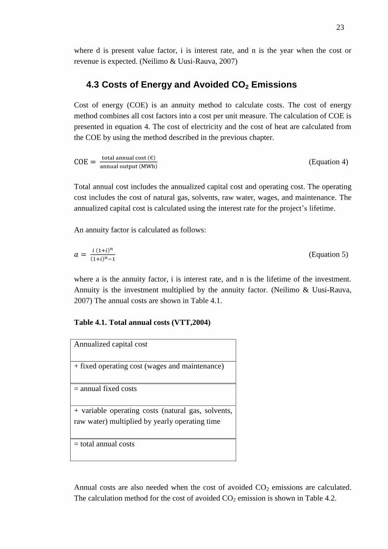
4.3 Costs of Energy and Avoided CO2 Emissions
Cost of energy (COE) is an annuity method to calculate costs. The cost of energy
method combines all cost factors into a cost per unit measure. The calculation of COE is
presented in equation 4. The cost of electricity and the cost of heat are calculated from
the COE by using the method described in the previous chapter.
(Equation 4)
Total annual cost includes the annualized capital cost and operating cost. The operating
cost includes the cost of natural gas, solvents, raw water, wages, and maintenance. The
annualized capital cost is calculated using the interest rate for the project’s lifetime.
An annuity factor is calculated as follows:
(Equation 5)
where a is the annuity factor, i is interest rate, and n is the lifetime of the investment.
Annuity is the investment multiplied by the annuity factor. (Neilimo & Uusi-Rauva,
2007) The annual costs are shown in Table 4.1.
Table 4.1. Total annual costs (VTT,2004)
Annualized capital cost
+ fixed operating cost (wages and maintenance)
= annual fixed costs
+ variable operating costs (natural gas, solvents,
raw water) multiplied by yearly operating time
= total annual costs
Annual costs are also needed when the cost of avoided CO2 emissions are calculated.
The calculation method for the cost of avoided CO2 emission is shown in Table 4.2.

24
Table 4.2. Cost of avoided CO2 emissions.
Total annual costs
– Total annual costs in reference plant
Difference in total annual costs
/ The amount of avoided CO2 emissions
Cost of avoided CO2 emissions
Emissions are also calculated per heat or electricity produced. In the case of heat, all the
CO2 emissions are divided by the heat produced. Correspondingly, in the case of
electricity, all CO2 emissions are divided by the electricity produced.

25
5 POWER PLANT ASSUMPTIONS
The power plant models are introduced in this chapter. Both CCGT CHP with and
without CO2 capture are modeled. The power plant without CO2 capture is modeled
with Solvo ®, presented in chapter 5.3.
The power plant with CO2 capture is built with three programs. This is presented in
chapters 5.1 and 5.2. The base components of the power plant are modeled with Solvo
®. The reforming process is modeled with Microsoft Excel ®. The absorption system is
modeled with Aspen Plus ®. The limits and integration between the programs are
presented in Figure 5.1. The diagrams of the model from the modeling programs Solvo
® and AspenPlus ® are presented in appendices 2 and 3, respectively.
Figure 5.1. Power plant model.
The model and the assumptions made in modeling are presented in this chapter. The
assumptions are based on the literature and information available in the programs. Solvo
® is a power plant design and optimization tool developed by Fortum Oyj (Fortum,
2011). Aspen Plus ® is a process tool for design, optimization and performance
monitoring for the chemical, polymer, specialty chemical, metals and minerals and coal
Natural gas reforming
Absorber
Gas turbine
Heat recovery steam
generator
District heating
Process steam and water
Process water
Synthetic gas
Exhaust gases
SOLVO ®
AspenPlus ®
MS Excel ®
CO2 compression
CO2
Synthetic gas
Process
water
Steam turbine
Electricity
Electricity
Heat
Exhaust gases
Natural gas
Solvents
CO2
Process steam
Process steamProcess steam
Process steam
Added water
AspenPlus ®

26
power industries (Aspen Tech, 2011). Microsoft Excel is a tool to create and format
spreadsheets (Microsoft, 2011).
5.1 Combined Cycle Gas Turbine Power Plant
The combined cycle gas turbine power plant modeled is introduced in this chapter. The
system consists of two gas turbines, two heat recovery steam generators, and one steam
turbine. The fuel used is natural gas that is reformed in a natural gas reformer. The heat
load is 350 MW. The power plant is located by the sea, thus cooling water is always
available.
5.1.1 Fuel – Natural Gas
Natural gas used in Finland comes from West-Siberia’s natural gas fields. The
formulation and properties of the gas is shown in Table 5.1. The values in Table 5.1 are
average values from measured values in 1 October 2004–31 May 2011 (Gasum, 2011).
Table 5.1. Formulation and properties of natural gas used in Finland. (Based on
Gasum, 2011)
Formulation mol-% M (g/mol)
CH4 98.09 16.04
C2H6 0.76 30.07
C3H8 0.28 44.10
C4H10 0.08 54.09
C5H12 0.01 72.15
N2 0.79 28.01
CO2 0.04 44.01
Lower Heat Value q 36.01 MJ/m3
Higher Heat Value qp 39.94 MJ/m3
Density ρ 0.73 kg/m3n
Molar Mass M 16.35 g/mol

27
When natural gas is combusted in air, the combustion reaction are as follows:
CH4 + 2 O2 + 7.54 N2 → CO2 + 2 H2O + 7.54 N2 (Reaction 1)
C2H6 + 3.5 O2 + 13.195 N2 → 2 CO2 + 3 H2O + 13.165 N2 (Reaction 2)
C3H8 + 5 O2 + 18.85 N2 → 3 CO2 + 4 H2O + 18.85 N2 (Reaction 3)
C4H10 + 6.5 O2 + 24.51 N2 → 4 CO2 + 5 H2O + 24.51 N2 (Reaction 4)
C5H12 + 8 O2 + 30.16 N2 → 5 CO2 + 6 H2O + 30.16 N2 (Reaction 5)
(0.981 CH4 + 0.008 C2H6 + 0.003 C3H8 + 0.001 C4H10 + 0.008 N2) + 2.01 O2 + 7.58 N2
→ 1.01 CO2 + 2.00 H2O + 7.58 N2 (Reaction 6)
In stoichiometric combustion, 1 mol of natural gas requires 9.59 mol of dry air.
In pre-combustion capture technologies natural gas is reformed and H2 is combusted
with air in combustion chambers. A small fraction of natural gas is combusted in an
auto-thermal reformer, which is presented in chapter 5.2.1.
5.1.2 Gas Turbine
The gas turbine modeled is based on a real machine, Siemens V 94.2. The turbine is
chosen because it can be converted to synthetic gas combustion (Siemens, 2011). It is
assumed here that the modifications that have to be made to the gas turbine for
hydrogen rich combustion will not affect the performance of the gas turbine.
The parameters of the Siemens V 94.2 gas turbine are built in the Solvo ® program in a
gas turbine unit. The fuel-to-gas turbine in the Solvo ® model comes from the fuel tank
unit. The fuel is defined as natural gas, but the composition of the fuel is changed to
correspond to the CO2 lean synthetic gas from the CO2 removal unit. The CO2 removal
unit is modeled with Aspen Plus ®, which is presented in chapter 5.2.2. Figure 5.2
presents a block diagram for the gas turbine unit.
Figure 5.2. Gas turbine unit.
Gas Turbine Unit
Synthetic Gas
AirExhaust Gases

28
Air compressed in the gas turbine unit is conducted to the combustion chamber. In the
combustion chamber, H2 rich fuel (synthetic gas) is combusted with air and the exhaust
gases are conducted to the turbine section of the gas turbine unit. There are two gas
turbine units in the modeled power plant. Exhaust gases from the gas turbines are
conducted to heat recovery steam generators (HRSG). These two combined gas turbine
– HRSG units are identical.
5.1.3 Heat Recovery Steam Generator (HRSG)
Two HRSGs are placed after the gas turbines, one after each turbine. Hot exhaust gases
from the gas turbines are conducted through the HRSG. Heat from the exhaust gases is
transferred to process water, district heating water, and synthetic gas in the HRSG. A
simplified block diagram of the HRSG is presented in Figure 5.3.
Figure 5.3. Heat recovery steam generator.
The key to the abbreviations in Figure 5.3 are as follows: HPS (high pressure steam),
ST (steam turbine), REF (natural gas reformer), HPW (high pressure water), LPS (low
pressure steam), LPW (low pressure water), DHW (district heating water) and EG
(exhaust gases).
Part of process water heating takes place in the synthetic gas production section (see
chapter 5.2.1). Process steam generation is highly integrated between the HRSG and
synthetic gas production section, which also provides heat. The high pressure level is 90
bar, and the low pressure level 7 bar in full load. In partial load, a flexible pressure is
used.
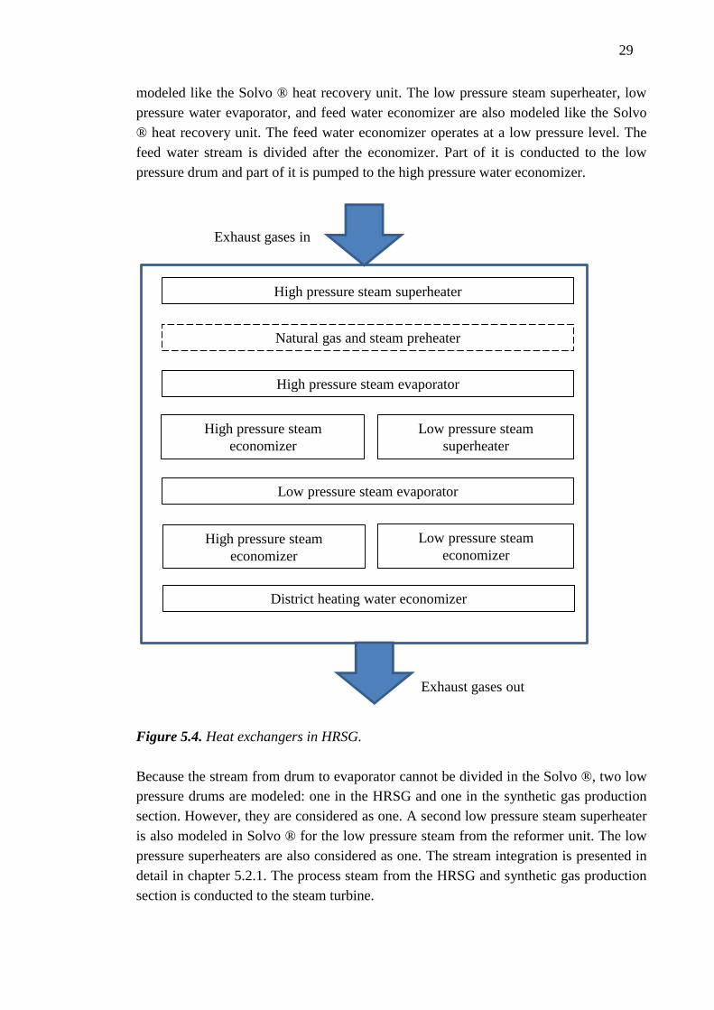
In the Solvo ® model, the heat exchangers are arranged as in Figure 5.4. Steam for the
high-pressure steam superheater comes from a superheater in the reformer unit. The
high-pressure superheater is modeled like the Solvo ® superheater unit. The synthetic
gas preheater is modeled like the reheater unit. It only models the heat consumption of
the preheater in the HRSG. The high-pressure water economizer and evaporator are
Heat Recovery Steam Generator
DHW
DHW
Feed Water
LPW to
REF
LPS from
REF
LPS to ST
HPS to
REF
HPS from
REF
HPS to ST
EG EG
HPW to
REF
HPW from
REF
29
modeled like the Solvo ® heat recovery unit. The low pressure steam superheater, low
pressure water evaporator, and feed water economizer are also modeled like the Solvo
® heat recovery unit. The feed water economizer operates at a low pressure level. The
feed water stream is divided after the economizer. Part of it is conducted to the low
pressure drum and part of it is pumped to the high pressure water economizer.
Figure 5.4. Heat exchangers in HRSG.
Because the stream from drum to evaporator cannot be divided in the Solvo ®, two low
pressure drums are modeled: one in the HRSG and one in the synthetic gas production
section. However, they are considered as one. A second low pressure steam superheater
is also modeled in Solvo ® for the low pressure steam from the reformer unit. The low
pressure superheaters are also considered as one. The stream integration is presented in
detail in chapter 5.2.1. The process steam from the HRSG and synthetic gas production
section is conducted to the steam turbine.
High pressure steam evaporator
Low pressure steam evaporator
High pressure steam
economizer
Low pressure steam
superheater
Low pressure steam
economizer
High pressure steam superheater
High pressure steam
economizer
District heating water economizer
Natural gas and steam preheater
Exhaust gases in
Exhaust gases out

30
5.1.4 Steam Turbine
There is one steam turbine in the model. Steam from both HRSGs and from the
synthetic gas production section is conducted to the one steam turbine. There are five
steam extractions from the steam turbine. Medium pressure steam (MPS) from the first
extraction is conducted to the reforming process (REF) in 25 bar, which is the pressure
of natural gas supplied to the power plant. From the second extraction the steam is
conducted to the feed water tank (FWT) at 3.5 bar. The third extraction is to the CO2
separation unit (ABS) at 0.63 bar. From the last two extractions the steam is conducted
to the district heating water heat exchangers (DH). The remainder of the steam expands
at the end of the steam turbine to a pressure of 0.02 bar and is conducted to a condenser
(COND). The block diagram for the steam turbine unit, the condenser and the feed
water tank is presented in Figure 5.5.
In Solvo ® the steam turbine consists of 7 separate steam turbine units linked to each
other with a shaft. High pressure steam (HPS) is conducted to the first turbine from
which the first extraction is taken. Low pressure steam (LPS) is conducted to the third
turbine unit. In the first and second steam turbines the isentropic efficiency is 0.90 and
in the remaining steam turbines 0.85.
Figure 5.5. Steam turbine, condenser and feed water tank.
5.1.5 District Heating
The power plant has two heat exchangers for district heating water. The district heat
consumption is the main parameter influencing the plant size. The ccold district heating
Steam Turbine
MPS to REF LPS to
abs
LPS to
DH
LPS to
DH
LPS to
FWT
HPS from
HRSG
LPS from
HRSG
CondenserFeed Water TankFW to HRSG
Water from ABS
Add. water

31
water stream is divided into two streams. One stream is conducted to the HRSG and one
to the low temperature heat exchanger. After the low temperature heat exchanger, the
streams are combined and conducted to the high temperature heat exchanger. The
heating power required by the district heating is modeled with a district heating sink.
The heat exchangers are sized with district heating water entering the first heat
exchanger at a temperature of 45°C and the second at 75°C. The temperature difference
to steam condensing in both district heating water heat exchangers is 4°C. Hot district
heating water is 83°C and returning cold district heating water 45°C. The district
heating unit is presented in Figure 5.6.
Figure 5.6. District heating.
5.2 CO2 Capture
Pre-combustion technology is chosen for modeling in the thesis. The reasons behind the
choice are presented in chapter 3.5. The main components of CO2 capture technology
modeled are the auto thermal reformer (ATR) and the absorption system. The ATR
generates synthetic gas from which CO2 is removed in the absorption system. After
absorption, synthetic gas is conducted to the gas turbine.
5.2.1 Synthetic gas production section
The integration between the synthetic gas production section and the HRSG is an
important factor influencing the total efficiency of the power plant. Bolland and Nord
(2011) have compared different system integrations. The system integration that they
found the best is the basis for the model in this thesis.
The places of the heat exchangers are almost the same as in the Bolland and Nord
(2011) article. Some exceptions are made because of the district heating section, which
Bolland and Nord (2011) do not have in their model. The process values are different
because the gas turbine selected in the thesis differs from that in Bolland and Nord
DH2 DH1DHW from HRSG
LPS
from
ST
DHW to district heating
Water
toWFT
LPS
from
ST

32
(2011), and because of the influence of the district heating system on the process. A
simplified block diagram is presented in Figure 5.7. The heat exchangers are presented
in detail in Figure 5.8.
Figure 5.7. Reformer unit.
Figure 5.8. Reformer unit in detail.
In the reforming process low pressure steam and natural gas are first mixed. After
mixing, in the pre-reformer heavier hydrocarbons are reformed (reactions (8), (9) and
(10)). After pre-reforming the gas is to the auto thermal reformer. Auto thermal
reforming is partial oxidation followed by thermal and catalytic steam reforming. The
Reformer UnitNG
MPS from STSG
LPW from HRSG
HPS from HRSG
HPS to
HRSG
LPS to
HRSG
Air
HPW from HRSG
HPW to
HRSG
Natural gas Reheated low pressure steam
from steam turbineMixer
Pre reformer
Auto-thermal reformer
High temperature water-gas sift
Low temperature water-gas sift
Pre heating in HRSG
High pressure steam superheater
High pressure steam superheater
Low pressure water evaporator
Low pressure water economizer
Synthetic gas to absorber
Steam from high
pressure drum
Steam from high
pressure drum
Water from low pressure
feedwaterpump
Water from low
pressure drum
Steam to high
pressure superheater
Steam to high
pressure superheater
Water to low
pressure drum
Steam to low
pressure superheater

33
values used in the reforming process are based on the Corradetti and Desideri (2005)
article.
Chemical reactions in the reforming process:
CH4 + H2O ↔ CO + 3H2 (Reaction 7)
C2H6 + 2 H2O → 2 CO + 5H2 (Reaction 8)
C3H8 + 3 H2O → 3 CO + 7H2 (Reaction 9)
C4H10 + 4H2O → 4CO + 9H2 (Reaction 10)
CO + H2O ↔ CO2 + H2 (Reaction 11)
Not all methane entering the ATR is reformed because part of it functions as fuel
supplying heat for the endothermic reaction. The endothermic reaction requires energy.
The combustion reaction occurs in the upper part of the ATR and can be simplified by
reaction (1) (chapter 5.1.1). The endothermic methane reforming reaction (7) occurs in
the lower part of the ATR. Air is used as an oxidizer in the ATR, thus the gas leaving
the ATR contains a large amount of nitrogen. The methane steam reforming reaction
uses the heat from the oxidation reaction, thus the temperature in the ATR does not rise
as high as it would if only the oxidation reaction occurred.
After the ATR the gas is conducted to the first heat transfer in the reforming process,
which is a high-pressure steam superheater. In the superheater high-pressure steam from
the HRSG is heated and conducted to the superheater in the HRSG. After the first high-
pressure steam superheater the gas is conducted to a high-temperature shift reactor
(HTS) in which a water-gas shift reaction (11) occurs.
After the HTS the gas is conducted to the second high pressure steam superheater,
which operates in the same way as the first. After the second high-pressure steam
superheater the gas is conducted to the low pressure water evaporator, where water that
comes from the low-pressure drum evaporates. Steam leaving the evaporator is
conducted to the low-pressure superheater in the HRSG. The last heat exchanger in the
reformer unit is the low-pressure water economizer. The water for the economizer
comes from the feedwater pump and is conducted to the low-pressure drum.
The energy balances of the components are modeled in MS Excel as follows:
Q+∑(NiHmt,i)=∑(NoHmt,o) (Equation 6)
34
where Q is the reaction enthalpy in the reference temperature, N is the amount of the
reaction component in moles, and Hmt is the enthalpy of the component at a certain
temperature.
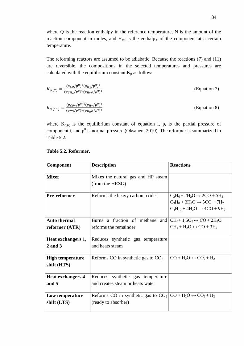
The reforming reactors are assumed to be adiabatic. Because the reactions (7) and (11)
are reversible, the compositions in the selected temperatures and pressures are
calculated with the equilibrium constant Kp as follows:
(Equation 7)
(Equation 8)
where Kp,(i) is the equilibrium constant of equation i, pi is the partial pressure of
component i, and p0 is normal pressure (Oksanen, 2010). The reformer is summarized in
Table 5.2.
Table 5.2. Reformer.
Component Description Reactions
Mixer Mixes the natural gas and HP steam
(from the HRSG)
Pre-reformer Reforms the heavy carbon oxides C2H6 + 2H2O → 2CO + 5H2
C3H8 + 3H2O → 3CO + 7H2
C4H10 + 4H2O → 4CO + 9H2
Auto thermal
reformer (ATR)
Burns a fraction of methane and
reforms the remainder
CH4+ 1,5O2 ↔ CO + 2H2O
CH4 + H2O ↔ CO + 3H2
Heat exchangers 1,
2 and 3
Reduces synthetic gas temperature
and heats steam
High temperature
shift (HTS)
Reforms CO in synthetic gas to CO2 CO + H2O ↔ CO2 + H2
Heat exchangers 4
and 5
Reduces synthetic gas temperature
and creates steam or heats water
Low temperature
shift (LTS)
Reforms CO in synthetic gas to CO2
(ready to absorber)
CO + H2O ↔ CO2 + H2

35
5.2.2 CO2 removal and compression
The main components of the CO2 removal and compression unit are the absorber tower,
the stripper tower, and the compressors. They are modeled using the Aspen Plus ®. The
process values in CO2 removal are chosen as in the literature (Corradetti and Desideri,
2005; NETL 2010; Kvamsdal et al, 2006; Bolland and Nord, 2011). The absorption
stripper model structure is based on the article by Corradetti and Desideri (2005) and a
report by NETL (2002). The equilibrium diagram for CO2 removal and compression
unit is presented in Figure 5.9. The absorption stripper process is presented in detail in
Figure 5.10.
Figure 5.9. CO2 removal and compression unit.
Figure 5.10. Absorption stripper process flow.
CO2 removal is accomplished by the MDEA and DEA absorption process. The MDEA
and DEA process is chosen because only A small amount of steam is required for
regeneration of the solvent in the stripper. The solvent used is a mix of MDEA, DEA
Absorber UnitSG SG
Solvents
CO2 LPS from
ST
Water to FWT
Absorber Stripper
Flash Heat Exchanger
CO2 compression
Solvent
mixer
Synthetic gas
CO2 rich solventCO2 lean
solvent
solvent
30% MDEA
5% DEA
65% water
CO2
CO2
CO2 lean
synthetic gas
36
and water. MDEA is chosen because of its low energy requirements, high capacity, and
stability in acid gas removal. MDEA is also less corrosive than other amines, thus
cheaper building material can be used. The disadvantage in using MDEA is its low rate
of reaction with CO2. The addition of DEA increases the rate of CO2 absorption
significantly without diminishing MDEA’s many advantages. (Kohl and Nielsen, 1997)
If it is assumed that equilibrium is attained in both the absorption and stripping steps
and isothermal conditions are maintained, the maximum net capacity of the CO2
removal unit is the difference between equilibrium concentrations at the absorption and
stripping partial pressures. Equilibrium reactions are presented below. Carbamate
formation does not happen to MDEA. (Kohl and Nielsen, 1997)
Equilibrium reactions:
Ionization of water:
H2O = H+ + OH
– (Reaction 12)
Hydrolysis and ionization of dissolved CO2:
CO2 + H2O = HCO3– + H
+ (Reaction 13)
Protonation of alkanolamine:
MDEA + H+ = MDEA
+ (Reaction 14)
DEA + H+ = DEA
+ (Reaction 15)
Carbamate formation:
DEA + HCO3–
= DEACOO– + H
+ (Reaction 16)
The amines and water are mixed in a mixer. The lean solvent, added MDEA, DEA and
water are conducted to the mixer. The solvent from the mixer is fed to the absorber
column from the upper part of the column. Synthetic gas is fed to the absorber tower
from the lower part of the column. Water is removed from the synthetic gas before
conducting it to the absorber column. The CO2-rich solvent is removed from the bottom
of the absorber column. Cleaned synthetic gas is removed from the top of the absorber
column.
CO2-rich solvent is then conducted to a flash drum, where the pressure is lowered. The
reduction in the pressure releases part of the CO2, which is conducted to compression.

37
The remainder of the CO2 is desorbed form the solvent in the stripper column. The
stripping agent is the vapor of the solvent itself, which is produced in a reboiler. The
steam, that evaporates the solvent in the reboiler, is extracted from the low pressure end
in the steam turbine.
From the stripper column, the lean solvent is conducted back to the mixer. Because of
the temperature difference between the lean solvent and the rich solvent, a heat
exchanger is placed after the lean solvent pump for lean solvent and before the stripper
for rich solvent. CO2 leaving the top of the stripper column is compressed and liquefied
to 7 bar and -50°C. The compressor unit available in the Aspen Plus ® could not liquefy
CO2. The liquefaction was done in a flash drum. The thermal power of the flash drum
was then converted into the work that should be done. The conversion was done by
using the coefficient of performance (COP) value 1.5 (Ramgen Power Systems, 2009).
5.3 Reference Plant
The results are compared to a conventional CCGT CHP without CO2 capture. The
reference plant is based on the same two gas turbines as the case with CO2 capture. It is
modeled with the Solvo ®. The heat production of the reference plant is fixed to be
roughly the same as in the cases with CO2 capture. The heat production of the CCGT
CHP without CO2 capture would otherwise be higher. The reduction of the heat
production results in a slightly higher power-to-heat ratio. Thus, a condensing unit of
steam turbine is needed for the steam to expand to lower pressure.
It is clear that all the effects of CO2 capture technology on the the CCGT CHP are due
to the changes in the power plant. The effects depend on how the added technology is
integrated into the CCGT CHP. In the case of the thesis, the rate of integration is high,
especially between the reformer and the HRSG. The main differences between the
conventional CCGT CHP and the CCGT CHP with pre-combustion CO2 capture
technology can be seen in Figures 5.11 and 5.12.

38
Figure 5.11. CCGT CHP with CO2 capture
Figure 5.12. CCGT CHP without CO2 capture.
As the figures above show, the main differences are the fuel entering the gas turbine,
integration between HRSG and the reformer, extraction from the steam turbine to the
reformer and to the absorber. The figures are simplified and only the main streams are
shown.
Gas Turbine HRSG Steam Turbine
Electricity
Exhaust
gases Steam
Synthetic gas
from
absorberElectricity
District heatingReformer Reformer Absorber
Gas Turbine HRSG Steam Turbine
Electricity
Exhaust
gases SteamNatural gasElectricity
District heating

39
6 COST ASSUMPTIONS
In this chapter the cost assumption of the power plant are presented. First, the operating
hours of the power plant are calculated. Then the total investment cost and the prices of
consumables and products are estimated. Taxes are included in the prices, except value
added tax (VAT).
6.1 Operating hours
The size of the power plant is approximated from the heat demand of the area where the
power plant is built. It is assumed that all the electricity that is produced along with the
heat can be sold on the power market. The size of the power plant is a major assumption
affecting the total costs of the plant.
The heat production in 2010 at the power plant site on which the power plant modeled
in this thesis is planned to be located is presented in Figure 6.1. The data, on the basis of
which the figure is drawn, is not completely reliable. Many errors, e.g. values below
zero, were found when the data was cleaned. The heat demand duration curve in the
area where the power plant is located is based on data from two years, and is presented
in Figure 6.2. The red area in the Figure 6.2 illustrates the main demand which the
power plant is planned to meet. Figure 6.1 is drawn on the basis of raw data and Figure
6.2 on the basis of cleaned data. (Fortum, 2011)
Figure 6.1. Heat production. (Based on Fortum, 2011)
0,0
100,0
200,0
300,0
400,0
500,0
600,0
700,0
Hea
t p
rod
uct
ion
(M
W)

40
Figure 6.2. Heat demand duration curve. (Based on Fortum, 2011)
The peak load can be defined as the power demand, the duration of which is less than
500 hours. The base load demand duration is at least 6,500 hours. (VTT, 2004) As seen
in Figure 6.2, the power plant designed here meets neither peak nor base load demand.
Thus, it is an intermediate load power plant. The power plant operates 4,776 hours per
year at full load, which are the peak operation hours.
It is assumed that the heat demand will not change dramatically in the future. This
assumption has to be made because the startup year for the power plant is 2020. The
startup year has been chosen to be as far in the future because the technology modeled
here is most likely to be in use then (Energy Policy for Europe, 2007).
6.2 Total Investment Cost
The costs of the power plant are mainly evaluated based on the literature. The
investment costs are presented in Table 6.1. The cost information found in the literature
is scaled to the case in the thesis based on reference scaling percentages in the VTT
publication (2004). Doubling the size of the power plant increases the investment cost
by 60% and decreases unit cost 20% (VTT, 2004). As mentioned in chapter 4, the
accuracy of the calculation method is between -30% and +50%. Even though reliable
cost information was found, it must be emphasized that the assumptions here are not
made directly from the power plant data. The assumptions are made based on the best
available information.
0
100
200
300
400
500
600
700
800
900
Hea
t d
eman
d (
MW
)
Time (h)

41
Table 6.1. Investment cost breakdown. (Foster Wheeler, 2010; Raiko, 2011)
TOTAL INVESTMENT COST M€
Power plant (2 GT+HRSG, ST, DH) 303
CO2 removal, compression and liquefaction 156
Reformer 508
Balance of plant 168
TOTAL 1,135
The investment cost of a Combined Cycle Gas Turbine (CCGT), based on the same gas
turbines without carbon capture, for power and heat production is expected to be €270
million (Raiko, 2011). The power plant unit cost with pre-combustion carbon capture is
estimated to be 1.12 times the conventional power plant cost (Foster Wheeler, 2011).
This is mainly due to the modifications that have to be made to the gas turbine for
hydrogen combustion.
The reformer investment cost is high compared to the other components. However, it
can be assumed that the reformer technology in power plant use is in an early stage in
the learning curve. The learning curve is based on a finding that the time needed to
produce a product shortens the more the product is produced (Haverila et al, 2005). It
can be used when setting the price for the product. For an example of the effect, the
impact of the learning curve on electricity production costs in wind power is presented
in Figure 6.3. Thus, it can be assumed that the cost of the reformer will decrease in the
future.

42
Figure 6.3. Wind power learning curve. (Wind Energy, 2011)
In calculations, an interest rate of 5% is used. The interest rate is chosen because it is
the usual interest rate used in Finland when comparing power sector investments (VTT,
2004).
6.3 Operating Cost and Revenue
Operating costs are divided into fixed and variable costs. Variable costs are estimated
based on the price forecast for natural gas, solvents, raw water and emission allowance.
The prices of the consumables are presented in Table 6.2. The prices of solvents are
based on the Foster Wheeler report (2010) and the ICIS report (2010). The prices of
transportation and storage of CO2 are based on the VTT report (2011).
The avarage price of natural gas in 2010 for a user similar to the power plant modeled
in the thesis was €31 / MWh (SVT, 2011). Kangas (2007) has forecast the price of
natural gas to be €35 / MWh in 2020 in Europe. The value of €31 / MWh has been
chosen. The price of natural gas depends, among other things, on the price of haevy fuel
oil. Thus, it is challenging to forecast future prices, and it is more reliable to use the
current prices.
Taxes on natural gas are now €9.024 / MWh. They include energy content tax, carbon
dioxide tax and maintenance support performance fee. The energy content tax is now €3

43
/MWh, but it is planned to be rised to €7.70 / MWh in 2015. However, the situation is
going to be evaluated before the later tax increase. (Tullihallitus, 2011)
Energy taxes must be paid on the fuel in heat production, but not on electricity
production. The amount of natural gas on which taxes must be paid is the amount of
heat produced multiplied by 0.9. (Tullihallitus, 2011)
Table 6.2. Variable operating cost break down.
Consumables Price
Natural gas €31 / MWh (taxes excluded)
€45 / MWh (taxes included)
MDEA €3,830 / tonne
DEA €1,000 / tonne
Raw water €0.102 / 1,000 l
CO2 transport €15 / CO2-tonne
CO2 storage €11 / CO2-tonne
As seen in the table above, emission allowances are not handled as variable costs here.
In this approach, emission allowances are regarded as consumables which have to be
bought from the market based on the polluting rate. It is deemed that CO2 cannot be
“produced” without a CO2 allowance. In other words, the CO2 allowance is the “raw
material” for CO2 emissions into the atmosphere.
However, it is assumed here that emission allowances are given to a company free of
charge. Thus, because they do not need all of them, they can sell them. In contrast to the
alternative approach presented above, here the emission allowances are “produced” by
capturing CO2. The cost of CO2 capture should be covered by selling emission
allowances. The differences in approaches is shown in Figure 6.4.

44
Figure 6.4. Approaches to emission allowance calculations.
By choosing the latter approach, the results do not have to be compared to the CCGT
CHP without CO2 capture. In the first approach, the feasibility of CO2 capture would
have been evaluated by comparing the costs of CCGT CHP with CO2 capture to CCGT
CHP without CO2 capture. In the latter approach, it is evaluated comparing the cost of
CO2 capture and the revenue from selling the emission allowances. The assumption that
all the emission allowances are granted free of charge for the CCGT CHP with CO2
capture is supported by the European Commission (2010) decision to support the CCS
project with emission allowances through the NER300 instrument.
Fixed operating costs are labor, maintenance and overhead costs. It is assumed that the
number of personnel required to operate the power plant is five for each of four shifts.
The labor costs in the electricity, heat, and gas sector in 2008 were €56,500 per person
(SVT, 2008).
Overhead costs are assumed to be 30% of the operating labor costs. The fixed costs are
presented in Table 6.3. Maintenance costs are estimated as 3% of the total investment
costs. (Foster Wheeler, 2010)
Without carbon capture With carbon capture
Captured
Sold allowances
Bought allowances
Emissions
Given allowances
Captured CO2

45
Table 6.3. Fixed operating costs.
Labor €56,500 / employee
Maintenance 3% of total investment costs
Overhead changes 30% of labor costs
Revenues are estimated based on the price forecast for electricity, heat and emission
allowances. The prices are shown in Table 6.4. The annual avarage of the Nord Pool
spot electricity price in 2010 in Finland was €56.64 / MWh (Nord Pool, 2011). The
price of electricity in the startup year of the power plant is forecast to be €100 / MWh
by Koskelainen (2010), and €47 / MWh by Pöyry Oy (Laatikainen, 2011). Because the
natural gas price was chosen to be the avarage price in 2010, the electricity price, too,
has been chosen to be the same as in 2010.
From 1 January 2011 to 1 August 2011 the price of the emission allowance forward to
the year 2015 has been between €15–25 / CO2-tonne (EEX, 2011). Koskelainen (2010)
forecast the emission allowance price to be €40 / CO2-tonne in 2020. In a bill (HE
152/2010 vp) on electricity production subsidy for renewable fuels, the emission
allowance price was estimated to be €20 / CO2-tonne in 2020. Reuters reported that
Barcap Capital lowered the average price forecast for the period 2013 to 2020 to €30 /
CO2-tonne from €40 / CO2-tonne. Reuters (2010) forecast the emission allowance price
to be €29.90 / CO2-tonne. Based on these forecasts, the emission allowance price €30 /
CO2-tonne has been chosen because it can be expected that the price of the emission
allowance will rise when the number of emission allowances on the market is reduced
(European Commission, 2010).
The price of district heating is based on the district heating prices in the area where the
power plant is planned to be located. The prices of district heating in Finland are
available from the internet pages of Energiateollisuus (Energiateollisuus, 2011).

46
Table 6.4. Prices of electricity, heat, and emission allowance.
Prices
Electricity €57 / MWh
Heat €55 / MWh
Emission allowance €30 / CO2-tonne
The total cash flow is presented in Figure 6.5. All prices are expected to increase at an
annual inflation rate of 2.5%.
Figure 6.5. Cash flow.
Natural gas supply
Heat and Power
Production
CO2 capture
CO2 conditioning
and compression
CO2 transportation
and storage
ElectricityDistrict
heating
€€
€
€
€
Solvents
€
Raw water
€
Emission allowance
€Work

47
7 PROCESS MODEL RESULTS AND
DISCUSSION
This chapter presents the results of the process modeling. The CCS case is compared to
the reference case.
The operation of the power plant was modeled with three different CO2 capture rates
(97%, 90%, and 80%). Also four different loads (100%, 90%, 80%, and 70%) were
modeled. However, the effects of the partial loads could not be reliably simulated
because the factors that should be fixed could not be in the Aspen and Excel models.
Thus, the partial load cases need further attention, and the results of the simulations are
not reported here.
As mentioned in chapter 1, the effects on following parameters were studied:
- energy efficiency
- power-to-heat ratio
- fuel input
- emissions
Simulation with the model was challenging, as it is composed of four separate models.
The large number of integrations between the models made it difficult to get the whole
model to converge.
7.1 Process Modeling
The summary of the plant performance at full load and with a capture rate of 90% is
presented in Table 7.1. The results of the reference plant are also included in the table.

48
Table 7.1. Plant performance.
PLANT THERMAL INPUT CCGT CHP with
CO2 capture
CCGT CHP without
CO2 capture
Thermal Energy of Natural Gas 1,003 MW 841 MW
PLANT ELECTRICAL OUTPUT
Electric Power Output at Generator
Gas Turbine 294 MW 273 MW
Steam Turbine 152 MW 130 MW
Total 446 MW 403 MW
Gross Electrical Efficiency 0.44 0.48
Auxiliary Electrical Consumption 21 MW 1,7 MW
Net Electrical Output 425 MW 401 MW
Net Electrical Efficiency 0.42 0.48
PLANT THERMAL OUTPUT
District Heating 353MW 351 MW
Absorber Unit Heat Consumption 96 MW -
OVERALL PLANT EFFICIENCY
0.78 0.89
POWER TO HEAT RATIO
1.20 1.14

49
7.1.1 Efficiency
As expected, the efficiency of the power plant is lower than the efficiency of a CCGT
without CO2 capture. The efficiency of a CCGT CHP without CO2 capture can be up to
91%. The drop in this case is 11% units.
In a previous study, the drop has been 21% units (Foster Wheeler, 2010). The difference
might be due to auxiliary electrical consumption that is much higher in the Foster
Wheeler (2010) study. This raises a question if all the auxiliaries are taken into account
in this case. Another possible reason is different process steam and water integration
between the HRSG unit and the reformer unit. In addition, it was assumed here that
there were no losses in the integration. One possible reason is different decisions made
in the tradeoff between CO2 removal heat consumption and the solvent leakage
situation. Also, a different CO2 condition at the calculation limit might be a reason for
the difference in the efficiency. If CO2 is to be transported in a pipeline, it is pressurized
to a higher pressure than in the case in the thesis in which the CO2 is liquefied for ship
transportation. However, none of these reasons are likely to cause the difference alone.
Thus, it can be concluded that the difference is a combination of more than a one cause.
In previous studies the efficiency drop for CCGT power production without heat
production has been 5–8% units (Kvamsdal & al. 2007; NETL, 2010). This means a
9%–15% drop in efficiency. Here, the total drop in total plant efficiency is 11%. The
drop in electrical efficiency is 6% units, which is 13% from the net electrical efficiency
of the CCGT CHP without CO2 capture. This falls into the same range as in the
previous studies of CO2 capture in a CCGT without heat production. It was expected
that the energy penalty for electricity production would be lower in CHP production
than in condensing power production because in CHP the energy penalty caused by the
CO2 capture is divided between power and heat production. However, the net electrical
efficiency is lower in CHP production than in CCGT power production. Thus, the
decrease of 1% unit is less in percentages in the condensing power case than in the CHP
case.
In the previous study the efficiency drop for coal-fired CHP was only 5% units.
However, the drop in electrical efficiency is 12% units. The lower total efficiency is due
to the increase in heat efficiency by 9% units. (Gode and Hagberg, 2008)
The CCGT CHP has better efficiency than the coal CHP. However, the CCGT CHP
with CO2 capture case in the thesis has lower efficiency than the Gode and Hagberg
(2008) coal CCS case in which it was 0.86. On the other hand, in the Gode and Hagberg
(2008) coal CCS case, the drop in electricity efficiency is greater than in the CO2
capture case in the thesis. Because the heat load is the factor that states the size of the
CHP plant, the CCGT CHP would produce significantly more electricity than coal-fired

50
CHP. The reasons behind the difference cannot be further examined because there was
not enough information about the coal case available.
7.1.2 Power-to-Heat Ratio
The power-to-heat ratio for a modern CCGT CHP is higher than 1.00. For example, the
power-to-heat ratio of the Suomenoja CCGT CHP is 1.09 (Fortum, 2010). In the
reference case, the power-to-heat ratio is 1.14. The relatively high power-to-heat ratio in
the reference case is due to the added condensing unit of the steam turbine, where part
of the steam is not extracted to district heating heat exchangers, thus it expands to the
condenser pressure, producing more electricity. This is done because the reference plant
is fixed to produce roughly the same amount of heat for being comparable to the CCS
case.
Another possible way to compare the results between the reference plant and the CCGT
CHP with CO2 capture is not to fix the heat production. In that case, the reference plant
would have a higher heat output, and thus have lower peak operation hours, as seen in
Figure 6.2, chapter 6.1.
In the CCGT CHP with CO2 capture, the power-to-heat ratio is 1.2. This is higher than
in the reference case. This indicates that the energy penalty of CO2 capture unit is higher
for heat than for electricity. This can be explained by the large steam extraction from the
steam turbine to the absorber in the CO2 removal unit. The extraction is carried out at
around the same pressures as the extractions to the district heating heat exchangers. This
reduces the steam mass flow to the district heating heat exchangers, but the steam
expands to the same pressure as in these extractions. This can be seen in Figure 7.1,
where the energy flows to the CCGT CHP with and without CO2 capture are presented.
The heat extraction to the absorber is larger than the heat consumption of the absorber
because not all the heat can be exchanged in the reboiler and in the absorber. The
extraction from the steam turbine to the reformer in the CO2 removal unit does not
affect the power-to-heat ratio as much because it is taken from a higher pressure and
thus affects both heat and electricity production.

51
Figure 7.1. The energy flows to the CCGT CHP with and without CO2 capture.
The CCGT CHP with CO2 capture produces more electricity in the steam turbine
because the mass flow in the steam turbine is larger than in the reference case. The mass
flow is larger because steam is produced in both the HRSG and the reformer. In the
reference case, steam is only produced in the HRSG.
7.1.3 CO2 Emissions
Annual CO2 emissions are 91 kt in the case of the 90% capture rate. Total CO2
emissions from the energy industry in Finland were 25 Mt in 2009 (SVT, 2011), which
does not include the emissions from industrial energy production. The reference plant
without CO2 capture produces 802 kt of CO2 annually. The avoided CO2 emissions in
this case would be 802–91 kt = 711 kt. This is presented in Figure 7.2.
Figure 7.2. Avoided CO2 emissions.
Gas Turbine HRSG Steam Turbine
Electricity
Exhaust
gases Steam
Synthetic gas
from
absorberElectricity
District heatingReformer Reformer Absorber
1003 MW
(W/O 841 MW NG)
152 MW
(W/O 130 MW)
294 MW
(W/O 273 MW)
353 MW
(W/O 351 MW)
68 MW 110 MWΔ 266 MW
0 200 400 600 800 1000
90%
0%
CO2 (kt/a)
Cap
ture
rat
e
Emissions into the atmosphere
Captured
Avoided CO2 Avoided CO2

52
According to a previous study, the ATR pre-combustion capture technology in a CCGT
has accomplished CO2 emissions of 42 kg/MWh in pure electricity production
(Kvamsdal et al, 2007).The CO2 emissions per electricity produced are shown in Figure
7.3.
Figure 7.3. CO2 emission per electricity produced.
7.2 Sensitivity Analysis
The different capture rate cases are simulated in such a way that in every case the gas
turbine operation is optimal. Thus, the electrical power output of the gas turbine is the
same in every case, even though the composition of the gas entering the gas turbine
changes. The compositions of these gases are shown in Table 7.2.
Because of the changed composition of the gas, the heating value is different, too. Thus,
the amount of gas needed to produce the same amount of electricity in the gas turbine is
higher when the capture rate is lower. However, the change in natural gas consumption
is minor. This is due to the amount of CO2 separated in the CO2 removal unit.
0
5
10
15
20
25
30
35
40
45
CCGT 90% Capture Rate
(Kvamsdal et al, 2007)
CCGT CHP 90% Capture
Rate
CO
2 E
mis
sions
(kg/M
Wh
elec
tric
ity)

53
Table 7.2. Synthetic gas entering the gas turbine.
Capture rate 97% 90% 80%
Gas composition
before gas turbine
(after CO2
separation) (mol-%)
H2 46.7 46.1 45.4
N2 46.0 45.2 44.4
CH4 6.8 6.8 6.7
CO2 0.5 1.9 3.5
SUM 100 100 100
7.2.1 Efficiency
As expected, overall plant efficiency is higher the lower is the capture rate. This is
shown in Figure 7.4. Although the electrical output of the gas turbine generator does not
change, the electrical output of the steam turbine generator does change. Moreover,
district heating power increases when the capture rate decreases.
The rate of change in efficiency increases when the capture rate increases. Efficiency
decreases by 0.12%-units from a capture rate of 80% to 90% when the capture rate
increases by 1% unit. Efficiency decreases by 0.19 % units from a capture rate of 90%
to 97% when the capture rate increases by 1% unit. Thus, the more CO2 captured, the
more fuel is needed to produce the same amount of heat and electricity.

54
Figure 7.4. Overall Plant Efficiency.
7.2.2 Power to Heat Ratio
The change in electricity output from the steam turbine is due to the change in the
reboiler duty in the CO2 separation unit. The steam conducted to the reboiler is
extracted from the steam turbine at different pressures, depending on the capture rate.
The mass flow of the steam extracted from the steam turbine is larger the higher the
capture rate is. The change in capture rate affects almost equally heat production and
electricity production. This is shown in Figure 7.5.
The effect of the change in capture rate is equal in both heat and electricity production
because of the change in mass flows. The extraction to the absorber unit is larger the
higher the capture rate is. This should reduce more heat production than electricity
production because the steam extraction to the absorber unit is at the same pressure as
the extraction to the district heating heat exchangers. The electricity production of the
gas turbine is the same in every capture rate case. The mass flow of fuel entering the gas
turbine changes because the heating value of the synthetic gas entering the gas turbine
changes. Thus, the natural gas input changes; more heat is produced in the reformer and
more steam enters the steam turbine. This is shown in Table 7.3.
0,70
0,71
0,72
0,73
0,74
0,75
0,76
0,77
0,78
0,79
0,80
97% 90% 80%
Over
all
Pla
nt
Eff
icie
ncy
Capture Rate
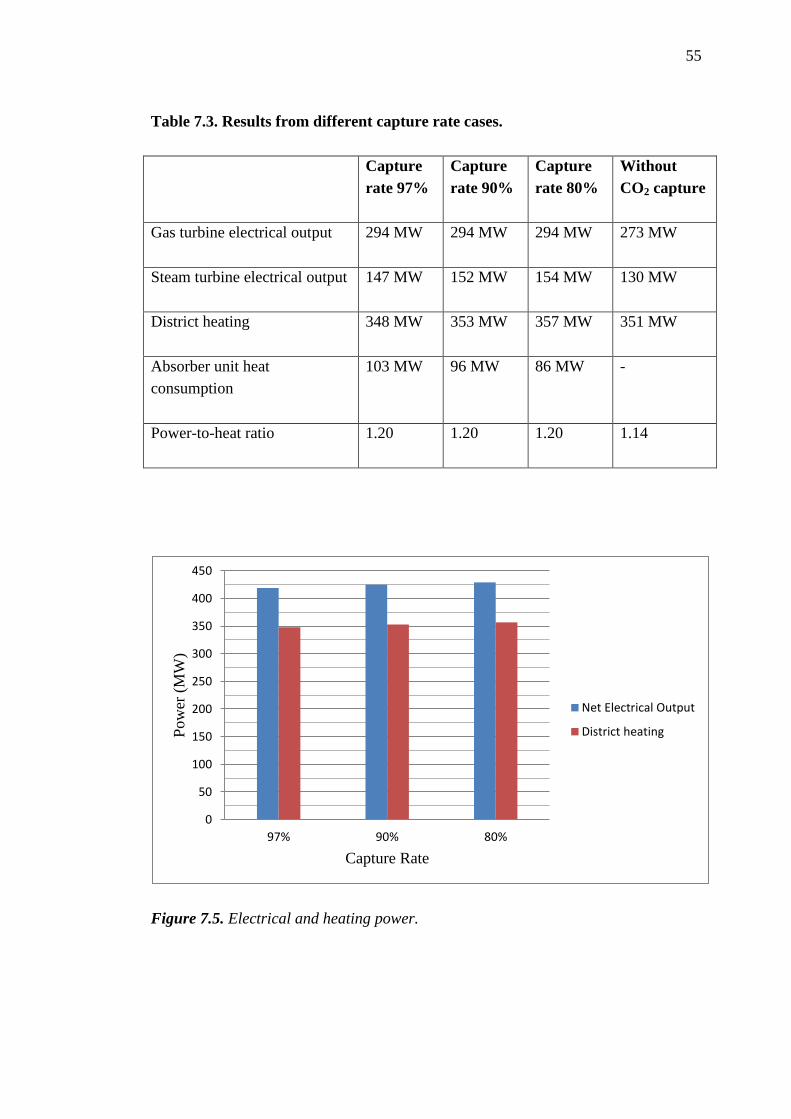
55
Table 7.3. Results from different capture rate cases.
Capture
rate 97%
Capture
rate 90%
Capture
rate 80%
Without
CO2 capture
Gas turbine electrical output 294 MW 294 MW 294 MW 273 MW
Steam turbine electrical output 147 MW 152 MW 154 MW 130 MW
District heating 348 MW 353 MW 357 MW 351 MW
Absorber unit heat
consumption
103 MW 96 MW 86 MW -
Power-to-heat ratio 1.20 1.20 1.20 1.14
Figure 7.5. Electrical and heating power.
0
50
100
150
200
250
300
350
400
450
97% 90% 80%
Pow
er (
MW
)
Capture Rate
Net Electrical Output
District heating

56
7.2.3 CO2 Emissions and fuel input
Because the natural gas input changes only slightly when the capture rate changes, the
change in the amount of the CO2 captured is the same as the change in the amount of the
CO2 emissions into the atmosphere. This is shown in Figure 7.6.
Figure 7.6. CO2 emissions with different capture rates.
This is expected because of the choices made in modeling. The gas turbine produces the
same amount of electricity in all of the cases. Thus, it demands roughly the same
amount of fuel. Not exactly the same because of the slight change in the composition of
the synthetic gas entering the gas turbine. However, it can be concluded from these
results that natural gas consumption will grow if the capture rate is increased and the
heat production is fixed. This is shown in Figure 7.7, in which the natural gas input is
divided by the heat production. Also, the natural gas input is divided by the electricity
production in the same figure. In both cases, all the natural gas input is allocated for the
other, heat or electricity.
0 200 400 600 800 1000
97%
90%
80%
CO2 (kt/a)
Cap
ture
Rat
e
Actual
Captured

57
Figure 7.7. Natural gas input.
The CO2 emissions per heat or electricity produced are presented in Figure 7.8. As seen
in the figure, the reduction in the CO2 emission per electricity and heat produced seems
linear in the function of capture rate.
Figure 7.8. CO2 emissions per heat and electricity produced.
160
165
170
175
180
185
190
195
200
205
210
80% 85% 90% 95%
Nat
ura
l gas
input
(kg/M
Wh)
Capture rate
Input per Heat Produced
Input per ElectricityProduced
0
20
40
60
80
100
120
80% 85% 90% 95%
CO
2 E
mis
sions
(kg/M
Wh)
Capture rate
Emissions per HeatProduced
Emissions per ElectricityProduced

58
However, the change is only almost linear. The rate of change from a capture rate of
80% to 90% is 5.42 kg/MWhheat and 4.52 kg/MWhelectricity per 1% change in capture
rate. From 90% to 97% the rate of change is higher, 5.66 kg/MWhheat and 4.70
kg/MWhelectricity per 1% change in capture rate. Even though the change is so small that
it cannot be seen in the figure, it is important because it was noticed previously in this
study that efficiency does not change linearly when capture rate changes. Also the
natural gas input changed only slightly. Thus, the CO2 emissions per heat or electricity
produced cannot change linearly when capture rate changes.
7.3 Further discussion
The results in the thesis represent only the effects of one possible pre-combustion
integration into a new CCGT CHP power plant. Other integrations might cause very
different kinds of results. This becomes especially important when the efficiency and
power-to-heat ratio parameters are compared.
This is shown when the study of coal CHP CCS case is compared to the case in the
thesis. In the coal CHP case, the heat production increased while the total efficiency
decreased (Gode and Hagberg, 2008). Thus, the power-to-heat ratio decreased. Here, the
power-to-heat ratio increased, while the efficiency decreased significantly. This begs the
question of whether it is possible to integrate CO2 capture into the CCGT CHP in such a
way that it would increase the heat production.
It is also possible that efficiency can be improved by different reformer or CO2
separation technology. Here, the reformer used is an ATR, which burns a fraction CH4
to provide heat to the system. It might be cheaper to bring the heat into the system from
outside. It would also be interesting to investigate whether heat for the CO2 separation
unit could be produced in a way that is cheaper than extracting it from the steam
turbine.
In the thesis, the CO2 capture rate is changed by changing the reboiler duty in the CO2
separation unit. There are also alternative separation rate changing options. For
example, it is possible that not all CH4 reforms into CO2 and H2O in the reformer. If
CH4 is conducted to the gas turbine and combusted, it increases the amount of CO2
emissions. The capture rate of the CO2 separation unit would not be the separation rate
of the whole system. This might have an effect on the total plant efficiency.
The biggest flaw of the model lies in the assumptions made in the gas turbine operation.
Even though it is possible to convert the gas turbine used in the thesis to hydrogen
combustion, it is not possible to model this conversion in the scope of this thesis.
However, this should not have caused a major inconsistency in the model because the
gas turbine unit modeled was able to combust hydrogen.

59
Another gas turbine parameter that could not be taken into account are NOX emissions.
The temperatures in hydrogen combustion might rise so high that thermal NOX starts
forming. The thermal NOX formation cannot be calculated, it should be measured. The
NOX emission could be evaluated from the burner information. Because it was assumed
that the gas turbine would burn hydrogen, the burners were not given attention. Thus, it
is not possible to evaluate NOX emissions in this thesis.
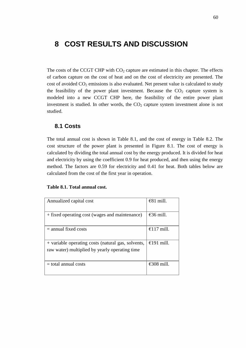
60
8 COST RESULTS AND DISCUSSION
The costs of the CCGT CHP with CO2 capture are estimated in this chapter. The effects
of carbon capture on the cost of heat and on the cost of electricity are presented. The
cost of avoided CO2 emissions is also evaluated. Net present value is calculated to study
the feasibility of the power plant investment. Because the CO2 capture system is
modeled into a new CCGT CHP here, the feasibility of the entire power plant
investment is studied. In other words, the CO2 capture system investment alone is not
studied.
8.1 Costs
The total annual cost is shown in Table 8.1, and the cost of energy in Table 8.2. The
cost structure of the power plant is presented in Figure 8.1. The cost of energy is
calculated by dividing the total annual cost by the energy produced. It is divided for heat
and electricity by using the coefficient 0.9 for heat produced, and then using the energy
method. The factors are 0.59 for electricity and 0.41 for heat. Both tables below are
calculated from the cost of the first year in operation.
Table 8.1. Total annual cost.
Annualized capital cost €81 mill.
+ fixed operating cost (wages and maintenance) €36 mill.
= annual fixed costs €117 mill.
+ variable operating costs (natural gas, solvents,
raw water) multiplied by yearly operating time
€191 mill.
= total annual costs €308 mill.

61
Table 8.2. Cost of energy.
Parameter Cost (€ / MWh)
Cost of energy 82
Cost of electricity 90
Cost of heat 75
The cost allocation between heat and electricity is a complicated issue, as mentioned in
chapter 4.1. The energy method used here takes into account the fact that the power-to-
heat ratio is higher in the case of the CCGT CHP with CO2 capture than in the case
without CO2 capture. Thus, more costs are allocated for electricity.
Figure 8.1. Cost structure.
As seen in the cost structure figure above, most of the power plant cost comes from the
fuel. The price of natural gas strongly affects the costs of the power plant. For
comparison, the cost structure of the reference plant is presented in Figure 8.2.
Annuity
Fixed operating costs
Natural gas
Other variable costs
Total €308 million
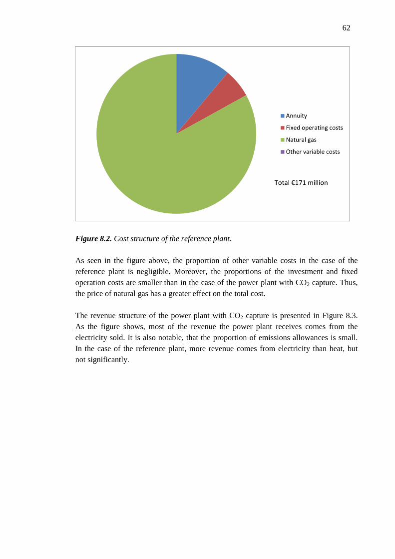
62
Figure 8.2. Cost structure of the reference plant.
As seen in the figure above, the proportion of other variable costs in the case of the
reference plant is negligible. Moreover, the proportions of the investment and fixed
operation costs are smaller than in the case of the power plant with CO2 capture. Thus,
the price of natural gas has a greater effect on the total cost.
The revenue structure of the power plant with CO2 capture is presented in Figure 8.3.
As the figure shows, most of the revenue the power plant receives comes from the
electricity sold. It is also notable, that the proportion of emissions allowances is small.
In the case of the reference plant, more revenue comes from electricity than heat, but
not significantly.
Annuity
Fixed operating costs
Natural gas
Other variable costs
Total €171 million

63
Figure 8.3. Revenue structure.
The power plant modeled here has relatively low operating hours. The effect of change
in operating hours on the cost of energy is shown in Figure 8.4. As seen in the figure
below, when the operating hours increase by 100 h, the cost of energy decreases by
€0.60 / MWh.
Figure 8.4. The effect of operating hours on the cost of energy.
Electricity
District heating
Emission allowances
Total €235 million
72
74
76
78
80
82
84
86
4500 4700 4900 5100 5300 5500 5700 5900 6100 6300 6500
Cost
of
Ener
gy (
€/M
Wh)
Operating hours per year (h)

64
The cost of avoided CO2 emission is shown in Table 8.3.
Table 8.3. Cost of avoided CO2 emissions.
Total annual costs €308 million
– Total annual costs in reference plant €171 million
Difference in total annual costs €137 million
/ The amount of avoided CO2 emissions 711 kt CO2
Cost of avoided CO2 emissions €193/CO2-tonne
Compared to previous studies, the cost is extremely high. For example, in the VTT
report (2011), the cost of avoided CO2 emissions in a milled peat-fuelled CHP plant is
€85/CO2-tonne. The power plant in the VTT study is smaller, which might suggest that
the investment costs are lower. The different results might also be due to different
calculation methods when calculating the cost of the power plant without CO2 capture.
When the CO2 removal unit was modeled, it was noticed that there was a tradeoff
between CO2 removal heat consumption and solvent leakage. The higher the heat
consumption, the lower the leakage is. Here, the CO2 removal unit is modeled on the
basis of an article by Corradetti and Desideri (2005), which gave an approximation for
the heat demand. Thus, the leakage did not receive much attention. This might cause
high solvent usage and therefore high solvent costs. It is not possible in the scope of this
thesis to investigate the tradeoff further.
The cases where most of the leakage solvent is recycled and where none of the leakage
solvent is recycled were modeled. However, the possible energy consumption of the
recycling was not taken into account. The effect of changed amount of solvent on total
annual cost in the first year of operation is shown in Figure 8.5. Linearity is assumed
because the energy consumption and other possible influences of the solvent leakage
recycling are not taken into account.

65
Figure 8.5. The relationship between total annual cost in the first year of operation and
the amount of added solvent.
As seen in Figure 8.5, if none of the solvent is recycled, the total annual cost increases
by 8.8% when compared to the situation where almost of all the solvent is recycled.
Compared to previous studies, the lower amount of added solvent seems more likely. In
the Foster Wheeler report (2010), the amount of added solvent is less than the lowest
case studied here. However, in the Foster Wheeler report (2010) the efficiency is lower.
This again indicates the significance of the tradeoff mentioned in the previous chapter.
Even though the recycling of the solvent is not taken into account in the process model
results, it is taken into account here. This can be done because it can be assumed that
almost all solvent leakage can be recycled without major changes in the process and
with minor energy consumption (NETL, 2002). Thus, further on it is assumed that
almost all the solvent can be recycled, and the amount of solvent leakage is 302 tonnes
per year, which is equal to 91 tonnes per year MDEA and 15 tonnes per year DEA. This
is based on the solvent stream calculations in the CO2 capture model.
8.2 Feasibility of the Investment
The present value of the power plant is calculated with three different interest rates 5%,
7%, and 10%. In all cases the net present value is negative. Thus, the power plant
investment is not feasible in the assumed scenario.
300
305
310
315
320
325
330
335
0 2000 4000 6000 8000 10000 12000 14000 16000 18000
Tota
l A
nn
ual
Cost
(M
€)
Added solvent (MDEA 30%, DEA 5%) (t/a)

66
Besides the price of reformer, the factors that affect the feasibility of the the investment
the most are the prices of electricity, heat, emission allowance and natural gas. The
boundary values for these factors are presented in Table 8.4. The boundary value here is
the value when the net present value is zero. In other words, if the value of the factor is
more than the boundary value, the investment becomes feasible. Except in the case of
natural gas, where the value should be lower to make the investment feasible.
Table 8.4. Boundary values.
Factor Boundary Price
Electricity €85 / MWh
District Heating €88 / MWh
Emission Allowance €96 / CO2-tonne
Natural Gas €19 / MWh
As seen in the table above, the boundaries are high for electricity, district heating and
emission allowance prices. The boundary price for natural gas is low. However, there is
a strong relationship between the prices of electricity and emission allowances in the
Nordic market and it cannot be assumed that just one of them would change without the
other changing.
The boundary price of emission allowance is much lower than the price of avoided CO2
emissions, €193 / MWh. This is because the cost of a CCGT CHP without CO2 capture
affects the cost of avoided CO2 emissions, but not directly the feasibility of the CCGT
CHP with CO2 capture. The feasibility is calculated with the net present value, and the
cost of avoided CO2 emissions from the differences between the CCGT CHP with and
without CO2 capture. Also, the amount of avoided CO2 emissions is less than the
amount of CO2 captured, which is here assumed to be the number of CO2 emission
allowances sold.
It is reasonable to compare how changes in more than one component affect the
feasibility. The boundary price of natural gas as a function of the price of the emission
allowance is presented in Figure 8.6. The figure is calculated by keeping the net present
value as zero and changing the price of the emission allowance.

67
Figure 8.6. The price of natural gas as a function of the price of emission allowances
when the net present value is zero.
The price of natural gas was between €27/MWh and €43/MWh from January 2010 to
May 2011 (SVT, 2011). The increased tax rate has increased the price of natural gas
from the beginning of 2011 (SVT, 2011). As seen in the figure above, the natural gas
price of €32 / MWh yields an emission allowance price of €100 / CO2-tonne to make the
power plant investment feasible. This is an extremely high value. Currently, the
emission allowance price is €11 / CO2-tonne (EEX, 3 August 2011). Even though the
emission allowance price is expected to increase, the price of natural gas should
decrease, too, to make the investment feasible.
The boundary price of electricity as a function of the price of natural gas is presented in
Figure 8.7. The net present value is kept as zero.
5
10
15
20
25
30
35
40
0 50 100
Pri
ce o
f N
atura
l G
as w
ihto
ut
tax
es
(€/M
Wh)
Price of Emission Allowance (€/CO2-tonne)
Interest rate 5 %, NPV = 0
Interest rate 7 %, NPV = 0
Interest rate 10 %, NPV = 0

68
Figure 8.7. The price of electricity as a function of the price of natural gas when the net
present value is zero.
As seen in the figure above, the price of natural gas strongly affects the boundary price
of electricity. This is not surprising, as natural gas is the largest operating cost. When
the price of natural gas changes by €1 / MWh, the price of electricity changes by €2.3 /
MWh. This higher rate of change in the price of electricity is due to the efficiency of the
power plant. The efficiency of the power plant also affects the price of district heating.
The price of natural gas as a function of the price of district heating is shown in Figure
8.8.
40
50
60
70
80
90
100
110
120
130
140
20 25 30 35 40 45 50
Pri
ce o
f E
lect
rici
ty (
€/M
Wh)
Price of Natural Gas (€/MWh)
Interest rate 5 %, NPV = 0

69
Figure 8.8. The price of natural gas as a function of the price of heat when the net
present value is zero.
The price of electricity as a function of the price of emission allowance is presented in
Figure 8.9. As seen in the figure, the higher the price of emission allowances, the lower
the price of electricity needed for the investment to be feasible.
Figure 8.9. The price of electricity as a function of the price of emission allowances
when the net present value is zero.
55
65
75
85
95
105
115
125
135
145
20 25 30 35 40 45 50
Pri
ce o
f D
istr
ict
Hea
ting (
€/M
Wh)
Price of Natural Gas (€/MWh)
Interest rate 5 %, NPV = 0
40
50
60
70
80
90
100
0 20 40 60 80 100 120
Pri
ce o
f E
lect
rici
ty (
€/M
Wh)
Price of Emission Allowance (€/CO2-tonne)
Interest rate 5 %, NPV = 0
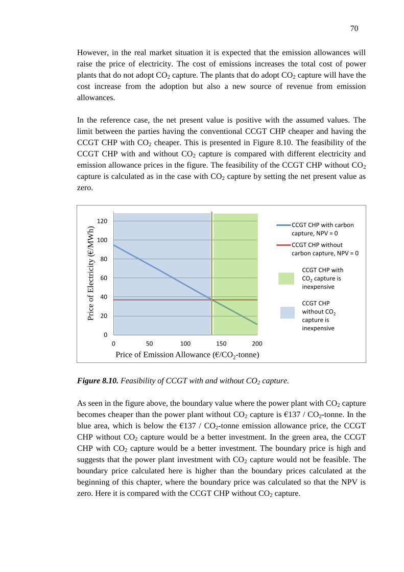
70
However, in the real market situation it is expected that the emission allowances will
raise the price of electricity. The cost of emissions increases the total cost of power
plants that do not adopt CO2 capture. The plants that do adopt CO2 capture will have the
cost increase from the adoption but also a new source of revenue from emission
allowances.
In the reference case, the net present value is positive with the assumed values. The
limit between the parties having the conventional CCGT CHP cheaper and having the
CCGT CHP with CO2 cheaper. This is presented in Figure 8.10. The feasibility of the
CCGT CHP with and without CO2 capture is compared with different electricity and
emission allowance prices in the figure. The feasibility of the CCGT CHP without CO2
capture is calculated as in the case with CO2 capture by setting the net present value as
zero.
Figure 8.10. Feasibility of CCGT with and without CO2 capture.
As seen in the figure above, the boundary value where the power plant with CO2 capture
becomes cheaper than the power plant without CO2 capture is €137 / CO2-tonne. In the
blue area, which is below the €137 / CO2-tonne emission allowance price, the CCGT
CHP without CO2 capture would be a better investment. In the green area, the CCGT
CHP with CO2 capture would be a better investment. The boundary price is high and
suggests that the power plant investment with CO2 capture would not be feasible. The
boundary price calculated here is higher than the boundary prices calculated at the
beginning of this chapter, where the boundary price was calculated so that the NPV is
zero. Here it is compared with the CCGT CHP without CO2 capture.
0
20
40
60
80
100
120
0 50 100 150 200
Pri
ce o
f E
lect
rici
ty (
€/M
Wh)
Price of Emission Allowance (€/CO2-tonne)
CCGT CHP with carboncapture, NPV = 0
CCGT CHP withoutcarbon capture, NPV = 0
CCGT CHP with CO2 capture is inexpensive
CCGT CHP without CO2 capture is inexpensive

71
The cost of CO2 emissions is analyzed in three different ways in the thesis. The results
are summarized in Table 8.5.
Table 8.5. The boundary prices for emission allowances.
Boundary price € / CO2-tonne
Cost of avoided CO2 emissions 193
Emission allowance when the NPV of CCGT
CHP with CO2 capture equals zero
96
Emission allowance when the NPV of CCGT
CHP with and without CO2 capture equals zero
137
The differences are due to different calculation methods. In the cost of avoided CO2
emissions only the avoided emissions are taken into account, and the costs that are
divided by the amount of emissions constitute the difference between the total annual
costs of the CCGT CHP with and without CO2 capture. In the second case in the table
above, only the costs of the CCGT CHP with CO2 capture are taken into account, and
the price of emission allowances are calculated by setting the NPV as zero. In the third
case in the table, the price of emission allowance is calculated by setting the NPV of the
CCGT CHP with and without CO2 capture as zero.
8.3 Further discussion
As mentioned in the cost assumptions in chapter 6, the cost of the power plant is not
calculated from the component prices, as such information was not directly available.
However, reliable cost information that had to be scaled was found. This might be a
source of error in the cost calculations.
Another possible error source in the feasibility calculations is the reliability of the
market information. The price information found for the emission allowance was hardly
high enough to cover the cost information found for the transportation and storage.
Thus, it cannot cover all the costs caused by CCS, which also include the costs of CO2
capture. This requires further market analysis to see how the prices can develop. Here, it
was also assumed that all captured CO2 could be sold as emission allowances. This
would most likely not be the case, and it would also affect the relationship of the cost of
transportation and storage and the price of emission allowances on the market.

72
9 SUMMARY AND CONCLUSIONS
The research question was: how does carbon capture affect a new gas turbine combined
cycle power plant with combined heat and power production? The effects on total plant
efficiency, electricity production efficiency, power-to-heat ratio, fuel input, CO2
emissions, CO2 avoidance cost and cost of electricity and heat production, especially,
were studied, and a sensitivity analysis was made.
Different CO2 capture technologies were briefly compared in the thesis. Based on the
comparison, a pre-combustion technology was chosen to be modeled. The technology
was modeled in a greenfield CCGT CHP power plant. The model was built with the
Solvo ®, MS Excel ®, and the AspenPlus ®.
The power plant was planned to be located on the coast of Finland. Heat demand in the
area of the site was the basis for the size of the power plant. The plant modeled
produces 353 MW of heat. Many assumptions had to be made when building the model,
especially in the cost evaluation.
The power plant modeled in the thesis is not feasible. The costs are high, and to cover
the costs of CO2 capture the emission allowance prices should be extremely high. It is
concluded that CCGT CHP with pre-combustion technology would not be a reasonable
investment with the current prices of electricity, heat, and emission allowances. The
main strengths of the plant were low rate of emissions and increased power-to-heat
ratio. The main weaknesses were high investment costs and decreased efficiency. The
results here are not completely in line with previous studies.
The thermodynamic results are fairly well in line with the previous studies. The
efficiency of the plant is lower than in the reference case. Compared with previous
studies, the amount of the decrease was surprisingly high. There are only a few previous
studies on CHP plants and, consequently, there were no expectations regarding the
power-to-heat ratio. The power-to-heat ratio increased slightly. Thus, the decrease in
efficiency affects heat production more than electricity production.
The cost results differ greatly from the previous studies. The cost of avoided CO2
emissions here is approximately twice as high as in the previous studies. The main
parameters affecting the cost of avoided CO2 emissions were the high investment cost
and low price of emission allowances.

73
In the thesis, the entire power plant was modeled and it has been found that all the
components require further attention. In particular, the integration between the reformer
and the HRSG, and the absorber with the rest of the process requires further attention.
The cost results are based on simple assumptions, which might not be feasible. A
complete market analysis might give more accurate price information and change the
results.

74
REFERENCES
2Co Energy. 2011. Don Valley Power Project. Available from
http://www.2coenergy.com/dv_project_description.html. Accessed on 2.8.2011.
AACE, American Association of Cost Engineers. 2011. Available from
http://www.aacei.org/mbr/whatIsCE.shtml. Accessed on 22.2.2011.
Aspen Tech. 2011. Available from http://www.aspentech.com/products/aspen-
plus.aspx. Accessed on 27.4.2011.
Bill. 2010. Hallituksen esitys Eduskunnalle laiksi uusiutuvilla energialähteillä tuotetun
sähkön tuotantotuesta. HE 152/2010 vp. Available from
http://www.finlex.fi/fi/esitykset/he/2010/20100152.pdf. Accessed on 3.8.2011.
Bolland, Olav; Nord, Lars. 2011. HRSG Design for Integrated Reforming Combined
Cycle With CO2 Capture. Journal of Engineering for Gas Turbines and Power.
Vol. 133.
Corradetti, Alessandro; Desideri, Umberto. 2005. Analysis of Gas-Steam Combined
Cycles With Natural Gas Reforming and CO2 Capture. Journal of Engineering
for Gas Turbines and Power. Vol. 127. pp.545-552.
Damen, Kay; van Troost, Martijn; Faaij, André, Turgenburg, Wim. 2006. A comparison
of electricity and hydrogen production system with CO2 capture and storage.
Part A: Review and selection of promising conversion and capture technologies.
Progress in Energy and Combustion Science. Vol. 32. pp.215-246.
EEX, European Energy Exchange. 2011. Emissions rights. Available from
http://www.eex.com/en/Market%20Data/Trading%20Data/Emission%20Rights.
Accessed on 22.7.2011.
Energiateollisuus. 2011. District heating prices. Available from
http://www.energia.fi/fi/tilastot/kaukolampotilastot/kaukolammonhinta.
Accessed on 3.8.2011.

75
Energy Policy for Europe. 2007. Available from http://eur-
lex.europa.eu/Notice.do?mode=dbl&lang=en&ihmlang=en&lng1=en,fi&lng2=c
s,da,de,el,en,es,et,fi,fr,hu,it,lt,lv,mt,nl,pl,pt,sk,sl,sv,&val=441123:cs&page.
Accessed on 10.8.2011.
EU, European Commission. 2011. Seventh Framework. Available from
http://cordis.europa.eu/fetch?CALLER=FP7_PROJ_EN&QZ_WEBSRCH=carb
on+capture&USR_SORT=EN_QVD+CHAR+DESC. Accessed on 18.2.2011.
EU, European Commission. 2010. Energy 2020 A strategy for competitive, sustainable
and secure energy. Comminication from the Commission to the Europen
Parliament, the Council, the Europen Economis and Social Committee and the
Committee of the Regions. Brussels. Europen Commission.
European Commission. 2010. Emissions Trading System (EU ETS). Available from
http://ec.europa.eu/clima/policies/ets/index_en.htm. Accessed on 3.8.2011.
European Commission. 2010. Decision. Official Journal of the European Union.
2010/670/EU. Available from http://eur-
lex.europa.eu/LexUriServ/LexUriServ.do?uri=OJ:L:2010:290:0039:0048:en:PD
F. Accessed on 9.8.2011.
EU. 2009. Directive 2009/31/EC of the European Parliament and of the Council.
Official Journal of the European Union. pp. L140/116-L140/117, L140/123.
European Commission. 2007. Directive 2009/31/EY. Hiilidioksidin geologinen
varastointi. Euroopan Unionin virallinen lehti. Available from http://eur-
lex.europa.eu/LexUriServ/LexUriServ.do?uri=OJ:L:2009:140:0114:0135:FI:PD
F. Accessed on 10.8.2011.
Fortum Oy. 2011. Solvo ®. Available from http://solvo.fi/index_en.shtm. Accessed on
27.4.2011.
Fortum Oy. 2011. Heat consumption data. Received 14.3.2011.
Fortum Oy. 2010. Fortum to discontinue Meri-Pori carbon capture and storage project.
Available from http://www.fortum.com/en/mediaroom/pages/fortum-to-
discontinue-meri-pori-carbon-capture-and-storage-project.aspx. Accessed on
2.8.2011.
Fortum Power and Heat Oy. 2010. Energiaa Suomenojan voimalaitokselta. [brochure]
Visited 27.1.2011.

76
Foster Wheeler Ltd., Fortum Oy. 2010. Assessment of Natural Gas Fuelled Power
Plants with Carbon Capture. [Confidential Report]
Fourier, Josep. 1836. General Remarks on the Temperature of the Terrestrial Globe and
the Planetary Spaces. Translated from French by Mr. Ebenezer Burges of
Ambers College. The American Journal of Science. Vol. 32. No. 1.
Gasum Oy. 2011. Natural Gas Composition. Available from
https://online.gasum.fi/online/yleisettiedot/Sivut/Maakaasun_koostumus.aspx.
Accessed on 28.6.2011.
Global CCS Intitute. 2011. Available from
http://www.globalccsinstitute.com/resources/projects/map. Accessed on
18.2.2011.
Gode, J.; Hagberg, L.. 2008. Systemanalys av CCS vid kraft värme. Available from
http://www.ivl.se/download/18.7df4c4e812d2da6a416800072060/B1870.pdf.
Accessed on 18.7.2011.
Haverila, Matti; Uusi-Rauva, Erkki; Kouri, Ilkka; Miettinen, Asko. 2005.
Teollisuustalous. 5th
edition. Tammerpaino Oy.
Horlock, J.H.. 1992. Combined Power Plants Including Combined Cycle Gas Turbine
(CCGT) Plants. Pergamon Press Ltd.
ICIS. 2010. Available from
http://www.icispricing.com/il_shared/Samples/SubPage10100082.asp. Accessed
on 1.7.2011.
ICIS. 2008. Available from
http://www.icis.com/Articles/2008/06/16/9132093/diethanolamine-prices-
rocket-on-demand-from-china-and-for-biofuels.html. Accessed on 1.7.2011.
IEA, International Energy Agency. 2008. Carbon Capture and Storage A key carbon
abatement option. Paris. IEA Publications. pp. 47-53.
IEA, International Energy Agency, 2010. Energy Technology Perspectives 2010
Scenarios & Strategies to 2050. Paris. IEA Publications. p.47, p.120.
IEA graphs, International Energy agency. 2010. Energy Technology Perspectives 2010,
Key Graphs. Available from http://iea.org/techno/etp/etp10/key_figures.pdf.
Accessed on 26.1.2011.

77
IFRF; Raiko, Risto; Saastamoinen, Jaakko; Hupa, Mikko; Kurki-Suonio, Ilmari. 2002.
Poltto ja palaminen. Gummerus Kirjapaino. p. 24.
IPCC, International Panel of Climate Change. 2005. Carbon Capture and Storage. USA.
Cambridge University Press. p.118.
Johnston, Lucy; Hausman, Ezra; Biewald, Bruce; Wilson, Rachel; White, David. 2011.
2011 Carbon Dioxide Price Forecast. Synapse Energy Economics Inc.Available
from http://www.synapse-energy.com/Downloads/SynapsePaper.2011-
02.0.2011-Carbon-Paper.A0029.pdf. Accessed on 3.8.2011.
Jonshagen, Klas; Sipöcz, Nikolett; Genrup, Magnus. 2011. A novel Approach of
Retrofitting a Combined Cycle With Post Combustion CO2 Capture. Journal of
Engineering for Gas Turbines and Power. Vol. 133.
Kangas, Hanna-Liisa. 2007. Euroopan Unionin maakaasumarkkinoiden kehitys vuoteen
2030: maakaasumarkkinamalli. Pro Gradu. University of Helsinki. Available
from http://www.helsinki.fi/taloustiede/tutkimus/ye/graduhannakangas.pdf.
Accessed on 3.8.2011.
Kaplan, Stan. 2008. Congressional Research Service Report for Congress. Power
Plants: Characteristics and Costs. Available from
http://www.fas.org/sgp/crs/misc/RL34746.pdf. Accessed on 23.2.2011.
Kehlhofer, Rolf H.; Warner, Judy; Nielsen, Henrik; Bachmann, Rolf. 1999. Combined-
Cycle Gas & Steam Turbine Power Plants. 2nd
Edition. PennWell Publishing
Company.
Kohl, Arthur; Nielsen, Richard. 1997. Gas Purification. 5th
Edition. Gulf Publishing
Company.
Koskelainen, Antti. 2010. Euroopan sähkömarkkinaintegraatio. Suomen ElFi Oy.
Available from
http://www.fingrid.fi/attachments/fi/media/Seminaarit/sm2010/elfi_koskelainen.
pdf. Accessed on 9.8.2011.
Kvamsdal, Hanne M.; Jordal, Kristin; Bolland, Olav. 2006. A Quantitative Comparison
of gas turbine cycles with CO2 capture. Energy. Vol. 32. Issue 1. pp. 10-24.
Laatikainen, Tuula. 2011. Uusiutuva myllertää Euroopan sähkömarkkinoita: kohta
tuottaja maksaakin kuluttujalle. Tekniikka ja talous. Available from
http://www.tekniikkatalous.fi/energia/uusiutuva+myllertaa+euroopan+sahkomar

78
kkinoita+kohta+tuottaja+maksaakin+kuluttajalle/a601911. Accessed on
9.8.2011.
McKinsey & Company. 2010. Impact of the financial crisis on the carbon economics.
Version 2.1 of the Global Greenhouse Gas Abatement Cost Curve. available
from
http://209.172.180.115/clientservice/sustainability/pdf/Impact_Financial_Crisis_
Carbon_Economics_GHGcostcurveV2.1.pdf. Accessed on 21.7.2011.
Microsoft. 2011. Available from http://office.microsoft.com/en-us/excel-help/office-
excel-2007-product-overview-HA010165632.aspx?CTT=1. Accessed on
27.4.2011.
National Grid. 2006. Available from
http://www.nationalgrid.com/uk/sys_06/print.asp?chap=all. Accessed on
24.2.2011.
Neilimo, Kari; Uusi-Rauva, Erkki. 2007. Johdon laskentatoimi. Edita Publishing Oy. 6th
– 8th
edition. pp. 206-225.
NER300. 2011. Finance for installations of innovative renewable energy technology and
CCS in the EU. Available from http://www.ner300.com/. Accessed on
10.8.2011.
NETL National Energy Technology Laboratory. 2011. Available from
http://www.netl.doe.gov/technologies/carbon_seq/index.html. Accessed on
18.2.2011.
NETL, National Energy Technology Laboratory. 2010. Cost and Performance Baseline
for Fossil Energy Plants. Volume 1: Bitonious Coal and Natural Gas to
Electricity. Available from http://www.netl.doe.gov/energy-
analyses/pubs/BitBase_FinRep_Rev2.pdf. Accessed on 3.2.2011.
NETL, National Energy Technology Laboratory. 2002. ASPEN Plus Simulation of CO2
Recovery Process. Available from
http://www.osti.gov/bridge/servlets/purl/810497-igyB4P/native/810497.pdf.
Accessed on 15.7.2011.
Nord Pool. 2011. Electricity prices. Available from
http://www.nordpoolspot.com/reports/areaprice/Post.aspx. Accessed on
3.8.2011.

79
Okasanen, A.. 2010. ENER-6010 Polttotekniikka. Tampere University of Technology.
Energy and Process technology. Power plant and combustion technology.
Lecture reading for Combustion Technology course, fall 2010.
Power Engineering. 2011. UK’s Energy Technologies Institute launches CCS for gas
plants project. Available from http://www.power-eng.com/articles/2011/04/uk-
s-energy-technologies.html. Accessed on 2.8.2011.
Rackley, Stephen A.. 2010. Carbon Capture and Storage. Elsevier Inc. p.69, 73, 76.
Raiko, Markku. 2011. Ph.D. (Tech); Senior Advisor; ÅF Consult Ltd. CCGT cost
information [private email]. Recipient Leena Björn. Sent 21.6.2011 12:54 AM
(GTM +0200).
Ramgen Power Systems LCC. 2009. Available from
http://www.powermag.com/business/1939.html. Accessed on 29.6.2011.
Siemens. 2011. Available from
http://www.energy.siemens.com/mx/pool/hq/services/power-
generation/product-related-services/downloads/Fuel-Conversion_Flyer_a96001-
u90-b210-x-4a00.pdf. Accessed on 27.4.2011.
SSE Generation Limited. 2011. CCS Project at Peterhead. Available from
http://www.sse.com/PressReleases2011/CCSPeterhead/. Accessed on 2.8.2011.
Koskelainen, Antti. 2010. Euroopan sähkömarkkinaintegraatio. Available from
http://www.fingrid.fi/attachments/fi/media/Seminaarit/sm2010/elfi_koskelainen.
pdf. Accessed on 3.8.2011.
SVT, Suomen virallinen tilasto. 2011. Kasvihuonekaasut. Available from
http://www.stat.fi/til/khki/2009/khki_2009_2011-04-28_tau_002_fi.html.
Helsinki. Tilastokeskus. Accessed on 6.7.2011.
SVT, Suomen virallinen tilasto. 2008. Labor costs. Available from
http://www.stat.fi/til/tvtutk/2008/tvtutk_2008_2010-10-22_tau_001_fi.html.
Helsinki. Tilastokeskus. Accessed on 14.7.2011.
SVT, Suomen virallinen tilasto. 2011. Energian hinnat. Available from
http://www.stat.fi/til/ehi/tau.html. Accessed on 20.7.2011.
TCM, Technology Centre Mongstad. 2011. Available from http://www.tcmda.com/en/.
Accessed on 2.8.2011.
80
Tullihallitus. 2011. Asiakasohje Nro. 21. Available from
http://www.tulli.fi/fi/suomen_tulli/julkaisut_ja_esitteet/asiakasohjeet/valmisteve
rotus/tiedostot/021.pdf. Accessed on 3.8.2011.
UNFCCC, United Nation Framework Convention on Climate Change. Kyoto Protocol.
available from http://unfccc.int/kyoto_protocol/items/2830.php. Accessed on
3.2.2011.
Vanek, Francis; Albright, Louis D.. 2008. Energy Systems Engineering: Evaluation and
Implementation. McGraw-Hill Professional Publishing. pp. 23-75.
VTT. 2004. Energia Suomessa, Tekniikka, talous ja ympäristövaikutukset. 3rd
edition.
Helsinki. Edita Prima Oy.
VTT; Teir, Sebastian; Hetland, Jens; Lindeberg, Erik; Torvanger, Asbjörn; Buhr,
Katarina; Koljonen, Tiina; Gode, Jenny; Onarheim, Kristin, Tjernshaugen,
Andreas, Arasto, Antti; Liljeberg, Marcus; Lehtila, Antti; Kujanpää, Lauri;
Nieminen, Matti. 2010. Potential for carbon capture and storage (CCS) in the
Nordic region. Helsinki. VTT. pp. 24-52.
VTT; Teir, Sebastian; Arasto, Antti; Tsupari Eemeli; Koljonen, Tiina; Kärki, Janne;
Kujanpää, Lauri; Lhetilä; Antti; Nieminen, Matti. 2011. Hiilidioksidin
talteenoton ja varastoinnin (CCS:n) soveltaminen Suomen olosuhteissa.
Helsinki. VTT.
Westney, Richard. 1997. Engineer’s cost handbook: tools for managing project cost.
Marcel Decker Inc. pp.41-111.
Wind Energy. 2011. Future Evolution of the Cost of Wind-Generated power. Available
from http://www.wind-energy-the-facts.org/en/part-3-economics-of-wind-
power/chapter-1-cost-of-on-land-wind-power/future-evolution-of-the-costs-of-
wind-generated-power.html. Accessed on 5.8.2011.

APPENDICES (3 pieces)
APPENDIX 1. Cost estimate categorization. (Westney, 1997)
Phase of
estimating
cycle
Typical
accuracy range
Typical data input
available Typical uses Typical techniques
Class V
(order-of-
magnitude,
rule-of-
thumb)
-30% to +50% <2% of engineering
complete, general
function, rough
capacities and outputs
Project
screening, brain-
storming
Judgment or
parametric
including: capacity
factoring,
parametric cost
models, gross unit
costs/ratios
Class IV (top-
down,
predesign
study)
-15% to +30% 1-5% of engineering
complete, capacities and
outputs, block layouts
and diagrams,
preliminary equipment
list
Project
screening,
concept
evaluation,
feasibility
studies, budget
previews
Parametric
including :
equipment factored,
gross unit costs/
ratios, parametric
cost models
Class III
(budget,
scope)
-10% to +20% 10-40% of engineering
completed, preliminary
layouts and diagrams,
equipment list and
specifications
Appropriation or
founding, design
development,
cost control,
detailed
feasibility
Mixed parametric
and unit, battery
limit, cascading,
parametric unit cost
models
Class II
(definitive)
-5% to + 15% 30-60% of engineering
completed, final layouts
and diagrams, final
equipment list and
quotes, preliminary
design drawings
Check or
comparison;
detail cost
control
Unit cost or line
item with minor
parametric
application
Class I
(bottoms-up,
final price)
-5% to +5% >90% of engineering
completed, design
essentially complete,
approved for
construction
Material
procurement
Unit cost or line
item

APPENDIX 2. SOLVO model.

APPENDIX 3. AspenPlus model.


![1 BSC 1 Leena [Kompatibilitätsmodus] · Microsoft PowerPoint - 1 BSC 1 Leena [Kompatibilitätsmodus] Author: assistant Created Date: 6/23/2009 4:05:15 PM](https://img.pdfslide.us/doc/110x75/5f5c3e04ffefd4540561debe/1-bsc-1-leena-kompatibilittsmodus-microsoft-powerpoint-1-bsc-1-leena-kompatibilittsmodus.jpg)