Lectures on random nodal portraits (Sodin) - TAUsodin/SPB-Lecture-Notes.pdf · Lectures on random nodal portraits Mikhail Sodin School of Mathematics Tel Aviv University Tel Aviv

Lectures on random nodal portraits

Mikhail Sodin

School of Mathematics

Tel Aviv University

Tel Aviv 69978, Israel

[email protected]

Abstract

These are lecture notes for a mini-course given at the St. Petersburg SummerSchool in Probability and Statistical Physics (June, 2012). Their theme was statis-tics of the number of connected components of the zero sets of random functionsof several real variables.

The results presented in these lectures were obtained in joint works with FedorNazarov.

Introduction

Statistics of the number of connected components of the zero sets of randomfunctions of several real variables is an area with a wealth of challenging anddifficult questions and with very few advances. The principal difficulty instudying the number of connected components of a random set is a “non-locality” of that number, in contrast to, say, the volume and the Euler char-acteristics.

One of the reasons for the recent interest in this area is a remarkable bondpercolation model proposed by Bogomolny and Schmit [3] for the descriptionof the zero sets of smooth random functions of two variables that satisfythe Helmholtz equation ∆F + κ2F = 0. Their model is very far from beingrigorous.

1

1 THE EUCLIDEAN CASE

Another reason for the recent interest comes from the fact that the ques-tion that we are studying can be viewed as a statistical version of the firstpart of Hilbert’s 16th problem, see a letter of Sarnak [19] and recent worksof Gayet and Welschinger [7] and of Lerario and Lundberg [12].

These lectures are based on results obtained in recent joint works withFedor Nazarov [16, 17]. These results have two versions. The first one treatszeroes of translation-invariant smooth Gaussian functions on the Euclideanspace restricted to domains of large volume. The second one deals with vari-ous ensembles of real-valued algebraic and trigonometric polynomials of largedegree on the sphere and on the torus, and more generally, with ensembles ofsmooth Gaussian functions on Riemannian manifolds. The Euclidean versionis free from many technical details related to geometry. For this reason, it iseasier to formulate and to prove. It is also one of the main ingredients in ourapproach to the more complicated Riemannian version.

Acknowledgments

For several years, I have been enjoying collaboration with Fedya Nazarov onthe topics of these lectures. I am very grateful to him for this collaboration.On many occasions, Boris Tsirelson helped us providing information concern-ing Gaussian measures. I have had useful discussions with Dima Belyaev,Andrei Okounkov, Leonid Polterovich, Zeev Rudnick, Peter Sarnak, SteveZelditch, Jean-Yves Welschinger. Alex Barnett and Maria Nastasescu pro-vided me with beautiful and inspiring simulations of nodal portraits. AndreiIacob helped me to copy-edit these notes. I thank all of them.

This work was supported by grants no. 2006136 of the United States -Israel Binational Science Foundation and no. 166/11 of the Israel ScienceFoundation of the Israel Academy of Sciences and Humanities.

1 The Euclidean case

1.1 Gaussian functions with translation-invariantdistribution

Suppose F : Rm → R1 is a smooth Gaussian random function with translation-invariant distribution. Translation invariance means that for any k ∈ N, anyu1, ..., uk ∈ Rm, and any v ∈ Rm, the random vectors

(F (u1), ..., F (uk)

)

2

1.2 A result 1 THE EUCLIDEAN CASE

and(F (u1 + v), ..., F (uk + v)

)have the same multivariate normal distribu-

tion. Then the covariance kernel of F depends only on the difference of thevariables, i.e., there exists a function k : Rm → R1 such that

E F (u)F (v) = k(u− v) ;

here and everywhere below, E denotes the expectation. Since the function kis Hermitian positive definite and real valued, it is represented by the Fourierintegral

k(u) =

∫

Rm

e2πiu·λ dρ(λ) ,

where ρ is a positive finite measure symmetric with respect to the originis called the spectral measure of the function F . In principle, the spectralmeasure contains all information about the random function F , and it is oftenconvenient to parameterize smooth translation-invariant Gaussian functionsby their spectral measures.

Usually, we tacitly assume that the function F is normalized, that is,k(0) = E|F (u)|2 = 1. Then the measure ρ is a probability measure.

1.2 A result

For a smooth Gaussian function F , we denote by N(R; F ) the number ofconnected components of the zero set Z(F ) = F−10 that are contained inthe open ball B(R) = x : |x| < R. We are interested in the asymptoticbehaviour of the random variable N(R; F ) as R →∞.

We say that a finite complex-valued measure µ on Rm is Hermitian if foreach bounded Borel set E ⊂ Rm, we have µ(−E) = µ(E). By µ we denotethe Fourier integral of the measure µ, and by spt(µ) we denote the (closed)support of µ.

The following theorem gives a version of the Law of Large Numbers forthe random variable N(R; F ).

Theorem 1. Suppose that the spectral measure ρ satisfies the followingconditions:

(ρ1) ρ has no atoms;

(ρ2) for some p > 4, ∫

Rm

|λ|p dρ(λ) < ∞ ;

3

1.2 A result 1 THE EUCLIDEAN CASE

(ρ3) spt(ρ) does not lie in a linear hyperplane.

Then there exists a constant ν(ρ) > 0 such that

limR→∞

N(R; F )

vol B(R)= ν(ρ) a.s. and in mean. (1)

Furthermore, the limiting constant ν(ρ) is positive provided that

(ρ4) there exist a finite compactly supported Hermitian measure µ with spt(µ) ⊂spt(ρ) and a bounded domain D ⊂ Rm such that µ

∣∣∂D

< 0 and µ(u0) > 0 forsome u0 ∈ D.

1.2.1 Role of conditions (ρ1)− (ρ3)

Condition (ρ1) yields ergodicity of the action of Rm by translations onC2(Rm) endowed with the probability measure generated by F , which, inturn, implies that the limit in (1) is non-random. Condition (ρ2) guaran-tees C2-smoothness of the function F . At last, condition (ρ3) yields thenon-degeneracy of the distribution of the gradient ∇F .

1.2.2 How to check condition (ρ4)?

There are two simple and crude sufficient conditions, which hold in manyexamples:

(ρ5a) spt(ρ) has a non-empty interior.

(ρ5b) spt(ρ) contains a sphere centered at the origin.

In the first case, using a duality argument, we see that finite exponentialsums ∑

λ∈spt(ρ)

cλe2πiλ·x, c−λ = cλ ,

span the space C(B) for any ball B ⊂ Rm. Then one can find a finite linearcombination of point masses on spt(ρ), which satisfies condition (ρ4). In thesecond case, we can take the Lebesgue measure on the sphere; its Fourierintegral is radially symmetric and vanishes on concentric spheres with radiitending to infinity.

Combining these two ideas, one can show that condition

(ρ5c) spt(ρ) contains an open subset of a sphere centered at the origin

also ensures condition (ρ4).

4

1.3 Proof of Theorem 1 1 THE EUCLIDEAN CASE

1.2.3 What can be said about the constant ν(ρ)?

Unfortunately, our proof of Theorem 1 does not specify the value of theconstant ν(ρ), and there is a huge discrepancy between the lower boundsthat can be extracted from the “barrier method” introduced in [16], and theupper bounds obtained by computing the mean number of critical points, cf.Nastasescu’s undergraduate thesis [15].

According to the Bogomolny and Schmit prediction [3], in the case whenm = 2 and ρ is the restriction of the Lebesgue measure to the unit circle,

ν =3√

3− 5

π≈ 0.0624 .

Recent Konrad’s numerical thesis [10] gives a smaller value 0.0596 within 1%of accuracy.

We do not have any clue to an answer to the following intriguing question:

Question 1. What can be said about the function ρ 7→ ν(ρ) in the case whenthe spectral measure ρ is radial?

1.2.4 Malevich’s work

We are aware of one rigorous result that is directly related to Theorem 1.This is a pioneering work of Malevich [13]. She considered a C2-smoothtranslation-invariant Gaussian random function F on R2 with positive covari-ance function with certain decay at infinity. She proved that EN(R; F )/R2

is bounded from below and from above by two positive constants. Her proofuses Slepian’s inequality and probably cannot be immediately extended tomodels with covariance functions that change their signs.

1.3 Proof of Theorem 1

First, assuming conditions (ρ1) − (ρ3), we show that the random variableN(R; F )/ vol B(R) has a non-random limit ν(ρ) > 0 both a.s. and in themean. After that, we show that condition (ρ4) yields positivity of the limitingvalue ν(ρ).

5


1.3.1 Integral-geometric sandwich

As we already mentioned, the number of connected components is not a “localcharacteristics”. Nevertheless, integral geometry is still helpful. For a closedset Γ ⊂ Rm, we denote by N(x, r; Γ) the number of connected components ofΓ that are contained in the open ball B(x, r), and by N∗(x, r; Γ) the numberof components of Γ that intersect the closed ball B(x, r). For x = 0, wedenote the corresponding quantities simply by N(r; Γ) and N∗(r; Γ).

Lemma 1. For 0 < r < R,

∫

B(R−r)

N(u, r; Γ)

vol B(r)du 6 N(R; Γ) 6

∫

B(R+r)

N∗(u, r; Γ)

vol B(r)du .

Proof of Lemma 1: Let γ ⊂ B(R) be a connected component of Γ. Put

G∗(γ) =⋂v∈γ

B(v, r) =u : γ ⊂ B(u, r)

,

G∗(γ) =⋃v∈γ

B(v, r) =u : γ ∩ B(u, r) 6= ∅

.

Therefore, vol G∗(γ) 6 vol B(r) 6 vol G∗(γ). Summing over all componentsγ in B(R), we get

∑γ

vol G∗(γ) 6 N(R; Γ) vol B(r) 6∑

γ

vol G∗(γ) .

Changing the order of the sums and of the integrals representing the volumes,and then dividing by vol B(r), we get the result. 2

1.3.2 Elaborating the sandwich estimate

Applying Lemma 1 to the zero set of F , we get

∫

B(R−r)

N(u, r; F )

vol B(r)du 6 N(R; F ) 6

∫

B(R+r)

N∗(u, r; F )

vol B(r)du .

We will use this two-sided estimate in the double limit when R → ∞ andthen r →∞.

6


Denote by N(u, r; F ) the number of critical points of the restrictionF

∣∣∂B(u,r)

of the function F to the sphere ∂B(u, r). Then

N∗(u, r; F )−N(u, r; F ) 6 N(u, r; F ) .

In dimension two, this is obvious since N∗(u, r; F )−N(u, r; F ) does not ex-ceed the number of zeroes of the restriction of F to the circle ∂B(u, r), which,in turn, does not exceed the number of critical points of this restriction. Indimensions three and higher, a similar argument also works (though requiressome basic algebraic topology).

Now, let us introduce the notation (τvF )(u) = F (u + v) for the shift byv ∈ Rm, and rewrite the sandwich estimate in the following form:

(1− r

R

)m 1

vol B(R− r)

∫

B(R−r)

N(r; τuF )

vol B(r)du 6 N(R; F )

vol B(R)

6(1 +

r

R

)m 1

vol B(R + r)

∫

B(R+r)

N(r; τuF ) + N(r; τuF )

vol B(r)du .

The next idea is fairly straightforward: we let R →∞ and apply the ergodictheorem to the LHS and RHS of this estimate.

1.3.3 Ergodicity

We will use Wiener’s multi-dimensional version of Birkhoff’s ergodic theo-rem [24, Theorem II′′].

Theorem 2 (Wiener). Suppose(Ω,S,P)

is a probability space, on whichRm acts by measure-preserving transformations

τv

v∈Rm. Suppose that Φ ∈

L1(P), and that the function (v, ω) 7→ τvΦ is measurable on the product spaceRm × Ω. Then the limit

limR→∞

1

vol B(R)

∫

B(R)

Φ(τvω) dv = Φ(ω)

exists with probability 1 and in L1(P). The limiting random variable Φ isτ -invariant, which means that for each v ∈ Rm, Φ τv = Φ.

Recall that the action τ of Rm is called ergodic if for each τ -invariant setA ∈ S, either P(A) = 0, or P(A) = 1. In this case, the limiting random

7


variable Φ is a constant function. Due to the L1(P)-convergence, the valueof this constant equals the expectation of Φ: Φ = E

Φ.

Now, let F be a Gaussian function satisfying the assumptions of Theo-rem 1. By the moment assumption (ρ2), F is C2-smooth with probability1. Hence, it generates a measure γF on

(C2(Rm),S

), where S is the Borel

σ-algebra generated by the bounded open sets in C2(Rm). That is, our prob-ability space is

(C2(Rm),S, γF

). Furthermore, Rm acts on

(C2(Rm),S, γF

)by shifts τv. Since the distribution of F is translation invariant, the actionis measure-preserving. Then our assumption (ρ1) (that is, continuity of thespectral measure ρ) yields ergodicity. This follows from a theorem provedindependently by Fomin, by Grenander, and by Maruyama.

Theorem 3 (Grenander, Fomin, Mauryama). The action of the shifts onthe distribution-invariant continuous Gaussian function F is ergodic providedthat the spectral measure ρ has no atoms.

The proof given in [8, Section 5.10] after minor adjustments also works inthe multivariate case.

We conclude that under the assumptions (ρ1) − (ρ3) of Theorem 1, forany random variable Φ ∈ L1(γF ) such that the function (v, ω) 7→ τvΦ ismeasurable,

limR→∞

1

vol B(R)

∫

B(R)

Φ(τvω) d vol(v) = EΦ

with probability 1, as well as in L1(γF ).Next, we fix r > 0 and apply1 this conclusion to the functions Φ(F ) =

N(r; F ) and Φ(F ) = N(r; F ) in the sandwich estimate given at the very endof the previous section. We see that, for each r > 0,

EN(r; F )

vol B(r)6 lim

R→∞

N(R; F )

vol B(R)6 lim

R→∞N(R; F )

vol B(R)6 EN(r; F ) + EN(r; F )

vol B(r)

almost surely, and

EN(r; F )

vol B(r)6 lim

R→∞

EN(R; F )

vol B(R)6 lim

R→∞EN(R; F )

vol B(R)6 EN(r; F ) + EN(r; F )

vol B(r).

Our next step is to to get rid of the term EN(r; F ) on the RHS. This willyield existence of the limit (1) in Theorem 1.

1 Here and in what follows, we skip verification of measurability.

8


1.3.4 Kac-Rice premise

To show that EN(r; F ) = O(rm−1) as r →∞, we use a classical tool devisedby Kac and Rice [1, Chapter 11], [2, Chapter 6].

For Gaussian vectors X and Y , we denote by Cov[X, Y ] their covariancematrix, that is, Cov[X,Y ]i,j = E XiYj. For a function g : B → Rm, wedenote by n(B; g) the cardinality of its zero set Z(g) = g−10. If g is a C1-function, then |Dg(x)| denotes the Hilbert-Schmidt norm of its derivativeDg(x), i.e., |Dg(x)|2 =

∑mi,j=1 |∂xi

gj(x)|2.Lemma 2. Suppose that B ⊂ Rm is a ball and g : B → Rm is a GaussianC1(B)-function. Then

E n(B; g)

. sup

B

(E|Dg|2)m2

√det Cov[g, g]

· vol(B) .

Sketch of the proof of Lemma 2: Given a (non-random) C1-function g : B →Rm, and given ε > 0 and δ > 0, we put

X(ε, δ; g) =x ∈ B : |g(x)| < δ(|Dg(x)|+ ε)

.

It is easy to see that if the function g vanishes at the point z and δ < δ0 withδ0(ε, g) sufficiently small, then B(z, δ) ∩ B ⊂ X(ε, δ). We conclude that ifthe zero set Z(g) contains n different points, then n . lim

δ→0

δ−m vol X(ε, δ; g).

That is,

E n(B; g)

. E

limδ→0

δ−m vol X(ε, δ; g)

. limδ→0

δ−mEvol X(ε, δ; g)

(by Fatou’s lemma)

.(limδ→0

δ−m supx∈B

Px : |g(x)| < δ(|Dg(x)|+ ε)

)· vol(B) .

Then we estimate the probability on the RHS using the orthogonal decom-position2 Dg = Cov[Dg, g] (Cov[g, g])−1 g +h, where the Gaussian vector h isindependent of g. 2

Now, denote by xr(θ) spherical coordinates on the sphere Sr = ∂B(r),and cover Sr by several closed coordinate patches parameterized by the closed

2 a.k.a. the Gaussian linear regression and the normal correlation theorem.

9

1.4 Proof of Theorem 1 (continuation) 1 THE EUCLIDEAN CASE

unit ball B ⊂ Rm−1. In each of these patches, we put Fr(θ) = F (xr(θ)), and

apply the previous lemma to the derivative DFr. This yields the estimateEN(r; F ) = O(rm−1) for r →∞. From this, one easily deduces the existenceof the limit (1) in Theorem 1.

1.4 Proof of Theorem 1 (continuation)

It remains to show that condition (ρ4) yields positivity of the limiting con-stant ν(ρ). We prove that if assumption (ρ4) holds, then PN(r0; F )>0>0,and therefore, EN(r0; F ) > 0, at least when r0 is sufficiently big. Since wealready know that, for each r0 > 0, ν(ρ) > EN(r0; F )/ vol B(r0), this willyield positivity of ν(ρ).

Speaking somewhat informally, this argument shows that if bounded com-ponents of the zero set Z(F ) are possible at all, then they must have certainpositive density. It replaces a more explicit “barrier construction” introducedin [16].

1.4.1 A Gaussian lemma that yields positivity of ν(ρ)

To see that PN(r0; F ) > 0 > 0 for some r0 > 0, we use the following

Lemma 3. Let µ be a compactly supported Hermitian measure with spt(µ) ⊂spt(ρ). Then for each ball B ⊂ Rm and for each ε > 0,

P‖F − µ‖C(B) < ε

> 0 .

Proof of Lemma 3: We will use an equivalent description of the translation-invariant Gaussian function F with a given spectral measure. Consider thereproducing kernel Hilbert space H(ρ) = FL2

H(ρ), which consists of Fourierintegrals µ of measures µ = h dρ, with a Hermitian density h ∈ L2

H(ρ),h(−x) = h(−x). The space H(ρ) is equipped with the scalar product trans-ferred from L2(ρ): 〈µ1, µ2〉H(ρ) = 〈h1, h2〉L2(ρ). Take any orthonormal basisek

in H(ρ). Then F is represented by series

F (u) =∑

k

ξkek(u)

where the ξk are independent identically distributed Gaussian random vari-ables, and the series converges in L2(γF ). By a classical result of Kol-

10

1.5 Some questions 2 THE RIEMANNIAN CASE

mogorov3, with probability 1, the series also converges locally uniformly inRm. This yields a special case of Lemma 3 for measures of the form dµ = h dρwith h ∈ L2

H(ρ),In the general case, we approximate the measure µ in the weak topology

by measures of the form h dρ with compactly supported h ∈ L2H(ρ), and recall

that for compactly supported measures, the weak convergence yields locallyuniform convergence of their Fourier transforms with all derivatives. Hence,the lemma. 2

Applying Lemma 3 to a measure µ from condition (ρ4), we see that, forsome r0 > 0, PN(r0; F ) > 0 > 0.

1.5 Some questions

We close this lecture with several questions related to Theorem 1.

Question 2. Find the asymptotics of the variance of N(R; F ) as R →∞.

It is likely that under some assumptions, similar to those of Theorem 1, thevariance of the random variable N(R; F ) also grows as vol B(R).

The proof of Theorem 1 yields that under assumptions (ρ1)−(ρ4) con-nected components of the zero set Z(F ) with large diameter have zero density.This is the only thing we know about statistics of the components with largediameter, and we would like to know more. For instance, given 0 < α < 1,denote by Nα(R; F ) the number of connected components of the zero setZ(F ) of diameter comparable to Rα that are contained in the ball B(R).

Question 3. Find the asymptotics of the mean ENα(R; F )

as R →∞.

2 The Riemannian case

Now, let (fL) be a random parametric ensemble of smooth Gaussian func-tions on a smooth compact m-dimensional Riemannian manifold X withoutboundary, and let L be a large scaling parameter. By N(fL) we denote thenumber of connected components of the zero set of the function fL. We aimto understand the asymptotic behaviour of the random variable N(fL) as

3 Kolmogorov’s theorem can be found in many textbooks on advanced probability, forinstance, in M. Hairer’s lecture notes [9, Theorem 3.17]

11

2.1 Setup 2 THE RIEMANNIAN CASE

L → ∞. The idea of our approach is rather simple; as in many situations,the devil is in the details. We fix an arbitrary point x ∈ X, blow up localcoordinates at the point x at L times, and denote by fx,L the scaled randomGaussian functions. Our standing assumption is that there exists a Gaus-sian function Fx on Rm with translation-invariant distribution such that thecovariance of Fx approximates well the covariance of fx,L when L →∞. Tomake things more transparent, suppose for the moment that the distributionof Fx does not depend on the point x ∈ X. If the limiting Gaussian functionF satisfies assumptions of Theorem 1, we may hope that, for large enough Land R,

N(fL)

Lm vol(X)≈ N(R; F )

vol B(R)≈ ν(ρ) ,

where ρ is the spectral measure of F and ν(ρ) is the limiting constant fromTheorem 1.

If the limiting functions Fx depend on the point x, then, in a similar way,we expect that

N(fL)

Lm≈

∫

X

ν d volX ,

where ν(x) = ν(ρx), and ρx is the spectral measure of Fx.Note that the limiting measure ν d volX does not depend on the choice of

the Riemannian metric on X, only the smooth structure on X matters.

2.1 Setup

A convenient way to define the Gaussian ensemble (fL) is to start with a fam-ily HL of reproducing kernel Hilbert spaces of smooth real-valued functionson X. In all examples we have in mind, the spaces HL are finite-dimensionaland dimHL →∞ as L →∞. By KL(x, y) we denote the reproducing kernelof the space HL, that is,

f(y) = 〈f( · ), KL( · , y)〉HL, f ∈ HL, y ∈ X.

In what follows, we assume that the function x 7→ KL(x, x) does not vanishon X, that is, there is no point x ∈ X at which all functions in HL vanish.The Hilbert space HL generates a random Gaussian function

fL(x) =∑

ξkek(x), x ∈ X,

12

2.2 Translation-invariant local limits 2 THE RIEMANNIAN CASE

whereek

is an orthonormal basis in HL and ξk are independent standard

Gaussian random variables. The covariance of the Gaussian function fL

equals

EfL(x)fL(y)

=

∑ek(x)ek(y) = KL(x, y)

and does not depend on the choice of the orthonormal basisek

in HL.

Hence, the distribution of F also does not depend on the choice of the or-thonormal basis.

We say that the functions fL are normalized if everywhere on X, Ef 2L(x) =

KL(x, x) = 1. Later on, we will always assume that the functions fL arenormalized. Note that in the most basic examples, including the ones weconsider below, the function x 7→ KL(x, x) is constant, so the normalizationboils down to dividing by that constant.

2.2 Translation-invariant local limits

First, we transplant the functions fL together with the kernels KL to theEuclidean space and then blow up the local coordinates at L times. Put

Φx = expx Ix : Rm → X , Φx(0) = x,

where expx : TxX → X is the exponential map, and Ix : Rm → Tx(X) isa linear Euclidean isometry. The particular choice of the isometry Ix isirrelevant for us.4 We define the scaled covariance kernel Kx,L at a pointx ∈ X by

Kx,L(u, v) = KL

(Φx(L

−1u), Φx(L−1v)

).

This is the covariance kernel of the scaled Gaussian functions

fx,L(u)def= fL

(Φx(L

−1u)), u ∈ Rm ;

i.e., Kx,L(u, v) = Efx,L(u)fx,L(v)

.

Definition 1. A Gaussian ensemble (fL) has translation-invariant local lim-its as L → ∞, if for a.e. x ∈ X, there exists a positive definite continuouseven function kx : Rm → R1, such that for each R < ∞,

limL→∞

sup|u|,|v|6R

|Kx,L(u, v)− kx(u− v)| = 0 .

4 Moreover, the choice of the exponential mapping is not essential either. It sufficesto take any smooth diffeomorphism Φx of a neighbourhood of the origin in Rm onto aneighbourhood of the point x such that Φx(0) = x and the differential dΦx(0) is a linearisometry.

13

2.3 Smoothness and non-degeneracy 2 THE RIEMANNIAN CASE

The limiting kernels kx(u−v) are covariance kernels of translation-invariantGaussian functions Fx : Rm → R1. Furthermore, kx = ρx where ρx are prob-ability measures on Rm, symmetric with respect to the origin. We call thefunction Fx the local limiting function and the measure ρx the local limitingspectral measure of the family fL at the point x.

Next, we introduce two conditions which guarantee that every limitingspectral measure ρx satisfies conditions (ρ2) and (ρ3) imposed in Theorem 1that dealt with the Euclidean case.

2.3 Smoothness and non-degeneracy

Definition 2 (Separate C3-smoothness). The Gaussian ensemble (fL) is C3-smooth if, for every R < ∞,

limL→∞

sup∣∣(∂i

u∂jvKx,L

)(u, v)

∣∣ : x ∈ X, |u|, |v| 6 R, 0 6 i, j 6 3

< ∞ . (2)

Several remarks are in order:

• Note that ∂iu∂

jvKx,L(u, v) = E ∂i

ufx,L(u)∂jvfx,L(v). Therefore, using the

Cauchy-Schwarz inequality, we see that it suffices to verify the smoothnesscondition on the “diagonal” u = v and i = j.

• By condition (2), for every R < ∞,

limL→∞

supx∈X

E‖fx,L‖2C2(B(R))

< ∞ . (3)

• Suppose that the kernel KL has translation-invariant local limits at somex ∈ X. Then, by condition (2), Kx,L(u, v) converge to kx(u − v) in theC2+α-norm for any α < 1. Hence, the second partial derivatives of kx are α-Holder functions for any α < 1, which, in turn yields that all limiting spectralmeasures ρx satisfy the smoothness assumption (ρ2) with any p < 6, and thecorresponding moment is controlled by the upper limit in the smoothnesscondition (2).

Next, we turn to non-degeneracy. Introduce the matrix Cx,L with theentries

Cx,L(i, j) = ∂ui∂vj

Kx,L(u, v)∣∣v=u

, 1 6 i, j 6 m .

14

2.4 Main result 2 THE RIEMANNIAN CASE

Definition 3 (Non-degeneracy). The Gaussian ensemble (fL) is non-dege-nerate if, for every R < ∞,

limL→∞

inf| det Cx,L(u)| : |u| 6 R, x ∈ X

> 0 . (4)

Equivalently,

limL→∞

infE∣∣〈∇fx,L(u), ξ〉

∣∣2 : ξ ∈ Sm−1, |u| 6 R, x ∈ X

> 0 . (5)

Note that if the ensemble (fL) is C3-smooth and has a translation-invariantlocal limit at some x ∈ X, then the matrix Cx,L converges to the matrix cx

with the entries

cx(i, j) = −(∂ui

∂ujkx

)(0) =

∫

Rm

λiλj dρx(λ) .

Therefore, in this case, the limiting spectral measures ρx satisfy the non-degeneracy condition (ρ3) uniformly in x. That is,

ess infx∈X

infξ∈Sm

∫

Rm

∣∣〈λ, ξ〉∣∣2 dρx(λ) > 0 .

It is useful to note that these smoothness and non-degeneracy conditionshold automatically whenever the limiting spectral measure ρ does not dependon the point x ∈ X and satisfies conditions (ρ2) and (ρ3), and the scaledkernel Kx,L(u, v) converges to k(u− v) together will all partial derivatives inu and v up to the third order, locally uniformly in u, v ∈ Rm and uniformlyin x ∈ X. This is what we will encounter in all the examples consideredbelow.

2.4 Main result

As above, by ν(ρ) we denote the limiting constant from Theorem 1. Putν(x) = ν(ρx).

Theorem 4. Suppose that (fL) is a C3-smooth non-degenerate Gaussianensemble on X that has translation-invariant local limits. Suppose that thelocal limiting spectral measures ρx have no atoms. Then ν ∈ L∞(X) and

limL→∞

E∣∣∣L−mN(fL)−

∫

X

ν d volX

∣∣∣

= 0 . (6)

15

2.5 Examples 2 THE RIEMANNIAN CASE

2.4.1 A local version of Theorem 4

Theorem 4 has a “local version”, which says that the limiting constant ν(ρx)can be recovered by a double limit.

Theorem 5. Under assumptions of Theorem 4, for almost every x ∈ X andfor every ε > 0,

limR→∞

limL→∞

P∣∣∣ 1

vol B(R)N

(x, R

L; fL

)− ν(x)∣∣∣ > ε

= 0 , (7)

where N(x, R

L; fL

)is the number of connected components of the zero set

Z(fL) contained in the open ball in X centered at x and of radius R/L.

Theorem 4 can be viewed as “an integrated version” of Theorem 5.

2.5 Examples

We start with four examples illustrating Theorem 4.

2.5.1 The trigonometric ensemble

Here, Hn is the subspace of L2(Tm) that consists of real-valued trigonometricpolynomials in m variables of degree 6 n in each of the variables:

Re[ ∑

ν∈Zm : |ν|∞6n

cνe2πi(ν·x)

].

A straightforward computation shows that the covariance of this ensemblecoincides with the product of m Dirichlet’s kernels:

Kn(x, y) =m∏

j=1

sin [π(2n + 1)(xj − yj)]

(2n + 1) sin [π(xj − yj)].

We fix a point x ∈ T and put fx,n(u) = fn(x + n−1u) (that is, the scalingparameter L equals the degree n). Then the scaled kernel Kn

(x + n−1u, x +

n−1v)

converges locally uniformly in u and v, together with partial derivativesof any order, to the limiting kernel k(u− v), where

k(u) =m∏

j=1

sin 2πuj

2πuj

, u ∈ Rm

16


is the reproducing kernel in the m-dimensional Paley-Wiener space. Thelimiting spectral measure is the normalized Lebesgue measure σm on the cube[−1, 1]m ⊂ Rm. This measure obviously satisfies assumptions (ρ1) − (ρ4) ofTheorem 1. Then Theorem 4 yields convergence of N(fn)/nm to ν(σm), bothin mean and with probability one.

2.5.2 Ensemble of spherical harmonics

Here, Hn is the subspace of L2(Sm), which consists of m-dimensional real-valued spherical harmonics of degree n, that is, of restrictions to the unitsphere Sm ⊂ Rm+1 of homogeneous harmonic polynomials of degree n inm + 1 variables. The reproducing kernel for this space is well known:

Kn(x, y) = Qmn (cos Θ(x, y)) ,

where Θ(x, y) is the angle between the vectors x, y ∈ Sm (that is, cos Θ(x, y) =x·y), and Qm

n are the Gegenbauer polynomials5 that are orthogonal on [−1, 1]

with the weight (1− t2)m−2

2 and normalized by Qmn (1) = 1. For m = 2, these

polynomials coincide with the standard Legendre polynomials.

Fig. 1: Nodal portrait of the Gaussian spherical harmonic of degree 40 (figureby A. Barnett). “Elliptic regularity in action”: nice boundaries, nosmall nodal domains, cf. the next figure.

To scale the random spherical harmonic fn, we fix a point x ∈ Sm, fix itsneighbourhood Ox ⊂ Sm and a neighbourhood U ⊂ Rm of the origin, and

5 a.k.a. ultraspherical polynomials.

17


put fx,n(u) = (f Φx)(n−1u). Then the scaled covariance kernel equals

Kx,n(u, v) = Qmn (cos Θ(Φx(n

−1u), Φx(n−1v))) .

Now, we observe that the angle Θ(Φx(n−1u), Φx(n

−1v)) is close to n−1|u− v|and that by the classical Mehler-Heine-type asymptotics [21, Theorem 8.1.1],

limn→∞

Qmn

(cos

z

n

)= cmz−

m−22 Jm−2

2(z) ,

where J` is the Bessel function (of the first kind) of index `, and the conver-gence is locally uniform in C. Keeping these observations in mind, it is notdifficult to show that the scaled kernel Kx,n(u, v) converges locally uniformlyin u and v, together with partial derivatives of any order, to

cm|u− v|−m−22 Jm−2

2(|u− v|) ,

which is the Fourier integral of the normalized Lebesgue measure ωm on thesphere Sm. Thus, ωm is the limiting spectral measure, and conditions (ρ1)–(ρ4) obviously hold. Then Theorem 4 yields convergence of N(fn)/nm toν(ωm), a.s. and with probability one.

Actually, for this ensemble we can say much more: the probability thatN(fn)/nm deviates from ν(ωm) by an arbitrary ε is exponentially small whenn is large. In Section 4, we will prove this for m = 2.

2.5.3 Another spherical ensemble

Here, Hn is the subspace of L2(Sm) spanned by all polynomials in m + 1variables of total degree 6 n, restricted to Sm. A known computation [14, 18]based on the Christoffel-Darboux formula shows that the reproducing kernelin Hn equals

Kn(x, y) = P(m

2, m

2−1)

n (cos Θ(x, y)) , x, y ∈ Sm ,

where P(α,β)n denote Jacobi polynomials of degree n and of index (α, β) (i.e.,

polynomials orthogonal on [−1, 1] with the weight (1−x)α(1+x)β), normal-

ized by P(α,β)n (1) = 1. For this ensemble, the scaling is the same as in 2.5.2.

Now, the Mehler-Heine-type asymptotics [21, Theorem 8.1.1] gives us

limn→∞

P(m

2, m

2−1)

n

(cos

z

n

)= cmz−

m2 Jm

2(z) ,

18


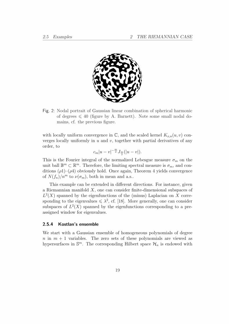
Fig. 2: Nodal portrait of Gaussian linear combination of spherical harmonicof degrees 6 40 (figure by A. Barnett). Note some small nodal do-mains, cf. the previous figure.

with locally uniform convergence in C, and the scaled kernel Kx,n(u, v) con-verges locally uniformly in u and v, together with partial derivatives of anyorder, to

cm|u− v|−m2 Jm

2(|u− v|).

This is the Fourier integral of the normalized Lebesgue measure σm on theunit ball Bm ⊂ Rm. Therefore, the limiting spectral measure is σm, and con-ditions (ρ1)–(ρ4) obviously hold. Once again, Theorem 4 yields convergenceof N(fn)/nm to ν(σm), both in mean and a.s..

This example can be extended in different directions. For instance, givena Riemannian manifold X, one can consider finite-dimensional subspaces ofL2(X) spanned by the eigenfunctions of the (minus) Laplacian on X corre-sponding to the eigenvalues 6 λ2, cf. [18]. More generally, one can considersubspaces of L2(X) spanned by the eigenfunctions corresponding to a pre-assigned window for eigenvalues.

2.5.4 Kostlan’s ensemble

We start with a Gaussian ensemble of homogeneous polynomials of degreen in m + 1 variables. The zero sets of these polynomials are viewed ashypersurfaces in Sm. The corresponding Hilbert space Hn is endowed with

19


the scalar product

〈f, g〉 =∑

|J |=n

(n

J

)−1

fJgJ , (8)

where

f(X) =∑

|J |=n

fJXJ , g(X) =∑

|J |=n

gJXJ , XJ = xj00 xj1

1 xj22 ... xjm

m ,

and

J = (j0, j1, j2, ... , jm), |J | = j0+j1+j2+ ... +jm,

(n

J

)=

n!

j0!j1!j2! ... jm!.

The form of the scalar product (8) comes from the complexification: afterthe continuation of the homogeneous polynomials f and g to Cm+1, up toa factor depending on n and m, it coincides with the scalar product in theFock-Bargmann space,

〈f, g〉 = cn,m

∫

Cm+1

f(Z)g(Z)e−|Z|2

d vol(Z) .

It is known that the complexified Kostlan ensemble is the only unitarilyinvariant Gaussian ensemble of homogeneous polynomials. On the otherhand, there are many other orthogonally invariant Gaussian ensembles, allof them having been classified by Kostlan [11].

The normalized covariance kernel of Kostlan’s ensemble equals(

X · Y|X| |Y |

)n

= (x · y)n = cosn Θ(x, y) .

This is a Hermitian positive definite kernel on Sm, and it is not difficult tocheck that it is the reproducing kernel in the Hilbert space

Hn =f : f(X) = |X|−nf(X), f ∈ Hn

with the scalar product borrowed from Hn.For Kostlan’s ensemble, the choice of the scaling parameter is different

from the one used in the previous examples: it is the square root of thedegree, not the degree itself. We put

Kx,n(u, v) = K(Φx(n

−1/2u), Φx(n−1/2v)

)= cosn Θ

(Φx(n

−1/2u), Φx(n−1/2v)

).

20

3 PROOFS

Noting that Θ(Φx(n

−1/2u), Φx(n−1/2v)

)is close to n−1/2|u−v| as n →∞, we

find that the scaled kernel converges to the kernel e−12|u−v|2 locally uniformly,

together with partial derivatives of any order. Thus, the limiting spectralmeasure is the Gaussian measure γm on Rm with the density exp

[−12|λ|2],

and Theorem 4 yields convergence of n−m2 N(fn) to ν(γm) both in mean and

a.s..An interesting feature of Kostlan’s ensemble is the very rapid off-diagonal

decay of its covariance.

3 The Riemannian case: the proofs

First, we explain the main steps in the proof of the local theorem, and thenturn to the proof of Theorem 4, which is based on the local version.


We fix the point x ∈ X, and denote by Fx the corresponding limiting Gaus-sian function. We also fix the following parameters:

• an arbitrarily small parameter δ, which will control the probabilities of theevents we discard;

• R > 1, which will be sent to infinity only at the very last step of the proof;

• a sufficiently big M , which controls the C2-norms: E‖fx,L‖C2(B(2R)) 6 Mand E‖Fx‖C2(B(2R)) 6M .

3.1.1 Coupling

The Gaussian functions fx,L and Fx are defined on different probabilityspaces, and we only know that their covariances are close. First of all, weneed to couple them, i.e., to find Gaussian functions fx,L and Fx defined onthe same probability space, equidistributed with fx,L and Fx correspondingly,and with high probability close to each other in C1(B(2R)). The C1-errorof coupling is controlled by a small parameter β(δ, R), whose value will befixed later.

Lemma 4. Given α > 0, there exist Gaussian functions fx,L and Fx definedon the same probability space and equidistributed with fx,L and Fx, such that,for L > L0(α, δ,R),

E‖fx,L − Fx‖C1(B(2R)) < α .

21

3.1 Proof of Theorem 5 3 PROOFS

Sketch of the proof of Lemma 4: We fix a finite η-net in B(2R) with suffi-ciently small η. First, using a simple finite-dimensional linear algebra argu-ment, we couple the restrictions of fx,L and Fx to this net and get the func-

tions fx,L and Fx, which are close to each other on the net. Then, using onceagain a simple linear algebra argument, but this time an infinite-dimensionalone, we extend the coupled random functions from the net to the whole ballB(2R). At last, using a priori estimates of the C2-norm of these functionsand the classical Hadamard-Landau inequality, we conclude that they closeto each other in C1(B(2R)). 2

Given β > 0, we introduce the event

Ω1 = ‖fx,L − Fx‖C1(B(2R)) > β .

Applying Lemma 4, we assume that the scaling parameter L is so big thatP(Ω1) < δ. Then we consider the events

Ω2 =‖fx,L‖C2(B(2R)) > δ−1M

, Ω3 =

‖Fx‖C2(B(2R)) > δ−1M

.

Each of them has probability at most δ. Discarding these events, we assumethat

‖fx,L‖C2(B(2R)) < δ−1M , ‖Fx‖C2(B(2R)) < δ−1M .

3.1.2 Stability

Discarding the events Ω1, Ω2, and Ω3, we get smooth functions fx,L and Fx

defined on the same probability space that are C1-close to each other. Wewish to conclude that the numbers of connected components of their zero setsare also close. Generally speaking, a C1-perturbation of a smooth functioncan drastically change the topology of its zero set. The good news is thatthis does not happen if the function and its gradient are not simultaneouslysmall. We call such functions stable. The next step is to show that, withhigh probability, the functions fx,L and Fx are stable.

Consider the event

Ω4 =

minu∈B(2R)

max |fx,L(u)|, |∇fx,L(u)| 6 2β

.

Lemma 5. Given δ > 0 and R > 0, there exist β = β(δ, R, M) and L0 =L0(δ, R), such that P(

Ω4

)< δ provided that L > L0.

22


Note that discarding the event Ω4 we also have

minB(2R)

max|Fx|, |∇Fx| > β .

The proof of Lemma 5 is based on the following simple and useful observation:

• if a C1-Gaussian function g has a constant variance, then the randomvariables g(u) and ∇g(u) are independent at each point u.

Sketch of the proof of Lemma 5: We choose a finite η-net yj in B(2R)with sufficiently small η = η(δ, R). Suppose that, for some y ∈ B(2R), both|fx,L(y)| and |∇fx,L(y)| are less or equal than 2β. Then, for some point yi ofthe net,

|fx,L(yi)| . β + δ−1Mη2 , |∇fx,L(yi)| . β + δ−1Mη .

Using the aforementioned independence (and non-degeneracy of the distri-bution of the Gaussian vector ∇fx,L), we estimate the probability that bothevents occur simultaneously, and take the union bound over the net. 2

3.1.3 Stable components of the zero set

Discarding events Ωi, 1 6 i 6 4, we have, for sufficiently large L,

‖fx,L − Fx‖C1(B(2R)) < β ,

while

minB(2R)

max|fx,L|, |∇fx,L| > β , minB(2R)

max|Fx|, |∇Fx| > β .

We claim that this yields

N(R− 1; Fx) 6 N(R, fx,L) 6 N(R + 1; Fx) . (9)

Combined with Theorem 1, this yields Theorem 5.

To prove (9), we will use a lemma from multivariable calculus. Denoteby V+t an open t-neighbourhood of the set V ⊂ Rm.

Lemma 6. Fix positive α and β. Let f be a C1-smooth function on anopen ball B ⊂ Rm such that at every point u ∈ B, either |f(u)| > α, or|∇f(u)| > β. Then each component γ of the zero set Z(f) with dist(γ, ∂B) >

23


α/β is contained in an open “annulus” Aγ ⊂ γ+α/β bounded by two smoothconnected hypersufaces such that f = +α on one boundary component ofAγ, and f = −α on the other. Furthermore, “the annuli” Aγ are pairwisedisjoint.

Proof of Lemma 6: With no loss of generality, we assume that α = β = 1(otherwise, we replace the function f by λ1f(λ2u) with appropriate λ1 andλ2). We fix the component γ, as in the assumptions. Given t ∈ (0, 1],we denote by γt a connected component of the sublevel set |f | < t thatcontains γ, and look at the evolution of γt as t grows from 0 to 1. During thisevolution |∇f | > 1, therefore, the component γt neither merges with othercomponents of the set |f | < t, nor shrinks.

Using once again that |∇f | > 1 everywhere on the component γt, wesee that γt ⊂ γ+1, and therefore, during the evolution γt cannot reach theboundary ∂B. 2

As an immediate corollary, we get the needed stability of components ofthe zero set:

Lemma 7. Let the function f meet assumptions of Lemma 6 and let g beany C(B)-function with sup |g| < α. Then each component γ of Z(f) withdist(γ, ∂B) > α/β generates a component γ of the zero set Z(f +g) such thatγ ⊂ γ+α/β. Different components γ1 6= γ2 of f generate different componentsγ1 6= γ2 of Z(f + g).

Now, applying Lemma 7 to the functions f = fx,L and g = Fx−fx,L withα = β, and then, once again, to the functions f = Fx and g = fx,L − Fx, weget (9). This completes the proof of Theorem 5. 2


For a.e. x ∈ X, denote by Fx the corresponding local limiting function. Then

ν(x) = limR→∞

EN(R; Fx)

vol B(R).

Since N(R; Fx) does not exceed the number of critical points of Fx in the ballB(R), by the Kac-Rice upper bound (Lemma 2), ν is a bounded function onX.

24


We need to show that

limL→∞

E∣∣∣L−mN(fL)−

∫

X

ν d volX

∣∣∣ = 0 .

Below, we will explain how we prove the upper bound

limL→∞

E[L−mN(fL)−

∫

X

ν d volX

]+

= 0 .

The proof of the lower bound is similar, but simpler, since it does not requirea separation of small and long components, which we will describe below.

3.2.1 Discarding long components

Long components are the ones whose diameter is much bigger than 1/L.They cannot be captured by our local approximation of the zero set Z(fL)by Z(Fx), so we need to discard them.

Definition 4. We call a connected component of the zero set Z(fL) D-longif diam(γ) > D/L, and denote by ND−long(fL) the number of D-long compo-nents of the zero set Z(fL).

Lemma 8. For D > 1, we have

limL→∞

L−m END−long(fL) . 1/D .

Sketch of the proof: We fix a D/(4L)-net on X of cardinality ' (L/D)m,cover X by balls Bj of radius D/(2L) centered at the points of this net,and bound the number of D-long components by the total number of criticalpoints of the restrictions fL

∣∣∂Bj

. To estimate the mean number of critical

points of these restrictions, we apply the Kac-Rice upper bound. 2

3.2.2 Discarding small components

Small components are boundary components of nodal domains6 of fL whosevolume is much smaller than L−m. Ignoring small components, we will beable to control the number of components by the volume of the set they arecontained in.

6 Nodal domains of fL are connected components of the set fL 6= 0.

25


Definition 5. We call a nodal domain G of the function fL δ-small ifvolX(G) < δL−m. We call a connected component γ of the zero set Z(fL)δ-small if it is a boundary component of a δ-small nodal domain. We denoteby Nδ−small(fL) the number of δ-small components of Z(fL).

Lemma 9. There exists a constant c > 0 such that

limL→∞

L−m ENδ−small(fL) . δc .

To prove this lemma, we use a chain of four lemmas on (non-random)smooth functions. The starting point is Morrey’s version of Poincare’s in-equality [6, Section 4.5.3]:

Lemma 10. Suppose H is a smooth function in the unit ball B ⊂ Rm. Then,for q > m,

supB|H −H(0)| 6 C(m, q)‖DH‖Lq(B).

As a corollary, we get

Lemma 11. Let B ⊂ X be a ball centered at c of a sufficiently small radius.Suppose that f ∈ C2(B), Df(c) = 0, and f vanishes somewhere on theboundary ∂B. Then, for q > m,

‖Df‖C(B) .(volX(B)

) 1m− 1

q ‖D2f‖Lq(B)

and‖f‖C(B) .

(volX(B)

) 2m− 1

q ‖D2f‖Lq(B) .

Next, it is convenient to introduce the notation

I(B) =

∫

B

|D2f |q d volX .

The previous lemma yields the following one:

Lemma 12. Under the assumptions of the last lemma, we have

I(B)−s .(volX(B)

)t∫

B

|f |−(1−ε)|Df |−(m−ε) d volX ,

where ε > 0 is so small and q > m is so large that the parameters

s =m + 1− 2ε

q, t = (1− ε)

( 2

m− 1

q

)+ (m− ε)

( 1

m− 1

q

)− 1

are positive.

26


For a smooth function f on X, we denote by N = Nf (δ) the numberof nodal domains of f of volume less than δ. Note that if f has N nodaldomains of volume less than δ, then we can find N disjoint balls Bj so that

• the gradient of f vanishes at the center of each ball Bj;

• the function f vanishes somewhere on the boundary of each ball Bj;

• the volume of each ball Bj is less than δ.

Then Lemma 12 allows us to estimate from above the number of these balls:

Lemma 13. Given a positive integer m, there exist parameters q > m, ε > 0,c > 0, s > 0, such that, for any f ∈ C2(X),

Nf (δ) . δc(∫

X

|D2f |q d volX

) ss+1

(∫

X

|f |−(1−ε)|Df |−(m−ε) d volX

) 1s+1

.

We apply this estimate to the random function fL with δL−m instead of δ.Taking the expectation, applying Holder’s inequality, and using the smooth-ness and non-degeneracy of the ensemble (fL), as well as the independenceof fL(x) and DfL(x), we get Lemma 9.

3.2.3 Integral-geometric estimate for normal components

We fix a small parameter δ and a large parameter D.

Definition 6. We call the connected component γ of Z(fL) normal if it isneither δ-small, nor D-long. We denote by Nnorm(fL) the number of normalcomponents of the zero set of fL.

Keeping in mind Lemma 8 and Lemma 9, it suffices to show that

limL→∞

E[L−mNnorm(fL)−

∫

X

ν dvolX

]+

= 0 .

We start with a Riemannian version of the integral-geometric estimate 1.3.1.Denote by Nnorm(x, r; fL) the number of normal components of the zero setZ(fL) contained in the geodesic ball B(x; r) and by N∗

norm(x, r; fL) the numberof normal components of the zero set Z(fL) that intersect the geodesic ballB(x; r).

27


Lemma 14. Given ε > 0, there exists δ > 0 such that, for every r < δ,

(1− ε)

∫

X

Nnorm(x, r; fL)

vol B(R)d volX(x) 6 Nnorm(fL)

6 (1 + ε)

∫

X

N∗norm(x, r; fL)

vol B(R)d volX(x) . (10)

Here vol B(r) is the Euclidean volume of the m-dimensional ball of radius r.The proof of this lemma is very close to that of Lemma 1 and we skip it.

Since the diameters of normal components do not exceed D/L, we have

N∗norm(x, r; fL) 6 Nnorm(x, r + L−1D; fL) .

Next, we fix a sufficiently big R, put D =√

R, and use the right half ofestimate (10) with r = R/L, where L is big enough. We get

Nnorm(fL)

Lm6 (1 + 2ε)

∫

X

Nnorm(x, (R + D)/L; fL)

vol B(R + D)d volX(x) .

Using the left half of estimate (10), we see that the integral

∫

X


vol B(R + D)d volX(x)

is majorized by the total number of critical points of the function fL. In turn,by the smoothness assumption and the Kac-Rice estimate, the expectationof the latter number is . Lm volX(X). Therefore,

E[L−mNnorm(fL)−

∫

X

ν d volX

]+

6∫

Ω

∫

X

[Nnorm(x, (R + D)/L; fL)

vol B(R + D)− ν(x)

]+

d volX(x) dP(ω) + O(ε) .

Thus, it remains to estimate the double integral on the RHS.

3.2.4 Completing the proof of Theorem 4

To simplify notation, we assume that volX(X) = 1. Put

Ωx,R,L(ε) =∣∣∣N(x,R/L; fL)

vol B(R)− ν(x)

∣∣∣ > ε

.

28

4 MONOCHROMATIC WAVES

By Theorem 5, for a.e. x ∈ X,

limR→∞

limL→∞

PΩx,R+D,L(ε)

= 0 .

Applying Egorov’s theorem to this double limit, we see that, given η > 0,there exists a set Xη ⊂ X with vol(Xη) > 1− η, such that the convergence isuniform on Xη, that is,

limR→∞

limL→∞

supx∈Xη

PΩx,R,L(ε)

= 0 .

Since we have discarded δ-small components (and since D =√

R),

Nnorm(x, (R + D)/L; fL) . δ−1 vol B(R + D) .

Therefore, uniformly in ω ∈ Ω,∫

X\Xη


vol B(R + D)d volX(x) . ηδ−1 ,

and uniformly in x ∈ X,∫

Ωx,R+D,L(ε)


vol B(R + D)dP(ω) . δ−1P

Ωx,R+D,L(ε).

The remaining integral is small by the very definition of the set Ωx,R+D,L(ε):∫

Ω\Ωx,R+D,L(ε)

∫

Xη

[Nnorm(x, (R + D)/L; fL)

vol B(R + D)− ν(x)

]+

d volX(x) dP(ω) 6 ε .

It remains to let L →∞, R →∞, η → 0, δ → 0, and then ε → 0. 2

4 Random monochromatic waves

In this lecture, we will discuss the nodal portraits of two-dimensional randomfunctions f satisfying the Helmholtz equation ∆f + κ2f = 0. We considertwo instances closely related to each other:

• The random ensemble of two-dimensional spherical harmonics, which wehave already discussed in 2.5.2.

• The Gaussian Helmholtz waves. These are translation-invariant Gaussianfunctions on R2 whose spectral measure is the Lebesgue measure on the unitcircle S1.

Recall that the Gaussian Helmholtz wave is the limiting function for theensemble of two-dimensional spherical harmonics.

29

4.1 Bond percolation model 4 MONOCHROMATIC WAVES

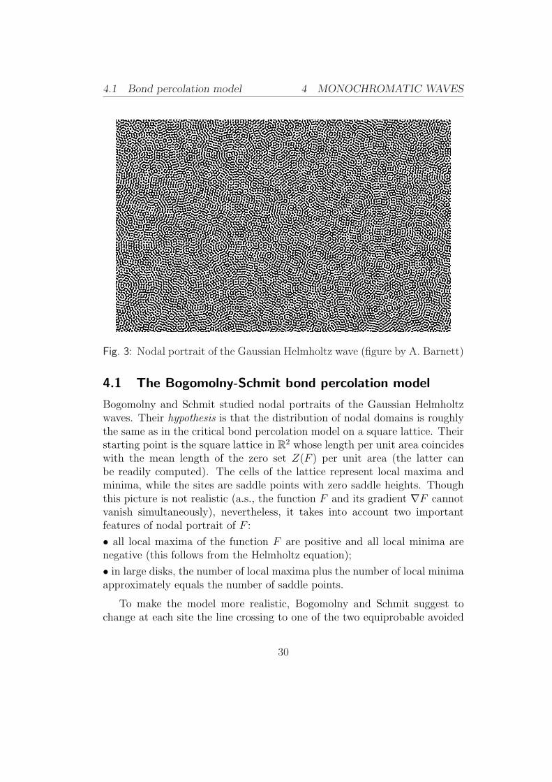
Fig. 3: Nodal portrait of the Gaussian Helmholtz wave (figure by A. Barnett)

4.1 The Bogomolny-Schmit bond percolation model

Bogomolny and Schmit studied nodal portraits of the Gaussian Helmholtzwaves. Their hypothesis is that the distribution of nodal domains is roughlythe same as in the critical bond percolation model on a square lattice. Theirstarting point is the square lattice in R2 whose length per unit area coincideswith the mean length of the zero set Z(F ) per unit area (the latter canbe readily computed). The cells of the lattice represent local maxima andminima, while the sites are saddle points with zero saddle heights. Thoughthis picture is not realistic (a.s., the function F and its gradient ∇F cannotvanish simultaneously), nevertheless, it takes into account two importantfeatures of nodal portrait of F :

• all local maxima of the function F are positive and all local minima arenegative (this follows from the Helmholtz equation);

• in large disks, the number of local maxima plus the number of local minimaapproximately equals the number of saddle points.

To make the model more realistic, Bogomolny and Schmit suggest tochange at each site the line crossing to one of the two equiprobable avoided

30

4.1 Bond percolation model 4 MONOCHROMATIC WAVES

+

−

−

+ −

+−

− +

−+

+

Fig. 4: Avoided nodal crossings in the Bogomolny-Schmit model

crossings, as shown in Fig 4.1. At different sites, the changes are independent.Then Bogomolny and Schmit introduce two dual square lattices: the

‘blue’ one, with vertices at the cells of the grid where the function is positive,and the ‘red’ one, with vertices at the cells of the grid where the function isnegative. Each realization of the random choice of avoided crossings gener-ates two graphs, the blue one, whose vertices are the blue lattice points andthe red one, whose vertices are the red lattice points. Two vertices are con-nected by an edge if the corresponding cells of the grid belong to the samenodal domain of the random function. Each of these graphs uniquely de-

Fig. 5: Bond percolation on the ‘blue’ lattice

termines the topology of the whole nodal portrait (so it suffices to consideronly one of them), and each of them represents the critical bond percola-tion on the corresponding square lattice. Then using some heuristics comingfrom statistical mechanics, Bogomolny and Schmit computed the limits ofthe mean 7,

limR→∞

EN(R; F )

R2=

3√

3− 5

π≈ 0.0624 .

7 as we have already mentioned, Konrad’s thesis [10] puts some doubt about this exactvalue

31

4.2 Exponential concentration 4 MONOCHROMATIC WAVES

They also argued that the growth of the variance of N(R; F ) is proportionalto R2 and that fluctuations of the random variable N(R; F ) are asymptoti-cally Gaussian when R →∞. They concluded their work with a remarkableprediction of the power distribution law for the areas of nodal domains, basedon percolation theory.

The major problem with this model is that it completely ignores correla-tions between values of the function F , which decay only as the distance tothe power −1

2. The ‘minor’ problem is that there is still no rigorous mathe-

matical treatment of the critical bond percolation on the square lattice.

Question 4. Reveal “a hidden universality law” that provides a rigorousfoundation for the Bogomolnny-Schmit work.

It seems that, at present, we are very far from understanding this universality.We do not have answers to the following, much more basic questions:

Question 5. Show that with probability one the zero set Z(F ) has no infinitecomponent.

Question 6. Show that for each ε > 0, the probability that the setx : F (x) >

ε, |x| < R

has a component of diameter bigger than εR tends to zero asR →∞.

In one aspect, we went beyond the Bogomolny-Schmit predictions. Namely,for random Gaussian monochromatic waves, we can rigorously prove the ex-ponential concentration of the number of connected components around itsmean value. Contrary to the Bogomolny-Schmit model, this result is not par-ticularly two-dimensional. To simplify the exposition, we restrict ourselvesto the ensemble of two-dimensional spherical harmonics.

4.2 Exponential concentration

Here, Hn is the 2n + 1-dimensional subspace of L2(S2) consisting of thereal-valued spherical harmonics of degree n on S2. This is the space of eigen-functions of the Laplace-Beltrami operator on S2 with the n-th eigenvalueλn = n(n + 1). An alternative definition says that the elements of this spaceare restrictions of harmonic homogeneous polynomials in R3 to the sphereS2. By (fn) we denote the ensemble of random Gaussian spherical harmonicsof degree n built on the space Hn. Recall that the limiting spectral mea-sure for this ensemble is the Lebesgue measure ω on the unit circumference

32


S1 ⊂ R2 and that the limiting translation-invariant function is the GaussianHelmholtz wave. According to Theorem 4, N(fn)/n2 converges to a positiveconstant ν(ω) both in mean and a.s., and according to the Bogomolny-Schmitprediction, ν(ω) = (3

√3− 5)/π.

Theorem 6. For every ε > 0, there exist positive constants c(ε) and C(ε)such that

P∣∣∣N(fn)

n2− ν(ω)

∣∣∣> ε

6 C(ε)e−c(ε)n .

The exponential concentration in Theorem 6 can be viewed as anothermanifestation of Levy’s concentration of measure principle. It is particu-larly interesting, since the covariance of the ensemble of Gaussian sphericalharmonics has a very slow off-diagonal decay.

The proof of Theorem 6 is based on the Gaussian isoperimetric inequality,which was independently found by Sudakov and Tsirelson [20] and Borell [4].

4.2.1 Gaussian isoperimetry

Put d = 2n + 1. It is convenient to view the Hilbert space Hn as a d-dimensional Euclidean space equipped with a standard Gaussian measure γd

with E|x|2 = 1. As above, by V+% we denote an open %-neighbourhood of theset V ⊂ Rd.

Theorem 7 (Borell, Sudakov-Tsirelson). Suppose V ⊂ Rd is a Borel setand Π ⊂ Rd is an affine half-space such that γd(V ) = γd(Π). Then, for every% > 0, γd(V+%) > γd(Π+%).

A simple computation shows that if γd(Π+%) is not too close to 1, thenγd(Π) must be exponentially small in d, like exp[−c%2d]. Returning to thespace Hn of spherical harmonics, we get

Corollary 1 (Levy’s concentration of Gaussian measure onHn). Let V ⊂ Hn

be any Borel set of spherical harmonics. Suppose that the set V+% satisfiesP(V+%) 6 3

4. Then P(V ) 6 2e−c%2n.

To use the concentration of measure principle, we need to show that thenumber N(f) doesn’t change too much under small perturbation of f in theL2(S2)-norm. Certainly, it is not true for all f ∈ Hn, but we show that the“unstable” spherical harmonics f ∈ Hn for which small perturbations canlead to a drastic decrease in the number of components of the zero set areexponentially rare.

33


4.2.2 Uniform lower semicontinuity of N(f)/n2 outside a smallexceptional set

Here is a fundamental lemma. It gives a quantitative version of estimates wewere using in the course of the proof of Theorem 5.

Lemma 15 (Uniform lower semi-continuity of N(fn)/n2). For every ε > 0,there exist % > 0 and an exceptional set E ⊂ Hn of probability P(E) 6C(ε)e−c(ε)n, such that for all f ∈ Hn \ E and for all g ∈ Hn satisfying‖g‖ 6 %, we have

N(f + g) > N(f)− εn2.

A seeming asymmetry in this statement appears since we perturb non-exceptional spherical harmonics by arbitrary ones with small norm.

Theorem 6 readily follows from this lemma combined with the previousresults. Indeed, denote by mn the median of the random variable N(f)/n2.By Theorem 4, we have mn → ν(ω) as n →∞. Therefore, it suffices to showthat

P∣∣∣N(f)

n2−mn

∣∣∣ > ε

< C(ε)e−c(ε)n2

.

First, we consider the set V =f ∈ Hn : N(f) > (mn + ε)n2

. Then for

f ∈ (V \ E)+% we have N(f) > mnn2, and therefore P(

(V \ E)+%

)6 1

2.

Hence, by the concentration of Gaussian measure, P(V \ E) 6 2e−c%2n, andfinally

P(V ) 6 P(V \ E) + P(E) 6 2e−c%2n + C(ε)e−c(ε)n 6 C(ε)e−c(ε)n .

Now, let us look at the set V =f ∈ Hn : N(f) < (mn− ε)n2

. For this set,

V+% ⊂f ∈ Hn : N(f) < mnn

2 ∪ E, so that

P(V+%) 6 1

2+ C(ε)e−c(ε)n <

3

4

for large n, and it follows that P(V ) 6 2e−c%2n. This proves Theorem 6modulo Lemma 15. 2

The proof of Lemma 15 goes in two steps. First, we single out the ex-ceptional set E of unstable spherical harmonics and estimate its measure.Then we show that the number of connected components of non-exceptionalspherical harmonics is stable under small perturbations.

34


4.2.3 Several facts about spherical harmonics

We start with a few standard facts about spherical harmonics of degree n,which will be used in the proof of Lemma 15. These facts can be derivedeither from the fact that they are eigenfunctions of the Laplacian on thesphere corresponding to the eigenvalue n(n + 1), or from the fact that theyare traces of homogeneous harmonic polynomials in R3 of degree n on theunit sphere. Everywhere below we assume that n > 1.

Lemma 16 (Mean-value property). For any f ∈ Hn and any point x ∈ S2,we have

|f(x)|2 . n2

∫

D(x,1/n)

f 2 .

Here D(x, 1/n) is a spherical disc of radius 1/n centered at x.

Lemma 17 (Length estimate). For any f ∈ Hn that is not identically 0, thetotal length of Z(f) does not exceed Cn.

The next lemma follows from the classical Faber-Krahn inequality:

Lemma 18 (Area estimate). For any connected component G of S2 \Z(f),we have Area(G) & n−2.

Actually, it is not difficult to show that every nodal domain of f contains adisc of radius c/n.

4.2.4 Spherical harmonics with many unstable disks

Here, we use an idea similar to the one used in the proof of Theorems 5and 4: the nodal portrait of a spherical harmonic is unstable under smallperturbations only if in many different places on the sphere S2 the functionf and its gradient ∇f are simultaneously small.

We fix small positive parameters α and δ and a large positive parameterR; all of them will be some powers of ε. Then we cover the sphere S2 by' R−2n2 disks Dj of radius R/n in such a way that the concentric disks 4Dj

with 4 times larger radius cover the sphere with a bounded multiplicity. Wedenote by D the collection of the discs Dj.

Definition 7 (unstable disks). We call the disk Dj stable, if for each x ∈ 3Dj

either |f(x)| > α, or |∇f(x)| > αn. Otherwise, the disk Dj is unstable.

35


Definition 8 (exceptional spherical harmonics). We call the spherical har-monic f ∈ Hn exceptional, if the number of unstable disks is at least δn2,and denote by E the set of all exceptional spherical harmonics of degree n.

Lemma 19. Given δ > 0, there exist positive small α0(δ) and c(δ), and apositive large C(δ) such that

P(E) 6 C(δ)e−c(δ)n

provided that α 6 α0(δ).

We skip the proof of this lemma (it is given in Section 4.2 of [16]), butnote that, curiously enough, it uses once again the concentration of measureprinciple.

4.2.5 Proof of the uniform lower semicontinuity

Fix a “stable” spherical harmonic f ∈ Hn \E. We need to show that at mostεn2 components of the zero set Z(f) can disappear after perturbation of f byanother spherical harmonic g ∈ Hn with sufficiently small L2-norm ‖g‖ < %.First, in several steps, we identify possibly ‘unstable’ connected componentsof the zero set Z(f) that can disappear after perturbation, show that theirnumber is small compared to n2, and discard them. Then Lemma 7 willyield that all other connected components of Z(f) do not disappear after theperturbation.

• First, we discard the nodal components γ whose diameter is bigger thanR/n. By the length estimate in Lemma 17, their number is . R−1n2, whichis small compared to n2.

With each remaining component γ of the nodal set Z(f) we associate adisk Dj from the collection D such that Dj ∩ γ 6= ∅. Then γ ⊂ 2Dj. Bythe area estimate in Lemma 18, the number of components γ intersecting Dj

(and, thereby, contained in 2Dj) is bounded.

• Second, we discard the components γ with unstable disks Dj. Since f is notexceptional, and since, by the area estimate, each disk Dj cannot intersecttoo many components contained in 2Dj, the number of such components isalso small compared to n2.

• At last, we discard the components γ such that

max3Dj

|g| > α .

36

4.3 More questions 4 MONOCHROMATIC WAVES

To estimate the number N of such disks, we denote by D∗j ⊂ 4Dj the disk of

radius 1/n centered at the point yj where |g| attains its maximum in 3Dj.By Lemma 16, ∫

D∗j

|g|2 & n−2|g(yj)| = α2n−2 ,

whence%2 > ‖g‖L2(S2) & Nα2n−2 ,

that is, N . %2α−2n2. As above, using Lemma 18 and juxtaposing theareas, we conclude that the number of components γ affected by this is. R2N . R2%2α−2n2, which is much less than εn2, provided that %2 is muchless than εα2R−2.

In the three steps above, we have discarded at most εn2 connected com-ponents of Z(f). Let γ be one of the remaining components. By our con-struction, there is a disc Dj so that

• γ ⊂ 2Dj;

• max(|f |, n−1|∇f |) > α everywhere in 3Dj;

• |g| < α everywhere in 3Dj.

Then, by Lemma 7, the component γ survives when we perturb the functionf by g. This completes the proof of Lemma 15. 2

4.3 More questions

Question 7. Is it possible to extend the exponential concentration result torandom functions that do not solve the Helmholtz equation?

This question is open even in the one-dimensional case, that is, for zerocrossings of sufficiently smooth Gaussian stationary processes on R1, cf.Tsirelson’s lecture notes [22]. The principal obstacle are small nodal do-mains.

Nothing is known about the number of connected components of thezero set for a ‘randomly chosen’ high-energy Laplace eigenfunction fλ onan arbitrary compact surface X without boundary endowed with a smoothRiemannian metric g. It is tempting to expect that Theorem 6 models what ishappening when X is the two-dimensional sphere S2 endowed with a genericRiemannian metric g that is sufficiently close (with several derivatives) to theconstant one. However, the following more naıve question is widely open:

37

References References

Question 8. Suppose X is the two-dimensional sphere S2 endowed with ageneric Riemannian metric g that is sufficiently close (with several deriva-tives) to the constant one. Denote by N(fλ) the number of connected com-ponents of the zero set of the Laplace eigenfunction fλ on X. Is it true thatlim sup

λ→∞N(fλ) = +∞?

Instead of perturbing the “round metric” on the sphere S2, one can adda small potential V to the Laplacian on the “ round sphere”. The questionremains just as hard.

References

[1] R. Adler, J. Taylor, Random fields and geometry. Springer Verlag, NewYork, 2007.

[2] J.-M. Azaıs, M. Wschebor, Level sets and extrema of random processesand fields. John Wiley & Sons Inc., Hoboken, NJ, 2009.

[3] E. Bogomolny, C. Schmit, Percolation model for nodal domainsof chaotic wave functions. Phys. Rev. Letters, 88 (2002), 114102.arXiv:nlin/0110019v1; Random wavefunctions and percolation, J.Phys. A 40 (2007), 14033–14043. arXiv:0708.4335v1

[4] C. Borell, The Brunn-Minkowski inequality in Gauss space. Invent. Math.30 (1975), 207–216.

[5] J. Bourgain, Z. Rudnick, Restriction of toral eigenfunctions to hy-persurfaces and nodal sets. Geom. Funct. Anal. 22 (2012), 878–937.arXiv:1105.0018

[6] L. Evans, R. Gariepy, Measure theory and fine properties of functions.Studies in Advanced Mathematics. CRC Press, Boca Raton, FL, 1992.

[7] D. Gayet and J.-Y. Welschinger, Exponential rarefaction of real curveswith many components. Inst. Hautes Etudes Sci. Publ. Math. 113 (2011),69–96. arXiv:1005.3228v1; What is the total Betti number of a ran-dom real hypersurface? arXiv:1107.2288v1; Betti numbers of ran-dom real hypersurfaces and determinants of random symmetric matrices,arXiv:1207.1579v1

38


[8] U. Grenander, Stochastic processes and statistical inference, Ark. Mat. 1(1950), 195–277.

[9] M. Hairer, An Introduction to Stochastic PDEs.http://www.hairer.org/notes/SPDEs.pdf

[10] K. Konrad, Asymptotic Statistics of Nodal Domains of Quantum ChaoticBilliards in the Semiclassical Limit, Dartmouth College, 2012.

[11] E. Kostlan, On the expected number of real roots of a system of randompolynomial equations, Foundations of computational mathematics (HongKong, 2000), 149-188, World Sci. Publ., River Edge, NJ, 2002.

[12] A. Lerario, E. Lundberg, Statistics on Hilbert’s Sixteenth Problem.arXiv:1212.3823.

[13] T. L. Malevich, Contours that arise when the zero level is crossed byGaussian fields. Izv. Akad. Nauk UzSSR Ser. Fiz.-Mat. Nauk 16 (1972),20–23.

[14] J. Marzo, Marcinkiewicz-Zygmund inequalities and interpolationby spherical harmonics. J. Funct. Anal. 250 (2007), 559–587.arXiv:math/0611503

[15] M. Nastasescu, The number of ovals of a real plane curve. Senior Thesis,Princeton University, 2011.

[16] F. Nazarov, M. Sodin, On the number of nodal domains of ran-dom spherical harmonics. Amer. J. Math. 131 (2009), 1337–1357.arXiv:0706.2409v1

[17] F. Nazarov, M. Sodin, On the number of connected components of thezero sets of smooth random functions, in preparation.

[18] L. Nicolaescu, The blowup along the diagonal of the spectral function ofthe Laplacian. arXiv:1103.1276

[19] P. Sarnak, Letter to B. Gross and J. Harris on ovals of random planecurves, May 2011. http://publications.ias.edu/sarnak/paper/510

39


[20] V. N. Sudakov and B. Tsirel’son, Extremal properties of half-spaces forspherically invariant measures. Problems in the theory of probability dis-tributions, II. Zap. Naucn. Sem. Leningrad. Otdel. Mat. Inst. Steklov.(LOMI) 41 (1974), 14–24. (Russian)

[21] G. Szego, Orthogonal polynomials. Fourth edition. American Mathemat-ical Society, Colloquium Publications, Vol. XXIII. American Mathemat-ical Society, Providence, R.I., 1975.

[22] B. Tsirelson, Gaussian measures. Lecture notes. Tel Aviv University,Fall 2010.http://www.tau.ac.il/~tsirel/Courses/Gauss3/main.html

[23] B. Tsirelson, Measurability and continuity. Lecture notes. Tel Aviv Uni-versity, Fall 2012.http://www.tau.ac.il/~tsirel/Courses/MeasCont/main.html

[24] N. Wiener, The ergodic theorem, Duke Math. J. 5 (1939), 1–18.

40

Documents

Lectures on random nodal portraits (Sodin) - TAUsodin/SPB-Lecture-Notes.pdf · Lectures on random nodal portraits Mikhail Sodin School of Mathematics Tel Aviv University Tel Aviv