ECE 645: Estimation Theory

Spring 2015

Instructor: Prof. Stanley H. Chan

Lecture Note 1: Bayesian Decision Theory

(LaTeX prepared by Stylianos Chatzidakis)March 31, 2015

This lecture note is based on ECE 645(Spring 2015) by Prof. Stanley H. Chan in the School ofElectrical and Computer Engineering at Purdue University.

1 Introduction

Classification appears in many disciplines for pattern recognition and detection methods. In thislecture we introduce the Bayesian decision theory, which is based on the existence of prior distri-butions of the parameters.

1.1 Bayesian Detection Framework

Before we discuss the details of the Bayesian detection, let us take a quick tour about the overallframework to detect (or classify) an object in practice. In the Bayesian setting, we model obser-vations as random samples drawn from some probability distributions. The classification processusually involves extracting features from the observations, and a decision rule that satisfies certainoptimality criterion. See Figure 1.

Measurement Feature Extraction Classifier Classification

Figure 1: Block diagram of a classifier

When the distributions of the random samples are not known (which is true in most real-worldapplications), we might need an estimation algorithm to first determine the parameters of thedistributions, e.g., mean and standard deviation. A decision rule can then designed based on theseestimated parameters. To verify the efficiency of the classifier, testing data are used to calculatethe error rate or false alarm rate. In most cases, a classifier with small false alarm rate is sought.This process is shown in Figure 2.

Measurement Feature Extraction Classifier Classification

Estimation Algorithm Training Data

Figure 2: classifier

In practice, of course, all the above building blocks have to be taken into account. However, tohelp us understand the important ideas of the detection theory, we will focus on the design of the

classifiers in this course. Interested readers can consult standard textbooks on pattern recognitionsfor detailed discussions on these practical issues.

1.2 Objectives and Organizations

We begin this lecture note with a brief review of probability. We assume that readers are familiarwith introductory probability theory (e.g., ECE 600). After reviewing probability theory, we willdiscuss the general Bayes’ decision rule. Then, we will discuss three special cases of the generalBayes’ decision rule: Maximum-a-posteriori (MAP) decision, Binary hypothesis testing, and M-aryhypothesis testing.

2 Review of Probability

2.1 Probability Space

Any random experiment can be defined using the probability space (S,F ,P) where S is the samplespace, F is the event space, and P is the probability mapping. The sample space S is a non-emptyset containing all outcomes of the experiments. The event space F is a collection of subsets of Sto which probabilities are assigned. The event space F must be a non-empty set that satisfies theproperties of a σ-field. The probability mapping is a set function that assigns a real number toevery set:

P : F → R (1)

and must satisfy the following three probability axioms:

Non-negativity: P(A) ≥ 0, for all A ∈ FNormalization: P(S) = 1Additivity: P(A ∪B) = P(A) + P(B) if A ∩B = ∅.

2.2 Conditional Probability

In many situations we would want to know the probability of an event A occurring given thatanother event B has occurred. In this case, the probability of an event A given that another eventB has occured is called conditional probability. The condition probability of A given B is definedas:

P(A|B) =P(A ∩B)

P(B)(2)

assuming P(B) > 0.

Example 1.

Consider rolling a die. The probability of event A = 6 is equal to 1/6. However, if someoneprovides additional information, let’s say that the event B =roll of a die was bigger than 4, thenthe probability of A given B is:

P(A|B) =P(A ∩B)

P(B)=

1/6

3/6= 1/3.

2

A simple calculation of conditional probability allows us to write:

P(A ∩B) = P(A|B)P(B) (3)

andP(B ∩A) = P(B|A)P(A) (4)

then equating the left and right hand sides we can derive the Bayes’ Theorem:

Theorem 1. Bayes’ Theorem

For any events A and B such that P(B) > 0,

P(A|B) =P(B|A)P (A)

P(B). (5)

The Bayes’ theorem can be generalized to yield the following result.

Theorem 2. Law of Total Probability

If A1, A2, . . . , An is a partition of the sample space and B is an event in the event space, then

P(B) =

n∑

i=1

P(B|Ai)P(Ai) (6)

The law of total probability suggests that for any event B, we can decompose B into a sum ofn disjoint subsets Ai. Moreover, applying the total probability law to Bayes theorem yields

P(A|B) =P(B|A)P (A)

∑ni=1 P(B|Ai)P(Ai)

(7)

for A,B ∈ F , P(A) > 0 and P(B) > 0.

2.3 Random Variables

A random variable is a real function from the sample space to the real numbers:

X : S → R (8)

A random variable can be discrete or continuous. For the discrete case, the probability massfunction is defined as

pX(x) = P(ω ∈ S : X(ω) = x) (9)

For the continuous case, the cumulative distribution function is defined as

FX(x) = P(ω ∈ S : X(ω) ≤ x) (10)

When the cumulative distribution function is differentiable, we can define the probability densityfunction as

fX(x) =d

dxFX(x). (11)

3

2.4 Expectations

The expectation of a random variable described by a probability mass function or a probabilitydensity function is

E[X] =

{

∑

xpX(x), if X is discrete,∫∞−∞ xfX(x)dx, if X is continuous.

(12)

The conditional expectation is

E[X|Y = y] =

∫ ∞

−∞xfX|Y (x|y)dx (13)

The variance is defined as:

Var[X] = E[(X − E[X])2] = E[X2]− E[X]2. (14)

A very useful result of the expectation is the total expectation formula, also known as theiterated expectation.

Theorem 3. Total Expectation

E[X] = EY [EX|Y [X|Y = y]] (15)

Proof.

E[X] =

∫ ∞

−∞xfX(x)dx =

∫ ∞

−∞x

∫ ∞

−∞fXY (x, y)dxdy

=

∫ ∞

−∞x

∫ ∞

−∞fX|Y (x|y)dydx

=

∫ ∞

−∞fY (y)

∫ ∞

−∞xfX|Y (x|y)dx

=

∫ ∞

−∞E[X|Y = y]fY (y)dy = EY [EX|Y [X|Y = y]].

✷

2.5 Gaussian Distribution

Finally we review the Gaussian distribution. A single variable Gaussian distribution is defined as

fX(x) =1√2πσ

e−1

2

(

x− µ

σ

)2

, (16)

where µ is the mean and σ2 is the variance. We write

X ∼ N (µ, σ2) (17)

to denote a random variable X drawn from a Gaussian distribution.

4

For multivariate Gaussian, the distribution is

fX(x) =1

(2π)d/2|Σ|1/2 exp

{

−1

2(x− µ)TΣ−1(x− µ)

}

, (18)

where X = [X1,X2, · · · ,Xd]T is a d-dimensional vector, µ = [µ1, µ2, · · · , µd]

T is the mean vector,and

Σ = E[(X − µ)(X − µ)T ] =

Var(X1) · · · Cov(X1,Xd)...

. . ....

Cov(X1,Xd) · · · Var(Xd)

(19)

is the covariance matrix.If Cov(Xi,Xj) = 0 then Xi and Xj are said to be uncorrelated. If Cov(Xi,Xj) > 0 then

Xi and Xj are said to be positively correlated. However, it should be clarified that uncorrelateddoes not imply independent, because Cov(X,Y ) = 0 only implies E[XY ] = E[X]E[Y ] but notfX,Y (x, y) = fX(x)fY (y). The converse is true however. That is, if X and Y are independent, thenCov(X,Y ) = 0. Here is a counter example by C. Shalizi.

Example 2.

Let X ∼ Uniform(−1, 1), and let Y = |X|. Then,

E[XY |X ≥ 0] =

∫ 1

0x2dx = 1/3

E[XY |X < 0] =

∫ 0

−1x2dx = −1/3.

Thus, by Law of Total Expectation we have E[XY ] = 0. However, X and Y are clearly dependent.

3 Bayesian Decision Theory

In Bayes’s detection theory, we are interested in computing the posterior distribution fΘ|X(θ|x).Using Bayes’ theorem, it is easy to show that the posterior distribution fΘ|X(θ|x) can be computedvia the conditional distribution fX|Θ(x|θ) and the prior distribution fΘ(θ). The prior distributionfΘ(θ) represents the prior knowledge we may have for the distribution of the θ parameter beforewe obtain additional information for our dataset. In other words, Bayes’ detection theory utilizesprior knowledge in the decision.

Bayes’ theorem can be used for discrete or continuous random variables. For discrete randomvariables it takes the form:

pΘ|Y (θ|y) =pY |Θ(y|θ)pΘ(θ)

pY (y), (20)

where p represents the probability mass function. For continuous random variables:

fΘ|Y (θ|y) =fY |Θ(y|θ)fΘ(θ)

fY (y), (21)

where f is the probability density function.

5

3.1 Notations

To facilitate the subsequent discussion, we introduce the following notations.1. Parameter Θ. We assume that Θ is a random variable with realization Θ = θ. The domain

of θ is defined as Λ. For detection, we assume that Λ is a collection of M states, i.e.,

Λdef= {0, 1, ....,M − 1}.

2. Prior distributions π0, π1, . . . , πM−1, where πj = P(Θ = j). Note that the sum of all πj shouldbe 1:

M−1∑

j=0

πj = 1. (22)

3. Conditional distribution of observing Y = y given that Θ = j:

fj(y)def= P(Y = y|Hj), (23)

where Hj denotes the hypothesis that Θ = j.

4. Posterior distributions of having Θ = j given the observation Y = y:

πj(y)def= P(Hj|Y = y). (24)

By Bayes’ theorem, we can show that

P(Hj|Y = y) =P(Y = y|Hj)p(Hj)

P(Y = y), (25)

and so

πj(y) =fj(y)πj

∑

j fj(y)πj. (26)

5. Decision rule δ : Γ → Λ. The decision rule is a function that takes an input y ∈ Γ and sendsy to a value δ(y) ∈ Λ.

6. Cost function C(i, j) or Cij. In detection or classification of objects, every decision is accom-panied by a cost. If, for example, there is a flying object or a disease and we are not ableto detect, then there is cost with this decision. That is, if we decide that there is no signalbut instead there is signal, then we call this a miss. In the case were there is nothing presentbut we decide that there is, then we have a false alarm. Sometimes the cost is very small orsignificant depending on the situation. For example, it is preferable to have false alarm thana miss in the case of disease detection. The cost associated with each decision is described bythe cost function. Here, we use Cij to describe the cost of choosing Hi when Hj holds. For abinary hypothesis, the cost function can be represented by a table:

H0 H1

δ(y) = 0 C00 C01

δ(y) = 1 C10 C11

For example, C01 is the cost associated with selecting H0 when H1 was the true value, i.e.,the cost of having a miss. Similarly, C10 is the cost of having a false alarm. C00 and C11 arethe cost of having the correct detection.

6

3.2 Bayesian Risk

The goal of Bayesian detection is to minimize the risk, defined as

R(δ) = EYΘ[C(δ(Y ),Θ)]. (27)

In other words, the optimal decision rule is

δ(y) = argminδ

R(δ). (28)

Minimizing the risk defined as the expectation of the cost function is analytically very difficult asit involves the minimization of the double integral. To solve this problem we observe the followingresult:

Proposition 1.

δ(y) = argminδ

EYΘ[C(δ(Y ),Θ)] = argmini

M−1∑

j=0

C(i, j)πj(y). (29)

To prove the above proposition we need to make use of the total expectation, and in particularthe following lemma:

Lemma 1.

EYΘ[C(δ(Y ),Θ)] = EY [EΘ|Y [C(δ(Y ),Θ)|Y = y]]. (30)

Proof.

By definition of EYΘ[C(δ(Y ),Θ)], we have

EYΘ[C(δ(Y ),Θ)] =

∫∫

C(δ(y), θ)fYΘ(y, θ)dydθ.

Since fYΘ(y, θ) = fΘ|Y (θ|y)fY (y) by Bayes’ theorem, we have

EYΘ[C(δ(Y ),Θ)] =

∫∫

C(δ(y), θ)fΘ|Y (θ|y)fY (y)dθdy.

Switching the order of integration yields

∫∫

C(δ(y), θ)fΘ|Y (θ|y)fY (y)dθdy =

∫

fY (y)

∫

C(δ(y), θ)fΘ|Y (θ|y)dθdy,

in which we see that the inner integration is EΘ|Y [C(δ(Y ), θ)|Y = y]. Therefore,

∫

fY (y)

∫

C(δ(y), θ)fΘ|Y (θ|y)dθdy =

∫

fY (y)EΘ|Y [C(δ(Y ), θ)|Y = y]dy

= EY [EΘ|Y [C(δ(Y ),Θ)|Y = y]].

✷

Using the Lemma we can prove the proposition.

7

Proof.

By Lemma, we have that

argminδ

EYΘ[C(δ(Y ),Θ)] = argminδ

∫

EΘ|Y [C(δ(Y ),Θ)|Y = y]fY (y)dy.

Since fY (y) is non-negative, the minimizer of the integral is the same as the minimizer of the innerexpectation. Therefore, we have

argminδ

EYΘ[C(δ(Y ),Θ)] = argminδ

EΘ|Y [C(δ(Y ),Θ)|Y = y].

Expressing out the definition of the conditional expectation, we have

δ(y) = argmini

M−1∑

j=0

C(i, j)πj(y).

✷

We remark that δ(y) is a function of y. That is, for a different observation y, the decision valueδ(y) is different. To denote that this the Bayesian decision rule, we put a subscript δB(y).

3.3 Maximum-A-Posteriori rule

We now consider a special case where the cost function is uniform, defined as

C(i, j) =

{

1, i 6= j,

0, i = j.(31)

In this case, the decision rule becomes

δB(y) = argmini

M−1∑

j=0

C(i, j)πj(y)

= argmini

M−1∑

j=0

πj(y)

= argmini

(1− πj(y))

= argmaxi

πi(y).

Therefore, for uniform cost, the risk is minimized by maximizing the posterior distribution. Thuswe call the resulting decision rule as the Maximum-A-Posteriori (MAP) rule.

An important property of the MAP rule is that is minimizes the probability of error.

Definition 1.

The probability of error is defined as

Perror = P(Θ 6= δ(Y )). (32)

8

Proposition 2.

For any decision rule δ, and for a uniform cost,

Perror = R(δ).

Proof.

First of all, we note by the law of total probability that

Perror = P(Θ 6= δ(Y )) =

∫ ∞

−∞P(Θ 6= δ(Y )|Y = y)fY (y)dy.

The conditional probability inside the integral can be written as:

P(Θ 6= δ(Y )|Y = y) = 1− P(Θ = δ(Y )|Y = y)

=

M−1∑

j=0

P(Θ = j|Y = y).

By using the uniform cost, we have

M−1∑

j=0

P(Θ = δ(Y )|Y = y) =

M−1∑

j=0

C(δ(y), j)P(Θ = δ(Y )|Y = y)

= EΘ|Y [C(δ(Y ),Θ),Θ|Y ].

Therefore the probability of error becomes:

Perror =

∫ ∞

−∞P(Θ 6= δ(Y )|Y = y)fY (y)dy =

∫ ∞

−∞EΘ|Y [C(δ(Y ),Θ),Θ|Y ]fY (y)dy,

which is equal to the expectation of the cost which is the definition of the risk. Therefore,

Perror = EY [C(δ(Y ),Θ] = R(δ).

✷

The result of this proposition says that since the probability of error is equal to the risk for thecase of a uniform cost function, and since the Bayes’ decision rule minimizes the risk, the Bayes’decision rule should also minimize the probability of error.

3.4 Binary Hypothesis Testing

We now discuss the binary hypothesis testing problem. To begin with, let us consider the generalcost function. Denoting C00, C01, C10, C11 as the cost and π0, π1 as the prior, we can write Bayesiandecision rule as

δB(y) = argmini

M−1∑

j=0

Cijπj(y).

9

Since there are only two possible choices of decisions (because it is a binary decision problem), wehave

C00π0(y) + C01π1(y) ≶H0

H1C10π0(y) + C11π1(y).

With some simple calculations we can show that

C00π0(y) +C01π1(y) ≶H0

H1C10π0(y) + C11π1(y)

⇒ π1(y)(C01 − C11) ≶H0

H1π0(y)(C10 − C00)

⇒ π1(y)π0(y)

≶H0

H1

C10−C00

C01−C11,

where the last inequality follows because C00 < C10 and C11 < C01. Since πj(y) =fj(y)πj∑j fj(y)πj

, we

have

f1(y)

f0(y)≶H0

H1

(C00 − C10)π0(C11 − C01)π1

.

If we define

L(y)def=

f1(y)

f0(y),

and

ηdef=

(C00 − C10)π0(C11 − C01)π1

,

then the decision rule becomesL(y) ≶H0

H1η.

The function L(y) is called the likelihood ratio and the above decision rule the likelihood rationtest (LRT).

Example 3.

Let two sample data drawn from two classes. The classes are described by two Gaussian distribu-tions having equal variance but different means:

H0 :Y ∼ N(0, σ2)

H1 :Y ∼ N(µ, σ2)

To determine the Bayes’ decision rule, we first compute the likelihood ratio

L(y) =e−

1

2( y−µ

σ)2

e−1

2( y

σ)2

= exp

(

−2yµ+ µ2

2σ2

)

.

By taking log on both sides, we have

lnL(y) ≶H0

H1ln

(C00 − C10)π0(C11 − C01)π1

def= ln η.

With some calculations we can show that this is equivalent to

y ≶H0

H1

σ2 ln η

µ+

µ

2.

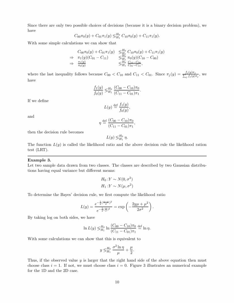
Thus, if the observed value y is larger that the right hand side of the above equation then mustchoose class i = 1. If not, we must choose class i = 0. Figure 3 illustrates an numerical examplefor the 1D and the 2D case.

10

20 21 22 23 24 250.0

0.2

0.4

0.6

0.8

1.0

1.2 Class H1

Class H0

arbi

trary

sca

le

X values

Decision boundary

7.2 7.3 7.4 7.5 7.6 7.7 7.82.30

2.35

2.40

2.45

2.50

2.55

2.60

2.65

2.70

Class H0

Class H1

Y v

alue

s

X values

Decision boundary

Figure 3: Decision boundaries for a binary hypothesis testing problem of 1D and 2D Gaussian.

The above general Bayes decision rule can be simplified when we assume a uniform cost. Inthis case, we have

f1(y)

f0(y)≶H0

H1

π0π1

,

which is equivalent to

π1(y) ≶H0

H1π0(y).

Therefore, we will claim H0 if π0(y) > π1(y) and vice versa. Or equivalently, we have

δ(y) = argmaxi

πi(y).

Since πi(y) is the posterior probability, we can the resulting decision rule as the maximum-a-posteriori decision.

Example 4.

Consider Example 3 with uniform cost. Then, the MAP decision rule is (with η = 1)

y <µ

2.

3.5 M-ary Hypothesis Testing

We can generalize the above binary hypothesis testing problem to a M -ary hypothesis testingproblem. In M-ary hypothesis testing, there are M hypotheses or classes which we wish to assignour observations. The Bayesian decision rule is based again on minimizing the risk similarly to thebinary case:

δB(y) = argmini

M−1∑

j=0

C(i, j)πj(y). (33)

11

By Bayes’ theorem, we have

δB(y) = argmini

M−1∑

j=0

C(i, j)πjfj(y)

f(y).

Now, we can divide the posterior distribution by the posterior of H0 without affecting the minimizerof the optimizaiton:

δB(y) = argmini

M−1∑

j=0

C(i, j)

πjfj(y)f(y)

π0f0(y)f(y)

,

= argmini

M−1∑

j=0

C(i, j)πjfj(y)

π0f0(y).

By defining

Lj(y)def=

fj(y)

f0(y), and hi(y) =

M−1∑

j=0

C(i, j)πjπ0

Lj(y),

we can show thatδB(y) = argmin

ihi(y).

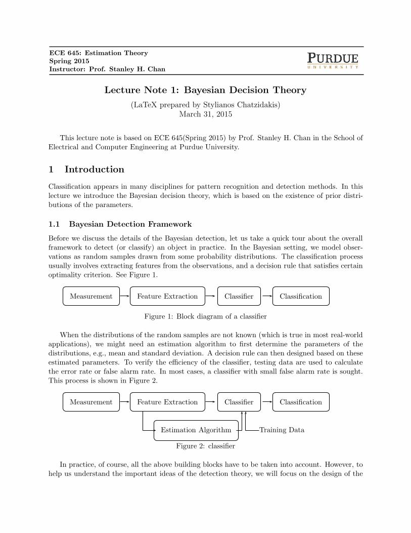
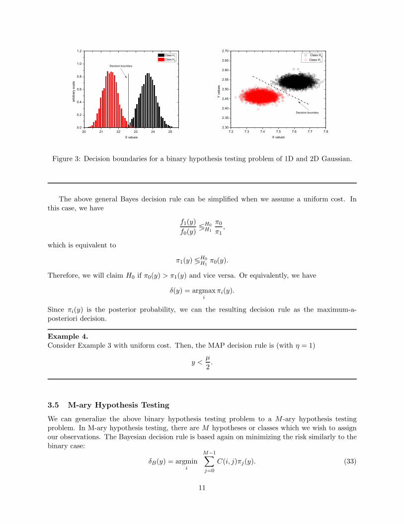
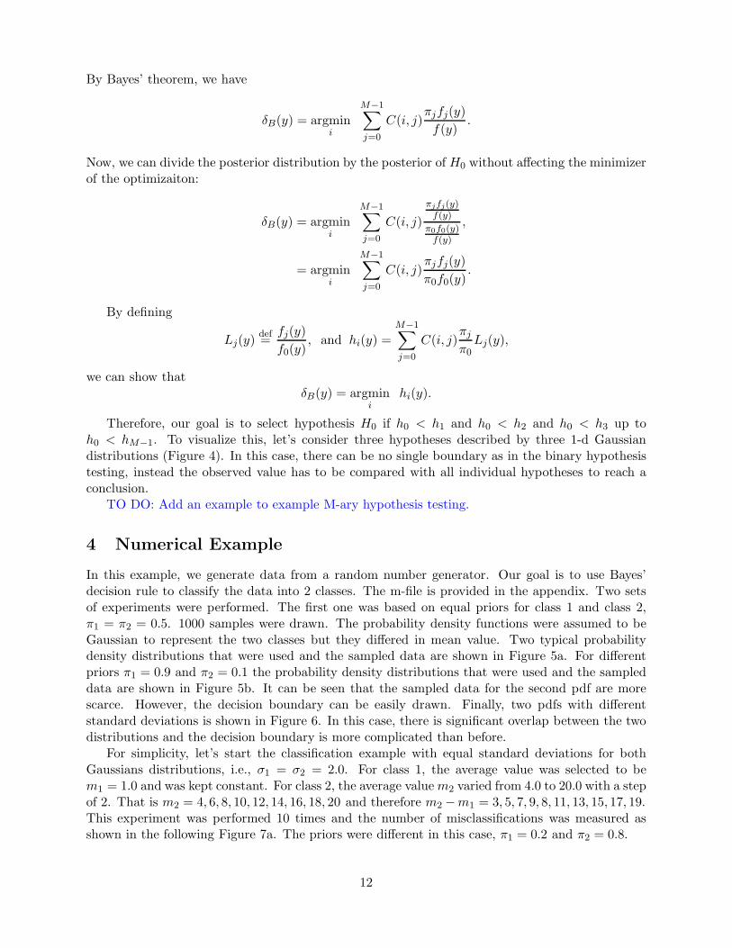
Therefore, our goal is to select hypothesis H0 if h0 < h1 and h0 < h2 and h0 < h3 up toh0 < hM−1. To visualize this, let’s consider three hypotheses described by three 1-d Gaussiandistributions (Figure 4). In this case, there can be no single boundary as in the binary hypothesistesting, instead the observed value has to be compared with all individual hypotheses to reach aconclusion.

TO DO: Add an example to example M-ary hypothesis testing.

4 Numerical Example

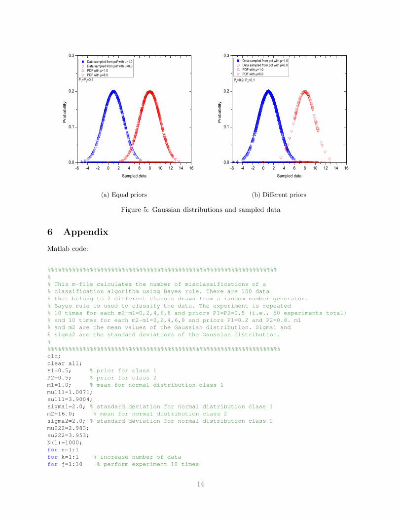
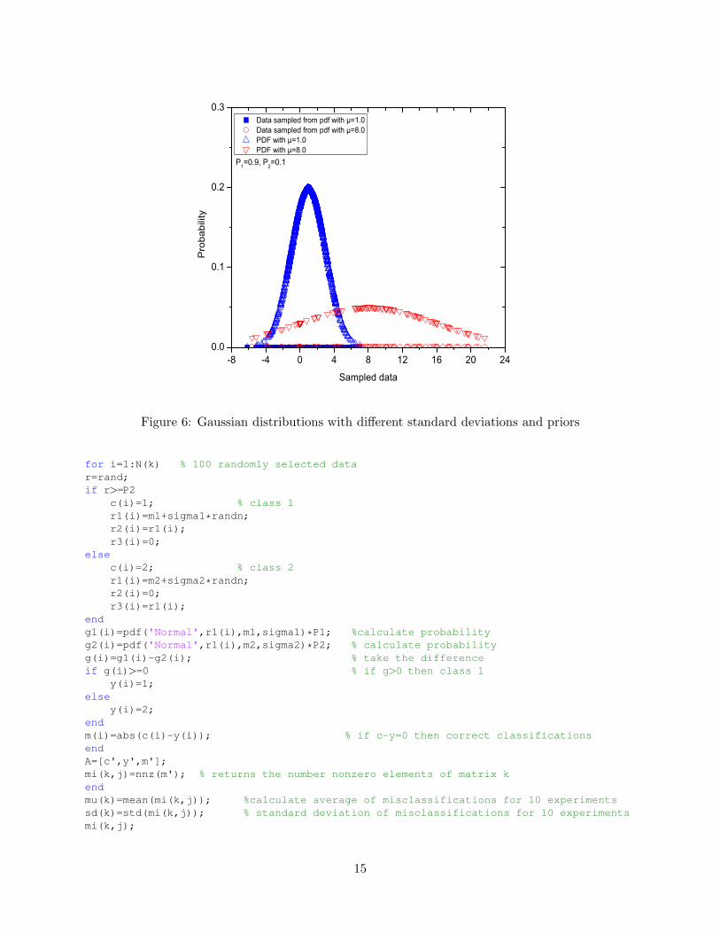
In this example, we generate data from a random number generator. Our goal is to use Bayes’decision rule to classify the data into 2 classes. The m-file is provided in the appendix. Two setsof experiments were performed. The first one was based on equal priors for class 1 and class 2,π1 = π2 = 0.5. 1000 samples were drawn. The probability density functions were assumed to beGaussian to represent the two classes but they differed in mean value. Two typical probabilitydensity distributions that were used and the sampled data are shown in Figure 5a. For differentpriors π1 = 0.9 and π2 = 0.1 the probability density distributions that were used and the sampleddata are shown in Figure 5b. It can be seen that the sampled data for the second pdf are morescarce. However, the decision boundary can be easily drawn. Finally, two pdfs with differentstandard deviations is shown in Figure 6. In this case, there is significant overlap between the twodistributions and the decision boundary is more complicated than before.

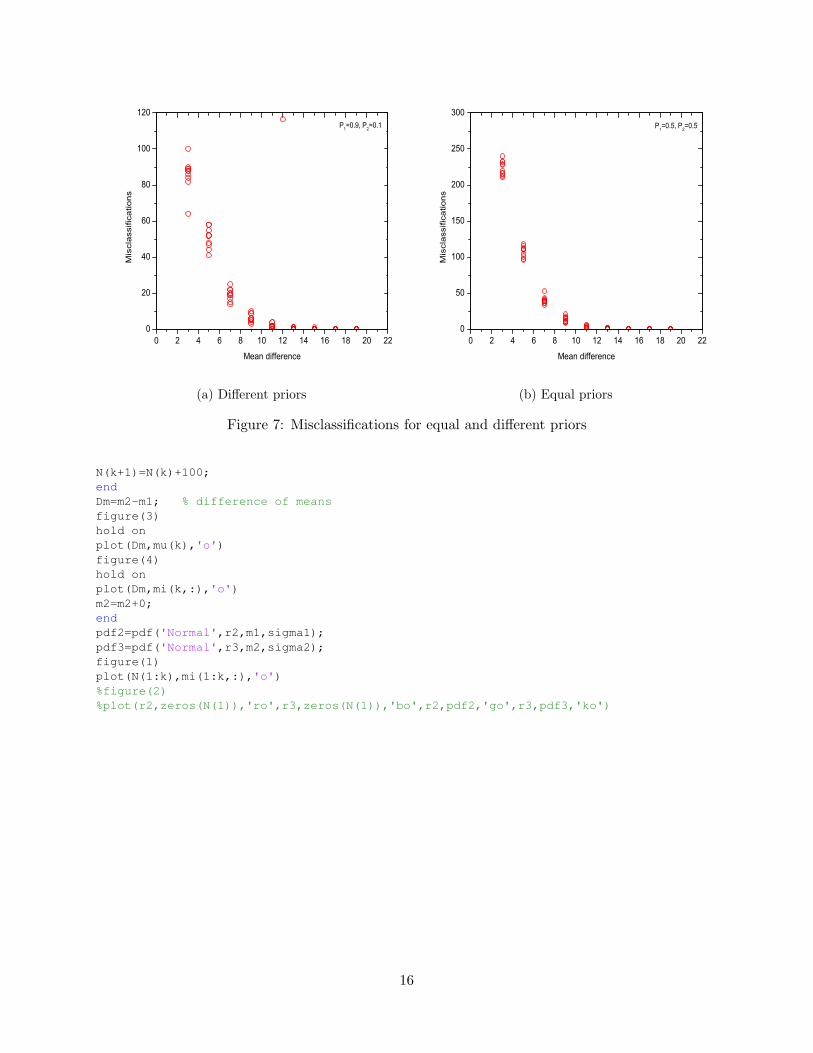
For simplicity, let’s start the classification example with equal standard deviations for bothGaussians distributions, i.e., σ1 = σ2 = 2.0. For class 1, the average value was selected to bem1 = 1.0 and was kept constant. For class 2, the average valuem2 varied from 4.0 to 20.0 with a stepof 2. That is m2 = 4, 6, 8, 10, 12, 14, 16, 18, 20 and therefore m2 −m1 = 3, 5, 7, 9, 8, 11, 13, 15, 17, 19.This experiment was performed 10 times and the number of misclassifications was measured asshown in the following Figure 7a. The priors were different in this case, π1 = 0.2 and π2 = 0.8.

12

6.6 6.8 7.0 7.2 7.4 7.6 7.8 8.00

1

2

3

4

5

6

7

8

arbi

trar

y sc

ale

X values

Class H2

Class H1

Class H0

Figure 4: M=3 hypotheses

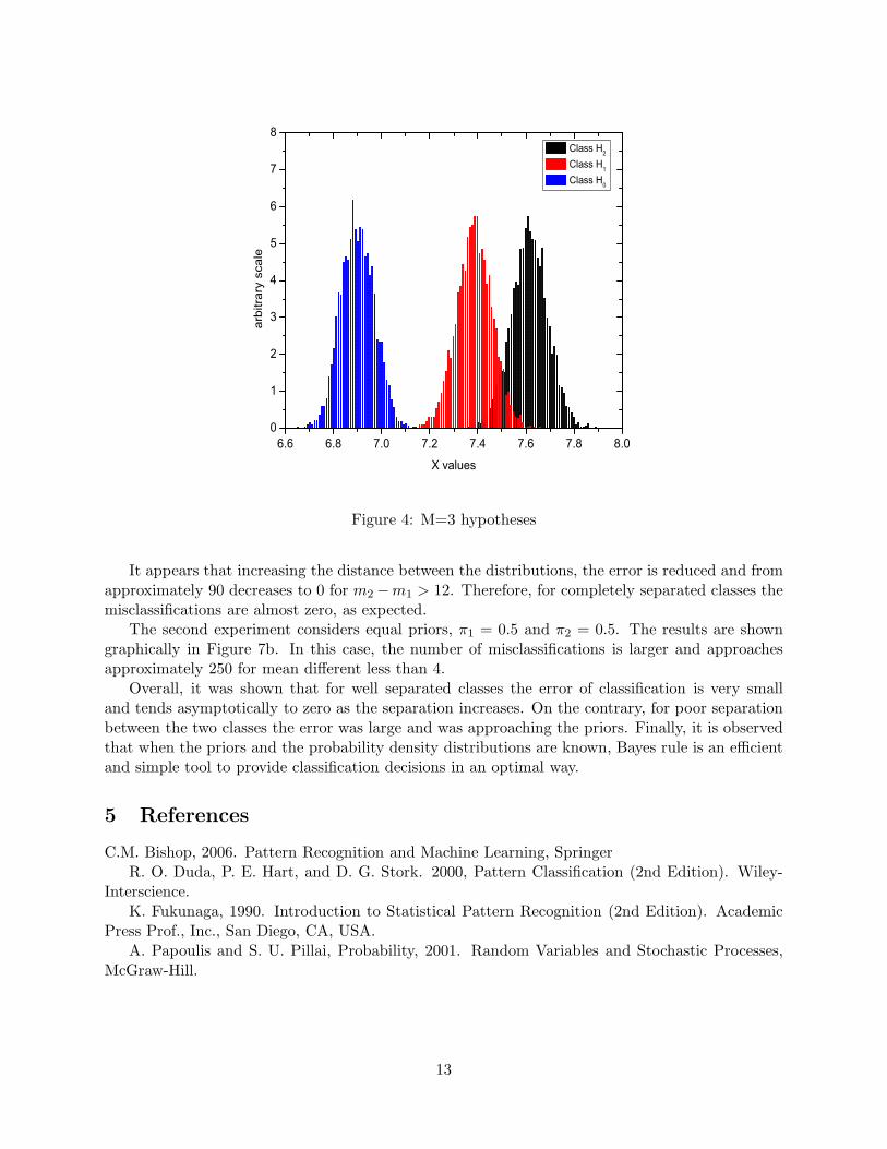
It appears that increasing the distance between the distributions, the error is reduced and fromapproximately 90 decreases to 0 for m2 −m1 > 12. Therefore, for completely separated classes themisclassifications are almost zero, as expected.

The second experiment considers equal priors, π1 = 0.5 and π2 = 0.5. The results are showngraphically in Figure 7b. In this case, the number of misclassifications is larger and approachesapproximately 250 for mean different less than 4.

Overall, it was shown that for well separated classes the error of classification is very smalland tends asymptotically to zero as the separation increases. On the contrary, for poor separationbetween the two classes the error was large and was approaching the priors. Finally, it is observedthat when the priors and the probability density distributions are known, Bayes rule is an efficientand simple tool to provide classification decisions in an optimal way.

5 References

C.M. Bishop, 2006. Pattern Recognition and Machine Learning, SpringerR. O. Duda, P. E. Hart, and D. G. Stork. 2000, Pattern Classification (2nd Edition). Wiley-

Interscience.K. Fukunaga, 1990. Introduction to Statistical Pattern Recognition (2nd Edition). Academic

Press Prof., Inc., San Diego, CA, USA.A. Papoulis and S. U. Pillai, Probability, 2001. Random Variables and Stochastic Processes,

McGraw-Hill.

13

-6 -4 -2 0 2 4 6 8 10 12 14 160.0

0.1

0.2

0.3

Data sampled from pdf with =1.0 Data sampled from pdf with =8.0 PDF with =1.0 PDF with =8.0

Pro

babi

lity

Sampled data

P1=P2=0.5

(a) Equal priors

-6 -4 -2 0 2 4 6 8 10 12 14 160.0

0.1

0.2

0.3

P1=0.9, P2=0.1

Data sampled from pdf with =1.0 Data sampled from pdf with =8.0 PDF with =1.0 PDF with =8.0

Pro

babi

lity

Sampled data

(b) Different priors

Figure 5: Gaussian distributions and sampled data

6 Appendix

Matlab code:

%%%%%%%%%%%%%%%%%%%%%%%%%%%%%%%%%%%%%%%%%%%%%%%%%%%%%%%%%%%%%%%%%

%

% This m-file calculates the number of misclassifications of a

% classification algorithm using Bayes rule. There are 100 data

% that belong to 2 different classes drawn from a random number generator.

% Bayes rule is used to classify the data. The experiment is repeated

% 10 times for each m2-m1=0,2,4,6,8 and priors P1=P2=0.5 (i.e., 50 experiments total)

% and 10 times for each m2-m1=0,2,4,6,8 and priors P1=0.2 and P2=0.8. m1

% and m2 are the mean values of the Gaussian distribution. Sigma1 and

% sigma2 are the standard deviations of the Gaussian distribution.

%

%%%%%%%%%%%%%%%%%%%%%%%%%%%%%%%%%%%%%%%%%%%%%%%%%%%%%%%%%%%%%%%%%%

clc;

clear all;

P1=0.5; % prior for class 1

P2=0.5; % prior for class 2

m1=1.0; % mean for normal distribution class 1

mu111=1.0071;

su111=3.9004;

sigma1=2.0; % standard deviation for normal distribution class 1

m2=16.0; % mean for normal distribution class 2

sigma2=2.0; % standard deviation for normal distribution class 2

mu222=2.983;

su222=3.953;

N(1)=1000;

for n=1:1

for k=1:1 % increase number of data

for j=1:10 % perform experiment 10 times

14

-8 -4 0 4 8 12 16 20 240.0

0.1

0.2

0.3

P1=0.9, P2=0.1

Data sampled from pdf with =1.0 Data sampled from pdf with =8.0 PDF with =1.0 PDF with =8.0

Pro

babi

lity

Sampled data

Figure 6: Gaussian distributions with different standard deviations and priors

for i=1:N(k) % 100 randomly selected data

r=rand;

if r>=P2

c(i)=1; % class 1

r1(i)=m1+sigma1*randn;

r2(i)=r1(i);

r3(i)=0;

else

c(i)=2; % class 2

r1(i)=m2+sigma2*randn;

r2(i)=0;

r3(i)=r1(i);

end

g1(i)=pdf('Normal',r1(i),m1,sigma1)*P1; %calculate probability

g2(i)=pdf('Normal',r1(i),m2,sigma2)*P2; % calculate probability

g(i)=g1(i)-g2(i); % take the difference

if g(i)>=0 % if g>0 then class 1

y(i)=1;

else

y(i)=2;

end

m(i)=abs(c(i)-y(i)); % if c-y=0 then correct classifications

end

A=[c',y',m'];

mi(k,j)=nnz(m'); % returns the number nonzero elements of matrix k

end

mu(k)=mean(mi(k,j)); %calculate average of misclassifications for 10 experiments

sd(k)=std(mi(k,j)); % standard deviation of misclassifications for 10 experiments

mi(k,j);

15

0 2 4 6 8 10 12 14 16 18 20 220

20

40

60

80

100

120P1=0.9, P2=0.1

Mis

clas

sific

atio

ns

Mean difference

(a) Different priors

0 2 4 6 8 10 12 14 16 18 20 220

50

100

150

200

250

300P1=0.5, P2=0.5

Mis

clas

sific

atio

ns

Mean difference

(b) Equal priors

Figure 7: Misclassifications for equal and different priors

N(k+1)=N(k)+100;

end

Dm=m2-m1; % difference of means

figure(3)

hold on

plot(Dm,mu(k),'o')

figure(4)

hold on

plot(Dm,mi(k,:),'o')

m2=m2+0;

end

pdf2=pdf('Normal',r2,m1,sigma1);

pdf3=pdf('Normal',r3,m2,sigma2);

figure(1)

plot(N(1:k),mi(1:k,:),'o')

%figure(2)

%plot(r2,zeros(N(1)),'ro',r3,zeros(N(1)),'bo',r2,pdf2,'go',r3,pdf3,'ko')

16