DETECTION, DECISIONS, AND HYPOTHESIS TESTING · Chapter 8 DETECTION, DECISIONS, AND HYPOTHESIS TESTING Detection, decision making, and hypothesis testing are di↵erent names for

Chapter 8

DETECTION, DECISIONS, ANDHYPOTHESIS TESTING

Detection, decision making, and hypothesis testing are di↵erent names for the same proce-dure. The word detection refers to the e↵ort to decide whether some phenomenon is presentor not in a given situation. For example, a radar system attempts to detect whether or nota target is present; a quality control system attempts to detect whether a unit is defective;a medical test detects whether a given disease is present. The meaning has been extendedin the communication field to detect which one, among a finite set of mutually exclusivepossible transmited signals, has been transmitted. Decision making is, again, the processof choosing between a number of mutually exclusive alternatives. Hypothesis testing is thesame, except the mutually exclusive alternatives are called hypotheses. We usually use theword hypotheses for these alternatives in what follows, since the word seems to conjure upthe appropriate intuitive images.

These problems will usually be modeled by a generic type of probability model. Each suchmodel is characterized by a discrete random variable (rv) X called the hypothesis rv andanother rv or random vector Y called the observation rv. The sample values of X are calledhypotheses; it makes no di↵erence what these hypotheses are called, so we usually numberthem, 0, 1, . . . ,M � 1. When the experiment is performed, the resulting sample point !maps into a sample value x for X, x 2 {0, 1,M�1}, and into a sample value y for Y. Thedecision maker observes y (but not x) and maps y into a decision x̂(y). The decision iscorrect if x̂(y) = x.

The probability px = pX (x) of hypothesis x is referred to as the a priori probability ofhypothesis x. The probability model is completed by the conditional distribution of Y,conditional on each sample value of X. These conditional distributions are called likelihoodsin the terminology of hypothesis testing. In most of the situations we consider, theseconditional distributions are represented either by a PMF or by joint probability densitiesover Rn for a given n � 1. To avoid repeating everything, probability densities are usuallyassumed. Arguments that cannot be converted to discrete observations simply by replacingPDF’s with PMF’s and changing integrals to sums will be discussed as they arise. There arealso occasional comments about observations that cannot be described by PDF’s or PMF’s.

391

392 CHAPTER 8. DETECTION, DECISIONS, AND HYPOTHESIS TESTING

As with any probability model representing a real-world phenomenon, the random variablesmight model quantities that are actually random, or quantities such as coin tosses that mightbe viewed as either random or deterministic, or quantities such as physical constants thatare deterministic but unknown. In addition, the model might be chosen for its simplicity,or for its similarity to some better-understood phenomenon, or for its faithfulness to someaspect of the real-world phenomenon.

Classical statisticians1 are uncomfortable with the use of completely probabilistic models tostudy hypothesis testing, particularly when the ‘correct’ hypothesis is not obviously randomwith known probabilities. They have no objection to a separate probability model for theobservation under each hypothesis, but are unwilling to choose a priori probabilities forthe hypotheses. This is partly a practical matter, since statisticians design experimentsto gather data and make decisions that often have considerable political and commercialimportance. The use of a priori probabilities could be viewed as biasing these decisions andthus losing the appearance of impartiality.

The approach in this text, as pointed out frequently before, is to use a variety of probabilitymodels to gain insight and understanding about real-world phenomena. If we assume avariety of a priori probabilities and then see how the results depend on those choices, weoften learn more than if we refuse to consider a priori probabilities at all. Another verysimilar approach that we often use is to consider a complete probabilistic model, but toassume that the observer does not know the a priori probabilities and makes a decision notbased on them.2 This is illustrated in the development of the Neyman-Pearson criterion inSection 8.4.

Before discussing how to make decisions, it is important to understand when and whydecisions must be made. As an example, suppose we conclude, on the basis of an observation,that hypothesis 0 is correct with probability 2/3 and hypothesis 1 with probability 1/3.Simply making a decision on hypothesis 0 and forgetting about the probabilities throwsaway much of the information that has been gathered. The issue, however, is that sometimeschoices must be made. In a communication system, the recipient wants to receive themessage (perhaps with an occasional error) rather than a set of probabilities. In a controlsystem, the controls must occasionally take action. Similarly managers must occasionallychoose between courses of action, between products, and between people to hire. In a sense,it is by making decisions (and, in Chapter 10, by making estimates) that we return fromthe world of mathematical probability models to the world being modeled.

8.1 Decision criteria and the MAP criterion

There are a number of possible criteria for making decisions, and initially we concentrateon maximizing the probability of making correct decisions. For each hypothesis x, let px

1Statisticians have argued since the time of Bayes about the ‘validity’ of choosing a priori probabilitiesfor hypotheses to be tested. Bayesian statisticians are comfortable with this practice and non-Bayesian orclassical statisticians are not.

2Note that any decision procedure not using a priori probabilities can be made whether one believes thea priori probabilities exist but are unknown or do not exist at all.

8.1. DECISION CRITERIA AND THE MAP CRITERION 393

be the a priori probability that X = x and let fY |X (y | x) be the joint probability density

(called a likelihood) that Y = y conditional on X = x. If fY (y) > 0, then the probabilitythat X = x, conditional on Y = y , is given by Bayes’ law as

pX|Y (x | y) =

pxfY |X (y | x)fY (y)

where fY (y) =M�1Xx=0

pxfY |X (y | x). (8.1)

Whether Y is discrete or continuous, the set of sample values where fY (y) = 0 or pY (y) = 0is an event of zero probability. Thus we ignore this event in what follows and simply assumethat fY (y) > 0 or pY (y) > 0 for all sample values.

The decision maker observes y and must choose one hypothesis, say x̂(y), from the set ofpossible hypotheses. The probability that hypothesis x is correct (i.e., the probability thatX = x) conditional on observation y is given in (8.1). Thus, in order to maximize theprobability of choosing correctly, the observer should choose that x for which p

X|Y (x | y)is maximized. Writing this as an equation,

x̂(y) = arg maxx

⇥p

X|Y (x | y)⇤

(MAP rule). (8.2)

where arg maxx means the argument x 2 {0, . . . ,M�1} that maximizes the function. Theconditional probability p

X|Y (x | y) is called an a posteriori probability, and thus the decisionrule in (8.2) is called a maximum a posteriori probability (MAP) rule. Since we want todiscuss other rules as well, we often denote the x̂(y) given in (8.2) as x̂MAP(y).

An equivalent representation of (8.2) is obtained by substituting (8.1) into (8.2) and ob-serving that fY (y) is the same for all hypotheses. Thus,

x̂MAP(y) = arg maxx

⇥pxf

Y |X (y | x)⇤. (8.3)

It is possible for the maximum in (8.3) to be achieved by several hypotheses. Each suchhypothesis will maximize the probability of correct decision, but there is a need for a tie-breaking rule to actually make a decision. Ties could be broken in a random way (and thisis essentially necessary in Section 8.4), but then the decision is more than a function of theobservation. In many situations, it is useful for decisions to be (deterministic) functions ofthe observations.

Definition 8.1.1. A test is a decision x̂(y) that is a (deterministic) function of the obser-vation.

In order to fully define the MAP rule in (8.3) as a test, we arbitrarily choose the largestmaximizing x. An arbitrary test A, i.e., an arbitrary deterministic rule for choosing anhypothesis from an observation y , can be viewed as a function, say x̂A(y), mapping the setof observations to the set of hypotheses, {0, 1, . . . ,M�1}. For any test A, then, p

X|Y (x̂A | y)is the probability that x̂A(y) is the correct decision when test A is used on observation y .Since xMAP(y) maximizes the probability of correct decision, we have

pX|Y

�x̂MAP(y) | y

�� p

X|Y

�x̂A(y) | y

�; for all A and y . (8.4)


For simplicity of notation, we assume in what follows that the observation Y , conditionalon each hypothesis, has a joint probability density. Then Y also has a marginal densityfY (y). Averaging (8.4) over observations,

ZfY (y)p

X|Y

�x̂MAP(y) |y

�dy �

ZfY (y)p

X|Y

�x̂A(y) |y

�dy . (8.5)

The quantity on the left is the overall probability of correct decision using x̂MAP , and thaton the right is the overall probability of correct decision using x̂A . The above results arevery simple, but also important and fundamental. We summarize them in the followingtheorem, which applies equally for observations with a PDF or PMF.

Theorem 8.1.1. Assume that Y has a joint PDF or PMF conditional on each hypothe-sis. The MAP rule, given in (8.2) (or equivalently in (8.3)), maximizes the probability ofcorrect decision conditional on each observed sample value y. It also maximizes the overallprobability of correct decision given in (8.5).

Proof:3 The only questionable issue about the theorem is whether the integrals in (8.5)exist whenever Y has a density. Using (8.1), the integrands in (8.5) can be rewritten as

Zpx̂MAP(y)fY |X

�y | x̂MAP(y)

�dy �

Zpx̂A(y)fY |X

�y | x̂A(y)

�dy . (8.6)

The right hand integrand of (8.6) can be expressed in a less obscure way by noting thatthe function x̂A(y) is specified by defining, for each hypothesis `, the set A` of observationsy 2 Rn for which x̂A(y) = `, i.e., A` = {y : x̂A(y) = `}. Using these sets, the integral onthe right is given byZ

px̂A(y)fY |X

�y | x̂A(y)

�dy =

X`

p`

Zy2A`

fY |X (y | `) dy

=X

`

p` Pr{A` | X = `} (8.7)

=X

`

p` PrnX̂A = ` | X = `

o, (8.8)

where X̂A = x̂A(Y ). The integral above exists if the likelihoods are measurable func-tions and if the sets A` are measurable sets. This is virtually no restriction and is hence-forth assumed without further question. The integral on the left side of (8.6) is simi-larly

P` p`Pr

nX̂MAP = ` | X = `

o, which exists if the likelihoods are measurable functions.

Before discussing the implications and use of the MAP rule, we review the assumptions thathave been made. First, we assumed a probability experiment in which all probabilities areknown, and in which, for each performance of the experiment, one and only one hypothesis is

3This proof deals with mathematical details and involves both elementary notions of measure theory andconceptual di�culty; readers may safely omit it or postpone the proof until learning measure theory.

8.2. BINARY MAP DETECTION 395

correct. This conforms very well to a communication model in which a transmitter sends oneof a set of possible signals, and the receiver, given signal plus noise, makes a decision on thetransmitted signal. It does not always conform well to a scientific experiment attempting toverify the existence of some new phenomenon; in such situations, there is often no sensibleway to model a priori probabilities. In section 8.4, we find ways to avoid depending on apriori probabilities.

The next assumption was that maximizing the probability of correct decision is an appropri-ate decision criterion. In many situations, the cost of right and wrong decisions are highlyasymmetric. For example, when testing for a treatable but deadly disease, making an errorwhen the disease is present is far more dangerous than making an error when the disease isnot present. In Section 8.3 we define a minimum-cost formulation which allows us to treatthese asymmetric cases.

The MAP rule can be extended to broader assumptions than the existence of a PMF orPDF. This is carried out in Exercise 8.12 but requires a slight generalization of the notionof a MAP rule at each sample observation y .

In the next three sections, we restrict attention to the case of binary hypotheses. Thisallows us to understand most of the important ideas but simplifies the notation and detailsconsiderably. In Section 8.5, we again consider an arbitrary number of hypotheses.

8.2 Binary MAP detection

Assume a probability model in which the hypothesis rv X is binary with pX (0) = p0 > 0 andpX (1) = p1 > 0. Let Y be an n-rv Y = (Y1, . . . , Yn)T whose conditional probability density,fY |X (y | `), is initially assumed to be finite and non-zero for all y 2 Rn and ` 2 {0, 1}. Themarginal density of Y is given by fY (y) = p0fY |X (y | 0)+p1fY |X (y | 1) > 0. The a posterioriprobability of X = 0 or X = 1, is given by

pX|Y (x | y) =p`fY |X (y | x)

fY (y). (8.9)

Writing out (8.2) explicitly for this case,

p1fY |X (y | 1)fY (y)

x̂(y)=1�<

x̂(y)=0

p0fY |X (y | 0)fY (y)

. (8.10)

This “equation” indicates that the decision is 1 if the left side is greater than or equal tothe right, and is 0 if the left side is less than the right. Choosing the decision to be 1 whenequality holds is arbitrary and does not a↵ect the probability of being correct. CancelingfY (y) and rearranging,

⇤(y) =fY |X (y | 1)fY |X (y | 0)

x̂(y)=1�<

x̂(y)=0

p0

p1= ⌘. (8.11)


The ratio ⇤(y) = pY |X (y | 1)/p

Y |X (y | 0) is called the likelihood ratio for a binary decisionproblem. It is a function only of y and not the a priori probabilities.4 The detection rulein (8.11) is called a threshold rule and its right side, ⌘ = p0/p1 is called the threshold, whichin this case is a function only of the a priori probabilities.

Note that if the a priori probability p0 is increased in (8.11), then the threshold in-creases, and the set of y for which hypothesis 0 is chosen increases; this corresponds to ourintuition—the greater our initial comviction that X is 0, the stronger the evidence requiredto change our minds.

Next consider a slightly more general binary case in which fY |X (y | `) might be 0 (although,

as discussed before fY (y) > 0 and thus at least one of the likelihoods must be positive foreach y). In this case, the likelihood ratio can be either 0 or 1 depending on which of thetwo likelihoods is 0. This more general case does not require any special care except for thedevelopment of the error curve in Section 8.4. Thus we include this generalization in whatfollows.

We will look later at a number of other detection rules, including maximum likelihood,minimum-cost, and Neyman-Pearson. These are also essentially threshold rules that di↵erfrom the MAP test in the choice of the threshold ⌘ (and perhaps in the tie-breaking rulewhen the likelihood ratio equals the threshold). In general, a binary threshold rule isa decision rule between two hypotheses in which the likelihood ratio is compared to athreshold, where the threshold is a real number not dependent on the observation. Asdiscussed in Section 8.3, there are also situations for which threshold rules are inappropriate.

An important special case of (8.11) is that in which p0 = p1. In this case ⌘ = 1. The rule isthen x̂(y) = 1 for y such that p

Y |X (y | 1) � pY |X (y | 0) (and x̂(y) = 0 otherwise). This is

called a maximum likelihood (ML) rule or test. The maximum likelihood test is often usedwhen p0 and p1 are unknown, as discussed later.

We now find the probability of error, Pr{e⌘ | X=x}, under each hypothesis5 x using athreshold at ⌘ From this we can also find the overall probability of error, Pr{e⌘} =p0Pr{e⌘ | X=0}+ p1Pr{e⌘ | X=1} where ⌘ = p0/p1.

Note that (8.11) partitions the space of observed sample values into 2 regions. The regionA = {y : ⇤(y) � ⌘} specifies where x̂ = 1 and the region Ac = {y : ⇤(y) < ⌘} specifieswhere x̂ = 0. For X=0, an error occurs if and only if y is in Ac; for X = 1, an error occursif and only if y is in A. Thus,

Pr{e⌘ | X=0} =Zy✏A1

fY |X (y | 0) dy . (8.12)

4For non-Bayesians, the likelihood ratio is one rv in the model for X = 0 and another rv in the modelfor X = 1, but is not a rv overall.

5In the radar field, Pr{e | X=0} is called the probability of false alarm, and Pr{e | X=1} (for any giventest) is called the probability of a miss. Also 1 � Pr{e | X=1} is called the probability of detection. Instatistics, Pr{e | X=1} is called the probability of error of the second kind, and Pr{e | X=0} is the probabilityof error of the first kind. I feel that all this terminology conceals the fundamental symmetry between thetwo hypotheses. The names 0 and 1 of the hypotheses could be interchanged, or they could be renamed, forexample, as Alice and Bob or Apollo and Zeus, with only minor complications in notation.


Pr{e⌘ | X=1} =Zy✏A0

fY |X (y | 1) dy . (8.13)

In several of the examples to follow, the error probability can be evaluated in a simplerway by working directly with the likelihood ratio. Since ⇤(y) is a function of the observedsample value y , we can define the likelihood ratio random variable ⇤(Y ) in the usual way,i.e., for every sample point !, Y (!) is the sample value for Y , and ⇤(Y (!)) is the samplevalue of ⇤(Y ). In the same way, x̂(Y (!)) (or more briefly X̂) is the decision randomvariable. In these terms, (8.11) states that

X̂ = 1 if and only if ⇤(Y ) � ⌘. (8.14)

Thus,

Pr{e⌘ | X=0} = PrnX̂=1 | X=0

o= Pr{⇤(Y ) � ⌘ | X=0} . (8.15)

Pr{e⌘ | X=1} = PrnX̂=0 | X=1

o= Pr{⇤(Y ) < ⌘ | X=1} . (8.16)

This means that if the one-dimensional quantity ⇤(y) can be found easily from the obser-vation y , then it can be used, with no further reference to y , both to perform any thresholdtest and to find the resulting error probability.

8.2.1 Su�cient statistics I

The previous section suggests that binary hypothesis testing can often be separated into twoparts, first finding the likelihood ratio for a given observation, and then doing everythingelse on the basis of the likelihood ratio. Sometimes it is simpler to find a quantity that isa one-to-one function of the likelihood ratio (the log of the likelihood ratio is a commonchoice) and sometimes it is simpler to calculate some intermediate quantity from which thelikelihood ratio can be found. Both of these are called su�cient statistics, as defined moreprecisely below.

Definition 8.2.1 (Su�cient statistics for binary hypotheses). For binary hypothesistesting, a su�cient statistic is any function v(y) of the observation y from which the likeli-hood ratio can be calculated, i.e., v(y) is a su�cient statistic if a function u(v) exists suchthat ⇤(y) = u(v(y)) for all y.

For example, y itself, ⇤(y), and any one to one function of ⇤(y) are su�cient statis-tics. For vector or process observations in particular, ⇤(Y ) (or any one-to-one function of⇤(Y )) is often simpler to work with than Y itself, since ⇤(Y ) is one dimensional ratherthan many dimensional. As indicated by these examples, v(y) can be one dimensional ormultidimensional.

An important example of a su�cient statistic is the log-likelihood ratio, LLR(Y ) = ln[⇤(Y )].We will often find that the LLR is more convenient to work with than ⇤(Y ). We next lookat some widely used examples of binary MAP detection where the LLR and other su�cientstatistics are useful. We will then develop additional properties of su�cient statistics.


8.2.2 Binary detection with a one-dimensional observation

Example 8.2.1 (Detection of antipodal signals in Gaussian noise). First we look ata simple abstraction of a common digital communication system in which a single binarydigit is transmitted and that digit plus Gaussian noise is received. The observation is thentaken to be Y = X + Z, where Z ⇠ N (0,�2) is Gaussian and X (the transmitted rv andthe hypothesis) is binary and independent of Z. It is convenient to relabel hypothesis 1 asb and hypothesis 0 as �b.

The receiver must detect, from the observed sample value y of Y , whether the sample valueof X is �b or b.

We will see in subsequent examples that the approach here can be used if the binaryhypothesis is a choice between two vectors in the presence of a Gaussian vector or a choicebetween two waveforms in the presence of a Gaussian process. In fact, not only can thesame approach be used, but the problem essentially reduces to the single dimensional casehere.

Conditional on X = b, the observation is Y ⇠ N (b,�2) and, conditional on X = �b,Y ⇠ N (�b,�2), i.e.,

fY |X (y | b) =

1p2⇡�2

exp�(y � b)2

(2�2)

�; f

Y |X (y | �b) =1p

2⇡�2exp

�(y + b)2

(2�2)

�.

The likelihood ratio is the ratio of f(y | b) to f(y | �b), given by

⇤(y) = exp(y + b)2 � (y � b)2

2�2

�= exp

2yb

�2

�. (8.17)

Substituting this into (8.11), with p0 = pX (�b) and p1 = pX (b),

⇤(y) = exp2yb

�2

� x̂(y)=b�<

x̂(y)=�b

p0

p1= ⌘. (8.18)

This is further simplified by taking the logarithm, yielding

LLR(y) =2yb

�2

� x̂(y)=b�<

x̂(y)=�b

ln ⌘. (8.19)

This can be rewritten as a threshold rule on y directly,

y

x̂(y)=b�<

x̂(y)=�b

�2 ln ⌘

2b. (8.20)

In the maximum likelihood (ML) case (p1 = p0), the threshold ⌘ is 1, so ln ⌘ = 0. Thus, asillustrated in Figure 8.1, the ML rule maps y � 0 into x̂ = b and y < 0 into x̂ = �b.


0PP⇠⇠⇠⇠⇠⇠⇠⇠⇠⇠⇠⇠XXXXX XXX XXX

@@I�b b

v

fY |X (y | b)f

Y |X (y | �b)

Pr�e��X = �b

x̂=b-

x̂=�b�

Figure 8.1: Binary hypothesis testing for antipodal signals, �b and +b with ⌘ = 1.The figure also illustrates the error probability given X = �b and using maximumlikelihood detection (⌘ = 1). If one visualizes shifting the threshold away from 0, it isnot surprising geometrically that the MAP threshold for ⌘ = 1 is at 0.

Still assuming maximum likelihood, an error occurs, conditional on X = �b, if Y � 0. Thisis the same as the probability that the normalized Gaussian rv (Y + b)/� exceeds b/�. Thisin turn is Q(b/�) where Q(u) is the complementary CDF of a normalized Gaussian rv,

Q(u) =Z 1

u

12⇡

exp��z2

2�dz. (8.21)

It is easy to see (especially with the help of Figure 8.1) that with maximum likelihood, theprobability of error conditional on X = b is the same, so

Pr�e��X = b

= Pr

�e��X = �b

= Pr{e} = Q(b/�). (8.22)

It can be seen that with maximum likelihood detection, the error probability depends onlyon the ratio b/�, which we denote as �. The reason for this dependence on � alone canbe seen by dimensional analysis. That is, if the signal amplitude and the noise standarddeviation are measured in a di↵erent system of units, the error probability would not change.We view �2 as a signal to noise ratio, i.e., the signal value squared (which can be interpretedas signal energy) divided by �2 which can be interpreted in this context as noise energy.

It is now time to look at what happens when ⌘ = p0/p1 is not 1. Using (8.20) to find theerror probability as before, and using � = b/�,

Pr�e⌘

��X = �b

= Q

✓� +

ln ⌘

2�

◆(8.23)

Pr�e⌘

��X = b

= Q

✓� � ln ⌘

2�

◆. (8.24)

If ln ⌘ > 0, i.e., if p0 > p1, then, for example, if y = 0, the observation alone would provideno evidence whether X = 0 or X = b, but we would choose x̂(y) = �b since it is morelikely a priori. This gives an intuitive explanation why the threshold is moved to the rightif ln ⌘ > 0 and to the left if ln ⌘ < 0.


Example 8.2.2 (Binary detection with a Gaussian noise rv). This is a very smallgeneraliization of the previous example. The binary rv X, instead of being antipodal (i.e.,X = ±b) is now arbitrary, taking on either the arbitrary value a or b where b > a. The apriori probabilities are denoted by p0 and p1 respectively. As before, the observation (atthe receiver) is Y = X + Z where Z ⇠ N (0,�2) and X and Z are independent.

Conditional on X = b, Y ⇠ N (b,�2) and, conditional on X = a, Y ⇠ N (a,�2).

fY |X (y | b) =

1p2⇡�2

exp�(y � b)2

2�2

�; f

Y |X (y | a) =1p

2⇡�2exp

�(y � a)2

2�2

�.

The likelihood ratio is then

⇤(y) = exp(y � a)2 � (y � b)2

2�2

�= exp

2(b� a)y + (a2 � b2)

2�2

�

= exp✓

b� a

�2

◆✓y � b + a

2

◆�. (8.25)

Substituting this into (8.11), we have

exp✓

b� a

�2

◆✓y � b + a

2

◆� x̂(y)=b�<

x̂(y)=a

p0

p1= ⌘. (8.26)

This is further simplified by taking the logarithm, yielding

LLR(y) =✓

b� a

�2

◆✓y � b + a

2

◆� x̂(y)=b�<

x̂(y)=a

ln(⌘). (8.27)

Solving for y, (8.27) can be rewritten as a threshold rule on y directly,

y

x̂(y)=b�<

x̂(y)=a

�2 ln ⌘

b� a+

b + a

2.

This says that the MAP rule simply compares y to a threshold �2 ln ⌘/(b� a) + (b + a)/2.Denoting this threshold for Y as ✓, the MAP rule is

y

x̂(y)=b�<

x̂(y)=a

✓; where ✓ =�2 ln ⌘

b� a+

b + a

2. (8.28)

In the maximum likelihood (ML) case (p1 = p0), the threshold ⌘ for ⇤ is 1 and the threshold✓ for y is the midpoint6 between a and b (i.e., ✓ = (b + a)/2). For the MAP case, If ⌘ islarger or smaller than 1, ✓ is respectively larger or smaller than (b + a)/2 (see Figure 8.2).

6At this point, we see that this example is really the same as Example 8.2.1 with a simple linear shift ofX and Y . Thus this example is redundant, but all these equations might be helpful to make this clear.


cc = (a + b)/2

✓⇠⇠⇠⇠XXXXX X

@@Ia b

v

fY |X (y|b)f

Y |X (y|a)

Pr�e⌘

��X = a

x̂=b-x̂=a

�

Figure 8.2: Binary hypothesis testing for arbitrary signals, a, b, for b > a. This isessentially the same as Figure 8.1 except the midpoint has been shifted to (a+ b)/2 andthe threshold ⌘ is greater than 1 (see (8.28)).

From (8.28), Pr{e⌘ | X=a} = Pr{Y � ✓ | X=a}. Given X = a, Y ⇠ N (a,�2), so, givenX = a, (Y � a)/� is a normalized Gaussian variable.

Pr{Y � ✓ | X=a} = Pr⇢

Y � a

�� ✓ � a

�| X =a

�= Q

✓✓ � a

�

◆. (8.29)

Replacing ✓ in (8.29) by its value in (8.28),

Pr{e⌘ | X=a} = Q

✓� ln ⌘

b� a+

b� a

2�

◆. (8.30)

We evaluate Pr{e⌘ | X=b} = Pr{Y < ✓ | X=b} in the same way. Given X = b, Y isN (b,�2), so

Pr{Y < ✓ | X=b} = Pr⇢

Y � b

�<

✓ � b

�| X =b

�= 1�Q

✓✓ � b

�

◆.

Using (8.28) for ✓ and noting that Q(x) = 1�Q(�x) for any x,

Pr{e⌘ | X=b} = Q

✓�� ln ⌘

b� a+

b� a

2�

◆. (8.31)

Note that (8.30) and (8.31) are functions only of (b�a)/� and ⌘. That is, only the distancebetween b and a is relevant, rather than their individual values, and it is only this distancerelative to � that is relevant. This should be intuitively clear from Figure 8.2. If we define� = (b� a)/(2�), then (8.30) and (8.31) simplify to

Pr{e⌘ | X=a} = Q

✓ln ⌘

2�+ �

◆Pr{e⌘ | X=b} = Q

✓� ln ⌘

2�+ �

◆. (8.32)

For ML detection, ⌘ = 1, and this simplifies further to

Pr{e | X=a} = Pr{e | X=b} = Pr{e} = Q(�). (8.33)

As expected, the solution here is essentially the same as the antipodal case of the previousexample. The only di↵erence is that in the first example, the midpoint between the signalsis 0 and in the present case it is arbitrary. Since this arbitrary o↵set is known at the receiver,it has nothing to do with the error probability. We still interpret �2 as a signal to noiseratio, but the energy in the o↵set is wasted (for the purpose of detection).


8.2.3 Binary MAP detection with vector observations

In this section, we consider the same basic problem as in the last section, except that herethe observation consists of the sample values of n rv’s instead of 1. There is a binaryhypothesis with a priori probabilities pX (0) = p0 > 0 and pX(1) = p1 > 0. There are nobservation rv’s which we view as an n-rv Y = (Y1, . . . , Yn)T. Given a sample value y ofY , we use the maximum a posteriori (MAP) rule to select the most probable hypothesisconditional on y .

It is important to understand that the sample point ! resulting from an experiment leadsto a sample value X(!) for X and sample values Y1(!), . . . , Yn(!) for Y1, . . . , Yn. Whentesting an hypothesis, one often performs many sub-experiments, corresponding to themultiple observations y1, . . . , yn. However, the sample value of the hypothesis (which is notobserved) is constant over these sub-experiments.

The analysis of this n-rv observation is virtually identical to that for a single observationrv (except for the examples which are based explicitly on particular probability densities.)Throughout this section, we assume that the conditional joint distribution of Y conditionalon either hypothesis has a density fY |X(y |`) that is positive over Rn. Then, exactly as inSection 8.2.2,

⇤(y) =fY |X (y | 1)fY |X (y | 0)

x̂(y)=1�<

x̂(y)=0

p0

p1= ⌘. (8.34)

Here ⇤(y) is the likelihood ratio for the observed sample value y . MAP detection simplycompares ⇤(y) to the threshold ⌘. The MAP principle applies here, i.e., the rule in (8.34)minimizes the error probability for each sample value y and thus also minimizes the overallerror probability.

Extending the observation space from rv’s to n-rv’s becomes more interesting if we constrainthe observations to be conditionally independent given the hypothesis. That is, we nowassume that the joint density of observations given the hypothesis satisfies

fY |X(y | x) =nY

i=1

fYj |X(yi | x) for all y 2 Rn, x 2 {0, 1}. (8.35)

In this case, the likelihood ratio is given by

⇤(y) =Yn

j=1

fYj |X

(yj | 1)

fYj |X

(yj | 0). (8.36)

The MAP test then takes on a more attractive form if we take the logarithm of each sidein (8.36). The logarithm of ⇤(y) is then a sum of n terms,

LLR(y) =nX

j=1

LLRj(yj) where LLRj(yj) = lnfYj |X

(yj | 1)

fYj |X

(yj | 0). (8.37)


The test in (8.34) is then expressed as

LLR(y) =nX

j=1

LLRj(yj)x̂(y)=1

�<

x̂(y)=0

ln ⌘. (8.38)

Note that the rv’s LLR1(Y1), . . . ,LLRn(Yn) are conditionally independent given X = 0 orX = 1. This form becomes even more attractive if for each hypothesis, the rv’s LLRj(Yj)are conditionally identically distributed over j. Chapter 9 analyzes this case as two randomwalks, one conditional on X = 0 and the other on X = 1. This case is then extended tosequential decision theory, where, instead of making a decision after some fixed number ofobservations, part of the decision process includes deciding after each observation whetherto make a decision or continue making more observations.

Here, however, we use the more general formulation of (8.38) to study the detection ofa vector signal in Gaussian noise. The example also applies to various hypothesis test-ing problems in which multiple noisy measurements are taken to distinguish between twohypotheses.

Example 8.2.3 (Binary detection of vector signals in Gaussian noise). Figure 8.3illustrates the transmission of a single binary digit in a communication system. If 0 is to betransmitted, it is converted to a real vector a = (a1, . . . , an)T and similarly 1 is convertedto a vector b. Readers not familiar with the signal space view of digital communication cansimply view this as an abstraction of converting 0 into one waveform and 1 into another.The transmitted signal is then X where X = a or b, and we regard these directly asthe 2 hypotheses. The receiver then observes Y = X + Z where Z = (Z1, . . . , Zn)T andZ1, . . . , Zn are IID, Gaussian N (0,�2), and independent of X.

Source -0 or 1 Modulator -a or b i?Noise Z

-Y =(Y1, . . . , Yn)T

Detector -a or b

Figure 8.3: The source transmits a binary digit, 0 or 1. 0 is mapped into the n-vectora , and 1 is mapped into the n-vector b. We view the two hypotheses as X = a orX = b (although the hypotheses could equally well be viewed as 0 or 1). After additionof IID Gaussian noise, N (0,�2[In]) the detector chooses x̂ to be a or b.

Given X = b, the jth observation, Yj is N (bj ,�2) and the n observations are conditionallyindependent. Similarly, given X = a , the observations are independent, N (aj ,�2). From(8.38), the log-likelihood ratio for an observation vector y is the sum of the individual LLR’sgiven in (8.27), i.e.,

LLR(y) =nX

j=1

LLR(yj) where LLR(yj) =✓

bj � aj

�2

◆✓yj �

bj + aj

2

◆. (8.39)

Expressing this sum in vector notation,

LLR(y) =(b � a)T

�2

✓y � b + a

2

◆. (8.40)


The MAP test is then

LLR(y) =(b � a)T

�2

✓y � b + a

2

◆ x̂(y)=b�<

x̂(y)=a

ln ⌘. (8.41)

This test involves the observation y only in terms of the inner product (b � a)Ty . Thus(b � a)Ty is a su�cient statistic and the detector can perform a MAP test simply bycalculating this scalar quantity and then calculating LLR(y) without further reference toy .

This is interpreted in Figure 8.4 for the special case of ML, where ln ⌘ = 0. Note that onepoint on the threshold is y = (a + b)/2. The other points on the threshold are those forwhich y � (b + a)/2 is orthogonal to b � a . As illustrated for two dimensions, this is theline through (a + b)/2 that is perpendicular to the line joining a and b. For n dimensions,the set of points orthogonal to b � a is an n� 1 dimensional hyperplane. Thus y is on thethreshold if y � (b + a)/2 is in that n� 1 dimensional hyperplane.

⇠⇠⇠⇠⇠⇠⇠⇠⇠⇠⇠⇠⇠⇠⇠⇠⇠⇠⇠⇠⇠⇠⇠⇠⇠⇠⇠⇠⇠⇠

CCCCCCCCCCCCCC

"!# i

i"!#

a

b

y

dd

x̂(y) = b

x̂(y) = a⇠⇠⇠9 ⇠⇠⇠:

(a + b)/2

Figure 8.4: ML decision regions for binary signals in IID Gaussian noise. Note that,conditional on X = a , the equiprobable contours of Y form concentric spheres arounda . Similarly, the equiprobable contours conditional on X = b are concentric spheresaround b. The two sets of spheres have the same radii for the same value of probabilitydensity. Thus all points on the perpendicular bisector between a and b are equidistantfrom a and b and are thus equiprobable for each hypothesis, i.e., they lie on the MLthreshold boundary.

The most fundamental way of viewing (8.41) is to view it in a di↵erent co-ordinate basis.That is, view the observation y as a point in n dimensional space where one of the basisvectors is the normalization of b � a , i.e., (b � a)/kb � ak, where

kb � ak =p

(b � a)T(b � a), (8.42)

Thus (b � a)/kb � ak is the vector b � a normalized to unit length.

The two hypotheses can then only be distinguished by the component of the observationvector in this direction, i. e., by (b�a)Ty/kb�ak. This is what (8.41) says, but we now seethat this is very intuitive geometrically. The measurements in orthogonal directions only


measure noise in those directions. Because the noise is IID, the noise in these directions isindependent of both the signal and the noise in the direction of interest, and thus can beignored. This is often called the theorem of irrelevance.

When (8.41) is rewritten to express the detection rule in terms of the signal and noise inthis dimension, it becomes

LLR(y) =kb � ak

�2

✓(b � a)Ty

kb � ak � (b � a)T(b + a)/2kb � ak

◆ x̂(y)=b�<

x̂(y)=a

ln ⌘. (8.43)

If we let v be (b�a)Tykb�ak , then v is the component of y in the signal direction, normalized

so the noise in this direction is N (0,�2). Since v is multipied by the distance between aand b, we see that this is the LLR for the one dimensional detection problem in the b � adirection.

Since this multidimensional binary detection problem has now been reduced to a one di-mensional problem with signal di↵erence kb � ak and noise (0,�2), we can simply writedown the error probability as found in (8.32)

Pr{e⌘ | X=a} = Q

✓ln ⌘

2�+ �

◆Pr{e⌘ | X=b} = Q

✓� ln ⌘

2�+ �

◆, (8.44)

where � = kb � ak/(2�). This result is derived in a more prosaic way in Exercise 8.1.

Example 8.2.3 has shown that the log-likelihood ratio for detection between two n-vectorsa and b in IID Gaussian noise is a function only of the magnitude of the received vector inthe direction b �a . The error probabilities depend only on the signal to noise ratio �2 andthe threshold ⌘. When this problem is viewed in a coordinate system where (b�a)/kb�akis a basis vector, the problem reduces to the one dimensional case solved in Example 8.2.2.If the vectors are then translated so that the midpoint, (a + b)/2, is at the origin, theproblem further reduces to Example 8.2.1.

When we think about the spherical symmetry of IID Gaussian rv’s, these results becomeunsurprising. However, both in the binary communication case, where vector signals areselected in the context of a more general situation, and in the hypothesis testing examplewhere repeated tests must be done, we should consider the mechanics of reducing the vectorproblem to the one-dimensional case, i.e., to the problem of computing (b � a)Ty .

In the communication example, (b � a)Ty is often called the correlation between the twovectors (b�a) and y , and a receiver implementing this correlation is often called a correla-tion receiver. This operation is often done by creating a digital filter with impulse response(bn�an), . . . , (b1�a1) (i.e., by b�a reversed in component order). If the received signal yis passed through this filter, then the output at time n is (b �a)Ty . A receiver that imple-ments (b � a)Ty in this way is called a matched-filter receiver. Thus correlation receiversand matched filter receivers perform essentially the same function.

Example 8.2.4 (Gaussian non-IID noise). We consider Figure 8.3 again, but now gen-eralize the noise to be N (0, [KZ ]) where [KZ ] is non-singular. From (3.24), the likelihoods


are then

pY |X (y | b) =

exp⇥�1

2(y � b)T[K�1Z ](y � b)

⇤(2⇡)n/2

pdet[KZ ]

. (8.45)

pY |X (y | a) =

exp⇥�1

2(y � a)T[K�1Z ](y � a)

⇤(2⇡)n/2

pdet[KZ ]

. (8.46)

The log-likelihood ratio is

LLR(y) =12(y � a)T[K�1

Z ](y � a)� 12(y � b)T[K�1

Z ](y � b). (8.47)

= (b � a)T[K�1Z ]y +

12aT[K�1

Z ]a � 12bT[K�1

Z ]b. (8.48)

This can be rewritten as

LLR(y) = (b � a)T[K�1Z ]

y � b + a

2

�. (8.49)

The quantity (b � a)T[K�1Z ]y is a su�cient statistic, and is simply a linear combination of

the measurement variables y1, . . . , yn. Conditional on X = a , Y = a + Z , so from (8.49),

E [LLR(Y | X=a)] = �(b � a)T[K�1Z ](b � a)/2.

Defining � as

� =

r(b � a)T

2[K�1

Z ](b � a)

2, (8.50)

we see that E [LLR(Y | X=a)] = �2�2. Similarly (see Exercise 8.2 for details),

VAR [LLR(Y | X=a)] = 4�2.

Then, as before, the conditional distribution of the log-likelihood ratio is given by

Given X=a , LLR(Y ) ⇠ N (�2�2, 4�2). (8.51)

In the same way,

Given X=b, LLR(Y ) ⇠ N (2�2, 4�2). (8.52)

The probability of error is then

Pr{e⌘ | X=a} = Q

✓ln ⌘

2�+ �

◆; Pr{e⌘ | X=b} = Q

✓� ln ⌘

2�+ �

◆. (8.53)

Note that the previous two examples are special cases of this more general result. Thefollowing theorem summarizes this.


Theorem 8.2.1. Let the observed rv Y be given by Y = a+Z under X=a and by Y = b+Zunder X=b and let Z ⇠ N (0, [KZ]) where [KZ] is non-singular and Z is independent of X.Then the distribution of the conditional log-likelihood ratios are given by (8.51, 8.52) andthe conditional error probabilities by (8.53).

The definition of � in (8.50) almost seems pulled out of a hat. It provides us with thegeneral result in theorem 8.2.1 very easily, but doesn’t provide much insight. If we changethe coordinate axes to an orthonormal expansion of the eigenvectors of [KZ ], then the noisecomponents are independent and the LLR can be expressed as a sum of terms as in (8.39).The signals terms bj � aj must be converted to this new coordinate system. We then seethat signal components in the directions of small noise variance contribute more to the LLRthan those in the directions of large noise variances. We can then easily see that with alimit on overall signal energy,

Pj(bj � aj)2, one achieves the smallest error probabilities by

putting all the signal energy where the noise is smallest. This is not surprising, but it isreassuring that the theory shows this so easily.

The emphasis so far has been on Gaussian examples. For variety, the next example looksat finding the rate of a Poisson process.

Example 8.2.5. Consider a Poisson process for which the arrival rate � is either �0 or �1

where �0 > �1. Let p` be the a priori probability that the rate is �`. Suppose we observethe first n interarrival intervals, Y1, . . . Yn, and make a MAP decision about the arrival ratefrom the sample values y1, . . . , yn.

The conditional probability densities for the observations Y1, . . . , Yn are given by

fY |X(y | x) =Yn

j=1�xe��xyj for y � 0.

The log-likelihood ratio is then

LLR(y) = n ln(�1/�0) +nX

j=1

(�0 � �1)yj .

The MAP test in (8.38) is then

n ln(�1/�0) + (�0 � �1)nX

j=1

yj

x̂(y)=1�<

x̂(y)=0

ln ⌘. (8.54)

Note that the test depends on y only through the epoch sn =P

j yj of the nth arrival, andthus sn is a su�cient statistic. This role of sn should not be surprising, since we know that,under each hypothesis, the first n� 1 arrivals are uniformly distributed conditional on thenth arrival time. With a little thought, one can see that (8.54) is also valid when �0 < �1.

8.2.4 Su�cient statistics II

The above examples have not only solved several hypothesis testing problems, but havealso illustrated how to go about finding a su�cient statistic v(y). One starts by writing


an equation for the likelihood ratio (or log-likelihood ratio) and then simplifies it. In eachexample, a relatively simple function v(y) appears from which ⇤(y) can be calculated, i.e.,a function v(y) becomes evident such that there is a function u such that ⇤(y) = u

�v(y)

�.

This ‘procedure’ for finding a su�cient statistic was rather natural in the examples, but, aswe have seen, su�cient statistics are not unique. For example, as we have seen, y , ⇤(y),and LLR(y) are each su�cient statistics for any hypothesis testing problem. The su�cientstatistics found in the examples, however, were noteworthy because of their simplicity andtheir ability to reduce dimensionality.

There are many other properties of su�cient statistics, and in fact there are a number ofuseful equivalent definitions of a su�cient statistic. Most of these apply both to binary andM-ary (M > 2) hypotheses and most apply to both discrete and continuous observations. Toavoid as many extraneous details as possible, however, we continue focusing on the binarycase and restrict ourselves initially to discrete observations. When this initial discussion isextended shortly to observations with densities, we will find some strange phenomena thatmust be thought through carefully. When we extend the analysis to M-ary hypotheses inSection 8.5.1, we will find that almost no changes are needed.

Discrete observations: In this subsection, assume that the observation Y is discrete. Itmakes no di↵erence whether Y is a random vector, random variable, or simply a partitionof the sample space. The hypothesis is binary with a priori probabilities {p0, p1}, althoughmuch of the discussion does not depend on the a priori probabilities.

Theorem 8.2.2. Let V = v(Y) be a function of Y for a binary hypothesis X with a discreteobservation Y. The following (for all sample values y) are equivalent conditions for v(y)to be a su�cient statistic:

1. A function u exists such that ⇤(y) = u�v(y)

�.

2. For any given positive a priori probabilities, the a posteriori probabilities satisfy

pX|Y(x | y) = p

X|V

�x | v(y)

�. (8.55)

3. The likelihood ratio of y is the same as that of v(y), i.e.,

⇤(y) =p

V|X

�v(y) | 1

�p

V|X

�v(y) | 0

� . (8.56)

Proof: We show that condition 1 implies 2 implies 3 implies 1, which will complete theproof. To demonstrate condition 2 from 1, start with Bayes’ law,

pX|Y (0 | y) =

p0pY |X (y | 0))p0pY |X (y | 0)) + p1pY |X (y | 1))

=p0

p0 + p1⇤(y)=

p0

p0 + p1u�v(y)

� ,

where, in the second step we divided numerator and denominator by pY |X (y | 0)) and then

used condition 1. This shows that pX|Y (0 | y) is a function of y only through v(y), i.e.,


that pX|Y (0 | y) is the same for all y with a common value of v(y). Thus p

X|Y (0 | y) is theconditional probability of X = 0 given v(y). This establishes (8.55) for X = 0 (Exercise8.4 spells this out in more detail) . The case where X = 1 follows since p

X|Y (1 | y) =1� p

X|Y (0 | y).

Next we show that condition 2 implies condition 3. Taking the ratio of (8.55) for X = 1 tothat for X = 0,

pX|Y (1 | y)

pX|Y (0 | y)

=p

X|V

�1 | v(y)

�p

X|V

�0 | v(y)

� .

Applying Bayes’ law to each numerator and denominator above and cancelling pY (y) fromboth terms on the left, pV

�v(y)

�from both terms on the right, and p0 and p1 throughout,

we get (8.56).

Finally, going from condition 3 to 1 is obvious, since the right side of (8.56) is a function ofy only through v(y).

We next show that condition 2 in the above theorem means that the triplet Y ! V ! Xis Markov. Recall from (6.37) that three ordered rv’s, Y ! V ! X are said to be Markovif the joint PMF can be expressed as

pY V X (y , v, x) = pY (y) pV |Y (v | y) p

X|V (x | v). (8.57)

For the situation here, V is a function of Y . Thus pV |Y (v(y) | y) = 1 and similarly,

pY V X (y , v(y), x) = pY X (y , x). Thus the Markov property in (8.57) simplifies to

pY X (y , x) = pY (y) pX|V

�x | v(y)

�. (8.58)

Dividing both sides by pY (y) (which is positive for all y by convention), we get (8.55),showing that condition 2 of Theorem 8.2.2 holds if and only if Y ! V ! X is Markov.

Assuming that Y ! V ! X satisfies the Markov property we recall (see (6.38)) thatX ! V ! Y also satisfies the Markov property. Thus

pXV Y (x, v,y) = pX (x) pV |X (v | x) p

Y |V (y | v). (8.59)

This is 0 for v,y such that v 6= v(y). For all y and v = v(y),

pXY (x,y) = pX (x) pV |X (v(y) | x) p

Y |V (y | v(y)). (8.60)

The relationship in (8.60) might seem almost intuitively obvious. It indicates that, condi-tional on v, the hypothesis says nothing more about y . This intuition is slightly confused,since the notion of a su�cient statistic is that y , given v, says nothing more about X.The equivalence of these two viewpoints lies in the symmetric form of the Markov relation,which says that X and Y are conditionally independent for any given V = v.

There are two other equivalent definitions of a su�cient statistic (also generalizable tomultiple hypotheses and continuous observations) that are popular among statisticians.Their equivalence to each other is known as the Fisher-Neyman factorization theorem.This theorem, generalized to equivalence with the definitions already given, follows.


Theorem 8.2.3 (Fisher-Neyman factorization). Let V = v(Y) be a function of Y fora binary hypothesis X with a discrete observation Y. Then (8.61) below is a necessary andsu�cient condition for v(y) to be a su�cient statistic.

pY|V X

(y | v, x) = pY|V (y | v) for all x, v such that pXV (x, v) > 0. (8.61)

Another necessary and su�cient condition is that functions �(y) and eux�v(y)

�exist such

that

pY|X (y | x) = �(y) eux

�v(y)

�. (8.62)

Proof: Eq. (8.61) is simply the conditional PMF form for (8.59), so it is equivalent tocondition 2 in Theorem 8.2.2.

Assume the likelihoods satisfy (8.62). Then taking the ratio of (8.62) for x = 1 to that forx = 0, the term �(y) cancels out in the ratio, leaving ⇤(y) = eu1(v(y))/eu0(v(y)). For givenfunctions eu0 and eu1, this is a function only of v(y) which implies condition 1 of Theorem8.2.2. Conversely, assume v(y) is a su�cient statistic and let (p0, p1) be arbitrary positivea priori probabilities7. Choose �(y) = pY (y). Then to demonstrate (8.62), we must showthat pY |X(y |x)/pY (y) is a funtion of y only through v.

pY |X (y | x)pY (y)

=p

X|Y (x | y)px

=p

X|V

�x | v(y)

�px

,

where we have used (8.55) in the last step. This final quantity depends on y only throughv(y), completing the proof.

A su�cient statistic can be found from (8.62) in much the same way as from the likelihoodratio; namely, calculate the likelihood and isolate the part depending on x. The procedureis often trickier than with the likelihood ratio, where the irrelevant terms simply cancel.With some experience, however, one can work directly with the likelihood function to putit in the form of (8.62). As the proof here shows, however, the formalism of a completeprobability model with a priori probabilities can simplify proofs concerning properties thatdo not depend on the a priori probabilities

Note that the particular choice of �(y) used in the proof is only one example, which has thebenefit of illustrating the probability structure of the relationship. One can use any choiceof (p0, p1), and can also multiply �(y) by any positive function of v(y) and divide eux

�v(y)

�by the same function to maintain the relationship in (8.62).

Continuous observations:

Theorem 8.2.2 and the second part of Theorem 8.2.3 extend easily to continuous observationsby simply replacing PMF’s with PDF’s where needed. There is an annoying special casehere where, even though Y has a density, a su�cient statistic V might be discrete or mixed.An example of this is seen in Exercise 8.15. We assume that V has a density when Y does

7Classical statisticians can take (p0, p1) to be arbitrary positive numbers summing to 1 and take pY (y) =p0pY |X(y |0) + p1pY |X(y |1).


for notational convenience, but the discrete or mixed case follow with minor notationalchanges.

The first part of theorem 8.2.3 however becomes problematic in the sense that the con-ditional distribution of Y conditional on V is typically neither a PMF nor a PDF. Thefollowing example looks at a very simple case of this.

Example 8.2.6 (The simplest Gaussian vector detection problem). Let Z1, Z2 beIID Gaussian rv’s , N (0,�2). Let Y1 = Z1 + X and Y2 = Z2 + X where X is independentof Z1, Z2 and takes the value ±1. This is a special case of Example 8.2.3 with dimensionn = 2 with b = (1, 1)T and a = (�1,�1)T. As shown there, v(y) = 2(y1 + y2) is a su�cientstatistic. The likelihood functions are constant over concentric circles around (1, 1) and(�1,�1), as illustrated in Figure 8.4.

Consider the conditional density fY |V (y | v). In the (y1, y2) plane, the condition v =2(y1 + y2) represents a straight line of slope �1 in the (y1, y2) plane, hitting the verticalaxis at y2 = v/2. Thus fY |V (y | v) (to the extent it has meaning) is impulsive on this lineand zero elsewhere.

To see this more clearly, note that (Y1, Y2, V ) are 3 rv’s that do not have a joint densitysince each one can be represented as a function of the other 2. Thus the usual rules formanipulating joint and conditional densities as if they were PMF’s do not work. If weconvert to a di↵erent basis, with the new basis vectors on the old main diagonals, then Yis deterministic in one basis direction and Gaussian in the other.

Returning to the general case, we could replace (8.61) by a large variety of special cases,and apparently it can be replaced by measure-theoretic Radon-Nikodym derivatives, but itis better to simply realize that (8.61) is not very insightful even in the discrete case andthere is no point struggling to recreate it for the continuous case.8 Exercise 8.5 develops asubstitute for (8.61) in the continuous case, but we will make no use of it.

The following theorem summarizes the conditions we have verified for su�cient statistics inthe continuous observation case. The theorem simply combines Theorems 8.2.2 and 8.2.3.

Theorem 8.2.4. Let V = v(Y) be a function of Y for a binary hypothesis X with acontinuous observation Y. The following (for all sample values y) are equivalent conditionsfor v(y) to be a su�cient statistic:

1. A function u exists such that ⇤(y) = u�v(y)

�.


pX|Y(x | y) = p

X|V

�x | v(y)

�. (8.63)

3. The likelihood ratio of y is the same as that of v(y), i.e., if V has a density,

⇤(y) =fV|X

�v(y) | 1

�fV|X

�v(y) | 0

� . (8.64)

8The major drawback of the lack of a well-behaved conditional density of Y given V is that the symmetricform of the Markov property is di�cult to interpret without going more deeply into measure theory thanappropriate or desirable here.


4. Functions �(y) and eux�v(y)

�exist such that

fY|X (y | x) = �(y) eux

�v(y)

�. (8.65)

8.3 Binary detection with a minimum-cost criterion

In many binary detection situations there are unequal positive costs, say C0 and C1, asso-ciated with a detection error given X = 0 and X = 1. For example one kind of error in amedical prognosis could lead to serious illness and the other to an unneeded operation. Aminimum-cost decision is defined as a test that minimizes the expected cost over the twotypes of errors with given a priori probabilities. As shown in Exercise 8.13, this is also athreshold test with the threshold ⌘ = (p0C0)/(p1C1). The medical prognosis example above,however, illustrates that, although a cost criterion allows errors to be weighted accordingto seriousness, it provides no clue about evaluating seriousness, i.e., the cost of a life versusan operation (that might itself be life-threatening).

A more general version of this minimum-cost criterion assigns cost C`k � 0 for `, k 2 {0, 1}to the decision x̂ = k when X = `. This only makes sense when C01 > C00 and C10 > C11,i.e., when it is more costly to make an error than not. With a little thought, it can be seenthat for binary detection, this only complicates the notation. That is, visualize having afixed cost of p0C00 + p1C11 in the absense of detection errors. There is then an additionalcost of C01�C00 when X = 0 and an error is made. Similarly, there is an additional cost ofC10 � C11 when X = 1 and an error is made. This is then a threshold test with threshold⌘ = p0(C01�C00)

p1(C10�C11)

So far, we have looked at the minimum-cost rule, the MAP rule, and the maximum likelihood(ML) rule. All of them are threshold tests where the decision is based on whether thelikelihood ratio is above or below a threshold. For all of them, (8.12) to (8.16) also determinethe probability of error conditional on X = 0 and X = 1.

There are other binary hypothesis testing problems in which threshold tests are in a senseinappropriate. In particular, the cost of an error under one or the other hypothesis could behighly dependent on the observation y . For example, with the medical prognosis referredto above, one sample observation might indicate that the chance of disease is small but thepossibility of death if untreated is very high. Another observation might indicate the samechance of disease, but little danger.

When we look at a threshold test where the cost depends on the observation, we see thatthe threshold ⌘ = (p0C0)/(p1C1) depends on the observation y (since C1 and C0 dependon y). Thus a minimum-cost test would compare the likelihood ratio to a data-dependentthreshold, which is not what is meant by a threshold test.

This distinction between threshold tests and comparing likelihood ratios to data-dependentthresholds is particularly important for su�cient statistics. A su�cient statistic is a functionof the observation y from which the likelihood ratio can be found. This does not necessarilyallow a comparison with a threshold dependent on y . In other words, in such situations, asu�cient statistic is not necessarily su�cient to make minimum-cost decisions.

8.4. THE ERROR CURVE AND THE NEYMAN-PEARSON RULE 413

The decision criteria above have been based on the assumption of a priori probabilities(although some of the results, such as Fisher-Neyman factorization, are independent ofthose probabilities). The next section describes a sense in which threshold tests are optimaleven when no a priori probabilities are assumed.

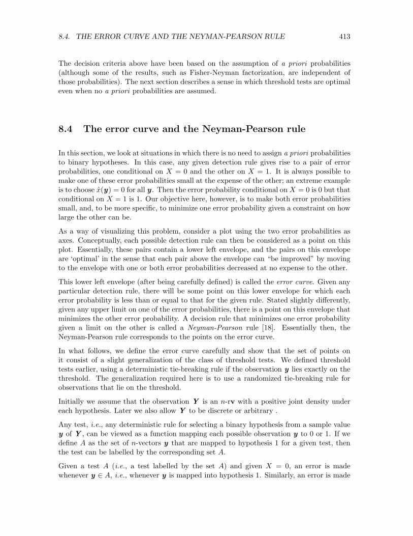
8.4 The error curve and the Neyman-Pearson rule

In this section, we look at situations in which there is no need to assign a priori probabilitiesto binary hypotheses. In this case, any given detection rule gives rise to a pair of errorprobabilities, one conditional on X = 0 and the other on X = 1. It is always possible tomake one of these error probabilities small at the expense of the other; an extreme exampleis to choose x̂(y) = 0 for all y . Then the error probability conditional on X = 0 is 0 but thatconditional on X = 1 is 1. Our objective here, however, is to make both error probabilitiessmall, and, to be more specific, to minimize one error probability given a constraint on howlarge the other can be.

As a way of visualizing this problem, consider a plot using the two error probabilities asaxes. Conceptually, each possible detection rule can then be considered as a point on thisplot. Essentially, these pairs contain a lower left envelope, and the pairs on this envelopeare ‘optimal’ in the sense that each pair above the envelope can “be improved” by movingto the envelope with one or both error probabilities decreased at no expense to the other.

This lower left envelope (after being carefully defined) is called the error curve. Given anyparticular detection rule, there will be some point on this lower envelope for which eacherror probability is less than or equal to that for the given rule. Stated slightly di↵erently,given any upper limit on one of the error probabilities, there is a point on this envelope thatminimizes the other error probability. A decision rule that minimizes one error probabilitygiven a limit on the other is called a Neyman-Pearson rule [18]. Essentially then, theNeyman-Pearson rule corresponds to the points on the error curve.

In what follows, we define the error curve carefully and show that the set of points onit consist of a slight generalization of the class of threshold tests. We defined thresholdtests earlier, using a deterministic tie-breaking rule if the observation y lies exactly on thethreshold. The generalization required here is to use a randomized tie-breaking rule forobservations that lie on the threshold.

Initially we assume that the observation Y is an n-rv with a positive joint density undereach hypothesis. Later we also allow Y to be discrete or arbitrary .

Any test, i.e., any deterministic rule for selecting a binary hypothesis from a sample valuey of Y , can be viewed as a function mapping each possible observation y to 0 or 1. If wedefine A as the set of n-vectors y that are mapped to hypothesis 1 for a given test, thenthe test can be labelled by the corresponding set A.

Given a test A (i.e., a test labelled by the set A) and given X = 0, an error is madewhenever y 2 A, i.e., whenever y is mapped into hypothesis 1. Similarly, an error is made


if X = 1 and y 2 Ac. Thus the error probabilities, given X = 0 and X = 1 respectively are

Pr{Y 2 A | X = 0} ; Pr{Y 2 Ac | X = 1} .

Note that these conditional error probabilities depend only on the test A and not on the(here undefined) a priori probabilities. We will abbreviate these error probabilities as

q0(A) = Pr{Y 2 A | X = 0} ; q1(A) = Pr{Y 2 Ac | X = 1} .

If A is a threshold test, with threshold ⌘, the set A is given by

A =⇢y :

fY |X(y | 1)fY |X(y | 0)

� ⌘

�.

Since threshold tests play a very special role here, we abuse the notation by using ⌘ in placeof A to refer to a threshold test at ⌘. That is, q0(⌘) is shorthand for Pr{e⌘ | X = 0} andq1(⌘) for Pr{e⌘ | X = 1}. We can now characterize the relationship between threshold testsand other tests. The following lemma is illustrated in Figure 8.5.

Lemma 8.4.1. Consider a two dimensional plot in which the pair�q0(A), q1(A)

�is plotted

for each A. Then for each theshold test ⌘, 0 ⌘ < 1, and each each arbitrary test A, thepoint

�q0(A), q1(A)

�lies in the closed half plane above and to the right of a straight line of

slope �⌘ passing through the point�q0(⌘), q1(⌘)

�.

bb

bb

bb

bb

bb

bb

q1(⌘) + ⌘q0(⌘)

q1(⌘)

1

1q0(⌘)✓

slope �⌘s

s�q0(A), q1(A)�b

bb

bbq1(A) + ⌘q0(A)

h⌘(✓) = q1(⌘) + ⌘�q0(⌘)� ✓

�

hA(✓) = q1(A) + ⌘�q0(A)� ✓

�

Figure 8.5: Illustration of Lemma 8.4.1

Proof: In proving the lemma, we will use Theorem 8.1.1, demonstrating9 the optimality of athreshold test for the MAP problem. As the proof here shows, that optimality for the MAPproblem (which assumes a priori probabilities) implies some properties relating q`(A) andq`(⌘) for ` = 0, 1. These quantities are defined independently of the a priori probabilities,so the properties relating them are valid in the absence of a priori probabilities.

For any given ⌘, consider the a priori probabilities (p0, p1) for which ⌘ = p0/p1. The overallerror probability for test A using these a priori probabilities is then

Pr{e(A)} = p0q0(A) + p1q1(A) = p1⇥q1(A) + ⌘q0(A)

⇤.

9Recall that Exercise 8.12 generalizes Theorem 8.1.1 to essentially arbitrary likelihood distributions.


Similarly, the overall error probability for the threshold test ⌘ using the same a prioriprobabilities is

Pr{e(⌘)} = p0q0(⌘) + p1q1(⌘) = p1⇥q1(⌘) + ⌘q0(⌘)

⇤.

This latter error probability is the MAP error probability for the given p0, p1, and is thusthe minimum overall error probability (for the given p0, p1) over all tests. Thus

q1(⌘) + ⌘q0(⌘) q1(A) + ⌘q0(A).

As shown in the figure, q1(⌘) + ⌘q0(⌘) is the point at which the straight line h⌘(✓) =q1(⌘) + ⌘

�q0(⌘)� ✓

�of slope �⌘ through

�q0(⌘), q1(⌘)

�crosses the ordinate axis. Similarly,

q1(A)+⌘q0(A) is the point at which the straight line hA(✓) = q1(A)+⌘�q0(A)� ✓

�through�

q0(A), q1(A)�

of slope �⌘ crosses the ordinate axis.. Thus all points on the second line,including

�q0(A), q1(A)

�lie in the closed half plane above and to the right of all points on

the first, completing the proof.

The straight line of slope �⌘ through the point�q0(⌘), q1(⌘)

�has the equation h⌘(✓) =

q1(⌘)+ ⌘(q0(⌘)� ✓). Since the lemma is valid for all ⌘, 0 ⌘ <1, the point�q0(A), q1(A)

�for an arbitrary test A lies above and to the right of the straight line h⌘(✓) for each ⌘, 0 ⌘ < 1. The upper envelope of this family of straight lines is called the error curve, u(✓),defined by

u(✓) = sup0⌘<1

h⌘(✓) = sup0⌘<1

q1(⌘) + ⌘(q0(⌘)� ✓). (8.66)

The lemma then asserts that for every test A (including threshold tests), we have u(q0(A)) q1(A). Also, since every threshold test lies on one of these straight lines, and therefore onor below the curve u(✓), we see that the pair

�q0(⌘), q1(⌘)

�for each ⌘ must lie on the curve

u(✓). Finally, since each of these straight lines forms a tangent of u(✓) and lies on or belowu(✓), the function u(✓) is convex.10 Figure 8.6 illustrates the error curve.

The error curve essentially gives us a tradeo↵ between the probability of error given X = 0and that given X = 1. Threshold tests, since they lie on the error curve, provide optimalpoints for this tradeo↵. Unfortunately, as we see in an example shortly, not all points on theerror curve correspond to threshold tests. We will see later, however, that by generalizingthreshold tests to randomized threshold tests, we can reach all points on the error curve.

Before proceeding to this example, note that Lemma 8.4.1 and the definition of the errorcurve apply to a broader set of models than discussed so far. First, the lemma still holds iffY |X(y | `) is zero over an arbitrary set of y for one or both hypotheses `. The likelihoodratio ⇤(y) is infinite where fY |X(y | 1) > 0 and fY |X(y | 0) = 0. This means that ⇤(Y ),conditional on X = 1, is defective, but this does not a↵ect the proof of the lemma (seeExercise 8.15 for a fuller explanation of the e↵ect of zero densities).

10A region A of a vector space is said to be convex if for every x 1, x 2 2 A, �x 1 +(1��)x 2 is also in A forall � 2 (0, 1). Examples include the entire vector space and the space of probability vectors. A function f(x )defined on a convex region A is convex if for every x 1, x 2 2 A, f(�x 1 + (1� �)x 2) �f(x 1) + (1� �)f(x 2)for all � 2 (0, 1). Examples for one dimensional regions are functions with nonnegative second derivatives,and more generally, functions lying on or above all their tangents. The latter allows for step discontinuitiesin the first derivative, which we soon see is required here.


bb

bb

bb

bb

bb

bb

q1(⌘) + ⌘q0(⌘)

q1(⌘)

1

1q0(⌘)

slope �⌘

QQk increasing ⌘

t�q0(A), q1(A)�u(✓)

✓

Figure 8.6: Illustration of the error curve u(✓) (see (8.66)). Note that u(✓) is convex,lies on or above its tangents, and on or below all tests. It can also be seen, eitherdirectly from the curve above or from the definition of a threshold test, that q1(⌘) isnon-decreasing in ⌘ and q0(⌘) is non-increasing.

In addition, it can be seen that the lemma also holds if Y is an n-tuple of discrete rv’s or ifY is a mixture of discrete and continuous components (such as being the sum of a discreteand continuous rv. With some thought, it can be seen11 that what is needed is for ⇤(Y )to be a rv conditional on X = 0 and a possibly-defective rv conditional on X = 1. We nowsummarize the results so far in a theorem.

Theorem 8.4.1. Consider a binary hypothesis testing problem in which the likelihood ratio⇤(Y) is a rv conditional on X = 0 and a possibly-defective rv conditional on X = 1. Thenthe error curve is convex, all threshold tests lie on the error curve, and all other tests lieon or above the error curve.

The following example now shows that not all points on the error curve need correspond tothreshold tests.

Example 8.4.1. A particularly simple example of a detection problem uses a discreteobservation that has only two sample values, 0 and 1. Assume that

pY |X(0 | 0) = pY |X(1 | 1) =23; pY |X(0 | 1) = pY |X(1 | 0) =

13.

In the communication context, this corresponds to a single use of a binary symmetricchannel with crossover probability 1/3. The threshold test in (8.11), using PMF’s in placeof densities, is then

⇤(y) =pY |X(y | 1)pY |X(y | 0)

x̂(y)=1�<

x̂(y)=0

⌘. (8.67)

11What is needed here is to show that threshold rules still achieve maximum a posteriori probablity ofcorrect detection in this general case. This requires a limiting argument on a quantized version of thelikelihood ratio, and is interesting primarily as an analysis exercise. An outline of such an argument is givenin Exercise 8.12.


The only possible values for y are 1 and 0, and we see that ⇤(1) = 2 and ⇤(0) = 1/2.Under ML, i.e., with ⌘ = 1, we would choose x̂(y) = y. For a threshold test with ⌘ 1/2,however, (8.67) says x̂(y) = 1 for both y = 1 and y = 0, i.e., the decision is independent ofthe observation. We can understand this intuitively in the MAP case since ⌘ 1/2 meansthat the a priori probability p0 1/3 is so small that the observation can’t overcome thisinitial bias. In the same way, for ⌘ > 2, x̂(y) = 0 for both y = 1 and y = 0. Summarizing,

x̂(y) =

8<:

1 for ⌘ 1/2y for 1/2 < ⌘ 20 for 2 < ⌘

. (8.68)

For ⌘ 1/2, we have x̂(y) = 1, so, for both y = 0 and y = 1, an error is made for X = 0but not X = 1. Thus q0(⌘) = 1 and q1(⌘) = 0 for ⌘ 1/2. In the same way, the errorprobabilities for all ⌘ are given by

q0(⌘) =

8<:

1 for ⌘ 1/21/3 for 1/2 < ⌘ 20 for 2 < ⌘

q1(⌘) =

8<:

0 for ⌘ 1/21/3 for 1/2 < ⌘ 21 for 2 < ⌘

. (8.69)

We see that q0(⌘) and q1(⌘) are discontinuous functions of ⌘, the first jumping down at⌘ = 1/2 and ⌘ = 2, and the second jumping up. The error curve for this example isgenerated as the upper envelope of the family of straight lines, {h⌘(✓); 0 ⌘ < 1} whereh⌘(✓) has slope �⌘ and passes through the point (q0(⌘), q1(⌘)). The equation for these lines,using (8.69), is as follows:

q1(⌘) + ⌘(q0(⌘)� ✓) =

8><>:

0 + ⌘(1� ✓) for ⌘ 1/213 + ⌘(1

3 � ✓) for 1/2 < ⌘ 21 + ⌘(0� ✓) for 2 < ⌘

.

The straight lines for ⌘ 1/2 pass through the point (1, 0) and sup⌘1/2[q0(⌘) + ⌘q1(⌘)]for each ✓ 1 is achieved at ⌘ = 1/2. This is illustrated in Figure 8.7. Similarly, thestraight lines for 1/2 < ⌘ 2 all pass through the point (1/3, 1/3). For each ✓ < 1/3,u(✓) = sup⌘

⇥q1(⌘)+⌘(q0(⌘)�✓)

⇤is on the line of slope -2 through the point (1/3, 1/3). The

three possible values for (q0(⌘), q1(⌘)) are shown by dots and the supremum of the tangentsis shown by the piecewise linear curve.

Let us look more carefully at the tangent of slope -1/2 through the points (1, 0) and (1/3,1/3). This corresponds to the MAP test at ⌘ = 1/2, i.e., p0 = 1/3. As seen in (8.68), thisMAP test selects x̂(y) = 1 for each y. This selection for y = 0 is a don’t-care choice forthe MAP test with ⌘ = 1/2 since ⇤(Y =0) = 1/2. If the test selected x̂(1) = 0 for ⌘ = 1/2instead, the MAP error probability would not change, but the error probability given X = 0would decrease to 1/3 and that for X = 1 would increase to 1/3.

It is not hard to verify (since there are only 4 tests, i.e., deterministic rules, for mapping abinary variable to another binary variable) that no test A can lie on an interior point of thestraight line between (1/3, 1/3) and (1, 0). However, if we use a randomized rule, mappingy = 0 to x̂ = 0 with probability � and to x̂ = 1 with probability 1� � (along with alwaysmapping 1 to 1), then all points on the straight line from (1/3, 1/3) to (1, 0) are achieved


⌘ = 1

⌘ = 4

⌘ = 1/4

q1(2)

q1(1/2)

(0, 1)s

ss(1, 0)

(1/3, 1/3)

✓ q0(2) q0(1/2)

⌘ = 1/2

⌘ = 2

u(✓)

Figure 8.7: Illustration of the error curve u(✓) for Example 8.4.1. The three pos-sible error pairs for threshold tests,

�q0(⌘), q1(⌘)

�are the indicated dots. That is

(q0(⌘), q1(⌘)) = (1, 0) for ⌘ 1/2. This changes to (1/3, 1/3) for 1/2 < ⌘ 2 andto (0, 1) for ⌘ > 2. The error curve (see (8.66)) for points to the right of (1/3, 1/3) ismaximized by the straight line of slope -1/2 through (1, 0). Similarly, the error curvefor points to the left of (1/3, 1/3) is maximized by the straight line of slope -2 (⌘ = 2)through (1/3, 1/3). One can visualize the tangent lines as an inverted see-saw, firstsee-sawing around (0,1), then around (1/3, 1/3), and finally around (1, 0).

as � goes from 0 to 1. In other words, a don’t-care choice for MAP becomes an importantchoice in the tradeo↵ between q0 and q1.

In the same way, all points on the straight line from (0, 1) to (1/3, 1/3) can be achievedby a randomized rule that maps y = 1 to x̂ = 0 with probability � and to x̂ = 1 withprobability 1� � (along with always mapping 0 to 0).

In the general case, the error curve will contain straight line segments whenever the CDFF⇤(Y )|X(⌘|0) contains discontinuities. Such discontinuities always occur for discrete obser-vations and sometimes for continuous observations (see Exercise 8.15). To see the need forthese straight line segments, assume that F⇤(Y )|X(⌘|0) has a discontinuity of size � > 0 ata given point ⌘ 2 (0,1). Then Pr{⇤(Y ) = ⌘ | X=0} = � and the MAP test at ⌘ has adon’t-care region of probability � given X = 0. This means that if the MAP test is changedto resolve the don’t-care case in favor of X = 0, then the error probability q0 is decreasedby � and the error probability q1 is increased by �⌘.

Expressing this in terms of equations, the error probabilities, given X = 0 and X = 1, witha threshold test at ⌘ have been denoted as

q0(⌘) = Pr{⇤(Y ) � ⌘ | X = 0} q1(⌘) = Pr{⇤(Y ) < ⌘ | X = 1} .

Modifying the threshold test to choose x̂ = 0 in the don’t care cases for MAP, the resultingerror probabilities are denoted as eq0(⌘) and eq1(⌘), where

eq0(⌘) = Pr{⇤(Y ) > ⌘ | X = 0} eq1(⌘) = Pr{⇤(Y ) ⌘ | X = 1} . (8.70)

What we just showed is that if Pr{⇤(Y ) = ⌘ | X = 0} = �, then

eq0(⌘) = q0(⌘)� �; eq1(⌘) = q1(⌘) + ⌘�.


Lemma 8.4.1 is easily seen to be valid whichever way the MAP don’t-care cases are resolved,and thus both (q0(⌘), q1(⌘)) and (eq0(⌘), eq1(⌘)) lie on the error curve. Since all tests lie aboveand to the right of the straight line of slope �⌘ through these points, the error curve hasa straight-line segment between these points. As explained in the example, points on thestraight line between (eq0(⌘), eq1(⌘)) and (q0(⌘), q1(⌘)) can be realized by resolving thesedon’t care cases in a random fashion.

Definition 8.4.1. A randomized threshold rule at ⌘ is a rule that detects x̂ = 0 for ⇤(y) <⌘, x̂ = 1 for ⇤(y) > ⌘ and detects x̂ = 0 with some given probability �, 0 < � < 1 and x̂ = 1with probability 1� � for ⇤(y) = ⌘.

As in the example, if there is a straight line segment of slope �⌘ on the error curve, then arandomized threshold rule at ⌘ achieves each point on the straight line from (eq0(⌘), eq1(⌘))to (q0(⌘), q1(⌘)) as � goes from 0 to 1.

8.4.1 The Neyman-Pearson detection rule

Definition 8.4.2. A Neyman Pearson rule is a binary detection rule (perhaps randomized)that, given the constraint that Pr{e | X=0} ✓, satisfies Pr{e | X=1} u(✓) where u(✓)is given in (8.66).

Given the error curve, u(✓), we have essentially seen how to construct a Neyman-Pearsonrule. The point (✓, u(✓)) either corresponds to a threshold test at one or more values of ⌘,or it lies on a straight line of slope ⌘ between two threshold tests. In the first case, thethreshold test at ⌘ is a Neyman-Pearson rule, and in the second case a randomized thresholdrule, choosing x̂ = 1 for ⇤(y) > ⌘, choosing x̂ = 0 for ⇤(y) < ⌘ and choosing randomlywhen ⇤(y) = ⌘.

This is summarized in the following theorem; the proof clarifies a couple of points thatmight have been confusing above.

Theorem 8.4.2. Consider a binary hypothesis testing problem in which the likelihood ratio⇤(Y) is a rv conditional on X = 0 and a possibly-defective rv conditional on X = 1. Thenfor any detection rule and any ✓, 0 < ✓ < 1, the constraint that Pr{e | X = 0} ✓ impliesthat Pr{e | X = 1} � u(✓) where u(✓) is the error curve. Furthermore, Pr{e | X = 1} =u(✓) if the Neyman-Pearson rule for ✓ is used.

Proof: For any given ⌘, the threshold test at ⌘ makes at error given X = 0 if ⇤ � ⌘. Thethreshold rule modified to map don’t-care cases to 0 makes an error if ⇤ > ⌘, i.e.,

eq0(⌘) = 1� F⇤|X(⌘|0); q0(⌘) = 1� F⇤|X(⌘|0)� Pr{⇤=⌘ | X=0}

Since F⇤|X(⌘|0) is a distribution function, it can have discontinuities, but if it has a discon-tinuity at ⌘ the discontinuity has size Pr{⇤=⌘ | X=0} and must lie between 1� q0(⌘) and1 � eq0(⌘). This means that for any ✓ 2 (0, 1), there is either an ⌘ for which ✓ = q0(⌘) orthere is an ⌘ for which eq0(⌘) ✓ < q0(⌘). Thus either a threshold test at ⌘ can be used ora randomized threshold test at ⌘ can be used for a Neyman-Pearson rule.


Theorem 8.4.1 shows that any deterministic test has error probabilities lying on or abovethe error curve. The question remaining is whether an arbitrary randomized rule can liebelow the error curve. A randomized rule is a convex combination of a set of deterministicrules (i.e., it uses each of the deterministic tests with a probability that adds to 1 over theset of tests). However, a convex combination of points each above the error curve must alsobe above the error curve.

8.4.2 The min-max detection rule

A final interesting example of a randomized threshold rule is the min-max rule. This is arule that minimizes the maximum of the two error probabilities, q0(A) and q1(A). Now ifthe pair (q0(A), q1(A)) does not lie on the error curve, then the maximum of the two (orboth together if they are equal) can be reduced. We have seen that all points on the errorcurve correspond either to threshold tests or to randomized threshold rules, so for any pair(q0(A), q1(A)), there is either a threshold test or randomized threshold rule that is at leastas good in the min-max sense.

We can see geometrically that the error probabilities for a min-max rule must lie at theintersection of the error curve with the 45o line through the origin. Since this point is onthe error curve, it can be achieved either by a threshold rule or a randomized thresholdrule.

8.5 Finitely many hypotheses

Consider hypothesis testing problems with M � 2 hypotheses. In a Bayesian setting, X isthen a random variable with the possible values 0, 1, . . . ,M � 1 and a priori probabilitiesp0, . . . , pM�1. Assume that for each `, there is a cost C` of making an incorrect decision,i.e., the cost is C` if X = ` and x̂ 6= ` . We assume that this cost depends neither on theobservation y nor the particular incorrect decision. A minimum cost test is a decision rulethat minimizes the expected cost of a decision.

In this section, we analyze minimum-cost tests for M � 2 and compare them with M = 2as analyzed in Section 8.3. If C` = 1 for all `, then a minimum-cost test is a MAP test,so MAP is a special case of min-cost. For an observed sample value y of the observationrvY , we can compare the expected costs of di↵erent decisions,

E [cost of x̂=k | Y=y ] =X6̀=k

C` pX|Y (` | y) (8.71)

=X

`

C` pX|Y (j | y)� Ck pX|Y (k | y). (8.72)

Since the sum on the right hand side of (8.72) is common to all k, the expected cost ofmaking decision k is minimized by choosing the hypothesis for which an error would be

8.5. FINITELY MANY HYPOTHESES 421

most costly, i.e.,

x̂(y) = arg maxk

Ck pX|Y (k | y). (8.73)

This conforms with intuition, which would weight both the a posteriori probability ofthe hypothesis and the cost of an error. It improves intuition by specifing the weighting.Assuming that the observation y has a positive probability density conditional on eachhypothesis, we have

pX|Y (k | y) =

pkfY |k(y)fY (y)

; x̂(y) = arg maxk

Ck pkfY |X(y | k)). (8.74)

Defining the likelihood ratio ⇤`k(y) = fY |X(y | l)/fY |X(y | k), the maximization in (8.74)can be viewed as a set of binary threshold comparisons, i.e., for all `, k with ` > k

⇤`k(y) =fY |X(y | l)fY |X(y | k)

x̂(y)6=k�<

x̂(y)6=`

Ckpk

C`p`= ⌘`k. (8.75)

The meaning of (8.75) is that a threshold test between ` and k rejects either ` or k (whileusing the same arbitrary tie-breaking rule as in the binary case). After eliminating either` or k as the min-cost decision, the remaining contender must still be tested against theother possibilities. If these binary choices are made sequentially, each time comparing 2 yetunrejected hypotheses, then each binary test eliminates one contender and M � 1 binarytests are needed to establish the minimum-cost choice among the M hypotheses.

This procedure is essentially the same as an athletic tournament in which each binary gameeliminates one team, with the ultimate survivor winning the tournament.

The meaning of the above tournament when some of the likelihoods are zero requires someinterpretation. We assume as usual that the region for which all the likelihoods are 0 isignored. Then if a likelihood ratio is 0 or1, the 0 likelihood hypothesis is eliminated. If thelikelihood ratio is undefined (both likelihoods are zero), then it makes no di↵erence whichhypothesis is eliminated, since the other will eventually be eliminated by an hypothesis withpositive likelihood. In essence, the tournament above, combined with common sense, findsa min-cost hypothesis.

Example 8.5.1. Consider the same communication situation as in Figure 8.4, but assumethe source alphabet is {0, 1, . . . ,M�1}. The letter to be transmitted, say `, is mapped into asignal a` = (a`1, a`2, . . . , a`n). The noise in each dimension is IID Gaussian, N (0,�2). Thelog-likelihood ratio evaluated in (8.41), applied to any given pair, say ` > k, of hypothesesis given by

LLR`k(y) =(a` � ak)T

�2

✓y � a` + ak

2

◆ x̂(y)6=k�<

x̂(y)6=`

ln(⌘`k). (8.76)

The threshold ⌘`k (as defined in (8.75)) is 1 for the maximum likelihood (ML) case, pk/p`

for the MAP case, and pkCk/(p`C`) for the min-cost case.


The geometric interpretation of this, in the space of observed vectors y , is shown for theML case in Figure 8.8. The decision threshold between each pair of hypotheses is theperpendicular bisector of the line joining the two signals. Note that (a` � ak)Ty is asu�cient statistic for the binary test between ` and k. Thus if the dimension n of theobserved vectors y is greater than M� 1, we can reduce the problem to M� 1 dimensionsby transforming to a co-ordinate basis in which, for each j, 1 j m�1, aj�a0 is a linearcombination of M � 1 (or perhaps fewer) basis vectors. Using the theorem of irrelevance,the components of y in all other directions can be ignored.

&%'$ra0

&%'$ra2

r&%'$

a1

x̂ = 0

x̂ = 1

x̂ = 26

-

�

@@Rx̂ = 1

Figure 8.8: Decision regions for an 3-ary alphabet of vector signals in IID Gaussiannoise. For ML detection, the decision regions are Voronoi regions, i.e., regions separatedby perpendicular bisectors between the signal points. For the MAP case with unequal apriori probabilities, or the min-cost case, these perpendicular bisectors are shifted whileremaining perpendicular to the straight lines between the signal points

Even after the simplification of representing an additive Gaussian noise M-ary detectionproblem in the appropriate M� 1 or fewer dimensions, calculating the probability of errorfor each hypothesis can be messy. For example, in Figure 8.8, Pr{e | X=2} is the probabilitythat the noise, added to a2, carries the observation y outside of the region where x̂ = 2.

This can be evaluated numerically using a two dimensional integral over the given constraintregion. In typical problems of this type, however, the boundaries of the constraint regionare several standard deviations away from a2 and the union bound is often su�cient toprovide a good upper bound to the error probability. That is, the error event, conditionalon X = k, is the union of the events that the individual binary thresholds are crossed.Thus, using (8.76),

Pr{e | X=k} X6̀=k

Pr⇢

(a` � ak)T

�2

✓y � a` + ak

2� ln ⌘`k

◆�. (8.77)

Using (8.44) to evaluate the terms on the right hand side,

Pr{e | X=k} X6̀=k

Q

✓� ln(⌘`k)ka` � akk

+ka` � akk

2�

◆. (8.78)


Example 8.5.2. As a yet further simplified version of Example 8.5.1, suppose that M = 4and the 4 signal points are�3b, �b, b, 3b for some arbitrary vector b. Then a` = (2`�3)bfor each signal a`, 0 ` 3. From (8.76), the log-likelihood ratios and threshold tests are

LLR`k(y) =2(`� k)bT

�y � (` + k � 3)b

��2

x̂(y)6=k�<

x̂(y)6=`

ln(⌘`k). (8.79)

As one might expect, each LLR depends on y only through bTy , so in this case bTy is asu�cient statistic for all of the log-likelihood ratios. If the test is ML, then ln(⌘`k) = 0 forall `, k and the decision regions (in terms of bTy) are illustrated in Figure 8.9.

a1 a2 a3a0

x̂ = 1 x̂ = 2 x̂ = 3x̂ = 0

0b -

Figure 8.9: Decision regions for a 4-ary alphabet of co-linear vector signals in IIDGaussian noise. The log-likelihood ratios depend on y only through the one-dimensionalsu�cient statistic aTy . For ML detection, the decision regions are intervals over aTybounded by the points half way between the signal points.

The error probability (for ML detection) can be worked out exactly for this example byinspection. For the outer two signal points, an error can be made only by noise exceedingkbk in the direction toward the inner points. For the two inner points, an error is made ifthe noise exceeds kbk in either direction. Thus

Pr{e | X = k} =

8><>:

Q⇣kbk�

⌘for k = 0, 3

2Q⇣kbk�

⌘for k = 1, 2

.

8.5.1 Su�cient statistics with M � 2 hypotheses

We have just shown that min-cost, MAP, and ML decisions can be made between M � 2hypotheses by using a tournament between binary threshold tests. Each of these binarytests might be simplified by the use of a su�cient statistic for that binary test. In Example8.5.2, the same su�cient statistic worked for each binary test, and this section shows howto handle more general cases. What we want is a single function (often multidimensional)of the observation y that works as a su�cient statistic for all the binary tests.

Definition 8.5.1 (Su�cient statistic; M � 2). For hypothesis testing with M � 2 hy-potheses, {0, . . . ,M�1}, a su�cient statistic is any function v(y) of the observation yfrom which each binary likelihood ratio can be calculated, i.e., for which a set of functionsu`k; 0 k < ` M� 1 exists such that ⇤`k(y) = u`k(v(y)) .


As in the case of binary hypotheses, there are several equivalent conditions that could beused as a definition, and each provides its own insights. For a large number of hypothe-ses, this original definition is somewhat awkward because of the large number of binarycomparisons replacing what is essentially the choice of a maximum term. The definitioninvolves a set of M(M� 1)/2 functions, u`k(v(y), but these functions are highly redundantsince the corresponding set of likelihood ratios in the definition are composed from only Mlikelihoods. The equivalent definitions we now establish are virtually the same as in thebinary case, but do not su↵er this increase in complexity.

We state the following theorem in terms of continuous observations (thus again omittingthe first part of Theorem 8.2.3, which could be included for the discrete case).

Theorem 8.5.1. Let V = v(Y) be a function of Y for an hypothesis rv X with M samplevalues and with a continuous observation Y. The following (for all sample values y) areequivalent conditions for v(y) to be a su�cient statistic:

1. A set of functions u`k(v) exists such that ⇤`k(y) = u`k�v(y)

�for each 0 ` < k

M� 1.


pX|Y(k | y) = p

X|V

�k | v(y)

�for 0 k M� 1. (8.80)

3. The likelihood ratio of y is the same as that of v(y), i.e., if V has a density,

⇤`k(y) =fV|X

�v(y) | `

�fV|X

�v(y) | k

� . (8.81)

4. Functions �(y) and eux�v(y)

�exist for 0 x M� 1 such that

fY|X (y | x) = �(y) eux

�v(y)

�. (8.82)

Proof: The proof is very similar to those for Theorems 8.2.2 and 8.2.3, so identical detailsare omitted. We show that condition 1 implies 2 implies 3 implies 1, and then that 2 implies4 implies 1. Starting with Bayes’ law followed by the use of condition 1,

pX|Y (k | y) =

pk fY |X (y | k))PM�1

`=0 p`fY |X (y | `))

=pkPM�1

`=0 p`⇤`k(y)=

pkPM�1`=0 p`u`k

�v(y)

� ,

where uk,k(v) is taken to be 1 and u`k�v(y)

�=⇥uk,`

�v(y)

�⇤�1 for ` > k. This shows thatp

X|Y (0 | y) is a function of y only through v(y), i.e., that pX|Y (0 | y) is the same for all

y with a common value of v(y). Thus pX|Y (` | y) is the conditional probability of X = `

given V = v(y). This establishes (8.80).


Next we show that condition 2 implies condition 3. Taking the ratio of (8.80) for X = ` tothat for X = k,

pX|Y (` | y)

pX|Y (k | y)

=p

X|V

�` | v(y)

�p

X|V

�k | v(y)

� .

Applying Bayes’ law to each numerator and denominator above and cancelling fY (y) fromboth terms on the left, fV

�v(y)

�from both terms on the right, and p` and pk throughout,

we get (8.81). The argument is essentially the same if V has a PMF or a mixed distribution.

Going from condition 3 to 1 is obvious, since the right side of (8.81) is a function of y onlythrough v(y).

To prove condition 4 from 2, assume that v(y) satisfies (8.80) for given {p0, . . . , pM�1}.Choose �(y) = fY (y). Then to satisfy (8.82), we must have

eu`�v(y)

�=

fY |X (y | `)

fY (y)=

pX|Y (` | y)

p`=

pX|V

�` | v(y)

�p`

.

This indeed depends on y only through v(y).

Finally, assume v(y) satisfies (8.82). Taking the ratio of (8.82) for x = ` to that for x = k,the term �(y) cancels. Thus condition 1 is satisfied by choosing u`k = eu`/euk.

Example 8.5.3. Consider the 4 co-linear signals in Gaussian noise of Example 8.5.2 again.Assuming that the observation is n-dimensional, we have

fY |X (y | `) = (2⇡�2)n/2 exp

nXj=1

�(yj � (2`� 3)bj)2

2�2

=

"(2⇡�2)n/2 exp

Xn

j=1

�y2j

2�2

# exp

2(2`� 3)bTy � (2`� 3)2bTb

2�2

�.

The first factor above is a function of y and does not depend on ` (it is simply the densityof the n-dimensional noise) and the second term is a function of both ` and bTy . Thusthese terms can be chosen as �(y) and eu`(v(y)) in (8.82). Note that this choice is just asnatural as the choice of fY (y) for �(y) used in the proof of Theorem 8.5.1.

8.5.2 More general min-cost tests

Section 8.3 discussed min-cost decisions for binary hypotheses. In one formulation (the onefollowed earlier in this section), C` is taken to be the cost of an error when X = `. In theother, more general, formulation, C`,k is taken to be the cost for X = ` and x̂ = k. In thissection we consider that more general formulation for M � 2 hypotheses. In the binarycase, the more general formulation simply complicated the notation. Here it has a morefundamental e↵ect.


For this more general set of costs, the expected cost of deciding on a given hypothesis,k, 0 k M�1 is given by

E [cost of x̂=k | Y=y ] =M�1X`=0

C`,k pX|Y (` | y).

The min-cost decision minimizes this sum for each observation y , i.e.,

x̂(y) = arg mink

M�1X`=0

C`,k pX|Y (` | y). (8.83)

We use the usual convention of choosing the largest numbered decision in the case of a tie.

This decision can not be put in the form of a tournament of binary threshold decisions,although it could be viewed as a tournament of more complicated binary decisions, wherethe binary decision between k and j, say, would involve C`,k and C`,j for all `.

This decision can be made in terms of a su�cient statistic, v(y) for the observation y . Tosee this, we simply replace p

X|Y (` | y) in 8.83 by pX|V

�` | v(y)

�.

This substitution is justified by condition 2 of Theorem 8.5.1. There does not seem to bemuch more of general interest that can be said of these more general min-cost decisions.

8.6 Summary

The mathematical problem studied in this chapter is very simple. A probability spacecontains a discrete rv X with a finite set of sample values (hypotheses) and contains arandom vector Y whose sample values are called observations. We are to choose a functionx̂(y) that maps each observation y into an hypothesis. This function is called a decision,a detected value, or a choice of hypothesis, and there are a number of possible criteria forchoosing this function.

The simplest criterion is the maximum a posteriori probability (MAP) criterion, wherefor each y , x̂(y) maximizes Pr{X = x̂(y) | Y = y}. In the case of a tie, the largest suchx̂(y) is arbitrarily chosen. This criterion (almost obviously) also maximizes the overallprobability of correct choice, averaged over Y .

A slightly more general criterion is the min-cost criterion, where for each hypothesis k, thereis a cost Ck of choosing incorrectly (choosing x̂(y) 6= k) when X = k. The min-cost decisionchooses x̂(y) to minimize expected cost (with the same tie-breaking rule as before). MAPis thus a special case of min-cost for which Ck = 1 for each k.

If X is binary, then min-cost and MAP detection are threshold tests where the likelihoodratio ⇤(y) = f

Y |X (y | 1)/fY |X (y | 0) is compared with a numerical threshold ⌘. For min-cost,

⌘ = C0p0/C1p1 where (p0, p1) are the a priori probabilities of X.

Both threshold tests and the corresponding expected costs or error probabilities can oftenbe simplified by a function v(y) called a su�cient statistic and defined by the property that

8.6. SUMMARY 427

⇤(y) is a function of v(y). There are a number of equivalent definitions of su�cient statisticsfor binary hypotheses specified by Theorems 8.2.2, 8.2.3, and 8.2.4. Several examples,including detection of a binary signal in various forms of Gaussian noise and detection ofthe rate of a Poisson process, illustrate the usefulness of su�cient statistics.

There are a number of both practical and theoretical reasons for having decision criteriathat do not depend on a priori probabilities. One such criterion is the maximum-likelihood(ML) criterion, which is the same as the MAP criterion with p0 = p1. A more fundamentalcriterion is the Neyman-Pearson criterion, which minimizes Pr{e | X = 1} subject to a givenupper bound on Pr{e | X = 0}. As the bound on Pr{e | X = 0} is varied from 0 to 1, theminimum value of Pr{e | X = 1} traces out a curve called the error curve. The points onthe error curve are the threshold tests as ⌘ varies from 0 to 1, combined with randomizedrules to break ties in the threshold rule, thus providing flexibility in proportioning betweenerror types.

For hypothesis testing with M � 2 hypotheses, MAP tests and min-cost tests can be real-ized by a tournament of threshold tests. This provides a straightforward generalization ofthe results for binary hypothesis testing, and is often useful in understanding the regionsof observations that are mapped into each of the hypotheses. It is often more straightfor-ward to view MAP and min-cost tests simply as optimizations over the set of hypotheses.The equivalent definitions of su�cient statistics generalize for M � 2, and some of thosedefinitions are useful in viewing the tests as straightforward optimizations. The Neyman-Pearson test can also be generalized for M � 2. It then minimizes the error probability ofone hypothesis given upper bounds on all the others.


8.7 Exercises

Exercise 8.1. In this exercise, we evaluate Pr{e⌘ | X = a} and Pr{e⌘ | X = b} for binarydetection from vector signals in Gaussian noise directly from (8.40) and(8.41).

a) By using (8.40) for each sample value y of Y , show that

E [LLR(Y ) | X=a ] =�(b � a)T(b � a)

2�2.

Hint: Note that, given X = a , Y = a + Z .

b) Defining � = kb � ak/(2�), show that

E [LLR(Y ) | X=a ] = �2�2.

c) Show that

VAR [LLR(Y ) |X=a ] = 4�2.

Hint: Note that the fluctuation of LLR(Y ) conditional on X = a is (1/�2)(b � a)TZ .

d) Show that, conditional on X = a , LLR(Y ) ⇠ N (�2�2, 4�2). Show that, conditional onX = a , LLR(Y /2�) ⇠ N (��, 1).

e) Show that the first half of (8.44) is valid, i.e., that

Pr{e⌘ | X=a} = Pr{LLR(Y )� ln ⌘ |X=a} = Q

✓ln ⌘

2�+ �

◆.

f) By essentially repeating parts a) through e), show that the second half of (8.44) is valid,i.e., that

Pr{e⌘ | X =b} = Q

✓� ln ⌘

2�+ �

◆.

Exercise 8.2. (Generalization of Exercise 8.1) a) Let U = (b � a)TK�1Z Y . Find E [U | X=a ]

and E [U | X=b].

b) Find the conditional variance of U conditional on X = a . Hint: see the hint in part cof Exercise 8.1

c) Give the threshold test in terms of the sample value u of U, and evaluate Pr{e⌘ | X=a}and Pr{e⌘ | X=b} from this and part b). Show that your answer agrees with (8.53) .

d) Explain what happens if [KZ ] is singular. Hint: you must look at two separate cases,depending on the vector b � a .

Exercise 8.3. a) Let Y be the observation rv for a binary detection problem, let y be theobserved sample value. Let v = v(y) be a su�cient statistic and let V be the correspondingrandom variable. Show that ⇤(y) is equal to p

V |X (v(y) | b)/pV |X (v(y) | a). In other words,

8.7. EXERCISES 429

show that the likelihood ratio of a su�cient statistic is the same as the likelihood ratio ofthe original observation.

b) Show that this also holds for the ratio of probability densities if V is a continuous rv orrandom vector.

Exercise 8.4. a) Show that if v(y) is a su�cient statistic according to condition 1 ofTheorem 8.2.2, then

pX|Y V

�x | y , v(y)

�= p

X|Y (x | y).

b) Consider the subspace of events conditional on V (y) = v for a given v. Show that for ysuch that v(y) = v,

pX|Y V

�x | y , v(y)

�= p

X|V (x | v).

c) Explain why this argument is valid whether Y is a discrete or continuous random vectorand whether V is discrete, continuous or part discrete and part continuous.

Exercise 8.5. a) Let Y be a discrete observation random vector and let v(y) be a functionof the sample values of Y . Show that

pY |V X

�y | v(y), x

�=

pY |X (y | x)

pV |X

�v(y) | x)

.

b) Using Theorem 8.2.2, show that the above fraction is independent of X if and only ifv(y) is a su�cient statistic.

c) Now assume that Y is a continuous observation random vector, that v(y) is a givenfunction, and V = v(Y ) has a probability density. Define

fY |V X

(y | v(y), x) =fY |X (y | x)

fV |X

�v(y) | x

� .

One can interpret this as a strange kind of probability density on a conditional samplespace, but it is more straightforward to regard it simply as a fraction. Show that v(y)is a su�cient statistic if and only if this fraction is independent of x. Hint: Model yourderivation on that in part b), modifying part b) as necessary to do this.

Exercise 8.6. Consider Example 8.2.4, and let Z = [A]W where W ⇠ N (0, I) is normal-ized IID Gaussian and [A] is non-singular. The observation rv Y is a + Z given X = aand is b + Z given X = b. Suppose the observed sample value y is transformed intov = [A�1]y . Explain why v is a su�cient statistic for this detection problem (and thuswhy MAP detection based on v must yield the same decision as that based on y).

b Consider the detection problem where V = [A�1]a + W given X = a and [A�1]b + Wgiven X = b. Find the log-likelihood ratio LLR(v) for a sample value v of V . Show thatthis is the same as the log-likelihood ratio for a sample value y = [A]v of Y .


c) Find Pr{e | X=a} and Pr{e | X=b} for the detection problem in part b) by using theresults of Example 8.2.3. Show that your answer agrees with (8.53). Note: the methodologyhere is to transform the observed sample value to make the noise IID; this approach is oftenboth useful and insightful.

Exercise 8.7. Binary frequency shift keying (FSK) with incoherent reception can be mod-eled in terms of a 4 dimensional observation vector Y = (Y1, Y2, Y3, Y4)T. Y = U + Zwhere Z ⇠ N (0,�2I) and Z is independent of X. Under X = 0, U = (a cos�, a sin�, 0, 0)T,whereas under X = 1, U = (0, 0, a cos�, a sin�)T. The random variable � is uniformly dis-tributed between 0 and 2⇡ and is independent of X and Z . The a priori probabilities arep0 = p1 = 1/2.

a) Convince yourself from the circular symmetry of the situation that the ML receivercalculates the sample values v) and v1 of V0 = Y 2

1 + Y 22 and V1 = Y 2

3 + Y 24 and chooses

x̂ = 0 if v0 � v1 and chooses x̂ = 1 otherwise.

b) Find Pr{V1 > v1 | X=0} as a function of v1 > 0.

c) Show that

pY1,Y2|X,�

(y1, y2 | 0, 0) =1

2⇡�2exp

�y2

1 � y22 + 2y1a� a2

2�2

�.

d) Show that

Pr{V1 > V0 | X=0,�=0} =Z

pY1,Y2|X,�(y1, y2 | 0, 0)Pr�V1 > y2

1 + y22

dy1dy2.

Show that this is equal to (1/2) exp(�a2/(4�2).

e) Explain why this is the probability of error (i. e., why the event V1 > V0 is independentof �), and why Pr{e | X=0} = Pr{e | X=1}.

Exercise 8.8. Binary frequency shift keying (FSK) on a Rayleigh fading channel can bemodeled in terms of a 4 dimensional observation vector Y = (Y1, Y2, Y3, Y4)T. Y = U + Zwhere Z ⇠ N (0,�2I) and Z is independent of U . Under X = 0, X = (U1, U2, 0, 0)T,whereas under X = 1, U = (0, 0, U3, U4)T. The random variables Ui ⇠ N (0, a2) are IID.The a priori probabilities are p0 = p1 = 1/2.

a) Convince yourself from the circular symmetry of the situation that the ML receivercalculates sample values v0 and v1 for V0 = Y 2

1 + Y 22 and V1 = Y 2

3 + Y 24 and chooses x̂ = 0

if v0 > v1 and chooses x̂ = 1 otherwise.

b) Find fV0|X

(v0 | 0) and find fV1|X

(v1 | 0).

c) Let W = V0 � V1 and find fW (w | X=0).

d) Show that Pr{e | X=0} = [2 + a2/�2)]�1. Explain why this is also the unconditionalprobability of an incorrect decision.

8.7. EXERCISES 431

Exercise 8.9. A disease has two strains, 0 and 1, which occur with a priori probabilitiesp0 and p1 = 1� p0 respectively.

a) Initially, a rather noisy test was developed to find which strain is present for patients withthe disease. The output of the test is the sample value y1 of a random variable Y1. Givenstrain 0 (X=0), Y1 = 5 + Z1, and given strain 1 (X=1), Y1 = 1 + Z1. The measurementnoise Z1 is independent of X and is Gaussian, Z1 ⇠ N (0,�2). Give the MAP decision rule,i.e., determine the set of observations y1 for which the decision is x̂=1. Give Pr{e | X=0}and Pr{e | X=1} in terms of the function Q(x)

b) A budding medical researcher determines that the test is making too many errors. Anew measurement procedure is devised with two observation random variables Y1 and Y2.Y1 is the same as in part a). Y2, under hypothesis 0, is given by Y2 = 5 + Z1 + Z2, and,under hypothesis 1, is given by Y2 = 1 + Z1 + Z2. Assume that Z2 is independent of bothZ1 and X, and that Z2 ⇠ N (0,�2). Find the MAP decision rule for x̂ in terms of the jointobservation (y1, y2), and find Pr{e | X=0} and Pr{e | X=1}. Hint: Find f

Y2|Y1,X(y2 | y1, 0)

and fY2|Y1,X

(y2 | y1, 1).

c) Explain in laymen’s terms why the medical researcher should learn more about proba-bility.

d) Now suppose that Z2, in part b), is uniformly distributed between 0 and 1 rather thanbeing Gaussian. We are still given that Z2 is independent of both Z1 and X. Find theMAP decision rule for x̂ in terms of the joint observation (y1, y2) and find Pr(e | X=0) andPr(e | X=1).

e) Finally, suppose that Z1 is also uniformly distributed between 0 and 1. Again find theMAP decision rule and error probabilities.

Exercise 8.10. a) Consider a binary hypothesis testing problem, and denote the hypothe-ses as X =1 and X =�1. Let a = (a1, a2, . . . , an)T be an arbitrary real n-vector and let theobservation be a sample value y of the random vector Y = Xa +Z where Z ⇠ N (0,�2In)and In is the n ⇥ n identity matrix. Assume that Z and X are independent. Find themaximum likelihood decision rule and find the probabilities of error Pr(e | X = 0) andPr(e | X=1) in terms of the function Q(x).

b) Now suppose a third hypothesis, X =0, is added to the situation of part a). Again theobservation random vector is Y = Xa + Z , but here X can take on values �1, 0, or +1.Find a one dimensional su�cient statistic for this problem (i.e., a one dimensional functionof y from which the likelihood ratios

⇤1(y) =p

Y |X (y | 1)p

Y |X (y | 0)and ⇤�1(y) =

pY |X (y | �1)p

Y |X (y | 0)

can be calculated).

c) Find the maximum likelihood decision rule for the situation in part b) and find theprobabilities of error, Pr(e | X=x) for x = �1, 0,+1.


d) Now suppose that Z1, . . . , Zn in part a) are IID and each is uniformly distributed overthe interval �2 to +2. Also assume that a = (1, 1, . . . , 1)T. Find the maximum likelihooddecision rule for this situation.

Exercise 8.11. A sales executive hears that one of his salespeople is routing half of hisincoming sales to a competitor. In particular, arriving sales are known to be Poisson at rateone per hour. According to the report (which we view as hypothesis X=1), each secondarrival is routed to the competition; thus under hypothesis 1 the interarrival density forsuccessful sales is f(y|X=1) = ye�y; y � 0. The alternate hypothesis (X=0) is that therumor is false and the interarrival density for successful sales is f(y|X=0) = e�y; y � 0.Assume that, a priori, the hypotheses are equally likely. The executive, a recent student ofstochastic processes, explores various alternatives for choosing between the hypotheses; hecan only observe the times of successful sales however.

a) Starting with a successful sale at time 0, let Si be the arrival time of the ith subse-quent successful sale. The executive observes S1, S2, . . . , Sn(n � 1) and chooses the maxi-mum aposteriori probability hypothesis given this data. Find the joint probability densityf(S1, S2, . . . , Sn|X=1) and f(S1, . . . , Sn|X=0) and give the decision rule.

b) This is the same as part a) except that the system is in steady state at time 0 (ratherthan starting with a successful sale). Find the density of S1 (the time of the first arrival aftertime 0) conditional on X=0 and on X=1. What is the decision rule now after observingS1, . . . , Sn.

c) This is the same as part b), except rather than observing n successful sales, the successfulsales up to some given time t are observed. Find the probability, under each hypothesis,that the first successful sale occurs in (s1, s1 + �], the second in (s2, s2 + �], . . . , and thelast in (sN(t), sN(t) + �] (assume � very small). What is the decision rule now?

Exercise 8.12. This exercise generalizes the MAP rule to cases where neither a PMF norPDF exist. To view the problem in its simplest context, assume a binary decision, a one-dimensional observation (y 2 R1), and fixed a priori probabilities p0, p1. An arbitrary test,denoted test A, can be defined by the set A of observations that are mapped into decisionx̂ = 1. Using such a test, the overall probability of correct decision is given by (8.6) as

PrnX̂A(Y ) = X

o= p0Pr{Y 2 Ac | X = 0}+ p1Pr{Y 2 A | X = 1} . (8.84)

The maximum of this probability over all tests A is then

supA

PrnX̂A(Y ) = X

o= sup

A

⇥p0Pr{Y 2 Ac | X = 0}+ p1Pr{Y 2 A | X = 1}

⇤. (8.85)

We first consider this supremum over all A consisting of a finute union of disjoint intervals.Then (using measure theory), we show that the supremum over all measurable sets A is thesame as that over finite unions of disjoint intervals.

a) If A is a union of k intervals, show that Ac is a union of at most k + 1 disjoint intervals.Intervals can be open or closed on each end and can be bounded by ±1.

8.7. EXERCISES 433

b) Let I be the partition of R created by the intervals of both A and of Ac. Let Ij be thejth interval in this partition. Show that

Pr{x̂A(Y ) = X} X

j

maxhp0Pr{Y 2 Ij | X = 0} , p1Pr{Y 2 Ij | X = 1}

i.

Hint: Break (8.84) into intervals and apply the MAP principle on an interval basis.

c) The expression on the right in part b is a function of the partition but is otherwisendependent of A. It corresponds to a test where Y is first quantized to a finite set ofintervals, and the MAP test is then applied to this discrete problem. We denote this testas MAP(I). Let the partition I 0 be a refinement of I in the sense that each interval of I 0is contained in some interval of I. Show that

Prnx̂

MAP(I)(Y ) = X

o Pr

nx̂

MAP(I0)(Y ) = Xo

.

d) Show that for any two finite partitions of R into intervals, there is a third finite partitionthat is a refinement of each of them.

e) Consider a sequence {Aj , j � 1} (each is a finite union of intervals) that approachesthe sup (over finite unions of intervals) of (8.85). Demonstrate a corresponding sequence ofsuccessive refinements of partitions {Ij , j � 1} for which Pr

nx̂

MAP(Ij)(Y ) = X

oapproaches

the same limit.

Note what this exercise has shown so far: if the likelihoods have no PDF or PMF, thereis no basis for a MAP test on an individual observation y. However, by quantizing theobservations su�ciently finely, the quantized MAP rule has an overall probability of beingcorrect that is as close as desired to the optimum over all rules where A is a finite (butarbitrarily large) union of intervals. The arbitrarily fine quantization means that the de-cisions are arbitrarily close to pointwise decisions, and the use of quantization means thatinfinitely fine resolution is not required for the observations.

f) Next suppose the supremum in (8.85) is taken over all measureable sets A 2 R. Showthat, given any measurable set A and any ✏ > 0, there is a finite union of intervals A0 suchthat Pr{A 6= A0 | X = `} ✏ both for ` = 0 and ` = 1. Show from this that the sup in(8.85) is the same whether taken over measurable sets or finite unions of intervals.

Exercise 8.13. For the min-cost hypothesis testing problem of Section 8.3, assume thatthere is a cost C0 of choosing X=1 when X=0 is correct, and a cost C1 of choosing X=0when X=1 is correct. Show that a threshold test minimizes the expected cost using thethreshold ⌘ = (C1p1)/(C0p0).

Exercise 8.14. a) For given ✓, 0 < ✓ 1, let ⌘⇤ achieve the supremum sup0⌘<1 q1(⌘) +⌘(q0(⌘)� ✓). Show that ⌘⇤ 1/✓. Hint: Think in terms of Lemma 8.4.1 applied to a verysimple test.

b) Show that the magnitude of the slope of the error curve u(✓) at ✓ is at most 1/✓.


Exercise 8.15. Consider a binary hypothesis testing problem where X is 0 or 1 and a onedimensional observation Y is given by Y = X + U where U is uniformly distributed over[-1, 1] and is independent of X.

a) Find fY |X(y | 0), fY |X(y | 1) and the likelihood ratio ⇤(y).

b) Find the threshold test at ⌘ for each ⌘, 0 < ⌘ < 1 and evaluate the conditional errorprobabilities, q0(⌘) and q1(⌘).

c) Find the error curve u(✓) and explain carefully how u(0) and u(1/2) are found (hint:u(0) = 1/2).

d Find a discrete su�cient statistic v(y) for this problem that has 3 sample values.

e) Describe a decision rule for which the error probability under each hypothesis is 1/4.You need not use a randomized rule, but you need to handle the don’t-care cases under thethreshold test carefully.

Documents

DETECTION, DECISIONS, AND HYPOTHESIS TESTING · Chapter 8 DETECTION, DECISIONS, AND HYPOTHESIS TESTING Detection, decision making, and hypothesis testing are di↵erent names for