Embed Size (px)
Citation preview
Lecture #5: Introduc/on to Observing Transi/ng Exoplanets
Shelley Wright (Dunlap/DAA, University of Toronto)
February 3, 2014
AST325/6 – PracHcal Astronomy 2013-‐2014
Goals of Lab #5: Exoplanet Transits
• Learn about precision photometry • Hone skills with data reducHon techniques for imaging data
• Hone skills with astronomical databases • Learn about modeling and data comparisons • Learn about transiHng exoplanets and their properHes
1 2014-‐02-‐03 S. Wright -‐ AST326

How do we define what a planet is?
• Given the recent demoHon of Pluto and the discovery of a range of exoplanets it is important to think about this definiHon
• This is actually a controversial issue since some astronomers believe it should be defined by mass and other think it should be defined by formaHon mechanism
• The InternaHonal Astronomical Union (IAU) has tried to seVle this debate, but there are sHll a lot of open quesHons
2 2014-‐02-‐03 S. Wright -‐ AST326
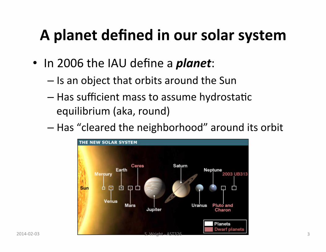
A planet defined in our solar system
• In 2006 the IAU define a planet: – Is an object that orbits around the Sun – Has sufficient mass to assume hydrostaHc equilibrium (aka, round)
– Has “cleared the neighborhood” around its orbit
3 2014-‐02-‐03 S. Wright -‐ AST326
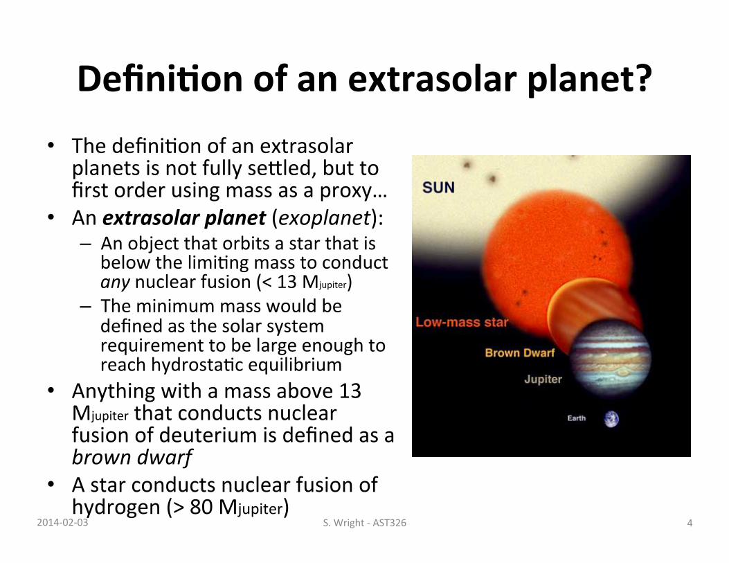
Defini/on of an extrasolar planet? • The definiHon of an extrasolar
planets is not fully seVled, but to first order using mass as a proxy…
• An extrasolar planet (exoplanet): – An object that orbits a star that is below the limiHng mass to conduct any nuclear fusion (< 13 Mjupiter)
– The minimum mass would be defined as the solar system requirement to be large enough to reach hydrostaHc equilibrium
• Anything with a mass above 13 Mjupiter that conducts nuclear fusion of deuterium is defined as a brown dwarf
• A star conducts nuclear fusion of hydrogen (> 80 Mjupiter)
4 2014-‐02-‐03 S. Wright -‐ AST326
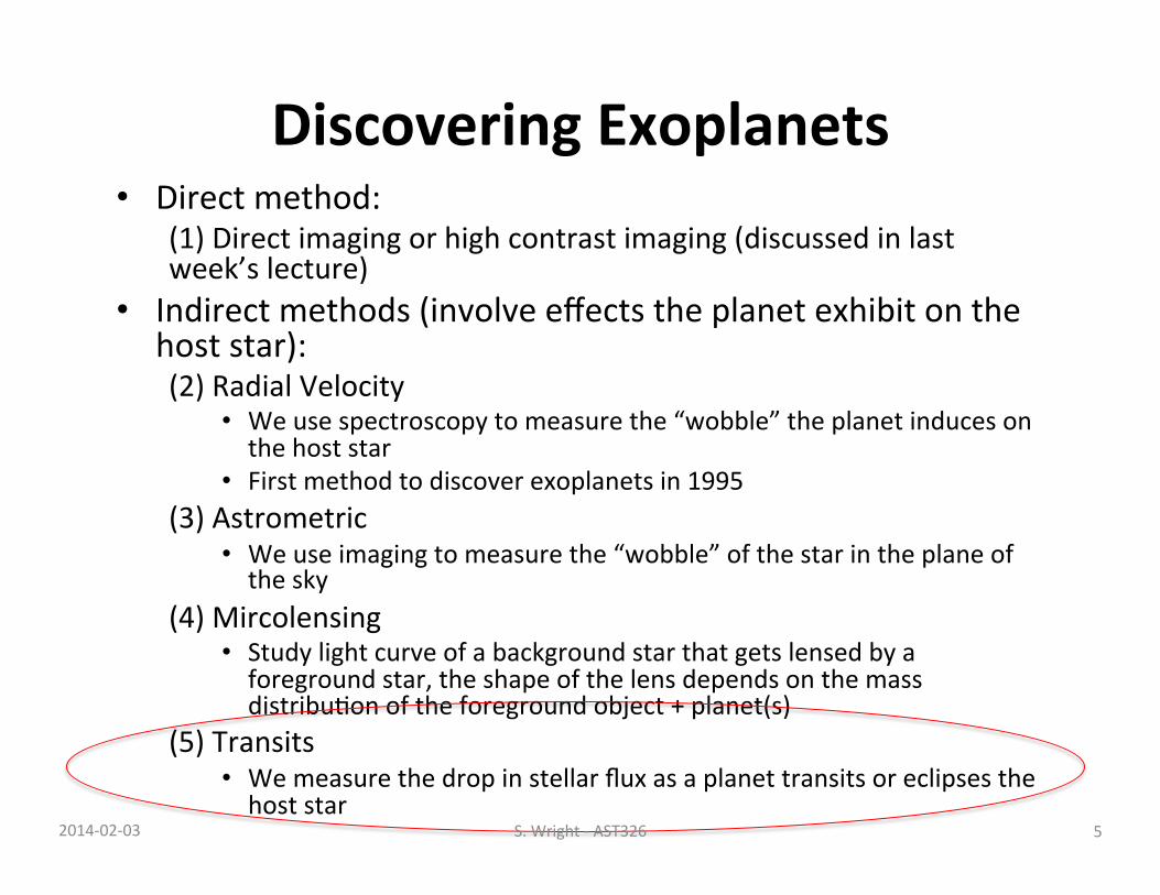
Discovering Exoplanets • Direct method:
(1) Direct imaging or high contrast imaging (discussed in last week’s lecture)
• Indirect methods (involve effects the planet exhibit on the host star): (2) Radial Velocity
• We use spectroscopy to measure the “wobble” the planet induces on the host star
• First method to discover exoplanets in 1995 (3) Astrometric
• We use imaging to measure the “wobble” of the star in the plane of the sky
(4) Mircolensing • Study light curve of a background star that gets lensed by a foreground star, the shape of the lens depends on the mass distribuHon of the foreground object + planet(s)
(5) Transits • We measure the drop in stellar flux as a planet transits or eclipses the host star
5 2014-‐02-‐03 S. Wright -‐ AST326
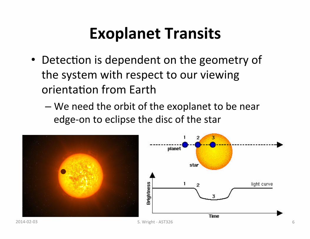
Exoplanet Transits • DetecHon is dependent on the geometry of the system with respect to our viewing orientaHon from Earth – We need the orbit of the exoplanet to be near edge-‐on to eclipse the disc of the star
6 2014-‐02-‐03 S. Wright -‐ AST326
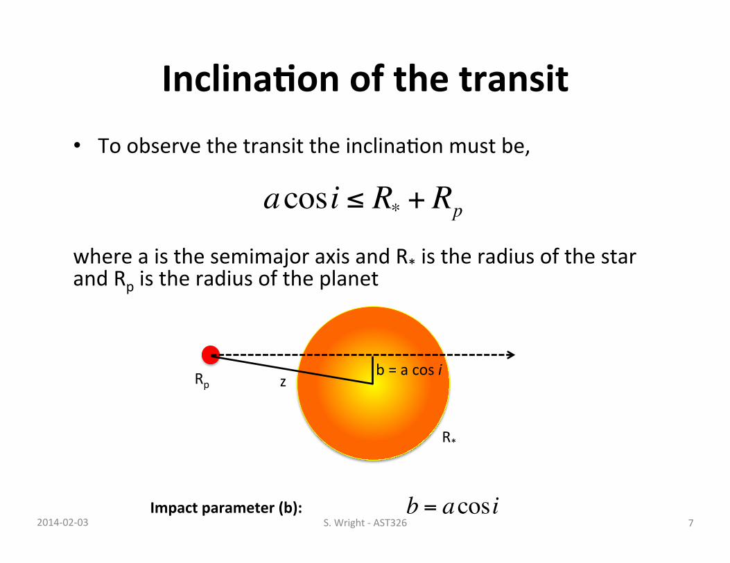
Inclina/on of the transit • To observe the transit the inclinaHon must be,
where a is the semimajor axis and R* is the radius of the star and Rp is the radius of the planet
acosi ≤ R* + Rp
z b = a cos i
b = acosi
R*
Rp
Impact parameter (b): 7 2014-‐02-‐03 S. Wright -‐ AST326
8 2014-‐02-‐03 S. Wright -‐ AST326
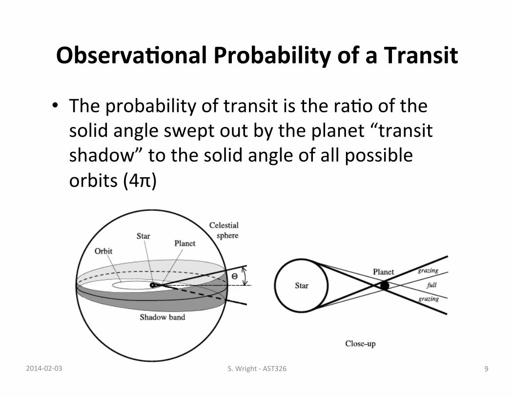
Observa/onal Probability of a Transit
• The probability of transit is the raHo of the solid angle swept out by the planet “transit shadow” to the solid angle of all possible orbits (4π)
9 2014-‐02-‐03 S. Wright -‐ AST326
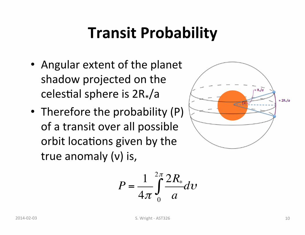
Transit Probability
• Angular extent of the planet shadow projected on the celesHal sphere is 2R*/a
• Therefore the probability (P) of a transit over all possible orbit locaHons given by the true anomaly (ν) is,
P = 14π
2R*a0
2π
∫ dυ
10 2014-‐02-‐03 S. Wright -‐ AST326
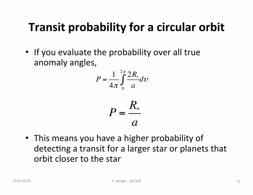
Transit probability for a circular orbit
• If you evaluate the probability over all true anomaly angles,
• This means you have a higher probability of detecHng a transit for a larger star or planets that orbit closer to the star
P = 14π
2R*a0
2π
∫ dυ
P = R*a
11 2014-‐02-‐03 S. Wright -‐ AST326
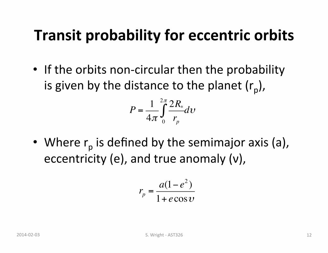
Transit probability for eccentric orbits
• If the orbits non-‐circular then the probability is given by the distance to the planet (rp),
• Where rp is defined by the semimajor axis (a), eccentricity (e), and true anomaly (ν),
P = 14π
2R*rp0
2π
∫ dυ
rp =a(1− e2 )1+ ecosυ
12 2014-‐02-‐03 S. Wright -‐ AST326
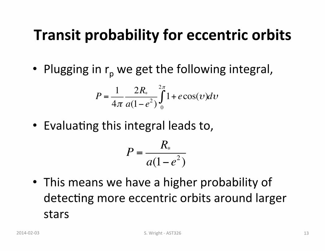
Transit probability for eccentric orbits
• Plugging in rp we get the following integral,
• EvaluaHng this integral leads to,
• This means we have a higher probability of detecHng more eccentric orbits around larger stars
P = 14π
2R*a(1− e2 )
1+ ecos(υ)0
2π
∫ dυ
P = R*a(1− e2 )
13 2014-‐02-‐03 S. Wright -‐ AST326
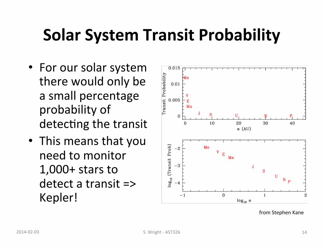
Solar System Transit Probability
• For our solar system there would only be a small percentage probability of detecHng the transit
• This means that you need to monitor 1,000+ stars to detect a transit => Kepler!
from Stephen Kane
14 2014-‐02-‐03 S. Wright -‐ AST326
15 2014-‐02-‐03 S. Wright -‐ AST326
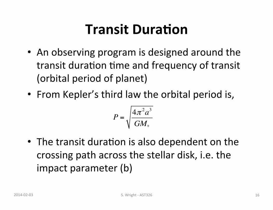
Transit Dura/on • An observing program is designed around the transit duraHon Hme and frequency of transit (orbital period of planet)
• From Kepler’s third law the orbital period is, • The transit duraHon is also dependent on the crossing path across the stellar disk, i.e. the impact parameter (b)
P = 4π 2a3
GM*
16 2014-‐02-‐03 S. Wright -‐ AST326
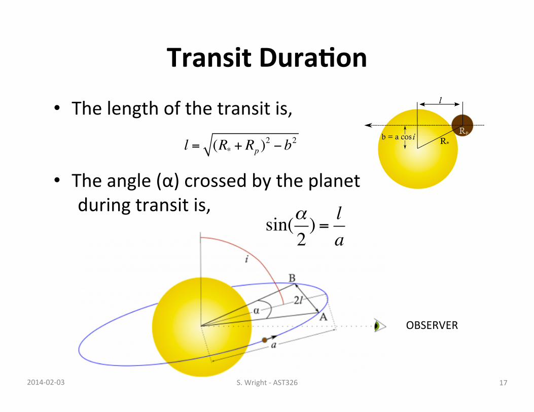
Transit Dura/on
• The length of the transit is,
• The angle (α) crossed by the planet during transit is,
l = (R* + Rp )2 − b2
OBSERVER
sin(α2) = l
a
17 2014-‐02-‐03 S. Wright -‐ AST326
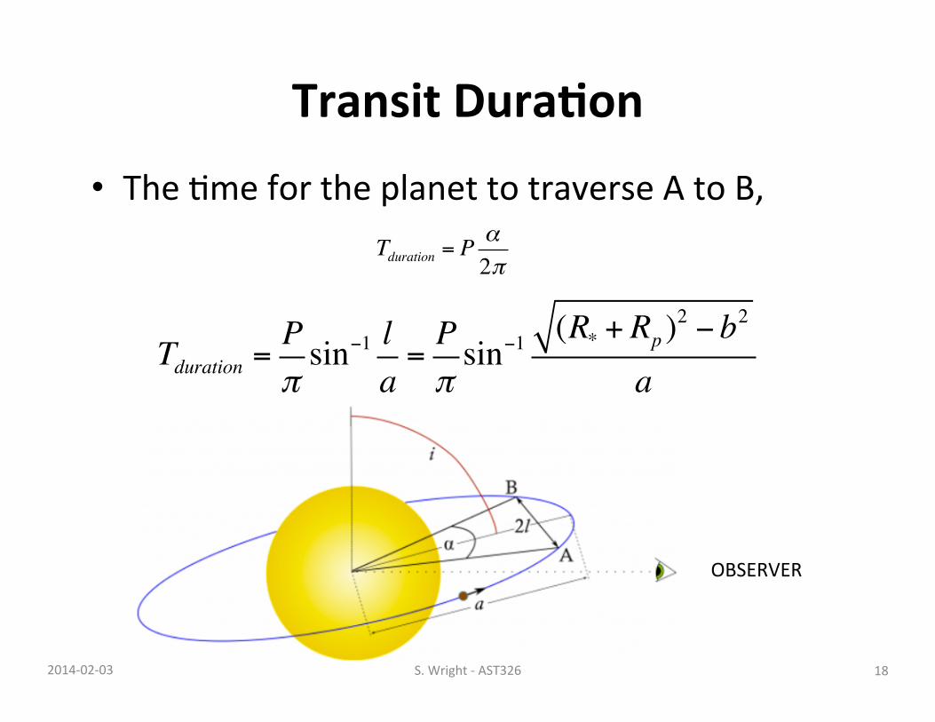
Transit Dura/on
• The Hme for the planet to traverse A to B,
OBSERVER
Tduration = Pα2π
Tduration =Pπsin−1 l
a=Pπsin−1
(R* + Rp )2 − b2
a
18 2014-‐02-‐03 S. Wright -‐ AST326
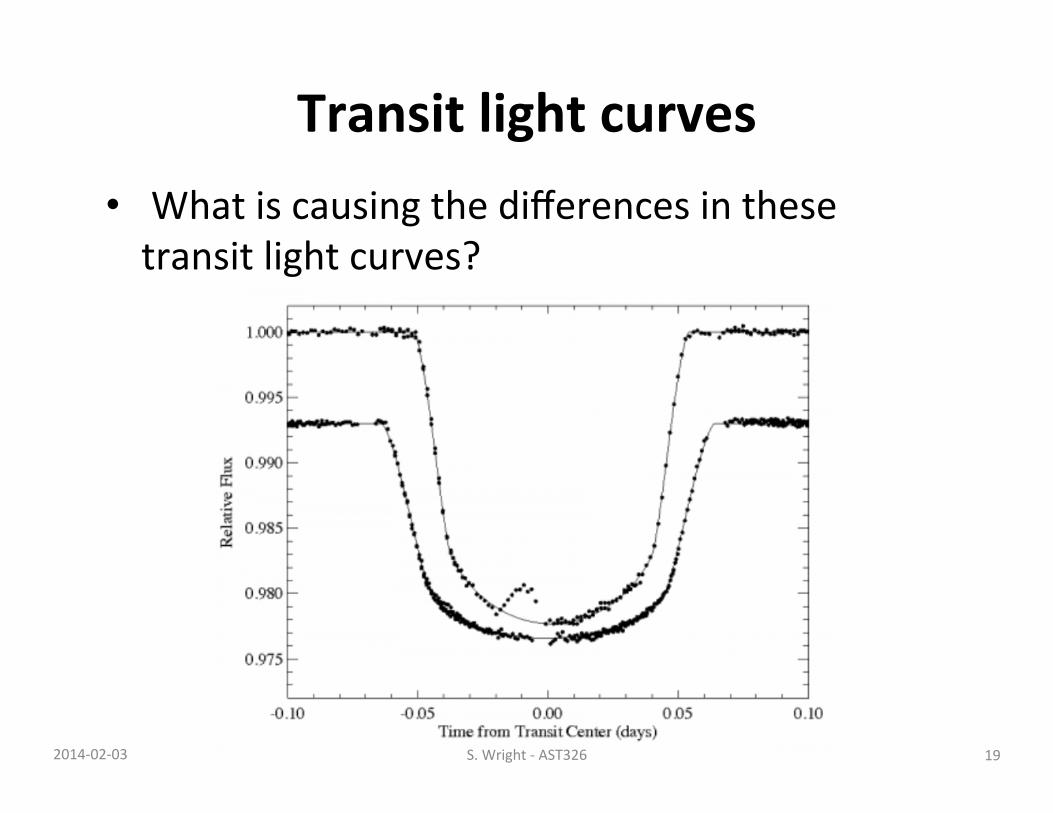
Transit light curves • What is causing the differences in these transit light curves?
19 2014-‐02-‐03 S. Wright -‐ AST326
Principles of photometry
• The light from a star is spread over several pixels non-‐uniformly
• How do we sum the light to get a measure of the total flux from the star? – IdenHfy the locaHon of the star – Select the associated pixels that contain the stellar flux by generaHng a masking region
– Sum up the light • Ensure that the noise and background is not included
20 2014-‐02-‐03 S. Wright -‐ AST326
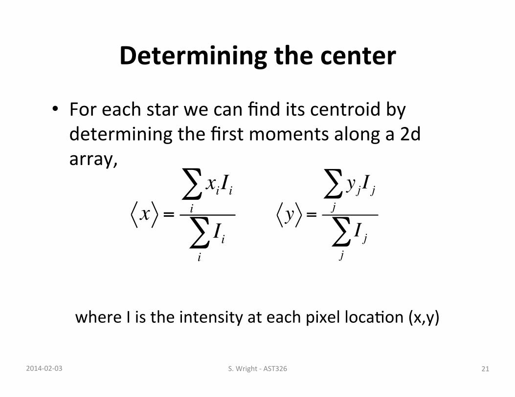
Determining the center
• For each star we can find its centroid by determining the first moments along a 2d array,
where I is the intensity at each pixel locaHon (x,y)
x =xiIi
i∑
Iii∑
y =
yjI jj∑
I jj∑
21 2014-‐02-‐03 S. Wright -‐ AST326
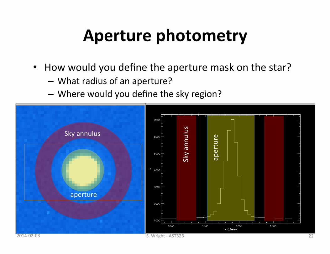
Aperture photometry
• How would you define the aperture mask on the star? – What radius of an aperture? – Where would you define the sky region?
Sky annulus
aperture Sky annu
lus
aperture
22 2014-‐02-‐03 S. Wright -‐ AST326
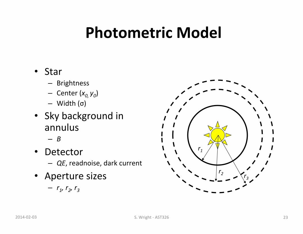
Photometric Model
• Star – Brightness – Center (x0, y0) – Width (σ)
• Sky background in annulus – B
• Detector – QE, readnoise, dark current
• Aperture sizes – r1, r2, r3
r1
r2 r3
23 2014-‐02-‐03 S. Wright -‐ AST326
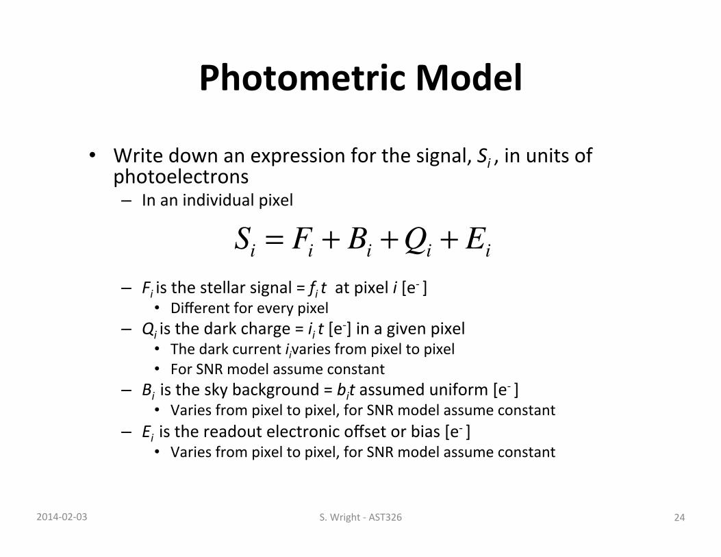
Photometric Model
• Write down an expression for the signal, Si , in units of photoelectrons – In an individual pixel
– Fi is the stellar signal = fi t at pixel i [e-‐ ] • Different for every pixel
– Qi is the dark charge = ii t [e-‐] in a given pixel • The dark current iivaries from pixel to pixel • For SNR model assume constant
– Bi is the sky background = bit assumed uniform [e-‐ ] • Varies from pixel to pixel, for SNR model assume constant
– Ei is the readout electronic offset or bias [e-‐ ] • Varies from pixel to pixel, for SNR model assume constant
�
Si = Fi + Bi +Qi + Ei
24 2014-‐02-‐03 S. Wright -‐ AST326
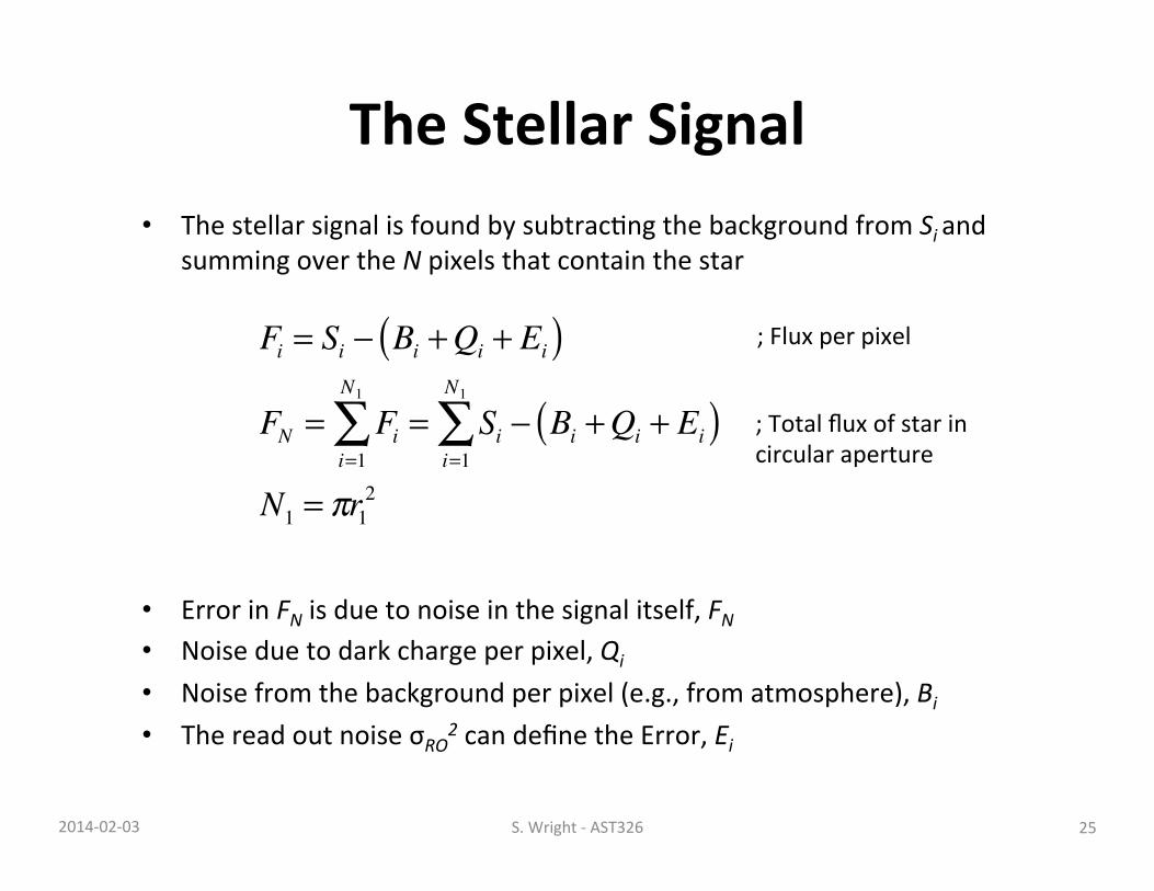
The Stellar Signal • The stellar signal is found by subtracHng the background from Si and
summing over the N pixels that contain the star
• Error in FN is due to noise in the signal itself, FN • Noise due to dark charge per pixel, Qi • Noise from the background per pixel (e.g., from atmosphere), Bi • The read out noise σRO2 can define the Error, Ei
�
Fi = Si − Bi +Qi + Ei( )FN = Fi
i=1
N1
∑ = Si − Bi +Qi + Ei( )i=1
N1
∑N1 = πr1
2
; Flux per pixel
; Total flux of star in circular aperture
25 2014-‐02-‐03 S. Wright -‐ AST326
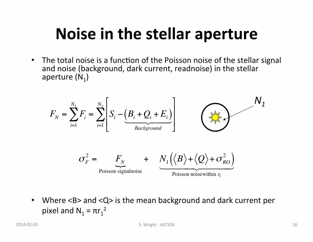
Noise in the stellar aperture • The total noise is a funcHon of the Poisson noise of the stellar signal
and noise (background, dark current, readnoise) in the stellar aperture (N1)
FN = Fii=1
N1
∑ = Si − Bi +Qi +Ei( )Background
#
$
%%
&
'
((i=1
N1
∑N1
• Where <B> and <Q> is the mean background and dark current per pixel and N1 = πr12
σ F2 = FN
Poisson signalnoise + N1 B + Q +σ RO
2( )Poisson noisewithin r1
26 2014-‐02-‐03 S. Wright -‐ AST326
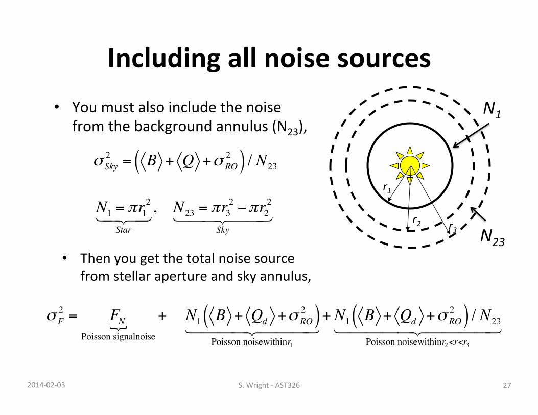
Including all noise sources
σ Sky2 = B + Q +σ RO
2( ) / N23
r1
r2 r3
• You must also include the noise from the background annulus (N23),
N1 = πr12
Star , N23 = πr3
2 −πr22
Sky
σ F2 = FN
Poisson signalnoise + N1 B + Qd +σ RO
2( )Poisson noisewithinr1
+ N1 B + Qd +σ RO
2( ) / N23
Poisson noisewithinr2<r<r3
• Then you get the total noise source from stellar aperture and sky annulus,
N1
N23
27 2014-‐02-‐03 S. Wright -‐ AST326
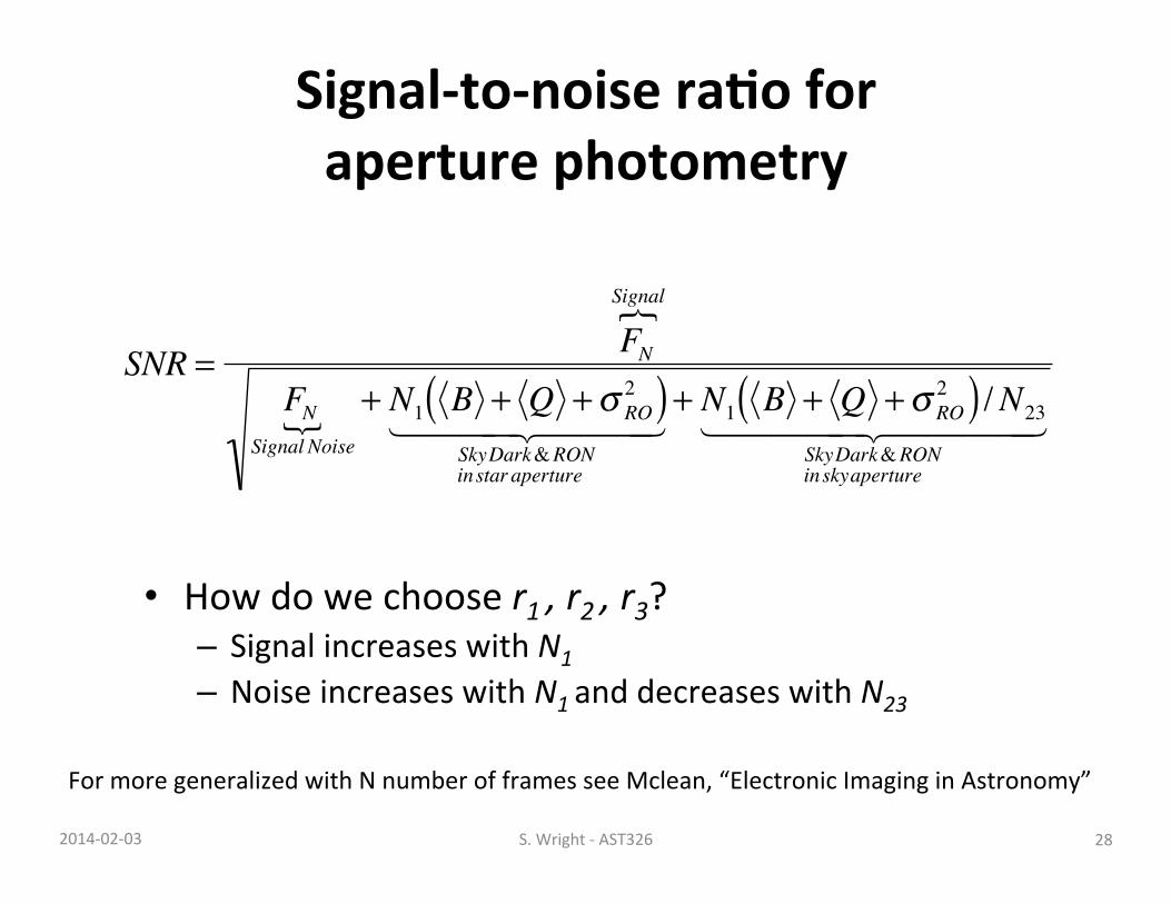
Signal-‐to-‐noise ra/o for aperture photometry
• How do we choose r1 , r2 , r3? – Signal increases with N1 – Noise increases with N1 and decreases with N23
�
SNR =FNSignal
FNSignal Noise + N1 B + Q + σ RO
2( )SkyDark&RONinstar aperture
+ N1 B + Q + σ RO
2( ) /N23
SkyDark&RONinskyaperture
For more generalized with N number of frames see Mclean, “Electronic Imaging in Astronomy”
28 2014-‐02-‐03 S. Wright -‐ AST326
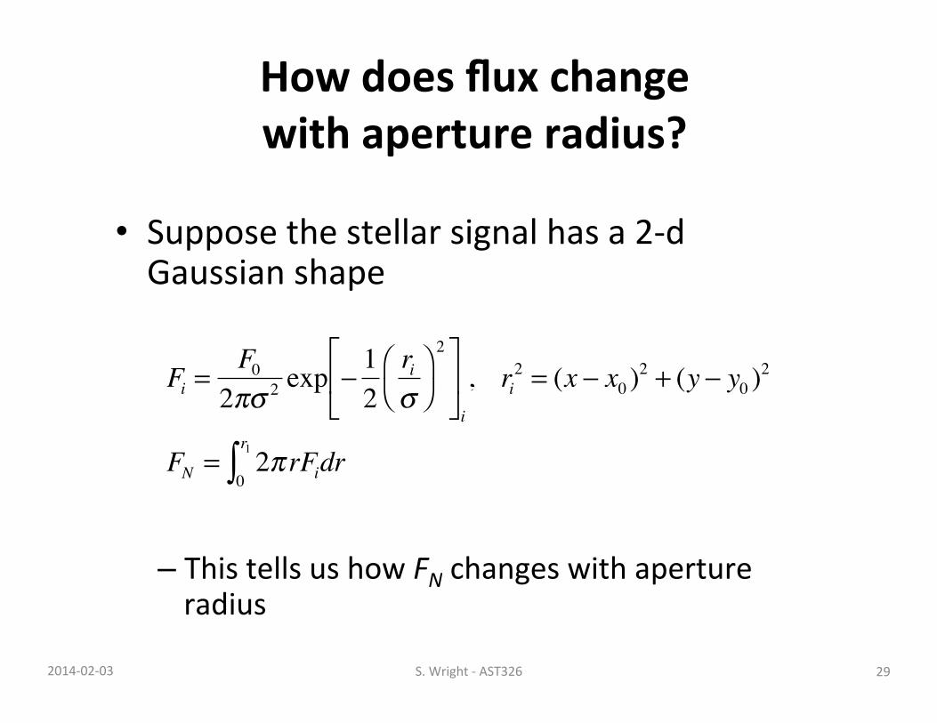
How does flux change with aperture radius?
• Suppose the stellar signal has a 2-‐d Gaussian shape
– This tells us how FN changes with aperture radius �
Fi =F02πσ 2 exp −
12
riσ
⎛ ⎝
⎞ ⎠
2⎡
⎣ ⎢
⎤
⎦ ⎥ i
, ri2 = (x − x0 )
2 + (y − y0 )2
FN = 2π rFi0
r1∫ dr
29 2014-‐02-‐03 S. Wright -‐ AST326
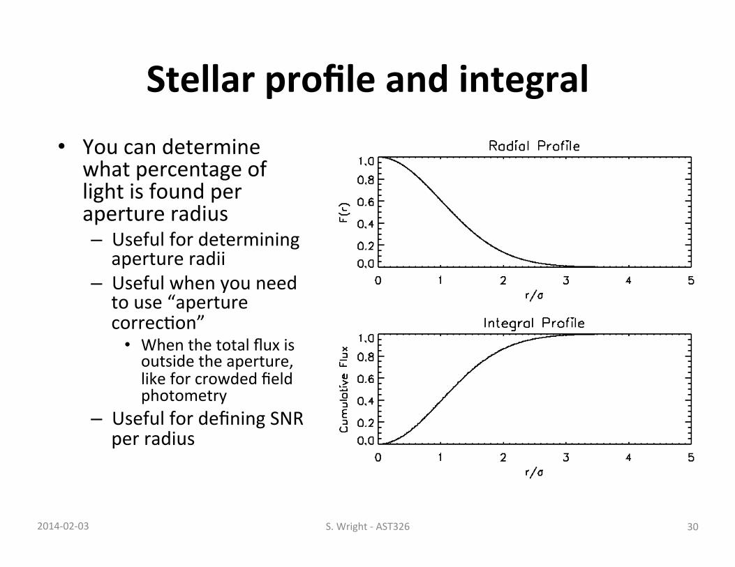
Stellar profile and integral • You can determine
what percentage of light is found per aperture radius – Useful for determining aperture radii
– Useful when you need to use “aperture correcHon” • When the total flux is outside the aperture, like for crowded field photometry
– Useful for defining SNR per radius
30 2014-‐02-‐03 S. Wright -‐ AST326
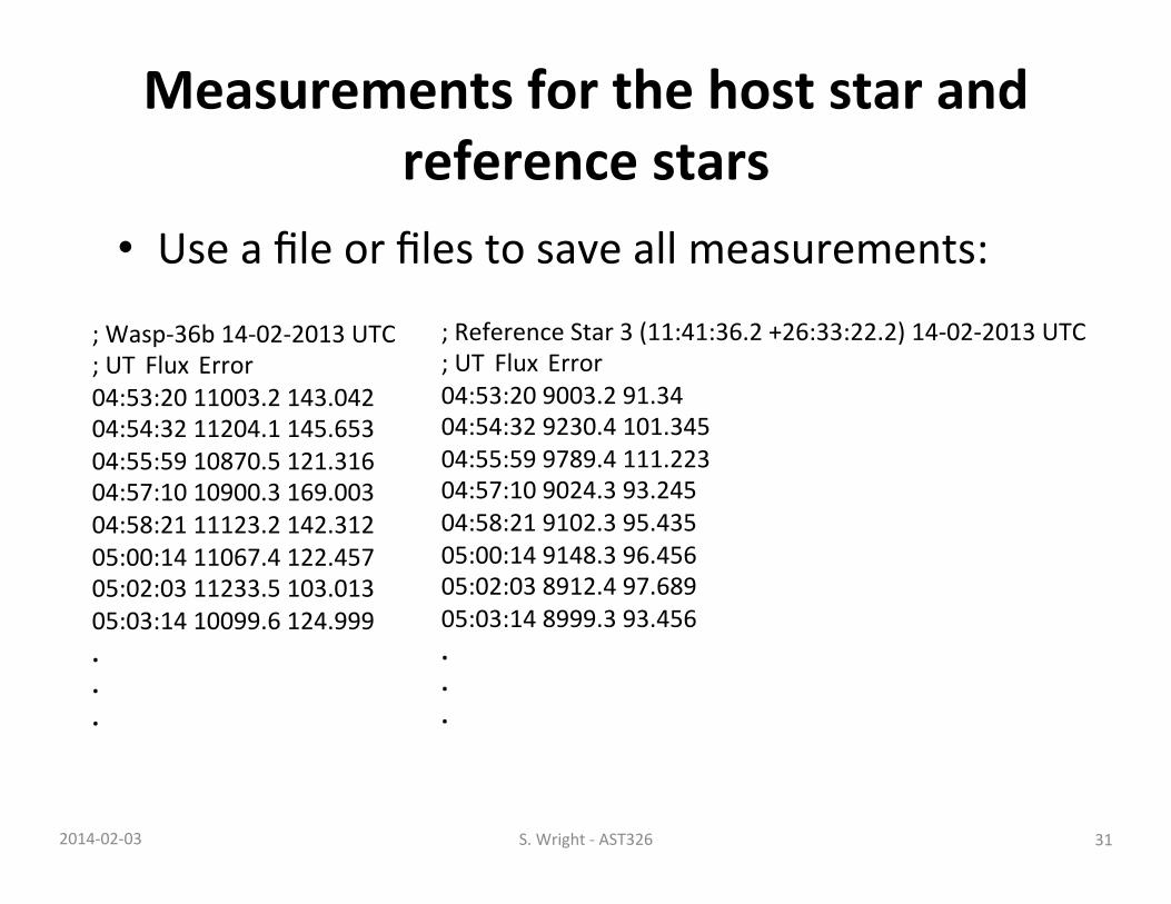
Measurements for the host star and reference stars
• Use a file or files to save all measurements:
; Wasp-‐36b 14-‐02-‐2013 UTC ; UT Flux Error 04:53:20 11003.2 143.042 04:54:32 11204.1 145.653 04:55:59 10870.5 121.316 04:57:10 10900.3 169.003 04:58:21 11123.2 142.312 05:00:14 11067.4 122.457 05:02:03 11233.5 103.013 05:03:14 10099.6 124.999 . . .
; Reference Star 3 (11:41:36.2 +26:33:22.2) 14-‐02-‐2013 UTC ; UT Flux Error 04:53:20 9003.2 91.34 04:54:32 9230.4 101.345 04:55:59 9789.4 111.223 04:57:10 9024.3 93.245 04:58:21 9102.3 95.435 05:00:14 9148.3 96.456 05:02:03 8912.4 97.689 05:03:14 8999.3 93.456 . . .
31 2014-‐02-‐03 S. Wright -‐ AST326
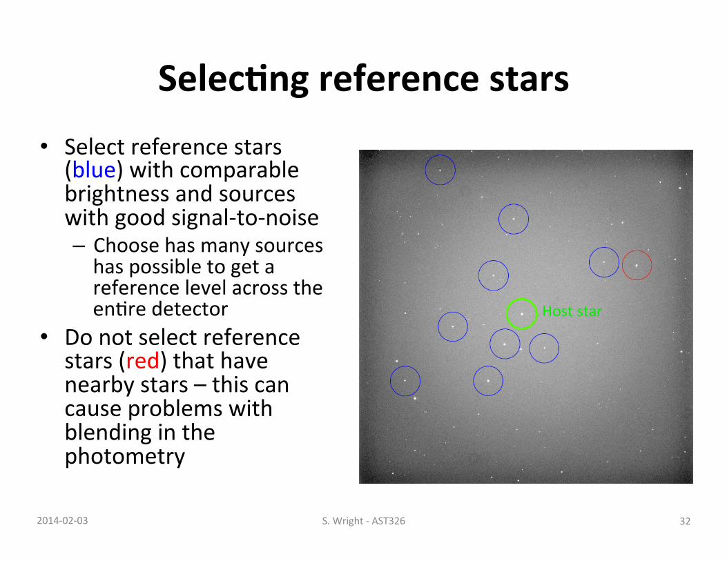
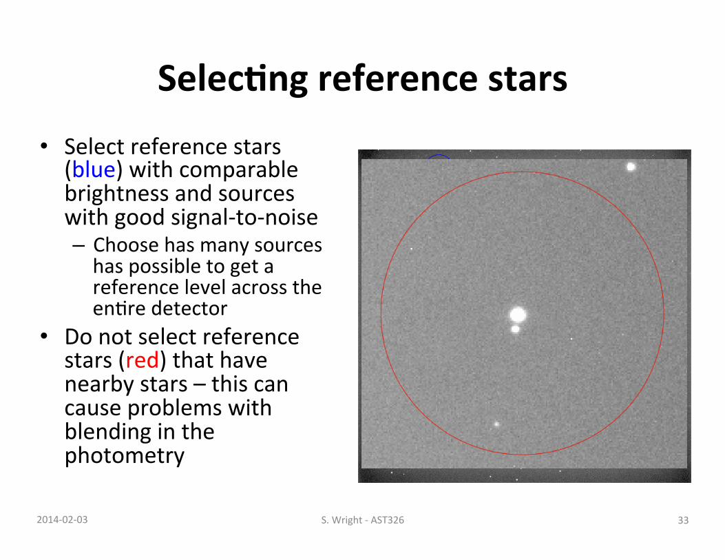
Selec/ng reference stars • Select reference stars (blue) with comparable brightness and sources with good signal-‐to-‐noise – Choose has many sources has possible to get a reference level across the enHre detector
• Do not select reference stars (red) that have nearby stars – this can cause problems with blending in the photometry
Host star
32 2014-‐02-‐03 S. Wright -‐ AST326
Selec/ng reference stars • Select reference stars (blue) with comparable brightness and sources with good signal-‐to-‐noise – Choose has many sources has possible to get a reference level across the enHre detector
• Do not select reference stars (red) that have nearby stars – this can cause problems with blending in the photometry
Host star
33 2014-‐02-‐03 S. Wright -‐ AST326
Weighted average of reference stars
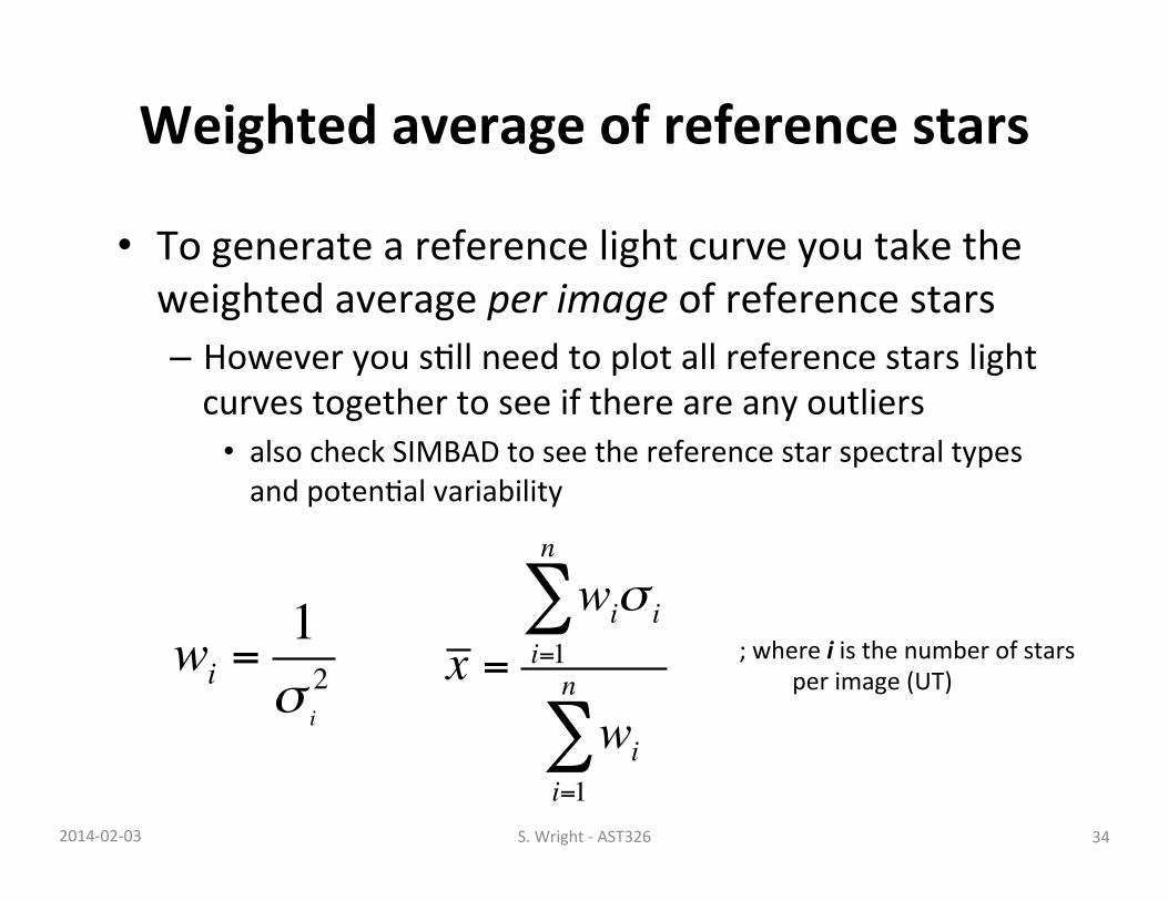
• To generate a reference light curve you take the weighted average per image of reference stars – However you sHll need to plot all reference stars light curves together to see if there are any outliers • also check SIMBAD to see the reference star spectral types and potenHal variability
wi =1σ i2 x =
wiσ ii=1
n
∑
wii=1
n
∑; where i is the number of stars
per image (UT)
34 2014-‐02-‐03 S. Wright -‐ AST326
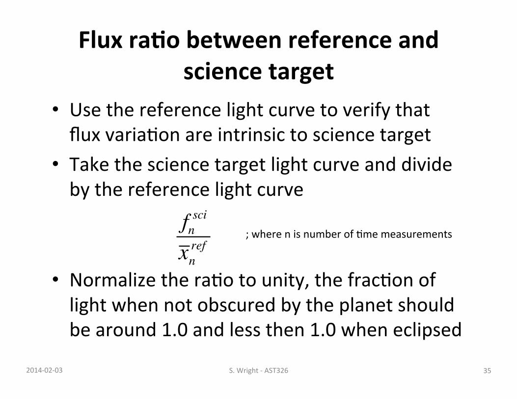
Flux ra/o between reference and science target
• Use the reference light curve to verify that flux variaHon are intrinsic to science target
• Take the science target light curve and divide by the reference light curve
• Normalize the raHo to unity, the fracHon of light when not obscured by the planet should be around 1.0 and less then 1.0 when eclipsed
fnsci
xnref
; where n is number of Hme measurements
35 2014-‐02-‐03 S. Wright -‐ AST326
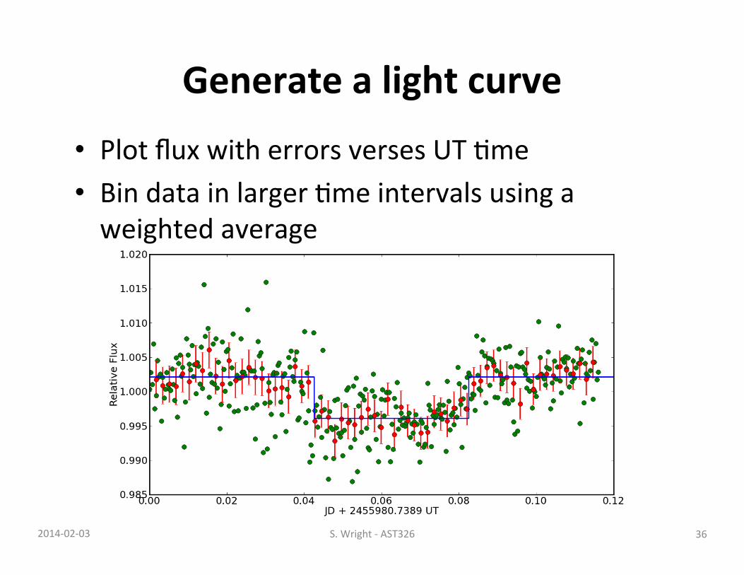
Generate a light curve
• Plot flux with errors verses UT Hme • Bin data in larger Hme intervals using a weighted average
36 2014-‐02-‐03 S. Wright -‐ AST326
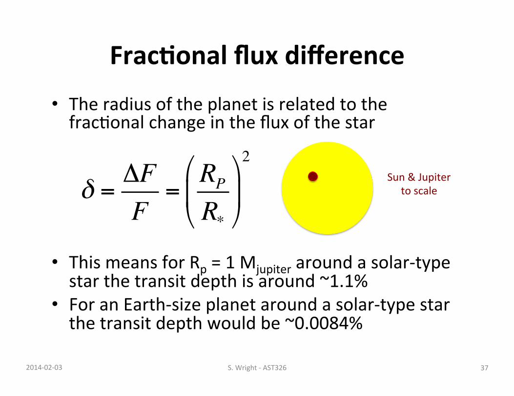
Frac/onal flux difference
• The radius of the planet is related to the fracHonal change in the flux of the star
• This means for Rp = 1 Mjupiter around a solar-‐type star the transit depth is around ~1.1%
• For an Earth-‐size planet around a solar-‐type star the transit depth would be ~0.0084%
δ =ΔFF
=RPR*
"
#$
%
&'
2Sun & Jupiter
to scale
37 2014-‐02-‐03 S. Wright -‐ AST326
Proper/es from transit light curves
• Transit depth yields the radius of planet (Rp) • DuraHon of transit and ingress yields the inclinaHon (i) and (with monitoring) the period of orbit (P)
• Since the inclinaHon is constrained you can esHmate the mass of the planet (Mp)
• Given the mass of the planet you can esHmate the density of the planet (ρp)
• The shape of the boVom of the light curve can be used to fit limb darkening
38 2014-‐02-‐03 S. Wright -‐ AST326
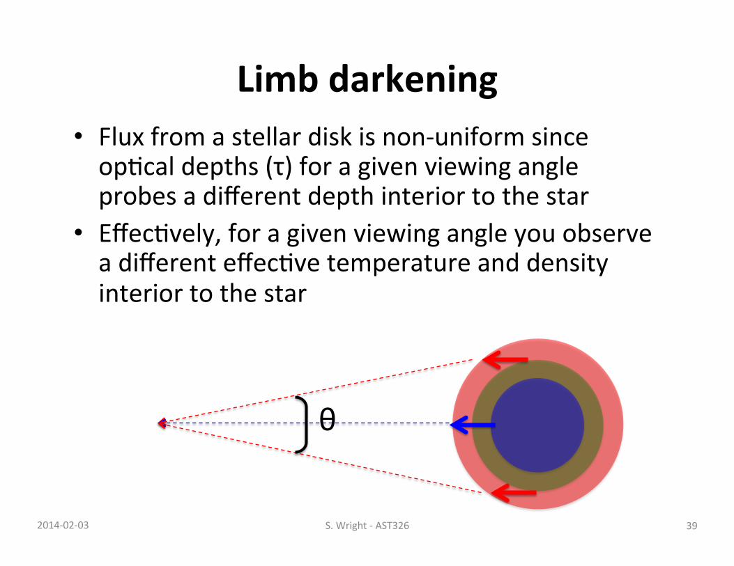
Limb darkening • Flux from a stellar disk is non-‐uniform since opHcal depths (τ) for a given viewing angle probes a different depth interior to the star
• EffecHvely, for a given viewing angle you observe a different effecHve temperature and density interior to the star
θ
39 2014-‐02-‐03 S. Wright -‐ AST326
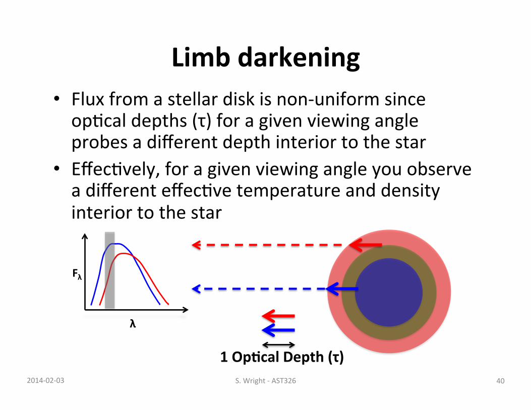
Limb darkening • Flux from a stellar disk is non-‐uniform since opHcal depths (τ) for a given viewing angle probes a different depth interior to the star
• EffecHvely, for a given viewing angle you observe a different effecHve temperature and density interior to the star
1 Op/cal Depth (τ)
λ
Fλ
40 2014-‐02-‐03 S. Wright -‐ AST326
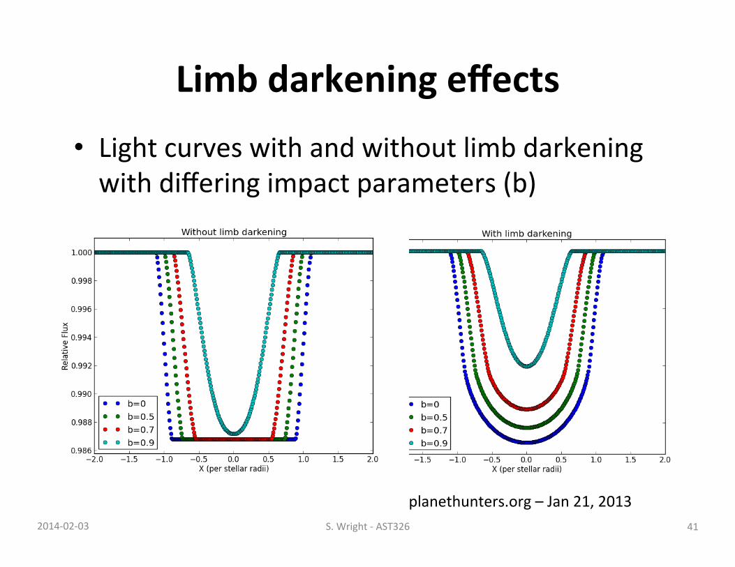
Limb darkening effects
planethunters.org – Jan 21, 2013
• Light curves with and without limb darkening with differing impact parameters (b)
41 2014-‐02-‐03 S. Wright -‐ AST326
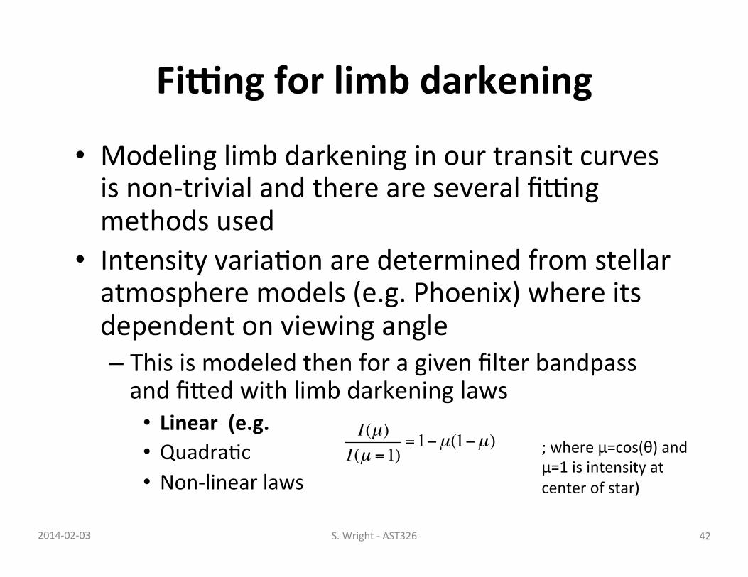
FiWng for limb darkening
• Modeling limb darkening in our transit curves is non-‐trivial and there are several fi�ng methods used
• Intensity variaHon are determined from stellar atmosphere models (e.g. Phoenix) where its dependent on viewing angle – This is modeled then for a given filter bandpass and fiVed with limb darkening laws • Linear (e.g. • QuadraHc • Non-‐linear laws
I(µ)I(µ =1)
=1−µ(1−µ) ; where μ=cos(θ) and μ=1 is intensity at center of star)
42 2014-‐02-‐03 S. Wright -‐ AST326
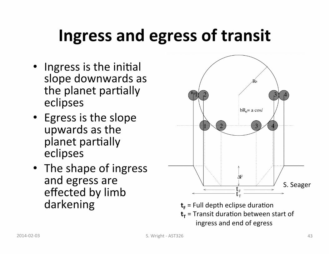
Ingress and egress of transit
• Ingress is the iniHal slope downwards as the planet parHally eclipses
• Egress is the slope upwards as the planet parHally eclipses
• The shape of ingress and egress are effected by limb darkening
S. Seager
tF = Full depth eclipse duraHon tT = Transit duraHon between start of
ingress and end of egress
43 2014-‐02-‐03 S. Wright -‐ AST326
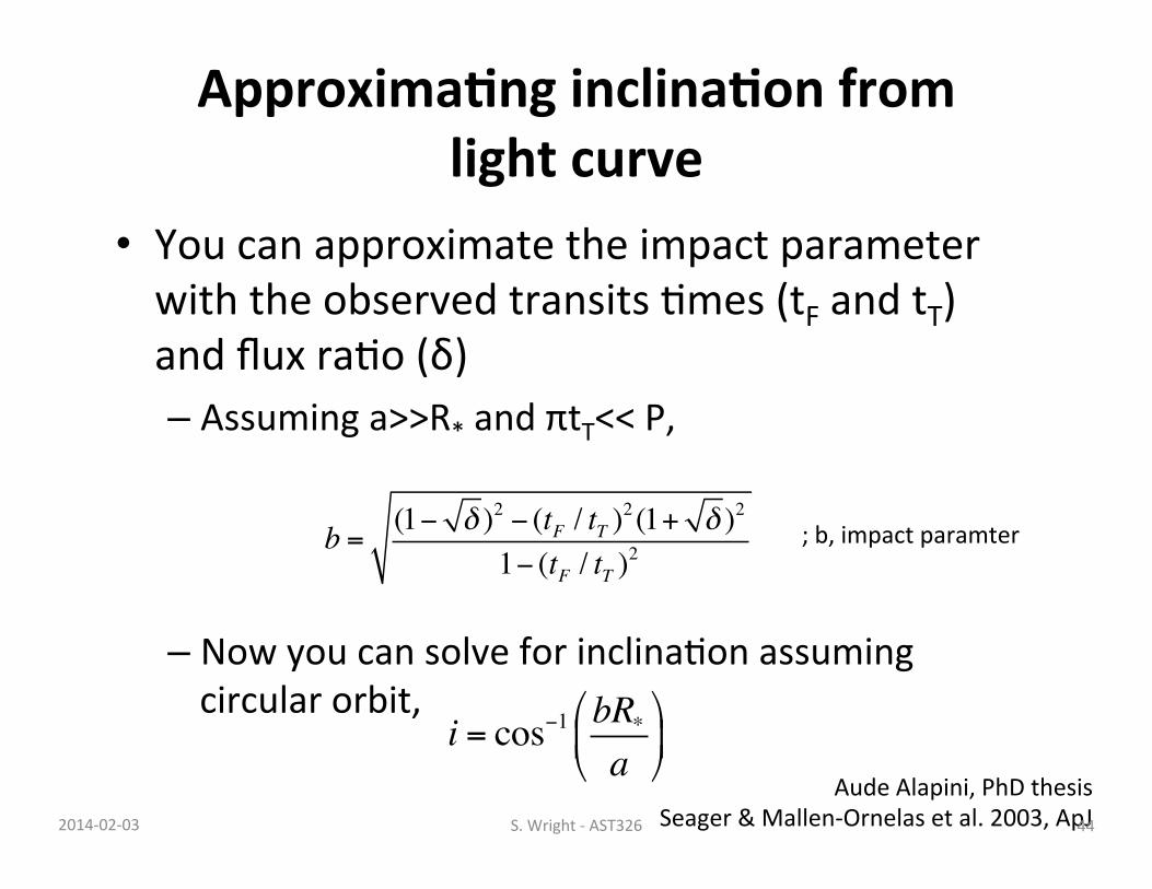
Approxima/ng inclina/on from light curve
• You can approximate the impact parameter with the observed transits Hmes (tF and tT) and flux raHo (δ) – Assuming a>>R* and πtT<< P,
– Now you can solve for inclinaHon assuming circular orbit,
b = (1− δ )2 − (tF / tT )2 (1+ δ )2
1− (tF / tT )2
; b, impact paramter
i = cos−1 bR*a
"
#$
%
&'
Aude Alapini, PhD thesis Seager & Mallen-‐Ornelas et al. 2003, ApJ 44 2014-‐02-‐03 S. Wright -‐ AST326
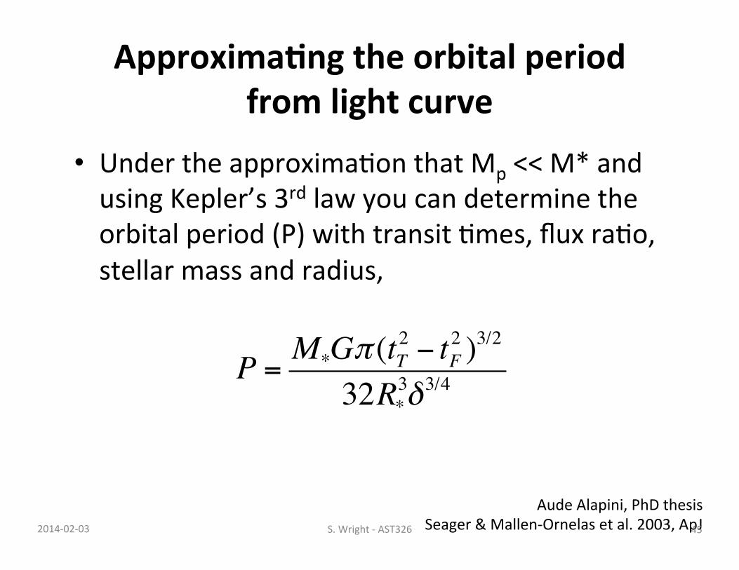
Approxima/ng the orbital period from light curve
• Under the approximaHon that Mp << M* and using Kepler’s 3rd law you can determine the orbital period (P) with transit Hmes, flux raHo, stellar mass and radius,
Aude Alapini, PhD thesis Seager & Mallen-‐Ornelas et al. 2003, ApJ
P = M*Gπ (tT2 − tF
2 )3/2
32R*3δ3/4
45 2014-‐02-‐03 S. Wright -‐ AST326
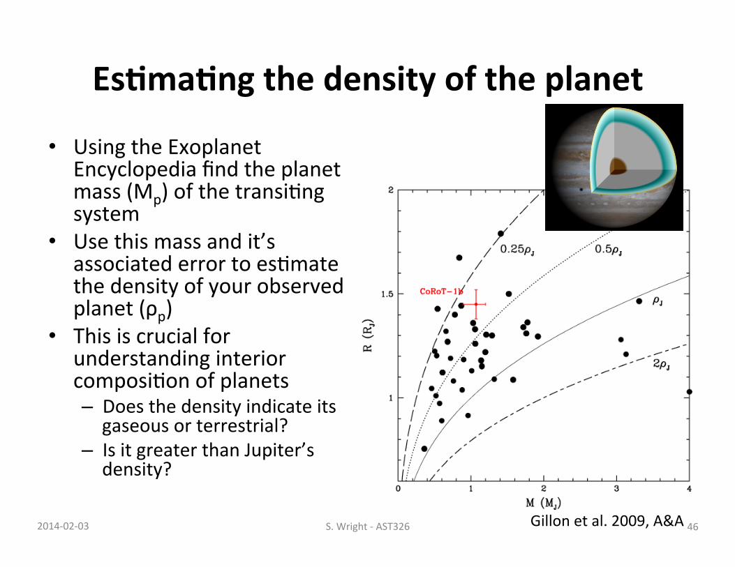
Es/ma/ng the density of the planet
• Using the Exoplanet Encyclopedia find the planet mass (Mp) of the transiHng system
• Use this mass and it’s associated error to esHmate the density of your observed planet (ρp)
• This is crucial for understanding interior composiHon of planets – Does the density indicate its gaseous or terrestrial?
– Is it greater than Jupiter’s density?
Gillon et al. 2009, A&A 46 2014-‐02-‐03 S. Wright -‐ AST326
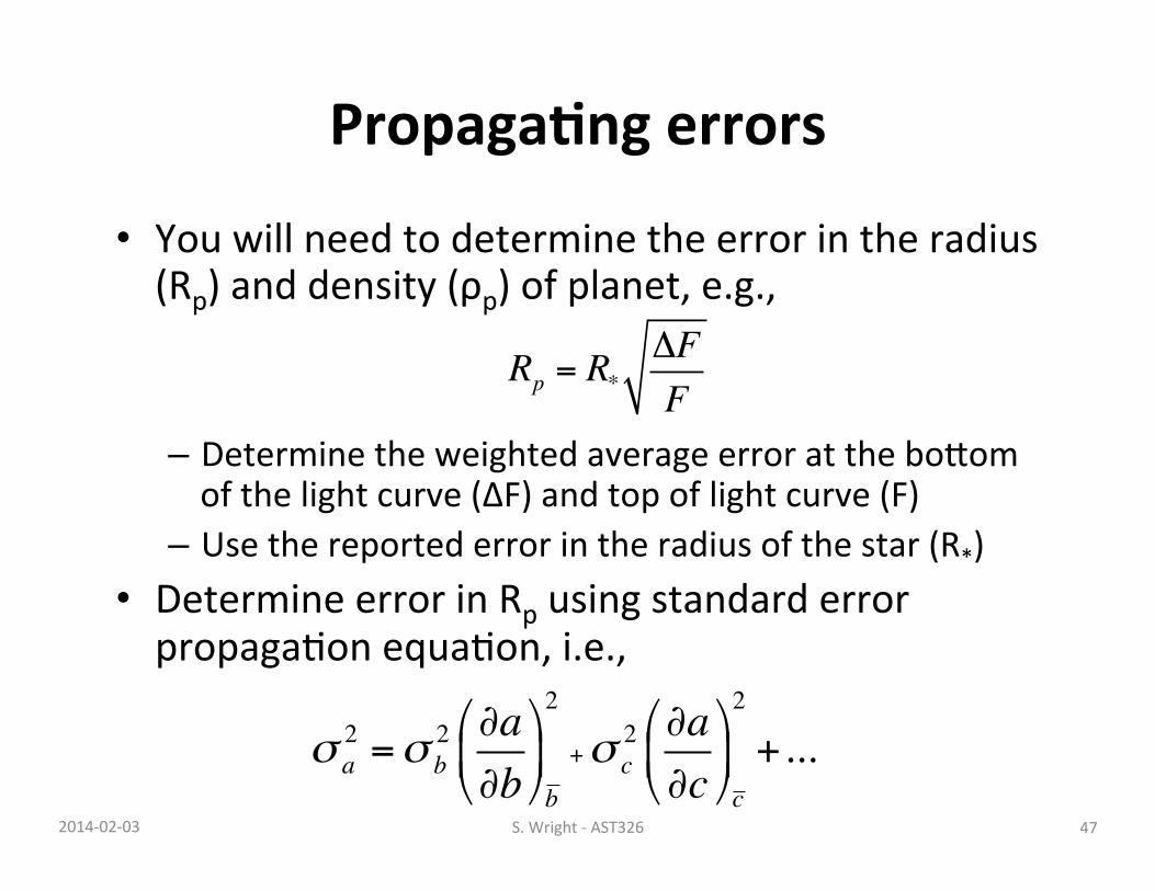
Propaga/ng errors
• You will need to determine the error in the radius (Rp) and density (ρp) of planet, e.g.,
– Determine the weighted average error at the boVom of the light curve (ΔF) and top of light curve (F)
– Use the reported error in the radius of the star (R*) • Determine error in Rp using standard error propagaHon equaHon, i.e.,
σ a2 =σ b
2 ∂a∂b"
#$
%
&'b
2
+σ c2 ∂a∂c"
#$
%
&'c
2
+...
Rp = R*ΔFF
47 2014-‐02-‐03 S. Wright -‐ AST326