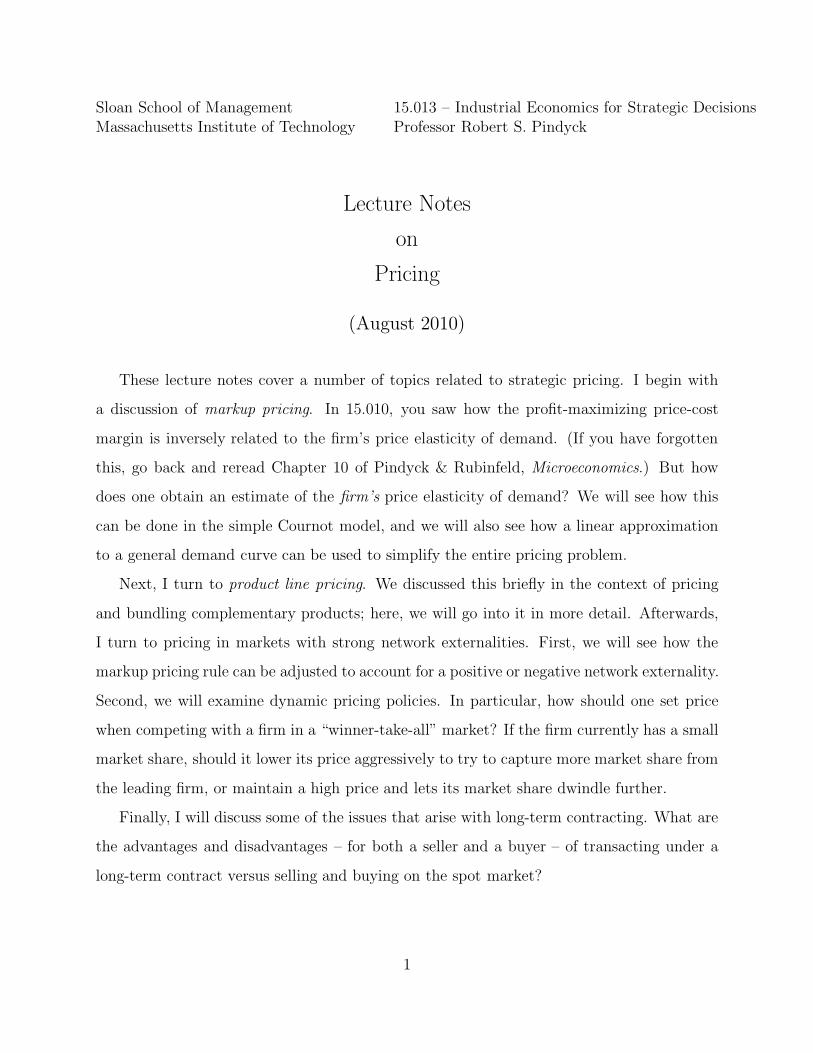
Sloan School of Management 15.013 – Industrial Economics for Strategic DecisionsMassachusetts Institute of Technology Professor Robert S. Pindyck

Lecture Notes

on

Pricing

(August 2010)

These lecture notes cover a number of topics related to strategic pricing. I begin with

a discussion of markup pricing. In 15.010, you saw how the profit-maximizing price-cost

margin is inversely related to the firm’s price elasticity of demand. (If you have forgotten

this, go back and reread Chapter 10 of Pindyck & Rubinfeld, Microeconomics.) But how

does one obtain an estimate of the firm’s price elasticity of demand? We will see how this

can be done in the simple Cournot model, and we will also see how a linear approximation

to a general demand curve can be used to simplify the entire pricing problem.

Next, I turn to product line pricing. We discussed this briefly in the context of pricing

and bundling complementary products; here, we will go into it in more detail. Afterwards,

I turn to pricing in markets with strong network externalities. First, we will see how the

markup pricing rule can be adjusted to account for a positive or negative network externality.

Second, we will examine dynamic pricing policies. In particular, how should one set price

when competing with a firm in a “winner-take-all” market? If the firm currently has a small

market share, should it lower its price aggressively to try to capture more market share from

the leading firm, or maintain a high price and lets its market share dwindle further.

Finally, I will discuss some of the issues that arise with long-term contracting. What are

the advantages and disadvantages – for both a seller and a buyer – of transacting under a

long-term contract versus selling and buying on the spot market?

1

1 Markup Pricing

In 15.010, you saw that profit maximization implies that marginal revenue should equal

marginal cost, which in turn implies:

P − MC

P= −

1

Ed(1)

Here, Ed, is the firm’s price elasticity of demand. Note that this equation can be rewritten

as:

P =MC

1 + (1/Ed)(2)

If the firm is a monopolist, then the relevant elasticity is the market elasticity of demand,

which I will denote by ED. Obtaining an estimate of this market elasticity of demand may

or may not be difficult, but for the moment, let’s assume that we have such an estimate.

Given this estimate of ED, how can we obtain an estimate of the firm’s price elasticity of

demand, Ed.

1.1 Cournot Competition

If we assume that the firms in the market compete a la Cournot (which may or may not

be a reasonable assumption), obtaining the elasticity of demand for an individual firm is

fairly straightforward. Suppose that there are n equal-sized firms in the market, and that

they all have the same marginal cost, c. In the Cournot model, each firm chooses its profit-

maximizing output taking the outputs of its competitors as fixed.

For Firm i, profit is given by:

Πi = [P (Q)− c]Qi (3)

where Q is the total output of the industry. We want to maximize this profit with respect

to Qi, treating the Qj’s for the other firms as fixed:

∂Πi

∂Qi= P (Q) − c + Qi

dP

dQ

∂Q

∂Qi= 0 (4)

Note that dQ/dQi = 1, and dQj/dQi = 0. Thus, the reaction curve for Firm i is:

P (Q) + QidP

dQ= c (5)

2

Because there are n equal-sized firms, we know that Qi = Q/n. Thus eqn. (5) becomes:

P (Q) +Q

n

dP

dQ= c (6)

If we divide both sides of this equation by P and rearrange the terms, we get:

P − c

P= −

1

n

Q

P

dP

dQ= −

1

nED(7)

Compare this result to eqn. (1). Note that:

Ed = nED (8)

Thus, with n equal sized firms, going from the market elasticity of demand to the firm’s

elasticity of demand is quite easy: just multiply the market elasticity by n.

There are very few markets in which all of the firms are the same size. Suppose that

instead we have m firms of unequal size. As long as the assumption of Cournot competition

holds, obtaining the elasticity of demand for each firm is still straightforward. I will not

go through the details (you can try to derive this as an exercise), but the procedure is as

follows:

First, calculate the Herfindahl-Hirschman index (HHI) for the industry:

HHI =m∑

i=1

S2i , (9)

where Si is the market share of Firm i.

Next, find n∗, the equivalent number of equal-sized firms that yields the same value of

the HHI calculated above. In other words, find n∗ such that:

n∗∑

i=1

(1/n∗)2 = n∗(1/n∗)2 = 1/n∗ = HHI (10)

Thus, n∗ is simply the reciprocal of the HHI, i.e., n∗ = 1/HHI. Now, just use this n∗ to

obtain Ed:

Ed = n∗ED (11)

Suppose, for example, that there are four firms with market shares of 40%, 30%, 15%, and

15% respectively. In that case, the HHI is given by: HHI = (.4)2+(.3)2+(.15)2+(.15)2 = .295.

Thus, n∗ = 1/.295 = 3.39, and Ed = 3.39ED.

3

Earlier in the course, we applied these results to the market for beer. You might recall

that for mass market beers (Budweiser, Miller, etc.), the market elasticity of demand has

been shown from statistical studies to be about -0.8. Recall that competition in attribute

space is local, i.e., a particular brand only competes with its nearby neighbors in the attribute

space. For mass market beer, this local competition implies a value of n (or n∗) of about

four or five. Thus, for a typical mass market brand of beer, the elasticity of demand is

approximately Ed = (5)(−.8) = −4.0. Using eqn. (2), this means that the profit maximizing

price is roughly:

P = MC1−(1/4)

= 1.33MC

(Remember that this is a wholesale price.) We can see from this that profit-maximizing price-

cost markups for mass market beer are likely to be fairly small. This means that aggressive

price competition can be extremely damaging, which, as we discussed, is one reason that

firms prefer to compete aggressively using advertising rather than price.

We know that in many industries firms use price as a strategic variable, rather than

quantity. Recall that the use of price rather than quantity as a strategic variable intensifies

competition and reduces profits. (If you don’t remember this, go back and review the Lecture

Notes on Game Theory.) This means that the effective elasticity of demand for a particular

brand is likely to be larger in magnitude than the Cournot model would predict. But how

much larger? That depends on the cross-price elasticities among the different brands.

If the cross-price elasticities are large (i.e., the brands are fairly close substitutes), the

Cournot analysis won’t work: Ed is likely to be much larger than nED. If, on the other

hand, substitutability among brands is limited, our Cournot result will likely still hold.

In what kinds of markets is our oligopoly markup rule likely to work, and in what kinds

of markets will it not work? It will work in markets where competition is fairly stable, and

involves choices of output and/or capacity. One example that we have studied in depth is

beer, where the major firms try to avoid price competition, and focus instead on advertising.

It will also work in markets for automobiles (where firms choose capacity, which makes the

4

outcome similar to Cournot). Likewise, it is likely to work in markets for mineral resources

(copper, aluminum) and some service industries (such as shipping and insurance).

The oligopoly markup rule is unlikely to work, however, in markets where competition

and pricing are dynamic in nature, and where strategic multi-period gaming is important.

We discuss this below.

1.2 Strategic Considerations

Remember that the Cournot model is essentially static; it assumes that each firm takes the

output of its competitors as fixed. As explained above, this assumption is quite reasonable

for the large number of markets where competition is stable and dynamic price wars are

generally avoided. As we have seen throughout this course, this kind of stable pricing could

arise if the same firms having been competing for a long time (and there is little prospect

of entry by new firms), production cost and market demand conditions are relatively stable,

and the firms face a repeated Prisoners’ Dilemma with no end point (and thus little or no

likelihood of “unravelling”). But the Cournot assumption will not be reasonable for markets

where pricing and output decisions are dominated by dynamic gaming considerations.

Airlines. One example is airlines, where very low short-run marginal costs result in

intense price competition, particularly for certain fare categories. As you have seen, airline

pricing is also complicated by the fact that prices are linked to yield management (i.e., the

allocation, which changes from day to day, of the number of seats for each fare category).

What can an airline do to avoid the intense price competition that is so prevalent in the

industry? As we have discussed, one strategy is seek and maintain “monopoly routes,” where

it is the only airline to offer non-stop service.

Retail Store Pricing. Retail store pricing is in many ways similar to the Strategic

Oligopoly Game that you play every week — it is repeated Prisoners’ Dilemma with a fixed

end point. You know that in this kind of repeated game, “unravelling” is likely to occur. That

is exactly what happens to retail store pricing each year during November and December.

The last play of the retail store repeated game occurs on December 24. Price competition

becomes intense well before that date as stores face the unhappy prospect of being stuck

5

with large amounts of unsold inventories that they will have to dump, often at below cost.

Over the years, managers of large retail chains and department stores have become in-

creasingly sophisticated in their understanding of game theory. What has this done for

them? The result is that they are more aware of the unravelling problem, and they are

aware that their competitors are also aware of the problem. Thus they anticipate that the

unravelling will start earlier. Not wanting to be the “sucker” who gets undercut and winds

up with lots of unsold inventories, each store tries to get a jump on the unravelling. And

as you would expect, the unravelling starts earlier. Ten years ago the unravelling generally

began on or just after Thanksgiving, five years ago in mid-November, and in more recent

years unravelling has started by the beginning of November.

If you ran a retail store chain, how should you go about setting prices? First of all, you

are stuck in a bad place and deserve a lot of sympathy! Beyond that, the best you can do

try to predict when and how the unravelling is likely to occur, make sure you are not on

vacation or asleep when it starts, and take it into account when you determine the quantities

that you will purchase at wholesale.

Commercial Aircraft. Finally, one more more example of an industry in which pricing

is dominated by gaming and bargaining is commercial aircraft. As we have discussed at

length in this course, the durable goods monopoly problem, combined with the ability of

airlines to play Boeing and Airbus off against each other, can drive prices down toward

marginal cost.

2 The Linear Demand Approximation

A nice thing about industries such as beer, soft drinks, breakfast cereals, airlines, auto-

mobiles, etc., is that they have been around for a long time, and a good deal of data are

available so that we can estimate market demand curves. Often, however, firms must set

the prices of new products for which there is little or no history of demand or consumer

response to price changes. You saw an example of this early in this course when we studied

the emerging market for Internet music downloads and the pricing problem facing Apple.

6

How might managers think about pricing in such situations?

Suppose that you were trying to set the price of a prescription drug such as Prilosec

(an antiulcer medication). You would know that Prilosec competes with other proton-pump

inhibitor antiulcer drugs such as Prevacid and Nexium, as well as the earlier generation

H2-antagonist antiulcer drugs such as Zantac, Pepcid, and Axid. You would also know

that marginal production cost is quite low. However, you might find it difficult to estimate

the elasticity of demand for the drug. Rather than try to estimate the elasticity of demand

directly, an alternative approach is to approximate the demand curve as linear. In particular,

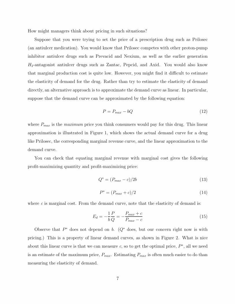
suppose that the demand curve can be approximated by the following equation:

P = Pmax − bQ (12)

where Pmax is the maximum price you think consumers would pay for this drug. This linear

approximation is illustrated in Figure 1, which shows the actual demand curve for a drug

like Prilosec, the corresponding marginal revenue curve, and the linear approximation to the

demand curve.

You can check that equating marginal revenue with marginal cost gives the following

profit-maximizing quantity and profit-maximizing price:

Q∗ = (Pmax − c)/2b (13)

P ∗ = (Pmax + c)/2 (14)

where c is marginal cost. From the demand curve, note that the elasticity of demand is:

Ed = −

1

b

P

Q= −

Pmax + c

Pmax − c(15)

Observe that P ∗ does not depend on b. (Q∗ does, but our concern right now is with

pricing.) This is a property of linear demand curves, as shown in Figure 2. What is nice

about this linear curve is that we can measure c, so to get the optimal price, P ∗, all we need

is an estimate of the maximum price, Pmax. Estimating Pmax is often much easier to do than

measuring the elasticity of demand.

7

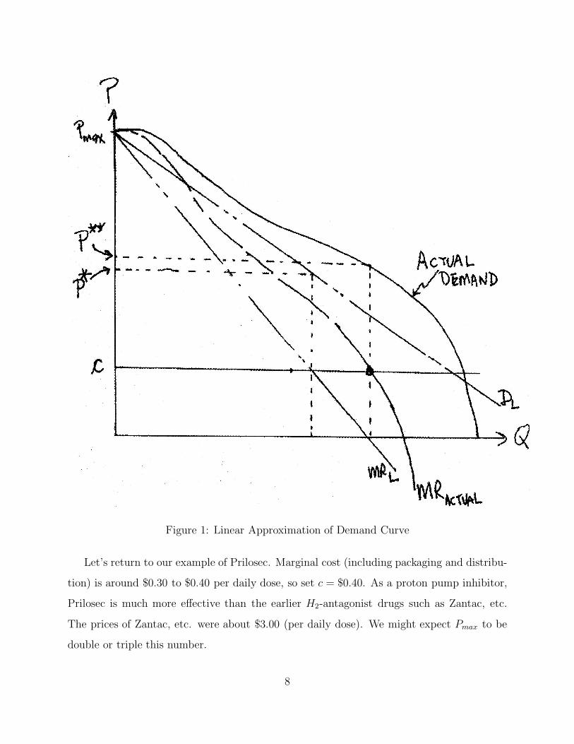
Figure 1: Linear Approximation of Demand Curve

Let’s return to our example of Prilosec. Marginal cost (including packaging and distribu-

tion) is around $0.30 to $0.40 per daily dose, so set c = $0.40. As a proton pump inhibitor,

Prilosec is much more effective than the earlier H2-antagonist drugs such as Zantac, etc.

The prices of Zantac, etc. were about $3.00 (per daily dose). We might expect Pmax to be

double or triple this number.

8

Figure 2: Linear Demand Curves

If Pmax = $9.00, P ∗ = $9.40/2 = $4.70, which implies that the elasticity of demand

is Ed = −(9.40)/(8.60) = −1.09. On the other hand, if Pmax = $6.00, this implies that

P ∗ = $3.20, so that the elasticity of demand is −1.14. Taking an average of these two

demand elasticities suggests that Ed = −1.12 is a good estimate. This, in turn, implies that

the optimal price should be roughly P ∗ = 0.40/(1 − 1/1.12) = $3.73. This is indeed close to

the actual price that was charged for Prilosec.1

1Prilosec was introduced by Astra-Merck in 1995. The pricing of Prilosec is discussed in Example 10.1 of

Pindyck and Rubinfeld, Microeconomics.

9

To take one more example, consider Gillette’s pricing of the Mach 3 razor. Gillette has a

large market share, but still faces some competition from Schick and others. What might be

a reasonable estimate of the maximum price that people would pay for this razor? Given the

prices of other razors (including Gillette’s Sensor), a good estimate would probably be in the

range of $8 to $12. Given that the marginal cost of production and distribution is $4, this

implies a profit-maximizing price in the range of $6.00 to $8.00. When Gillette introduced

the Mach 3 in 1998, they priced it to sell at retail for $6.49 to $6.99.

3 Product Line Pricing

When a firm produces two or more products that have interrelated demands (i.e., they are

substitutes or complements), to maximize profits the firm must price the products jointly,

not individually. The reason is that this enables the firm to internalize the effects of sales of

each product on the sales of the other products.

You saw this earlier when we studied the bundling of complementary products. (Recall

that complements are goods that tend to be used together, e.g., a computer operating system

and applications software that runs on that operating system.) You saw that when two

products are complements, a firm that produces both of them (e.g., the operating system

and the applications software) should set lower prices than would two independent firms,

each of which sells just one of the products. We saw that, in some cases, the firm would

want to sell one of the products at a price that was below its marginal cost, or even a price

that was zero or negative. (If all of this seems a bit hazy, go back and review the Lecture

Notes on Bundling and Brand Proliferation, Section 1.)

Now, let’s consider a case in which a firm sells two products that are substitutes. For

example: (i) a supermarket sells gourmet foods and staples, (ii) Embraer sells the 80-seat

Model 175 and the 100-seat Model 190 passenger jets. For simplicity, we will assume that

the demand curves are linear:

Q1 = a0 − P1 + .5P2 (16)

Q2 = b0 + .5P1 − P2 (17)

10

We will assume that the marginal cost for both products is the same and equal to the

constant c.

3.1 Pricing the Products Individually

Suppose the firm sets prices individually, i.e., suppose it sets P1 to maximize Π1, and sets

P2 to maximize Π2. The resulting prices are found as follows.

Π1 = (P1 − c)Q1 (18)

set ∂Π1/∂P1 = 0 and get:

P1 = (a0 + c)/2 +1

4P2 (19)

Likewise, setting ∂Π2/∂P2 = 0, we get

P2 = (b0 + c)/2 +1

4P1 (20)

Combining these equations for P1 and P2, we find that the optimal prices are:

P1 = (8a0 + 2b0 + 10c)/15 (21)

P2 = (8b0 + 2a0 + 10c)/15 (22)

These prices are the same as those that would result if the two products were produced by

separate firms, each taking its competitor’s price into account, yielding a Nash equilibrium in

prices. The reason is that the single firm producing both products is treating each product

individually and ignoring the fact that it can internalize the demand spillover from one

product to another.

Suppose that a0 = 100, b0 = 50, c = 10. Then P1 = $66.70, P2 = $46.70, Q1 = 56.60,

Q2 = 36.6, and ΠT = $4, 552.40.

3.2 Pricing the Products Jointly

Now suppose that instead, the firm sets the prices of the two products jointly, i.e., it sets P1

and P2 to maximize total profit, ΠT :

ΠT = (P1 − c)Q1 + (P2 − c)Q2 (23)

11

To maximize this, set ∂ΠT/∂P1 = 0 to get:

P1 = (a0 + .5c)/2 +1

2P2 (24)

Likewise, set ∂ΠT/∂P2 = 0 and get:

P2 = (b0 + .5c)/2 +1

2P1 (25)

Combining these two equations, we find that the optimal prices are:

P1 = (2a0 + b0 + 1.5c)/3 (26)

P2 = (2b0 + a0 + 1.5c)/3 (27)

Using the same parameter values, i.e., a0 = 100, b0 = 50, and c = 10, we have P1 = $88.30,

P2 = $71.70, Q1 = 47.3, Q2 = 22.5, and ΠT = $5, 088.80. Note that now the prices are higher,

and total profit ΠT is also higher. Why? The reason is that the higher price for each product

stimulates the sale of the other product, and the firm is taking this into account.

3.3 More General Demand Curves

Obtaining the profit-maximizing prices is straightforward when the demand curves are linear,

as in our example above, but how can those prices be found for more general demand curves?

Consider the general demand curves Q1 = Q1(P1, P2) and Q2 = Q2(P1, P2). Once again,

write down the expression for total profit, and then maximize this with respect to P1 and P2

by setting the derivatives with respect to each price equal to 0. You can check that doing

that yields the following two equations:

P1 + (P1 − c)E11 + (P2 − c)(Q2/Q1)E21 = 0 (28)

P2 + (P2 − c)E22 + (P1 − c)(Q1/Q2)E12 = 0 (29)

where E11 and E22 are own-price elasticities (< 0), and E21 and E12 are cross-price elasticities

(> 0 if the products are substitutes, < 0 if the products are complements). In principle,

these two equations can be solved (probably numerically) for the two prices P1 and P2.

12

We can get some insight into how the prices should be set without actually solving these

two equations numerically. Consider Product 1. Rearranging the first equation yields:

P1 =c

1 + 1/E11−

(P2 − c)(Q2/Q1)E21/E11

1 + 1/E11(30)

The first term on the right-hand side of this equation is the standard markup. The second

term is an adjustment for the impact of P1 on the sales of Product 2. We can determine

this adjustment using estimates of our expected profit margin for Product 2 (as a substitute

for P2 − c), the relative sales volumes (Q2/Q1), and the “relative elasticity” E21/E11. Note

that if E21 > 0, i.e., the products are substitutes, the adjustment raises P1, but if E21 < 0,

it lowers P1.

4 Pricing with Network Externalities

When the demand for a product is subject to network externalities, pricing becomes some-

what more complicated. First, in a static context, the presence of a network externality

affects the elasticity of demand for the product. As you have seen before, a positive network

externality makes demand more elastic, and a negative network externality makes it less

elastic. At issue is how one can take this into account when setting price.

In a dynamic context, a strong positive network externality can complicate price setting.

Suppose you face a single competitor in what is likely to be a “winner-take-all” market.

If you and your competitor are just starting out, should you set your price very low in

order to become the “winner,” even if this means losing a great deal of money in the short

run. And if you do, how would you expect your competitor to respond? Alternatively,

suppose that you have been in the market for some time, but have only a 30% market share,

compared to your competitor’s 70% share. Should you sharply undercut your competitor

in an attempt to increase your market share (and eventually overtake your competitor), or

should you simply maintain a high price, knowing that your market share will eventually

dwindle toward zero? We will examine both the static and dynamic aspects of pricing. We

will begin by considering a simple adjustment to the markup pricing rule that can account

for the presence of a network externality, at least in static terms.

13

4.1 Static Pricing

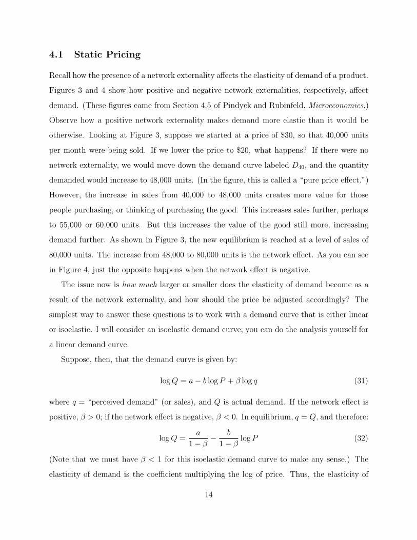
Recall how the presence of a network externality affects the elasticity of demand of a product.

Figures 3 and 4 show how positive and negative network externalities, respectively, affect

demand. (These figures came from Section 4.5 of Pindyck and Rubinfeld, Microeconomics.)

Observe how a positive network externality makes demand more elastic than it would be

otherwise. Looking at Figure 3, suppose we started at a price of $30, so that 40,000 units

per month were being sold. If we lower the price to $20, what happens? If there were no

network externality, we would move down the demand curve labeled D40, and the quantity

demanded would increase to 48,000 units. (In the figure, this is called a “pure price effect.”)

However, the increase in sales from 40,000 to 48,000 units creates more value for those

people purchasing, or thinking of purchasing the good. This increases sales further, perhaps

to 55,000 or 60,000 units. But this increases the value of the good still more, increasing

demand further. As shown in Figure 3, the new equilibrium is reached at a level of sales of

80,000 units. The increase from 48,000 to 80,000 units is the network effect. As you can see

in Figure 4, just the opposite happens when the network effect is negative.

The issue now is how much larger or smaller does the elasticity of demand become as a

result of the network externality, and how should the price be adjusted accordingly? The

simplest way to answer these questions is to work with a demand curve that is either linear

or isoelastic. I will consider an isoelastic demand curve; you can do the analysis yourself for

a linear demand curve.

Suppose, then, that the demand curve is given by:

log Q = a − b log P + β log q (31)

where q = “perceived demand” (or sales), and Q is actual demand. If the network effect is

positive, β > 0; if the network effect is negative, β < 0. In equilibrium, q = Q, and therefore:

log Q =a

1 − β−

b

1 − βlog P (32)

(Note that we must have β < 1 for this isoelastic demand curve to make any sense.) The

elasticity of demand is the coefficient multiplying the log of price. Thus, the elasticity of

14

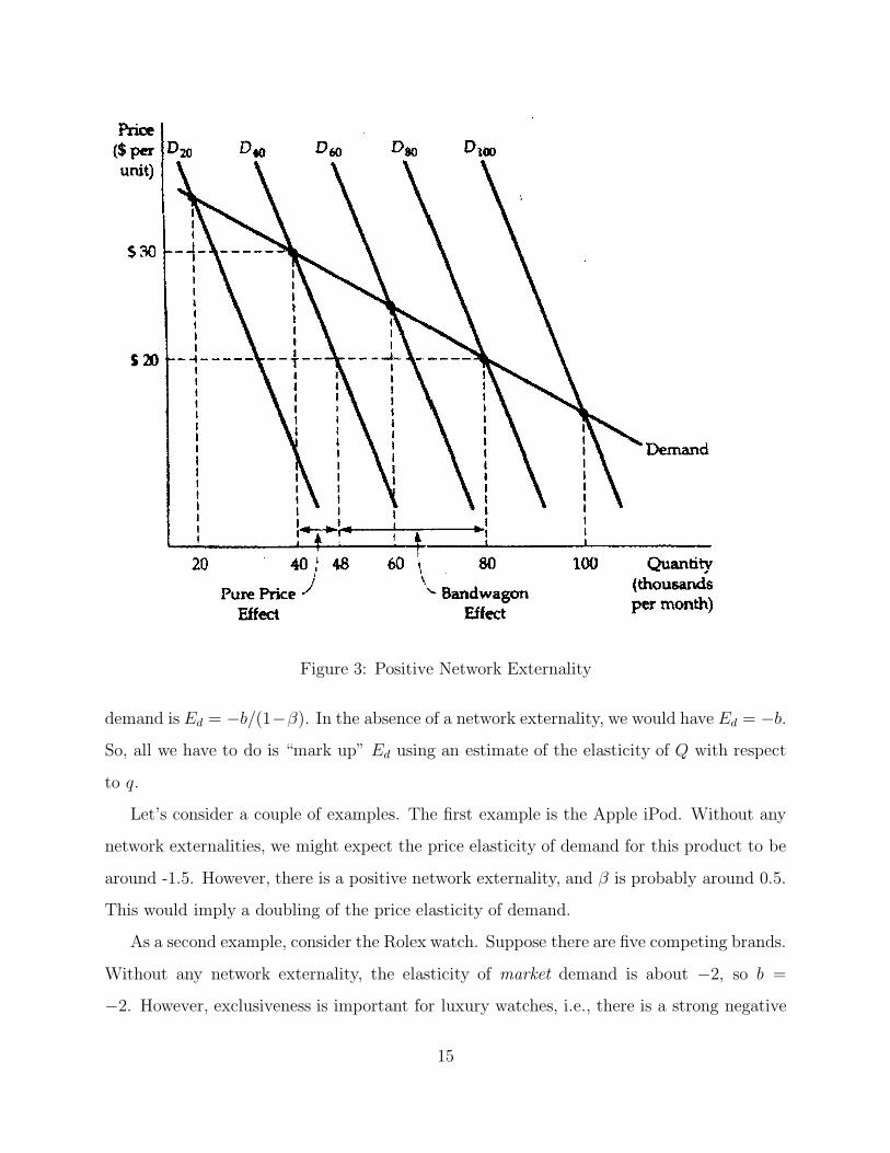
Figure 3: Positive Network Externality

demand is Ed = −b/(1−β). In the absence of a network externality, we would have Ed = −b.

So, all we have to do is “mark up” Ed using an estimate of the elasticity of Q with respect

to q.

Let’s consider a couple of examples. The first example is the Apple iPod. Without any

network externalities, we might expect the price elasticity of demand for this product to be

around -1.5. However, there is a positive network externality, and β is probably around 0.5.

This would imply a doubling of the price elasticity of demand.

As a second example, consider the Rolex watch. Suppose there are five competing brands.

Without any network externality, the elasticity of market demand is about −2, so b =

−2. However, exclusiveness is important for luxury watches, i.e., there is a strong negative

15

Figure 4: Negative Network Externality

network externality. Perhaps, β = −10 (so that a 1% increase in q results in a 10% decrease

in Q). Then, the elasticity of market demand is ED = −2/11, or about −0.2. However,

n = 5, so the brand elasticity is Ed = (5)(−0.2) = −1. Thus, P should be much, much

higher than marginal cost, which, in fact, it is.

4.2 Dynamic Pricing

Dynamic pricing applies to situations in which firms have competing “networks,” and there

is a process of saturation. Each firm wants its consumers to use its “network,” rather than

16

the “network” of its competitor. Because of the positive network externality, the greater the

share of consumers that a firm has, the easier it is to attract additional consumers. Each

firm can affect the rate at which it attracts consumers by altering its price and/or its level

of advertising. However, as the market saturates, a firm with a small market share will find

it very difficult to attract additional consumers, even if it lowers its price substantially.

A much-cited example of this kind of competition was the battle over VHS versus Beta

in videocassette recorders, in which the VHS “network” eventually won. Other examples

include Microsoft Word versus Word Perfect in word processing software, Microsoft’s Win-

dows versus IBM’s OS/2 in desktop operating systems, the Apple iPod (which stores music

in a proprietary format) versus competing MP3 music players, and PDAs using the Palm

operating system versus those using Windows CE.

Suppose that you are competing against another firm, and both of you are starting with

small but equal numbers of consumers using your “networks.” Should you price aggressively

in order to “win” the market, or should you generally match your competitor’s price and

advertising levels in the hope of eventually sharing the market? We examined this problem

qualitatively in our discussion of markets with network externalities. (If you do not recall

that discussion, reread Section 2 of the Lecture Notes on Network Externalities.) As we saw,

this is a complicated problem, because you and your competitor are locked in a dynamic

game. In general, there is no analytical solution to the problem.

Exercise 9 gives you an opportunity to study this problem quantitatively. The exercise

portrays competition between DOS-based PCs (DOS) and Macintosh systems (MAC), during

the period 1984-1992. The growth of each network follows a diffusion equation subject to

market saturation, and those equations were presented and explained in the exercise. You

had an opportunity to examine alternative pricing rules for DOS by using the model to

perform simulations. You can also use the model as a “flight simulator,” in which you and

a classmate repeatedly set DOS and MAC prices, each of you attempting to maximize your

cumulative profits. In class, we will discuss some of the basic lessons that came out of that

exercise.

17

5 Long-Term Contracting

Firms must often decide whether to transact on the spot market, or instead buy and sell via

a long-term contract. The owner of a coal-fired electric plant, for example, could purchase

coal month-to-month on the spot market, or could sign a contract for the delivery of coal

over the next ten years. Most electricity producers would prefer to buy coal on a long-term

contract basis, on the grounds that this allows them to reduce risk related to fluctuations

in the price of coal. (As you learned in your finance courses, however, investors can just as

easily diversify away that risk.)

Long-term contracting is often done as a means of reducing risk, even though the same risk

reduction can often be achieved by taking positions in the futures market, or by diversification

on the part of investors. Our concern will be with a different motivation for long-term

contracting: the ability to get a strategic advantage, either as a buyer or a seller.

Consider the case of commercial aircraft. As we have seen, selling aircraft via long-

term contracts enables Boeing or Airbus to plan and smooth production over time. But

we have seen that long-term contracting also creates a strategic advantage for buyers, and

lets them gain monopsony power. The reason is that an airline (even when in bankruptcy)

negotiating the purchase of twenty or thirty airplanes over the next ten years can play the

two manufacturers off against each other. Both Boeing and Airbus have much to lose if the

competitor wins the sale. That, combined with the durable goods monopoly problem, gives

the airline considerable power in the negotiations.

Long-term contracting can also provide a strategic advantage to sellers. This is partic-

ularly true of natural resources that are crucial to the buyer and that may be in limited

supply in the future.

An example of this is the market for uranium, or more specifically, uranium oxide (U3O8),

commonly referred to as “yellowcake,” because of its color and consistency. Companies in

the United States, Canada, Australia, and South Africa are the main sellers of yellowcake,

and the main buyers are the owners of nuclear power plants (in the U.S. and around the

world), who contract to have their yellowcake processed and enriched to yield uranium metal

18

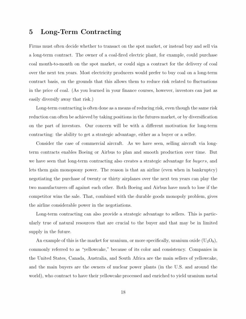
Figure 5: Uranium Fuel Cycle

that is about 50% U235 for use in fuel rods. (Figure 5 shows the uranium fuel cycle.)

Beginning in 1973, an international uranium cartel formed, and pushed the price of

yellowcake from about $5.00 per pound to about $45.00 per pound over a period of two or

three years. Long-term contracting facilitated their ability to push prices up sharply. Electric

utilities had spent billions of dollars on nuclear power plants, and those plants would not run

without uranium. Power plant owners wanted to line up supplies of uranium over fifteen or

twenty years, and as prices rose, they became frantic over the availability of future supplies.

As a result, uranium producers were able to lock in high prices over periods of fifteen or

more years, even though (after the cartel was discovered), the spot price fell back to about

$10.00 per pound.

The uranium cartel is a somewhat extreme example. It is ofen the case, however, that a

natural resource is a critical input for an industrial producer. Electrical equipment manu-

facturers, for example, cannot operate without a steady supply of copper. That dependence

enables copper refiners to sell under long-term contracts at prices well above average spot

prices.

19