Embed Size (px)
Citation preview
LECTURE NOTES ON FINITE ELEMENT ANALYSIS
Prof. Niels Højen Østergaard, University of Applied Sciences Hochschule Rhein-Waal
April 6, 2015
1 Introduction
These lecture notes were written as teaching material for courses in finite element analysisat the University of Applied Sciences Rhein-Waal (Hochschule Rhein-Waal). The notesmay both be applied as stand-alone teaching material for courses introducing finiteelement techniques to students who do not have mechanical engineering as main subject,and as supplementary to text books for students in mechanical engineering.In the lecture notes, the basic mechanical concepts of bars and plane stress elementsare summarized, before the differential equations governing the considered problems areconverted to finite element formulations.Students who are familiar with the general theory of elasticity are encouraged anywayto read the summaries contained in these notes, since it is crusial to have the details ofthe basic theories in mind when studying the details of finite element methods.The present section contains a brief introduction to the method and the underlyingprinciples.The code examples contained in these notes were written using the GNU Octave 3.0.0-beta version. They should work in MATLAB as well, but minor modifications may berequired.Bugs and typos can be reported to [email protected].
1.1 What is finite element analysis (FEA)
The finite element method (FEM) is a method for approximating solutions to differentialequations. In mechanical, civil and structural engineering, finite element analysis (FEA)is applied for design of virtually all systems and components, which are too complexto analyze using analytical methods and hand calculatons. Typical results obtained byFEA are stresses and strains, forces and deformations.Industrial application of FEM for design purposes originates from analysis of aeroplanewings during World War II. Further developments of the method were conducted in theaerospace industry in the late 40s and early 50s, leading to the formulation techniques,which today are implemented in a high number of commercially available computer pro-gramms. Examples of such are Ansys, Abaqus, Nastran (developed by NASA), Cosmos(for SolidWorks), and Mechanica (for Pro/Engineer). The method is widely applied for
1
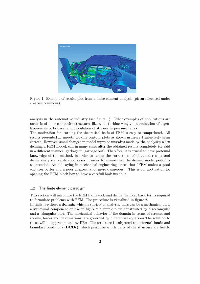
Figure 1: Example of results plot from a finite element analysis (picture licensed undercreative commons)
analysis in the automotive industry (see figure 1). Other examples of applications areanalysis of fiber composite structures like wind turbine wings, determination of eigen-frequencies of bridges, and calculation of stresses in pressure tanks.The motivation for learning the theoretical basis of FEM is easy to comprehend. Allresults presented in smooth looking contour plots as shown in figure 1 intuitively seemcorrect. However, small changes in model input or mistakes made by the analysist whendefining a FEM-model, can in many cases alter the obtained results completely (or saidin a different manner: garbage in, garbage out). Therefore, it is crusial to have profoundknowledge of the method, in order to assess the correctness of obtained results anddefine analytical verification cases in order to ensure that the defined model performsas intended. An old saying in mechanical engineering states that ”FEM makes a goodengineer better and a poor engineer a lot more dangerous”. This is our motivation foropening the FEM-black box to have a carefull look inside it.
1.2 The finite element paradigm
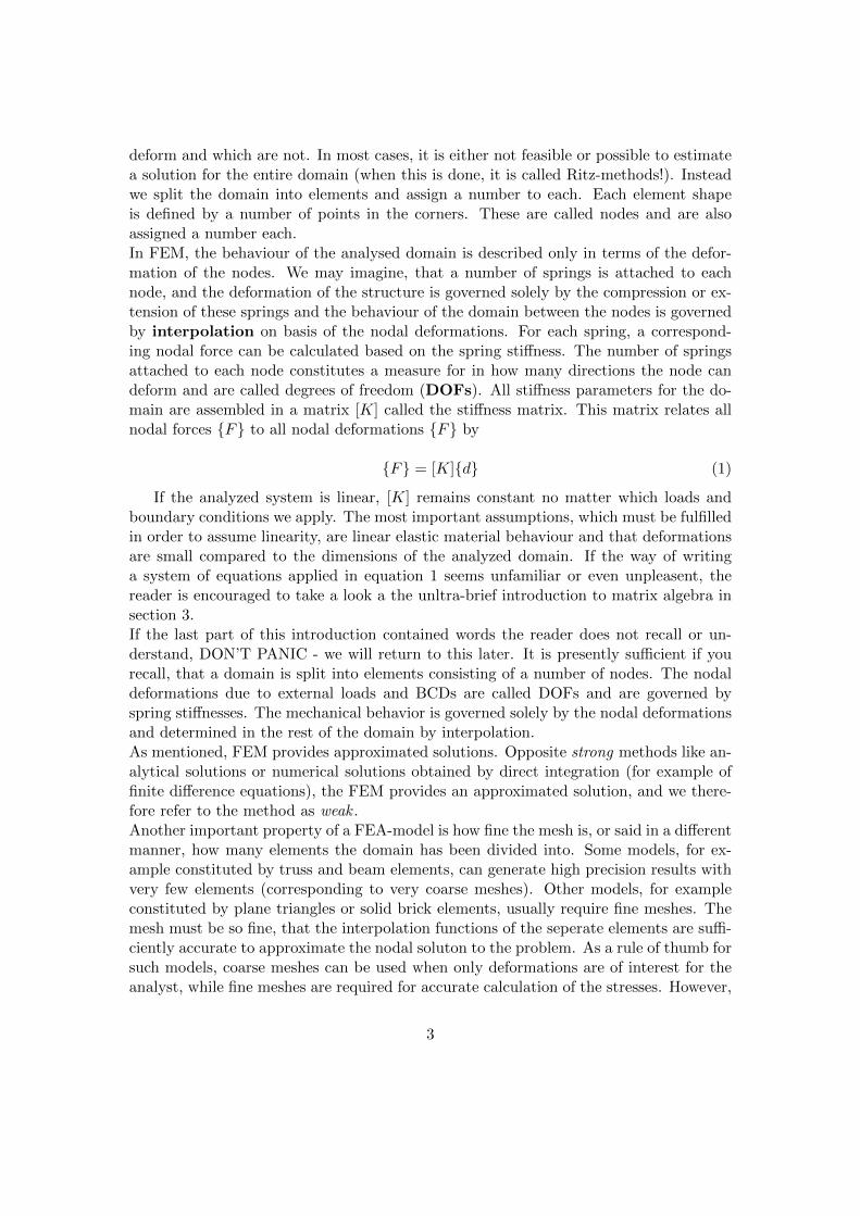
This section will introduce the FEM framework and define the most basic terms requiredto formulate problems with FEM. The procedure is visualized in figure 2.Initially, we chose a domain which is subject of analysis. This can be a mechanical part,a structural component or like in figure 2 a simple plate constituted by a rectangularand a triangular part. The mechanical behavior of the domain in terms of stresses andstrains, forces and deformations, are governed by differential equations.The solution tothose will be approximated by FEA. The structure is subjected to external loads andboundary conditions (BCDs), which prescribe which parts of the structure are free to
2
deform and which are not. In most cases, it is either not feasible or possible to estimatea solution for the entire domain (when this is done, it is called Ritz-methods!). Insteadwe split the domain into elements and assign a number to each. Each element shapeis defined by a number of points in the corners. These are called nodes and are alsoassigned a number each.In FEM, the behaviour of the analysed domain is described only in terms of the defor-mation of the nodes. We may imagine, that a number of springs is attached to eachnode, and the deformation of the structure is governed solely by the compression or ex-tension of these springs and the behaviour of the domain between the nodes is governedby interpolation on basis of the nodal deformations. For each spring, a correspond-ing nodal force can be calculated based on the spring stiffness. The number of springsattached to each node constitutes a measure for in how many directions the node candeform and are called degrees of freedom (DOFs). All stiffness parameters for the do-main are assembled in a matrix [K] called the stiffness matrix. This matrix relates allnodal forces {F} to all nodal deformations {F} by
{F} = [K]{d} (1)
If the analyzed system is linear, [K] remains constant no matter which loads andboundary conditions we apply. The most important assumptions, which must be fulfilledin order to assume linearity, are linear elastic material behaviour and that deformationsare small compared to the dimensions of the analyzed domain. If the way of writinga system of equations applied in equation 1 seems unfamiliar or even unpleasent, thereader is encouraged to take a look a the unltra-brief introduction to matrix algebra insection 3.If the last part of this introduction contained words the reader does not recall or un-derstand, DON’T PANIC - we will return to this later. It is presently sufficient if yourecall, that a domain is split into elements consisting of a number of nodes. The nodaldeformations due to external loads and BCDs are called DOFs and are governed byspring stiffnesses. The mechanical behavior is governed solely by the nodal deformationsand determined in the rest of the domain by interpolation.As mentioned, FEM provides approximated solutions. Opposite strong methods like an-alytical solutions or numerical solutions obtained by direct integration (for example offinite difference equations), the FEM provides an approximated solution, and we there-fore refer to the method as weak .Another important property of a FEA-model is how fine the mesh is, or said in a differentmanner, how many elements the domain has been divided into. Some models, for ex-ample constituted by truss and beam elements, can generate high precision results withvery few elements (corresponding to very coarse meshes). Other models, for exampleconstituted by plane triangles or solid brick elements, usually require fine meshes. Themesh must be so fine, that the interpolation functions of the seperate elements are suffi-ciently accurate to approximate the nodal soluton to the problem. As a rule of thumb forsuch models, coarse meshes can be used when only deformations are of interest for theanalyst, while fine meshes are required for accurate calculation of the stresses. However,
3
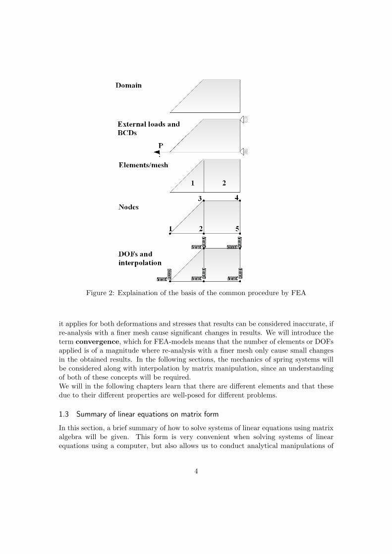
Figure 2: Explaination of the basis of the common procedure by FEA
it applies for both deformations and stresses that results can be considered inaccurate, ifre-analysis with a finer mesh cause significant changes in results. We will introduce theterm convergence, which for FEA-models means that the number of elements or DOFsapplied is of a magnitude where re-analysis with a finer mesh only cause small changesin the obtained results. In the following sections, the mechanics of spring systems willbe considered along with interpolation by matrix manipulation, since an understandingof both of these concepts will be required.We will in the following chapters learn that there are different elements and that thesedue to their different properties are well-posed for different problems.
1.3 Summary of linear equations on matrix form
In this section, a brief summary of how to solve systems of linear equations using matrixalgebra will be given. This form is very convenient when solving systems of linearequations using a computer, but also allows us to conduct analytical manipulations of
4
large systems of equations in an efficient manner. In order to provide a brief and simpleexplenation, the case of a two dimensional linear system will be considered
y = a1x+ b1 (2)
y = a2x+ b2
The solution (x, y) to this system is constituted by the variables which simultanouslyfulfill both of the linear equations. The equations are in plane geometry visualized astwo straight lines with slopes a1 and a2 and intersections with the y-axis b1 and b2where (x, y) are the coordinates of the points where the lines intersect. The two linearequations can be rewritten on the form
b1 = −a1x+ y (3)
b2 = −a2x+ y
On matrix form, equation 3 can be written as follows{b1b2
}=
[−a1 1−a2 1
]{xy
}=
{−a1x+ y−a2x+ y
}(4)
It is noted that a matrix is multiplied with a column vector by the technique demon-strated in the equation. Hence, the product is a vector. Utilizing a more compactnotation, the system of equations can be written on the form
{b} = [A]{x} (5)
In order to obtain the solution to the system of equations, x and y must be isolated. Inorder to do so, the matrix [A] must be eliminated from the right side of the equation.This can be done by multiplication of the so-called inverse of the matrix [A], which isdenoted [A]−1. Always remembering that matrix multiplication is a non-commulativemathmatical operation (hence, multiplication from left and right produce different re-sults), the following expression is obtained
[A]−1{b} = [A]−1[A]{x} = {x} (6)
in which we have utilized that [A]−1[A] = [I]. [I] is the identity matrix which for the2D case is given by
[I] =
[1 00 1
](7)
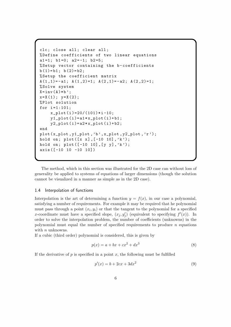
It is observed that multiplication of a matrix with its own inverse cancels out the matrix.A matrix with no inverse is called singular.In the following, the procedure outlined above is demonstrated as a calculated example.The system shown below will have (x, y) = (2.5, 2.5) as solution, which in figure 3is visualized as the intersection between the two lines (drawn in red and blue). Theintersection is marked with black lines.
5
clc; close all; clear all;
%Define coefficients of two linear equations
a1=1; b1=0; a2=-1; b2=5;
%Setup vector containing the b-coefficients
b(1)=b1; b(2)=b2;
%Setup the coefficient matrix
A(1,1)=-a1; A(1 ,2)=1; A(2,1)=-a2; A(2 ,2)=1;
%Solve system
X=inv(A)*b’;
x=X(1); y=X(2);
%Plot solution
for i=1:101;
x_plot(i)=20/(101)*i-10;
y1_plot(i)=a1*x_plot(i)+b1;
y2_plot(i)=a2*x_plot(i)+b2;
end
plot(x_plot ,y1_plot ,’b’,x_plot ,y2_plot ,’r’);
hold on; plot([x x],[-10 10],’k’);
hold on; plot ([-10 10],[y y],’k’);
axis ([-10 10 -10 10])
The method, which in this section was illustrated for the 2D case can without loss ofgenerality be applied to systems of equations of larger dimensions (though the solutioncannot be visualized in a manner as simple as in the 2D case).
1.4 Interpolation of functions
Interpolation is the art of determining a function y = f(x), in our case a polynomial,satisfying a number of requirements. For example it may be required that he polynomialmust pass through a point (xi, yi) or that the tangent to the polynomial for a specifiedx-coordinate must have a specified slope, (xj , y
′j) (equivalent to specifying f ′(x)). In
order to solve the interpolation problem, the number of coefficients (unknowns) in thepolynomial must equal the number of specified requirements to produce n equationswith n unknowns.If a cubic (third order) polynomial is considered, this is given by
p(x) = a+ bx+ cx2 + dx3 (8)
If the derivative of p is specified in a point x, the following must be fulfilled
p′(x) = b+ 2cx+ 3dx2 (9)
6
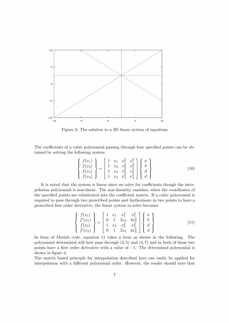
Figure 3: The solution to a 2D linear system of equations
The coefficients of a cubic polynomial passing through four specified points can be ob-tained by solving the following system
f(x1)f(x2)f(x3)f(x4)
=
1 x1 x2
1 x31
1 x2 x22 x3
2
1 x3 x23 x3
3
1 x4 x24 x3
4
abdd
(10)
It is noted that the system is linear since we solve for coefficients though the inter-polation polynomial is non-linear. The non-linearity vanishes, when the coordinates ofthe specified points are substituted into the coefficient matrix. If a cubic polynomial isrequired to pass through two prescribed points and furthermore in two points to have aprescribed first order derivative, the linear system to solve becomes
f(x1)f ′(x1)f(x2)f ′(x2)
=
1 x1 x2
1 x31
0 1 2x2 3x22
1 x3 x23 x3
3
0 1 2x4 3x24
abdd
(11)
In form of Matlab code, equation 11 takes a form as shown in the following. Thepolynomial determined will here pass through (2, 5) and (4, 7) and in both of these twopoints have a first order derivative with a value of −1. The determined polynomial isshown in figure 4.The matrix based principle for interpolation described here can easily be applied forinterpolation with a different polynomial order. However, the reader should note that
7
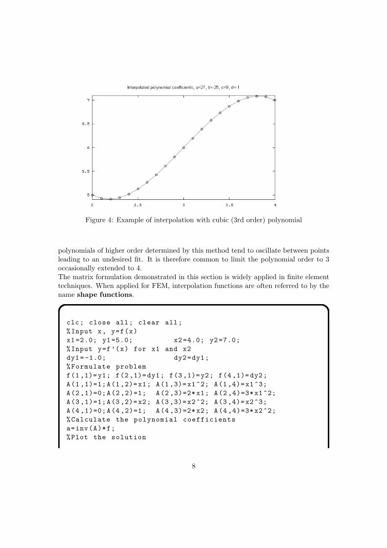
Figure 4: Example of interpolation with cubic (3rd order) polynomial
polynomials of higher order determined by this method tend to oscillate between pointsleading to an undesired fit. It is therefore common to limit the polynomial order to 3occasionally extended to 4.The matrix formulation demonstrated in this section is widely applied in finite elementtechniques. When applied for FEM, interpolation functions are often referred to by thename shape functions.
clc; close all; clear all;
%Input x, y=f(x)
x1=2.0; y1=5.0; x2=4.0; y2 =7.0;
%Input y=f’(x) for x1 and x2
dy1= -1.0; dy2=dy1;
%Formulate problem
f(1,1)=y1; f(2,1)=dy1; f(3 ,1)=y2; f(4 ,1)=dy2;
A(1 ,1)=1;A(1,2)=x1; A(1 ,3)=x1^2; A(1 ,4)=x1^3;
A(2 ,1)=0;A(2 ,2)=1; A(2 ,3)=2*x1; A(2 ,4)=3*x1^2;
A(3 ,1)=1;A(3,2)=x2; A(3 ,3)=x2^2; A(3 ,4)=x2^3;
A(4 ,1)=0;A(4 ,2)=1; A(4 ,3)=2*x2; A(4 ,4)=3*x2^2;
%Calculate the polynomial coefficients
a=inv(A)*f;
%Plot the solution
8
for i=1:21;
x(i)=(x2 -x1 )/20*(i-1)+x1;
y(i)=[1 x(i) x(i)^2 x(i)^3]*a;
end
figure;plot(x,y,’ko -’)
1.5 A single linear elastic spring
In the present section, the stiffness matrix of a single linear elastic spring is derived. Bylinear elastic, it is meant that the relation between force and deformation is linear, seefigure 5.Initially, the right end of the spring will be fixed by setting u2 = 0. This yields thefollowing equation ∑
Fx,1 = ku1 (12)
From equilibrium (ΣFx = 0) it follows that∑Fx,2 = −ku1 = −Fx,1 (13)
Now instead fixing the left end by setting u1 = 0, the following equation must hold∑Fx,2 = −Fx,2 = −ku1 (14)
Superposition of these two equations provides the expressions
Fx,1 = ku1 + ku2 (15)
Fx,2 = −ku2 + ku1 (16)
These two equations with two unknowns can easily be converted to matrix form{Fx,1Fx,2
}=
[k −k−k k
]{u1
u2
}(17)
On compact form, this is written
{F} = [K]{d} (18)
1.6 Two linear elastic springs in line
We shall now consider the problem of assembling a stiffness matrix for more than oneelement. Two springs connected in series will be considered, see figure 6. Initially, onlydeformation of the first node will be considered. Hence, u2 = u3 = 0. The first nodalforce can be determined by
Fx,1 = kau1 = −Fx,2 (19)
9
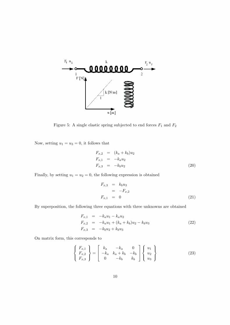
Figure 5: A single elastic spring subjected to end forces F1 and F2
Now, setting u1 = u3 = 0, it follows that
Fx,2 = (ka + kb)u2
Fx,1 = −kau2
Fx,3 = −kbu2 (20)
Finally, by setting u1 = u2 = 0, the following expression is obtained
Fx,3 = kbu3
= −Fx,2Fx,1 = 0 (21)
By superposition, the following three equations with three unknowns are obtained
Fx,1 = −kau1 − kau2
Fx,2 = −kau1 + (ka + kb)u2 − kbu3 (22)
Fx,3 = −kbu2 + kbu3
On matrix form, this corresponds toFx,1Fx,2Fx,3
=
ka −ka 0−ka ka + kb −kb
0 −kb kb
u1
u2
u3
(23)
10
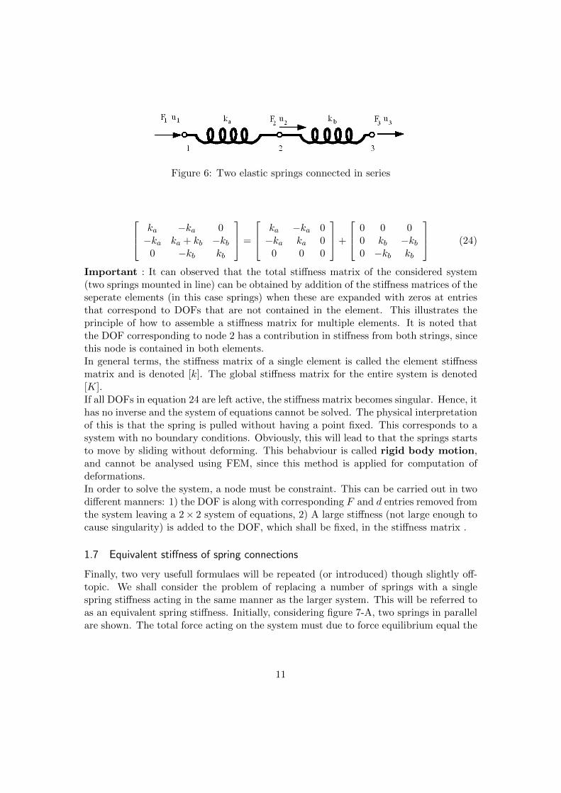
Figure 6: Two elastic springs connected in series
ka −ka 0−ka ka + kb −kb
0 −kb kb
=
ka −ka 0−ka ka 0
0 0 0
+
0 0 00 kb −kb0 −kb kb
(24)
Important : It can observed that the total stiffness matrix of the considered system(two springs mounted in line) can be obtained by addition of the stiffness matrices of theseperate elements (in this case springs) when these are expanded with zeros at entriesthat correspond to DOFs that are not contained in the element. This illustrates theprinciple of how to assemble a stiffness matrix for multiple elements. It is noted thatthe DOF corresponding to node 2 has a contribution in stiffness from both strings, sincethis node is contained in both elements.In general terms, the stiffness matrix of a single element is called the element stiffnessmatrix and is denoted [k]. The global stiffness matrix for the entire system is denoted[K].If all DOFs in equation 24 are left active, the stiffness matrix becomes singular. Hence, ithas no inverse and the system of equations cannot be solved. The physical interpretationof this is that the spring is pulled without having a point fixed. This corresponds to asystem with no boundary conditions. Obviously, this will lead to that the springs startsto move by sliding without deforming. This behabviour is called rigid body motion,and cannot be analysed using FEM, since this method is applied for computation ofdeformations.In order to solve the system, a node must be constraint. This can be carried out in twodifferent manners: 1) the DOF is along with corresponding F and d entries removed fromthe system leaving a 2× 2 system of equations, 2) A large stiffness (not large enough tocause singularity) is added to the DOF, which shall be fixed, in the stiffness matrix .
1.7 Equivalent stiffness of spring connections
Finally, two very usefull formulaes will be repeated (or introduced) though slightly off-topic. We shall consider the problem of replacing a number of springs with a singlespring stiffness acting in the same manner as the larger system. This will be referred toas an equivalent spring stiffness. Initially, considering figure 7-A, two springs in parallelare shown. The total force acting on the system must due to force equilibrium equal the
11
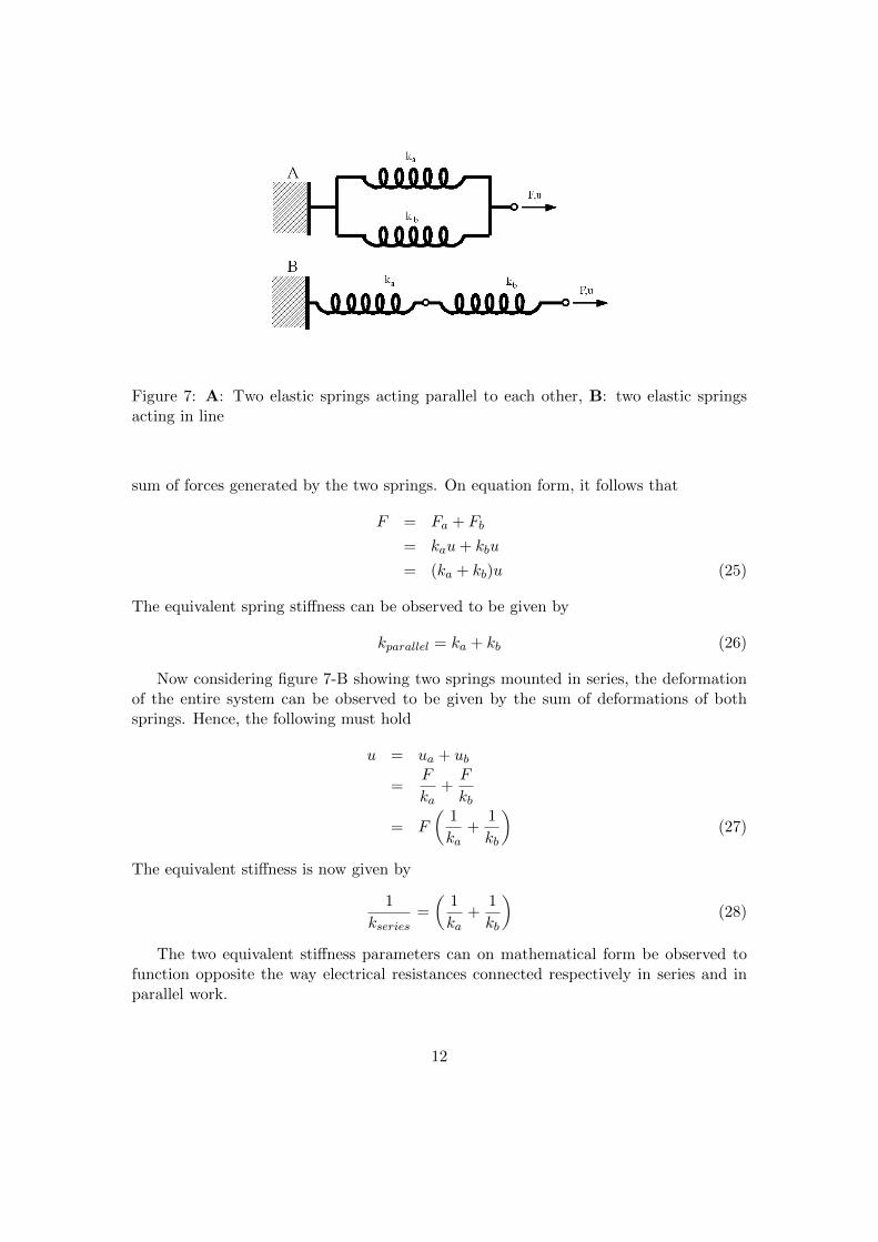
Figure 7: A: Two elastic springs acting parallel to each other, B: two elastic springsacting in line
sum of forces generated by the two springs. On equation form, it follows that
F = Fa + Fb
= kau+ kbu
= (ka + kb)u (25)
The equivalent spring stiffness can be observed to be given by
kparallel = ka + kb (26)
Now considering figure 7-B showing two springs mounted in series, the deformationof the entire system can be observed to be given by the sum of deformations of bothsprings. Hence, the following must hold
u = ua + ub
=F
ka+F
kb
= F
(1
ka+
1
kb
)(27)
The equivalent stiffness is now given by
1
kseries=
(1
ka+
1
kb
)(28)
The two equivalent stiffness parameters can on mathematical form be observed tofunction opposite the way electrical resistances connected respectively in series and inparallel work.
12
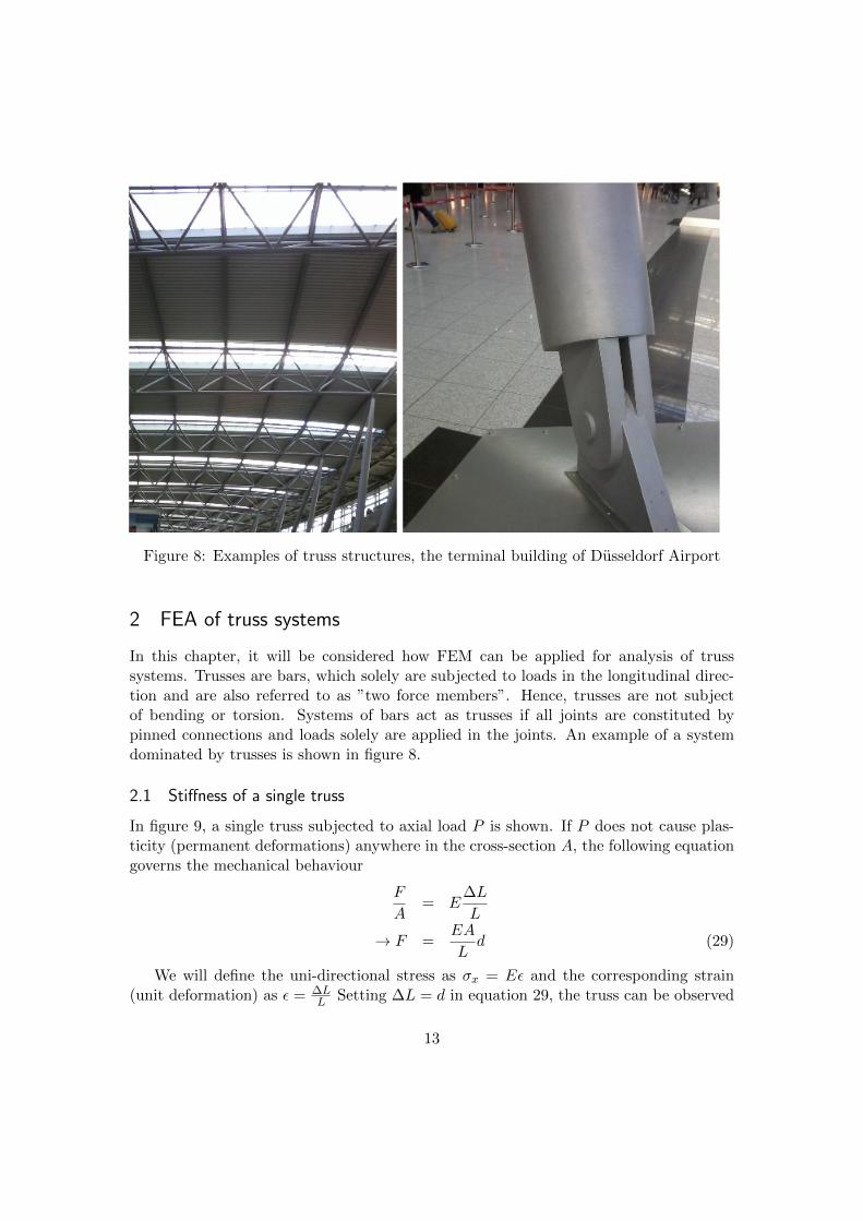
Figure 8: Examples of truss structures, the terminal building of Dusseldorf Airport
2 FEA of truss systems
In this chapter, it will be considered how FEM can be applied for analysis of trusssystems. Trusses are bars, which solely are subjected to loads in the longitudinal direc-tion and are also referred to as ”two force members”. Hence, trusses are not subjectof bending or torsion. Systems of bars act as trusses if all joints are constituted bypinned connections and loads solely are applied in the joints. An example of a systemdominated by trusses is shown in figure 8.
2.1 Stiffness of a single truss
In figure 9, a single truss subjected to axial load P is shown. If P does not cause plas-ticity (permanent deformations) anywhere in the cross-section A, the following equationgoverns the mechanical behaviour
F
A= E
∆L
L
→ F =EA
Ld (29)
We will define the uni-directional stress as σx = Eε and the corresponding strain(unit deformation) as ε = ∆L
L Setting ∆L = d in equation 29, the truss can be observed
13
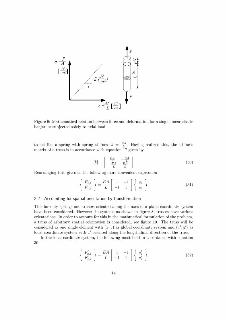
Figure 9: Mathematical relation between force and deformation for a single linear elasticbar/truss subjected solely to axial load
to act like a spring with spring stiffness k = EAL . Having realized this, the stiffness
matrix of a truss is in accordance with equation 17 given by
[k] =
[EAL −EA
L
−EAL
EAL
](30)
Rearranging this, gives us the following more convenient expression{Fx,1Fx,2
}=EA
L
[1 −1−1 1
]{u1
u2
}(31)
2.2 Accounting for spatial orientation by transformation
This far only springs and trusses oriented along the axes of a plane coordinate systemhave been considered. However, in systems as shown in figure 8, trusses have variousorientations. In order to account for this in the mathmatical formulation of the problem,a truss of arbitrary spatial orientation is considered, see figure 10. The truss will beconsidered as one single element with (x, y) as global coordinate system and (x′, y′) aslocal coordinate system with x′ oriented along the longitudinal direction of the truss.
In the local cordinate system, the following must hold in accordance with equation30 {
F ′x,1F ′x,2
}=EA
L
[1 −1−1 1
]{u′1u′2
}(32)
14
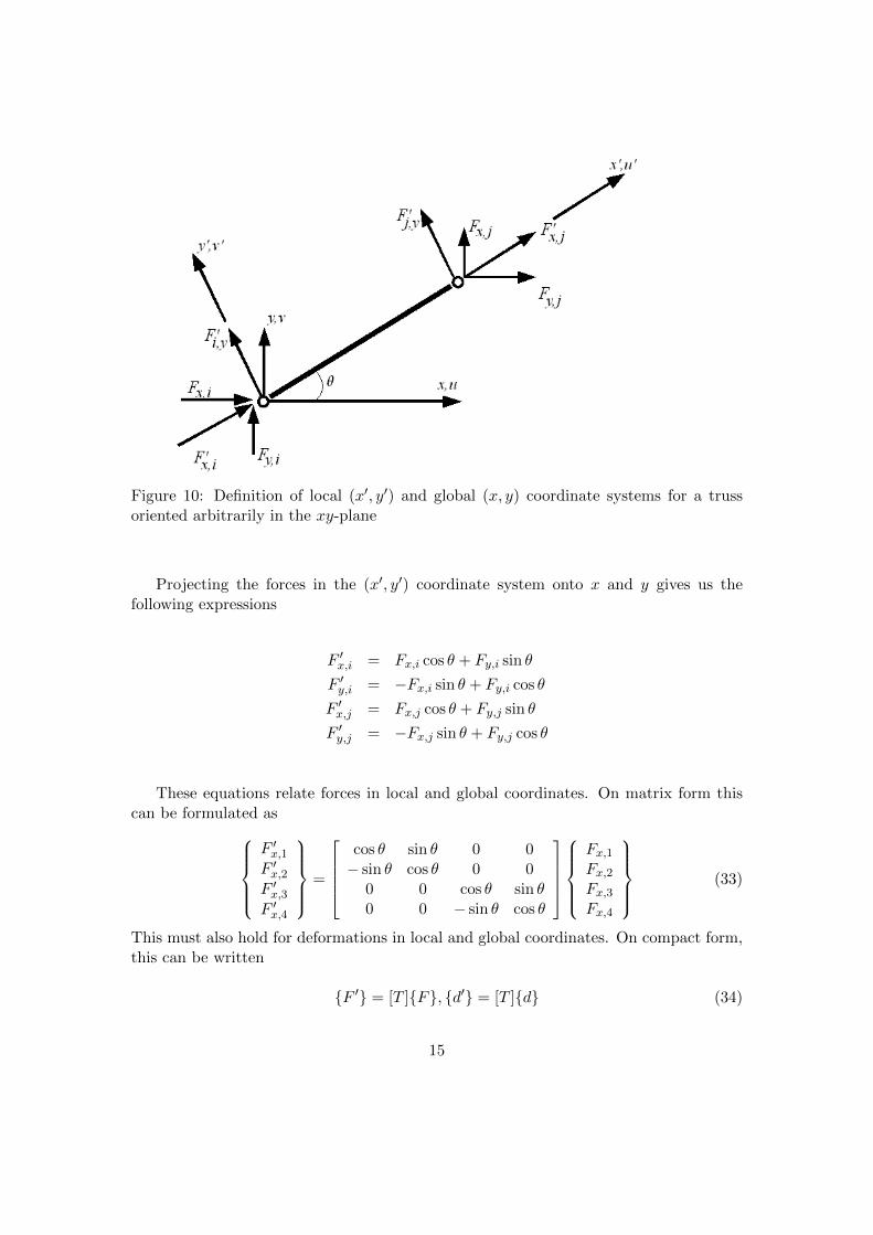
Figure 10: Definition of local (x′, y′) and global (x, y) coordinate systems for a trussoriented arbitrarily in the xy-plane
Projecting the forces in the (x′, y′) coordinate system onto x and y gives us thefollowing expressions
F ′x,i = Fx,i cos θ + Fy,i sin θ
F ′y,i = −Fx,i sin θ + Fy,i cos θ
F ′x,j = Fx,j cos θ + Fy,j sin θ
F ′y,j = −Fx,j sin θ + Fy,j cos θ
These equations relate forces in local and global coordinates. On matrix form thiscan be formulated as
F ′x,1F ′x,2F ′x,3F ′x,4
=
cos θ sin θ 0 0− sin θ cos θ 0 0
0 0 cos θ sin θ0 0 − sin θ cos θ
Fx,1Fx,2Fx,3Fx,4
(33)
This must also hold for deformations in local and global coordinates. On compact form,this can be written
{F ′} = [T ]{F}, {d′} = [T ]{d} (34)
15
The governing equations on matrix form are in local coordinates in accordance withequation 30 given by
{F ′} = [k′]{d′} (35)
Substituting the transformation given in equation 34 into this gives
{T}{F} = [k′]{T}{d} (36)
The governing equation in global coordinates is now
{F} = {T}−1[k′]{T}{d}= {T}T [k′]{T}{d} (37)
since [T ]−1 = [T ]T due to the orthogonality property of the transformation matrix.The global stiffness matrix is therefore given by
[k] = [T ]T [k′]{T} (38)
Evaluating this equation analytically gives the following results
[k] =EA
L
cos2 θ cos θ sin θ − cos2 θ − cos θ sin θ
cos θ sin θ sin2 θ − cos θ sin θ − sin2 θ− cos2 θ − cos θ sin θ cos2 θ cos θ sin θ− cos θ sin θ − sin2 θ cos θ sin θ sin2 θ
(39)
The stresses can be calculated by
σ =E
L[− cos θ − sinθ cos θsinθ]
uiviujvj
(40)
If the longitudinal forces are required, these can easily be determined from F = σA. Thedirectional sines and cosines can be calculated on basis of geometrical considerations by
cos θ =xj − xiL
, sin θ =yj − yiL
(41)
The theory derived in this section is in combination with the basic knowledge of FEM wegained in chapter 1 sufficient to write an FEM-code for analysis of plane truss systems.The equations can by the same principles as shown above be generalized to three-dimensional truss systems.
16
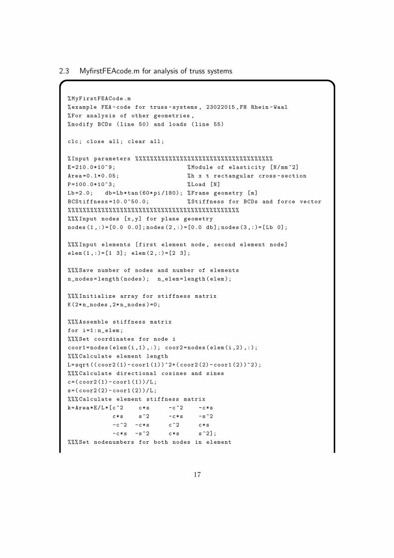
2.3 MyfirstFEAcode.m for analysis of truss systems
%MyFirstFEACode.m
%example FEA -code for truss -systems , 23022015 ,FH Rhein -Waal
%For analysis of other geometries ,
%modify BCDs (line 50) and loads (line 55)
clc; close all; clear all;
%Input parameters %%%%%%%%%%%%%%%%%%%%%%%%%%%%%%%%%%%%%
E=210.0*10^9; %Module of elasticity [N/mm^2]
Area =0.1*0.05; %h x t rectangular cross -section
P=100.0*10^3; %Load [N]
Lb=2.0; db=Lb*tan (60*pi /180); %Frame geometry [m]
BCStiffness =10.0^50.0; %Stiffness for BCDs and force vector
%%%%%%%%%%%%%%%%%%%%%%%%%%%%%%%%%%%%%%%%%%%%%%
%%% Input nodes [x,y] for plane geometry
nodes (1 ,:)=[0.0 0.0]; nodes (2 ,:)=[0.0 db]; nodes (3 ,:)=[Lb 0];
%%% Input elements [first element node , second element node]
elem (1 ,:)=[1 3]; elem (2 ,:)=[2 3];
%%% Save number of nodes and number of elements
n_nodes=length(nodes); n_elem=length(elem);
%%% Initialize array for stiffness matrix
K(2* n_nodes ,2* n_nodes )=0;
%%% Assemble stiffness matrix
for i=1: n_elem;
%%% Set coordinates for node i
coor1=nodes(elem(i,1) ,:); coor2=nodes(elem(i,2) ,:);
%%% Calculate element length
L=sqrt(( coor2(1)- coor1 (1))^2+( coor2(2)- coor1 (2))^2);
%%% Calculate directional cosines and sines
c=( coor2(1)- coor1 (1))/L;
s=( coor2(2)- coor1 (2))/L;
%%% Calculate element stiffness matrix
k=Area*E/L*[c^2 c*s -c^2 -c*s
c*s s^2 -c*s -s^2
-c^2 -c*s c^2 c*s
-c*s -s^2 c*s s^2];
%%% Set nodenumbers for both nodes in element
17
n1=elem(i,1); n2=elem(i,2);
%%% Add element stiffness matrix to global stiffness matrix
K(n1*2-1:n1*2,n1*2-1:n1*2)=K(n1*2-1:n1*2,n1*2-1:n1*2)+k(1:2 ,1:2);
K(n2*2-1:n2*2,n2*2-1:n2*2)=K(n2*2-1:n2*2,n2*2-1:n2*2)+k(3:4 ,3:4);
K(n1*2-1:n1*2,n2*2-1:n2*2)=K(n1*2-1:n1*2,n2*2-1:n2*2)+k(1:2 ,3:4);
K(n2*2-1:n2*2,n1*2-1:n1*2)=K(n2*2-1:n2*2,n1*2-1:n1*2)+k(3:4 ,1:2);
end
%%% Define boundary conditions
K(1,1)= BCStiffness;
K(2,2)= BCStiffness;
K(3,3)= BCStiffness;
K(4,4)= BCStiffness;
%%% Define load vector
F(2* n_nodes )=0; %Initialize array
F(2* n_nodes)=-P; %Define load
%%% Solve for deformations
d=inv(K)*F’
%%% Calculate reaction forces
Rx1=-d(1,1)* BCStiffness
Ry1=-d(2,1)* BCStiffness
Rx2=-d(3,1)* BCStiffness
Ry2=-d(4,1)* BCStiffness
%%% Caluclate sectional forces and stresses for all elements
for i=1: n_elem;
%Following five lines equivalent to those used for calculation of [K]
coor1=nodes(elem(i,1) ,:); coor2=nodes(elem(i,2) ,:);
L=sqrt(( coor2(1)- coor1 (1))^2+( coor2(2)- coor1 (2))^2);
vec=[ coor2(1)- coor1 (1) coor2(2)- coor1 (2)];
c=( coor2(1)- coor1 (1))/L;
s=( coor2(2)- coor1 (2))/L;
%Set element deformations
d_e=[d(2* elem(i,1) -1) d(2* elem(i,1)) d(2* elem(i,2) -1) d(2* elem(i,2))]’
%Calculate stresses
Sigma(i)=E/L*[-c -s c s]*;
%Calculate sectional forces
Tens(i)=Sigma(i)*Area;
end
18
2.4 Calculated example I: simple truss system
In this example, the simple truss system shown in figure 11 will be analyzed in order todetermine a) the reactions at node 1 and 3, b) the stresses in each truss.
In case the reader somehow has forgotten this, force and moment equilibrium mustapply both at global and component level.∑
Fx = 0∑
Fy = 0∑
Mz = 0 (42)
These equations are a special case of ΣF = ma by which the acceleration a is 0 for astatical case. The applied equation is (obviously) Newton’s second law. It will in thefollowing be shown how this works.Considering figure 11, the vertical dimension is given by db = Lbtan(θ); We will nowaim to determine the reaction forces. Global static equilibrium gives us the followingtwo equations ∑
Fx = Rx,1 +Rx,2 = 0→ Rx,1 = −Rx,2 (43)
∑Fy = −P +Ry,1 +Ry,2 = 0 (44)
Equivalently, moment equilibrium provides the equation∑M2 = PLb −Rx,1db → Rx,1 = P
Lbdb
= 0 (45)
Hence, we have Rx,2 = −P Ld . However, this is insufficient to determine all reactions.
Considering component-wise equilibrium and considering the overbar, the following musthold
∑Fx = Fcos(θ) +Rx,2 = 0→ F =
−Rx,2cos(θ)
= PLbdb
1
cos(θ)(46)
∑Fy = −Fsin(θ) +Ry,2 = 0→ Ry,2 = Fsin(θ) = P
Lbdb
sin(θ)
cos(θ)
= PLbdb
dbcos(Lb)
= P (47)
Additionally, the following holds: Ry,1 = P −Ry,2 = P − P = 0Having determined all reaction forces analytically, the FEA codeMyfirstFEAcode.m
can be applied for analysis of the truss system. For the steel material parameters givenin the example and bars of dimensions h× b = 0.1m× 0.05m, L = 2.0m and θ = 60deg,the following reactions are obtained with the code:Rx,1 = 58kN Rx,2 = −58kNRy,1 = 0kN Ry,2 = 100kNThe same values are obtained if the input given above is substituted into the equationsderived for the equilibrium. The stresses are shown in figure 12,B. These correspond tothe values derived analytically using σ = F
A
19
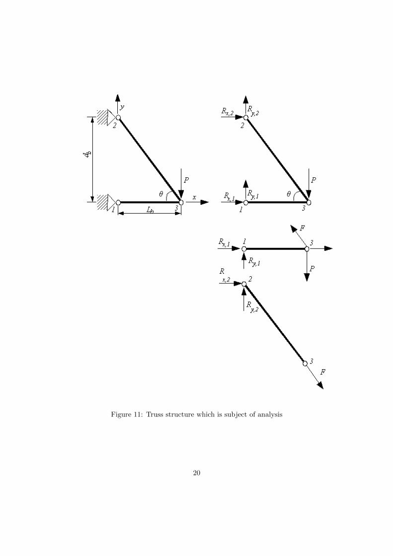
Figure 11: Truss structure which is subject of analysis
20
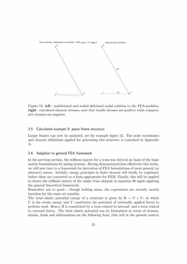
Figure 12: left : undeformed and scaled deformed nodal solution to the FEA-problem,right : calculated element stresses, note that tensile stresses are positive while compres-sive stresses are negative
2.5 Calculated example II: plane frame structure
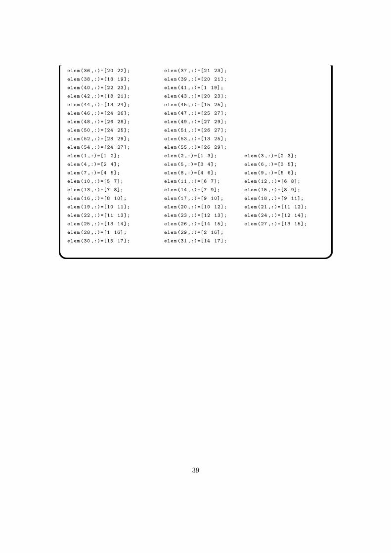
Larger frames can now be analyzed, see for example figure 13. The node coordinatesand element definitions applied for generating this structure is contained in AppendixA.
2.6 Adaption to general FEA framework
In the previous section, the stiffness matrix for a truss was derived on basis of the basicmatrix formulations for spring systems. Having demonstrated how effectively this works,we will now turn to a framework for derivation of FEA formulations of more general (orabstract) nature. Initially, energy principles in finite element will briefly be explained,before these are converted to a form appropriate for FEM. Finally, this will be appliedto derive the stiffness matrix of the single truss element in equation 30 again applyingthe general theoretical framework.Remember not to panic - though looking mean, the expressions are actually mostlyharmless for the cases we consider.The total elastic potential energy of a structure is given by Π = U + V , in whichU is the strain energy and V constitutes the potential of externally applied forces toperform work. Hence, Π is constituted by a term related to internal- and a term relatedto external forces. The total elastic potential can be formulated in terms of stresses,strains, loads and deformations on the following form (this will in the present context
21
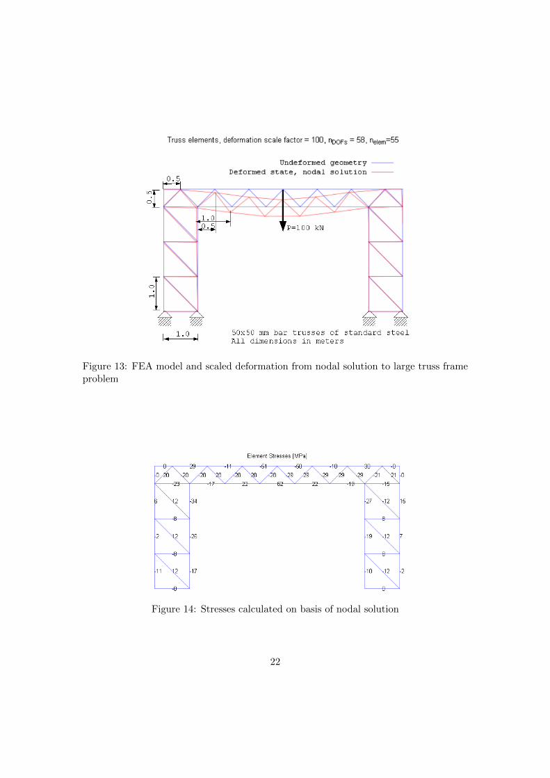
Figure 13: FEA model and scaled deformation from nodal solution to large truss frameproblem
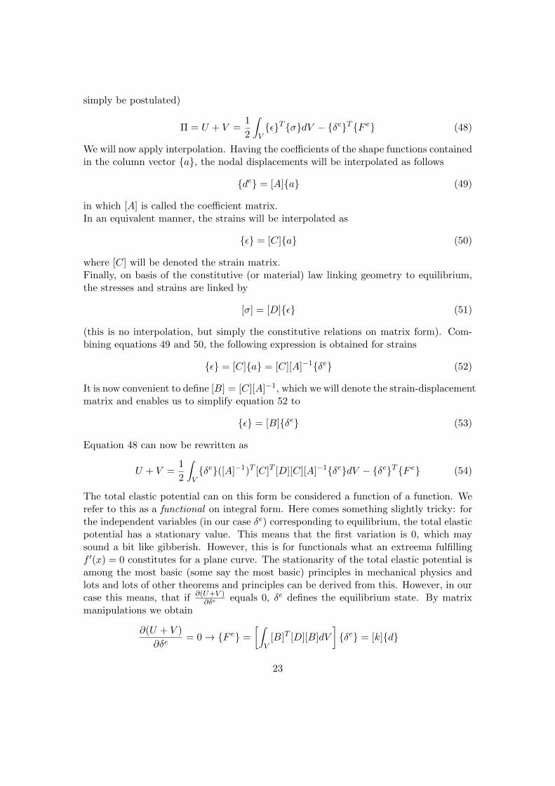
Figure 14: Stresses calculated on basis of nodal solution
22
simply be postulated)
Π = U + V =1
2
∫V{ε}T {σ}dV − {δe}T {F e} (48)
We will now apply interpolation. Having the coefficients of the shape functions containedin the column vector {a}, the nodal displacements will be interpolated as follows
{de} = [A]{a} (49)
in which [A] is called the coefficient matrix.In an equivalent manner, the strains will be interpolated as
{ε} = [C]{a} (50)
where [C] will be denoted the strain matrix.Finally, on basis of the constitutive (or material) law linking geometry to equilibrium,the stresses and strains are linked by
[σ] = [D]{ε} (51)
(this is no interpolation, but simply the constitutive relations on matrix form). Com-bining equations 49 and 50, the following expression is obtained for strains
{ε} = [C]{a} = [C][A]−1{δe} (52)
It is now convenient to define [B] = [C][A]−1, which we will denote the strain-displacementmatrix and enables us to simplify equation 52 to
{ε} = [B]{δe} (53)
Equation 48 can now be rewritten as
U + V =1
2
∫V{δe}([A]−1)T [C]T [D][C][A]−1{δe}dV − {δe}T {F e} (54)
The total elastic potential can on this form be considered a function of a function. Werefer to this as a functional on integral form. Here comes something slightly tricky: forthe independent variables (in our case δe) corresponding to equilibrium, the total elasticpotential has a stationary value. This means that the first variation is 0, which maysound a bit like gibberish. However, this is for functionals what an extreema fulfillingf ′(x) = 0 constitutes for a plane curve. The stationarity of the total elastic potential isamong the most basic (some say the most basic) principles in mechanical physics andlots and lots of other theorems and principles can be derived from this. However, in ourcase this means, that if ∂(U+V )
∂δe equals 0, δe defines the equilibrium state. By matrixmanipulations we obtain
∂(U + V )
∂δe= 0→ {F e} =
[∫V
[B]T [D][B]dV
]{δe} = [k]{d}
23
so let us return to the thruss...The enhanced theoretical framework presented above is not going to ease the derivationin this case. However, a truss element is by nature of such simplicity, that the principleexcellently can be explained for trusses in order for the reader to gain insight in how toapply the framework. For more complex elements, this methodology eases the derivationsa lot.The nodal displacements are given by
{δe} =
{u1
u2
}(55)
(for reference, see figure 10). We will now need to interpolate the displacement fieldbetween u1 and u2. In order to do so, we apply a linear shape function, such that thedeformations u(x) can be determined by
u(x) ≈ f(x) = a+ bx
=[
1 x]{ a
b
}(56)
On compact form, this can be written [f(x)]{a}.Knowing the values of f(x) on the boundaries x = 0 and x = L, the following must hold
u1 = f(0) = a, u2 = f(L) = a+ bL (57)
On matrix form, this can be written{u1
u2
}=
[1 01 L
]{ab
}(58)
On compact form, this can be written {δe}=[A]{a}. Hence, the [A]-matrix has now beenobtained.It is noted that the inverse of [A] is given by
[A]−1 =
[1 0− 1L
1L
](59)
since this will be needed in the following. We will now consider the element strains inorder to derive the [C] matrix. The strain is per definition given by
ε =du
dx≈ df
dx= b (60)
On matrix form, this gives us
ε =[
0 1]{ a
b
}(61)
= [C]{a} (62)
24
Now having determined the [C] matrix, only the relation between stresses and strainsgoverned by [D] is required. This is easily found by considering Hook’s law for uni-directional stress
σ = Eε (63)
It follows that [D] = E. The strain-displacement matrix can now be calculated as
[B] = [C][A]−1
=[
0 1] [ 1 0− 1L
1L
]=
[− 1L
1L
](64)
And that’s it! Everything required to determine the element stiffness matrix hasbeen obtained from the analysis. Plugging [B] and [D] into equation 55, we obtain
[ke] =
∫V
[B]T [D][B]dV
=
∫V
{− 1L
1L
}E[− 1L
1L
]dV
= EAL
[1L2 − 1
L2
− 1L2
1L2
]
=EA
L
[1 −1−1 1
](65)
in which we have taken advantage of that the integral in V simplifies to∫V dV = AL
for bars with constant cross sections, in which A denotes cross-sectional area and Llength. The obtained stiffness matrix can be observed to correspond to the result thatwas derived in equation 30 .
It is common to define the interpolation- or shape function matrix (in this case a rowvector) in the following manner
{N} = [f(x)][A]−1 (66)
This notation is only included in order for the readers to familiarize themselves withit, since it is commonly used in text books and related litterature. In the following, wewill continue to use the notation that was applied in this section. For problems of morecomplex nature it implies multiple advantages, for example that the solutions throughoutthe domain easily can be approximated directly on basis of the nodal solutions and theshape functions organized in a matrix.Summarizing, in order to derive the stiffness matrix, the following matrices are needed:
• The coefficient matrix [A] relating nodal displacements to shape function coeffi-cients
25
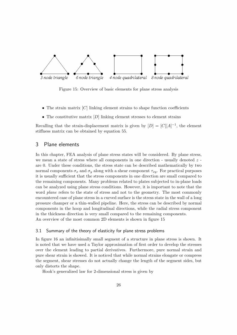
Figure 15: Overview of basic elements for plane stress analysis
• The strain matrix [C] linking element strains to shape function coefficients
• The constitutive matrix [D] linking element stresses to element strains
Recalling that the strain-displacement matrix is given by [D] = [C][A]−1, the elementstiffness matrix can be obtained by equation 55.
3 Plane elements
In this chapter, FEA analysis of plane stress states will be considered. By plane stress,we mean a state of stress where all components in one direction - usually denoted z -are 0. Under these conditions, the stress state can be described mathematically by twonormal components σx and σy along with a shear component τxy. For practical purposesit is usually sufficient that the stress components in one direction are small compared tothe remaining components. Many problems related to plates subjected to in-plane loadscan be analyzed using plane stress conditions. However, it is important to note that theword plane refers to the state of stress and not to the geometry. The most commonlyencountered case of plane stress in a curved surface is the stress state in the wall of a longpressure champer or a thin-walled pipeline. Here, the stress can be described by normalcomponents in the hoop and longitudinal directions, while the radial stress componentin the thickness direction is very small compared to the remaining components.An overview of the most common 2D elements is shown in figure 15
3.1 Summary of the theory of elasticity for plane stress problems
In figure 16 an infinitisimally small segment of a structure in plane stress is shown. Itis noted that we have used a Taylor approximation of first order to develop the stressesover the element leading to partial derivatives. Furthermore, pure normal strain andpure shear strain is showed. It is noticed that while normal strains elongate or compressthe segment, shear stresses do not actually change the length of the segment sides, butonly distorts the shape.
Hook’s generalized law for 2-dimensional stress is given by
26
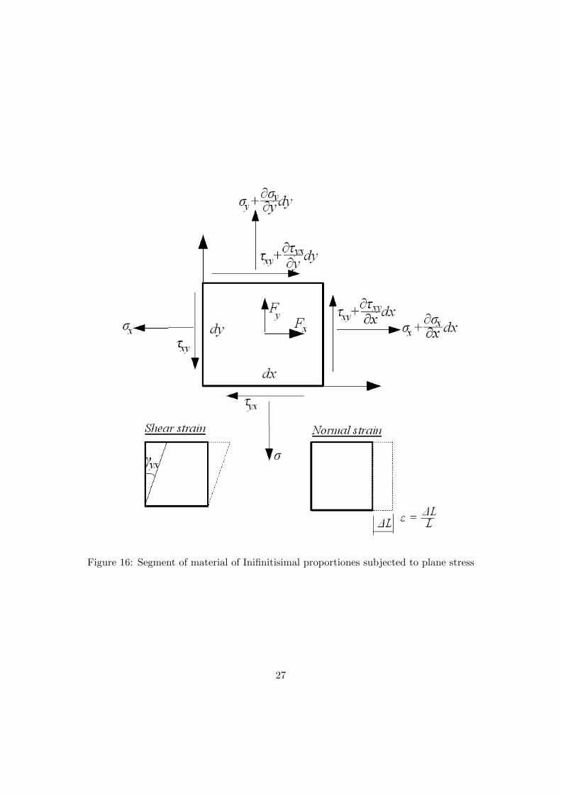
Figure 16: Segment of material of Inifinitisimal proportiones subjected to plane stress
27
εx =σxE− νσy
E(67)
εy =σyE− νσx
E(68)
γxy =τ
G=
2(1 + ν)
Eτxy (69)
These equations are our constitutive relations relating geometry in form of strains (unitdeformations) to equilibrium (stresses). Due to the moment equilibrium it follows thatτxy = τyx.
(σx +
∂σx∂x
dx
)dy − σxdy +
(τxy +
∂τxy∂y
dy
)dx− τxydx+ Fxdxdy = 0
Neglecting higher order terms, this can be reduced to
(∂σx∂x
+∂τxy∂y
+ Fx
)dxdy = 0 (70)
Summing up the forces in the y-direction provides a similar equation governing theforce equilibrium. The equilibrium equations for a state of plane stress are then givenby
∂σx∂x
+∂τxy∂y
+ Fx = 0 (71)
∂σy∂y
+∂τxy∂x
+ Fy = 0 (72)
The forces Fx and Fy are volume forces (also referred to as body forces), which act onthe entire volume considered. Examples of volume forces are gravity and inertia forces.The derivation for a three dimensional general stress state is obtained in an equivalentmanner by force and moment considerations on a unit cube (this will not be repeatedhere). These are given by
∂σx∂x
+∂τxy∂y
+∂τxz∂z
+ Fx = 0 (73)
∂σy∂y
+∂τxy∂x
+∂τyz∂z
+ Fy = 0 (74)
∂σz∂z
+∂τxz∂x
+∂τyz∂y
+ Fz = 0 (75)
Additionally, a set of compability equations, for plane conditions 3, is required toensure that the stresses and strain fields are physically possible. These will not bepresented in this context. Instead, it willl be considered how a triangular element forplane stress analysis can be constructed.
28
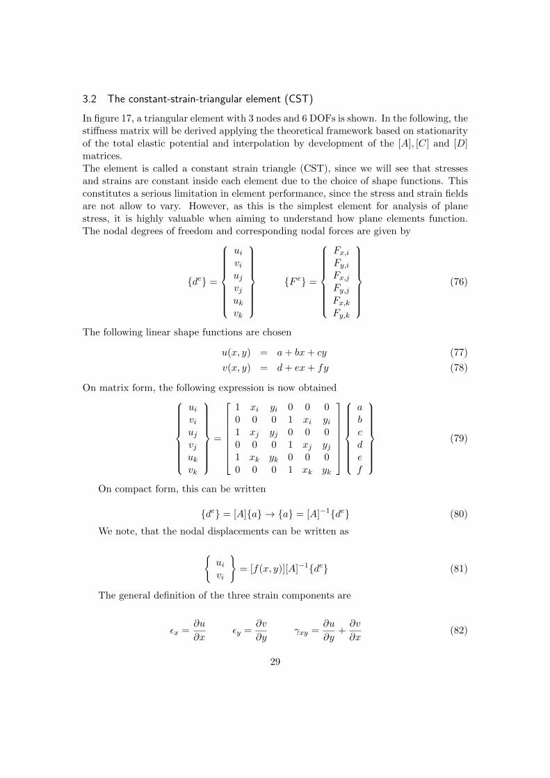
3.2 The constant-strain-triangular element (CST)
In figure 17, a triangular element with 3 nodes and 6 DOFs is shown. In the following, thestiffness matrix will be derived applying the theoretical framework based on stationarityof the total elastic potential and interpolation by development of the [A], [C] and [D]matrices.The element is called a constant strain triangle (CST), since we will see that stressesand strains are constant inside each element due to the choice of shape functions. Thisconstitutes a serious limitation in element performance, since the stress and strain fieldsare not allow to vary. However, as this is the simplest element for analysis of planestress, it is highly valuable when aiming to understand how plane elements function.The nodal degrees of freedom and corresponding nodal forces are given by
{de} =
uiviujvjukvk
{F e} =
Fx,iFy,iFx,jFy,jFx,kFy,k
(76)
The following linear shape functions are chosen
u(x, y) = a+ bx+ cy (77)
v(x, y) = d+ ex+ fy (78)
On matrix form, the following expression is now obtained
uiviujvjukvk
=
1 xi yi 0 0 00 0 0 1 xi yi1 xj yj 0 0 00 0 0 1 xj yj1 xk yk 0 0 00 0 0 1 xk yk
abcdef
(79)
On compact form, this can be written
{de} = [A]{a} → {a} = [A]−1{de} (80)
We note, that the nodal displacements can be written as
{uivi
}= [f(x, y)][A]−1{de} (81)
The general definition of the three strain components are
εx =∂u
∂xεy =
∂v
∂yγxy =
∂u
∂y+∂v
∂x(82)
29
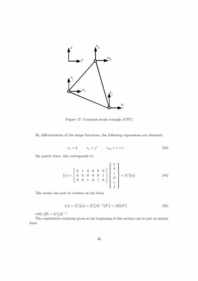
Figure 17: Constant strain triangle (CST)
By differentiation of the shape functions, the following expressions are obtained
εx = b εx = f γxy = c+ e (83)
On matrix form, this corresponds to
{ε} =
0 1 0 0 0 00 0 0 0 0 10 0 1 0 1 0
abcdef
= [C]{a} (84)
The strain can now be written on the form
{ε} = [C]{a} = [C][A]−1{de} = [B]{de} (85)
with [B] = [C][A]−1.The constitutive relations given at the beginning of this section can be put on matrix
form
30
εxεyγxy
=1
E
1 −ν 0−ν 1 00 0 2(1 + ν)
σxσyτxy
(86)
Inverting this matrix equation yields
σxσyτxy
=E
1− ν2
1 ν 0ν 1 0
0 0 (1+ν)2
εxεyγxy
(87)
We recognize the constitutive matrix and can now on compact form write
{σ} = [D]{ε} = [D][B]{de} (88)
The stiffness matrix can now be determined by the general equation that was derivedfrom the principle of stationarity of the total elastic potential
[K] =
∫V
[B]T [D][B]dV = [B]T [D][B]At (89)
The stiffness matrix is not presented in analytical form in this context due to thesize of the array.
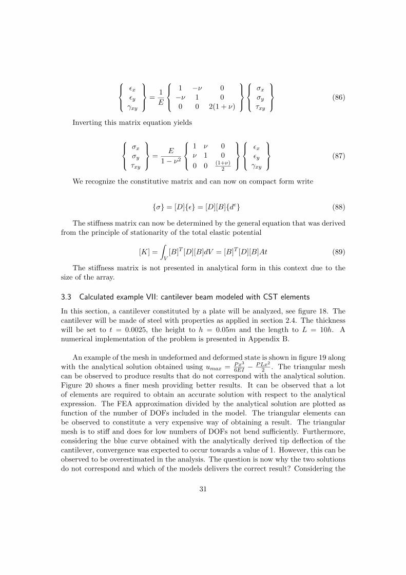
3.3 Calculated example VII: cantilever beam modeled with CST elements
In this section, a cantilever constituted by a plate will be analyzed, see figure 18. Thecantilever will be made of steel with properties as applied in section 2.4. The thicknesswill be set to t = 0.0025, the height to h = 0.05m and the length to L = 10h. Anumerical implementation of the problem is presented in Appendix B.
An example of the mesh in undeformed and deformed state is shown in figure 19 alongwith the analytical solution obtained using umax = Px3
6EI −PLx2
2 . The triangular meshcan be observed to produce results that do not correspond with the analytical solution.Figure 20 shows a finer mesh providing better results. It can be observed that a lotof elements are required to obtain an accurate solution with respect to the analyticalexpression. The FEA approximation divided by the analytical solution are plotted asfunction of the number of DOFs included in the model. The triangular elements canbe observed to constitute a very expensive way of obtaining a result. The triangularmesh is to stiff and does for low numbers of DOFs not bend sufficiently. Furthermore,considering the blue curve obtained with the analytically derived tip deflection of thecantilever, convergence was expected to occur towards a value of 1. However, this can beobserved to be overestimated in the analysis. The question is now why the two solutionsdo not correspond and which of the models delivers the correct result? Considering the
31
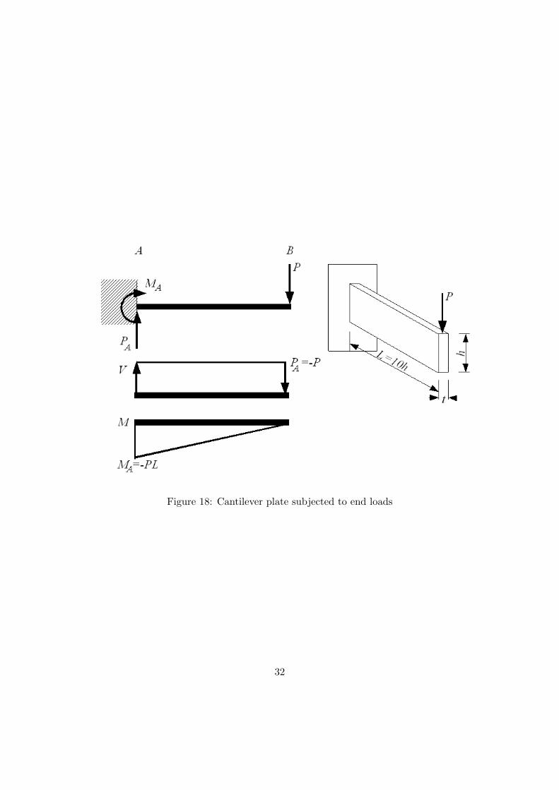
Figure 18: Cantilever plate subjected to end loads
32
Figure 19: Cantilever plate mesh (green) and scaled nodal deformation solution (red)along with analytical solution (blue)
chosen geometry, we note that L/h = 10. This violates the assumption L/h > 12− 15,which serve as basis for the Bernuilli-Euler beam theory. Hence, for the analyzed beamit can no longer be assumed that plane cross-sections remain plane. It follows, that themodel of CLT-elements, though expensive from a computational mechanics perspective,provides a better result than the Bernuilli-Euler expression for cantilever beam.
Beams for which L/h < 12 can be calculated on basis of the Timoshenko-beam the-ory. This theoretical framework accounts for shear contributions to beam deformationsand allow plane cross sections to be distorted due to stress stress. This is illustratedon figure 22 The general theory is complex, but it provides a solution for the specificproblem considered, namely a cantilever beam. This is given by
vy =P
6EI
[3νy2(L− x) + (4 + 5ν)
D2x
4+ (3L− x)x2
](90)
3.4 Closing remarks regarding choice of elements
For analysis of plane stress, 3-node triangles may provide accurate results with low com-putational costs in regions where strain gradients are small. However, in general terms,the element performance is poor and for analysis of critical regions, higher order elementsshould be applied, for example 6-node triangles. The same applies to quadrilateral el-ements. The 3-node triangle and 4-node quadrilateral elements perform poorly due tothe constant stress and strain fields and their lacking ability to represent bending. Thisis illustrated in figure 23.
33
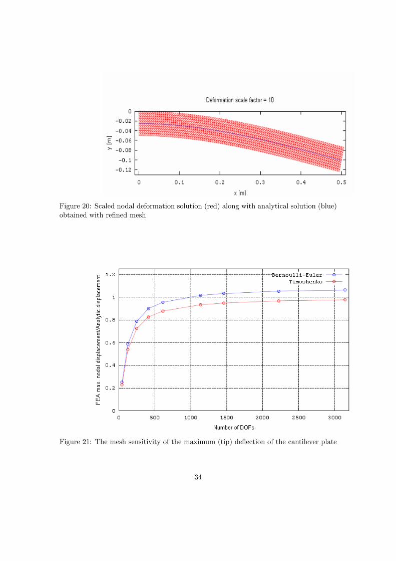
Figure 20: Scaled nodal deformation solution (red) along with analytical solution (blue)obtained with refined mesh
Figure 21: The mesh sensitivity of the maximum (tip) deflection of the cantilever plate
34
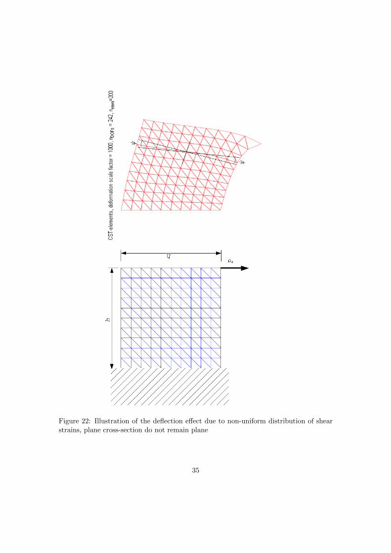
Figure 22: Illustration of the deflection effect due to non-uniform distribution of shearstrains, plane cross-section do not remain plane
35
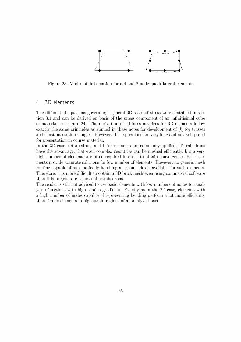
Figure 23: Modes of deformation for a 4 and 8 node quadrilateral elements
4 3D elements
The differential equations governing a general 3D state of stress were contained in sec-tion 3.1 and can be derived on basis of the stress component of an infinitisimal cubeof material, see figure 24. The derivation of stiffness matrices for 3D elements followexactly the same principles as applied in these notes for development of [k] for trussesand constant-strain-triangles. However, the expressions are very long and not well-posedfor presentation in course material.In the 3D case, tetrahedrons and brick elements are commonly applied. Tetrahedronshave the advantage, that even complex geomtries can be meshed efficiently, but a veryhigh number of elements are often required in order to obtain convergence. Brick ele-ments provide accurate solutions for low number of elements. However, no generic meshroutine capable of automatically handling all geometries is available for such elements.Therefore, it is more difficult to obtain a 3D brick mesh even using commercial softwarethan it is to generate a mesh of tetrahedrons.The reader is still not adviced to use basic elements with low numbers of nodes for anal-ysis of sections with high strains gradients. Exactly as in the 2D-case, elements witha high number of nodes capable of representing bending perform a lot more efficientlythan simple elements in high-strain regions of an analyzed part.
36
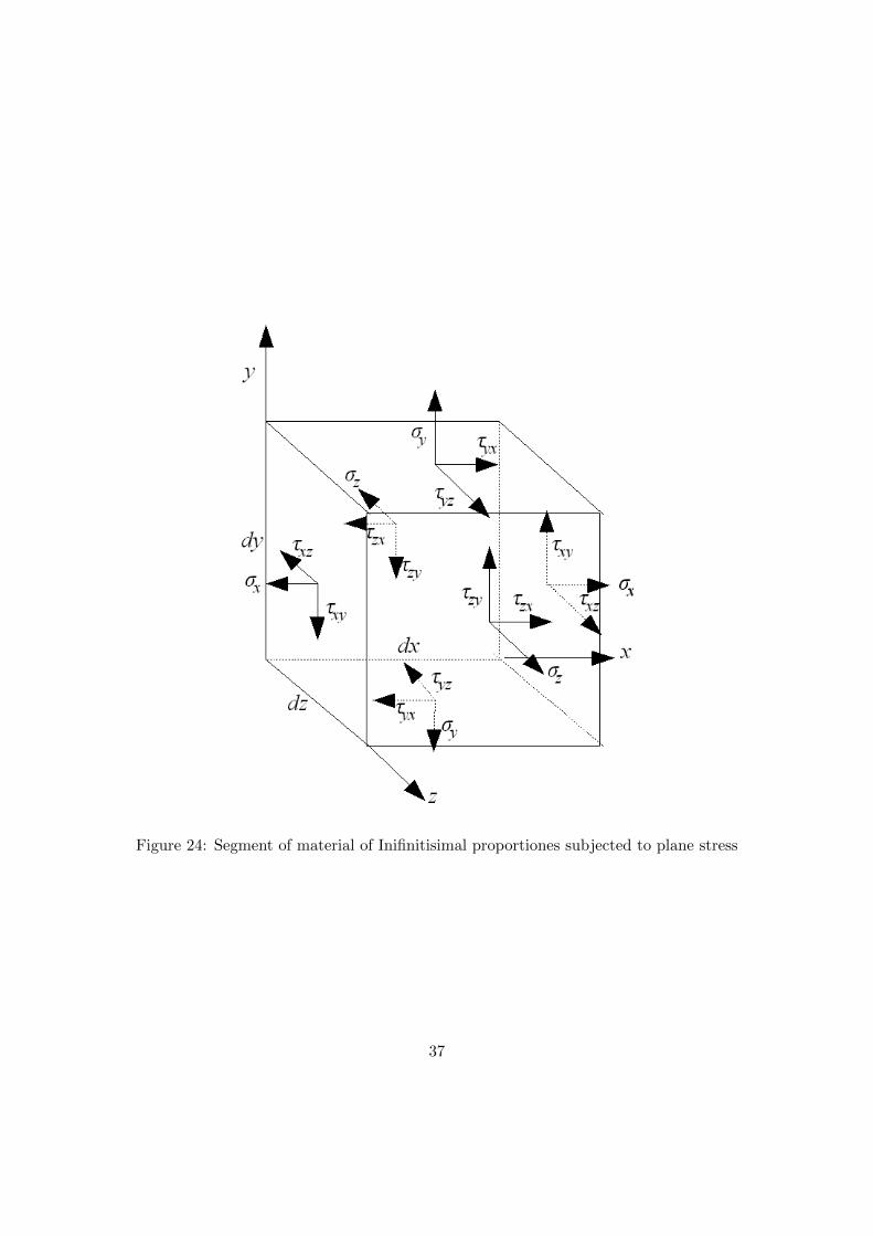
Figure 24: Segment of material of Inifinitisimal proportiones subjected to plane stress
37
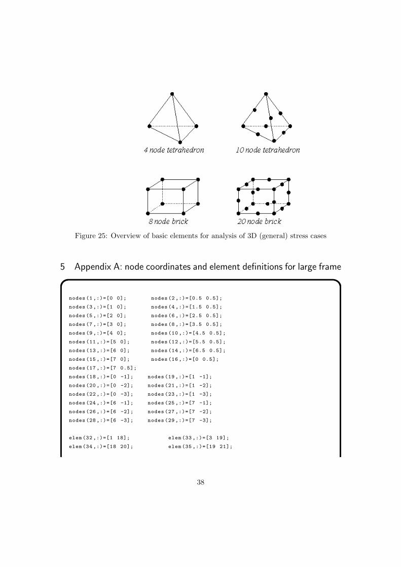
Figure 25: Overview of basic elements for analysis of 3D (general) stress cases
5 Appendix A: node coordinates and element definitions for large frame
nodes (1 ,:)=[0 0]; nodes (2 ,:)=[0.5 0.5];
nodes (3 ,:)=[1 0]; nodes (4 ,:)=[1.5 0.5];
nodes (5 ,:)=[2 0]; nodes (6 ,:)=[2.5 0.5];
nodes (7 ,:)=[3 0]; nodes (8 ,:)=[3.5 0.5];
nodes (9 ,:)=[4 0]; nodes (10 ,:)=[4.5 0.5];
nodes (11 ,:)=[5 0]; nodes (12 ,:)=[5.5 0.5];
nodes (13 ,:)=[6 0]; nodes (14 ,:)=[6.5 0.5];
nodes (15 ,:)=[7 0]; nodes (16 ,:)=[0 0.5];
nodes (17 ,:)=[7 0.5];
nodes (18 ,:)=[0 -1]; nodes (19 ,:)=[1 -1];
nodes (20 ,:)=[0 -2]; nodes (21 ,:)=[1 -2];
nodes (22 ,:)=[0 -3]; nodes (23 ,:)=[1 -3];
nodes (24 ,:)=[6 -1]; nodes (25 ,:)=[7 -1];
nodes (26 ,:)=[6 -2]; nodes (27 ,:)=[7 -2];
nodes (28 ,:)=[6 -3]; nodes (29 ,:)=[7 -3];
elem (32 ,:)=[1 18]; elem (33 ,:)=[3 19];
elem (34 ,:)=[18 20]; elem (35 ,:)=[19 21];
38
elem (36 ,:)=[20 22]; elem (37 ,:)=[21 23];
elem (38 ,:)=[18 19]; elem (39 ,:)=[20 21];
elem (40 ,:)=[22 23]; elem (41 ,:)=[1 19];
elem (42 ,:)=[18 21]; elem (43 ,:)=[20 23];
elem (44 ,:)=[13 24]; elem (45 ,:)=[15 25];
elem (46 ,:)=[24 26]; elem (47 ,:)=[25 27];
elem (48 ,:)=[26 28]; elem (49 ,:)=[27 29];
elem (50 ,:)=[24 25]; elem (51 ,:)=[26 27];
elem (52 ,:)=[28 29]; elem (53 ,:)=[13 25];
elem (54 ,:)=[24 27]; elem (55 ,:)=[26 29];
elem (1 ,:)=[1 2]; elem (2 ,:)=[1 3]; elem (3 ,:)=[2 3];
elem (4 ,:)=[2 4]; elem (5 ,:)=[3 4]; elem (6 ,:)=[3 5];
elem (7 ,:)=[4 5]; elem (8 ,:)=[4 6]; elem (9 ,:)=[5 6];
elem (10 ,:)=[5 7]; elem (11 ,:)=[6 7]; elem (12 ,:)=[6 8];
elem (13 ,:)=[7 8]; elem (14 ,:)=[7 9]; elem (15 ,:)=[8 9];
elem (16 ,:)=[8 10]; elem (17 ,:)=[9 10]; elem (18 ,:)=[9 11];
elem (19 ,:)=[10 11]; elem (20 ,:)=[10 12]; elem (21 ,:)=[11 12];
elem (22 ,:)=[11 13]; elem (23 ,:)=[12 13]; elem (24 ,:)=[12 14];
elem (25 ,:)=[13 14]; elem (26 ,:)=[14 15]; elem (27 ,:)=[13 15];
elem (28 ,:)=[1 16]; elem (29 ,:)=[2 16];
elem (30 ,:)=[15 17]; elem (31 ,:)=[14 17];
39
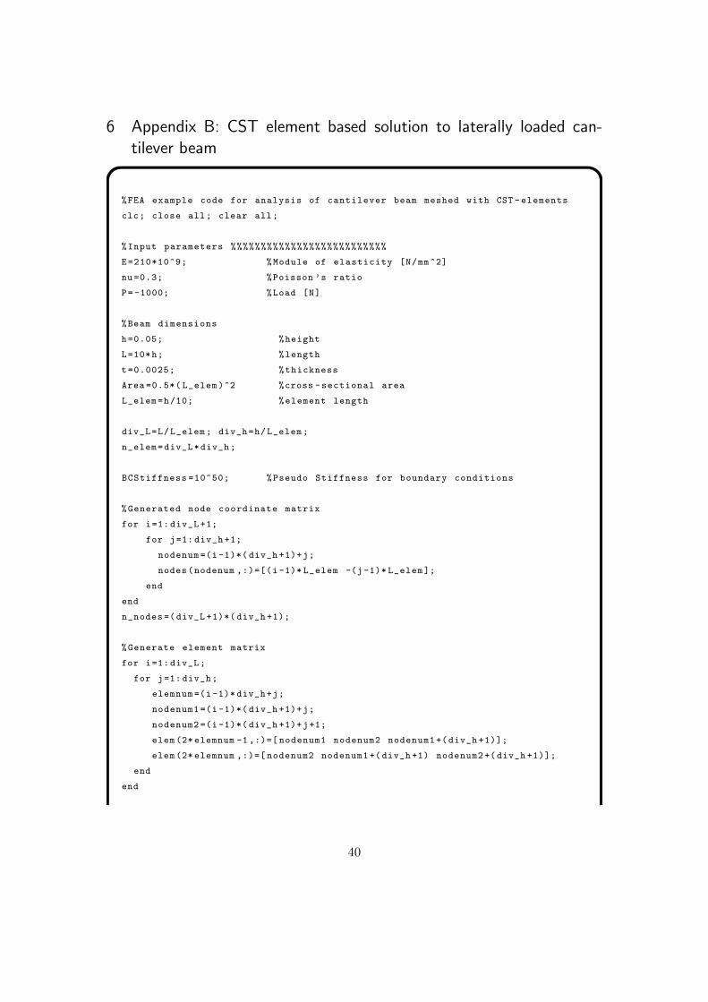
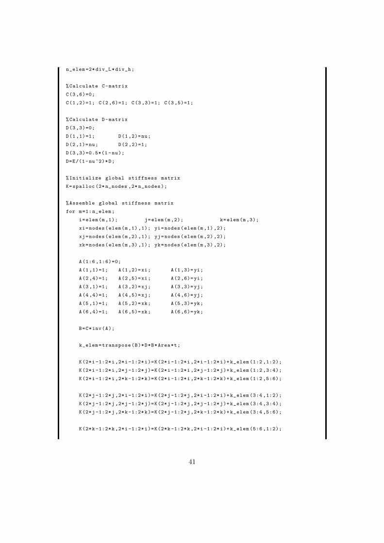
6 Appendix B: CST element based solution to laterally loaded can-tilever beam
%FEA example code for analysis of cantilever beam meshed with CST -elements
clc; close all; clear all;
%Input parameters %%%%%%%%%%%%%%%%%%%%%%%%%%
E=210*10^9; %Module of elasticity [N/mm^2]
nu=0.3; %Poisson ’s ratio
P= -1000; %Load [N]
%Beam dimensions
h=0.05; %height
L=10*h; %length
t=0.0025; %thickness
Area =0.5*( L_elem )^2 %cross -sectional area
L_elem=h/10; %element length
div_L=L/L_elem; div_h=h/L_elem;
n_elem=div_L*div_h;
BCStiffness =10^50; %Pseudo Stiffness for boundary conditions
%Generated node coordinate matrix
for i=1: div_L +1;
for j=1: div_h +1;
nodenum =(i -1)*( div_h +1)+j;
nodes(nodenum ,:)=[(i-1)* L_elem -(j-1)* L_elem ];
end
end
n_nodes =(div_L +1)*( div_h +1);
%Generate element matrix
for i=1: div_L;
for j=1: div_h;
elemnum =(i-1)* div_h+j;
nodenum1 =(i-1)*( div_h +1)+j;
nodenum2 =(i-1)*( div_h +1)+j+1;
elem (2* elemnum -1 ,:)=[ nodenum1 nodenum2 nodenum1 +( div_h +1)];
elem (2* elemnum ,:)=[ nodenum2 nodenum1 +(div_h +1) nodenum2 +(div_h +1)];
end
end
40
n_elem =2* div_L*div_h;
%Calculate C-matrix
C(3 ,6)=0;
C(1 ,2)=1; C(2 ,6)=1; C(3 ,3)=1; C(3 ,5)=1;
%Calculate D-matrix
D(3 ,3)=0;
D(1 ,1)=1; D(1,2)=nu;
D(2 ,1)=nu; D(2 ,2)=1;
D(3 ,3)=0.5*(1 -nu);
D=E/(1-nu^2)*D;
%Initialize global stiffness matrix
K=spalloc (2* n_nodes ,2* n_nodes );
%Assemble global stiffness matrix
for m=1: n_elem;
i=elem(m,1); j=elem(m,2); k=elem(m,3);
xi=nodes(elem(m,1) ,1); yi=nodes(elem(m,1) ,2);
xj=nodes(elem(m,2) ,1); yj=nodes(elem(m,2) ,2);
xk=nodes(elem(m,3) ,1); yk=nodes(elem(m,3) ,2);
A(1:6 ,1:6)=0;
A(1 ,1)=1; A(1,2)=xi; A(1,3)=yi;
A(2 ,4)=1; A(2,5)=xi; A(2,6)=yi;
A(3 ,1)=1; A(3,2)=xj; A(3,3)=yj;
A(4 ,4)=1; A(4,5)=xj; A(4,6)=yj;
A(5 ,1)=1; A(5,2)=xk; A(5,3)=yk;
A(6 ,4)=1; A(6,5)=xk; A(6,6)=yk;
B=C*inv(A);
k_elem=transpose(B)*D*B*Area*t;
K(2*i-1:2*i,2*i -1:2*i)=K(2*i-1:2*i,2*i -1:2*i)+ k_elem (1:2 ,1:2);
K(2*i-1:2*i,2*j -1:2*j)=K(2*i-1:2*i,2*j -1:2*j)+ k_elem (1:2 ,3:4);
K(2*i-1:2*i,2*k -1:2*k)=K(2*i-1:2*i,2*k -1:2*k)+ k_elem (1:2 ,5:6);
K(2*j-1:2*j,2*i -1:2*i)=K(2*j-1:2*j,2*i -1:2*i)+ k_elem (3:4 ,1:2);
K(2*j-1:2*j,2*j -1:2*j)=K(2*j-1:2*j,2*j -1:2*j)+ k_elem (3:4 ,3:4);
K(2*j-1:2*j,2*k -1:2*k)=K(2*j-1:2*j,2*k -1:2*k)+ k_elem (3:4 ,5:6);
K(2*k-1:2*k,2*i -1:2*i)=K(2*k-1:2*k,2*i -1:2*i)+ k_elem (5:6 ,1:2);
41
K(2*k-1:2*k,2*j -1:2*j)=K(2*k-1:2*k,2*j -1:2*j)+ k_elem (5:6 ,3:4);
K(2*k-1:2*k,2*k -1:2*k)=K(2*k-1:2*k,2*k -1:2*k)+ k_elem (5:6 ,5:6);
end
%Generate nodal load vector
F(2* n_nodes )=0;
F(2* n_nodes )=P;
%Set boundary conditions
for m=1:2*( div_h +1);
K(m,m)= BCStiffness;
end
%Solve problem
d=inv(K)*F’;
%Postprocessing , elementwise stress calculations
for m=1: n_elem;
i=elem(m,1); j=elem(m,2); k=elem(m,3);
xi=nodes(elem(m,1) ,1); yi=nodes(elem(m,1) ,2);
xj=nodes(elem(m,2) ,1); yj=nodes(elem(m,2) ,2);
xk=nodes(elem(m,3) ,1); yk=nodes(elem(m,3) ,2);
A(1:6 ,1:6)=0;
A(1 ,1)=1; A(1,2)=xi; A(1,3)=yi;
A(2 ,4)=1; A(2,5)=xi; A(2,6)=yi;
A(3 ,1)=1; A(3,2)=xj; A(3,3)=yj;
A(4 ,4)=1; A(4,5)=xj; A(4,6)=yj;
A(5 ,1)=1; A(5,2)=xk; A(5,3)=yk;
A(6 ,4)=1; A(6,5)=xk; A(6,6)=yk;
H=D*C*inv(A);
dE=[d(2* elem(m,1)-1) d(2* elem(m,1)) d(2* elem(m,2)-1) //
d(2* elem(m,2)) d(2* elem(m,3) -1) d(2* elem(m,3))] ’;
Sigma(m,:)=H*dE;
end
42