Embed Size (px)
Citation preview
Lecture Notes for the courseInvesterings- og Finansieringsteori.
David LandoRolf Poulsen
January 2002

2
Contents
1 Preface 7
2 Introduction 9
2.1 The Role of Financial Markets . . . . . . . . . . . . . . . . . . 10
3 Payment Streams under Certainty 15
3.1 Security markets and arbitrage . . . . . . . . . . . . . . . . . 15
3.2 Zero-coupon bonds and the term structure of interest rates. . . 18
3.3 Annuities, serial loans and bullet bonds. . . . . . . . . . . . . 21
3.4 IRR, NPV and capital budgeting under certainty. . . . . . . . 28
3.4.1 Some rules which are inconsistent with the NPV rule. . 31
3.4.2 Several projects. . . . . . . . . . . . . . . . . . . . . . 32
3.5 Duration, convexity and immunization. . . . . . . . . . . . . . 34
3.5.1 Duration with a flat term structure. . . . . . . . . . . . 34
3.5.2 Relaxing the assumption of a flat term structure. . . . 38
3.5.3 An example . . . . . . . . . . . . . . . . . . . . . . . . 40
4 Arbitrage pricing in a one-period model 43
4.1 An appetizer. . . . . . . . . . . . . . . . . . . . . . . . . . . . 44
4.2 The single period model . . . . . . . . . . . . . . . . . . . . . 46
4.3 The economic intuition . . . . . . . . . . . . . . . . . . . . . 50
5 Arbitrage pricing in the multi-period model 55
5.1 An appetizer . . . . . . . . . . . . . . . . . . . . . . . . . . . 55
5.2 Price processes, trading and arbitrage . . . . . . . . . . . . . . 58
5.3 No arbitrage and price functionals . . . . . . . . . . . . . . . . 63
5.4 Conditional expectations and martingales . . . . . . . . . . . . 65
5.5 Equivalent martingale measures . . . . . . . . . . . . . . . . . 67
5.6 One-period submodels . . . . . . . . . . . . . . . . . . . . . . 72
5.7 The multi-period model on matrix form . . . . . . . . . . . . . 73
3
4 CONTENTS
6 Option pricing 75
6.1 Terminology . . . . . . . . . . . . . . . . . . . . . . . . . . . . 75
6.2 Diagrams, strategies and put-call parity . . . . . . . . . . . . . 76
6.3 Restrictions on option prices . . . . . . . . . . . . . . . . . . . 81
6.4 Binomial models for stock options . . . . . . . . . . . . . . . . 83
6.5 Pricing the European call . . . . . . . . . . . . . . . . . . . . 85
6.6 Hedging the European call . . . . . . . . . . . . . . . . . . . . 86
6.7 Recombining tree representation . . . . . . . . . . . . . . . . . 88
6.8 The binomial model for American puts . . . . . . . . . . . . . 91
6.9 Implied volatility . . . . . . . . . . . . . . . . . . . . . . . . . 92
6.10 Portfolio insurance, implied volatility and crash fears . . . . . 94
6.11 Debt and equity as options on firm value . . . . . . . . . . . . 95
7 The Black-Scholes formula 99
7.1 Black-Scholes as a limit of binomial models . . . . . . . . . . . 99
7.2 The Black-Scholes model . . . . . . . . . . . . . . . . . . . . . 103
7.3 A derivation of the Black-Scholes formula . . . . . . . . . . . . 106
7.3.1 Hedging the call . . . . . . . . . . . . . . . . . . . . . . 110
8 Some notes on term structure modelling 111
8.1 Introduction . . . . . . . . . . . . . . . . . . . . . . . . . . . . 111
8.2 Constructing an arbitrage free model . . . . . . . . . . . . . . 112
8.2.1 Constructing a Q-tree for the short rate that fits theinitial term structure . . . . . . . . . . . . . . . . . . . 115
8.3 On the impossibility of flat shifts of flat term structures . . . . 118
8.4 On forwards and futures . . . . . . . . . . . . . . . . . . . . . 120
8.5 On swap contracts . . . . . . . . . . . . . . . . . . . . . . . . 124
8.6 On expectation hypotheses . . . . . . . . . . . . . . . . . . . . 127
8.7 Why P = Q means risk neutrality . . . . . . . . . . . . . . . . 130
9 Portfolio Theory 133
9.1 The Mathematics of the Efficient Frontier . . . . . . . . . . . 136
9.1.1 The case with no riskfree asset . . . . . . . . . . . . . . 136
9.1.2 The case with a riskfree asset . . . . . . . . . . . . . . 143
9.2 The Capital Asset Pricing Model (CAPM) . . . . . . . . . . 145
9.3 Relevant, but not particularly structured, remarks on CAPM . 151
9.3.1 Systematic and non-systematic risk . . . . . . . . . . . 151
9.3.2 Problems in testing the CAPM . . . . . . . . . . . . . 152
9.3.3 Testing the efficiency of a given portfolio . . . . . . . . 153
CONTENTS 5
10 The APT model 15510.1 Introduction . . . . . . . . . . . . . . . . . . . . . . . . . . . . 15510.2 Exact APT with no noise . . . . . . . . . . . . . . . . . . . . 15510.3 Introducing noise . . . . . . . . . . . . . . . . . . . . . . . . . 15710.4 Factor structure in a model with infinitely many assets . . . . 158
11 On financial decisions of the firm 16511.1 Introduction . . . . . . . . . . . . . . . . . . . . . . . . . . . . 16511.2 ’Undoing’ the firm’s financial decisions . . . . . . . . . . . . . 16611.3 Tax shield . . . . . . . . . . . . . . . . . . . . . . . . . . . . . 16911.4 Bankruptcy costs . . . . . . . . . . . . . . . . . . . . . . . . . 17011.5 Financing positive NPV projects . . . . . . . . . . . . . . . . 170
12 Efficient Capital Markets 17512.1 Excess returns . . . . . . . . . . . . . . . . . . . . . . . . . . . 17612.2 Martingales, random walks and independent increments . . . . 17912.3 Anomalies . . . . . . . . . . . . . . . . . . . . . . . . . . . . . 18112.4 Excess volatility. . . . . . . . . . . . . . . . . . . . . . . . . . 18212.5 Informationally efficient markets are impossible . . . . . . . . 186

6 CONTENTS
Chapter 1
Preface
These notes are intended for the introductory course ’Investerings- og Fi-nansieringsteori’ given in the third year of the joint mathematics-economicsprogram at the University of Copenhagen. At this stage they are still far fromcomplete. The notes (the dominant part of which are written by DL) aimto fill a gap between elementary textbooks such as Copeland and Weston1
or Brealey and Myers2, and more advanced books which require knowledgeof finance theory and often cover continuous-time modelling, such as Duffie3
and Campbell, Lo and MacKinlay4 and Leroy and Werner.5
Except for a brief introduction to the Black-Scholes model, the aim is topresent important parts of the theory of finance through discrete-time modelsemphasizing definitions and setups which prepare the students for the studyof continuous-time models.
At this stage the notes have no historical accounts and hardly referencesany original papers or existing standard textbooks. This will be remedied inlater versions but at this stage, in addition to the books already mentioned,we would like to acknowledge having included things we learned from theclassic Hull 6, the also recommendable Luenberger7, as well as Jarrow and
1T. Copeland and F. Weston: Financial Theory and Corporate Policy2Brealey and Myers: Principles of Corporate Finance.McGraw-Hill 4th ed. 1991.3Duffie, D: Dynamic Asset Pricing Theory.
3rd ed. Princeton 2001.4Campbell, J., A. Lo and A.C. MacKinlay: The Econometrics of Financial Markets.
Princeton 1997.5LeRoy, S. L. and J. Werner: Principles of Financial Economics, Cambridge 2001.6Hull, J.: Options, Futures and Other Derivative Securities. Prentice-Hall. 4th ed.
19997Luenberger, D., ”Investment Science”, Oxford, 1997.
7

8 CHAPTER 1. PREFACE
Turnbull8, and Jensen. 9
8Jarrow R. and S. Turnbull: Derivative Securities.Cincinnati: South-Western (1996).9Jensen, B.A. Rentesregning. DJØFs forlag. 2001.

Chapter 2
Introduction
A student applying for student loans is investing in his or her human capital.Typically, the income of a student is not large enough to cover living expenses,books etc., but the student is hoping that the education will provide futureincome which is more than enough to repay the loans. The governmentsubsidizes students because it believes that the future income generated byhighly educated people will more than compensate for the costs of subsidy,for example through productivity gains and higher tax revenues.
A first time home buyer is typically not able to pay the price of the newhome up front but will have to borrow against future income and using thehouse as collateral.
A company which sees a profitable investment opportunity may not havesufficient funds to launch the project (buy new machines, hire workers) andwill seek to raise capital by issuing stocks and/or borrowing money from abank.
The student, the home buyer and the company are all in need of moneyto invest now and are confident that they will earn enough in the future topay back loans that they might receive.
Conversely, a pension fund receives payments from members and promisesto pay a certain pension once members retire.
Insurance companies receive premiums on insurance contracts and deliv-ers a promise of future payments in the events of property damage or otherunpleasant events which people wish to insure themselves against.
A new lottery millionaire would typically be interested in investing his orher fortune in some sort of assets (government bonds for example) since thiswill provide a larger income than merely saving the money in a mattress.
The pension fund, the insurance company and the lottery winner are alllooking for profitable ways of placing current income in a way which willprovide income in the future.
9
10 CHAPTER 2. INTRODUCTION
A key role of financial markets is to find efficient ways of connectingthe demand for capital with the supply of capital. The examples aboveillustrated the need for economic agents to substitute income intertemporally.An equally important role of financial markets is to allow risk averse agents(such as insurance buyers) to share risk.
In understanding the way financial markets allocate capital we must un-derstand the chief mechanism by which it performs this allocation, namelythrough prices. Prices govern the flow of capital, and in financial marketsinvestors will compare the price of some financial security with its promisedfuture payments. A very important aspect of this comparison is the riskinessof the promised payments. We have an intuitive feeling that it is reason-able for government bonds to give a smaller expected return than stocks inrisky companies, simply because the government is less likely to default. Butexactly how should the relationship between risk and reward (return on aninvestment) be in a well functioning market? Trying to answer that questionis a central part of this course. The best answers delivered so far are in a setof mathematical models developed over the last 40 years or so. One set ofmodels, CAPM and APT, consider expected return and variance on returnas the natural definitions of reward and risk, respectively and tries to answerhow these should be related. Another set of models are based on arbitragepricing, which is a very powerful application of the simple idea, that twosecurities which deliver the same payments should have the same price. Thisis typically illustrated through option pricing models and in the modellingof bond markets, but the methodology actually originated partly in workwhich tried to answer a somewhat different question, which is an essentialpart of financial theory as well: How should a firm finance its investments?Should it issue stocks and/or bonds or maybe something completely differ-ent? How should it (if at all) distribute dividends among shareholders? Theso-called Modigliani-Miller theorems provide a very important starting pointfor studying these issues which currently are by no means resolved.
A historical survey of how finance theory has evolved will probably bemore interesting at the end of the course since we will at that point under-stand versions of the central models of the theory.
But let us start by considering a classical explanation of the significanceof financial markets in a microeconomic setting.
2.1 The Role of Financial Markets
Consider the definition of a private ownership economy as in Debreu (1959):Assume for simplicity that there is only one good and one firm with pro-
2.1. THE ROLE OF FINANCIAL MARKETS 11
duction set Y . The ith consumer is characterized by a consumption set Xi,a preference preordering i, an endowment ωi and shares in the firm θi.Given a price system p, and given a profit maximizing choice of productiony, the firm then has a profit of π(p) = p · y and this profit is distributed toshareholders such that the wealth of the ith consumer becomes
wi = p · ωi + θiπ(p) (2.1)
The definition of an equilibrium in such an economy then has three seem-ingly natural requirements: The firm maximizes profits, consumers maximizeutility subject to their budget constraint and markets clear, i.e. consumptionequals the sum of initial resources and production. But why should the firmmaximize its profits? After all, the firm has no utility function, only con-sumers do. But note that given a price system p, the shareholders of the firmall agree that it is desirable to maximize profits, for the higher profits thelarger the consumers wealth, and hence the larger is the set of feasible con-sumption plans, and hence the larger is the attainable level of utility. In thisway the firm’s production choice is separated from the shareholders’ choiceof consumption. There are many ways in which we could imagine sharehold-ers disagreeing over the firm’s choice of production. Some examples couldinclude cases where the choice of production influences on the consumptionsets of the consumers, or if we relax the assumption of price taking behavior,where the choice of production plan affects the price system and thereby theinitial wealth of the shareholders. Let us, by two examples, illustrate in whatsense the price system changes the behavior of agents.
Example 1 Consider a single agent who is both a consumer and a producer.The agent has an initial endowment e0 > 0 of the date 0 good and has todivide this endowment between consumption at date 0 and investment inproduction of a time 1 good. Assume that only non-negative consumption isallowed. Through investment in production, the agent is able to transforman input of i0 into f(i0) units of date 1 consumption. The agent has autility function U(c0, c1) which we assume is strictly increasing. The agent’sproblem is then to maximize utility of consumption, i.e. to maximize U(c0, c1)subject to the constraints c0 + i0 ≤ e0 and c1 = f(i0) and we may rewritethis problem as
max v(c0) ≡ U(c0, f(e0 − c0))
s.t. c0 ≤ e0
If we impose regularity conditions on the functions f and U (for examplethat they are differentiable and strictly concave and that utility of zero con-sumption in either period is -∞) then we know that at the maximum c∗0 we
12 CHAPTER 2. INTRODUCTION
will have 0 < c∗0 < e0 and v′(c∗0) = 0 i.e.
D1U(c∗0, f(e0 − c∗0)) · 1−D2U(c∗0, f(e0 − c∗0))f′(e0 − c∗0) = 0
where D1 means differentiation after the first variable. Defining i∗0 as theoptimal investment level and c∗1 = f(e0 − c∗0), we see that
f′(i∗0) =
D1U(c∗0, c∗1)
2U(c∗0, c∗1)
and this condition merely says that the marginal rate of substitution in pro-duction is equal to the marginal rate of substitution of consumption.
The key property to note in this example is that what determines theproduction plan in the absence of prices is the preferences for consumptionof the consumer. If two consumers with no access to trade owned shares inthe same firm, but had different preferences and identical initial endowments,they would bitterly disagree on the level of the firm’s investment.
Example 2 Now consider the setup of the previous example but assumethat a price system (p0, p1) (whose components are strictly positive) givesthe consumer an additional means of transferring date 0 wealth to date1 consumption. Note that by selling one unit of date 0 consumption theagent acquires p0
p1units of date 1 consumption, and we define 1 + r = p0
p1. The
initial endowment must now be divided between three parts: consumption atdate 0 c0, input into production i0 and s0 which is sold in the market andwhose revenue can be used to purchase date 1 consumption in the market.
With this possibility the agent’s problem becomes that of maximizingU(c0, c1) subject to the constraints
c0 + i0 + s0 ≤ e0
c1 ≤ f(i0) + (1 + r)s0
and with monotonicity constraints the inequalities may be replaced by equal-ities. Note that the problem then may be reduced to having two decisionvariables c0 and i0 and maximizing
v(c0, i0) ≡ U(c0, f(i0) + (1 + r)(e0 − c0 − i0)).
Again we may impose enough regularity conditions on U (strict concavity,twice differentiability, strong aversion to zero consumption) to ensure that itattains its maximum in an interior point of the set of feasible pairs (c0, i0)and that at this point the gradient of v is zero, i.e.
D1U(c∗0, c∗1) · 1−D2U(c∗0, f(i∗0) + (1 + r)(e0 − c∗0 − i∗0))(1 + r) = 0
D2U(c∗0, f(i∗0) + (1 + r)(e0 − c∗0 − i∗0))(f′(i∗0)− (1 + r)) = 0
2.1. THE ROLE OF FINANCIAL MARKETS 13
With the assumption of strictly increasing U, the only way the second equalitycan hold, is if
f′(i∗0) = (1 + r)
and the first equality holds if
D1U(c∗0, c∗1)
D2U(c∗0, c∗1)
= (1 + r)
We observe two significant features:First, the production decision is independent of the utility function of
the agent. Production is chosen to a point where the marginal benefit ofinvesting in production is equal to the ’interest rate’ earned in the market.The consumption decision is separate from the production decision and themarginal condition is provided by the market price. In such an environmentwe have what is known as Fisher Separation where the firm’s decision isindependent of the shareholder’s utility functions. Such a setup rests criti-cally on the assumptions of the perfect competitive markets where there isprice taking behavior and a market for both consumption goods at date 0.Whenever we speak of firms having the objective of maximizing sharehold-ers’ wealth we are assuming an economy with a setup similar to that of theprivate ownership economy of which we may think of the second example asa very special case.
Second, the solution to the maximization problem will typically have ahigher level of utility for the agent at the optimal point: Simply note thatany feasible solution to the first maximization problem is also a solutionto the second. This is an improvement which we take as a ’proof’ of thesignificance of the existence of markets. If we consider a private ownershipeconomy equilibrium, the equilibrium price system will see to that consumersand producers coordinate their activities simply by following the price systemand they will obtain higher utility than if each individual would act withouta price system as in example 1.

14 CHAPTER 2. INTRODUCTION
Chapter 3
Payment Streams underCertainty
3.1 Security markets and arbitrage
In this section we consider a very simple setup with no uncertainty. Thereare three reasons that we do this:
First, the terminology of bond markets is conveniently introduced in thissetting, for even if there were uncertainty in our model, bonds would becharacterized by having payments whose size at any date are constant andknown in advance.
Second, the classical NPV rule of capital budgeting is easily understoodin this framework.
And finally, the mathematics introduced in this section will be extremelyuseful in later chapters as well.
A note on notation: If v ∈ RN is a vector the following conventions areused:
• v ≥ 0 means that all of v′s coordinates are non-negative. This we wouldalso write as v ∈ RN+ ∪ 0 .
• v > 0 means that v ≥ 0 and that at least one coordinate is strictlypositive. This we would also write as v ∈ RN+ .
• v 0 means that every coordinate is strictly positive. This we wouldalso write as v ∈ RN++.
Throughout we use v> to denote the transpose of the vector v. Vectorswithout the transpose sign are always thought of as column vectors.
15
16 CHAPTER 3. PAYMENT STREAMS UNDER CERTAINTY
We now consider a model for a financial market with T+1 dates: 0, 1, ..., Tand no uncertainty.
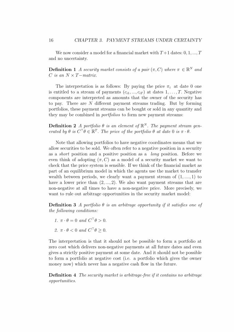
Definition 1 A security market consists of a pair (π,C) where π ∈ RN andC is an N × T−matrix.
The interpretation is as follows: By paying the price πi at date 0 oneis entitled to a stream of payments (ci1, ..., ciT ) at dates 1, . . . , T. Negativecomponents are interpreted as amounts that the owner of the security hasto pay. There are N different payment streams trading. But by formingportfolios, these payment streams can be bought or sold in any quantity andthey may be combined in portfolios to form new payment streams:
Definition 2 A portfolio θ is an element of RN . The payment stream gen-erated by θ is C>θ ∈ RT . The price of the portfolio θ at date 0 is π · θ.
Note that allowing portfolios to have negative coordinates means that weallow securities to be sold. We often refer to a negative position in a securityas a short position and a positive position as a long position. Before weeven think of adopting (π,C) as a model of a security market we want tocheck that the price system is sensible. If we think of the financial market aspart of an equilibrium model in which the agents use the market to transferwealth between periods, we clearly want a payment stream of (1, ...., 1) tohave a lower price than (2, ..., 2). We also want payment streams that arenon-negative at all times to have a non-negative price. More precisely, wewant to rule out arbitrage opportunities in the security market model:
Definition 3 A portfolio θ is an arbitrage opportunity if it satisfies one ofthe following conditions:
1. π · θ = 0 and C>θ > 0.
2. π · θ < 0 and C>θ ≥ 0.
The interpretation is that it should not be possible to form a portfolio atzero cost which delivers non-negative payments at all future dates and evengives a strictly positive payment at some date. And it should not be possibleto form a portfolio at negative cost (i.e. a portfolio which gives the ownermoney now) which never has a negative cash flow in the future.
Definition 4 The security market is arbitrage-free if it contains no arbitrageopportunities.
3.1. SECURITY MARKETS AND ARBITRAGE 17
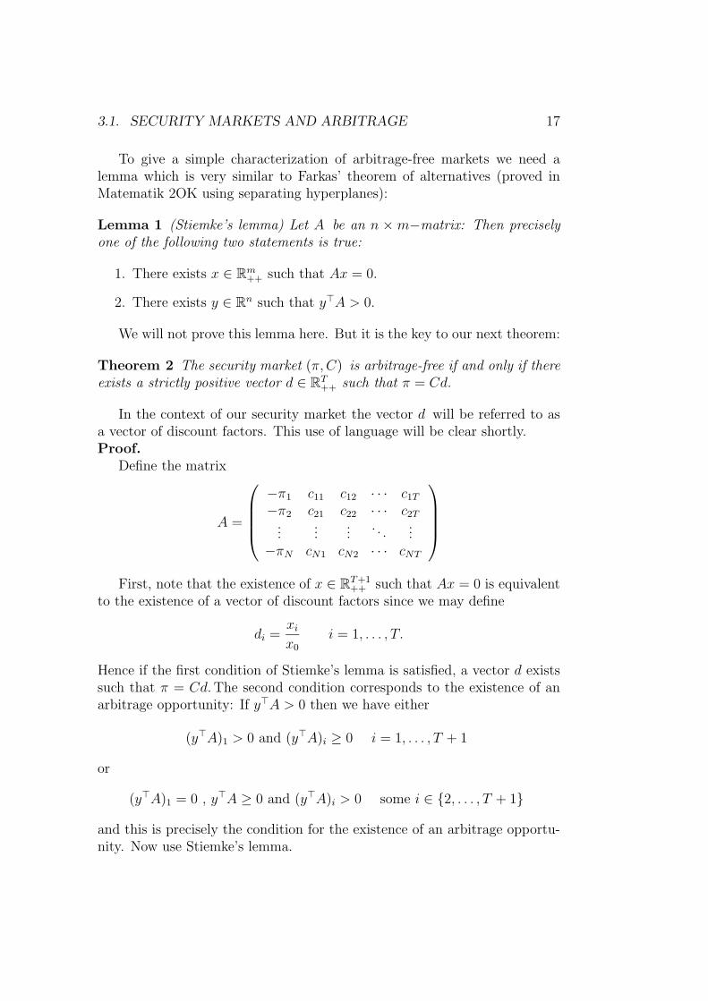
To give a simple characterization of arbitrage-free markets we need alemma which is very similar to Farkas’ theorem of alternatives (proved inMatematik 2OK using separating hyperplanes):
Lemma 1 (Stiemke’s lemma) Let A be an n ×m−matrix: Then preciselyone of the following two statements is true:
1. There exists x ∈ Rm++ such that Ax = 0.
2. There exists y ∈ Rn such that y>A > 0.
We will not prove this lemma here. But it is the key to our next theorem:
Theorem 2 The security market (π,C) is arbitrage-free if and only if thereexists a strictly positive vector d ∈ RT++ such that π = Cd.
In the context of our security market the vector d will be referred to asa vector of discount factors. This use of language will be clear shortly.Proof.
Define the matrix
A =
−π1 c11 c12 · · · c1T
−π2 c21 c22 · · · c2T...
......
. . ....
−πN cN1 cN2 · · · cNT
First, note that the existence of x ∈ RT+1
++ such that Ax = 0 is equivalentto the existence of a vector of discount factors since we may define
di =xix0
i = 1, . . . , T.
Hence if the first condition of Stiemke’s lemma is satisfied, a vector d existssuch that π = Cd.The second condition corresponds to the existence of anarbitrage opportunity: If y>A > 0 then we have either
(y>A)1 > 0 and (y>A)i ≥ 0 i = 1, . . . , T + 1
or
(y>A)1 = 0 , y>A ≥ 0 and (y>A)i > 0 some i ∈ 2, . . . , T + 1
and this is precisely the condition for the existence of an arbitrage opportu-nity. Now use Stiemke’s lemma.
18 CHAPTER 3. PAYMENT STREAMS UNDER CERTAINTY
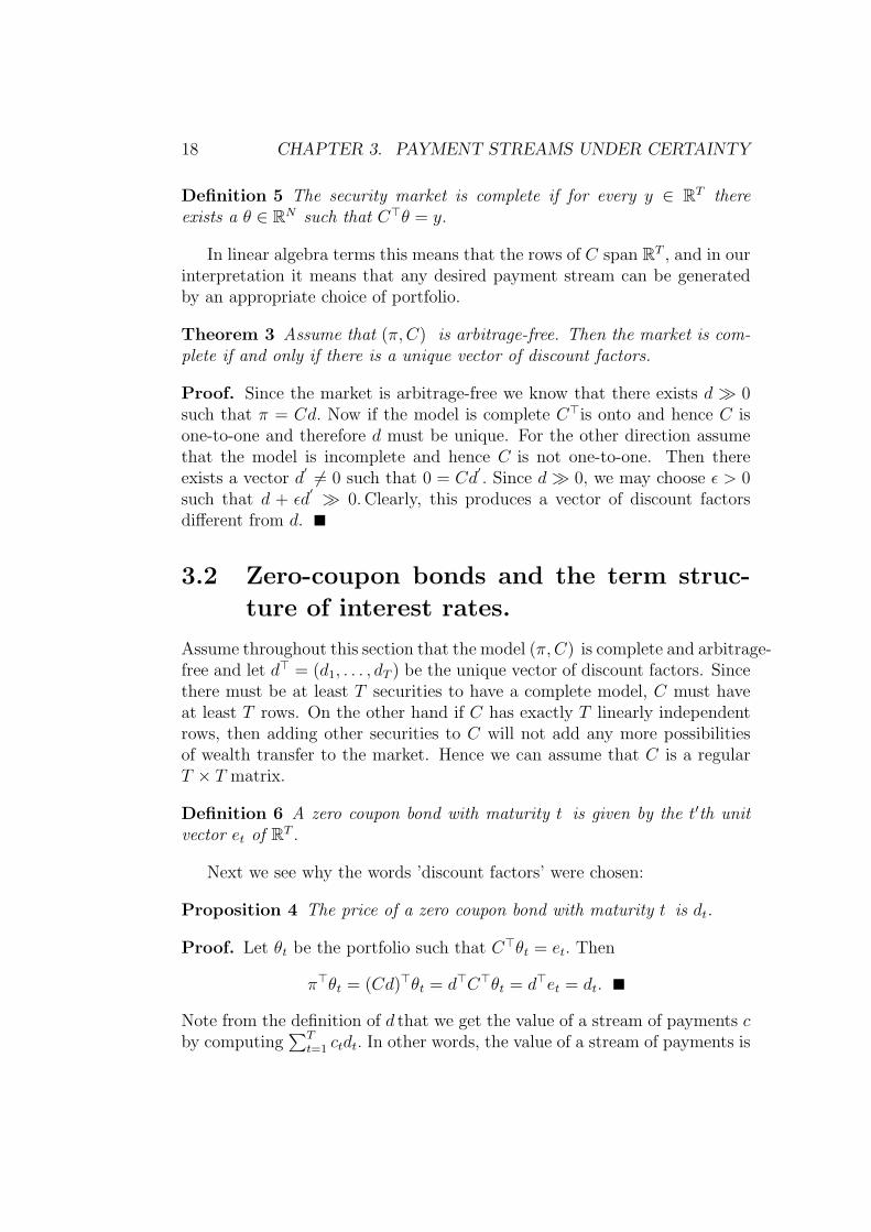
Definition 5 The security market is complete if for every y ∈ RT thereexists a θ ∈ RN such that C>θ = y.
In linear algebra terms this means that the rows of C span RT , and in ourinterpretation it means that any desired payment stream can be generatedby an appropriate choice of portfolio.
Theorem 3 Assume that (π,C) is arbitrage-free. Then the market is com-plete if and only if there is a unique vector of discount factors.
Proof. Since the market is arbitrage-free we know that there exists d 0such that π = Cd. Now if the model is complete C>is onto and hence C isone-to-one and therefore d must be unique. For the other direction assumethat the model is incomplete and hence C is not one-to-one. Then thereexists a vector d
′ 6= 0 such that 0 = Cd′. Since d 0, we may choose ε > 0
such that d + εd′ 0.Clearly, this produces a vector of discount factors
different from d.
3.2 Zero-coupon bonds and the term struc-
ture of interest rates.
Assume throughout this section that the model (π,C) is complete and arbitrage-free and let d> = (d1, . . . , dT ) be the unique vector of discount factors. Sincethere must be at least T securities to have a complete model, C must haveat least T rows. On the other hand if C has exactly T linearly independentrows, then adding other securities to C will not add any more possibilitiesof wealth transfer to the market. Hence we can assume that C is a regularT × T matrix.
Definition 6 A zero coupon bond with maturity t is given by the t′th unitvector et of RT .
Next we see why the words ’discount factors’ were chosen:
Proposition 4 The price of a zero coupon bond with maturity t is dt.
Proof. Let θt be the portfolio such that C>θt = et. Then
π>θt = (Cd)>θt = d>C>θt = d>et = dt.
Note from the definition of d that we get the value of a stream of payments cby computing
∑Tt=1 ctdt. In other words, the value of a stream of payments is
3.2. ZERO-COUPON BONDS AND THE TERM STRUCTURE OF INTEREST RATES.19
obtained by discounting back the individual components. There is nothingin our definition of d which prevents ds > dt even when s > t,but in themodels we will consider this will not be relevant: It is safe to think of dt asdecreasing in t corresponding to the idea that the longer the maturity of azero coupon bond, the smaller is its value at time 0.
From the discount factors we may derive various types of interest rateswhich are essential in the study of bond markets.:
Definition 7 The spot rate at date 0 is given by
r0 =1
d1
− 1.
The (one-period) time t− forward rate at date 0, is equal to
f(0, t) =dtdt+1
− 1,
where d0 = 1 by convention.
The interpretation of the spot rate should be straightforward: Buying 1d1
units of a maturity 1 zero coupon bond costs 1d1d1 = 1 at date 0 and gives a
payment at date 1 of 1d1
= 1 + r0.The forward rate tells us the rate at which we may agree at date 0 to
borrow (or lend) between dates t and t+1. To see this, consider the followingstrategy at time 0 :
• Sell 1 zero coupon bond with maturity t.
• Buy dtdt+1
zero coupon bonds with maturity t+ 1.
Note that the amount raised by selling precisely matches the amount usedfor buying and hence the cash flow from this strategy at time 0 is 0. Nowconsider what happens if the positions are held to the maturity date of thebonds:
At date t the cash flow is then −1 and at date t + 1 the cash flow isdtdt+1
= 1 + f(0, t).
Definition 8 The yield (or yield to maturity) at time 0 of a zero couponbond with maturity t is given as
y(0, t) =
(1
dt
) 1t
− 1.
20 CHAPTER 3. PAYMENT STREAMS UNDER CERTAINTY
Note thatdt(1 + y(0, t))t = 1.
and that one may therefore think of the yield as an ’average interest rate’earned on a zero coupon bond. In fact, the yield is a geometric average offorward rates:
1 + y(0, t) = ((1 + f(0, 0)) · · · (1 + f(0, t− 1)))1t
Definition 9 The term structure of interest rates (or the yield structure ofinterest rates) at date 0 is given by (y(0, 1), . . . , y(0, T )).
Note that if we have any one of the vector of yields, the vector of forwardrates and the vector of discount factors, we may determine the other two.Therefore we could equally well define a term structure of forward rates anda term structure of discount factors. In these notes unless otherwise stated,we think of the term structure of interest rates as the yields of zero couponbonds as a function of time to maturity. It is important to note that the termstructure of interest rate depicts yields of zero coupon bonds. We do howeveralso speak of yields on securities which have no negative payments(and somestrictly positive payments):
Definition 10 The yield (or yield to maturity) of a security c> = (c1, . . . , cT )with c > 0 and price π is the unique solution y > −1 of the equation
π =T∑i=1
ci(1 + y)i
.
Example 3 (Compounding Periods) In most of the analysis in this chap-ter the time is “stylized”; it is measured in some unit (which we think of andrefer to as “years”) and cash-flows occur at dates 0, 1, 2, . . . , T. But itis often convenient (and not hard) to work with dates that are not integermultiples of the fundamental time-unit. We quote interest rates in units ofyears−1 (“per year’), but to any interest rate there should be a number, m,associated stating how often the interest is compounded. By this we meanthe following: If you invest 1 $ for n years at the m-compounded rate rm youend up with (
1 +rmm
)mn. (3.1)
The standard example: If you borrow 1$ in the bank, a 12% interest ratemeans they will add 1% to you debt each month (i.e. m = 12) and youwill end up paying back 1.1268 $ after a year, while if you make a deposit,
3.3. ANNUITIES, SERIAL LOANS AND BULLET BONDS. 21
they will add 12% after a year (i.e. m = 1) and you will of course get 1.12$back after one year. If we keep rm and n fixed in (3.1) (and then drop them-subscript) and and let m tend to infinity, it is well known that we get:
limm→∞
(1 +
r
m
)mn= enr,
and in this case we will call r the continuously compounded interest rate. Inother words: If you invest 1 $ and the continuously compounded rate rc fora period af lenght t, you will get back etrc . Note also that a continuouslycompounded rate rc can be used to find (uniquely for any m) rm such that1 $ invested at m-compounding corresonds to 1 $ invested at continuouscompounding, i.e. (
1 +rmm
)m= erc .
This means that in order to avoid confusion – even in discrete models –there is much to be said in favor of quoting interest rates on a continuouslycompounded basis. But then again, in the highly stylized discrete modelsit would be pretty artificial, so we will not do it (rather it will always bem = 1).
3.3 Annuities, serial loans and bullet bonds.
Typically, zero-coupon bonds of all maturities do not trade in financial mar-kets and one therefore has to deduce prices of zero-coupon bonds from othertypes of bonds trading in the market. Three of the most common types ofbonds which do trade in most bond markets are annuities, serial loans andbullet bonds. We now show how knowing to which of these three types abond belongs and knowing three characteristics, namely the maturity, theprincipal and the coupon rate, will enable us to determine the bond’s cashflow completely.
Let the principal or face value of the bond be denoted F. Payments on thebond start at date 1 and continue to the time of the bond’s maturity, whichwe denote τ . The payments are denoted ct. We think of the principal of abond with coupon rate R and payments c1, . . . , cτ as satisfying the followingdifference equation:
pt = (1 +R)pt−1 − ct t = 1, . . . , τ , (3.2)
with the boundary conditions p0 = F and pτ = 0.Think of pt as the remaining principal right after a payment at date
t has been made. For accounting and tax purposes and also as a helpful tool
22 CHAPTER 3. PAYMENT STREAMS UNDER CERTAINTY
in designing particular types of bonds, it is useful to split payments into apart which serves as reduction of principal and one part which is seen as aninterest payment. We define the reduction in principal at date t as
δt = pt−1 − pt
and the interest payment as
it = Rpt−1 = ct − δt.
Definition 11 An annuity with maturity τ , principal F and coupon rate Ris a bond whose payments are constant between date 1 and date τ and whoseprincipal evolves according to (3.2).
Note that with constant payments we may write the remaining principalat time t as
pt = (1 +R)tF − ct−1∑j=0
(1 +R)j t = 1, 2, . . . , τ .
To satisfy the boundary condition pτ = 0 we must therefore have
F − cτ−1∑j=0
(1 +R)j−τ = 0
i.e.
c = F
(τ−1∑j=0
(1 +R)j−τ
)−1
= FR(1 +R)τ
(1 +R)τ − 1.
It is common to use the shorthand notation
αneR = (“Alfahage”) =(1 +R)n − 1
R(1 +R)n.
Having found what the size of the payment must be we may derive the interestand the deduction of principal as well:
Let us calculate the size of the payments and see how they split intodeduction of principal and interest payments.
3.3. ANNUITIES, SERIAL LOANS AND BULLET BONDS. 23
First, we derive an expression for the remaining principal:
pt = (1 +R)tF − F
ατeR
t−1∑j=0
(1 +R)j
=F
ατeR
((1 +R)tατeR −
(1 +R)t − 1
R
)=
F
ατeR
((1 +R)τ − 1
R(1 +R)τ−t− (1 +R)τ − (1 +R)τ−t
R(1 +R)τ−t
)=
F
ατeRατ−teR.
This gives us the interest payment and the deduction immediately for theannuity:
it = RF
ατeRατ−t+1eR
δt =F
ατeR(1−Rατ−t+1eR).
Definition 12 A bullet bond1 with maturity τ ,principal F and coupon rateR is characterized by having it = ct for t = 1, . . . , τ − 1 and cτ = (1 +R)F.
The fact that we have no reduction in principal before τ forces us to havect = RF for all t < τ.
Definition 13 A serial bond with maturity τ , principal F and coupon rateR is characterized by having δt constant for all t = 1, . . . , τ .
Since the deduction in principal is constant every period and we must havepτ = 0, it is clear that δt = F
τfor t = 1, . . . , τ . From this it is straightforward
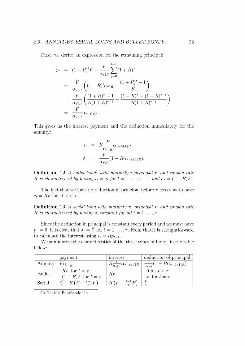
to calculate the interest using it = Rpt−1.We summarize the characteristics of the three types of bonds in the table
below:
payment interest deduction of principalAnnuity Fα−1
τeR R FατeR
ατ−t+1eRF
ατeR(1−Rατ−t+1eR)
BulletRF for t < τ(1 +R)F for t = τ
RF0 for t < τF for t = τ
Serial Fτ
+R(F − t−1
τF)
R(F − t−1
τF)
Fτ
1In Danish: Et staende lan
24 CHAPTER 3. PAYMENT STREAMS UNDER CERTAINTY
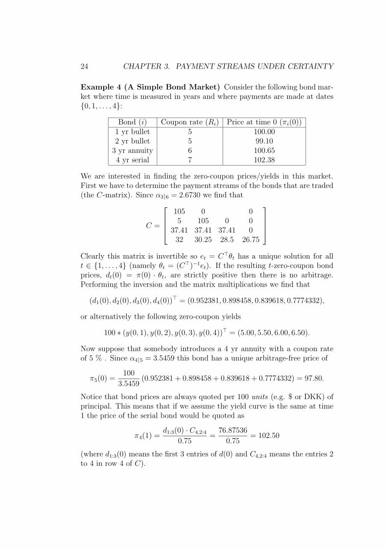
Example 4 (A Simple Bond Market) Consider the following bond mar-ket where time is measured in years and where payments are made at dates0, 1, . . . , 4:
Bond (i) Coupon rate (Ri) Price at time 0 (πi(0))1 yr bullet 5 100.002 yr bullet 5 99.10
3 yr annuity 6 100.654 yr serial 7 102.38
We are interested in finding the zero-coupon prices/yields in this market.First we have to determine the payment streams of the bonds that are traded(the C-matrix). Since α3e6 = 2.6730 we find that
C =
105 0 05 105 0 0
37.41 37.41 37.41 032 30.25 28.5 26.75
Clearly this matrix is invertible so et = C>θt has a unique solution for allt ∈ 1, . . . , 4 (namely θt = (C>)−1et). If the resulting t-zero-coupon bondprices, dt(0) = π(0) · θt, are strictly positive then there is no arbitrage.Performing the inversion and the matrix multiplications we find that
(d1(0), d2(0), d3(0), d4(0))> = (0.952381, 0.898458, 0.839618, 0.7774332),
or alternatively the following zero-coupon yields
100 ∗ (y(0, 1), y(0, 2), y(0, 3), y(0, 4))> = (5.00, 5.50, 6.00, 6.50).
Now suppose that somebody introduces a 4 yr annuity with a coupon rateof 5 % . Since α4e5 = 3.5459 this bond has a unique arbitrage-free price of
π5(0) =100
3.5459(0.952381 + 0.898458 + 0.839618 + 0.7774332) = 97.80.
Notice that bond prices are always quoted per 100 units (e.g. $ or DKK) ofprincipal. This means that if we assume the yield curve is the same at time1 the price of the serial bond would be quoted as
π4(1) =d1:3(0) · C4,2:4
0.75=
76.87536
0.75= 102.50
(where d1:3(0) means the first 3 entries of d(0) and C4,2:4 means the entries 2to 4 in row 4 of C).
3.3. ANNUITIES, SERIAL LOANS AND BULLET BONDS. 25
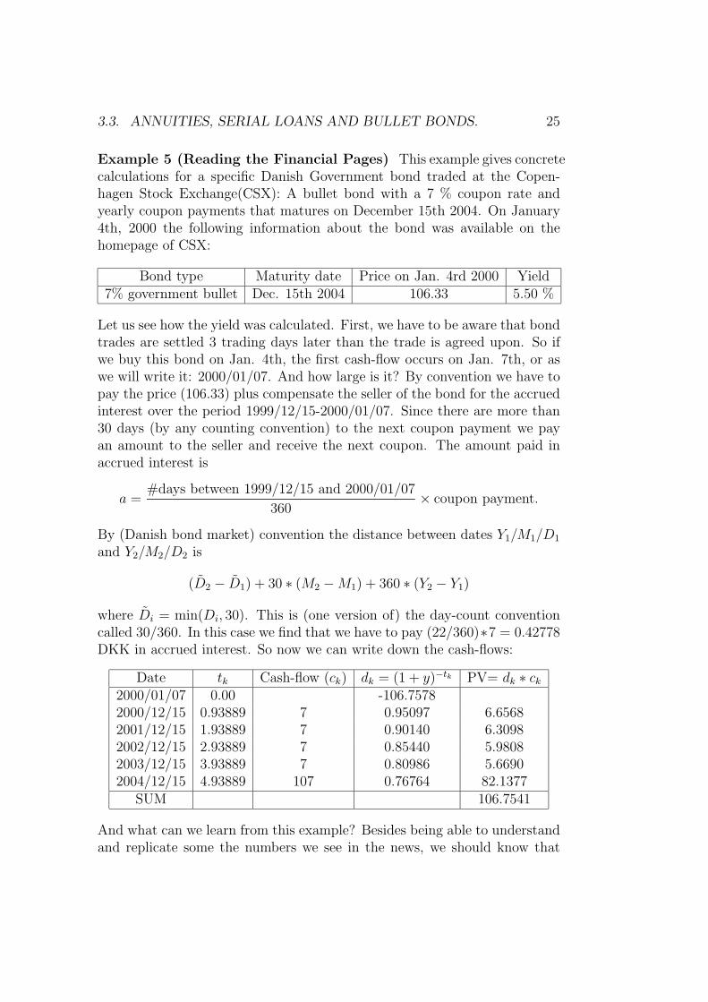
Example 5 (Reading the Financial Pages) This example gives concretecalculations for a specific Danish Government bond traded at the Copen-hagen Stock Exchange(CSX): A bullet bond with a 7 % coupon rate andyearly coupon payments that matures on December 15th 2004. On January4th, 2000 the following information about the bond was available on thehomepage of CSX:
Bond type Maturity date Price on Jan. 4rd 2000 Yield7% government bullet Dec. 15th 2004 106.33 5.50 %
Let us see how the yield was calculated. First, we have to be aware that bondtrades are settled 3 trading days later than the trade is agreed upon. So ifwe buy this bond on Jan. 4th, the first cash-flow occurs on Jan. 7th, or aswe will write it: 2000/01/07. And how large is it? By convention we have topay the price (106.33) plus compensate the seller of the bond for the accruedinterest over the period 1999/12/15-2000/01/07. Since there are more than30 days (by any counting convention) to the next coupon payment we payan amount to the seller and receive the next coupon. The amount paid inaccrued interest is
a =#days between 1999/12/15 and 2000/01/07
360× coupon payment.
By (Danish bond market) convention the distance between dates Y1/M1/D1
and Y2/M2/D2 is
(D2 − D1) + 30 ∗ (M2 −M1) + 360 ∗ (Y2 − Y1)
where Di = min(Di, 30). This is (one version of) the day-count conventioncalled 30/360. In this case we find that we have to pay (22/360)∗7 = 0.42778DKK in accrued interest. So now we can write down the cash-flows:
Date tk Cash-flow (ck) dk = (1 + y)−tk PV= dk ∗ ck2000/01/07 0.00 -106.75782000/12/15 0.93889 7 0.95097 6.65682001/12/15 1.93889 7 0.90140 6.30982002/12/15 2.93889 7 0.85440 5.98082003/12/15 3.93889 7 0.80986 5.66902004/12/15 4.93889 107 0.76764 82.1377
SUM 106.7541
And what can we learn from this example? Besides being able to understandand replicate some the numbers we see in the news, we should know that
26 CHAPTER 3. PAYMENT STREAMS UNDER CERTAINTY
bond markets have a variety of conventions that are not very homogeneous(settlement takes place after 3 days in Denmark, but after 7 in Euroland;banks typically use actual days when counting; the convention 30/360 doesnot mean the same in Europe and the U.S., . . .) Of course we are not in-terested in learning the conventions in this (or any?) course, but we mustrealize that they can be of great practical importance (especially since bondmarket transactions can be extremely large).
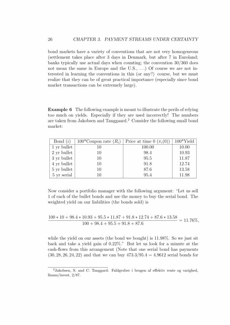
Example 6 The following example is meant to illustrate the perils of relyingtoo much on yields. Especially if they are used incorrectly! The numbersare taken from Jakobsen and Tanggaard.2 Consider the following small bondmarket:
Bond (i) 100*Coupon rate (Ri) Price at time 0 (πi(0)) 100*Yield1 yr bullet 10 100.00 10.002 yr bullet 10 98.4 10.933 yr bullet 10 95.5 11.874 yr bullet 10 91.8 12.745 yr bullet 10 87.6 13.585 yr serial 10 95.4 11.98
Now consider a portfolio manager with the following argument: “Let us sell1 of each of the bullet bonds and use the money to buy the serial bond. Theweighted yield on our liabilities (the bonds sold) is
100 ∗ 10 + 98.4 ∗ 10.93 + 95.5 ∗ 11.87 + 91.8 ∗ 12.74 + 87.6 ∗ 13.58
100 + 98.4 + 95.5 + 91.8 + 87.6= 11.76%,
while the yield on our assets (the bond we bought) is 11.98%. So we just sitback and take a yield gain of 0.22%.” But let us look for a minute at thecash-flows from this arrangement (Note that one serial bond has payments(30, 28, 26, 24, 22) and that we can buy 473.3/95.4 = 4.9612 serial bonds for
2Jakobsen, S. and C. Tanggard: Faldgruber i brugen af effektiv rente og varighed,finans/invest, 2/87.
3.3. ANNUITIES, SERIAL LOANS AND BULLET BONDS. 27
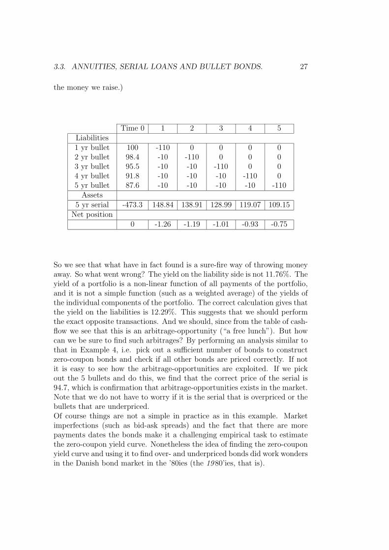
the money we raise.)
Time 0 1 2 3 4 5Liabilities1 yr bullet 100 -110 0 0 0 02 yr bullet 98.4 -10 -110 0 0 03 yr bullet 95.5 -10 -10 -110 0 04 yr bullet 91.8 -10 -10 -10 -110 05 yr bullet 87.6 -10 -10 -10 -10 -110
Assets5 yr serial -473.3 148.84 138.91 128.99 119.07 109.15
Net position0 -1.26 -1.19 -1.01 -0.93 -0.75
So we see that what have in fact found is a sure-fire way of throwing moneyaway. So what went wrong? The yield on the liability side is not 11.76%. Theyield of a portfolio is a non-linear function of all payments of the portfolio,and it is not a simple function (such as a weighted average) of the yields ofthe individual components of the portfolio. The correct calculation gives thatthe yield on the liabilities is 12.29%. This suggests that we should performthe exact opposite transactions. And we should, since from the table of cash-flow we see that this is an arbitrage-opportunity (“a free lunch”). But howcan we be sure to find such arbitrages? By performing an analysis similar tothat in Example 4, i.e. pick out a sufficient number of bonds to constructzero-coupon bonds and check if all other bonds are priced correctly. If notit is easy to see how the arbitrage-opportunities are exploited. If we pickout the 5 bullets and do this, we find that the correct price of the serial is94.7, which is confirmation that arbitrage-opportunities exists in the market.Note that we do not have to worry if it is the serial that is overpriced or thebullets that are underpriced.Of course things are not a simple in practice as in this example. Marketimperfections (such as bid-ask spreads) and the fact that there are morepayments dates the bonds make it a challenging empirical task to estimatethe zero-coupon yield curve. Nonetheless the idea of finding the zero-couponyield curve and using it to find over- and underpriced bonds did work wondersin the Danish bond market in the ’80ies (the 19 80’ies, that is).
28 CHAPTER 3. PAYMENT STREAMS UNDER CERTAINTY
3.4 IRR, NPV and capital budgeting under
certainty.
The definition of internal rate of return (IRR) is the same as that of yield,but we use it on arbitrary cash flows, i.e. on securities which may havenegative cash flows as well:
Definition 14 An internal rate of return of a security (c1, . . . , cT ) with priceπ 6= 0 is a solution y > −1 of the equation
π =T∑i=1
ci(1 + y)i
.
Hence the definitions of yield and internal rate of return are identical forpositive cash flows. It is easy to see that for securities whose future paymentsare both positive and negative we may have several IRRs. This is one reasonthat one should be very careful interpreting and using this measure at allwhen comparing cash flows. We will see below that there are even moreserious reasons. When judging whether a certain cash flow is ’attractive’ thecorrect measure to use is Net Present Value:
Definition 15 The PV and NPV of security (c1, . . . , cT ) with price c0 givena term structure (y(0, 1), . . . , y(0, T )) are defined as
PV (c) =T∑i=1
ci(1 + y(0, i))i
NPV (c) =T∑i=1
ci(1 + y(0, i))i
− c0
Next, we will see how these concepts are used in deciding how to invest undercertainty.
Assume throughout this section that we have a complete security marketas defined in the previous section. Hence a unique discount function d isgiven as well as the associated concepts of interest rates and yields. We lety denote the term structure of interest rates and use the short hand notationyi for y(0, i).
In capital budgeting we analyze how firms should invest in projects whosepayoffs are represented by cash flows. Whereas we assumed in the securitymarket model that a given security could be bought or sold in any quantity
3.4. IRR, NPV AND CAPITAL BUDGETING UNDER CERTAINTY. 29
desired, we will use the term project more restrictively: We will say that theproject is scalable by a factor λ 6= 1 if it is possible to start a project whichproduces the cash flow λc by paying λc0 initially. A project is not scalableunless we state this explicitly and we will not consider any negative scaling.
In a complete financial market an investor who needs to decide on onlyone project faces a very simple decision: Accept the project if and only ifit has positive NPV. We will see why this is shortly. Accepting this factwe will see examples of some other criteria which are generally inconsistentwith the NPV criterion. We will also note that when a collection of projectsare available capital budgeting becomes a problem of maximizing NPV overthe range of available projects. The complexity of the problem arises fromthe constraints that we impose on the projects. The available projects maybe non-scalable or scalable up to a certain point, they may be mutuallyexclusive (i.e. starting one project excludes starting another), we may imposerestrictions on the initial outlay that we will allow the investor to make(representing limited access to borrowing in the financial market), we mayassume that a project may be repeated once it is finished and so on. In allcases our objective is simple: Maximize NPV.
First, let us note why looking at NPV is a sensible thing to do:
Proposition 5 Given a cash flow c = (c1, . . . , cT ) and given c0 such thatNPV (c0; c) < 0. Then there exists a portfolio θ of securities whose price isc0 and whose payoff satisfies
C>θ >
c1...cT
.
Conversely, if NPV (c0; c) > 0, then every θ with C> θ = c satisfies π>θ > c0.
Proof. Since the security market is complete, there exists a portfolio θc suchthat C>θc = c. Now π>θc < c0 (why?), hence we may form a new portfolio byinvesting the amount c0 − π>θc in some zero coupon bond (e1, say) and also
invest in θc. This generates a stream of payments equal to C>θc+ (c0−π>θc)d1
e1 >c and the cost is c0 by construction. The second part is left as an exercise!TCIMACRO
The interpretation of this lemma is the following: One should never accepta project with negative NPV since a strictly larger cash flow can be obtainedat the same initial cost by trading in the capital market. On the other hand,a positive NPV project generates a cash flow at a lower cost than the costof generating the same cash flow in the capital market. It might seem that

30 CHAPTER 3. PAYMENT STREAMS UNDER CERTAINTY
this generates an arbitrage opportunity since we could buy the project andsell the corresponding future cash flow in the capital market generating aprofit at time 0. However, we insist on relating the term arbitrage to thecapital market only. Projects should be thought of as ’endowments’: Firmshave an available range of projects. By choosing the right projects the firmsmaximize the value of these ’endowments’.
Some times when performing NPV−calculations, we assume that ’theterm structure is flat’ . What this means is that the discount function hasthe particularly simple form
dt =1
(1 + r)t
for some constant r, which we will usually assume to be non-negative, al-though our model only guarantees that r > −1 in an arbitrage-free market.A flat term structure is very rarely observed in practice - a typical real worldterm structure will be upward sloping: Yields on long maturity zero couponbonds will be greater than yields on short bonds. Reasons for this will bediscussed once we model the term structure and its evolution over time -a task which requires the introduction of uncertainty to be of any interest.When the term structure is flat then evaluating the NPV of a project havinga constant cash flow is easily done by summing the geometric series. Thepresent value of n payments starting at date 1, ending at date n each of sizec, is
n∑i=1
cdi = cdn−1∑i=0
di = cd1− dn
1− d, d 6= 1
Another classical formula concerns the present value of a geometrically grow-ing payment stream (c, c(1 + g), . . . , c(1 + g)n−1) as
n∑i=1
c(1 + g)i−1
(1 + r)i
=c
1 + r
n−1∑i=0
(1 + g)i
(1 + r)i
=c
r − g
(1−
(1 + g
1 + r
)n).
Although we have not taken into account the possibility of infinite paymentstreams, we note for future reference, that for 0 ≤ g < r we have what isknown as Gordon’s growth formula:
3.4. IRR, NPV AND CAPITAL BUDGETING UNDER CERTAINTY. 31
∞∑i=1
c(1 + g)i−1
(1 + r)i=
c
r − g.
3.4.1 Some rules which are inconsistent with the NPVrule.
Corresponding to our definition of internal rate of return in Chapter 3, wedefine an internal rate of return on a project c with initial cost c0 > 0,denoted IRR(c0; c), as a solution to the equation
c0 =T∑i=1
ci(1 + x)i
, x > −1
As we have noted earlier such a solution need not be unique unless c > 0and c0 > 0.
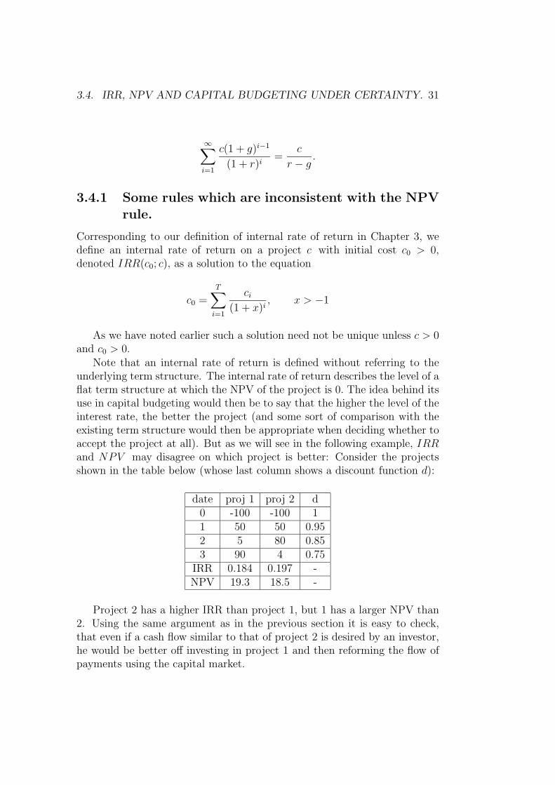
Note that an internal rate of return is defined without referring to theunderlying term structure. The internal rate of return describes the level of aflat term structure at which the NPV of the project is 0. The idea behind itsuse in capital budgeting would then be to say that the higher the level of theinterest rate, the better the project (and some sort of comparison with theexisting term structure would then be appropriate when deciding whether toaccept the project at all). But as we will see in the following example, IRRand NPV may disagree on which project is better: Consider the projectsshown in the table below (whose last column shows a discount function d):
date proj 1 proj 2 d0 -100 -100 11 50 50 0.952 5 80 0.853 90 4 0.75
IRR 0.184 0.197 -NPV 19.3 18.5 -
Project 2 has a higher IRR than project 1, but 1 has a larger NPV than2. Using the same argument as in the previous section it is easy to check,that even if a cash flow similar to that of project 2 is desired by an investor,he would be better off investing in project 1 and then reforming the flow ofpayments using the capital market.
32 CHAPTER 3. PAYMENT STREAMS UNDER CERTAINTY
Another problem with trying to use IRR as a decision variable arises whenthe IRR is not uniquely defined - something which typically happens whenthe cash flows exhibit sign changes. Which IRR should we then choose?
One might also contemplate using the payback method and count thenumber of years it takes to recover the initial cash outlay - possibly afterdiscounting appropriately the future cash flows. Project 2 in the table hasa payback of 2 years whereas project 1 has a payback of three years. Theexample above therefore also shows that choosing projects with the shortestpayback time may be inconsistent with the NPV method.
3.4.2 Several projects.
Consider someone with c0 > 0 available at date 0 who wishes to allocatethis capital over the T + 1 dates, and who considers a project c with initialcost c0. We have seen that precisely when NPV (c0; c) > 0 this person willbe able to obtain better cash flows by adopting c and trading in the capitalmarket than by trading in the capital market alone.
When there are several projects available the situation really does notchange much: Think of the i′th project (pi0, p) as an element of a set Pi ⊂RT+1. Assume that 0 ∈ Pi all i representing the choice of not starting the
i’th project. For a non-scalable project this set will consist of one point inaddition to 0.
Given a collection of projects represented by (Pi)i∈I . Situations wherethere is a limited amount of money to invest at the beginning (and borrow-ing is not permitted), where projects are mutually exclusive etc. may thenbe described abstractly by the requirement that the collection of selectedprojects (pi0, p
i)i∈I are chosen from a feasible subset P of the Cartesian prod-uct ×i∈IPi. The NPV of the chosen collection of projects is then just the sumof the NPVs of the individual projects and this in turn may be written asthe NPV of the sum of the projects:
∑i∈I
NPV (pi0; pi) = NPV
(∑i∈I
(pi0, pi)
).
Hence we may think of the chosen collection of projects as producing oneproject and we can use the result of the previous section to note that clearlyan investor should choose a project giving the highest NPV. Rather thanelaborating on this point, we consider an example.
Example 7 Consider the following example from Copeland and Weston (1988):
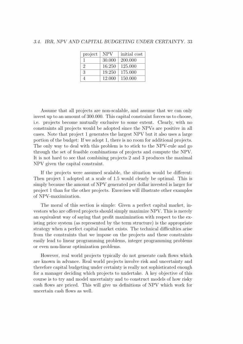
3.4. IRR, NPV AND CAPITAL BUDGETING UNDER CERTAINTY. 33
project NPV initial cost1 30.000 200.0002 16.250 125.0003 19.250 175.0004 12.000 150.000
Assume that all projects are non-scalable, and assume that we can onlyinvest up to an amount of 300.000. This capital constraint forces us to choose,i.e. projects become mutually exclusive to some extent. Clearly, with noconstraints all projects would be adopted since the NPVs are positive in allcases. Note that project 1 generates the largest NPV but it also uses a largeportion of the budget: If we adopt 1, there is no room for additional projects.The only way to deal with this problem is to stick to the NPV-rule and gothrough the set of feasible combinations of projects and compute the NPV.It is not hard to see that combining projects 2 and 3 produces the maximalNPV given the capital constraint.
If the projects were assumed scalable, the situation would be different:Then project 1 adopted at a scale of 1.5 would clearly be optimal. This issimply because the amount of NPV generated per dollar invested is larger forproject 1 than for the other projects. Exercises will illustrate other examplesof NPV-maximization.
The moral of this section is simple: Given a perfect capital market, in-vestors who are offered projects should simply maximize NPV. This is merelyan equivalent way of saying that profit maximization with respect to the ex-isting price system (as represented by the term structure) is the appropriatestrategy when a perfect capital market exists. The technical difficulties arisefrom the constraints that we impose on the projects and these constraintseasily lead to linear programming problems, integer programming problemsor even non-linear optimization problems.
However, real world projects typically do not generate cash flows whichare known in advance. Real world projects involve risk and uncertainty andtherefore capital budgeting under certainty is really not sophisticated enoughfor a manager deciding which projects to undertake. A key objective of thiscourse is to try and model uncertainty and to construct models of how riskycash flows are priced. This will give us definitions of NPV which work foruncertain cash flows as well.
34 CHAPTER 3. PAYMENT STREAMS UNDER CERTAINTY
3.5 Duration, convexity and immunization.
3.5.1 Duration with a flat term structure.
In this chapter we introduce the notions of duration and convexity which areoften used in practical bond risk management and asset/liability manage-ment. It is worth stressing that when we introduce dynamic models of theterm structure of interest rates in a world with uncertainty, we obtain muchmore sophisticated methods for measuring and controlling interest rate riskthan the ones presented in this section.
Consider a financial market which is arbitrage-free and complete andwhere the discount function d = (d1, . . . dT ) satisfies
di =1
(1 + r)ifor i = 1, . . . , T.
This corresponds to the assumption of a flat term structure. We stress thatthis assumption is rarely satisfied in practice but we will see how to relaxthis assumption.
What we are about to investigate are changes in present values as afunction of changes in r. This makes perfect sense even in a world of certainty,but sometimes we will speak freely of ’interest changes’ occurring even thoughstrictly speaking, we still do not have uncertainty in our model.
With a flat term structure, the present value of a payment stream c =(c1, . . . , cT ) is given by
PV (c; r) =T∑t=1
ct(1 + r)t
We have now included the dependence on r explicitly in our notation sincewhat we are about to model are essentially derivatives of PV (c; r) with re-spect to r.
Let c be a non-negative payment stream.
Definition 16 The duration D(c; r) of c is given by
D(c; r) =
(− ∂
∂rPV (c; r)
)1 + r
PV (c; r)(3.3)
=1
PV (c; r)
T∑t=1
tct
(1 + r)t
3.5. DURATION, CONVEXITY AND IMMUNIZATION. 35
This duration is called the Macaulay duration and is the “classical” one(many more advanced durations have been proposed in the literature). Ratherthat saying it is based on a flat term structure, we could refer to it as beingbased on the yield of the bond (or portfolio). Note that defining
wt =ct
(1 + r)t1
PV (c; r)(3.4)
we have∑T
t=1 wt = 1, hence
D(c; r) =T∑t=1
t wt.
Definition 17 The convexity of c is given by
K(c; r) =T∑t=1
t2 wt. (3.5)
where wt is given by (3.4).
Let us try to interpret D and K by computing the first and second deriva-tives3 of PV (c; r) with respect to r.
PV ′(c; r) = −T∑t=1
t ct1
(1 + r)t+1
= − 1
1 + r
T∑t=1
t ct1
(1 + r)t
PV ′′(c; r) =T∑t=1
t (t+ 1)ct
(1 + r)t+2
=1
(1 + r)2
[T∑t=1
t2ct1
(1 + r)t+
T∑t=1
tct1
(1 + r)t
]
Now consider the relative change in PV (c; r) when r changes to r + ∆r, i.e.
PV (c; r + ∆r)− PV (c; r)
PV (c; r)
3From now on we write PV ′(c; r) and PV ′′(c; r) instead of ∂∂rPV (c; r) resp. ∂2
∂r2PV (c; r)
36 CHAPTER 3. PAYMENT STREAMS UNDER CERTAINTY
By considering a second order Taylor expansion of the numerator, we obtain
PV (c; r + ∆r)− PV (c; r)
PV (c; r)≈
PV ′(c; r)∆r + 12PV ′′(c; r)(∆r)2
PV (c; r)
= −D ∆r
(1 + r)+
1
2(K +D)
(∆r
1 + r
)2
Hence D and K can be used to approximate the relative change inPV (c; r) as a function of the relative change in r (or more precisely, rela-
tive changes in 1 + r, since ∆(1+r)1+r
= ∆r1+r
).
Sometimes one finds the expression modified duration defined by
MD(c; r) =D
1 + r
and using this in a first order approximation, we get the relative change inPV (c; r) expressed by −MD(c; r)∆r, which is a function of ∆r itself. Theinterpretation of D as a price elasticity gives us no reasonable explanation ofthe word ’duration’, which certainly leads one to think of quantity measuredin units of time. If we use the definition of wt we have the following simpleexpression for the duration:
D(c; r) =T∑t=1
t wt.
Notice that wt expresses the present value of ct divided by the total presentvalue, i.e. wt expresses the weight by which ct is contributing to the totalpresent value. Since
∑Tt=1 wt = 1 we see that D(c; r) may be interpreted as
a ’mean waiting time’. The payment which occurs at time t is weighted bywt.
Example 8 For the government bullet bond in Example 5 the present valueof the payment stream is 106.75 and therefore the duration is∑4
k=1 tkck(1 + y)−tk
PV=
464.06
106.75= 4.35
while the convexity is∑4k=1 t
2kck(1 + y)−tk
PV=
2172.753
106.75= 20.35,
3.5. DURATION, CONVEXITY AND IMMUNIZATION. 37
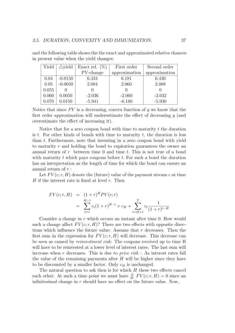
and the following table shows the the exact and approximated relative chancesin present value when the yield changes:
Yield 4yield Exact rel. (%) First order Second orderPV-change approximation approximation
0.04 -0.0150 6.434 6.181 6.4300.05 -0.0050 2.084 2.060 2.0880.055 0 0 0 00.060 0.0050 -2.036 -2.060 -2.0320.070 0.0150 -5.941 -6.180 -5.930
Notice that since PV is a decreasing, convex function of y we know that thefirst order approximation will underestimate the effect of decreasing y (andoverestimate the effect of increasing it).
Notice that for a zero coupon bond with time to maturity t the durationis t. For other kinds of bonds with time to maturity t, the duration is lessthan t. Furthermore, note that investing in a zero coupon bond with yieldto maturity r and holding the bond to expiration guarantees the owner anannual return of r between time 0 and time t. This is not true of a bondwith maturity t which pays coupons before t. For such a bond the durationhas an interpretation as the length of time for which the bond can ensure anannual return of r :
Let FV (c; r,H) denote the (future) value of the payment stream c at timeH if the interest rate is fixed at level r. Then
FV (c; r,H) = (1 + r)HPV (c; r)
=H−1∑t=1
ct(1 + r)H−t + cH +T∑
t=H+1
ct1
(1 + r)t−H
Consider a change in r which occurs an instant after time 0. How wouldsuch a change affect FV (c; r,H)? There are two effects with opposite direc-tions which influence the future value: Assume that r decreases. Then thefirst sum in the expression for FV (c; r,H) will decrease. This decrease canbe seen as caused by reinvestment risk: The coupons received up to time Hwill have to be reinvested at a lower level of interest rates. The last sum willincrease when r decreases. This is due to price risk : As interest rates fallthe value of the remaining payments after H will be higher since they haveto be discounted by a smaller factor. Only cH is unchanged.
The natural question to ask then is for which H these two effects canceleach other. At such a time point we must have ∂
∂rFV (c; r,H) = 0 since an
infinitesimal change in r should have no effect on the future value. Now,
38 CHAPTER 3. PAYMENT STREAMS UNDER CERTAINTY
∂
∂rFV (c; r,H) =
∂
∂r
[(1 + r)HPV (c; r)
]= H(1 + r)H−1PV (c; r) + (1 + r)HPV ′(c; r)
Setting this expression equal to 0 gives us
H =−PV ′(c; r)PV (c; r)
(1 + r)
i.e. H = D(c; r)
Furthermore, at H = D(c; r), we have ∂2
∂r2FV (c; r,H) > 0. This you can
check by computing ∂2
∂r2
((1 + r)HPV (c; r)
),reexpressing in terms D and K,
and using the fact that K > D2. Hence, at H = D(c; r), FV (c; r,H) will havea minimum in r. We say that FV (c; r,H) is immunized towards changes in r,but we have to interpret this expression with caution: The only way a bondreally can be immunized towards changes in the interest rate r between time0 and the investment horizon t is by buying zero coupon bonds with maturityt. Whenever we buy a coupon bond at time 0 with duration t, then to a firstorder approximation, an interest change immediately after time 0, will leavethe future value at time t unchanged. However, as date 1 is reached (say)it will not be the case that the duration of the coupon bond has decreasedto t − 1. As time passes, it is generally necessary to adjust bond portfoliosto maintain a fixed investment horizon, even if r is unchanged. This is trueeven in the case of certainty.
Later when we introduce dynamic hedging strategies we will see how aportfolio of bonds can be dynamically managed so as to truly immunize thereturn.
3.5.2 Relaxing the assumption of a flat term structure.
What we have considered above were parallel changes in a flat term structure.Since we rarely observe this in practice, it is natural to try and generalizethe analysis to different shapes of the term structure. Consider a family ofstructures given by a function r of two variables, t and x. Holding x fixedgives a term structure r(·, x).
For example, given a current term structure (y1, . . . , yT ) we could haver(t, x) = yt + x in which case changes in x correspond to additive changesin the current term structure (the one corresponding to x = 0). Or we couldhave 1 + r(t, x) = (1 + yt)x, in which case changes in x would produce multi-plicative changes in the current (obtained by letting x = 1) term structure.
3.5. DURATION, CONVEXITY AND IMMUNIZATION. 39
Now let us compute changes in present values as x changes:
∂PV
∂x= −
T∑t=1
tct1
(1 + r(t, x))t+1
∂r(t, x)
∂x
which gives us
∂PV
∂x
1
PV= −
T∑t=1
twt1 + r(t, x)
∂r(t, x)
∂x
where
wt =ct
(1 + r(t, x))t1
PV
We want to try and generalize the ’investment horizon’ interpretation ofduration, and hence calculate the future value of the payment stream attime H and differentiate with respect to x. Assume that the current termstructure is r(·, x0).
FV (c; r(H, x0), H) = (1 + r(H, x0))HPV (c; r(t, x0))
Differentiating
∂
∂xFV (c; r(H, x), H) = (1 + r(H, x))H
∂PV
∂x
+H(1 + r(H, x))H−1∂r(H, x)
∂xPV (c; r(t, x))
Evaluate this derivative at x = x0 and set it equal to 0 :
∂PV
∂x
∣∣∣∣x=x0
1
PV= −H ∂r(H, x)
∂x
∣∣∣∣x=x0
(1 + r(H, x0))−1
and hence we could define the duration corresponding to the given parametriza-tion as the value D for which
∂PV
∂x
∣∣∣∣x=x0
1
PV= −D ∂r(D, x)
∂x
∣∣∣∣x=x0
(1 + r(D, x0))−1.
The additive case would correspond to
∂r(D, x)
∂x
∣∣∣∣x=0
= 1,
40 CHAPTER 3. PAYMENT STREAMS UNDER CERTAINTY
and the multiplicative case to
∂r(D, x)
∂x
∣∣∣∣x=1
= 1 + yD.
Note that the multiplicative case gives us the duration measure (called theFisher-Weil duration)
Dmult = −∂PV∂x
1
PV=
T∑t=1
twt
which is just like the original measure although the weights of course reflectthe structure y(0, t).
Example 9 Consider again the small bond market from Example 4. Wehave already found the zero-coupon yields in the market, and find that theFisher-Weil duration of the 4 yr serial bond is
1
102.38
(32
1.0500+
2 ∗ 30.25
1.05502+
3 ∗ 28.5
1.06003+
4 ∗ 26.75
1.06504
)= 2.342,
and the following table gives the yields, Macaulay durations based on yieldsand Fisher-Weil durations for all the coupon bonds:
Bond Yield ( ) M-duration FW-duration1 yr bullet 5 1 12 yr bullet 5.49 1.952 1.952
3 yr annuity 5.65 1.963 1.9584 yr serial 5.93 2.354 2.342
3.5.3 An example
We finish this chapter with an example (with something usually referred toas a barbell strategy) which is intended to cause some concern. Some of theclaims are for you to check!
A financial institution issues 100 million $ worth of 10 year bullet bondswith time to maturity 10 years and a coupon rate of 7 percent. Assume thatthe term structure is flat at r = 7 percent. The revenue (of 100 million $) isused to purchase 10-and 20 year annuities also with coupon rates of 7%. Thenumbers of the 10 and 20 year annuities purchased are chosen in such a waythat the duration of the issued bullet bond matches that of the portfolio ofannuities. Now there are three facts you need to know at this stage. Letting
3.5. DURATION, CONVEXITY AND IMMUNIZATION. 41
T denote time to maturity, r the level of the term structure and γ the couponrate, we have that the duration of an annuity is given by
Dann =1 + r
r− T
(1 + r)T − 1.
Note that since payments on an annuity are equal in all periods we need notknow the size of the payments to calculate the duration.
The duration of a bullet bond is
Dbullet =1 + r
r− 1 + r − T (r −R)
R ((1 + r)T − 1) + r
which of course simplifies when r = R.The third fact you need to check is that if a portfolio consists of two
securities whose values are P1 and P2 respectively, then the duration of theportfolio P1 + P2 is given as
D(P1 + P2 ) =P1
P1 + P2
D(P1) +P2
P1 + P2
D(P2).
Using these three facts you will note that a portfolio consisting of 23.77million dollars worth of the 10-year annuity and 76.23 million dollars worth ofthe 20-year annuity will produce a portfolio whose duration exactly matchesthat of the issued bullet bond. By construction the present value of the twoannuities equals that of the bullet bond. The present value of the wholetransaction in other words is 0 at an interest level of 7 percent. However,for all other levels of the interest rate, the present value is strictly positive!In other words, any change away from 7 percent will produce a profit to thefinancial institution. We will have more to say about this phenomenon inthe exercises and we will return to it when discussing the term structure ofinterest rates in models with uncertainty. As you will see then, the reasonthat we can construct the example above is that we have set up an economyin which there are arbitrage opportunities.

42 CHAPTER 3. PAYMENT STREAMS UNDER CERTAINTY
Chapter 4
Arbitrage pricing in aone-period model
One of the biggest success stories of financial economics is the Black-Scholesmodel of option pricing. But even though the formula itself is easy to use,a rigorous presentation of how it comes about requires some fairly sophis-ticated mathematics. Fortunately, the so-called binomial model of optionpricing offers a much simpler framework and gives almost the same level ofunderstanding of the way option pricing works. Furthermore, the binomialmodel turns out to be very easy to generalize (to so-called multinomial mod-els) and more importantly to use for pricing other derivative securities (i.e.different contract types or different underlying securities) where an extensionof the Black-Scholes framework would often turn out to be difficult. The flex-ibility of binomial models is the main reason why these models are used dailyin trading all over the world.
Binomial models are often presented separately for each application. Forexample, one often sees the ”classical” binomial model for pricing options onstocks presented separately from binomial term structure models and pricingof bond options etc.
The aim of this chapter is to present the underlying theory at a levelof abstraction which is high enough to understand all binomial/multinomialapproaches to the pricing of derivative securities as special cases of one model.
Apart from the obvious savings in allocation of brain RAM that this pro-vides, it is also the goal to provide the reader with a language and frameworkwhich will make the transition to continuous-time models in future coursesmuch easier.
43
44 CHAPTER 4. ARBITRAGE PRICING IN A ONE-PERIOD MODEL
4.1 An appetizer.
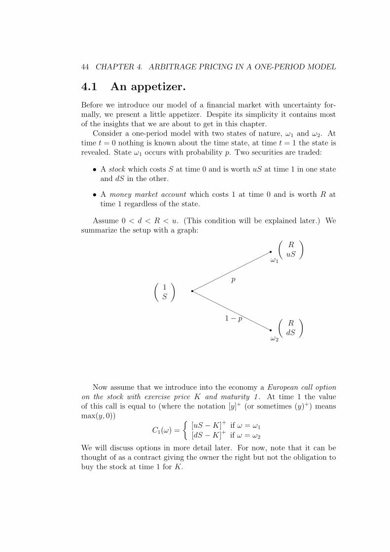
Before we introduce our model of a financial market with uncertainty for-mally, we present a little appetizer. Despite its simplicity it contains mostof the insights that we are about to get in this chapter.
Consider a one-period model with two states of nature, ω1 and ω2. Attime t = 0 nothing is known about the time state, at time t = 1 the state isrevealed. State ω1 occurs with probability p. Two securities are traded:
• A stock which costs S at time 0 and is worth uS at time 1 in one stateand dS in the other.
• A money market account which costs 1 at time 0 and is worth R attime 1 regardless of the state.
Assume 0 < d < R < u. (This condition will be explained later.) Wesummarize the setup with a graph:
r
HHHHHHHHH
HHHr
r(
1S
)
(RuS
)ω1
(RdS
)ω2
p
1− p
Now assume that we introduce into the economy a European call optionon the stock with exercise price K and maturity 1 . At time 1 the valueof this call is equal to (where the notation [y]+ (or sometimes (y)+) meansmax(y, 0))
C1(ω) =
[uS −K]+ if ω = ω1
[dS −K]+ if ω = ω2
We will discuss options in more detail later. For now, note that it can bethought of as a contract giving the owner the right but not the obligation tobuy the stock at time 1 for K.

4.1. AN APPETIZER. 45
To simplify notation, let Cu = C1(ω1) and Cd = C1(ω2). The question is:What should the price of this call option be at time 0? A simple portfolioargument will give the answer: Let us try to form a portfolio at time 0 usingonly the stock and the money market account which gives the same payoffas the call at time 1 regardless of which state occurs. Let (a, b) denote,respectively, the number of stocks and units of the money market accountheld at time 0. If the payoff at time 1 has to match that of the call, we musthave
a(uS) + bR = Cu
a(dS) + bR = Cd
Subtracting the second equation from the first we get
a(u− d)S = Cu − Cd
i.e.
a =Cu − CdS(u− d)
and algebra gives us
b =1
R
uCd − dCu(u− d)
where we have used our assumption that u > d. The cost of forming theportfolio (a, b) at time 0 is
(Cu − Cd)S (u− d)
S +1
R
uCd − dCu(u− d)
· 1
=R (Cu − Cd)R (u− d)
+1
R
uCd − dCu(u− d)
=1
R
[R− du− d
Cu +u−Ru− d
Cd
].
We will formulate below exactly how to define the notion of no arbitragewhen there is uncertainty, but it should be clear that the argument we havejust given shows why the call option must have the price
C0 =1
R
[R− du− d
Cu +u−Ru− d
Cd
]Rewriting this expression we get
C0 =
(R− du− d
)CuR
+
(u−Ru− d
)CdR
46 CHAPTER 4. ARBITRAGE PRICING IN A ONE-PERIOD MODEL
and if we let
q =R− du− d
we get
C0 = qCuR
+ (1− q)CdR.
If the price were lower, one could buy the call and sell the portfolio (a, b),receive cash now as a consequence and have no future obligations except toexercise the call if necessary.
Some interesting features of this example will be much clearer as we goalong:
• The probability p plays no role in the expression for C0.
• A new set of probabilities
q =R− du− d
and 1− q =u−Ru− d
emerges (this time we also use that d < R < u) and with this set ofprobabilities we may write the value of the call as
C0 = Eq
[C1(ω)
R
]i.e. an expected value using q of the discounted time 1 value of thecall.
• If we compute the expected value using q of the discounted time 1 stockprice we find
Eq
[S(ω)
R
]=
(R− du− d
)1
R(uS) +
(u−Ru− d
)1
R(dS) = S
The method of pricing the call really did not use the fact that Cu and Cdwere call-values. Any security with a time 1 value depending on ω1 and ω2
could have been priced.
4.2 The single period model
The mathematics used when considering a one-period financial market withuncertainty is exactly the same as that used to describe the bond market ina multiperiod model with certainty: Just replace dates by states.
4.2. THE SINGLE PERIOD MODEL 47
Given two time points t = 0 and t = 1 and a finite state space
Ω = ω1, . . . , ωS .
Whenever we have a probability measure P (or Q) we write pi (or qi) insteadof P (ωi) (or Q (ωi)).
A security price system is a vector π ∈ RN and an N×S matrix D wherewe interpret the i’th row (di1, . . . , diS) of D as the payoff at time 1 of thei’th security in states 1, . . . , S, respectively. The price at time 0 of the i’thsecurity is πi. A portfolio is a vector θ ∈ RN whose coordinates represent thenumber of securities bought at time 0. The price of the portfolio θ boughtat time 0 is π · θ.
Definition 18 An arbitrage in the security price system (π,D) is a portfolioθ which satisfies either
π · θ ≤ 0 ∈ R and D>θ > 0 ∈ RS
orπ · θ < 0 ∈ R and D>θ ≥ 0 ∈ R S
A security price system (π,D) for which no arbitrage exists is called arbitrage-free.
Remark 1 Our conventions when using inequalities on a vector in Rk arethe same as described in Chapter 3.
When a market is arbitrage-free we want a vector of prices of ’elementarysecurities’ - just as we had a vector of discount factors in Chapter 3.
Definition 19 ψ ∈ RS++ (i.e. ψ 0) is said to be a state-price vector forthe system (π,D) if it satisfies
π = Dψ
Clearly, we have already proved the following in Chapter 3:
Proposition 6 A security price system is arbitrage-free if and only if thereexists a state-price vector.
Unlike the model we considered in Chapter 3, the security which pays 1in every state plays a special role here. If it exists, it allows us to speak ofan ’interest rate’:
48 CHAPTER 4. ARBITRAGE PRICING IN A ONE-PERIOD MODEL
Definition 20 The system (π,D) contains a riskless asset if there exists alinear combination of the rows of D which gives us (1, . . . , 1) ∈ RS.
In an arbitrage-free system the price of the riskless asset d0 is called thediscount factor and R0 ≡ 1
d0is the return on the riskless asset. Note that
when a riskless asset exists, and the price of obtaining it is d0, we have
d0 = θ>0 π = θ>0 Dψ = ψ1 + · · ·+ ψS
where θ0 is the portfolio that constructs the riskless asset.Now define
qi =ψid0
, i = 1, . . . , S
Clearly, qi > 0 and∑S
i=1 qi = 1, so we may interpret the qi’s as probabilities.We may now rewrite the identity (assuming no arbitrage) π = Dψ as follows:
π = d0Dq =1
R0
Dq, where q = (q1, . . . , qS)>
If we read this coordinate by coordinate it says that
πi =1
R0
(q1di1 + . . .+ qSdiS)
which is the discounted expected value using q of the i’th security’s payoffat time 1. Note that since R0 is a constant we may as well say ”expecteddiscounted . . .”.
We assume throughout the rest of this section that a riskless asset exists.
Definition 21 A security c = (c1, . . . , cS) is redundant given the securityprice system (π,D) if there exists a portfolio θc such that Dtθc = c.
Proposition 7 Let an arbitrage-free system (π,D) and a redundant security
c by given. The augmented system(π, D
)obtained by adding πc to the vector
π and c ∈ RS as a row of D is arbitrage-free if and only if
πc =1
R0
(q1c1 + . . .+ qScS) ≡ ψ1c1 + . . .+ ψScS.
Proof. Assume πc < ψ1c1 + . . . + ψScS. Buy the security c and sell theportfolio θc. The price of θc is by assumption higher than πc, so we receivea positive cash-flow now. The cash-flow at time 1 is 0. Hence there is anarbitrage opportunity. If πc > ψ1c1 + . . .+ ψScS reverse the strategy.
4.2. THE SINGLE PERIOD MODEL 49
Definition 22 The market is complete if for every y ∈ RS there exists aθ ∈ RN such that
D>θ = y
i.e. if the rows of D (the columns of D>) span RS.
Proposition 8 If the market is complete and arbitrage-free, there exists pre-cisely one state-price vector ψ.
The proof is exactly as in Chapter 3 and we are ready to do contingentclaims pricing! Here is how it is done in a one-period model: Construct aset of securities (the D-matrix,) and a set of prices. Make sure that (π,D)is arbitrage-free. Make sure that either
(a) the model is complete, i.e. there are as many linearly independentsecurities as there are states
or(b) the contingent claim we wish to price is redundant given (π,D).Clearly, (a) implies (b) but not vice versa. (a) is almost always what is
done in practice. Given a ”contingent claim” c = (c1, . . . , cS). Now computethe price of the contingent claim as
π (c) =1
R0
Eq (c) ≡ 1
R0
S∑i=1
qici
where qi = ψid0≡ R0ψi. The portfolio generating the claim is the solution to
D>θc = c, and since we can always in a complete model reduce the matrixto an S × S invertible matrix without changing the model this can be doneby matrix inversion.
Let us return to our example in the beginning of this chapter: The securityprice system is (
1S
),
(R RuS dS
).
For this to be arbitrage-free, proposition (6) tells us that there must be asolution (ψ1, ψ2) with ψ1 > 0 and ψ2 > 0 to the equation(
1S
)=
(R RuS dS
)(ψ1
ψ2
).
u 6= d ensures that the matrix
(R RuS dS
)has full rank. u > d can be
assumed without loss of generality. We find
ψ1 =R− d
R (u− d)
50 CHAPTER 4. ARBITRAGE PRICING IN A ONE-PERIOD MODEL
ψ2 =u−R
R (u− d)
and note that the solution is strictly positive precisely when u > R > d(given our assumption that u > d > 0).
Clearly the riskfree asset has a return of R, and
q1 = Rψ1 =R− du− d
q2 = Rψ2 =u−Ru− d
are the probabilities defining the measure q which can be used for pricing.Note that the market is complete, and this explains why we could use theprocedure in the previous example to say what the correct price at time 0 ofany claim (c1, c2) should be.
4.3 The economic intuition
At first, it may seem surprising that the ’objective’ probability p does notenter into the expression for the option price. Even if the the probability is0.99 making the probability of the option paying out a positive amount verylarge, it does not alter the option’s price at time 0. Looking at this problemfrom a mathematical viewpoint, one can just say that this is a consequence ofthe linear algebra of the problem: The cost of forming a replicating strategydoes not depend on the probability measure and therefore it does not enterinto the contract. But this argument will not (and should not) convince aperson who is worried by the economic interpretation of a model. Addressingthe problem from a purely mathematical angle leaves some very importanteconomic intuition behind. We will try in this section to get the economicintuition behind this ’invariance’ to the choice of p straight. This will providean opportunity to outline how the financial markets studied in this course fitin with a broader microeconomic analysis.
Before the more formal approach, here is the story in words: If we argue(erroneously) that changing p ought to change the option’s price at time 0,the same argument should also lead to a suggested change in S0. But theexperiment involving a change in p is an experiment which holds S0 fixed.The given price of the stock is supposed to represent a ’sensible’ model of themarket. If we change p without changing S0 we are implicitly changing ourdescription of the underlying economy. An economy in which the probabilityof an up jump p is increased to 0.99 while the initial stock price remainsfixed must be a description of an economy in which payoff in the upstate has
4.3. THE ECONOMIC INTUITION 51
lost value relative to a payoff in the downstate. These two opposite effectsprecisely offset each other when pricing the option.
The economic model we have in mind when studying the financial marketis one in which utility is a function of wealth in each state and wealth ismeasured by a scalar (kroner, dollars, . . .). Think of the financial marketas a way of transferring money between different time periods and differentstates. A real economy would have a (spot) market for real goods also (food,houses, TV-sets, . . .) and perhaps agents would have known endowments ofreal goods in each state at each time. If the spot prices of real goods whichare realized in each state at each future point in time are known at time 0,then we may as well express the initial endowment in terms of wealth in eachstate. Similarly, the optimal consumption plan is associated with a precisetransfer of wealth between states which allows one to realize the consumptionplan. So even if utility is typically a function of the real goods (most peoplelike money because of the things it allows them to buy), we can formulatethe utility as a function of the wealth available in each state.
Consider1 an agent who has an endowment e = (e1, . . . , eS) ∈ RS+. Thisvector represents the random wealth that the agent will have at time 1. Theagent has a utility function U : RS+ → R which we assume to be concave,differentiable and strictly increasing in each coordinate. Given a financialmarket represented by the pair (π,D), the agent’s problem is
maxθU(e + D>θ) (4.1)
s.t. π>θ ≤ 0.
If we assume that there exists a security with a non-negative payoff whichis strictly positive in at least one state, then because the utility functionis increasing we can replace the inequality in the constraint by an equality.And then the interpretation is simply that the agent sells endowment in somestates to obtain more in other states. But no cash changes hands at time 0.Note that while utility is defined over all (non-negative) consumption vectors,it is the rank of D which decides in which directions the consumer can moveaway from the initial endowment.
Now make sure that you can prove the following
Proposition 9 If there exists a portfolio θ with D>θ > 0 then the agent canfind a solution to the maximization problem if and only if (π,D) is arbitrage-free.
1This closely follows Darrell Duffie: Dynamic Asset Pricing Theory. Princeton Univer-sity Press. 1996
52 CHAPTER 4. ARBITRAGE PRICING IN A ONE-PERIOD MODEL
The ’only if’ part of this statement shows how no arbitrage is a necessarycondition for existence of a solution to the agent’s problem and hence for theexistence of equilibrium for economies where agents have increasing utility(no continuity assumptions are needed here). The ’if’ part uses continuityand compactness (why?) to ensure existence of a maximum, but of course todiscuss equilibrium would require more agents and then we need some moreof our general equilibrium apparatus to prove existence.
The important insight is the following (see Proposition 1C in Duffie(1996)):
Proposition 10 Assume that there exists a portfolio θ with D>θ > 0. Ifthere exists a solution θ∗ to (4.1) and the associated optimal consumptionis given by c∗ := e + D>θ∗ >> 0, then the gradient ∇U(c∗) (thought ofas a column vector) is proportional to a state-price vector. The constant ofproportionality is positive.
Proof. Since c∗ is strictly positive, then for any portfolio θ there existssome k(θ) such that c∗ + αD>θ ≥ 0 for all α in [−k(θ), k(θ)]. Define
gθ : [−k(θ), k(θ)]→ R
asgθ(α) = U(c∗ + αD>θ)
Now consider a θ with π>θ = 0. Since c∗ is optimal, gθ must be maximizedat α = 0 and due to our differentiability assumptions we must have
g′θ(0) = (∇U(c∗))>D>θ = 0.
We can conclude that any θ with π>θ = 0 satisfies (∇U(c∗))>D>θ = 0. Trans-posing the last expression, we may also write θ>D∇U(c∗) = 0. In words, anyvector which is orthogonal to π is also orthogonal to D∇U(c∗). This meansthat µπ = D∇U(c∗) for some µ showing that ∇U(c∗) is proportional to astate-price vector. Choosing a θ+ with D>θ+ > 0 we know from no arbitragethat π>θ+ > 0 and from the assumption that the utility function is strictlyincreasing, we have ∇U(c∗)D>θ+ > 0. Hence µ must be positive.
To understand the implications of this result we turn to the special casewhere the utility function has an expected utility representation, i.e. wherewe have a set of probabilities (p1, . . . , pS) and a function u such that
U(c) =S∑i=1
piu(ci).
4.3. THE ECONOMIC INTUITION 53
In this special case we note that the coordinates of the state-price vectorsatisfy
ψi = λpiu′(c∗i ), i = 1, . . . , S. (4.2)
where λ is some constant of proportionality. Now we can state the economicintuition behind the option example as follows (and it is best to think ofa complete market to avoid ambiguities in the interpretation): Given thecomplete market (π,D) we can find a unique state price vector ψ. This stateprice vector does not depend on p. Thus if we change p and we are think-ing of some agent out there ’justifying’ our assumptions on prices of tradedsecurities, it must be the case that the agent has different marginal utili-ties associated with optimal consumption in each state. The difference mustoffset the change in p in such a way that (4.2) still holds. We can thinkof this change in marginal utility as happening in two ways: One way is tochange utility functions altogether. Then starting with the same endowmentthe new utility functions would offset the change in probabilities so that theequality still holds. Another way to think of state prices as being fixed withnew probabilities but utility functions unchanged, is to think of a differentvalue of the initial endowment. If the endowment is made very large in onestate and very small in the other, then this will offset the large change inprobabilities of the two states. The analysis of the single agent can be carriedover to an economy with many agents with suitable technical assumptions.Things become particularly easy when the equilibrium can be analyzed byconsidering the utility of a single, ’representative’ agent, whose endowmentis the sum of all the agents’ endowments. An equilibrium then occurs only ifthis representative investor has the initial endowment as the solution to theutility maximization problem and hence does not need to trade in the marketwith the given prices. In this case the aggregate endowment plays a crucialrole. Increasing the probability of a state while holding prices and the utilityfunction of the representative investor constant must imply that the aggre-gate endowment is different with more endowment (low marginal utility) inthe states with high probability and low endowment (high marginal utility)in the states with low probability. This intuition is very important when wediscuss the Capital Asset Pricing Model later in the course.
A market where we are able to separate out the financial decisions asabove is the one we will have in our mind throughout this course. But do keepin mind that this leaves out many interesting issues in the interaction betweenreal markets and financial markets. For example, it is easy to imagine that anincomplete financial market (i.e. one which does not allow any distributionof wealth across states and time periods) makes it impossible for agents torealize consumption plans that they would find optimal in a complete market.
54 CHAPTER 4. ARBITRAGE PRICING IN A ONE-PERIOD MODEL
This in turn may change equilibrium prices on real markets because it changesinvestment behavior. For example, returning to the house market, the factthat financial markets allows young agents to borrow against future income,makes it possible for more consumers to buy a house early in their lives. Ifall of a sudden we removed the possibility of borrowing we could imaginethat house prices would drop significantly, since the demand would suddenlydecrease.
Chapter 5
Arbitrage pricing in themulti-period model
5.1 An appetizer
It is fair to argue that to get realism in a model with finite state space weneed the number of states to be large. After all, why would the stock takeon only two possible values at the expiration date of the option? On theother hand, we know from the previous section that in a model with manystates we need many securities to have completeness, which (in arbitrage-freemodels) is a requirement for pricing every claim. And if we want to pricean option using only the underlying stock and a money market account, weonly have two securities to work with. Fortunately, there is a clever way outof this.
Assume that over a short time interval the stock can only move to twodifferent values and split up the time interval between 0 and T (the maturitydate of an option) into small intervals in which the stock can be traded.Then it turns out that we can have both completeness and therefore arbitragepricing even if the number of securities is much smaller than the number ofstates. Again, before we go into the mathematics, we give an example tohelp with the intuition.
Assume that Ω = ω1, ω2, ω3, ω4 and that there are three dates: t ∈0, 1, 2. We specify the behavior of the stock and the money market accountas follows: Assume that 0 < d < R < u and that S > 0. Consider thefollowing graph:
55
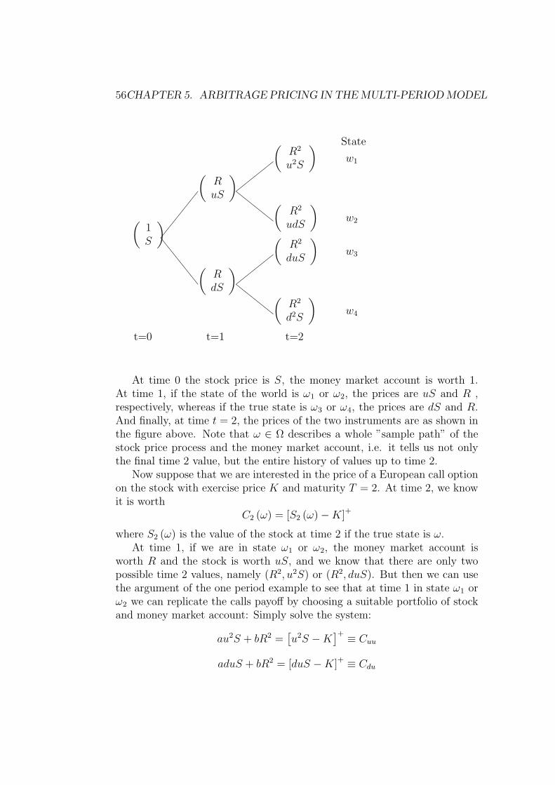
56CHAPTER 5. ARBITRAGE PRICING IN THE MULTI-PERIOD MODEL
(1S
)
\\\\\
(RuS
)
(RdS
)
####
cccc
(R2
u2S
)
(R2
udS
)
####
cccc
(R2
duS
)
(R2
d2S
)
w1
w2
w3
w4
State
t=0 t=1 t=2
At time 0 the stock price is S, the money market account is worth 1.At time 1, if the state of the world is ω1 or ω2, the prices are uS and R ,respectively, whereas if the true state is ω3 or ω4, the prices are dS and R.And finally, at time t = 2, the prices of the two instruments are as shown inthe figure above. Note that ω ∈ Ω describes a whole ”sample path” of thestock price process and the money market account, i.e. it tells us not onlythe final time 2 value, but the entire history of values up to time 2.
Now suppose that we are interested in the price of a European call optionon the stock with exercise price K and maturity T = 2. At time 2, we knowit is worth
C2 (ω) = [S2 (ω)−K]+
where S2 (ω) is the value of the stock at time 2 if the true state is ω.At time 1, if we are in state ω1 or ω2, the money market account is
worth R and the stock is worth uS, and we know that there are only twopossible time 2 values, namely (R2, u2S) or (R2, duS). But then we can usethe argument of the one period example to see that at time 1 in state ω1 orω2 we can replicate the calls payoff by choosing a suitable portfolio of stockand money market account: Simply solve the system:
au2S + bR2 =[u2S −K
]+ ≡ Cuu
aduS + bR2 = [duS −K]+ ≡ Cdu
5.1. AN APPETIZER 57
for (a, b) and compute the price of forming the portfolio at time 1. We find
a =Cuu − CduuS (u− d)
, b =uCdu − dCuu(u− d)R2
.
The price of this portfolio is
auS + bR =R
R
(Cuu − Cdu)(u− d)
+uCdu − dCuu
(u− d)R
=1
R
[(R− d)
(u− d)Cuu +
(u−R)
(u− d)Cud
]=: Cu
This is clearly what the call is worth at time t = 1 if we are in ω1
or ω2, i.e. if the stock is worth uS at time 1. Similarly, we may defineCud := [udS −K]+ (which is equal to Cdu) and Cdd = [d2S −K]
+. And now
we use the exact same argument to see that if we are in state ω3 or ω4, i.e.if the stock is worth dS at time 1, then at time 1 the call should be worthCd where
Cd :=1
R
[(R− d)
(u− d)Cud +
(u−R)
(u− d)Cdd
].
Now we know what the call is worth at time 1 depending on which statewe are in: If we are in a state where the stock is worth uS, the call is worthCu and if the stock is worth dS, the call is worth Cd.
Looking at time 0 now, we know that all we need at time 1 to be able to”create the call”, is to have Cu when the stock goes up to uS and Cd whenit goes down. But that we can accomplish again by using the one-periodexample: The cost of getting
(CuCd
)is
C0 :=1
R
[(R− d)
(u− d)Cu +
(u−R)
(u− d)Cd
].
If we let q = R−du−d and if we insert the expressions for Cu and Cd, noting
that Cud = Cdu, we find that
C0 =1
R2
[q2Cuu + 2q (1− q)Cud + (1− q)2 Cdd
]which the reader will recognize as a discounted expected value, just as in theone period example. (Note that the representation as an expected value doesnot hinge on Cud = Cdu.)
The important thing to understand in this example is the following: Start-ing out with the amount C0, an investor is able to form a portfolio in thestock and the money market account which produces the payoffs Cu or Cd
58CHAPTER 5. ARBITRAGE PRICING IN THE MULTI-PERIOD MODEL
at time 1 depending on where the stock goes. Now without any additionalcosts, the investor can rearrange his/her portfolio at time 1, such that attime 2, the payoff will match that of the option. Therefore, at time 0 theprice of the option must be C0.
This ”dynamic hedging” argument is the key to pricing derivative securi-ties in discrete-time, finite state space models. We now want to understandthe mathematics behind this example.
5.2 Price processes, trading and arbitrage
Given a probability space (Ω,F , P ) with Ω finite, let F := 2Ω (i.e. the set ofall subsets of Ω) and assume that P (ω) > 0 for all ω ∈ Ω. Also assume thatthere are T+1 dates, starting at date 0, ending at date T. To formalize howinformation is revealed through time, we introduce the notion of a filtration:
Definition 23 A filtration F = FtTt=0 is an increasing sequence of σ-algebras contained in F :F0 ⊆ F1 ⊆ . . . ⊆ FT .
We will always assume that F0 = ∅,Ω and FT = F . Since Ω is finite,it will be easy to think of the σ−algebras in terms of partitions:
Definition 24 A partition Pt of Ω is a collection of non-empty subsets ofΩ such that
•⋃
Pi∈PtPi = Ω
• Pi ∩ Pj = ∅ whenever i 6= j, Pi, Pj ∈ Pt.
Because Ω is finite, there is a one-to-one correspondence between parti-tions and σ−algebras: The elements of Pt corresponds to the atoms of Ft.
The concepts we have just defined are well illustrated in an event-tree:
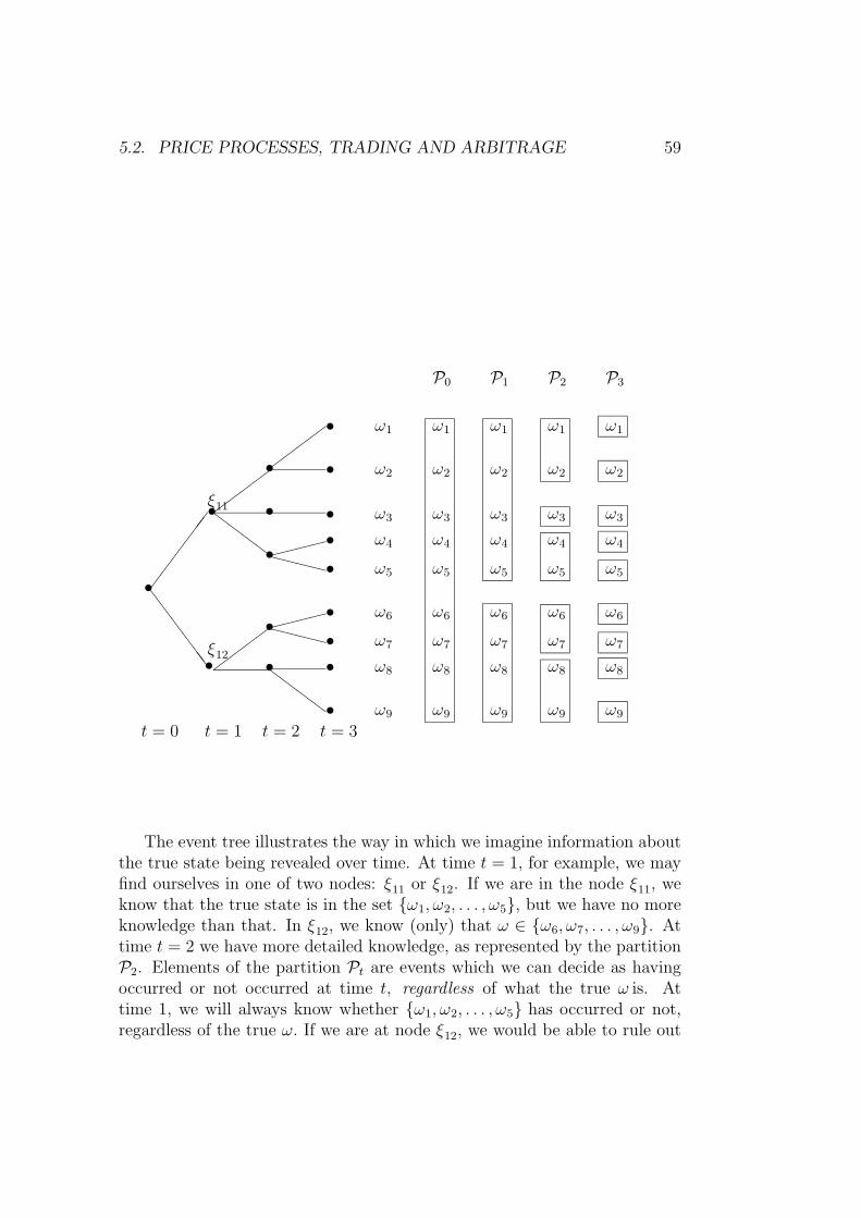
5.2. PRICE PROCESSES, TRADING AND ARBITRAGE 59
•
SSSSSS
•ξ11
ZZZZ
•ξ12
••
•
• •
•
XXXX
••
•
XXXX
••
•ZZZZ
•
•
P0 P1 P2 P3
ω1
ω2
ω3
ω4
ω5
ω6
ω7
ω8
ω9
ω1
ω2
ω3
ω4
ω5
ω6
ω7
ω8
ω9
ω1
ω2
ω3
ω4
ω5
ω6
ω7
ω8
ω9
ω1
ω2
ω3
ω4
ω5
ω6
ω7
ω8
ω9
ω1
ω2
ω3
ω4
ω5
ω6
ω7
ω8
ω9
t = 0 t = 1 t = 2 t = 3
The event tree illustrates the way in which we imagine information aboutthe true state being revealed over time. At time t = 1, for example, we mayfind ourselves in one of two nodes: ξ11 or ξ12. If we are in the node ξ11, weknow that the true state is in the set ω1, ω2, . . . , ω5, but we have no moreknowledge than that. In ξ12, we know (only) that ω ∈ ω6, ω7, . . . , ω9. Attime t = 2 we have more detailed knowledge, as represented by the partitionP2. Elements of the partition Pt are events which we can decide as havingoccurred or not occurred at time t, regardless of what the true ω is. Attime 1, we will always know whether ω1, ω2, . . . , ω5 has occurred or not,regardless of the true ω. If we are at node ξ12, we would be able to rule out
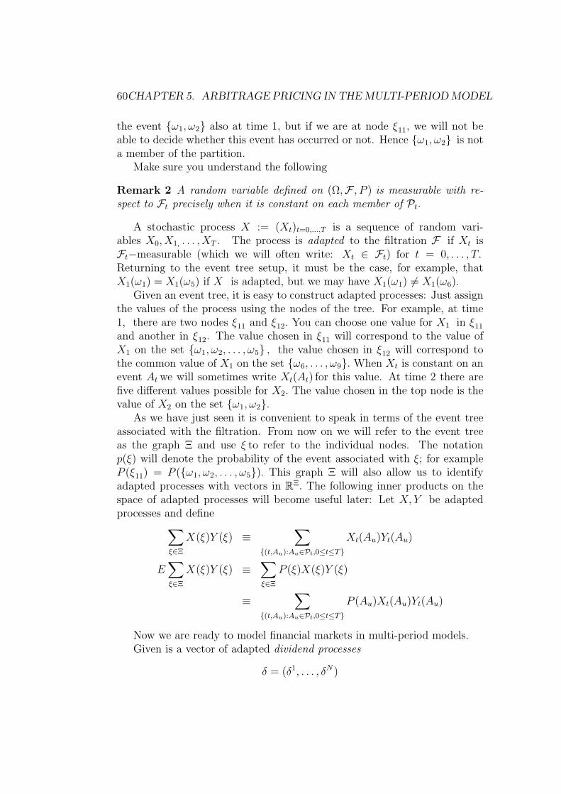
60CHAPTER 5. ARBITRAGE PRICING IN THE MULTI-PERIOD MODEL
the event ω1, ω2 also at time 1, but if we are at node ξ11, we will not beable to decide whether this event has occurred or not. Hence ω1, ω2 is nota member of the partition.
Make sure you understand the following
Remark 2 A random variable defined on (Ω,F , P ) is measurable with re-spect to Ft precisely when it is constant on each member of Pt.
A stochastic process X := (Xt)t=0,...,T is a sequence of random vari-ables X0, X1, . . . , XT . The process is adapted to the filtration F if Xt isFt−measurable (which we will often write: Xt ∈ Ft) for t = 0, . . . , T.Returning to the event tree setup, it must be the case, for example, thatX1(ω1) = X1(ω5) if X is adapted, but we may have X1(ω1) 6= X1(ω6).
Given an event tree, it is easy to construct adapted processes: Just assignthe values of the process using the nodes of the tree. For example, at time1, there are two nodes ξ11 and ξ12. You can choose one value for X1 in ξ11
and another in ξ12. The value chosen in ξ11 will correspond to the value ofX1 on the set ω1, ω2, . . . , ω5 , the value chosen in ξ12 will correspond tothe common value of X1 on the set ω6, . . . , ω9. When Xt is constant on anevent At we will sometimes write Xt(At) for this value. At time 2 there arefive different values possible for X2. The value chosen in the top node is thevalue of X2 on the set ω1, ω2.
As we have just seen it is convenient to speak in terms of the event treeassociated with the filtration. From now on we will refer to the event treeas the graph Ξ and use ξ to refer to the individual nodes. The notationp(ξ) will denote the probability of the event associated with ξ; for exampleP (ξ11) = P (ω1, ω2, . . . , ω5). This graph Ξ will also allow us to identifyadapted processes with vectors in RΞ. The following inner products on thespace of adapted processes will become useful later: Let X,Y be adaptedprocesses and define∑
ξ∈Ξ
X(ξ)Y (ξ) ≡∑
(t,Au):Au∈Pt,0≤t≤T
Xt(Au)Yt(Au)
E∑ξ∈Ξ
X(ξ)Y (ξ) ≡∑ξ∈Ξ
P (ξ)X(ξ)Y (ξ)
≡∑
(t,Au):Au∈Pt,0≤t≤T
P (Au)Xt(Au)Yt(Au)
Now we are ready to model financial markets in multi-period models.Given is a vector of adapted dividend processes
δ = (δ1, . . . , δN)
5.2. PRICE PROCESSES, TRADING AND ARBITRAGE 61
and a vector of adapted security price processes
S = (S1, . . . , SN).
The interpretation is as follows: Sit(ω) is the price of security i at time t if thestate is ω. Buying the i′th security at time t ensures the buyer (and obligatesthe seller to deliver) the remaining dividends δit+1, δ
it+2, . . . , δ
iT .
1 Hence thesecurity price process is to be interpreted as an ex-dividend price processand in particular we should think of ST as 0. In all models considered inthese notes we will also assume that there is a money market account whichprovides locally riskless borrowing and lending. This is modeled as follows:Given an adapted process - the spot rate process
ρ = (ρ0, ρ1, . . . , ρT−1).
To make the math work, all we need to assume about this process is that itis strictly greater than −1 at all times and in all states, but for modellingpurposes it is desirable to have it non-negative. Now we may define themoney market account as follows:
Definition 25 The money market account has the security price process
S0t = 1, t = 0, 1, . . . , T − 1
S0T = 0.
and the dividend process
δ0t (ω) = ρt−1(ω) for all ω and t = 1, . . . , T − 1,
δ0T (ω) = 1 + ρT−1(ω).
This means that if you buy one unit of the money market account at timet you will receive a dividend of ρt at time t+ 1. Since ρt is known already attime t, the dividend received on the money market account in the next periodt+ 1 is known at time t. Since the price is also known to be 1 you know thatplacing 1 in the money market account at time t and selling the asset at timet+ 1 will give you 1 +ρt.This is why we refer to this asset as a locally risklessasset.You may of course also choose to keep the money in the money marketaccount and receive the stream of dividends. Reinvesting the dividends in themoney market account will make this account grow according to the processR defined as
Rt = (1 + ρ0) · · · (1 + ρt−1).
1We will follow the tradition of probability theory and often suppress the ω in thenotation.
62CHAPTER 5. ARBITRAGE PRICING IN THE MULTI-PERIOD MODEL
We will need this process to discount cash flows between arbitrary periodsand therefore introduce the following notation:
Rs,t ≡ (1 + ρs) · · · (1 + ρt−1).
Definition 26 A trading strategy is an adapted process
φ = (φ0t , . . . , φ
Nt )t=0,...,T−1.
and the interpretation is that φit(ω) is the number of the i′th security held attime t if the state is ω. The requirement that the trading strategy is adaptedis very important. It represents the idea that the strategy should not be ableto see into the future. Returning again to the event tree, when standing innode ξ11, a trading strategy can base the number of securities on the factthat we are in ξ11 (and not in ξ12), but not on whether the true state is ω1
or ω2.The dividend stream generated by the trading strategy φ is denoted δφ
and it is defined as
δφ0 = −φ0 · S0
δφt = φt−1 · (St + δt)− φt · St for t = 1, . . . , T.
Definition 27 An arbitrage is a trading strategy for which δφt is a positiveprocess, i.e. always nonnegative and δφt (ω) > 0 for some t and ω. The modelis said to be arbitrage-free if it contains no arbitrage opportunities.
In words, there is arbitrage if we can adopt a trading strategy which atno point in time requires us to pay anything but which at some time in somestate gives us a strictly positive payout. Note that since we have included theinitial payout as part of the dividend stream generated by a trading strategy,we can capture the definition of arbitrage in this one statement. This onestatement captures arbitrage both in the sense of receiving money now withno future obligations and in the sense of paying nothing now but receivingsomething later.
Definition 28 A trading strategy φ is self-financing if it satisfies
φt−1 · (St + δt) = φt · St for t = 1, . . . , T.
The interpretation is as follows: Think of forming a portfolio φt−1 attime t − 1. Now as we reach time t, the value of this portfolio is equal toφt−1 · (St + δt), and for a self-financing trading strategy, this is precisely theamount of money which can be used in forming a new portfolio at time t.We will let Φ denote the set of self-financing trading strategies.
5.3. NO ARBITRAGE AND PRICE FUNCTIONALS 63
5.3 No arbitrage and price functionals
We have seen in the one period model that there is equivalence between theexistence of a state price vector and absence of arbitrage. In this section weshow the multi-period analogue of this theorem.
The goal of this section is to prove the existence of the multi-periodanalogue of state-price vectors in the one-period model. Let L denote the setof adapted processes on the given filtration.
Definition 29 A pricing functional F is a linear functional
F : L→R
which is strictly positive, i.e.
F (X) ≥ 0 for X ≥ 0
F (X) > 0 for X > 0.
Definition 30 A pricing functional F is consistent with security prices if
F (δφ) = 0 for all trading strategies φ.
Note that if there exists a consistent pricing functional we may arbitrarilyassume that the value of the process 1t=0 (i.e. the process which is 1 at time0 and 0 thereafter) is 1.
By Riesz’ representation theorem we can represent the functional F as
F (X) =∑ξ∈Ξ
X(ξ)f(ξ)
With the convention F (1t=0) = 1, we then note that if there exists a tradingstrategy φwhich is initiated at time 0 and which only pays a dividend of 1 inthe node ξ, then
φ0 · S0 = f(ξ).
Hence f(ξ) is the price at time 0 of having a payout of 1 in the node ξ.
Proposition 11 The model (δ, S) is arbitrage-free if and only if there existsa consistent pricing functional.
Proof. First, assume that there exists a consistent pricing functional F. Anydividend stream δφ generated by a trading strategy which is positive musthave F (δφ) > 0 but this contradicts consistency. Hence there is no arbitrage.The other direction requires more work:
64CHAPTER 5. ARBITRAGE PRICING IN THE MULTI-PERIOD MODEL
Define the sets
L1 =
X ∈ L
∣∣∣∣∣X > 0 and∑ξ∈Ξ
X(ξ) = 1
L
0 =δφ ∈ L |φ trading strategy
and think of both sets as subsets of RΞ. Note that L1is convex and compactand that L0 is a linear subspace, hence closed and convex. By the no arbitrageassumption the two sets are disjoint. Therefore, there exists a separatinghyperplane H(f ;α) := x ∈ RΞ : f · x = α which separates the two setsstrictly and we may choose the direction of f such that f · x ≤ α for x ∈ L0.Since L0 is a linear subspace we must have f · x = 0 for x ∈ L0 (why?).Strict separation then gives us that f · x > 0 for x ∈ L1, and that in turnimplies f 0 (why?). Hence the functional
F (X) =∑ξ∈Ξ
f(ξ)X(ξ)
is consistent.By using the same geometric intuition as in Chapter 2, we note that there
is a connection between completeness of the market and uniqueness of theconsistent price functional:
Definition 31 The security model is complete if for every X ∈ L there existsa trading strategy φ such that δφt = Xt for t ≥ 1.
If the model is complete and arbitrage-free, there can only be one consis-tent price functional (up to multiplication by a scalar). To see this, assumethat if we have two consistent price functionals F,G both normed to haveF (1t=0) = G(1t=0) = 1. Then for any trading strategy φ we have
0 = −φ0 · S0 + F (1t>0δφ)
= −φ0 · S0 +G(1t>0δφ)
hence F and G agree on all processes of the form 1t>0δφ. But they also
agree on 1t=0 and therefore they are the same since by the assumption ofcompleteness every adapted process can be obtained as a linear combinationof these processes.
Given a security price system (π,D), the converse is shown in a wayvery similar to the one-period case. Assume the market is arbitrage-free andincomplete. Then there exists a process π in L, whose restriction to time
5.4. CONDITIONAL EXPECTATIONS AND MARTINGALES 65
t ≥ 1 is orthogonal to any dividend process generated by a trading strategy.By letting π0 = 0 and choosing a sufficiently small ε > 0, the functionaldefined by
(F + επ) (δφ) =∑ξ∈Ξ
(f(ξ) + επ(ξ)) δφ(ξ)
is consistent. Hence we have shown:
Proposition 12 If the market is arbitrage-free, then the model is completeif and only if the consistent price functional is unique.
5.4 Conditional expectations and martingales
Consistent price systems turn out to be less interesting for computation whenwe look at more general models, and they do not really explain the strangeprobability measure q which we saw earlier. We are about to remedy bothproblems, but first we need to make sure that we can handle conditionalexpectations in our models and that we have a few useful computationalrules at our disposal.
Definition 32 The conditional expectation of an Fu−measurable randomvariable Xu given Ft,where Ft ⊆ Fu, is given by
E(Xu |Ft )(ω) =1
P (At)
∑Av∈Pu:Av⊆At
P (Av)Xu(Av) for ω ∈ At
where we have written Xu(Av) for the value of Xu(ω) on the set Av andwhere At ∈ Pt.
We will illustrate this definition in the exercises. Note that we obtainan Ft−measurable random variable since it is constant over elements of thepartition Pt. The definition above does not work when the probability spacebecomes uncountable. Then one has to adopt a different definition which wegive here and which the reader may check is satisfied by the random variablegiven above in the case of finite sample space:
Definition 33 The conditional expectation of an Fu−measurable randomvariable Xu given Ft is a random variable E(Xu |Ft ) which is Ft−measurableand satisfies ∫
At
E(Xu |Ft )dP =
∫At
XudP
for all At ∈ Ft.
66CHAPTER 5. ARBITRAGE PRICING IN THE MULTI-PERIOD MODEL
It is easy to see that the conditional expectation is linear, i.e. if Xu, Yu ∈Fu and a, b ∈ R, then
E(aXu + bYu |Ft ) = aE(Xu |Ft ) + bE(Yu |Ft ).
We will also need the following computational rules for conditional expecta-tions:
E(E(Xu |Ft )) = EXu (5.1)
E(ZtXu |Ft ) = ZtE(Xu |Ft ) whenever Zt ∈ Ft (5.2)
E(E(Xu |Ft ) |Fs ) = E(Xu |Fs ) whenever s < t < u (5.3)
Note that a consequence of (5.2) obtained by letting Xu = 1, is that
E(Zt |Ft ) = Zt whenever Zt ∈ Ft. (5.4)
Now we can state the important definition:
Definition 34 A stochastic process X is a martingale with respect to thefiltration F if it satisfies
E(Xt |Ft−1 ) = Xt−1 all t = 1, . . . , T.
You can try out the definition immediately by showing:
Lemma 13 A stochastic process defined as
Xt = E(X |Ft ) t = 0, 1, . . . , T
where X ∈ FT , is a martingale.
Proof. Use (5.3)!Let EP (Y ;A) ≡
∫AY dP for any random variable Y and A ∈ F . Using
this notation and the definition (33) of a martingale, this lemma says that
E(X;A) = E(Xt;A) for all t andA ∈ Ft
When there can be no confusion about the underlying filtration we willoften write Et(X) instead of E(X |Ft ).
Two probability measures are equivalent when they assign zero probabil-ity to the same sets and since we have assumed that P (ω) > 0 for all ω, themeasures equivalent to P will be the ones which assign strictly positive prob-ability to all events.
We will need a way to translate conditional expectations under one mea-sure to conditional expectations under an equivalent measure. To do this weneed the density process:
5.5. EQUIVALENT MARTINGALE MEASURES 67
Definition 35 Let the density process Z be defined as
ZT (ω) =Q(ω)
P (ω)
andZt = EP (ZT | Ft) t = 0, 1, . . . , T.
We will need (but will not prove) the following result of called the AbstractBayes Formula.
Proposition 14 Let X be a random variable on (Ω,F). Then
EQ(X| Ft) =1
ZtEP (XZT | Ft).
5.5 Equivalent martingale measures
In this section we state and prove what is sometimes known as the funda-mental theorem of asset pricing. This theorem will explain the mysteriousq−probabilities which arose earlier and it will provide an indispensable toolfor constructing arbitrage-free models and pricing contingent claims in thesemodels.
We maintain the setup with a money market account generated by thespot rate process ρ and N securities with price- and dividend processes S =(S1, . . . , SN), δ = (δ1, . . . , δN). Define the corresponding discounted processes
S, δ by defining for each i = 1, . . . , N
Sit =SitR0,t
t = 0, . . . , T,
δi
t =δitR0,t
t = 1, . . . , T.
Definition 36 A probability measure Q on F is an equivalent martingalemeasure (EMM) if Q(ω) > 0 all ω and for all i = 1, . . . , N
Sit = EQt
(T∑
j=t+1
δi
j
)t = 0, . . . , T − 1. (5.5)
The term martingale measure has the following explanation: Given a(one-dimensional) security price process S whose underlying dividend processonly pays dividend δT at time T. Then the existence of an EMM will give us
St = EQt
(δT
)t = 0, . . . , T − 1.
68CHAPTER 5. ARBITRAGE PRICING IN THE MULTI-PERIOD MODEL
and therefore the process (S0, S1, . . . , ST−1, δT ) is a martingale, cf. Lemma(13).
We are now ready to formulate and prove what is sometimes known as’the fundamental theorem of asset pricing’ in a version with discrete timeand finite state space:
Theorem 15 In our security market model the following statements areequivalent:
1. There are no arbitrage opportunities.
2. There exists an equivalent martingale measure.
Proof. We have already seen that no arbitrage is equivalent to the ex-istence of a consistent price functional F. Therefore, what we show in thefollowing is that there is a one-to-one correspondence between consistentprice functionals (up to multiplication by a positive scalar) and equivalentmartingale measures. We will need the following notation for the restrictionof F to an Ft−measurable random variable: Let δX be a dividend processwhose only payout is X at time t.Define
Ft(X) = F (δX).
If we assume (as we do from now on) that F0(1) = 1, we may think ofFt(1A) as the price a time 0 of a claim (if it trades) paying off 1 at time t ifω ∈ A. Note that since we have a assumed the existence of a money marketaccount, we have
FT (R0,T ) = 1 (5.6)
First, assume there is no arbitrage and let F be a consistent price func-tional. Our candidate as equivalent martingale measure is defined as follows:
Q(A) = FT (1AR0,T ) A ∈ F ≡ FT . (5.7)
By the strict positivity, linearity and (5.6) we see that Q is a probabilitymeasure which is strictly positive on all ω.We may write (5.7) as
EQ1A = FT (1AR0,T ) A ∈ F ≡ FT
and by writing a random variable X as a sum of constants times indicatorfunctions, we note that
EQ(X) = FT (XR0,T ) (5.8)
5.5. EQUIVALENT MARTINGALE MEASURES 69
Now we want to check the condition (5.5). By definition (33) this is equivalentto showing that for every security we have
EQ(1ASit) = EQ
(1A
T∑j=t+1
δi
j
)t = 1, . . . , T. (5.9)
Consider for given A ∈ Ft the following trading strategy φ:
• Buy one unit of stock i at time 0 (this costs Sit ). Invest all dividendsbefore time t in the money market account and keep them there atleast until time t.
• At time t, if ω ∈ A (and this we know at time t since A ∈ Ft) sell thesecurity and invest the proceeds in the money market account, i.e. buySit units of the 0′th security and roll over the money until time T .
• If ω /∈ A, then hold the i′th security to time T.
This strategy clearly only requires an initial payment of Si0. The dividendprocess generated by this strategy is non-zero only at time 0 and at timeT.At time T the dividend is
δφT = 1ARt,T
(Sit +
t∑j=1
δijRj,t
)+ 1Ac
T∑j=1
δijRj,T
= 1AR0,T
(Sit +
t∑j=1
δi
j
)+ 1Ac
T∑j=1
δijRj,T
One could also choose to just buy the i’th security and then roll over thedividends to time T. Call this strategy ψ.This would generate a terminaldividend which we may write in a complicated but useful way as
δψT = 1A
T∑j=1
δijRj,T + 1AcT∑j=1
δijRj,T
= 1AR0,T
T∑j=1
δi
j + 1AcT∑j=1
δijRj,T
The dividend stream of both strategies at time 0 is −Si0.We therefore have
FT (δφT ) = FT (δψT )

70CHAPTER 5. ARBITRAGE PRICING IN THE MULTI-PERIOD MODEL
which in turn implies
FT
(1AR0,T
(Sit +
t∑j=1
δi
j
))= FT
(1AR0,T
T∑j=1
δi
j
)
i.e.
FT
(1AR0,T S
it
)= FT
(1AR0,T
T∑j=t+1
δi
j
).
Now use (5.8) to conclude that
EQ(1ASit) = EQ(1A
T∑j=t+1
δi
j)
and that is what we needed to show. Q is an equivalent martingale measure.Now assume that Q is an equivalent martingale measure. Define for an
arbitrary dividend process δ
F (δ) = EQ
T∑j=0
δj
Clearly, F is linear and strictly positive. Now consider the dividend processδφ generated by some trading strategy φ. To show consistency we need toshow that
φ0 · S0 = EQ
T∑j=1
δφ
j .
Notice that we know that for individual securities we have
Si0 = EQ
T∑j=1
δi
j.
We only need to extend that to portfolios. We do some calculations (wherewe make good use of the rule EQEj = EQEj−1)
EQ
T∑j=1
δφ
j = EQ
(T∑j=1
φj−1 · (Sj + δj)− φj · Sj
)
= EQ
(T∑j=1
φj−1 ·
(EQj
(T∑k=j
δk
))− φj · E
Qj
(T∑
k=j+1
δk
))
5.5. EQUIVALENT MARTINGALE MEASURES 71
= EQ
(T∑j=1
φj−1 ·
(EQj−1
(T∑k=j
δk
))−
T∑j=2
φj−1 · EQj−1
(T∑k=j
δk
))
= EQ
(φ0 ·
(EQ
0
T∑k=1
δk
))= EQ
(φ0 · S0
)= φ0 · S0
This completes the proof. Earlier, we established a one-to-one correspondence between consistent
price functionals (normed to 1 at date 0) and equivalent martingale measures.Therefore we have also proved the following
Corollary 16 Assume the security model is arbitrage-free. Then the marketis complete if and only if the equivalent martingale measure is unique.
Another immediate consequence from the definition of consistent pricefunctionals and equivalent martingale measures is the following
Corollary 17 Let the security model defined by (S, δ) (including the moneymarket account) on (Ω, P,F ,F) be arbitrage-free and complete. Then theaugmented model obtained by adding a new pair (SN+1, δN+1) of security priceand dividend processes is arbitrage-free if and only if
SN+1t = EQ
t
(T∑
j=t+1
δN+1
j
)(5.10)
i.e.SN+1t
R0,t
= EQt
(T∑
j=t+1
δN+1j
R0,j
)where Q is the unique equivalent martingale measure for (S, δ).
In the special case where the discount rate is deterministic the expressionsimplifies somewhat. For ease of notation assume that the spot interest rateis not only deterministic but also constant and let R = 1 + ρ. Then (5.10)becomes
SN+1t = RtEQ
t
(T∑
j=t+1
δN+1j
R0,j
)(5.11)
= EQt
(T∑
j=t+1
δN+1j
Rj−t
)
72CHAPTER 5. ARBITRAGE PRICING IN THE MULTI-PERIOD MODEL
5.6 One-period submodels
Before we turn to applications we note a few results for which we do notgive proofs. The results show that the one-period model which we analyzedearlier actually is very useful for analyzing multi-period models as well.
Given the market model with the N−dimensional security price processS and dividend process δ and assume that a money market account exists aswell. Let At ∈ Pt and let
N (At) ≡ |B ∈ Pt+1 : B ⊆ At| .
This number is often referred to as the splitting index at At. In ourgraphical representation where the set At is represented as a node in a graph,the splitting index at At is simply the number of vertices leaving that node.At each such node we can define a one-period submodel as follows: Let
π(t, At) ≡(1, S1
t (At), . . . , SNt (At)
).
Denote by B1, . . . , BN(At) the members of Pt+1 which are subsets of At anddefine
D(t, At) ≡
1 + ρt(At) · · · 1 + ρt(At)
S0t+1(B1) + δ0
t+1(B1)... S0
t+1(BN(At)) + δ0t+1(BN(At))
......
...SNt+1(B1) + δNt+1(B1) · · · SNt+1(BN(At)) + δNt+1(BN(At))
.
Then the following results hold:
Proposition 18 The security market model is arbitrage-free if and only ifthe one-period model (π(t, At), D(t, At)) is arbitrage-free for all (t, At) whereAt ∈ Pt.
Proposition 19 The security market model is complete if and only if theone-period model (π(t, At), D(t, At)) is complete for all (t, At) where At ∈Pt.
In the complete, arbitrage-free case we obtain from each one-period sub-model a unique state price vector ψ(t, At) and by following the same proce-dure as outlined in chapter (4) we may decompose this into a discount factor,which will be 1 + ρt(At), and a probability measure q1, . . . , qN(At). The prob-abilities thus obtained are then the conditional probabilities qi = Q(Bi |At )for i = 1, . . . , N(At). From these conditional probabilities the martingalemeasure can be obtained.
5.7. THE MULTI-PERIOD MODEL ON MATRIX FORM 73
The usefulness of these local results is that we often build multi-periodmodels by repeating the same one-period structure.We may then check ab-sence of arbitrage and completeness by looking at a one-period submodelinstead of the whole tree.
5.7 The multi-period model on matrix form
As a final curiosity we note that it is in fact possible to embed a multi-periodmodel into one giant one-period model by stacking the one-period submodelsdefined above into a giant matrix. Instead of giving the abstract notationfor how this is done, we indicate for the two-period model of chapter (5) howthis is done. Consider the following table in which we have defined a set of’elementary securities’:
0 1,1 1,2 2,1 2,2 2,3 2,4
S01 −1 R R 0 0 0 0S1
1 −S uS dS 0 0 0 0S0(ω1,ω2) 0 −R 0 R2 R2 0 0S1(ω1, ω2) 0 −uS 0 u2S duS 0 0S0(ω3, ω4) 0 0 −R 0 0 R2 R2
S1(ω3, ω4) 0 0 −dS 0 0 udS d2S
Each elementary security is to be thought of as arising from buying thesecurity at one node and selling at the successor nodes. The pairs 1,1 ; 1,2 etc.in the top row are to be read as date 1, partition element 1; date 1 partitionelement 2, etc. Note that the setup is very much as in the application ofStiemke’s lemma to one-period models in that we include negative prices forone date and positive prices for the subsequent date. Define
Dbig =
−1 R R 0 0 0 0−S uS dS 0 0 0 00 −R 0 R2 R2 0 00 −uS 0 u2S duS 0 00 0 −R 0 0 R2 R2
0 0 −dS 0 0 udS d2S
What you can check for yourself now is that we can define a trading
strategy as a vector θ ∈ R6 and then interpret Dtopbig θ as the dividend process
generated by the trading strategy. A self-financing strategy would be one forwhich the dividend process was non-zero at all dates 1, . . . , T − 1 (althoughthis could easily be relaxed to a definition of self-financing up to a liquidation

74CHAPTER 5. ARBITRAGE PRICING IN THE MULTI-PERIOD MODEL
date t < T ). Arbitrage may then be defined as a trading strategy generatinga positive, non-zero dividend stream. If the market is arbitrage-free, thecorresponding vector of state prices is an element of R7 and if we normalizethe first component to be 1, the state prices correspond to time-zero pricesof securities delivering one unit of account at nodes of the tree.
We will not go further into this but note that it may be a useful way ofrepresenting a multi-period model when one wants to introduce short-sellingconstraints into the model.
Chapter 6
Option pricing
The classical application of the arbitrage pricing machinery we have devel-oped is to the pricing of options. The pricing models we obtain are usedwith minor modifications all over the world as the basis for trading billionsof dollars worth of contracts every day. For students planning to becometraders of financial derivatives this of course gives plenty of motivation forlearning these models. But recent collapses of financial institutions have alsoreminded us that financial managers and executives must understand the waythe derivatives markets work. A manager who understands the markets wellmay use them for effective risk management and will be able to implementeffective control mechanisms within a firm to make sure that traders use themarkets in accordance with the firm’s overall objectives.
From a theoretical perspective, options are very important in several areasof finance. We will see later in the course how they are indispensable forour understanding of a firm’s choice of capital structure. Also, a moderntheory of capital budgeting relies critically on recognizing options involvedin projects, so-called real options. And in actuarial science options appearwhen modelling reinsurance contracts.
6.1 Terminology
A European (American) call option on an underlying security S, with strikeprice K and expiration date T, gives the owner the right, but not the obli-gation, to buy S at a price of K at (up to and including) time T.
A European (American) put option on an underlying security S, withstrike price K and expiration date T, gives the owner the right, but not theobligation, to sell S at a price of K at (up to and including) time T.
The strike price is also referred to as the exercise price, and using the
75
76 CHAPTER 6. OPTION PRICING
right to buy or sell is referred to as exercising the option.There is no good reason for the American/European terminology - both
types are traded in America and Europe.In the definition above, we think of the person selling a call option (say),
often referred to as the person writing an option, as actually delivering theunderlying security to the option holder if the option holder decides to exer-cise. This is referred to as physical delivery. In reality, options are often cashsettled. This means that instead of the option holder paying K to the writerof the call and the writer delivering the stock, the holder merely receives anamount ST −K from the option writer.
Some common examples of options are stock options in which the under-lying security is a stock, currency options in which the underlying securityis a foreign currency and where the strike price is to be thought of as anexchange rate, bond options which have bonds as underlying security andindex options whose underlying security is not really a security but a stockmarket index (and where the contracts are then typically cash settled.) Itwill always be assumed that the underlying security has non-negative value.
6.2 Diagrams, strategies and put-call parity
Before we venture into constructing exact pricing models we develop somefeel for how these instruments work. In this section we focus on what canbe said about options if all we assume is that all securities (stocks, bonds,options) can be bought and sold in arbitrary quantities at the given priceswith no transactions costs or taxes. This assumption we will refer to as anassumption of frictionless markets. We will also assume that at any time tand for any date T > t, there exists a zero coupon bond with maturity T inthe market whose price at time t is d(t, T ).
An immediate consequence of our frictionless markets assumption is thefollowing
Proposition 20 The value of an American or European call option at theexpiration date T is equal to CT = max(ST − K, 0), where ST is the priceof the underlying security at time T.The value of an American or Europeanput option at the expiration date T is equal to max(K − ST , 0).
Proof. Consider the call option. If ST < K, we must have CT = 0, forif CT > 0 you would sell the option, receive a positive cash flow, and therewould be no exercise.1 If ST ≥ K, we must have CT = ST − K. For if
1Actually, here we need to distinguish between whether the person who bought the
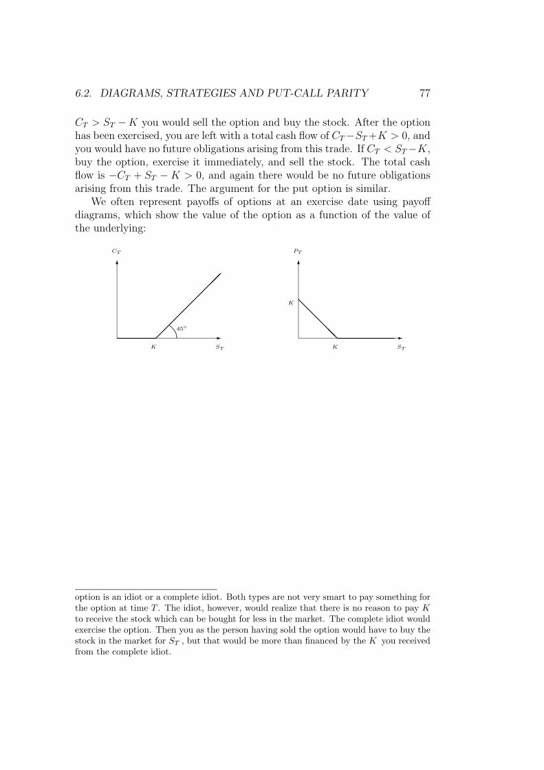
6.2. DIAGRAMS, STRATEGIES AND PUT-CALL PARITY 77
CT > ST −K you would sell the option and buy the stock. After the optionhas been exercised, you are left with a total cash flow of CT−ST +K > 0, andyou would have no future obligations arising from this trade. If CT < ST−K,buy the option, exercise it immediately, and sell the stock. The total cashflow is −CT + ST −K > 0, and again there would be no future obligationsarising from this trade. The argument for the put option is similar.
We often represent payoffs of options at an exercise date using payoffdiagrams, which show the value of the option as a function of the value ofthe underlying:
6
-
CT
K ST
45
6
-
PT
ST
K
K
@@@@@
option is an idiot or a complete idiot. Both types are not very smart to pay something forthe option at time T . The idiot, however, would realize that there is no reason to pay Kto receive the stock which can be bought for less in the market. The complete idiot wouldexercise the option. Then you as the person having sold the option would have to buy thestock in the market for ST , but that would be more than financed by the K you receivedfrom the complete idiot.
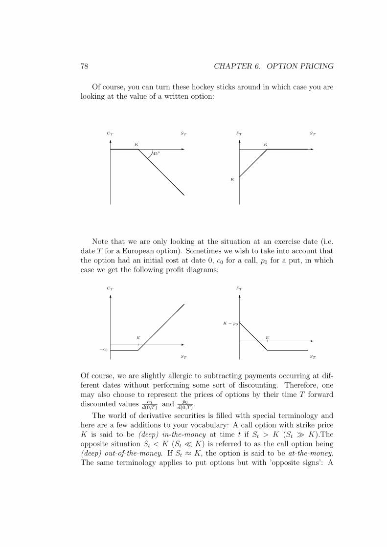
78 CHAPTER 6. OPTION PRICING
Of course, you can turn these hockey sticks around in which case you arelooking at the value of a written option:
6 -
CT
K
ST
45@@@@@@@@
6 -
PT
K
K
ST
Note that we are only looking at the situation at an exercise date (i.e.date T for a European option). Sometimes we wish to take into account thatthe option had an initial cost at date 0, c0 for a call, p0 for a put, in whichcase we get the following profit diagrams:
6
-
CT
K
ST
−c0
6
-
PT
ST
K − p0
K
@@@@@
Of course, we are slightly allergic to subtracting payments occurring at dif-ferent dates without performing some sort of discounting. Therefore, onemay also choose to represent the prices of options by their time T forwarddiscounted values c0
d(0,T )and p0
d(0,T ).
The world of derivative securities is filled with special terminology andhere are a few additions to your vocabulary: A call option with strike priceK is said to be (deep) in-the-money at time t if St > K (St K).Theopposite situation St < K (St K) is referred to as the call option being(deep) out-of-the-money. If St ≈ K, the option is said to be at-the-money.The same terminology applies to put options but with ’opposite signs’: A

6.2. DIAGRAMS, STRATEGIES AND PUT-CALL PARITY 79
put option is in-the-money if St < K.The diagrams we have seen so far considered positions consisting of just
one option. We considered a long position, i.e. a position correspondingto holding the option, and we considered a short position, i.e. a positioncorresponding to having written an option. One of the attractive featuresof options is that they can be combined with positions in other options, theunderlying security and bonds to produce more complicated payoffs thanthose illustrated in the profit diagrams above. We will see examples of thisin the exercises. Note that you should think of the payoff diagram for holdingthe stock and the diagram for holding the bond as being represented by:
6
-
ST
ST
6
-
d(T, T )
ST
1
Until further notice we will assume that the stock does not pay any dividendsin the time interval [0, T ]. This means that if you own the stock you will notreceive any cash unless you decide to sell the stock. With this assumptionand the maintained assumption of frictionless markets we will give some re-strictions on option prices which follow solely from arbitrage considerations.
The most important relation is the so-called put-call parity for Europeanoptions. Consider the portfolio strategy depicted in the table below and theassociated cash flows at time t and time T. Assume that both options areEuropean, expire at date T and have strike price equal to K :
strategy\cashflow date t date T, ST ≤ K date T, ST > K
sell 1 call ct 0 K − STbuy 1 put −pt K − ST 0buy stock −St ST STsell K bonds Kd(t, T ) −K −Ktotal cash flow must be 0 0 0
Note that we have constructed a portfolio which gives a payoff of 0 at timeT no matter what the value of ST . Since the options are European we neednot consider any time points in (t, T ). This portfolio must have price 0, or elsethere would be an obvious arbitrage strategy. If, for example, the portfolio
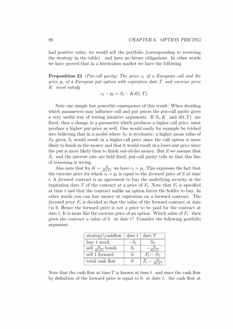
80 CHAPTER 6. OPTION PRICING
had positive value, we would sell the portfolio (corresponding to reversingthe strategy in the table) and have no future obligations. In other wordswe have proved that in a frictionless market we have the following
Proposition 21 (Put-call parity) The price ct of a European call and theprice pt of a European put option with expiration date T and exercise priceK must satisfy
ct − pt = St −Kd(t, T ).
Note one simple but powerful consequence of this result: When decidingwhich parameters may influence call and put prices the put-call parity givesa very useful way of testing intuitive arguments. If St, K and d(t, T ) arefixed, then a change in a parameter which produces a higher call price, mustproduce a higher put-price as well. One would easily for example be trickedinto believing that in a model where ST is stochastic, a higher mean value ofST given St would result in a higher call price since the call option is morelikely to finish in-the-money and that it would result in a lower put price sincethe put is more likely then to finish out-of-the money. But if we assume thatSt and the interest rate are held fixed, put-call parity tells us that this lineof reasoning is wrong.
Also note that for K = Std(t,T )
we have ct = pt. This expresses the fact thatthe exercise price for which ct = pt is equal to the forward price of S at timet. A forward contract is an agreement to buy the underlying security at theexpiration date T of the contract at a price of Ft. Note that Ft is specifiedat time t and that the contract unlike an option forces the holder to buy. Inother words you can lose money at expiration on a forward contract. Theforward price Ft is decided so that the value of the forward contract at datet is 0. Hence the forward price is not a price to be paid for the contract atdate t. It is more like the exercise price of an option. Which value of Ft thengives the contract a value of 0 at date t? Consider the following portfolioargument:
strategy\cashflow date t date T
buy 1 stock −St STsell St
d(t,T )bonds St − St
d(t,T )
sell 1 forward 0 Ft − STtotal cash flow 0 Ft − St
d(t,T )
Note that the cash flow at timeT is known at time t and since the cash flowby definition of the forward price is equal to 0 at date t, the cash flow at

6.3. RESTRICTIONS ON OPTION PRICES 81
date T must be 0 as well. Hence
Ft =St
d(t, T ).
Note that buying a call and selling a put, both with exercise price K andexpiration date T, is equivalent to buying forward at the price K. Thereforethe convention that the forward contract has value 0 at date t is exactlyequivalent to specifying K so that ct = pt.
6.3 Restrictions on option prices
In this section we derive some bounds on call prices which much be satisfiedin frictionless markets. The line of reasoning used may of course be used onput options as well.
Consider a European call option with expiration date T and exercise priceK. Assume that the underlying security does not pay any dividends duringthe life of the option. Then the value of the option ct satisfies
St ≥ ct ≥ max (0, St −Kd(t, T )) . (6.1)
Proof. Clearly, ct ≥ 0.Also, the corresponding put option satisfies pt ≥ 0.Hence
ct ≥ ct − pt = St −Kd(t, T ) (6.2)
where we have used put-call parity. To see that St ≥ ct, assume that St < ctand consider the strategy of buying the stock and selling the option. Thatgives a positive cash flow at time t. If at time T, ST > K and the option isexercised the stock is delivered to the option holder and K is received. Ifthe option is not exercised, the stock can be sold at non-negative value.
It is clear that an American option is more valuable than the correspond-ing European option, hence we note that the price Ct of an American optionalso satisfies Ct ≥ St−Kd(t, T ). If interest rates are positive, i.e. d(t, T ) < 1,this produces the interesting result that the value of the American call is al-ways strictly greater than the immediate exercise value St −K when t < T.This shows the important result that an American option on a non-dividendpaying stock should never be exercised early. Our inequalities above showthat it will be better to sell the option. A corresponding result does not holdfor put options. This is perhaps not so surprising considering that postpon-ing the exercise of a put postpones the receipt of K, whereas delaying theexercise of a call delays the payment of K.
82 CHAPTER 6. OPTION PRICING
Typically, stocks pay dividends and it is important to take this into ac-count when pricing options. It will often be the case that the option contractdoes not take into account whether the underlying stock pays dividends. Adividend payment will normally produce a drop in the stock price and anowner of a call option will be hurt by this drop without receiving the benefitof a dividend. A date t is denoted an ex-dividend date if purchasing the stockat time s < t gives the new owner part in the next dividend payment whereasa purchase at time t does not. For simplicity, we assume in the followingthat the dividend payment takes place at the ex-dividend date. Furthermore,we will assume that the size of the dividend is known some time before thedividend date. In a world with no taxes it ought to be the case then thatthe drop in the stock price around the dividend date is equal to the size ofthe dividend. Assume, for example, that the drop in the stock price is lessthan D. Then buying the stock right before the dividend date for a price ofSt− and selling it for St+ immediately after the dividend date will produce acash flow of St+ +D−St− > 0. This resembles an arbitrage opportunity andit is our explanation for assuming in the following that St− = St+ +D.
Now let us consider the price at time 0 of a European call option on astock which is known to pay one dividend D at time t. Then
c0 ≥ max (0, S0 −Kd(0, T )−Dd(0, t)) .
Again, c0 ≥ 0 is trivial. Assume c0 < S0 − Kd(0, T ) − Dd(0, t). Thenbuy the left hand side and sell the right hand side. At time t, we must paydividend D on the stock we have sold, but that dividend is exactly receivedfrom the D zero coupon bonds with maturity t. At time T the value of theoption we have sold is equal to max (0, ST −K) . The value of the right handside is equal to ST − K. If ST ≥ K the total position is 0.If ST < K thetotal position has value K − ST . Hence we have constructed a positive cashflow while also receiving money initially. This is an arbitrage opportunityand hence we rule out c0 < S0 −Kd(0, T )−Dd(0, t).
There are many possible variations on the dividend theme. If dividendsare not known at time 0 we may assume that they fall within a certaininterval and then use the endpoints of this interval to bound calls and puts.The reader may verify that the maximal dividend is important for boundingcalls and the minimum dividend for bounding put prices.
However, we maintain the assumption of a known dividend and finish thissection by another important observation on the early exercise of Americancalls on dividend paying stocks. Assume that the stock pays a dividend attime t and that we are at time 0 < t. It is then not optimal to exercise theoption at time 0 whereas it may be optimal right before time t. To see that it
6.4. BINOMIAL MODELS FOR STOCK OPTIONS 83
is not optimal at time 0, note that the American option contains as a part ofits rights an option with expiration date s ∈ (0, t), and since this option is anoption on a non-dividend paying stock we know that its value is larger thanS0 −K, which is the value of immediate exercise. Therefore, the Americanoption is also more worth than S0 − K and there is no point in exercisingbefore t. To see that it may be optimal to exercise right before t, considera firm which pays a liquidating dividend to all its shareholders. The stockwill be worthless after the liquidation and so will the call option. Certainly,the option holder is better off to exercise right before the dividend date toreceive part of the liquidating dividend.
The picture is much more complicated for puts. In the next section wewill see how to compute prices for American puts in binomial models andthis will give us the optimal exercise strategy as well.
6.4 Binomial models for stock options
In this section we will go through the binomial model for pricing stock op-tions. Our primary focus is the case where the underlying security is anon-dividend paying stock but it should be transparent that the binomialframework is highly flexible and will easily handle the pricing and hedgingof derivative securities with more complicated underlying securities.
We consider a model with T periods and assume throughout that thefollowing two securities trade:
1. A money market account with a constant spot rate process ρ. Let1 + ρt = R, where R ≥ 1. Hence we have for s < t
Rs,t = Rt−s.
2. A stock2 S , which pays no dividends3 , whose price at time 0 is S0 andwhose evolution under the measure P is described in the tree (wherewe have assumed that u > R > d > 0) shown below.
2Since there is only one stock we will write S instead of S1.3To comply with the mathematical model of the previous chapter we should actually
say that the stock pays a liquidating dividend of ST at time T . We will however speak ofST as the price at time T of the stock.
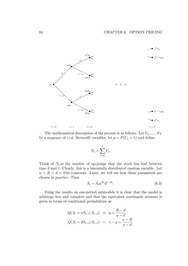
84 CHAPTER 6. OPTION PRICING
t = 0 t = 1 t = 2 t = T
S0s
p
suS0
@@@@@@
1− p sdS0
su2S0
p
PP
HHH
HHHsudS0
1− p PP
sduS0
p
PP
1− p
HHHHHHsd2S0
PP
s` dT S0
s dT−1uS0
s` uT−1dS0
s uTS0
c c c
The mathematical description of the process is as follows: Let U1, . . . , UTbe a sequence of i.i.d. Bernoulli variables, let p = P (U1 = 1) and define
Nt =t∑i=1
Ui.
Think of Nt as the number of up-jumps that the stock has had betweentime 0 and t. Clearly, this is a binomially distributed random variable. Letu > R > d > 0 be constants. Later, we will see how these parameters arechosen in practice. Then
St = S0uNtdt−Nt . (6.3)
Using the results on one-period submodels it is clear that the model isarbitrage free and complete and that the equivalent martingale measure isgiven in terms of conditional probabilities as
Q(St = uSt−1|St−1) ≡ q =R− du− d
Q(St = dSt−1|St−1) = 1− q =u−Ru− d
.
6.5. PRICING THE EUROPEAN CALL 85
6.5 Pricing the European call
We now have the martingale measure Q in place and hence the value at timet of a European call with maturity T is given in an arbitrage-free model by
Ct =1
RT−tEQ (max(0, ST −K) |Ft ) .
Using this fact we get the following
Proposition 22 Let the stock and money market account be as described insection 6.4. Then the price of a European call option with exercise price Kand maturity date T is given as
Ct =1
RT−t
T−t∑i=0
(T − ti
)qi(1− q)T−t−i max(0, Stu
idT−t−i −K).
Proof. Since the money market account and S0 are deterministic, we havethat we get all information by observing just stock-prices, or equivalently theU ’s, i.e. Ft = σ(S1, . . . , St) = σ(U1, . . . , Ut). By using (6.3) twice we canwrite
ST = Stu(NT−Nt)d(T−t)−(NT−Nt) = Stu
Zd(T−t)−Z ,
where Z = NT − Nt =∑T
j=t+1 UjQ∼ bi(q; (T − t)), and Z is independent of
Ft (because the U ’s are independent). Therefore
RT−tCt = EQ((ST −K)+|Ft) = EQ((StuZd(T−t)−Z −K)+|Ft).
At this point in the narrative we need something called “the useful rule”. Itstates the following: Suppose we are given a function f : R2 7→ R, a σ-algebraF , an F -measurable random variable X and a random variable Y that isindependent of F . Define the function g : R 7→ R by g(x) = E(f(x, Y )).Then E(f(X,Y )|F) = g(X). We then use this in the above expression withSt playing the role of X, Z as Y , and f(x, y) = (xuyd(T−t)−y−K)+. By usingthe general transformation rule for discrete random variables E(h(Y )) =∑
yih(yi)P (Y = yi), and the fact that Z is Q-binomially distributed we get
in the notation of “the useful rule” that
g(x) =T−t∑i=0
(T − ti
)qi(1− q)(T−t)−i(xuid(T−t)−i −K)+,
and the desired result follows.
86 CHAPTER 6. OPTION PRICING
We rewrite the expression for C0 using some handy notation. Let a bethe smallest number of upward jumps needed for the option to finish in themoney, i.e.
a = minj∈Nj|S0u
jdT−j > K
= minj∈Nj|j lnu+ (T − j) ln d > ln(K/S0)
= minj∈Nj|j > ln(K/(S0d
T ))/ ln(u/d)
=
ln(
KS0dT
)ln(ud
)+ 1.
Letting
Ψ(a;T, q) =T∑i=a
(Ti
)qi(1− q)T−i,
we may write (you may want to check the first term on the RHS)
C0 = S0Ψ (a;T, q′)− K
RTΨ (a;T, q) (6.4)
whereq′ =
u
Rq.
Using put-call parity gives us the price of the European put:
Corollary 23 The price of a European put option with T periods to matu-rity, exercise price T and the stocks as underlying security has a price at time0 given by
P0 =K
RT(1−Ψ (a;T, q))− S0 (1−Ψ (a;T, q′))
Note that our option pricing formulae use T to denote the number ofperiods until maturity. Later, we will be more explicit in relating this toactual calendar time.
6.6 Hedging the European call
We have already seen in a two period model how the trading strategy repli-cating a European call option may be constructed. In this section we simplystate the result for the case with T periods and we then note an interesting
6.6. HEDGING THE EUROPEAN CALL 87
way of expressing the result. We consider the case with a money marketaccount and one risky asset S and assume that the market is complete andarbitrage-free. The European call option has a payout at maturity of
δcT = max(ST −K, 0).
Proposition 24 A self-financing trading strategy replicating the dividendprocess of the option from time 1 to T is constructed recursively as follows:Find φT−1 = (φ0
T−1, φ1T−1) such that
φ0T−1R + φ1
T−1ST = δcT .
For t = T − 2, T − 3, . . . , 1 find φt = (φ0t , φ
1t ) such that
φ0tR + φ1
tSt+1 = φ0t+1 + φ1
t+1St+1.
The trading strategy is self-financing by definition, replicates the calland its initial price of φ0
0 + φ10S0 is equal to the arbitrage-free price of the
option. We may easily extend to the case where both the underlying and thecontingent claim have dividends other than the one dividend of the optionconsidered above. In that case the procedure is the following:Find φT−1 =(φ0
T−1, φ1T−1) such that
φ0T−1R + φ1
T−1(ST + δT ) = δcT .
For t = T − 2, T − 3, . . . , 1 find φt = (φ0t , φ
1t ) such that
φ0tR + φ1
t (St+1 + δt+1) = φ0t+1 + φ1
t+1St+1 + δct+1.
In this case the trading strategy is not self-financing in general but it matchesthe dividend process of the contingent claim, and the initial price of thecontingent claim is still φ0
0 + φ10S0.
An additional insight into the hedging strategy is given by the propositionbelow.
Recall the notation
St =StR0,t
for the discounted price process of the stock. Let Ct denote the price processof a contingent claim whose dividend process is δc and let
Ct =CtR0,t
δc
t =δctR0,t
88 CHAPTER 6. OPTION PRICING
denote the discounted price and dividend processes of the contingent claim.Define the conditional covariance under the martingale measure Q as follows:
CovQ (Xt+1, Yt+1 |Ft ) = EQ ((Xt+1 −Xt) (Yt+1 − Yt)| Ft)
One may then show the following (but we will omit the proof):
Proposition 25 Assume that the stock pays no dividends during the life ofthe option. The hedging strategy which replicates δc is computed as follows:
φ1t =
CovQ(St+1, Ct+1 + δ
c
t+1
∣∣∣Ft)VARQ
(St+1 |Ft
) t = 0, 1, . . . , T − 1
φ0t = Ct − φ1
t St t = 0, 1, . . . , T − 1
Note the similarity with regression analysis! We will not go further intothis at this stage. But this way of looking at hedging is important whendefining so-called risk minimal trading strategies in incomplete markets.
The number of stocks held at time t in the replicating strategy is calledthe hedge ratio. The hedge ratio for a call option is a number between 0 and1, and it is larger the more in-the-money the call is.
6.7 Recombining tree representation
If the number of time periods T is large it the tree representing the stockprice evolution grows very rapidly. The number of nodes at time t is equalto 2t, and since for example 220 = 1048576 we see that when you implementthis model in a spreadsheet and you wish to follow Ct and the associatedhedging strategy over time, you may soon run out of space. Fortunately, inmany cases there is a way around this problem: If your security price processis Markov and the contingent claim you wish to price is path-independent,you can use a recombining tree to do all of your calculations. Let us lookat each property in turn4: The process S is a Markov chain under Q if itsatisfies
Q(St+1 = st+1 |St = st, . . . S1 = s1, S0 = s0 ) = Q(St+1 = st+1 |St = st )
for all t and all (st+1, st, . . . , s1, s0). Intuitively, standing at time t, the currentvalue of the process st is sufficient for describing the distribution of the
4These properties are interesting to consider for the stock only since the money marketaccount trivially has all nice properties discussed in the following.
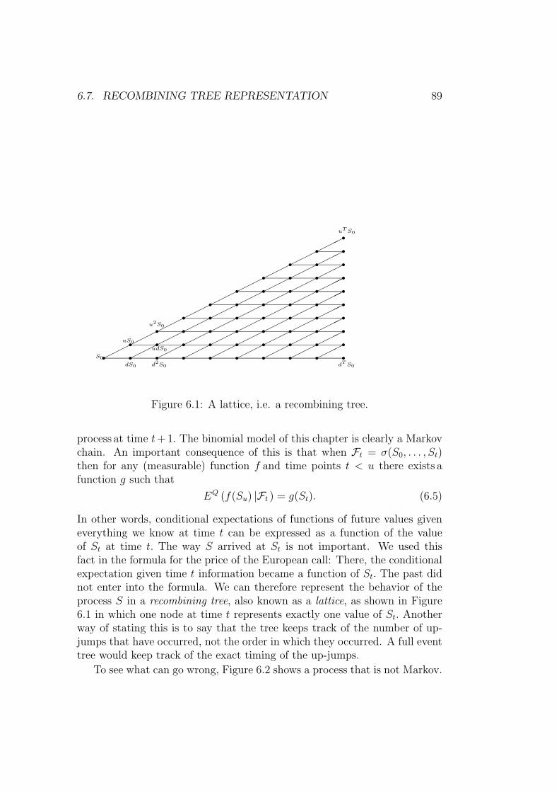
6.7. RECOMBINING TREE REPRESENTATION 89
r rr rr rr rr r
r rr rr rr rr
r rr rr rr r
r rr rr rr
r rr rr r
r rr rr
r rr r
r rr
r rrS0
uS0
dS0
u2S0
udS0
d2S0
uT S0
dTS0
Figure 6.1: A lattice, i.e. a recombining tree.
process at time t+ 1. The binomial model of this chapter is clearly a Markovchain. An important consequence of this is that when Ft = σ(S0, . . . , St)then for any (measurable) function f and time points t < u there exists afunction g such that
EQ (f(Su) |Ft ) = g(St). (6.5)
In other words, conditional expectations of functions of future values giveneverything we know at time t can be expressed as a function of the valueof St at time t. The way S arrived at St is not important. We used thisfact in the formula for the price of the European call: There, the conditionalexpectation given time t information became a function of St. The past didnot enter into the formula. We can therefore represent the behavior of theprocess S in a recombining tree, also known as a lattice, as shown in Figure6.1 in which one node at time t represents exactly one value of St. Anotherway of stating this is to say that the tree keeps track of the number of up-jumps that have occurred, not the order in which they occurred. A full eventtree would keep track of the exact timing of the up-jumps.
To see what can go wrong, Figure 6.2 shows a process that is not Markov.
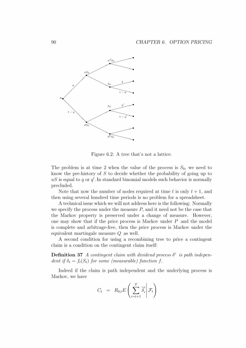
90 CHAPTER 6. OPTION PRICING
S0
rq
@@@@@@
1− q
ruS0
HHHHHH
rdS0HH
HHHH
ru2S0
XXXXXX
rS0
XXXXXX
q
1− q
rS0
XXXXXX
q′
1− q′
rd2S0XXXXXXrrrrrrrr
Figure 6.2: A tree that’s not a lattice.
The problem is at time 2 when the value of the process is S0, we need toknow the pre-history of S to decide whether the probability of going up touS is equal to q or q′. In standard binomial models such behavior is normallyprecluded.
Note that now the number of nodes required at time t is only t+ 1, andthen using several hundred time periods is no problem for a spreadsheet.
A technical issue which we will not address here is the following: Normallywe specify the process under the measure P, and it need not be the case thatthe Markov property is preserved under a change of measure. However,one may show that if the price process is Markov under P and the modelis complete and arbitrage-free, then the price process is Markov under theequivalent martingale measure Q as well.
A second condition for using a recombining tree to price a contingentclaim is a condition on the contingent claim itself:
Definition 37 A contingent claim with dividend process δc is path indepen-dent if δt = ft(St) for some (measurable) function f.
Indeed if the claim is path independent and the underlying process isMarkov, we have
Ct = R0,tE
(T∑
i=t+1
δc
i
∣∣∣∣∣Ft)
6.8. THE BINOMIAL MODEL FOR AMERICAN PUTS 91
= R0,tE
(T∑
i=t+1
fi(Si)
∣∣∣∣∣Ft)
= R0,tE
(T∑
i=t+1
fi(Si)
∣∣∣∣∣St)
and the last expression is a function of St by the Markov property. A Euro-pean option with expiration date T is path-independent since its only divi-dend payment is at time T and is given as max(ST −K, 0).
The Asian option is an example of a contingent claim which is not path-independent. An Asian option on the stock, initiated at time 0, expirationdate T and exercise price K has a payoff at date T given by
CasianT = max
(0,
(1
T + 1
T∑t=0
St
)−K
)Hence the average of the stock price over the period determines the optionprice. Clearly, ST is not sufficient to describe the value of the Asian optionat maturity. To compute the average value one needs the whole path of S.As noted above, even in a binomial model keeping track of the whole pathfor, say, 50 periods becomes intractable.
6.8 The binomial model for American puts
We describe in this section a simple way of pricing the American put optionin a binomial model. Strictly speaking, an American put is not a contingentclaim in the sense we have thought of contingent claims earlier. Generally, wehave thought of contingent claims as random variables or sometimes as pro-cesses but a put is actually not specified until an exercise policy is associatedwith the put. What we will do in the following is to simultaneously solvefor the optimal exercise policy, i.e. the one that maximizes the expected,discounted value of the cash flows under the martingale measure, and theprice of the option. The argument given is not a proof but should be enoughto convince the reader that the right solution is obtained (it is fairly easy toshow that another exercise policy will create arbitrage opportunities for theoption writer).
The value of an American put at its maturity is easy enough:5
PT = max(0, K − ST ). (6.6)5Or is it? As it stands Pt is really the value at time t given that the put has not been
exercised at times 0, 1, t − 1. But that will most often be exactly what we are interestedin; if we exercised the put to years ago, we really don’t care about it anymore.
92 CHAPTER 6. OPTION PRICING
Now consider the situation one period before maturity. If the put hasnot been exercised at that date, the put option holder has two possibilities:Exercise the put at time T − 1 or hold the put to maturity. The value ofholding the put to maturity is given as the discounted (back to time T − 1)value of (6.6), whereas the value at time T − 1 of exercising immediately isK − ST−1 something only to be considered of course if K > ST−1. Clearly,the put option holder has a contract whose value is given by the maximalvalue of these two strategies, i.e.6
PT−1 = max
(K − ST−1, E
Q
(PTR
∣∣∣∣FT−1
)).
Now continue in this fashion by working backwards through the tree to obtainthe price process of the American put option given by the recursion
Pt−1 = max
(K − St−1, E
Q
(PtR
∣∣∣∣Ft−1
))t = 1, . . . , T.
Once this price process is given we see that the optimal exercise strategy isto exercise the put the first time t for which
K − St > EQ
(Pt+1
R
∣∣∣∣Ft) .This way of thinking is easily translated to American call options on dividendpaying stocks for which early exercise is something to consider.
6.9 Implied volatility
We assume in this section that the Black-Scholes formula is known to thereader: The price at time t of a European call option maturing at time T ,when the exercise price is K and the underlying security is a non-dividendpaying stock with a price of St, is given in the Black-Scholes framework by
Ct = StΦ (d1)−Ke−r(T−t)Φ (d2)
where
d1 =log(StK
)+(r + 1
2σ2)
(T − t)σ√T − t
andd2 = d1 − σ
√T − t
6We do not need 0 in the list of arguments of max since positivity is assured by PT ≥ 0.
6.9. IMPLIED VOLATILITY 93
where Φ is the cumulative distribution function of a standard normal distri-bution.
Consider the Black-Scholes formula for the price of a European call on anunderlying security whose value at time 0 is S0: Recall that Φ is a distributionfunction, hence Φ(x) → 1 as x → ∞ and Φ(x) → 0 as x → −∞. Assumethroughout that T > 0. From this it is easy to see that c0 → S0 as σ →∞. By considering the cases S0 < K exp(−rT ) , S0 = K exp(−rT ) andS0 > K exp(−rT ) separately, it is easy to see that as σ → 0, we havec0 → max (0, S0 −K exp(−rT )) . By differentiating c0 with respect to σ,one may verify that c0 is strictly increasing in σ. Therefore, the followingdefinition makes sense:
Definition 38 Given a security with price S0. Assume that the risk freerate (i.e. the rate of the money market account) is equal to r. Assume thatthe price of a call option on the security with exercise price K and time tomaturity T is observed to have a price of cobs with
max(0, S0 −K exp(−rT )) < cobs < S0.
Then the implied volatility of the option is the unique value of σ for which
c0(S0, K, T, σ, r) = cobs.
In other words, the implied volatility is the unique value of the volatilitywhich makes the Black-Scholes model ’fit’ cobs. Clearly, we may also asso-ciate an implied volatility to a put option whose observed price respects theappropriate arbitrage bounds.
A very important reason for the popularity of implied volatility is theway in which it allows a transformation of option prices which are hard tocompare into a common scale. Assume that the price of a stock is 100 andthe riskfree rate is 0.1. If one observed a price of 9.58 on a call option on thestock with exercise price 100 and 6 months to maturity and a price of 2.81on a put option on the stock with exercise price 95 and 3 months to maturitythen it would require a very good knowledge of the Black-Scholes model tosee if one price was in some way higher than the other. However, if we aretold that the implied volatility of the call is 0.25 and the implied volatilityof the put is 0.30, then at least we know that compared to the Black-Scholesmodel, the put is more expensive than the call. This way of comparing is infact so popular that traders in option markets typically do not quote pricesin (say) dollars, but use ’vols’ instead.
If the Black-Scholes model were true the implied volatility of all optionswritten on the same underlying security should be the same, namely equal
94 CHAPTER 6. OPTION PRICING
to the volatility of the stock and this volatility would be a quantity we couldestimate from historical data. In short, in a world where the Black-Scholesmodel holds, historical volatility (of the stock) is equal to implied volatility(of options written on the stock). In practice this is not the case - afterall the Black-Scholes model is only a model. The expenses of hedging anoption depend on the volatility of the stock during the life of the option.If, for example, it is known that, after a long and quiet period, importantnews about the underlying stock will arrive during the life of the option, theoption price should reflect the fact that future fluctuations in the stock pricemight be bigger than the historical ones. In this case the implied volatilitywould be higher than the historical.
However, taking this knowledge of future volatility into account one couldstill imagine that all implied volatilities of options on the same underlyingwere the same (and equal to the ’anticipated’ volatility). In practice this isnot observed either. To get an idea of why, we consider the notion of portfolioinsurance.
6.10 Portfolio insurance, implied volatility and
crash fears
Consider a portfolio manager who manages a portfolio which is diversifiedso that the value of her portfolio follows that of the market stock index.Assume that the value of her portfolio is 1000 times the value of the indexwhich is assumed to be at 110. The portfolio manager is very worried aboutlosing a large portion of the value of the portfolio over the next year - shethinks that there is a distinct possibility that the market will crash. On theother hand she is far from certain. If she were certain, she could just movethe money to a bank at a lower but safer expected return than in the stockmarket. But she does not want to exclude herself from the gains that a surgein the index would bring. She therefore decides to buy portfolio insurancein such a way that the value of her portfolio will never fall below a level of(say) 90.000. More specifically, she decides to buy 1000 put options with oneyear to maturity and an exercise price of 90 on the underlying index. Nowconsider the value of the portfolio after a year as a function of the level ofthe index ST :
value of index ST ≥ 90 ST < 90value of stocks ST × 1000 ST × 1000value of puts 0 1000× (90− ST )
total value ST × 1000 > 90.000 90.000
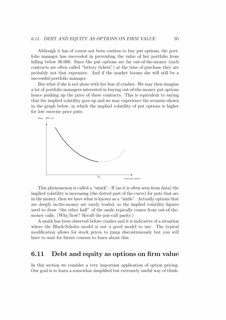
6.11. DEBT AND EQUITY AS OPTIONS ON FIRM VALUE 95
Although it has of course not been costless to buy put options, the port-folio manager has succeeded in preventing the value of her portfolio fromfalling below 90.000. Since the put options are far out-of-the-money (suchcontracts are often called “lottery tickets”) at the time of purchase they areprobably not that expensive. And if the market booms she will still be asuccessful portfolio manager.
But what if she is not alone with her fear of crashes. We may then imaginea lot of portfolio managers interested in buying out-of-the-money put optionshence pushing up the price of these contracts. This is equivalent to sayingthat the implied volatility goes up and we may experience the scenario shownin the graph below, in which the implied volatility of put options is higherfor low exercise price puts:
-exercise price
6
Imp . BS-vol.
S0
This phenomenon is called a “smirk”. If (as it is often seen from data) theimplied volatility is increasing (the dotted part of the curve) for puts that arein the money, then we have what is known as a “smile”. Actually options thatare deeply in-the-money are rarely traded, so the implied volatility figuresused to draw “the other half” of the smile typically comes from out-of-the-money calls. (Why/how? Recall the put-call parity.)
A smirk has been observed before crashes and it is indicative of a situationwhere the Black-Scholes model is not a good model to use. The typicalmodification allows for stock prices to jump discontinuously but you willhave to wait for future courses to learn about this.
6.11 Debt and equity as options on firm value
In this section we consider a very important application of option pricing.Our goal is to learn a somewhat simplified but extremely useful way of think-
96 CHAPTER 6. OPTION PRICING
ing about a firm which is financed by debt and equity (see below). A fun-damental assumption in this section is that a firm has a market value givenby a stochastic process V. In Arrow-Debreu economies in which we knowprices and production plans adopted by the firms, it is easy to define thevalue of a firm as the (net) value of its production. In reality things are ofcourse a lot more complicated. It is hard to know, for example, what thevalue of Novo-Nordisk is - i.e. what is the market value of the firm’s assets(including know-how, goodwill etc.). Part of the problem is of course that itis extremely difficult to model future prices and production levels. But in asense the actual value does not matter for this section in that the ’sign’ ofthe results that we derive does not depend on what the value of the firm is -only the ”magnitude’ does.
The fundamental simplification concerns the capital structure of the firm.Assume that the firm has raised capital to finance its activities in two ways:It has issued stocks (also referred to as equity) and debt. The debt consistsof zero coupon bonds with face value D maturing at time T. Legally whatdistinguishes the debt holders from the stock holders is the following: Thestock holders control the firm and they decide at time T whether the firmshould repay its debt to the bondholders. If the bondholders are not repaidin full they can force the firm into bankruptcy and take over the remainingassets of the firm (which means both controlling and owning it). The stockswill then be worthless. If the stockholders pay back D at maturity to thebondholders, they own the firm entirely. They may then of course decide toissue new debt to finance new projects but we will not worry about that now.
It is clear that the stockholders will have an interest in repaying thebondholders precisely when VT > D. Only then will the expense in payingback the debt be more than outweighed by the value of the firm. If VT < D(and there are no bankruptcy costs) the stockholders will default on theirdebt, the firm will go into bankruptcy and the bondholders will take over.In short, we may write the value of debt and equity at time T as
BT = min (D,VT ) = D −max (D − VT , 0)
ST = max(VT −D, 0).
In other words, we may think of equity as a call option on the value ofthe firm and debt as a zero coupon bond minus a put option on the valueof the firm. Assuming then that V behaves like the underlying security inthe Black-Scholes model and that there exists a money market account withinterest rate r, we can use the Black-Scholes model to price debt and equityat time 0 :
B0 = D exp(−rT )− p0(V0, D, T, σ, r)

6.11. DEBT AND EQUITY AS OPTIONS ON FIRM VALUE 97
S0 = c0(V0, D, T, σ, r)
where p0, c0 are Black-Scholes put and call functions.Let us illustrate a potential conflict between stockholders and bondholders
in this model. Assume that at time 0 the firm has the possibility of adoptinga project which will not alter the value of the firm at time 0, but which willhave the effect of increasing the volatility of the process V. Since both thevalue of the call and the put increases when σ increases we see that thestockholders will like this project since it increases the value of the equitywhereas the bondholders will not like the project since the put option whichthey have in a sense written will be a greater liability to them. This is a veryclear and very important illustration of so-called asset substitution, a sourceof conflict which exists between stock-and bondholders of a firm. This setupof analyzing the value of debt and equity is useful in a number of contextsand you should make sure that you understand it completely. We will returnto this towards the end of the course when discussing corporate finance.

98 CHAPTER 6. OPTION PRICING
Chapter 7
The Black-Scholes formula
7.1 Black-Scholes as a limit of binomial mod-
els
So far we have not specified the parameters p, u, d and R which are of coursecritical for the option pricing model. Also, it seems reasonable that if wewant the binomial model to be a realistic model for stock prices over a certaininterval of time we should use a binomial model which divides the (calendar)time interval into many sub-periods. In this chapter we will first show that ifone divides the interval into finer and finer periods and choose the parameterscarefully, the value of the option converges to a limiting formula, the Black-Scholes formula, which was originally derived in a continuous time framework.We then describe that framework and show how to derive the formula in it.
Our starting point is an observed stock price whose logarithmic returnsatisfies
EP
[ln
(StSt−1
)]= µ
and
V P
(ln
(StSt−1
))= σ2,
where St is the price of the stock t years after the starting date 0. Also,assume that the money market account has a continuously compounded re-turn of r, i.e. an amount of 1 placed in the money market account growsto exp(r) in one year. Note that since RT = exp (T ln (R)), a yearly rate ofR = 1.1 (corresponding to a yearly rate of 10%) translates into the contin-uous compounding analogue r = ln (1.1) and this will be a number smallerthan 0.1.
99
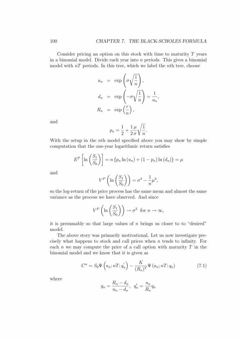
100 CHAPTER 7. THE BLACK-SCHOLES FORMULA
Consider pricing an option on this stock with time to maturity T yearsin a binomial model. Divide each year into n periods. This gives a binomialmodel with nT periods. In this tree, which we label the nth tree, choose
un = exp
(σ
√1
n
),
dn = exp
(−σ√
1
n
)=
1
un,
Rn = exp( rn
),
and
pn =1
2+
1
2
µ
σ
√1
n.
With the setup in the nth model specified above you may show by simplecomputation that the one-year logarithmic return satisfies
EP
[ln
(S1
S0
)]= n pn ln (un) + (1− pn) ln (dn) = µ
and
V P
(ln
(S1
S0
))= σ2 − 1
nµ2,
so the log-return of the price process has the same mean and almost the samevariance as the process we have observed. And since
V P
(ln
(S1
S0
))→ σ2 for n→∞,
it is presumably so that large values of n brings us closer to to “desired”model.
The above story was primarily motivational. Let us now investigate pre-cisely what happens to stock and call prices when n tends to infinity. Foreach n we may compute the price of a call option with maturity T in thebinomial model and we know that it is given as
Cn = S0Ψ(an;nT ; q
′
n
)− K
(Rn)TΨ (an;nT ; qn) (7.1)
where
qn =Rn − dnun − dn
, q′n =unRn
qn
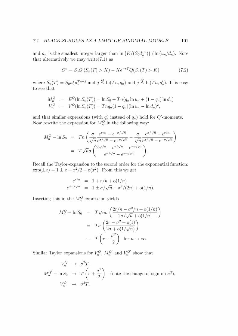
7.1. BLACK-SCHOLES AS A LIMIT OF BINOMIAL MODELS 101
and an is the smallest integer larger than ln(K/(S0d
Tnn ))/ ln (un/dn). Note
that alternatively we may write(7.1) as
Cn = S0Q′(Sn(T ) > K)−Ke−rTQ(Sn(T ) > K) (7.2)
where Sn(T ) = S0ujnd
Tn−jn and j
Q∼ bi(Tn, qn) and jQ′∼ bi(Tn, q′n). It is easy
to see that
MQn := EQ(lnSn(T )) = lnS0 + Tn(qn lnun + (1− qn) ln dn)
V Qn := V Q(lnSn(T )) = Tnqn(1− qn)(lnun − ln dn)2,
and that similar expressions (with q′n instead of qn) hold for Q′-moments.Now rewrite the expression for MQ
n in the following way:
MQn − lnS0 = Tn
(σ√n
er/n − e−σ/√n
eσ/√n − e−σ/
√n− σ√
n
eσ/√n − er/n
eσ/√n − e−σ/
√n
)= T
√nσ
(2er/n − eσ/
√n − e−σ/
√n
eσ/√n − e−σ/
√n
).
Recall the Taylor-expansion to the second order for the exponential function:exp(±x) = 1± x+ x2/2 + o(x2). From this we get
er/n = 1 + r/n+ o(1/n)
e±σ/√n = 1± σ/
√n+ σ2/(2n) + o(1/n).
Inserting this in the MQn expression yields
MQn − lnS0 = T
√nσ
(2r/n− σ2/n+ o(1/n)
2σ/√n+ o(1/n)
)= Tσ
(2r − σ2 + o(1)
2σ + o(1/√n)
)→ T
(r − σ2
2
)for n→∞.
Similar Taylor expansions for V Qn , MQ′
n and V Q′n show that
V Qn → σ2T,
MQ′
n − lnS0 → T
(r +
σ2
2
)(note the change of sign on σ2),
V Q′
n → σ2T.
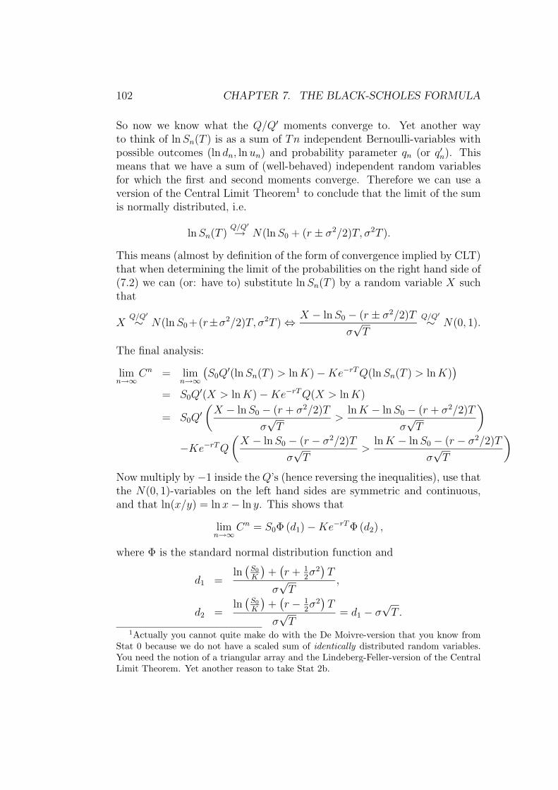
102 CHAPTER 7. THE BLACK-SCHOLES FORMULA
So now we know what the Q/Q′ moments converge to. Yet another wayto think of lnSn(T ) is as a sum of Tn independent Bernoulli-variables withpossible outcomes (ln dn, lnun) and probability parameter qn (or q′n). Thismeans that we have a sum of (well-behaved) independent random variablesfor which the first and second moments converge. Therefore we can use aversion of the Central Limit Theorem1 to conclude that the limit of the sumis normally distributed, i.e.
lnSn(T )Q/Q′→ N(lnS0 + (r ± σ2/2)T, σ2T ).
This means (almost by definition of the form of convergence implied by CLT)that when determining the limit of the probabilities on the right hand side of(7.2) we can (or: have to) substitute lnSn(T ) by a random variable X suchthat
XQ/Q′∼ N(lnS0 +(r±σ2/2)T, σ2T )⇔ X − lnS0 − (r ± σ2/2)T
σ√T
Q/Q′∼ N(0, 1).
The final analysis:
limn→∞
Cn = limn→∞
(S0Q
′(lnSn(T ) > lnK)−Ke−rTQ(lnSn(T ) > lnK))
= S0Q′(X > lnK)−Ke−rTQ(X > lnK)
= S0Q′(X − lnS0 − (r + σ2/2)T
σ√T
>lnK − lnS0 − (r + σ2/2)T
σ√T
)−Ke−rTQ
(X − lnS0 − (r − σ2/2)T
σ√T
>lnK − lnS0 − (r − σ2/2)T
σ√T
)Now multiply by −1 inside the Q’s (hence reversing the inequalities), use thatthe N(0, 1)-variables on the left hand sides are symmetric and continuous,and that ln(x/y) = lnx− ln y. This shows that
limn→∞
Cn = S0Φ (d1)−Ke−rTΦ (d2) ,
where Φ is the standard normal distribution function and
d1 =ln(S0
K
)+(r + 1
2σ2)T
σ√T
,
d2 =ln(S0
K
)+(r − 1
2σ2)T
σ√T
= d1 − σ√T .
1Actually you cannot quite make do with the De Moivre-version that you know fromStat 0 because we do not have a scaled sum of identically distributed random variables.You need the notion of a triangular array and the Lindeberg-Feller-version of the CentralLimit Theorem. Yet another reason to take Stat 2b.
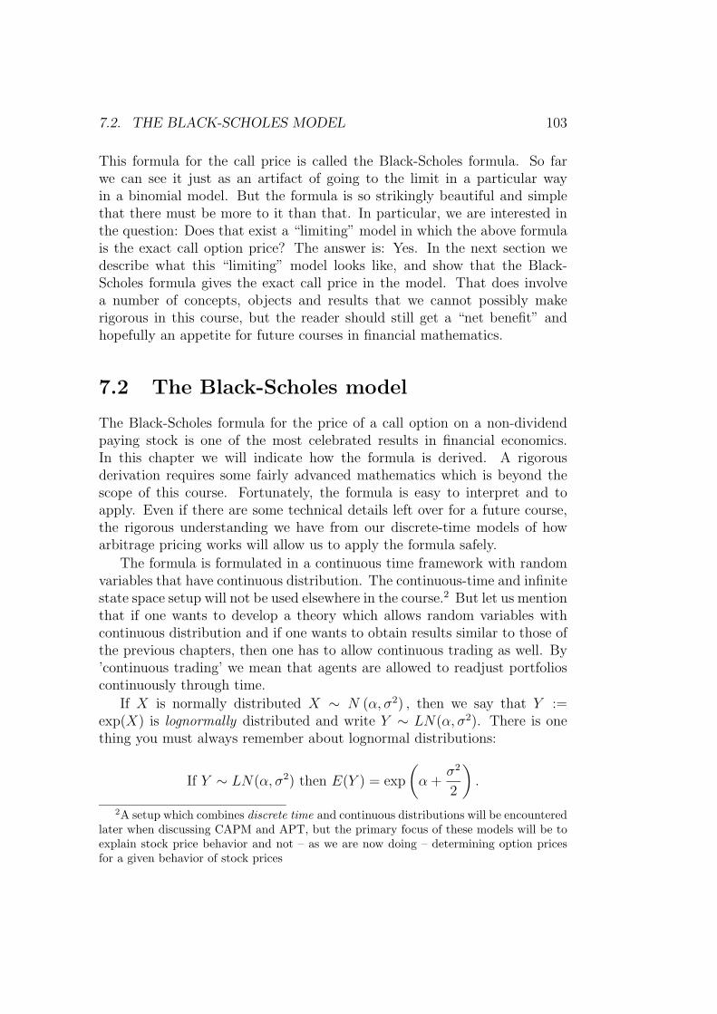
7.2. THE BLACK-SCHOLES MODEL 103
This formula for the call price is called the Black-Scholes formula. So farwe can see it just as an artifact of going to the limit in a particular wayin a binomial model. But the formula is so strikingly beautiful and simplethat there must be more to it than that. In particular, we are interested inthe question: Does that exist a “limiting” model in which the above formulais the exact call option price? The answer is: Yes. In the next section wedescribe what this “limiting” model looks like, and show that the Black-Scholes formula gives the exact call price in the model. That does involvea number of concepts, objects and results that we cannot possibly makerigorous in this course, but the reader should still get a “net benefit” andhopefully an appetite for future courses in financial mathematics.
7.2 The Black-Scholes model
The Black-Scholes formula for the price of a call option on a non-dividendpaying stock is one of the most celebrated results in financial economics.In this chapter we will indicate how the formula is derived. A rigorousderivation requires some fairly advanced mathematics which is beyond thescope of this course. Fortunately, the formula is easy to interpret and toapply. Even if there are some technical details left over for a future course,the rigorous understanding we have from our discrete-time models of howarbitrage pricing works will allow us to apply the formula safely.
The formula is formulated in a continuous time framework with randomvariables that have continuous distribution. The continuous-time and infinitestate space setup will not be used elsewhere in the course.2 But let us mentionthat if one wants to develop a theory which allows random variables withcontinuous distribution and if one wants to obtain results similar to those ofthe previous chapters, then one has to allow continuous trading as well. By’continuous trading’ we mean that agents are allowed to readjust portfolioscontinuously through time.
If X is normally distributed X ∼ N (α, σ2) , then we say that Y :=exp(X) is lognormally distributed and write Y ∼ LN(α, σ2). There is onething you must always remember about lognormal distributions:
If Y ∼ LN(α, σ2) then E(Y ) = exp
(α +
σ2
2
).
2A setup which combines discrete time and continuous distributions will be encounteredlater when discussing CAPM and APT, but the primary focus of these models will be toexplain stock price behavior and not – as we are now doing – determining option pricesfor a given behavior of stock prices
104 CHAPTER 7. THE BLACK-SCHOLES FORMULA
If you have not seen this before, then you are strongly urged to check it.(With that result you should also be able to see why there is no need touse “brain RAM” remembering the variance of a lognormally distributedvariable.) Often the lognormal distribution is preferred as a model for stockprice distributions since it conforms better with the institutional fact thatprices of a stock are non-negative and the empirical observation that thelogarithm of stock prices seem to show a better fit to a normal distributionthan do prices themselves. However, specifying a distribution of the stockprice at time t, say, is not enough. We need to specify the whole process ofstock prices, i.e. we need to state what the joint distribution (St1 , . . . , StN )is for any 0 ≤ t1 < . . . < tN . To do this the following object is central.
Definition 39 A (standard) Brownian motion ((S)BM) is a stochastic pro-cess B = (Bt)t∈[0;∞[ -i.e. a sequence of random variables indexed by t suchthat:
1. B0 = 0
2. Bt −Bs ∼ N (0, t− s) ∀ s < t
3. B has independent increments, i.e. for every N and a set of N timepoints t1 < . . . < tN , Bt1 , Bt2 − Bt1 , Bt3 − Bt2 , . . . , BtN − BtN−1
areindependent random variables.
That these demands on a process can be satisfied simultaneously is nottrivial. But don’t worry, Brownian motion does exist. It is, however, a fairly“wild” object. The sample paths (formally the mapping t 7→ Bt and intu-itively simply the graph you get by plotting “temperature/stock price/. . .”against time) of BM are continuous everywhere but differentiable nowhere.The figure shows a simulated sample path of a BM and should give an indica-
7.2. THE BLACK-SCHOLES MODEL 105
tion of this.
A useful fact following from the independent increment property is thatfor any measurable f : R→R for which E [|f (Bt −Bs)|] <∞ we have
E [f (Bt −Bs)| Fs] = E [f (Bt −Bs)] (7.3)
where Fs = σ Bu : 0 ≤ u ≤ s .The fundamental assumption of the Black-Scholes model is that the stock
price can be represented by
St = S0 exp (αt + σBt) (7.4)
where Bt is a SBM. Such a process is called a geometric BM (with drift).Furthermore, it assumes that there exists a riskless asset (a money marketaccount). One dollar invested in the money market account will grow as
βt = exp(rt) (7.5)
where r is a constant (typically r > 0). Hence βt is the continuous timeanalogue of R0,t.
What does (7.4) mean? Note that since Bt ∼ N (0, t), St has a lognormaldistribution and
ln
(St1S0
)= αt1 + σBt1 ,
106 CHAPTER 7. THE BLACK-SCHOLES FORMULA
ln
(St2St1
)= α (t2 − t1) + σ (Bt2 −Bt1)
Since αt, α (t2 − t1), and σ are constant, we see that ln(St1S0
)and ln
(St2St1
)are independent. The return, defined in this section as the logarithm of theprice relative, that the stock earns between time t1 and t2 is independentof the return earned between time 0 and time t1, and both are normallydistributed. We refer to σ as the volatility of the stock - but note that itreally describes a property of the logarithmic return of the stock. There areseveral reasons for modelling the stock price as geometric BM with drift orequivalently all logarithmic returns as independent and normal. First of all,unless it is blatantly unreasonable, modelling “random objects” as “niid”is the way to start. Empirically it is often a good approximation to modelthe logarithmic returns as being normal with fixed mean and fixed variancethrough time.3 From a probabilistic point of view, it can be shown that ifwe want a stock price process with continuous sample paths and we wantreturns to be independent and stationary (but not necessarily normal fromthe outset), then geometric BM is the only possibility. And last but notleast: It gives rise to beautiful financial theory.
If you invest one dollar in the money market account at time 0, it willgrow as βt = exp(rt). Holding one dollar in the stock will give an uncertainamount at time t of exp(αt+σBt) and this amount has an expected value of
E exp(αt + σBt) = exp(αt +1
2σ2t).
The quantity µ = α + 12σ2 is often referred to as the drift of the stock. We
have not yet discussed (even in our discrete models) how agents determine µand σ2, but for now think of it this way: Risk averse agents will demand µto be greater than r to compensate for the uncertainty in the stock’s return.The higher σ2 is, the higher should µ be.
7.3 A derivation of the Black-Scholes formula
In this section we derive the Black-Scholes model taking as given some factsfrom continuous time finance theory. The main assertion is that the funda-mental theorem of asset pricing holds in continuous time and, in particular,in the Black-Scholes setup:
St = S0 exp (αt + σBt)3But skeptics would say many empirical analyses of financial data is a case of “believing
is seeing”rather than the other way around.
7.3. A DERIVATION OF THE BLACK-SCHOLES FORMULA 107
βt = exp(rt)
What you are asked to believe in this section are the following facts:
• There is no arbitrage in the model and therefore there exists an equiv-alent martingale measure Q such that the discounted stock price St
βtis
a martingale under Q. (Recall that this means that EQ[Stβt|Fs]
= Ssβs
).
The probabilistic behavior of St under Q is given by
St = S0 exp
((r − 1
2σ2
)t+ σBt
), (7.6)
where Bt is a SBM under the measure Q.
• To compute the price of a call option on S with expiration date Tand exercise price K, we take the discounted expected value of CT =[ST −K]+ assuming the behavior of St given by (7.6).
Recall that in the binomial model we also found that the expected returnof the stock under the martingale measure was equal to that of the risklessasset.(7.6) is the equivalent of this fact in the continuous time setup. Beforesketching how this expectation is computed note that we have not definedthe notion of arbitrage in continuous time. Also we have not justified theform of St under Q. But let us check at least that the martingale behaviorof St
βtseems to be OK (this may explain the ”−1
2σ2t”-term which is in the
expression for St). Note that
EQ
[Stβt
]= EQ
[S0 exp
(−1
2σ2t+ σBt
)]= S0 exp
(−1
2σ2t
)EQ[exp
(σBt
)].
But σBt ∼ N (0, σ2t) and since we know how to compute the mean of thelognormal distribution we get that
EQ
[Stβt
]= S0 =
S0
β0
, since β0 = 1.
By using the property (7.3) of the Brownian motion one can verify that
EQ
[Stβt
∣∣∣∣Fs] =Ssβs
, (Fs = ”information at time s”).
108 CHAPTER 7. THE BLACK-SCHOLES FORMULA
but we will not do that here.4
Accepting the fact that the call price at time 0 is
C0 = exp (−rT )EQ
[S0 exp
((r − 1
2σ2
)T + σBT
)−K
]+
we can get the Black-Scholes formula: We know that σBT ∼ N (0, σ2T ) andalso “the rule of the unconscious statistician”, which tells us that to computeE [f (X)] for some random variable X which has a density p (x), we compute∫f (x) p (x) dx. This gives us
C0 = e−rT∫R
[S0e
(r−σ2/2)T+x −K]+ 1√
2πσ√Te−
12x2
σ2T dx
The integrand is different from 0 when
S0e(r−σ2/2)T+x > K
i.e. when5
x > ln(K/S0)−(r − σ2/2
)T ≡ d
So
C0 = e−rT∫ ∞d
(S0e
(r− 12σ2)T+x −K
) 1√2πσ√Te−
12x2
σ2T dx
= e−rTS0
∫ ∞d
1√2πσ√Te(r− 1
2σ2)T+xe−
12x2
σ2T︸ ︷︷ ︸:=A
dx−Ke−rT∫ ∞d
1√2πσ√Te−
12x2
σ2T dx︸ ︷︷ ︸:=B
.
It is easy to see that B = Ke−rTProb(Z > d), where Z ∼ N(0, σ2T ). So byusing symmetry and scaling with σ
√T we get that
B = Ke−rTΦ (d2) ,4If you want to try it yourself, use
E
[Stβt
∣∣∣∣Fs] = E
[StβsSsSsβtβs
∣∣∣∣Fs]=
SsβsE
[StβsSsβt
∣∣∣∣Fs]and then see if you can bring (7.3) into play and use
E [exp (σ(Bt −Bs))] = exp(
12σ2(t− s)
).
5This should bring up memories of the quantity a which we defined in the binomialmodel.
7.3. A DERIVATION OF THE BLACK-SCHOLES FORMULA 109
where (as before)
d2 = − d
σ√T
=ln(S0
K
)+(r − 1
2σ2)T
σ√T
.
So “we have half the Black-Scholes formula”. The A-term requires a littlemore work. First we use the change of variable y = x/(σ
√T ) to get (with
a few rearrangements, a completion of the square, and a further change ofvariable (z = y − σ
√T ))
A = S0e−Tσ2/2
∫ ∞−d2
1√2πeσ√Ty−y2/2dy
= S0e−Tσ2/2
∫ ∞−d2
1√2πe−(y−σ
√T )2/2+Tσ2/2dy
= S0
∫ ∞−d1
1√2πe−z
2/2dz,
where as per usual d1 = d2 + σ√T . But the last integral we can write as
Prob(Z > d1) for a random variable Z ∼ N(0, 1), and by symmetry we get
A = S0Φ(d1),
which yields the “promised” result.
Theorem 26 The unique arbitrage-free price of a European call option ona non-dividend paying stock in the Black-Scholes framework is given by
C0 = S0Φ (d1)−Ke−rTΦ (d2)
where
d1 =ln(S0
K
)+(r + 1
2σ2)T
σ√T
andd2 = d1 − σ
√T ,
where Φ is the cumulative distribution function of a standard normal distri-bution.
As stated, the Black-Scholes formula says only what the call price is at time0. But it is not hard to guess what happens if we want the price at sometime t ∈ [0;T ]: The same formula applies with S0 substituted by St and Tsubstituted by T − t. You may want to “try your hand” with conditionalexpectations and properties of BM by proving this.
110 CHAPTER 7. THE BLACK-SCHOLES FORMULA
7.3.1 Hedging the call
There is one last thing about the Black-Scholes model/formula you shouldknow. Just as in the binomial model the call option can be hedged in theBlack-Scholes model. This means that there exists a self-financing tradingstrategy involving the stock and the bond such that the value of the strategyat time T is exactly equal to the payoff of the call, (ST −K)+. (This is infact the very reason we can talk about a unique arbitrage-free price for thecall.) It is a general fact that if we have a contract whose price at time t canbe written as
π(t) = F (t, St)
for some deterministic function F , then the contract is hedged by a strategyconsisting of
φ1(t) =∂F
∂x(t, x)
∣∣∣∣x=St
units of the stock and φ0(t) = π(t) − φ1(t)St $ in the bank account. Notethat this is a strategy that is continuously adjusted.
For the Black-Scholes model this applies to the call with
FBScall(t, x) = xΦ
(ln(xK
)+ (r + σ2/2) (T − t)σ√T − t
)
−Ke−r(T−t)Φ
(ln(xK
)+ (r − σ2/2) (T − t)σ√T − t
).
The remarkable result (and what you must forever remember) is that thepartial derivative (wrt. x) of this lengthy expression is simple:6
∂FBScall
∂x(t, x) = Φ
(ln(xK
)+ (r + σ2/2) (T − t)σ√T − t
)= Φ(d1),
where the last part is standard and understandable but slightly sloppy no-tation. So to hedge the call option in a Black-Scholes economy you have tohold (at any time t) Φ(d1) units of the stock. This quantity is called the delta(or: 4) hedge ratio for the call option. The “lingo” comes about because ofthe intimate relation to partial derivatives; 4 is approximately the amountthat the call price changes, when the stock price changes by 1. In this coursewe will use computer simulations to illustrate, justify, and hopefully to somedegree understand the result.
6At one time or another you are bound to be asked to verify this, so you may as welldo it right away. Note that if you just look at the B-S formula, forget that S0 (or x) alsoappears inside the Φ’s, and differentiate, then you get the right result with a wrong proof.
Chapter 8
Some notes on term structuremodelling
8.1 Introduction
After the brief encounter with continuous time modelling in Chapter 7 wenow return to the discrete time, finite state space models of Chapter 5. Theystill have a great deal to offer.
One of the most widespread applications of arbitrage pricing in the multi-period finite state space model is in the area of term structure modelling. Wesaw in Chapter 3 how the term structure could be defined in several equiv-alent ways through the discount function, the yields of zero coupon bondsand by looking at forward rates. In this chapter we will think of the termstructure as the yield of zero coupon bonds as a function of time to maturity.In Chapter 3 we considered the term structure at a fixed point in time. Inthis chapter our goal is to look at dynamic modelling of the evolution of theterm structure. This topic could easily occupy a whole course in itself sohere we focus merely on explaining a fundamental method of constructingarbitrage-free systems of bond prices. Once this method is understood thereader will be able to build models for the evolution of the term structureand price interest rate related contingent claims.
We also consider a few topics which are related to term structure mod-elling and which we can discuss rigorously with our arbitrage pricing tech-nology. These topics are the difference between forwards and futures andthe role of ’convexity effects’ - or Jensen’s inequality - can rule out variousproperties of term structure evolutions. We also look briefly at so-called swapcontracts which are quite important in bond markets.
111
112CHAPTER 8. SOME NOTES ON TERM STRUCTURE MODELLING
8.2 Constructing an arbitrage free model
Our goal is to model prices of zero coupon bonds of different maturities andthrough time. Let P (t, Ti), 0 ≤ t ≤ Ti ≤ T , denote the price at time t ofa zero coupon bond with maturity Ti. To follow the notation which is mostcommonly used in the literature we will deviate slightly from the notationof Chapter 5. To be consistent with Chapter 5 we should write P (t, Ti) forthe price of the bond prior to maturity. i.e. when t < Ti and then havea dividend payment δ(Ti) = 1 at maturity and a price process satisfyingP (t, Ti) = 0 for t ≥ Ti. We will instead write the dividend into the price andlet
P (t, t) = 1
for all t. (You should have gotten used to this deceptive notation in Chapters6 and 7.)
We will consider models of bond prices which use the spot rate processρ = (ρt)t=0,...,T−1 as the fundamental modelling variable. Recall that themoney market account is a process with value 1 and dividend at date t <T given by ρt−1 and a dividend of 1 + ρT at time T. We will need our simplenotation for returns obtained by holding money over several periods in themoney market account:
Definition 40 The return of the money market account from period t to uis
Rt,u = (1 + ρt)(1 + ρt+1) · · · (1 + ρu−1), for t < u
Make sure you understand that Rt,t+1 is known at time t, whereas Rt,t+2
is not!From the fundamental theorem of asset pricing (Theorem 15) we know
that the system consisting of the money market account and zero couponbonds will be arbitrage free if and only if(
P (t, Ti)
R0,t
)0≤t≤Ti
is a martingale for every Ti under some measure Q. Here, we use the factthat the zero coupon bonds only pay one dividend at maturity and we havedenoted this dividend P (Ti, Ti) for the bond maturing at date Ti. It is noteasy, however, to specify a family of sensible and consistent bond prices. IfT is large there are many maturities of zero coupon bonds to keep track of.They all should end up having price 1 at maturity, but that is about all weknow. How do we ensure that the large system of prices admits no arbitrageopportunities?
8.2. CONSTRUCTING AN ARBITRAGE FREE MODEL 113
What is often done is the following: We simply construct bond pricesas expected discounted values of their terminal price 1 under a measure Qwhich we specify in advance (as opposed to derive from bond prices). Moreprecisely:
Proposition 27 Given a spot rate process ρ = (ρt)t=0,...,T−1. Let
Ft = σ(ρ0, ρ1, . . . , ρT ).
For a given Q define
P (t, Ti) = EQt
[1
Rt,Ti
]for 0 ≤ t ≤ Ti ≤ T ,
where EQt [·] is short hand for EQ [· | Ft] . Then the system consisting of the
money market account and the bond price processes (P (t, Ti))t=0,...,T is arbi-trage free.
Proof. The proof is an immediate consequence of the definition of prices,since
P (t, Ti)
R0,t
=1
R0,t
EQt
[1
Rt,Ti
]= EQ
t
[1
R0,Ti
]and this we know defines a martingale for each Ti by Lemma 13.
It is important to note that we take Q as given. Another way of puttingthis is that a P -specification of the short rate (however well it may fit thedata) is not enough to determine Q, bond prices and the Q-dynamics of theshort rate. If you only have a short rate process, the only traded asset is thebank account and you cannot replicate bonds with that. Later courses willexplain this in more detail.
Example 10 Here is a simple illustration of the procedure in a model wherethe spot rate follows a binomial process.
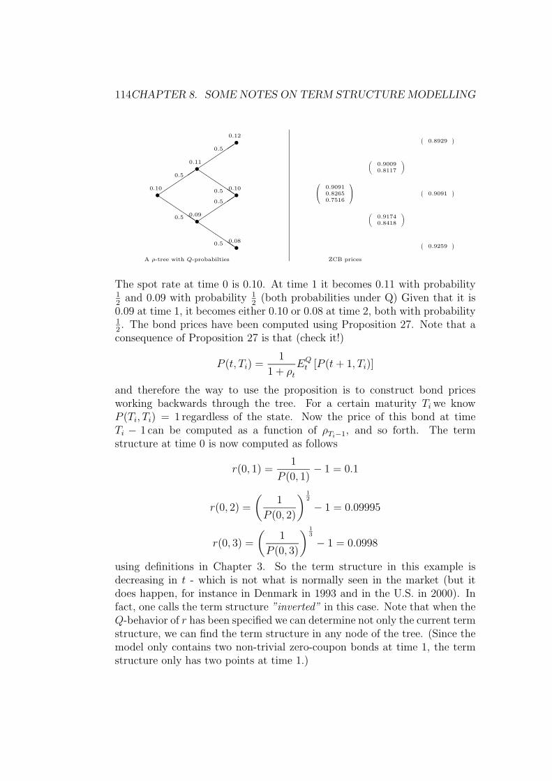
114CHAPTER 8. SOME NOTES ON TERM STRUCTURE MODELLING
s0.100.5
QQQQQ0.5
s0.110.5
QQQQQ0.5
s0.090.5
QQQQQ0.5
s0.12
s0.10
s0.08
A ρ-tree with Q-probabilties
0.90910.82650.7516
(0.90090.8117
)
(0.91740.8418
)
(0.8929
)
(0.9091
)
(0.9259
)ZCB prices
The spot rate at time 0 is 0.10. At time 1 it becomes 0.11 with probability12
and 0.09 with probability 12
(both probabilities under Q) Given that it is0.09 at time 1, it becomes either 0.10 or 0.08 at time 2, both with probability12. The bond prices have been computed using Proposition 27. Note that a
consequence of Proposition 27 is that (check it!)
P (t, Ti) =1
1 + ρtEQt [P (t+ 1, Ti)]
and therefore the way to use the proposition is to construct bond pricesworking backwards through the tree. For a certain maturity Ti we knowP (Ti, Ti) = 1 regardless of the state. Now the price of this bond at timeTi − 1 can be computed as a function of ρTi−1, and so forth. The termstructure at time 0 is now computed as follows
r(0, 1) =1
P (0, 1)− 1 = 0.1
r(0, 2) =
(1
P (0, 2)
) 12
− 1 = 0.09995
r(0, 3) =
(1
P (0, 3)
) 13
− 1 = 0.0998
using definitions in Chapter 3. So the term structure in this example isdecreasing in t - which is not what is normally seen in the market (but itdoes happen, for instance in Denmark in 1993 and in the U.S. in 2000). Infact, one calls the term structure ”inverted” in this case. Note that when theQ-behavior of r has been specified we can determine not only the current termstructure, we can find the term structure in any node of the tree. (Since themodel only contains two non-trivial zero-coupon bonds at time 1, the termstructure only has two points at time 1.)
8.2. CONSTRUCTING AN ARBITRAGE FREE MODEL 115
So Example 10 shows how the term structure is calculated from a Q-treeof the short rate. But what we (or: practitioners) are really interested inis the reverse question: Given todays (observed) term structure, how do weconstruct a Q-tree of the short rate that is consistent with the term structure?(By consistent we mean that if we use the tree for ρ in Example 10-fashion wematch the observed term structure at the first node.) Such a tree is neededfor pricing more complicated contracts (options, for instance).
First, it is easy to see that generally such an “inversion” is in no wayunique; a wide variety of ρ-trees give the same term structure. But that isnot bad; it means that we impose a convenient structure on the ρ-processand still fit observed term structures. Two such conveniences are that thedevelopment of ρ can be represented in a recombining tree (a lattice), or inother words that ρ is Markovian, and that the Q-probability 1/2 is attachedto all branches. (It may not be totally clear that we can do that, but it iseasily seen from the next example/subsection.)
8.2.1 Constructing a Q-tree for the short rate that fitsthe initial term structure
Imagine a situation where two things have been thrust upon us.
1. The almighty (“God “or “The Market”) has determined todays termstructure,
(P (0, 1), P (0, 2), . . . , P (0, T )).
2. Our not-so-almighty boss has difficulties understanding probability be-yond the tossing of a fair coin and wants answers fast, so he(s secretary)has drawn the ρ-lattice in Figure 8.1.
All we have to do is “fill in the blanks’. Optimistically we start, and inthe box corresponding to (t = 0, i = 0) we have no choice but to put
ρ0(0) =1
P (0, 1)− 1.
To fill out boxes corresponding to (t = 1, i = 0) and (t = 1, i = 1) we havethe equation
P (0, 2) =1
ρ0(0)
(1
2× 1
1 + ρ1(0)+
1
2× 1
1 + ρ1(1)
), (8.1)
which of course has many solutions. (Even many sensible ones.) So wecan/have to put more structure on the problem. Two very popular ways of
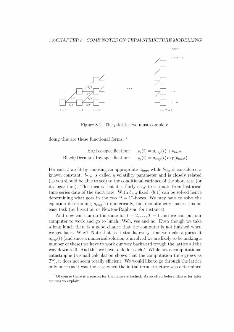
116CHAPTER 8. SOME NOTES ON TERM STRUCTURE MODELLING
1/2
1/2
1/2
1/2
1/2
1/2
. . .
t = 0 t = 1 t = 2 t = T − 1
“level”
i = 0
i = 1
i = T − 1
Figure 8.1: The ρ-lattice we must complete.
doing this are these functional forms: 1
Ho/Lee-specification: ρt(i) = aimp(t) + bhisti
Black/Derman/Toy-specification: ρt(i) = aimp(t) exp(bhisti)
For each t we fit by choosing an appropriate aimp, while bhist is considered aknown constant. bhist is called a volatility parameter and is closely related(as you should be able to see) to the conditional variance of the short rate (orits logarithm). This means that it is fairly easy to estimate from historicaltime series data of the short rate. With bhist fixed, (8.1) can be solved hencedetermining what goes in the two “t = 1”-boxes. We may have to solve theequation determining aimp(1) numerically, but monotonicity makes this aneasy task (by bisection or Newton-Raphson, for instance).
And now can can do the same for t = 2, . . . , T − 1 and we can put ourcomputer to work and go to lunch. Well, yes and no. Even though we takea long lunch there is a good chance that the computer is not finished whenwe get back. Why? Note that as it stands, every time we make a guess ataimp(t) (and since a numerical solution is involved we are likely to be making anumber of these) we have to work our way backward trough the lattice all theway down to 0. And this we have to do for each t. While not a computationalcatastrophe (a small calculation shows that the computation time grows asT 3), it does not seem totally efficient. We would like to go through the latticeonly once (as it was the case when the initial term structure was determined
1Of course there is a reason for the names attached. As so often before, this is for latercourses to explain.
8.2. CONSTRUCTING AN ARBITRAGE FREE MODEL 117
from a known ρ-lattice). Fortunately there is a way of doing this. We needthe following lemma.
Lemma 28 Consider the binomial ρ-lattice in Figure 8.1. Let ψ(t, i) be theprice at time 0 of a security that pays 1 at time t if state/level i occurs atthat time. Then ψ(0, 0) = 1, ψ(0, i) = 0 for i > 0 and the following forwardequation holds:
ψ(t+ 1, i) =
ψ(t,i)
2(1+ρt(i))+ ψ(t,i−1)
2(1+ρt(i−1))0 < i < t+ 1,
ψ(t,i−1)2(1+ρt(i−1))
i = t+ 1,ψ(t,i)
2(1+ρt(i))i = 0.
Proof. We do the proof only for the “0 < i < t + 1”-case, the others aresimilar. Recall that we can think of Ft-measurable random variables (of thetype considered here) as vectors in in Rt+1. Since conditional expectationis linear, we can (for s ≤ t) think of the Fs-conditional expectation of anFt-measurable random variable as a linear mapping from R
t+1 to Rs+1. Inother words it can be represented by a (s+ 1)× (t+ 1)-matrix. In particularthe time t− 1 price of a contract with time t price X can be represented as
EQt
(X
1 + ρt−1
)= Πt−1X
Now note that in the binomial model there are only two places to go from agiven point, so the Πt−1-matrices have the form
Πt−1 =
1−q
1+ρt−1(0)q
1+ρt−1(0)0
1−q1+ρt−1(1)
q1+ρt−1(1)
. . . . . .
0 1−q1+ρt−1(t−1)
q1+ρt−1(t−1)
︸ ︷︷ ︸
t+1 columns
t rows
Let ei(t) be the i’th vector of the standard base in Rt. The claim that pays1 in state i at time t+ 1 can be represented in the lattice by ei+1(t+ 2) andby iterated expectations we have
ψ(t+ 1, i) = Π0Π1 · · ·Πt−1Πtei+1(t+ 2).
But we know that multiplying a matrix by ei(t) from the right picks out thei’th column. For 0 < i < t + 1 we may write the i + 1’st column of Πt as(look at i = 1)
1− q1 + ρt(i− 1)
ei(t+ 1) +q
1 + ρt(i)ei+1(t+ 1).
118CHAPTER 8. SOME NOTES ON TERM STRUCTURE MODELLING
Hence we get
ψ(t+ 1, i) = Π0Π1 · · ·Πt−1
(1− q
1 + ρt(i− 1)ei(t+ 1) +
q
1 + ρt(i)ei+1(t+ 1)
)=
1− q1 + ρt(i− 1)
Π0Π1 · · ·Πt−1ei(t+ 1)︸ ︷︷ ︸ψ(t,i−1)
+q
1 + ρt(i)Π0Π1 · · ·Πt−1ei+1(t+ 1)︸ ︷︷ ︸
ψ(t,i)
,
and since q = 1/2, this ends the proof.
Since P (0, t) =∑t
i=0 ψ(t, i), we can use the following algorithm to fit theinitial term structure.
1. Let ψ(0, 0) = 1 and put t = 1.
2. Let λt(aimp(t − 1)) =∑t
i=0 ψ(t, i) where ψ(t, i) is calculated from theψ(t−1, ·)’s using the specified aimp(t−1)-value in the forward equationfrom Lemma 28.Solve λt(aimp(t− 1)) = P (0, t) numerically for aimp(t− 1).
3. Increase t by one. If t ≤ T then go to 2., otherwise stop.
An inspection reveals that the computation time of this procedure onlygrows as T 2, so we have “gained an order”, which can be quite significantwhen T is large. And don’t worry: There will be exercises to help youunderstand and implement this algorithm.
8.3 On the impossibility of flat shifts of flat
term structures
Now let us demonstrate that in our term structure modelling framework itis impossible to have only parallel shifts of a flat term structure. In otherwords, in a model with no arbitrage we cannot have bond prices at time 0given as
P (0, t) =1
(1 + r)t
for some r ≥ 0, t = 1, . . . , T and
P (1, t) =1
(1 + r)t−1 , t = 2, . . . , T,

8.3. ON THE IMPOSSIBILITY OF FLAT SHIFTS OF FLAT TERM STRUCTURES119
where r is a random variable (which takes on at least two different valueswith positive probability). To assign meaning to a ”flat term structure” attime 1 we should have T ≥ 3.
Now consider the zero-coupon bonds with maturity dates 2 and 3. If theterm structure is flat at time 0 we have for some r ≥ 0
P (0, 2) =1
(1 + r)2 and P (0, 3) =1
(1 + r)3
and if it remains flat at time 1, there exist a random variable r such that
P (1, 2) =1
1 + rand P (1, 3) =
1
(1 + r)2 .
Furthermore, in an arbitrage-free model it will be the case that
P (0, 2) =1
1 + rEQ [P (1, 2)]
=1
1 + rEQ
[1
1 + r
]and
P (0, 3) =1
1 + rEQ [P (1, 3)]
=1
1 + rEQ
[1
(1 + r)2
]Combining these results, we have
1
1 + r= EQ
[1
(1 + r)
]and
1
(1 + r)2 = EQ
[1
(1 + r)2
]which contradicts Jensen’s inequality, for if
1
1 + r= EQ
[1
(1 + r)
]then since u 7−→ u2 is strictly convex and r not constant we must have
1
(1 + r)2 < EQ
[1
(1 + r)2
].
120CHAPTER 8. SOME NOTES ON TERM STRUCTURE MODELLING
Note that the result does not say that it is impossible for the term structure tobe flat. But it is inconsistent with no arbitrage to have a flat term structureand only have the possibility of moves to other flat term structures.
This explains what goes “wrong” in the example in Section 3.5.3. Therethe term structure was flat. We then created a position that had a value of0 at that level of interest rates, but a strictly positive value with at flat termstructure at any other level. But if interest rates are really stochastic thenan arbitrage-free model cannot have only flat shifts of flat structure.
8.4 On forwards and futures
A forward and a futures contract are very similar contracts: The buyer(seller) of either type of contract is obligated to buy (sell) a certain assetat some specified date in the future for a price - the delivery price - agreedupon today. The forward/futures price of a certain asset is the delivery pricewhich makes the forward/futures contract have zero value initially. It is veryimportant to see that a forward/futures price is closer in spirit to the exerciseprice of an option than to the price of an option contract. Whereas an optionalways has positive value (and usually strictly positive) initially, both futuresand forwards have zero value initially because the delivery price is used as abalancing tool.
The following example might clarify this: If a stock trades at $100 todayand we were to consider buying a futures contract on the stock with deliveryin three months and if we had an idea that this stock would not move alot over the next three months, then we would be happy to pay somethingfor a contract which obligated us to buy the stock in three months for, say,$50. Even though things could go wrong and the stock fall below $50 inthree months we consider that a much smaller risk of loss than the chance ofgaining a lot from the contract. Similarly, we would not obligate ourselvesto buying the stock in three months for, say, $150 without receiving somemoney now. Somewhere in between $50 and $150 is a delivery price at whichwe would neither pay nor insist on receiving money to enter into the contract.
In a market with many potential buyers and sellers there is an equilib-rium price at which supply meets demand: The number of contracts withthat delivery price offered at zero initial cost equals the number of contractsdemanded. This equilibrium price is the forward/futures price (dependingon which contract we consider). In the following we will look at this defini-tion in a more mathematical way and we will explain in what sense futuresand forwards are different. Although they produce different cash flows (seebelow) that only results in a price difference when interest rates are stochas-
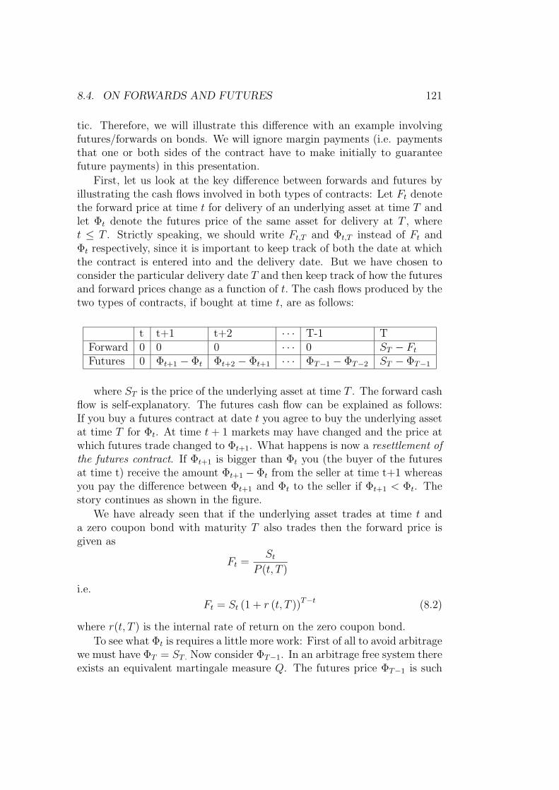
8.4. ON FORWARDS AND FUTURES 121
tic. Therefore, we will illustrate this difference with an example involvingfutures/forwards on bonds. We will ignore margin payments (i.e. paymentsthat one or both sides of the contract have to make initially to guaranteefuture payments) in this presentation.
First, let us look at the key difference between forwards and futures byillustrating the cash flows involved in both types of contracts: Let Ft denotethe forward price at time t for delivery of an underlying asset at time T andlet Φt denote the futures price of the same asset for delivery at T , wheret ≤ T . Strictly speaking, we should write Ft,T and Φt,T instead of Ft andΦt respectively, since it is important to keep track of both the date at whichthe contract is entered into and the delivery date. But we have chosen toconsider the particular delivery date T and then keep track of how the futuresand forward prices change as a function of t. The cash flows produced by thetwo types of contracts, if bought at time t, are as follows:
t t+1 t+2 · · · T-1 TForward 0 0 0 · · · 0 ST − FtFutures 0 Φt+1 − Φt Φt+2 − Φt+1 · · · ΦT−1 − ΦT−2 ST − ΦT−1
where ST is the price of the underlying asset at time T . The forward cashflow is self-explanatory. The futures cash flow can be explained as follows:If you buy a futures contract at date t you agree to buy the underlying assetat time T for Φt. At time t+ 1 markets may have changed and the price atwhich futures trade changed to Φt+1. What happens is now a resettlement ofthe futures contract. If Φt+1 is bigger than Φt you (the buyer of the futuresat time t) receive the amount Φt+1 −Φt from the seller at time t+1 whereasyou pay the difference between Φt+1 and Φt to the seller if Φt+1 < Φt. Thestory continues as shown in the figure.
We have already seen that if the underlying asset trades at time t anda zero coupon bond with maturity T also trades then the forward price isgiven as
Ft =St
P (t, T )
i.e.
Ft = St (1 + r (t, T ))T−t (8.2)
where r(t, T ) is the internal rate of return on the zero coupon bond.
To see what Φt is requires a little more work: First of all to avoid arbitragewe must have ΦT = ST . Now consider ΦT−1. In an arbitrage free system thereexists an equivalent martingale measure Q. The futures price ΦT−1 is such
122CHAPTER 8. SOME NOTES ON TERM STRUCTURE MODELLING
that the cash flow promised by the contract (bought at T − 1) has value 0.We must therefore have
0 = EQT−1
[ST − ΦT−1
RT−1,T
]but since RT−1,T is FT−1-measurable this implies
0 =1
RT−1,T
EQT−1 [ST − ΦT−1]
i.e.ΦT−1 = EQ
T−1 [ST ] (8.3)
Since Q is a martingale measure recall that
ST−1
R0,T−1
= EQT−1
[STR0,T
]i.e.
ST−1 =1
1 + ρT−1
EQT−1 [ST ]
hence we can write (8.3) as
ΦT−1 =(1 + ρT−1
)ST−1
and that is the same as (8.2) since the yield on a one period zero coupon bondis precisely the spot rate. So we note that with one time period remainingwe have ΦT−1 = FT−1. But that also follows trivially since with one periodremaining the difference in cash flows between forwards and futures does nothave time to materialize.
Now consider ΦT−2. By definition ΦT−2 should be set such that the cashflow of the futures contract signed at T − 2 has zero value:
0 = EQT−2
[ΦT−1 − ΦT−2
RT−2,T−1
+ST − ΦT−1
RT−2,T
](8.4)
Now note that using the rule of iterated expectations and the expression forΦT−1 we find
EQT−2
[ST − ΦT−1
RT−2,T
]=
1
RT−2,T−1
EQT−2
[EQT−1
[ST − ΦT−1
RT−1,T
]]= 0
8.4. ON FORWARDS AND FUTURES 123
so (8.4) holds precisely when
0 = EQT−2
[ΦT−1 − ΦT−2
RT−2,T−1
]=
1
RT−2,T−1
EQT−2 [ΦT−1 − ΦT−2]
i.e. we haveΦT−2 = EQ
T−2 [ΦT−1] = EQT−2 [ST ] .
This argument can be continued backwards and we arrive at the expression
Φt = EQt [ST ] (8.5)
Note that (8.5) is not in general equal to (8.2):
Under Q, we have St = EQt
[STRt,T
]so if 1
Rt,Tand ST are uncorrelated under
Q we may write
St = EQt
[1
Rt,T
]EQt [ST ] = P (t, T )Φt
which would imply that
Φt =St
P (t, T )= Ft
Hence, if 1Rt,T
and ST are uncorrelated under Q, the forward price Ftand the futures price Φt are the same. A special case of this is when interestrates are deterministic, i.e. all future spot rates and hence Rt,T are known attime t.
Note that in general,
Φt − Ft =1
P (t, T )
(P (t, T )EQ
t [ST ]− St)
=1
P (t, T )
(EQt
[1
Rt,T
]EQt [ST ]− St
)=
1
P (t, T )
(EQt
(STRt,T
)− CovQt
(1
Rt,T
, ST
)− St
)=
−1
P (t, T )
(CovQt
(1
Rt,T
, ST
)).
Note that margin payments go to the holder of a futures contract whenspot prices rise, i.e. in states where ST is high. If 1
R(t,T )is negatively correlated
with ST , then interest rates tend to be high when the spot price is high andhence the holder of a futures contract will receive cash when interest ratesare high. Hence a futures contract is more valuable in that case and thefutures price should therefore be set higher to keep the contract value at 0.

124CHAPTER 8. SOME NOTES ON TERM STRUCTURE MODELLING
8.5 On swap contracts
A swap contract is an agreement to exchange one stream of payments foranother. A wide variety of swaps exists in financial markets; they are of-ten tailor-made to the specific need of a company/an investor and can behighly complex. However, we consider only the valuation of the simplest2
interest rate swap where fixed interest payments are exchanged for floatingrate interest payments.
This swap you may see referred to as anything from “basis” to “forwardstarting ???monthly payer swap settled in arrears”. Fortunately the pay-ments are easier to describe. For a set of equidistant dates (Ti)
ni=0, say δ
apart, it is a contract with cash flow (per unit of notational principal) 1
P (Ti−1, Ti)− 1︸ ︷︷ ︸
floating leg
− δκ︸︷︷︸fixed leg
at date Ti for i = 1, . . . , n,
where κ is a constant (an interest rate with δ-compounding quoted on yearlybasis.) You should convince yourself why the so-called floating leg doesin fact correspond to receiving floating interest rate payments. The term(1/P (Ti−1, Ti) − 1)/δ is often called the (12*δ)-month LIBOR (which anacronym for London Interbank Offer Rate, and does not really mean anythingnowadays, it is just easy to pronounce). Note that the payment made at Tiis known at Ti−1.
It is clear that since the payments in the fixed leg are deterministic, theyhave a value of
δκn∑i=1
P (t, Ti).
The payments in the floating leg are not deterministic. But despite this,we can find their value without a stochastic model for bond prices/interestrates. Consider the following simple portfolio strategy:
Time Action Net cash flowt Sell 1 Ti-ZCB
Buy 1 Ti−1-ZCB P (t, Ti)− P (t, Ti−1)Ti−1 Use principal received from Ti−1-ZCB
to buy 1/P (Ti−1, Ti) Ti-ZCBs 0Ti Close position 1/P (Ti−1, Ti)− 1
2Simple objects are often referred to as plain vanilla objects. But what is seen as simpledepends very much on who is looking.
8.5. ON SWAP CONTRACTS 125
This means that the Ti-payment in the floating leg has a value of P (t, Ti−1)−P (t, Ti), so when summing over i see that the value of the floating leg is
P (t, T0)− P (t, Tn).
In the case where t = T0 this is easy to remember/interpret. A bullet-likebond that has a principal of 1 pays a coupon that is the short rate musthave a price of 1 (lingo: “it is trading at par”). The only difference betweenthis contract and the floating leg is the payment of the principal at timeTn; the time t value of this is P (t, Tn) hence the value of the floating leg is1− P (t, Tn).
All in all the swap has a value of
V = P (t, T0)− P (t, Tn)− δκn∑i=1
P (t, Ti)).
But there is a further twist; these basis swaps are only traded with one κ(for each length; each n), namely the one that makes the value 0. This rateis called the swap rate (at a given date for a given maturity)
κn(t) =P (t, T0)− P (t, Tn)
δ∑n
i=1 P (t, Ti). (8.6)
In practice (8.6) is often used “backwards”, meaning that swap rates forswaps of different lengths (called the “swap curve”) are used to infer discountfactors/the term structure. Note that this is easy to do recursively if we can“get started”, which is clearly the case if t = T0.3
The main point is that the basis swap can be priced without using afull dynamic model, we only need today’s term structure. But it takes onlyminor changes in the contract specification for this conclusion to break down.For instance different dynamic models with same current term structure givedifferent swap values if the ith payment in the basis swap is transferred todate Ti−1 (where it is first known; this is called settlement in advance) or ifwe swap every 3 months against the 6-month LIBOR.
The need for a swap-market can also be motivated by the following exam-ple showing swaps can offer comparative advantages. In its swap-formulationit is very inspired by Hull’s book, but you you should recognize the idea fromintroductory economics courses (or David Ricardo’s work of 1817, whichevercame first). Consider two firms, A and B, each of which wants to borrow
3There should be a “don’t try this at work” disclaimer here. In the market differentday count conventions are often used on the two swap legs, so things may not be quitewhat they seem.
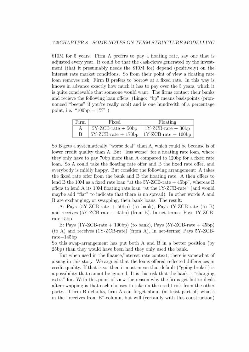
126CHAPTER 8. SOME NOTES ON TERM STRUCTURE MODELLING
$10M for 5 years. Firm A prefers to pay a floating rate, say one that isadjusted every year. It could be that the cash-flows generated by the invest-ment (that it presumably needs the $10M for) depend (positively) on theinterest rate market conditions. So from their point of view a floating rateloan removes risk. Firm B prefers to borrow at a fixed rate. In this way isknows in advance exactly how much it has to pay over the 5 years, which itis quite concievable that someone would want. The firms contact their banksand recieve the following loan offers: (Lingo: “bp” means basispoints (pron-uonced “beeps” if you’re really cool) and is one hundredth of a percentagepoint, i.e. “100bp = 1%” )
Firm Fixed FloatingA 5Y-ZCB-rate + 50bp 1Y-ZCB-rate + 30bpB 5Y-ZCB-rate + 170bp 1Y-ZCB-rate + 100bp
So B gets a systematically “worse deal” than A, which could be because is oflower credit quality than A. But “less worse” for a floating rate loan, wherethey only have to pay 70bp more than A compared to 120bp for a fixed rateloan. So A could take the floating rate offer and B the fixed rate offer, andeverybody is mildly happy. But consider the following arrangement: A takesthe fixed rate offer from the bank and B the floating rate. A then offers tolend B the 10M as a fixed rate loan “at the 5Y-ZCB-rate + 45bp”, whereas Boffers to lend A its 10M floating rate loan “at the 1Y-ZCB-rate” (and wouldmaybe add “flat” to indicate that there is no spread). In other words A andB are exchanging, or swapping, their bank loans. The result:
A: Pays (5Y-ZCB-rate + 50bp) (to bank), Pays 1Y-ZCB-rate (to B)and receives (5Y-ZCB-rate + 45bp) (from B). In net-terms: Pays 1Y-ZCB-rate+5bp
B: Pays (1Y-ZCB-rate + 100bp) (to bank), Pays (5Y-ZCB-rate + 45bp)(to A) and receives (1Y-ZCB-rate) (from A). In net-terms: Pays 5Y-ZCB-rate+145bpSo this swap-arrangement has put both A and B in a better position (by25bp) than they would have been had they only used the bank.
But when used in the finance/interest rate context, there is somewhat ofa snag in this story. We argued that the loans offered reflected differences incredit quality. If that is so, then it must mean that default (“going broke”) isa possibility that cannot be ignored. It is this risk that the bank is “chargingextra” for. With this point of view the reason why the firms get better dealsafter swapping is that each chooses to take on the credit risk from the otherparty. If firm B defaults, firm A can forget about (at least part of) what’sin the “receives from B”-column, but will (certainly with this construction)
8.6. ON EXPECTATION HYPOTHESES 127
only be able to get out of its obligations to B to a much lesser extent. Sothe firms are getting lower rates by taking on default risk, which a risk ofthe type “a large loss with a small probability”. One can quite sensibly askif that is the kind of risks that individual firms want to take.
One could try to remedy the problem by saying that we set up a financialinstitution through which the swapping takes place. This institution shouldensure payments to the non-defaulting party (hence taking “credit risk” ×2), in return for a share of the possible “lower rate”-gain from the swap, andhope for some “law of large numbers”-diversification effect. But that storyis questionable; isn’t that what the bank is doing in the first place?
So the morale is two-fold: i) If something seems to be too good to be trueit usually is. Also in credit risk models. ii) The only way to see if the spreadsoffered to firms A and B are set such that there is no gain without extra risk,i.e. consistent with no arbitrage, is to set up a real dynamic stochastic modelof the defaults (something that subsequent courses will do), just as stochasticterm structure models help us realize that non-flat yield curves do not implyarbitrage.
8.6 On expectation hypotheses
Recall that the spot rate in our term structure models is a stochastic pro-cess. At time 0 we do not know what the spot rate will be at time 1.Wemay however from current bond prices compute the one-period forward ratef(1, 2) and it is natural to think that this rate at least carries some infor-mation about the level of the spot rate at time 1.For example, one type ofexpectation hypothesis would argue, that the expected value of spot rates isequal to the corresponding forward rates. As we shall see shortly, there islittle reason to think that this is satisfied in arbitrage-free models. There area number of other expectation hypotheses that one can formulate concerningfuture levels of interest rates, bond prices, yields and forward rates. Althoughwe will no go through all of these in great detail, one point should be clearafter this: There is essentially only one expectation hypothesis which followsas a simple consequence of no arbitrage (and an assumption of risk neutralagents). Many other form of expectation hypothesis have little mathematicaljustification, often there are inconsistent with each other, and very often thesame form of the expectation hypotheses cannot hold for different maturities.
But let us begin with the good news. We know that in an arbitrage-freemodel, we have for any zero coupon bond with maturity Ti that
P (t, Ti) =1
1 + ρtEQt [P (t+ 1, Ti)] .
128CHAPTER 8. SOME NOTES ON TERM STRUCTURE MODELLING
Hence standing at time t, the expected return under Q of holding a bond inone period is
EQt [P (t+ 1, Ti)]
P (t, Ti)− 1 = ρt
and this does not depend on the maturity of the bond. Hence under Q, theone-period return on all bonds is the same. This is a mathematical conse-quence of no arbitrage. It becomes a hypothesis, which we may call the localexpectations hypothesis, once we claim that this also holds under the measureP which governs the evolution of interest rates in the real world. This wouldof course be true if P = Q, something which only holds in an economy inwhich all agents are risk-neutral.
Let us assume that P = Q and consider an extension (called the “returnto maturity hypothesis”) of this local hypothesis to n periods which equatesthe expected return from rolling over the money market account in n periodswith that of holding an n−period bond. This would be equivalent to statingthat
EQt (Rt,t+n) = (1 + y(t, t+ n))n
where y(t, t+n) is the yield at time t of a bond maturing at time t+n. Whatif we claim that this holds for all n? Then Jensen’s inequality brings us intotrouble since from our fundamental pricing relationship we have
P (t, t+ n) =
1
(1 + y(t, t+ n))n= EQ
t
[1
Rt,t+n
]and unless interest rates are deterministic we have
EQt
[1
Rt,t+n
]>
1
EQt Rt,t+n
.
Finally let us consider another popular hypothesis about the term struc-ture of interest rates, which states that forward rates are unbiased predictorsof spot rates. Our discussion of this hypothesis will be much clearer if wehave at our disposal the concept of forward measures.
Proposition 29 Given a term structure model with Q as the martingalemeasure. Define the random variable ZT
T as
ZTT =
1
R0,T+1P (0, T + 1).
8.6. ON EXPECTATION HYPOTHESES 129
Then a new probability measure QT is defined by letting
QT (A) = EQ(ZTT 1A
), A ∈ F . (8.7)
Under this measure, the forward rate process (f(t, T ))t=0,...,T is a martingale.Proof. First note that since ρ > −1, ZT
T > 0.Also,
EQ(ZTT
)=
1
P (0, T + 1)EQ 1
R0,T+1
= 1
and therefore (8.7) defines a new probability measure on Ω. Let
ZTt = EQ
t
(ZTT
)=
1
R(0, t)P (0, T + 1)EQt
(1
Rt,T+1
)=
P (t, T + 1)
R(0, t)P (0, T + 1).
Now note that
EQt
(ρT
Rt,T+1
)= P (0, T + 1)R0,tE
Qt
(ρT
R0,T+1P (0, T + 1)
)=
P (t, T + 1)
ZTt
EQt
(ZTT ρT
)= P (t, T + 1)EQT
t (ρT ) .
Therefore,
EQT
t (ρT ) =1
P (t, T + 1)EQt
(ρT
Rt,T+1
)=
1
P (t, T + 1)EQt
(1 + ρTRt,T+1
− 1
Rt,T+1
)=
1
P (t, T + 1)EQt
(1
Rt,T
− 1
Rt,T+1
)=
P (t, T )
P (t, T + 1)− 1
= f(t, T ).
This proves the martingale property.This proposition shows that there exists a measure (and this measure
is called the T−forward measure) under which the expected spot rate at

130CHAPTER 8. SOME NOTES ON TERM STRUCTURE MODELLING
time T is equal to the forward rate. Typically, the forward measure is notequal to P , and it is not equal to Q unless interest rates are deterministic.Furthermore, one may check that for f(t, T ) and f(t, T + 1) to be unbiasedestimators of rT and rT+1,respectively, the spot interest rate at time T mustbe deterministic. The moral of all this, is that viewing the forward rate asunbiased estimators of future spot rates is problematic.
8.7 Why P = Q means risk neutrality
In this section we will keep referring to the measure P which is the measuredetermining the actual evolution of prices. To make sure that the meaningof P is clear, we can say that a statistician estimating parameters of prices istrying to find P. We have seen that the version of the expectations hypoth-esis known as the local expectations hypothesis holds under the martingalemeasure Q used for pricing. Recall that the measure Q is a measure whichallows us to give convenient expressions for prices of claims and derivativesecurities but not a measure governing the actual movement of prices.
We have stated earlier somewhat loosely that P and Q are actually thesame when agents are risk neutral. Since we have not seen many agents thisstatement needs some elaboration. A quick sketch of this line of reasoningis the following: Recall that under Q all securities have the same one periodreturns: They are equal to the short rate. If Q = P it would be the casethat actual expected returns were the same for all assets, regardless of theirvariances. This would only be possible in a world where agents are riskneutral and therefore do not care about risk (variance, say) but look only atexpected returns and prefer more expected return to less. In fact, if thereis as much as one risk neutral agent in the economy and two assets havedifferent expected returns, then this one agent would ruin the equilibrium bydemanding infinitely much of the asset with the high expected return andfinancing the purchase by selling the asset with low expected return in infinitequantities. Therefore, we may say that Q = P follows from risk neutralityof at least one agent. The argument can be made more precise by explicitlymodelling the inter-temporal optimization problem of a representative agentwho maximizes an additively separable expected utility of consumption overa certain time period. When this is done we can interpret the pricing relation
P (t, Ti) =1
1 + ρtEQt [P (t+ 1, Ti)]
in terms of marginal utilities. The key result is that in equilibrium the pricesof bonds adjust in such a way that the increase in marginal utility for the
8.7. WHY P = Q MEANS RISK NEUTRALITY 131
agent obtained by selling the bond at date t and using the proceeds forconsumption is exactly equal to the marginal loss of expected utility at datet+ 1 resulting from the smaller amount of money for consumption availableby selling the position in that bond at time t+1. Let us consider a one-periodcase. If we denote by C0 (known at time 0) and C1 (stochastic viewed fromtime 0) the optimal consumption of the agent at dates 0 and 1, it will be thecase in equilibrium that the price of the i′th asset satisfies
P i(0)u′(C0) = EP0
[P i(1)u′(C1)
]i.e.
P i(0) = EP0
[P i(1)u′(C1)
u′(C0)
]= EP
t
[P i(1)Z1
1 + ρ0
]where
Z1 =u′(C1)
EP0 u′(C1)
1 + ρ0 =u′(C0)
EPt u′(C1)
and this we may then write as
P i(0) = EQt
[P i(1)
1 + ρ0
]where Q is defined by
Q(A) = EP (1AZ1).
This establishes the connection between utility maximization and the equiv-alent martingale measure. An agent who is risk neutral will have an affineutility function, and hence for such an agent u′(C1) is constant (i.e. does notvary with ω as C1 does). In that case Z1 = 1 and P = Q.
It is clear that P = Q is sufficient for the local expectation hypothesis tohold but it may seem to be too strong a requirement. After all, it is only anexpectation of one random variable that we are referring to and one couldimagine that a measure change would not alter this particular expectation.To analyze this question a little further, consider the fundamental definitionof a new measure through the random variable Z1 :
Q(A) = EP (1AZ1).
132CHAPTER 8. SOME NOTES ON TERM STRUCTURE MODELLING
For some random variable X,which could be the spot rate at some futuredate, we have
EQ(X) = EP (XZ)
and therefore EQ(X) = EP (X) if and only if
EP (X(Z − 1)) = 0.
Since E(Z − 1) = 0 this is the same as requiring
Cov(X,Z) = 0.
Therefore, for the change of measure to preserve a mean value we must havethat the variable in question is uncorrelated with the change of measurevariable Z, and this will typically not hold in the term structure models weconsider.
Chapter 9
Portfolio Theory
Matrix Algebra
First we need a few things about matrices. (A very useful reference for math-ematical results in the large class imprecisely defined as “well-known”is Berck& Sydsæter (1992), “Economists’ Mathematical Handbook”, Springer.)
• When x ∈ Rn and V ∈ Rn×n then
∂
∂x(x>Vx) = (V + V>)x
• A matrix V ∈ Rn×n is said to be positive definite if z>Vz > 0 for allz 6= 0. If V is positive definite then V−1 exists and is also positivedefinite.
• Multiplying (appropriately) partitioned matrices is just like multiplying2× 2-matrices.
• When X is an n-dimensional random variable with covariance matrixΣ then
Cov(AX + B,CX + D) = AΣC>,
where A, B, C, and D are deterministic matrices such that the multi-plications involved are well-defined.
Basic Definitions & Justification of Mean-Variance Analysis
We will consider an agent who wants to invest in the financial markets. Welook at a simple model with only two time-points, 0 and 1. The agent hasan initial wealth of W0 to invest. We are not interested in how the agent
133
134 CHAPTER 9. PORTFOLIO THEORY
determined this amount, it’s just there. There are n financial assets to choosefrom and these have prices
Si,t for i = 1, . . . , n and t = 0, 1,
where Si,1 is stochastic and not known until time 1. The rate of return onasset i is defined as
ri =Si,1 − Si,0
Si,0,
and r = (r1, . . . , rn)> is the vector of rates of return. Note that r is stochastic.At time 0 the agent chooses a portfolio, that is he buys ai units of asset
i and since all in all W0 is invested we have
W0 =n∑i=1
aiSi,0.
(If ai < 0 the agent is selling some of asset i; in most of our analysis short-selling will be allowed.)
Rather than working with the absolute number of assets held, it is moreconvenient to work with relative portfolio weights. This means that for theith asset we measure the value of the investment in that asset relative tototal investment and call this wi, i.e.
wi =aiSi,0∑ni=1 aiSi,0
=aiSi,0W0
.
We put w = (w1, . . . wn)>, and have that w>1 = 1. In fact, any vectorsatisfying this condition identifies an investment strategy. Hence in the fol-lowing a portfolio is a vector whose coordinate sum to 1. Note that in thisone period model a portfolio w is not a stochastic variable (in the sense ofbeing unknown at time 0).
The terminal wealth is
W1 =n∑i=1
aiSi,1 =n∑i=1
ai(Si,1 − Si,0) +n∑i=1
aiSi,0
= W0
(1 +
n∑i=1
Si,0aiW0
Si,1 − Si,0Si,0
)= W0(1 + w>r), (9.1)
so if we know the relative portfolio weights and the realized rates of return,we know terminal wealth. We also see that
E(W1) = W0(1 + w>E(r))
135
and
Var(W1) = W 20 Cov(w>r,w>r) = W 2
0 w>Var(r)w.
In this chapter we will look at how agents should choose w. We willfocus on how to choose w such that for a given expected rate of return, thevariance on the rate of return is minimized. This is called mean-varianceanalysis. Intuitively, it sounds reasonable enough, but can it be justified?
An agent has a utility function, u, and let us for simplicity say that hederives utility from directly from terminal wealth. (So in fact we are sayingthat we can eat money.) We can expand u in a Taylor series around theexpected terminal wealth,
u(W1) = u(E(W1)) + u′(E(W1))(W1 − E(W1))
+1
2u′′(E(W1))(W1 − E(W1))2 +R3,
where the remainder term R3 is
R3 =∞∑i=3
1
i!u(i)(E(W1))(W1 − E(W1))i,
“and hopefully small”. With appropriate (weak) regularity condition thismeans that expected terminal wealth can be written as
E(u(W1)) = u(E(W1)) +1
2u′′(E(W1))Var(W1) + E(R3),
where the remainder term involves higher order central moments. As usualwe consider agents with increasing, concave (i.e. u′′ < 0) utility functionswho maximize expected wealth. This then shows that to a second orderapproximation there is a preference for expected wealth (and thus, by (9.1),to expected rate of return), and an aversion towards variance of wealth (andthus to variance of rates of return).
But we also see that mean-variance analysis cannot be a completely gen-eral model of portfolio choice. A sensible question to ask is: What restrictionscan we impose (on u and/or on r) to ensure that mean-variance analysis isfully consistent with maximization of expected utility?
An obvious way to do this is to assume that utility is quadratic. Then theremainder term is identically 0. But quadratic utility does not go too wellwith the assumption that utility is increasing and concave. If u is concave(which it has to be for mean-variance analysis to hold ; otherwise our interestwould be in maximizing variance) there will be a point of satiation beyond
136 CHAPTER 9. PORTFOLIO THEORY
which utility decreases. Despite this, quadratic utility is often used with a“happy-go-lucky” assumption that when maximizing, we do not end up inan area where it is decreasing.
We can also justify mean-variance analysis by putting distributional re-strictions on rates of return. If rates of return on individual assets are nor-mally distributed then the rate of return on a portfolio is also normal, andthe higher order moments in the remainder can be expressed in terms of thevariance. In general we are still not sure of the signs and magnitudes ofthe higher order derivatives of u, but for large classes of reasonable utilityfunctions, mean-variance analysis can be formally justified.
9.1 The Mathematics of the Efficient Frontier
9.1.1 The case with no riskfree asset
First we consider a market with no riskfree asset and n risky assets. Laterwe will include a riskfree asset, and it will become apparent that we havedone things in the right order.
The risky assets have a vector of rates of return of r, and we assume that
E(r) = µ, (9.2)
Var(r) = Σ, (9.3)
where Σ is positive definite (hence invertible) and not all coordinates of µare equal. As a covariance matrix Σ is always positive semidefinite, thedefiniteness means that there does not exist an asset whose rate of returncan be written as an affine function of the other n− 1 assets’ rates of return.Note that the existence of a riskfree asset would violate this.
Consider the following problem:
minw1
2w>Σw := σ2
P subject to w>µ = rP
w>1 = 1
First note that our assumptions on µ and Σ ensure that a unique finitesolution exits for any value of rP . Second note that the problem can beinterpreted as choosing portfolio weights (the second constraint ensures thatw is a vector of portfolio weights) such that the variance on the return on theportfolio (w>Σw; the “1/2” is just there for convenience) is minimized giventhat we want a specific expected rate of return (rP ; “P is for portfolio”).
9.1. THE MATHEMATICS OF THE EFFICIENT FRONTIER 137
To solve the problem we set up the Lagrange-function with multipliers
L(w, λ1, λ2) =1
2w>Σw − λ1(w>µ− rP )− λ2(w>1− 1).
The first-order conditions for optimality are
∂L∂w
= Σw − λ1µ− λ21 = 0, (9.4)
w>µ− rP = 0, (9.5)
w>1− 1 = 0. (9.6)
Usually we might say “and these are linear equations that can easily besolved”, but working on them algebraically leads to a much deeper under-standing and intuition about the model. Note that invertibility gives thatwe can write (9.4) as (check for yourself)
w = Σ−1[µ 1]
[λ1
λ2
], (9.7)
and (9.5)-(9.6) as
[µ 1]>w =
[rP1
]. (9.8)
Multiplying both sides of (9.7) by [µ 1]> and using (9.8) gives[rP1
]= [µ 1]>w = [µ 1]>Σ−1[µ 1]︸ ︷︷ ︸
:=A
[λ1
λ2
]. (9.9)
By using the multiplication rules for partitioned matrices we see that
A =
[µ>Σ−1µ µ>Σ−11µ>Σ−11 1>Σ−11
]:=
[a bb c
]We now show that A is positive definite, in particular it is invertible. To thisend let z> = (z1, z2) 6= 0 be an arbitrary non-zero vector in R2. Then
y = [µ 1]
[z1
z2
]= [z1µ z21] 6= 0,
because the coordinates of µ are not all equal. From the definition of A weget
∀z 6= 0 : z>Az = y>Σ−1y > 0,
138 CHAPTER 9. PORTFOLIO THEORY
because Σ−1 is positive definite (because Σ is). In other words, A is positivedefinite. Hence we can solve (9.9) for the λ’s,[
λ1
λ2
]= A−1
[rP1
],
and insert this into (9.7) in order to determine the optimal portfolio weights
w = Σ−1[µ 1]A−1
[rP1
]. (9.10)
The portfolio w is called the minimum variance portfolio for a given mean rP(So we can’t be bothered to say the correct full phrase: “minimum varianceon rate of return for a given mean rate on return rP ”.) Twice the optimalvalue (i.e. the minimal portfolio return variance) is
σ2P = w>Σw
= [rP 1]A−1[µ 1]>Σ−1ΣΣ−1[µ 1]A−1[rP 1]>
= [rP 1]A−1([µ 1]>Σ−1[µ 1]
)︸ ︷︷ ︸=A by def.
A−1[rP 1]>
= [rP 1]A−1
[rP1
],
where symmetry (of Σ and A and their inverses) was used to obtain thesecond line. But note that
A−1 =1
ac− b2
[c −b−b a
],
which gives us
σ2P =
a− 2brP + cr2P
ac− b2. (9.11)
In (9.11) the relation between the variance of the minimum variance portfoliofor a given rp, σ
2P , is expressed as a parabola and is called the variance
portfolio frontier or locus. In mean-standard deviation-space the relationis expressed as a hyperbola. Figure 9.1 illustrates what things look like inmean-variance-space. (When using graphical arguments you should be quitecareful to use “the right space”; for instance lines that are straight in onespace, are not straight in the other.) The upper half of the curve in Figure9.1 (the solid line) identifies the set of portfolios that have the highest meanreturn for a given variance; these are called mean-variance efficient portfolios.The portfolios on the bottom half (the dotted part) are called inefficient
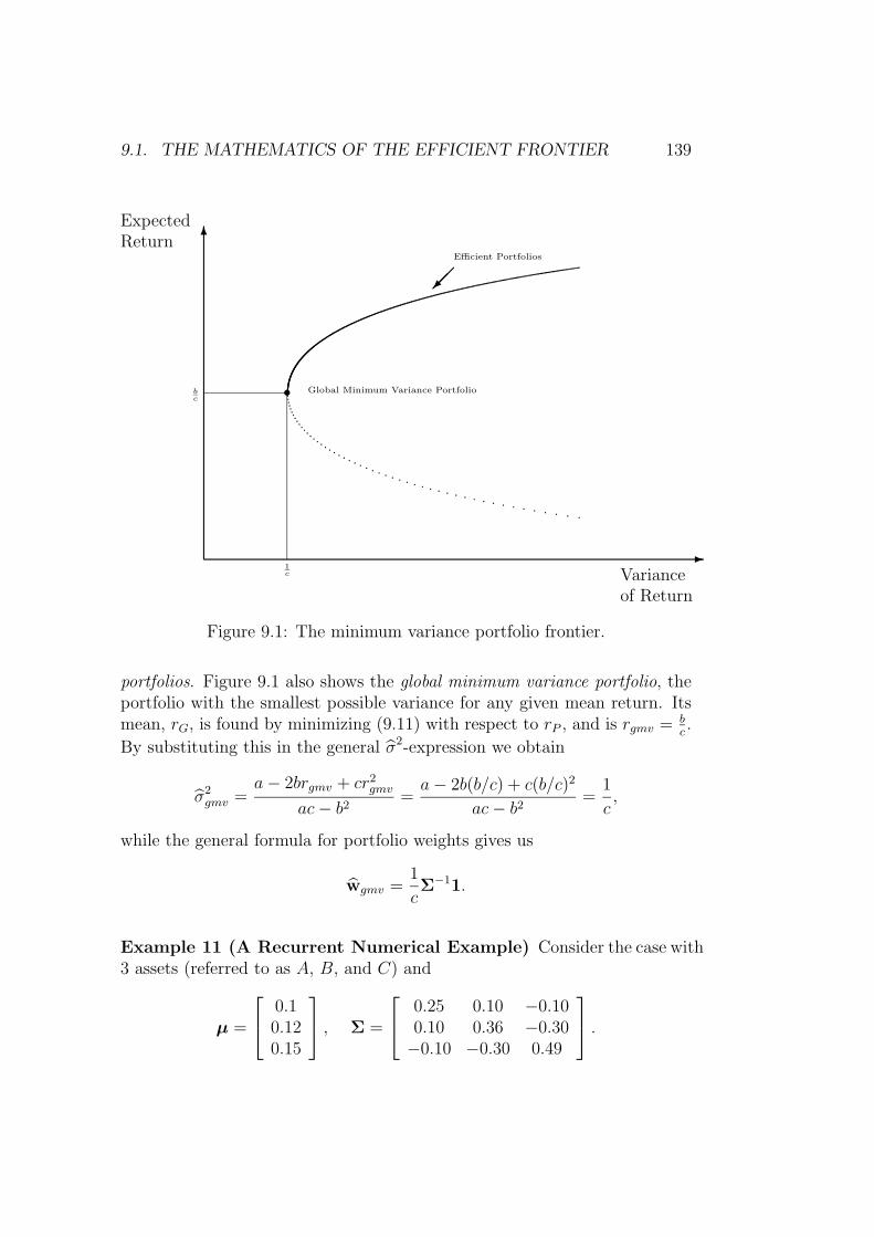
9.1. THE MATHEMATICS OF THE EFFICIENT FRONTIER 139
6
-
ExpectedReturn
Varianceof Return
s Global Minimum Variance Portfolio
Efficient Portfolios
bc
1c
Figure 9.1: The minimum variance portfolio frontier.
portfolios. Figure 9.1 also shows the global minimum variance portfolio, theportfolio with the smallest possible variance for any given mean return. Itsmean, rG, is found by minimizing (9.11) with respect to rP , and is rgmv = b
c.
By substituting this in the general σ2-expression we obtain
σ2gmv =
a− 2brgmv + cr2gmv
ac− b2=a− 2b(b/c) + c(b/c)2
ac− b2=
1
c,
while the general formula for portfolio weights gives us
wgmv =1
cΣ−11.
Example 11 (A Recurrent Numerical Example) Consider the case with3 assets (referred to as A, B, and C) and
µ =
0.10.120.15
, Σ =
0.25 0.10 −0.100.10 0.36 −0.30−0.10 −0.30 0.49
.
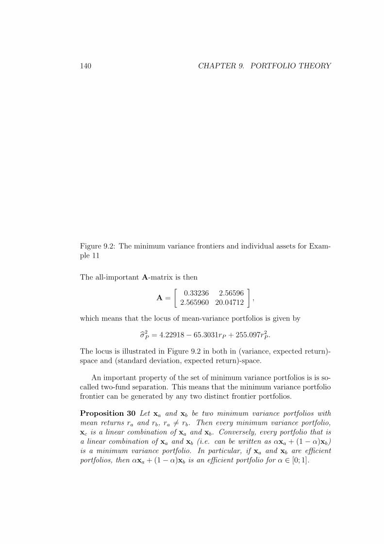
140 CHAPTER 9. PORTFOLIO THEORY
Figure 9.2: The minimum variance frontiers and individual assets for Exam-ple 11
The all-important A-matrix is then
A =
[0.33236 2.56596
2.565960 20.04712
],
which means that the locus of mean-variance portfolios is given by
σ2P = 4.22918− 65.3031rP + 255.097r2
P .
The locus is illustrated in Figure 9.2 in both in (variance, expected return)-space and (standard deviation, expected return)-space.
An important property of the set of minimum variance portfolios is is so-called two-fund separation. This means that the minimum variance portfoliofrontier can be generated by any two distinct frontier portfolios.
Proposition 30 Let xa and xb be two minimum variance portfolios withmean returns ra and rb, ra 6= rb. Then every minimum variance portfolio,xc is a linear combination of xa and xb. Conversely, every portfolio that isa linear combination of xa and xb (i.e. can be written as αxa + (1 − α)xb)is a minimum variance portfolio. In particular, if xa and xb are efficientportfolios, then αxa + (1− α)xb is an efficient portfolio for α ∈ [0; 1].
9.1. THE MATHEMATICS OF THE EFFICIENT FRONTIER 141
Proof. To prove the first part let rc denote the mean return on a givenminimum variance portfolio xc. Now choose α such that rc = αra+(1−α)rb,that is α = (rc − rb)/(ra − rb) (which is well-defined because ra 6= rb). Butsince xc is a minimum variance portfolio we know that (9.10) holds, so
xc = Σ−1[µ 1]A−1
[rc1
]= Σ−1[µ 1]A−1
[αra + (1− α)rbα + (1− α)
]= αxa + (1− α)xb,
where the third line is obtained because xa and xb also fulfill (9.10). Thisproves the first statement. The second statement is proved by “reading fromright to left” in the above equations. This shows that xc = αxa+(1−α)xb isthe minimum variance portfolio with expected return αra + (1− α)rb. Fromthis, the validity of the third statement is clear.
Another important notion is orthogonality of portfolios. We say that twoportfolios xP and xzP (“z is for zero”) are orthogonal if the covariance oftheir rates of return is 0, i.e.
x>zPΣxP = 0. (9.12)
Often xzP is called xP ’s 0-β portfolio (we’ll see why later).
Proposition 31 For every minimum variance portfolio, except the globalminimum variance portfolio, there exists a unique orthogonal minimum vari-ance portfolio. Furthermore, if the first portfolio has mean rate of return rP ,its orthogonal one has mean
rzP =a− brPb− crP
.
Proof. First note that rzP is well-defined for any portfolio except the globalminimum variance portfolio. By (9.10) we know how to find the minimumvariance portfolios with means rP and rzP = (a− brP )/(b− crP ). This leadsto
x>zPΣxP = [rzP 1]A−1[µ 1]>Σ−1ΣΣ−1[µ 1]A−1[rP 1]>
= [rzP 1]A−1([µ 1]>Σ−1[µ 1]
)︸ ︷︷ ︸=A by def.
A−1[rP 1]>

142 CHAPTER 9. PORTFOLIO THEORY
= [rzP 1]A−1
[rP1
](9.13)
=
[a− brPb− crP
1
]1
ac− b2
[c −b−b a
] [rP1
]=
1
ac− b2
[a− brPb− crP
1
] [crP − ba− brP
]= 0,
which was the desired result.
Proposition 32 Let xmv (6= xgmv, the global minimum variance portfolio) bea portfolio on the mean-variance frontier with rate of return rmv, expected rateof return µmv and variance σ2
mv. Let xzmv be the corresponding orthogonalportfolio, xP be an arbitrary portfolio, and use similar notation for rates ofreturn on these portfolios. Then the following holds:
µP − µzmv = βP,mv(µmv − µzmv),
where
βP,mv =Cov(rP , rmv)
σ2mv
.
Proof. Consider first the covariance between return on asset i and xmv. Byusing (9.10) we get
Cov(ri, rmv) = e>i Σxmv
= e>i [µ 1]A−1
[µmv
1
]= [µi 1]A−1
[µmv
1
].
From calculations in the proof of Proposition 31 we know that the covari-ance between xmv and xzvp is given by (9.13). We also know that it is 0.Subtracting this 0 from the above equation gives
Cov(ri, rmv) = [µi − µzmv 0]A−1
[µmv
1
]= (µi − µzmv)
cµmv − bac− b2︸ ︷︷ ︸
:=γ
, (9.14)
9.1. THE MATHEMATICS OF THE EFFICIENT FRONTIER 143
where we have used the formula for A−1. Since this holds for all individualassets and covariance is bilinear, it also holds for portfolios. In particular forxmv,
σ2mv = γ(µmv − µzmv),
so γ = σ2mv/(µmv−µzmv). By substituting this into (9.14) we get the desired
result for individual assets. But then linearity ensures that it holds for allportfolios.
Proposition 32 says that the expected excess return on any portfolio (overthe expected return on a certain portfolio) is a linear function of the expectedexcess return on a minimum variance portfolio. It also says that the expectedexcess return is proportional to covariance.
9.1.2 The case with a riskfree asset
We now consider a portfolio selection problem with n + 1 assets. These areindexed by 0, 1, . . . , n, and 0 corresponds to the riskfree asset with (determin-istic) rate of return r0. For the risky assets we let ri
e denote the excess rate ofreturn over the riskfree asset, i.e. the actual rate of return less r0. We let µe
denote the mean excess rate of return, and Σ the variance (which is of courseunaffected). A portfolio is now a n+ 1-dimensional vector whose coordinatesum to unity. But in the calculations we let w denote the vector of weightsw1, . . . , wn corresponding to the risky assets and write w0 = 1−w>1.
With these conventions the mean excess rate of return on a portfolio Pis
reP = w>µe
and the variance isσ2P = w>Σw.
Therefore the mean-variance portfolio selection problem with a riskless assetcan be stated as
minw1
2w>Σw subject to w>µe = reP .
Note that w>1 = 1 is not a constraint; some wealth may be held in theriskless asset.
As in the previous section we can set up the Lagrange-function, differen-tiate it, at solve to first order conditions. This gives the optimal weights
w =reP
(µe)>Σ−1µeΣ−1µe, (9.15)
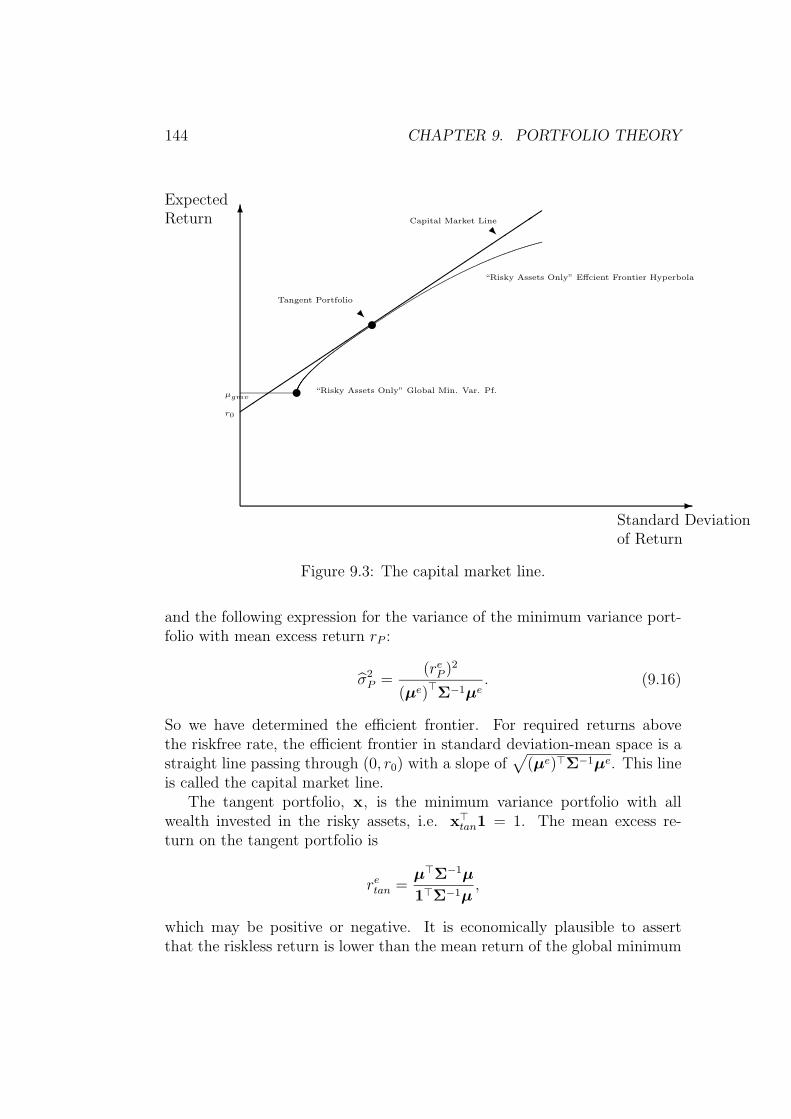
144 CHAPTER 9. PORTFOLIO THEORY
u “Risky Assets Only” Global Min. Var. Pf.
6
-
uRTangent Portfolio
r0
µgmv
Capital Market Line
R
“Risky Assets Only” Effcient Frontier Hyperbola
ExpectedReturn
Standard Deviationof Return
Figure 9.3: The capital market line.
and the following expression for the variance of the minimum variance port-folio with mean excess return rP :
σ2P =
(reP )2
(µe)>Σ−1µe. (9.16)
So we have determined the efficient frontier. For required returns abovethe riskfree rate, the efficient frontier in standard deviation-mean space is astraight line passing through (0, r0) with a slope of
√(µe)>Σ−1µe. This line
is called the capital market line.The tangent portfolio, x, is the minimum variance portfolio with all
wealth invested in the risky assets, i.e. x>tan1 = 1. The mean excess re-turn on the tangent portfolio is
retan =µ>Σ−1µ
1>Σ−1µ,
which may be positive or negative. It is economically plausible to assertthat the riskless return is lower than the mean return of the global minimum
9.2. THE CAPITAL ASSET PRICING MODEL (CAPM) 145
variance portfolio of the risky assets. In this case the situation is as illustratedin Figure 9.3, and that explains why we use the term “tangency”. Whenretan > 0, the tangent portfolio is on the capital market line. But the tangentportfolio must also be on the “risky assets only” efficient frontier. So thestraight line (the CML) and the hyperbola intersect at a point correspondingto the tangency portfolio. But clearly the CML must be above the efficientfrontier hyperbola (we are minimizing variance with an extra asset). So theCML is a tangent to the hyperbola.
For any portfolio, P we define the Sharpe-ratio as excess return relativeto standard deviation,
Sharpe-ratioP =µP − r0
σP.
In the case where retan > 0, we see note from Figure 9.3 that the tangencyportfolio is the “risky assets only”-portfolio with the highest Sharpe-ratiosince the slope of the CML is the Sharpe-ratio of tangency portfolio. (Gen-erally/”strictly algebraically” we should say that xtan has maximal squaredSharpe-ratio.)
Note that a portfolio with full investment in the riskfree asset is orthogo-nal to any other portfolio; this means that we can prove the following resultin exactly the manner as Proposition 32.
Proposition 33 Let xmv be a portfolio on the mean-variance frontier withrate of return rmv, expected rate of return µmv and variance σ2
mv. Let xP bean arbitrary portfolio, and use similar notation for rates of return on theseportfolios. Then the following holds:
µP − r0 = βP,mv(µmv − r0),
where
βP,mv =Cov(rP , rmv)
σ2mv
.
9.2 The Capital Asset Pricing Model (CAPM)
With the machinery of portfolio optimization in place, we are ready to for-mulate one of the key results of modern finance theory, the CAPM-relation.Despite the clearly unrealistic assumptions on which the result is built it stillprovides invaluable intuition on what factors determine the price of assets inequilibrium. Note that until now, we have mainly been concerned with pric-ing (derivative) securities when taking prices of some basic securities as given.
146 CHAPTER 9. PORTFOLIO THEORY
Here we try to get more insight into what determines prices of securities tobegin with.
We consider an economy with n risky assets and one riskless asset. Here,we let ri denote the rate of return on the i’th risky asset and we let r0 denotethe riskless rate of return. We assume that r0 is strictly smaller than thereturn of the global minimum variance portfolio.
Just as in the case of only risky assets one can show that with a risklessasset the expected return on any asset or portfolio can be expressed as afunction of its beta with respect to an efficient portfolio. In particular, sincethe tangency portfolio is efficient we have
Eri − r0 = βi,tan(Ertan − r0) (9.17)
where
βi,tan =Cov(ri, rtan)
σ2tan
(9.18)
The critical component in deriving the CAPM is the identification of thetangency portfolio as the market portfolio. The market portfolio is definedas follows: Assume that the initial supply of risky asset j at time 0 has avalue of P j
0 . (So P j0 is the number of shares outstanding times the price per
share.) The market portfolio of risky assets then has portfolio weights givenas
wmj =P 0j∑n
i=1 P0i
(9.19)
Note that it is quite reasonable to think of a portfolio with these weights asreflecting “the average of the stock market”.
Now if all (say K) agents are mean-variance optimizers (given wealths ofWi(0) to invest), we know that since there is a riskless asset they will hold acombination of the tangency portfolio and the riskless asset since two fundseparation applies. Hence all agents must hold the same mix of risky assetsas that of the tangency portfolio. This in turn means that in equilibriumwhere market clearing requires all the risky assets to be held, the marketportfolio (which is a convex combination of the individual agents’ portfolios)has the same mixture of assets as the tangency portfolio. Or in symbols: Letφi denote the fraction of his wealth that agent i has invested in the tangencyportfolio. By summing over all agents we get
Total value of asset j =K∑i=1
φiWi(0)xtan(j)
= xtan(j)× Total value of all risky assets,
9.2. THE CAPITAL ASSET PRICING MODEL (CAPM) 147
where we have used that market clearing condition that all risky assets mustbe held by the agents. (This is a very weak consequence of equilibrium; somewould just call it an accounting identity. The main economic assumption isthat agents are mean-variance optimizers so that two fund separation ap-plies.) Hence we may as well write the market portfolio in equation (9.17).This is the CAPM:
Eri − r0 = βi,m(Erm − r0) (9.20)
where βi,m is defined using the market portfolio instead of the tangencyportfolio. Note that the type of risk for which agents receive excess returnsare those that are correlated with the market. The intuition is as follows: Ifan asset pays off a lot when the economy is wealthy (i.e. when the return ofthe market is high) that asset contributes wealth in states where the marginalutility of receiving extra wealth is small. Hence agents are not willing to payvery much for such an asset at time 0. Therefore, the asset has a high return.The opposite situation is also natural at least if one ever considered buyinginsurance: An asset which moves opposite the market has a high pay off instates where marginal utility of receiving extra wealth is high. Agents arewilling to pay a lot for that at time 0 and therefore the asset has a low return.Indeed it is probably the case that agents are willing to accept a return onan insurance contract which is below zero. This gives the right intuition butthe analogy with insurance is actually not completely accurate in that therisk one is trying to avoid by buying an insurance contract is not linked tomarket wide fluctuations.
Note that one could still view the result as a sort of relative pricing resultin that we are pricing everything in relation to the given market portfolio.To make it more clear that there is an equilibrium type argument underlyingit all, let us see how characteristics of agents help in determining the riskpremium on the market portfolio. Consider the problem of agent i in the oneperiod model. We assume that returns are multivariate normal and that theutility function is twice differentiable and concave1:
maxw
E(ui(Wi1))
s.t.W i1 = W0(w>r + (1−w>1)r0)
When forming the Lagrangian of this problem, we see that the first ordercondition for optimality is that for each asset j and each agent i we have
E(u′i(W
i1)(rj − r0)
)= 0 (9.21)
1This derivation follows Huang and Litzenberger: Foundations for Financial Economics
148 CHAPTER 9. PORTFOLIO THEORY
Remembering that Cov(X, Y ) = EXY − EXEY we rewrite this as
E(u′i(W
i1))E(rj − r0) = −Cov(u′i(W
i1), rj)
A nice lemma known as Stein’s lemma says that for bivariate normal distri-bution (X, Y ) we have
Cov(g(X), Y ) = Eg′(X)Cov(X,Y )
and using this we have the following first order condition:
E(u′i(W
i1))E(rj − r0) = −Eu′′i (W i
1)Cov(W i1, rj)
i.e.−E (u′i(W
i1))E(rj − r0)
Eu′′i (Wi1)
= Cov(W i1, rj)
Now define the following measure of agent i’s absolute risk aversion:
θi :=−Eu′′i (W i
1)
Eu′i(Wi1)
.
Then summing across all agents we have that
E(rj − r0) =1∑Ki=1
1θi
Cov(W1, rj)
=1∑Ki=1
1θi
W0Cov(rm, rj)
where the total wealth at time 1 held in risky assets is W1 =∑K
i=1 Wi1, W0
is the total wealth in risky assets at time 0, and
rm =W1
W0
− 1
therefore is the return on the market portfolio. Note that this alternativerepresentation tells us more about the risk premium as a function of theaggregate risk aversion across agents in the economy. By linearity we alsoget that
Erm − r0 = WM0 V ar(rm)
1∑Ki=1
1θi
,
which gives a statement as to the actual magnitude expected excess returnon the market portfolio. A high θi corresponds to a high risk aversion andthis contributes to making the risk premium larger, as expected. Note that if

9.2. THE CAPITAL ASSET PRICING MODEL (CAPM) 149
one agent is very close to being risk neutral then the risk premium (holdingthat person’s initial wealth constant) becomes close to zero. Can you explainwhy that makes sense?
The derivation of the CAPM when using returns is not completely clearin the sense that finding an equilibrium return does not separate out whatis found exogenously and what is found endogenously. One should thinkof the equilibrium argument as determining the initial price of assets givenassumptions on the distribution of the price of the assets at the end of theperiod. A sketch of how the equilibrium argument would run is as follows:
1. Given the expected value and the covariance of end of period assetprices for all assets
2. Given a utility function for each investor which depends only on meanand variance of end-of-period wealth. Assume that utility decreases asa function of variance and increases as a function of mean. Assumealso sufficient differentiability
3. Let investor i have an initial fraction of the total endowment of riskyasset j.
4. Assume that there is riskless lending and borrowing at a fixed rate r.Hence the interest rate is exogenous.
5. Given initial prices of all assets, agent i chooses portfolio weights onrisky assets to maximize end of period utility. The difference in pricebetween the initial endowment of risky assets and the chosen portfolioof risky assets is borrowed n/placed in the money market at the risklessrate. (In equilibrium where all assets are being held this implies zeronet lending/borrowing.)
6. Compute the solution as a function of the initial prices.
7. Find a set of initial prices such that markets clear, i.e such that thesum of the agents positions in the risky assets sum up to the initialendowment of assets.
8. The prices will reflect characteristics of the agents’ utility functions,just as we saw above.
9. Now it is possible to derive the CAPM relation by computing expectedreturns etc. using the endogenously determined initial prices. This isa purely mathematical exercise translating the formula for prices intoformulas involving returns.
150 CHAPTER 9. PORTFOLIO THEORY
Hence CAPM is to be thought of as an equilibrium argument explaining assetprices.
There are of course many unrealistic assumptions underlying the CAPM.The distributional assumptions are clearly problematic. Even if basic secu-rities like stocks were well approximated by normal distributions there is nohope that options would be well approximated due to their truncated payoffs.An answer to this problem is to go to continuous time modelling where ’localnormality’ holds for very broad classes of distributions but that is outsidethe scope of this course. Note also that a conclusion of CAPM is that allagents hold the same mixture of risky assets which casual inspection showis not the case. A final problem, originally raised by Roll (1977)2, concernsthe observability of the market portfolio and the logical equivalence betweenthe statement that the market portfolio is efficient and the statement thatthe CAPM relation holds. To see that observability is a problem think forexample of human capital. Economic agents face many decisions over a lifetime related to human capital - for example whether it is worth taking a loanto complete an education, weighing off leisure against additional work whichmay increase human capital etc. Many empirical studies use all traded stocks(and perhaps bonds) on an exchange as a proxy for the market portfolio butclearly this is at best an approximation. And what if the test of the CAPMrelation is rejected using that portfolio? The relation At the intuitive level,the (9.17) tells us that this is equivalent to the inefficiency of the chosenportfolio. Hence one can always argue that the reason for rejection was notthat the model is wrong but that the market portfolio is not chosen correctly(i.e. is not on the portfolio frontier). Therefore, it becomes very hard totruly test the model. While we are not going to elaborate on the enormousliterature on testing the CAPM, note also that even at first glance it is noteasy to test what is essentially a one period model. To get estimates of thefundamental parameters (variances, covariances, expected returns) one willhave to assume that the model repeats itself over time, but when firms changethe composition of their balance sheets they also change their betas.
Hence one needs somehow to accommodate betas which change over timeand this inevitably requires some statistical compromises.
2R. Roll (1977): A critique of the asset pricing theory’s test; Part I, Journal of FinancialEconomics, 4:pp 129 - 76
9.3. RELEVANT, BUT NOT PARTICULARLY STRUCTURED, REMARKS ON CAPM151
9.3 Relevant, but not particularly structured,
remarks on CAPM
9.3.1 Systematic and non-systematic risk
This section follows Huang and Litzenberger’s Chapters 3 and 4. We havetwo versions of the capital asset pricing model. The most “popular” version,where we assumed the existence of a riskless asset whose return is r0, statesthat the expected return on any asset satisfies
Eri − r0 = βi,m(Erm − r0). (9.22)
This version we derived in the previous section. The other version is theso-called zero-beta CAPM, which replaces the return on the riskless asset bythe expected return on m′s zero-covariance portfolio:
Eri − Erzm = βi,m(Erm − Erzm).
This version is proved by assuming mean-variance optimizing agents, usingthat two-fund separation then applies, which means that the market portfoliois on the mean-variance locus (note that we cannot talk about a tangentportfolio in the model with no riskfree asset) and using Proposition 32. Notethat both relations state that excess returns (i.e. returns in addition to theriskless returns) are linear functions of βim.
From now on we will work with the case in which a riskless asset exists, butit is easy to translate to the zero-beta version also. Dropping the expectations(and writing “error terms” instead) we have also seen that if the marketportfolio m is efficient, the return on any portfolio (or asset) q satisfies
rq = (1− βq,m)rf + βq,mrm + εq,m
whereEεq,m = Eεq,mrm = 0.
HenceVar(rq) = β2
q,mVar (rm) + Var(εq,m).
This decomposes the variance of the return on the portfolio q into its system-atic risk β2
qmVar (rm) and its non-systematic or idiosyncratic risk Var(εq,m).The reason behind this terminology is the following: We know that there ex-ists a portfolio which has the same expected return as q but whose varianceis β2
qmVar (rm) - simply consider the portfolio which invests 1 − βqm in theriskless asset and βq,m, in the market portfolio. On the other hand, since this
152 CHAPTER 9. PORTFOLIO THEORY
portfolio is efficient, it is clear that we cannot obtain a lower variance if wewant an expected return of Erq. Hence this variance is a risk which is corre-lated with movements in the market portfolio and which is non-diversifiable,i.e. cannot be avoided if we want an expected return of Erq. On the otherhand as we have just seen the risk represented by the term VAR(εq,m) canbe avoided simply by choosing a different portfolio which does a better jobof diversification without changing expected return.
9.3.2 Problems in testing the CAPM
Like any model CAPM builds on simplifying assumptions. The model ispopular nonetheless because of its strong conclusions. And it is interestingto try and figure out whether the simplifying assumptions on the behavior ofindividuals (homogeneous expectations) and on the institutional setup (notaxation, transactions costs) of trading are too unrealistic to give the modelempirical relevance. What are some of the obvious problems in testing themodel?
First, the model is a one period model. To produce estimates of meanreturns and standard deviations, we need to observe years of price data. Canwe make sure that the distribution of returns over several years remain thesame3?
Second (and this a very important problem) what is the ’market portfo-lio’ ? Since investments decisions of firms and individuals in real life are notrestricted to stocks and bonds but include such things as real estate, edu-cation, insurance, paintings and stamp collections, we should include theseassets as well, but prices on these assets are hard to get and some are nottraded at all.
A person rejecting the CAPM could always be accused of not havingchosen the market portfolio properly. However, note that if ’proper choice’of the market portfolio means choosing an efficient portfolio then this ismathematically equivalent to having the CAPM hold.
This point is the important element in what is sometimes referred to asRoll’s critique of the CAPM. When discussing the CAPM it is important toremember which facts are mathematical properties of the portfolio frontierand which are behavioral assumptions. The key behavioral assumption ofthe CAPM is that the market portfolio is efficient. This assumption givesthe CAPM-relation mathematically. Hence it is impossible to separate theclaim ’the portfolio m is efficient’ from the claim that ’CAPM holds withm acting as market portfolio’.
3Mulitiperiod versions exist, but they also face problems with time varying parameters.
9.3. RELEVANT, BUT NOT PARTICULARLY STRUCTURED, REMARKS ON CAPM153
9.3.3 Testing the efficiency of a given portfolio
Since the question of whether CAPM holds is intimately linked with thequestion of the efficiency of a certain portfolio it is natural to ask whetherit is possible to devise a statistical test of the efficiency of a portfolio withrespect to a collection of assets. If we knew expected returns and variancesexactly, this would be a purely mathematical exercise. However, in practiceparameters need to be estimated and the question then takes a more statis-tical twist: Given the properties of estimators of means and variances, canwe reject at (say) a 5% level that a certain portfolio is efficient? Gibbons,Ross and Shanken (Econometrica 1989, 1121-1152) answer this question -and what follows here is a sketch of their test.
Given a portfolio m and N assets whose excess returns are recorded in Ttime periods. It is assumed that a sufficiently clear concept of riskless returncan be defined so that we can really determine excess returns for each period.NOTE: We will change our notation in this section slightly and assume thatrp, Erp and µp refer to excess returns, mean excess returns and estimatedmean excess returns of an asset or portfolio p. Hence using this notation theCAPM with a riskless asset will read
Erp = βp,mErm.
We want to test this relation or equivalently whetherm is an efficient portfolioin a market consisting of N assets. Consider the following statistical modelfor the excess returns of the assets given the excess return on the portfoliom :
rit = αi + γi rmt + εit
i = 1, . . . , N and t = 1, . . . ., T
where rit is the (random) excess return4 of asset i in the t′th period, rmtis the observed excess return on the portfolio in the t′th period, αi, γi areconstants and the εit’s are normally distributed with Cov(εit, εjt) = σij andCov(εit, εis) = 0 for t 6= s. Given these data a natural statistical representa-tion of the question of whether the portfolio m is efficient is the hypothesisthat α1 = · · · = αN = 0. This condition must hold for (9.22) to hold.
To test this is not difficult in principle (but there are some computationaltricks involved which we will not discuss here): First compute the MLE’sof the parameters. It turns out that in this model this is done merely bycomputing Ordinary Least Squares estimators for α, γ and the covariance
4Note this change to excess returns.
154 CHAPTER 9. PORTFOLIO THEORY
matrix for each period Σ. A so-called Wald test of the hypothesis α = 0 canthen be performed by considering the test statistic
W0 = αV ar(α)α−1
which you will learn more about in a course on econometrics. Here we simplynote that the test statistic measures a distance of the estimated value ofα from the origin. Normally, this type of statistics leads to an asymptoticchi squared test, but in this special model the distribution can be foundexplicitly and even more interesting from a finance perspective, it is shownin GRS that W0 has the following form
W0 =(T −N − 1)
N
(µ2q
σ2q− µ2
m
σ2m
)(
1 + µ2m
σ2m
)where the symbols require a little explanation: In the minimum varianceproblem with a riskless asset we found that the excess return of any portfoliosatisfies
Erp = βpmErm.
We refer to the quantityErpσ(rp)
as the Sharpe ratio for portfolio p. The Sharpe ratio in words compares excessreturn to standard deviation. Note that using the CAPM relation we canwrite
Erpσ(rp)
=σ(rm)ρmpσ2(rm)
(Erm)
where ρmp is the correlation coefficient between the return of portfolios p andm. From this expression we see that the portfolio which maximizes the Sharperatio is (proportional) to m.Only portfolios with this Sharpe ratio are effi-cient. Now the test statistic W0 compares two quantities: On one side, themaximal Sharpe ratio that can be obtained when using for parameters inthe minimum variance problem the estimated covariance matrix and the es-timated mean returns for the economy consisting of the N assets and theportfolio m. On the other side, the Sharpe ratio for the particular portfoliom (based on its estimated mean return and standard deviation).
Large values of W0 will reject the hypothesis of efficiency and this corre-sponds to a case where the portfolio m has a very poor expected return perunit of standard deviation compared to what is obtained by using all assets.
Chapter 10
The APT model
10.1 Introduction
Although the APT stands for ’Arbitrage Pricing Theory’ the model presentedhere is somewhat different from the arbitrage models presented earlier. Theframework is in one sense closer to CAPM in that we consider a one-periodmodel with risky assets whose distributions may be continuous. On theother hand, there is also a clear analogue with arbitrage pricing. We willpresent the basic idea of the model in two steps which will illustrate how therestriction on mean return arises.
10.2 Exact APT with no noise
Consider the following model for the returns r1, . . . , rN of N risky assets:
r = µ+Bf
where r = (r1, . . . , rN)> is a vector of random returns, µ = (µ1, . . . , µN)> ,and B is an N × K−matrix whose entries are real numbers, and f =(f1, . . . , fK) is a vector of random variables (factors) which satisfies
Efi = 0, i = 1, . . . , K,
Cov(f) = Φ, Φ positive definite.
Note that this means that Eri = µi , i = 1, . . . , N. We will assume thatN > K, and you should think of the number of assets N as being muchlarger than the number of factors K. The model then seeks to capture theidea that returns on assets are correlated through a common dependence ona (small) number of factors. The goal is to use the assumption of such a
155
156 CHAPTER 10. THE APT MODEL
common dependence to say something about the vector of mean returns µ.Assume that there is also a riskless asset with return r0. When we talk abouta portfolio, w, we mean a vector in RN where the ith coordinate measuresthe relative share of total wealth invested in the ith risky asset, and the restin the riskfree asset. (So the term ’investment strategy given by w’ wouldprobably be better). Hence the coordinates need not sum to 1, and theexpected rate of return on w is
E((1− w>1)r0 + w>r) = r0 + E(w>(r − r01))
= r0 + w>(µ− r01), (10.1)
where as usual 1 = (1, . . . , 1) ∈ RN .Since N > K it is possible to find a portfolio w ∈ RN of risky assets
which is orthogonal to the column space of B. This we will write as w ∈ (B)⊥.Now the mean return is r0 +w>(µ−1r0) and by using the “covariance matrixalgebra rules” in the first part of Chapter 9 we see that the variance of thereturn on this portfolio is given as
V (w>r) = Cov(w>Bf,w>Bf)
= w>BΦB>w = 0.
A reasonable no arbitrage condition to impose is that a portfolio consistingonly of risky assets which has zero variance should earn the same return asthe riskless asset. Hence the following implication should hold in an arbitragefree market:
w>1 = 1, w ∈ (B)⊥ : w>µ = r0 ⇐⇒ w>(µ− r01) = 0.
By scaling we see that
w>1 6= 0, w ∈ (B)⊥ : w>(µ− r01) = 0.
By using the same “arbitrage reasoning” on (10.1) we get that
w>1 = 0, w ∈ (B)⊥ : w>µ = 0⇐⇒ w>(µ− r01) = 0.
From these two statements we see that any vector which is orthogonal to thecolumns of B is also orthogonal to the vector (µ − r01), and this implies1
1If you prefer a mathematical statement, we are merely using the fact that
(B)⊥ ⊂ (µ− r01)⊥ =⇒ (µ− r01) ⊂ (B).
10.3. INTRODUCING NOISE 157
that µ − r01 is in the column span of B. In other words, there exists λ =(λ1, . . . , λK) such that
µ− r01 =Bλ. (10.2)
The vector λ = (λ1, . . . , λK) is called the vector of factor risk premia andwhat the relation tells us is that the excess return is obtained by multiplyingthe factor loadings with the factor risk premia. This type of conclusion is ofcourse very similar to the conclusion of CAPM, in which there is ’one factor’(return on the market portfolio), βim plays the role of the factor loading andErm − r0 is the factor risk premium.
10.3 Introducing noise
We continue the intuition building by considering a modification of the modelabove. Some of the reasoning here is heuristic - it will be made completelyrigorous below.
Assume thatr = µ+Bf + ε
where r, µ,B and f are as above and ε = (ε1, . . . , εN) is a vector of randomvariables (noise terms or idiosyncratic risks) satisfying
Eεi = 0, i = 1, . . . , N,
Cov(εi, fj) = 0, i = 1, . . . , N, j = 1, . . . , K,
Cov(ε) = σ2IN , IN is the N ×N identity matrix.
Clearly, this is a more realistic model since the returns are not completelydecided by the common factors but ’company specific’ deviations capturedby the noise terms affect the returns also. However if the variance in thenoise term is not too large then we can almost eliminate the variance arisingfrom the noise term through diversification.
Since N > K it is possible to find portfolios of risky assets v1, . . . , vN−Kwhich are orthogonal and lie in (B)⊥. Let a be the maximal absolute valueof the individual portfolio weights. Now consider the portfolio
v =1
N −K(v1 + · · ·+ vN−K).
The variance of the return of this portfolio is
V(v>r) = V(v>Bf + v>ε)
= 0 +1
(N −K)2 V((v1 + · · ·+ vN−K)>ε)
158 CHAPTER 10. THE APT MODEL
≤ 1
(N −K)2(N −K)a2σ2
=a2σ2
N −K,
where the inequality follows from the orthogonality of the vi’s (and the defi-nition of a).
If we think of N as very large, this variance is very close to 0, and -entering into heuristic mode - therefore the expected return of this portfolioought to be close to that of the riskless asset:
Ev>r = v>µ ≈ r0. (10.3)
By a slight modification of this argument it is possible to construct portfolioswith good diversification which span (B)⊥ and for each portfolio we derivea relation of the type (10.3). This then would lead us to expect that thereexists factor risk premia such that
µ− r01 ≈Bλ.
The precise theorem will be given below.
10.4 Factor structure in a model with infinitely
many assets
In this section we present a rigorous version of the APT.Given is a riskless asset with return r0 and an infinite number of risky
assets with random returns (r1, r2, . . .). We will use the following notationrepeatedly: If x = (x1, x2, . . .) is an infinite sequence of scalars or randomvariables, then xN is the column vector consisting of the first N elements ofthis sequence. Hence rN = (r1, . . . , rN)>.
Definition 41 The returns (r1, r2, . . .) are said to have an approximate fac-tor structure with factors (f1, . . . , fK) if for all N
rN = µN +BNf + εN
where BN is the N first rows of a matrix B with infinitely many rows andK columns, where BN has rank K for N large,
Eεi = 0, i = 1, 2, . . . ,
Cov(εi, fj) = 0, i = 1, 2, . . . , j = 1, . . . , K,
Cov(f) = IK (the K ×K identity matrix)
Cov(εN) = ΩN (ΩN is positive definite)
10.4. FACTOR STRUCTURE IN A MODEL WITH INFINITELY MANY ASSETS159
and where the eigenvalues of ΩN are bounded uniformly in N by a constantλ.
In other words, the same K factors are governing the returns on an infinitecollection of securities except for noise terms captured by ε which however areuniformly of small variance. The simplest case would be where the elementsof ε are independent2 and have variance less than or equal to σ2 in whichcase λ = σ2. Although our definition is slightly more general you can thinkof each element of ε as affecting only a finite number of returns and factorsas affecting infinitely many of the returns.
The assumption that the covariance matrix of the factors is the identitymay seem very restrictive. Note however, that if we have a structure of theform
r = µ+Bf + ε
which satisfies all the requirements of the definition of an approximate factorstructure with the only exception being that
Cov(f) = Φ (Φ is a positive definite, K ×K-matrix)
then using the representation Φ = CC> for some invertible K ×K matrixwe may choose g such that Cg = f. Then we have
r = µ+BCg + ε
and then this will be an approximate factor structure with g as factors andBC as factor loadings. To verify this note that
Cov(g) = C−1CC>(C−1)> = IK .
Hence in one sense nothing is lost by assuming the particular structureof f. We may represent the same distribution of returns in this way as ifwe allow a general positive definite matrix to be the covariance matrix ofthe factors. However, from a statistical viewpoint the fact that differentchoices of parameters may produce the same distributions is a cause foralarm. This means that we must be careful in saying which parameterscan be identified when estimating the model: Certainly, no observations candistinguish between parameters which produce the same distribution for thereturns. We will not go further into these problems and to discussions ofwhat restrictions can be imposed on parameters to ensure identification. Wenow need to introduce a modified notion of arbitrage:
2In this case the returns are said to have a strict factor structure.
160 CHAPTER 10. THE APT MODEL
Definition 42 An asymptotic arbitrage opportunity is a sequence of portfo-lios (wN),where wN ∈ RN , in the risky assets which satisfies
limN→∞
E(wN · rN) = ∞
and
limN→∞
V(wN · rN) = 0.
The requirement that expected return goes to infinity (and not just someconstant greater than the riskless return) may seem too strong, but in themodels we consider this will not make any difference.
The theorem we want to show, which was first stated by Ross and laterproved in the way presented here by Huberman, is the following:
Theorem 34 Given a riskless asset with return r0 > −1 and an infinitenumber of risky assets with random returns (r1, r2, ...).Assume that the re-turns have an approximate factor structure. If there is no asymptotic arbi-trage then there exists a vector of factor risk premia (λ1, . . . , λK) such thatwe have
∞∑i=1
(µi − r0 − λ1bi1 − · · · − λKbiK)2 <∞. (10.4)
This requires a few remarks: The content of the theorem is that theexpected excess returns of the risky assets are in a sense close to satisfyingthe exact APT-relation (10.2): The sum of the squared deviations from theexact relationship is finite. Note that (unfortunately) this does not tell usmuch about the deviation of a particular asset. Indeed the mean return ofan asset may show significant deviation from (10.2). This fact is crucial inunderstanding the discussion of whether the APT is a testable model.
The proof must somehow use the same arbitrage argument as in the casewith exact APT above by getting rid of the noise terms through diversifica-tion. Although this sounds easy, we discover once again that ’the devil is inthe details’. To do the proof we will need the following two technical lemmas:
Lemma 35 Let Ω be a symmetric positive definite N ×N matrix and let λbe its largest eigenvalue. Then
w>Ωw ≤ λ ‖w‖2 .
10.4. FACTOR STRUCTURE IN A MODEL WITH INFINITELY MANY ASSETS161
Proof Let (v1, . . . , vN) be an orthonormal set of eigenvectors of Ω and(λ1, . . . , λN) the corresponding eigenvalues. There exist α1, . . . , αN such thatw =
∑N1 αivi and hence
w>Ωw =N∑1
α2iλiv
>i vi
=N∑1
α2iλi
≤ λN∑1
α2i = λ ‖w‖2 .
Lemma 36 Let X be a compact set. Let (Ki)i∈I be a family of closed sub-sets of X which satisfy the finite intersection property⋂
i∈I0
Ki 6= ∅ for all finite subsets I0 ⊂ I.
Then the intersection of all sets is in fact non-empty. i.e.⋂i∈I
Ki 6= ∅.
Proof If⋂i∈I Ki = ∅, then
⋃i∈I K
ci is an open covering of X. Since X
is compact the open cover contains a finite subcover⋃i∈I0 K
ci , but then we
apparently have a finite set I0 for which⋂i∈I0 Ki = ∅, and this violates
the assumption of the theorem.
The proof is in two stages. First we prove the following:
Proposition 37 Given a riskless asset with return r0 > −1 and an in-finite number of risky assets with random returns (r1, r2, ...).Assume thatthe returns have an approximate factor structure. If there is no asymptoticarbitrage then there exists a sequence of factor risk premia vectors (λN),λN ∈ RK , and a constant A such that for all N
∞∑i=1
(µi − r0 − λN1 bi1 − · · · − λNKbiK)2 ≤ A. (10.5)
162 CHAPTER 10. THE APT MODEL
Proof Let us WLOG assume BNhas rank K for all N . Consider for each Nthe regression of the expected excess returns on the columns of BN , i.e. theλN ∈ RK that solves
minλ
(µN − r01−BNλN)>(µN − r01−BNλN) = min ||cN ||2
where the residuals are defined by
cN = µN − r01N −BNγN
By (matrix)-differentiating we get the first order conditions
(BN)>cN = 0
But the K ×K matrix (BN)>BN is invertible (by our rank K assumption),so the unique solution is
λN = ((BN)>BN)−1(BN)>(µN − r01).
We also note from the first order condition that the residuals cN are orthog-onal to the columns of BN . To reach a contradiction, assume that there isno sequence of factor risk premia for which (10.5) holds. Then we must have||cN || → ∞ (since ||cN ||2 is the left hand side of (10.5) with summation toN). Now consider the sequence of portfolios given by
wN =∥∥cN∥∥− 3
2 cN .
The expected excess return is given by
E(wN · (rN − r01N)) = E(wN · (µN − r01
N +BNf + εN))
= E(wN · (BNγN + cN +BNf + εN))
=∥∥cN∥∥− 3
2 cN · cN
=∥∥cN∥∥ 1
2 →∞ as N →∞.
where in the third equality we used the fact that cN is orthogonal to thecolumns of B and that both factors and noise terms have expectation 0. Thevariance of the return on the sequence of portfolios is given by
V(wN · (rN − r01N)) = V(wN · (µN − r01
N +BNf + εN))
= V(wN · εN)
=∥∥cN∥∥−3
(cN)>ΩNcN
≤∥∥cN∥∥−3
λ∥∥cN∥∥2 → 0 as N →∞
10.4. FACTOR STRUCTURE IN A MODEL WITH INFINITELY MANY ASSETS163
where we have used Lemma 35 and the same orthogonality relations as inthe expected return calculations. Clearly, we have constructed an asymptoticarbitrage opportunity and we conclude that there exists a constant A and asequence of factor risk premia such that
∞∑i=1
(µi − r0 − λN1 bi1 − · · · − λNKbiK)2 ≤ A.
Now we are ready to finish.Proof of Theorem 34 Let A be as in the proposition above. Consider thesequence of sets (HN) where
HN =
λ ∈ RK :
N∑i=1
(µi − r0 − λ1bi1 − · · · − λKbiK)2 ≤ A
.
By the preceding proposition, each HN is non-empty and clearly HN+1 ⊂HN . Define the functions fN : RK 7→ R by
fN(λ) = (µ−r01−Bλ)>(µ−r01−Bλ) = ||µ−r01||2+(µ−r01)>Bλ+λ>B>Bλ,
where some of the N -superscripts have been dropped for the ease of notation.Then fN is a convex function (because B>B is always positive semidefinite),and we see that
HN =λ ∈ RK : f(λ) ≤ A
is a closed convex set. Now pick an N so large that B has rank K. Toshow that HN is then compact, it suffices (by convexity) to show that forall nonzero λ ∈ HN there exists a scaling factor (a real number) a such thataλ 6∈ HN . But since B has full rank, there is no nonzero vector (in RK) thatis orthogonal to all of B’s (N) rows. Hence for an arbitrary nonzero λ ∈ HN
we have that ||Bλ|| 6= 0 and
fN(aλ) = ||µ− r01||2 + a(µ− r01)>Bλ+ a2||Bλ||2,
so by choosing a large enough a we go outside HN , so HN is not compact.Then we may use Lemma 36 to conclude that
∞⋂N=1
HN 6= ∅.
Any element λ = (λ1, . . . , λK)> of this non-empty intersection will satisfy10.4.

164 CHAPTER 10. THE APT MODEL
Chapter 11
On financial decisions of thefirm
11.1 Introduction
One may think of decisions of firms as divided into two categories: realdecisions and financial decisions. The real decisions focus on which projectsthe firms should undertake, the financial decisions deal with how the firmshould raise money to undertake the desired projects. The area of corporatefinance tries to explain the financial decisions of firms.
This chapter gives a very short introduction to the most basic issues in thisarea. The goal is to understand a couple of famous irrelevance propositionsset forth by Modigliani and Miller stating conditions under which the firmsfinancing decisions are in fact of no consequence. The conditions are infact very restrictive but very useful since any discussion on optimality andrationality of financing decisions must start by relaxing one or several of theseconditions.
We will consider only two types of securities: bonds and stocks. In realitythere are many other types of securities (convertible bonds, callable bonds,warrants,...) and an important area of research (security design) seeks toexplain why the different types of financing even exist. But we will haveenough to do just learning the basic terminology and the reader will certainlysee how to include more types of securities into the analysis.
Finally, it should be noted that a completely rigorous way of analyzingthe firm’s financing decisions requires general equilibrium theory - especiallya setup with incomplete markets - but such a rigorous analysis will take farmore time than we have in this introductory course.
165
166 CHAPTER 11. ON FINANCIAL DECISIONS OF THE FIRM
11.2 ’Undoing’ the firm’s financial decisions
At the heart of the irrelevance propositions are the investors ability to ’undo’the firm’s financial decision: If a firm changes the payoff profile of its debtand equity, the investor can under restrictive assumptions change his portfolioand have an unchanged payoff of his investments. We illustrate all this in aone-period, finite state space model.
Given two dates 0 and 1 and a finite state space with S states. Assumethat markets are complete and arbitrage free. Let ps denote the price of anArrow-Debreu security for state s, i.e. a security which pays 1 if the stateat date 1 is s and 0 in all other states. Assume that an investment policyhas been chosen by the firm which costs I0 to initiate at time 0 and whichdelivers a state contingent payoff at time 1 given by the vector (i.e. randomvariable) x = (x1, . . . , xS).
The firm at date 0 may choose to finance its investment by issuing debtmaturing at date 1 with face value D, and by issuing shares of stocks (equity).Assuming no bankruptcy costs, the payoff at the final date to equity and debtis given by the random variables
E1 = max(x−D, 0)
B1 = min(x,D)
respectively. If we assume that there are N shares of stocks, the payoff toeach stock is given by S1 = 1
NE1. Note that the entire cash flow to the
firm is distributed between debt and equity holders. If we define the valueof the firm at time 0 as the value at time 0 of the cash flows generated attime 1 minus the investment I0, it is clear that the value of the firm attime 0 is independent of the level of D. This statement is often presented asModigliani-Miller theorem but as we have set it up here (and as it is oftenpresented) it is not really a proposition but an assumption: The value of thefirm is by assumption unaffected by D since by assumption the payoff onthe investment is unaffected by the choice of D. As we shall see below, thischanges for example when there are bankruptcy costs or taxes.
Consider two possible financing choices: One in which the firm choosesto be an all equity (unlevered) firm and have D = 0, and one in which thefirm chooses a level of D > 0 (a levered firm). We let superscript U denotequantities related to the unlevered firm and let superscript L refer to the caseof a levered firm. By assumption V L = V U since the assumption of leverageonly results in a different distribution of the ’pie’ consisting of the firm’scash flows, not a change in the pie’s size. Now consider an agent who in hisoptimal portfolio in equilibrium wants to hold a position of one stock in the
11.2. ’UNDOING’ THE FIRM’S FINANCIAL DECISIONS 167
unlevered firm. The payoff at date 1 of this security is given by
SU1 =1
NEU
1 =1
Nx.
If the firm decides to become a levered firm, the payoff of one stock in thefirm becomes
SL1 =1
Nmax(x−D, 0)
which is clearly different from the unlevered case. However note the following:Holding 1
Nshares in the levered firm and the fraction 1
Nof the firms debt,
produces a payoff equal to
1
Nmax(x−D, 0) +
1
Nmin(x,D) =
1
Nx.
From this we see that even if the firm changes from an unlevered to a leveredfirm, the investor can adapt to his preferred payoff by changing his portfolio(something he can always do in a complete market). Similarly, we note fromthe algebra above that it is possible to create a position in the levered firm’sstock by holding one share of unlevered stock and selling the fraction 1
N
of the firm’s debt. In other words, the investor is able to undo the firm’sfinancial decision. In general equilibrium models this implies, that if thereis an equilibrium in which the firm chooses no leverage, then there is alsoan equilibrium in which the firm chooses leverage and the investors chooseportfolios to offset the change in the firm’s financing decision. This meansthat the firm’s capital structure remains unexplained in this case and morestructure must be added to understand how a level of debt may be optimalin some sense.
It is important to note that something like complete markets is requiredand this is very restrictive. In real world terms, to imitate a levered stock inthe firm, the investor must be able to borrow at the same conditions as thefirm (highly unrealistic) and furthermore have the debt contract structuredin such a way, that it imitates the payoffs of the firm when it is in bankruptcy.
We now consider another financing decision at time 0, namely the divi-dend decision. We consider for simplicity a firm which is all equity financed.To give this a somewhat more realistic setup, imagine that we are in factconsidering the last period of a firm’s life and that it carries with it an ’en-dowment’ of cash W0 from previous periods, which you can also think of as’earnings’ from previous activity. Also, imagine that the firm has N sharesof stock outstanding initially. The value of the firm at time 0 is given by thevalue of the cash flows that the firm delivers to shareholders:
V0 = Div0 −∆E0 +∑s
psxs
168 CHAPTER 11. ON FINANCIAL DECISIONS OF THE FIRM
where Div0 is the amount of dividends paid at time 0 to the shareholders and∆E0 is the amount of new shares issued (repurchased if negative) at time 0.It must be the case that
W0 + ∆E0 = I0 +Div0
i.e. the initial wealth plus money raised by issuing new equity is used eitherfor investment or dividend payout. If the firm’s investment decision hasbeen fixed at I0 and W0 is given, then Div0 −∆E0 = W0 − I0 is fixed, andsubstituting this into the equation for firm value tells us that firm valueis independent of dividends when the investment decision is given. Thedividend payment can be financed with issuing stocks. This result is alsosometimes referred to as the Modigliani-Miller theorem.
But you might think that if the firm issues new stock to pay for a dividendpayout, it dilutes the value of the old stocks and possibly causes a loss tothe old shareholders. In the world with Arrow-Debreu prices this will nothappen:
Consider a decision to issue new stocks to finance a dividend payment ofDiv0.Assume for simplicity that I0 = W0. The number of stocks issued toraise Div0 amount is given by M where
Div0 =M
N +M
∑s
psxs.
The total number of stocks outstanding after this operation is M + N andthe value that the old stockholders are left with is the sum of the dividendand the diluted value of the stocks, i.e.
Div0 +N
N +M
∑s
psxs
=M
N +M
∑s
psxs +N
N +M
∑s
psxs
=∑s
psxs
which is precisely the value before the equity financed dividend payout. Thismeans that the agent who depends in his optimal portfolio choice on no div-idends can undo the firm’s decision to pay a dividend by taking the dividendand investing it in the firms equity. Similarly, if a dividend is desired at time0 but the firm does not provide one, the investor can achieve it by sellingthe appropriate fraction of his stock position. The key observation is that aslong as the value of the shareholders position is unchanged by the dividend
11.3. TAX SHIELD 169
policy, the investor can use complete financial markets to design the desiredcash flow.
A critical assumption for dividends to have no effect on the value of thefirm and on the shareholder’s wealth is that income from dividend payoutsand income from share repurchases are taxed equally - something which isnot true in many countries. If there is a lower tax on share repurchases itwould be optimal for investors to receive no dividends and have any differencebetween W0 and I0 paid out by a share repurchase by the firm. Historically,one has observed dividend payouts even when there is lower taxes on sharerepurchases. Modigliani-Miller then tells us that something must be going onin the real world which is not captured by our model. The most importantreal world feature which is not captured by our model is asymmetric infor-mation. Our model assumes that everybody agrees on what the cash flowsof the firm will be in each state in the future. In reality, there will almost al-ways be insiders (managers and perhaps shareholders) who know more aboutthe firm’s prospects than outsiders (potential buyers of stocks, debtholders)and both the dividend policy and the leverage may then be used to signalto the outside world what the prospects of the firm really are. Changing theoutsider’s perception of the firm may then change the value of the firm.
11.3 Tax shield
If we change the model a little bit and assume that there are corporatetaxes but that equity and debt financing are treated differently in the taxcode then the capital structure becomes important. Change the model byassuming that the cash flows at time 1 are taxed at a rate of τ c but thatinterest payments on debt can be deducted from taxable income. Let rDdenote the part of the debt repayment which is regarded as ’interest’. Theafter tax cash flow of an unlevered firm at time 1 is given by
V U1 = (1− τ c)x
whereas the after tax cash flow of the levered firm (assuming full deductionof interest in all states) is given by
V L1 = rD + (1− τ c)(x− rD).
The difference in the cash flows is therefore
V L1 − V U
1 = τ crD
170 CHAPTER 11. ON FINANCIAL DECISIONS OF THE FIRM
which means that the levered firm gets an increased value of
V L0 − V U
0 = τ crD∑s
ps.
As D increases, so does the value of this tax shield. Hence, in this setupfinancing the firm’s operations with debt only would be optimal. But ofcourse, it would be hard to convince tax authorities that a 100% debt financ-ing was not actually a 100% equity financing! On the other hand, it shouldat least be the case that a significant fraction of debt was used for financingwhen there is a tax shield.
11.4 Bankruptcy costs
However, using a very high level of debt also increases the probability ofbankruptcy. And it would add realism to our model if we assumed that whenbankruptcy occurs, lawyers and accountants receive a significant fraction ofthe value left in the firm. This means that the total remaining value ofthe firm is no longer distributed to debtholders, and the debtholders willtherefore have an interest in making sure that the level of debt issued by afirm is kept low enough to reduce the risk of bankruptcy to an acceptablelevel.
The trade-off between gains from leverage resulting from a tax shieldand losses due to the increased likelihood of bankruptcy gives a first shot atdefining an optimal capital structure. This is done in one of the exercises.
11.5 Financing positive NPV projects
We have seen earlier that in a world of certainty, one should only start aproject if it has positive NPV. When uncertainty enters into our modelsthe NPV criterion is still interesting but we need of course to define anappropriate concept of NPV. Both the arbitrage-free pricing models and theCAPM models gave us ways of defining present values of uncertain incomestreams.
We consider a one-period, finite state space model in which there is acomplete, arbitrage-free market. Denote state prices (Arrow-Debreu prices)by p = (p1, . . . , pS). Assume that a firm initially (because of previous activity,say) has a net cash flow at time 1 given by the vector x = (x1 , . . . , xS).Thefirm is financed partly by equity and partly by debt, and firm value, equity
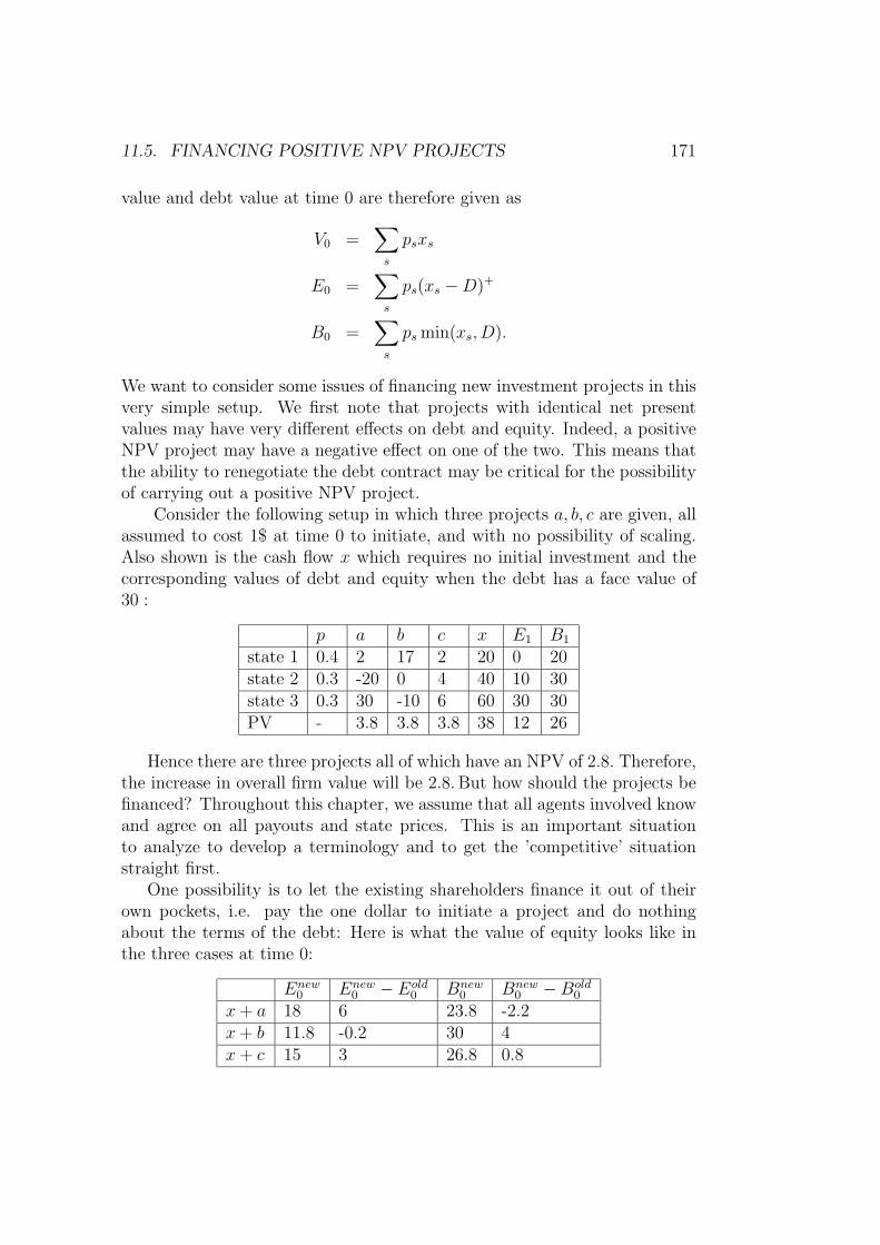
11.5. FINANCING POSITIVE NPV PROJECTS 171
value and debt value at time 0 are therefore given as
V0 =∑s
psxs
E0 =∑s
ps(xs −D)+
B0 =∑s
ps min(xs, D).
We want to consider some issues of financing new investment projects in thisvery simple setup. We first note that projects with identical net presentvalues may have very different effects on debt and equity. Indeed, a positiveNPV project may have a negative effect on one of the two. This means thatthe ability to renegotiate the debt contract may be critical for the possibilityof carrying out a positive NPV project.
Consider the following setup in which three projects a, b, c are given, allassumed to cost 1$ at time 0 to initiate, and with no possibility of scaling.Also shown is the cash flow x which requires no initial investment and thecorresponding values of debt and equity when the debt has a face value of30 :
p a b c x E1 B1
state 1 0.4 2 17 2 20 0 20state 2 0.3 -20 0 4 40 10 30state 3 0.3 30 -10 6 60 30 30PV - 3.8 3.8 3.8 38 12 26
Hence there are three projects all of which have an NPV of 2.8. Therefore,the increase in overall firm value will be 2.8.But how should the projects befinanced? Throughout this chapter, we assume that all agents involved knowand agree on all payouts and state prices. This is an important situationto analyze to develop a terminology and to get the ’competitive’ situationstraight first.
One possibility is to let the existing shareholders finance it out of theirown pockets, i.e. pay the one dollar to initiate a project and do nothingabout the terms of the debt: Here is what the value of equity looks like inthe three cases at time 0:
Enew0 Enew
0 − Eold0 Bnew
0 Bnew0 −Bold
0
x+ a 18 6 23.8 -2.2x+ b 11.8 -0.2 30 4x+ c 15 3 26.8 0.8
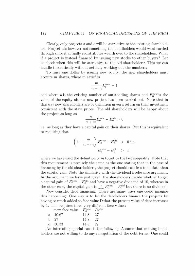
172 CHAPTER 11. ON FINANCIAL DECISIONS OF THE FIRM
Clearly, only projects a and c will be attractive to the existing sharehold-ers. Project a is however not something the bondholders would want carriedthrough since it actually redistributes wealth over to the shareholders. Whatif a project is instead financed by issuing new stocks to other buyers? Letus check when this will be attractive to the old shareholders: This we canhandle theoretically without actually working out the numbers:
To raise one dollar by issuing new equity, the new shareholders mustacquire m shares, where m satisfies
m
n+mEnew
0 = 1
and where n is the existing number of outstanding shares and Enew0 is the
value of the equity after a new project has been carried out. Note that inthis way new shareholders are by definition given a return on their investmentconsistent with the state prices. The old shareholders will be happy aboutthe project as long as
n
n+mEnew
0 − Eold0 > 0
i.e. as long as they have a capital gain on their shares. But this is equivalentto requiring that (
1− m
n+m
)Enew
0 − Eold0 > 0 i.e.
Enew0 − Eold
0 > 1
where we have used the definition of m to get to the last inequality. Note thatthis requirement is precisely the same as the one stating that in the case offinancing by the old shareholders, the project should cost less to initiate thanthe capital gain. Note the similarity with the dividend irrelevance argument.In the argument we have just given, the shareholders decide whether to geta capital gain of Enew
0 −Eold0 and have a negative dividend of 1$, whereas in
the other case, the capital gain is nn+m
Enew0 − Eold
0 but there is no dividend.Now consider debt financing. There are many ways one could imagine
this happening: One way is to let the debtholders finance the projects byhaving so much added to face value D that the present value of debt increasesby 1. This requires three very different face values:
new face value Enew0 Bnew
0
a 40.67 14.8 27b 27 14.8 27c 30,33 14.8 27
An interesting special case is the following: Assume that existing bond-holders are not willing to do any renegotiation of the debt terms. One could
11.5. FINANCING POSITIVE NPV PROJECTS 173
imagine for example, that the bondholders consisted of a large group of in-dividuals who cannot easily be assembled to negotiate a new deal. Now, ifproject bwere the only available project, then the shareholders would notenter into this project since the benefits of the project would go to the bond-holders exclusively. This is the so-called debt overhang problem where it isimpossible to finance a positive NPV project by issuing debt which is juniorto the existing debt. To be able to carry through with project b, the share-holders would have to talk the debtholders into reducing the face value ofthe debt.
In general, it is easy to see that if a project has positive NPV there existsa way of financing the project which will benefit both debt holders and equityholders (can you show this?).
A special case which one often sees mentioned in textbooks is the casewhere the new project is of the same ’risk class’ as the firm before enteringinto the project. This is true of project c. Such a project can always befinanced by keeping the same debt-equity ratio after the financing as before.This is also left to the reader to show.

174 CHAPTER 11. ON FINANCIAL DECISIONS OF THE FIRM
Chapter 12
Efficient Capital Markets
At the intuitive level, the efficient market hypothesis (EMH) states that it isimpossible to ”beat the market”: The return you earn by investing in finan-cial assets is proportional to the risk you assume. If certain assets had highreturns compared to their risks, investors - who are constantly searching forand analyzing information about companies, commodities, economic indica-tors, etc. - would rush to buy these assets, pushing up prices until returnswere ”proportional” to the risk. In this way information about future returnsof financial assets are quickly incorporated into prices which in other wordsfully and instantaneously reflect all available relevant information.
A first attempt to make this intuitive statement more rigorous is to elab-orate a little bit on the definition of ”relevant information” and to interpret’reflecting information’ as an inability to earn excessive returns. This leadsus to the famous degrees of efficiency:
1. Weak-form efficiency. No investor can earn excess returns developingtrading rules based on historical price or return information. In other words,the information in past prices or returns is not useful or relevant in achievingexcess returns.
2. Semistrong-form efficiency. No investor can earn excess returns fromtrading rules based on any publicly available information. Examples of pub-licly available information are annual reports of companies, investment advi-sory data such as ”Heard on the Street” in the Wall Street Journal, or tickertape information.
3. Strong-form efficiency. No investor can earn excess returns using anyinformation, whether publicly available or not.
Of course, we could define efficiency with respect to any information setIt: No trader can earn excess returns between time t and t + 1 given theinformation It.
Once we start thinking about this definition, however, we note that it is
175
176 CHAPTER 12. EFFICIENT CAPITAL MARKETS
still well short of being rigorous. What do we mean by ”risk” and by returnbeing ”proportional to risk”? And if indeed prices (in some sense) reflect allavailable information why are banks and other financial institutions payinganalysts to find information, and traders to ’look for arbitrage’ in the market?In this note we will analyze the problem of defining market efficiency asfollows:
First, we consider the problem of defining excess return. The only ’modelfree’ definition of this concept would be an arbitrage opportunity. Otherdefinitions are invariably linked to a particular model for security returns.If we are unable to find arbitrage opportunities can we then ever reject thehypothesis of ’market efficiency’?
Second, we consider some statistical properties of prices which are oftenthought of as being consequences of EMH. We try to give some rigorousdefinitions of these properties and (briefly) discuss if they are in any waynecessarily linked to market efficiency.
Third, we look at anomalies and a very interesting challenge to marketefficiency which attempts to show that stock prices are ’too volatile’ in thesense that they vary much more than accounted for by changes in economicfundamentals.
Finally we mention some attempts to make the definition of market effi-ciency completely rigorous in a general equilibrium context.
12.1 Excess returns
First, we try to make ”excess returns” a little more precise: As a first attemptwe could say that for any security P it must be the case that
E [Rt+1 | It] = 1 + rt (12.1)
where rt is the riskless rate of return at time t and
Rt+1 =Pt+1
Pt.
But having heard of CAPM and risk aversion we immediately object tothe use of rt: Assets with high risk (as measured e.g. through their β’s)should (and do!) earn more than the riskless rate. So we restate (12.1) as
E [Rt+1|It] = 1 + rPt (12.2)
where rPt is some return which is suitable for asset P. Note that we mayrewrite (12.2) as
1
1 + rPtE [Pt+1 | It] = Pt,
12.1. EXCESS RETURNS 177
which states that the properly discounted price is a martingale. If marketsare arbitrage free, such a discount factor will exist, so the requirement (12.2)is really nothing more than a statement of no arbitrage. In practice theproblem is to find a good model for rPt - indeed we spent a lot of time lookingat CAPM which tried to do just that. But if we have a model for rPt and wesee violations of (12.2), it would seem more natural to reject our model forrPt than to reject market efficiency. Assume for instance that we use CAPMto model rPt . The literature often refers to a rejection of (12.2) as a rejectionof ”a joint test of CAPM and market efficiency”. Given the very strongassumptions needed to derive CAPM, this is a somewhat strange statement(although it is of course logically OK). I would argue that unless there isa truly compelling and extremely realistic model (in terms of assumptionsdescribing markets accurately) for rPt , we should consider rejections of (12.2)as rejections of our choice of asset pricing model and not worry about themarket efficiency implications. Some proponents of efficient markets wouldsay that it is precisely the belief in efficient markets which causes us to rejectour model and look further for a rational explanation of stock price returns,and this is of course a valid point. But can we ever reach a situation in whichall conceivable models for rational behavior have been rejected and we haveno choice but to reject the EMH?
The closest to this situation would be a case where the model for rPt fol-lows from a no arbitrage condition. If, for example, we considered a portfolioof a written call, a put (both European with same exercise price and date)and a stock (the underlying security for both options), we know from put-call-parity that its return should equal the return on a zero-coupon bond.Violations of this relation which are large enough that traders may takeadvantage of it should clearly not persist in well functioning security mar-kets. In other words, no arbitrage is a necessary condition for markets tobe efficient. And only this provides a test of (12.2) which is not linked to aparticular choice of asset pricing model. Another way of stating this is thatwe can use (12.2) to test for violations of relative pricing relations which wederive from an assumption of no arbitrage. Violations would seem to indicatean inefficiency of markets.
But to use (12.2) as a definition of efficiency is complicated when we arelooking at ”absolute” quantities like stock prices. We will never be able toreject efficiency from this alone - critics will always (justly) be able to arguethat our choice of asset pricing model is wrong. A famous paper by DeBondtand Thaler1 [1986] illustrates the problem well. They did the following:
• Record the returns of a very large number of stocks over a period of1See Journal of Finance, July 1986, pp. 793-807.

178 CHAPTER 12. EFFICIENT CAPITAL MARKETS
Figure 12.1: The cumulative excess return (compared to the market) for the“winner” and “loser” portfolios.
(say) 36 months.
• At the end of the period, form one portfolio of ”winners” i.e. pick (say)the 35 best performing stocks of the 36 month period.
• Form another portfolio of ”losers” - i.e. pick (say) the 35 worst per-forming (but still alive!) stocks of the 36 month period.
• Compare the returns to that of the market.
The results are illustrated in Figure 12.1, which shows cumulative excessreturns compared to the market for the two portfolios. We see that the loserportfolio has a (quite large) positive return over the market, whereas “thewinners” are performing badly. Now we could be tempted to see this as aclear violation of ”weak-form efficiency” because, intuitively, we are beatingthe market using only information of past prices. But are we defining ”excessreturn” correctly then? We have seen in the exercises (in a discrete binomialversion) that the beta of an option on a stock may be related to the beta ofthe stock. The equivalent of this in a Black-Scholes model where we modelstocks as options on an underlying firm value gives us that
βS = N(d1)V
SβV .
12.2. MARTINGALES, RANDOM WALKS AND INDEPENDENT INCREMENTS179
A ”loser” stock will typically have experienced an increase in leverage. This inturn implies an increase in βS and therefore the increased return on a ”loser”follows directly from option pricing theory and CAPM. In other words, a morecareful selection of asset pricing model at least gave us a possible explanationfor the results of DeBondt and Thaler. Subsequent research (see for exampleChopra, Lakonishok and Ritter2 [1992]) seems to indicate that correcting forleverage effects does not destroy the result. But the controversy is far fromover and the key issue is whether more advanced asset pricing models can beshown to explain the larger returns on losing stocks. Note, however, that thecontroversy illustrates the sense in which (12.2) is a ”hard-to-test” definitionof efficiency. We will have to reject it for all conceivable (and reasonable)asset pricing models before an inefficiency is established. This seems to be atough task, especially considering results of Summers3 [1986] which indicatethat many test traditionally employed do not have very large power (i.e.ability to reject a false hypothesis).
12.2 Martingales, random walks and indepen-
dent increments
As a motivation for this section consider the footnote in Brealey and Myers:
”When economists speak of stock prices as following a random walk,they are being a little imprecise. A statistician reserves the term randomwalk to describe a series that has a constant expected change each periodand a constant degree of variability. But market efficiency does not implythat expected risks and expected returns cannot shift over time.”
Clearly, we need to be more precise even about the statistician’s definitionif we are to discuss the notions precisely. The purpose of this section is to giveprecise content to such concepts as random walk, independent increments andmartingales.
Definition 43 The stochastic process X = (X1, X2, . . .) is a random walkif it has the form
Xt =t∑i=1
εi
where ε1, ε2, . . . is a sequence of independent, identically distributed randomvariables.
2Journal of Financial Economics, 1992, pp. 235-2683Journal of Finance, July 1986, pp.591-601
180 CHAPTER 12. EFFICIENT CAPITAL MARKETS
We will normally assume that εi has finite variance (and hence finiteexpectation as well). If Eεi = 0 we say that the random walk is symmetric.
A weaker concept is that of a process with independent increments:
Definition 44 The stochastic process X = (X1, X2, . . .) is a process withindependent increments if for all t, ∆Xt ≡ Xt − Xt−1 is independent of(X1, X2, . . . , Xt−1).
Note that a random walk is a process with independent increments, but aprocess with independent increments may have the distribution of the incre-ment change with time. Weaker yet is the notion of orthogonal incrementswhere we only require increments to be uncorrelated:
Definition 45 The stochastic process X = (X1, X2, . . .) is a process withorthogonal increments if for all t , EX2
t <∞ and for all t, u
Cov(∆Xt,∆Xu) = 0.
Finally a somewhat different (but as we have seen equally important)concept
Definition 46 The stochastic process X = (X1, X2, . . .) is a martingale withrespect to the filtration (Ft) if for all t , E |Xt| <∞ and
E(Xt |Ft−1 ) = Xt−1.
If no filtration is specified it is understood that Ft−1 = σ(X1, X2, . . . , Xt−1).
A symmetric random walk is a martingale and so is a process with meanzero independent increments. A martingale with finite second moments hasorthogonal increments, but it need not have independent increments: Thinkfor example of the following ARCH process:
Xt = εtσt
where ε1, ε2, . . . is a sequence of i.i.d. N(0, 1) random variables and
σ2t = α0 + α1x
2t−1 α0, α1 > 0
where xt−1 is the observed value of Xt−1. The abbreviation ARCH stands forAutoregressive Conditional Heteroskedasticity which means (briefly stated)that the conditional variance of Xt given the process up to time t−1 dependson the process up to time t− 1.
12.3. ANOMALIES 181
It is clear from observation of market data, that stock prices have a driftand they are therefore not martingales. However it could be that by anappropriate choice of discount factor, as in (12.2), we get the martingaleproperty. In fact, we know that this will be possible in an arbitrage freemarket (and for all types of financial securities), but then we are back to thesituation discussed above in which the specification of the pricing relationbecomes essential.
The independent increment property is often heard as a necessary con-dition for efficient markets, but research over the last decade has pointed toARCH effects in stock prices, exchange rates and other financial securities.4
Another serious problem with all the properties listed above is that itis perfectly possible to construct sensible general equilibrium models (whichin particular are arbitrage free) in which prices and returns are serially cor-related (for example because aggregate consumption is serially correlated).Therefore, it seems unnatural to claim that random walks, independent incre-ments and martingale properties of prices are in any way logical consequencesof a definition of efficient markets. The most compelling consequence of anefficiency assumption of no arbitrage is that there exists an equivalent mea-sure under which securities are martingales but this does not in general saymuch about how processes behave in the real world. Indeed, even in thecase of futures contracts which would be very natural candidates to beingmartingales, we have seen that in models where agents are risk-averse, theequivalent martingale measure will in general be different from the empiri-cally measure and hence the martingale property of futures prices is by nomeans a necessary condition for efficiency.
Also, note that bonds for example have predetermined ’final’ value andtherefore it is not at all clear that any of the above mentioned properties ofprice processes are even relevant for this class of securities.
12.3 Anomalies
Another way to challenge the EMH is to look for strange patterns in securityprices which seem impossible to explain with any pricing model. Some suchanomalies are week-end effects and year-end effects:
Evidence found in French (1980)5 seems to suggest that returns on Mon-days were significantly negative, compared to returns on other trading days.Although the effect is difficult to exploit due to transactions costs, it is stillunclear why the effect exists. Possible explanations have tried to look at
4For an collection of papers see Engle: ARCH.Oxford University Press, 1995.5Journal of Financial Economics, 1980, pp. 55-69.
182 CHAPTER 12. EFFICIENT CAPITAL MARKETS
whether there is a tendency for firms to release bad news on Friday after-noons after trading closes. But if this were the case traders should learn thisan adjust prices accordingly earlier. The week-end effect is hard to explain -after all it does seem to suggest that traders who are going to trade anywayshould try to sell on Fridays and buy on Mondays.
Another effect documented in several studies is the year-end effect whichshows that stocks have a tendency to fall in December and rise in January.An obvious reason for such behavior could be tax considerations but it is stillunclear if this explanation is sufficient or whether there is actually an effectwhich trading rules can take advantage of.
A famous anomaly is the closed-end mutual fund discount. A closed-endfund is a mutual fund which holds publicly traded assets, but which onlyissues a fixed number of shares and where shareholders can only sell theirshares in the market. Since the assets are so easy to determine, so shouldthe share price be. However, throughout a long period of time mutual fundsseemed to sell at a discount: The values of the funds’ assets seemed largerthan the market value of shares. Small discounts could be explained bytax-considerations and illiquidity of markets, but no theory could explain apattern (shown in Figure 12.2) like the one observed for the TricontinentalCorporation6 during 1960-1986.
It seems that finally in 1986 prices adjusted, but that prices should ”in-stantaneously” have reflected fundamental information seems implausible.
So a newer version of EMH stated in Malkiel [1990]7 could be that ”pricingirregularities may well exist and even persist for periods of time, but thefinancial laws of gravity will eventually take hold and true value will comeout.” Certainly a weakening of our original version of efficiency.
12.4 Excess volatility.
One of the most interesting challenges to EMH argues that there is too muchvolatility in stock markets - more than can be explained by any sensible assetpricing theory. If indeed markets reflect all relevant information it should bethe case that price movements and arrival of new information were somehowin harmony. Trading alone ought not to generate volatility. Several pieces ofevidence suggest that trading ındeed creates volatility:
1. October 19, 1987. The Dow Jones Industrial Average fell by more than22% - a much bigger drop than any previous one-day movement. Yet exten-sive surveys among investment managers seem to suggest that no important
6See Lee, Shleifer and Thaler, Journal of Finance 1991, pp.75-109.7A Random Walk Down Wall Street.
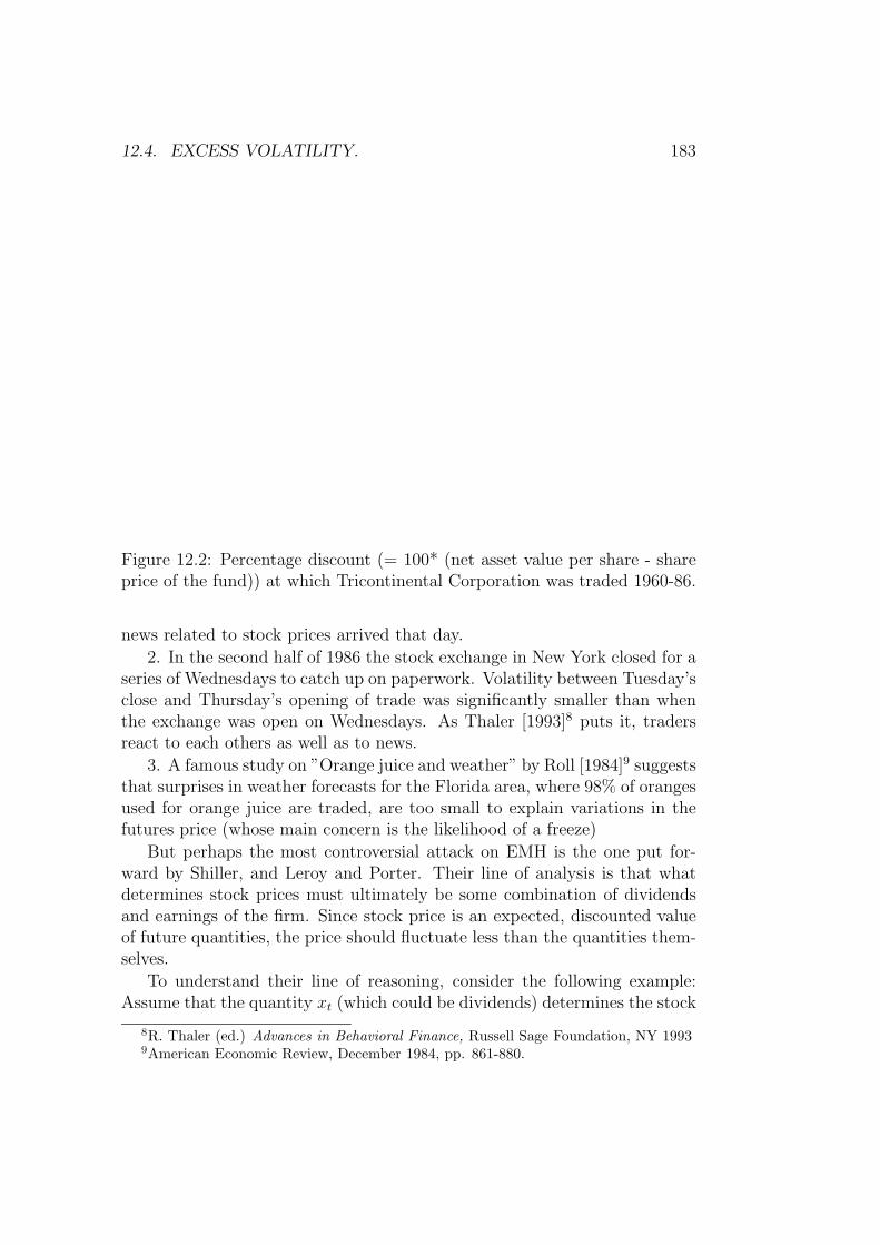
12.4. EXCESS VOLATILITY. 183
Figure 12.2: Percentage discount (= 100* (net asset value per share - shareprice of the fund)) at which Tricontinental Corporation was traded 1960-86.
news related to stock prices arrived that day.
2. In the second half of 1986 the stock exchange in New York closed for aseries of Wednesdays to catch up on paperwork. Volatility between Tuesday’sclose and Thursday’s opening of trade was significantly smaller than whenthe exchange was open on Wednesdays. As Thaler [1993]8 puts it, tradersreact to each others as well as to news.
3. A famous study on ”Orange juice and weather” by Roll [1984]9 suggeststhat surprises in weather forecasts for the Florida area, where 98% of orangesused for orange juice are traded, are too small to explain variations in thefutures price (whose main concern is the likelihood of a freeze)
But perhaps the most controversial attack on EMH is the one put for-ward by Shiller, and Leroy and Porter. Their line of analysis is that whatdetermines stock prices must ultimately be some combination of dividendsand earnings of the firm. Since stock price is an expected, discounted valueof future quantities, the price should fluctuate less than the quantities them-selves.
To understand their line of reasoning, consider the following example:Assume that the quantity xt (which could be dividends) determines the stock
8R. Thaler (ed.) Advances in Behavioral Finance, Russell Sage Foundation, NY 19939American Economic Review, December 1984, pp. 861-880.
184 CHAPTER 12. EFFICIENT CAPITAL MARKETS
price through a present value relation of the form:
Yt =∞∑j=0
βjXet (j),
where β is some discount factor, β ∈]0, 1[, and
Xet (j) = E[Xt+j|It],
where It can - for simplicity - be thought of as the information generated bythe process X up to time t. If we assume that Xt follows an autoregressiveprocess of order one, i.e.
Xt − c = φ(Xt−1 − c) + εt
where c > 0, |φ| < 1 and εt’s are independent normally distributed randomvariables, then we can calculate the coefficient of dispersion of Xt,
CD(Xt) =σ(Xt)
E(Xt)
and the similar quantity for Yt. We are interested in CD(Yt)CD(Xt)
. Using a factfrom time series analysis, which says that Xt be represented in the form
Xt − c =∞∑j=0
ϕj(εt−j)
we find
EXt = c V Xt =1
1− ϕ2
and
EYt =c
1− βV Yt =
V Xt
(1− βϕ)2
and henceCD(Yt)
CD(Xt)=
1− β1− βϕ
< 1
by our choice of parameters. In other words, the coefficient of dispersion foractual prices is less than that of Xt (dividends, earnings). What Shiller, andLeroy and Porter show is that this result holds for a large class of processesfor X and that the relationship is severely violated for observed data.
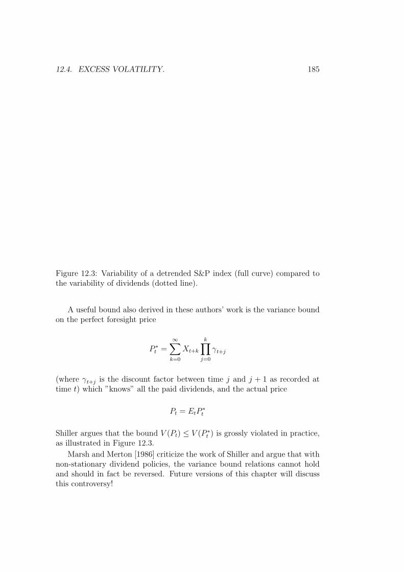
12.4. EXCESS VOLATILITY. 185
Figure 12.3: Variability of a detrended S&P index (full curve) compared tothe variability of dividends (dotted line).
A useful bound also derived in these authors’ work is the variance boundon the perfect foresight price
P ∗t =∞∑k=0
Xt+k
k∏j=0
γt+j
(where γt+j is the discount factor between time j and j + 1 as recorded attime t) which ”knows” all the paid dividends, and the actual price
Pt = EtP∗t
Shiller argues that the bound V (Pt) ≤ V (P ∗t ) is grossly violated in practice,as illustrated in Figure 12.3.
Marsh and Merton [1986] criticize the work of Shiller and argue that withnon-stationary dividend policies, the variance bound relations cannot holdand should in fact be reversed. Future versions of this chapter will discussthis controversy!
186 CHAPTER 12. EFFICIENT CAPITAL MARKETS
12.5 Informationally efficient markets are im-
possible
The title of this section is the title of a paper by Grossman and Stiglitz10
(1980) Their first paragraph in that work sums up an essential problem withthe assumption of informational efficiency:
”If competitive equilibrium is defined as a situation in which prices aresuch that all arbitrage profits are eliminated, is it possible that a compet-itive economy can always be in equilibrium? Clearly not, for then thosewho arbitrage make no (private) return from their (privately) costly activity.Hence the assumption that all markets, including that for information, arealways in equilibrium and always perfectly arbitraged are inconsistent whenarbitrage is costly.” Grossman and Stiglitz go on to build a model in whichgathering (costly) information is part of an equilibrium among informed anduninformed traders.Without going into details of their model, we note herethat in equilibrium, prices reflect some but not all of the information. Thereis a fraction of traders who are informed and spend money to gather infor-mation, and a fraction of traders who are uninformed but try to learn asmuch as possible by observing prices (which they know reflect partly theknowledge that the informed traders have). If some of the informed tradersgive up information gathering, prices will reflect less information and therewill be an incentive for non-informed traders to become informed becausethe costs of information gathering will more than compensated for by gainsfrom trade. If some uninformed traders in the equilibrium situation decideto become informed prices will reflect more information and there will in factbe an incentive for some of the informed to give up information gatheringand ’free-ride’ on the information gathered by others which is reflected inprices. Clearly, a situation in which all information is reflected in prices isimpossible.
This paper has a number of interesting results that we will not go intohere. Suffice it to say that it contains one of the most interesting attempts togive a formal definition of efficiency which does not have the inherent logicalproblems of the original definitions.
There are numerous other more rigorous attempts to define efficiency. Atypical line of approach is to model a situation with asymmetric informationand ask whether the equilibrium price (and possibly the portfolio holdingsof individuals) would be altered if all of the information held by traderswas given to all traders simultaneously. If prices and allocations would notchange in this situation, then it would be fair to say that prices reflected all
10American Economic Review, vol 70, pp. 393-408.

12.5. INFORMATIONALLY EFFICIENT MARKETS ARE IMPOSSIBLE187
information.These models will be discussed in a future version of the notes.