Lecture Notes for Empirical Finance 2003 (secondyear PhD course in Stockholm)

Paul Soderlind1

January 2003 (some typos corrected later)

1University of St. Gallen and CEPR. Address: s/bf-HSG, Rosenbergstrasse 52, CH-9000 St.Gallen, Switzerland. E-mail: Paul.Soderlind@unisg.ch. Document name: EFAll.TeX.

Contents

1 GMM Estimation of Mean-Variance Frontier 41.1 GMM Estimation of Means and Covariance Matrices . . . . . . . . . 41.2 Asymptotic Distribution of the GMM Estimators . . . . . . . . . . . 61.3 Mean-Variance Frontier . . . . . . . . . . . . . . . . . . . . . . . . . 8

2 Predicting Asset Returns 132.1 A Little Financial Theory and Predictability . . . . . . . . . . . . . . 132.2 Empirical U.S. Evidence on Stock Return Predictability . . . . . . . . 162.3 Prices, Returns, and Predictability . . . . . . . . . . . . . . . . . . . 192.4 Autocorrelations . . . . . . . . . . . . . . . . . . . . . . . . . . . . 202.5 Other Predictors . . . . . . . . . . . . . . . . . . . . . . . . . . . . . 312.6 Trading Strategies . . . . . . . . . . . . . . . . . . . . . . . . . . . . 362.7 Maximally Predictable Portfolio . . . . . . . . . . . . . . . . . . . . 36

A Testing Rational Expectations∗ 38

3 Linear Factor Models 423.1 Testing CAPM (Single Excess Return Factor) . . . . . . . . . . . . . 423.2 Testing Multi-Factor Models (Factors are Excess Returns) . . . . . . 513.3 Testing Multi-Factor Models (General Factors) . . . . . . . . . . . . 553.4 Fama-MacBeth . . . . . . . . . . . . . . . . . . . . . . . . . . . . . 60

A Coding of the GMM Problem in Section 3.2 62A.1 Exactly Identified System . . . . . . . . . . . . . . . . . . . . . . . . 62A.2 Overidentified system . . . . . . . . . . . . . . . . . . . . . . . . . . 64

1

4 Linear Factor Models: SDF vs Beta Methods 674.1 Linear SDF ⇔ Linear Factor Model . . . . . . . . . . . . . . . . . . 674.2 Estimating Explicit SDF Models . . . . . . . . . . . . . . . . . . . . 704.3 SDF Models versus Linear Factor Models Again . . . . . . . . . . . 734.4 Conditional SDF Models . . . . . . . . . . . . . . . . . . . . . . . . 74

5 Weighting Matrix in GMM 785.1 Arguments for a Prespecified Weighting Matrix . . . . . . . . . . . . 785.2 Near Singularity of the Weighting Matrix . . . . . . . . . . . . . . . 785.3 Very Different Variances . . . . . . . . . . . . . . . . . . . . . . . . 795.4 (E xt x ′

t)−1 as Weighting Matrix . . . . . . . . . . . . . . . . . . . . . 80

6 Consumption-Based Asset Pricing 856.1 Introduction . . . . . . . . . . . . . . . . . . . . . . . . . . . . . . . 856.2 Problems with the Consumption-Based Asset Pricing Model . . . . . 866.3 Assets in Simulation Models . . . . . . . . . . . . . . . . . . . . . . 1096.4 Summary . . . . . . . . . . . . . . . . . . . . . . . . . . . . . . . . 123

A Data Appendix 124

B Econometrics Appendix 125

7 ARCH and GARCH 1347.1 Test of ARCH Effects . . . . . . . . . . . . . . . . . . . . . . . . . . 1347.2 ARCH Models . . . . . . . . . . . . . . . . . . . . . . . . . . . . . 1357.3 GARCH Models . . . . . . . . . . . . . . . . . . . . . . . . . . . . 1387.4 Non-Linear Extensions . . . . . . . . . . . . . . . . . . . . . . . . . 1407.5 (G)ARCH-M . . . . . . . . . . . . . . . . . . . . . . . . . . . . . . 1407.6 Multivariate (G)ARCH . . . . . . . . . . . . . . . . . . . . . . . . . 141

8 Financial Applications of ARCH and GARCH Models 1448.1 “Fundamental Values and Asset Returns in Global Equity Markets,”

by Bansal and Lundblad . . . . . . . . . . . . . . . . . . . . . . . . 1448.2 “A Closed-Form GARCH Option Valuation Model” by Heston and

Nandi . . . . . . . . . . . . . . . . . . . . . . . . . . . . . . . . . . 150

2

9 Models of Short Interest Rates 1559.1 SDF and Yield Curve Models . . . . . . . . . . . . . . . . . . . . . . 1559.2 “An Empirical Comparison of Alternative Models of the Short-Term

Interest Rate” by Chan et al (1992) . . . . . . . . . . . . . . . . . . . 159

10 Kernel Density Estimation and Regression 16310.1 Non-Parametric Regression . . . . . . . . . . . . . . . . . . . . . . . 16310.2 Estimating and Testing Distributions . . . . . . . . . . . . . . . . . . 16710.3 “Testing Continuous-Time Models of the Spot Interest Rate,” by Ait-

Sahalia (1996) . . . . . . . . . . . . . . . . . . . . . . . . . . . . . . 17010.4 “Nonparametric Estimation of Stat-Price Densities Implicit in Finan-

cial Asset Prices,” by Ait-Sahalia and Lo (1998) . . . . . . . . . . . . 171

21 Finite-difference Solution of Option Prices 17421.1 Black-Scholes . . . . . . . . . . . . . . . . . . . . . . . . . . . . . . 17421.2 Finite-difference Methods . . . . . . . . . . . . . . . . . . . . . . . . 17521.3 Early Exercise . . . . . . . . . . . . . . . . . . . . . . . . . . . . . . 181

Reading List 183Background . . . . . . . . . . . . . . . . . . . . . . . . . . . . . . . . . . 183GMM . . . . . . . . . . . . . . . . . . . . . . . . . . . . . . . . . . . . . 183Predictability of Asset Returns . . . . . . . . . . . . . . . . . . . . . . . . 183Linear Factor Models . . . . . . . . . . . . . . . . . . . . . . . . . . . . . 184Consumption-Based Asset Pricing . . . . . . . . . . . . . . . . . . . . . . 184Models of Changing Volatility . . . . . . . . . . . . . . . . . . . . . . . . 184Interest Rate Models . . . . . . . . . . . . . . . . . . . . . . . . . . . . . 185Testing Distributions and Kernel Regressions . . . . . . . . . . . . . . . . 185

3

1 GMM Estimation of Mean-Variance Frontier

Reference: Hamilton (1994); Greene (2000); Campbell, Lo, and MacKinlay (1997);Cochrane (2001)

These notes are about how we can use GMM and the delta method to estimate amean-variance frontier and also calculate a confidence band for the frontier. The purposeis to provide a quick repetition of GMM and the delta method—and to teach you how toimplement it in MatLab (or some other programming language). The approach in thesenotes is therefore very practical and contains essentially no new ingredients for those whohave taken the PhD courses in econometrics and finance. The combination of ingredients,as well as the implementation, might be new, however.

1.1 GMM Estimation of Means and Covariance Matrices

Let Rt be a vector of net returns of N assets. We want to estimate the mean vector andthe covariance matrix. The moment conditions for the mean vector are

E Rt − µ = 0N×1, (1.1)

and the moment conditions for the second moment matrix are

E Rt R′

t − 0 = 0N×N . (1.2)

Example 1 With N = 2 we have

E

[R1t

R2t

]−

[µ1

µ2

]=

[00

]and E

[R2

1t R1t R2t

R2t R1t R22t

]−

[011 012

021 022

]=

[0 00 0

].

The second moment matrix is symmetric and contains therefore only N (N + 1)/2unique elements. Although there is some book keeping involved in getting rid of thenon-unique elements (and then getting back to the full second moment matrix again), itis often worth the trouble—in particular if we later want to apply the delta method (takederivatives with respect to the parameters). The standard way of doing that is through thevech operator.

4

Remark 2 (The vech operator) vech(A) where A is m × m gives an m(m + 1)/2 × 1vector with the elements on and below the principal diagonal A stacked on top of each

other (column wise). For instance, vech

[a11 a12

a21 a22

]=

a11

a21

a22

.

Remark 3 (Duplication matrix) The duplication matrix Dm is defined such that for any

symmetric m × m matrix A we have vec(A) = Dmvech(A). The duplication matrix is

therefore useful for “inverting” the vech operator (the step from vec(A) to A is trivial).

For instance, to continue the example of the vech operator1 0 00 1 00 1 00 0 1

a11

a21

a22

=

a11

a21

a21

a22

or D2vech(A) = vec(A).

We therefore pick out the unique elements in (1.2) by

E vech(Rt R′

t)− vech(0) = 0N (N+1)/2×1. (1.3)

Example 4 Continuing the previous example, we get

E

R21t

R2t R1t

R22t

−

011

021

022

=

000

.Stack (1.1) and (1.3) and substitute the sample mean for the population expectation to

get the GMM estimator

1T

T∑t=1

[Rt

vech(Rt R′t)

]−

[µ

vech(0)

]=

[0N×1

0N (N+1)/2×1

], or (1.4)

1T

T∑t=1

xt − β = 0. (1.5)

Remark 5 (MatLab coding) Let R be a T × N matrix with R′t in row t. Let Z be a

T × N (N + 1)/2 matrix with vech(Rt R′t)

′ in row t. Then, mean([R,Z])’ calculates the

5

column vector β. To be concrete, if T = 3 and N = 2, then the R and Z matrices are

R =

R1t R2t

R1t+1 R2t+1

R1t+2 R2t+2

and Z =

R21t R2t R1t R2

2t

R21t+1 R2t+1 R1t+1 R2

2t+1

R21t+2 R2t+1 R1t+2 R2

2t+2

.Remark 6 (More MatLab coding) It is easy to get the returns data into the R matrix.

Once that is done, the simplest (but not the fastest) way to construct the Z matrix is by a

loop. First, get a vech function (pre-installed in Octave, but not in MatLab). Then, use

the following code:Z = zeros(T,N*(N+1)/2);

for i=1:T;

Z(i,:) = vech(R(i,:)’*R(i,:))’;

end;

Remark 7 (More MatLab coding, continued) To understand what the code does, note

that if R(2,:) is row 2 of R, then

R(2, :)′ ∗ R(2, :) =

[R1t+1 R2t+1

]′ [R1t+1 R2t+1

]=

[R1t+1

R2t+1

] [R1t+1 R2t+1

]=

[R2

1t+1 R1t+1 R2t+1

R2t+1 R1t+1 R22t+1

].

1.2 Asymptotic Distribution of the GMM Estimators

1.2.1 GMM in General

In general, the sample moment conditions in GMM are written

m(β) =1T

T∑t=1

mt(β) = 0, (1.6)

where m(β) is short hand notation for the sample average and where the value of themoment conditions clearly depend on the parameter vector. We let β0 denote the truevalue of the parameter vector. The GMM estimator is

β = arg min m(β)′W m(β), (1.7)

6

where W is some symmetric positive definite weighting matrix.GMM estimators are typically asymptotically normally distributed, with a covariance

matrix that depends on the covariance matrix of the moment conditions (evaluated at thetrue parameter values) and the possibly non-linear transformation of the moment condi-tions that defines the estimator. Let S0 be the covariance matrix of

√T m(β0) (evaluated

at the true parameter values)

S0 = limT →∞ Cov[√

T m(β0)]

=

∞∑s=−∞

Cov[mt(β0),mt−s(β0)

], (1.8)

and let G0 be the probability limit of the gradient of the sample moment conditions withrespect to the parameters (also evaluated at the true parameters)

G0 = plim∂m(β0)

∂β ′. (1.9)

We the have that

√T (β − β0)

d→ N (0, V ) if W = S−1

0 , where

V =

(G ′

0S−10 G0

)−1. (1.10)

The choice of weighting matrix is irrelevant if the model is exactly identified (as manymoment conditions as parameters), so (1.10) can be applied to this case (even if we didnot specify any weighting matrix at all).

The Newey-West estimator is commonly used to estimate the covariance matrix S0. Itessentially evaluates mt at the point estimates instead of at β0 and then calculates

Cov(√

T m)

=

n∑s=−n

(1 −

|s|n + 1

)Cov (mt ,mt−s) (1.11)

= Cov (mt ,mt)+

n∑s=1

(1 −

sn + 1

) (Cov (mt ,mt−s)+ Cov (mt ,mt−s)

′)

(1.12)

where n is a finite “bandwidth” parameter and where mt is short hand notation for mt(β).

7

Example 8 With n = 1 in (1.11) the Newey-West estimator becomes

Cov(√

T m)

= Cov (mt ,mt)+12

(Cov (mt ,mt−1)+ Cov (mt ,mt−1)

′).

Remark 9 (MatLab coding) Suppose we have an T × K matrix M with m′t in row t. We

want to calculate Cov (mt ,mt−s). The first step is to make all the columns in M have zero

means and the second is to calculate 6Tt=s+1mtm′

t−s/T as in

Mb = M - repmat(mean(M),T,1); %has zero means

Cov_s = Mb(s+1:T,:)’*Mb(1:T-s,:)/T;

In practice, the gradient G0 is also approximated by using the point estimates and theavailable sample of data.

1.2.2 Application to the Means and Second Moment Matrix

To use the results in the previous section to estimate the covariance matrix of β in (1.5), wenote a few things. First, The gradient G0 in (1.9) is an identity matrix, so the covariancematrix in (1.10) simplifies to V = S0. Second, we can estimate S0 by letting mt = xt − β

(see (1.5)) and then use (1.12), perhaps with n = 1 as in the example (there is littleautocorrelation in returns data).

1.3 Mean-Variance Frontier

Equipped with (estimated) mean vector µ and the unique elements of the second momentsmatrix, we can calculate the mean variance frontier of the (risky) assets.

1.3.1 Calculate the Mean-Variance Frontier

With β, it is straightforward to calculate the mean-variance frontier. It should be thoughtof (and coded) as a function that returns the lowest possible standard deviation for a givenrequired return and parameters β (µ and vech(0)). We denote this function g(β, µp),where µp is vector of required returns and note that it should return a vector with as manyelements as in the vector µp.

8

1.3.2 Applying the Delta Method on the Mean-Variance Frontier

Recall the definition of the delta method. For notational convenience, we suppress the µp

argument.

Remark 10 (Delta method) Consider an estimator βk×1 which satisfies

√T(β − β0

)d

→ N (0, Vk×k) ,

and suppose we want the asymptotic distribution of a transformation of β

γq×1 = g (β) ,

where g (.) is has continuous first derivatives. The result is

√T[g(β)

− g (β0)]

d→ N

(0, 9q×q

), where

9 =∂g (β0)

∂β′

V∂g (β0)

′

∂β, where

∂g (β)∂β ′

=

∂g1(β)∂β1

· · ·∂g1(β)∂βk

.... . .

...∂gq (β)

∂β1· · ·

∂gq (β)

∂βk

q×k

To apply this to the mean variance frontier, note the following. The estimator β con-tains the estimated means, µ, and the unique elements in the second moment matrix,vech(0), and the V is the covariance matrix of

√T β discussed in Section 1.2.2. The

function g(β, µp) defines the minimum standard deviation, at the vector of required re-turns µp, as a function of the parameters β.

These derivatives can typically be very messy to calculate analytically, but numericalapproximations often work fine. A simple code can be structured as follows: First, calcu-late the q × 1 vector g(β, µp) at the point estimates by one call of the function g (notethat the function should return a vector with as many elements as in µp). Second, set upan empty q ×k matrix to fill with the partial derivatives. Third, change the first element inβ, denoted β1, to 1.05β1, and call the new parameter vector β. Calculate the q × 1 vectorg(β, µp), and then 1 = [g(β, µp) − g(β, µp)]/(0.05β1) and fill the first column in theempty matrix with 1. Repeat for the other parameters. Here is a simple code:

gbhat = g(bhat,mup);

Dg_db = zeros(q,k);

for j = 1:k; %loop over columns (parameters)

9

bj = bhat;

bj(j) = 1.05*bhat(j);

Dg_db(:,j) = (g(bj,mup)- gbhat)/(0.05*bhat(j));

end;

1.3.3 Recover the Covariance Matrix

One of the steps that need to be solved when we define the g(β, µp) function is how wecan reconstruct the covariance matrix of R from the means and the unique elements inthe second moment matrix. This calculation involves two straightforward steps. First, weget the vec of the estimated second moment matrix, vec(0), from its unique elements invech(0) by premultiplying the latter with the duplication matrix of order N , DN . Then,reshuffle the vec(0) to get 0 (in MatLab you would use the reshape command). Second,recall the definition of the covariance matrix of the vector R with mean vector µ

6 = Cov(R) = E (R − µ) (R − µ)′

= E R R′− µµ′, (1.13)

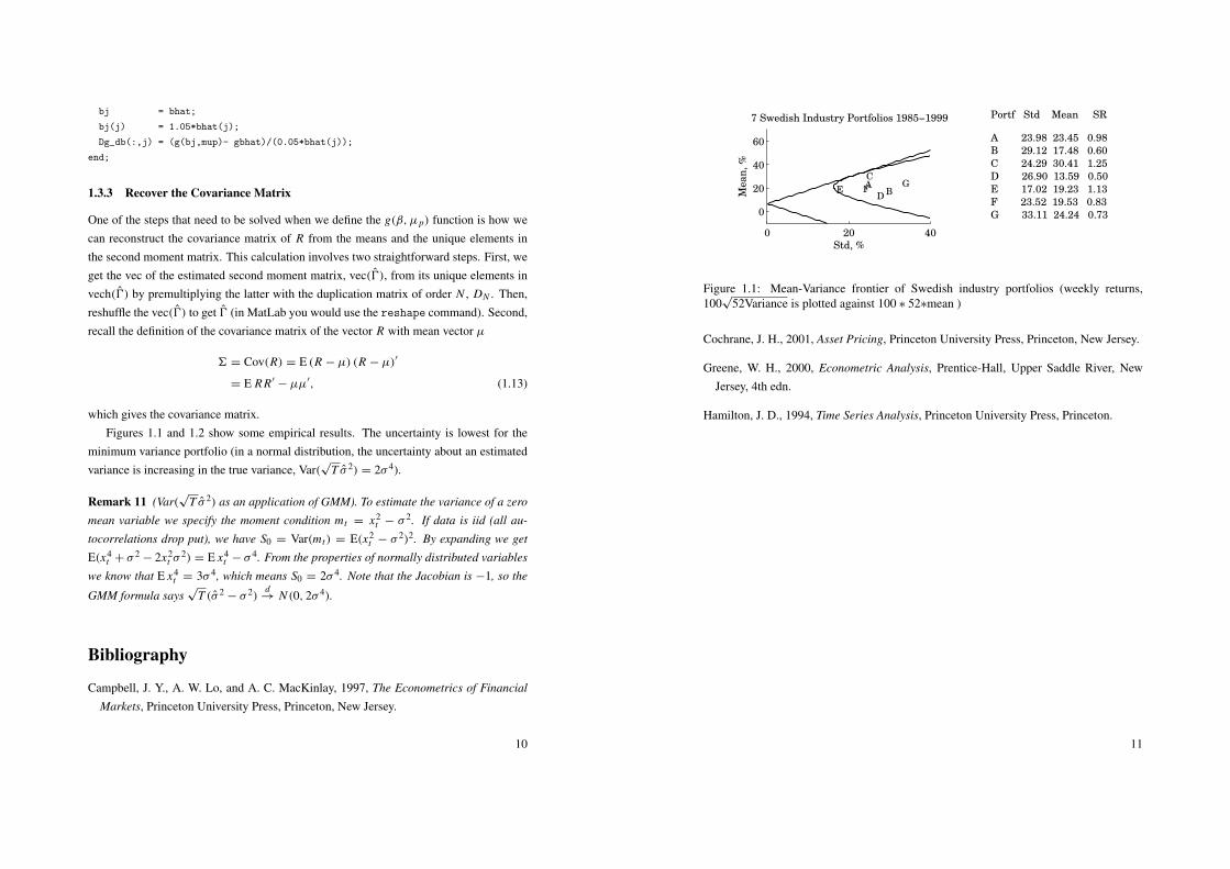
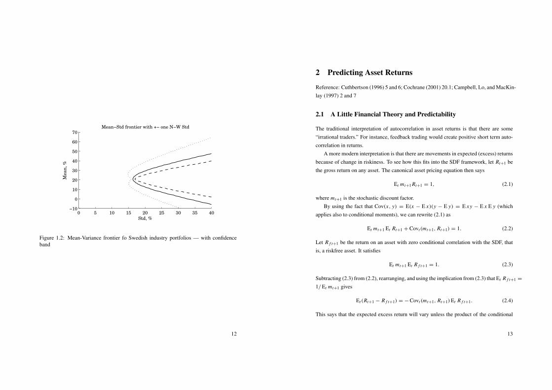
which gives the covariance matrix.Figures 1.1 and 1.2 show some empirical results. The uncertainty is lowest for the

minimum variance portfolio (in a normal distribution, the uncertainty about an estimatedvariance is increasing in the true variance, Var(

√T σ 2) = 2σ 4).

Remark 11 (Var(√

T σ 2) as an application of GMM). To estimate the variance of a zero

mean variable we specify the moment condition mt = x2t − σ 2. If data is iid (all au-

tocorrelations drop put), we have S0 = Var(mt) = E(x2t − σ 2)2. By expanding we get

E(x4t + σ 2

− 2x2t σ

2) = E x4t − σ 4. From the properties of normally distributed variables

we know that E x4t = 3σ 4, which means S0 = 2σ 4. Note that the Jacobian is −1, so the

GMM formula says√

T (σ 2− σ 2)

d→ N (0, 2σ 4).

Bibliography

Campbell, J. Y., A. W. Lo, and A. C. MacKinlay, 1997, The Econometrics of Financial

Markets, Princeton University Press, Princeton, New Jersey.

10

0 20 40

0

20

40

60

7 Swedish Industry Portfolios 1985−1999

Std, %

Mea

n,

%

AB

C

DE F

G

Portf Std Mean SR

A 23.98 23.45 0.98

B 29.12 17.48 0.60

C 24.29 30.41 1.25

D 26.90 13.59 0.50

E 17.02 19.23 1.13

F 23.52 19.53 0.83

G 33.11 24.24 0.73

Figure 1.1: Mean-Variance frontier of Swedish industry portfolios (weekly returns,100

√52Variance is plotted against 100 ∗ 52∗mean )

Cochrane, J. H., 2001, Asset Pricing, Princeton University Press, Princeton, New Jersey.

Greene, W. H., 2000, Econometric Analysis, Prentice-Hall, Upper Saddle River, NewJersey, 4th edn.

Hamilton, J. D., 1994, Time Series Analysis, Princeton University Press, Princeton.

11

0 5 10 15 20 25 30 35 40−10

0

10

20

30

40

50

60

70Mean−Std frontier with +− one N−W Std

Std, %

Mea

n,

%

Figure 1.2: Mean-Variance frontier fo Swedish industry portfolios — with confidenceband

12

2 Predicting Asset Returns

Reference: Cuthbertson (1996) 5 and 6; Cochrane (2001) 20.1; Campbell, Lo, and MacKin-lay (1997) 2 and 7

2.1 A Little Financial Theory and Predictability

The traditional interpretation of autocorrelation in asset returns is that there are some“irrational traders.” For instance, feedback trading would create positive short term auto-correlation in returns.

A more modern interpretation is that there are movements in expected (excess) returnsbecause of change in riskiness. To see how this fits into the SDF framework, let Rt+1 bethe gross return on any asset. The canonical asset pricing equation then says

Et mt+1 Rt+1 = 1, (2.1)

where mt+1 is the stochastic discount factor.By using the fact that Cov(x, y) = E(x − E x)(y − E y) = E xy − E x E y (which

applies also to conditional moments), we can rewrite (2.1) as

Et mt+1 Et Rt+1 + Covt(mt+1, Rt+1) = 1. (2.2)

Let R f t+1 be the return on an asset with zero conditional correlation with the SDF, thatis, a riskfree asset. It satisfies

Et mt+1 Et R f t+1 = 1. (2.3)

Subtracting (2.3) from (2.2), rearranging, and using the implication from (2.3) that Et R f t+1 =

1/Et mt+1 gives

Et(Rt+1 − R f t+1) = − Covt(mt+1, Rt+1)Et R f t+1. (2.4)

This says that the expected excess return will vary unless the product of the conditional

13

covariance and the expected riskfree rate is constant. Note that a changing expected excessreturn is the same as that the future excess return is forecastable. Also note that if the righthand side of (2.4) is constant, then Et Rt+1will move one-for-one with Et R f t+1, so anypredictability in the riskfree rate carries over to the risky return.

We still have an “annoying” Et R f t+1 term in (2.4). Consider nominal returns andsuppose we are in a situation where inflation is expected to be much higher in the future(change of monetary policy regime). Even if the covariance in (2.4) is unchanged (asit would be if this is a deterministic increase in inflation which has no real effects), theexpected excess return changes (as long as the covariance is non-zero) since Et R f t+1

increases. Clearly, this effect disappears if we study real returns instead or if we define theexcess return as Rt+1/R f t+1 instead, as we implicitly do when we analyze continuouslycompounded returns.

For instance, if the SDF and the return are (conditionally) lognormally distributed,then we can arrive at a simple expression for the excess continuously compounded return.Let rt = ln Rt . If ln mt+1 + rt+1 is normally distributed, then we can write the pricingequation as

1 = Et exp(ln mt+1 + rt+1)

= exp[Et ln mt+1 + Et rt+1 + Vart(ln mt+1 + rt+1)/2]. (2.5)

Take logs to get

0 = Et ln mt+1 + Et rt+1 + Vart(ln mt+1)/2 + Vart(rt+1)/2 + Covt(ln mt+1, rt+1) (2.6)

The same applies to the riskfree asset with return r f t+1, except that the covariance withthe SDF is zero. The expected excess (continuously compounded) return is then

Et rt+1 − Et r f t+1 = − Vart(rt+1)/2 + Vart(r f t+1)/2 − Covt(ln mt+1, rt+1). (2.7)

This expression relates the excess return to the second moments, in particular, the covari-ance of the log SDF and the log return.

As an example, consider a simple consumption-based model to start thinking aboutthese issues. Suppose we want to maximize the expected discounted sum of utility

14

Et 6∞

s=0βsu(ct+s). Let Qt be the consumer price index in t . Then, we have

mt+1 =

{β

u′(ct+1)u′(ct )

QtQt+1

if returns are nominal

βu′(ct+1)u′(ct )

if returns are real.(2.8)

This shows that to get a time-varying risk premium in (2.7), the conditional covariance ofthe log marginal utility and the return must change (disregarding the Jensen’s inequalityterms).

2.1.1 Application: Mean-Variance Portfolio Choice with Predictable Returns

If there are non-trivial market imperfections, then predictability can be used to generateeconomic profits. If there are no important market imperfections, then predictability ofexcess returns should be thought of as predictable movements in risk premia. We willtypically focus on this second interpretation.

As a simple example, consider a small mean-variance investor whose preferencesdiffer from the average investor: he is not affected by risk that creates the time vari-ation in expected returns. Suppose he can invest in two assets: a risky asset with re-turn Rt+1 and a risk free asset with return R f and zero variance. The return on theportfolio is Rp,t+1 = αRt+1 + (1 − α)R f . The utility is quadratic in terms of wealth:Et Rp,t+1 − Vart(Rp,t+1)k/2. Substituting gives that the maximization problem is

maxα α Et Rt+1 + (1 − α)R f −k2α2 Vart(Rt+1).

The first order condition is

0 = Et Rt+1 − R f − kαVart(Rt+1) or

α =1k

Et Rt+1 − R f

Vart(Rt+1).

The weight on the risky asset is clearly increasing in the excess return and decreasing inthe variance. If we compare two investors of this type and the same k, but with differentinvestment horizons, then the portfolio weight α is the same if the ratio of the mean andvariance is unchanged by the horizon. This is the case if returns are iid.

To demonstrate the last point note that the two period excess return is approximatelyequal to the sum of two one period returns Rt+1 − R f + Rt+2 − R f . With iid returns the

15

mean of this two period excess return is 2 E(Rt+1 − R f ) and the variance is 2 Var(Rt+1)

since the covariance of the returns is zero. We therefore get

α for 1-period horizon =1k

Et Rt+1 − R f

Vart(Rt+1),

α for 2-period horizon =1k

2 Et(Rt+1 − R f )

2 Vart(Rt+1),

which are the same.With correlated returns we still have the same two period mean, but the variance is

now Var(Rt+1 + Rt+2) = 2 Var(Rt+1) + 2 Cov(Rt+1, Rt+2). This gives the portfolioweight on the risky asset

α for 2 period horizon =1k

2 Et(Rt+1 − R f )

2 Vart(Rt+1)+ 2 Covt(Rt+1, Rt+2).

With mean reversion in prices the covariance is negative, so the weight on the risky assetis larger for the two period horizon than for the one period horizon.

2.2 Empirical U.S. Evidence on Stock Return Predictability

Reference: Bodie, Kane, and Marcus (1999) 12; Cuthbertson (1996) 6.1; and Campbell,Lo, and MacKinlay (1997) 2 and 7; Cochrane (2001) 20.1

The two most common methods for investigating the predictability of stock returns areto calculate autocorrelations and to construct simple dynamic portfolios and see if theyoutperform passive portfolios. The dynamic portfolio could, for instance, be a simplefilter rule that calls for rebalancing once a month by buying (selling) assets which haveincreased (decreased) more than x% the last month. If this portfolio outperforms a passiveportfolio, then this is evidence of some positive autocorrelation (“momentum”) on a one-month horizon. The following points summarize some evidence which seems to hold forboth returns and returns in excess of a riskfree rate (an interest rate).

1. The empirical evidence suggests some, but weak, positive autocorrelation in short

horizon returns (one day up to a month) — probably too little to be able to tradeon. The autocorrelation is stronger for small than for large firms (perhaps no au-tocorrelation at all for weekly or longer returns in large firms). This implies that

16

equally weighted stock indices have larger autocorrelation than value-weighted in-dices. (See Campbell, Lo, and MacKinlay (1997) Table 2.4.)

2. Stock indices have more positive autocorrelation than (most of) the individual stocks:there must be fairly strong cross-autocorrelations across individual stocks. (SeeCampbell, Lo, and MacKinlay (1997) Tables 2.7 and 2.8.)

3. There seems to be negative autocorrelation for multi-year stock returns, for instancein 5-year US returns for 1926-1985. It is unclear what drives this result, how-ever. It could well be an artifact of just a few extreme episodes (Great Depression).Moreover, the estimates are very uncertain as there are very few (non-overlapping)multi-year returns even in a long sample—the results could be just a fluke.

4. The aggregate stock market returns, that is, the returns on a value-weighted stockindex, seem to be forecastable on the medium horizon by various information vari-

ables. In particular, future stock returns seems to be predictable by the currentdividend-price ratio and earnings-price ratios (positively, one to several years), orby the interest rate changes (negatively, up to a year). For instance, the coefficientof determination (usually denoted R2, but should not to be confused with the re-turn used above) for predicted two-year returns on the US stock market on currentdividend-price ratio is around 0.3 for the 1952-1994 sample. (See Campbell, Lo,and MacKinlay (1997) Tables 7.1-2.) This evidence suggests that expected returnsmay very well be time varying and correlated with the business cycle.

5. Even if short-run returns, Rt+1, are fairly hard to forecast, it is often fairly easyto forecast volatility as measured by |Rt+1| or R2

t+1 (for instance, using ARCH orGARCH models). For an example, see Bodie, Kane, and Marcus (1999) Figure13.7. This could possibly be used for dynamic trading strategies on options whichdirectly price volatility. For instance, buying both a call and a put option (a “strad-dle” or a “strangle”), is a bet on a large price movement (in any direction).

6. It is sometimes found that stock prices behave differently in periods with highvolatility than in more normal periods. Granger (1992) reports that the forecast-ing performance is sometimes improved by using different forecasting models forthese two regimes. A simple and straightforward way to estimate a model for peri-

17

1980 1990 20000

20

40

60

80

Stockholm Exchange Index (SIXRX)

Year

SIXRX

T−bill portfolio

1980 1990 2000−10

0

10SIXRX Daily Excess Returns, %

Year

Autocorr 0.11

1980 1990 2000

−10

0

10

SIXRX Weekly Excess Returns, %

Year

Autocorr 0.05

1980 1990 2000

−10

0

10

SIXRX Absolute Weekly Excess Returns, %

Year

Autocorr 0.20

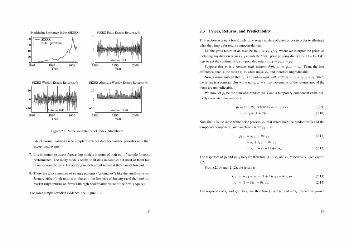
Figure 2.1: Value weighted stock index, Stockholm

ods of normal volatility is to simply throw out data for volatile periods (and otherexceptional events).

7. It is important to assess forecasting models in terms of their out-of-sample forecastperformance. Too many models seems to fit data in-sample, but most of them failin out-of-sample tests. Forecasting models are of no use if they cannot forecast.

8. There are also a number of strange patterns (“anomalies”) like the small-firms-in-January effect (high returns on these in the first part of January) and the book-to-market (high returns on firms with high book/market value of the firm’s equity).

For some simple Swedish evidence, see Figure 2.1.

18

2.3 Prices, Returns, and Predictability

This section sets up a few simple time series models of asset prices in order to illustratewhat they imply for returns autocorrelations.

Let the gross return of an asset be Rt+1 = Pt+1/Pt , where we interpret the prices asincluding any dividends (so Pt+1 equals the “raw” price plus any dividends in t +1). Takelogs to get the continuously compounded return rt+1 = pt+1 − pt .

Suppose that pt is a random walk without drift, pt = pt−1 + εt . Then, the firstdifference, that is, the return rt , is white noise, εt , and therefore unpredictable.

Now, assume instead that pt is a random walk with drift, pt = µ+ pt−1 + εt . Then,the return is a constant plus white noise, µ + εt , so movements of the returns around themean are unpredictable.

We now let pt be the sum of a random walk and a temporary component (with per-fectly correlated innovations)

pt = ut + θεt , where ut = ut−1 + εt (2.9)

= ut−1 + (1 + θ)εt (2.10)

Note that it is the same white noise process, εt , that drives both the random walk and thetemporary component. We can clearly write pt+1 as

pt+1 = ut+1 + θεt+1 (2.11)

= ut + εt+1 + θεt+1

= ut−1 + εt + (1 + θ)εt+1 (2.12)

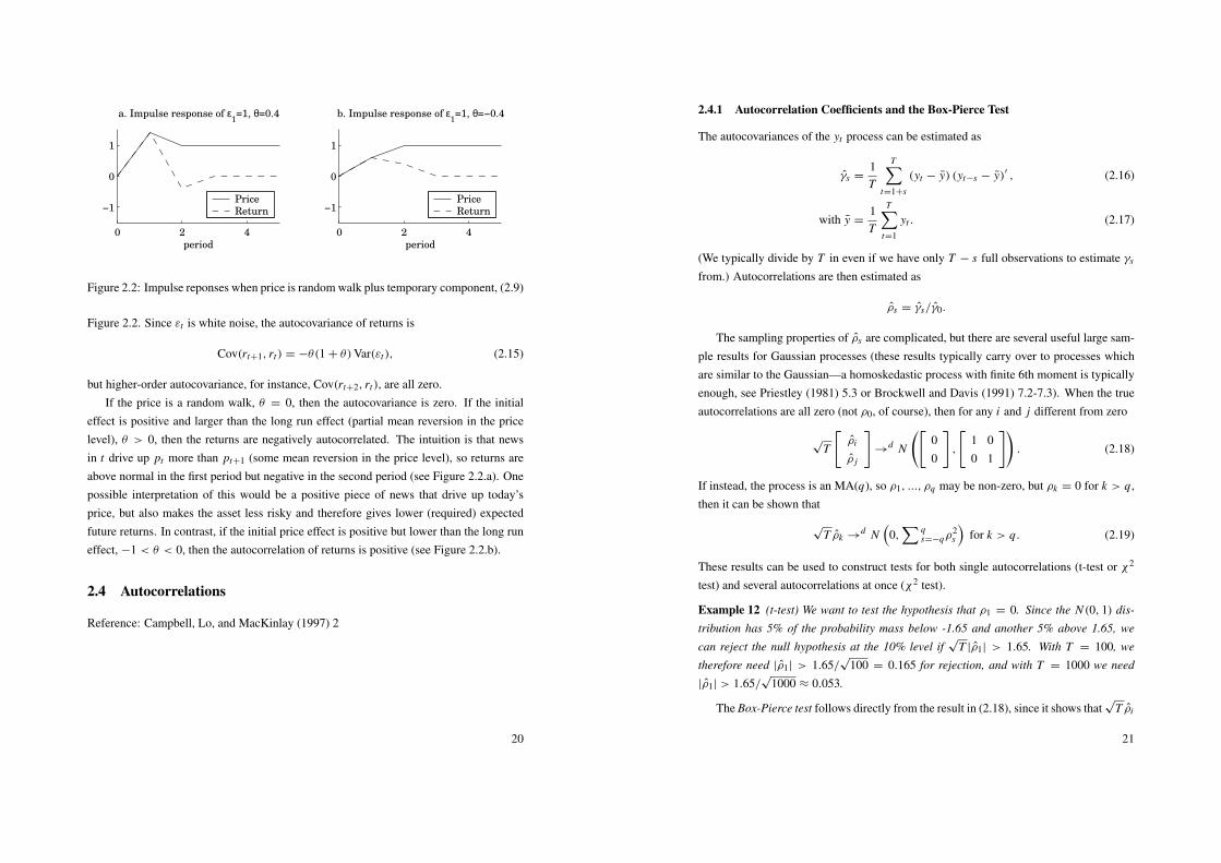
The responses of pt and pt+1 to εt are therefore (1+θ)εt and εt , respectively—see Figure

2.2.From (2.10) and (2.12), the return is

rt+1 = pt+1 − pt = (1 + θ)εt+1 − θεt , so (2.13)

rt = (1 + θ)εt − θεt−1. (2.14)

The responses of rt and rt+1 to εt are therefore (1 + θ)εt and −θεt , respectively—see

19

0 2 4

−1

0

1

a. Impulse response of ε1=1, θ=0.4

period

Price

Return

0 2 4

−1

0

1

b. Impulse response of ε1=1, θ=−0.4

period

Price

Return

Figure 2.2: Impulse reponses when price is random walk plus temporary component, (2.9)

Figure 2.2. Since εt is white noise, the autocovariance of returns is

Cov(rt+1, rt) = −θ(1 + θ)Var(εt), (2.15)

but higher-order autocovariance, for instance, Cov(rt+2, rt), are all zero.If the price is a random walk, θ = 0, then the autocovariance is zero. If the initial

effect is positive and larger than the long run effect (partial mean reversion in the pricelevel), θ > 0, then the returns are negatively autocorrelated. The intuition is that newsin t drive up pt more than pt+1 (some mean reversion in the price level), so returns areabove normal in the first period but negative in the second period (see Figure 2.2.a). Onepossible interpretation of this would be a positive piece of news that drive up today’sprice, but also makes the asset less risky and therefore gives lower (required) expectedfuture returns. In contrast, if the initial price effect is positive but lower than the long runeffect, −1 < θ < 0, then the autocorrelation of returns is positive (see Figure 2.2.b).

2.4 Autocorrelations

Reference: Campbell, Lo, and MacKinlay (1997) 2

20

2.4.1 Autocorrelation Coefficients and the Box-Pierce Test

The autocovariances of the yt process can be estimated as

γs =1T

T∑t=1+s

(yt − y) (yt−s − y)′ , (2.16)

with y =1T

T∑t=1

yt . (2.17)

(We typically divide by T in even if we have only T − s full observations to estimate γs

from.) Autocorrelations are then estimated as

ρs = γs/γ0.

The sampling properties of ρs are complicated, but there are several useful large sam-ple results for Gaussian processes (these results typically carry over to processes whichare similar to the Gaussian—a homoskedastic process with finite 6th moment is typicallyenough, see Priestley (1981) 5.3 or Brockwell and Davis (1991) 7.2-7.3). When the trueautocorrelations are all zero (not ρ0, of course), then for any i and j different from zero

√T

[ρi

ρ j

]→

d N

([00

],

[1 00 1

]). (2.18)

If instead, the process is an MA(q), so ρ1, ..., ρq may be non-zero, but ρk = 0 for k > q,then it can be shown that

√T ρk →

d N(

0,∑ q

s=−qρ2s

)for k > q. (2.19)

These results can be used to construct tests for both single autocorrelations (t-test or χ2

test) and several autocorrelations at once (χ2 test).

Example 12 (t-test) We want to test the hypothesis that ρ1 = 0. Since the N (0, 1) dis-

tribution has 5% of the probability mass below -1.65 and another 5% above 1.65, we

can reject the null hypothesis at the 10% level if√

T |ρ1| > 1.65. With T = 100, we

therefore need |ρ1| > 1.65/√

100 = 0.165 for rejection, and with T = 1000 we need

|ρ1| > 1.65/√

1000 ≈ 0.053.

The Box-Pierce test follows directly from the result in (2.18), since it shows that√

T ρi

21

and√

T ρ j are iid N(0,1) variables. Therefore, the sum of the square of them is distributedas an χ2 variable. The test statistic typically used is

QL = TL∑

s=1

ρ2s →

d χ2L . (2.20)

Example 13 (Box-Pierce) Let ρ1 = 0.165, and T = 100, so Q1 = 100 × 0.1652=

2.72. The 10% critical value of the χ21 distribution is 2.71, so the null hypothesis of no

autocorrelation is rejected.

The choice of lag order in (2.20), L , should be guided by theoretical considerations,but it may also be wise to try different values. There is clearly a trade off: too few lags maymiss a significant high-order autocorrelation, but too many lags can destroy the power ofthe test (as the test statistic is not affected much by increasing L , but the critical valuesincrease).

The main problem with these tests is that the assumptions behind the results in (2.18)may not be reasonable. For instance, data may be heteroskedastic. One way of handlingthis is to make use of the GMM framework.

2.4.2 Box-Pierce as an Application of GMM∗

This section discusses how GMM can be used to test if a series is autocorrelated. Theanalysis focuses on first-order autocorrelation, but it is straightforward to extend it tohigher-order autocorrelation.

Consider a scalar random variable xt with a zero mean (it is easy to extend the analysisto allow for a non-zero mean). Consider the moment conditions

mt(β) =

[x2

t − σ 2

xt xt−1 − ρσ 2

], so m(β) =

1T

T∑t=1

[x2

t − σ 2

xt xt−1 − ρσ 2

], with β =

[σ 2

ρ

].

(2.21)σ 2 is the variance and ρ the first-order autocorrelation so ρσ 2 is the first-order autoco-variance. We want to test if ρ = 0. We could proceed along two different routes: estimateρ and test if it is different from zero or set ρ to zero and then test overidentifying restric-tions. We analyze how the first of these two approaches works when the null hypothesisof ρ = 0 is true.

22

We estimate both σ 2 and ρ by using the moment conditions (2.21) and then test ifρ = 0. To do that we need to calculate the asymptotic variance of ρ (there is little hope ofbeing able to calculate the small sample variance, so we have to settle for the asymptoticvariance as an approximation).

We have an exactly identified system so the weight matrix does not matter—we canthen proceed as if we had used the optimal weighting matrix (all those results apply).

To find the asymptotic covariance matrix of the parameters estimators, we need theprobability limit of the Jacobian of the moments and the covariance matrix of the moments—evaluated at the true parameter values. Let mi (β0) denote the i th element of the m(β)

vector—evaluated at the true parameter values. The probability of the Jacobian is

D0 = plim

[∂m1(β0)/∂σ

2 ∂m1(β0)/∂ρ

∂m2(β0)/∂σ2 ∂m2(β0)/∂ρ

]=

[−1 0−ρ −σ 2

]=

[−1 00 −σ 2

],

(2.22)since ρ = 0 (the true value). Note that we differentiate with respect to σ 2, not σ , sincewe treat σ 2 as a parameter.

The covariance matrix is more complicated. The definition is

S0 = E

[√T

T

T∑t=1

mt(β0)

][√T

T

T∑t=1

mt(β0)

]′

.

Assume that there is no autocorrelation in mt(β0) (which means, among other things, thatvolatility, x2

t , is not autocorrelated). We can then simplify as

S0 = E mt(β0)mt(β0)′.

This assumption is stronger than assuming that ρ = 0, but we make it here in order toillustrate the asymptotic distribution. To get anywhere, we assume that xt is iid N (0, σ 2).In this case (and with ρ = 0 imposed) we get

S0 = E

[x2

t − σ 2

xt xt−1

][x2

t − σ 2

xt xt−1

]′

= E

[(x2

t − σ 2)2 (x2t − σ 2)xt xt−1

(x2t − σ 2)xt xt−1 (xt xt−1)

2

]

=

[E x4

t − 2σ 2 E x2t + σ 4 0

0 E x2t x2

t−1

]=

[2σ 4 0

0 σ 4

]. (2.23)

To make the simplification in the second line we use the facts that E x4t = 3σ 4 if xt ∼

23

N (0, σ 2), and that the normality and the iid properties of xt together imply E x2t x2

t−1 =

E x2t E x2

t−1 and E x3t xt−1 = E σ 2xt xt−1 = 0.

By combining (2.22) and (2.23) we get that

ACov

(√

T

[σ 2

ρ

])=

(D

′

0S−10 D0

)−1

=

[ −1 00 −σ 2

]′ [2σ 4 0

0 σ 4

]−1 [−1 00 −σ 2

]−1

=

[2σ 4 0

0 1

]. (2.24)

This shows the standard expression for the uncertainty of the variance and that the√

T ρ.Since GMM estimators typically have an asymptotic distribution we have

√T ρ →

d

N (0, 1), so we can test the null hypothesis of no first-order autocorrelation by the teststatistic

T ρ2∼ χ2

1 . (2.25)

This is the same as the Box-Pierce test for first-order autocorrelation.This analysis shows that we are able to arrive at simple expressions for the sampling

uncertainty of the variance and the autocorrelation—provided we are willing to makestrong assumptions about the data generating process. In particular, we assumed that datawas iid N (0, σ 2). One of the strong points of GMM is that we could perform similartests without making strong assumptions—provided we use a correct estimator of theasymptotic covariance matrix S0 (for instance, Newey-West).

2.4.3 Autoregressions

An alternative way of testing autocorrelations is to estimate an AR model

yt = a1yt−1 + a2yt−2 + ...+ ap yt−p + εt , (2.26)

and then test if all the coefficients are zero with a χ2 test. This approach is somewhat lessgeneral than the Box-Pierce test, but most stationary time series processes can be wellapproximated by an AR of relatively low order. To account for heteroskedasticity andother problems, it can make sense to estimate the covariance matrix of the parameters by

24

an estimator like Newey-West.

2.4.4 Autoregressions versus Autocorrelations∗

If is straightforward to see the relation between autocorrelations and the AR model whenthe AR model is the true process. This relation is given by the Yule-Walker equations.

For an AR(1), the autoregression coefficient is simply the first autocorrelation coeffi-cient. For an AR(2), yt = a1yt−1 + a2yt−2 + εt , we have Cov(yt , yt)

Cov(yt−1, yt)

Cov(yt−2, yt)

=

Cov(yt , a1yt−1 + a2yt−2 + εt)

Cov(yt−1, a1yt−1 + a2yt−2 + εt)

Cov(yt−2, a1yt−1 + a2yt−2 + εt)

=

a1 Cov(yt , yt−1)+ a2 Cov(yt , yt−2)+ Cov(yt , εt)

a1 Cov(yt−1, yt−1)+ a2 Cov(yt−1, yt−2)

a1 Cov(yt−2, yt−1)+ a2 Cov(yt−2, yt−2)

, or

γ0

γ1

γ2

=

a1γ1 + a2γ2 + Var(εt)

a1γ0 + a2γ1

a1γ1 + a2γ0

. (2.27)

To transform to autocorrelation, divide through by γ0. The last two equations are then[ρ1

ρ2

]=

[a1 + a2ρ1

a1ρ1 + a2

]or

[ρ1

ρ2

]=

[a1/ (1 − a2)

a21/ (1 − a2)+ a2

]. (2.28)

If we know the parameters of the AR(2) model (a1, a2, and Var(εt)), then we can solvefor the autocorrelations. Alternatively, if we know the autocorrelations, then we can solvefor the autoregression coefficients. This demonstrates that testing that all the autocorre-lations are zero is essentially the same as testing if all the autoregressive coefficients arezero. Note, however, that the transformation is non-linear, which may make a differencein small samples.

2.4.5 Variance Ratios

The 2-period variance ratio is the ratio of Var(yt +yt−1) to 2 Var(yt). To simplify notation,let yt have a zero mean (or be demeaned), so Cov(yt , yt−s) = E yt yt−s , with short hand

25

notation γs . We can then write the variance ratio as

V R2 =E(yt + yt−1)

2

2 E y2t

(2.29)

=E y2

t + E y2t−1 + E yt yt−1 + E yt−1yt

2 E y2t

=γ0 + γ0 + γ1 + γ−1

2γ0. (2.30)

Let ρs = γs/γ0 be the sth autocorrelation. We can then write (2.30) as

=12(ρ−1 + 2 + ρ1) (2.31)

= 1 + ρ1, (2.32)

where we exploit the fact that the autocorrelation (and autocovariance) function is sym-metric around zero, so ρ−s = ρs (and γ−s = γs). Note, however, that this does not holdfor cross autocorrelations (Cov(xt , yt−s) 6= Cov(xt−s, yt)).

It is clear from (2.32) that if yt is not serially correlated, then the variance ratio is unity;a value above one indicates positive serial correlation and a value below one indicatesnegative serial correlation.

We can also consider longer variance rations, where we sum q observations in thenumerator and then divide by q Var(yt). To see the pattern of what happens, considerq = 3 and assume that yt has a zero mean so we can use second moments for covariances.In that case, the numerator Var(yt + yt−1 + yt−2) = E(yt + yt−1 + yt−2)(yt + yt−1 + yt−2)

is(E y2

t + E yt yt−1 + E yt yt−2

)︸ ︷︷ ︸

γ0+γ1+γ2

+

(E yt−1yt + E y2

t−1 + E yt−1yt−2

)︸ ︷︷ ︸

γ−1+γ0+γ1

+

(E yt−2yt + E yt−2yt−1 + E y2

t−2

)︸ ︷︷ ︸

γ−2+γ−1+γ0

= γ−2 + 2γ−1 + 3γ0 + 2γ1 + γ2. (2.33)

It can be noted that the (numerator of the) variance ratios are fairly similar to the uncer-tainty of a sample average.

26

The variance ratio is therefore

V R3 =1

3γ0(γ−2 + 2γ−1 + 3γ0 + 2γ1 + γ2)

=13(ρ−2 + 2ρ−1 + 3 + 2ρ1 + ρ2) . (2.34)

Comparing V R2 in (2.31) and V R3 in (2.34) suggests that V Rq is a similar weightedaverage of autocorrelations, where the weights are tent-shaped (1 at lag 0, 1/q at lag q−1,and zero at lag q and beyond). In fact, it can be shown that we have

V Rq =

Var(∑q−1

s=0 yt−s

)q Var(yt)

(2.35)

=

q−1∑s=−(q−1)

(1 −

|s|q

)ρs or (2.36)

= 1 + 2q−1∑s=1

(1 −

sq

)ρs . (2.37)

Note that we could equally well let the summation in (2.36) run from −q to q since theweight 1 − |s| /q, is zero for that lag. The same holds for (2.37).

It is immediate that no autocorrelation means that V Rq = 1 for all q. If all autocorre-lations are non-positive, ρs ≤ 0, then V Rq ≤ 1, and vice versa.

Example 14 (Variance ratio of an AR(1)) When yt = ayt−1 + εt where εt is iid white

noise, then

V R2 =12

a + 1 +12

a = 1 + a and

V R3 =13

a2+

23

a + 1 +23

a +13

a2= 1 +

43

a +23

a2

V R4 =14

a3+

24

a2+

34

a + 1 +34

a +24

a2+

14

a3= 1 +

32

a + a2+

12

a3.

See Figure 2.3 for a numerical example.

The estimation of V Rq is done by replacing the population variances in (2.35) withthe sample variances, or the autocorrelations in (2.37) by the sample autocorrelations.

The sampling distribution of V Rq under the null hypothesis that there is no autocor-relation follows directly from the sampling distribution of the autocorrelation coefficient.

27

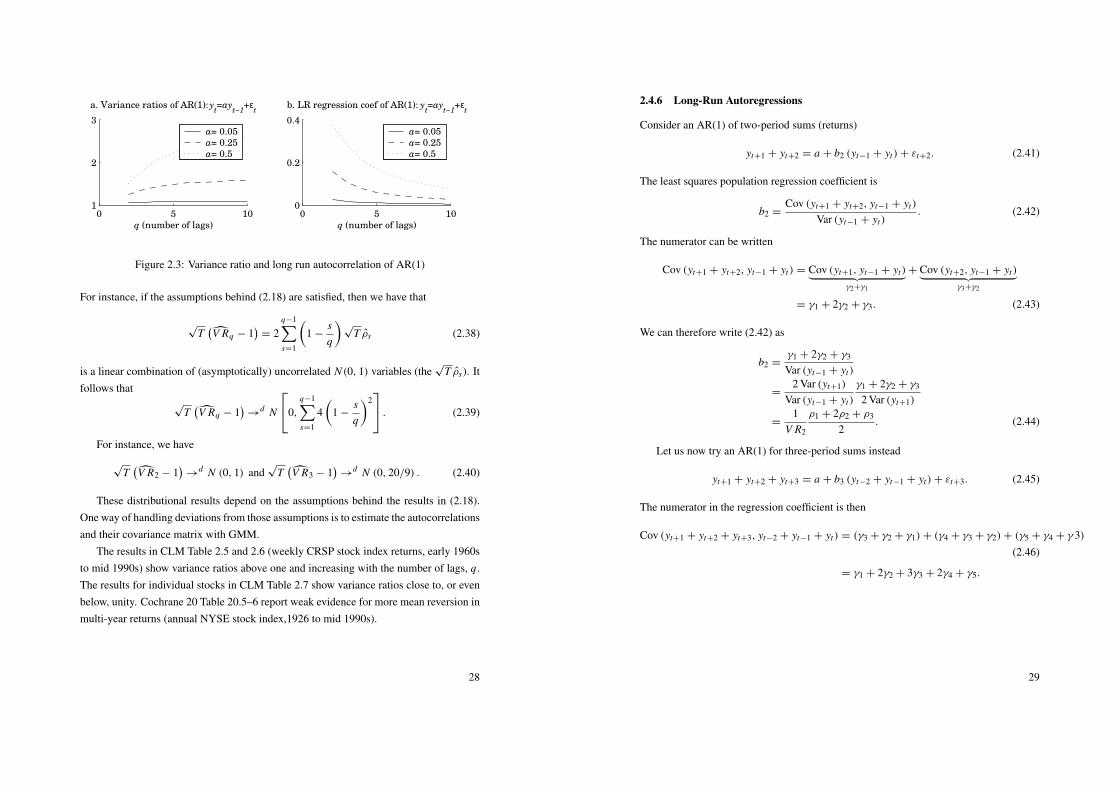
0 5 101

2

3

a. Variance ratios of AR(1): yt=ay

t−1+ε

t

q (number of lags)

a= 0.05

a= 0.25

a= 0.5

0 5 100

0.2

0.4

b. LR regression coef of AR(1): yt=ay

t−1+ε

t

q (number of lags)

a= 0.05

a= 0.25

a= 0.5

Figure 2.3: Variance ratio and long run autocorrelation of AR(1)

For instance, if the assumptions behind (2.18) are satisfied, then we have that

√T(V Rq − 1

)= 2

q−1∑s=1

(1 −

sq

)√

T ρs (2.38)

is a linear combination of (asymptotically) uncorrelated N (0, 1) variables (the√

T ρs). Itfollows that

√T(V Rq − 1

)→

d N

0,q−1∑s=1

4(

1 −sq

)2 . (2.39)

For instance, we have

√T(V R2 − 1

)→

d N (0, 1) and√

T(V R3 − 1

)→

d N (0, 20/9) . (2.40)

These distributional results depend on the assumptions behind the results in (2.18).One way of handling deviations from those assumptions is to estimate the autocorrelationsand their covariance matrix with GMM.

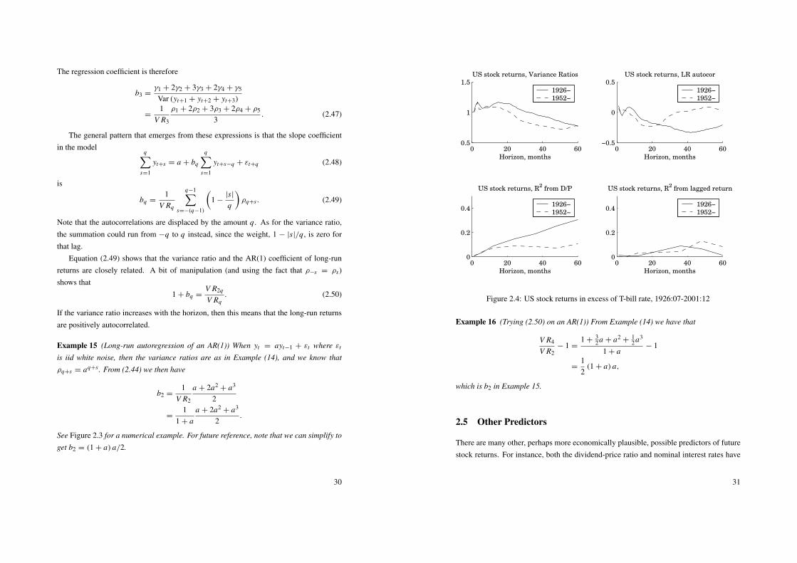
The results in CLM Table 2.5 and 2.6 (weekly CRSP stock index returns, early 1960sto mid 1990s) show variance ratios above one and increasing with the number of lags, q.The results for individual stocks in CLM Table 2.7 show variance ratios close to, or evenbelow, unity. Cochrane 20 Table 20.5–6 report weak evidence for more mean reversion inmulti-year returns (annual NYSE stock index,1926 to mid 1990s).

28

2.4.6 Long-Run Autoregressions

Consider an AR(1) of two-period sums (returns)

yt+1 + yt+2 = a + b2 (yt−1 + yt)+ εt+2. (2.41)

The least squares population regression coefficient is

b2 =Cov (yt+1 + yt+2, yt−1 + yt)

Var (yt−1 + yt). (2.42)

The numerator can be written

Cov (yt+1 + yt+2, yt−1 + yt) = Cov (yt+1, yt−1 + yt)︸ ︷︷ ︸γ2+γ1

+ Cov (yt+2, yt−1 + yt)︸ ︷︷ ︸γ3+γ2

= γ1 + 2γ2 + γ3. (2.43)

We can therefore write (2.42) as

b2 =γ1 + 2γ2 + γ3

Var (yt−1 + yt)

=2 Var (yt+1)

Var (yt−1 + yt)

γ1 + 2γ2 + γ3

2 Var (yt+1)

=1

V R2

ρ1 + 2ρ2 + ρ3

2. (2.44)

Let us now try an AR(1) for three-period sums instead

yt+1 + yt+2 + yt+3 = a + b3 (yt−2 + yt−1 + yt)+ εt+3. (2.45)

The numerator in the regression coefficient is then

Cov (yt+1 + yt+2 + yt+3, yt−2 + yt−1 + yt) = (γ3 + γ2 + γ1)+ (γ4 + γ3 + γ2)+ (γ5 + γ4 + γ 3)(2.46)

= γ1 + 2γ2 + 3γ3 + 2γ4 + γ5.

29

The regression coefficient is therefore

b3 =γ1 + 2γ2 + 3γ3 + 2γ4 + γ5

Var (yt+1 + yt+2 + yt+3)

=1

V R3

ρ1 + 2ρ2 + 3ρ3 + 2ρ4 + ρ5

3. (2.47)

The general pattern that emerges from these expressions is that the slope coefficientin the model

q∑s=1

yt+s = a + bq

q∑s=1

yt+s−q + εt+q (2.48)

is

bq =1

V Rq

q−1∑s=−(q−1)

(1 −

|s|q

)ρq+s . (2.49)

Note that the autocorrelations are displaced by the amount q. As for the variance ratio,the summation could run from −q to q instead, since the weight, 1 − |s|/q , is zero forthat lag.

Equation (2.49) shows that the variance ratio and the AR(1) coefficient of long-runreturns are closely related. A bit of manipulation (and using the fact that ρ−s = ρs)shows that

1 + bq =V R2q

V Rq. (2.50)

If the variance ratio increases with the horizon, then this means that the long-run returnsare positively autocorrelated.

Example 15 (Long-run autoregression of an AR(1)) When yt = ayt−1 + εt where εt

is iid white noise, then the variance ratios are as in Example (14), and we know that

ρq+s = aq+s . From (2.44) we then have

b2 =1

V R2

a + 2a2+ a3

2

=1

1 + aa + 2a2

+ a3

2.

See Figure 2.3 for a numerical example. For future reference, note that we can simplify to

get b2 = (1 + a) a/2.

30

0 20 40 600.5

1

1.5US stock returns, Variance Ratios

Horizon, months

1926−

1952−

0 20 40 60−0.5

0

0.5US stock returns, LR autocor

Horizon, months

1926−

1952−

0 20 40 600

0.2

0.4

US stock returns, R2 from D/P

Horizon, months

1926−

1952−

0 20 40 600

0.2

0.4

US stock returns, R2 from lagged return

Horizon, months

1926−

1952−

Figure 2.4: US stock returns in excess of T-bill rate, 1926:07-2001:12

Example 16 (Trying (2.50) on an AR(1)) From Example (14) we have that

V R4

V R2− 1 =

1 +32a + a2

+12a3

1 + a− 1

=12(1 + a) a,

which is b2 in Example 15.

2.5 Other Predictors

There are many other, perhaps more economically plausible, possible predictors of futurestock returns. For instance, both the dividend-price ratio and nominal interest rates have

31

been used to predict long-run returns, and lagged short-run returns on other assets havebeen used to predict short-run returns.

2.5.1 Lead-Lags

Reference: Campbell, Lo, and MacKinlay (1997) 2Stock indices have more positive autocorrelation than (most) the individual stocks:

there should therefore be fairly strong cross-autocorrelations across individual stocks.(See Campbell, Lo, and MacKinlay (1997) Tables 2.7 and 2.8.) Indeed, this is also whatis found in US data where weekly returns of large size stocks forecast weekly returns ofsmall size stocks.

2.5.2 Prices and Dividends: Accounting Identity

Reference: Campbell, Lo, and MacKinlay (1997) 7 and Cochrane (2001) 20.1.The gross return, Rt+1, is defined as

Rt+1 =Dt+1 + Pt+1

Pt, so Pt =

Dt+1 + Pt+1

Rt+1. (2.51)

Substituting for Pt+1 (and then Pt+2, ...) gives

Pt =Dt+1

Rt+1+

Dt+2

Rt+1 Rt+2+

Dt+3

Rt+1 Rt+2 Rt+3+ . . . (2.52)

=

∞∑j=1

Dt+ j∏ jk=1 Rt+k

, (2.53)

provided the discounted value of Pt+ j goes to zero as j → ∞. This is simply an ac-counting identity. It is clear that a high price in t must lead to low future returns and/orhigh future dividends—which (by rational expectations) also carry over to expectationsof future returns and dividends.

It is sometimes more convenient to analyze the price-dividend ratio. Dividing (2.52)

32

and (2.53) by Dt gives

Pt

Dt=

1Rt+1

Dt+1

Dt+

1Rt+1 Rt+2

Dt+2

Dt+1

Dt+1

Dt+

1Rt+1 Rt+2 Rt+3

Dt+3

Dt+2

Dt+2

Dt+1

Dt+1

Dt+ . . .

(2.54)

=

∞∑j=1

j∏k=1

Dt+k/Dt+k−1

Rt+k. (2.55)

As with (2.53) it is just an accounting identity. It must therefore also hold in expectations.Since expectations are good (the best?) predictors of future values, we have the impli-cation that the asset price should predict a discounted sum of future dividends, (2.53),and that the price-dividend ratio should predict a discounted sum of future changes individends.

2.5.3 Prices and Dividends: Approximating the Accounting Identity

We now log-linearize the accounting identity (2.55) in order to tie it more closely to the(typically linear) econometrics methods for detecting forecastability.

Rewrite (2.51) as

Rt+1 =Dt+1 + Pt+1

Pt=

Pt+1

Pt

(1 +

Dt+1

Pt+1

)or in logs

rt+1 = pt+1 − pt + ln[1 + exp(dt+1 − pt+1)

]. (2.56)

Make a first order Taylor approximation of the last term around a steady state value ofdt+1 − pt+1, denoted d − p,

ln[1 + exp(dt+1 − pt+1)

]≈ ln

[1 + exp(d − p)

]+

exp(d − p)

1 + exp(d − p)

[dt+1 − pt+1 −

(d − p

)]≈ constant + (1 − ρ) (dt+1 − pt+1) , (2.57)

where ρ = 1/[1 + exp(d − p)] = 1/[1 + D/P)]. If the average dividend-price ratio is4%, then ρ = 1/1.04 ≈ 0.96.

33

We use (2.57) in (2.56) and forget about the constant. The result is

rt+1 ≈ pt+1 − pt + (1 − ρ) (dt+1 − pt+1)

= ρpt+1 − pt + (1 − ρ) dt+1, (2.58)

where 0 < ρ < 1.Add and subtract dt from the right hand side and rearrange

rt+1 ≈ ρ (pt+1 − dt+1)− (pt − dt)+ (dt+1 − dt) , or (2.59)

pt − dt ≈ ρ (pt+1 − dt+1)+ (dt+1 − dt)− rt+1 (2.60)

This is a (forward looking, unstable) difference equation, which we can solve recursivelyforward. Provided lims→∞ ρs(pt+s − dt+s) = 0, the solution is

pt − dt ≈

∞∑s=0

ρs[(dt+1+s − dt+s)− rt+1+s]. (2.61)

(Trying to solve for the log price level instead of the log price-dividend ratio is problematicsince the condition lims→∞ ρs pt+s = 0 may not be satisfied.) As before, a high price-dividend ratio must imply future dividend growth and/or low future returns.

In the exact solution (2.54), dividends and returns which are closer to the present showup more times than dividends and returns far in the future. In the approximation (2.61),this is captured by giving a higher weight (higher ρs).

2.5.4 Dividend-Price Ratio as a Predictor

One of the most successful attempts to forecast long-run return is by using the dividend-price ratio

q∑s=1

rt+s = α + βq(dt − pt)+ εt+q . (2.62)

For instance, CLM Table 7.1, report R2 values from this regression which are close tozero for monthly returns, but they increase to 0.4 for 4-year returns (US, value weightedindex, mid 1920s to mid 1990s).

By comparing with (2.61), we see that the dividend-ratio in (2.62) is only asked topredict a finite (unweighted) sum of future returns—dividend growth is disregarded. We

34

should therefore expect (2.62) to work particularly well if the horizon is long (high q) andif dividends are stable over time.

From (2.61) we get that

Var(pt − dt) ≈ Cov

(pt − dt ,

∞∑s=0

ρs (dt+1+s − dt+s)

)− Cov

(pt − dt ,

∞∑s=0

ρsrt+1+s

),

(2.63)which shows that the variance of the price-dividend ratio can be decomposed into thecovariance of price-dividend ratio with future dividend change minus the covariance ofprice-dividend ratio with future returns. This expression highlights that if pt − dt is notconstant, then it must forecast dividend growth and/or returns.

The evidence in Cochrane suggests that pt − dt does not forecast future dividendgrowth, so that forecastability of future returns explains the variability in the dividend-price ratio. This fits very well into the findings of the R2 of (2.62). To see that, recall thefollowing fact.

Remark 17 (R2 from a least squares regression) Let the least squares estimate of β in

yt = x ′tβ0 + ut be β. The fitted values yt = x ′

t β. If the regression equation includes a

constant, then R2= Corr

(yt , yt

)2. In a simple regression where yt = a+bxt +ut , where

xt is a scalar, R2= Corr (yt , xt)

2.

2.5.5 Predictability but No Autocorrelation

The evidence for US stock returns is that long-run returns may perhaps be predicted byusing dividend-price ratio or interest rates, but that the long-run autocorrelations are weak(long run US stock returns appear to be “weak-form efficient” but not “semi-strong effi-cient”). Both CLM 7.1.4 and Cochrane 20.1 use small models for discussing this case.The key in these discussions is to make changes in dividends unforecastable, but let the re-turn be forecastable by some state variable (Et dt+1+s −Et dt+s = 0 and Et rt+1 = r +xt ),but in such a way that there is little autocorrelation in returns. By taking expectations of(2.61) we see that price-dividend will then reflect expected future returns and therefore beuseful for forecasting.

35

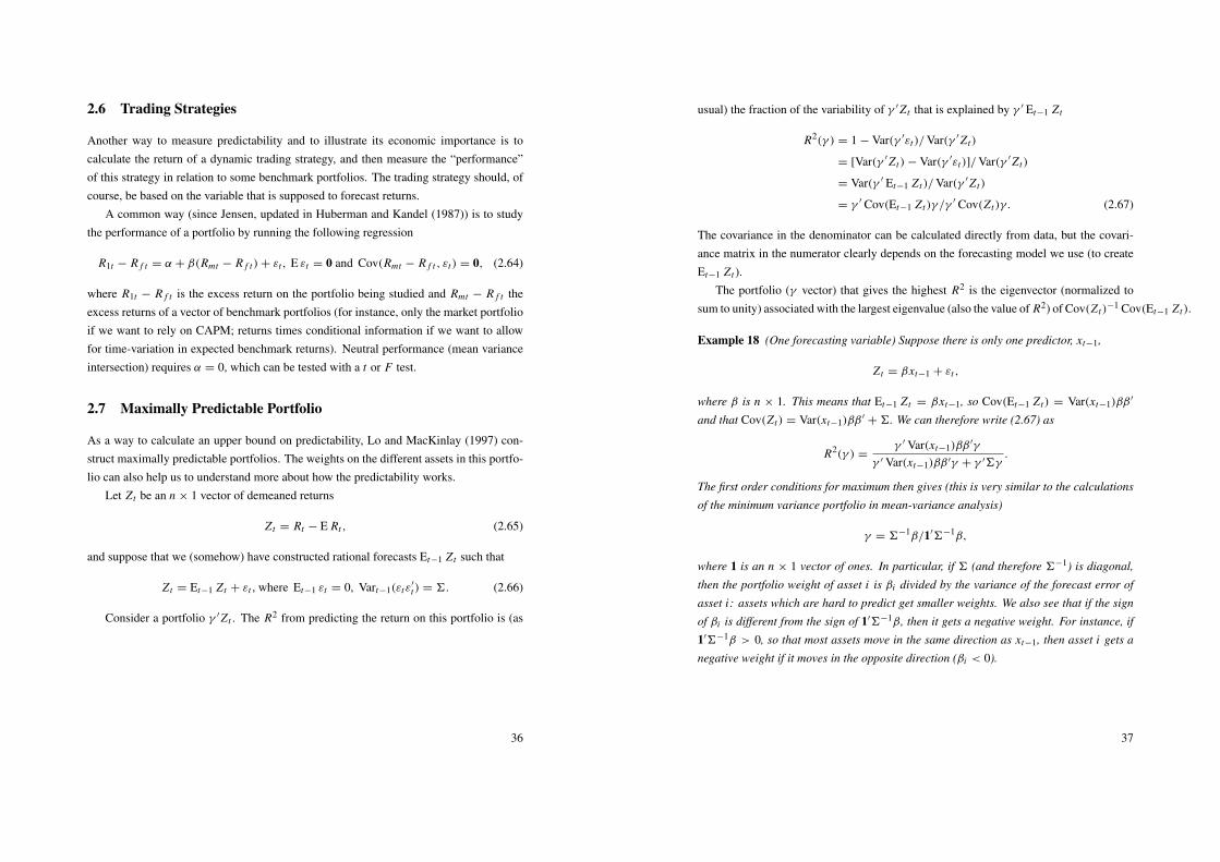
2.6 Trading Strategies

Another way to measure predictability and to illustrate its economic importance is tocalculate the return of a dynamic trading strategy, and then measure the “performance”of this strategy in relation to some benchmark portfolios. The trading strategy should, ofcourse, be based on the variable that is supposed to forecast returns.

A common way (since Jensen, updated in Huberman and Kandel (1987)) is to studythe performance of a portfolio by running the following regression

R1t − R f t = α + β(Rmt − R f t)+ εt , E εt = 0 and Cov(Rmt − R f t , εt) = 0, (2.64)

where R1t − R f t is the excess return on the portfolio being studied and Rmt − R f t theexcess returns of a vector of benchmark portfolios (for instance, only the market portfolioif we want to rely on CAPM; returns times conditional information if we want to allowfor time-variation in expected benchmark returns). Neutral performance (mean varianceintersection) requires α = 0, which can be tested with a t or F test.

2.7 Maximally Predictable Portfolio

As a way to calculate an upper bound on predictability, Lo and MacKinlay (1997) con-struct maximally predictable portfolios. The weights on the different assets in this portfo-lio can also help us to understand more about how the predictability works.

Let Z t be an n × 1 vector of demeaned returns

Z t = Rt − E Rt , (2.65)

and suppose that we (somehow) have constructed rational forecasts Et−1 Z t such that

Z t = Et−1 Z t + εt , where Et−1 εt = 0, Vart−1(εtε′

t) = 6. (2.66)

Consider a portfolio γ ′Z t . The R2 from predicting the return on this portfolio is (as

36

usual) the fraction of the variability of γ ′Z t that is explained by γ ′ Et−1 Z t

R2(γ ) = 1 − Var(γ ′εt)/Var(γ ′Z t)

= [Var(γ ′Z t)− Var(γ ′εt)]/Var(γ ′Z t)

= Var(γ ′ Et−1 Z t)/Var(γ ′Z t)

= γ ′ Cov(Et−1 Z t)γ /γ′ Cov(Z t)γ. (2.67)

The covariance in the denominator can be calculated directly from data, but the covari-ance matrix in the numerator clearly depends on the forecasting model we use (to createEt−1 Z t ).

The portfolio (γ vector) that gives the highest R2 is the eigenvector (normalized tosum to unity) associated with the largest eigenvalue (also the value of R2) of Cov(Z t)

−1 Cov(Et−1 Z t).

Example 18 (One forecasting variable) Suppose there is only one predictor, xt−1,

Z t = βxt−1 + εt ,

where β is n × 1. This means that Et−1 Z t = βxt−1, so Cov(Et−1 Z t) = Var(xt−1)ββ′

and that Cov(Z t) = Var(xt−1)ββ′+6. We can therefore write (2.67) as

R2(γ ) =γ ′ Var(xt−1)ββ

′γ

γ ′ Var(xt−1)ββ ′γ + γ ′6γ.

The first order conditions for maximum then gives (this is very similar to the calculations

of the minimum variance portfolio in mean-variance analysis)

γ = 6−1β/1′6−1β,

where 1 is an n × 1 vector of ones. In particular, if 6 (and therefore 6−1) is diagonal,

then the portfolio weight of asset i is βi divided by the variance of the forecast error of

asset i: assets which are hard to predict get smaller weights. We also see that if the sign

of βi is different from the sign of 1′6−1β, then it gets a negative weight. For instance, if

1′6−1β > 0, so that most assets move in the same direction as xt−1, then asset i gets a

negative weight if it moves in the opposite direction (βi < 0).

37

A Testing Rational Expectations∗

Reference: Cuthbertson (1996) 5.4

A.0.1 Rational Expectations and Survey Data

If we have survey data, then we can perform a direct test of rational expectations. Considerthe scalar variable xt and suppose we have survey data on the expected value in the nextperiod, Ep

t Dt+1. If expectations are rational, then the forecast error Dt+1 − Ept Dt+1

should be unforecastable. In particular, if zt is known in t , then

E[(Dt+1 − Ept Dt+1)zt ] = 0. (A.1)

This implies that a regression of the forecast errors on any information known in t mustgive only zero coefficients. Of course, zt could be a constant so (A.1) says that the meanforecast error should be zero. In practice, this means running the regression

Dt+1 − Ept Dt+1 = α′Z t + εt+1, (A.2)

where zt ∈ Z t and testing if all coefficients (α) are zero.There are, of course, a few problems with this approach. First, samples can be small

(that is always the curse of applied statistics), so that the sample estimate of (A.1) isdifferent from zero by mere chance—in particularly if there was a major surprise duringthe sample.

Second, the survey respondents may not be the agents that we are most interested in.For instance, suppose the traders actually believe in the efficient market hypothesis at thatthe current stock price equals traders’ expectations of future stock prices. However, asurvey of stock price expectations, even if sent to firms on the financial market, is morelikely to be answered by financial forecasters/analysts—who may have other expectations.Third, even if the survey respondents are the persons we are interested in (or are likelyto share the beliefs with those that we care about), they may choose to miss-report forstrategic reasons.

38

A.0.2 Orthogonality Restrictions and Cross-Equation Restrictions

Suppose we are (somehow) equipped with the correct model, which gives an expressionfor the expected value

Ept Dt+1 = γ ′xt . (A.3)

For instance, Dt could be an asset return, so this would be a model of expected assetreturns. In the crudest case, it could be that the expected asset return equals the risk freeinterest rate plus a constant risk premium.

We can test the rational expectations hypothesis by using this expression in (A.1)-(A.2), that is, by an orthogonality test. If we know the values of γ , then we can simplycalculate a time series of Ep

t Dt+1 and then use it in (A.2). If we do not know γ (but arestill sure about which variables that belong to the model), then we can combine (A.3) and(A.2) to get the regression equation

Dt+1 = γ ′xt + α′Z t + εt+1, (A.4)

and test if all elements in α are zero.This approach can also suffer from the small sample problem, but the really serious

problem is probably the specification of the forecasting model. Suppose (A.3) is wrong,and that one of the variables in Z t belongs to the asset pricing model: (A.2) and (A.4) arethen likely to reject the null hypothesis of rational expectations.

A.0.3 Cross-Equation Restrictions

Consider an asset price that is a discounted value of a stream of future “dividends.” Inthe simplest case, the discounting factor (expected return) is a constant, β, and the asset“dies” after the next dividend. In this case, the asset price is

Pt = β Ept Dt+1. (A.5)

Suppose we have data on a time sequence of such assets (with constant discount factor).Suppose also that the true forecasting equation for Dt+1 is

Dt+1 = γ1x1t + γ2x2t + υt+1, so E Dt+1 = γ1x1t + γ2x2t , (A.6)

39

where we let xt be a 2 × 1 vector to simplify the exposition. The only difference between(A.3) and (A.6) is that the latter is the true data generating process, whereas the latter isan equation for how the agents on the financial market form their expectations. If theseare identical, that is, if expectations are rational, then we can use (A.6) in (A.5) to get

Pt = βγ1x1t + βγ2x2t + ut (A.7)

= δ1x1t + δ2x2t + ut . (A.8)

We could estimate the four coefficients in (A.8) and (A.6): γ1, γ2, δ1, and δ2. Note,however, that there are only three “deep” parameters: β, γ1, and γ2, so there are cross-equation ((A.8) and (A.6)) restrictions that can be imposed and tested. The simplest wayto do that is to use GMM and use the theoretical equations (A.6) and -(A.7) to specify thefollowing moment conditions

mt =1T

T∑t=1

(Dt+1 − γ1x1t − γ2x2t) x1t

(Dt+1 − γ1x1t − γ2x2t) x2t

(Pt − βγ1x1t − βγ2x2t) x1t

(Pt − βγ1x1t − βγ2x2t) x2t

. (A.9)

There are four moment conditions, but only three parameters. We can therefore use GMMto estimate the parameters and then test if the single overidentifying restriction is satisfied.

Bibliography

Bodie, Z., A. Kane, and A. J. Marcus, 1999, Investments, Irwin/McGraw-Hill, Boston,4th edn.

Brockwell, P. J., and R. A. Davis, 1991, Time Series: Theory and Methods, SpringerVerlag, New York, second edn.

Campbell, J. Y., A. W. Lo, and A. C. MacKinlay, 1997, The Econometrics of Financial

Markets, Princeton University Press, Princeton, New Jersey.

Cochrane, J. H., 2001, Asset Pricing, Princeton University Press, Princeton, New Jersey.

Cuthbertson, K., 1996, Quantitative Financial Economics, Wiley, Chichester, England.

40

Granger, C. W. J., 1992, “Forecasting Stock Market Prices: Lessons for Forecasters,”International Journal of Forecasting, 8, 3–13.

Huberman, G., and S. Kandel, 1987, “Mean-Variance Spanning,” Journal of Finance, 42,873–888.

Lo, A. W., and A. C. MacKinlay, 1997, “Maximizing Predictability in the Stock and BondMarkets,” Macroeconomic Dynamics, 1, 102–134.

Priestley, M. B., 1981, Spectral Analysis and Time Series, Academic Press.

41

3 Linear Factor Models

3.1 Testing CAPM (Single Excess Return Factor)

Reference: Cochrane (2001) 12.1; Campbell, Lo, and MacKinlay (1997) 5

3.1.1 One Asset at a Time—Traditional ML/LS Approach (iid Returns)

Let Rei t = Ri t − R f t be the excess return on asset i in excess over the riskfree asset, and

let ft = Rmt − R f t be the excess return on the market portfolio. CAPM with a riskfreereturn says that αi = 0 in

Rei t = α + β ft + εi t , where E εi t = 0 and Cov( ft , εi t) = 0. (3.1)

See Cochrane (2001) 9.1 for several derivations of CAPM.This has often been investigated by estimating with LS, and then testing (with a t-test)

if the intercept is zero. If the disturbance is iid normally distributed, then this approach isthe ML approach.

This test of CAPM can be given two interpretations. If we assume that Rmt is thecorrect benchmark, then it is a test of whether asset Ri t is correctly priced. Alternatively,if we assume that Ri t is correctly priced, then it is a test of the mean-variance efficiencyof Rmt (compare the Roll critique).

Remark 19 Consider the regression equation yt = x ′tb0 + ut . With iid errors that are

independent of all regressors (also across observations), the LS estimator, bLs , is asymp-

totically distributed as

√T (bLs − b0)

d→ N (0, σ 26−1

xx ), where σ 2= E u2

t and 6xx = E1T6T

t=1xt x ′

t .

When the regressors are just a constant (equal to one) and one variable regressor, ft , so

42

xt = [1, ft ]′, then we have

6xx = E1T∑T

t=1xt x ′

t = E1T∑T

t=1

[1 ft

ft f 2t

]=

[1 E ft

E ft E f 2t

], so

σ 26−1xx =

σ 2

E f 2t − (E ft)2

[E f 2

t − E ft

− E ft 1

]=

σ 2

Var( ft)

[Var( ft)+ (E ft)

2− E ft

− E ft 1

].

(In the last line we use Var( ft) = E f 2t − (E ft)

2.)

This remark fits well with the CAPM regression (3.1). The variance of the interceptestimator is therefore

Var[√

T (α − α0)] =

{1 +

(E ft)2

Var ( ft)

}Var(εi t) (3.2)

= [1 + (S R f )2] Var(εi t), (3.3)

where S R f is the Sharpe ratio of the market portfolio (recall: ft is the excess returnon market portfolio). We see that the uncertainty about the intercept is high when thedisturbance is volatile and when the sample is short, but also when the Sharpe ratio ofthe market is high. Note that a large market Sharpe ratio means that the market asks fora high compensation for taking on risk. A bit uncertainty about how risky asset i is thentranslates in a large uncertainty about what the risk-adjusted return should be.

Remark 20 If√

T (α − α0) →d N (0, s2), then α has approximately the distribution

N (α0, s2/T ) in a large sample. (Writing (α − α0) →d N (α0, s2/T ) is not very mean-

ingful since this distribution is degenerate in the limit as the variance is zero.)

This remark can be used to form a t-test since

α

Std(α)=

α√[1 + (S R f )2] Var(εi t)/T

d→ N (0, 1) under H0: α0 = 0. (3.4)

Note that this is the distribution under the null hypothesis that the true value of the inter-cept is zero, that is, that CAPM is correct (in this respect, at least).

Fact 21 (Quadratic forms of normally distributed random variables) If the n × 1 vector

X ∼ N (0, 6), then Y = X ′6−1 X ∼ χ2n . Therefore, if the n scalar random variables

43

X i , i = 1, ..., n, are uncorrelated and have the distributions N (0, σ 2i ), i = 1, ..., n, then

Y = 6ni=1 X2

i /σ2i ∼ χ2

n .

Instead of a t-test, we can use the equivalent chi-square test

α2

Var(α)=

α2

[1 + (S R f )2] Var(εi t)/Td

→ χ21 under H0: α0 = 0. (3.5)

The chi-square test is equivalent to the t-test when we are testing only one restriction, butit has the advantage that it also allows us to test several restrictions at the same time. Boththe t-test and the chi–square tests are Wald tests (estimate unrestricted model and then testthe restrictions). We discuss how to set up LM and LR tests below.

The test statistic (3.5) can be used to demonstrate the alternative interpretation of thetest: that is tests if Rmt is mean-variance efficient. To do that, note that from (3.1) wehave

Cov

[Re

i t

ft

]=

[β2 Var( ft)+ Var(εi t) β Var( ft)

β Var( ft) Var( ft)

], and E

[Re

i t

ft

]=

[αi + β E ft

E ft

].

(3.6)Suppose we use this information to construct a mean-variance frontier for Ri t and Rmt ,and we find the tangency portfolio, with excess return Re

qt . By using (3.6) in the standardformulae, we get that the squared Sharpe ratio for the tangency portfolio is (try it)

(E Reqt)

2

Var(Reqt)

=α2

i

Var(εi t)+(E ft)

2

Var( ft). (3.7)

If we now replace the population parameters with the sample estimates, we can use thisexpression to see that the test statistic in (3.5) is

α2

Var(α)=(S Rq)

2− (S R f )

2

[1 + (S R f )2]/T. (3.8)

This shows that if the market portfolio has the same (squared) Sharpe ratio as the tangencyportfolio of the mean-variance frontier of Ri t and Rmt (so the market portfolio is mean-variance efficient also when we take Ri t into account) then the test statistic, α2/Var(α),is zero. This result is due to Gibbons, Ross, and Shanken (1989). For a discussion andcritique, see MacKinlay (1995).

It is also possible to construct small sample test (that does not rely on any asymp-

44

totic results), which may be a better approximation of the correct distribution in real-lifesamples—provided the strong assumptions are (almost) satisfied. The most straightfor-ward modification is to transform (3.5) into an F1,T −1-test. This is the same as using at-test in (3.4) since it is only one restriction that is tested (recall that if Z ∼ tm , thenZ2

∼ F(1,m)).A common finding is that these tests tend to reject a true null hypothesis too often

when the critical values from the asymptotic distribution are used: the actual small sam-ple size of the test is thus larger than the asymptotic (or “nominal”) size (see Campbell,Lo, and MacKinlay (1997) Table 5.1). To study the power of the test (the frequency ofrejections of a false null hypothesis) we have to specify an alternative data generatingprocess (for instance, how much extra return in excess of that motivated by CAPM) andthe size of the test (the critical value to use). Once that is done, it is typically found thatthese tests require a substantial deviation from CAPM and/or a long sample to get goodpower.

3.1.2 Several Assets and Non-Spherical Errors (GMM)—Wald Test

To test n assets at the same time when the errors are non-iid we make use of the GMMframework. The case where n = 1 will be a special case. A special case of that specialcase is when returns are also iid. The results in this section will then coincide with thosein Section 3.1.1—but only then.

Let ft = Rmt − R f t and stack the expressions (3.1) for i = 1, . . . , n asRe

1t...

Rent

=

α1...

αn

+

β1...

βn

ft +

ε1t...

εnt

, E εi t = 0 and Cov( ft , εi t) = 0, (3.9)

or more compactly

Ret = α + β ft + εt , E εt = 0n×1 and Cov( ft , εt) = 01×n, (3.10)

where α and β are n × 1 vectors.If the disturbances are iid normally distributed, then LS equation by equation is the

maximum likelihood estimator of the system (this is a SURE system with identical re-gressors; see, for instance, Greene (2000) 15.4)—and the tests would be a straightforward

45

extension of the tests in Section 3.1.1. Instead, we focus on the more complicated casewith non-iid errors (normally distributed or not).

The 2n GMM moment conditions are that, at the true values of α and β,

E mt(α, β) = E

[εt

ftεt

]= E

[Re

t − α − β ft

ft(Ret − α − β ft)

]= 02n×1. (3.11)

There are as many parameters as moment conditions, so the GMM estimator picks valuesof α and β such that the sample analogues of (3.11) are satisfied exactly

m(α, β) =1T

T∑t=1

mt(α, β) =1T

T∑t=1

[Re

t − α − β ft

ft(Ret − α − β ft)

]= 02n×1, (3.12)

which gives the LS estimator. No attempt is done to do ML estimation in order to gainefficiency.

Remark 22 Let the parameter vector in the moment condition have the true value b0.

Define

S0 = ACov[√

T m (b0)]

and D0 = plim∂m(b0)

∂b′.

We know that (in most cases when the estimator solves min m (b)′ S−10 m (b) or when the

model is exactly identified), the distribution of the GMM estimator b is

√T (b − b0)

d→ N

[0k×1,

(D′

0S−10 D0

)−1].

If D0 is invertible, then(

D′

0S−10 D0

)−1= D−1

0 S0(D′

0)−1

= D−10 S0(D−1

0 )′ (recall (ABC)−1=

C−1 B−1 A−1 and (A′)−1= (A−1)′, if conformable).

With point estimates and their sampling distribution it is straightforward to set up aWald test for the hypothesis that all elements in α are zero

α′ Var(α)−1αd

→ χ2n . (3.13)

46

Details on the Wald Test∗

To be concrete, consider the case with two assets (1 and 2) so the parameter vector isb = [α1, α2, β1, β2]

′. Write out (3.12) asm1

m2

m3

m4

=

1T6

Tt=1(R

e1t − α1 − β1 ft)

1T6

Tt=1(R

e2t − α2 − β2 ft)

1T6

Tt=1 ft(Re

1t − α1 − β1 ft)1T6

Tt=1 ft(Re

2t − α2 − β2 ft)

= 04×1. (3.14)

The Jacobian is

∂m(α, β)∂[α1, α2, β1, β2]′

=

∂m1/∂α1 ∂m1/∂α2 ∂m1/∂β1 ∂m1/∂β2

∂m2/∂α1 ∂m2/∂α2 ∂m2/∂β1 ∂m2/∂β2

∂m3/∂α1 ∂m3/∂α2 ∂m3/∂β1 ∂m3/∂β2

∂m4/∂α1 ∂m4/∂α2 ∂m4/∂β1 ∂m4/∂β2

= −

1 0 1

T6Tt=1 ft 0

0 1 0 1T6

Tt=1 ft

1T6

Tt=1 ft 0 1

T6Tt=1 f 2

t 00 1

T6Tt=1 ft 0 1

T6Tt=1 f 2

t

. (3.15)

Note that, in this case with a linear model, the Jacobian does not involve the parametersthat we want to estimate. This means that we do not have to worry about evaluating theJacobian at the true parameter values. The probability limit of (3.15) is simply

D0 = −

1 0 E ft 00 1 0 E ft

E ft 0 E f 2t 0

0 E ft 0 E f 2t

(3.16)

= − E

[1 ft

ft f 2t

]⊗ I2 = − E

([1ft

][1ft

]′)⊗ I2, (3.17)

where ⊗ is the Kronecker product. For n assets, change I2 to In .

47

Remark 23 (Kronecker product) If A and B are matrices, then

A ⊗ B =

a11 B · · · a1n B...

...

am1 B · · · amn B

.Note that D0 is an invertible matrix, so we can use the result in Remark 22 to write

the covariance matrix of the 2n × 1 vector of parameters (n parameters in α and anothern in β) as

ACov

(√

T

[α

β

])= D−1

0 S0(D−10 )′. (3.18)

The asymptotic covariance matrix of√

T times the sample moment conditions, eval-uated at the true parameter values, that is at the true disturbances, is defined as

S0 = ACov

(√T

T

T∑t=1

mt

)= ACov

√

T

1T6

Tt=1ε1t

1T6

Tt=1ε2t

1T6

Tt=1 ftε1t

1T6

Tt=1 ftε2t

=

∞∑s=−∞

R(s), where

(3.19)

R(s) = E mtm′

t−s = E

ε1t

ε2t

ftε1t

ftε2t

ε1t−s

ε2t−s

ft−sε1t−s

ft−sε2t−s

′

. (3.20)

With n assets, we can write (3.20) in terms of the n × 1 vector εt as

R(s) = E mtm′

t−s = E

[εt

ftεt

][εt−s

ft−sεt−s

]′

= E

[εtε

′t−s εtε

′t−s ft−s

ftεtε′t−s ftεtε

′t−s ft−s

].

(3.21)The Newey-West estimator is often a good estimator of S0, but the estimation can some-times be simplified, and the performance of the test improved, by imposing (correct, ofcourse) restrictions on the R(s) matrices.

We get the expression for the covariance matrix of the GMM estimators by using (3.3)and (3.19)-(3.21) in (3.18).

Remark 24 (Special case 1: ft is independent of εt−s , errors are iid, and n = 1) With

48

these assumptions R(s) = 02n×2n if s 6= 0, and S0 =

[1 E ft

E ft E f 2t

]Var(εi t). Combin-

ing with (3.17) gives

ACov

(√

T

[α

β

])=

[1 E ft

E ft E f 2t

]−1

Var(εi t),

which is the same expression as σ 26−1xx in Remark 19.

Remark 25 (Special case 2: as in Special case 1, but n ≥ 1) With these assumptions

R(s) = 02n×2n if s 6= 0, and S0 =

[1 E ft

E ft E f 2t

]⊗ E εtε

′t . Combining with (3.17)

(recall (A ⊗ B)−1= A−1

⊗ B−1 and (A ⊗ B)(C ⊗ D) = AC ⊗ B D, if conformable)

gives

ACov

(√

T

[α

β

])=

[1 E ft

E ft E f 2t

]−1

⊗(E εtε

′

t).

Size and Power of Tests

The size (using asymptotic critical values) and power in small samples is often foundto be disappointing. Typically, these tests tend to reject a true null hypothesis too often(see Campbell, Lo, and MacKinlay (1997) Table 5.1) and the power to reject a false nullhypothesis is often fairly low. These features are especially pronounced when the sampleis small and the number of assets, n, is low. One useful rule of thumb is that a saturation

ratio (the number of observations per parameter) below 10 (or so) is likely to give poorperformance of the test. In the test here we have nT observations, 2n parameters in α andβ, and n(n + 1)/2 unique parameters in S0, so the saturation ratio is T/(2 + (n + 1)/2).For instance, with T = 60 and n = 10 or at T = 100 and N = 20, we have a saturationratio of 8, which is very low (compare Table 5.1 in CLM).

One possible way of dealing with the wrong size of the test is to use critical valuesfrom simulations of the small sample distributions (Monte Carlo simulations or bootstrapsimulations).

49

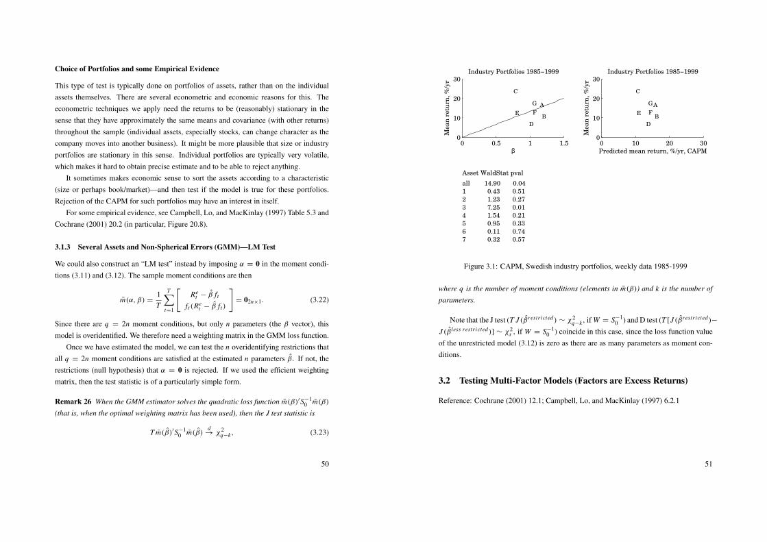
Choice of Portfolios and some Empirical Evidence

This type of test is typically done on portfolios of assets, rather than on the individualassets themselves. There are several econometric and economic reasons for this. Theeconometric techniques we apply need the returns to be (reasonably) stationary in thesense that they have approximately the same means and covariance (with other returns)throughout the sample (individual assets, especially stocks, can change character as thecompany moves into another business). It might be more plausible that size or industryportfolios are stationary in this sense. Individual portfolios are typically very volatile,which makes it hard to obtain precise estimate and to be able to reject anything.

It sometimes makes economic sense to sort the assets according to a characteristic(size or perhaps book/market)—and then test if the model is true for these portfolios.Rejection of the CAPM for such portfolios may have an interest in itself.

For some empirical evidence, see Campbell, Lo, and MacKinlay (1997) Table 5.3 andCochrane (2001) 20.2 (in particular, Figure 20.8).

3.1.3 Several Assets and Non-Spherical Errors (GMM)—LM Test

We could also construct an “LM test” instead by imposing α = 0 in the moment condi-tions (3.11) and (3.12). The sample moment conditions are then

m(α, β) =1T

T∑t=1

[Re

t − β ft

ft(Ret − β ft)

]= 02n×1. (3.22)

Since there are q = 2n moment conditions, but only n parameters (the β vector), thismodel is overidentified. We therefore need a weighting matrix in the GMM loss function.

Once we have estimated the model, we can test the n overidentifying restrictions thatall q = 2n moment conditions are satisfied at the estimated n parameters β. If not, therestrictions (null hypothesis) that α = 0 is rejected. If we used the efficient weightingmatrix, then the test statistic is of a particularly simple form.

Remark 26 When the GMM estimator solves the quadratic loss function m(β)′S−10 m(β)

(that is, when the optimal weighting matrix has been used), then the J test statistic is

T m(β)′S−10 m(β)

d→ χ2

q−k, (3.23)

50

0 0.5 1 1.50

10

20

30Industry Portfolios 1985−1999

β

Mea

n r

etu

rn,

%/y

r

A

B

C

D

E F

G

0 10 20 300

10

20

30Industry Portfolios 1985−1999

Predicted mean return, %/yr, CAPM

Mea

n r

etu

rn,

%/y

r

A

B

C

D

E F

G

Asset WaldStat pval

all 14.90 0.04

1 0.43 0.51

2 1.23 0.27

3 7.25 0.01

4 1.54 0.21

5 0.95 0.33

6 0.11 0.74

7 0.32 0.57

Figure 3.1: CAPM, Swedish industry portfolios, weekly data 1985-1999

where q is the number of moment conditions (elements in m(β)) and k is the number of

parameters.

Note that the J test (T J (βrestricted) ∼ χ2q−k, if W = S−1

0 ) and D test (T [J (βrestricted)−

J (βless restricted)] ∼ χ2s , if W = S−1

0 ) coincide in this case, since the loss function valueof the unrestricted model (3.12) is zero as there are as many parameters as moment con-ditions.

3.2 Testing Multi-Factor Models (Factors are Excess Returns)

Reference: Cochrane (2001) 12.1; Campbell, Lo, and MacKinlay (1997) 6.2.1

51

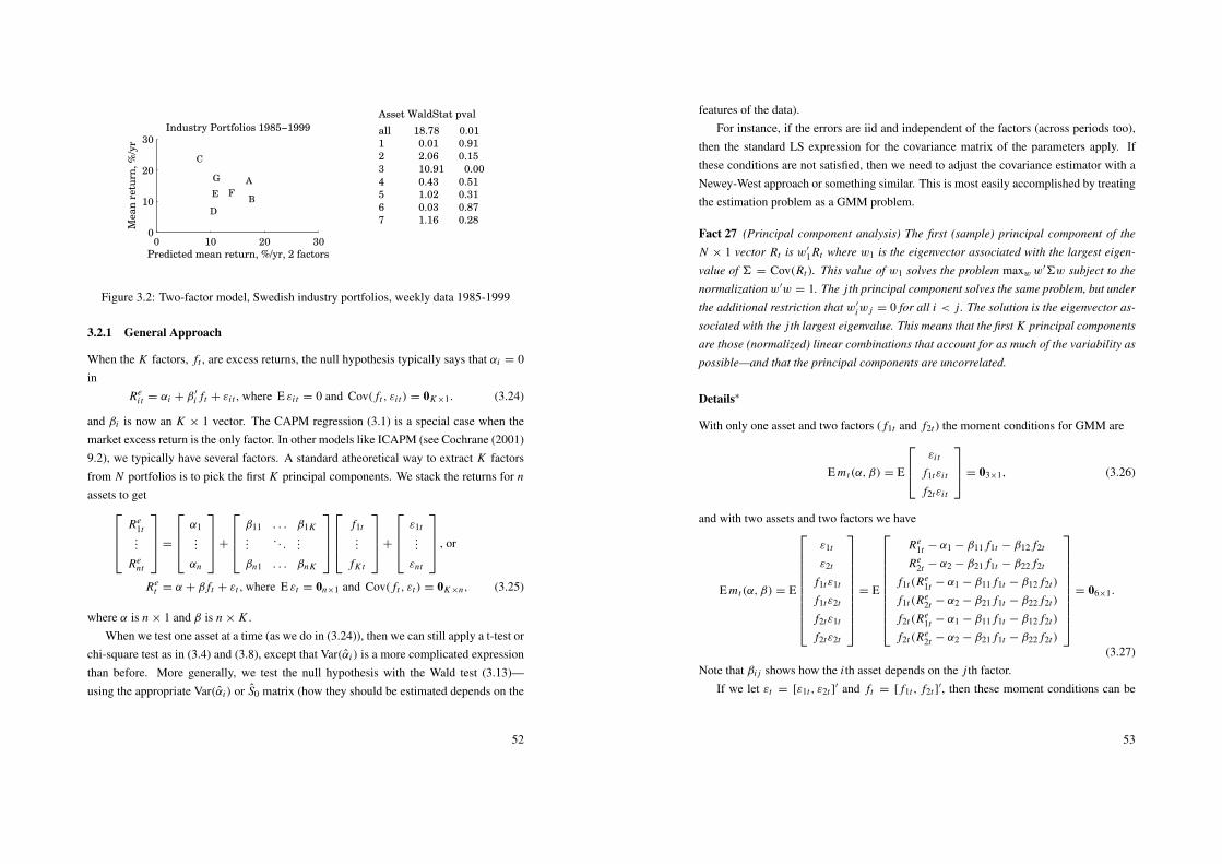
0 10 20 300

10

20

30Industry Portfolios 1985−1999

Predicted mean return, %/yr, 2 factors

Mea

n r

etu

rn,

%/y

r

A

B

C

D

E F

G

Asset WaldStat pval

all 18.78 0.01

1 0.01 0.91

2 2.06 0.15

3 10.91 0.00

4 0.43 0.51

5 1.02 0.31

6 0.03 0.87

7 1.16 0.28

Figure 3.2: Two-factor model, Swedish industry portfolios, weekly data 1985-1999

3.2.1 General Approach

When the K factors, ft , are excess returns, the null hypothesis typically says that αi = 0in

Rei t = αi + β ′

i ft + εi t , where E εi t = 0 and Cov( ft , εi t) = 0K×1. (3.24)

and βi is now an K × 1 vector. The CAPM regression (3.1) is a special case when themarket excess return is the only factor. In other models like ICAPM (see Cochrane (2001)9.2), we typically have several factors. A standard atheoretical way to extract K factorsfrom N portfolios is to pick the first K principal components. We stack the returns for n

assets to getRe

1t...

Rent

=

α1...

αn

+

β11 . . . β1K...

. . ....

βn1 . . . βnK

f1t...

fK t

+

ε1t...

εnt

, or

Ret = α + β ft + εt ,where E εt = 0n×1 and Cov( ft , εt) = 0K×n, (3.25)

where α is n × 1 and β is n × K .When we test one asset at a time (as we do in (3.24)), then we can still apply a t-test or

chi-square test as in (3.4) and (3.8), except that Var(αi ) is a more complicated expressionthan before. More generally, we test the null hypothesis with the Wald test (3.13)—using the appropriate Var(αi ) or S0 matrix (how they should be estimated depends on the

52

features of the data).For instance, if the errors are iid and independent of the factors (across periods too),

then the standard LS expression for the covariance matrix of the parameters apply. Ifthese conditions are not satisfied, then we need to adjust the covariance estimator with aNewey-West approach or something similar. This is most easily accomplished by treatingthe estimation problem as a GMM problem.

Fact 27 (Principal component analysis) The first (sample) principal component of the

N × 1 vector Rt is w′

1 Rt where w1 is the eigenvector associated with the largest eigen-

value of 6 = Cov(Rt). This value of w1 solves the problem maxw w′6w subject to the

normalizationw′w = 1. The j th principal component solves the same problem, but under

the additional restriction that w′

iw j = 0 for all i < j . The solution is the eigenvector as-

sociated with the j th largest eigenvalue. This means that the first K principal components

are those (normalized) linear combinations that account for as much of the variability as

possible—and that the principal components are uncorrelated.

Details∗

With only one asset and two factors ( f1t and f2t ) the moment conditions for GMM are

E mt(α, β) = E

εi t

f1tεi t

f2tεi t

= 03×1, (3.26)

and with two assets and two factors we have

E mt(α, β) = E

ε1t

ε2t

f1tε1t

f1tε2t

f2tε1t

f2tε2t

= E

Re1t − α1 − β11 f1t − β12 f2t

Re2t − α2 − β21 f1t − β22 f2t

f1t(Re1t − α1 − β11 f1t − β12 f2t)

f1t(Re2t − α2 − β21 f1t − β22 f2t)

f2t(Re1t − α1 − β11 f1t − β12 f2t)

f2t(Re2t − α2 − β21 f1t − β22 f2t)

= 06×1.

(3.27)Note that βi j shows how the i th asset depends on the j th factor.

If we let εt = [ε1t , ε2t ]′ and ft = [ f1t , f2t ]

′, then these moment conditions can be

53

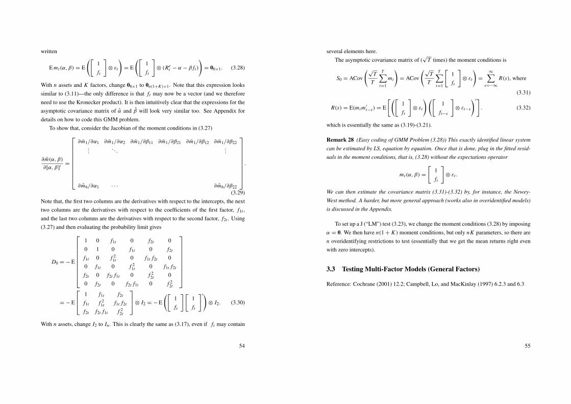
written

E mt(α, β) = E

([1ft

]⊗ εt

)= E

([1ft

]⊗ (Re

t − α − β ft)

)= 06×1. (3.28)

With n assets and K factors, change 06×1 to 0n(1+K )×1. Note that this expression lookssimilar to (3.11)—the only difference is that ft may now be a vector (and we thereforeneed to use the Kronecker product). It is then intuitively clear that the expressions for theasymptotic covariance matrix of α and β will look very similar too. See Appendix fordetails on how to code this GMM problem.

To show that, consider the Jacobian of the moment conditions in (3.27)

∂m(α, β)∂[α, β]′

=

∂m1/∂α1 ∂m1/∂α2 ∂m1/∂β11 ∂m1/∂β21 ∂m1/∂β12 ∂m1/∂β22...

. . ....

∂m6/∂α1 · · · ∂m6/∂β22

.

(3.29)Note that, the first two columns are the derivatives with respect to the intercepts, the nexttwo columns are the derivatives with respect to the coefficients of the first factor, f1t ,and the last two columns are the derivatives with respect to the second factor, f2t . Using(3.27) and then evaluating the probability limit gives

D0 = − E

1 0 f1t 0 f2t 00 1 0 f1t 0 f2t

f1t 0 f 21t 0 f1t f2t 0

0 f1t 0 f 21t 0 f1t f2t

f2t 0 f2t f1t 0 f 22t 0

0 f2t 0 f2t f1t 0 f 22t

= − E

1 f1t f2t

f1t f 21t f1t f2t

f2t f2t f1t f 22t

⊗ I2 = − E

([1ft

][1ft

]′)⊗ I2. (3.30)

With n assets, change I2 to In . This is clearly the same as (3.17), even if ft may contain

54

several elements here.The asymptotic covariance matrix of (

√T times) the moment conditions is

S0 = ACov

(√T

T

T∑t=1

mt

)= ACov

(√T

T

T∑t=1

[1ft

]⊗ εt

)=

∞∑s=−∞

R(s), where

(3.31)

R(s) = E(mtm′

t−s) = E

[([1ft

]⊗ εt

)([1

ft−s

]⊗ εt−s

)′]. (3.32)

which is essentially the same as (3.19)-(3.21).

Remark 28 (Easy coding of GMM Problem (3.28)) This exactly identified linear system

can be estimated by LS, equation by equation. Once that is done, plug in the fitted resid-

uals in the moment conditions, that is, (3.28) without the expectations operator

mt(α, β) =

[1ft

]⊗ εt .

We can then estimate the covariance matrix (3.31)-(3.32) by, for instance, the Newey-

West method. A harder, but more general approach (works also in overidentified models)

is discussed in the Appendix.

To set up a J (“LM”) test (3.23), we change the moment conditions (3.28) by imposingα = 0. We then have n(1 + K ) moment conditions, but only nK parameters, so there aren overidentifying restrictions to test (essentially that we get the mean returns right evenwith zero intercepts).

3.3 Testing Multi-Factor Models (General Factors)

Reference: Cochrane (2001) 12.2; Campbell, Lo, and MacKinlay (1997) 6.2.3 and 6.3

55

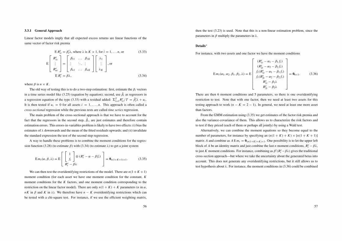
3.3.1 General Approach

Linear factor models imply that all expected excess returns are linear functions of thesame vector of factor risk premia

E Rei t = β ′

iλ, where λ is K × 1, for i = 1, . . . n, or (3.33)

E

Re

1t...

Rent

=

β11 . . . β1K...

. . ....

βn1 . . . βnK

λ1...

λK

, or

E Ret = βλ, (3.34)

where β is n × K .The old way of testing this is to do a two-step estimation: first, estimate the βi vectors

in a time series model like (3.25) (equation by equation); second, use βi as regressors ina regression equation of the type (3.33) with a residual added: 6T

t=1 Rei t/T = β ′

iλ + ui .It is then tested if ui = 0 for all assets i = 1, . . . , n. This approach is often called across-sectional regression while the previous tests are called time series regression.

The main problem of the cross-sectional approach is that we have to account for thefact that the regressors in the second step, βi , are just estimates and therefore containestimation errors. This errors-in-variables problem is likely to have two effects: (i) bias theestimates of λ downwards and the mean of the fitted residuals upwards; and (ii) invalidatethe standard expression the test of the second step regression.

A way to handle these problems is to combine the moment conditions for the regres-sion function (3.28) (to estimate β) with (3.34) (to estimate λ) to get a joint system

E mt(α, β, λ) = E

[

1ft

]⊗ (Re

t − α − β ft)

Ret − βλ

= 0n(1+K+1)×1. (3.35)

We can then test the overidentifying restrictions of the model. There are n(1 + K + 1)moment condition (for each asset we have one moment condition for the constant, K

moment conditions for the K factors, and one moment condition corresponding to therestriction on the linear factor model). There are only n(1 + K )+ K parameters (n in α,nK in β and K in λ). We therefore have n − K overidentifying restrictions which canbe tested with a chi-square test. For instance, if we use the efficient weighting matrix,

56

then the test (3.23) is used. Note that this is a non-linear estimation problem, since theparameters in β multiply the parameters in λ.

Details∗

For instance, with two assets and one factor we have the moment conditions

E mt(α1, α2, β1, β2, λ) = E

(Re1t − α1 − β1 ft)

(Re2t − α2 − β2 ft)

ft(Re1t − α1 − β1 ft)

ft(Re2t − α2 − β2 ft)

Re1t − β1λ

Re2t − β2λ

= 06×1. (3.36)

There are then 6 moment conditions and 5 parameters, so there is one overidentifyingrestriction to test. Note that with one factor, then we need at least two assets for thistesting approach to work (n − K = 2 − 1). In general, we need at least one more assetthan factors.

From the GMM estimation using (3.35) we get estimates of the factor risk premia andalso the variance-covariance of them. This allows us to characterize the risk factors andto test if they priced (each of them or perhaps all jointly) by using a Wald test.

Alternatively, we can combine the moment equations so they become equal to thenumber of parameters, for instance by specifying an (n(1 + K ) + K )× [n(1 + K + 1)]matrix A and combine as A E mt = 0(n(1+K )+K )×1. One possibility is to let the upper leftblock of A be an identity matrix and just combine the last n moment conditions, Re

t −βλ,to just K moment conditions. For instance, combining as β ′(Re

t −βλ) gives the traditionalcross-section approach—but where we take the uncertainty about the generated betas intoaccount. This does not generate any overidentifying restrictions, but it still allows us totest hypothesis about λ. For instance, the moment conditions in (3.36) could be combined

57

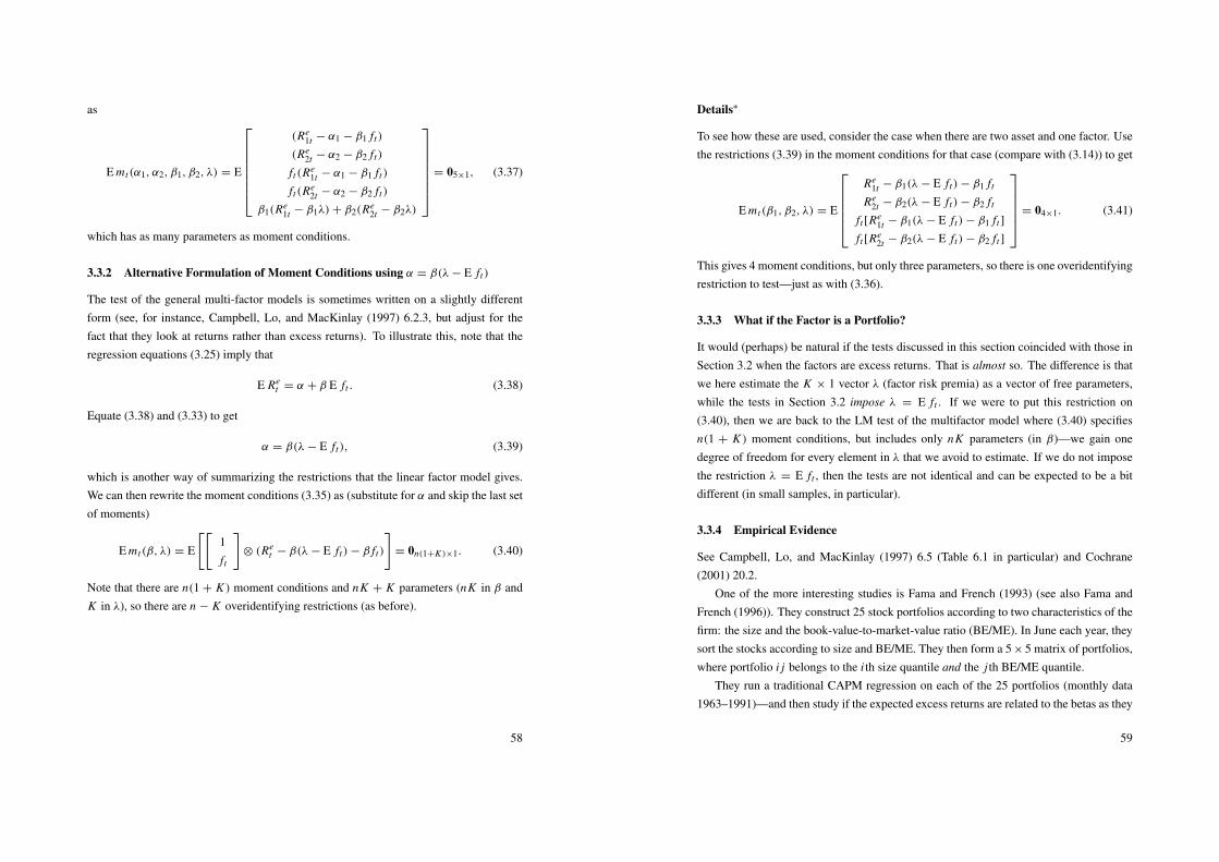
as

E mt(α1, α2, β1, β2, λ) = E

(Re

1t − α1 − β1 ft)

(Re2t − α2 − β2 ft)

ft(Re1t − α1 − β1 ft)

ft(Re2t − α2 − β2 ft)

β1(Re1t − β1λ)+ β2(Re

2t − β2λ)

= 05×1, (3.37)

which has as many parameters as moment conditions.

3.3.2 Alternative Formulation of Moment Conditions using α = β(λ− E ft)

The test of the general multi-factor models is sometimes written on a slightly differentform (see, for instance, Campbell, Lo, and MacKinlay (1997) 6.2.3, but adjust for thefact that they look at returns rather than excess returns). To illustrate this, note that theregression equations (3.25) imply that

E Ret = α + β E ft . (3.38)

Equate (3.38) and (3.33) to get

α = β(λ− E ft), (3.39)

which is another way of summarizing the restrictions that the linear factor model gives.We can then rewrite the moment conditions (3.35) as (substitute for α and skip the last setof moments)

E mt(β, λ) = E

[[1ft

]⊗ (Re

t − β(λ− E ft)− β ft)

]= 0n(1+K )×1. (3.40)

Note that there are n(1 + K ) moment conditions and nK + K parameters (nK in β andK in λ), so there are n − K overidentifying restrictions (as before).

58

Details∗

To see how these are used, consider the case when there are two asset and one factor. Usethe restrictions (3.39) in the moment conditions for that case (compare with (3.14)) to get

E mt(β1, β2, λ) = E

Re

1t − β1(λ− E ft)− β1 ft

Re2t − β2(λ− E ft)− β2 ft

ft [Re1t − β1(λ− E ft)− β1 ft ]

ft [Re2t − β2(λ− E ft)− β2 ft ]

= 04×1. (3.41)

This gives 4 moment conditions, but only three parameters, so there is one overidentifyingrestriction to test—just as with (3.36).

3.3.3 What if the Factor is a Portfolio?

It would (perhaps) be natural if the tests discussed in this section coincided with those inSection 3.2 when the factors are excess returns. That is almost so. The difference is thatwe here estimate the K × 1 vector λ (factor risk premia) as a vector of free parameters,while the tests in Section 3.2 impose λ = E ft . If we were to put this restriction on(3.40), then we are back to the LM test of the multifactor model where (3.40) specifiesn(1 + K ) moment conditions, but includes only nK parameters (in β)—we gain onedegree of freedom for every element in λ that we avoid to estimate. If we do not imposethe restriction λ = E ft , then the tests are not identical and can be expected to be a bitdifferent (in small samples, in particular).

3.3.4 Empirical Evidence

See Campbell, Lo, and MacKinlay (1997) 6.5 (Table 6.1 in particular) and Cochrane(2001) 20.2.

One of the more interesting studies is Fama and French (1993) (see also Fama andFrench (1996)). They construct 25 stock portfolios according to two characteristics of thefirm: the size and the book-value-to-market-value ratio (BE/ME). In June each year, theysort the stocks according to size and BE/ME. They then form a 5 × 5 matrix of portfolios,where portfolio i j belongs to the i th size quantile and the j th BE/ME quantile.

They run a traditional CAPM regression on each of the 25 portfolios (monthly data1963–1991)—and then study if the expected excess returns are related to the betas as they

59

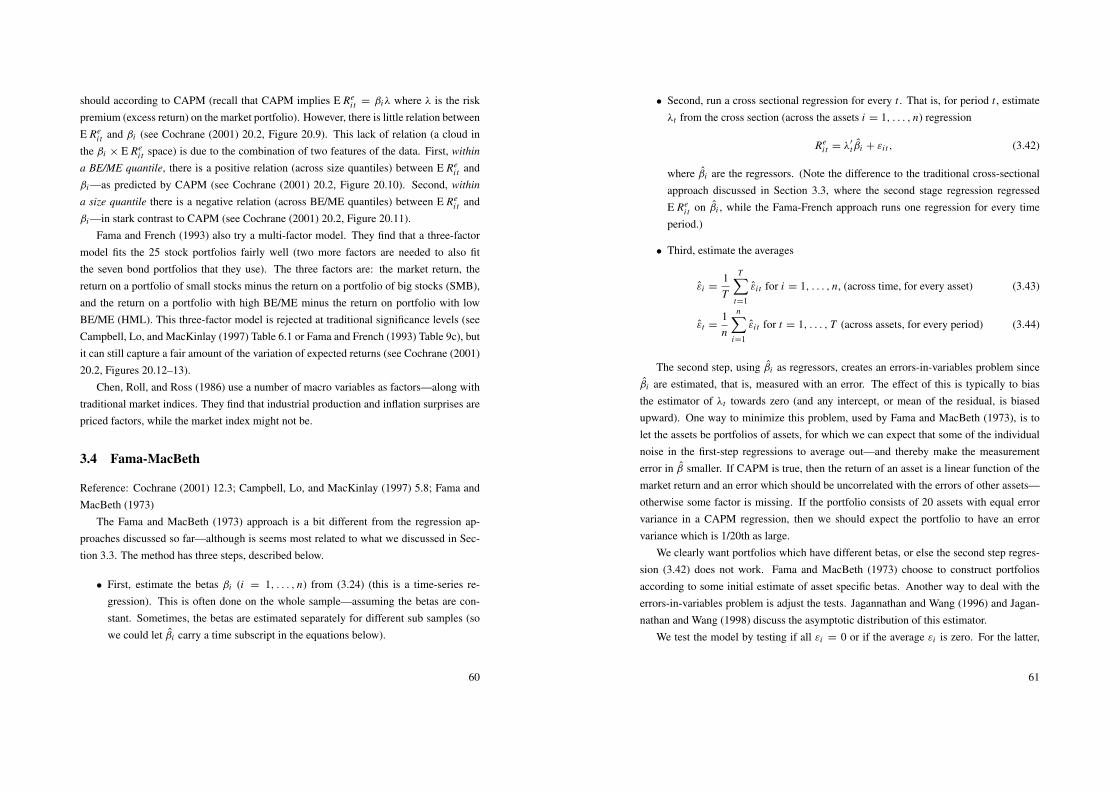
should according to CAPM (recall that CAPM implies E Rei t = βiλ where λ is the risk

premium (excess return) on the market portfolio). However, there is little relation betweenE Re

i t and βi (see Cochrane (2001) 20.2, Figure 20.9). This lack of relation (a cloud inthe βi × E Re

i t space) is due to the combination of two features of the data. First, within

a BE/ME quantile, there is a positive relation (across size quantiles) between E Rei t and

βi —as predicted by CAPM (see Cochrane (2001) 20.2, Figure 20.10). Second, within

a size quantile there is a negative relation (across BE/ME quantiles) between E Rei t and

βi —in stark contrast to CAPM (see Cochrane (2001) 20.2, Figure 20.11).Fama and French (1993) also try a multi-factor model. They find that a three-factor

model fits the 25 stock portfolios fairly well (two more factors are needed to also fitthe seven bond portfolios that they use). The three factors are: the market return, thereturn on a portfolio of small stocks minus the return on a portfolio of big stocks (SMB),and the return on a portfolio with high BE/ME minus the return on portfolio with lowBE/ME (HML). This three-factor model is rejected at traditional significance levels (seeCampbell, Lo, and MacKinlay (1997) Table 6.1 or Fama and French (1993) Table 9c), butit can still capture a fair amount of the variation of expected returns (see Cochrane (2001)20.2, Figures 20.12–13).

Chen, Roll, and Ross (1986) use a number of macro variables as factors—along withtraditional market indices. They find that industrial production and inflation surprises arepriced factors, while the market index might not be.

3.4 Fama-MacBeth

Reference: Cochrane (2001) 12.3; Campbell, Lo, and MacKinlay (1997) 5.8; Fama andMacBeth (1973)

The Fama and MacBeth (1973) approach is a bit different from the regression ap-proaches discussed so far—although is seems most related to what we discussed in Sec-tion 3.3. The method has three steps, described below.

• First, estimate the betas βi (i = 1, . . . , n) from (3.24) (this is a time-series re-gression). This is often done on the whole sample—assuming the betas are con-stant. Sometimes, the betas are estimated separately for different sub samples (sowe could let βi carry a time subscript in the equations below).

60

• Second, run a cross sectional regression for every t . That is, for period t , estimateλt from the cross section (across the assets i = 1, . . . , n) regression

Rei t = λ′

t βi + εi t , (3.42)

where βi are the regressors. (Note the difference to the traditional cross-sectionalapproach discussed in Section 3.3, where the second stage regression regressedE Re

i t on βi , while the Fama-French approach runs one regression for every timeperiod.)

• Third, estimate the averages

εi =1T

T∑t=1

εi t for i = 1, . . . , n, (across time, for every asset) (3.43)

εt =1n

n∑i=1

εi t for t = 1, . . . , T (across assets, for every period) (3.44)

The second step, using βi as regressors, creates an errors-in-variables problem sinceβi are estimated, that is, measured with an error. The effect of this is typically to biasthe estimator of λt towards zero (and any intercept, or mean of the residual, is biasedupward). One way to minimize this problem, used by Fama and MacBeth (1973), is tolet the assets be portfolios of assets, for which we can expect that some of the individualnoise in the first-step regressions to average out—and thereby make the measurementerror in β smaller. If CAPM is true, then the return of an asset is a linear function of themarket return and an error which should be uncorrelated with the errors of other assets—otherwise some factor is missing. If the portfolio consists of 20 assets with equal errorvariance in a CAPM regression, then we should expect the portfolio to have an errorvariance which is 1/20th as large.

We clearly want portfolios which have different betas, or else the second step regres-sion (3.42) does not work. Fama and MacBeth (1973) choose to construct portfoliosaccording to some initial estimate of asset specific betas. Another way to deal with theerrors-in-variables problem is adjust the tests. Jagannathan and Wang (1996) and Jagan-nathan and Wang (1998) discuss the asymptotic distribution of this estimator.

We test the model by testing if all εi = 0 or if the average εi is zero. For the latter,

61

Fama and MacBeth (1973) suggest that the test should use the following estimator of thevariance

Var

(√T

T

T∑t=1

εt

)=

1T

T∑t=1

(εt − εt

)2, (3.45)

where εt is the sample average of εt , εt = 6Tt=1εt/T . Note that this is the standard

formula for the variance of√

T times a sample average for an iid variable (which equalsthe variance of the series itself). It is, of course, unclear if that assumption is valid.

If, instead, we want to test if εi = 0 for all assets (i = 1, . . . , n), we need the wholecovariance matrix for the vector of εi . They are estimated under the same iid assumptionas above

Cov

√

TT

T∑t=1

ε1...

εn

=

1T

T∑t=1

ε1t...

εnt

−

ε1t...

εnt

ε1t...

εnt

−

ε1t...

εnt

′

,

(3.46)where εi t = 6T

t=1εi t/T . Once we have this covariance matrix, we can test the hypothesisthat εi = 0 for all assets (i = 1, . . . , n) by the usual chi-square test.

Fama and MacBeth (1973) found, among other things, that the squared beta is notsignificant in the second step regression, nor is a measure of non-systematic risk.

A Coding of the GMM Problem in Section 3.2

This section describes how the GMM problem with the moment conditions (3.28) can beprogrammed.

A.1 Exactly Identified System

The moments are

mt(α, β) =

[1ft

]⊗

(Re

t −

[α β

] [ 1ft

]).

We want to rewrite this on a form where the parameters are collected in a vector, so thatwe easily can apply matrix algebra to find the parameter estimates. To do that, notice the

62

following rules for Kronecker products: (i) vec(ABC) = (C ′⊗ A)vec(B); (ii) (A⊗ B)′ =

A′⊗ B ′; and (iii) if a is m × 1 and b is n × 1, then a ⊗ b = (a ⊗ In)b. The first rule

allows to write

In

[α β

] [ 1ft

]=

([1ft

]′

⊗ In

)︸ ︷︷ ︸

x ′t

vec([α β

])︸ ︷︷ ︸

b

.

The third rule allows us two rewrite the moments as

mt(α, β) =

([1ft

]⊗ In

)︸ ︷︷ ︸

xt

(Re

t −

[α β

] [ 1ft

]),

where the second rule helped us identify the leading term as the transpose of x ′t in the

previous equation. We therefore have

mt(α, β) =

([1ft

]⊗ In

)︸ ︷︷ ︸

xt

Ret −

([1ft

]′

⊗ In

)︸ ︷︷ ︸

x ′t

b

.

To compare with the LS case, let yt = Ret . We can then write the moment conditions as

mt(α, β) = xt(yt − x ′

tb)

= xt yt − xt x ′

tb.

In the exactly identified case, we can solve for the b vector from 6Tt=1mt/T = 0. To do

that, define

6xy =1T

T∑t=1

xt yt and 6xx =1T

T∑t=1

xt x ′

t , so

6Tt=1mt/T = 6xy −6xxb = 0 or b = 6−1

xx 6xy.

This looks very similar to the standard LS, but there is a hitch: xt is an n(1 + K )× n

matrix, not a vector. It is still possible to compute the vector6xy (dimension (1+K )n×1)and the matrix 6xx (dimension (1 + K )n × (1 + K )n) efficiently, since they have very

63

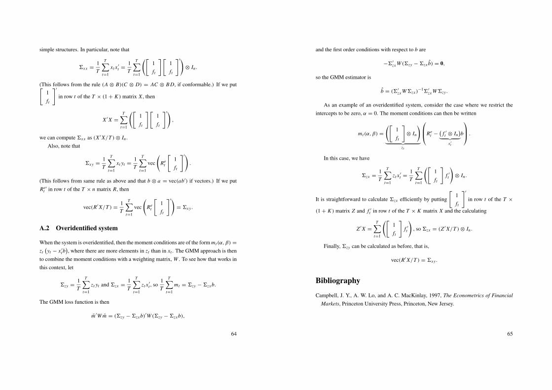
simple structures. In particular, note that

6xx =1T

T∑t=1

xt x ′

t =1T

T∑t=1

([1ft

][1ft

]′)⊗ In.

(This follows from the rule (A ⊗ B)(C ⊗ D) = AC ⊗ B D, if conformable.) If we put[1ft

]′

in row t of the T × (1 + K ) matrix X , then

X ′X =

T∑t=1

([1ft

][1ft

]′),

we can compute 6xx as (X ′X/T )⊗ In .Also, note that

6xy =1T

T∑t=1

xt yt =1T

T∑t=1

vec

(Re

t

[1ft

]′).

(This follows from same rule as above and that b ⊗ a = vec(ab′) if vectors.) If we putRe′

t in row t of the T × n matrix R, then

vec(R′X/T ) =1T

T∑t=1

vec

(Re

t

[1ft

]′)= 6xy.

A.2 Overidentified system

When the system is overidentified, then the moment conditions are of the form mt(α, β) =

zt(yt − x ′

tb), where there are more elements in zt than in xt . The GMM approach is then

to combine the moment conditions with a weighting matrix, W . To see how that works inthis context, let

6zy =1T

T∑t=1

zt yt and 6zx =1T

T∑t=1

zt x ′

t , so1T

T∑t=1

mt = 6zy −6zxb.

The GMM loss function is then

m′W m = (6zy −6zxb)′W (6zy −6zxb),

64

and the first order conditions with respect to b are

−6′

zx W (6zy −6zx b) = 0,

so the GMM estimator is

b = (6′

zx W6zx)−16′

zx W6zy.

As an example of an overidentified system, consider the case where we restrict theintercepts to be zero, α = 0. The moment conditions can then be written

mt(α, β) =

([1ft

]⊗ In

)︸ ︷︷ ︸

zt

Ret −

(f ′

t ⊗ In)︸ ︷︷ ︸

x ′t

b

.In this case, we have

6zx =1T

T∑t=1

zt x ′

t =1T

T∑t=1

([1ft

]f ′

t

)⊗ In.

It is straightforward to calculate 6zx efficiently by putting

[1ft

]′

in row t of the T ×

(1 + K ) matrix Z and f ′t in row t of the T × K matrix X and the calculating

Z ′X =

T∑t=1

([1ft

]f ′

t

), so 6zx = (Z ′X/T )⊗ In.

Finally, 6zy can be calculated as before, that is,

vec(R′X/T ) = 6xy.

Bibliography

Campbell, J. Y., A. W. Lo, and A. C. MacKinlay, 1997, The Econometrics of Financial

Markets, Princeton University Press, Princeton, New Jersey.

65

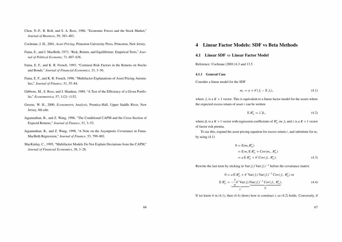
Chen, N.-F., R. Roll, and S. A. Ross, 1986, “Economic Forces and the Stock Market,”Journal of Business, 59, 383–403.

Cochrane, J. H., 2001, Asset Pricing, Princeton University Press, Princeton, New Jersey.

Fama, E., and J. MacBeth, 1973, “Risk, Return, and Equilibrium: Empirical Tests,” Jour-

nal of Political Economy, 71, 607–636.

Fama, E. F., and K. R. French, 1993, “Common Risk Factors in the Returns on Stocksand Bonds,” Journal of Financial Economics, 33, 3–56.

Fama, E. F., and K. R. French, 1996, “Multifactor Explanations of Asset Pricing Anoma-lies,” Journal of Finance, 51, 55–84.

Gibbons, M., S. Ross, and J. Shanken, 1989, “A Test of the Efficiency of a Given Portfo-lio,” Econometrica, 57, 1121–1152.

Greene, W. H., 2000, Econometric Analysis, Prentice-Hall, Upper Saddle River, NewJersey, 4th edn.

Jagannathan, R., and Z. Wang, 1996, “The Conditional CAPM and the Cross-Section ofExpectd Returns,” Journal of Finance, 51, 3–53.

Jagannathan, R., and Z. Wang, 1998, “A Note on the Asymptotic Covariance in Fama-MacBeth Regression,” Journal of Finance, 53, 799–801.

MacKinlay, C., 1995, “Multifactor Models Do Not Explain Deviations from the CAPM,”Journal of Financial Economics, 38, 3–28.

66

4 Linear Factor Models: SDF vs Beta Methods

4.1 Linear SDF ⇔ Linear Factor Model

Reference: Cochrane (2001) 6.3 and 13.5

4.1.1 General Case

Consider a linear model for the SDF

mt = a + b′( ft − E ft), (4.1)

where ft is a K × 1 vector. This is equivalent to a linear factor model for the assets wherethe expected excess return of asset i can be written

E Rei t = λ′βi , (4.2)

where βi is a K ×1 vector with regression coefficients of Rei t on ft and λ is a K ×1 vector

of factor risk premia.To see this, expand the asset pricing equation for excess return i , and substitute for mt

by using (4.1)

0 = E(mt Rei t)

= E mt E Rei t + Cov(mt , Re

i t)

= a E Rei t + b′ Cov( ft , Re

i t). (4.3)

Rewrite the last term by sticking in Var( ft)Var( ft)−1 before the covariance matrix

0 = a E Rei t + b′ Var( ft)Var( ft)

−1 Cov( ft , Rei t) or

E Rei t = −

1a

b′ Var( ft)︸ ︷︷ ︸λ′

Var( ft)−1 Cov( ft , Re

i t)︸ ︷︷ ︸βi

. (4.4)

If we know b in (4.1), then (4.4) shows how to construct λ so (4.2) holds. Conversely, if

67

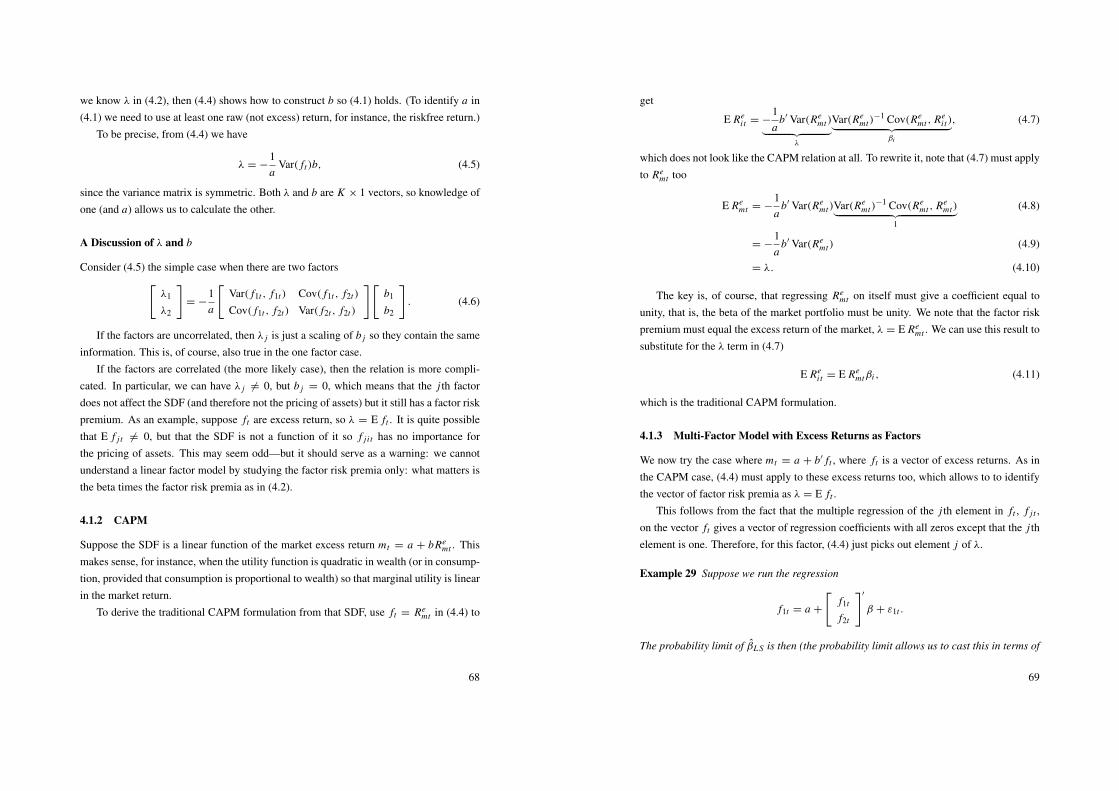
we know λ in (4.2), then (4.4) shows how to construct b so (4.1) holds. (To identify a in(4.1) we need to use at least one raw (not excess) return, for instance, the riskfree return.)

To be precise, from (4.4) we have

λ = −1a

Var( ft)b, (4.5)

since the variance matrix is symmetric. Both λ and b are K × 1 vectors, so knowledge ofone (and a) allows us to calculate the other.

A Discussion of λ and b

Consider (4.5) the simple case when there are two factors[λ1

λ2

]= −

1a

[Var( f1t , f1t) Cov( f1t , f2t)

Cov( f1t , f2t) Var( f2t , f2t)

][b1

b2

]. (4.6)

If the factors are uncorrelated, then λ j is just a scaling of b j so they contain the sameinformation. This is, of course, also true in the one factor case.

If the factors are correlated (the more likely case), then the relation is more compli-cated. In particular, we can have λ j 6= 0, but b j = 0, which means that the j th factordoes not affect the SDF (and therefore not the pricing of assets) but it still has a factor riskpremium. As an example, suppose ft are excess return, so λ = E ft . It is quite possiblethat E f j t 6= 0, but that the SDF is not a function of it so f j i t has no importance forthe pricing of assets. This may seem odd—but it should serve as a warning: we cannotunderstand a linear factor model by studying the factor risk premia only: what matters isthe beta times the factor risk premia as in (4.2).

4.1.2 CAPM

Suppose the SDF is a linear function of the market excess return mt = a + bRemt . This

makes sense, for instance, when the utility function is quadratic in wealth (or in consump-tion, provided that consumption is proportional to wealth) so that marginal utility is linearin the market return.

To derive the traditional CAPM formulation from that SDF, use ft = Remt in (4.4) to

68

get

E Rei t = −

1a

b′ Var(Remt)︸ ︷︷ ︸

λ

Var(Remt)

−1 Cov(Remt , Re

i t)︸ ︷︷ ︸βi

, (4.7)

which does not look like the CAPM relation at all. To rewrite it, note that (4.7) must applyto Re

mt too

E Remt = −

1a

b′ Var(Remt)Var(Re

mt)−1 Cov(Re

mt , Remt)︸ ︷︷ ︸

1

(4.8)

= −1a

b′ Var(Remt) (4.9)

= λ. (4.10)

The key is, of course, that regressing Remt on itself must give a coefficient equal to

unity, that is, the beta of the market portfolio must be unity. We note that the factor riskpremium must equal the excess return of the market, λ = E Re

mt . We can use this result tosubstitute for the λ term in (4.7)

E Rei t = E Re

mtβi , (4.11)

which is the traditional CAPM formulation.

4.1.3 Multi-Factor Model with Excess Returns as Factors

We now try the case where mt = a + b′ ft , where ft is a vector of excess returns. As inthe CAPM case, (4.4) must apply to these excess returns too, which allows to to identifythe vector of factor risk premia as λ = E ft .

This follows from the fact that the multiple regression of the j th element in ft , f j t ,on the vector ft gives a vector of regression coefficients with all zeros except that the j thelement is one. Therefore, for this factor, (4.4) just picks out element j of λ.

Example 29 Suppose we run the regression

f1t = a +

[f1t

f2t

]′

β + ε1t .

The probability limit of βL S is then (the probability limit allows us to cast this in terms of

69

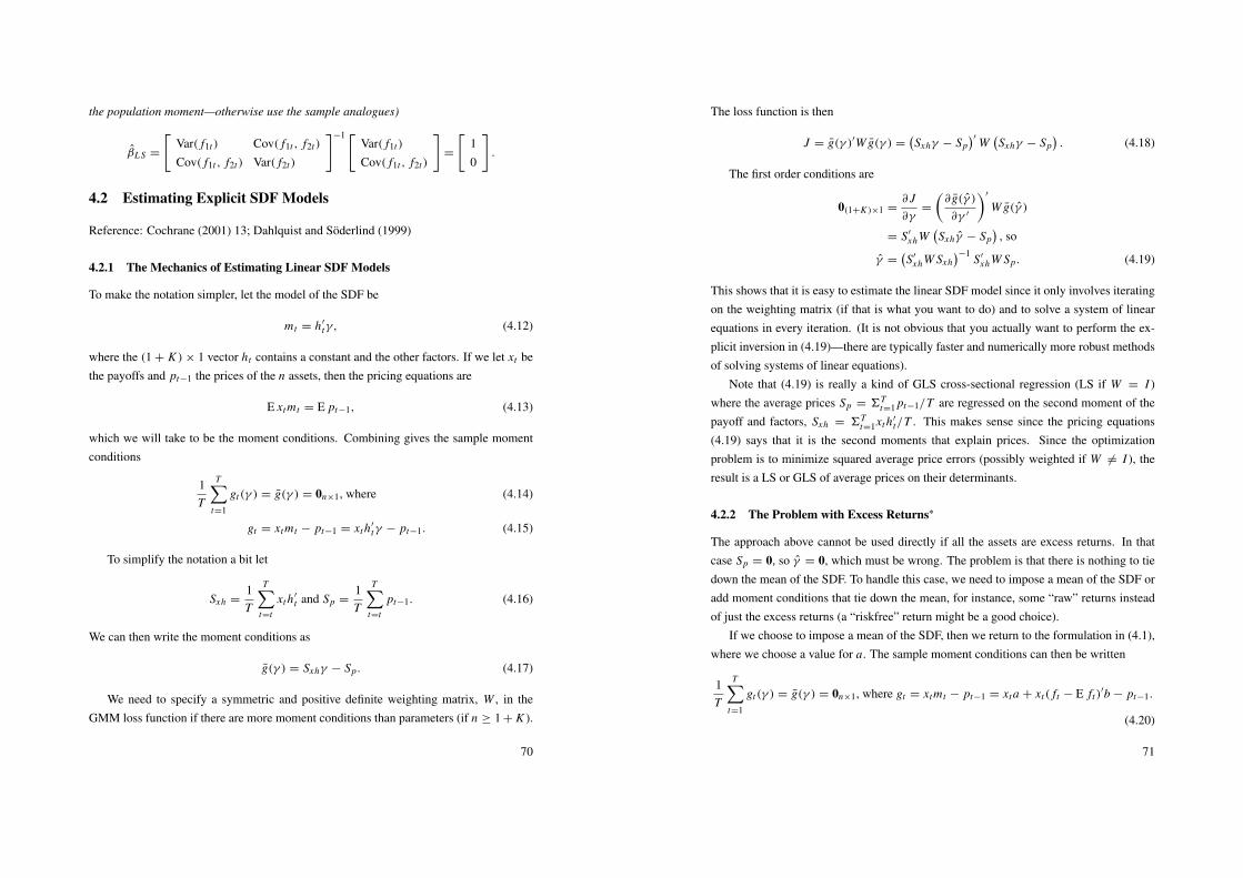
the population moment—otherwise use the sample analogues)

βL S =

[Var( f1t) Cov( f1t , f2t)

Cov( f1t , f2t) Var( f2t)

]−1 [Var( f1t)

Cov( f1t , f2t)

]=

[10

].

4.2 Estimating Explicit SDF Models

Reference: Cochrane (2001) 13; Dahlquist and Soderlind (1999)

4.2.1 The Mechanics of Estimating Linear SDF Models

To make the notation simpler, let the model of the SDF be

mt = h′

tγ, (4.12)

where the (1 + K )× 1 vector ht contains a constant and the other factors. If we let xt bethe payoffs and pt−1 the prices of the n assets, then the pricing equations are

E xtmt = E pt−1, (4.13)

which we will take to be the moment conditions. Combining gives the sample momentconditions

1T

T∑t=1

gt(γ ) = g(γ ) = 0n×1, where (4.14)

gt = xtmt − pt−1 = xt h′

tγ − pt−1. (4.15)

To simplify the notation a bit let

Sxh =1T

T∑t=t

xt h′

t and Sp =1T

T∑t=t

pt−1. (4.16)

We can then write the moment conditions as

g(γ ) = Sxhγ − Sp. (4.17)

We need to specify a symmetric and positive definite weighting matrix, W , in theGMM loss function if there are more moment conditions than parameters (if n ≥ 1 + K ).

70

The loss function is then

J = g(γ )′W g(γ ) =(Sxhγ − Sp

)′ W(Sxhγ − Sp

). (4.18)

The first order conditions are

0(1+K )×1 =∂ J∂γ

=

(∂ g(γ )∂γ ′

)′

W g(γ )

= S′

xhW(Sxh γ − Sp

), so

γ =(S′

xhW Sxh)−1 S′

xhW Sp. (4.19)

This shows that it is easy to estimate the linear SDF model since it only involves iteratingon the weighting matrix (if that is what you want to do) and to solve a system of linearequations in every iteration. (It is not obvious that you actually want to perform the ex-plicit inversion in (4.19)—there are typically faster and numerically more robust methodsof solving systems of linear equations).

Note that (4.19) is really a kind of GLS cross-sectional regression (LS if W = I )where the average prices Sp = 6T

t=1 pt−1/T are regressed on the second moment of thepayoff and factors, Sxh = 6T

t=1xt h′t/T . This makes sense since the pricing equations

(4.19) says that it is the second moments that explain prices. Since the optimizationproblem is to minimize squared average price errors (possibly weighted if W 6= I ), theresult is a LS or GLS of average prices on their determinants.

4.2.2 The Problem with Excess Returns∗

The approach above cannot be used directly if all the assets are excess returns. In thatcase Sp = 0, so γ = 0, which must be wrong. The problem is that there is nothing to tiedown the mean of the SDF. To handle this case, we need to impose a mean of the SDF oradd moment conditions that tie down the mean, for instance, some “raw” returns insteadof just the excess returns (a “riskfree” return might be a good choice).

If we choose to impose a mean of the SDF, then we return to the formulation in (4.1),where we choose a value for a. The sample moment conditions can then be written

1T

T∑t=1

gt(γ ) = g(γ ) = 0n×1, where gt = xtmt − pt−1 = xta + xt( ft − E ft)′b − pt−1.

(4.20)

71

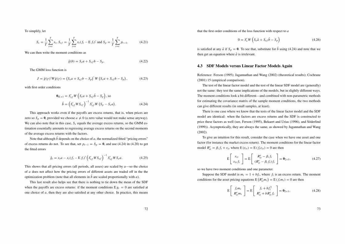
To simplify, let

Sx =1T

T∑t=t

xt , Sx f =1T

T∑t=t

xt( ft − E ft)′ and Sp =

1T

T∑t=t

pt−1. (4.21)

We can then write the moment conditions as

g(b) = Sxa + Sx f b − Sp. (4.22)

The GMM loss function is

J = g(γ )′W g(γ ) =(Sxa + Sx f b − Sp

)′ W(Sxa + Sx f b − Sp

), (4.23)

with first order conditions

0K×1 = S′

x f W(

Sxa + Sx f b − Sp

), so

b =

(S′

x f W Sx f

)−1S′

x f W(Sp − Sxa

). (4.24)

This approach works even if the payoffs are excess returns, that is, when prices arezero so Sp = 0, provided we choose a 6= 0 (a zero value would not make sense anyway).We can also note that in this case, Sx equals the average excess returns, so the GMM es-timation essentially amounts to regressing average excess returns on the second momentsof the average excess returns with the factors.

Note that although b depends on the choice of a, the normalized fitted “pricing errors”of excess returns do not. To see that, set pt−1 = Sp = 0, and use (4.24) in (4.20) to getthe fitted errors

gt = xta − xt( ft − E ft)′

(S′

x f W Sx f

)−1S′

x f W Sxa. (4.25)

This shows that all pricing errors (all periods, all asses) are scaled by a—so the choiceof a does not affect how the pricing errors of different assets are traded off in the theoptimization problem (note that all elements in b are scaled proportionally with a).

This last result also helps see that there is nothing to tie down the mean of the SDFwhen the payoffs are excess returns: if the moment conditions E gt = 0 are satisfied atone choice of a, then they are also satisfied at any other choice. In practice, this means

72

that the first order conditions of the loss function with respect to a

0 = S′

x W(

Sx a + Sx f b − Sp

)(4.26)

is satisfied at any a if Sp = 0. To see that, substitute for b using (4.24) and note that wethen get an equation where a is irrelevant.

4.3 SDF Models versus Linear Factor Models Again

Reference: Ferson (1995); Jagannathan and Wang (2002) (theoretical results); Cochrane(2001) 15 (empirical comparison).

The test of the linear factor model and the test of the linear SDF model are (generally)not the same: they test the same implications of the models, but in slightly different ways.The moment conditions look a bit different—and combined with non-parametric methodsfor estimating the covariance matrix of the sample moment conditions, the two methodscan give different results (in small samples, at least).

There is one case where we know that the tests of the linear factor model and the SDFmodel are identical: when the factors are excess returns and the SDF is constructed toprice these factors as well (see, Ferson (1995), Bekaert and Urias (1996), and Soderlind(1999)). Asymptotically, they are always the same, as showed by Jagannathan and Wang(2002).

To give an intuition for this result, consider the case when we have one asset and onefactor (for instance the market excess return). The moment conditions for the linear factormodel Re

i t = βi ft + εi t where E (εi t) = E ( ftεi t) = 0 are then

E

[εi t

εi t ft

]= E

[Re

i t − βi ft

(Rei t − βi ft) ft

]= 02×1, (4.27)

so we have two moment conditions and one parameter.Suppose the SDF model is mt = 1 + b ft , where ft is an excess return. The moment

conditions for the asset pricing equations E(Re

i tmt)

= E ( ftmt) = 0 are then

E

[ftmt

Rei tmt

]= E

[ft + b f 2

t

Rei t + bRe

i t ft

]= 02×1, (4.28)

73

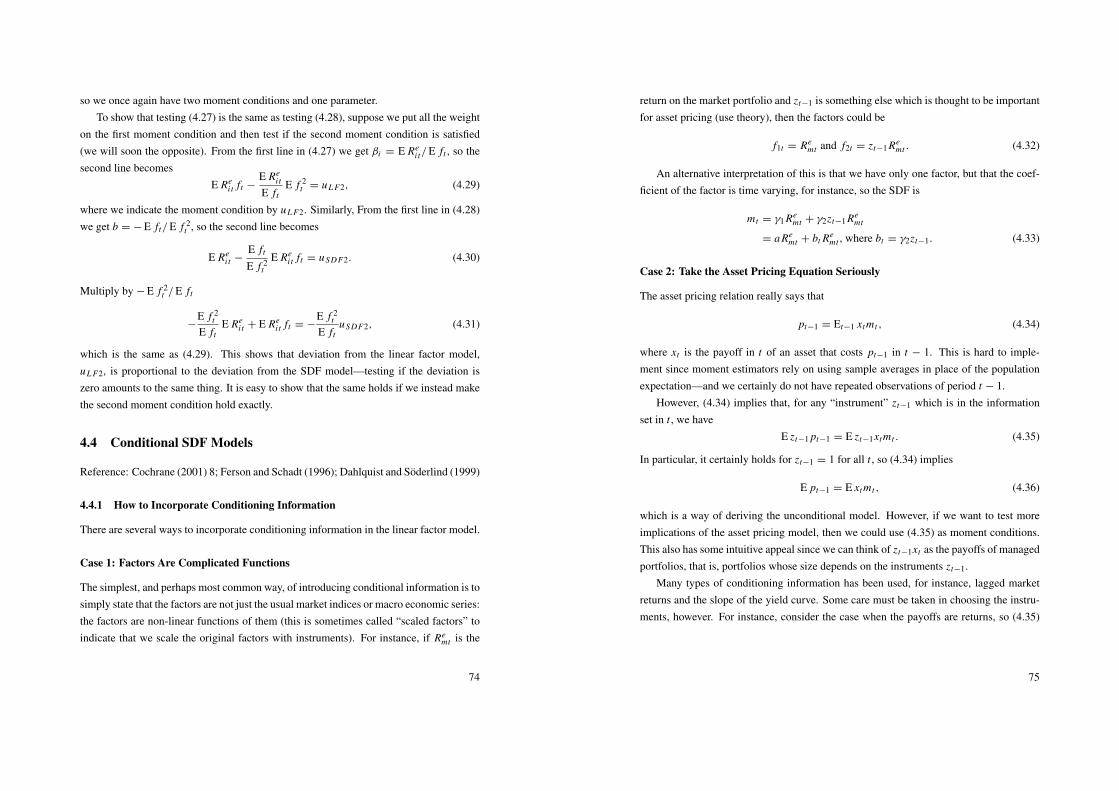
so we once again have two moment conditions and one parameter.To show that testing (4.27) is the same as testing (4.28), suppose we put all the weight

on the first moment condition and then test if the second moment condition is satisfied(we will soon the opposite). From the first line in (4.27) we get βi = E Re

i t/E ft , so thesecond line becomes

E Rei t ft −

E Rei t

E ftE f 2

t = uL F2, (4.29)

where we indicate the moment condition by uL F2. Similarly, From the first line in (4.28)we get b = − E ft/E f 2

t , so the second line becomes

E Rei t −

E ft

E f 2t

E Rei t ft = uSDF2. (4.30)

Multiply by − E f 2t /E ft

−E f 2

t

E ftE Re

i t + E Rei t ft = −

E f 2t

E ftuSDF2, (4.31)

which is the same as (4.29). This shows that deviation from the linear factor model,uL F2, is proportional to the deviation from the SDF model—testing if the deviation iszero amounts to the same thing. It is easy to show that the same holds if we instead makethe second moment condition hold exactly.

4.4 Conditional SDF Models

Reference: Cochrane (2001) 8; Ferson and Schadt (1996); Dahlquist and Soderlind (1999)

4.4.1 How to Incorporate Conditioning Information

There are several ways to incorporate conditioning information in the linear factor model.

Case 1: Factors Are Complicated Functions

The simplest, and perhaps most common way, of introducing conditional information is tosimply state that the factors are not just the usual market indices or macro economic series:the factors are non-linear functions of them (this is sometimes called “scaled factors” toindicate that we scale the original factors with instruments). For instance, if Re

mt is the

74

return on the market portfolio and zt−1 is something else which is thought to be importantfor asset pricing (use theory), then the factors could be

f1t = Remt and f2t = zt−1 Re

mt . (4.32)

An alternative interpretation of this is that we have only one factor, but that the coef-ficient of the factor is time varying, for instance, so the SDF is

mt = γ1 Remt + γ2zt−1 Re

mt

= a Remt + bt Re

mt , where bt = γ2zt−1. (4.33)

Case 2: Take the Asset Pricing Equation Seriously

The asset pricing relation really says that

pt−1 = Et−1 xtmt , (4.34)

where xt is the payoff in t of an asset that costs pt−1 in t − 1. This is hard to imple-ment since moment estimators rely on using sample averages in place of the populationexpectation—and we certainly do not have repeated observations of period t − 1.

However, (4.34) implies that, for any “instrument” zt−1 which is in the informationset in t , we have

E zt−1 pt−1 = E zt−1xtmt . (4.35)

In particular, it certainly holds for zt−1 = 1 for all t , so (4.34) implies

E pt−1 = E xtmt , (4.36)

which is a way of deriving the unconditional model. However, if we want to test moreimplications of the asset pricing model, then we could use (4.35) as moment conditions.This also has some intuitive appeal since we can think of zt−1xt as the payoffs of managedportfolios, that is, portfolios whose size depends on the instruments zt−1.

Many types of conditioning information has been used, for instance, lagged marketreturns and the slope of the yield curve. Some care must be taken in choosing the instru-ments, however. For instance, consider the case when the payoffs are returns, so (4.35)

75

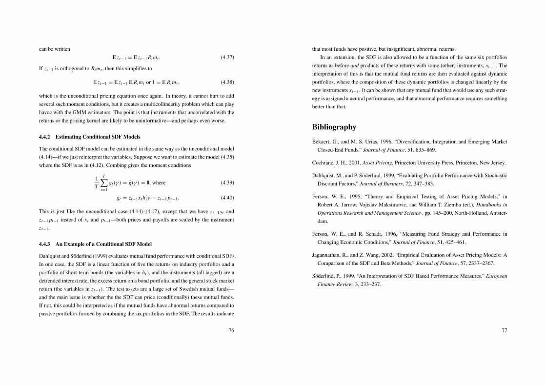
can be writtenE zt−1 = E zt−1 Rtmt . (4.37)

If zt−1 is orthogonal to Rtmt , then this simplifies to

E zt−1 = E zt−1 E Rtmt or 1 = E Rtmt , (4.38)

which is the unconditional pricing equation once again. In theory, it cannot hurt to addseveral such moment conditions, but it creates a multicollinearity problem which can playhavoc with the GMM estimators. The point is that instruments that uncorrelated with thereturns or the pricing kernel are likely to be uninformative—and perhaps even worse.

4.4.2 Estimating Conditional SDF Models

The conditional SDF model can be estimated in the same way as the unconditional model(4.14)—if we just reinterpret the variables. Suppose we want to estimate the model (4.35)where the SDF is as in (4.12). Combing gives the moment conditions

1T

T∑t=1

gt(γ ) = g(γ ) = 0, where (4.39)

gt = zt−1xt h′

tγ − zt−1 pt−1. (4.40)

This is just like the unconditional case (4.14)–(4.17), except that we have zt−1xt andzt−1 pt−1 instead of xt and pt−1—both prices and payoffs are scaled by the instrumentzt−1.

4.4.3 An Example of a Conditional SDF Model

Dahlquist and Soderlind (1999) evaluates mutual fund performance with conditional SDFs.In one case, the SDF is a linear function of five the returns on industry portfolios and aportfolio of short-term bonds (the variables in ht ), and the instruments (all lagged) are adetrended interest rate, the excess return on a bond portfolio, and the general stock marketreturn (the variables in zt−1). The test assets are a large set of Swedish mutual funds—and the main issue is whether the the SDF can price (conditionally) these mutual funds.If not, this could be interpreted as if the mutual funds have abnormal returns compared topassive portfolios formed by combining the six portfolios in the SDF. The results indicate

76

that most funds have positive, but insignificant, abnormal returns.In an extension, the SDF is also allowed to be a function of the same six portfolios

returns as before and products of these returns with some (other) instruments, xt−1. Theinterpretation of this is that the mutual fund returns are then evaluated against dynamicportfolios, where the composition of these dynamic portfolios is changed linearly by thenew instruments xt−1. It can be shown that any mutual fund that would use any such strat-egy is assigned a neutral performance, and that abnormal performance requires somethingbetter than that.

Bibliography

Bekaert, G., and M. S. Urias, 1996, “Diversification, Integration and Emerging MarketClosed-End Funds,” Journal of Finance, 51, 835–869.

Cochrane, J. H., 2001, Asset Pricing, Princeton University Press, Princeton, New Jersey.

Dahlquist, M., and P. Soderlind, 1999, “Evaluating Portfolio Performance with StochasticDiscount Factors,” Journal of Business, 72, 347–383.

Ferson, W. E., 1995, “Theory and Empirical Testing of Asset Pricing Models,” inRobert A. Jarrow, Vojislav Maksimovic, and William T. Ziemba (ed.), Handbooks in

Operations Research and Management Science . pp. 145–200, North-Holland, Amster-dam.

Ferson, W. E., and R. Schadt, 1996, “Measuring Fund Strategy and Performance inChanging Economic Conditions,” Journal of Finance, 51, 425–461.

Jagannathan, R., and Z. Wang, 2002, “Empirical Evaluation of Asset Pricing Models: AComparison of the SDF and Beta Methods,” Journal of Finance, 57, 2337–2367.

Soderlind, P., 1999, “An Interpretation of SDF Based Performance Measures,” European

Finance Review, 3, 233–237.

77

5 Weighting Matrix in GMM

Reference: Cochrane (2001) 11.5-11.6.

5.1 Arguments for a Prespecified Weighting Matrix

• Robustness (W = I ≈ O L S, W = S−1≈ GL S). Problem with W = S−1 if

S is wrong. If you use the iterative approach to get the (approximately) efficientweighting matrix: always check point estimates in every iteration (large changesindicate potential problems).

• Near singularity of S: W = S−1 perhaps not robust (see above). Even if S iscorrect, the loss function can be a bit counter intuitive (see below).

• When you know what you want to minimize, for instance, some economically in-teresting moment conditions.

• When you want to use one set of moment conditions to estimate the parameters,and then test if another set of moment conditions are satisfied at these parameterestimates.

• Want to compare (loss function value of) non-nested models. For instance, comparethe loss function values from using two different candidate SDFs to price someassets. Note: this is an informal comparison.

Some of these points are discussed below.

5.2 Near Singularity of the Weighting Matrix

Let gi be the sample average of the i th moment condition. Consider GMM estimationwith two moment conditions and an optimal weighting matrix W = S−1, where the

78

covariance matrix of the two moment conditions is

S =

[1 ρ

ρ 1

], (5.1)

so both moment conditions have the same variance and the covariance (and here correla-tion) ρ.

The loss function is

J =

[g1

g2

]′ [1 ρ

ρ 1

]−1 [g1

g2

]=

11 − ρ2

(g2

1 + g22 − 2ρ g1g2

)(5.2)

It is clear that this loss function punishes squared average pricing errors for each asset (g21

and g22), but it also puts a lot of weight on getting the two average pricing errors having

the same signs (then g1g2 > 0) and the loss values is lower. As ρ approaches unity, thisaspect is almost as important as getting the squared average pricing errors down. In fact,we can write

J =1

1 − ρ2 [g1 (g1 − ρ g2)+ g2 (g2 − ρ g1)] , (5.3)

so for ρ close to one, much of the effort in the minimization goes to make the differencebetween g1 − g2 as small as possible. Is that bad? Perhaps not if ρ is estimated withprecision, but it can be a problem if ρ is overestimated. The parameters will then movetowards making asset 1 and asset 2 equally bad.

5.3 Very Different Variances

We change the covariance matrix in (5.1) by making the two moment conditions uncorre-lated and with variances σ 2

1 and σ 22 , respectively. With the efficient weighting matrix, the

loss function is

J =

[g1

g2

]′ [σ 2

1 00 σ 2

2

]−1 [g1

g2

]=

g21

σ 21

+g2

2

σ 22. (5.4)

This is the classical GLS case: the parameter estimates will tend to reflect the momentcondition with the lowest variance. It is not self-evident that this is what you want. Forinstance, suppose the moment conditions are the pricing errors for two different financial

79

assets [g1

g2

]=

1T

T∑t=1

[R1t+1mt+1 − 1R2t+1mt+1 − 1

],

where mt is a model SDF which depends on some variables and parameters (which youwant to estimate), Ri t+1 is the ex post return in t + 1 of asset i . Less volatile assets (smallVar(Ri t+1)) are likely to have smaller variance of Ri t+1mt+1 − 1 so the loss functionwill put a large weight on them. In contrast, assets with volatile ex post returns will notinfluence the estimates very much. This may not be what you want.

There is one clear case where we want to take the relative variability into account:when the moment conditions have different scales because of the way data is scaled. Forinstance, one return may be like 0.02 while another is like 2 (%). However, the perhapsbest way to deal with this case is to scale the data before estimation.

5.4 (E xt x ′

t)−1 as Weighting Matrix

Reference: Hansen and Jagannathan (1997) and Cochrane (2001) 11.5

Remark 30 (Projection) Suppose we want to forecast the scalar y using the k × 1 vector

x and that we restrict the forecasting rule to be linear y = x ′β. This rule is a linear

projection if β satisfies the orthogonality conditions E[x(y − x ′β)] = 0k×1, that is, if

β = (E xx ′)−1 E xy. A linear projection minimizes E[y − k(y)]2 within the class of linear

k(x) functions. Note that the orthogonality conditions means that

y = x ′β + ε, where E(xε) = 0k×1.

It may make sense to use (E xt x ′t)

−1 as a weighting in GMM when the moment con-ditions define pricing errors from some model of the SDF. The reason is that the lossfunction is then (the square of) the smallest distance between the SDF used and the spaceof admissible SDFs (those that price the assets).

A problem, however, is that the second moment matrix might be close to singular(often more so than the covariance matrix of returns: E xt x ′

t = Cov(xt)+ E x E x ′, whereE x E x ′ is an outer product and therefore has a rank of 1).

80

5.4.1 Projections of yt and mt onto the Space of Payoffs

This section establishes some preliminary results which we need later. Let xt be an n ×

1 vector of payoffs used, with corresponding price in the previous period pt−1. Thepayoff space, X t , consists of all linear combinations of xt . Let yt be the SDF used in themodel, which should be understood as a short hand notation for some function of data andparameter (which are estimated). As an example, with a consumption-based model withconstant relative risk aversion we have yt = (Ct/Ct−1)

−γ , where the risk aversion γ isestimated.

Let x∗t be the unique admissible SDF that is in the space of payoffs (the existence of

this unique SDF follows from LOP)

x∗

t = x ′

tα and pt−1 = Et−1 xt x∗

t . (5.5)

Take unconditional expectations of both sides of the price equation to get

E pt−1 = E xt x∗

t (5.6)

= E xt x ′

tα, so (5.7)

α = (E xt x ′

t)−1 E pt−1. (5.8)

This defines an SDF that prices the assets (and which is in the space of payoffs). We canalso note that any SDF (in the space of payoffs or not) that prices the assets, the admissibleSDFs, can be written

mt = x∗

t + εt = x ′

tα + εt , (5.9)

where E εt xt = 0 (which implies E xtmt = E xt x∗t = E pt−1). Note that x∗

t is the projec-tion of mt onto the space of payoffs.

Consider the candidate SDF that we want to test, yt . It can always be decomposed as

yt = Proj(yt |X t)+ ut = x ′

tβ + ut (5.10)

where E ut xt = 0. To be precise, the projection is

Proj(yt |X t) = x ′

tβ where (5.11)

β solves E[xt(yt − x ′

tβ)] = 0n×1 so β = (E xt x ′

t)−1 E xt yt . (5.12)

81

5.4.2 GMM Loss Function Value = Distance between yt and mt

This section shows that the GMM loss function value with (E xt x ′t)

−1 as the weightingmatrix equals the distance between the candidate SDF and the closest point in the spaceof admissible SDFs. The squared distance between yt and any admissible SDF, mt , isdefined as

δ2= E(yt − mt)

2, (5.13)

which should be read as E[(yt − mt)2]. By using the previous definitions we can write

(5.13) as

δ2= E[Proj(yt |X t)+ ut − (x∗

t + εt)]2

= E[Proj(yt |X t)− x∗

t ]2+ E(ut − εt)

2, (5.14)

which follows from that ut and εt are uncorrelated with xt and therefore with both Proj(yt |X t)

and x∗t (which are linear combinations of xt ).

The distance in (5.13) or (5.14) is different for different choices of the admissible SDF,mt . The choice of mt that minimizes the distance is m0

t = x∗t + ut , that is, with εt = ut in

(5.9). This is permissible since ut satisfies E ut xt = 0, so this m0t indeed prices the assets.

We have thus shown that

minmt st E mt xt=E pt−1

E(yt − mt)2

= E[Proj(yt |X t)− x∗

t ]2

= E[x ′

t(E xt x ′

t)−1 E xt yt − x ′

t(E xt x ′

t)−1 E pt−1

]2

= E[x ′

t(E xt x ′

t)−1 (E xt yt − E pt−1)

]2. (5.15)

To simplify, note the following remark.

Remark 31 Let z andw be n×1 vectors. Then, z′w is a scalar, so (z′w)2 = (z′w)′z′w =

w′zz′w.

The expression with brackets in (5.15) fits this remark: x ′t(E xt x ′

t)−1 corresponds to z′

82

and (E xt yt − E pt−1) to w. Since (E xt x ′t)

−1 is symmetric, we can then rewrite (5.15) as

minmt st E mt xt=E pt−1

E(yt − mt)2

= E[(E xt yt − E pt−1)

′ (E xt x ′

t)−1xt x ′

t(E xt x ′

t)−1 (E xt yt − E pt−1)

]= (E xt yt − E pt−1)

′ (E xt x ′

t)−1 E xt x ′

t(E xt x ′

t)−1 (E xt yt − E pt−1)

= (E xt yt − E pt−1)′ (E xt x ′

t)−1 (E xt yt − E pt−1) .

(5.16)

This shows that the (squared) distance between the candidate SDF, yt , and the closestadmissible SDF is the loss function of the GMM that uses (E xt x ′

t)−1 as weighting matrix.

By choosing to compare yt with this particular admissible SDF we give yt its bestchance of looking good. The idea is that all admissible SDFs are valid benchmarks, sowe compare our candidate SDF, yt , to the closest point in space of admissible stochasticdiscount factors (m0

t ).

5.4.3 GMM Loss Function Value = Max Relative Pricing Error of yt

This section shows that the GMM loss function value with (E xt x ′t)

−1 as the weightingmatrix also equals the maximum relative pricing error (induced by the candidate SDF, yt )among all portfolios of xt .

Remark 32 The Cauchy-Schwartz inequality is that for the random variables x and y we

have (E xy)2 ≤ E x2 E y2.

The error in the price of some asset i due to using the candidate SDF yt is

E xi t yt − E pi t−1 = E(yt xi t)− E(mt xi t) = E[(yt − mt)xi t ]. (5.17)

Note that the left hand side is one of the elements in (5.16).From the Cauchy-Schwartz inequality we know that

(E xi t yt − E pi t−1)2

= {E[(yt − mt)xi t ]}2

≤ E(yt − mt)2 E x2

i t . (5.18)

Divide by E x2i t to get

(E xi t yt − E pi t−1)2

E x2i t

={E[(yt − mt)xi t ]}

2

E x2i t

≤ E(yt − mt)2. (5.19)

83

As before, the right hand side is the squared distance between yt and any admissible SDF,mt . This expression says that the relative (to the payoff) squared pricing error induced bythe candidate SDF, yt , must be weakly smaller than the squared distance between yt andany admissible SDF, mt .

In particular, (5.19) must hold for the admissible SDF that minimizes the distance in(5.14), that is, for m0

t = x∗t + ut . We can now show (see below) that there is actually

a portfolio of the original n assets (that is, a linear combination of xt ) with payoff xi t

such that the weak inequality in (5.19) holds with equality if we use mt = m0t . Since

we have already shown that E(yt − m0t )

2 equals the value of the GMM loss functionwith (E xt x ′

t)−1 as the weighting matrix, we have then shown that the GMM loss function

value also equals the highest relative pricing error (due to the candidate SDF, yt ) amongall portfolios of xt .

To show this, note (see previous section) that we have

yt − m0t = Proj(yt |X t)+ ut − (x∗

t + ut) = Proj(yt |X t)− x∗

t = xi t . (5.20)

Now, pick the portfolio with payoff

xi t = Proj(yt |X t)− x∗

t , (5.21)

where Proj(yt |X t) is defined in (5.11) and x∗t in (5.5). It is clearly possible to form this

portfolio since both Proj(yt |X t) and x∗t are linear combinations (portfolios) of the payoffs,

xt . Use (5.21) and (5.20) in (5.19) to see that this choice of xi t makes (5.19) with mt = m0t

hold with equality.We have thus shown that E(yt − m0

t )2 is the maximum of the squared pricing error

relative to the second moment of the payoff that the candidate SDF induces. All otherportfolios have a ratio that is lower than E(yt − m0

t )2.

Bibliography

Cochrane, J. H., 2001, Asset Pricing, Princeton University Press, Princeton, New Jersey.

Hansen, L. P., and R. Jagannathan, 1997, “Assessing Specification Errors in StochasticDiscount Factor Models,” Journal of Finance, 52, 557–590.

84

6 Consumption-Based Asset Pricing

6.1 Introduction

This chapter studies the two main financial building blocks of simulation models: theconsumption-based asset pricing model and the definition of asset classes. The aim isto discuss what different modelling choices imply for asset prices. For instance, what isthe effect of different utility functions, investment technologies, monetary policies, andleverage on risk premia and yield curves?

The emphasis is on surveying existing models and discussing the main mechanismsbehind the results. I therefore choose to work with stylized facts and simple analyticalpricing expressions. There are no simulations or advanced econometrics in this chapter.1

The following two examples should give the flavour. First, I use simple pricing expres-sions and scatter plots to show that the consumption based asset pricing model cannotexplain the cross-sectional variation of Sharpe ratios. Second, I discuss how the slope ofthe real yield curve is driven by the autocorrelation of consumption by studying explicitlog-linear pricing formulas of just two assets: a one-period bond and a one-period forwardcontract.

The plan of the chapter is as follows. Section 6.2 deals with the consumption-basedasset pricing model. It studies if the model is compatible with historical consumptionand asset data. From a modelling perspective, the implicit question is: if my modelcould create a realistic consumption process and has defined realistic assets (for instance,levered equity), would it then predict reasonable asset returns? Section 6.3 deals withhow assets are defined in simulation models and what that implies for pricing. I discussyield curves (real and nominal), claims on consumption (one-period and multi-period),options, and levered equity. Section 6.4 summarises the main findings. Technical detailsare found in a number of appendices at the end.

1See Rouwenhorst (1995) for a survey of simulation evidence; Ferson (1995) and Reffett andSchorfheide (2000) for surveys of careful econometric modelling.

85

6.2 Problems with the Consumption-Based Asset Pricing Model

This part of the chapter takes a hard look at the consumption-based asset pricing modelsince it is one of the building blocks in general equilibrium models. The approach is toderive simple analytical pricing expressions and to study stylized facts—with the aim ofconveying the intuition for the results.

The first sections below look at earlier findings on the equity premium puzzle and theriskfree rate puzzle and study if they are stable across different samples (see the surveysof Bossaert (2002), Campbell (2001), Cochrane (2001), and Smith and Wickens (2002)).The following sections present new evidence on the ability of the consumption-basedmodel to account for the predictability of returns and the cross-sectional variation (acrossportfolios formed on industries, firm size, dividend-price ratio, book-to-market ratio, andcountry). The last section discusses if alternative models of the stochastic discount factor(including Epstein-Zin utility, habit persistence, and idiosyncratic risk) can help solvingthe problems of the consumption-based model.

6.2.1 The Asset Pricing Equation

This section sets the stage for studying whether the consumption-based asset pricingmodel can fit the data. The basic pricing equation is specified and some stylized factsare presented.

The basic asset pricing equation says

Et−1(Rt Mt) = 1, (6.1)

where Rt is the gross return of holding an asset from period t − 1 to t , Mt is a stochasticdiscount factor (SDF). Et−1 denotes the expectations conditional on the information inperiod t − 1, that is, when the investment decision is made. This equation holds forany asset that are freely traded without transaction costs (or taxes), even if markets areincomplete.2

2The existence of such an SDF is guaranteed if the law of one price holds (portfolios with the samepayoffs have the same prices). The SDF is unique if, in addition, markets are complete (all risk can beinsured). See, Harrison and Kreps (1979), Ross (1978), and Hansen and Richard (1987); for textbooktreatments see LeRoy and Werner (2001) and Cochrane (2001).

86

It is convenient to rewrite (6.1) as3

Et−1(Rt) = 1/Et−1(Mt)− Covt−1(Rt ,Mt)/Et−1(Mt), (6.2)

which expresses the conditional expectations of the return in terms of the conditionalexpectation of the SDF and the conditional covariance of the return and the SDF.4

Two applications of this equation will be particularly useful in the subsequent analy-sis. First, a (gross) riskfree rate, R f t , has no conditional covariance with the stochasticdiscount factor (but it may still be a random variable), so (6.2) implies that the expectedriskfree rate is the inverse of the expected SDF

Et−1(R f t) = 1/Et−1(Mt). (6.3)

Second, consider the gross returns on two assets (one could be a riskfree asset) and let Re

be the excess return, that is, the difference between the two returns. Apply (6.2) on bothreturns and take the difference to get

Et−1(Ret ) = − Covt−1(Re

t ,Mt)/Et−1(Mt), (6.4)

which shows that a positive risk premium requires a negative correlation with the SDF.In a consumption-based model, (6.1) is the Euler equation for optimal saving in t − 1

where Mt is the ratio of marginal utilities in t and t − 1, Mt = βu′(Ct)/u′(Ct−1).5 I willfocus on the case where the marginal utility of consumption is a function of consumptiononly, which is by far the most common formulation. This allows for other terms in theutility function, for instance, leisure and real money balances, but they have to be addi-tively separable from the consumption term. With constant relative risk aversion (CRRA)γ , the stochastic discount factor is

Mt = β(Ct/Ct−1)−γ , so (6.5)

ln(Mt) = ln(β)− γ1ct , where 1ct = ln(Ct/Ct−1). (6.6)

The second line is only there to introduce the convenient notation1ct for the consumption

3Cov(x, y) = E(xy)− E(x)E(y).4A conditional variance, Vart−1(xt ), is the variance of the forecast error xt − Et−1(xt ); a conditional

covariance, Covt−1(xt , yt ), is the covariance of the forecast errors xt − Et−1(xt ) and yt − Et−1(yt ).5See Breeden (1979) and Lucas (1978) for early analyses of the consumption-based model.

87

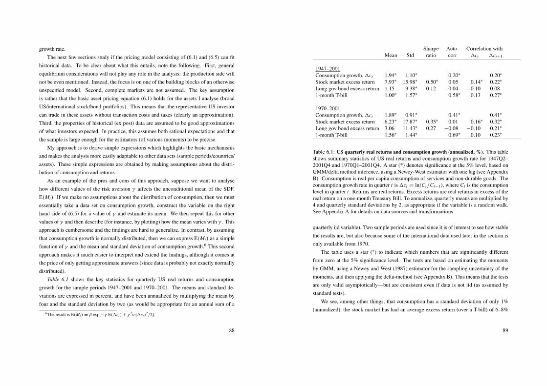
growth rate.The next few sections study if the pricing model consisting of (6.1) and (6.5) can fit

historical data. To be clear about what this entails, note the following. First, generalequilibrium considerations will not play any role in the analysis: the production side willnot be even mentioned. Instead, the focus is on one of the building blocks of an otherwiseunspecified model. Second, complete markets are not assumed. The key assumptionis rather that the basic asset pricing equation (6.1) holds for the assets I analyse (broadUS/international stock/bond portfolios). This means that the representative US investorcan trade in these assets without transaction costs and taxes (clearly an approximation).Third, the properties of historical (ex post) data are assumed to be good approximationsof what investors expected. In practice, this assumes both rational expectations and thatthe sample is large enough for the estimators (of various moments) to be precise.

My approach is to derive simple expressions which highlights the basic mechanismsand makes the analysis more easily adaptable to other data sets (sample periods/countries/assets). These simple expressions are obtained by making assumptions about the distri-bution of consumption and returns.

As an example of the pros and cons of this approach, suppose we want to analysehow different values of the risk aversion γ affects the unconditional mean of the SDF,E(Mt). If we make no assumptions about the distribution of consumption, then we mustessentially take a data set on consumption growth, construct the variable on the righthand side of (6.5) for a value of γ and estimate its mean. We then repeat this for othervalues of γ and then describe (for instance, by plotting) how the mean varies with γ . Thisapproach is cumbersome and the findings are hard to generalize. In contrast, by assumingthat consumption growth is normally distributed, then we can express E(Mt) as a simplefunction of γ and the mean and standard deviation of consumption growth.6 This secondapproach makes it much easier to interpret and extend the findings, although it comes atthe price of only getting approximate answers (since data is probably not exactly normallydistributed).

Table 6.1 shows the key statistics for quarterly US real returns and consumptiongrowth for the sample periods 1947–2001 and 1970–2001. The means and standard de-viations are expressed in percent, and have been annualized by multiplying the mean byfour and the standard deviation by two (as would be appropriate for an annual sum of a

6The result is E(Mt ) = β exp[−γ E(1ct )+ γ 2σ(1ct )2/2].

88

Sharpe Auto- Correlation withMean Std ratio corr 1ct 1ct+1

1947–2001Consumption growth, 1ct 1.94∗ 1.10∗ 0.20∗ 0.20∗

Stock market excess return 7.93∗ 15.98∗ 0.50∗ 0.05 0.14∗ 0.22∗

Long gov bond excess return 1.15 9.38∗ 0.12 −0.04 −0.10 0.081-month T-bill 1.00∗ 1.57∗ 0.58∗ 0.13 0.27∗

1970–2001Consumption growth, 1ct 1.89∗ 0.91∗ 0.41∗ 0.41∗

Stock market excess return 6.23∗ 17.87∗ 0.35∗ 0.01 0.16∗ 0.32∗

Long gov bond excess return 3.06 11.43∗ 0.27 −0.08 −0.10 0.21∗

1-month T-bill 1.56∗ 1.44∗ 0.69∗ 0.10 0.23∗

Table 6.1: US quarterly real returns and consumption growth (annualized, %). This tableshows summary statistics of US real returns and consumption growth rate for 1947Q2–2001Q4 and 1970Q1–2001Q4. A star (*) denotes significance at the 5% level, based onGMM/delta method inference, using a Newey-West estimator with one lag (see AppendixB). Consumption is real per capita consumption of services and non-durable goods. Theconsumption growth rate in quarter t is1ct = ln(Ct/Ct−1), where Ct is the consumptionlevel in quarter t . Returns are real returns. Excess returns are real returns in excess of thereal return on a one-month Treasury Bill. To annualize, quarterly means are multiplied by4 and quarterly standard deviations by 2, as appropriate if the variable is a random walk.See Appendix A for details on data sources and transformations.

quarterly iid variable). Two sample periods are used since it is of interest to see how stablethe results are, but also because some of the international data used later in the section isonly available from 1970.

The table uses a star (∗) to indicate which numbers that are significantly differentfrom zero at the 5% significance level. The tests are based on estimating the momentsby GMM, using a Newey and West (1987) estimator for the sampling uncertainty of themoments, and then applying the delta-method (see Appendix B). This means that the testsare only valid asymptotically—but are consistent even if data is not iid (as assumed bystandard tests).

We see, among other things, that consumption has a standard deviation of only 1%(annualized), the stock market has had an average excess return (over a T-bill) of 6–8%

89

(annualized), and that returns are only weakly correlated with consumption growth. Thesefigures will be important in the following sections. Two correlations with consumptiongrowth are shown, since it is unclear if returns should be related to what is recorded asconsumption this quarter or the next. The reason is that consumption is measured as aflow during the quarter, while returns are measured at the end of the quarter.

6.2.2 The Equity Premium Puzzle

This section studies if the consumption-based asset pricing model can explain the histor-ical risk premium on the US stock market.

To discuss the historical average excess returns, it is convenient to work with theunconditional pricing equation E(Rt Mt) = 1, which follows from applying the law ofiterated expectations on (6.1). We can then derive expressions like (6.2)–(6.4) for uncon-ditional moments instead.

To highlight the basic problem with the consumption-based model and to simplify theexposition, I assume that the excess return, Re

t , and the log SDF, ln(Mt), have a bivariatenormal distribution.7 Stein’s lemma8 then gives

Cov(Ret ,Mt) = Cov[Re

t , ln(Mt)] × E(Mt). (6.7)

We use this in the unconditional version of (6.4) to get the excess return and Sharpe ratioas

E(Ret ) = − Cov[Re

t , ln(Mt)], and (6.8)

E(Ret )/σ (R

et ) = −ρ[Re

t , ln(Mt)] × σ [ln(Mt)], (6.9)

where ρ[Ret , ln(Mt)] is the correlation of the excess return and the log SDF, and σ(Re

t )

and σ [ln(Mt)] are the standard deviations of the excess return and log SDF respectively.The log SDF in (6.6) is linear in consumption growth so the assumption of normality

boils down to assuming that Ret and1ct have a bivariate normal distribution. We can then

7This does not imply (but is implied by) normally distributed gross returns, which would eventuallyviolate limited liability. Even so, that would only happen once every 3000 years or so with the means andvolatilities in Table 6.1. I just wonder if Psusennes I (Pharao 1044BC to 994BC) allowed limited liability.In any case, his gold mask (Egyptian Museum, Cairo) is second only to Tutanchamon’s.

8Stein’s lemma says that if x and y have a bivariate normal distribution and h(y) is a differentiablefunction such that E[|h′(y)|] < ∞, then Cov[x, h(y)] = Cov(x, y)E[h′(y)]. This holds also for conditionaldistributions. In (6.7), x = Re

t , y = ln(Mt ), and h(y) = exp(y) so h′(y) = Mt .

90

write (6.8)–(6.9) as

E(Ret ) = Cov(Re

t ,1ct)γ , and (6.10)

E(Ret )/σ (R

et ) = ρ(Re

t ,1ct)× σ(1ct)γ, (6.11)

This expression is convenient since it allows us to split the Sharpe ratio into threeseparate factors: the correlation of returns and consumption growth, the volatility of con-sumption growth, and the risk aversion. In particular, the first two factors can be estimateddirectly from data without knowing any preference parameters and the volatility is a con-stant in a cross-section (something we will use later).

Equation (6.11) shows that to get a positive expected excess return, the asset must be“risky” in the sense that it is positively correlated with consumption growth (negativelycorrelated with the SDF). In that case, the asset tends to give a high return when marginalutility is low, so investors demand a risk premium. This effect is strong if consumption isvery volatile and/or investors are strongly risk averse.

Table 6.1 shows that the stock market has a Sharpe ratio around 0.35–0.5 (annualized)and that the consumption growth rate has a standard deviation of around 1% = 0.01(annualized). The lowest value of γ which makes equation (6.11) hold is then γ = 35,and this would only work if the stock market were a worthless hedge against consumptionfluctuations so the correlation is one.9

The basic problem with the consumption-based asset pricing model is that investorsenjoy a fairly stable consumption series (either because income is smooth or because it iseasy/inexpensive to smooth consumption by changing savings), so only an extreme riskaversion can motivate why investors require such a high equity premium. This is theequity premium puzzle stressed by Mehra and Prescott (1985) (although they approachthe issue from another angle—more about that later on).

Still higher values of γ are needed if the correlation in (6.11) is lower than one—asit certainly is. Table 6.1 shows that the correlation is around 0.1–0.3, where the highervalue is for the correlation with 1ct+1. If we want to be nice to the consumption-basedmodel, then we can use the higher value. With a Sharpe ratio of 0.35 (the lowest value,

9This is related to the approach in Hansen and Jagannathan (1991). Rewrite (6.4) as E(Ret )/σ (R

et ) =

−ρ(Ret ,Mt )σ (Mt )/E(Mt ), which shows that the following “volatility bound” must hold: σ(Mt )/E(Mt ) ≥

| E(Ret )|/σ(R

et ). Their approach is essentially to search in a set of returns for the portfolio with the largest

Sharpe ratio and then study if a given model of the SDF satisfies the volatility bound. In the case consideredhere there is only one asset.

91

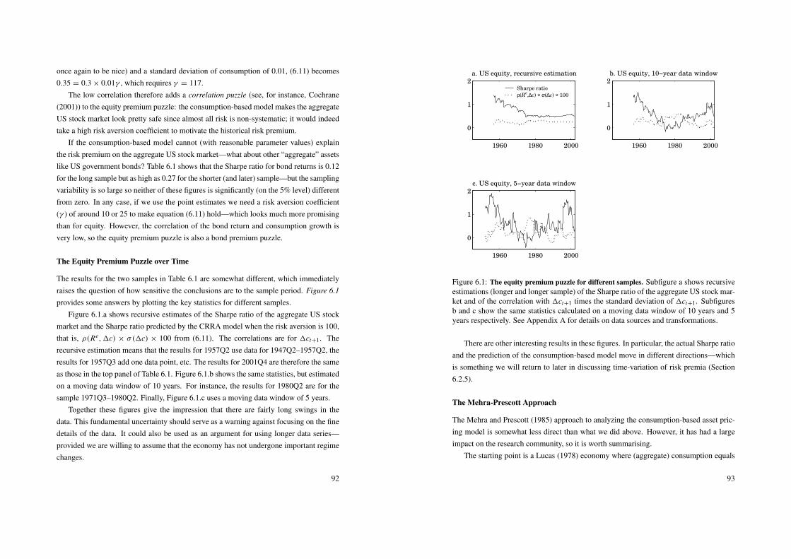
once again to be nice) and a standard deviation of consumption of 0.01, (6.11) becomes0.35 = 0.3 × 0.01γ , which requires γ = 117.

The low correlation therefore adds a correlation puzzle (see, for instance, Cochrane(2001)) to the equity premium puzzle: the consumption-based model makes the aggregateUS stock market look pretty safe since almost all risk is non-systematic; it would indeedtake a high risk aversion coefficient to motivate the historical risk premium.

If the consumption-based model cannot (with reasonable parameter values) explainthe risk premium on the aggregate US stock market—what about other “aggregate” assetslike US government bonds? Table 6.1 shows that the Sharpe ratio for bond returns is 0.12for the long sample but as high as 0.27 for the shorter (and later) sample—but the samplingvariability is so large so neither of these figures is significantly (on the 5% level) differentfrom zero. In any case, if we use the point estimates we need a risk aversion coefficient(γ ) of around 10 or 25 to make equation (6.11) hold—which looks much more promisingthan for equity. However, the correlation of the bond return and consumption growth isvery low, so the equity premium puzzle is also a bond premium puzzle.

The Equity Premium Puzzle over Time

The results for the two samples in Table 6.1 are somewhat different, which immediatelyraises the question of how sensitive the conclusions are to the sample period. Figure 6.1

provides some answers by plotting the key statistics for different samples.Figure 6.1.a shows recursive estimates of the Sharpe ratio of the aggregate US stock

market and the Sharpe ratio predicted by the CRRA model when the risk aversion is 100,that is, ρ(Re,1c) × σ(1c) × 100 from (6.11). The correlations are for 1ct+1. Therecursive estimation means that the results for 1957Q2 use data for 1947Q2–1957Q2, theresults for 1957Q3 add one data point, etc. The results for 2001Q4 are therefore the sameas those in the top panel of Table 6.1. Figure 6.1.b shows the same statistics, but estimatedon a moving data window of 10 years. For instance, the results for 1980Q2 are for thesample 1971Q3–1980Q2. Finally, Figure 6.1.c uses a moving data window of 5 years.

Together these figures give the impression that there are fairly long swings in thedata. This fundamental uncertainty should serve as a warning against focusing on the finedetails of the data. It could also be used as an argument for using longer data series—provided we are willing to assume that the economy has not undergone important regimechanges.

92

1960 1980 2000

0

1

2a. US equity, recursive estimation

Sharpe ratio

ρ(Re,∆c) × σ(∆c) × 100

1960 1980 2000

0

1

2b. US equity, 10−year data window

1960 1980 2000

0

1

2c. US equity, 5−year data window

Figure 6.1: The equity premium puzzle for different samples. Subfigure a shows recursiveestimations (longer and longer sample) of the Sharpe ratio of the aggregate US stock mar-ket and of the correlation with 1ct+1 times the standard deviation of 1ct+1. Subfiguresb and c show the same statistics calculated on a moving data window of 10 years and 5years respectively. See Appendix A for details on data sources and transformations.

There are other interesting results in these figures. In particular, the actual Sharpe ratioand the prediction of the consumption-based model move in different directions—whichis something we will return to later in discussing time-variation of risk premia (Section6.2.5).

The Mehra-Prescott Approach

The Mehra and Prescott (1985) approach to analyzing the consumption-based asset pric-ing model is somewhat less direct than what we did above. However, it has had a largeimpact on the research community, so it is worth summarising.

The starting point is a Lucas (1978) economy where (aggregate) consumption equals

93

the exogenous (aggregate) endowment. To see how this works, write the gross return asRt = (Pt + Dt)/Pt−1, where Pt is the asset price and Dt the dividend (per asset) in periodt . We can then write (6.1) as Pt−1 = Et−1[Mt(Pt + Dt)]. Iterating forward, applying thelaw of iterated expectations, ruling out bubbles, and using the CRRA SDF in (6.5) give

Pt−1 = Et−1[β(Ct/Ct−1)

−γ Dt + β2(Ct+1/Ct−1)−γ Dt+1 + . . .

]. (6.12)

The price of a real one-period bond is found by setting Dt = 1 and all future dividendsto zero. The price of a claim to the stream of future non-storable endowments—which isinterpreted as a proxy of a broad stock market index—is found by setting Dt equal to Ct .With a time series process for consumption, and values of β and γ , it is straightforwardto calculate asset returns.

Mehra and Prescott (1985) construct a time series process by postulating that con-sumption growth follows a two-state Markov process: Ct/Ct−1 is either low or high andthe probability of which depends on whether Ct−1/Ct−2 was low or high. This makesit very simple to calculate the expectations in (6.12): there is only one state variable andit can only take two values. In spite of this, the process allows both autocorrelation andtime-varying volatility. The model parameters are calibrated to fit the mean, standarddeviation, and autocorrelation in consumption growth. With this machinery, Mehra andPrescott (1985) find that a very high value of γ is needed to explain the historical equitypremium—basically because consumption is fairly smooth.

This approach is interesting, but it is a fairly indirect method for studying the equitypremium, and it adds a few very strong assumptions, in particular, about the consump-tion process and that the stockmarket corresponds to a claim on future consumption. Inany case, several extensions have been made, for instance to investigate if more extremeconsumption growth processes (fat tails or “crash states”) can rescue the model—but sofar with limited success (see, for instance, Salyer (1998) and Bidarkota and McCulloch(2003)).

6.2.3 The Riskfree Rate Puzzle

The CRRA utility function has the special feature that the intertemporal elasticity of sub-stitution is the inverse of the risk aversion, that is, 1/γ . The choice of the risk aversionparameter, for instance, to fit the equity premium, will therefore have direct effects on the

94

riskfree rate.A key feature of any consumption-based asset pricing model, or any consumption/saving

model for that matter, is that the riskfree rate governs the time slope of the consumptionprofile. From the asset pricing equation for a riskfree asset (6.3) we have Et−1(R f t)Et−1(Mt) =

1, which in the CRRA model becomes

Et−1(R f t)Et−1[β(Ct/Ct−1)−γ

] = 1. (6.13)

Note that we must use the conditional asset pricing equation —at least as long as webelieve that the riskfree asset is a random variable. A riskfree asset is defined by havinga zero conditional covariance with the SDF, which means that it is regarded as riskfreeat the time of investment (t − 1). In practice, this means a real interest rate (perhapsapproximated by the real return on a T-bill since the innovations in inflation are small),which may well have a nonzero unconditional covariance with the SDF.10 Indeed, in Table6.1 the real return on a T-bill is as correlated with consumption growth as the aggregateUS stockmarket.

To make progress, assume that the log SDF and the log riskfree rate r f t = ln(R f t)

have a bivariate normal distribution—which is somewhat different from our earlier as-sumption, but should (once again) be seen as just a an approximation. We can then write(6.13) as11

Et−1(r f t)+ σ 2t−1(r f t)/2 = − ln(β)+ γ Et−1(1ct)− γ 2σ 2

t−1(1ct)/2. (6.14)

To relate this equation to historical data, we take unconditional expectations to get

E(r f t)+ E σ 2t−1(r f t)/2 = − ln(β)+ γ E(1ct)− γ 2 E σ 2

t−1(1ct)/2. (6.15)

Before we try to compare (6.15) with data, several things should be noted. First, thelog gross rate is very close to a traditional net rate (ln(1 + z) ≈ z for small z), so it makessense to compare with the data in Table 6.1. Second, we can safely disregard the varianceterms since they are very small, at least as long as we are considering reasonable values ofγ . Although the average conditional variances are not directly observable, we know that

10As a very simple example, let xt = zt−1 +εt and yt = zt−1 +ut where εt are ut uncorrelated with eachother and with zt−1. If zt−1 is observable in t − 1, then Covt−1(xt , yt ) = 0, but Cov(xt , yt ) = σ 2(zt−1).

11If x ∼ N (µ, σ 2) and y = exp(x) then E(yk) = exp(kµ+ k2σ 2/2).

95

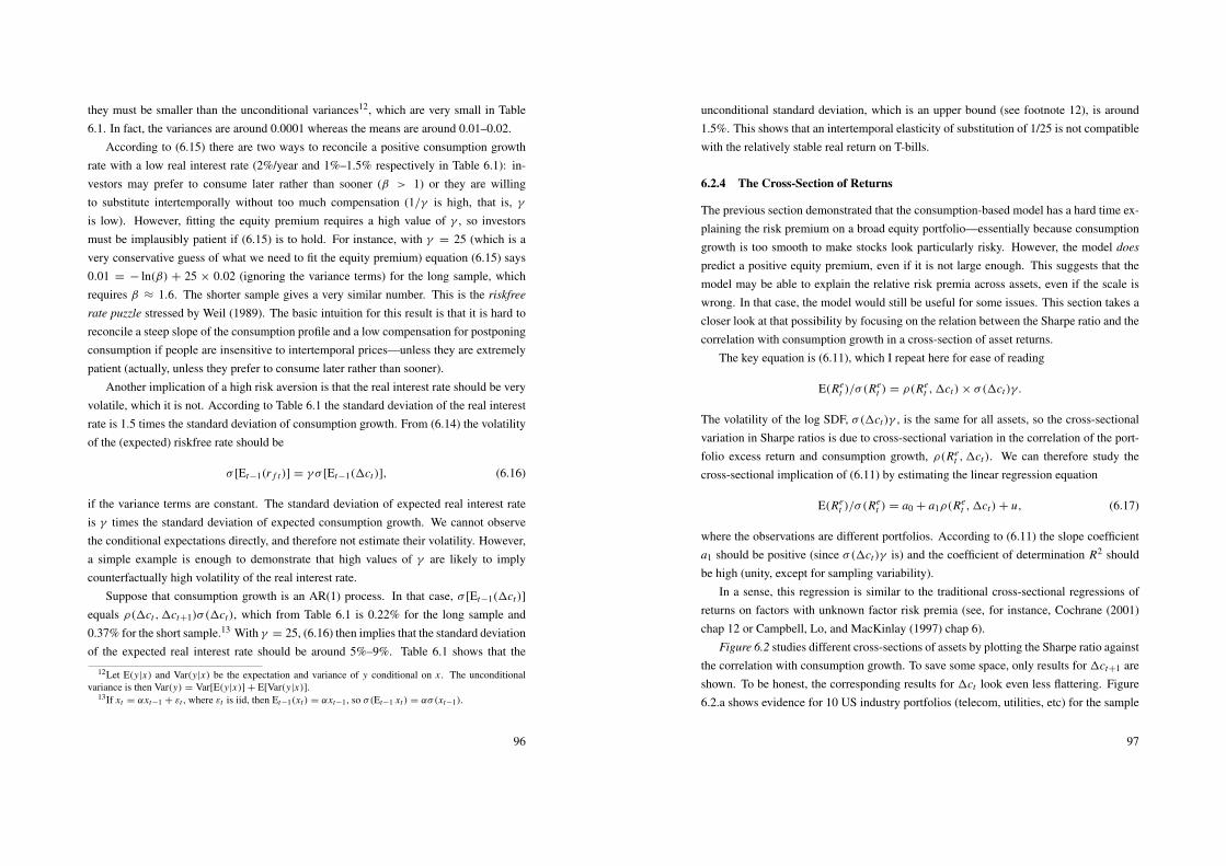
they must be smaller than the unconditional variances12, which are very small in Table6.1. In fact, the variances are around 0.0001 whereas the means are around 0.01–0.02.

According to (6.15) there are two ways to reconcile a positive consumption growthrate with a low real interest rate (2%/year and 1%–1.5% respectively in Table 6.1): in-vestors may prefer to consume later rather than sooner (β > 1) or they are willingto substitute intertemporally without too much compensation (1/γ is high, that is, γis low). However, fitting the equity premium requires a high value of γ , so investorsmust be implausibly patient if (6.15) is to hold. For instance, with γ = 25 (which is avery conservative guess of what we need to fit the equity premium) equation (6.15) says0.01 = − ln(β) + 25 × 0.02 (ignoring the variance terms) for the long sample, whichrequires β ≈ 1.6. The shorter sample gives a very similar number. This is the riskfree

rate puzzle stressed by Weil (1989). The basic intuition for this result is that it is hard toreconcile a steep slope of the consumption profile and a low compensation for postponingconsumption if people are insensitive to intertemporal prices—unless they are extremelypatient (actually, unless they prefer to consume later rather than sooner).

Another implication of a high risk aversion is that the real interest rate should be veryvolatile, which it is not. According to Table 6.1 the standard deviation of the real interestrate is 1.5 times the standard deviation of consumption growth. From (6.14) the volatilityof the (expected) riskfree rate should be

σ [Et−1(r f t)] = γ σ [Et−1(1ct)], (6.16)

if the variance terms are constant. The standard deviation of expected real interest rateis γ times the standard deviation of expected consumption growth. We cannot observethe conditional expectations directly, and therefore not estimate their volatility. However,a simple example is enough to demonstrate that high values of γ are likely to implycounterfactually high volatility of the real interest rate.

Suppose that consumption growth is an AR(1) process. In that case, σ [Et−1(1ct)]

equals ρ(1ct ,1ct+1)σ (1ct), which from Table 6.1 is 0.22% for the long sample and0.37% for the short sample.13 With γ = 25, (6.16) then implies that the standard deviationof the expected real interest rate should be around 5%–9%. Table 6.1 shows that the

12Let E(y|x) and Var(y|x) be the expectation and variance of y conditional on x . The unconditionalvariance is then Var(y) = Var[E(y|x)] + E[Var(y|x)].

13If xt = αxt−1 + εt , where εt is iid, then Et−1(xt ) = αxt−1, so σ(Et−1 xt ) = ασ(xt−1).

96

unconditional standard deviation, which is an upper bound (see footnote 12), is around1.5%. This shows that an intertemporal elasticity of substitution of 1/25 is not compatiblewith the relatively stable real return on T-bills.

6.2.4 The Cross-Section of Returns

The previous section demonstrated that the consumption-based model has a hard time ex-plaining the risk premium on a broad equity portfolio—essentially because consumptiongrowth is too smooth to make stocks look particularly risky. However, the model does

predict a positive equity premium, even if it is not large enough. This suggests that themodel may be able to explain the relative risk premia across assets, even if the scale iswrong. In that case, the model would still be useful for some issues. This section takes acloser look at that possibility by focusing on the relation between the Sharpe ratio and thecorrelation with consumption growth in a cross-section of asset returns.

The key equation is (6.11), which I repeat here for ease of reading

E(Ret )/σ (R

et ) = ρ(Re

t ,1ct)× σ(1ct)γ.

The volatility of the log SDF, σ(1ct)γ , is the same for all assets, so the cross-sectionalvariation in Sharpe ratios is due to cross-sectional variation in the correlation of the port-folio excess return and consumption growth, ρ(Re

t ,1ct). We can therefore study thecross-sectional implication of (6.11) by estimating the linear regression equation

E(Ret )/σ (R

et ) = a0 + a1ρ(Re

t ,1ct)+ u, (6.17)

where the observations are different portfolios. According to (6.11) the slope coefficienta1 should be positive (since σ(1ct)γ is) and the coefficient of determination R2 shouldbe high (unity, except for sampling variability).

In a sense, this regression is similar to the traditional cross-sectional regressions ofreturns on factors with unknown factor risk premia (see, for instance, Cochrane (2001)chap 12 or Campbell, Lo, and MacKinlay (1997) chap 6).

Figure 6.2 studies different cross-sections of assets by plotting the Sharpe ratio againstthe correlation with consumption growth. To save some space, only results for 1ct+1 areshown. To be honest, the corresponding results for 1ct look even less flattering. Figure6.2.a shows evidence for 10 US industry portfolios (telecom, utilities, etc) for the sample

97

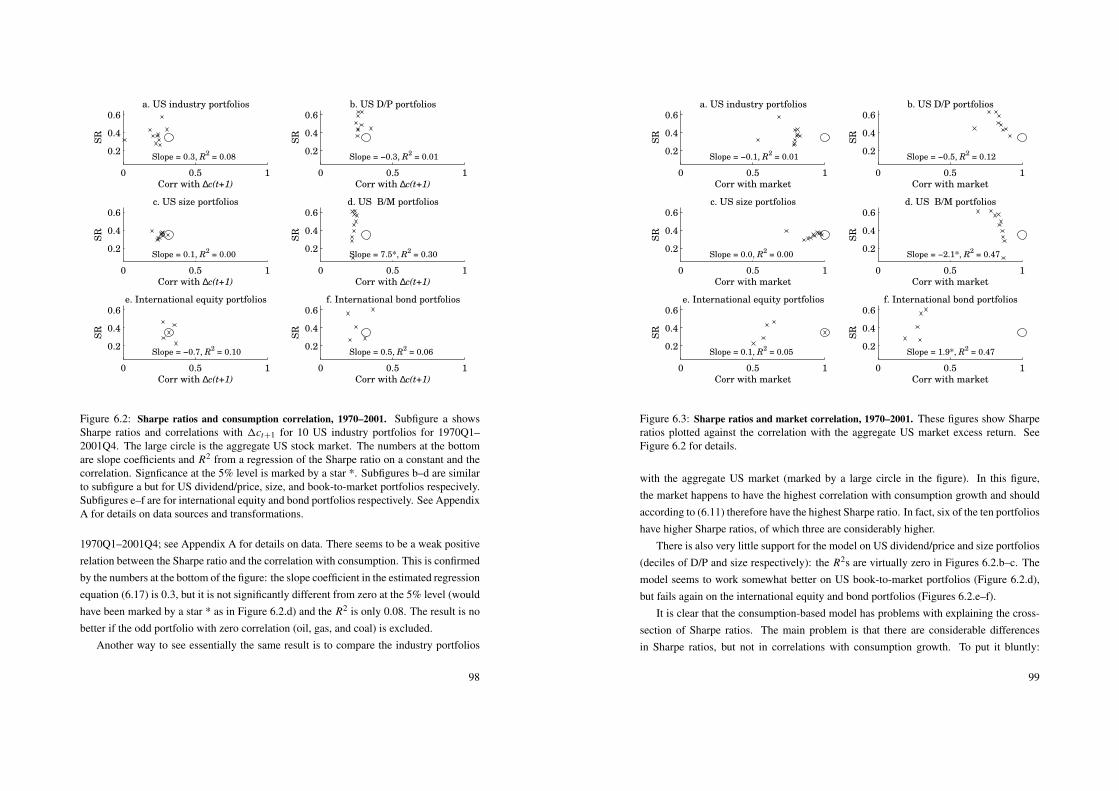
0 0.5 1

0.2

0.4

0.6a. US industry portfolios

Corr with ∆c(t+1)

SR

Slope = 0.3, R2 = 0.08

0 0.5 1

0.2

0.4

0.6b. US D/P portfolios

Corr with ∆c(t+1)

SR

Slope = −0.3, R2 = 0.01

0 0.5 1

0.2

0.4

0.6c. US size portfolios

Corr with ∆c(t+1)

SR

Slope = 0.1, R2 = 0.00

0 0.5 1

0.2

0.4

0.6d. US B/M portfolios

Corr with ∆c(t+1)

SR

Slope = 7.5*, R2 = 0.30

0 0.5 1

0.2

0.4

0.6e. International equity portfolios

Corr with ∆c(t+1)

SR

Slope = −0.7, R2 = 0.10

0 0.5 1

0.2

0.4

0.6f. International bond portfolios

Corr with ∆c(t+1)

SR

Slope = 0.5, R2 = 0.06

Figure 6.2: Sharpe ratios and consumption correlation, 1970–2001. Subfigure a showsSharpe ratios and correlations with 1ct+1 for 10 US industry portfolios for 1970Q1–2001Q4. The large circle is the aggregate US stock market. The numbers at the bottomare slope coefficients and R2 from a regression of the Sharpe ratio on a constant and thecorrelation. Signficance at the 5% level is marked by a star *. Subfigures b–d are similarto subfigure a but for US dividend/price, size, and book-to-market portfolios respecively.Subfigures e–f are for international equity and bond portfolios respectively. See AppendixA for details on data sources and transformations.

1970Q1–2001Q4; see Appendix A for details on data. There seems to be a weak positiverelation between the Sharpe ratio and the correlation with consumption. This is confirmedby the numbers at the bottom of the figure: the slope coefficient in the estimated regressionequation (6.17) is 0.3, but it is not significantly different from zero at the 5% level (wouldhave been marked by a star * as in Figure 6.2.d) and the R2 is only 0.08. The result is nobetter if the odd portfolio with zero correlation (oil, gas, and coal) is excluded.

Another way to see essentially the same result is to compare the industry portfolios

98

0 0.5 1

0.2

0.4

0.6a. US industry portfolios

Corr with market

SR

Slope = −0.1, R2 = 0.01

0 0.5 1

0.2

0.4

0.6b. US D/P portfolios

Corr with market

SR

Slope = −0.5, R2 = 0.12

0 0.5 1

0.2

0.4

0.6c. US size portfolios

Corr with market

SR

Slope = 0.0, R2 = 0.00

0 0.5 1

0.2

0.4

0.6d. US B/M portfolios

Corr with market

SR

Slope = −2.1*, R2 = 0.47

0 0.5 1

0.2

0.4

0.6e. International equity portfolios

Corr with market

SR

Slope = 0.1, R2 = 0.05

0 0.5 1

0.2

0.4

0.6f. International bond portfolios

Corr with market

SR

Slope = 1.9*, R2 = 0.47

Figure 6.3: Sharpe ratios and market correlation, 1970–2001. These figures show Sharperatios plotted against the correlation with the aggregate US market excess return. SeeFigure 6.2 for details.

with the aggregate US market (marked by a large circle in the figure). In this figure,the market happens to have the highest correlation with consumption growth and shouldaccording to (6.11) therefore have the highest Sharpe ratio. In fact, six of the ten portfolioshave higher Sharpe ratios, of which three are considerably higher.

There is also very little support for the model on US dividend/price and size portfolios(deciles of D/P and size respectively): the R2s are virtually zero in Figures 6.2.b–c. Themodel seems to work somewhat better on US book-to-market portfolios (Figure 6.2.d),but fails again on the international equity and bond portfolios (Figures 6.2.e–f).

It is clear that the consumption-based model has problems with explaining the cross-section of Sharpe ratios. The main problem is that there are considerable differencesin Sharpe ratios, but not in correlations with consumption growth. To put it bluntly:

99

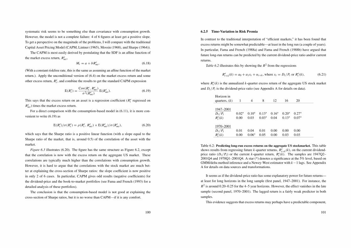
systematic risk seems to be something else than covariance with consumption growth.However, the model is not a complete failure: 4 of 6 figures at least get a positive slope.To get a perspective on the magnitude of the problems, I will compare with the traditionalCapital Asset Pricing Model (CAPM, Lintner (1965), Mossin (1968), and Sharpe (1964)).

The CAPM is most easily derived by postulating that the SDF is an affine function ofthe market excess return, Re

mt ,Mt = a + bRe

mt . (6.18)

(With a constant riskfree rate, this is the same as assuming an affine function of the marketreturn.). Apply the unconditional version of (6.4) on the market excess return and someother excess return, Re

t , and combine the results to get the standard CAPM expression

E(Ret ) =

Cov(Ret , Re

mt)

σ 2(Remt)

E(Remt). (6.19)

This says that the excess return on an asset is a regression coefficient (Ret regressed on

Remt ) times the market excess return.

For a direct comparison with the consumption-based model in (6.11), it is more con-venient to write (6.19) as

E(Ret )/σ (R

et ) = ρ(Re

t , Remt)× E(Re

mt)/σ (Remt), (6.20)

which says that the Sharpe ratio is a positive linear function (with a slope equal to theSharpe ratio of the market, that is, around 0.5) of the correlation of the asset with themarket.

Figure 6.3 illustrates (6.20). The figure has the same structure as Figure 6.2, exceptthat the correlation is now with the excess return on the aggregate US market. Thesecorrelations are typically much higher than the correlations with consumption growth.However, it is hard to argue that the correlations with the stock market are much bet-ter at explaining the cross-section of Sharpe ratios: the slope coefficient is now positivein only 2 of 6 cases. In particular, CAPM gives odd results (negative coefficients) forthe dividend-price and the book-to-market portfolios (see Fama and French (1993) for adetailed analysis of these portfolios).

The conclusion is that the consumption-based model is not good at explaining thecross-section of Sharpe ratios, but it is no worse than CAPM—if it is any comfort.

100

6.2.5 Time-Variation in Risk Premia

In contrast to the traditional interpretation of “efficient markets,” it has been found thatexcess returns might be somewhat predictable—at least in the long run (a couple of years).In particular, Fama and French (1988a) and Fama and French (1988b) have argued thatfuture long-run returns can be predicted by the current dividend-price ratio and/or currentreturns.

Table 6.2 illustrates this by showing the R2 from the regressions

Ret+k(k) = a0 + a1xt + ut+k , where xt = Dt/Pt or Re

t (k), (6.21)

where Ret (k) is the annualized k-quarter excess return of the aggregate US stock market

and Dt/Pt is the dividend-price ratio (see Appendix A for details on data).

Horizon inquarters, (k) 1 4 8 12 16 20

1947–2001Dt/Pt 0.02∗ 0.10∗ 0.13∗ 0.16∗ 0.20∗ 0.27∗

Ret (k) 0.00 0.03 0.03∗ 0.04 0.13∗ 0.07∗

1970–2001Dt/Pt 0.01 0.04 0.01 0.00 0.00 0.00Re

t (k) 0.00 0.06∗ 0.05 0.00 0.03 0.03

Table 6.2: Predicting long-run excess returns on the aggregate US stockmarket. This tableshows results from regressing future k-quarter returns, Re

t+k(k), on the current dividend-price ratio (Dt/Pt ) or the current k-quarter return, Re

t (k). The samples are 1947Q2–2001Q4 and 1970Q1–2001Q4. A star (*) denotes a significance at the 5% level, based onGMM/delta method inference and a Newey-West estimator with k −1 lags. See AppendixA for details on data sources and transformations.

It seems as if the dividend-price ratio has some explanatory power for future returns—at least for long horizons in the long sample (first panel, 1947–2001). For instance, theR2 is around 0.20–0.25 for the 4–5 year horizons. However, the effect vanishes in the latesample (second panel, 1970–2001). The lagged return is a fairly weak predictor in bothsamples.

This evidence suggests that excess returns may perhaps have a predictable component,

101

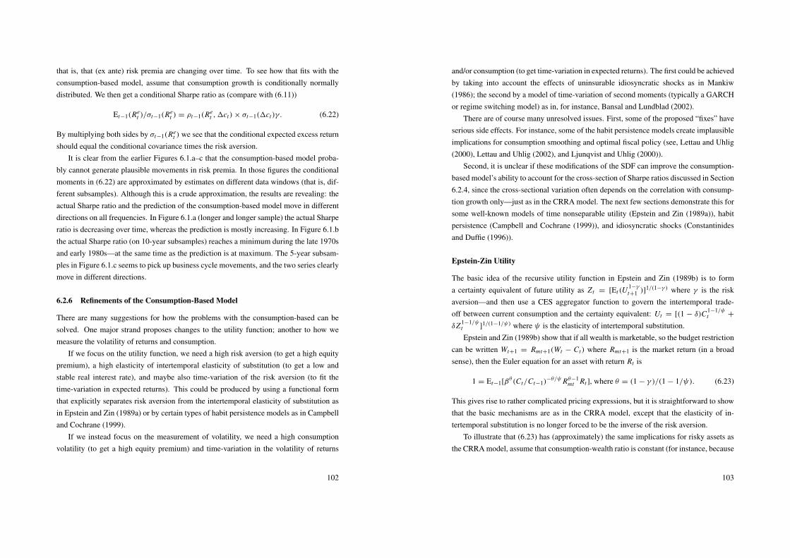
that is, that (ex ante) risk premia are changing over time. To see how that fits with theconsumption-based model, assume that consumption growth is conditionally normallydistributed. We then get a conditional Sharpe ratio as (compare with (6.11))

Et−1(Ret )/σt−1(Re

t ) = ρt−1(Ret ,1ct)× σt−1(1ct)γ. (6.22)

By multiplying both sides by σt−1(Ret ) we see that the conditional expected excess return

should equal the conditional covariance times the risk aversion.It is clear from the earlier Figures 6.1.a–c that the consumption-based model proba-

bly cannot generate plausible movements in risk premia. In those figures the conditionalmoments in (6.22) are approximated by estimates on different data windows (that is, dif-ferent subsamples). Although this is a crude approximation, the results are revealing: theactual Sharpe ratio and the prediction of the consumption-based model move in differentdirections on all frequencies. In Figure 6.1.a (longer and longer sample) the actual Sharperatio is decreasing over time, whereas the prediction is mostly increasing. In Figure 6.1.bthe actual Sharpe ratio (on 10-year subsamples) reaches a minimum during the late 1970sand early 1980s—at the same time as the prediction is at maximum. The 5-year subsam-ples in Figure 6.1.c seems to pick up business cycle movements, and the two series clearlymove in different directions.

6.2.6 Refinements of the Consumption-Based Model

There are many suggestions for how the problems with the consumption-based can besolved. One major strand proposes changes to the utility function; another to how wemeasure the volatility of returns and consumption.

If we focus on the utility function, we need a high risk aversion (to get a high equitypremium), a high elasticity of intertemporal elasticity of substitution (to get a low andstable real interest rate), and maybe also time-variation of the risk aversion (to fit thetime-variation in expected returns). This could be produced by using a functional formthat explicitly separates risk aversion from the intertemporal elasticity of substitution asin Epstein and Zin (1989a) or by certain types of habit persistence models as in Campbelland Cochrane (1999).

If we instead focus on the measurement of volatility, we need a high consumptionvolatility (to get a high equity premium) and time-variation in the volatility of returns

102

and/or consumption (to get time-variation in expected returns). The first could be achievedby taking into account the effects of uninsurable idiosyncratic shocks as in Mankiw(1986); the second by a model of time-variation of second moments (typically a GARCHor regime switching model) as in, for instance, Bansal and Lundblad (2002).

There are of course many unresolved issues. First, some of the proposed “fixes” haveserious side effects. For instance, some of the habit persistence models create implausibleimplications for consumption smoothing and optimal fiscal policy (see, Lettau and Uhlig(2000), Lettau and Uhlig (2002), and Ljunqvist and Uhlig (2000)).

Second, it is unclear if these modifications of the SDF can improve the consumption-based model’s ability to account for the cross-section of Sharpe ratios discussed in Section6.2.4, since the cross-sectional variation often depends on the correlation with consump-tion growth only—just as in the CRRA model. The next few sections demonstrate this forsome well-known models of time nonseparable utility (Epstein and Zin (1989a)), habitpersistence (Campbell and Cochrane (1999)), and idiosyncratic shocks (Constantinidesand Duffie (1996)).

Epstein-Zin Utility

The basic idea of the recursive utility function in Epstein and Zin (1989b) is to forma certainty equivalent of future utility as Z t = [Et(U

1−γ

t+1 )]1/(1−γ ) where γ is the risk

aversion—and then use a CES aggregator function to govern the intertemporal trade-off between current consumption and the certainty equivalent: Ut = [(1 − δ)C1−1/ψ

t +

δZ1−1/ψt ]

1/(1−1/ψ) where ψ is the elasticity of intertemporal substitution.Epstein and Zin (1989b) show that if all wealth is marketable, so the budget restriction

can be written Wt+1 = Rmt+1(Wt − Ct) where Rmt+1 is the market return (in a broadsense), then the Euler equation for an asset with return Rt is

1 = Et−1[βθ (Ct/Ct−1)

−θ/ψ Rθ−1mt Rt ], where θ = (1 − γ )/(1 − 1/ψ). (6.23)

This gives rise to rather complicated pricing expressions, but it is straightforward to showthat the basic mechanisms are as in the CRRA model, except that the elasticity of in-tertemporal substitution is no longer forced to be the inverse of the risk aversion.

To illustrate that (6.23) has (approximately) the same implications for risky assets asthe CRRA model, assume that consumption-wealth ratio is constant (for instance, because

103

the market return is iid). This effectively closes down all interaction between the risk andintertemporal substitution (see Svensson (1989) and Campbell (1993)). It follows fromthe budget constraint that consumption growth and the market return are proportional so(6.23) can be written

Et−1[(Ct/Ct−1)−γ Rt ] = constant, (6.24)

which is exactly the same as the CRRA model. The Epstein-Zin model therefore inheritsthe problem with explaining the cross-section of Sharpe ratios. This is also approximatelytrue when the consumption-wealth ratio is not too variable. Of course, if there are largepredictable movements in the market return, then it is no longer true.

To see that the intertemporal substitution is governed by the parameter ψ , close downall systematic risk by assuming that the market return is a riskfree rate (set Rmt = Rt =

R f t in (6.23)) and that log consumption and the log real interest rate, r f t , have a bivariatenormal distribution. We then get

Et−1(r f t)+ θσ 2t−1(r f t)/2 = − ln(β)+

1ψ

Et−1(1ct)−θ

ψ2σ2t−1(1ct)/2. (6.25)

This is the same relation between the real interest rate and consumption growth as inthe CRRA case (see (6.14))—except that the elasticity of intertemporal substitution is nolonger forced to be the inverse of the risk aversion.

This analysis shows that the Epstein-Zin model could help us to solve the riskfree ratepuzzle (since we have a separate parameter for the elasticity of intertemporal substitution),but it can probably not do much with the equity premium (unless we are willing to accepta very high risk aversion) or the cross-sectional variation in Sharpe ratios.

Habit Persistence

The utility function in the habit persistence model of Campbell and Cochrane (1999)has the same functional form as the CRRA model, but the argument is the differencebetween consumption and a habit level, Ct − X t , instead of just consumption. Variationin consumption and habit can both contribute to variation in marginal utility, which affectsasset prices.

Campbell and Cochrane (1999) parameterize the habit in terms of the “surplus ra-tio” St = (Ct − X t)/Ct , which measures how much aggregate consumption exceeds thehabit. Since this ratio is external to the investor, marginal utility becomes (Ct − X t)

−γ=

104

(Ct St)−γ . We can therefore write the log SDF as

ln(Mt) = ln(β)− γ (1st +1ct), (6.26)

where st is the log surplus ratio. The process for st is assumed to be a non-linear AR(1)

st = φst−1 + λ(st−1)1ct + constant, (6.27)

where λ(st−1) is a decreasing function of st−1 which controls the sensitivity to (aggregate)consumption growth. The function λ(st−1) is always non-negative, so the log surplus ratioreacts positively to consumption growth (the main effect of letting λ depend on st−1 is tomake the risk premium move with the business cycle). Because of (6.27), a move in 1ct

will typically be accompanied by a move of 1st in the same direction, which increasesthe volatility of the SDF (6.26). In other words, a move in consumption drives the habitX t in the opposite direction so Ct − X t varies a great deal.

Consumption growth is assumed to be conditionally normally distributed, so the con-ditional Sharpe ratio is (compare with (6.9))

Et−1(Ret )/σt−1(Re

t ) = −ρt−1[Ret , ln(Mt)] × σt−1[ln(Mt)]. (6.28)

From (6.26) and (6.27) we note that the innovation in the log SDF is −γ [λ(st−1) + 1]

times the innovation in 1ct . Since λ(st−1) is positive and known in t − 1 this is verysimilar to the CRRA model, except that the conditional volatility of the log SDF (the lastterm in (6.28)) is scaled up. This could help explain a higher risk premium. In a way,it is very similar to just increasing the risk aversion γ (although Campbell and Cochrane(1999) show that their model do not suffer from the some of the drawbacks of the CRRAmodel with a high γ ).

However, (6.28) has the same implication for the cross-sectional variation of Sharperatios as the CRRA model. The reason is that the conditional correlation in (6.28) isthe same as in the CRRA model since the innovation in the log SDF is proportional tothe innovation in consumption growth (and the factor of proportionality cancels in thecorrelation).

105

Idiosyncratic Risk

A quite different attempt to solve the problems with the consumption-based asset pricingmodel is to argue that aggregating individual investors into a (fictitious) representativeinvestor is a non-trivial task. Investors who face idiosyncratic risk that they cannot insureagainst (incomplete markets) may be reluctant to hold risky assets. Since macro dataaverages out idiosyncratic components, the volatility of aggregate consumption wouldthen underestimate true consumption volatility of a representative investor.

However, it is surprisingly hard to make this story stick. The first problem is that onlyshocks that cannot be hedged qualify as idiosyncratic shocks: hedging means averagingout. One way of hedging consumption (if not income) is to have a savings account (seeTelmer (1993)). Moreover, income can sometimes be partially hedged by trading in ex-isting assets if they are correlated with income. In practice, this means that idiosyncraticshocks are probably a quite smaller than the income shocks estimated from micro data.

The second problem is that idiosyncratic shocks may still not matter unless their dis-tribution is strongly tied to state of the economy. To develop an example, note that thebasic asset pricing equation (6.1) must hold for every investor (after all, it is his first ordercondition), so Et−1(Rt M j t) = 1 where M j t is the SDF of investor j . The conditional ver-sion of the asset pricing equation with normally distributed consumption growth (6.10)for investor j is then

Et−1(Ret ) = Covt−1(Re

t ,1c j t)γ, (6.29)

where 1c j t is consumption growth of investor j .We let the innovation in the consumption investor j have two components: an aggre-

gate innovation (common to all investors) and an idiosyncratic innovation. The idiosyn-cratic shock cannot be correlated with existing assets (discussed above), so it contributesnothing to the conditional covariance in (6.29): the risk premium will only depend onthe covariance of the return with the aggregate innovation—as in the CRRA model. Inthis case the idiosyncratic shocks do not matter for the risk premium (although they willtypically decrease the real interest rate as investors increase the precautionary saving).

This result is quite general. For instance, it holds for the Campbell and Cochrane(1999) model discussed before, and in any other model with a lognormal SDF where theidiosyncratic component affects the log SDF linearly (this follows directly from (6.8)).14

14Lettau (2002) shows that this property holds for any distribution of the consumption innovation if utility

106

To make idiosyncratic shocks matter for risk premia, they will either have to be some-thing less than completely idiosyncratic (for instance, affecting a group of investors whocollectively have market power; see Den Haan (2001)) or their distribution must dependon the aggregate shock (see Mankiw (1986) and Constantinides and Duffie (1996)).

In the latter class of models, a higher risk premium requires that the volatility ofthe idiosyncratic shocks is stochastic and that the innovations to this volatility and ofaggregate consumption are negatively correlated: bad times mean more risk. To illustratethis, consider the CRRA model where the log SDF for investor j is

ln(M j t) = ln(β)− γ1c j t . (6.30)

Let the innovation in consumption growth for investor j be

1c j t − Et−1(1c j t) = εt + u j t , (6.31)

where εt is the aggregate component and u j t the individual component which has a vari-ance which depends on the realization of εt .

With (6.30)–(6.31) the asset pricing equation for investor j says that

0 = Et−1(Ret M j t) (6.32)

= ER,ε,u{

Ret exp

[ln(β)− γ Et−1(1ct)− γ εt − γ u j t

]}. (6.33)

The operator ER,ε,u is used instead of Et−1 to indicate that the expectations involvesintegrating over the random variables Re

t , εt , and u j t . Suppose that the distribution ofu j t conditional on the aggregate innovation, εt , is normal with zero mean and variancevt−1 + λ(εt) where vt−1 is known in t − 1 and λ(εt) depends on the aggregate shock.Integrating over u j t then gives

0 = ER,ε{

Ret exp

[ln(β)− γ Et−1(1ct)+ γ 2vt−1 − γ εt + γ 2λ(εt)/2

]}, (6.34)

where ER,ε indicates that we now need to integrate over Ret and εt . (This first integration

works since the asset return is independent of the realization of the idiosyncratic shock,even if not of its variance.)

I follow the

is CRRA and the the distribution of the idiosyncratic component is not affected by the aggregate shock.

107

approximation in Lettau (2002) of assuming that εt and λ(εt) have a bivariate normaldistribution. This is only an approximation since it does not rule out negative variances,but it has the advantage of giving a very straightforward expression. The term in squarebrackets in (6.34) can then be interpreted as a normally distributed log SDF of the investor,which allows us to use the decomposition of the Sharpe ratio in (6.28) which I repeat herefor easy of reading

Et−1(Ret )/σt−1(Re

t ) = −ρt−1[Ret , ln(Mt)] × σt−1[ln(Mt)].

In this model, the conditional volatility and correlation are

σt−1[ln Mt)] = γ σt−1[εt − γ λ(εt)/2] (6.35)

−ρt−1[Ret , ln(Mt)] = ρt−1[Re

t , εt − γ λ(εt)/2]. (6.36)

Note that setting λ(εt)= 0 gives the same expressions as without idiosyncratic shocks. Infact, if λ(εt) is a constant, that is, if the volatility of the idiosyncratic shocks do not dependon the aggregate shock, then we also get the same expressions as without idiosyncraticshocks.

If λ(εt) is decreasing in εt so idiosyncratic risk is larger in bad times, then the volatil-ity in (6.35) is larger than without idiosyncratic shocks. This could help explaining theequity premium puzzle—although there are doubts about whether the idiosyncratic risk issufficiently volatile to be quantitatively important (see Lettau (2002) and Cogley (1998)).

However, this mechanism is unlikely to help the model to explain the cross-sectionalvariation in Sharpe ratios—which depends only on the correlation (6.36): as a first-orderapproximation this correlation is the same as when λ(εt) is constant. For instance, ifλ(εt) = a+bεt with b < 0, then this is exactly so. This gives the same implications for thecross-sectional dispersion of Sharpe ratios as the model without idiosyncratic shocks—at least unless the idiosyncratic dispersion is a very non-linear function of the aggregatestate.

An additional aspect of models with idiosyncratic risk is that they allow us to study theeffects of transaction costs in a serious way: heterogenous agents with idiosyncratic coststrade, representative agents do not. The first effect of transaction costs is to transform thefirst order condition of an investor to a set of inequalities 1/(1 + τ) ≤ Et−1(Rt M j t) ≤

1 + τ where τ is the (proportional) cost of a round-trip (the upper limit is for buying the

108

asset in t − 1 and selling in t ; the lower limit is for the opposite). This has been usedto modify the Hansen and Jagannathan (1991) bounds (see He and Modest (1995) andLuttmer (1996)) with mixed results. One of the key assumptions in that analysis seemsto be the assumption length of the period: a 0.5% transaction cost is quite substantivecompared to a 1% monthly (expected) return, but small compared to a 12% annual return.We therefore need to find the equilibrium (including the endogenous trading frequency)in order to analyse the importance of transaction costs. So far, the findings indicate thatthe effect on prices is relatively small (unless borrowing/lending is very costly) but thatthe effect on turnover is large (see Heaton and Lucas (1996) and Vayanos (1998)).

6.3 Assets in Simulation Models

This part of the chapter discusses how different types of assets are incorporated into sim-ulation models. The emphasis is on discussing the key properties of the assets when theyare priced by a consumption-based model.

I first analyse a number of different asset classes: short- and long-lived claims onaggregate consumption, options and levered claims, as well as short and long real/nominalinterest rates. To economise on space, I leave out some important asset classes like foreignexchange and real estate (see, for instance, Smith and Wickens (2002), Kollman (2001),Zimmermann (1999) and Hendershott (1998)). At the end, I discuss some other importantfeatures of how assets are modelled: time-variation in risk premia, the effect of non-Walrasian labour contracts, and the effect of adding an asset to an existing model.

The analysis has the same basic approach as in the first part of the chapter. First,the model consists of the basic asset pricing equation (6.1) and the consumption-basedstochastic discount factor (6.5). In practice, this means that we are studying equilibriumconditions on the joint behaviour of consumption growth and returns on assets that canbe freely traded. This does not assume that markets are complete. However, addingan asset to a model with incomplete markets may change the consumption process, sothe results we derive are only valid for assets that could be traded when the equilibriumwas determined (see Section 6.3.8 for a more detailed discussion). Second, analyticalpricing relations are derived by making assumptions about the distribution of returns andconsumption and sometimes also by approximating complicated expressions.

Although this approach is useful for providing intuition for how different types of

109

assets will work in a simulation model, it is clearly only a first step. In particular, thischapter never formulates and solves a full model. To do that, the other contributions tothis book, the references found below, and the text by Altug and Labadie (1994) shouldall be very useful.

6.3.1 Preliminaries

Many simulation models are close to log-linear and are typically fed with normally dis-tributed shocks. This means that most variables (including returns) are approximatelylognormally distributed—sometimes exactly so. I therefore derive new expressions forrisk premia and Sharpe ratios (the expressions in previous sections assumed normally,not lognormally, distributed returns). These expressions will be used repeatedly in thefollowing sections.

The asset pricing equation with the CRRA SDF is 1 = Et−1{β exp[−γ1ct + rt ]},where rt = ln(Rt) is the log return. If these variables have a bivariate normal distribution,it follows (see footnote 11) that the risk premium and Sharpe ratios are

Et−1(r et ) = Covt−1(γ1ct , r e

t ), and (6.37)

Et−1(r et )/σt−1(r e

t ) = ρt−1(1ct , r et )× σt−1(1ct)γ. (6.38)

The tilde is here to indicate that the risk premium is defined as Et−1(r et ) = Et−1(r e

t ) +

σ 2t−1(rt)/2, that is, the expected excess log return over the real interest rate, adjusted for

Jensen’s inequality. This definition of an excess return is perhaps slightly non-standard,but it captures all the aspects of interest here.

In the following sections I will make use of the fact that only innovations matter forthe risk premia, since it is only innovations that are risky. For the log excess return, thismeans that only the innovation in the risky asset payoff matters.15

6.3.2 Claims on Aggregate Consumption

This section analyses the pricing of claims on aggregate consumption. Many modelshave considered such assets—sometimes as an approximation of equity (see, for instance,Lucas (1978) and the references in Section 6.2.2). The main purpose of the discussion is

15The log excess return, ret is the log payoff minus the lagged log assset price (measured in real terms)

minus the log real interest rate. Only the first component has an innovation.

110

to highlight that the risk premium on long-lived consumption claims depends crucially onthe autocorrelation of consumption growth.

We first discuss a one-period claim and then move on to multiperiod claims. The realprice in t −1 of a claim on aggregate consumption in t satisfies the following asset pricingequation for CRRA utility (see (6.12))

Pct−1 = Et−1[β(Ct/Ct−1)−γCt ] or (6.39)

ln(Pct−1) = ln(Ct−1)+ ln(β)+ (1 − γ )Et−1(1ct)+ (1 − γ )2σ 2t−1(1ct)/2, (6.40)

where the second line exploits lognormality. The payoff in t is obviously Ct , so the returnis Ct/Pct−1. Instead of evaluating this by brute force (it is not very hard, just messy), weuse (6.37). Note that the innovation in the excess log return of the consumption claim, r e

ct ,equals the innovation in consumption growth so (6.37) gives

Et−1(r ect) = σ 2

t−1(1ct)γ. (6.41)

This asset has the highest possible Sharpe ratio (σt−1(1ct)γ ) since the return is per-fectly negatively correlated with the SDF—this is yet another version of the Hansen andJagannathan (1991) bound. This means that if the model cannot generate a high Sharperatio for the one-period consumption claim, then it cannot do so for any other asset either.

Most simulation models have rather focused on long-lived claims on a consumptionstream, that is, a portfolio of different claims. What is the expected return on holding sucha portfolio between two periods (the holding period return)?

It is easy to get the basic intuition by considering a claim that gives aggregate con-sumption in t and t + 1. When traded in t − 1 this is a portfolio of two claims: a claimon Ct (discussed above) and a claim on Ct+1. I will call the the latter a “Ct+1 strip.” Thetime lines of these assets are shown in Figure 6.4. The holding period return (betweent − 1 and t) on this portfolio is clearly the sum of the holding period returns on its twocomponents.

We already know the (holding period) return on the one-period claim from (6.41), soI now turn to the Ct+1 strip. This strip becomes a one-period claim in t and its price willthen be like in (6.40) but with time subscripts advanced one period

ln(Pct) = ln(Ct)+ ln(β)+ (1 − γ )Et(1ct+1)+ (1 − γ )2σ 2t (1ct+1)/2. (6.42)

111

-

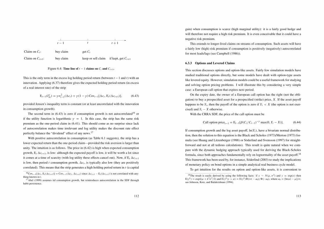
t − 1 t t + 1

Claim on Ct : buy claim get Ct

Claim on Ct+1: buy claim keep or sell claim if kept, get Ct+1

Figure 6.4: Time line of t − 1 claims on Ct and Ct+1.

This is the only term in the excess log holding period return (between t − 1 and t) with aninnovation. Applying (6.37) therefore gives the expected holding period return (in excessof a real interest rate) of the strip

Et−1(r eht) = γ σ 2

t−1(1ct)+ γ (1 − γ )Covt−1[1ct ,Et(1ct+1)], (6.43)

provided Jensen’s inequality term is constant (or at least uncorrelated with the innovationin consumption growth).

The second term in (6.43) is zero if consumption growth is not autocorrelated16 orif the utility function is logarithmic γ = 1. In this case, the strip has the same riskpremium as the one-period claim in (6.41). This should come as no surprise since lackof autocorrelation makes time irrelevant and log utility makes the discount rate effectperfectly balance the “dividend” effect of any news.17

With positive autocorrelation in consumption (as Table 6.1 suggests), the strip has alower expected return than the one-period claim—provided the risk aversion is larger thanunity. The intuition is as follows. The price in (6.42) is high when expected consumptiongrowth, Et 1ct+1, is low: although the expected payoff is low, it will be worth a lot sinceit comes at a time of scarcity (with log utility these effects cancel out). Now, if Et 1ct+1

is low, then period t consumption growth, 1ct , is typically also low (they are positivelycorrelated). This means that the strip generates a high holding period return in t (a capital

16Covt−1[1ct ,Et (1ct+1)] = Covt−1(1ct ,1ct+1) since 1ct+1 − Et (1ct+1) is not correlated with any-thing known in t .

17Abel (1999) assumes iid consumption growth, but reintroduces autocorrelation in the SDF throughhabit persistence.

112

gain) when consumption is scarce (high marginal utility): it is a fairly good hedge andwill therefore not require a high risk premium. It is even conceivable that it could have anegative risk premium.

This extends to longer-lived claims on streams of consumption. Such assets will havea fairly low (high) risk premium if consumption is positively (negatively) autocorrelatedfor most leads/lags (see Campbell (1986)).

6.3.3 Options and Levered Claims

This section discusses options and option-like assets. Fairly few simulation models havestudied traditional options directly, but some models have dealt with option-type assetslike levered equity. However, simulation models could be a useful framework for studyingand solving option pricing problems. I will illustrate this by considering a very simplecase: a European call option that expires next period.

On the expiry date, the owner of a European call option has the right (not the obli-gation) to buy a prespecified asset for a prespecified (strike) price, X . If the asset payoffhappens to be Yt , then the payoff of the option is zero if Yt < X (the option is not exer-cised) and Yt − X otherwise.

With the CRRA SDF, the price of the call option must be

Call option pricet−1 = Et−1[β(Ct/Ct−1)−γ max(0, Yt − X)]. (6.44)

If consumption growth and the log asset payoff, ln(Yt), have a bivariate normal distribu-tion, then the solution to this equation is the Black and Scholes (1973)/Merton (1973) for-mula (see Huang and Litzenberger (1988) or Soderlind and Svensson (1997) for straight-forward and not at all tedious calculations). This result is quite natural when we com-pare with the dynamic hedging approach typically used for deriving the Black-Scholesformula, since both approaches fundamentally rely on lognormality of the asset payoff.18

This framework has been used by, for instance, Soderlind (2003) to study the implicationsof monetary policy on bond options in a simple analytical real business cycle model.

To get intuition for the results on option and option-like assets, it is convenient to

18The result is easily derived by using the following facts: if x ∼ N (µ, σ 2) and y = exp(x) thenE(yk) = exp(kµ + k2σ 2/2) and E(yk

|y > a) = E(yk)8(rσ − a0)/8(−a0), where a0 = [ln(a) − µ]/σ ;see Johnson, Kotz, and Balakrishnan (1994).

113

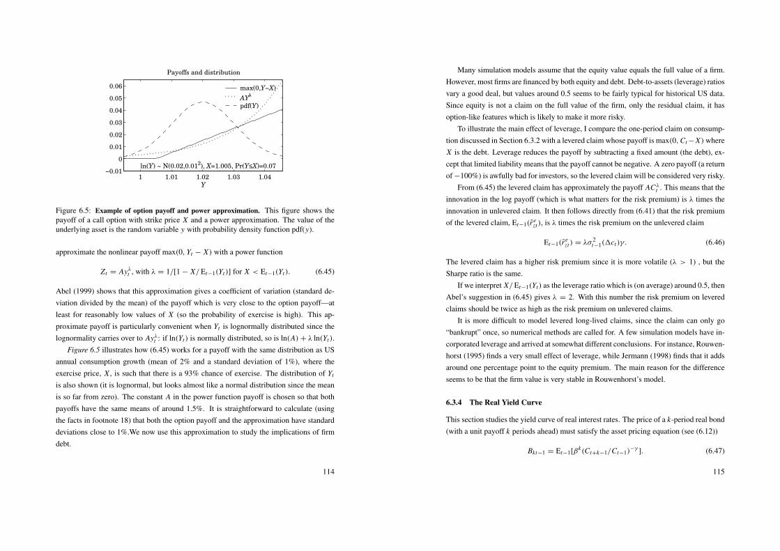
1 1.01 1.02 1.03 1.04−0.01

0

0.01

0.02

0.03

0.04

0.05

0.06

Payoffs and distribution

Y

ln(Y) ~ N(0.02,0.012), X=1.005, Pr(Y≤X)=0.07

max(0,Y−X)

AYλ

pdf(Y)

Figure 6.5: Example of option payoff and power approximation. This figure shows thepayoff of a call option with strike price X and a power approximation. The value of theunderlying asset is the random variable y with probability density function pdf(y).

approximate the nonlinear payoff max(0, Yt − X) with a power function

Z t = Ayλt , with λ = 1/[1 − X/Et−1(Yt)] for X < Et−1(Yt). (6.45)

Abel (1999) shows that this approximation gives a coefficient of variation (standard de-viation divided by the mean) of the payoff which is very close to the option payoff—atleast for reasonably low values of X (so the probability of exercise is high). This ap-proximate payoff is particularly convenient when Yt is lognormally distributed since thelognormality carries over to Ayλt : if ln(Yt) is normally distributed, so is ln(A)+ λ ln(Yt).

Figure 6.5 illustrates how (6.45) works for a payoff with the same distribution as USannual consumption growth (mean of 2% and a standard deviation of 1%), where theexercise price, X , is such that there is a 93% chance of exercise. The distribution of Yt

is also shown (it is lognormal, but looks almost like a normal distribution since the meanis so far from zero). The constant A in the power function payoff is chosen so that bothpayoffs have the same means of around 1.5%. It is straightforward to calculate (usingthe facts in footnote 18) that both the option payoff and the approximation have standarddeviations close to 1%.We now use this approximation to study the implications of firmdebt.

114

Many simulation models assume that the equity value equals the full value of a firm.However, most firms are financed by both equity and debt. Debt-to-assets (leverage) ratiosvary a good deal, but values around 0.5 seems to be fairly typical for historical US data.Since equity is not a claim on the full value of the firm, only the residual claim, it hasoption-like features which is likely to make it more risky.

To illustrate the main effect of leverage, I compare the one-period claim on consump-tion discussed in Section 6.3.2 with a levered claim whose payoff is max(0,Ct −X)whereX is the debt. Leverage reduces the payoff by subtracting a fixed amount (the debt), ex-cept that limited liability means that the payoff cannot be negative. A zero payoff (a returnof −100%) is awfully bad for investors, so the levered claim will be considered very risky.

From (6.45) the levered claim has approximately the payoff ACλt . This means that the

innovation in the log payoff (which is what matters for the risk premium) is λ times theinnovation in unlevered claim. It then follows directly from (6.41) that the risk premiumof the levered claim, Et−1(r e

zt), is λ times the risk premium on the unlevered claim

Et−1(r ezt) = λσ 2

t−1(1ct)γ. (6.46)

The levered claim has a higher risk premium since it is more volatile (λ > 1) , but theSharpe ratio is the same.

If we interpret X/Et−1(Yt) as the leverage ratio which is (on average) around 0.5, thenAbel’s suggestion in (6.45) gives λ = 2. With this number the risk premium on leveredclaims should be twice as high as the risk premium on unlevered claims.

It is more difficult to model levered long-lived claims, since the claim can only go“bankrupt” once, so numerical methods are called for. A few simulation models have in-corporated leverage and arrived at somewhat different conclusions. For instance, Rouwen-horst (1995) finds a very small effect of leverage, while Jermann (1998) finds that it addsaround one percentage point to the equity premium. The main reason for the differenceseems to be that the firm value is very stable in Rouwenhorst’s model.

6.3.4 The Real Yield Curve

This section studies the yield curve of real interest rates. The price of a k-period real bond(with a unit payoff k periods ahead) must satisfy the asset pricing equation (see (6.12))

Bkt−1 = Et−1[βk(Ct+k−1/Ct−1)

−γ]. (6.47)

115

-

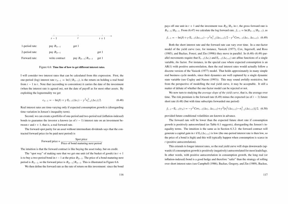
t − 1 t t + 1

1-period rate: pay B1t−1 get 1

2-period rate: pay B2t−1 get 1

Forward rate: write contract pay B2t−1/B1t−1 get 1

Figure 6.6: Time line of how to get different interest rates.

I will consider two interest rates that can be calculated from this expression. First, theone-period (log) interest rate r1t−1 = ln(1/B1t−1), is the return on holding a real bondfrom t − 1 to t . Note that (according to convention) it carries the date of the investment(when the interest rate is agreed on), not the date of payoff as for most other assets. Byexploiting the lognormality we get

r1t−1 = − ln(β)+ γ Et−1(1ct)− γ 2σ 2t−1(1ct)/2. (6.48)

Real interest rates are time-varying only if expected consumption growth is (disregardingtime-variation in Jensen’s inequality term).

Second, we can create a portfolio of one-period and two-period real (inflation-indexed)bonds to guarantee the investor a known (as of t − 1) interest rate on an investment be-tween t and t + 1, that is, a real forward rate.

The forward-spot parity for an asset without intermediate dividends says that the con-tracted forward price (to be paid next period) is

Forward price =Spot price

Price of bond maturing next period.

The intuition is that the forward contract is like buying the asset today, but on credit.The “spot way” of making sure that we get one unit (of the basket of goods) in t + 1

is to buy a two-period bond in t − 1 at the price B2t−1. The price of a bond maturing nextperiod is B1t−1, so the forward price is B2t−1/B1t−1. This is illustrated in Figure 6.6.

We then define the forward rate as the rate of return on this investment: since the bond

116

pays off one unit in t + 1 and the investment was B2t/B1t in t , the gross forward rate isB1t−1/B2t−1. From (6.47) we calculate the log forward rate, ft−1 = ln(B1t−1/B2t−1), as

ft−1 = − ln(β)+γ Et−1(1ct+1)−γ2σ 2

t−1(1ct+1)/2−γ 2 Covt−1(1ct ,1ct+1). (6.49)

Both the short interest rate and the forward rate can vary over time. In a one-factormodel of the yield curve (see, for instance, Vasicek (1977), Cox, Ingersoll, and Ross(1985), and Backus, Foresi, and Zin (1998)) they move in parallel. In (6.48)–(6.49) par-allel movements require that Et−1(1ct) and Et−1(1ct+1) are affine functions of a singlevariable, the factor. For instance, in the special case where expected consumption is anAR(1) with positive autocorrelation, then the real interest rates would actually follow adiscrete version of the Vasicek (1977) model. That holds approximately in many simplereal business cycle models, since their dynamics are well captured by a single dynamicstate variable (see Cogley and Nason (1993)). This may sound awfully restrictive, butfrom the perspective of modelling the real yield curve, it may be acceptable. It still amatter of debate of whether the one-factor model can be rejected or not.

We now turn to studying the average slope of the yield curve, that is, the average overtime. The risk premium is the forward rate (6.49) minus the expected (as of t − 1) futureshort rate (6.48) (but with time subscripts forwarded one period)

ft−1−Et−1(r1t) = −γ 2 Covt−1(1ct ,1ct+1)+γ2[σ 2

t (1ct+1)−σ2t−1(1ct+1)]/2, (6.50)

provided future conditional volatilities are known in advance.The forward rate will be lower than the expected future short rate if consumption

growth is positively autocorrelated (as Table 6.1 suggests), disregarding the Jensen’s in-equality terms. The intuition is the same as in Section 6.3.2: the forward contract willgenerate a capital gain in t if Et(1ct+1) is low (the one-period interest rate is then low, sothe price of a bond is high) and this will typically happen when consumption is scarce int (positive autocorrelation).

This extends to longer interest rates, so the real yield curve will slope downwards (up-wards) if consumption growth is positively (negatively) autocorrelated for most leads/lags.In other words, with positive autocorrelation in consumption growth, the long real (orinflation-indexed) bond is a good hedge and therefore “safer” than the strategy of rollingover short interest rates (see Campbell (1986), Backus, Gregory, and Zin (1989), Backus,

117

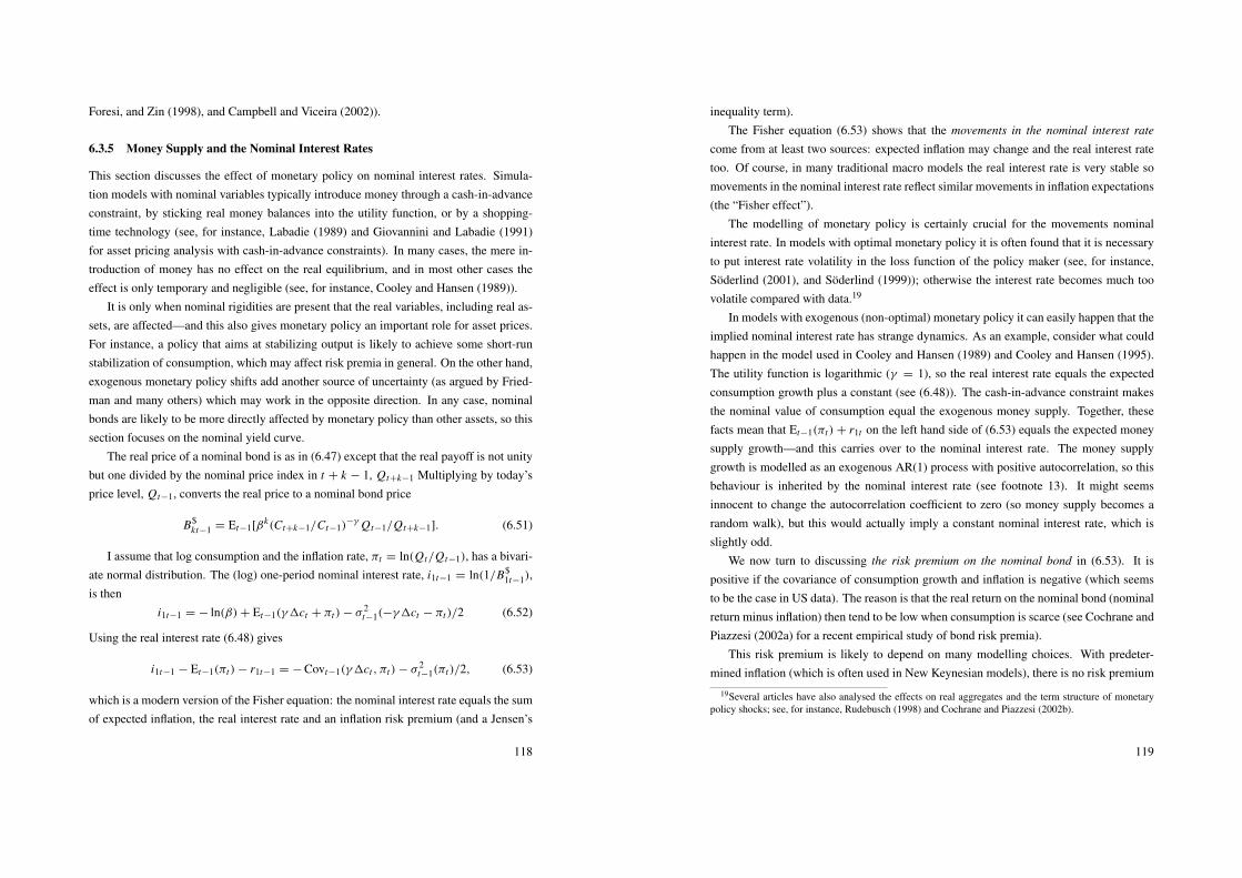
Foresi, and Zin (1998), and Campbell and Viceira (2002)).

6.3.5 Money Supply and the Nominal Interest Rates

This section discusses the effect of monetary policy on nominal interest rates. Simula-tion models with nominal variables typically introduce money through a cash-in-advanceconstraint, by sticking real money balances into the utility function, or by a shopping-time technology (see, for instance, Labadie (1989) and Giovannini and Labadie (1991)for asset pricing analysis with cash-in-advance constraints). In many cases, the mere in-troduction of money has no effect on the real equilibrium, and in most other cases theeffect is only temporary and negligible (see, for instance, Cooley and Hansen (1989)).

It is only when nominal rigidities are present that the real variables, including real as-sets, are affected—and this also gives monetary policy an important role for asset prices.For instance, a policy that aims at stabilizing output is likely to achieve some short-runstabilization of consumption, which may affect risk premia in general. On the other hand,exogenous monetary policy shifts add another source of uncertainty (as argued by Fried-man and many others) which may work in the opposite direction. In any case, nominalbonds are likely to be more directly affected by monetary policy than other assets, so thissection focuses on the nominal yield curve.

The real price of a nominal bond is as in (6.47) except that the real payoff is not unitybut one divided by the nominal price index in t + k − 1, Qt+k−1 Multiplying by today’sprice level, Qt−1, converts the real price to a nominal bond price

B$kt−1 = Et−1[β

k(Ct+k−1/Ct−1)−γ Qt−1/Qt+k−1]. (6.51)

I assume that log consumption and the inflation rate, πt = ln(Qt/Qt−1), has a bivari-ate normal distribution. The (log) one-period nominal interest rate, i1t−1 = ln(1/B$

1t−1),is then

i1t−1 = − ln(β)+ Et−1(γ1ct + πt)− σ 2t−1(−γ1ct − πt)/2 (6.52)

Using the real interest rate (6.48) gives

i1t−1 − Et−1(πt)− r1t−1 = − Covt−1(γ1ct , πt)− σ 2t−1(πt)/2, (6.53)

which is a modern version of the Fisher equation: the nominal interest rate equals the sumof expected inflation, the real interest rate and an inflation risk premium (and a Jensen’s

118

inequality term).The Fisher equation (6.53) shows that the movements in the nominal interest rate

come from at least two sources: expected inflation may change and the real interest ratetoo. Of course, in many traditional macro models the real interest rate is very stable somovements in the nominal interest rate reflect similar movements in inflation expectations(the “Fisher effect”).

The modelling of monetary policy is certainly crucial for the movements nominalinterest rate. In models with optimal monetary policy it is often found that it is necessaryto put interest rate volatility in the loss function of the policy maker (see, for instance,Soderlind (2001), and Soderlind (1999)); otherwise the interest rate becomes much toovolatile compared with data.19

In models with exogenous (non-optimal) monetary policy it can easily happen that theimplied nominal interest rate has strange dynamics. As an example, consider what couldhappen in the model used in Cooley and Hansen (1989) and Cooley and Hansen (1995).The utility function is logarithmic (γ = 1), so the real interest rate equals the expectedconsumption growth plus a constant (see (6.48)). The cash-in-advance constraint makesthe nominal value of consumption equal the exogenous money supply. Together, thesefacts mean that Et−1(πt) + r1t on the left hand side of (6.53) equals the expected moneysupply growth—and this carries over to the nominal interest rate. The money supplygrowth is modelled as an exogenous AR(1) process with positive autocorrelation, so thisbehaviour is inherited by the nominal interest rate (see footnote 13). It might seemsinnocent to change the autocorrelation coefficient to zero (so money supply becomes arandom walk), but this would actually imply a constant nominal interest rate, which isslightly odd.

We now turn to discussing the risk premium on the nominal bond in (6.53). It ispositive if the covariance of consumption growth and inflation is negative (which seemsto be the case in US data). The reason is that the real return on the nominal bond (nominalreturn minus inflation) then tend to be low when consumption is scarce (see Cochrane andPiazzesi (2002a) for a recent empirical study of bond risk premia).

This risk premium is likely to depend on many modelling choices. With predeter-mined inflation (which is often used in New Keynesian models), there is no risk premium

19Several articles have also analysed the effects on real aggregates and the term structure of monetarypolicy shocks; see, for instance, Rudebusch (1998) and Cochrane and Piazzesi (2002b).

119

at all. Monetary policy is also likely to affect the risk premium. For instance, in newKeynesian models with some kind of Phillips curve (sticky, but forward looking, pricesetting, see, for instance, Clarida, Galı, and Gertler (1999)) output (consumption) andinflation move in the same direction if demand shocks (random movements in the timepreference rate) dominate, but in opposite directions if supply shocks (random move-ments in productivity or factor input prices) dominate. If the monetary policy objectiveis to minimize some linear combination of variances of output and inflation without anyregard to interest rate volatility, then it is well known that monetary policy should neu-tralize all demand shocks but only some of the supply shocks. This will tend to make riskpremium positive.

6.3.6 Time-Variation in Risk Premia

This section briefly discusses how a simulation model can generate time-variation in riskpremia. Recall from (6.22) that the Sharpe ratio in the CRRA model is

Et−1(Ret ) = Covt−1(Re

t ,1ct) (6.54)

= ρt−1(Ret ,1ct)× σt−1(1ct)× σt−1(Re

t )γ. (6.55)

To get movements in risk premia in the consumption-based model, the conditional co-variance of the excess return and consumption growth must be changing over time. Fewsimulation models generate this because of a combination of two features: the shocks aretypically homoskedastic and the dynamics is close to log-linear (so consumption growthand log returns are linear transformations of the shocks). The result is that all expectedasset returns will (almost) move in parallel with the expected riskfree rate.

This can be changed by introducing heteroskedastic shocks. However, from (6.55) wesee that time-variation in the volatility of returns only (with constant correlations) willmake expected return move, but not Sharpe ratios. Similarly, time-variation in consump-tion volatility leads to proportional increases of the expected return and Sharpe ratios forall assets.

6.3.7 The Value of a Firm: Labour Contracts and Installation Costs

This section discusses how non-Walrasian labour contracts and installation costs (for newcapital) affects the equity value. We put aside the issue of how the total value of a firm is

120

split between equity holders and creditors in order to focus on the value of their combinedstake. The traditional way of modelling a firm is to assume that it hires labour and financesinvestment through retained earnings (no debt). Any extra cash flow is distributed asdividends

Dt = Yt − wt L t − It , (6.56)

where Yt is output, wt the real wage rate, L t labour input, and It investment costs. In real-ity most firms seem to smooth dividends, so Dt should probably not be directly comparedwith dividends, but with cash flows or earnings. Typically, the number of shares is keptconstant and normalized to unity.

Most simulation models have a Cobb-Douglas production function Y = Z t K αt L1−α

t ,where Z t is the technology level, Kt capital stock, and L t is labour input. The first ordercondition for hiring labour is that the real wage rate equals the marginal product of labour,wt = (1 − α)Y/L t . This does not require a competitive labour market, only that the firmcan hire freely at the going wage rate (“right to manage”). With this assumption, we canwrite (6.56) as

Dt = αYt − It . (6.57)

As side remark, we note that a high capital share, α, makes dividends fairly similar toconsumption (the aggregate resource constraint is Yt = It +Ct ), so the consumption claimmight be a good proxy for equity in that (admittedly unrealistic) case. In other cases, thedynamics of dividends and consumption can be quite different but many models still seemto generate too stable dividends (see, for instance, Rouwenhorst (1995)). The basic reasonis that neither aggregate output nor aggregate investments are nearly as volatile as cashflows and earnings on listed firms.

One possibility of making the cash flow process more realistic is to allow for labourhoarding (or other types of labour contracts that stabilizes the wage bill) and variationin the capacity utilization rate. Labour hoarding would make the wage bill relativelyconstant, rather than proportional to output as above. As a consequence, the cash flowwould fluctuate more in response to movements in output. For instance, Danthine andDonaldson (2002) study the implications different types of labour contracts in a settingwhere the priority status of wage claims creates an operational leverage (see also Section6.3.3 for a discussion of leverage)—and find that this can create a sizeable risk premium.

It has also been suggested that investments should be subject to installation costs.

121

Equations (6.56) and (6.57) are still true (It is the investment cost, not the gross additionof capital), but the behaviour of output, investment, and consumption will change. In par-ticular, installation costs will make consumption more volatile since it makes consump-tion smoothing more costly (see, for instance, Jermann (1998) and Lettau (2000)). Forinstance, when it is prohibitively expensive to change the investment from some steadystate level, then there is no consumption smoothing. Also, cash flows in (6.57) will reactstronger to output than before, since investments will no longer move in the same direc-tion as output. Both these effects tend to increase the equity premium, although it shouldbe admitted that increased consumption volatility is something of a cheat since that isnot a free parameter. (It could also be noted that installation costs leads to movements inTobin’s q, which seems to be a salient feature of data.)

6.3.8 Adding Assets to a Model

This section discusses if we really need fully-fledged equilibrium models to analyse thepricing of assets. The asset price in (6.12) is Pt = Et [6

∞

s=1βs(Ct+s/Ct)

−γ Dt+s], whereDt+s is the “dividend” in t + s. On a mechanical level, we probably need some kind ofmodel to calculate the the joint distribution of Ct+s and Dt+s . For instance, to price is aone-period real bond (Dt+1 = 1 and Dt+s = 0 for s > 1) we need the model to calculateEt [β(Ct+1/Ct)

−γ].

However, if the introduction of the asset does not change the process of consumption,then there is no need for explicitly including the asset (in the budget restriction and invest-ment opportunity set of investors) when solving the model. This is the case when we areusing a model with complete markets (the stochastic discount factor is unique in this case;see the references in footnote 2). In such a model, we could always analyse the pricing ofany asset, for instance, some really exotic derivative, without solving the model anew.

We are in a completely different situation when we introduce non-redundant assets,that is, when we add a non-trivial asset to a model with incomplete markets. In that casewe have solve the model with all the assets explicitly incorporated since their existence islikely to affect the equilibrium consumption process. Of course, specifying an exogenousprocess for nonstorable endowments circumvents the problem, which may explain whythat approach is so popular.

Most (simulation based) studies of imperfect markets have concentrated on idiosyn-cratic income risk that cannot be insured and on borrowing constraints/transaction costs.

122

The key findings and references are given in Section 6.2.6. Other studies have developedsolution methods and analysed a different set of incomplete markets. For instance, Juddand Guu (2001) show that introducing an option on the stock market can lower the equitypremium considerably (see also Den Haan (1996) and Marcet and Singleton (1999) forsolution methods and some examples).

6.4 Summary

The first part of this chapter studies the consumption-based asset pricing model with con-stant relative risk aversion (CRRA) by comparing the model predictions to the moments(means, variances, and correlations) of US consumption growth and returns on broad assetclasses.

It is shown that the smooth consumption growth rate observed in the US makes it hardto explain the equity premium, unless the risk aversion is very high (this is the equitypremium puzzle discussed in Mehra and Prescott (1985)). However, a very high riskaversion seems somewhat implausible and it creates other problems. In particular, a largerisk aversion coefficient makes it hard to reconcile average consumption growth with theaverage return on riskfree assets (this is the riskfree rate puzzle discussed in Weil (1989))and the low volatility of real interest rates (or approximations of it).

One reaction to these problems is to say that the consumption-based model may failto explain the magnitude of the risk premium, but that it at least can be used to understandqualitative differences in average return. For instance, the model correctly predicts higherreturns on equity than on bonds. One of main issues in the first part of the chapter is howfar that argument can be extended. Data on Sharpe ratios for different portfolios sorted onindustry, dividend-price ratio, size, book-to-market, and geographical location show thatthe consumption-based model is unable to explain the cross-sectional variation of Sharperatios. The basic problems seems to be that there is a lot of dispersion in Sharpe ratios, butmost portfolio returns are only weakly correlated with aggregate consumption growth. Itis also shown that the consumption-based model fails badly in explaining time-variationof equity premia. Although the covariance of consumption and equity returns changesover time, it does so in completely the wrong way compared with excess returns.

All these problems have spurred interest in developing the consumption-based modelby changing the utility function and/or introducing heterogenous agents. Several of these

123

suggestions (Epstein-Zin preferences, habit formation, and idiosyncratic risk) are anal-ysed at the end of the first part of the chapter. It is found that they are quite successful insolving some of the problems, but that several remain unsolved. In particular, none of thesuggestions make much headway with the cross-sectional variation of Sharpe ration.

The second part of the chapter is a theoretical analysis of the equilibrium relationbetween different asset returns and the consumption process. Simple pricing expressions(based on assumptions about lognormal returns and consumption growth) highlights thebasic mechanism of (otherwise) fairly complicated pricing problems. Among the results,we find the following.

First, a positive autocorrelation of consumption growth is likely to give low risk pre-mia on long-lived consumption claims and a negatively sloped real yield curve. Second,the properties of the Fisher equation and the risk premium on nominal bonds depend cru-cially on monetary policy. For instance, shocks to aggregate demand typically move con-sumption and inflation in the same direction, so the standard recipe for monetary policyis cushion all such shocks. However, this is likely to increase the inflation risk premiumsince it makes inflation and consumption more negatively correlated (so the real return onthe nominal bond tend to be low when consumption is scarce). Third, options and leveredclaims will typically have higher risk premia than the underlying asset/unlevered claimbecause their returns are more volatile.

Simulation models have made fine contributions to the analysis of asset pricing. Inparticular, they have taught us a great deal about how the properties of the consumption-based asset model with constant relative risk aversion (CRRA). However, it is clear thatthe CRRA model has serious problems on many accounts and much of the current re-search is trying models with different utility functions and/or different measures of con-sumption. We still know too little about the properties of these new models, for instance,what side effects they have. This is likely to be the next area where simulation modelsmake valuable contributions to the asset pricing literature.

A Data Appendix

The nominal US stock returns are from the website of French (2001). These monthlyreturns are converted to quarterly returns by multiplying the monthly gross returns, forinstance, the gross returns for January, February, and March are multiplied to generate

124

a quarterly gross return. The portfolios are formed from NYSE, AMEX, and NASDAQfirms. The aggregate stock market return is a value weighted return of all available re-turns. The (equally-weighted) portfolios based on industry, size, dividend/price, or book-to-market are from the same data set, but with the firms sorted on the respective charac-teristic. The ten industry portfolios are for consumer nondurable, consumer durables, oil,chemicals, manufacturing, telecom, utilities, wholesale and retail, financial services, andother. The ten size portfolios are for deciles of firm market values; the D/P portfolios arefor deciles of dividend/price; and the B/M portfolios are for deciles of book value/marketvalues.

The dividend-price ratio for S&P500 is from Shiller (2000).The nominal return on long US government bonds is from Ibbotson Associates.The international stock and long government bond returns are from Ibbotson Asso-

ciates, but come originally from Morgan Stanley and IMF respectively. The internationaldata is for France, Germany, Japan, and United Kingdom, and has been converted into USdollar returns.

Real returns are calculated by dividing the nominal gross return by the gross inflationrate over the same period. Inflation is calculated from the seasonally adjusted CPI for allurban consumers (available at http://www.stls.frb.org/fred/).

Quarterly growth of real consumption per capita of nondurables and services is calcu-lated from the seasonally adjusted number in NIPA Table 8.7 (available at http://www.bea.doc.gov/bea/dn1.htm). The growth rate is calculated as a weighted average of the growthrate of nondurables and the growth rate of services (chained 1996 dollars), where the(time-varying) weight is the relative (current dollar) size of nondurables in relation toservices.

The annualized k-quarter excess return used in the discussion of stock returns pre-dictability are calculated as Re

t (k) = (Rt Rt−1...Rt−k+1)4/k

− (R f t R f t−1...R f t−k+1)4/k ,

where Rt is the quarterly gross return of the aggregate US stock market (see above) andR f t is the quarterly gross return on a short T-bill.

B Econometrics Appendix

The tests in Table 6.1 are based on t-tests from a GMM estimation and the delta method.Testing of the mean, standard deviation, and Sharpe ratio is done in the following

125

way. First, moment conditions for the mean (µ) and second moment (χ ) of the randomvariable xt are defined as

∑Tt=1mt(β)/T = 02×1 where mt =

[xt − µ

x2t − χ

]and β =

[µ

χ

].

GMM estimation is trivial and the estimator is asymptotically normally distributed aroundthe true value β0 as

√T (β − β0)

d→ N (02×1, S0),

where S0 is the variance-covariance matrix of6Tt=1mt(β0)/

√T , which can be consistently

estimated by using the point estimate of β instead of β0 and then applying the Newey andWest (1987) estimator. Second, the standard deviation and Sharpe ratio are calculated asfunctions of β[

σ(x)

E(x)/σ (x)

]= g(β) =

[(χ − µ2)1/2

µ

(χ−µ2)1/2

], so

∂g(χ, µ)∂β ′

=

[−µ

(χ−µ2)1/21

2(χ−µ2)1/2

χ

(χ−µ2)3/2−µ

2(χ−µ2)3/2

].

From the delta method we then have

√T [g(β)− g(β0)]

d→ N

(0,∂g (β0)

∂β′

S0∂g (β0)

′

∂β

),

which is used to construct asymptotic t-tests.A similar approach is used for testing the correlation of xt and yt , ρ(xt , yt). For

expositional simplicity, assume that both variables have zero means. The variances andthe covariance can then be estimated by the moment conditions

∑Tt=1mt(β)/T = 03×1 where mt =

x2t − σxx

y2t − σyy

xt yt − σxy

and β =

σxx

σyy

σxy

.The covariance matrix of these estimators is estimated as before. The correlation is asimple function of these parameters

ρ(x, y) = g(β) =σxy

σ1/2xx σ

1/2yy

, so∂g(χ, µ)∂β ′

=

[−

12

σxy

σ3/2xx σ

1/2yy

−12

σxy

σ1/2xx σ

3/2yy

1σ

1/2xx σ

1/2yy

].

The delta method formula (see above) is the applied to this case as well.

126

Bibliography

Abel, A. B., 1999, “Risk Premia and Term Premia in General Equilibrium,” Journal of

Monetary Economics, 43, 3–33.

Altug, S., and P. Labadie, 1994, Dynamic Choice and Asset Markets, Academic Press.

Backus, D., S. Foresi, and S. Zin, 1998, “Arbitrage opportunities in arbitrage-free modelsof bond pricing,” Journal of Business and Economic Statistics, 16, 13–26.

Backus, D., A. Gregory, and S. Zin, 1989, “Risk Premiums in the Term Structure; Evi-dence from Artificial Economies,” Journal of Monetary Economics, 24, 371–399.

Bansal, R., and C. Lundblad, 2002, “Market Efficiency, Fundamental Values, and theSize of the Risk Premium in Global Equity Markets,” Journal of Econometrics, 109,195–237.

Bidarkota, P. V., and J. H. McCulloch, 2003, “Consumption Asset Pricing with StableShocks - Exploring a Solution and Its Implications for Mean Equity Returns,” Journal

of Economic Dynamics and Control, 27, 399–421.

Black, F., and M. Scholes, 1973, “The Pricing of Options and Corporate Liabilities,”Journal of Political Economy, 81, 637–659.

Bossaert, P., 2002, The Paradox of Asset Pricing, Princeton University Press.

Breeden, D. T., 1979, “An Intertemporal Asset Pricing Model with Stochastic Consump-tion and Investment Opportunities,” Journal of Financial Economics, 7, 265–96.

Campbell, J. Y., 1986, “Bond and Stock Returns in a Simple Exchange Model,” Quarterly

Journal of Economics, 101, 785–804.

Campbell, J. Y., 1993, “Intertemporal Asset Pricing without Consumption Data,” Ameri-

can Economic Review, 83, 487–512.

Campbell, J. Y., 2001, “Consumption-Based Asset Pricing,” in George Constantinides,Milton Harris, and Rene Stultz (ed.), Handbook of the Economics of Finance, North-Holland, Amsterdam.

127

Campbell, J. Y., and J. H. Cochrane, 1999, “By Force of Habit: A Consumption-BasedExplanation of Aggregate Stock Market Behavior,” Journal of Political Economy, 107,205–251.

Campbell, J. Y., A. W. Lo, and A. C. MacKinlay, 1997, The Econometrics of Financial

Markets, Princeton University Press, Princeton, New Jersey.

Campbell, J. Y., and L. M. Viceira, 2002, Strategic Asset Allocation: Portfolio Choice of

Long-Term Investors, Oxford University Press.

Clarida, R., J. Galı, and M. Gertler, 1999, “The Science of Monetary Policy: A NewKeynesian Perspective,” Journal of Economic Literature, 37, 1661–1707.

Cochrane, J. H., 2001, Asset Pricing, Princeton University Press, Princeton, New Jersey.

Cochrane, J. H., and M. Piazzesi, 2002a, “Bond Risk Premia,” mimeo, University ofChicago.

Cochrane, J. H., and M. Piazzesi, 2002b, “The Fed and Interest Rates—a High-FrequencyIdentification,” AER Papers and Proceedings, 92, 90–95.

Cogley, T., 1998, “Idiosyncratic Risk and Equity Premium: Evidence from the ConsumerExpenditure Survey,” mimeo, Federal Reserve Bankl of San Francisco.

Cogley, T., and J. M. Nason, 1993, “Impulse Dynamics and Propagation Mechanisms inReal Busines Cycle Model,” Economics Letters, 43, 77–81.

Constantinides, G. M., and D. Duffie, 1996, “Asset Pricing with Heterogeneous Con-sumers,” The Journal of Political Economy, 104, 219–240.

Cooley, T. F., and G. D. Hansen, 1989, “The Inflation Tax in a Real Business CycleModel,” The American Economic Review, 79, 733–748.

Cooley, T. F., and G. D. Hansen, 1995, “Money and the Business Cycle,” in Thomas F.Cooley (ed.), Frontiers of Business Cycle Research, Princeton University Press, Prince-ton, New Jersey.

Cox, J. C., J. E. Ingersoll, and S. A. Ross, 1985, “A Theory of the Term Structure ofInterest Rates,” Econometrica, 53, 385–407.

128

Danthine, J.-P., and J. B. Donaldson, 2002, “Labour Relations and Asset Returns,” Review

of Economic Studies, 69, 41–64.

Den Haan, W. J., 1996, “Heterogeneity, Aggregate Uncertainty, and the Short-Term In-terest Rate,” Journal of Business and Economic Statistics, 14, 399–411.

Den Haan, W. J., 2001, “The Importance of the Number of Different Agents in a Heteroge-nous Asset-Pricing Model,” Journal of Economic Dynamics and Control, 25, 721–746.

Epstein, L. G., and S. E. Zin, 1989a, “Substitution, Risk Aversion, and the TemporalBehavior of Asset Returns: A Theoretical Framework,” Econometrica, 57, 937–969.

Epstein, L. G., and S. E. Zin, 1989b, “Substitution, Risk Aversion, and the TemporalBehavior of Asset Returns: An Empirical Analysis,” Journal of Political Economy, 99,263–286.

Fama, E. F., and K. R. French, 1988a, “Dividend Yields and Expected Stock Returns,”Journal of Financial Economics, 22, 3–25.

Fama, E. F., and K. R. French, 1988b, “Permanent and Temporary Components of StockPrices,” Journal of Political Economy, 96, 246–273.

Fama, E. F., and K. R. French, 1993, “Common Risk Factors in the Returns on Stocksand Bonds,” Journal of Financial Economics, 33, 3–56.

Ferson, W. E., 1995, “Theory and Empirical Testing of Asset Pricing Models,” inRobert A. Jarrow, Vojislav Maksimovic, and William T. Ziemba (ed.), Handbooks in

Operations Research and Management Science . pp. 145–200, North-Holland.

French, K. R., 2001, “U.S. Research Returns Data,” http://mba.tuck.dartmouth.edu/pages/faculty/ken.french/.

Giovannini, A., and P. Labadie, 1991, “Asset Prices and Interest Rates in Cash-in-AdvanceModels,” Journal of Political Economy, 99, 1215–1251.

Hansen, L. P., and R. Jagannathan, 1991, “Implications of Security Market Data for Mod-els of Dynamic Economies,” Journal of Political Economy, 99, 225–262.

129

Hansen, L. P., and S. F. Richard, 1987, “The Role of Conditioning Information in Deduc-ing Testable Restrictions Implied by Dynamic Asset Pricing Models,” Econometrica,55, 587–613.

Harrison, M. J., and D. M. Kreps, 1979, “Martingales and Arbitrage in Multiperiod Secu-rities Markets,” Journal of Economic Theory, 20, 381–408.

He, H., and D. M. Modest, 1995, “Market Frictions and Consumption-Based Asset Pric-ing,” Journal of Political Economy, 103, 94–117.

Heaton, J. C., and D. J. Lucas, 1996, “Evaluating the Effects of Incomplete Markets onRisk-Sharing and Asset Pricing,” Journal of Political Economy, 104, 443–487.

Hendershott, P. H., 1998, “Equilibrium Models in Real Estate Research: A Survey,” Jour-

nal of Real Estate Literature, 6, 13–25.

Huang, C.-F., and R. H. Litzenberger, 1988, Foundations for Financial Economics, Else-vier Science Publishing, New York.

Jermann, U. J., 1998, “Asset Pricing in Production Economies,” Journal of Monetary

Economics, 41, 257–275.

Johnson, N. L., S. Kotz, and N. Balakrishnan, 1994, Continuous Univariate Distributions,Wiley, New York, 2nd edn.

Judd, K. L., and S.-M. Guu, 2001, “Asymptotic Methods for Asset Market EquilibriumAnalysis,” Economic Theory, 18, 127–157.

Kollman, R., 2001, “The Exchange Rate in a Dynamic-Optimizing Business Cycle Modelwith Nominal Rigidities: A Quantitative Investigation,” Journal of International Eco-

nomics, 55, 243–262.

Labadie, P., 1989, “Stochastic Inflation and the Equity Premium,” Journal of Monetary

Economics, 24, 277–298.

LeRoy, S. F., and J. Werner, 2001, Principles of Financial Economics, Cambridge Uni-versity Press.

130

Lettau, M., 2000, “Inspecting the Mechanism: Closed-form Solutions for Asset Prices inReal Busines Cycle Models,” mimeo, Federal Reserve Bank of New York.

Lettau, M., 2002, “Idiosyncratic Risk and Volatility Bounds, or Can Models with Idiosyn-cratic Risk Solve the Equity Premium Puzzle,” Review of Economics and Statistics,forthcoming.

Lettau, M., and H. Uhlig, 2000, “Can Habit Formation Be Reconciled with BusinessCycle Facts,” Review of Economic Dynamics, 3, 79–99.

Lettau, M., and H. Uhlig, 2002, “Sharpe Ratios and Preferences: An Analytical Ap-proach,” Macroeconomic Dynamics, 6, 242–265.

Lintner, J., 1965, “The Valuation of Risky Assets and the Selection of Risky Investmentsin Stock Portfolios and Capital Budgets,” Review of Economics and Statistics, 47, 13–37.

Ljunqvist, L., and H. Uhlig, 2000, “Tax Policy and Aggregate Demand ManagementUnder Catching Up with the Joneses,” American Economic Review, 90, 356–366.

Lucas, R. E., 1978, “Asset Prices in an Exchange Economy,” Econometrica, 46, 1426–14.

Luttmer, E. G. J., 1996, “Asset pricing in Economies with Frictions,” Econometrica, 64,1439–1467.

Mankiw, G. N., 1986, “The Equity Premium and the Concentration of Aggregate Shocks,”Journal of Financial Economics, 17, 211–219.

Marcet, A., and K. J. Singleton, 1999, “Equilibrium Asset Prices and Savings of Het-erogeneous Agents in the Presence of Incomplete Markets and Portfolio Constraints,”Macroeconomic Dynamics, 3, 243–277.

Mehra, R., and E. Prescott, 1985, “The Equity Premium: A Puzzle,” Journal of Monetary

Economics, 15, 145–161.

Merton, R. C., 1973, “Rational Theory of Option Pricing,” Bell Journal of Economics and

Management Science, 4, 141–183.

Mossin, J., 1968, “Equilibrium in a Capital Asset Market,” Econometrica, 35, 768–783.

131

Newey, W. K., and K. D. West, 1987, “A Simple Positive Semi-Definite, Heteroskedastic-ity and Autocorrelation Consistent Covariance Matrix,” Econometrica, 55, 703–708.

Reffett, K., and F. Schorfheide, 2000, “Evaluating Asset Pricing Implications of DSGEModels,” mimeo, Arizona State University.

Ross, S. A., 1978, “A Simple Approach to the Valuation of Risky Streams,” Journal of

Business, 51, 453–475.

Rouwenhorst, K., 1995, “Asset Pricing Implications of Equilibrium Business Cycle Mod-els,” in Thomas F. Cooley (ed.), Frontiers of Business Cycle Research, Princeton Uni-versity Press, Princeton, New Jersey.

Rudebusch, G. D., 1998, “Do measures of monetary policy in a VAR make sense?,” In-

ternational Economic Review, 39, 907–931.

Salyer, K. D., 1998, “Crash States and the Equity Premium: Solving One Puzzle RaisesAnother,” Journal of Economic Dynamics and Control, 22, 955–965.

Sharpe, W. F., 1964, “Capital Asset Prices: A Theory of Market Equilibrium under Con-ditions of Risk,” Journal of Finance, 19, 425–442.

Shiller, R. J., 2000, Irrational Exuberance, Princeton University Press, data available athttp://www.econ.yale.edu/ shiller/data.htm.

Smith, P. N., and M. R. Wickens, 2002, “Asset Pricing with Observable Stochastic Dis-count Factors,” Discussion Paper No. 2002/03, University of York.

Soderlind, P., 1999, “Solution and Estimation of RE Macromodels with Optimal Policy,”European Economic Review, 43, 813–823.

Soderlind, P., 2001, “Monetary Policy and the Fisher Effect,” Journal of Policy Modeling,23, 491–495.

Soderlind, P., 2003, “Monetary Policy and Bond Option Pricing in an Analytical RBCModel,” WP 447, Stockholm School of Economics, Forthcoming in Journal of Eco-

nomics and Business.

132

Soderlind, P., and L. E. O. Svensson, 1997, “New Techniques to Extract Market Expecta-tions from Financial Instruments,” Journal of Monetary Economics, 40, 383–420.

Svensson, L. E. O., 1989, “Portfolio Choice with Non-expected Utility in ContinuousTime,” Economics Letters, 40, 313–317.

Telmer, C. I., 1993, “Asset Pricing Puzzles and Incomplete Markets,” Journal of Finance,48, 1803–1832.

Vasicek, O. A., 1977, “An Equilibrium Characterization of the Term Structure,” Journal

of Financial Economics, 5, 177–188.

Vayanos, D., 1998, “Transaction Costs and Asset Prices: A Dynamic Equilibrium Model,”Review of Financial Studies, 11, 1–58.

Weil, P., 1989, “The Equity Premium Puzzle and the Risk-Free Rate Puzzle,” Journal of

Monetary Economics, 24, 401–421.

Zimmermann, C., 1999, “International Business Cycles and Exchange Rates,” Review of

International Economics, 74, 682–698.

133

7 ARCH and GARCH

Reference: Campbell, Lo, and MacKinlay (1997) 12.2; Hamilton (1994) 21; Greene(2000) 18.5; Hentschel (1995); Franses and van Dijk (2000)

7.1 Test of ARCH Effects

Suppose we have estimated a model, and obtained the fitted residuals, ut for t = 1, . . . , T .Engle’s test of ARCH (autoregressive conditional heteroskedasticity) is perhaps the moststraightforward. It amounts to running the regression

u2t = a0 +

∑q

s=1ai u2

t−s + vt . (7.1)

Under the null hypothesis of no ARCH effects, all slope coefficients are zero and the R2

of the regression is zero. These overidentifying restrictions can be tested by noting that,under the null hypothesis, T R2

∼ χ2q .

It is straightforward to phrase Engle’s test in terms of GMM moment conditions. Wesimply use a first set of moment conditions to estimate the parameters of the regressionmodel, and then test if the following additional (ARCH related) moment conditions aresatisfied at those parameters

E

u2

t−1...

u2t−s

(u2t − a0) = 0s×1. (7.2)

An alternative test (see Harvey (1989) 259–260), is to apply a Box-Ljung test on u2t , to

see if the squared fitted residuals are autocorrelated. We just have to adjust the degrees offreedom in the asymptotic chi-square distribution by subtracting the number of parametersestimated in the regression equation.

These tests for ARCH effects will typically capture GARCH (see below) effects aswell.

134

7.2 ARCH Models

A very simple ARCH(1) model is given by

yt = x ′

tb + ut , E(ut |xt) = 0 (7.3)

where xt is a k × 1 vector. The residual can be written

ut = vtσt with vt ∼ iid with Et−1 vt = 0 and Et−1 v2t = 1, (7.4)

and the conditional variance is generated by

σ 2t = α0 + α1u2

t−1, with α0 > 0 and 0 ≤ α1 < 1. (7.5)

(Note that my convention for the time subscript of the conditional variance is differentfrom that used in CLM. They use σ 2

t−1 to indicate the variance in t .)The non-negativity restrictions are needed in order to guarantee σ 2

t > 0. The upperbound α1 < 1 is needed in order to make the conditional variance stationary. To see this,use σ 2

t = Et−1 u2t to write (7.5) as

Et−1 u2t = α0 + α1u2

t−1, which implies (7.6)

E u2t = α0 + α1 E u2

t−1 or E u2t = α0/(1 − α1) (if α1 < 1). (7.7)

A value of α1 < 1 is clearly needed to make the difference equation stable and hence theunconditional variance finite.

It is clear that the unconditional distribution of ut is non-normal. Even if we assumethat vt is iid N (0, 1), we get that the conditional distribution of ut is N (0, σ 2

t ), so theunconditional distribution of ut is a mixture of normal distributions with different vari-ances. It can be shown that the result is a distribution which have fatter tails than a normaldistribution with the same variance (excess kurtosis).

Equation (7.6) shows how we can use information in t − 1 to forecast u2t . By leading

the time subscript one period we have

Et u2t+1 = α0 + α1u2

t , so

Et−1 u2t+1 = α0 + α1 Et−1 u2

t

= α0(1 + α1)+ α21u2

t−1, (7.8)

135

where we used (7.6) to substitute for Et−1 u2t . Similarly, for u2

t+2 we get from (7.8)

Et−1 u2t+2 = α0 + α1 Et−1 u2

t+1

= α0(1 + α1 + α21)+ α3

1u2t−1. (7.9)

The pattern for using information in t − 1 to forecast future volatility is now clear: itworks just like an AR(1). In fact, rearranging (7.8) and (7.9) shows that the forecastingequation can be written

Et−1 u2t+s −

α0

1 − α1= αs+1

1

(u2

t−1 −α0

1 − α1

), (7.10)

which describes the evolution of the Et−1 u2t+s around its unconditional mean as an AR(1).

The parameter α1 is therefore crucial for the persistence of shocks to volatility.Note that (7.3) is valid linear regression model (since the residual and regressors are

uncorrelated), so LS is consistent (and the most efficient linear estimator of b). Sincethe heteroskedasticity is not related to the regressors, the standard LS expression for thecovariance of the LS estimator of b should also continue to hold. However, there are moreefficient estimators than LS. Moreover, even if we are not too interested in efficiency, wemight be interested in the heteroskedasticity for its own sake. This suggests that we maywant to estimate the full model (7.3)–(7.5) by ML or GMM.

The most common way to estimate the model is to assume that vt ∼iid N (0, 1) andto set up the likelihood function. The log likelihood is easily found, since the model isconditionally Gaussian. It is

ln L = −T2

ln (2π)−12

T∑t=1

ln σ 2t −

12

T∑t=1

u2t

σ 2t

if vt is iid N (0, 1). (7.11)

By plugging in (7.3) for ut and (7.5) for σ 2t , the likelihood function is written in terms of

the data and model parameters. The likelihood function is then maximized with respectto the parameters. Note that we need a starting value of σ 2

1 = α0 + α1u20. The most

convenient (and common) way is maximize the likelihood function conditional on a y0

and x0. That is, we actually have a sample running from t = 0 to t = T , but observationt = 0 is only used to construct a starting value of σ 2

1 . The optimization should preferablyimpose the constraints in (7.5). The MLE is consistent.

136

Remark 33 (Coding the ARCH(1) ML estimation.) A straightforward way of coding

the estimation problem (7.3)–(7.5) and (7.11) is as follows. First, guess values of the

parameters b (a vector), and α0, and α1. The guess of b can be taken by LS estimation

of (7.3), and the guess of α0 and α1 from LS estimation of u2t = α0 + α1u2

t−1 + εt where

ut are the fitted residuals from the LS estimation of (7.3). Second, loop over the sample

(first t = 1, then t = 2, etc.) and estimate calculate ut from (7.3) and σ 2t from (7.5). Plug

in these numbers in (7.11) to find the likelihood value. Third, make better guesses of the

parameters and do the first two steps again. Repeat until the likelihood value converges

(at a maximum).

Remark 34 (Imposing parameter constraints on ARCH(1).) To impose the restrictions

in (7.5) when the previous remark is implemented, iterate over values of (b, α0, α1) and

let a0 = α20 and a1 = exp(a1)/[1 + exp(a1)]. This approach is particularly useful when a

numerical optimization routine is used.

If is often found that the fitted normalized residuals, ut/σt , still have too fat tailscompared with N (0, 1). Estimation using other likelihood functions, for instance, fora t-distribution, can then be used. Or the estimation can be interpreted as a quasi-ML(is typically consistent, but requires different calculation of the covariance matrix of theparameters).

Another possibility is to estimate the model by GMM using, for instance, the follow-ing the moment conditions (where σ 2

t is given by (7.5))

E

xtut

u2t − σ 2

t

u2t−1(u

2t − σ 2

t )

= 0(k+2)×1, where ut = yt − x ′

tb. (7.12)

It is straightforward to add more lags to (7.5). For instance, an ARCH(p) would be

σ 2t = α0 + α1u2

t−1 + . . .+ αpu2t−p. (7.13)

We then have to add more moment conditions to (7.12), but the form of the likelihoodfunction is the same except that we now need p starting values and that the upper boundaryconstraint should now be 6 p

j=1α j ≤ 1.

137

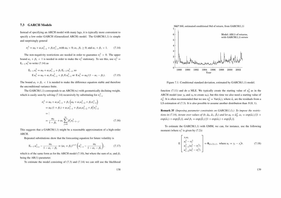
7.3 GARCH Models

Instead of specifying an ARCH model with many lags, it is typically more convenient tospecify a low-order GARCH (Generalized ARCH) model. The GARCH(1,1) is simpleand surprisingly general

σ 2t = α0 + α1u2

t−1 + β1σ2t−1,with α0 > 0; α1, β1 ≥ 0; and α1 + β1 < 1. (7.14)

The non-negativity restrictions are needed in order to guarantee σ 2t > 0. The upper

bound α1 + β1 < 1 is needed in order to make the σ 2t stationary. To see this, use σ 2

t =

Et−1 u2t to write (7.14) as

Et−1 u2t = α0 + α1u2

t−1 + β1 Et−2 u2t−1, so

E u2t = α0 + α1 E u2

t−1 + β1 E u2t−1 or E u2

t = α0/(1 − α1 − β1). (7.15)

The bound α1 + β1 < 1 is needed to make the difference equation stable and thereforethe unconditional variance finite.

The GARCH(1,1) corresponds to an ARCH(∞) with geometrically declining weight,which is easily seen by solving (7.14) recursively by substituting for σ 2

t−s

σ 2t = α0 + α1u2

t−1 + β1

(α0 + α1u2

t−2 + β1σ2t−2

)= α0 (1 + β1)+ α1u2

t−1 + β1α1u2t−2 + β2

1σ2t−2

=...

=α0

1 − β1+ α1

∞∑j=0

βj

1 u2t−1− j . (7.16)

This suggests that a GARCH(1,1) might be a reasonable approximation of a high-orderARCH.

Repeated substitutions show that the forecasting equation for future volatility is

Et−1 u2t+s −

α0

1 − α1 − β1= (α1 + β1)

s+1(

u2t−1 −

α0

1 − α1 − β1

), (7.17)

which is of the same form as for the ARCH model (7.10), but where the sum of α1 and β1

being the AR(1) parameter.To estimate the model consisting of (7.3) and (7.14) we can still use the likelihood

138

1988 1990 1992 1994 1996 1998 2000 20020

1

2

3

4

5

6

7S&P 500, estimated conditional Std of return, from GARCH(1,1)

Year

Model: AR(1) of returns,with GARCH(1,1) errors

Figure 7.1: Conditional standard deviation, estimated by GARCH(1,1) model.

function (7.11) and do a MLE. We typically create the starting value of u20 as in the

ARCH model (use y0 and x0 to create u0), but this time we also need a starting value ofσ 2

0 . It is often recommended that we use σ 20 = Var(ut), where ut are the residuals from a

LS estimation of (7.3). It is also possible to assume another distribution than N (0, 1).

Remark 35 (Imposing parameter constraints on GARCH(1,1).) To impose the restric-

tions in (7.14), iterate over values of (b, α0, α1, β1) and let a0 = α20 , a1 = exp(a1)/[1 +

exp(a1)+ exp(β1)], and β1 = exp(β1)/[1 + exp(a1)+ exp(β1)].

To estimate the GARCH(1,1) with GMM, we can, for instance, use the followingmoment (where σ 2

t is given by (7.2))

E

xtut

u2t − σ 2

t

u2t−1(u

2t − σ 2

t )

u2t−2(u

2t − σ 2

t )

= 0(k+3)×1, where ut = yt − x ′

tb. (7.18)

139

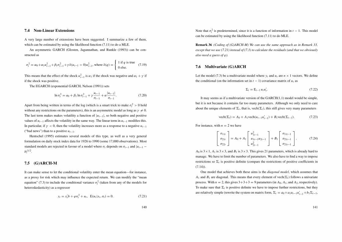
7.4 Non-Linear Extensions

A very large number of extensions have been suggested. I summarize a few of them,which can be estimated by using the likelihood function (7.11) to do a MLE.

An asymmetric GARCH (Glosten, Jagannathan, and Runkle (1993)) can be con-structed as

σ 2t = α0 +α1u2

t−1 +β1σ2t−1 +γ δ(ut−1 > 0)u2

t−1, where δ(q) =

{1 if q is true0 else.

(7.19)

This means that the effect of the shock u2t−1 is α1 if the shock was negative and α1 + γ if

if the shock was positive.The EGARCH (exponential GARCH, Nelson (1991)) sets

ln σ 2t = a0 + β1 ln σ 2

t−1 + γut−1

σt−1+ α

|ut−1|

σt−1. (7.20)

Apart from being written in terms of the log (which is a smart trick to make σ 2t > 0 hold

without any restrictions on the parameters), this is an asymmetric model as long as γ 6= 0.The last term makes makes volatility a function of |ut−1|, so both negative and positivevalues of ut−1 affects the volatility in the same way. The linear term in ut−1 modifies this.In particular, if γ < 0, then the volatility increases more as a response to a negative ut−1

(“bad news”) than to a positive ut−1.Hentschel (1995) estimates several models of this type, as well as a very general

formulation on daily stock index data for 1926 to 1990 (some 17,000 observations). Moststandard models are rejected in favour of a model where σt depends on σt−1 and |ut−1 −

b|3/2.

7.5 (G)ARCH-M

It can make sense to let the conditional volatility enter the mean equation—for instance,as a proxy for risk which may influence the expected return. We can modify the “meanequation” (7.3) to include the conditional variance σ 2

t (taken from any of the models forheteroskedasticity) as a regressor

yt = x ′

tb + ϕσ 2t + ut , E(ut |xt , σt) = 0. (7.21)

140

Note that σ 2t is predetermined, since it is a function of information in t − 1. This model

can be estimated by using the likelihood function (7.11) to do MLE.

Remark 36 (Coding of (G)ARCH-M) We can use the same approach as in Remark 33,

except that we use (7.21) instead of (7.3) to calculate the residuals (and that we obviously

also need a guess of ϕ).

7.6 Multivariate (G)ARCH

Let the model (7.3) be a multivariate model where yt and ut are n × 1 vectors. We definethe conditional (on the information set in t − 1) covariance matrix of ut as

6t = Et−1 utu′

t . (7.22)

It may seems as if a multivariate version of the GARCH(1,1) model would be simple,but it is not because it contains far too many parameters. Although we only need to careabout the unique elements of 6t , that is, vech(6t), this still gives very many parameters

vech(6t) = A0 + A1vech(ut−1u′

t−1)+ B1vech(6t−1). (7.23)

For instance, with n = 2 we have σ11t

σ21t

σ22t

= A0 + A1

u21t−1

u1t−1u2t−1

u22t−1

+ B1

σ11t−1

σ21t−1

σ21t−1

, (7.24)

A0 is 3×1, A1 is 3×3, and B1 is 3×3. This gives 21 parameters, which is already hard tomanage. We have to limit the number of parameters. We also have to find a way to imposerestrictions so 6t is positive definite (compare the restrictions of positive coefficients in(7.14)).

One model that achieves both these aims is the diagonal model, which assumes thatA1 and B1 are diagonal. This means that every element of vech(6t ) follows a univariateprocess. With n = 2, this gives 3+3+3 = 9 parameters (in A0, A1, and A2, respectively).To make sure that 6t is positive definite we have to impose further restrictions, but theyare relatively simple (rewrite the system on matrix form,6t = a0 +a1ut−1u′

t−1 +b16t−1,

141

and require that a0, a1, and b1 are all positive definite matrices). The obvious drawbackof this model is that there is no spillover of volatility from one variable to another.

The BEKK model makes 6t positive definite by specifying a quadratic form

6t = C ′C + A′ut−1u′

t−1 A + B ′6t−1 B, (7.25)

where C is lower triangular and A and B are n × n matrices. With n = 2, this gives3 + 4 + 4 = 11 parameters (in C , A, and B, respectively).

The constant correlation model makes every variance follow a univariate GARCH(1,1)model and covariances are constant correlations times the two standard deviations. Withn = 2, this gives 7 parameters (2 × 3 GARCH parameters and one correlation), which isconvenient. The price is, of course, the assumption of no movements in the correlations.To get a positive definite 6t , each individual GARCH model must generate a positivevariance, and that all the estimated (constant) correlations are between −1 and 1.

Bibliography

Campbell, J. Y., A. W. Lo, and A. C. MacKinlay, 1997, The Econometrics of Financial

Markets, Princeton University Press, Princeton, New Jersey.

Franses, P. H., and D. van Dijk, 2000, Non-linear Time Series Models in Empirical Fi-

nance, Cambridge University Press.

Glosten, L. R., R. Jagannathan, and D. Runkle, 1993, “On the Relation Between theExpected Value and the Volatility of the Nominal Excess Return on Stocks,” Journal of

Finance, 48, 1779–1801.

Greene, W. H., 2000, Econometric Analysis, Prentice-Hall, Upper Saddle River, NewJersey, 4th edn.

Hamilton, J. D., 1994, Time Series Analysis, Princeton University Press, Princeton.

Harvey, A. C., 1989, Forecasting, Structural Time Series Models and the Kalman Filter,Cambridge University Press.

Hentschel, L., 1995, “All in the Family: Nesting Symmetric and Asymmetric GARCHModels,” Journal of Financial Economics, 39, 71–104.

142

Nelson, D. B., 1991, “Conditional Heteroskedasticity in Asset Returns,” Econometrica,59, 347–370.

143

8 Financial Applications of ARCH and GARCH Models

These notes summarize some financial applications of ARCH/GARCH models. The ideais to show models where the ARCH/GARCH is integrated with financial models.

8.1 “Fundamental Values and Asset Returns in Global Equity Mar-kets,” by Bansal and Lundblad

Reference: Bansal and Lundblad (2002) (BL)This paper studies how stock indices for five major markets are related to news about

future cash flows (dividends and/or earnings). It uses monthly data 1973–1998 for France,Germany, Japan, UK, US, and a world market index.

BL argue that their present value model (stock price equals the present value of futurecash flows) can account for observed volatility of equity returns and the cross-correlationacross markets. This is an interesting result since most earlier present value models havegenerated too small movements in returns—and also too small correlations across mar-kets. The crucial features of the model are a predictable long-run component in cash flowsand time-varying systematic risk.

8.1.1 A Model of the SDF

If the log SDF, mt+1, and the log gross return, ri t+1, have a (conditional) bivariate normaldistribution, then the asset pricing equation says

1 = Et exp(mt+1 + ri t+1) = exp[Et mt+1 + Et ri t+1 + σ 2t (mt+1 + ri t+1)/2], so

Et ri t+1 = − Et mt+1 − Covt(mt+1, ri t+1)− σ 2t (mt+1)/2 − σ 2

t (ri t+1)/2. (8.1)

For a log riskfree rate (known in t) this simplifies to

r f t+1 = − Et mt+1 − σ 2t (mt+1)/2. (8.2)

144

The expected log “excess return,” Et r ei t+1 = Et ri t+1 − r f t+1, is therefore

Et r ei t+1 = −Covt(mt+1, r e

i t+1)− σ 2t (r

ei t+1)/2. (8.3)

BL eventually makes the assumption that a conditional (international) CAPM holdsfor log returns. This means that the log SDF is linear in the riskfree rate, r f t+1, and thesurprise in the log excess return on the world market equity index, r e

mt+1,

mt+1 = −r f t+1 − λ(r emt+1 − Et r e

mt+1). (8.4)

Using (8.4) in (8.3) gives

Et r ei t+1 = λCovt(r e

mt+1, rei t+1)− σ 2

t (rei t+1)/2

= λβiσ2t (r

emt+1)− σ 2

t (rei t+1)/2, (8.5)

where βi = Covt(r emt+1, r

ei t+1)/σ

2t (r

emt+1) is assumed to be constant. The last term is a

Jensen’s inequality term.We can rewrite (8.5) a bit more by noting that it implies that we have a linear factor

model (with αi = 0, see lecture notes on linear factor models)

r ei t+1 = αi+βir e

mt+1+εi t+1, Et εi t+1 = 0, σ 2t (εi t+1) = σ 2(εi t+1), and Covt(r e

mt+1, εi t+1) = 0,(8.6)

where it is assumed that the idiosyncratic noise is homoskedastic. This expression canbe used to understand the Jensen’s inequality term in (8.5)—although that is probably notvery important. In any case, (8.6) implies that σ 2

t (rei t+1) = β2

i σ2t (r

emt+1) + σ 2(εi t+1), so

(8.5) can be written

Et r ei t+1 = λβiσ

2t (r

emt+1)− [β2

i σ2t (r

emt+1)+ σ 2(εi t+1)]/2

=

(λβi − β2

i /2)σ 2

t (remt+1)− σ 2(εi t+1)/2. (8.7)

145

8.1.2 Approximation of the Return

We define a gross return as

Ri t+1 =Di t+1 + Pi t+1

Pi t=

Pi t+1

Pi t

(1 +

Di t+1

Pi t+1

)or in logs

ri t+1 = pi t+1 − pi t + ln[1 + exp(di t+1 − pi t+1)

]. (8.8)

The last (nonlinear) term is then approximated by constant plus (1 − ρi ) (di t+1 − pi t+1),with ρ = 1/(1 + D/P) where D/P is the average dividend-price ratio. Add and subtractdi t+1 − di t to get (constant suppressed, see lecture notes on predictability)

ri t+1 ≈ ρi (pi t+1 − di t+1)︸ ︷︷ ︸zi t+1

− (pi t − di t)︸ ︷︷ ︸zi t

+ (di t+1 − di t)︸ ︷︷ ︸gi t+1

. (8.9)

Take expectations as of t . Use (8.7) to substitute for Et ri t+1 = r f t+1 + Et r ei t+1

(disregard the constant σ 2(εi t+1)) to get

r f t+1 + (λβi − β2i /2)σ

2t (r

emt+1) ≈ ρi Et zi t+1 − zi t + Et gi t+1. (8.10)

Rearrange a bit to get

zi t ≈ ρi Et zi t+1 +Et κi t+1, where Et κi t+1 = Et gi t+1 −r f t+1 −(λβi −β2i /2)σ

2t (r

emt+1).

(8.11)Substitute for Et zi t+1, and then for Et zi t+2 and so forth to get

pi t − di t = zi t ≈

∞∑s=1

ρs−1i Et κi t+s . (8.12)

If we have information about Et gi t+s , Et r f t+s , and Et σ2t−1+s(rmt+1) for s = 1, 2, ...,

then it is straightforward to solve for zi t in terms of the parameters of the time seriesprocess (assuming no bubbles). In BL this turns out to be a fairly simple solution sinceall these three processes are modelled as univariate first-order time-series processes. It istherefore a solution in terms of the current values of the three variables.

This solution can be thought of the “fundamental” price-dividend ratio. The maintheme of the paper is see how well this fundamental p − d ratio can explain the actualp − d ratio.

146

8.1.3 A Benchmark Case

As a benchmark for comparison, consider the case when Et κi t+s in (8.12) equals a con-stant. This would happen when the growth rate of cash flow is unpredictable, the riskfreerate is constant, and the market risk premium is too (which here requires that the condi-tional variance of the market return is constant). In this case, the price-dividend ratio isconstant, so the log return equals the cash flow growth plus a constant—see (8.9).

This benchmark case would not be very successful in matching the observed volatilityand correlation (across markets) of returns: cash flow growth seems to be a lot less volatilethan returns and also a lot less correlated across markets.

What if we allowed for predictability of cash flow growth, but still kept the assump-tions of constant real interest rate and market risk premium? Large movements in pre-dictable cash flow growth could then generate large movements in returns, but hardly thecorrelation across markets. However, large movements in the market risk premium wouldcontribute to both. It is clear that both mechanisms are needed to get a correlation betweenzero and one. It can also be noted from (8.11) that the returns will be more correlated dur-ing volatile periods—since this drives up the market risk premium which is a commoncomponent in all returns.

8.1.4 Cash Flow Dynamics

Remark 37 An ARMA(1,1) model is

yt = ayt−1 + εt + θεt−1, where εt is white noise.

The model can be written on MA form as

yt = εt +

∞∑s=1

as−1(a + θ)εt−s .

The autocorrelations are

ρ1 =(1 + aθ)(a + θ)

1 + θ2 + 2aθ, and ρs = aρs−1 for s = 2, 3, . . .

and the conditional expectations are

Et yt+s = as−1(ayt + θεt) s = 1, 2, . . .

147

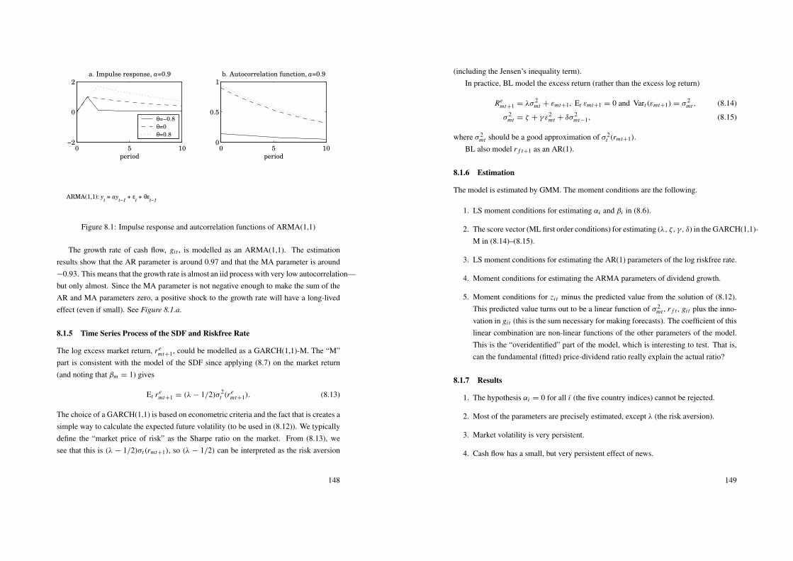
0 5 10−2

0

2

a. Impulse response, a=0.9

period

θ=−0.8

θ=0

θ=0.8

0 5 100

0.5

1

b. Autocorrelation function, a=0.9

period

ARMA(1,1): yt = ay

t−1 + ε

t + θε

t−1

Figure 8.1: Impulse response and autcorrelation functions of ARMA(1,1)

The growth rate of cash flow, gi t , is modelled as an ARMA(1,1). The estimationresults show that the AR parameter is around 0.97 and that the MA parameter is around−0.93. This means that the growth rate is almost an iid process with very low autocorrelation—but only almost. Since the MA parameter is not negative enough to make the sum of theAR and MA parameters zero, a positive shock to the growth rate will have a long-livedeffect (even if small). See Figure 8.1.a.

8.1.5 Time Series Process of the SDF and Riskfree Rate

The log excess market return, r emt+1, could be modelled as a GARCH(1,1)-M. The “M”

part is consistent with the model of the SDF since applying (8.7) on the market return(and noting that βm = 1) gives

Et r emt+1 = (λ− 1/2)σ 2

t (remt+1). (8.13)

The choice of a GARCH(1,1) is based on econometric criteria and the fact that is creates asimple way to calculate the expected future volatility (to be used in (8.12)). We typicallydefine the “market price of risk” as the Sharpe ratio on the market. From (8.13), wesee that this is (λ − 1/2)σt(rmt+1), so (λ − 1/2) can be interpreted as the risk aversion

148

(including the Jensen’s inequality term).In practice, BL model the excess return (rather than the excess log return)

Remt+1 = λσ 2

mt + εmt+1, Et εmt+1 = 0 and Vart(εmt+1) = σ 2mt , (8.14)

σ 2mt = ζ + γ ε2

mt + δσ 2mt−1, (8.15)

where σ 2mt should be a good approximation of σ 2

t (rmt+1).BL also model r f t+1 as an AR(1).

8.1.6 Estimation

The model is estimated by GMM. The moment conditions are the following.

1. LS moment conditions for estimating αi and βi in (8.6).

2. The score vector (ML first order conditions) for estimating (λ, ζ, γ, δ) in the GARCH(1,1)-M in (8.14)–(8.15).

3. LS moment conditions for estimating the AR(1) parameters of the log riskfree rate.

4. Moment conditions for estimating the ARMA parameters of dividend growth.

5. Moment conditions for zi t minus the predicted value from the solution of (8.12).This predicted value turns out to be a linear function of σ 2

mt , r f t , gi t plus the inno-vation in gi t (this is the sum necessary for making forecasts). The coefficient of thislinear combination are non-linear functions of the other parameters of the model.This is the “overidentified” part of the model, which is interesting to test. That is,can the fundamental (fitted) price-dividend ratio really explain the actual ratio?

8.1.7 Results

1. The hypothesis αi = 0 for all i (the five country indices) cannot be rejected.

2. Most of the parameters are precisely estimated, except λ (the risk aversion).

3. Market volatility is very persistent.

4. Cash flow has a small, but very persistent effect of news.

149

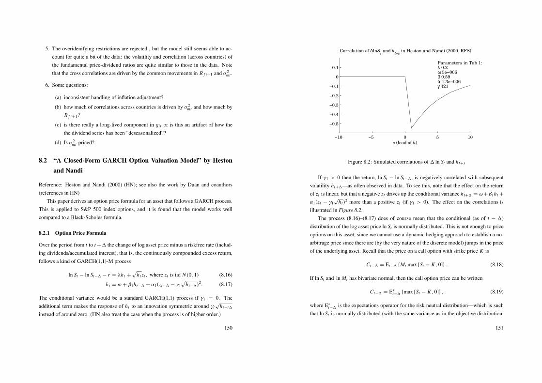
5. The overidenifying restrictions are rejected , but the model still seems able to ac-count for quite a bit of the data: the volatility and correlation (across countries) ofthe fundamental price-dividend ratios are quite similar to those in the data. Notethat the cross correlations are driven by the common movements in R f t+1 and σ 2

mt .

6. Some questions:

(a) inconsistent handling of inflation adjustment?

(b) how much of correlations across countries is driven by σ 2mt and how much by

R f t+1?

(c) is there really a long-lived component in gi t or is this an artifact of how thethe dividend series has been “deseasonalized”?

(d) Is σ 2mt priced?

8.2 “A Closed-Form GARCH Option Valuation Model” by Hestonand Nandi

Reference: Heston and Nandi (2000) (HN); see also the work by Duan and coauthors(references in HN)

This paper derives an option price formula for an asset that follows a GARCH process.This is applied to S&P 500 index options, and it is found that the model works wellcompared to a Black-Scholes formula.

8.2.1 Option Price Formula

Over the period from t to t +1 the change of log asset price minus a riskfree rate (includ-ing dividends/accumulated interest), that is, the continuously compounded excess return,follows a kind of GARCH(1,1)-M process

ln St − ln St−1 − r = λht +

√ht zt , where zt is iid N (0, 1) (8.16)

ht = ω + β1ht−1 + α1(zt−1 − γ1√

ht−1)2. (8.17)

The conditional variance would be a standard GARCH(1,1) process if γ1 = 0. Theadditional term makes the response of ht to an innovation symmetric around γi

√ht−i1

instead of around zero. (HN also treat the case when the process is of higher order.)

150

−10 −5 0 5 10

−0.5

−0.4

−0.3

−0.2

−0.1

0

0.1

Correlation of ∆lnSt and h

t+s in Heston and Nandi (2000, RFS)

s (lead of h)

Parameters in Tab 1:λ 0.2ω 5e−006β 0.59α 1.3e−006γ 421

Figure 8.2: Simulated correlations of 1 ln St and ht+s

If γ1 > 0 then the return, ln St − ln St−1, is negatively correlated with subsequentvolatility ht+1—as often observed in data. To see this, note that the effect on the returnof zt is linear, but that a negative zt drives up the conditional variance ht+1 = ω+β1ht +

α1(zt − γ1√

ht)2 more than a positive zt (if γ1 > 0). The effect on the correlations is

illustrated in Figure 8.2.The process (8.16)–(8.17) does of course mean that the conditional (as of t − 1)

distribution of the log asset price ln St is normally distributed. This is not enough to priceoptions on this asset, since we cannot use a dynamic hedging approach to establish a no-arbitrage price since there are (by the very nature of the discrete model) jumps in the priceof the underlying asset. Recall that the price on a call option with strike price K is

Ct−1 = Et−1 {Mt max [St − K , 0]} . (8.18)

If ln St and ln Mt has bivariate normal, then the call option price can be written

Ct−1 = E∗

t−1 {max [St − K , 0]} , (8.19)

where E∗

t−1 is the expectations operator for the risk neutral distribution—which is suchthat ln St is normally distributed (with the same variance as in the objective distribution,

151

but a different mean). This means that the Black-Scholes formula holds. See, for instance,Huang and Litzenberger (1988).

Remark 38 (Illustration of risk neutral distribution.) A risk neutral distribution is such

that the expected payoff equals today’s asset value. As an illustration, suppose the log

stochastic discount factor (mt = ln Mt ) and the log asset payoff (xt = ln X t ) have a

bivariate normal distribution (conditional on the information set in t − 1). The asset

price (Pt−1) is then

Pt−1 = Et−1 Mt X t = Et−1 exp (mt + xt)

= exp[Et−1 mt + Et−1 xt + Vart−1(mt)/2 + Vart−1(xt)/2 + Covt−1(mt , xt)

]= exp

[Et−1 mt + Vart−1(mt)/2

]exp

[Et−1 xt + Vart−1(xt)/2 + Covt−1(mt , xt)

].

For a real bond with a known payoff X t = 1, the last term is unity. Since the price of the

real bond is exp(−r f t−11

), we can rewrite the equation as

Pt−1 = exp(−r f t−11) exp[Et−1 xt + Covt−1(mt , xt)+ Vart−1(xt)/2

]= exp(−r f t−11)E∗

t−1 X t ,

where the distribution that defines the E∗

t−1 operator is such that ln X t = xt ∼ N [Et−1 xt+

Covt−1(mt , xt),Vart−1(xt)]. This shows that the risk neutral distribution has the same

variance, but a different mean. If the covariance is negative so the asset has a positive

risk premium (the price is low, see above), then the risk neutral distribution has a lower

mean than the objective distribution.

This is effectively what HN assume, since they assume that the risk neutral distributionis normal

Assumption: the price in t −1 of call option expiring in t follows BS.

HN show that the risk neutral process must then be as in (8.16)–(8.17), but with γ1

replaced by γ ∗

1 = γ1 +λ+1/2 and λ replaced by −1/2 (not in γ ∗

1 , of course). This meansthat they use the assumption about the conditional (as of t −1) distribution of St to buildup a conditional (as of t − 1) distribution of St+s for any s. It is clear that if we knowthat the risk neutral process is of the form (8.16)–(8.17), but with other parameters, then

152

we can calculate the risk neutral distribution for any horizon (by clever tricks or simplyby using (8.16)–(8.17) to do Monte Carlo simulations).

Once we have a risk neutral process it is (in principle, at least) straightforward toderive any option price (for any time to expiry). For a European call option with strikeprice K and expiry at date T , the result is

Ct(St , r, K , T ) = e−r(T −t) E∗

t max [ST − K , 0] (8.20)

= St P1 − e−r(T −t)K P2, (8.21)

where P1 and P2 are two risk neutral probabilities (implied by the risk neutral versionof (8.16)–(8.17), see above). It can be shown that P2 is the risk neutral probabilitythat ST > K , and that P1 is the delta, ∂Ct(St , r, K , T )/∂St . In practice, HN cal-culate these probabilities by first finding the risk neutral characteristic function of ST ,f (φ) = E∗

t exp(iφ ln ST ), where i2= −1, and then inverting to get the probabilities.

Remark 39 (Characteristic function and the pdf.) The characteristic function of a ran-

dom variable x is

f (φ) = E exp(iφx)

=∫

x exp(iφx)pdf(x)dx,

where pdf(x) is the pdf. This is a Fourier transform of the pdf (if x is a continuous random

variable). The pdf can therefore be recovered by the inverse Fourier transform as

pdf(x) =1

2π

∫∞

−∞exp(−iφx) f (φ)dφ.

8.2.2 Application to S&P 500 Index Option

Returns on the index are calculated by using official index plus dividends. The riskfreerate is taken to be a synthetic T-bill rate created by interpolating different bills to matchthe maturity of the option. Weekly data for 1992–1994 are used (created by using lots ofintraday quotes for all Wednesdays).

HN estimate the “GARCH(1,1)-M” process (8.16)–(8.17) with ML on daily data onthe S&P500 index returns. It is found that the βi parameter is large, αi is small, and thatγ1 > 0 (as expected). The latter seems to be important for the estimated ht series (seeFigures 1 and 2).

153

Instead of using the “GARCH(1,1)-M” process estimated from the S&P500 indexreturns, all the model parameters are subsequently estimated from option prices. Recallthat the probabilities P1 and P2 in (8.21) depend (nonlinearly) on the parameters of therisk neutral version of (8.16)-(8.17). The model parameters can therefore be estimated byminimizing the sum (across option price observation) squared pricing errors.

In one of several different estimations, HN estimate the model on option data forthe first half 1992 and then evaluate the model by comparing implied and actual optionprices for the second half of 1992. These implied option prices use the model parametersestimated on data for the first half of the year and an estimate of ht calculated usingthese parameters and the latest S&P 500 index returns. The performance of this model iscompared with a Black-Scholes model (among other models,) where the implied volatilityin week t − 1 is used to price options in price t . This exercise is repeated for 1993 and1994.

It is found that the GARCH model outperforms (in terms of MSE) the B-S model. Inparticular, it seems as if the GARCH model gives much smaller errors for deep out-of-the-money options (see Figures 2 and 3). HN argue that this is due to two aspects of themodel: the time-profile of volatility (somewhat persistent, but mean-reverting) and thenegative correlation of returns and volatility.

Bibliography

Bansal, R., and C. Lundblad, 2002, “Market Efficiency, Fundamental Values, and theSize of the Risk Premium in Global Equity Markets,” Journal of Econometrics, 109,195–237.

Heston, S. L., and S. Nandi, 2000, “A Closed-Form GARCH Option Valuation Model,”Review of Financial Studies, 13, 585–625.

Huang, C.-F., and R. H. Litzenberger, 1988, Foundations for Financial Economics, Else-vier Science Publishing, New York.

154

9 Models of Short Interest Rates

9.1 SDF and Yield Curve Models

A yield curve model is essentially a model for the conditional mean of the SDF. Thissection summarizes some basic results.

9.1.1 Preliminaries

Reference: Cochrane (2001) 19.3; Campbell, Lo, and MacKinlay (1997) 11.1The price in t of a bill paying 1 unit of account (for sure) in t + n is

Pnt = Et Mt+1Mt+2 . . .Mt+n1 = Et exp(mt+1 + mt+2 + . . .+ mt+n)1, (9.1)

where mt+1 is the log SDF. (To see this note that P2t = Et Mt+1 P1t+1 and that P1t+1 =

Et+1 Mt+21. Combining gives P2t = Et Mt+1 Et+1 Mt+2 = Et Mt+1Mt+2 by iteratedexpectations.)

A continuously compounded n-period interest rate, ynt satisfies

exp(−nynt) = Pnt . (9.2)

The SDF is a real SDF if the interest rates are real, otherwise it is a nominal SDF.

9.1.2 When the log SDF is Normally Distributed

Assume that mt+1 + mt+2 + . . .+ mt+n in (9.1) is conditionally normally distributed

(mt+1 + mt+2 + . . .+ mt+n)|�t ∼ N [µnt , s2nt ]. (9.3)

We can then evaluate (9.1)–(9.2) as

exp(−nynt) = Pnt = Et exp(mt+1 + mt+2 + . . .+ mt+n) = exp(µnt + s2nt/2), or

ynt = −µnt

n−

s2nt

2n. (9.4)

155

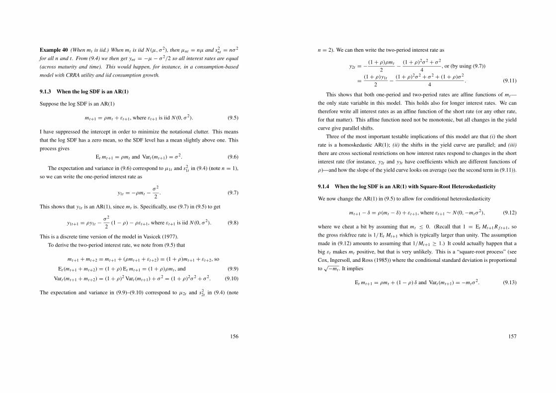
Example 40 (When mt is iid.) When mt is iid N (µ, σ 2), then µnt = nµ and s2nt = nσ 2

for all n and t. From (9.4) we then get ynt = −µ − σ 2/2 so all interest rates are equal

(across maturity and time). This would happen, for instance, in a consumption-based

model with CRRA utility and iid consumption growth.

9.1.3 When the log SDF is an AR(1)

Suppose the log SDF is an AR(1)

mt+1 = ρmt + εt+1, where εt+1 is iid N (0, σ 2). (9.5)

I have suppressed the intercept in order to minimize the notational clutter. This meansthat the log SDF has a zero mean, so the SDF level has a mean slightly above one. Thisprocess gives

Et mt+1 = ρmt and Vart(mt+1) = σ 2. (9.6)

The expectation and variance in (9.6) correspond to µ1t and s21t in (9.4) (note n = 1),

so we can write the one-period interest rate as

y1t = −ρmt −σ 2

2. (9.7)

This shows that y1t is an AR(1), since mt is. Specifically, use (9.7) in (9.5) to get

y1t+1 = ρy1t −σ 2

2(1 − ρ)− ρεt+1, where εt+1 is iid N (0, σ 2). (9.8)

This is a discrete time version of the model in Vasicek (1977).To derive the two-period interest rate, we note from (9.5) that

mt+1 + mt+2 = mt+1 + (ρmt+1 + εt+2) = (1 + ρ)mt+1 + εt+2, so

Et(mt+1 + mt+2) = (1 + ρ)Et mt+1 = (1 + ρ)ρmt , and (9.9)

Vart(mt+1 + mt+2) = (1 + ρ)2 Vart(mt+1)+ σ 2= (1 + ρ)2σ 2

+ σ 2. (9.10)

The expectation and variance in (9.9)–(9.10) correspond to µ2t and s22t in (9.4) (note

156

n = 2). We can then write the two-period interest rate as

y2t = −(1 + ρ)ρmt

2−(1 + ρ)2σ 2

+ σ 2

4, or (by using (9.7))

=(1 + ρ)y1t

2−(1 + ρ)2σ 2

+ σ 2+ (1 + ρ)σ 2

4. (9.11)

This shows that both one-period and two-period rates are affine functions of mt—the only state variable in this model. This holds also for longer interest rates. We cantherefore write all interest rates as an affine function of the short rate (or any other rate,for that matter). This affine function need not be monotonic, but all changes in the yieldcurve give parallel shifts.

Three of the most important testable implications of this model are that (i) the shortrate is a homoskedastic AR(1); (ii) the shifts in the yield curve are parallel; and (iii)

there are cross sectional restrictions on how interest rates respond to changes in the shortinterest rate (for instance, y2t and y3t have coefficients which are different functions ofρ)—and how the slope of the yield curve looks on average (see the second term in (9.11)).

9.1.4 When the log SDF is an AR(1) with Square-Root Heteroskedasticity

We now change the AR(1) in (9.5) to allow for conditional heteroskedasticity

mt+1 − δ = ρ(mt − δ)+ εt+1, where εt+1 ∼ N (0,−mtσ2), (9.12)

where we cheat a bit by assuming that mt ≤ 0. (Recall that 1 = Et Mt+1 R f t+1, sothe gross riskfree rate is 1/Et Mt+1 which is typically larger than unity. The assumptionmade in (9.12) amounts to assuming that 1/Mt+1 ≥ 1.) It could actually happen that abig εt makes mt positive, but that is very unlikely. This is a “square-root process” (seeCox, Ingersoll, and Ross (1985)) where the conditional standard deviation is proportionalto

√−mt . It implies

Et mt+1 = ρmt + (1 − ρ) δ and Vart(mt+1) = −mtσ2. (9.13)

157

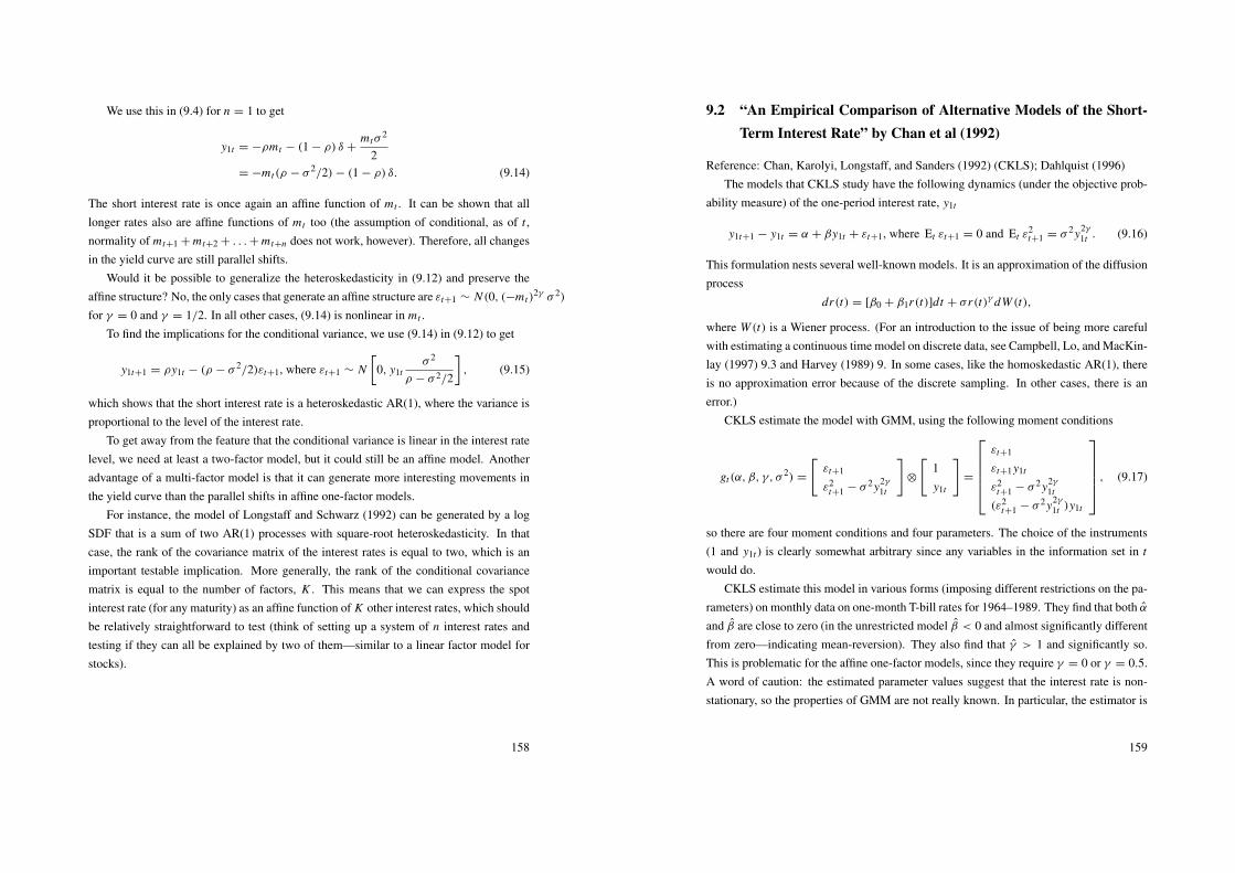
We use this in (9.4) for n = 1 to get

y1t = −ρmt − (1 − ρ) δ +mtσ

2

2= −mt(ρ − σ 2/2)− (1 − ρ) δ. (9.14)

The short interest rate is once again an affine function of mt . It can be shown that alllonger rates also are affine functions of mt too (the assumption of conditional, as of t ,normality of mt+1 + mt+2 + . . .+ mt+n does not work, however). Therefore, all changesin the yield curve are still parallel shifts.

Would it be possible to generalize the heteroskedasticity in (9.12) and preserve theaffine structure? No, the only cases that generate an affine structure are εt+1 ∼ N (0, (−mt)

2γ σ 2)

for γ = 0 and γ = 1/2. In all other cases, (9.14) is nonlinear in mt .To find the implications for the conditional variance, we use (9.14) in (9.12) to get

y1t+1 = ρy1t − (ρ − σ 2/2)εt+1, where εt+1 ∼ N[

0, y1tσ 2

ρ − σ 2/2

], (9.15)

which shows that the short interest rate is a heteroskedastic AR(1), where the variance isproportional to the level of the interest rate.

To get away from the feature that the conditional variance is linear in the interest ratelevel, we need at least a two-factor model, but it could still be an affine model. Anotheradvantage of a multi-factor model is that it can generate more interesting movements inthe yield curve than the parallel shifts in affine one-factor models.

For instance, the model of Longstaff and Schwarz (1992) can be generated by a logSDF that is a sum of two AR(1) processes with square-root heteroskedasticity. In thatcase, the rank of the covariance matrix of the interest rates is equal to two, which is animportant testable implication. More generally, the rank of the conditional covariancematrix is equal to the number of factors, K . This means that we can express the spotinterest rate (for any maturity) as an affine function of K other interest rates, which shouldbe relatively straightforward to test (think of setting up a system of n interest rates andtesting if they can all be explained by two of them—similar to a linear factor model forstocks).

158

9.2 “An Empirical Comparison of Alternative Models of the Short-Term Interest Rate” by Chan et al (1992)

Reference: Chan, Karolyi, Longstaff, and Sanders (1992) (CKLS); Dahlquist (1996)The models that CKLS study have the following dynamics (under the objective prob-

ability measure) of the one-period interest rate, y1t

y1t+1 − y1t = α + βy1t + εt+1, where Et εt+1 = 0 and Et ε2t+1 = σ 2y2γ

1t . (9.16)

This formulation nests several well-known models. It is an approximation of the diffusionprocess

dr(t) = [β0 + β1r(t)]dt + σr(t)γ dW (t),

where W (t) is a Wiener process. (For an introduction to the issue of being more carefulwith estimating a continuous time model on discrete data, see Campbell, Lo, and MacKin-lay (1997) 9.3 and Harvey (1989) 9. In some cases, like the homoskedastic AR(1), thereis no approximation error because of the discrete sampling. In other cases, there is anerror.)

CKLS estimate the model with GMM, using the following moment conditions

gt(α, β, γ, σ2) =

[εt+1

ε2t+1 − σ 2y2γ

1t

]⊗

[1y1t

]=

εt+1

εt+1y1t

ε2t+1 − σ 2y2γ

1t

(ε2t+1 − σ 2y2γ

1t )y1t

, (9.17)

so there are four moment conditions and four parameters. The choice of the instruments(1 and y1t ) is clearly somewhat arbitrary since any variables in the information set in t

would do.CKLS estimate this model in various forms (imposing different restrictions on the pa-

rameters) on monthly data on one-month T-bill rates for 1964–1989. They find that both αand β are close to zero (in the unrestricted model β < 0 and almost significantly differentfrom zero—indicating mean-reversion). They also find that γ > 1 and significantly so.This is problematic for the affine one-factor models, since they require γ = 0 or γ = 0.5.A word of caution: the estimated parameter values suggest that the interest rate is non-stationary, so the properties of GMM are not really known. In particular, the estimator is

159

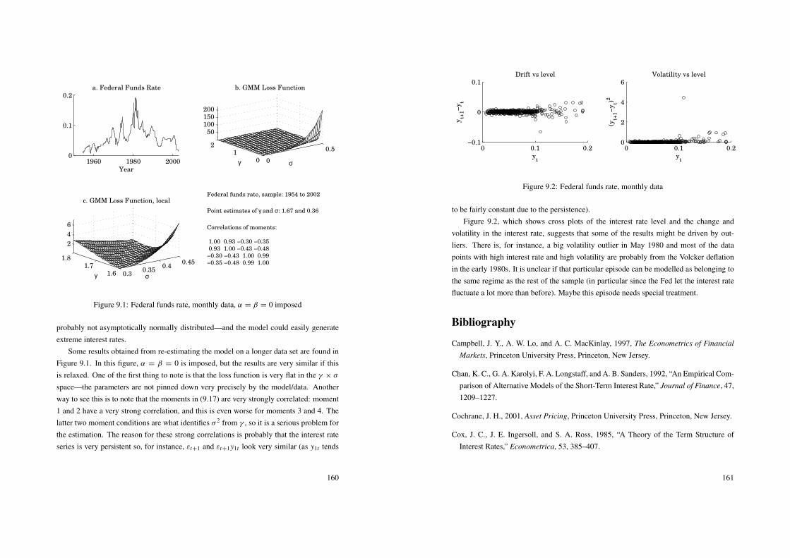
1960 1980 20000

0.1

0.2a. Federal Funds Rate

Year

0

0.5

01

2

50100150200

σ

b. GMM Loss Function

γ

0.30.35

0.40.45

1.61.7

1.8

2

4

6

σ

c. GMM Loss Function, local

γ

Federal funds rate, sample: 1954 to 2002

Point estimates of γ and σ: 1.67 and 0.36

Correlations of moments:

1.00 0.93 −0.30 −0.35

0.93 1.00 −0.43 −0.48

−0.30 −0.43 1.00 0.99

−0.35 −0.48 0.99 1.00

Figure 9.1: Federal funds rate, monthly data, α = β = 0 imposed

probably not asymptotically normally distributed—and the model could easily generateextreme interest rates.

Some results obtained from re-estimating the model on a longer data set are found inFigure 9.1. In this figure, α = β = 0 is imposed, but the results are very similar if thisis relaxed. One of the first thing to note is that the loss function is very flat in the γ × σ

space—the parameters are not pinned down very precisely by the model/data. Anotherway to see this is to note that the moments in (9.17) are very strongly correlated: moment1 and 2 have a very strong correlation, and this is even worse for moments 3 and 4. Thelatter two moment conditions are what identifies σ 2 from γ , so it is a serious problem forthe estimation. The reason for these strong correlations is probably that the interest rateseries is very persistent so, for instance, εt+1 and εt+1y1t look very similar (as y1t tends

160

0 0.1 0.2−0.1

0

0.1Drift vs level

yt

yt+

1−

yt

0 0.1 0.20

2

4

6Volatility vs level

yt

(yt+

1−

yt)2

Figure 9.2: Federal funds rate, monthly data

to be fairly constant due to the persistence).Figure 9.2, which shows cross plots of the interest rate level and the change and

volatility in the interest rate, suggests that some of the results might be driven by out-liers. There is, for instance, a big volatility outlier in May 1980 and most of the datapoints with high interest rate and high volatility are probably from the Volcker deflationin the early 1980s. It is unclear if that particular episode can be modelled as belonging tothe same regime as the rest of the sample (in particular since the Fed let the interest ratefluctuate a lot more than before). Maybe this episode needs special treatment.

Bibliography

Campbell, J. Y., A. W. Lo, and A. C. MacKinlay, 1997, The Econometrics of Financial

Markets, Princeton University Press, Princeton, New Jersey.

Chan, K. C., G. A. Karolyi, F. A. Longstaff, and A. B. Sanders, 1992, “An Empirical Com-parison of Alternative Models of the Short-Term Interest Rate,” Journal of Finance, 47,1209–1227.

Cochrane, J. H., 2001, Asset Pricing, Princeton University Press, Princeton, New Jersey.

Cox, J. C., J. E. Ingersoll, and S. A. Ross, 1985, “A Theory of the Term Structure ofInterest Rates,” Econometrica, 53, 385–407.

161

Dahlquist, M., 1996, “On Alternative Interest Rate Processes,” Journal of Banking and

Finance, 20, 1093–1119.

Harvey, A. C., 1989, Forecasting, Structural Time Series Models and the Kalman Filter,Cambridge University Press.

Longstaff, F. A., and E. S. Schwarz, 1992, “Interest Rate Volatility and the Term Structure:A Two-Factor General Equilibrium Model,” Journal of Finance, 47, 1259–1282.

Vasicek, O. A., 1977, “An Equilibrium Characterization of the Term Structure,” Journal

of Financial Economics, 5, 177–188.

162

10 Kernel Density Estimation and Regression

10.1 Non-Parametric Regression

Reference: Campbell, Lo, and MacKinlay (1997) 12.3; Hardle (1990); Pagan and Ullah(1999)

10.1.1 Simple Kernel Regression

Non-parametric regressions are used when we are unwilling to impose a parametric formon the regression equation—and we have a lot of data.

Let the scalars yt and xt be related as

yt = m(xt)+ εt , εt is iid and E εt = Cov [m(xt), εt ] = 0, (10.1)

where m() is a, possibly non-linear, function.Suppose the sample had 3 observations (say, t = 3, 27, and 99) with exactly the same

value of xt , say 2.1. A natural way of estimating m(x) at x = 2.1 would then be toaverage over these 3 observations as we can expect average of the error terms to be closeto zero (iid and zero mean).

Unfortunately, we seldom have repeated observations of this type. Instead, we maytry to approximate the value of m(x) (x is a single value, 1.9, say) by averaging overobservations where xt is close to x . The general form of this type of estimator is

m(x) =

∑Tt=1w(xt − x)yt∑T

t=1w(xt − x), (10.2)

where w(xt − x)/6Tt=1w(xt − x) is the weight given to observation t . Note that denomi-

nator makes the weights sum to unity.As an example of a w(.) function, it could give equal weight to the k values of xt

which are closest to x and zero weight to all other observations (this is the “k-nearestneighbor” estimator, see Hardle (1990) 3.2). As another example, the weight functioncould be defined so that it trades off the expected squared errors, E[yt − m(x)]2, and the

163

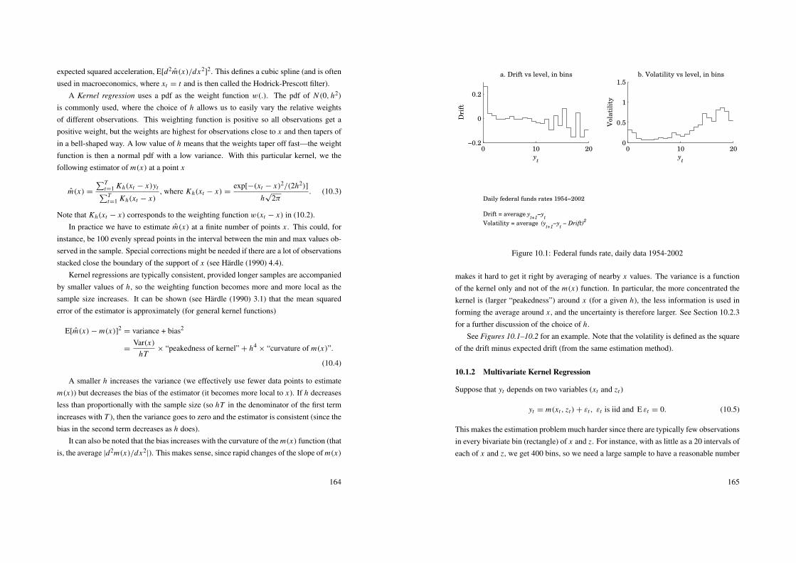
expected squared acceleration, E[d2m(x)/dx2]2. This defines a cubic spline (and is often

used in macroeconomics, where xt = t and is then called the Hodrick-Prescott filter).A Kernel regression uses a pdf as the weight function w(.). The pdf of N (0, h2)

is commonly used, where the choice of h allows us to easily vary the relative weightsof different observations. This weighting function is positive so all observations get apositive weight, but the weights are highest for observations close to x and then tapers ofin a bell-shaped way. A low value of h means that the weights taper off fast—the weightfunction is then a normal pdf with a low variance. With this particular kernel, we thefollowing estimator of m(x) at a point x

m(x) =

∑Tt=1 Kh(xt − x)yt∑T

t=1 Kh(xt − x), where Kh(xt − x) =

exp[−(xt − x)2/(2h2)]

h√

2π. (10.3)

Note that Kh(xt − x) corresponds to the weighting function w(xt − x) in (10.2).In practice we have to estimate m(x) at a finite number of points x . This could, for

instance, be 100 evenly spread points in the interval between the min and max values ob-served in the sample. Special corrections might be needed if there are a lot of observationsstacked close the boundary of the support of x (see Hardle (1990) 4.4).

Kernel regressions are typically consistent, provided longer samples are accompaniedby smaller values of h, so the weighting function becomes more and more local as thesample size increases. It can be shown (see Hardle (1990) 3.1) that the mean squarederror of the estimator is approximately (for general kernel functions)

E[m(x)− m(x)]2= variance + bias2

=Var(x)

hT× “peakedness of kernel” + h4

× “curvature of m(x)”.

(10.4)

A smaller h increases the variance (we effectively use fewer data points to estimatem(x)) but decreases the bias of the estimator (it becomes more local to x). If h decreasesless than proportionally with the sample size (so hT in the denominator of the first termincreases with T ), then the variance goes to zero and the estimator is consistent (since thebias in the second term decreases as h does).

It can also be noted that the bias increases with the curvature of the m(x) function (thatis, the average |d2m(x)/dx2

|). This makes sense, since rapid changes of the slope of m(x)

164

0 10 20−0.2

0

0.2

a. Drift vs level, in bins

yt

Dri

ft

0 10 200

0.5

1

1.5b. Volatility vs level, in bins

yt

Vola

tili

ty

Daily federal funds rates 1954−2002

Drift = average yt+1

−yt

Volatility = average (yt+1

−yt − Drift)

2

Figure 10.1: Federal funds rate, daily data 1954-2002

makes it hard to get it right by averaging of nearby x values. The variance is a functionof the kernel only and not of the m(x) function. In particular, the more concentrated thekernel is (larger “peakedness”) around x (for a given h), the less information is used informing the average around x , and the uncertainty is therefore larger. See Section 10.2.3for a further discussion of the choice of h.

See Figures 10.1–10.2 for an example. Note that the volatility is defined as the squareof the drift minus expected drift (from the same estimation method).

10.1.2 Multivariate Kernel Regression

Suppose that yt depends on two variables (xt and zt )

yt = m(xt , zt)+ εt , εt is iid and E εt = 0. (10.5)

This makes the estimation problem much harder since there are typically few observationsin every bivariate bin (rectangle) of x and z. For instance, with as little as a 20 intervals ofeach of x and z, we get 400 bins, so we need a large sample to have a reasonable number

165

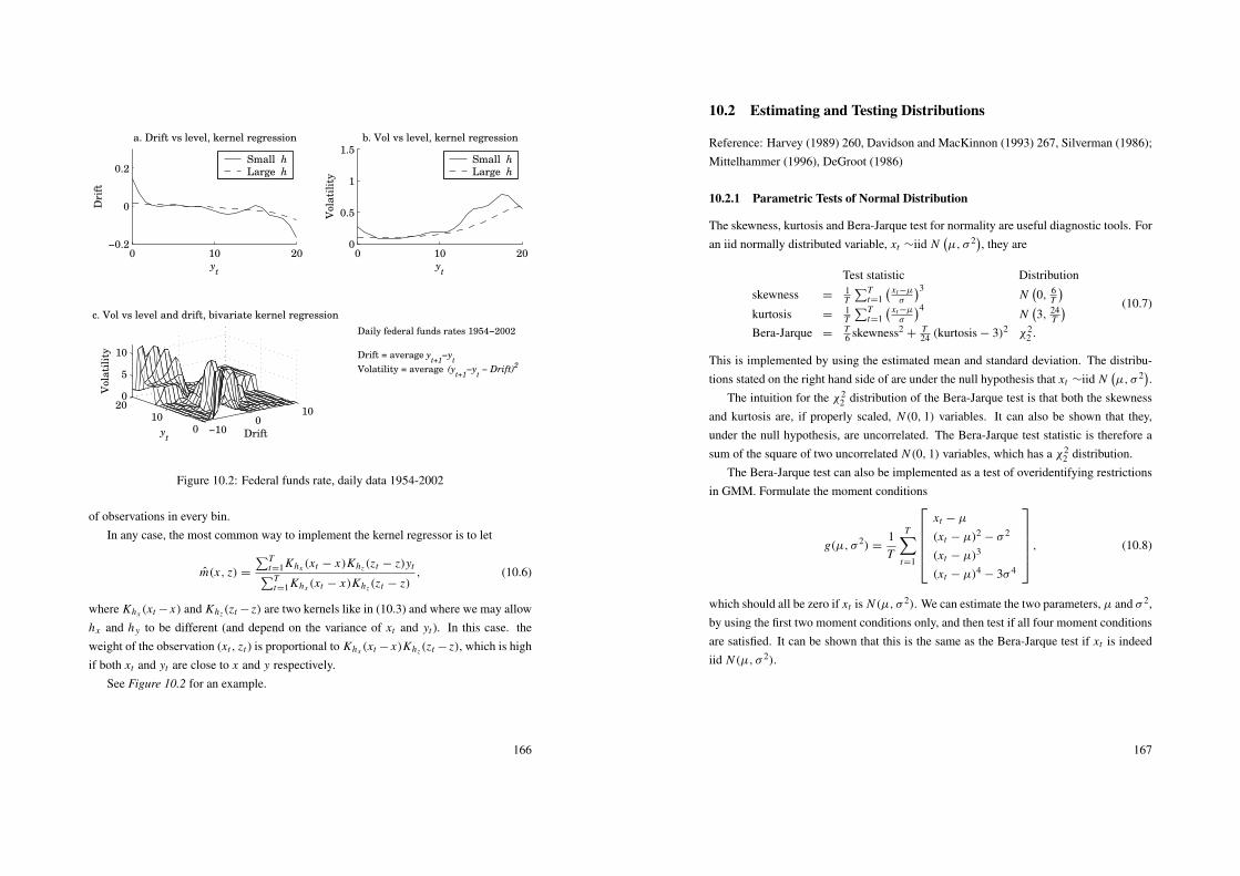
0 10 20−0.2

0

0.2

a. Drift vs level, kernel regression

yt

Dri

ft

Small h

Large h

0 10 200

0.5

1

1.5b. Vol vs level, kernel regression

yt

Vola

tili

ty

Small h

Large h

−100

10

010

200

5

10

Drift

c. Vol vs level and drift, bivariate kernel regression

yt

Vola

tili

ty

Daily federal funds rates 1954−2002

Drift = average yt+1

−yt

Volatility = average (yt+1

−yt − Drift)

2

Figure 10.2: Federal funds rate, daily data 1954-2002

of observations in every bin.In any case, the most common way to implement the kernel regressor is to let

m(x, z) =

∑Tt=1Khx (xt − x)Khz(zt − z)yt∑T

t=1Khx (xt − x)Khz(zt − z), (10.6)

where Khx (xt − x) and Khz(zt − z) are two kernels like in (10.3) and where we may allowhx and h y to be different (and depend on the variance of xt and yt ). In this case. theweight of the observation (xt , zt ) is proportional to Khx (xt − x)Khz(zt − z), which is highif both xt and yt are close to x and y respectively.

See Figure 10.2 for an example.

166

10.2 Estimating and Testing Distributions

Reference: Harvey (1989) 260, Davidson and MacKinnon (1993) 267, Silverman (1986);Mittelhammer (1996), DeGroot (1986)

10.2.1 Parametric Tests of Normal Distribution

The skewness, kurtosis and Bera-Jarque test for normality are useful diagnostic tools. Foran iid normally distributed variable, xt ∼iid N

(µ, σ 2), they are

Test statistic Distribution

skewness =1T∑T

t=1( xt−µ

σ

)3N(0, 6

T

)kurtosis =

1T∑T

t=1( xt−µ

σ

)4N(3, 24

T

)Bera-Jarque =

T6 skewness2

+T24 (kurtosis − 3)2 χ2

2 .

(10.7)

This is implemented by using the estimated mean and standard deviation. The distribu-tions stated on the right hand side of are under the null hypothesis that xt ∼iid N

(µ, σ 2).

The intuition for the χ22 distribution of the Bera-Jarque test is that both the skewness

and kurtosis are, if properly scaled, N (0, 1) variables. It can also be shown that they,under the null hypothesis, are uncorrelated. The Bera-Jarque test statistic is therefore asum of the square of two uncorrelated N (0, 1) variables, which has a χ2

2 distribution.The Bera-Jarque test can also be implemented as a test of overidentifying restrictions

in GMM. Formulate the moment conditions

g(µ, σ 2) =1T

T∑t=1

xt − µ

(xt − µ)2 − σ 2

(xt − µ)3

(xt − µ)4 − 3σ 4

, (10.8)

which should all be zero if xt is N (µ, σ 2). We can estimate the two parameters, µ and σ 2,by using the first two moment conditions only, and then test if all four moment conditionsare satisfied. It can be shown that this is the same as the Bera-Jarque test if xt is indeediid N (µ, σ 2).

167

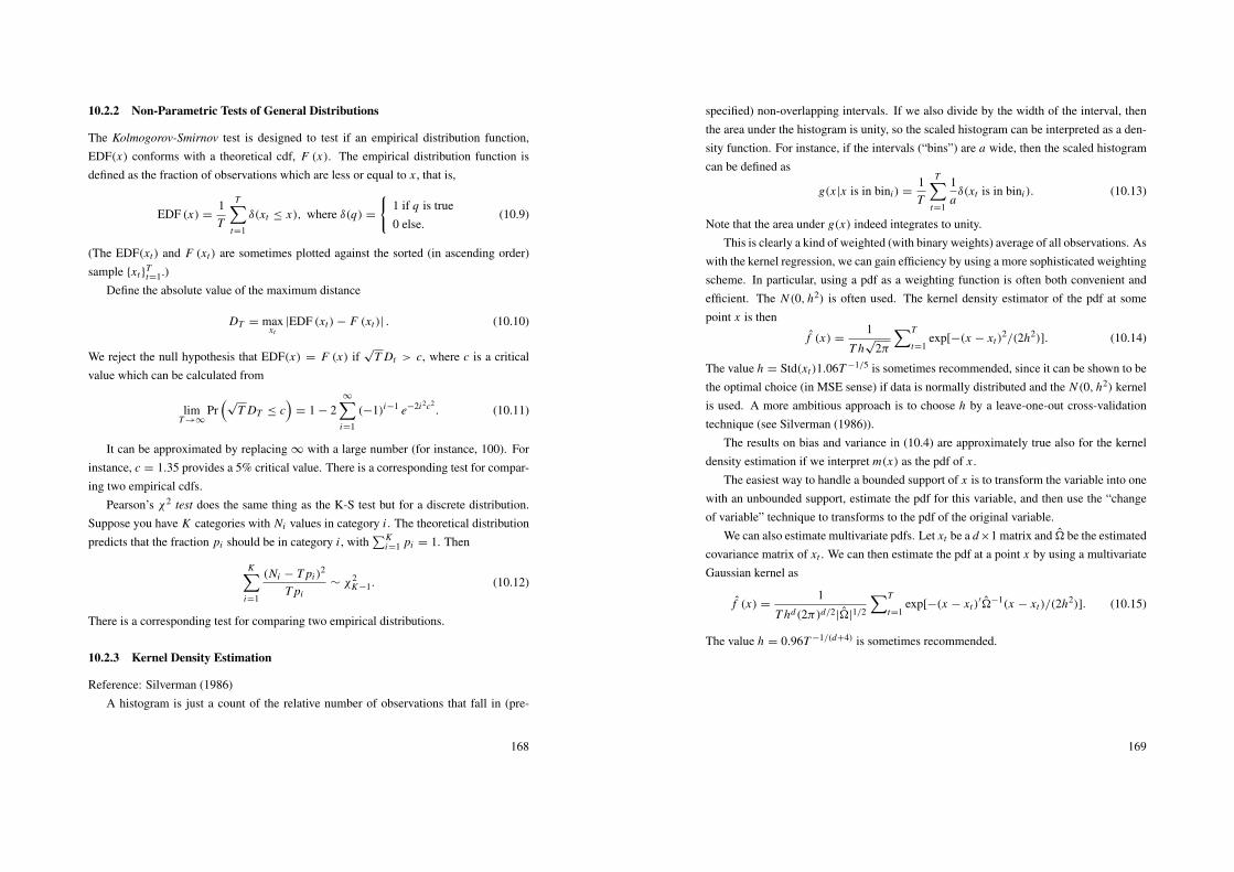
10.2.2 Non-Parametric Tests of General Distributions

The Kolmogorov-Smirnov test is designed to test if an empirical distribution function,EDF(x) conforms with a theoretical cdf, F (x). The empirical distribution function isdefined as the fraction of observations which are less or equal to x , that is,

EDF (x) =1T

T∑t=1

δ(xt ≤ x), where δ(q) =

{1 if q is true0 else.

(10.9)

(The EDF(xt) and F (xt) are sometimes plotted against the sorted (in ascending order)sample {xt}

Tt=1.)

Define the absolute value of the maximum distance

DT = maxxt

|EDF (xt)− F (xt)| . (10.10)

We reject the null hypothesis that EDF(x) = F (x) if√

T Dt > c, where c is a criticalvalue which can be calculated from

limT →∞

Pr(√

T DT ≤ c)

= 1 − 2∞∑

i=1

(−1)i−1 e−2i2c2. (10.11)

It can be approximated by replacing ∞ with a large number (for instance, 100). Forinstance, c = 1.35 provides a 5% critical value. There is a corresponding test for compar-ing two empirical cdfs.

Pearson’s χ2 test does the same thing as the K-S test but for a discrete distribution.Suppose you have K categories with Ni values in category i . The theoretical distributionpredicts that the fraction pi should be in category i , with

∑Ki=1 pi = 1. Then

K∑i=1

(Ni − T pi )2

T pi∼ χ2

K−1. (10.12)

There is a corresponding test for comparing two empirical distributions.

10.2.3 Kernel Density Estimation

Reference: Silverman (1986)A histogram is just a count of the relative number of observations that fall in (pre-

168

specified) non-overlapping intervals. If we also divide by the width of the interval, thenthe area under the histogram is unity, so the scaled histogram can be interpreted as a den-sity function. For instance, if the intervals (“bins”) are a wide, then the scaled histogramcan be defined as

g(x |x is in bini ) =1T

T∑t=1

1aδ(xt is in bini ). (10.13)

Note that the area under g(x) indeed integrates to unity.This is clearly a kind of weighted (with binary weights) average of all observations. As

with the kernel regression, we can gain efficiency by using a more sophisticated weightingscheme. In particular, using a pdf as a weighting function is often both convenient andefficient. The N (0, h2) is often used. The kernel density estimator of the pdf at somepoint x is then

f (x) =1

T h√

2π

∑T

t=1exp[−(x − xt)

2/(2h2)]. (10.14)

The value h = Std(xt)1.06T −1/5 is sometimes recommended, since it can be shown to bethe optimal choice (in MSE sense) if data is normally distributed and the N (0, h2) kernelis used. A more ambitious approach is to choose h by a leave-one-out cross-validationtechnique (see Silverman (1986)).

The results on bias and variance in (10.4) are approximately true also for the kerneldensity estimation if we interpret m(x) as the pdf of x .

The easiest way to handle a bounded support of x is to transform the variable into onewith an unbounded support, estimate the pdf for this variable, and then use the “changeof variable” technique to transforms to the pdf of the original variable.

We can also estimate multivariate pdfs. Let xt be a d×1 matrix and � be the estimatedcovariance matrix of xt . We can then estimate the pdf at a point x by using a multivariateGaussian kernel as

f (x) =1

T hd(2π)d/2|�|1/2

∑T

t=1exp[−(x − xt)

′�−1(x − xt)/(2h2)]. (10.15)

The value h = 0.96T −1/(d+4) is sometimes recommended.

169

0 10 200

0.1

0.2a. Histogram (scaled: area=1)

yt

0 10 200

0.1

0.2b. Kernel density estimation

yt

Small h

Medium h

Large h

Daily federal funds rates 1954−2002

K−S (against N(µ,σ2)): sqrt(T)D = 14.9

Skewness: 1.258

kurtosis: 5.22

Bera−Jarque: 8301

Figure 10.3: Federal funds rate, daily data 1954-2002

10.3 “Testing Continuous-Time Models of the Spot Interest Rate,”by Ait-Sahalia (1996)

Reference: Ait-Sahalia (1996)This paper tests several models of the short interest rate by using a non-parametric

technique.

1. The first step of the analysis is to estimate the unconditional distribution of theshort interest rate by a kernel density estimator like (10.14). The estimated pdf atthe value r is denoted π0(r).

2. The second step is to estimate the parameters in a short rate model (for instance,Vasicek’s model) by making the unconditional distribution implied by the modelparameters (denoted π(θ, r) where θ is a vector of the model parameters and r avalue of the short rate) as close as possible to the non-parametric estimate obtained

170

in step 1. This is done by choosing the model parameters as

θ = arg minθ

1T

T∑t=1

[π(θ, rt)− π0(r)]2. (10.16)

3. The model is tested by using a scaled version of the minimized value of the righthand side of (10.16) as a test statistic (it has an asymptotic normal distribution).

4. It is found that most standard models are rejected (daily data on 7-day Eurodollardeposit rate, June 1973 to February 1995, 5,500 observations), mostly because ac-tual mean reversion is much more non-linear in the interest rate level than suggestedby most models. The actual drift and volatility are much like those in Figure 10.2.

10.4 “Nonparametric Estimation of Stat-Price Densities Implicit inFinancial Asset Prices,” by Ait-Sahalia and Lo (1998)

Reference: Ait-Sahalia and Lo (1998)This paper estimates non-parametric option price functions and calculates the implicit

risk-neutral distribution as the second partial derivative of this function with respect to thestrike price.

1. First, the call option price, Hi t , is estimated as a multivariate kernel regression

Hi t = m(St , X, τ, rτ t , δτ t)+ εi t , (10.17)

where St is the price of the underlying asset, X is the strike price, τ is time toexpiry, rτ t is the interest rate between t and t + τ , and δτ t is the dividend yield(if any) between t and t + τ . It is very hard to estimate a five-dimensional kernelregression, so various ways of reducing the dimensionality are tried. For instance,by making m() a function of the forward price, St [τ exp(rτ t − δτ t)], instead of St ,rτ t , and δτ t separably.

2. Second, the implicit riskneutral pdf of the future asset price is calculated as∂2m(St , X, τ, rτ t , δτ t)/∂X2, properly scaled so it integrates to unity.

171

3. This approach is used on daily data for Jan 1993 to Dec 1993 on S&P 500 index op-tions (14,000 observations). They find interesting patterns of the implied moments(mean, volatility, skewness, and kurtosis) as the time to expiry changes. In par-ticular, the non-parametric estimates suggest that distributions for longer horizonshave increasingly larger skewness and kurtosis: whereas the distributions for shorthorizons are not too different from normal distributions, this is not true for longerhorizons. (See their Fig 7.)

4. They also argue that there is little evidence of instability in the implicit pdf overtheir sample.

Bibliography

Ait-Sahalia, Y., 1996, “Testing Continuous-Time Models of the Spot Interest Rate,” Re-

view of Financial Studies, 9, 385–426.

Ait-Sahalia, Y., and A. W. Lo, 1998, “Nonparametric Estimation of Stat-Price DensitiesImplicit in Financial Asset Prices,” Journal of Finance, 53, 499–547.

Campbell, J. Y., A. W. Lo, and A. C. MacKinlay, 1997, The Econometrics of Financial

Markets, Princeton University Press, Princeton, New Jersey.

Davidson, R., and J. G. MacKinnon, 1993, Estimation and Inference in Econometrics,Oxford University Press, Oxford.

DeGroot, M. H., 1986, Probability and Statistics, Addison-Wesley, Reading, Mas-sachusetts.

Hardle, W., 1990, Applied Nonparametric Regression, Cambridge University Press, Cam-bridge.

Harvey, A. C., 1989, Forecasting, Structural Time Series Models and the Kalman Filter,Cambridge University Press.

Mittelhammer, R. C., 1996, Mathematical Statistics for Economics and Business,Springer-Verlag, New York.

172

Pagan, A., and A. Ullah, 1999, Nonparametric Econometrics, Cambridge UniversityPress.

Silverman, B. W., 1986, Density Estimation for Statistics and Data Analysis, Chapmanand Hall, London.

173

21 Finite-difference Solution of Option Prices

21.1 Black-Scholes

We are interested in the price of a European call option with strike price K . The price ofthe underlying asset follows a geometric Brownian motion

dx (t) = αx (t) dt + σ x (t) dW (t) , (21.1)

where W (t) is a Wiener process. Suppose the risk free rate is a constant, r . The notation(for instance, that the underlying asset price is denoted by x) follows the convention inmost texts on finite-difference methods.

Equilibrium requires that the option price function, C (x, t) satisfies the followingpartial differential equation (PDE)

0 = −rC (x, t)+∂C (x, t)∂t

+ r x (t)∂C (x, t)∂x

+12

x (t)2 σ 2 ∂2C (x, t)∂x2 , (21.2)

with the boundary conditions (at expiration date T )

C (x, T ) = max [x (T )− K , 0] . (21.3)

We know that the solution is

C (x, t) = x (t)8 (d1)− e−r(T −t)K8(

d1 − σ√

T − t)

, where (21.4)

d1 =ln [x (t) /K ] +

(r + σ 2/2

)(T − t)

σ√

T − t.

It will also turn out to be useful to note that

C (0, t) = 0 and limx→∞ C (x, t) = limx→∞ x − e−r(T −t)K . (21.5)

174

21.2 Finite-difference Methods

References: Duffie (1992), appendix 10.H; Wilmott, Howison, and Dewynne (1995) 8;Press, Teukolsky, Vetterling, and Flannery (1992) 19.2; Hull (2000) 16.8

The partial differential equation we will solve for F (x, t) is

0 = −r (x, t) F (x, t)+∂F (x, t)∂t

+µ (x, t)∂F (x, t)∂x

+12σ (x, t)2

∂2 F (x, t)∂x2 +h (x, t) .

(21.6)This is more general than the Black-Scholes model, and will allow us to price more com-plicated derivatives.

Example 41 (The Black-Scholes model.) To translate from the Black-Scholes model in

(21.2) to the pde in (21.6), note that F (x, t) = C (x, t), r (x, t) = r , µ (x, t) = r x(t),

and σ (x, t)2 = x (t)2 σ 2. Also, there are no dividends so h (x, t) should be zero (except

possibly at the x grid boundaries—more about that later).

The idea of any finite difference method is to replace the derivatives with finite differ-ences defined on a grid. We will calculate the function F (x, t) at the discrete set of points(xi , t j ) with i = 1, ..., N and j = 1, ...,M (typically from today to the expiration date).The distance between xi and xi−1 equals the constant1x and similarly for t j −t j−1 = 1t .These are the so called mesh sizes.

Example 42 (The Black-Scholes model.) The x grid for the Black-Scholes model runs

from x1 = 0 (or something very close to zero) to xN = a large number; the t grid runs

from t1 = t (trade date) to tM = T (expiration date).

The solution is obtained by solving one period at a time, starting with tM and workingbackward in time. In the last period, the expiration date, we typically know the solution.For the Black-Scholes model, it is given by (21.3). The rest of this section is about howto solve resursively for tM−1, tM−2, ..., t1.

We will consider three different methods of approximating the derivatives in (21.6).The last one (used in the Crank-Nicolson method) is probably the best. In all three meth-ods, the time derivative is approximated by a forward difference

∂F(xi , t j

)∂t

≈F(xi , t j+1

)− F

(xi , t j

)1t

. (21.7)

175

Clearly, this approximation does not work at the upper boundary of the t grid, that is,at tM = T , but this does not matter since the solution for T is given by the boundaryconditions type. For instance, for a call option the boundart condition at T is (21.3).

21.2.1 Method 1: The Explicit Finite-difference Method

In the explicit method, ∂F (x, t) /∂x is approximated by a centered difference

∂F(xi , t j

)∂x

≈F(xi+1, t j+1

)− F

(xi , t j+1

)21x

+F(xi , t j+1

)− F

(xi−1, t j+1

)21x

=F(xi+1, t j+1

)− F

(xi−1, t j+1

)21x

(21.8)

Note that the time argument is t j+1 everywhere. It would be more natural to use t j instead,as on the left hand side—but this is the key simplification of the explicit method. Moreabout that later. It is clear that this finite difference does not work at the boundaries of thex grid. For i = 1 (lower boundary of x grid), we will never have F

(xi−1, t j+1

), and for

i = N (upper boundary of x grid) we will never have F(xi+1, t j+1

). We therefore have to

supply boundary conditions also in the x dimension. For instance, for the Black-Scholesproblem, these are given by (21.5).

The second derivative, ∂2 F (x, t) /∂x2 is approximated as a first difference of firstdifferences

∂2 F(xi , t j

)∂x2 ≈

[F(xi+1, t j+1

)− F

(xi , t j+1

)](1x)2

−

[F(xi , t j+1

)− F

(xi−1, t j+1

)](1x)2

=F(xi+1, t j+1

)− 2F

(xi , t j+1

)+ F

(xi−1, t j+1

)(1x)2

. (21.9)

As before, it is evaluated at t j+1, not at t j .Use (21.7), (21.8), and (21.9) in the PDE (21.6) to get (at the point (xi , t j ))

0 = −r(xi , t j

)F(xi , t j

)+

F(xi , t j+1

)− F

(xi , t j

)1t

+ µ(xi , t j

) F(xi+1, t j+1

)− F

(xi−1, t j+1

)21x

+12σ(xi , t j

)2 F(xi+1, t j+1

)− 2F

(xi , t j+1

)+ F

(xi−1, t j+1

)(1x)2

+ h(xi , t j

). (21.10)

This equation allows us to solve explicitly for F(xi , t j

)in terms of things we already

know: the functions r, µ, σ , and h as well as the solution obtained in the previous time

176

“round”, F(xi−1, t j+1

), F

(xi , t j+1

), and F

(xi+1, t j+1

). Note that this means that we

start by solving for period tM = T , then solve for period tM−1, and so forth.Reshuffling (21.10) gives[

r(xi , t j

)+

11t

]F(xi , t j

)=

[σ(xi , t j

)22 (1x)2

−µ(xi , t j

)21x

]F(xi−1, t j+1

)+[

11t

−σ(xi , t j

)2(1x)2

]F(xi , t j+1

)+

[σ(xi , t j

)22 (1x)2

+µ(xi , t j

)21x

]F(xi+1, t j+1

)+ h

(xi , t j

).

(21.11)

Dividing both sides by r(xi , t j

)+ 1/1t shows that we can solve for F

(xi , t j

)in terms

of things that we already know.This can be expressed in matrix form, by stacking F

(xi , t j

), i = 1, 2, ..., N , into

the column vector F∗

j (the j index is for the period, t j ) and similarly stack h(xi , t j

),

i = 1, 2, ..., N , into the column vector h∗

j . Then, stacking the equations in (21.11),divided by r

(xi , t j

)+ 1/1t , gives

F∗

j = B j F∗

j+1 + C j h∗

j , (21.12)

where B j and C j are two matrices which are straightforward transformations of the func-tions of r, µ, and σ—see (21.11). Clearly, the first and last rows (i = 1 and i = N )in B j and C j needs special treatment in order to impose the x boundary conditions.Once these matrices are specified, we can start with a known, F∗

M and then calculateF∗

M−1, F∗

M−2, ..., F∗

1 by repeatedly applying (21.12).

Example 43 (The Black-Scholes model, call option.) To implement the Black-Scholes

model, follow Example 41, and set h(xi , t j ) = 0 for all interior points in the x grid

(1 < i < N). The grid boundary conditions in (21.5) can be implemented as follows. At

the lower bound (i = 1), set all elements in the first line of B j to zero, except the first one

which should be unity; set the first line in C j to zeros (h(x1, t j ) can then be anything). At

the upper bound (i = N), set all elements in the last line of both B j and C j to zero,except

the last elements, which should be unity; set h(xN , t j ) = xN − e−r(T −t)K .

The problem with this straightforward method is that it is often unstable—in the sensethat rounding errors (all computers use finite precision) can accumulate very fast and

177

completely distort the solution. This is typically the case when the x grid is fine but the t

grid is coarse.

21.2.2 Method 2: The Implicit Finite-difference Method

The implicit method approximates the derivatives with respect to x at t j instead of t j+1.Equations (21.8) and (21.9) are therefore replaced by

∂F(xi , t j

)∂x

≈F(xi+1, t j

)− F

(xi−1, t j

)21x

(21.13)

∂2 F(xi , t j

)∂x2 ≈

F(xi+1, t j

)− 2F

(xi , t j

)+ F

(xi−1, t j

)(1x)2

. (21.14)

This small change leads to a much more stable algorithm than the explicit method.However, it is also a bit more complicated, since we now have to solve a system of simul-taneous equations at each time step. To see that, use (21.7), (21.13), and (21.14) in thePDE (21.6) to get

0 = −r(xi , t j

)F(xi , t j

)+

F(xi , t j+1

)− F

(xi , t j

)1t

+ µ(xi , t j

) F(xi+1, t j

)− F

(xi−1, t j

)21x

+12σ(xi , t j

)2 F(xi+1, t j

)− 2F

(xi , t j

)+ F

(xi−1, t j

)(1x)2

+ h(xi , t j

). (21.15)

This is more complicated than before, since the things we already know (of r, µ, σ, h,and F

(xi , t j+1

)) only determine a relation between three elements in the F∗

j vector:F(xi−1, t j

), F

(xi , t j

), and F

(xi+1, t j

). This is in contrast to the explicit method (21.10),

where the things we already know explicitly determines F(xi , t j

)alone. To see this,

reshuffle (21.15) as[σ(xi , t j

)22 (1x)2

−µ(xi , t j

)21x

]F(xi−1, t j

)+

[−r

(xi , t j

)−

11t

−σ(xi , t j

)2(1x)2

]F(xi , t j

)+[

σ(xi , t j

)22 (1x)2

+µ(xi , t j

)21x

]F(xi+1, t j

)= −

F(xi , t j+1

)1t

− h(xi , t j

). (21.16)

We therefore have to change (21.12) to

A j F∗

j = B j F∗

j+1 + C j h∗

j , (21.17)

178

where, once again, B j and C j are very simple, and where A j summarizes how the el-ements in F∗

j are jointly determined—see (21.16). This shows that we can once againcalculate F∗

j from h∗

j and F∗

j+1, but that we have to solve a system of simultaneous linearequations at each time step (since A j is not a diagonal matrix).

The solution of the simultaneous equations is fairly simple, however. With few ele-ments in the x grid (small N ) you can use any standard method for solving linear systemsof equations, including your favorite matrix inversion technique. However, with a manyelements it is useful to exploit the special structure of the A j matrix. Note from (21.15)that the i th line in A j has non-zero elements only in columns i − 1, i , and i + 1. Thematrix is tridiagonal (non-zero elements only on the diagonal, super-diagonal, and sub-diagonal). Using a simple computer code, this feature allows us to solve the system ofequations very fast, even if there are many elements in x grid.

The implicit method is very stable, but can be a bit slow.

21.2.3 Method 3: The Crank-Nicolson Method

We can speed up the implicit method, but keep the stability, by approximating the deriva-tives as an average of the explicit and implicit methods. That is, ∂F

(xi , t j

)/∂x is taken

to be the average of (21.8) and (21.13), and ∂2 F(xi , t j

)/∂x2 is taken to be the average

of (21.9) and (21.14). Of course, this will give us the same structure of the problem as inthe implicit method (21.17), but with other coefficients.

Denoting the right hand side di j (as does Duffie), we can write the expression as

ai j F(xi−1, t j

)+ bi j F

(xi , t j

)+ ci j F

(xi+1, t j

)= di j , for 1 < i < N (21.18)

where the coefficients ai j , bi j , and ci j are similar (but not identical) to the expression inbrackets in (21.16); di j is a bit messier, but can easily be derived by combining (21.11)and (21.16). The precise expressions are given in Duffie (1992), appendix 10.H. Thisequation holds for all interior points in the x grid, but not for the first or the last points(i = 1 and i = N ), which we will return to shortly.

It is easier to see the pattern in (21.18) by writing it out for three consecutive valuesof i . Suppose N = 5, then the interior points in the x grid are i = 2, 3, and 4. For these,

179

(21.18) can be written a2 j F(x1, t j

)+ b2 j F

(x2, t j

)+ c2 j F

(x3, t j

)a3 j F

(x2, t j

)+ b3 j F

(x3, t j

)+ c3 j F

(x4, t j

)a4 j F

(x3, t j

)+ b4 j F

(x4, t j

)+ c4 j F

(x5, t j

) =

d2 j

d3 j

d4 j

, or

a2 j b2 j c2 j 0 00 a3 j b3 j c3 j 00 0 a4 j b4 j c4 j

F(x1, t j

)F(x2, t j

)F(x3, t j

)F(x4, t j

)F(x5, t j

)

=

d2 j

d3 j

d4 j

. (21.19)

We now deal with the (lower and upper) boundaries of the x grid. For the first pointin the x grid, x1, we set a1 j = 0 (there is no value of F

(x0, t j

)) so the equation is like

[b1 j c1 j 0 0 0

]

F(x1, t j

)F(x2, t j

)F(x3, t j

)F(x4, t j

)F(x5, t j

)

= d1 j . (21.20)

To impose the boundary condition at x1 we can pick values of b1 j , c1 j , and d1 j .

Example 44 In the Black-Scholes model, the x1 = 0 grid boundary conditions is that a

call option has a zero price, which we can impose by b1 j = 0, c1 j = 1, and d1 j = 0.

For the upper x grid boundary we set cN j = 0 (there is no value of F(xN+1, t j

)), so

the equation is like

[0 0 0 aN j bN j

]

F(x1, t j

)F(x2, t j

)F(x3, t j

)F(x4, t j

)F(x5, t j

)

= d5 j . (21.21)

The coefficients aN j , bN j , and dN j are picked to satisfy the boundary conditions.

Example 45 (The Black-Scholes model, call option.) In the Black-Scholes model, the

180

xN ≈ ∞ (in practice a high finite number) boundary conditions is that a call has the price

xN −e−r(T −t)K , which we can impose by aN j = 0, bN j = 1, and dN j = xN −e−r(T −t)K .

We can then combine (21.19)–(21.21) to get the complete system (for period t j )b1 j c1 j 0 0 0a2 j b2 j c2 j 0 00 a3 j b3 j c3 j 00 0 a4 j b4 j c4 j

0 0 0 aN j bN j

F(x1, t j

)F(x2, t j

)F(x3, t j

)F(x4, t j

)F(x5, t j

)

=

d1 j

d2 j

d3 j

d4 j

d5 j

, (21.22)

which is a tridiagonal system of equations, which is easy to solve. We solve this for theF(xi , t j

)vector, which is then used for solving for the F

(xi , t j−1

)vector and so forth

until we get the F (xi , t1) vector. Of course, each of these rounds of solving require settingup new coefficients ai j , bi j , ci j , and di j .

21.3 Early Exercise

We know that it is never optimal to exercise an American call option early if there are nodividends, but it can be optimal to exercise an American put option early, in which casethe payoff is K − x (t)

A simple way of calculating the American put price is to amend the method describedabove by taking F∗

j to be not the solution of (21.17), but the maximum of the solution of(21.17) and K − x

(t j). This value is then used in the next round, that is, for t j−1.

In the Black-Scholes model we know that the European put option has the price

P (x, t) = e−r(T −t)K8(−d1 + σ

√T − t

)− x (t)8 (−d1) , (21.23)

where d1 is given in (21.4). The boundary conditions for the put option price are

P (x, T ) = max [K − x (T ) , 0] , P (0, t) = e−r(T −t)K , and limx→∞ P (x, t) = 0.(21.24)

Example 46 (The Black-Scholes model, put option.) In the Black-Scholes model, the x

grid boundary conditions means (a1 j , b1 j , c1 j , d1 j ) = (0, 1, 0, e−r(T −t)K ) and (aN j , bN j , cN j , dN j ) =

181

0 5 10 15 200

2

4

6

8

10

12

Stock price

Op

tion

pri

ce

Black−Scholes (European put)

numerical pde

Figure 21.1: Prices on American put options

(0, 1, 0, 0). Figure 21.1 shows an example with r = 0.1, σ = 0.4, and K = 10 (taken

from Wilmott, Howison, and Dewynne (1995), p 176).

Bibliography

Duffie, D., 1992, Dynamic Asset Pricing Theory, Princeton University Press, Princeton.

Hull, J. C., 2000, Options, Futures, and Other Derivatives, Prentice-Hall, Upper SaddleRiver, NJ.

Press, W. H., S. A. Teukolsky, W. T. Vetterling, and B. P. Flannery, 1992, Numerical

Recipes in Fortran, Cambrdige University Press, Cambrdige, 2nd edn.

Wilmott, P., S. Howison, and J. Dewynne, 1995, The Mathematics of Financial Deriva-

tives, Cambrdige University Press, Cambridge.

182

Reading List

Main references: Cochrane (2001) (C) and Campbell, Lo, and MacKinlay (1997) (CLM).For an introduction to many of the issues, see Cuthbertson (1996), and for a thorough

econometrics text on asset pricing, see Gourieroux and Jasiak (2001).Papers marked with (∗) are required reading. More references are given in my lecture

notes.

Background

1. ∗Campbell (2000)

GMM

1. ∗C 10-11

2. ∗Lecture notes

Keywords: moment conditions, loss function, asymptotic distribution, J and D tests,Newey-West covariance estimator, choice of weighting matrix

Predictability of Asset Returns

1. ∗C 20.1

2. ∗CLM 2 and 7

3. ∗Lecture notes

4. Cuthbertson (1996) 5 and 6

5. Keywords: autocorrelations, Box-Pierce test, variance ratio, long-run autoregres-sions, lead-lags, dividend-price ratio as predictor

183

Linear Factor Models

1. ∗CLM 5-6

2. ∗C 12-16, and 20.2-3

3. C 6 and 8 (theory on linear factor models versus SDF models)

4. Gibbons, Ross, and Shanken (1989) (interpretation of CAPM test statistic)

5. Fama and French (1993) and Fama and French (1996) (size, book-to-market)

6. Ferson (1995) (overview)

7. Jagannathan and Wang (2002) (SDF vs linear factor model)

Keywords: CAPM, Jensen’s alpha, ML/LS approach, non-iid returns, GMM, size andpower, multifactor model, Fama-MacBeth, discount factor model, mean-variance inter-section

Consumption-Based Asset Pricing

1. ∗Lecture notes

2. ∗CLM 8

3. ∗C 21

4. Campbell (2001)

Keywords: equity premium puzzle, risk-free rate puzzle, habit persistance, recursiveutility, idiosyncratic shocks

Models of Changing Volatility

1. ∗CLM 12.2

2. ∗Bansal and Lundblad (2002)

184

3. ∗Heston and Nandi (2000)

Keywords: ARCH, GARCH, link between first and second moments, CAPM-GARCH,option-GARCH

Interest Rate Models

1. ∗CLM 11

2. ∗Chan, Karolyi, Longstaff, and Sanders (1992)

Keywords: SDF model of yield curve, Vasicek, CIR, non-linear GMM estimation

Testing Distributions and Kernel Regressions

1. ∗CLM 12.3

2. ∗Ait-Sahalia (1996) (non-parametric estimation of short rate models)

3. ∗Ait-Sahalia and Lo (1998) (non-parametric estimation of option price function)

4. Lo, Mamaysky, and Wang (2000) (a modern look at technical analysis)

Keywords: kernel regression, kernel density estimation, Kolmogorov-Smirnov, optionpricing

Bibliography

Ait-Sahalia, Y., 1996, “Testing Continuous-Time Models of the Spot Interest Rate,” Re-

view of Financial Studies, 9, 385–426.

Ait-Sahalia, Y., and A. W. Lo, 1998, “Nonparametric Estimation of Stat-Price DensitiesImplicit in Financial Asset Prices,” Journal of Finance, 53, 499–547.

Bansal, R., and C. Lundblad, 2002, “Market Efficiency, Fundamental Values, and theSize of the Risk Premium in Global Equity Markets,” Journal of Econometrics, 109,195–237.

185

Campbell, J. Y., 2000, “Asset Pricing at the Millenium,” Journal of Finance, 55, 1515–1567.

Campbell, J. Y., 2001, “Consumption-Based Asset Pricing,” in George Constantinides,Milton Harris, and Rene Stultz (ed.), Handbook of the Economics of Finance, North-Holland, Amsterdam.

Campbell, J. Y., A. W. Lo, and A. C. MacKinlay, 1997, The Econometrics of Financial

Markets, Princeton University Press, Princeton, New Jersey.

Chan, K. C., G. A. Karolyi, F. A. Longstaff, and A. B. Sanders, 1992, “An Empirical Com-parison of Alternative Models of the Short-Term Interest Rate,” Journal of Finance, 47,1209–1227.

Cochrane, J. H., 2001, Asset Pricing, Princeton University Press, Princeton, New Jersey.

Cuthbertson, K., 1996, Quantitative Financial Economics, Wiley, Chichester, England.

Fama, E. F., and K. R. French, 1993, “Common Risk Factors in the Returns on Stocksand Bonds,” Journal of Financial Economics, 33, 3–56.

Fama, E. F., and K. R. French, 1996, “Multifactor Explanations of Asset Pricing Anoma-lies,” Journal of Finance, 51, 55–84.

Ferson, W. E., 1995, “Theory and Empirical Testing of Asset Pricing Models,” inRobert A. Jarrow, Vojislav Maksimovic, and William T. Ziemba (ed.), Handbooks in

Operations Research and Management Science . pp. 145–200, North-Holland, Amster-dam.

Gibbons, M., S. Ross, and J. Shanken, 1989, “A Test of the Efficiency of a Given Portfo-lio,” Econometrica, 57, 1121–1152.

Gourieroux, C., and J. Jasiak, 2001, Financial Econometrics: Problems, Models, and

Methods, Princeton University Press.

Heston, S. L., and S. Nandi, 2000, “A Closed-Form GARCH Option Valuation Model,”Review of Financial Studies, 13, 585–625.

186

Jagannathan, R., and Z. Wang, 2002, “Empirical Evaluation of Asset Pricing Models: AComparison of the SDF and Beta Methods,” Journal of Finance, 57, 2337–2367.

Lo, A. W., H. Mamaysky, and J. Wang, 2000, “Foundations of Technical Analysis: Com-putational Algorithms, Statistical Inference, and Empirical Implementation,” Journal

of Finance, 55, 1705–1765.

187