Lecture Notes

MATH32031 Coding Theory 1

§0. Introduction

Synopsis. This lecture offers a general introduction into the subject matter of Coding The-ory, and as such, contains very little mathematics. We try to give some motivation andhistorical examples. We conclude with a list of topics from Pure Mathematics which thestudents should be familiar with to better follow the course.

It is fair to say that our age is the age of information. Huge quantities of information anddata literally flow around us and are stored in various forms. Information processing givesrise to many mathematical questions. Information may need to be processed because wemay need to:

• store the information;

• encrypt the information;

• transmit the information.

For practical purposes, information needs to be stored efficiently, which leads to problemssuch as compacting or compressing the information. For the purposes of data protectionand security, information may need to be encrypted. We will NOT consider these problemshere.

In this course, we will address problems that arise in connection with information trans-mission.

We do not attempt to give an exhaustive definition of information. For our purposes, it willbe enough to say:

to transmit information means to be able to convey different messages from the sender tothe receiver.

Note that there should exist at least two different messages which can be transmitted. Ifthere is only one possible message, it does not carry any information.1

1One may ask if a recipient which waits for one specific signal is not receiving any information, as there isonly one possible signal. In this case, the absence of a signal at a given time should count as one message, andthe presense of a signal as another message — so that there are two possible messages. One should remember,though, that we present a simplistic mathematical model of information transmission.


A simple model of information transmission is as follows:

senderMESSAGE−−−−−−−−−−→

�� channel↑

NOISE

RECEIVEDWORD

−−−−−−−−−−→ user

The channel is the medium which conveys the information. Real-life examples of channelsinclude a telephone line, a satellite communication link, a voice (in a face to face conversa-tion between individuals), a CD (the sender writes information into it — the user reads theinformation from it), etc.

In an absolute majority of cases, there is noise in the channel: this means that the wordstransmitted down the channel may arrive corrupted. If

RECEIVED WORD 6= MESSAGE,

we say that a transmission error occurred.

Coding Theory is motivated by the need to reduce the likelihood of transmission errors,thus making the information transmission more robust. The general scheme for doing thatis as follows:

senderMESSAGE−−−−−→ encoder

CODEWORD−−−−−−→�� channel

↑NOISE

RECEIVED−−−−−−→WORD

decoderDECODED−−−−−→MESSAGE

user

By choosing codewords well, one can achieve the following: even if RECEIVED WORD 6=CODEWORD, it may be possible to recover the CODEWORD and therefore the MESSAGE.

However, this comes at a price. Codewords are longer (contain more characters) than mes-sages, therefore their transmission typically costs more than transmission of bare mes-sages. One should weigh the increased robustness of transmission against the increasedcosts of transmission.

The set of codewords is called a code. The goal of Coding Theory is to mathematicallydesign codes which decrease the likelihood of transmission errors but at the same time areefficient: do not increase the length of transmitted messages too much. (We will soon makethis more precise.)

Let us consider some examples.


Example 1.

Let the message be either YES or NO. We want to encode it using the characters 0 and 1.

Approach # 1. Use codewords of length 1. NO = codeword 0, YES = codeword 1.

An error occurs if 0 is changed to 1 or vice versa. But looking at the received word, whichis 0 or 1, we have no way to determine whether an error has occurred.

Approach # 2. Use codewords of length 5. NO = codeword 00000, YES = codeword 11111.

Suppose that the received vector is 00100. What was the message?

Intuitively, the likelihood is that the message was NO, encoded by the codeword 00000.Indeed, we can observe that it takes only one errors to change 00000 to 01001, but it takesthree errors to change 11111 into 00100. We work under the following reasonable assump-tion: a smaller number of errors in a codeword is more likely to occur that a larger numberof errors. We therefore decode the received vector 01001 as NO.

It is easy to see that the original message will thus be correctly decoded if no more than2 errors occur in transmission of a codeword. But this comes at a price of multiplying thelength of the message by 5.

Essentially, repetition codes have been used for thousands of years: if we didn’t hear aword in a conversation, we ask the speaker to repeat it. Amazingly, more efficient codeswere only invented in the middle of 20th century. The credit goes to Richard Hamming(1915–1998), who is considered to be the founder of the modern coding theory.

Example 2.

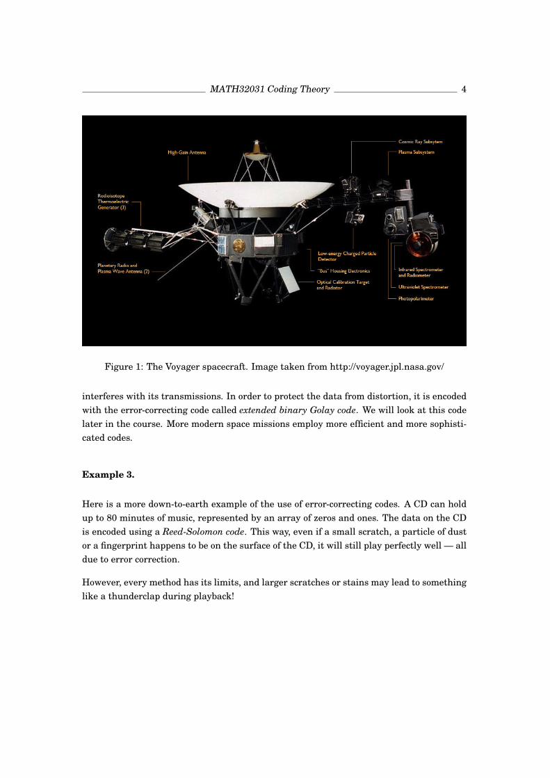
Here is a real-world example of how Coding Theory is used in scientific research.

Voyager 1 is an unmanned spacecraft launched by NASA in 1977. Its primary missionwas to explore Jupiter, Saturn, Uranus and Neptune. Voyager 1 sent a lot of preciousphotographs and data back to Earth. It has recently been in the news because the NASAscientists had concluded that it reached the interstellar space2.

The messages from Voyager 1 have to travel through the vast expanses of interplanetaryspace. Given that the spacecraft is equipped with a mere 23 Watt radio transmitter (pow-ered by a plutonium-238 nuclear battery), it is inevitable that noise, such as cosmic rays,

2See for example the BBC News item dated 12 September 2013 at http://www.bbc.co.uk/news/science-environment-24026153


Figure 1: The Voyager spacecraft. Image taken from http://voyager.jpl.nasa.gov/

interferes with its transmissions. In order to protect the data from distortion, it is encodedwith the error-correcting code called extended binary Golay code. We will look at this codelater in the course. More modern space missions employ more efficient and more sophisti-cated codes.

Example 3.

Here is a more down-to-earth example of the use of error-correcting codes. A CD can holdup to 80 minutes of music, represented by an array of zeros and ones. The data on the CDis encoded using a Reed-Solomon code. This way, even if a small scratch, a particle of dustor a fingerprint happens to be on the surface of the CD, it will still play perfectly well — alldue to error correction.

However, every method has its limits, and larger scratches or stains may lead to somethinglike a thunderclap during playback!


Figure 2: A punch card. Image taken from http://www.columbia.edu/cu/computinghistory

Example 4.

To finish this historical excursion, let us recall one of the very first uses of error-correctingcodes.

In 1948, Richard Hamming was working at the famous Bell Laboratories. Back then, thedata for “computers” was stored on punch cards: pieces of thick paper where holes repre-sented ones and absences of holes represented zeros. Punchers who had to perforate punchcards sometimes made mistakes, which frustrated Hamming.

Hamming was able to come up with a code with the following properties: each codeword is7 bits long, and if one error is made in a codeword (i.e., one bit is changed from 0 to 1 or viceversa), one can still recover the original codeword. This made the punch card technologymore robust, as a punch card with a few mistakes would still be usable. The trade-off,however, was that the length of data was increased by 75%: there are only 16 differentcodewords, therefore, they can be used to convey messages which have the length of 4 bits.

The original Hamming code will be introduced in the course very soon, and every studentwill be expected to learn it by heart!

List of topics

The following topics or notions from pure mathematics will be of use when we will be con-structing error-correcting codes.


• Metric spaces. (We will use the basic terminology from metric spaces. We will defineeverything, so having taken a Metric Spaces course is not a prerequisite.)

• Finite fields, such as Zp. They are finite sets with two operations, + and ×, satisfyingstandard axioms.

• Vector spaces over finite fields. They are finite sets but carry linear structure: notionsof a subspace, a basis, linear independence, etc., will be used.

• Matrices over finite fields, matrix multiplication.

• Polynomials with coefficients in a finite field, their factorisation.


§1. Basic notions

Synopsis. In this lecture, we begin to describe a mathematically rigorous setup for er-ror-detecting an error-correcting codes. We introduce the relevant terminology and define theHamming distance.

Recall the model of information transmission from the first lecture:

senderMESSAGE−−−−−→ encoder

CODEWORD−−−−−−→�� channel

↑NOISE

RECEIVED−−−−−−→WORD

decoderDECODED−−−−−→MESSAGE

user

Let us start defining the terminology we are going to use throughout the course.

Alphabet: a finite set F. We denote by q the number of elements of F: |F| = q, and assumeq > 2.

In this course, F will always be a finite field Fq with q elements. The reason for this isthat we are going to design codes using linear algebra. In particular, q must be a primepower, q = pk. We will mostly work with the field Fp = Z/pZ = {0, 1, 2, . . . ,p − 1} wherep is prime. Note that many books on coding theory allow more general alphabets, such asZ/26Z ∼= {A, . . . ,Z}.

Symbol (or character): an element of the alphabet.

Word: an element of Fn. Note that Fn is the set of all n-tuples of symbols:

Fn = {v = (v1, v2, . . . , vn) | vi ∈ F, 1 6 i 6 n}.

We refer to elements of Fnq as q-ary words of length n. We use the following traditional

terminology: “binary” = “2-ary”, “ternary” = “3-ary”.

Code: a non-empty subset of Fn. We say “q-ary code of length n”. We denote a code by C.That is, C ⊆ Fn, C 6= ∅.

Codeword: an element of the code.

The number of errors in the received word: If a codeword v = (v1, . . . , vn) was trans-mitted and the received word is y = (y1, . . . ,yn), the number of errors in y is the number ofpositions where the character in y differs from the character in v:

d(v,y) = |{i ∈ {1, . . . ,n} : yi 6= vi}|.


Definition (Hamming distance)

If v,y are words of length n, the number d(v,y) defined above is called the Hamming dis-tance between v and y.

Example

Consider the set F32 of binary words of length 3. Explicitly,

F32 = {000, 001, 010, 011, 100, 101, 110, 111}.

Note that d(001, 100) = 2 because in the vectors 001 and 100, the symbols in the first andthe third position differ.

Clearly, if v,y ∈ Fnq , then 0 6 d(v,y) 6 n.

Lemma 1.1 (Properties of the Hamming distance)

For any words v,y, z ∈ Fn,

1. d(v,y) > 0; d(v,y) = 0 ⇐⇒ v = y.

2. d(v,y) = d(y, v).

3. d(v, z) 6 d(v,y) + d(y, z) (the triangle inequality).

Remark: a function d(−,−) of two arguments which satisfies axioms 1.–3. is called a met-ric. This is familiar to those who studied Metric spaces. The Lemma says that the Hammingdistance turns Fn into a metric space.

Proof. Recall that the Hamming distance d(v,y) between two vectors v,y ∈ Fn is the num-ber of positions where these vectors differ.

1. Clearly, the number of positions where v and y differ is an integer between 0 and n. It iszero iff the two vectors are equal.

2. The number of positions in which v differs from y is equal to the number of positions inwhich y differs from v. This is obvious.

3. d(v,y) is the minimal number of symbol changes needed to get from v to y. Take thevector v and make d(v,y) changes to obtain y. Then make d(y, z) changes to obtain z. We


have made d(v,y) + d(y, z) changes to get from v to z. This number of changes may not beminimal (because we may have changed some symbols twice), but it is at least d(v, z).

We continue to define the terminology we are going to use.

Decoder (or decoding scheme, or decoding algorithm): a function DECODE : Fn → C.

Our model of transmission is as follows:

1. A codeword v ∈ C is sent via the channel.

2. A word y is received at the other end. It is possible that y 6= v, because of noise.

3. By looking at y, we want to guess what was v. In other words: we apply the functionDECODE to y.

We always work under assumption that fewer errors during transmission are more likelythan more errors. This motivates the following

Definition (nearest neighbour)

Let C ⊆ Fn be a code. A nearest neighbour of a word y ∈ Fn is a codeword v ∈ C such that

d(v,y) = min{d(z,y) | z ∈ C}.

Notice that a word might have more than one nearest neighbour (there may be severalcodewords at the same distance from y). So a nearest neighbour is not always unique.

Example

Consider the following binary code of length 3: C = {001, 100}. The word 000 ∈ F32 has two

nearest neighbours in C, namely, 001 and 100. Indeed, d(001, 000) = d(000, 100) = 1.

The same can be said of the word 101.

Aside: Interestingly, both 000 and 101 are midpoints between v = 001 and w = 100.Indeed, the distance from 000 to v and w is exactly half the distance between v and w.So, in the metric space Fn defined by the Hamming distance, there can be more than onemidpoint between a pair of points (or there can be none). Note that in a Euclidean space,there is always exactly one midpoint between any two points. This shows that Fn, as ametric space, is quite different from the more conventional Euclidean spaces.


Remark

Let C be a code in Fn.

• If y ∈ Fn is a codeword, then y has unique nearest neighbour in C: namely, y itself.

• We will soon introduce a class of codes called perfect codes. It will turn out that if acode C is perfect, every word in Fn has a unique nearest neighbour in C.

Definition (nearest neighbour decoding)

A decoder for a code C is called nearest neighbour decoding if for any y ∈ Fn, DECODE(y) isa nearest neighbour of y in C.

Throughout the course, a decoder is always a nearest neighbour decoder.

Remark: The above assumption may not determine a decoder completely. Suppose thata received word y has more than one nearest neighbour (which may happen unless thecode is perfect); which one of them will be DECODE(y)? This will depend on a particularimplementation of a decoder.

Nevertheless, the Nearest Neighbour Principle a strong assumption which allows us toprove a number of properties of codes. In particular, it guarantees that if v is a codeword,DECODE(v) = v.

We can now see that transmission can have three possible outcomes. Let v be the code-word which is sent, and let y be the received word.

• DECODE(y) = v. The codeword is decoded correctly.

• y /∈ C (so we know for sure that y contains errors) but DECODE(y) 6= v. The error isdetected but not corrected.

• y ∈ C so that automatically DECODE(y) = y, but y 6= v. This is undetected error.

Intuitively, it is easy to see that to avoid undetected errors, the codewords should be “farapart”, i.e., the distance between any two distinct codewords should be large. That way,a lot of symbol errors in the received word y are needed in order for it to be a codeworddifferent from v — and this is not likely to happen. We will formalise this in the nextlecture.


Synopsis. It turns out that the ability of a code C to detect and correct transmission errorsis expressed by the minimum distance of C, denoted d. We look at simple examples of codesand learn to use the notation (n,M,d)q and [n,k,d]q.

Definition (parameters of a code)

Let C ⊆ Fnq be a code. Then:

• n is the length of the code;

• M denotes the number of codewords, i.e., M = |C|;

• k = logqM is the information dimension of C(warning: k may not be an integer, although we will see that k is an integer for inter-esting types of codes);

• d(C) = min{d(v,w) : v,w ∈ C, v 6= w} is the minimum distance of C. It is defined if|C| > 2.

We say that C is an (n,M,d)q-code or an [n,k,d]q-code.

The importance of the minimum distance d is clear from the following

Theorem 1.2 (The number of errors detected/corrected by a code)

Let C be a code with d(C) = d.

1. A word at a distance 6 d − 1 from a codeword CANNOT be another codeword. We thussay that the code detects up to d− 1 errors.

2. A word at a distance[d−1

2

]from a codeword v has a unique nearest neighbour, which is

v. We say that the code corrects up to[d−1

2

]errors.

Remark: [a] denotes the integer part of a real number a. Thus, [3] = [3.5] = [π] = 3,[7 3

4 ] = 7, etc.

Proof and explanation. Let v ∈ C.

1. If y ∈ Fn and d(v,y) 6 d − 1, then y cannot be another codeword because the minimumdistance from v to another codeword is d.

Thus, if at most d − 1 symbol errors occur in a codeword — i.e., up to d − 1 symbols in the


codeword are changed during transmission via the channel — the received word will not bein the code, and the receiver will know that errors have occurred.

2. Suppose d(v,y) 6 t =[d−1

2

]. If w 6= v is a nearest neighbour of y, then d(y,w) 6 t. Then

d(v,w) 6 d(v,y) + d(y,w) 6 t+ t = 2t 6 d− 1

which contradicts d being the minimum distance of C. Therefore, v is the only nearestneighbour of y.

Thus, if up to t symbol errors occur in a codeword v during transmission, the received wordis decoded back to v by the Nearest Neighbour Decoding principle. This means that theerrors are corrected.

We will now discuss some easy codes and find out how many errors so they detect andcorrect. The following are examples from pre-Hamming era.

Example: the trivial code

Let C = Fn (every word is a codeword).

Then d(C) = 1. Indeed, d(C) is always positive, because it is measured between pairs ofdistinct codewords; and there are codewords at distance 1 in the trivial code, for example000 . . . 0 and 100 . . . 0.

This code C is called the trivial q-ary code of length n. It is an [n,n, 1]q-code. It detects 0errors and corrects 0 errors.

Example: the repetition code

C = {00...0, 11...1, . . . , } ⊂ Fnq has q codewords of length n. Each codeword is made up of one

symbol repeated n times.

The number of codewords is M = q. The q-ary repetition code of length n is an [n, 1,n]q-code.

It detects (n− 1) errors and corrects[n−1

2

]errors.

Is this an efficient error-correcting code? We will be able to answer this question when welearn how to compare codes and see more examples.


To introduce the next example, we need the following

Definition (weight)

The weight, w(v), of a vector v ∈ Fnq is the number of non-zero symbols in v.

Example: the even weight code

The binary even weight code of length n is defined as C = {v ∈ Fn2 : w(v) is even}.

For example, the binary even weight code of length 2 is {00, 11}.

Remark: 0 is an even number! The binary even weight code contains the codeword 00 . . . 0.

Minimum distance: let a binary word v be of even weight. If we change one bit (=binarysymbol) in v, we get a word of odd weight. Indeed, if 0 is changed to 1 or 1 is changed to 0,this increases/decreases the weight by 1, making it odd.

It follows that the distance between two codewords cannot be 1, so d(C) > 2. On the otherhand, d(0000 . . . 0, 1100 . . . 0) = 2. This shows that d(C) = 2.

The code detects 1 error and corrects 0 errors.

The number of codewords: in a codeword v = (x1, x2, . . . , xn), the first n−1 bits (= binarysymbols) can be arbitrary, and then the last one is determined by xn = x1 + x2 + . . . + xn−1,where + is the addition is in the field F2. This makes sure that the weight of the wholecodeword is even. We thus have 2n−1 codewords.

Another argument to that effect is as follows. We can take a binary word and flip (change)its first bit. This operation splits the set Fn

2 into pairs of vectors, such that the vectors in apair only differ in the first bit. Each pair contains one vector of even weight and one vectorof odd weight. Therefore, the number of vectors of even weight is equal to the number ofvectors of odd weight, and is 1

2 |Fn2 | = 2n−1.

Conclusion: this is an [n,n− 1, 2]2-code.

Remark: A widely used code. If an error is detected, the recipient will request retransmis-sion of the codeword where the error occurred. Error correction is not available.


Synopsis. We learn how to compare codes of different length using the code rate, R, andthe relative distance, δ. We plot the simple families of codes on the δ – R plane, but are notsatisfied with the results. We compare Hamming’s approach to codes with Shannon’s andstate Shannon’s Theorem, which shows that codes make it possible to transmit informationover a noisy channel with an arbitrary small probability of error.

Recall that useful propertied of a code C ⊆ Fnq are reflected in its parameters (n,M,d)q,

otherwise written as [n,k,d]q where k = logqM. The power of the code to detect and correcterrors is reflected in its minimum distance, d. There is a special term for codes that sharethe same set of parameters:

Definition (parameter equivalence)

We say that two codes are parameter equivalent, if they both are [n,k,d]q-codes for some n,k, d and q.

Clearly, parameter equivalent codes are of the same value if one considers how efficientthey are in correcting transmission errors3. But how to compare codes of different length?The accepted way in Coding Theory is to use the following two parameters:

Definition (code rate, relative distance)

Let C be an [n,k,d]q-code.

• The code rate of C is R =k

n.

• The relative distance of C is δ =d

n.

We will say that code C ′ is better than code C if R(C ′) > R(C) and δ(C ′) > δ(C).

Remark: Intuitively, it is clear why the higher the code rate, the better. Indeed, whenwe encode information using a code C, we increase the length of information by a factor of1R

. This is easy to see if k is an integer. In this case, we can represent each of the M = qk

messages by a word of length k in the q-ary alphabet. After encoding, it becomes a codewordof length n, so that the length is increased n

k-fold.

It is less clear why we should compare the relative distance of codes. We will not give aformal argument at this stage.

3One of parameter equivalent codes can still be preferable for other reasons — for example, it may be easier towrite a computer programme to encode/decode it.


δ

R

C

C ′

1

1

0

Figure 3: The δ – R plane

The δ – R plane

It is customary to represent a code C by a dot in the R – δ coordinate plane, with coordinatesδ(C) and R(C). See Figure 3.

Looking at Figure 3, we observe that code C ′ is better than code C ′, because the dot repre-senting C ′ is higher and to the right of the dot representing C.

Note that δ and R are not arbitrary real numbers. In fact, they cannot be greater than 1:

Observation (trivial bound). For any code C one has R(C) 6 1. Moreover, R(C) = 1 ifand only if C is a trivial code.

Proof. Let C be an [n,k,d]q-code. Then, by definition, C is a non-empty subset of Fnq . In

particular, 1 6 M = |C| 6 |Fnq | = qn. So 0 6 k = logqM 6 n and 0 6 R = k

n6 1. The

equality is attained only if C = Fnq , i.e., C is a trivial code.

This upper bound on M, k and R is known as the trivial bound, because we use that everycode C is a subset of a trivial code Fn

q .

Observation (0 < δ 6 1). As noted earlier, the Hamming distance between any two wordsof length n is an integer between 0 and n. Therefore, 0 < d(C) 6 n for any code of lengthn, hence 0 < d(C)

n6 1.

It follows that the dots representing codes are all in the 1× 1 square [ 0, 1 ]× [ 0, 1 ].


Discussion: are high δ and high R achievable?

Note that the trivial codes, the repetition codes and the even weight codes are families ofcodes that converge to points on one of the axis in the δ – R plane. That is, one of the limitparemters is zero for each family. This isn’t too satisfactory.

Surely it would be great to have very good codes with both code rate and the relative dis-tance very close to 1. (The code rate cannot equal 1 if we want non-trivial codes.) Thiswould allow us to achieve a very low likelihood of an error when transmitting informationover a noisy channel.

It would be even better to have a family of codes, say C1,C2, . . ., such that the length of Cm

increases and δ(Cm) and R(Cm) both tend to 1. Because a code of fixed length n cannotcorrect more than

[n−1

2

]errors, it is clear that we may never be able to make the likelihood

of an uncorrected error as low as we want. The solution to that is to design a family of codesof increasing length.

Such a “good” family of codes would be represented by a sequence of points converging to(1, 1) in the δ – R plane, like the one shown in Figure 3.

There is only one problem with a “good” family of codes: namely, it does not exist. We willsee why this is so in the next section. At the moment, let us say that not every point ofthe square [ 0, 1 ] × [ 0, 1 ] is attainable — i.e., has a family of codes converging to it. Farfrom that — there is a big region in [ 0, 1 ] × [ 0, 1 ], which contains the upper right cornerof the square and consists of unattainable points. In fact, we’ll see that C ′ in Figure 3 isunattainable. We will start seeing that region when we talk about bounds.

End of discussion.

For the moment, let us plot the simple families of codes on the δ – R plane.

The family of trivial codes: the trivial code of length n is an [n,n, 1]q-code, so δ = 1n

andR = 1.

We can see that this family converges to the point (0, 1) in the δ – R plane.

The family of repetition codes: the parameters of a repetition code are [n, 1,n]q, soδ = 1 and R = 1

n. They converge to the point (1, 0) in the δ – R plane.

The binary even weight codes: they are [n,n − 1, 2]2 codes, represented by ( 2n

, 1 − 1n)

converging to (0, 1).

We plot these families of codes and their limit points in Figure 4.


δ

R

1

1

0

trivial codes

even weight codes

repetition codes

Figure 4: The code families of trivial, repetition and even weight codes

Discussion: Hamming vs. Shannon

We will now talk about the two approaches to codes, both of which date back to 1948. Oneis due to Hamming, the other due to Shannon.

Hamming’s goal was to make sure that all the information is received and decoded correctly.This is possible if we know that the noise is such that there are at most t =

[d−1

2

]symbol

errors per codeword — this is known as the ‘worst case’ assumption. One can rarely makesuch an assumption in practice. Nevertheless, codes designed with this assumption in mindtend to perform well in real-life situations (examples will follow later in the course).

On the other hand, Shannon assumed that the noise in the channel is random. Shannon’smodel of the channel is as follows. The data is sent down the channel, symbol after symbol.There are two possible outcomes when a symbol x is sent down the channel:

• x is received at the other end (no symbol error);

• some other symbol y 6= x is received at the other end (symbol error).

Shannon assumed that symbol errors occur randomly, and the channel is memoryless: thesymbol error in symbol x is independent of errors in all previous symbols.

Shannon stated that the goal of a code must be to maximise

Pcorr = the probability for a codeword to be received and decoded correctly.

He was able to prove his main theorem: even if a channel is noisy, it is still possible to


transmit information with Pcorr arbitrarily close to 1, as long as the code rate R is less thanthe capacity of the channel, and the length n of the code is large.

A simplified statement of Shannon’s theorem is given in the slides below.

Hamming vs. Shannon

Richard Hamming(1915–1998, USA)Founder of Coding Theory

Claude Shannon(1916–2001, USA)Founder of InformationTheory

Hamming’s vs. Shannon’s approach to codes

Noise model ‘Worst case’ Random noiseObjectives Maximise R Maximise R

Maximise d Maximise Pcorr

Who wins inpractical applications? ? ?

Shannon’s Theorem.

Every memoryless channel has a capacity 0 6 Cap 6 1, suchthat for ∀ǫ > 0 and for sufficiently large length n:

① There exists a code with Cap− ǫ < R < Cap andPcorr > 1− ǫ for all codewords;

② Every code with R > Cap+ ǫ contains a codeword for whichPcorr 6 1

2 .


§2. Bounds

Synopsis. To respond to the Information Theory challenge, coding theorists want to designfamilies of codes which have high code rate and high relative distance. There is a trade-offbetween these parameters, which is expressed by inequalities known as bounds. We provetwo such inequalities: the Hamming bound and the Singleton bound. We discuss how theyaffect the shape of the subset of the unit square called “the code region”.

Discussion (not examinable). Shannon’s Theorem set a challenge for coding theorists. Itsaid that for each memoryless channel, there exists a family of codes Ci, with the code rateR(Ci) approaching the capacity Cap of the channel and the probability of correct decodingPcorr(Ci) approaching 1 as i→∞. (Necessarily, the length ni of Ci tends to infinity.)

Shannon’s proof essentially said that for sufficiently large n, one can pick the codewordsrandomly. Provided that the code rate stays below the channel capacity, almost all randomcodes have Pcorr close to 1. This was a fine example of an existence proof ; moreover, the ideaof considering a random object has since found many uses in mathematics.

But random codes are impractical for a number of reasons, such as:

• a randomly picked code is not guaranteed to perform well, it is merely likely to do so— but we might be unlucky;

• to decode a received word, we need to find a codeword closest to it, but for a randomcode this is only possible if we store a complete list of codewords — a lot of storagememory is required.

Coding Theory aims to design more practical families of codes. Ideally, a family of codesshould have high code rate R and high relative distance δ. The latter will ensure that,under reasonable assumptions about the random noise in the channel, Pcorr will go to 1 asn increases.

Intuitively, there is a trade-off between R and d: high R means a large number of code-words, but then the codewords will be more densely packed in the set Fn, and the minimumdistance, hence δ, will be low.

This is expressed rigorously by bounds — inequalities on the parameters of a code.

End of discussion.


Theorem 2.1 (Hamming bound)

For any (n,M,d)q code, M 6 qn∑ti=0(ni

)(q− 1)i

where t = [d−12 ].

Before we prove the theorem, recall that(ni

)is the number of ways to choose i positions

out of n. This integer is called the binomial coefficient. It is given by the formula(ni

)=

n!(n−i)! i! =

n(n−1)...(n−i+1)1·2·...·i .

Definition (Hamming sphere)1

If y ∈ Fn, denoteSt(y) = {v ∈ Fn : d(v,y) 6 t}.

We refer to the set Si(v) as the Hamming sphere with centre v and radius i.

We can find the number of words in the Hamming sphere of radius t as follows:

Lemma 2.2 (the number of points in a Hamming sphere). |St(v)| =

t∑i=0

(n

i

)(q−1)i.

Proof of Lemma 2.2. To get a vector v at distance i from y, we need to choose i positions outof n where y will differ from v. Then we need to change the symbol in each of the i chosenpositions to one of the other q − 1 symbols. The total number of choices for v which is atdistance exactly i from y is thus

(ni

)(q− 1)i.

The Hamming sphere contains all vectors at distance 0 6 i 6 t from v, so we sum in i from0 up to t.

Proof of Theorem 2.1. First of all, we prove that spheres of radius t centred at distinct code-words do not overlap. Suppose for contradiction that v,w ∈ C, v 6= w, and St(v) and St(w)both contain a vector y. Then d(v,w) 6 d(v,y) + d(y,w) 6 t + t = 2t 6 d − 1 whichcontradicts the minimum distance of the code being d.

This means that the whole set Fn contains M disjoint spheres centred at codewords. Eachof theM spheres contains

∑ti=0(ni

)(q−1)i words. The total number of words in the spheres

is M∑t

i=0(ni

)(q− 1)i, and it does not exceed |Fn| = qn. The bound follows.

1A more modern term Hamming ball is also acceptable, and better agrees with the terminology used in MetricSpaces.


Given the length n and the minimum distance d, we may wish to know whether there arecodes with the number of codewords equal to the Hamming bound. Such a code would be themost economical (highest possible number M of codewords, highest rate R = logq(M)/n).Such codes have a special name:

Definition (perfect code)

A code which attains the Hamming bound is called a perfect code.

(“Attains the bound” means that the inequality in the bound becomes an equality for thiscode.)

Back to the above question: we may wish to ask whether there exists a perfect (n,M,d)qcode with given n, d and q.

It turns out that, unfortunately, useful perfect codes are quite rare. We will see theircomplete classification up to parameter equivalence later in the course.

The Singleton bound

Another upper bound on the number M of codewords can be conveniently stated for k =

logqM.

Theorem 2.3 (Singleton bound). For any [n,k,d]q code, k 6 n− d+ 1.

Proof. See the solution to Question 3 on the example sheet, where the bound is establishedby puncturing the code d− 1 times.

Definition (Maximum distance separable code)

A code which attains the Singleton bound is called a maximum distance separable (MDS)code.

A practical question is what do these bounds mean for large n. Let us show, on a graph, theasymptotic form of the Hamming bound and the Singleton bound as n → ∞. We use the δand R coordinates.

Fact (not examinable): Let q = 2. In the limit as n→∞, the Hamming bound becomes the


following inequality:

R 6 1 −H2(δ/2), where H2(p) = p log21p+ (1 − p) log2

11 − p

.

Note that 1 −H2(δ/2) is a smooth decreasing function with value 1 at δ = 0 and value 0 atδ = 1.

Fact: The Singleton bound in terms of δ and R is R = kn6 n−d+1

n= (1 + 1

n) − δ. Taking the

limit as n→∞, we obtainR 6 1 − δ,

independently of q. Let us plot the two asymptotic bounds on the same graph:

0.2 0.4 0.6 0.8 1.0

∆

0.2

0.4

0.6

0.8

1.0

R

We can observe that asymptotically, the Hamming boung is stronger than the Singletonbound. However, this is only true for q = 2. Here is a graph for q = 5, where the limit formof the Hamming bound is different:

0.2 0.4 0.6 0.8 1.0

∆

0.2

0.4

0.6

0.8

1.0

R


The asymptotic form of the two bounds reveal some information about the following set:

Definition (code region)

The q-ary code region is the set of all points (δ,R) in the square [ 0, 1 ] × [ 0, 1 ] such thatthere exists a sequence {Ci}i>1 of q-ary codes, where the length of Ci strictly increases,limi→∞ δ(Ci) = δ and limi→∞ R(Ci) = R.

It follows that the code region lies below both the asymptotic Hamming bound and theasymptotic Singleton bound. It is known, however, that it is strictly less than the setbounded by the two asymptotic bounds. The exact shape of the code region is still an openquestion in Coding Theory.

Important remark: a dot representing an individual code can lie outside the code region.This is because the code region is made up of limits of sequences of codes. For example,trivial codes have R = 1 and as such, are all outside the code region; their limit is the point(0, 1) which is the uppermost point of the code region.


§3. Linear codes

Synopsis. We define the most important class of codes called the linear codes. Their abilityto correct errors is no worse than that of general codes, but linear codes are easier to im-plement in practice and allow us to use algebraic methods. In this lecture, we learn howto define a linear code by its generator matrix and how to find the minimum distance bylooking at weights.

Reminder (vector spaces)

As usual, let Fq denote the field of q elements. Recall that the set Fnq has the structure of a

vector space over the field Fq. If the vectors u, v are in Fnq , we can add the vectors together:

u+ v ∈ Fnq , and multiply a vector by a scalar: λu ∈ Fn

q for all λ ∈ Fq.

The addition and the scalar multiplication are performed componentwise. We will oftenwrite vectors in compact form, as words:

011011, 100110 ∈ F62 7→ 011011 + 100110 = 111101 ∈ F6

2.

Definition (linear code)

A code C ⊂ Fnq is linear, if C is a vector subspace of Fn

q .

Remark: this means that the zero vector 0 belongs to C, and that sums and scalar multi-ples of codewords are again codewords.

Discussion (not examinable). Why are linear codes useful?

• They seem to be as efficient as general codes. In particular, it was proved that Shan-non’s Theorem about the capacity of a channel is still true for linear codes.

• It is possible to define a linear code without specifying all the codewords (see below).

• The minimum distance is easier to calculate than for general codes (see below).

• We can use algebra to design linear codes and to construct efficient encoding anddecoding algorithms.

The absolute majority of codes designed by coding theorists are linear codes. In the rest ofthe course, (almost) all the codes we consider will be linear codes.

End of discussion.


In general, the only way to specify a code C ⊆ Fnq is to list all the codewords of C. But if C

is linear, we can only specify a basis of C. In Coding Theory, this is done in the form of agenerator matrix.

Definition (generator matrix)

Let C ⊆ Fnq be a linear code. A generator matrix of C is a matrix

G =

r1

r2...rk

,

where the row vectors r1, . . . , rk are a basis of C.

Remark (all codewords)

To obtain the list of all codewords of C from the generator matrix G as above, we use that

C = {λ1r1 + . . . + λkrk | λ1, . . . , λk ∈ Fq}.

Because r1, . . . , rk are a basis of C, each codeword is represented by one, and only one, linearcombination λ1r1 + . . . + λkrk.

Note that there are qk such linear combinations: indeed, the first coefficient, λ1, can bechosen from the field Fq in q possible ways, same for λ2, . . . , λk.

Remark

To better visualise the difference between storing all the qk codewords of a linear code andstoring only k rows of a generator matrix, consider the following example. A binary codeof dimension about 1500 was used in computer networks for error detection. While it ispossible to store 1500 rows of a generator matrix, it is definitely not possible to store a listof all 21500 codewords. Indeed, the number 10100 (the googol) is believed to be much biggerthan the number of electrons in the visible Universe; and the googol is less than 2340.

Properties of a generator matrix

Let G be a generator matrix of a q-ary linear code C. Then:


• the rows of G are linearly independent;

• the number n of columns of G is the length of the code;

• the number k of rows of G is the dimension, dim(C), of the code;

• the number of codewords is M = qk;

• the dimension of the code is equal to its information dimension: k = logqM.

In particular, if an [n,k,d]q-code is linear, k is necessarily an integer.

Example

Consider the binary even weight code of length 3:

C = {000, 011, 101, 110}.

We know that the dimension of this code is 2. Therefore, a generator matrix has 2 rows and3 columns.

To write down a generator matrix, we need to take two linearly independent codewords. Wemust not use the zero codeword, 000, because a linearly independent set must not containthe zero vector.

So we can use

G =

[0 1 11 0 1

]or G =

[0 1 11 1 0

]or G =

[1 0 10 1 1

]etc.

Each of these matrices is a generator matrix for C.

Reminder (the weight of a vector)

Let y ∈ Fnq . The weight, w(y), of y is the number of non-zero symbols in y.

Definition (the minimum weight of a code)

The minimum weight of a linear code C is

w(C) = min{w(v) | v ∈ C \ {0}}.

Recall that the minimum distance, d(C), of a code C is a very important parameter whichtells us how many errors can the code detect and correct. The following theorem shows howone can find d(C) if C is linear:


Theorem 3.1. d(C) = w(C) for a linear code C.

Proof. Observe that for v,y ∈ Fnq , d(v,y) = w(v − y). Indeed, d(v,y) is the number of

positions i, 1 6 i 6 n, where vi 6= yi. Obviously, this is the same as the number of positionsi where vi − yi 6= 0. By definition of the weight, this is w(v− y).

Therefore,d(C) = min{w(v− y) | v,y ∈ C, v 6= y}.

Because C is linear, in the above formula v − y ∈ C. Thus, d(C) is the minimum of someweights of non-zero vectors from C, whereas w(C) is the minimum of all such weights. Itfollows that d(C) > w(C).

On the other hand, let z ∈ C \ {0} be such that w(z) = w(C). Recall that 0 ∈ C, so

d(C) 6 d(z, 0) = w(z− 0) = w(z) = w(C).

Hence d(C) 6 w(C). We have proved that d(C) = w(C).

Remark 1. In the proof, we used that C is a linear code at least twice. This condition isessential.

Remark 2. Given a linear code C, one needs to check only M − 1 vectors to computed(C) = w(C). For a non-linear code, one has to check M(M − 1)/2 pairs of vectors tocompute the minimum distance d.

Remark 3. However, if a linear code C is specified by a generator matrix G, it may bedifficult to compute the minimum weight of C. Of course, the minimum weight of C doesnot exceed, but is in general not equal to, the minimum weight of a row of G.


Encoding using a generator matrix

Synopsis. Linear codes are the codes used in virtually all practical applications. In an[n,k,d]q-linear code, messages are all q-ary vectors of length k, and an encoder is a linearmap determined by a generator matrix G of the code. This works especially nicely if G is instandard form. We learn how to find a generator matrix in standard form and look at anexample of encoding.

Let an [n,k,d]q-linear code C be given by a generator matrix

G =

r1

r2...rk

.

As we know, G has k rows and n columns, and the entries of G are in Fq.

Definition (encoder for a linear code)

The generator matrix G gives rise to the encoder for code C, which is the linear map

ENCODE : Fkq → C, ENCODE((u1, . . . ,uk)) = u1r1 + . . . + ukrk,

or, in matrix form,ENCODE(u) = uG ∈ Fn

q .

In this situation, messages are vectors of length k, and the function ENCODE maps messagesto codewords which are of length n. In any non-trivial linear code, n > k, which means thatencoding makes a message longer.

Encoder depends on the choice of a generator matrix. In practice, there is the best choice:

Definition (generator matrix in standard form)

A generator matrix G is in standard form if its leftmost colums form an identity matrix:

G = [Ik |A] =

1 0 . . . 0 ∗ . . . ∗0 1 . . . 0 ∗ . . . ∗

. . .0 0 . . . 1 ∗ . . . ∗

.

Note that the entries in the last n− k columns, denoted by ∗, are arbitrary elements of Fq.


If G is in standard form, then, after encoding, the first k symbols of the codeword show theoriginal message:

u ∈ Fkq 7→ ENCODE(u) = uG = u[Ik |A] = [u |uA]

(note that we started using multiplication of block matrices as explained in Week 01, Ex-amples class).

In this situation, the first k symbols of a codeword are called information digits. The lastn − k symbols are called check digits; their job is to protect the information from noise byincreasing the Hamming distance between codewords.

Theorem 3.2 (generator matrix in standard form)

If a generator matrix in standard form exists for a linear code C, it is unique, and anygenerator matrix can be brought to the standard from by the following operations:

(R1) Permutation of rows.

(R2) Multiplication of a row by a non-zero scalar.

(R3) Adding a scalar multiple of one row to another row.

Proof. Not given — a standard fact from linear algebra. We will do some examples to showhow to find the generator matrix in standard form.

Remark. If we apply a sequence of the row operations (R1), (R2) and (R3) to a generatormatrix of a code C, we again obtain a generator matrix of C. This is implied in the Theorem,and follows from the fact that a basis of a vector space remains a basis under permutations,multiplication of an element of the basis by a scalar, and adding a scalar multiple of anelement to another element. This fact is known from linear algebra.

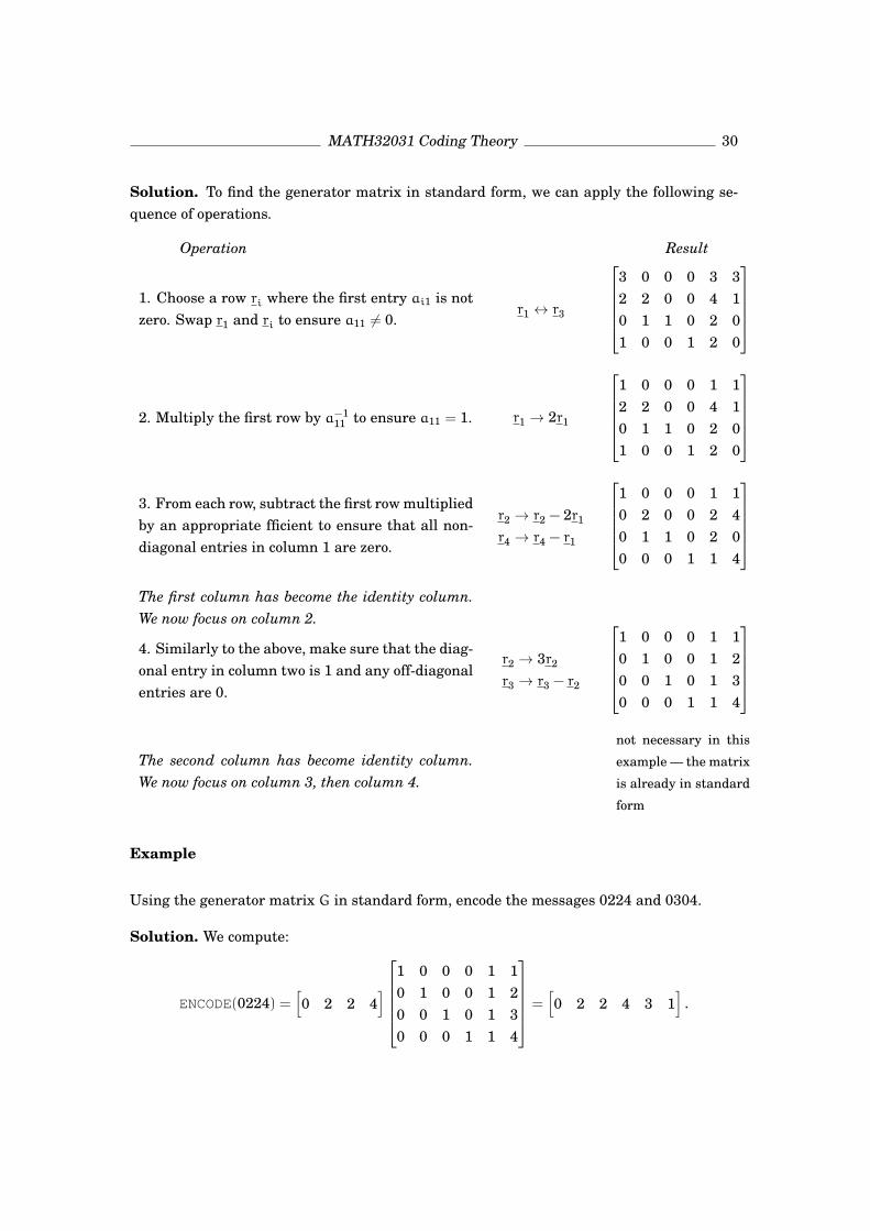
Example (finding a generator matrix in standard form)

A 5-ary code C is given by its generator matrix0 1 1 0 2 02 2 0 0 4 13 0 0 0 3 31 0 0 1 2 0

.

Find a generator matrix G of C in standard form.


Solution. To find the generator matrix in standard form, we can apply the following se-quence of operations.

Operation Result

1. Choose a row ri where the first entry ai1 is notzero. Swap r1 and ri to ensure a11 6= 0.

r1 ↔ r3

3 0 0 0 3 32 2 0 0 4 10 1 1 0 2 01 0 0 1 2 0

2. Multiply the first row by a−111 to ensure a11 = 1. r1 → 2r1

1 0 0 0 1 12 2 0 0 4 10 1 1 0 2 01 0 0 1 2 0

3. From each row, subtract the first row multipliedby an appropriate fficient to ensure that all non-diagonal entries in column 1 are zero.

r2 → r2 − 2r1

r4 → r4 − r1

1 0 0 0 1 10 2 0 0 2 40 1 1 0 2 00 0 0 1 1 4

The first column has become the identity column.We now focus on column 2.

4. Similarly to the above, make sure that the diag-onal entry in column two is 1 and any off-diagonalentries are 0.

r2 → 3r2

r3 → r3 − r2

1 0 0 0 1 10 1 0 0 1 20 0 1 0 1 30 0 0 1 1 4

The second column has become identity column.We now focus on column 3, then column 4.

not necessary in this

example — the matrix

is already in standard

form

Example

Using the generator matrix G in standard form, encode the messages 0224 and 0304.

Solution. We compute:

ENCODE(0224) =[0 2 2 4

]

1 0 0 0 1 10 1 0 0 1 20 0 1 0 1 30 0 0 1 1 4

=[0 2 2 4 3 1

].


Note that in the codeword 022431, the information digits 0224 repeat the original message.The last two symbols, 31, are the check digits. They are found as follows: 0×1+2×1+2×1 + 4× 1 = 3 and 0× 1 + 2× 2 + 2× 3 + 4× 4 = 1. We continue:

ENCODE(0304) =[0 3 0 4

]

1 0 0 0 1 10 1 0 0 1 20 0 1 0 1 30 0 0 1 1 4

=[0 3 0 4 2 2

].

This example illustrates how encoding increases the Hamming distance between messages.One has d(0224, 0304) = 2. However, after encoding, d(022431, 030422) = 4.

In fact, one can check that the code given by this generator matrix has a minimum distanceof 3.

Remark. While not directly relevant to the code and the encoding algorithm, let us pointout that the above messages were created using the following mnemonic key — a pair of5-ary symbols is written as an English letter from A to Y:

00 = A, 01 = B, 02 = C, 03 = D, 04 = E, 10 = F, 11 = G, 12 = H, 13 = I, 14 = J, 20 = K,21 = L, 22 = M, 23 = N, 24 = O, 30 = P, 31 = Q, 32 = R, 33 = S, 34 = T , 40 = U, 41 = V,42 =W, 43 = X, 44 = Y.

The messages 0224 0304 can be read as CODE.

The codewords 022431 030422 are then read as COQ DEM.

Remark (tradeoff between reliability and transmission costs)

The benefit of the increased Hamming distance is that it decreases the likelihood of a trans-mission error. Indeed, one sybmol error in the message 0224 = CO can make it 1224 = HO,and there will be no way to recover the original message.

However, because the code has minimum distance 3, one symbol error in the codeword022431 = COQ will always be corrected by the decoder: 122431 = HOQ will be decoded as022431 = COQ because 122431 is not in the code, and 022431 is the nearest neighbour ofthis vector in the code.

We have to pay for inreased robustness of transmission: if we encode the messages, wehave to transmit 50% more symbols, so that the transmission costs incease.


Synopsis. We have seen how a generator matrix of a linear code is used to encode messagesand produce codewords. We now start discussing decoding. It is a more difficult operationbecause, unlike encoding, it is not given by a linear map. In this lecture we see why cosetleaders are important and construct a standard array of a linear code to find them.

Decoder, error vector

Let C ⊆ Fnq be a linear code. By definition, a decoder for C is a function

DECODE : Fnq → C.

Coding Theory suggests the following model for the transmission of a codeword of a linearcode via a noisy channel:

codeword v ∈ C noise−−−→ y = v+ e,

where

• y ∈ Fnq is the received vector,

• e = y− v is the error vector.

It is assumed that the error vector does not depend on v and is a random vector. Its proba-bilistic distribution depends on the assumptions about the channel.

The job of the decoder is, given y, to estimate the error vector e and then to decode y asy− e.

Even without assuming anything about the channel, we can see that knowing y restrictspossible values of e, as shown in Lemma 3.3.

Definition (coset)

Given a linear code C ⊆ Fnq and a vector y ∈ Fn

q , the set

y+ C = {y+ c | c ∈ C}

is called the coset of y.

Lemma 3.3 (error vector must lie in the coset of received vector)

Any decoder for a linear code C ⊆ Fnq must satisfy DECODE(y) = y − e where e lies in the

coset y+ C of y.


Proof. Let v = DECODE(y). Then v ∈ C and e = y − v. Because C is a linear code, −v ∈ C,therefore e = y+ (−v) ∈ y+ C.

Let us state basic properties of cosets. They are known from Group Theory (see AlgebraicStructures 1). In Group Theory one speaks about left and right cosets. But a linear codeC is a subgroup of the group Fn

q which is abelian. Hence is no difference between left andright cosets, and they are simply called cosets.

Facts about cosets

• C = 0+C is itself a coset. (C is called the trivial coset.) Moreover, C is the coset of anycodeword c ∈ C.

• If y, z ∈ Fnq , then either y+ C = z+ C or (y+ C) ∩ (z+ C) = ∅.

• |y+ C| = |C|.

• There are|Fn

q |

|C|distinct cosets. If n is the length and k is the dimension of C, the

number of cosets isqn

qk= qn−k.

• Thus, the whole space Fnq is split into qn−k disjoint cosets:

Fnq = C t (a1 + C) t . . . t (aqn−k−1 + C).

Nearest Neighbour decoders and coset leaders

Recall that in Coding Theory, we only consider decoders which satisfy the Nearest Neigh-bour Decoding principle. This means that DECODE(y) must be a codeword nearest to y interms of Hamming distance, or one of such codewords. We will now see how this leads tothe following notion:

Definition (coset leader). A coset leader of a coset y + C is a vector of minimum weightin y+ C.

Indeed, let us make the following

Observation. For a linear code,

d(y,DECODE(y)) = d(y,y− e) = w(y− (y− e))

= w(e),


that is, the distance between the received vector and decoded vector is equal to the weightof the error vector.

Conclusion. To decode y, a Nearest Neighbour decoder must estimate the error vector tobe a coset leader of y+ C.

The following construction is a way to find all cosets and coset leaders for a given linearcode C.

The standard array construction

A standard array for a linear code C ⊆ Fnq is a table with |C| = qk columns and qn−k rows.

Each row is a coset. Row 0 is the trivial coset (i.e., C itself). The first column consists ofcoset leaders. The table contains every vector from Fn

q exactly once.

We will show how to construct a standard array, using the linear code C = {0000, 0111,1011, 1100} ⊆ F4

2 as an example.1

Row 0 of the standard array: lists all codewords (vectors in C = 0+C). They must startfrom 0, but otherwise the order is arbitrary.

0000 0111 1011 1100

Row 1: choose a vector a1 of smallest weight not yet listed. Because of its minimum weight,that vector will automatically be a coset leader. Fill in Row 1 by adding a1 to each codewordin Row 0.Say, a1 = 0001. To list its coset, add it to row 0:

0001 0110 1010 1101

Row 2: choose a2 of smallest weight not yet listed, and do the same as for Row 1.Say, a2 = 0010, add it to row 0:

0010 0101 1001 1110

Row 3: same with, say, a3 = 0100:0100 0011 1111 1000

1This code is the even weight code of length 3 with last bit repeated. But the origin of the code is not importantfor the standard array construction.


We obtain the following standard array for the code C = {0000, 0111, 1011, 1100}:

0000 0111 1011 11000001 0110 1010 11010010 0101 1001 11100100 0011 1111 1000

Remarks

1. The coset C = 0 + C always has exactly one coset leader, 0.

2. Other cosets may have more than one coset leader.Exercise: in the above standard array for C, find coset leaders which are not in column 1.

3. Knowing all the coset leaders is not important for decoding. It is enough to know oneleader in each coset — see the next lecture.

Synopsis. For a linear code C, we explicitly describe a Nearest Neighbour decoderDECODE : Fn

q → C based on a standard array for C. For binary C sent via a binary symmetricchannel, we find the probability Pundetect of an undetected transmission error. It is related tothe weight distribution function of C.

The Standard Array decoding

Let C ⊆ Fnq be a linear code. In the previous lecture, we proved that any Nearest Neighbour

decoding algorithm for C must satisfy

DECODE(y) = y− COSET LEADER(y+ C).

This suggests the following decoding algorithm for C:

Algorithm 3.4 (the standard array decoder)

Preparation. Construct a standard array for C.

Decoding.

• Receive a vector y ∈ Fnq .

• Look up y in the standard array:

– The row of y starts with its chosen coset leader ai.


– The column of y starts with y− ai.

• Return the topmost vector of the column of y as DECODE(y).

Example

Using the standard array decoder for the binary code C = {0000, 0111, 1011, 1100},

• decode the received vectors 0011 and 1100;

• give an example of one bit error occurring in a codeword and being corrected;

• give an example of one bit error occurring in a codeword and not being corrected.

Solution. We already know a standard array for C:

0000 0111 1011 11000001 0110 1010 11010010 0101 1001 11100100 0011 1111 1000

The received vector 0011 is in the second column, so DECODE(0011) = 0111. The receivedvector 1100 is a codeword (in the fourth column), so DECODE(1100) = 1100.

Suppose that the codeword 0000 is sent. If an error occurs in the last bit, the word 0001 isreceived and decoded correctly as 0000. If an error occurs in the first bit, the word 1000 isreceived and decoded incorrectly as 1100.

Remark (a standard array decoder is not unique)

Recall that there may be more than one possible standard array for the code C. Indeed, inthe above example the coset 0100+C has two coset leaders: 0100 and 1000. Thus, we couldconstruct a different standard array for C:

0000 0111 1011 11000001 0110 1010 11010010 0101 1001 11101000 1111 0011 0100

The decoder associated to this standard array is different from the decoder consideredabove. Both decoders decode the same linear code C and both are Nearest Neighbour de-coders. A linear code can have more than one Nearest Neighbour decoder.

However, if C is a perfect linear code, then


• each coset has only one coset leader, so the Standard Array decoder is unique;

• each vector has a unique nearest neighbour in C; thus, there is only one NearestNeighbour decoder, namely the Standard Array decoder.

The above facts about perfect codes are true by questions 8(b) and 13(c) on the examplesheets.

Reminder (the number of errors corrected by a code)

Recall that a code with minimum distance d corrects t =[d−1

2

]errors.

The code C in the above example is linear, hence d(C) = w(C) = 2 (it is easy to find theminimum weight of the code by inspection). This means that the code corrects

[ 2−12

]= 0

errors. And indeed, as we saw in the example, it is possible that one bit error occurs in acodeword and is not corrected.

So, from the point of view of Hamming’s theory, this code C has no error-correcting capabil-ity. (It still detects one error.)

But in Shannon’s theory, error-detecting and error-correcting performance of a code aremeasured probabilistically.

Error-detecting and error-correcting performance of a linear code:Shannon’s theory point of view

Shannon’s Information Theory is interested in how likely is it that a transmission error ina codeword is not detected/corrected by a decoder of C.

We will answer these questions for a binary linear code C, but we need to have a stochasticmodel of the noise. Here it is:

Assumption. The channel is BSC(r), the binary symmetric channel with bit error rate r.

This means that one bit (0 or 1), transmitted via the channel, arrives unchanged withprobability 1 − r, and gets flipped with probability r:


0

1

1 − r

r

r

1 − r

0

1

When a codeword v is transmitted, the channel generates a random error vector and addsit to v. By definition of BSC(r), for a given e ∈ Fn

2 one has

P(the error vector equals e) = ri(1 − r)n−i, where i = w(e)

(similar to Q4(b) on the Example sheet).

Recall that an undetected error means that the received vector v+e is a codeword not equalto v. Note that, if v ∈ C and C is a vector space,

v+ e ∈ C ⇐⇒ e ∈ C.

Therefore, an undetected error means that the error vector is a non-zero codeword. We cannow calculate

Pundetect = P(undetected error) =∑e∈C,e 6=0

P(the error vector is e)

=

n∑i=1

Airi(1 − r)n−i,

where

Ai is the number of codewords of weight i in C.

The coefficients Ai give rise to the following useful function:

Definition (the weight distribution function)

Let C ⊆ Fnq be a linear code. The weight distribution function of C is the polynomial A(x) =

A0 +A1x+A2x2 + . . . +Anx

n. It is otherwise written as

A(x) =∑v∈C

xw(v).


Lemma 3.5 (Pundetect via the weight distribution function)

Suppose that a binary linear code C of length n with weight distribution function A(x)

is transmitted via BSC(r). Then the probability of an undetected transmission error isPundetect = (1 − r)n

(A( r

1−r) − 1

).

Proof (not given in class, not examinable). One has A0 = 1 because a linear code C containsexactly one codeword of weight 0, namely 0. Therefore A(x) − 1 = A1x+A2x

2 + . . . +Anxn,

which gives A( r1−r

) − 1 = A1r

1−r+ A2

r2

(1−r)2 + . . . + Anrn

(1−r)n . Multiplying the right-handside by (1 − r)n, one obtains the formula for Pundetect deduced earlier.

Example

For the binary code C = {0000, 0111, 1011, 1100} as above, the weight distribution functionis

A(x) = 1 + x2 + 2x3,

because C has one codeword of weight 0, zero codewords of weight 1, one codeword of weight2 and two codewords of weight 3. If a codeword of C is transmitted via BSC(r), then anundetected error occurs with probability Pundetect = r

2(1 − r)2 + 2r3(1 − r).

Remark

In an earlier example we sent the codeword 0000 of the code C down the channel andreceived the vector 1000. In this case, the error was detected (because the received vectorwas not a codeword), but not corrected.

In the next lecture, we will find the probability of an error being corrected for C.


Error-correcting performance of a linear code

Synopsis. As in the previous lecture, we assume that a binary linear code C is transmittedvia BSC(r). We find Pcorr, the probability that a codeword is decoded correctly, in terms ofweights of coset leaders of C. We conclude by stating the need for better codes and betterdecoding algorithms.

Let C be a binary linear code. A codeword v ∈ C is transmitted via the binary symmetricchannel with bit error rate r, and a vector v + e is received and decoded. We say that the vis decoded correctly if DECODE(v+ e) = v. We denote

Pcorr(C) = P(v is decoded correctly).

If we use a Standard Array decoder,

DECODE(v+ e) = v+ e− COSET LEADER(v+ e)

= v+ e− COSET LEADER(e).

Therefore, correct decoding occurs whenever the error vector is a coset leader in the standardarray.

Recall that e equals a given coset leader of weight i with probability ri(1− r)n−i. We obtain

Lemma 3.6 (formula for Pcorr)

For a binary linear code C, let αi be the number of cosets where the coset leader is ofweight i. Then

Pcorr(C) =

n∑i=0

αiri(1 − r)n−i.

Example

Recall the code with a standard array

0000 0111 1011 11000001 0110 1010 11010010 0101 1001 11101000 1111 0011 0100

One has α0 = 1, α1 = 3, α2 = α3 = 0, so Pcorr(C) = (1 − r)4 + 3r(1 − r)3.


Numerical example

Let r = 0.1 be the bit error rate of the channel1. Let us compare two scenarios:

1. a two-bit message is transmitted via the channel without any encoding;

2. a two-bit message is encoded using the code C as above, then the codeword of length4 is transmitted via the channel, and decoded at the other end.

In each case, we determine the probability that the message arrives uncorrupted.

Case 1: by definition of BSC(0.1), the probability of no errors in a message of length 2 is(1 − 0.1)2 = 0.81.

Case 2: by the above calculation, the probability of correct decoding is Pcorr(C) = (1−0.1)4+

3× 0.1(1 − 0.1)3 = 0.8748.

As we can see, the code C allows us to improve the reliability of transmission, but not bymuch (the error probability goes down from 0.19 to about 0.12, i.e., is not even halved). Themain reason for that is that C is not a good code. From Hamming’s theory perspective, itdoes not correct even a single error.

Discussion: how can one improve performance of error-correcting codes?

1. One can use longer codes (increase n).

However, decoding is going to be a problem. We described the standard array decodingalgorithm for linear codes. Its main disadvantage is the storage requirement: the standardarray contains all vectors of length n and must be stored in memory while the decoderoperates. This requires an amount of memory proportional to nqn.

Example: The Voyager 1 and 2 deep space missions used a binary codeof length 24 to transmit colour photographs of Jupiter and Saturn back toEarth in 1979–81. A standard array decoder for this code would require24× 224 bits of memory, which is 48 Mbytes.

This is little by today’s standards, however, the Voyager 1 spacecraft hasrecently left the Solar system with 68 kbytes of onboard memory...

1This is a very bad channel. When telephone lines were first used for transmission of binary data, the bit errorrate was of the order 10−3.


In the next section, we will introduce an improved technique called syndrome decoding.It will require significantly less memory, but decoding a received vector will require morecomputation. Syndrome decoding is based on the notion of a dual linear code.

2. One can use codes which correct more errors.

In the rest of the course, we will construct several families of codes algebraically.

End of discussion.


§4. Dual codes

Synopsis. We define the dual code C⊥ of a linear code C. If C has a generator matrix instandard form, we learn how to find a generator matrix of C⊥.

Definition (inner product)

For u, v ∈ Fnq , the scalar (element of Fq) defined as

u · v =n∑

i=1

uivi

is called the inner product of the vectors u and v.

Properties of the inner product

(1) u · v = uvT (matrix multiplication).

Explanation: we write elements of Fnq as row vectors. Thus, u is a row vector (u1, . . . ,un),

and vT is the transpose of v, so a column vector

v1

v2...vn

. Multiplying u and vT as matrices

(an 1× n matrix by an n× 1 matrix), we obtain a 1× 1 matrix, i.e., a scalar in Fq.

(2) u · v = v · u (symmetry).

Explanation: is easily seen from the definition.

(3) For a scalar λ ∈ Fq we have (u + λw) · v = u · v + λ(w · v); u · (v + λw) = u · v + λ(u ·w)(this property is known as bilinearity).

Explanation: we know that the matrix product in uvT is bilinear.

Definition (dual code)

Given a linear code C ⊆ Fnq , we define the dual code C⊥ as

C⊥ = {v ∈ Fnq | v · c = 0 for every c ∈ C}.


Example (the dual code of the binary repetition code)

Let Repn = {00 . . . 0, 11 . . . 1} ⊆ Fn2 be the binary repetition code of length n.

By definition, (Repn)⊥ = {v ∈ Fn

2 | v · 00 . . . 0 = 0, v · 11 . . . 1 = 0}. The first condition,v · 00 . . . 0 = 0 is vacuous (holds for all vectors v ∈ Fn

2 ). The second condition, v · 11 . . . 1,means v1 + v2 + . . . + vn = 0 in F2, i.e., v ∈ En, the binary even weight code of length n.Thus, (Repn)

⊥ = En.

Lemma 4.1

Let A be an m× n matrix over Fq. The following are equivalent:

i. A = 0 (zero matrix);ii. ∀u ∈ Fm

q uA = 0;iii. ∀v ∈ Fn

q AvT = 0;iv. ∀u ∈ Fm

q ∀v ∈ Fnq uAvT = 0.

Remark: 0 denotes the column vector

0...0

= (0, . . . , 0)T = 0T .

Proof (not given in class — easy exercise). Obviously, i. =⇒ ii. =⇒ iv.

Now, take u = (0, . . . , 1, . . . , 0) (the ith component is 1, the rest are 0) and v = (0, . . . , 1, . . . , 0)(the jth component is 1, the rest are 0), and observe that uAvT = aij, the (i, j)-th entry ofA. Therefore, iv. =⇒ i., and i. ⇐⇒ ii. ⇐⇒ iv.

In the same way, i. ⇐⇒ iii. ⇐⇒ iv.

Proposition 4.2. If G is a generator matrix for C, then C⊥ = {v ∈ Fnq | vGT = 0}.

Proof. Recall thatC = {uG : u ∈ Fk

q}

(see Encoding using a generator matrix in §3). Hence

C⊥ = {v ∈ Fnq : ∀u ∈ Fk

q v · (uG) = 0} = {v ∈ Fnq : ∀u ∈ Fk

q vGTuT = 0}.

where we use the rule (AB)T = BTAT for matrix multiplication. By Lemma 4.1(iii. =⇒ i.),this is {v : vGT = 0}.


Corollary 4.3. C⊥ is a linear code. (By Question 12 on the example sheets.)

Theorem 4.4

Assume that C has a k × n generator matrix G = [ Ik |A ] in standard form. Then C⊥ hasgenerator matrix

H = [−AT | In−k ].

Proof. Notation: if v ∈ Fnq , we will write v = [ x |y ] where x ∈ Fk

q and y ∈ Fn−kq . Here x

denotes the vector formed by the first k symbols in v, and y denotes the vector formed bythe last n− k symbosl in v.

Observe that A is a k × (n − k) matrix, so its transpose AT is an (n − k) × k matrix, henceH is an (n− k)× n matrix. The last n− k columns of H are identity columns, therefore therows of H are linearly independent. So H is a generator matrix of the linear code

{yH : y ∈ Fn−kq } = { [ −yAT |y ] : y ∈ Fn−k

q }

= { [ x |y ] : y ∈ Fn−kq , x+ yAT = 0 }

= { [ x |y ] : [ x |y ]

Ik

−−−

AT

= 0 }

= { [ x |y ] : [ x |y ]GT = 0 }

= C⊥ by Proposition 4.2.

Synopsis. We prove an important theorem about the properties of a dual code C⊥. Weintroduce a new decoding algorithm for linear codes called syndrome decoding. It requiresthe knowledge of a check matrix of the code.

Definition (check matrix)

A check matrix for a linear code C means a generator matrix for C⊥.

If C is a binary code, we can also say parity check matrix.(The reason for this terminology will be explained soon.)

Question: what if the code C does not have a generator matrix G in standard form?


Answer: for practical purposes, we will replace C by a linearly equivalent code with G instandard form.

Definition (linearly equivalent codes)

Two linear codes C,C ′ ⊆ Fnq are linearly equivalent, if C ′ can be obtained from C by a

sequence of linear transformations of the following types:

(C1) choose indices i, j; in every codeword, swap symbols xi and xj;

(C2) choose index i and non-zero λ ∈ Fq; in every codeword, multiply xi by λ.

Exercise: linearly equivalent codes are parameter equivalent. Indeed, transformations(C1), (C2) do not change:

• the dimension, dimC, of the code;

• the weight, w(C), of the code.1

Fact from linear algebra

Every generator matrix can be brought into the standard form by using row operations(R1), (R2), (R3) from §3 and column operations (C1). We can thus find a generator matrixin standard form for a linearly equivalent code.

Theorem 4.5

If C ⊆ Fnq is a linear code of dimension k, then:

i. dimC⊥ = n− k;

ii. (C⊥)⊥ = C;

iii. if H is a check matrix for C, then C = {v ∈ Fnq : vHT = 0}.

Proof. i. (sketch of proof ) If C has a generator matrix in standard form, then Theorem4.4 yields a generator matrix for C⊥ with n − k rows, so we are done. Otherwise, usingoperations (C1), permute symbol positions in C and obtain a code C ′, linearly equivalent

1The weight of C is the same as the minimum weight of C — the minimum weight of a non-zero codeword.


to C, with a generator matrix in standard form. One has dim(C ′)⊥ = n − k. Now observethat the same permutation applied to C⊥ gives (C ′)⊥, so dimC⊥ = dim(C ′)⊥ = n− k.

ii. c ∈ C =⇒ ∀v ∈ C⊥ v · c = c · v = 0 =⇒ c ∈ (C⊥)⊥. This shows that C ⊆ (C⊥)⊥. Butdim(C⊥)⊥ = n− (n− k) = k = dimC. So C = (C⊥)⊥.

iii. is immediate by ii. and Proposition 4.2.

Remark

Thus, a check matrix H allows us to check whether a given vector v ∈ Fnq is a codeword in

C: this is true iff vHT = 0.

Definition (syndrome)

Let H be a check matrix for a linear code C ⊆ Fnq . Let y ∈ Fn

q . The vector

S(y) = yHT

is called the syndrome of y. The linear map

S : Fnq → Fn−k

q

is the syndrome map.

We can see that the syndrome map can be used for error detection:

S(y) = 0 ⇐⇒ y is a codeword.

We will now use the syndromes in error correction. Using the above notation:

Theorem 4.6. S(y) = S(v) ⇐⇒ y, v are in the same coset of C.

Proof. yHT = vHT ⇐⇒ (y − v)HT = 0 ⇐⇒ y − v ∈ C. By definition of cosets, this meansthat v is in the coset of y.

Syndrome decoding

If we know a check matrix H for a linear code C ⊆ Fnq , we can improve the standard array

decoder for C. We will write the same decoder differently; it will require much less memorybut more calculations.


Algorithm 4.7 (the syndrome decoder)

Preparation. Construct a table of syndromes, with qn−k rows, of the form

Coset leader ai S(ai)

The top row contains the codeword 0 and its syndrome S(0) = 0.

At each step, choose a vector ai ∈ Fnq of smallest weight such that S(ai) does not appear in

the table; then ai is a coset leader of a new coset.

Decoding.

• Receive a vector y ∈ Fnq .

• Calculate S(y) = yHT .

• In the table, find ai with S(ai) = S(y). Then ai is the coset leader of the coset of y.

• Return DECODE(y) = y− ai.

Remarks

The syndrome decoder is based on a choice of one coset leader in every coset. This is thesame as for the standard array decoder.

In fact, if the same coset leaders are chosen in both decoders, both decoders with yield thesame function DECODE : Fn

q → C. They differ only in the way this function is computed.

The number of arithmetic operations required to calculate the syndrome S(y) = yHT canbe of order n2, whereas the standard array decoder requires ∼ n operations to look up avector. On the other hand, the amount of memory required by the syndrome decoder isproportional to qn−k which is better thatn qn for the standard array, especially for codeswith high code rate k

n.

Example of syndrome decoding

This example was given in the examples class.

Let C be the binary linear code with generator matrix

[1 0 0 1 1 00 0 1 0 1 1

].


(a) Find a codeD linearly equivalent to C such thatD has a generator matrix in standardform.

(b) Find a parity check matrix H for the code D.

(c) Construct the table of syndromes for D using the matrix H.

(d) Using the table of syndromes, decode the received vector y = 111111.

Solution. (a) Swap columns 2 and 3 to obtain a generator matrix G =

[1 0 0 1 1 00 1 0 0 1 1

]in standard form. Let D be the code generated by this matrix.

We now forget about the code C and work only with D.

(b) We can find H using Theorem 4.4. Observe that G = [ I2 |A ] with A =

[0 1 1 00 0 1 1

].

Put H =

0 0 1 0 0 01 0 0 1 0 01 1 0 0 1 00 1 0 0 0 1

.

(c) When calculating syndromes, it is useful to observe that the syndrome of a vector0 . . . 010 . . . 0 (with 1 in position i and 0s elsewhere) is equal to the ith column of H, trans-posed.

The syndrome map is linear, so the syndrome of a sum of two vectors is the sum of theirsyndromes, etc.

For example, S(011000) = 0011+1000 = 1011 (the sum of the second and the third columnsof H, transposed).

vector syndrome leader?000000 0000 yes000001 0001 yes000010 0010 yes000100 0100 yes001000 1000 yes010000 0011 yes100000 0110 yes

All vectors of weight 1 have different syndromes, so they all are coset leaders. We needmore coset leaders, hence we start looking at vectors of weight 2, then weight 3:


000011 0011 no, syndrome already in the table000101 0101 yes001001 1001 yes001010 1010 yes001100 1100 yes010100 0111 yes011000 1011 yes101000 1110 yes001101 1101 yes011100 1111 yes

When we try a vector, say of weight 2, and find that is syndrome is already in the table, weignore that vector and try another one.

We found 16 = 26−2 coset leaders so we stop.

(d) S(111111) = 1010 which is the syndrome of the coset leader 001010 in the table. There-fore, DECODE(111111) = 111111 − 001010 = 110101.

(Sanity check. The decoded vector must be a codeword. Indeed, we can see that the vector110101 is the sum of the two rows of the generator matrix for D.)

End of example.


§5. Hamming codes

Synopsis. Hamming codes are essentially the first non-trivial family of codes that we shallmeet. We start by proving the Distance Theorem for linear codes — we will need it to de-termine the minimum distance of a Hamming code. We then give a construction of a q-aryHamming code.

We already know how to read the length and the dimension of a linear code C off a checkmatrix H of C:

• the number of columns of H is the length of C;

• the number of columns minus the number of rows of H is the dimension of C.

The following theorem tells us how to determine the minimum distance of C using H.

Theorem 5.1 (Distance Theorem for Linear Codes)

Let C ⊆ Fnq be a linear code with check matrix H. Then d(C) = d if and only if every set

of d − 1 columns of H is linearly independent and some set of d columns of H is linearlydependent.

Proof. By Theorem 4.5, a vector x = (x1, . . . , xn) ∈ Fnq is a codeword if and only if xHT = 0.

This can be written asx1h1 + x2h2 + . . . + xnhn = 0

where h1, . . . ,hn are the columns of the matrix H. The number of columns of H that appearin the linear dependency x1h1 + . . . + xnhn = 0 with non-zero coefficient is the weight of x.Therefore, d(C), which is the minimum possible weight of a non-zero codeword of C, is thesmallest possible number of columns of H that form a linear dependency.

Example

Use the Distance Theorem to find the minimum distance of the ternary linear code with

check matrix H =

[1 1 1 01 2 0 1

].

Solution. Step 1. Note that H has no zero columns. This means that every set of 1 columnis linearly independent (a one-element set is linearly dependent iff that element is zero).So d > 2.


Step 2. Any two columns of H are linearly independent, because no two columns are pro-portional to each other. So d > 3.

Step 3. There are three linearly dependent columns in H: for example, columns 1, 3 and 4

form a linear dependency

[11

]−

[10

]−

[01

]= 0. Therefore, d = 3.

Remark: although, for small matrices, the algorithm for finding d can be used in practice,it requires a lot of computations for large n. Essentially, one needs to check all possible setsof columns of H for linear dependence. The required number of operations is exponentialin n.

The projective space Pn−1(Fq)

Definition (line, representative vector, projective space)

A line is a 1-dimensional subspace of the vector space Fnq .

A representative vector of a line is a non-zero vector u from that line. The line is then givenby {λu | λ ∈ Fq}.

The projective space Pn−1(Fq) is the set of all lines in Fnq .

Remark: the terminology comes from euclidean geometry — in the euclidean plane, the setof all vectors proportional to a given non-zero vector is a straight line through the origin.Moreover, projective spaces over the field R of real numbers are well-studied geometricobjects.

For example, P1(R) — the set of all lines through the origin in the euclidean plane — canbe thought of as the unit circle with antipodes identified. We are working over a finite fieldFq where these notions are less intuitive.

Definition (Hamming codes)

Let s > 2 be given. We let Ham(s,q) denote an Fq-linear code whose check matrix hascolumns which are representatives of the lines in Ps−1(Fq), exactly one representative vec-tor from each line.


Remark

Ham(s,q) is defined up to a linear equivalence:

• we can multiply a column by a non-zero scalar to get another representative of thesame line;

• we can put columns in any order.

This means that Ham(s,q) is not just one code but a class of linearly equivalent codes. Wewill therefore say “a Ham(s,q) code” to mean any of the linearly equivalent codes.

For convenience, we may make the last s columns the identity columns, to get a checkmatrix H in standard form.

Example: Ham(3, 2)

To construct a parity check matrix for Ham(3, 2), we need to take one non-zero column fromeach line in F3

2. Note that for binary vectors, a line λu | λ ∈ F2} consists only of two points,0 and u. Therefore, Ps−1(F2) is the same as the set of all non-zero column binary vectors ofsize s.

We start filling in the parity check matrix by putting the identity columns at the end. Wedo this to obtain a parity check matrix in standard form.

We can find a total of 7 non-zero binary vectors of size 3:

H =

1 1 1 0 1 0 01 1 0 1 0 1 01 0 1 1 0 0 1

From this parity check matrix in standard form, we can reconstruct the generating matrix:

G =

1 0 0 0 1 1 10 1 0 0 1 1 00 0 1 0 1 0 10 0 0 1 0 1 1

This is, up to linear equivalence, the generating matrix of the original [7, 4, 3]2 code in-vented by Hamming.


A historical remark

Despite their name, the q-ary Hamming codes were not invented by Hamming. RichardHamming told Claude Shannon (who he shared an office with at Bell Labs) about his binary[7, 4, 3]-code, and Shannon mentioned it in his paper of 1948. That paper was read byMarcel J. E. Golay (1902–1989), a Swiss-born American mathematician and electronicsengineer, who then suggested the Ham(s,q) construction in his paper published in 1949.Golay went further and constructed two perfect codes which are not Hamming codes. Heasked whether there are any more perfect codes.

We will see the Golay codes, and will learn the answer to Golay’s question about perfectcodes, later in the course.

Synopsis. By calculating the parameters of a Ham(s,q) code explicitly, we prove that Ham-ming codes are a family of perfect codes with minimum distance 3. We show that syndromedecoding works for Hamming codes in an especially simple way.

We considered an example of a Ham(3, 2) code, which — by looking at its generator matrix— turns out to be a [7, 4,d]2 code. It is not difficult to see that d = 3, see Question 10 on theexample sheets. We know that any [7, 4, 3]2-code is perfect, see Question 5 on the examplesheets.

We will now generalise this and show that all Hamming codes are perfect.

Theorem 5.2 (properties of Hamming codes)

Ham(s,q) is a perfect [n,k,d]q code where

n =qs − 1q− 1

, k = n− s, d = 3.

Proof. The length n of the code is equal to the number of columns in the check matrix,which is |Ps−1(Fq)|, the number of lines in Fs

q.

Observe that two lines intersect only at one point, namely 0. The set Fsq \ {0} is therefore a

disjoint union of lines. Each line {λu : λ ∈ F} contains q− 1 non-zero points.

So the number of lines in Fsq can be found as

|Fsq \ {0} |q− 1

=qs − 1q− 1

.

Note that k = dim Ham(s,q) = n − s because by construction, the check matrix H has srows.


To find the minimum distance, we use the Distance Theorem for linear codes. Note thatany two columns of H are linearly independent because they are from different lines inFsq. (Two vectors can be linearly dependent only if they are proportional to each other, i.e.,

belong to the same line.) Therefore, d > 3.

On the other hand, H has columns (a, 0, 0, . . . , 0)T , (0,b, 0, . . . , 0)T and (c, c, 0, . . . , 0)T , fromthree different lines, linearly dependent:

a−1

a

0...0

+ b−1

0b...0

− c−1

c

c...0

= 0.

So d = 3 by the Distance Theorem.

It remains to show that Ham(s,q) is perfect. We compute the Hamming bound: put t =

[(d − 1)/2] = [2/2] = 1 and calculateqn∑t

i=0(ni

)(q− 1)i

=qn(

n0

)+(n1

)(q− 1)

, where(n0

)+(

n1

)(q − 1) = 1 + n(q − 1) = 1 +

qs − 1q− 1

(q − 1) = qs. So the Hamming bound equals

qn−s = qk =M (the number of codewords). Thus, Ham(s,q) is perfect.

Remark: n =qs − 1q− 1

= qs−1+qs−2+ . . .+q+1. The right-hand side is obviously an integer.

Syndrome decoding for Ham(s,q)

By Question 13 on the example sheets, the coset leaders of Ham(s,q) are the vector 0 andall the vectors of weight 1.

Syndromes of coset leaders: let a = (0, . . . , 0, λ, 0, . . . , 0) be a coset leader, where λ is inposition i. Then the syndrome of a is S(a) = aHT = λ× [ the ith column of H ]T .

Reminder about the syndrome decoding: DECODE(y) = y − a where a is a coset leader withS(a) = S(y).

Hence we obtain the following

Decoding procedure for a Hamming code:

Let a Hamming code be given by its check matrix H.


Suppose that a vector y is received.

• Calculate S(y) = yHT .

• Find a column of H such that S(y) = λ × that column. (ith column)

• Subtract λ from the ith position in y. The result is the codeword DECODE(y).

See the answer to Question 17 on the example sheets for an example.


§6. Cyclic codes

Cyclic codes are an interesting class of linear codes discovered in 1957.

Definition (cyclic code)

A cyclic code in Fnq is a linear code C such that

(a0,a1, . . . ,an−1) ∈ C =⇒ (an−1,a0, . . . ,an−2) ∈ C.

Remark: the vector (an−1,a0, . . . ,an−2) is called the cyclic shift of (a0, . . . ,an−1).

We can iterate the cyclic shift, so if (a0,a1, . . . ,an−1) is a codeword of a cyclic code C, then(an−2,an−1,a0, . . . ,an−3) is a codeword, ..., (a1, . . . ,an−1,a0) is a codeword.

To study cyclic codes, we need certain algebraic methods which go beyond the basic linearalgebra. We need to work with commutative rings.

Definition (commutative ring)

A commutative ring is a set R equipped with two binary operations, + (addition) and ×(multiplication), which satisfy the eight standard axioms.

Remark: for reference, the axioms of a commutative ring are as follows. For all a,b, c ∈ R(writing ab for a · b):

1. (a+ b) + c = a+ (b+ c);2. a+ b = b+ a;3. ∃0 ∈ F: a+ 0 = a;4. ∀a ∈ F ∃− a ∈ F: a+ (−a) = 0;5. (ab)c = a(bc);6. ab = ba;7. ∃1 ∈ F: 1 6= 0, a · 1 = a;8. a(b+ c) = ab+ ac.

Note that the axiom “∀a ∈ R \ {0} ∃a−1 ∈ R: aa−1 = 1” is not part of the axioms of acommutative ring. Commutative rings which satisfy this additional axiom (the inverseaxiom) are fields; see the examples class in Week 1.

Note that the word “commutative” refers to the commutativity of multiplication, ab = ba.


Example: the ring of polynomials

We will consider Fq[x], the ring of polynomials with coefficients in the field Fq. As a set,

Fq[x] = {a0 + a1x+ . . . + anxn | n > 0,a0,a1, . . . ,an ∈ Fq},

with addition and multiplication defined for polynomials in the standard way.

Note that Fq[x] is an infinite ring, though Fq is a finite field.

If f = a0 + a1x + . . . + anxn is a polynomial, an 6= 0, we say that the degree of f is n andwrite deg f = n. Every non-zero polynomial has a degree.

Synopsis. We would like to study cyclic codes using an algebraic structure which is richerthan just a vector space. An appropriate structure is a ring. But the ring Fq[x] of polynomialsis too big (infinite). New, smaller rings can be produced using the quotient ring construction.In particular, cyclic codes coincide with ideals of the ring Rn = Fq[x]/(x

n − 1).

We are going to define quotient rings. An essential ingredient of that construction is anideal.

Definition (ideal)

An ideal of a commutative ring R is a subset I ⊆ R satisfying three conditions:

(1) 0 ∈ I; (2) x,y ∈ I =⇒ x+ y ∈ I; (3) r ∈ R, x ∈ I =⇒ rx ∈ I.

We refer to (2) and (3) by saying that an ideal is closed under addition and is also closedunder multiplication by arbitrary elements of the ring.

Remark: if I is an ideal, r ∈ R, x ∈ I, then xr ∈ I because xr = rx.

Examples: in an arbitrary commutative ring R, subsets {0} and R are ideals. (But theseideals are not interesting.)

A proper ideal is an ideal I ⊂ R such that I 6= R.

Definition (quotient ring)

Let I be a proper ideal of a commutative ring R. We define a new ring R/I called the quotientring of R modulo I.


Elements of R/I are cosets r + I where r ∈ R. We denote the coset r + I by r. The additionand multiplication are introduced on R/I by

r+ s = r+ s, r s = rs.

One can check that these two operations are well defined; i.e., that their result does notchange if, instead of r, one chooses a different representative of the same coset r. One hasto remember that

r = r1 iff r− r1 ∈ I.

So one could verify, using the definition of an ideal, that if r = r1 then r+ s = r1 + s andrs = r1s. We skip this verification.

The ring Rn

We would like to construct an explicit example of a quotient ring. Let f(x) ∈ Fq[x] be apolynomial. Denote

(f) = {f(x)g(x) | g(x) ∈ Fq[x]}.

Observe that (f) is an ideal of Fq[x] (the three conditions that define an ideal are easy tocheck). The ideal (f) is called the ideal generated by f.

We make the situation even more explicit. Put f(x) = xn−1 and define Rn to be the quotientring Fq[x]/(x

n − 1).

The following result describes Rn explicitly as a finite-dimensional vector space over Fq.

Proposition 6.1

Rn is a vector space over the field Fq with basis {1, x, x2, . . . , xn−1}.(In particular, Rn is a finite set with qn elements.)

Proof. Elements of Rn are of the form gwhere g is a polynomial in Fq[x]. That is, an elementof Rn can be written as g = a01 + a1x+ . . . + aNxN. It is clear that Rn is a vector space (theoperations of addition and multiplication by a scalar come from Fq[x]).

To prove that {1, x, . . . , xn−1} is a basis, we must prove that this set spans Rn and is linearlyindependent.

Spanning set: note that xn = xn − 1+1 = 0+1 = 1. (We use the fact that if R/I is a quotientring and r ∈ I, then r = 0 in R/I: every element of the ideal I becomes zero when we pass tothe quotient ring R/I. Of course, xn − 1 belongs to the ideal (xn − 1).)


Then xn+1 = xn x = 1x = x, and, more generally, if k > 0, 0 6 r 6 n− 1, then xkn+r = xr.

This shows that every monomial is equal, in the ring Rn. to one of the monomials 1, x, . . . , xn−1.Every element of Rn is a linear combination of monomials, hence is equal to a linear com-bination of 1, x, . . . , xn−1. We proved that these n monomials form a spanning set.

Linear independence: assume that b0 + b1x + . . . + bn−1xn−1 = 0 in Rn. This means thatthe polynomial b0 + b1x + . . . + bn−1x

n−1 ∈ Fq[x] belongs to the ideal (xn − 1). That is,b0 + b1x + . . . + bn−1x

n−1 is of the form (xn − 1)g(x) for some g(x) ∈ Fq[x]. But the degreeof b0 + b1x + . . . + bn−1x

n−1 is less than n (the degree of xn − 1), so this is only possible ifb0 + b1x + . . . + bn−1x

n−1 is the zero polynomial. Thus, b0 = b1 = . . . = bn−1 = 0. Linearindependence is proved.

Identification of Fnq with Rn

We will identify Fnq with Rn = Fq[x]/(x

n − 1):

a = (a0,a1, . . . ,an−1) 7→ a = a0 + a1x+ . . . + an−1xn−1.

We will usually omit over x when writing elements of Rn.

Under this identificaton,

100 . . . 00 7→ 1 ∈ Rn, 010 . . . 00 7→ x ∈ Rn, etc.

How is the multiplication in the quotient ring Rn defined?

The real benefit of identifying Fnq with the ring Rn is the multiplication operation which

arises on Fnq . Let us see how multiplication by x works:

x(a0 + a1x+ . . . + an−1xn−1) = a0x+ . . . + an−2x

n−1 + an−1xn

(using xn − 1 = 0 in Rn) = an−1 + a0x+ . . . + an−2xn−1.

That is, the multiplication by x is the same as cyclic shift.

We come to the following key observation which allows us to use ring theory to study cycliccodes:

Lemma 6.2 (Prange, 1957)

If vectors in Fnq are identified with elements of Rn = Fq[x]/(x

n−1) in the usual way, a cycliccode C ⊆ Fn

q becomes an ideal of Rn.


Proof. Let C ⊆ Fnq be a cyclic code. Then, by definition, C is linear, so C contains zero and

is closed under addition. Thus, conditions (1) and (2) from the definition of an ideal arefulfilled.

It remains to check: r ∈ Rn, a ∈ C =⇒ ra ∈ C.

First of all, xa ∈ C because xa is the cyclic shift of a, and C is cyclic.

Iterating this argument gives a, xa, x2a, . . . , xn−1a ∈ C.

Finally, writing r ∈ Rn as b0 + b1x + . . . + bn−1xn−1, we conclude that ra = b0a + b1(xa) +

. . . + bn−1(xn−1a) ∈ C because C is linear.

Synopsis. We prove that every cyclic code C is an ideal generated by a unique monic poly-nomial called the generator polynomial. We also define a check polynomial of C. We canclassify cyclic codes of length n by listing all monic divisors of the polynomial xn − 1. Welearn how to write a generator matrix of a cyclic code with a given generator polynomial.

To classify cyclic codes in Fnq , we need to classify ideals of Rn.

For example, given g ∈ Rn, the set (g) = gRn = {gh : h ∈ Rn} is an ideal of Rn, called aprincipal ideal.

We will now see that all ideals of Rn are principal.

Theorem 6.3 (structure of ideals of Rn)

If C is an ideal of Rn, then there exists a unique monic polynomial g ∈ Fq[x] of minimumdegree such that C = gRn. This polynomial g is a divisor of xn − 1 in Fq[x].

(Monic means: the coefficient of the highest power of x in g is 1.)

Proof. Let g(x) ∈ Fq[x] be a polynomial of lowest degree with the property that g ∈ C. Makeg(x) monic by dividing it by its leading coefficient.

If f(x) ∈ Fq[x] is such that f ∈ C, the polynomial division algorithm allows us to writef(x) = g(x)q(x) + r(x) where deg r(x) < degg(x) or r(x) = 0. Then r = f − gq ∈ C as C is anideal and f,g ∈ C.

Then by the choice of g(x), it is impossible that deg r(x) < degg(x). So r(x) = 0 and f(x) =g(x)q(x) and f = gq. This proves C ⊆ gRn. But gRn ⊆ CRn ⊆ C as C is an ideal. SogRn = C.


Uniqueness: another polynomial h with this property must be divisible by g, so, given thath and g are monic and of the same degree, h = g.

Finally, putting f(x) = xn − 1 so that f = 0 ∈ C, we observe as above that xn − 1 = g(x)q(x).So g(x) divides xn − 1.

Definition (generator polynomial, check polynomial)

If C ⊆ Fnq is a cyclic code (i.e., an ideal of Rn), the polynomial g(x) ∈ Fq[x] given by Theo-

rem 6.3 is called the generator polynomial of C.

The polynomial h(x) such that g(x)h(x) = xn − 1 is called the check polynomial of C. Ifdegg = r, degh = n− r, and h is monic.

The next result shows how to find a generator matrix and a check matrix of a cyclic code.

Theorem 6.4 (generator matrix and check matrix of a cyclic code)

Let C ⊆ Fnq be a cyclic code with generator polynomial g(x) = g0 +g1x+ . . .+gr−1x

r−1 +grxr

and check polynomial h(x) = h0 + h1x + . . . + hkxk. We note that k = n − r and that

gr = hk = 1 (the polynomials are monic). Then

G =

g0 g1 . . . . . . gr−1 1 0 . . . 0

0 g0 g1 . . . . . . gr−1 1. . . 0

.... . . . . . . . .

0 . . . 0 g0 . . . . . . gr−1 1

(k rows),

H =

1 hk−1 . . . . . . h1 h0 0 . . . 0

0 1 hk−1 . . . . . . h1 h0. . . 0

.... . . . . . . . .

0 . . . 0 1 . . . . . . h1 h0

(r rows)

are a generator matrix and a check matrix for C, respectively.

Comment: The matrix G has n columns and n − r = k rows. The first row of G is thecodeword corresponding to the polynomial g(x). The rest of the rows are cyclic shifts of thefirst row.

The matrix H has n columns and r rows. The first row of H contains the coefficients of h(x)but in reverse order. The rest of the rows are cyclic shifts of the first row.


This is not the only generator matrix (resp., check matrix) for C. As we know, a generatormatrix is not unique. Moreover, these matrices are not usually in standard form. Note thata generator polynomial of C is unique.

To prove the Theorem, we will need the following lemma.

Lemma 6.5. In the above notation, C = {c ∈ Rn : ch = 0}.

The proofs of Theorem 6.4 and Lemma 6.5 will be given in the next lecture.

We will now use Theorem 6.4 in our classification of cyclic binary codes of length 3.

Example

Classify the binary cyclic codes of length 3.

Solution. We need to determine all the possible generator polynomials — monic factors ofx3 − 1 in F2[x]. Observe:

x3 − 1 = (x− 1)(x2 + x+ 1).

The polynomial x−1 = x+1 is irreducible (= cannot be written as a product of polynomialsof lower degree), because it is of degree 1.

Can we factorise the polynomial x2+x+1 in F2[x]? If we could, we would have a factorisation(x+ a)(x+ b). But then ab = 1 which means a = b = 1 in F2. Note that (x+ 1)2 = x2 + 1 inF2[x]. We have shown that x2 + x+ 1 is irreducible in F2[x].

So the possible monic factors of x3 − 1 in F2[x] are:

1; 1 + x; 1 + x+ x2; 1 + x3.

We can now list all the cyclic codes in F32 as ideals of R3 generated by each of the above

polynomials. For each code we can give a generator matrix G.

• g(x) = 1, G =

1 0 00 1 00 0 1

which corresponds to the trivial binary code of length 3:

{000, 100, 010, 001, 110, 101, 011, 111}.

• g(x) = 1 + x, G =

[1 1 00 1 1

]. This is {000, 110, 011, 101}, the binary even weight code

of length 3.


• g(x) = 1 + x + x2, G =[1 1 1

]. This is {000, 111}, the binary repetition code of

length 3.

• g(x) = 1+x3. Theorem 6.4 forces the matrix G to have 3−3 = 0 rows, G = [ ]. In thiscase, the generator matrix does not make much sense. We can look at the dimensionof the code, which by the Theorem equals 3 − 3 = 0. The only code of dimension 0 isthe zero code, {000}. It is a useless code but formally it is a linear and cyclic code, sowe have to allow it for reasons of consistency.

End of example.

Synopsis. We conclude the section on cyclic codes by proving the theorem about genera-tor and check matrices for a cyclic code. We define two Golay codes and give a completeclassification of perfect codes up to parameter equivalence.

Proof of Lemma 6.5.

C = {ga | a(x) ∈ Fq[x]} = {c | ∃a(x) ∈ Fq[x] : c(x) = g(x)a(x) }

= {c | ∃a(x) ∈ Fq[x] : c(x)h(x) = g(x)h(x)a(x) }

= {c | ∃a(x) ∈ Fq[x] : c(x)h(x) = a(x)(xn − 1) }

= {c | ∃a(x) ∈ Fq[x] : c(x)h(x) ∈ (xn − 1) }

= {c | ch = 0 in Rn}.

Proof of Theorem 6.4. The rows of the matrix G (respectively, H) are linearly independent,because this matrix is in row echelon form. Hence G and H are generator matrices of linearcodes, say, CG and CH, of dimension k and r, respectively.

Note that CG ⊆ C: indeed, the first row of G is g which is in C; the other rows are cyclicshifts of g, so they are also in C as C is cyclic. Hence dimC > k.

Let c = c0 + . . . + cn−1xn−1 ∈ C. Write h = h0 + . . . + hk−1x

k−1 + xk. By Lemma 6.5, ch = 0in Rn. When we expand 0 = ch, we get

0 = c0h0 + (c0h1 + c1h0)x+ . . . + (c0hn−1 + . . . cn−1h0)xn−1

+ (c1hn−1 + ... + cn−1h1)× 1 + (c2hn−1 + ... + cn−1h0)x+ . . . + (. . .)xk−1,

remembering that xn = 1 in Rn. Note that 1, x, . . . , xn−1 are a basis of Rn, and the coefficientof xk is 0 = c0hk + . . . + ckh0. This is the inner product c · (hk,hk−1, . . . ,h0, 0, . . . , 0).


Because c ∈ C was arbitrary, we proved that the first row of H lies in C⊥. But C⊥ is cyclic(Question 24(ii) on the example sheets), so C⊥ contains all rows of H, because they arecyclic shifts of the first row. Hence dimC⊥ > r.

But then n = k+ r 6 dimC+ dimC⊥ = n. So dimC = k and C = CG. Also, dimC⊥ = r andC⊥ = CH.

Remark

Recall that:

• the only way to specify a general non-linear code in Fnq is to list all the codewords,

which consist of a total of qk × n symbols;

• a linear code can be specified by a generator matrix, which has k× n entries;

• a cyclic code can be specified in an even more compact way — by giving its generatorpolynomial, which corresponds to a single codeword! We only need to specify n − k

coefficients of the generator polynomial (its degree is n − k and its leading coefficientis 1).

What do we use check matrices for?

For example, to find the minimum distance of a linear code.

Strategy of searching for interesting/perfect/etc codes:

Look for divisors of xn − 1 and hope that the cyclic codes they generate have a large mini-mum distance.

Example: two new perfect codes — the Golay codes

The following two codes were found by Maurice Golay in 1949. They are known as thebinary Golay code and the ternary Golay code, respectively.

In F2[x], x23 − 1 = g(x)h(x), where g(x) = x11 + x10 + x6 + x5 + x4 + x2 + 1 and h(x) =

x12 + x11 + x10 + x9 + x8 + x5 + x2 + 1. (Exercise: check this!)


The cyclic code generated by g is of length 23 and dimension 12. It has minimum distance7 and corrects 3 errors. It is a perfect binary code denoted G23.

Trivia

The code G23 was used by Voyager 1 and 2 spaceships (NASA, Jupiter and Saturn, 1979-81).1

The ternary Golay code

In F3[x], x11 − 1 = g(x)h(x) where g(x) = x5 + x4 + 2x3 + x2 + 2 and h(x) = x6 + 2x5 + 2x4 +

2x3 + x2 + 1.

The ternary Golay code G11 is the cyclic code of length 11 generated by g. It is an [11, 6, 5]3code. It is perfect.

Remark: Golay found his two perfect codes in 1949, before cyclic codes were discovered.He defined the codes G23 and G11 by writing their check matrices.

Amazingly, Golay’s 1949 paper where he constructs all the Hamming codes and the twoGolay codes, is barely half a page long. A copy of the paper is displayed on the coursewebsite.

Now we can state the classification theorem about perfect codes. It was proved in 1973,more than twenty years since Golay gave a conjecturally complete list of perfect codes. Wewill not give its proof here, but you should learn the statement of the theorem:

Theorem 6.6.

A perfect [n,k,d]q-code is parameter equivalent to one of the following:

• a trivial code: n arbitrary, k = n, d = 1, q arbitrary;• a binary repetition code of odd length: n odd, k = 1, d = n, q = 2;• a Hamming code Ham(s,q): n = (qs − 1)/(q− 1), k = n− s, d = 3, q arbitrary;• the Golay code G23, which is a [23, 12, 7]2-code;• the Golay code G11 which is a [11, 6, 5]3-code.

1In fact, the Golay code was used in a version extended to 24 bits by adding a parity check bit to each codeword,as shown in Question 9 on example sheets. This increased the minimum distance to 8 thereby improving errordetection (not affecting error correction). But the extended 24 bit code is no longer perfect.


§7. Reed-Muller codes

Synopsis. The minimum distance of a perfect code cannot exceed 7 unless the code is arepetition code. This is disappointingly low. In this final section of the course, we constructReed-Muller codes, a family of codes with large minimum distance. Unfortunately, they arenot perfect. First, we need to cover the necessary material on the Boolean algebra.

The first notion we will need to define Reed-Muller codes is that of a Boolean function. Wefix m > 1.

Definition (Boolean functions)

Denote by Vm the set of all binary words of length m. (It is the same as Fm2 but viewed

without any vector space structure). A Boolean function is a (set-theoretical) functionf : Vm → F2.

Remark (the number of Boolean functions)

The total number of all Boolean functions on Vm is |F2||Vm| = 22m .

Remark (Boolean functions as rows of a truth table)

One has certainly met Boolean functions when constructing truth tables for statements inbasic logic. To give an illustration, let m = 3. Consider statements which involve variablesx1, x2, x3, each of which can take values 0 (FALSE) or 1 (TRUE).

We will represent a logical statement by a row (not column) in a truth table. (We use rowsbecause it is common in Coding Theory to think of codewords as of row vectors; and we willsee that in Reed-Muller codes, the role of codewords is played by certain Boolean functions.)In our example (m = 3), the table will have 8 columns:

x1 0 1 0 1 0 1 0 1

x2 0 0 1 1 0 0 1 1

x3 0 0 0 0 1 1 1 1

(x1 AND x2) =⇒ x3 1 1 1 0 1 1 1 10 0 0 0 0 0 0 0 01 1 1 1 1 1 1 1 1v2v3 0 0 0 0 0 0 1 1


In this table, (x1 AND x2) =⇒ x3 is a statement whose truth value depends on the valuesof x1, x2 and x3. Therefore, it can be viewed as a Boolean function: its value at the binaryword 000 is 1, at the word 100 the value is 1, and so on. The only binary word where thisfunction takes the value 0 is the word 110: indeed, if x1 and x2 are TRUE, then x1 AND x2 isTRUE, but x3 is FALSE, and the value of the implication “TRUE =⇒ FALSE” is FALSE.

(The other rows in the table will be explained below.)

The Boolean algebra

Because Boolean functions take values in F2 = {0, 1} which is a field, Boolean functions canbe added and multiplied pointwise: if f,g : Vm → F2, one has the functions

f+ g, fg : Vm → F2; (f+ g)(x) = f(x) + g(x), (fg)(x) = f(x)g(x), ∀x ∈ Vm.

Also, there are constant functions 0 and 1. (They are shown in the 2nd, respectively 3rd,row of the truth table above.) The Boolean function 1 is often called the tautological truth.

We conclude that Boolean functions form a commutative ring.

The traditional logical operations can be written in terms of the ring operations + and ×.Clearly, multiplication is the same as AND:

fg = f AND g.

The addition obeys the rule 0 + 0 = 0, 0 + 1 = 1 + 0 = 1, 1 + 1 = 0. The logical operationwhich corresponds to addition is called the exclusive OR:

f+ g = f XOR g = (f OR g) AND NOT(f AND g).

The ring of Boolean functions on Vm is also a vector space over F2.

The ring/vector space of Boolean functions on Vm is called the Boolean algebra on Vm.

Dimension of the Boolean algebra

Because the Boolean algebra on Vm has 22m elements, it is of dimension 2m over F2.

We will now introduce two special kinds of elements of the Boolean algebra: coordinatefunctions and, more generally, monomial functions.


Definition (coordinate function)

The Boolean function vi : Vm → F2 defined by vi(x1, x2, . . . , xm) = xi is called the ith coordi-nate function.

Definition (monomial function)

To each subset {i1, . . . , ir} ⊆ {1, . . . ,m} there corresponds the monomial function (or mono-mial) vi1 . . . vir , of degree r.

Also, 1 is the monomial function corresponding to the set ∅, of degree 0.

Remark. Properties of monomials:

• Observation: because the values of any Boolean function are 0 and 1, one has vi =

v2i = v3

i = . . .. This is the reason why there are no higher powers of the vi in thedefinition of a monomial.

• There are 2m monomials in the Boolean algebra on Vm (because there are 2m subsetsof {1, . . . ,m}).

• There are(mr

)monomial functions of degree r.

Lemma 7.1. Monomials are a basis of the Boolean algebra.

Proof. There are 2m (= the dimension of the Boolean algebra on Vm) monomials. Therefore,it is enough to prove only one thing: that the monomials are linearly independent, or thatthe monomials span the Boolean algebra.

We choose to show that they span the Boolean algebra.

To each point x ∈ Vm there is associated a delta-function:

δx : Vm → F2, δx(y) =

0 if y 6= x,1 if y = x.

There are 2m delta-functions on Vm. We note that the delta-functions span the Booleanalgebra. Indeed, let f : Vm → F2 be a Boolean function. We have

f =∑

x∈Vm

f(x)δx,


which is easily seen if one evaluates both sides on an arbitrary vector y ∈ Vm: the left-handside yields f(y) while the right-hand side yields f(y)1.

It remains to show that each delta-function lies in the linear span of monomials. Let x =

(x1, . . . , xm) be a binary word. Observe that

δx =∏

i:xi=1

vi∏

j:xj=0

(1 + vj).

Indeed, the product on right-hand side becomes 1 if it is evaluated at the word x, and 0 if itis evaluated at a word which differs from x in at least one bit.

Now open the brackets and expand the product to see that δx is a sum of products of someof the vi, i.e., a sum of several monomials.

Synopsis. We define the Reed-Muller codes R(r,m) as certain subspaces of the Booleanalgebra on Vm. We calculate the parameters of R(r,m).

Definition (Reed-Muller code)

The rth order Reed-Muller code on Vm, denoted R(r,m), is the subspace of the Booleanalgebra on Vm spanned by monomials of degree at most r.

(Here 0 6 r 6 m.)

How to write codewords of R(r,m) as row vectors in F2m

2 ?

Order all binary words of length m as y0, . . . ,y2m−1. The standard ordering is obtained bygiving the word x1x2 . . . xm the number x1 +x2×2+ . . .+xm×2m−1. Thus, the binary wordsof length 3 appear in the following order: 000, 100, 010, 110, 001, 101, 011, 111.

Let f : Vm → F2 be a Boolean function. To f we associate the value vector of f, which is thebinary vector (f(y0), . . . , f(y2m−1)), of length 2m.

We can say that R(r,m) is spanned by the value vectors of all monomials of degree at mostr in the Boolean algebra on Vm.

Lemma 7.2. R(r,m) has length 2m, dimension(m0

)+(m1

)+ . . . +

(mr

).

Proof. Length = 2m by construction; dimension is the number of monomials of degree0, 1, . . . , r, which are a basis of R(r,m).


To find the minimum distance of R(r,m), we need the following auxiliary construction.

The bar product (the [u |u+ v ] construction)

If u, v ∈ Fnq , the vector [u | v ] ∈ F2n

q is formed by u followed by v.

Definition (the bar product)

Let C1,C2 ⊆ Fnq be two linear codes. The linear code

|C1|C2| = {[u |u+ v ] : u ∈ C1, v ∈ C2}.

of length 2n is called the bar product of C1 and C2.

Theorem 7.3. d(|C1|C2|) = min{2d(C1), d(C2) }.

Proof. Let [u |u+ v ] be a non-zero codeword in |C1|C2|, where u ∈ C1 and v ∈ C2. Its weightis w(u) +w(u+ v).

If v = 0, this is2w(u) > 2d(C1) > min{2d(C1), d(C2) }.

If v 6= 0, we use the (in)equalities w(−x) = w(x) and w(x + y) 6 w(x) +w(y), explained inthe solution to Question 13 (see example sheets):

w(u) +w(u+ v) = w(−u) +w(u+ v)

> w(−u+ u+ v)

= w(v) > d(C2) > min{2d(C1), d(C2) }.

This shows that w(|C1|C2|) > min{2d(C1), d(C2) }.

But 6 is also true: if ui ∈ Ci is of weight w(Ci), i = 1, 2, then w([u1 |u1 + 0 ]) = 2d(C1) andw([ 0 |0+u2 ]) = d(C2), hence the minimum weight of |C1|C2| is at most min{2d(C1), d(C2) }.

Proposition 7.4. R(r+ 1,m+ 1) = |R(r+ 1,m)|R(r,m)|.

Explanation. A function f ∈ R(r+1,m+1) corresponds to linear combination of monomialsin v1, . . . , vm+1, of degree at most r + 1. Each monomial contains a copy of vm+1 or none.


Hencef(v1, . . . , vm+1) = g(v1, . . . , vm) + vm+1h(v1, . . . , vm),

where g ∈ R(r + 1,m) and h ∈ R(r,m). Observe that our numbering of binary words oflength m+ 1 is such that the value vector of vm+1 is

vm+1 =[

0 0 . . . 0 | 1 1 . . . 1]∈ F2m+1

2 ,

and that g has value vector [g |g ] and vm+1h has value vector [ 0 |h ]. Thus, f has valuevector [g |g+ h ], and any g, h as above yield f = g+ vm+1h ∈ R(r+ 1,m+ 1).

Theorem 7.5. d(R(r,m)) = 2m−r.

Proof. If r = 0, R(0,m) is spanned by the value vector of the monomial 1. Hence it is thebinary repetition code of length 2m. So d = 2m, as claimed.

If r = m, R(m,m) is the trivial code and has d = 1 = 20, as claimed.

Now let us use induction in m. The case m = 1 is done (here either r = 0 or r = 1).

Inductive step: R(r+ 1,m+ 1) = |R(r+ 1,m)|R(r,m)|, hence, using the inductive hypothesis,d(R(r+ 1,m+ 1)) = min{2× 2m−r−1, 2m−r} = 2m−r, as claimed.

Trivia

The code R(1, 5) was used by NASA Mariner 9 space probe to transmit greyscale images ofthe surface of Mars to Earth in 1972. It is a [32, 6, 16]2 code. Each pixel was a 6-bit message,representing 64 grey values, and encoded as a 32-bit codeword. The code corrected up to 7errors in a codeword.

Documents

Lecture Notes