Embed Size (px)
DESCRIPTION
CFD
Citation preview
Lecture notes on
Computational Fluid Dynamics
Dan S. Henningson
Martin Berggren
January 13, 2005

2
Contents
1 Derivation of the Navier-Stokes equations 71.1 Notation . . . . . . . . . . . . . . . . . . . . . . . . . . . . . . . . . . . . . . . . . . . . . . . 71.2 Kinematics . . . . . . . . . . . . . . . . . . . . . . . . . . . . . . . . . . . . . . . . . . . . . 81.3 Reynolds transport theorem . . . . . . . . . . . . . . . . . . . . . . . . . . . . . . . . . . . . 141.4 Momentum equation . . . . . . . . . . . . . . . . . . . . . . . . . . . . . . . . . . . . . . . . 151.5 Energy equation . . . . . . . . . . . . . . . . . . . . . . . . . . . . . . . . . . . . . . . . . . 191.6 Navier-Stokes equations . . . . . . . . . . . . . . . . . . . . . . . . . . . . . . . . . . . . . . 201.7 Incompressible Navier-Stokes equations . . . . . . . . . . . . . . . . . . . . . . . . . . . . . 221.8 Role of the pressure in incompressible flow . . . . . . . . . . . . . . . . . . . . . . . . . . . . 24
2 Flow physics 292.1 Exact solutions . . . . . . . . . . . . . . . . . . . . . . . . . . . . . . . . . . . . . . . . . . . 292.2 Vorticity and streamfunction . . . . . . . . . . . . . . . . . . . . . . . . . . . . . . . . . . . 322.3 Potential flow . . . . . . . . . . . . . . . . . . . . . . . . . . . . . . . . . . . . . . . . . . . . 402.4 Boundary layers . . . . . . . . . . . . . . . . . . . . . . . . . . . . . . . . . . . . . . . . . . 482.5 Turbulent flow . . . . . . . . . . . . . . . . . . . . . . . . . . . . . . . . . . . . . . . . . . . 54
3 Finite volume methods for incompressible flow 593.1 Finite Volume method on arbitrary grids . . . . . . . . . . . . . . . . . . . . . . . . . . . . . 593.2 Finite-volume discretizations of 2D NS . . . . . . . . . . . . . . . . . . . . . . . . . . . . . . 623.3 Summary of the equations . . . . . . . . . . . . . . . . . . . . . . . . . . . . . . . . . . . . . 653.4 Time dependent flows . . . . . . . . . . . . . . . . . . . . . . . . . . . . . . . . . . . . . . . 663.5 General iteration methods for steady flows . . . . . . . . . . . . . . . . . . . . . . . . . . . . 69
4 Finite element methods for incompressible flow 714.1 FEM for an advection–diffusion problem . . . . . . . . . . . . . . . . . . . . . . . . . . . . . 71
4.1.1 Finite element approximation . . . . . . . . . . . . . . . . . . . . . . . . . . . . . . . 724.1.2 The algebraic problem. Assembly. . . . . . . . . . . . . . . . . . . . . . . . . . . . . 734.1.3 An example . . . . . . . . . . . . . . . . . . . . . . . . . . . . . . . . . . . . . . . . . 744.1.4 Matrix properties and solvability . . . . . . . . . . . . . . . . . . . . . . . . . . . . . 764.1.5 Stability and accuracy . . . . . . . . . . . . . . . . . . . . . . . . . . . . . . . . . . . 764.1.6 Alternative Elements, 3D . . . . . . . . . . . . . . . . . . . . . . . . . . . . . . . . . 80
4.2 FEM for Navier–Stokes . . . . . . . . . . . . . . . . . . . . . . . . . . . . . . . . . . . . . . 824.2.1 A variational form of the Navier–Stokes equations . . . . . . . . . . . . . . . . . . . 834.2.2 Finite-element approximations . . . . . . . . . . . . . . . . . . . . . . . . . . . . . . 854.2.3 The algebraic problem in 2D . . . . . . . . . . . . . . . . . . . . . . . . . . . . . . . 854.2.4 Stability . . . . . . . . . . . . . . . . . . . . . . . . . . . . . . . . . . . . . . . . . . . 864.2.5 The LBB condition . . . . . . . . . . . . . . . . . . . . . . . . . . . . . . . . . . . . . 874.2.6 Mass conservation . . . . . . . . . . . . . . . . . . . . . . . . . . . . . . . . . . . . . 884.2.7 Choice of finite elements. Accuracy . . . . . . . . . . . . . . . . . . . . . . . . . . . . 88
A Background material 95A.1 Iterative solutions to linear systems . . . . . . . . . . . . . . . . . . . . . . . . . . . . . . . . 95A.2 Cartesian tensor notation . . . . . . . . . . . . . . . . . . . . . . . . . . . . . . . . . . . . . 97
A.2.1 Orthogonal transformation . . . . . . . . . . . . . . . . . . . . . . . . . . . . . . . . 98A.2.2 Cartesian Tensors . . . . . . . . . . . . . . . . . . . . . . . . . . . . . . . . . . . . . 99A.2.3 Permutation tensor . . . . . . . . . . . . . . . . . . . . . . . . . . . . . . . . . . . . . 100A.2.4 Inner products, crossproducts and determinants . . . . . . . . . . . . . . . . . . . . . 100A.2.5 Second rank tensors . . . . . . . . . . . . . . . . . . . . . . . . . . . . . . . . . . . . 100
3

4 CONTENTS
A.2.6 Tensor fields . . . . . . . . . . . . . . . . . . . . . . . . . . . . . . . . . . . . . . . . 102A.2.7 Gauss & Stokes integral theorems . . . . . . . . . . . . . . . . . . . . . . . . . . . . 103A.2.8 Archimedes principle . . . . . . . . . . . . . . . . . . . . . . . . . . . . . . . . . . . . 104
B Supplementary material 107B.1 Syllabus 2005 . . . . . . . . . . . . . . . . . . . . . . . . . . . . . . . . . . . . . . . . . . . . 107B.2 Study questions . . . . . . . . . . . . . . . . . . . . . . . . . . . . . . . . . . . . . . . . . . . 109

CONTENTS 5
Preface
These lecture notes has evolved from a CFD course (5C1212) and a Fluid Mechanics course (5C1214) atthe department of Mechanics and the department of Numerical Analysis and Computer Science (NADA)at KTH. Erik Stalberg and Ori Levin has typed most of the LATEXformulas and has created the electronicversions of most figures.
Stockholm, August 2004Dan HenningsonMartin Berggren

6 CONTENTS

Chapter 1
Derivation of the Navier-Stokes
equations
1.1 Notation
The Navier-Stokes equations in vector notation has the following form
∂u
∂t+ (u · ∇)u = −1
ρ∇p+ ν∇2u
∇ · u = 0
where the velocity components are defined
u = (u, v, w) = (u1, u2, u3)
the nabla operator is defined as
∇ =(∂
∂x,∂
∂y,∂
∂z
)
=
(∂
∂x1,∂
∂x2,∂
∂x3
)
the Laplace operator is written as
∇2 =∂2
∂x2+
∂2
∂y2+
∂2
∂z2
and the following definitions are used
ν − kinematic viscosityρ − densityp − pressure
see figure 1.1 for a definition of the coordinate system and the velocity components.
The Cartesian tensor form of the equations can be written
∂ui∂t
+ uj∂ui∂xj
= −1ρ
∂p
∂xi+ ν
∂2ui∂xj∂xj
∂ui∂xi
= 0
where the summation convention is used. This implies that a repeated index is summed over, from 1to 3, as follows
uiui = u1u1 + u2u2 + u3u3
Thus the first component of the vector equation can be written out as
7

8 CHAPTER 1. DERIVATION OF THE NAVIER-STOKES EQUATIONS
PSfrag replacements
x, x1
y, x2
z, x3
u, u1
v, u2
w, u3
Figure 1.1: Definition of coordinate system and velocity componentsPSfrag replacements
x, x1y, x2z, x3u, u1v, u2w, u3
x1
x2
x 0i
r i( x
0i, t)
ui(x 0i , t
)
P(t = 0
)
Figure 1.2: Particle path.
i = 1∂u1∂t
+ u1∂u1∂x1
+ u2∂u1∂x2
+ u3∂u1∂x3
= −1ρ
∂p
∂x1+ ν
(∂2u1∂x12
+∂2u1∂x22
+∂2u1∂x32
)
or∂u
∂t+ u
∂u
∂x+ v
∂u
∂y+ w
∂u
∂z= −1
ρ
∂p
∂x+ ν
(∂2u
∂x2+∂2u
∂y2+∂2u
∂z2
)
︸ ︷︷ ︸
∇2u
1.2 Kinematics
Lagrangian and Euler coordinates
Kinematics is the description of motion without regard to forces. We begin by considering the motion of afluid particle in Lagrangian coordinates, the coordinates familiar from classical mechanics.
Lagrange coordinates: every particle is marked and followed in flow. The independent variables are
xi0 − initial position of fluid particle
t − time
where the particle path of P, see figure 1.2, is
ri = ri(xi0, t)
and the velocity of the particle is the rate of change of the particle position, i.e.

1.2. KINEMATICS 9
ui =∂ri
∂t
Note here that when xi0 changes we consider new particles. Instead of marking every fluid particle it
is most of the time more convenient to use Euler coordinates.Euler coordinates: consider fixed point in space, fluid flows past point. The independent variables are
xi − space coordinates
t − time
Thus the fluid velocity ui = ui (xi, t) is now considered as a function of the coordinate xi and time t.The relation between Lagrangian and Euler coordinates, i.e.
(xi0, t)and (xi, t), is easily found by noting
that the particle position is expressed in fixed space coordinates xi, i.e.
xi = ri(xi0, t)
at the time
t = t
Material derivative
Although it is usually most convenient to use Euler coordinates, we still need to consider the rate of changeof quantities following a fluid particle. This leads to the following definition.
Material derivative: rate of change in time following fluid particle expressed in Euler coordinates.Consider the quantity F following fluid particle, where
F = FL(xi0, t)= FE (xi, t) = FE
(ri(xi, t
), t)
The rate of change of F following a fluid particle can then be written
∂F
∂t=∂FE∂xi
· ∂ri∂t
+∂FE∂t
· ∂t∂t=∂FE∂t
+ ui∂FE∂xi
Based on this expression we define the material derivativeD
Dtas
∂
∂t≡ D
Dt=
∂
∂t+ ui
∂
∂xi=
∂
∂t+ (u · ∇)
In the material or substantial derivative the first term measures the local rate of change and the secondmeasures the change due to the motion with velocity ui.
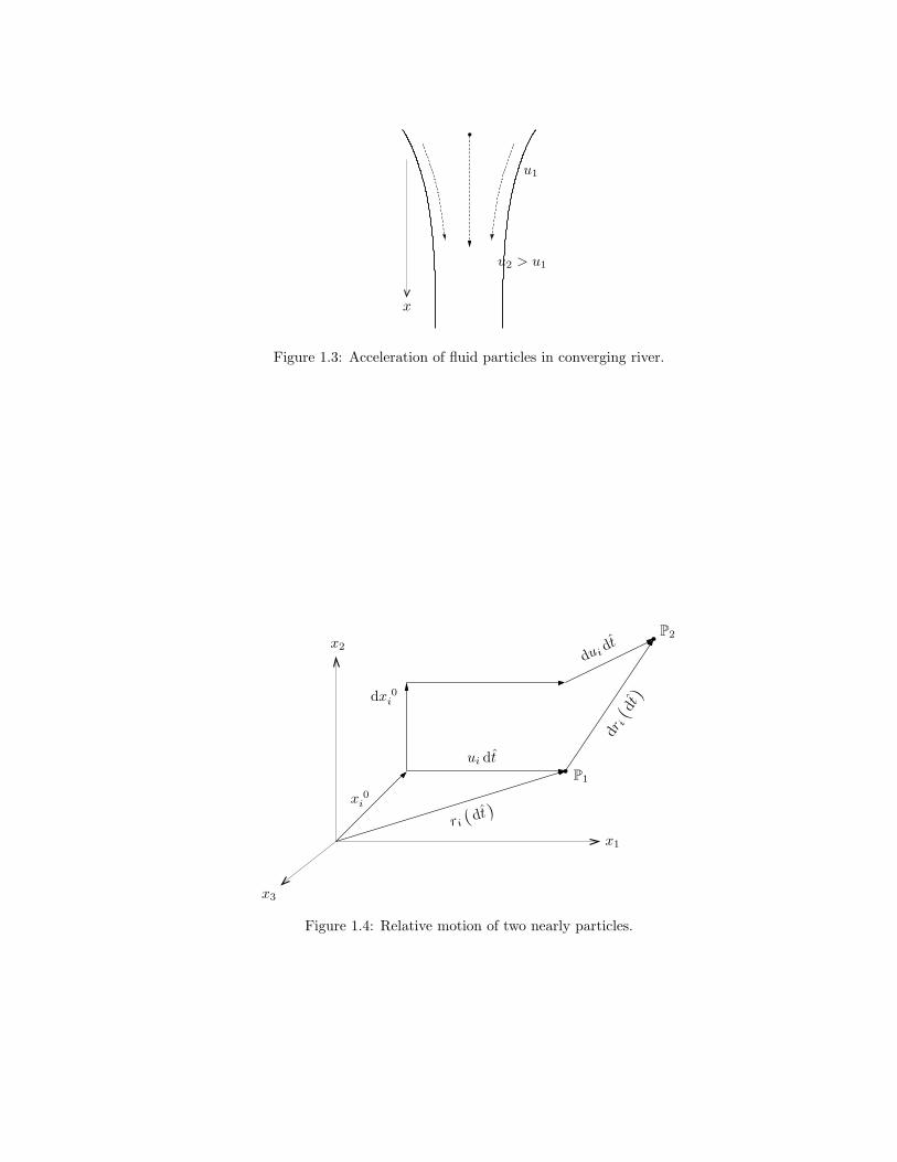
As an example we consider the acceleration of a fluid particle in a steady converging river, see figure1.3. The acceleration is defined
aj =DuiDt
=∂ui∂t
+ uj∂ui∂xj
which can be simplified in 1D for stationary case to
a =Du
Dt=∂u
∂t+ u
∂u
∂x
Note that the acceleration 6= 0 even if velocity at fixed x does not change. This has been experiencedby everyone in a raft in a converging river. The raft which is following the fluid is accelerating althoughthe flow field is steady.
Description of deformation
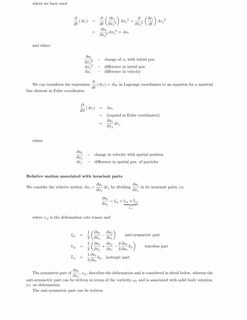
Evolution of a line element
Consider the two nearby particles in figure 1.4 during time dt. The position of P2 can by Taylor expansionbe expressed as
P2 : ri(dt)+ dri
(dt)=
= ri (0) +∂ri
∂t(0) dt+ dri (0) +
∂∂t( dri)
∣∣∣0dt
= xi0 + dxi
0 + ui (0) dt+ dui (0) dt
10 CHAPTER 1. DERIVATION OF THE NAVIER-STOKES EQUATIONS
PSfrag replacements
x, x1y, x2z, x3u, u1v, u2w, u3x1x2x 0i
ri(x 0i , t
)
ui(x 0i , t
)
P(t = 0
)
x
u1
u2 > u1
Figure 1.3: Acceleration of fluid particles in converging river.
PSfrag replacements
x, x1y, x2z, x3u, u1v, u2w, u3x1x2x 0i
ri(x 0i , t
)
ui(x 0i , t
)
P(t = 0
)
xu1
u2 > u1
x1
x2
x3
x 0i
ui dt
dx 0i
duidt
ri(dt)
dri( dt)
P1
P2
Figure 1.4: Relative motion of two nearly particles.
1.2. KINEMATICS 11
where we have used
∂
∂t( dri) =
∂
∂t
(∂ri∂xj0
)
dxj0 =
∂
∂xj0
(∂ri
∂t
)
dxj0
=∂ui∂xj0
dxj0 = dui
and where
∂ui∂xj0
− change of ui with initial pos.
dxj0 − difference in initial pos.
dui − difference in velocity
We can transform the expression∂
∂t( dri) = dui in Lagrange coordinates to an equation for a material
line element in Euler coordinates
D
Dt( dri) = dui
= expand in Euler coordinates
=∂ui∂xj
drj
where
∂ui∂xj
− change in velocity with spatial position
drj − difference in spatial pos. of particles
Relative motion associated with invariant parts
We consider the relative motion dui =∂ui∂xj
drj by dividing∂ui∂xj
in its invariant parts, i.e.
∂ui∂xj
= ξij + eij + eij︸ ︷︷ ︸
eij
where eij is the deformation rate tensor and
ξij =1
2
(∂ui∂uj
− ∂uj∂xi
)
anti-symmetric part
eij =1
2
(∂ui∂xj
+∂uj∂xi
− 23
∂ur∂ur
δij
)
traceless part
eij =1
3
∂ur∂ur
δij isotropic part
The symmetric part of∂ui∂xj
, eij , describes the deformation and is considered in detail below, whereas the
anti-symmetric part can be written in terms of the vorticity ωk and is associated with solid body rotation,i.e. no deformation.
The anti-symmetric part can be written

12 CHAPTER 1. DERIVATION OF THE NAVIER-STOKES EQUATIONS
PSfrag replacements
x, x1y, x2z, x3u, u1v, u2w, u3x1x2x 0i
ri(x 0i , t
)
ui(x 0i , t
)
P(t = 0
)
xu1
u2 > u1x1x2x3x 0i
ui dtdx 0
i
dui dtri(dt)
dri(dt)
P1
P2
x1
x2
x3
R3
R2
R1
r3
r2
r1
π2 + dϕ12
Figure 1.5: Deformation of a cube.
[ξij ] =
0 12
(∂u1∂x2
− ∂u2∂x1
)12
(∂u1∂x3
− ∂u3∂x1
)
− 12
(∂u1∂x2
− ∂u2∂x1
)
0 12
(∂u2∂x3
− ∂u3∂x2
)
− 12
(∂u1∂x3
− ∂u3∂x1
)
− 12
(∂u2∂x3
− ∂u3∂x2
)
0
= use ω = ∇× u , ωk = εkji∂
∂xjui
=
0 − 12ω3
12ω2
12ω3 0 − 1
2ω112ω2
12ω1 0
Deformation of a small cube
Consider the deformation of the small cube in figure 1.5, where we define
Rlk = Rδkl component k of side l
rlk = Rlk +∂uk∂xj
Rlj︸ ︷︷ ︸
dulk
dt relative motion of side l
= R
(
δkl +∂uk∂xl
dt
)
deformed cube
First, we consider the deformation on side 1, which can be expressed as
dR1 =∣∣∣r1∣∣∣− R =
√
r1kr1k − R
The inner product can be expanded as
r1kr1k =
[(
1 +∂u1∂x1
dt
)2
+
(∂u2∂x1
dt
)2
+
(∂u3∂x1
dt
)2]
R2
= drop quadratic terms
= R2(
1 + 2∂u1∂x1
dt
)
1.2. KINEMATICS 13
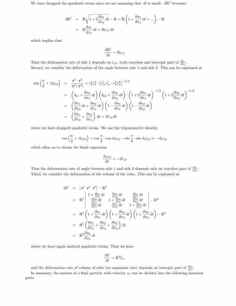
We have dropped the quadratic terms since we are assuming that dt is small. dR1 becomes
dR1 = R
√
1 + 2∂u1∂x1
dt− R = R(
1 +∂u1∂x1
dt+ ...
)
− R
= R∂u1∂x1
dt = Re11 dt
which implies that
dR1
dt= Re11
Thus the deformation rate of side 1 depends on e11, both traceless and isotropic part of∂ui
∂xj.
Second, we consider the deformation of the angle between side 1 and side 2. This can be expressed as
cos(π
2+ dφ12
)
=r1 · r2|r1| |r2| = r1kr
2k ·(r1mr
1m · r2nr2n
)−1/2
=
(
δk1 +∂uk∂x1
dt
)(
δk2 +∂uk∂x2
dt
)
·(
1 + 2∂u1∂x1
dt
)−1/2(
1 + 2∂u2∂x2
dt
)−1/2
=
(∂u1∂x2
dt+∂u2∂x1
dt
)(
1− ∂u1∂x1
dt
)(
1− ∂u2∂x2
dt
)
=
(∂u1∂x2
+∂u2∂x1
)
dt = 2e12 dt
where we have dropped quadratic terms. We use the trigonometric identity
cos(π
2+ dϕ12
)
= cosπ
2· cos dϕ12 − sin
π
2· sin dϕ12 ≈ −dϕ12
which allow us to obtain the finial expression
dϕ12dt
= −2e12
Thus the deformation rate of angle between side 1 and side 2 depends only on traceless part of ∂ui
∂xj.
Third, we consider the deformation of the volume of the cube. This can be expressed as
dV =∣∣ r1 r2 r3
∣∣− R3
= R3
∣∣∣∣∣∣∣
1 + ∂u1∂x1
dt ∂u1∂x2
dt ∂u1∂x3
dt∂u2∂x1
dt 1 + ∂u2∂x2
dt ∂u2∂x3
dt∂u3∂x1
dt ∂u3∂x2
dt 1 + ∂u3∂x3
dt
∣∣∣∣∣∣∣
− R3
= R3(
1 +∂u1∂x1
dt
)(
1 +∂u2∂x2
dt
)(
1 +∂u3∂x3
dt
)
− R3
= R3(∂u1∂x1
+∂u2∂x2
+∂u3∂x3
)
dt
= R3∂uk∂xk
dt
where we have again omitted quadratic terms. Thus we have
dV
dt= R3err
and the deformation rate of volume of cube (or expansion rate) depends on isotropic part of ∂ui
∂xj.
In summary, the motion of a fluid particle with velocity ui can be divided into the following invariantparts
14 CHAPTER 1. DERIVATION OF THE NAVIER-STOKES EQUATIONS
PSfrag replacements
x, x1y, x2z, x3u, u1v, u2w, u3x1x2x 0i
ri(x 0i , t
)
ui(x 0i , t
)
P(t = 0
)
xu1
u2 > u1x1x2x3x 0i
ui dtdx 0
i
dui dtri(dt)
dri(dt)
P1
P2
x1x2x3R3
R2
R1
r3
r2
r1π2 + dϕ12
V (t)
S(t)
V (t+∆t)− V (t)
S (t+∆t)
u
n
V (t+∆t)
Figure 1.6: Volume moving with the fluid.
i) ui solid body translation
ii) ξij =12
(∂ui∂xj
− ∂uj∂xi
)
= − 12εkijωk solid body rotation
iii) eij =12
(∂ui∂xj
+∂uj∂xi
− 23
∂ur∂ur
δij
)
volume constant deformation
iv) eij =13
∂ur∂ur
δij volume expansion rate
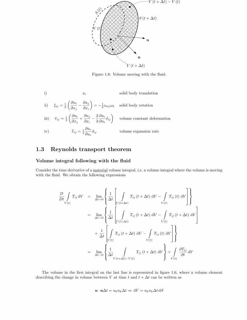
1.3 Reynolds transport theorem
Volume integral following with the fluid
Consider the time derivative of a material volume integral, i.e. a volume integral where the volume is movingwith the fluid. We obtain the following expressions
D
Dt
∫
V (t)
Tij dV = lim∆t→0
1
∆t
∫
V (t+∆t)
Tij (t+∆t) dV −∫
V (t)
Tij (t) dV
= lim∆t→0
1
∆t
∫
V (t+∆t)
Tij (t+∆t) dV −∫
V (t)
Tij (t+∆t) dV
+1
∆t
∫
V (t)
Tij (t+∆t) dV −∫
V (t)
Tij (t) dV
= lim∆t→0
1
∆t
∫
V (t+∆t)−V (t)
Tij (t+∆t) dV
+
∫
V (t)
∂Tij∂t
dV
The volume in the first integral on the last line is represented in figure 1.6, where a volume elementdescribing the change in volume between V at time t and t+∆t can be written as
u · n∆t = uknk∆t⇒ dV = uknk∆tdS
1.4. MOMENTUM EQUATION 15
This implies that the volume integral can be converted to a surface integral. This surface integral canin turn be changed back to a volume integral by the use of Gauss (or Greens) theorem. We have
D
Dt
∫
V (t)
Tij dV = lim∆t→0
[∮
S(t)
Tij (t+∆t)uknk dS
]
+
∫
V (t)
∂Tij∂t
dV
=
∮
S(t)
Tijuknk dS +
∫
V (t)
∂Tij∂t
dV = Gauss/Green’s theorem
=
∫
V (t)
[∂Tij∂t
+∂
∂xk(ukTij)
]
dV
which is the Reynolds transport theorem.
Conservation of mass
By the substitution Tij → ρ and the use of the Reynolds transport theorem above we can derive theequation for the conservation of mass. We have
D
Dt
∫
V (t)
ρdV =
∫
V (t)
[∂ρ
∂t+
∂
∂xk(ukρ)
]
= 0
Since the volume is arbitrary, the following must hold for the integrand
0 =∂ρ
∂t︸︷︷︸
©1
+∂
∂xk(ukρ)
︸ ︷︷ ︸
©2
=∂ρ
∂t+ uk
∂ρ
∂xk+ ρ
∂uk∂xk
=Dρ
Dt︸︷︷︸
©3
+ ρ∂uk∂xk︸ ︷︷ ︸
©4where we have used the definition of the material derivative in order to simplify the expression. The
terms in the expression can be given the following interpretations:
©1 : accumulation of mass in fixed element©2 : net flow rate of mass out of element©3 : rate of density change of material element©4 : volume expansion rate of material element
By considering the transport of a quantity given per unit mass, i.e. Tij = ρtij , we can simplify Reynoldstransport theorem. The integrand in the theorem can then be written
∂
∂t(ρtij) +
∂
∂xk(ukρ tij) = tij
¢¢¢
0 (cont. eq.)
∂ρ
∂t+ ρ
∂tij∂t
+ tij©©
©©©*0∂
∂xk(ukρ) + ρuk
∂tij∂xk
= ρDtijDt
which implies that Reynolds transport theorem becomes
D
Dt
∫
V (t)
ρ tij dV =
∫
V (t)
ρDtijDt
dV
where V (t) again is a material volume.
1.4 Momentum equation
Conservation of momentum
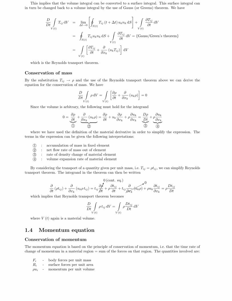
The momentum equation is based on the principle of conservation of momentum, i.e. that the time rate ofchange of momentum in a material region = sum of the forces on that region. The quantities involved are:
Fi - body forces per unit massRi - surface forces per unit areaρui - momentum per unit volume

16 CHAPTER 1. DERIVATION OF THE NAVIER-STOKES EQUATIONS
PSfrag replacements
x, x1y, x2z, x3u, u1v, u2w, u3x1x2x 0i
ri(x 0i , t
)
ui(x 0i , t
)
P(t = 0
)
xu1
u2 > u1x1x2x3x 0i
ui dtdx 0
i
dui dtri(dt)
dri(dt)
P1
P2
x1x2x3R3
R2
R1
r3
r2
r1π2 + dϕ12
V (t)S (t)
V (t+∆t)− V (t)S (t+∆t)
un
V (t+∆t)
dS
∆s(k)
︷︸︸︷
nInII
nIII(k)
R(nI)
R(nII)
dl
Figure 1.7: Momentum balance for fluid element
R
PSfrag replacements
x, x1y, x2z, x3u, u1v, u2w, u3x1x2x 0i
ri(x 0i , t
)
ui(x 0i , t
)
P(t = 0
)
xu1
u2 > u1x1x2x3x 0i
ui dtdx 0
i
dui dtri(dt)
dri(dt)
P1
P2
x1x2x3R3
R2
R1
r3
r2
r1π2 + dϕ12
V (t)S (t)
V (t+∆t)− V (t)S (t+∆t)
un
V (t+∆t)
n
R
Figure 1.8: Surface force and unit normal.
We can put the momentum conservation in integral form as follows
D
Dt
∫
V (t)
ρui dV =
∫
V (t)
ρFi dV +
∫
S(t)
Ri dS
Using Reynolds transport theorem this can be written
∫
V (t)
ρDuiDt
dV =
∫
V (t)
ρFi dV +
∫
S(t)
Ri dS
which is Newtons second law written for a volume of fluid: mass · acceleration = sum of forces. Toproceed Ri must be investigated so that the surface integral can be transformed to a volume integral. Inorder to do that we have to define the stress tensor.
The stress tensor
Remove a fluid element and replace outside fluid by surface forces as in figure 1.7. Here R(n) is the surfaceforce per unit area on surface dS with normal n, see figure 1.8. Momentum conservation for the small fluidparticle leads to
ρDuiDt
dS dl = ρFi dS dl +Ri(nIj)dS +Ri
(nIIj)dS +
∑
k
Ri(nIII(k)j
)∆s(k) dl
Letting dl→ 0 gives
0 = Ri(nIj)dS +Ri
(nIIj)dS
Now nj = nIj = −nIIj which leads to
Ri (nj) = −Ri (−nj)implying that a surface force on one side of a surface is balanced by an equal an opposite surface force
at the other side of that surface. Note that it is a general principle that the terms proportional to thevolume of a small fluid particle approaches zero faster than the terms proportional to the surface area ofthe particle. Thus the surface forces acting on a small fluid particle has to balance, irrespective of volumeforces or acceleration terms.

1.4. MOMENTUM EQUATION 17
PSfrag replacements
x, x1y, x2z, x3u, u1v, u2w, u3x1x2x 0i
ri(x 0i , t
)
ui(x 0i , t
)
P(t = 0
)
xu1
u2 > u1x1x2x3x 0i
ui dtdx 0
i
dui dtri(dt)
dri(dt)
P1
P2
x1x2x3R3
R2
R1
r3
r2
r1π2 + dϕ12
V (t)S (t)
V (t+∆t)− V (t)S (t+∆t)
un
V (t+∆t)
T11
T21
T31
x1
R(e1) = (T11, T21, T31)
Figure 1.9: Definition of surface force components on a surface with a normal in the 1-direction.
PSfrag replacements
x, x1y, x2z, x3u, u1v, u2w, u3x1x2x 0i
ri(x 0i , t
)
ui(x 0i , t
)
P(t = 0
)
xu1
u2 > u1x1x2x3x 0i
ui dtdx 0
i
dui dtri(dt)
dri(dt)
P1
P2
x1x2x3R3
R2
R1
r3
r2
r1π2 + dϕ12
V (t)S (t)
V (t+∆t)− V (t)S (t+∆t)
un
V (t+∆t)
T12
T22
T32
x2R(e2) = (T12, T22, T32)
Figure 1.10: Definition of surface force components on a surface with a normal in the 2-direction.
We now divide the surface forces into components along the coordinate directions, as in figures 1.9 and1.10, with corresponding definitions for the force components on a surface with a normal in the 3-direction.Thus, Tij is the i-component of the surface force on a surface dS with a normal in the j-direction.
Consider a fluid particle with surfaces along the coordinate directions cut by a slanted surface, as infigure 1.11. The areas of the surface elements are related by
dSj = ej · ndS = nj dS
where dS is the area of the slanted surface. Momentum balance require the surface forces to balancein the element, we have
0 = R1 dS − T11n1 dS − T12n2 dS − T13n3 dSwhich implies that the total surface force Ri can be written in terms of the components of the stress
tensor Tij as
Ri = Ti1n1 + Ti2n2 + Ti3n3 = Tijnj
PSfrag replacements
x, x1y, x2z, x3u, u1v, u2w, u3x1x2x 0i
ri(x 0i , t
)
ui(x 0i , t
)
P(t = 0
)
xu1
u2 > u1x1x2x3x 0i
ui dtdx 0
i
dui dtri(dt)
dri(dt)
P1
P2
x1x2x3R3
R2
R1
r3
r2
r1π2 + dϕ12
V (t)S (t)
V (t+∆t)− V (t)S (t+∆t)
un
V (t+∆t)
e1
e2
e3
R
R1
n
dS1dS2
dS3
Figure 1.11: Surface force balance on a fluid particle with a slanted surface.

18 CHAPTER 1. DERIVATION OF THE NAVIER-STOKES EQUATIONS
Here the diagonal components are normal stresses off-diagonal components are shear stresses.Further consideration of the moment balance around a fluid particle show that Tij is a symmetric tensor,
i.e.
Tij = Tji
Momentum equation
Using the definition of the surface force in terms of the stress tensor, the momentum equation can now bewritten
∫
V (t)
ρDuiDt
dV =
∫
V (t)
ρFi dV +
∫
S(t)
Tijnj dS =
∫
V (t)
[
ρFi +∂Tij∂xj
]
dV
The volume is again arbitrary implying that the integrand must itself equal zero. We have
ρDuiDt
= ρFi +∂Tij∂xj
Pressure and viscous stress tensor
For fluid at rest only normal stresses present otherwise fluid element would deform. We thus divide thestress tensor into an isotropic part, the hydrodynamic pressure p, and a part depending on the motion ofthe fluid. We have
PSfrag replacements
x, x1y, x2z, x3u, u1v, u2w, u3x1x2x 0i
ri(x 0i , t
)
ui(x 0i , t
)
P(t = 0
)
xu1
u2 > u1x1x2x3x 0i
ui dtdx 0
i
dui dtri(dt)
dri(dt)
P1
P2
x1x2x3R3
R2
R1
r3
r2
r1π2 + dϕ12
V (t)S (t)
V (t+∆t)− V (t)S (t+∆t)
un
V (t+∆t)p
p
p
Tij = −pδij + τijp - hydrodynamic pressure, directed inwardτij - viscous stress tensor, depends on fluid motion
Newtonian fluid
It is natural to assume that the viscous stresses are functions of deformation rate eij or strain. Recall thatthe invariant symmetric parts are
eij =1
2
(∂ui∂xj
+∂uj∂xi
− 23
∂ur∂xr
δij
)
︸ ︷︷ ︸
eij
+1
3
∂ur∂xr
δij︸ ︷︷ ︸
eij
where eij is the volume constant deformation rate and eij is the uniform rate of expansion. For anisotropic fluid, the viscous stress tensor is a linear function of the invariant parts of eij , i.e.
τij = λeij + 2µeij
where we have defined the two viscosities as
µ (T ): dynamic viscosity (here T is the temperature)λ (T ): second viscosity, often=0
For a Newtonian fluid, we thus have the following relationship between the viscous stress and the strain(deformation rate)
τij = 2µeij = µ
(∂ui∂xj
+∂uj∂xi
− 23
∂ur∂xr
δij
)
which leads to the momentum equation
ρDuiDt
= − ∂p
∂xi+
∂
∂xj
[
µ
(∂ui∂xj
+∂uj∂xi
− 23
∂ur∂xr
δij
)]
+ ρFi

1.5. ENERGY EQUATION 19
1.5 Energy equation
The energy equation is a mathematical statement which is based on the physical law that the rate of changeof energy in material particle = rate that energy is received by heat and work transfers by that particle.We have the following definitions
ρ[e+ 1
2uiui]dV energy of particle, with e the internal energy
ρuiFi dV work rate︸ ︷︷ ︸
force · velocity
of Fi on particle
ujRj dS work rate of Rj on particle
niqi dS heat loss from surface, with qi the heat flux vector, directed outward
Using Reynolds transport theorem we can put the energy conservation in integral form as
D
Dt
∫
V (t)
ρ
[
e+1
2uiui
]
dV =
∫
V (t)
ρFiui dV +
∫
S(t)
[niTijuj − niqi] dS =∫
V (t)
[
ρFiui +∂
∂xi(Tijuj − qi)
]
dV
Compare the expression in classical mechanics, where the momentum equation is mu = F and theassociated kinetic energy equation is
m2
ddt (u · u) = F · u
work rate = force · velocity( work = force · dist. )
From the integral energy equation we obtain the total energy equation by the observation that thevolume is arbitrary and thus that the integrand itself has to be zero. We have
ρD
Dt
(
e+1
2uiui
)
= ρFiui −∂
∂xi(pui) +
∂
∂xi(τijuj)−
∂qi∂xi
The mechanical energy equation is found by taking the dot product between the momentum equationand u. We obtain
ρD
Dt
(1
2uiui
)
= ρFiui − ui∂p
∂xi+ ui
∂τij∂xj
Thermal energy equation is then found by subtracting the mechanical energy equation from the totalenergy equation, i.e.
ρDe
Dt= −p∂ui
∂xi+ τij
∂ui∂xj
− ∂qi∂xi
The work of the surface forces divides into viscous and pressure work as follows
− ∂
∂xi(pui) = −p∂ui
∂xi− ui
∂p
∂xi
©1 ©2
∂
∂xi(τijuj) = τij
∂ui∂xj
+ uj∂τij∂xi
where following interpretations can be given to the thermal and the mechanical terms
©1 : thermal terms( force · deformation ): heat generated by compression and viscous dissipation
©2 : mechanical terms( velocity · force gradients ): gradients accelerate fluid and increase kinetic energy

20 CHAPTER 1. DERIVATION OF THE NAVIER-STOKES EQUATIONS
The heat flux need to be related to the temperature gradients with Fouriers law
qi = −κ∂T
∂xi
where κ = κ (T ) is the thermal conductivity. This allows us to write the thermal energy equation as
ρDe
Dt= −p∂ui
∂xi+Φ+
∂
∂xi
(
κ∂T
∂xi
)
where the positive definite dissipation function Φ is defined as
Φ = τij∂ui∂xj
= 2µ
[
eijeij −1
3
(∂uk∂xk
)2]
= 2µ
(
eij −1
3
∂uk∂xk
δij
)2
> 0
Alternative form of the thermal energy equation can be derived using the definition of the enthalpy
h = e+p
ρ
We have
Dh
Dt=De
Dt+1
ρ
Dp
Dt− p
ρ2Dρ
Dt︸︷︷︸
−(
ρ∂ui∂xi
)
which gives the final result
ρDh
Dt=Dp
Dt+Φ+
∂
∂xi
(
κ∂T
∂xi
)
To close the system of equations we need a
i) thermodynamic equation e = e (T, p) simplest case: e = cvT or h = cpT
ii) equation of state p = ρRT
where cv and cp are the specific heats at constant volume and temperature, respectively. At this timewe also define the ratio of the specific heats as
γ =cpcv
1.6 Navier-Stokes equations
The derivation is now completed and we are left with the Navier-Stokes equations. They are the equationdescribing the conservation of mass, the equation describing the conservation of momentum and the equationdescribing the conservation of energy. We have
Dρ
Dt+ ρ
∂uk∂xk
= 0
ρDuiDt
= − ∂p
∂xi+∂τij∂xj
+ ρFi
ρDe
Dt= −p∂ui
∂xi+Φ+
∂
∂xi
(
κ∂T
∂xi
)
where

1.6. NAVIER-STOKES EQUATIONS 21
Φ = τij∂ui∂xj
τij = µ
(∂ui∂xj
+∂uj∂xi
− 23
∂ur∂xr
δij
)
and the thermodynamic relation and the equation of state for a gas
e = e (T, p)
p = ρRT
We have 7 equations and 7 unknowns and therefore the necessary requirements to obtain a solution ofthe system of equations.
unknown equationsρ 1 continuity 1ui 3 momentum 3p 1 energy 1e 1 thermodyn. 1T 1 gas law 1
∑7
∑7
Equations in conservative form
A slightly different version of the equations can be found by using the identity
ρDtijDt
=∂
∂t(ρtij) +
∂
∂xk(ukρtij)
to obtain the system
∂ρ
∂t+
∂
∂xk(ukρ) = 0
∂
∂t(ρui) +
∂
∂xk(ρukui) = −
∂p
∂xi+∂τij∂xj
+ ρFi
∂
∂t
(
e+1
2uiui
)
+∂
∂xk
[
ρuk
(
e+1
2uiui
)]
= ρFiui −∂
∂xi(pui) +
∂
∂xi(τijuj) +
∂
∂xi
(
κ∂T
∂xi
)
These are all of the form
∂U
∂t+∂G(i)
∂xi= J or
∂U
∂t+∂G
∂x+∂G
∂y+∂G
∂z= J
where
U = (ρ, ρu1, ρu2, ρu3, ρ (e+ uiui/2))T
is the vector of unknowns,
J = (0, ρF1, ρF2, ρF3, ρuiFi)T
is the vector of the right hand sides and
G(i) =
ρuiρu1ui + pδ1i − τ1iρu2ui + pδ2i − τ2iρu3ui + pδ3i − τ3iρ (e+ uiui/2)ui + pui + κ
∂T∂xi
− ujτij
is the flux of mass, momentum and energy, respectively. This form of the equation is usually termedthe conservative form of the Navier-Stokes equations.

22 CHAPTER 1. DERIVATION OF THE NAVIER-STOKES EQUATIONS
1.7 Incompressible Navier-Stokes equations
The conservation of mass and momentum can be written
Dρ
Dt+ ρ
∂ui∂xi
= 0
ρDuiDt
= − ∂p
∂xi+∂τij∂xj
+ ρFi
τij = µ
(∂ui∂xj
+∂uj∂xi
− 23
∂uk∂uk
δij
)
for incompressible flow ρ = constant, which from the conservation of mass equation implies
∂ui∂xi
= 0
implying that a fluid particle experiences no change in volume. Thus the conservation of mass andmomentum reduce to
∂ui∂t
+ uj∂ui∂xj
= −1ρ
∂p
∂xi+ ν∇2ui + Fi
∂ui∂xi
= 0
since the components of the viscous stress tensor can now be written
∂
∂xj
(∂ui∂xj
+∂uj∂xi
− 23
∂uk∂xk
δij
)
=∂2ui∂xj∂xj
= ∇2ui
We have also introduced the kinematic viscosity, ν, above, defined as
ν = µ/ρ
The incompressible version of the conservation of mass and momentum equations are usually referredto as the incompressible Navier-Stokes equations, or just the Navier-Stokes equations in case it is evidentthat the incompressible limit is assumed. The reason that the energy equation is not included in theincompressible Navier-Stokes equations is that it decouples from the momentum and conservation of massequations, as we will see below. In addition it can be worth noting that the conservation of mass equationis sometimes referred to as the continuity equation.
The incompressible Navier-Stokes equations need boundary and initial conditions in order for a solutionto be possible. Boundary conditions (BC) on solid surfaces are ui = 0. They are for obvious reasons usuallyreferred to as the no slip conditions. As initial condition (IC) one needs to specify the velocity field at theinitial time ui (t = 0) = u0i . The pressure field does not need to be specified as it can be obtained once thevelocity field is specified, as will be discussed below.
Integral form of the Navier-Stokes eq.
We have derived the differential form of the Navier-Stokes equations. Sometimes, for example when afinite-volume discretization is derived, it is convenient to use an integral form of the equations.
An integral from of the continuity equation is found by integrating the divergence constraint over afixed volume VF and using the Gauss theorem. We have
∫
V
∂
∂xi(ui) dVF =
∫
S
uini dSF = 0
An integral form of the momentum equation is found by taking the time derivative of a fixed volumeintegral of the velocity, substituting the differential form of the Navier-Stokes equation, using the continuityequation and Gauss theorem. We have
∂
∂t
∫
VF
ui dV =
∫
VF
∂ui∂t
dV = −∫
VF
[∂
∂xj(ujui) +
1
ρ
∂p
∂xi− ν ∂2ui
∂xj∂xj
]
dV =
−∫
VF
∂
∂xj
[
ujui +1
ρpδij − ν
∂ui∂xj
]
dV = −∫
SF
[
uiujnj +p
ρni − ν
∂ui∂xj
nj
]
dS

1.7. INCOMPRESSIBLE NAVIER-STOKES EQUATIONS 23
PSfrag replacements
x, x1y, x2z, x3u, u1v, u2w, u3x1x2x 0i
ri(x 0i , t
)
ui(x 0i , t
)
P(t = 0
)
xu1
u2 > u1x1x2x3x 0i
ui dtdx 0
i
dui dtri(dt)
dri(dt)
P1
P2
x1x2x3R3
R2
R1
r3
r2
r1π2 + dϕ12
V (t)S (t)
V (t+∆t)− V (t)S (t+∆t)
un
V (t+∆t)
p
T0, U0
Tw
Tw
L
L
T0 U0
Figure 1.12: Examples of length, velocity and temperature scales.
Note that the integral from of the continuity equation is a compatibility condition for BC in incom-pressible flow.
Dimensionless form
It is often convenient to work with a non-dimensional form of the Navier-Stokes equations. We use thefollowing scales and non-dimensional variables
x∗i =xiL
t∗ =tU0L
u∗i =uiU0
p∗ =p
p0
∂
∂xi=1
L
∂
∂x∗i
∂
∂t=U0L
∂
∂t∗⇒
where ∗ signifies a non-dimensional variable. The length and velocity scales have to be chosen appropri-ately from the problem under investigation, so that they represent typical lengths and velocities present.See figure 1.12 for examples.
If we introduce the non-dimensional variables in the Navier-Stokes equations we find
U20
L· ∂u
∗i
∂t∗+U20
Lu∗j∂u∗i∂x∗j
= − p0ρL
∂p∗
∂x∗i+νU0L2
∂2u∗i∂x∗j∂x
∗j
U0L· ∂u
∗i
∂x∗i= 0
Now drop * as a sign of non-dimensional variables and divide through with U 20 /L, we find
∂ui∂t
+ uj∂ui∂xj
= − p0ρU2
0
∂p
∂xi+
ν
U0L∇2ui
∂ui∂xi
= 0
We have defined the Reynolds number Re as
Re =U0L
ν=
U20 /L
νU0/L2“inertial forces”
“viscous forces”
which can be interpreted as a measure of the inertial forces divided by the viscous forces. The Reynoldsnumber is by far the single most important non-dimensional number in fluid mechanics. We also define thepressure scale as
p0 = ρU20
which leaves us with the final form of the non-dimensional incompressible Navier-Stokes equations as
∂ui∂t
+ uj∂ui∂xj
= − ∂p
∂xi+1
Re∇2ui
∂ui∂xi
= 0
24 CHAPTER 1. DERIVATION OF THE NAVIER-STOKES EQUATIONS
Non-dimensional energy equation
We stated above that the energy equation decouple from the rest of the Navier-Stokes equations for in-compressible flow. This can be seen from a non-dimensionalization of the energy equation. We use thedefinition of the enthalpy (h = cpT ) to write the thermal energy equation as
ρcpDT
Dt=Dp
Dt+Φ+ κ∇2T
and use the following non-dimensional forms of the temperature and dissipation function
T ∗ =T − T0Tw − T0
Φ∗ =L2
U20µΦ
This leads to
DT ∗
Dt∗=
µ
ρU0L· κ
µcp· ∇∗2T ∗ +
U20
cp (Tw − T0)
[Dp∗
Dt∗+
µ
ρU0Lφ∗]
=1
Re· 1Pr
· ∇∗2T ∗ +U20
cp (Tw − T0)︸ ︷︷ ︸
Ma2a20
cp(Tw−T0)
(Dp∗
Dt∗+1
RΦ∗)
where a0 speed of sound in free-stream andMa =U0a0is Mach number. We now drop ∗ and letMa→ 0
to obtain
DT
Dt=
1
Re· 1Pr
· ∇2T
where the Prandtl number Pr =µcp
κ , which takes on a value of ≈ 0.7 for air.As the Mach number approaches zero, the fluid behaves as an incompressible medium, which can be
seen from the definition of the speed of sound. We have
a0 =γ
ρα, α =
1
ρ
∂ρ
∂p
∣∣∣∣T
where α is the isothermal compressibility coefficient. If the density is constant, not depending on p, wehave that α→ 0 and a0 →∞, which implies that Ma→ 0.
1.8 Role of the pressure in incompressible flow
The role of the pressure in incompressible flow is special due to the absence of a time derivative in thecontinuity equation. We will illustrate this in two different ways.
Artificial compressibility
First we discuss the artificial compressibility version of the equations, used sometimes for solution of thesteady equations. We define a simplified continuity equation and equation of state as
∂ρ
∂t+∂ui∂xi
= 0 and p = βρ
This allows us to write the Navier-Stokes equations as
∂ui∂t
+∂
∂xj(ujui) = − ∂p
∂xi+1
Re∇2ui
∂p
∂t+ β
∂ui∂xi
= 0
Let
u =
puvw
e =
βup+ u2
uvuw
f =
βvuv
p+ v2
vw
g =
βwuwvw
p+ β2

1.8. ROLE OF THE PRESSURE IN INCOMPRESSIBLE FLOW 25
be the vector of unknowns and their fluxes. The Navier-Stokes equations can then be written
∂u
∂t+∂e
∂x+∂f
∂y+∂g
∂z=
1
Re∇2Du
or∂u
∂t+A
∂u
∂x+B
∂u
∂y+C
∂u
∂z=
1
R∇2Du
where the matrices above are defined
A =∂e
∂u=
0 β 0 01 2u 0 00 v u 00 w 0 u
, B =
∂f
∂u=
0 0 β 00 v u 01 0 2v 00 0 w v
C =∂g
∂u=
0 0 0 β0 v u 01 0 2v 00 0 w v
, D =
0 0 0 00 1 0 00 0 1 00 0 0 1
the eigenvalues of A,B,C are the wave speeds of plane waves in the respective coordinate directions,they are
(
u, u, u±√
u2 + β)
,(
v, v, v ±√
v2 + β)
and(
w,w,w ±√
w2 + β)
Note that the effective acoustic or pressure wave speed ∼ √β →∞ for incompressible flow.
Projection on a divergence free space
Second we discuss the projection of the velocity field on a divergence free space. We begin by the followingtheorem.
Theorem 1. Any wi in Ω can uniquely be decomposed into
wi = ui +∂p
∂xi
where∂ui∂xi
= 0, ui · ni = 0 on ∂Ω.
i.e. into a function ui that is divergence free and parallel to the boundary and the gradient of a function,here called p.
Proof. We start by showing that ui and∂p
∂xiis orthogonal in the L2 inner product.
(
ui,∂p
∂xi
)
=
∫
Ω
ui∂p
∂xidV =
∫
Ω
∂
∂xi(uip) dV =
∮
∂Ω
puini dS = 0
The uniqueness of the decomposition can be seen by assuming that we have two different decompositionsand showing that they have to be equivalent. Let
wi = u(1)i +
∂p(1)
∂xi= u
(2)i +
∂p(2)
∂xi
The inner product between
u(1)i − u(2)i +
∂
∂xi
(
p(1) − p(2))
and u(1)i − u(2)i
gives
0 =
∫
Ω
[(
u(1)i − u(2)i
)2
+(
u(1)i − u(2)i
) ∂
∂xi
(
p(1) − p(2))]
dV =
∫
Ω
(
u(1)i − u(2)i
)2
dV
Thus we haveu(1)i = u
(2)i , p(1) = p(2) + C

26 CHAPTER 1. DERIVATION OF THE NAVIER-STOKES EQUATIONS
PSfrag replacements
x, x1y, x2z, x3u, u1v, u2w, u3x1x2x 0i
ri(x 0i , t
)
ui(x 0i , t
)
P(t = 0
)
xu1
u2 > u1x1x2x3x 0i
ui dtdx 0
i
dui dtri(dt)
dri(dt)
P1
P2
x1x2x3R3
R2
R1
r3
r2
r1π2 + dϕ12
V (t)S (t)
V (t+∆t)− V (t)S (t+∆t)
un
V (t+∆t)
pT0, U0
TwLT0U0
Gradient fields
wi∂p∂xi
ui
Divergence free vectorfields // to boundary
Figure 1.13: Projection of a function on a divergence free space.
We can find an equation for a p with above properties by noting that
∇2p =∂wi∂xi
in Ω with∂p
∂n= wini on ∂Ω
has a unique solution. Now, if
ui = wi −∂p
∂xi⇒
we have
0 =∂ui∂xi
=∂wi∂xi
− ∂2p
∂xi∂xi; and 0 = uini = wini −
∂p
∂n
To sum up, to project wi on divergence free space let wi = ui +∂p
∂xi
1) solve for p :∂wi∂xi
= ∇2p,∂p
∂n= 0
2) let ui = wi −∂p
∂xi
This is schematically shown in figure 1.13. Note also that (wi − ui)⊥ui.
Apply to Navier-Stokes equations
Let P be orthogonal projector which maps wi on divergence free part ui, i.e. Pwi = ui. We then have thefollowing relations
wi = Pwi +∂p
∂xi
Pui = ui, P∂p
∂xi= 0
Applying the orthogonal projector to the Navier-Stokes equations, we have
P
(∂ui∂t
+∂p
∂xi
)
= P
(
−uj∂ui∂xj
+1
Re∇2ui
)
Now, ui is divergence free and parallel to boundary, thus

1.8. ROLE OF THE PRESSURE IN INCOMPRESSIBLE FLOW 27
P∂ui∂t
=∂ui∂t
However,
P∇2ui 6= ∇2ui
since ∇2ui need not be parallel to the boundary. Thus we find an evolution equation without thepressure, we have
∂ui∂t
= P
−uj
∂ui∂xj
+1
Re∇2ui
︸ ︷︷ ︸
wi
The pressure term in the Naiver-Stokes equations ensures that the right hand side wi is divergence free.We can find a Poisson equation for the pressure by taking the divergence of wi, according to the resultabove. We find
∇2p =∂
∂xi
−uj
∂ui∂xj
+1
Re∇2ui
︸ ︷︷ ︸
wi
= −∂uj
∂xi
∂ui∂xj
thus the pressure satisfies elliptic Poisson equation, which links the velocity field in the whole domaininstantaneously. This can be interpreted such that the information in incompressible flow spreads infinitelyfast, i.e. we have an infinite wave speed for pressure waves, something seen in the analysis of the artificialcompressibility equations.
Evolution equation for the divergence
It is common in several numerical solution algorithms for the Naiver-Stokes equations to discard the diver-gence constraint and instead use the pressure Poisson equation derived above as the second equation in theincompressible Naiver-Stokes equations. If this is done we may encounter solutions that are not divergencefree.
Consider the equation for the evolution of the divergence, found by taking the divergence of the mo-mentum equations and substituting the Laplacian of the pressure with the right hand side of the Poissonequation. We have
∂
∂t
(∂ui∂xi
)
=1
Re∇2
(∂ui∂xi
)
Thus the divergence is not automatically zero, but satisfies a heat equation. For the stationary case thesolution obeys the maximum principle. This states that the maximum of a harmonic function, a functionsatisfying the Laplace equation, has its maximum on the boundary. Thus, the divergence is zero inside thedomain, if and only if it is zero everywhere on the boundary.
Since it is the pressure term in the Navier-Stokes equations ensures that the velocity is divergence free,this has implications for the boundary conditions for the pressure Poisson equation. A priori we have nonespecified, but they have to be chosen such that the divergence of the velocity field is zero on the boundary.This may be a difficult constraint to satisfy in a numerical solution algorithm.

28 CHAPTER 1. DERIVATION OF THE NAVIER-STOKES EQUATIONS

Chapter 2
Flow physics
2.1 Exact solutions
Plane Pouseuille flow - exact solution for channel flow
The flow inside the two-dimensional channel, see figure 2.1, is driven by a pressure difference p0−p1 betweenthe inlet and the outlet of the channel. We will assume two-dimensional, steady flow, i.e.
∂
∂t= 0, u3 = 0
and that the flow is fully developed, meaning that effects of inlet conditions have disappeared. We have
u1 = u1 (x2) , u2 = u2 (x2)
The boundary conditions are u1 = u2 = 0 at x2 = ±h. The continuity equation reads
¶¶¶70
∂u1∂x1
+∂u2∂x2
+¶¶¶70
∂u3∂x3
= 0
where the first and the last term disappears due to the assumption of two-dimensional flow and thatthe flow is fully developed. This implies that u2 = C = 0, where the constant is seem to be zero from theboundary conditions.
The steady momentum equations read
ρu1∂u1∂x1
+ ρu2∂u1∂x2
= − ∂p
∂x1+ µ∇2u1
ρu1∂u2∂x1
+ ρu2∂u2∂x2
= − ∂p
∂x2+ µ∇2u2 − ρg
which, by applying the assumptions above, reduce to
PSfrag replacements
x, x1y, x2z, x3u, u1v, u2w, u3x1x2x 0i
ri(x 0i , t
)
ui(x 0i , t
)
P(t = 0
)
xu1
u2 > u1x1x2x3x 0i
ui dtdx 0
i
dui dtri(dt)
dri(dt)
P1
P2
x1x2x3R3
R2
R1
r3
r2
r1π2 + dϕ12
V (t)S (t)
V (t+∆t)− V (t)S (t+∆t)
un
V (t+∆t)
pT0, U0
TwLT0U0
Gradient fieldswi∂p∂xi
uiDivergence free vectorfields // to boundary
L
h
x1
x2
p0 > p1 p1
Figure 2.1: Plane channel geometry.
29

30 CHAPTER 2. FLOW PHYSICS
PSfrag replacements
x, x1y, x2z, x3u, u1v, u2w, u3x1x2x 0i
ri(x 0i , t
)
ui(x 0i , t
)
P(t = 0
)
xu1
u2 > u1x1x2x3x 0i
ui dtdx 0
i
dui dtri(dt)
dri(dt)
P1
P2
x1x2x3R3
R2
R1
r3
r2
r1π2 + dϕ12
V (t)S (t)
V (t+∆t)− V (t)S (t+∆t)
un
V (t+∆t)
pT0, U0
TwLT0U0
Gradient fieldswi∂p∂xi
uiDivergence free vectorfields // to boundary
Lhx1x2
p0 > p1p1
u
n
dS
u · n∆tFigure 2.2: Volume of fluid flowing through surface dS in time ∆t
0 = − ∂p
∂x1+ µ
d2u1dx22
0 = − ∂p
∂x2− ρg
The momentum equation in the x2-direction (or normal direction) implies
p = −ρgx2 + P (x1) ⇒ ∂p
∂x1=dP
dx1
showing that the pressure gradient in the x1-direction (or streamwise direction) is only a function ofx1. The momentum equation in the streamwise direction implies
0 = − dP
dx1+ µ
d2u1dx22
Since P (x1) and u1 (x2) we have
d2u1dx22
=1
µ
dP
dx1= const. (independent of x1, x2)
We can integrate u1 in the normal direction to obtain
u1 =1
2µ
dP
dx1x22 + C1x2 + C2
The constants can be evaluated from the boundary conditions u1 (±h) = 0, giving the parabolic velocityprofile
u1 =h2
2µ· dPdx1
[
1−(x2h
)2]
Evaluating the maximum velocity at the center of the channel we have
umax = −h2
2µ· dPdx1
> 0
if flow is in the positive x1-direction. The velocity becomes
u1umax
= 1−(x2h
)2
Flow rate
From figure 2.2 we can evaluate the flow rate as dQ = u · ndS. Integrating over the channel we find
Q =
∫
S
uini dS = channel =∫ h
−hu1 dx2 = −
2h3
3µ· dPdx1
=4
3humax

2.1. EXACT SOLUTIONS 31
PSfrag replacements
x, x1y, x2z, x3u, u1v, u2w, u3x1x2x 0i
ri(x 0i , t
)
ui(x 0i , t
)
P(t = 0
)
xu1
u2 > u1x1x2x3x 0i
ui dtdx 0
i
dui dtri(dt)
dri(dt)
P1
P2
x1x2x3R3
R2
R1
r3
r2
r1π2 + dϕ12
V (t)S (t)
V (t+∆t)− V (t)S (t+∆t)
un
V (t+∆t)
pT0, U0
TwLT0U0
Gradient fieldswi∂p∂xi
uiDivergence free vectorfields // to boundary
Lhx1x2
p0 > p1p1undS
u · n∆t
x
y
u0
p0
Figure 2.3: Stokes instantaneously plate.
Wall shear stress
The wall shear stress can be evaluated from the velocity gradient at the wall. We have
τ12 = τ21 = µdu1dx2
= −2µ · umax · x2h2
implying that
τwall = τ∣∣x2=−h =
2µumaxh
Vorticity
The vorticity is zero in the streamwise and normal directions, i.e. ω1 = ω2 = 0 and has the followingexpression in the x3-direction (or spanwise direction)
ω3 =∂u2∂x1
− ∂u1∂x2
= − du1dx2
=2umax · x2
h2
Stokes 1:st problem: instantaneously started plate
Consider the instantaneously starting plate of infinite horizontal extent shown in figure 2.3. This is a timedependent problem where plate velocity is set to u = u0 at time t = 0. We assume that the velocity can bewritten u = u(y, t) which using continuity and the boundary conditions imply that normal velocity v = 0.The momentum equations reduce to
∂u
∂t= −1
ρ
∂p
∂x+ ν
∂2u
∂y2
0 = −1ρ
∂p
∂y− g
The normal momentum equation implies that p = −ρgy + p0, where p0 is the atmospheric pressure atthe plate surface. This gives us the following diffusion equation, initial and boundary conditions for u
∂u
∂t= ν
∂2u
∂y2
u(y, 0) = 0 0 ≤ y ≤ ∞u(0, t) = u0 t > 0
u(∞, t) = 0 t > 0
We look for a similarity solution, i.e. we introduce a new dependent variable which is a combination ofy and t such that the partial differential equation reduces to an ordinary differential equation. Let

32 CHAPTER 2. FLOW PHYSICS
f(η) =u
u0η = C · y · tb
where C and b are constants to be chosen appropriately. We transform the time and space derivativesaccording to
∂
∂t=
∂η
∂t
d
dη= Cbytb−1
d
dη
∂
∂y=
∂η
∂y
d
dη= Ctb
d
dη
∂2
∂y2= C2t2b
d2
dη2
If we substitute this into the equation for u and use the definition of η, we find an equation for f
bt−1ηdf
dη= νC2t2b
d2f
dη2
where no explicit dependence on y and t can remain if a similarity solution is to exist. Thus, thecoefficient of the two η-dependent terms have to be proportional to each other, we have
bt−1 = κνC2t2b
where κ is a proportionality constant. The exponents of these expressions, as well as the coefficients infront of the t-terms have to be equal. This gives
b = −12
C =1√−2κν
We choose κ = −2 and obtain the following
f ′′ + 2ηf ′ = 0 η =y
2√νt
where ′ = ddη . The boundary and initial conditions also have to be compatible with the similarity
assumption. We have
u(y, 0)
u0= f(∞) = 0 u(0, t)
u0= f(0) = 1
u(∞, t)u0
= f(∞) = 0
This equation can be integrated twice to obtain
f = C1
∫ η
0
eξ2
dξ + C2
Using the boundary conditions and the definition of the error-function, we have
f = 1− 2√π
∫ η
0
eξ2
dξ = 1− erf(η)
This solution is shown in figure 2.4, both as a function of the similarity variable η and the unscalednormal coordinate y. Note that the time dependent solution is diffusing upward.
From the velocity we can calculate the spanwise vorticity as a function of the similarity variable η andthe unscaled normal coordinate y. Here the maximum of the vorticity is also changing in time, from theinfinite value at t = 0 it is diffusing outward in time.
ω3 = ωz =∂v
∂x− ∂u
∂y=
u0√πνt
e−η2
The vorticity is shown in figure 2.5, both as a function of the similarity variable η and the unscalednormal coordinate y. Note again that the time dependent solution is diffusing upward.
2.2 Vorticity and streamfunction
Vorticity is an important concept in fluid dynamics. It is related to the average angular momentum of afluid particle and the swirl present in the flow. However, a flow with circular streamlines may have zerovorticity and a flow with straight streamlines may have a non-zero vorticity.

2.2. VORTICITY AND STREAMFUNCTION 33
0 0.1 0.2 0.3 0.4 0.5 0.6 0.7 0.8 0.9 10
0.2
0.4
0.6
0.8
1
1.2
1.4
1.6
1.8
2
PSfrag replacements
x, x1y, x2z, x3u, u1v, u2w, u3x1x2x 0i
ri(x 0i , t
)
ui(x 0i , t
)
P(t = 0
)
xu1
u2 > u1x1x2x3x 0i
ui dtdx 0
i
dui dtri(dt)
dri(dt)
P1
P2
x1x2x3R3
R2
R1
r3
r2
r1π2 + dϕ12
V (t)S (t)
V (t+∆t)− V (t)S (t+∆t)
un
V (t+∆t)
pT0, U0
TwLT0U0
Gradient fieldswi∂p∂xi
uiDivergence free vectorfields // to boundary
Lhx1x2
p0 > p1p1undS
u · n∆txyu0p0
η = y√4νt
uu0
y = η√4νt
t0 0.1 0.2 0.3 0.4 0.5 0.6 0.7 0.8 0.9 1
0
1
2
3
4
5
6
7
8
PSfrag replacements
x, x1y, x2z, x3u, u1v, u2w, u3x1x2x 0i
ri(x 0i , t
)
ui(x 0i , t
)
P(t = 0
)
xu1
u2 > u1x1x2x3x 0i
ui dtdx 0
i
dui dtri(dt)
dri(dt)
P1
P2
x1x2x3R3
R2
R1
r3
r2
r1π2 + dϕ12
V (t)S (t)
V (t+∆t)− V (t)S (t+∆t)
un
V (t+∆t)
pT0, U0
TwLT0U0
Gradient fieldswi∂p∂xi
uiDivergence free vectorfields // to boundary
Lhx1x2
p0 > p1p1undS
u · n∆txyu0p0
η = y√4νt
uu0
y = η√4νt t
Figure 2.4: Velocity above the instantaneously started plate. a) U as a function of the similarity variableη. b) U(y, t) for various times.
0 0.1 0.2 0.3 0.4 0.5 0.6 0.7 0.8 0.9 10
0.2
0.4
0.6
0.8
1
1.2
1.4
1.6
1.8
2
PSfrag replacements
x, x1y, x2z, x3u, u1v, u2w, u3x1x2x 0i
ri(x 0i , t
)
ui(x 0i , t
)
P(t = 0
)
xu1
u2 > u1x1x2x3x 0i
ui dtdx 0
i
dui dtri(dt)
dri(dt)
P1
P2
x1x2x3R3
R2
R1
r3
r2
r1π2 + dϕ12
V (t)S (t)
V (t+∆t)− V (t)S (t+∆t)
un
V (t+∆t)
pT0, U0
TwLT0U0
Gradient fieldswi∂p∂xi
uiDivergence free vectorfields // to boundary
Lhx1x2
p0 > p1p1undS
u · n∆txyu0p0
η = y√4νtuu0
y = η√4νt
tη
y
ωz =ω(η)·u0√
πνt
t
ωz
√πνt
u0= ω(η)
0 0.1 0.2 0.3 0.4 0.5 0.6 0.7 0.8 0.9 10
1
2
3
4
5
6
7
8
PSfrag replacements
x, x1y, x2z, x3u, u1v, u2w, u3x1x2x 0i
ri(x 0i , t
)
ui(x 0i , t
)
P(t = 0
)
xu1
u2 > u1x1x2x3x 0i
ui dtdx 0
i
dui dtri(dt)
dri(dt)
P1
P2
x1x2x3R3
R2
R1
r3
r2
r1π2 + dϕ12
V (t)S (t)
V (t+∆t)− V (t)S (t+∆t)
un
V (t+∆t)
pT0, U0
TwLT0U0
Gradient fieldswi∂p∂xi
uiDivergence free vectorfields // to boundary
Lhx1x2
p0 > p1p1undS
u · n∆txyu0p0
η = y√4νtuu0
y = η√4νt
tηy
ωz =ω(η)·u0√
πνt
t
ωz
√πνt
u0= ω(η)
Figure 2.5: Vorticity above the instantaneously started plate. a) ωz√πνt/u0 as a function of the similarity
variable η. b) ωz(y, t) for various times.
Vorticity and circulation
The vorticity is defined mathematically as the curl of the velocity field as
ω = ∇× u
In tensor notation this expression becomes
ωi = εijk∂uk∂xj
Another concept closely related to the vorticity is the circulation, which is defined as
Γ =
∮
C
ui dxi =
∮
C
uiti ds
In figure 2.6 we show a closed curve C. Using Stokes theorem we can transform that integral to one overthe area S as
Γ =
∫
S
εijkni∂uk∂xj
dS =
∫
S
ωini dS
This allows us to find the following relationship between the circulation and vorticity dΓ = ωini dS, whichcan also be written
dΓ
dS= ωini
Thus, one interpretation is that the vorticity is the circulation per unit area for a surface perpendicular tothe vorticity vector.
Example 1. The circulation of an ideal vortex. Let the azimuthal velocity be given as uθ = C/r. We cancalculate the circulation of this flow as
Γ =
∮
C
uθr dθ = C
∫ 2π
0
dθ = 2πC
Thus we have the following relationship for the ideal vortex
uθ =Γ
2πr

34 CHAPTER 2. FLOW PHYSICS
PSfrag replacements
x, x1y, x2z, x3u, u1v, u2w, u3x1x2x 0i
ri(x 0i , t
)
ui(x 0i , t
)
P(t = 0
)
xu1
u2 > u1x1x2x3x 0i
ui dtdx 0
i
dui dtri(dt)
dri(dt)
P1
P2
x1x2x3R3
R2
R1
r3
r2
r1π2 + dϕ12
V (t)S (t)
V (t+∆t)− V (t)S (t+∆t)
un
V (t+∆t)
pT0, U0
TwLT0U0
Gradient fieldswi∂p∂xi
uiDivergence free vectorfields // to boundary
Lhx1x2
p0 > p1p1undS
u · n∆txyu0p0
η = y√4νtuu0
y = η√4νt
tηy
ωz =ω(η)·u0√
πνt
t
CS
dxi = ti ds
Figure 2.6: Integral along a closed curve C with enclosed area S.
The ideal vortex has its name from the fact that its vorticity is zero everywhere, except for an infinite valueat the center of the vortex.
Derivation of the Vorticity Equation
We will now derive an equation for the vorticity. We start with the dimensionless momentum equations.We have
∂ui∂t
+ uj∂ui∂xj
= − ∂p
∂xi+1
Re∇2ui
We slightly modify this equation by introducing the following alternative form of the non-linear term
uj∂ui∂xj
=∂
∂xi
(1
2ujuj
)
+ εijkωjuk
this can readily be derived using tensor manipulation. We take the curl (εpqi∂∂xq) of the momentum
equations and find
∂
∂t
(
εpqi∂ui∂xq
)
+ εpqi∂2
∂xq∂xi
(1
2ujuj
)
+ εpqi∂
∂xq(εijkωjuk) = −εpqi
∂2p
∂xq∂xi+1
Reεpqi∇2 ∂ui
∂xq
The second and the fourth terms are zero, since εpqi is anti-symmetric in i, q and ∂xq∂xi is symmetric ini, q
εpqi∂2
∂xq∂xi= 0
The first term and the last term can be written as derivatives of the vorticity, and we now have the followingfrom of the vorticity equation
∂ωp∂t
+ εpqi∂
∂xq(εijkωjuk) =
1
Re∇2ωp
The second term in this equation can be written as
εipqεijk∂
∂xq(ωjuk) = (δpjδqk − δpkδqj)
∂
∂xq(ωjuk) =
∂
∂xk(ωpuk)−
∂
∂xj(ωjup) =
uk∂ωp∂xk
+ ωp∂uk∂xk
− up∂ωj∂xj
− ωj∂up∂xj
Due to continuity∂ωj
∂xj= εjpq
∂2uq
∂xj∂xp= 0 and we are left with the relation
εipqεijk∂
∂xq(ωjuk) = uk
∂ωp∂xk
− ωj∂up∂xj
Thus, the vorticity equation becomes
∂ωp∂t
+ uk∂ωp∂xk
= ωj∂up∂xj
+1
Re∇2ωp
or written in vector-notationDω
Dt= (ω · ∇)u+ 1
Re∇2ω
2.2. VORTICITY AND STREAMFUNCTION 35
Components in Cartesian coordinates
In cartesian coordinates the components of the vorticity vector in three-dimensions become
ω =
∣∣∣∣∣∣
ex ey ez∂∂x
∂∂y
∂∂z
u v w
∣∣∣∣∣∣
=
(∂w
∂y− ∂v
∂z
)
ex +
(∂u
∂z− ∂w
∂x
)
ey +
(∂v
∂x− ∂u
∂y
)
ez
For two-dimensional flow it is easy to see that this reduces to a non-zero vorticity in the spanwise direction,but zero in the other two directions. We have
ωx = 0, ωy = 0, ωz =∂v
∂x− ∂u
∂y
This simplifies the interpretation and use of the concept of vorticity greatly in two-dimensional flow.
Vorticity and viscocity
There exists a subtle relationship between flows with vorticity and flows on which viscous forces play arole. It is possible to show that
∇× ω 6= 0 ⇐⇒ viscous forces 6= 0
This means that without viscous forces there cannot be a vorticity field in the flow which varies with thecoordinate directions. This is expressed by the following relationship
∂τij∂xj
= µ∇2ui = −µεijk∂ωk∂xj
This can be derived in the following manner. We have
−µεijk∂ωk∂xj
= −µεijkεkmn∂
∂xj
∂
∂xmun
= −µ(δimδjn − δinδjm)∂2un
∂xj∂xm
= µ∂2ui∂xj∂xj
= µ∇2ui
Terms in the two-dimensional vorticity equation
In two dimensions the equation for the only non-zero vorticity component can be written
∂ω3∂t
+ u1∂ω3∂x1
+ u2∂ω3∂x2
= ν∇2ω3
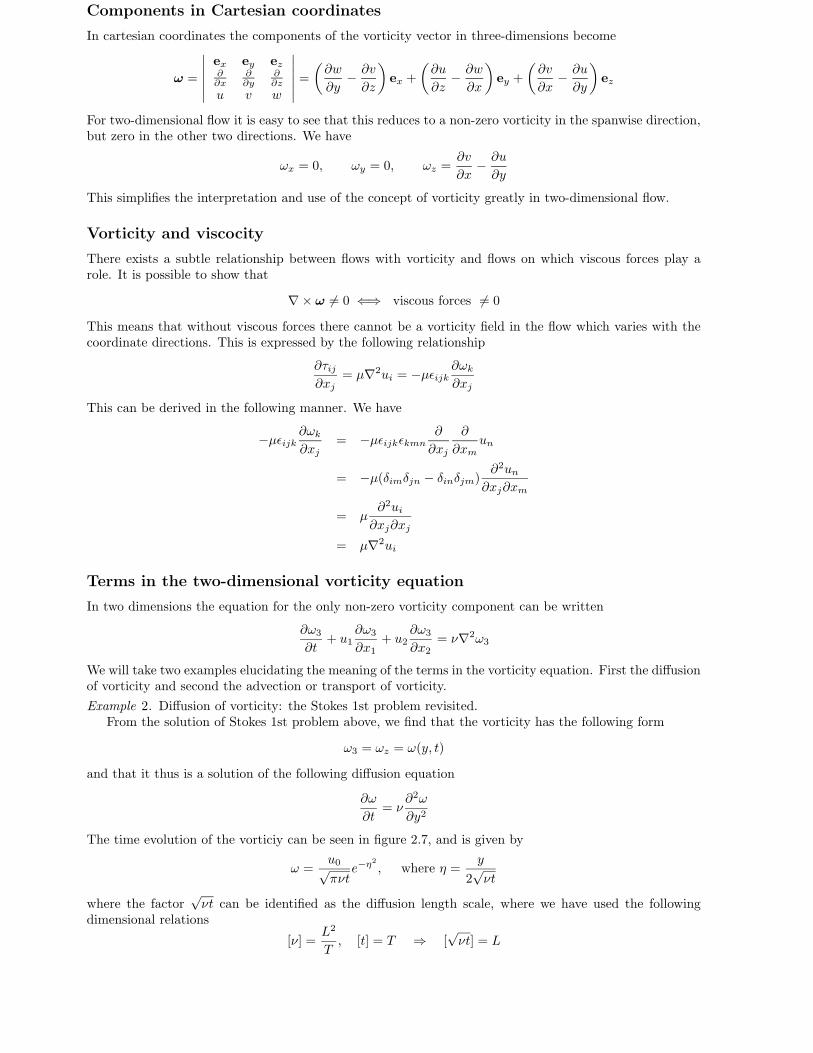
We will take two examples elucidating the meaning of the terms in the vorticity equation. First the diffusionof vorticity and second the advection or transport of vorticity.
Example 2. Diffusion of vorticity: the Stokes 1st problem revisited.From the solution of Stokes 1st problem above, we find that the vorticity has the following form
ω3 = ωz = ω(y, t)
and that it thus is a solution of the following diffusion equation
∂ω
∂t= ν
∂2ω
∂y2
The time evolution of the vorticiy can be seen in figure 2.7, and is given by
ω =u0√πνt
e−η2
, where η =y
2√νt
where the factor√νt can be identified as the diffusion length scale, where we have used the following
dimensional relations
[ν] =L2
T, [t] = T ⇒ [
√νt] = L
36 CHAPTER 2. FLOW PHYSICS
0 0.1 0.2 0.3 0.4 0.5 0.6 0.7 0.8 0.9 10
1
2
3
4
5
6
7
8
PSfrag replacements
x, x1y, x2z, x3u, u1v, u2w, u3x1x2x 0i
ri(x 0i , t
)
ui(x 0i , t
)
P(t = 0
)
xu1
u2 > u1x1x2x3x 0i
ui dtdx 0
i
dui dtri(dt)
dri(dt)
P1
P2
x1x2x3R3
R2
R1
r3
r2
r1π2 + dϕ12
V (t)S (t)
V (t+∆t)− V (t)S (t+∆t)
un
V (t+∆t)
pT0, U0
TwLT0U0
Gradient fieldswi∂p∂xi
uiDivergence free vectorfields // to boundary
Lhx1x2
p0 > p1p1undS
u · n∆txyu0p0
η = y√4νtuu0
y = η√4νt
tηy
ωz =ω(η)·u0√
πνt
t
t
y
ω
Figure 2.7: A sketch of the evolution of vorticity in Stokes 1st problem.
PSfrag replacements
x, x1y, x2z, x3u, u1v, u2w, u3x1x2x 0i
ri(x 0i , t
)
ui(x 0i , t
)
P(t = 0
)
xu1
u2 > u1x1x2x3x 0i
ui dtdx 0
i
dui dtri(dt)
dri(dt)
P1
P2
x1x2x3R3
R2
R1
r3
r2
r1π2 + dϕ12
V (t)S (t)
V (t+∆t)− V (t)S (t+∆t)
un
V (t+∆t)
pT0, U0
TwLT0U0
Gradient fieldswi∂p∂xi
uiDivergence free vectorfields // to boundary
Lhx1x2
p0 > p1p1undS
u · n∆txyu0p0
η = y√4νtuu0
y = η√4νt
tηy
ωz =ω(η)·u0√
πνt
t
x, u
v, y
︷︸︸︷
ω 6= 0
Figure 2.8: Stagnation point flow with a viscous layer close to the wall.
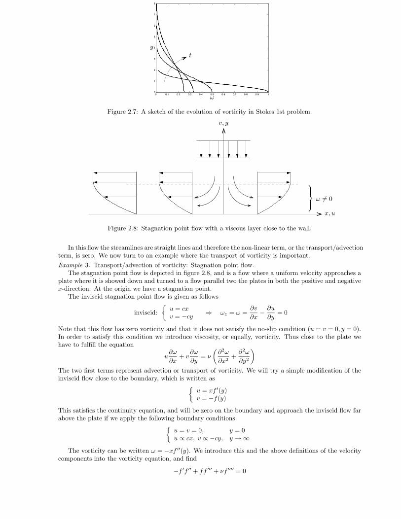
In this flow the streamlines are straight lines and therefore the non-linear term, or the transport/advectionterm, is zero. We now turn to an example where the transport of vorticity is important.
Example 3. Transport/advection of vorticity: Stagnation point flow.The stagnation point flow is depicted in figure 2.8, and is a flow where a uniform velocity approaches a
plate where it is showed down and turned to a flow parallel two the plates in both the positive and negativex-direction. At the origin we have a stagnation point.
The inviscid stagnation point flow is given as follows
inviscid:
u = cxv = −cy ⇒ ωz = ω =
∂v
∂x− ∂u
∂y= 0
Note that this flow has zero vorticity and that it does not satisfy the no-slip condition (u = v = 0, y = 0).In order to satisfy this condition we introduce viscosity, or equally, vorticity. Thus close to the plate wehave to fulfill the equation
u∂ω
∂x+ v
∂ω
∂y= ν
(∂2ω
∂x2+∂2ω
∂y2
)
The two first terms represent advection or transport of vorticity. We will try a simple modification of theinviscid flow close to the boundary, which is written as
u = xf ′(y)v = −f(y)
This satisfies the continuity equation, and will be zero on the boundary and approach the inviscid flow farabove the plate if we apply the following boundary conditions
u = v = 0, y = 0u ∝ cx, v ∝ −cy, y →∞
The vorticity can be written ω = −xf ′′(y). We introduce this and the above definitions of the velocitycomponents into the vorticity equation, and find
−f ′f ′′ + ff ′′′ + νf ′′′′ = 0

2.2. VORTICITY AND STREAMFUNCTION 37
0 1 20
0.5
1
1.5
PSfrag replacements
x, x1y, x2z, x3u, u1v, u2w, u3x1x2x 0i
ri(x 0i , t
)
ui(x 0i , t
)
P(t = 0
)
xu1
u2 > u1x1x2x3x 0i
ui dtdx 0
i
dui dtri(dt)
dri(dt)
P1
P2
x1x2x3R3
R2
R1
r3
r2
r1π2 + dϕ12
V (t)S (t)
V (t+∆t)− V (t)S (t+∆t)
un
V (t+∆t)
pT0, U0
TwLT0U0
Gradient fieldswi∂p∂xi
uiDivergence free vectorfields // to boundary
Lhx1x2
p0 > p1p1undS
u · n∆txyu0p0
η = y√4νtuu0
y = η√4νt
tηy
ωz =ω(η)·u0√
πνt
t
F, F ′, F ′′
η
F ′
F ′′
F
η
Figure 2.9: Solution to the non-dimensional equation for stagnation point flow. F is proportional to thenormal velocity, F ′ to the streamwise velocity and F ′′ to the vorticity.
The boundary conditions becomef = f ′ = 0 y = 0f ∝ cy, f ′ ∝ c, y →∞
An integral to the equation exists, which can be written
f ′2 − ff ′′ − νf ′′′ = K = evaluate y →∞ = c2
This is as far as we can come analytically and to make further numerical treatment simpler we make theequation non-dimensional with ν and c. Note that they have the dimensions
[ν] =L2
T, [c] =
1
T
and that we can use the length scale√
ν/c and the velocity scale√νc to scale the independent and the
dependent variables as
η =y
√
ν/c
F (η) =f(y)√νc
This results in the following non-dimensional equation
F ′2 − FF ′′ − F ′′′ = 1
with the boundary conditionsF = F ′ = 0, η = 0F ∝ η, η →∞
In figure 2.9 a solution of the equation is shown. It can be seen that diffusion of vorticity from the wallis balanced by transport downward by v and outward by u. The thin layer of vortical flow close to the wall
has the thickness ∼√
ν/c.
Stretching and tilting of vortex lines
In three-dimensions the vorticity is not restricted to a single non-zero component and the three-dimensionalvorticity equation governing the vorticity vector becomes
∂ωi∂t
+ uj∂ωi∂xj
︸ ︷︷ ︸
advection of vorticity
= ωj∂ui∂xj
+1
Re∇2ωi
︸ ︷︷ ︸
diffusion of vorticity

38 CHAPTER 2. FLOW PHYSICS
PSfrag replacements
x, x1y, x2z, x3u, u1v, u2w, u3x1x2x 0i
ri(x 0i , t
)
ui(x 0i , t
)
P(t = 0
)
xu1
u2 > u1x1x2x3x 0i
ui dtdx 0
i
dui dtri(dt)
dri(dt)
P1
P2
x1x2x3R3
R2
R1
r3
r2
r1π2 + dϕ12
V (t)S (t)
V (t+∆t)− V (t)S (t+∆t)
un
V (t+∆t)
pT0, U0
TwLT0U0
Gradient fieldswi∂p∂xi
uiDivergence free vectorfields // to boundary
Lhx1x2
p0 > p1p1undS
u · n∆txyu0p0
η = y√4νtuu0
y = η√4νt
tηy
ωz =ω(η)·u0√
πνt
t
C(t)
dr
Figure 2.10: A closed material curve.
The complex motion of the vorticity vector for a full three-dimensional flow can be understood by ananalogy to the equation governing the evolution of a material line, discussed in the first chapter. Theequation for a material line is
D
Dtdri = drj
∂ui∂xj
Note that if we disregard the diffusion term, i.e. the last term of the vorticity equation, the two equationsare identical. Thus we can draw the following conclusions about the development of the vortex vector
i) Stretching of vortex lines (line ‖ ω) produce ωi like stretching of dri produces length
ii) Tilting vortex lines produce ωi in one direction at expense of ωi in other direction
Helmholz and Kelvin’s theorems
The analogy with the equation for the material line directly give us a proof of Helmholz theorem. We have
Theorem 1. Helmholz theorem for inviscid flow: Vortex lines are material lines in inviscid flow.
A second theorem valid in inviscid flow is Kelvin’s theorem.
Theorem 2. Kelvin’s theorem for inviscid flow: Circulation around a material curve is constant in inviscidflow.
Proof. We show this by considering the circulation for a closed material curve, see figure 2.10,
Γm =
∮
C(t)
ui dri
We can evaluate the material time derivative of this expression with the use of Lagrangian coordinatesas follows
DΓmDt
=D
Dt
∮
C(t)
ui dri
=
Lagrange coordinatesui = ui(x
0i , t) = ui(x
0i (m), t)
ri = ri(x0i , t) = ri(x
0i (m), t)
=d
dt
∮
m
ui∂ri∂m
dm
=
∮
m
∂ui
∂t
∂ri∂m
dm+
∮
m
ui∂
∂t
(∂ri∂m
)
dm
The last term of this expression will vanish since
∮
m
ui∂
∂t
(∂ri∂m
)
dm =
∮
m
ui∂ui∂m
dm =
∮
m
∂
∂m
(1
2uiui
)
dm = 0

2.2. VORTICITY AND STREAMFUNCTION 39
PSfrag replacements
x, x1y, x2z, x3u, u1v, u2w, u3x1x2x 0i
ri(x 0i , t
)
ui(x 0i , t
)
P(t = 0
)
xu1
u2 > u1x1x2x3x 0i
ui dtdx 0
i
dui dtri(dt)
dri(dt)
P1
P2
x1x2x3R3
R2
R1
r3
r2
r1π2 + dϕ12
V (t)S (t)
V (t+∆t)− V (t)S (t+∆t)
un
V (t+∆t)
pT0, U0
TwLT0U0
Gradient fieldswi∂p∂xi
uiDivergence free vectorfields // to boundary
Lhx1x2
p0 > p1p1undS
u · n∆txyu0p0
η = y√4νtuu0
y = η√4νt
tηy
ωz =ω(η)·u0√
πνt
t
x, u
y, v
dx
dy
u = (u, v)
Figure 2.11: A streamline which is tangent to the velocity vector.
Thus we find the following resulting expression
DΓmDt
=
∮
C(t)
DuiDt
dri
=
∮
C(t)
[
− ∂p
∂xi+1
Re∇2ui
]
dri
=1
Re
∮
C(t)
∇2ui dri → 0, Re→∞
Which shows that the circulation for a material curve changes only if the viscous force 6= 0
Streamfunction
We end this section with the definition and some properties of the streamfunction. To define the stream-function we need the streamlines which are tangent to the velocity vector. In two dimensions, see figure2.11, we have
dx
dy=u
v⇐⇒ dx
u=dy
v⇐⇒ udy − v dx = 0
and in three dimensions we can writedx
u=dy
v=dz
w
For two-dimensional flow we can find the streamlines using a streamfunction. We can introduce astreamfunction ψ = ψ(x, y) with the property that the streamfunction is constant along streamlines. Wecan make the following derivation
dψ =∂ψ
∂xdx+
∂ψ
∂ydy
=
assume u =∂ψ
∂y, v = −∂ψ
∂xand check for consistency
= udy − v dx= 0, on streamlines
We can also quickly check that the definition given above satisfies continuity. We have
∂u
∂x+∂v
∂y=
∂2ψ
∂x∂y− ∂2ψ
∂y∂x= 0
Another property of the streamfunction is that the volume flux between two streamlines can be foundfrom the difference by their respective streamfunctions. We use figure 2.12 and figure 2.13 in the followingderivations of the volume flux:

40 CHAPTER 2. FLOW PHYSICS
PSfrag replacements
x, x1y, x2z, x3u, u1v, u2w, u3x1x2x 0i
ri(x 0i , t
)
ui(x 0i , t
)
P(t = 0
)
xu1
u2 > u1x1x2x3x 0i
ui dtdx 0
i
dui dtri(dt)
dri(dt)
P1
P2
x1x2x3R3
R2
R1
r3
r2
r1π2 + dϕ12
V (t)S (t)
V (t+∆t)− V (t)S (t+∆t)
un
V (t+∆t)
pT0, U0
TwLT0U0
Gradient fieldswi∂p∂xi
uiDivergence free vectorfields // to boundary
Lhx1x2
p0 > p1p1undS
u · n∆txyu0p0
η = y√4νtuu0
y = η√4νt
tηy
ωz =ω(η)·u0√
πνt
t
A
B
S
n
Ψ = ΨB
Ψ = ΨA
Figure 2.12: Integration paths between two streamlines.
PSfrag replacements
x, x1y, x2z, x3u, u1v, u2w, u3x1x2x 0i
ri(x 0i , t
)
ui(x 0i , t
)
P(t = 0
)
xu1
u2 > u1x1x2x3x 0i
ui dtdx 0
i
dui dtri(dt)
dri(dt)
P1
P2
x1x2x3R3
R2
R1
r3
r2
r1π2 + dϕ12
V (t)S (t)
V (t+∆t)− V (t)S (t+∆t)
un
V (t+∆t)
pT0, U0
TwLT0U0
Gradient fieldswi∂p∂xi
uiDivergence free vectorfields // to boundary
Lhx1x2
p0 > p1p1undS
u · n∆txyu0p0
η = y√4νtuu0
y = η√4νt
tηy
ωz =ω(η)·u0√
πνt
t
−dx
dy
ds nx
ny|n| = 1
Figure 2.13: The normal vector to a line element.
QAB =
∫ B
A
uini ds
=
∫ B
A
(nxu+ nyv) ds
=
ds
dy=1
nx, − ds
dx=1
ny
=
∫ B
A
(udy − v dx) =∫ B
A
dψ = ψB − ψA
2.3 Potential flow
Flows which can be found from the gradient of a scalar function, a so called potential, will be dealtwith in this section. Working with the velocity potential, for example, will greatly simplify calculations,but also restrict the validity of the solutions. We start with a definition of the velocity potential, thendiscuss simplifications of the momentum equations when such potentials exist, and finally we deal withtwo-dimensional potential flows, where analytic function theory can be used.
Velocity potential
Assume that the velocity can be found from a potential. In three dimensions we have
ui =∂φ
∂xior u = ∇φ
with the corresponding relations in two dimensions
u =∂φ
∂x
v =∂φ
∂y
There are several consequences of this definition of the velocity field.

2.3. POTENTIAL FLOW 41
i) Potential flow have no vorticity, which can be seen by taking the curl of the gradient of the velocitypotential, i.e.
ωi = εijk∂uk∂xj
= εijk∂2φ
∂xj∂xk= 0
ii) Potential flow is not influenced by viscous forces, which is seen by the relationship between viscousforces and vorticity, derived earlier. We have
∂τij∂xj
= µ∇2ui = −µεijk∂ωk∂xj
iii) Potential flow satisfies Laplace equation, which is a consequence of the divergence constraint appliedto the gradient of the velocity potential, i.e.
∂ui∂xi
=∂2φ
∂xi∂xi= ∇2φ = 0
Bernoulli’s equation
For potential flow the velocity field can thus be found by solving Laplace equation for the velocity potential.The momentum equations can then be used to find the pressure from the so called Bernoulli’s equation.We start by rewriting the momentum equation
∂ui∂t
+ uj∂ui∂xj
= −1ρ
∂p
∂xi+ ν∇2ui − gδi3
using the alternative form of the non-linear terms, i.e.
uj∂ui∂xj
=∂
∂xi
(1
2ukuk
)
− εijkujωk
and obtain the following equation
∂ui∂t
+∂
∂xi
(1
2ukuk +
p
ρ+ gx3
)
= εijkujωk + νεijk∂ωk∂xj
This equation can be integrated in for two different cases: potential flow (without vorticity) and sta-tionary inviscid flow with vorticity.
i) Potential flow. Introduce the definition of the velocity potential ui =∂φ∂xi
into the momentum equationabove, we have
∂
∂xi
(∂φ
∂t+1
2ukuk +
p
ρ+ gx3
)
= 0 ⇒
∂φ
∂t+1
2(u21 + u
22 + u
23) +
p
ρ+ gx3 = f(t)
ii) Stationary, inviscid flow with vorticity. Integrate the momentum equations along a streamline, seefigure 2.14. We have
∫
ti∂
∂xi
(1
2ukuk +
p
ρ+ gx3
)
ds =
∫
εijkuiuujωk ds = 0 ⇒
1
2(u21 + u
22 + u
23) +
p
ρ+ gx3 = constant along streamlines
Thus, Bernoulli’s equation can be used to calculate the pressure when the velocity is known, for twodifferent flow situations.
Example 4. Ideal vortex: Swirling stationary flow without vorticity. The velocity potential u = ∇φ inpolar coordinates can be written
ur =∂φ
∂r
uθ =1
r
∂φ
∂θ

42 CHAPTER 2. FLOW PHYSICS
PSfrag replacements
x, x1y, x2z, x3u, u1v, u2w, u3x1x2x 0i
ri(x 0i , t
)
ui(x 0i , t
)
P(t = 0
)
xu1
u2 > u1x1x2x3x 0i
ui dtdx 0
i
dui dtri(dt)
dri(dt)
P1
P2
x1x2x3R3
R2
R1
r3
r2
r1π2 + dϕ12
V (t)S (t)
V (t+∆t)− V (t)S (t+∆t)
un
V (t+∆t)
pT0, U0
TwLT0U0
Gradient fieldswi∂p∂xi
uiDivergence free vectorfields // to boundary
Lhx1x2
p0 > p1p1undS
u · n∆txyu0p0
η = y√4νtuu0
y = η√4νt
tηy
ωz =ω(η)·u0√
πνt
t
u
t = uu
Figure 2.14: Integration of the momentum equation along a streamline.
PSfrag replacements
x, x1y, x2z, x3u, u1v, u2w, u3x1x2x 0i
ri(x 0i , t
)
ui(x 0i , t
)
P(t = 0
)
xu1
u2 > u1x1x2x3x 0i
ui dtdx 0
i
dui dtri(dt)
dri(dt)
P1
P2
x1x2x3R3
R2
R1
r3
r2
r1π2 + dϕ12
V (t)S (t)
V (t+∆t)− V (t)S (t+∆t)
un
V (t+∆t)
pT0, U0
TwLT0U0
Gradient fieldswi∂p∂xi
uiDivergence free vectorfields // to boundary
Lhx1x2
p0 > p1p1undS
u · n∆txyu0p0
η = y√4νtuu0
y = η√4νt
tηy
ωz =ω(η)·u0√
πνt
t
r
Figure 2.15: Streamlines for the ideal vortex.
The velocity potential satisfies Laplace equation, which in polar coordinates becomes
∇2φ =1
r
∂
∂r
(1
r
∂φ
∂r
)
+1
r
∂2φ
∂θ2= 0
The first term vanishes since ∂φ∂r = ur = 0. Integrate the resulting equation twice and we find
φ = Cθ +D
The constant D is arbitrary so we can set it to zero. Using the definition of the circulation we find
uθ =C
r, C =
Γ
2π
We can easily find the streamfunction for this flow. In polar coordinates the streamfunction is defined
ur =1
r
∂ψ
∂θ
uθ = −∂ψ∂r
Note that the streamfunction satisfies continuity, i.e. ∇ · u = 0. We use the solution from the velocitypotential to find the streamfunction, we have
∂ψ
∂r= − Γ
2πr⇒ ψ = − Γ
2πln r
The streamfunction is constant along streamlines resulting in circular streamlines, see figure 2.15We can now use Bernoulli’s equation to calculate the pressure distribution for the ideal vortex as
1
2u2θ + p = p∞ ⇒ p = p∞ −
Γ2
8π2r2
Note that the solution has a singularity at the origin.
Two-dimensional potential flow using analytic functions
For two-dimensional flows we can use analytic function theory, i.e. complex valued functions, to calculatethe velocity potential. In fact, as we will show in the following. Any analytic function represents a two-dimensional potential flow.

2.3. POTENTIAL FLOW 43
We start by showing that both the velocity potential and the streamfunciton satisfy Laplace equation.Velocity potential φ for two-dimensional flow is defined
u =∂φ
∂x
v =∂φ
∂y
Using the continuity equation gives∂u
∂x+∂v
∂y= ∇2φ = 0
The streamfunction ψ is defined
u =∂ψ
∂y
v = −∂ψ∂x
By noting that potential flow has no vorticity we find
−ω = −∂v∂x
+∂y
∂y= ∇2ψ = 0
Thus, both the velocity potential φ and the streamfunction ψ satisfy Laplace equation.We can utilize analytic function theory by introducing the complex function
F (z) = φ(x, y) + iψ(x, y)
wherez = x+ iy = reiθ = r(cos θ + i sin θ)
which will be denoted the complex potential.We now recall some useful results from analytic function theory.
F ′(z) exists and is unique ⇐⇒ F (z) is an analytic function
The fact that a derivative of a complex function should be unique rests on the validity of the Cauchy–Riemann equations. We can derive those equations by requiring that a derivative of a complex functionshould be the same independent of the direction we take the limit in the complex plane, see figure 2.16.We have
F ′(z) = lim∆z→0
1
∆z[F (z +∆z)− F (z)]
= lim∆x→0
1
∆x[φ(x+∆x, y)− φ(x, y) + iψ(x+∆x, y)− iψ(x, y)]
= limi∆y→0
1
i∆y[φ(x, y +∆y)− φ(x, y) + iψ(x, y +∆y)− iψ(x, y)]
⇒
∂φ
∂x=∂ψ
∂yreal part
i∂ψ
∂x=1
i
∂φ
∂y⇒ ∂ψ
∂x= −∂φ
∂yimaginary part
Thus we have the Cauchy–Riemann equations as a necessary requirement for a complex function to beanalytic, i.e.
∂φ
∂x=∂ψ
∂yand
∂φ
∂y= −∂ψ
∂x
Using the Cauchy-Riemann equations we can show that the real φ and imaginary part ψ of the complexpotential satisfy Laplace equations and thus that they are candidates for identification with the velocitypotential and streamfunction of a two-dimensional potential flow. We have
∂2φ
∂x2=
∂
∂x
(∂ψ
∂y
)
=∂
∂y
(∂ψ
∂x
)
= −∂2φ
∂y2
∂2ψ
∂y2=
∂
∂y
(∂φ
∂x
)
=∂
∂x
(∂φ
∂y
)
= −∂2ψ
∂x2

44 CHAPTER 2. FLOW PHYSICS
PSfrag replacements
x, x1y, x2z, x3u, u1v, u2w, u3x1x2x 0i
ri(x 0i , t
)
ui(x 0i , t
)
P(t = 0
)
xu1
u2 > u1x1x2x3x 0i
ui dtdx 0
i
dui dtri(dt)
dri(dt)
P1
P2
x1x2x3R3
R2
R1
r3
r2
r1π2 + dϕ12
V (t)S (t)
V (t+∆t)− V (t)S (t+∆t)
un
V (t+∆t)
pT0, U0
TwLT0U0
Gradient fieldswi∂p∂xi
uiDivergence free vectorfields // to boundary
Lhx1x2
p0 > p1p1undS
u · n∆txyu0p0
η = y√4νtuu0
y = η√4νt
tηy
ωz =ω(η)·u0√
πνt
tx
iy
︸ ︷︷ ︸
∆x
︸︷︷︸
i∆y
Figure 2.16: The complex plane and the definitions of analytic functions.
In addition to satisfying the Laplace equations, we also have to show that the Cauchy-Riemann equationsare consistent with the definition of the velocity potential and the streamfunciton. The Cauchy–Riemannequations are
u =∂φ
∂x=∂ψ
∂y
v =∂φ
∂y= −∂ψ
∂x
which recovers the definitions of the velocity potential and the streamfunction. Thus any analytic complexfunction can be identified with a potential flow, where the real part is the velocity potential and theimaginary part is the streamfunction.
We can now define the complex velocity as the complex conjugate of the velocity vector since
W (z) =dF
dz=∂φ
∂x+ i
∂ψ
∂x= u− iv
It will be useful to have a similar relation for polar coordinates, see figure 2.17. In this case we have
u = ur cos θ − uθ sin θv = ur sin θ + uθ cos θ
W (z) = u− iv = [ur(r, θ)− iuθ(r, θ)] e−iθ︸︷︷︸
cos θ−i sin θ
We will now take several examples of how potential velocity fields can be found from analytic functions.
Example 5. Calculate the velocity field from the complex potential F = Ue−iαz. The complex velocitybecomes
W (z) = F ′ = Ue−iα = U cosα− i sinαwhich gives us the solution for the velocity field in physical variables, see figure 2.18, as
u = U cosαv = U sinα
Example 6. Calculate the velocity field from the complex potential F = Azn. In polar coordinates thecomplex potential becomes
Arneinθ = Arn cos(nθ) + iArn sin(nθ)
Thus the velocity potential and the streamfunction can be identified as
φ = Arn cos(nθ)ψ = Arn sin(nθ)

2.3. POTENTIAL FLOW 45
PSfrag replacements
x, x1y, x2z, x3u, u1v, u2w, u3x1x2x 0i
ri(x 0i , t
)
ui(x 0i , t
)
P(t = 0
)
xu1
u2 > u1x1x2x3x 0i
ui dtdx 0
i
dui dtri(dt)
dri(dt)
P1
P2
x1x2x3R3
R2
R1
r3
r2
r1π2 + dϕ12
V (t)S (t)
V (t+∆t)− V (t)S (t+∆t)
un
V (t+∆t)
pT0, U0
TwLT0U0
Gradient fieldswi∂p∂xi
uiDivergence free vectorfields // to boundary
Lhx1x2
p0 > p1p1undS
u · n∆txyu0p0
η = y√4νtuu0
y = η√4νt
tηy
ωz =ω(η)·u0√
πνt
t
x
y
r
θ
u
v
ur
uθ
u
Figure 2.17: The definition of polar coordinates.
PSfrag replacements
x, x1y, x2z, x3u, u1v, u2w, u3x1x2x 0i
ri(x 0i , t
)
ui(x 0i , t
)
P(t = 0
)
xu1
u2 > u1x1x2x3x 0i
ui dtdx 0
i
dui dtri(dt)
dri(dt)
P1
P2
x1x2x3R3
R2
R1
r3
r2
r1π2 + dϕ12
V (t)S (t)
V (t+∆t)− V (t)S (t+∆t)
un
V (t+∆t)
pT0, U0
TwLT0U0
Gradient fieldswi∂p∂xi
uiDivergence free vectorfields // to boundary
Lhx1x2
p0 > p1p1undS
u · n∆txyu0p0
η = y√4νtuu0
y = η√4νt
tηy
ωz =ω(η)·u0√
πνt
t
α
Figure 2.18: Constant velocity at an angle α.

46 CHAPTER 2. FLOW PHYSICS
PSfrag replacements
x, x1y, x2z, x3u, u1v, u2w, u3x1x2x 0i
ri(x 0i , t
)
ui(x 0i , t
)
P(t = 0
)
xu1
u2 > u1x1x2x3x 0i
ui dtdx 0
i
dui dtri(dt)
dri(dt)
P1
P2
x1x2x3R3
R2
R1
r3
r2
r1π2 + dϕ12
V (t)S (t)
V (t+∆t)− V (t)S (t+∆t)
un
V (t+∆t)
pT0, U0
TwLT0U0
Gradient fieldswi∂p∂xi
uiDivergence free vectorfields // to boundary
Lhx1x2
p0 > p1p1undS
u · n∆txyu0p0
η = y√4νtuu0
y = η√4νt
tηy
ωz =ω(η)·u0√
πνt
t
Ψ = 0
Ψ = 0
Ψ = 0
πn
Figure 2.19: Flow towards a corner.
PSfrag replacements
x, x1y, x2z, x3u, u1v, u2w, u3x1x2x 0i
ri(x 0i , t
)
ui(x 0i , t
)
P(t = 0
)
xu1
u2 > u1x1x2x3x 0i
ui dtdx 0
i
dui dtri(dt)
dri(dt)
P1
P2
x1x2x3R3
R2
R1
r3
r2
r1π2 + dϕ12
V (t)S (t)
V (t+∆t)− V (t)S (t+∆t)
un
V (t+∆t)
pT0, U0
TwLT0U0
Gradient fieldswi∂p∂xi
uiDivergence free vectorfields // to boundary
Lhx1x2
p0 > p1p1undS
u · n∆txyu0p0
η = y√4νtuu0
y = η√4νt
tηy
ωz =ω(η)·u0√
πνt
t Ψ = 0
Figure 2.20: Uniform flow over a flat plate.
and we can calculate the complex velocity as
W (z) = F ′ = nAzn−1
= nArn−1einθe−iθ
= nArn−1[cos(nθ) + i sin(nθ)]e−iθ
This gives us the solution for the velocity in polar coordinates asur = nArn−1 cos(nθ)uθ = −nArn−1 sin(nθ)
This is a flow which approaches a corner, see figure 2.19. The streamfunction is zero on the walls and onthe stagnation point streamline. By solving for the zero streamlines we can calculate the angle between awall aligned with the x-axis and the stagnation point streamline. We have
ψ = Arn sin(nθ) = 0 ⇒ θ =πk
n
Figure 2.20 shows the uniform flow over a flat plate which results when n = 1.Figure 2.21 shows the stagnation point flow when n = 2. Here the analysis can be done in Cartesian
coordinates
F = Az2
W (z) = F ′ = 2Az
= 2A(x+ iy)
⇒u = 2Axv = −2Ay
Figure 2.22 shows the flow towards a wedge when 1 ≤ n ≤ 2. The velocity along the wedge edge (x axisin figure 2.22) is
ur = nArn−1 cos(nθ)⇒ θ = 0 ⇒ u = ur = nArn−1 = Cxn−1
The wedge angle is
ϕ = 2π − 2πn= 2π
n− 1n
PSfrag replacements
x, x1y, x2z, x3u, u1v, u2w, u3x1x2x 0i
ri(x 0i , t
)
ui(x 0i , t
)
P(t = 0
)
xu1
u2 > u1x1x2x3x 0i
ui dtdx 0
i
dui dtri(dt)
dri(dt)
P1
P2
x1x2x3R3
R2
R1
r3
r2
r1π2 + dϕ12
V (t)S (t)
V (t+∆t)− V (t)S (t+∆t)
un
V (t+∆t)
pT0, U0
TwLT0U0
Gradient fieldswi∂p∂xi
uiDivergence free vectorfields // to boundary
Lhx1x2
p0 > p1p1undS
u · n∆txyu0p0
η = y√4νtuu0
y = η√4νt
tηy
ωz =ω(η)·u0√
πνt
t
Figure 2.21: Stagnation point flow when n = 2.

2.3. POTENTIAL FLOW 47
PSfrag replacements
x, x1y, x2z, x3u, u1v, u2w, u3x1x2x 0i
ri(x 0i , t
)
ui(x 0i , t
)
P(t = 0
)
xu1
u2 > u1x1x2x3x 0i
ui dtdx 0
i
dui dtri(dt)
dri(dt)
P1
P2
x1x2x3R3
R2
R1
r3
r2
r1π2 + dϕ12
V (t)S (t)
V (t+∆t)− V (t)S (t+∆t)
un
V (t+∆t)
pT0, U0
TwLT0U0
Gradient fieldswi∂p∂xi
uiDivergence free vectorfields // to boundary
Lhx1x2
p0 > p1p1undS
u · n∆txyu0p0
η = y√4νtuu0
y = η√4νt
tηy
ωz =ω(η)·u0√
πνt
t
ϕ
Figure 2.22: The flow over a wedge when 1 ≤ n ≤ 2.
PSfrag replacements
x, x1y, x2z, x3u, u1v, u2w, u3x1x2x 0i
ri(x 0i , t
)
ui(x 0i , t
)
P(t = 0
)
xu1
u2 > u1x1x2x3x 0i
ui dtdx 0
i
dui dtri(dt)
dri(dt)
P1
P2
x1x2x3R3
R2
R1
r3
r2
r1π2 + dϕ12
V (t)S (t)
V (t+∆t)− V (t)S (t+∆t)
un
V (t+∆t)
pT0, U0
TwLT0U0
Gradient fieldswi∂p∂xi
uiDivergence free vectorfields // to boundary
Lhx1x2
p0 > p1p1undS
u · n∆txyu0p0
η = y√4νtuu0
y = η√4νt
tηy
ωz =ω(η)·u0√
πνt
t
Figure 2.23: Line source.
We now list several other examples of potential flow fields obtained from analytic functions.
Example 7. Line source.
F (z) =m
2πln z
=m
2πln(reiθ)
=m
2π[ln r + iθ]
The velocity potential and the streamfunction become
φ =m
2πln r
ψ =m
2πθ
The complex velocity can be written as
W (z) = F ′ =m
2πz=
m
2πre−iθ
which gives the solution in polar coordinates, see figure 2.23, as
ur =m
2πr
uθ = 0
We can now calculate the volume flux from the source as
Q =
∫ 2π
0
m
2πrr dθ = m
Example 8. Line vortex.
F (z) = −i Γ2πln z
=Γ
2π[θ − i ln r]

48 CHAPTER 2. FLOW PHYSICS
PSfrag replacements
x, x1y, x2z, x3u, u1v, u2w, u3x1x2x 0i
ri(x 0i , t
)
ui(x 0i , t
)
P(t = 0
)
xu1
u2 > u1x1x2x3x 0i
ui dtdx 0
i
dui dtri(dt)
dri(dt)
P1
P2
x1x2x3R3
R2
R1
r3
r2
r1π2 + dϕ12
V (t)S (t)
V (t+∆t)− V (t)S (t+∆t)
un
V (t+∆t)
pT0, U0
TwLT0U0
Gradient fieldswi∂p∂xi
uiDivergence free vectorfields // to boundary
Lhx1x2
p0 > p1p1undS
u · n∆txyu0p0
η = y√4νtuu0
y = η√4νt
tηy
ωz =ω(η)·u0√
πνt
t
Figure 2.24: Ideal vortex.
The velocity potential and the streamfunction become
φ =Γ
2πθ
ψ = − Γ
2πln r
The complex velocity can be written as
W (z) = F ′ = −i Γ2πr
e−iθ
which gives the solution in polar coordinates, see figure 2.24, as
ur = 0
uθ =Γ
2πr
Example 9. The dipole has the complex potential
F (z) =mε
πz
Example 10. The potential flow around a cylinder has the complex potential
F (z) = Uz + Ur20z
Example 11. The potential flow around a cylinder with circulation has the complex potential
F (z) = Uz + Ur20z− i Γ2πln
z
r0
Example 12. Airfoils. The inviscid flow around some airfoils can be calculated with conformal mappingsof solutions from cylinder with circulation.
2.4 Boundary layers
For flows with high Reynolds number Re, where the viscous effects are small, most of the flow can beconsidered inviscid and a simpler set of equations, the Euler equations, can be solved. The Euler equationsare obtained if Re → ∞ in the Navier-Stokes equations. However, the highest derivatives are present inthe viscous terms, thus a smaller number of boundary conditions can be satisfied when solving the Eulerequations. In particular, the no flow condition can be satisfied at a solid wall but not the no slip condition.In order to satisfy the no slip condition we need to add the viscous term. Thus, there will be a layer closeto the solid walls where the viscous terms are important even for very high Reynolds number flow. Thislayer will be very thin and the flow in that region is called boundary layer flow.

2.4. BOUNDARY LAYERS 49
PSfrag replacements
x, x1y, x2z, x3u, u1v, u2w, u3x1x2x 0i
ri(x 0i , t
)
ui(x 0i , t
)
P(t = 0
)
xu1
u2 > u1x1x2x3x 0i
ui dtdx 0
i
dui dtri(dt)
dri(dt)
P1
P2
x1x2x3R3
R2
R1
r3
r2
r1π2 + dϕ12
V (t)S (t)
V (t+∆t)− V (t)S (t+∆t)
un
V (t+∆t)
pT0, U0
TwLT0U0
Gradient fieldswi∂p∂xi
uiDivergence free vectorfields // to boundary
Lhx1x2
p0 > p1p1undS
u · n∆txyu0p0
η = y√4νtuu0
y = η√4νt
tηy
ωz =ω(η)·u0√
πνt
t
L
δω ≈ 0U →
Figure 2.25: Estimate of the viscous region for an inviscid vorticity free inflow in a plane channel.
PSfrag replacements
x, x1y, x2z, x3u, u1v, u2w, u3x1x2x 0i
ri(x 0i , t
)
ui(x 0i , t
)
P(t = 0
)
xu1
u2 > u1x1x2x3x 0i
ui dtdx 0
i
dui dtri(dt)
dri(dt)
P1
P2
x1x2x3R3
R2
R1
r3
r2
r1π2 + dϕ12
V (t)S (t)
V (t+∆t)− V (t)S (t+∆t)
un
V (t+∆t)
pT0, U0
TwLT0U0
Gradient fieldswi∂p∂xi
uiDivergence free vectorfields // to boundary
Lhx1x2
p0 > p1p1undS
u · n∆txyu0p0
η = y√4νtuu0
y = η√4νt
tηy
ωz =ω(η)·u0√
πνt
tLδ
ω ≈ 0U →
y, v
x, uL
U
δ
Figure 2.26: Boundary layer profile close to a solid wall.
We begin this section by estimating the thickness of the viscous region in channel with inviscid inflow(zero vorticity), see figure 2.25.
By analogy to the Stokes solution for the instantaneously starting plate, we can estimate the distancethe vorticity has diffused from the wall toward the channel centerline as δ ∼ √νts. Where ts is time of afluid particle with velocity U has travelled length L, i.e. ts =
L
U. Thus we can estimate δ/L as
⇒ δ
L=
√νtsL
=1
L
(νL
U
)1/2
=( ν
UL
)1/2
=1√Re
→ 0 as Re→∞
We will now divide the flow into a central/outer inviscid part and a boundary layer part close to walls,where the no slip condition is fulfilled. Since we expect this region to be thin for high Reynolds numbers,we expect large velocity gradients near walls.
We choose different length scales inside boundary layer and in inviscid region as indicated in figure 2.26,as
Inviscid : U velocity scale for u, v: L length scale for x, y
BL : U velocity scale for u: α velocity scale for v: L length scale for x: δ length scale for y
The pressure scale is assumed to be ρU 2 for both the inner and the outer region. The unknown velocityscale for the normal velocity α is determined using continuity
∂u
∂x︸︷︷︸
O
U
L
+∂v
∂y︸︷︷︸
O[α
δ
]
= 0
which implies that
U
L=α
δ⇒ α =
δ
LU
In this manner both terms in the continuity equation have the same size.
Let us use these scalings in the steady momentum equations and disregard small terms. We obtain thefollowing estimates for the size of the terms in the normal momentum equation

50 CHAPTER 2. FLOW PHYSICS
↑ y : u∂v
∂x+ v
∂v
∂y= −1
ρ
∂p
∂y+ ν
∂2v
∂x2+ ν
∂2v
∂y2
U · 1L
δU
L
δU
L· 1δ· δUL
U2
δνL2 · δUL
ν
δ2δU
L(δ
L
)2 (δ
L
)2
11
Re
(δ
L
)21
Re
where the last line was obtained by dividing all the terms on the second line by U 2/δ. When R → ∞and δ/L is small, only pressure term O(1), which implies that
∂p
∂y= 0 ⇒ p = p(x)
Thus, the pressure is constant through the boundary layer, given by the inviscid outer solution.Next we estimate the size of the terms in the streamwise momentum equation as
→ x : u∂u
∂x+ v
∂u
∂y= −1
ρ
∂p
∂x+ ν
∂2u
∂x2+ ν
∂2u
∂y2
U2
L
δU
L· Uδ
U2
L
ν
L2· U ν
δ2U
1 1 11
Re
1
Re·(L
δ
)2
The first three terms are order one and the fourth term negligible when the Reynolds number becomelarge. In order to keep the last term, the only choice that gives a consistent approximation, we have toassume that
δ
L∼ 1√
Re
which is the same estimate as we found for the extent of the boundary layer in the channel inflow case.Thus we are left with the parabolic equation in x since the second derivative term in that direction isneglected. We have
u∂u
∂x+ v
∂u
∂y= −1
ρ
∂p
∂x+ ν
∂2u
∂y2
In summary, the steady boundary layer equations for two-dimensional flow is
u∂u
∂x+ v
∂u
∂y= −1
ρ
∂p
∂x+ ν
∂2u
∂y2∂u
∂x+∂v
∂y= 0
with the initial (IC) and boundary conditions (BC)IC : u (x = x0, y) = uin (y)
BC : u (x, y = 0) = 0v (x, y = 0) = 0u (x, y →∞) = ue (x) outer inviscid flow
where the initial condition is at x = x0 and the equations are marched in the downstream direction.There are several things to note about these equations.
First, vin cannot be given as its own initial condition. By using continuity one can show that once theu0 is given the momentum equation can be written in the form
−∂v∂y+ f (y) v = g (y)
which can be integrated in the y-direction to give the initial normal velocity.Second, the system of equations is a third order system in y and thus only three boundary conditions
can be enforced. We have the no flow and the no slip conditions at the wall and the u = ue in the freestream. Thus no boundary condition for v in the free stream can be given.

2.4. BOUNDARY LAYERS 51
PSfrag replacements
x, x1y, x2z, x3u, u1v, u2w, u3x1x2x 0i
ri(x 0i , t
)
ui(x 0i , t
)
P(t = 0
)
xu1
u2 > u1x1x2x3x 0i
ui dtdx 0
i
dui dtri(dt)
dri(dt)
P1
P2
x1x2x3R3
R2
R1
r3
r2
r1π2 + dϕ12
V (t)S (t)
V (t+∆t)− V (t)S (t+∆t)
un
V (t+∆t)
pT0, U0
TwLT0U0
Gradient fieldswi∂p∂xi
uiDivergence free vectorfields // to boundary
Lhx1x2
p0 > p1p1undS
u · n∆txyu0p0
η = y√4νtuu0
y = η√4νt
tηy
ωz =ω(η)·u0√
πνt
tLδ
ω ≈ 0U →y, vx, u
LUδ
u0u0
Figure 2.27: Boundary layer flow over a flat plate with zero pressure gradient.
Third, ue(x) = uinv(x, y = 0), i.e. the boundary layer solution in the free stream approaches the inviscidsolution evaluated at the wall, since the thickness of the boundary layer is zero from the inviscid point ofview.
Fourth, the pressure gradient term in the momentum equation can be written in terms of the edgevelocity ue using the Bernoulli equation. We have
p (x) +1
2ρu2e (x) = const
which implies that
−1ρ
dp
dx= ue
duedx
Blasius flow over flat plate
Consider the boundary layer equations for a flow over a flat plate with zero pressure gradient, i.e. the outerinviscid flow is ue (x) = u0. The boundary layer equations become
u∂u
∂x+ v
∂u
∂y= ν
∂2u
∂y2∂u
∂x+∂v
∂y= 0
IC : u (x = x0, y) = u0
BC : u (x, y = 0) = 0v (x, y = 0) = 0u (x, y →∞) = u0
We introduce the two-dimensional stream function Ψ
u =∂Ψ
∂y, v = −∂Ψ
∂x
which implicitly satisfies continuity. The boundary layer equations become
∂Ψ
∂y· ∂
2Ψ
∂x∂y− ∂Ψ
∂x· ∂
2Ψ
∂y2= ν
∂3Ψ
∂y3
with appropriate initial and boundary conditions.
Similarity solution
We will now look for a similarity solution. Let
u =∂Ψ
∂y= u0f
′ (η) , η =y
δ (x)
which by integration in the y-direction implies
Ψ (x, y) = u0δ (x) f (η)
We can now evaluate the various terms in the momentum equation. We give two below
v = −∂Ψ∂x
= −u0(
δ′f + δf ′∂η
∂x
)
= −u0(
δ′f − y
δf ′δ′
)
= u0 (ηf′ − f) δ′

52 CHAPTER 2. FLOW PHYSICS
0 0.2 0.4 0.6 0.8 10
1
2
3
4
5
PSfrag replacements
x, x1y, x2z, x3u, u1v, u2w, u3x1x2x 0i
ri(x 0i , t
)
ui(x 0i , t
)
P(t = 0
)
xu1
u2 > u1x1x2x3x 0i
ui dtdx 0
i
dui dtri(dt)
dri(dt)
P1
P2
x1x2x3R3
R2
R1
r3
r2
r1π2 + dϕ12
V (t)S (t)
V (t+∆t)− V (t)S (t+∆t)
un
V (t+∆t)
pT0, U0
TwLT0U0
Gradient fieldswi∂p∂xi
uiDivergence free vectorfields // to boundary
Lhx1x2
p0 > p1p1undS
u · n∆txyu0p0
η = y√4νtuu0
y = η√4νt
tηy
ωz =ω(η)·u0√
πνt
tLδ
ω ≈ 0U →y, vx, u
LUδu0
η = y√νx/u0
f ′ = uu0
Blasius profile
Figure 2.28: Similarity solution giving the Blasius boundary layer profile.
∂2Ψ
∂x∂y= −u0f ′′
η
δδ′
If these and the other corresponding terms are introduced into the momentum equation we have thefollowing equation for f
−u20f ′f ′′η
δδ′ + u20 (ηf
′ − f) f′′δ′
δ= νu0
f ′′′
δ2
which can be simplified to
f ′′′ +u0δδ
′
νff ′′ = 0
For a similarity solution to be possible, the coefficient in front of the ff ′′ term has to be constant. Thisimplies
u0δδ′
ν=1
2⇒
∫
δδ′ dx =1
2
∫ν dx
u0⇒ 1
2δ2 =
1
2
νx
u0
which implies that δ (x) =
√νx
u0, where we have chosen the constant of integration such that δ = 0
when x = 0. We are left with the Blasius equation and boundary conditions
f ′′′ +1
2ff ′′ = 0
BC :
f (0) = f ′ (0) = 0f ′ (∞) = 1
The numerical solution to the Blasius equation gives the self-similar velocity profile seen in figure 2.28.The boundary layer thickness can be evaluated as the height where the velocity has reached 99% of the
free stream value. We have
f ′ (η99) = 0.99 ⇒ η99 =δ99√
νxu0
= 4.9 ⇒ δ99 = 4.9
√νx
u0
where it can be seen that the boundary layer thickness grows as√x.
Displacement thickness and skin friction coefficient
Another measure of the boundary layer thickness is the displacement δ∗ of the wall needed in order to havethe same volume flux of the inviscid flow as for the flow in the boundary layer. With the help of figure 2.29we can evaluate this as
∫ y0
0
udy ≡∫ y
δ∗u0 dy =
∫ y
0
u0 dy − δ∗u0
which implies that

2.4. BOUNDARY LAYERS 53
PSfrag replacements
x, x1y, x2z, x3u, u1v, u2w, u3x1x2x 0i
ri(x 0i , t
)
ui(x 0i , t
)
P(t = 0
)
xu1
u2 > u1x1x2x3x 0i
ui dtdx 0
i
dui dtri(dt)
dri(dt)
P1
P2
x1x2x3R3
R2
R1
r3
r2
r1π2 + dϕ12
V (t)S (t)
V (t+∆t)− V (t)S (t+∆t)
un
V (t+∆t)
pT0, U0
TwLT0U0
Gradient fieldswi∂p∂xi
uiDivergence free vectorfields // to boundary
Lhx1x2
p0 > p1p1undS
u · n∆txyu0p0
η = y√4νtuu0
y = η√4νt
tηy
ωz =ω(η)·u0√
πνt
tLδ
ω ≈ 0U →y, vx, u
LUδu0
η = y√νx/u0
f ′ = uu0
Blasius profileδ∗
Figure 2.29: The displacement thickness δ∗
PSfrag replacements
x, x1y, x2z, x3u, u1v, u2w, u3x1x2x 0i
ri(x 0i , t
)
ui(x 0i , t
)
P(t = 0
)
xu1
u2 > u1x1x2x3x 0i
ui dtdx 0
i
dui dtri(dt)
dri(dt)
P1
P2
x1x2x3R3
R2
R1
r3
r2
r1π2 + dϕ12
V (t)S (t)
V (t+∆t)− V (t)S (t+∆t)
un
V (t+∆t)
pT0, U0
TwLT0U0
Gradient fieldswi∂p∂xi
uiDivergence free vectorfields // to boundary
Lhx1x2
p0 > p1p1undS
u · n∆txyu0p0
η = y√4νtuu0
y = η√4νt
tηy
ωz =ω(η)·u0√
πνt
tLδ
ω ≈ 0U →y, vx, u
LUδu0
η = y√νx/u0
f ′ = uu0
Blasius profile
δ∗x
Separation point
⇐= Pressure force
Figure 2.30: Boundary layer separation caused by a pressure force directed upstream, a so called adversepressure gradient.
δ∗ =
∫ ∞
0
(
1− u
u0
)
dy =
√νx
u0
∫ ∞
0
[1− f ′ (η)] dη
If we evaluate this expression for the Blasius boundary layer we have δ∗ = 1.72√
νxu0.
A quantity which is of large importance in practical applications is the skin friction coefficient. Theskin friction at the wall is
τw = µ∂u
∂y
∣∣∣y=0
=µu0δf ′′ (0) =
ρu20√
u0xν
f ′′ (0) =0.332ρu20√
Rex
where the last term is the expression evaluated for Blasius flow. This can be used to evaluate the skinfriction coefficient as
Cf =τw12ρu
20
=0.664√Rex
where the last terms again is the Blasius value.
Boundary layer separation
A large adverse pressure gradient(∂p∂x > 0
)
may cause a back flow region close to wall, see figure 2.30.
The boundary layer equations cannot be integrated past a point of separation, since they becomesingular at that point. This can be seen from the following manipulations of the boundary layer equations.If we take the momentum equation
u∂u
∂x+ v
∂u
∂y= −1
ρ
dp
dx+ ν
∂2u
∂y2
take the normal derivative and use continuity we have
u∂2u
∂x∂y+ v
∂2u
∂y2= ν
∂3u
∂y3
If we again take the normal derivative and use continuity we can write this as
1
2
∂
∂x
(∂u
∂y
)2
+ u∂3u
∂x∂y2− ∂u
∂x
∂2u
∂y2+ v
∂3u
∂y3= ν
∂4u
∂y4
This expression evaluated at the wall, with the use of the boundary conditions, become

54 CHAPTER 2. FLOW PHYSICS
1
2
∂
∂x
(
∂u
∂y
∣∣∣∣y=0
)2
= ν∂4u
∂y4
∣∣∣∣y=0
︸ ︷︷ ︸
±κ2
which can be integrated to yield
(
∂u
∂y
∣∣∣∣y=0
)2
= ±κ2x+ C
At the point of separation x = xs, i.e. where
(
∂u∂y
∣∣∣∣y=0
= 0
)
this expression is
∂u
∂y
∣∣∣∣y=0
= κ√xs − x
We can see that the boundary layer equations are not valid beyond point of separation since we havea square root singularity at that point. In addition, the point of separation is the limiting point afterwhich there is back flow close to the wall. This means that there is information propagating upstream,invalidating the downstream parabolic nature of the equations assumed by the downstream integration ofthe equations.
In practical situations it is very important to be able to predict the point of separation, for examplewhen an airfoil stalls and experience a severe loss of lift.
2.5 Turbulent flow
Reynolds average equations
Turbulent flow is inherently time dependent and chaotic. However, in applications one is not usuallyinterested in knowing full the details of this flow, but rather satisfied with the influence of the turbulenceon the averaged flow. For this purpose we define an ensemble average as
Ui = ui = limN→∞
1
N
N∑
n=1
u(n)i
where each member of the ensemble u(n)i is regarded as an independent realization of the flow.
We are now going to derive an equation governing the mean flow Ui. Divide the total flow into anaverage and a fluctuating component u′i as
ui = ui + u′i p = p+ p′
and introduce into the Navier-Stokes equations. We find
∂u′i∂t
+∂ui∂t
+ u′j∂ui∂xj
+ uj∂u′i∂xj
+ uj∂ui∂xj
+ u′j∂u′i∂xj
= −1ρ
∂p′
∂xi− 1ρ
∂p
∂xi+ ν∇2u′i + ν∇2ui
We take the average of this equation, useing
u′i = 0 u′jui = ui · u′j = 0
which gives
∂ui∂t
+ uj∂ui∂xj
= −1ρ
∂p
∂xi+ ν∇2ui −
∂
∂xj
(
u′iu′j
)
∂ui∂xi
= 0
where the average of the continuity equation also has been added. Now, let Ui = ui, as above, and dropthe ′. We find the Reynolds average equations
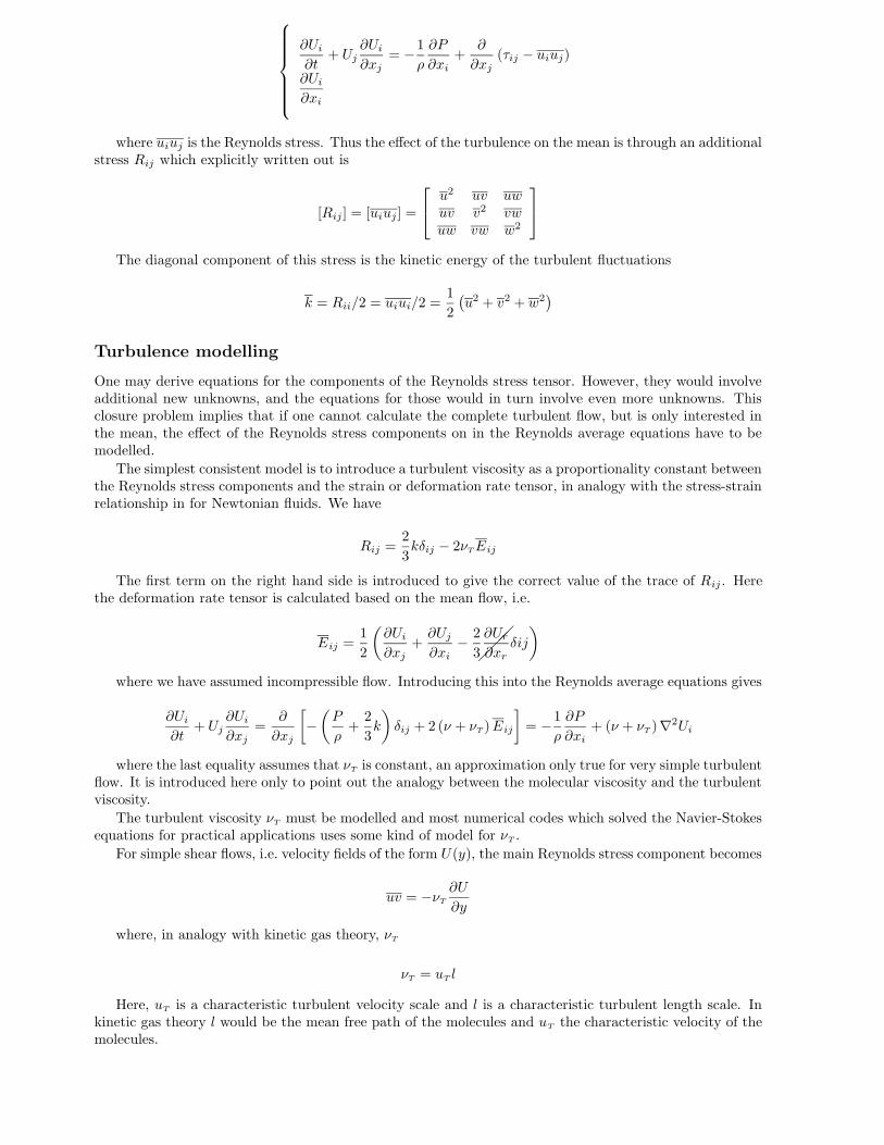
2.5. TURBULENT FLOW 55
∂Ui∂t
+ Uj∂Ui∂xj
= −1ρ
∂P
∂xi+
∂
∂xj(τij − uiuj)
∂Ui∂xi
where uiuj is the Reynolds stress. Thus the effect of the turbulence on the mean is through an additionalstress Rij which explicitly written out is
[Rij ] = [uiuj ] =
u2 uv uwuv v2 vwuw vw w2
The diagonal component of this stress is the kinetic energy of the turbulent fluctuations
k = Rii/2 = uiui/2 =1
2
(u2 + v2 + w2
)
Turbulence modelling
One may derive equations for the components of the Reynolds stress tensor. However, they would involveadditional new unknowns, and the equations for those would in turn involve even more unknowns. Thisclosure problem implies that if one cannot calculate the complete turbulent flow, but is only interested inthe mean, the effect of the Reynolds stress components on in the Reynolds average equations have to bemodelled.
The simplest consistent model is to introduce a turbulent viscosity as a proportionality constant betweenthe Reynolds stress components and the strain or deformation rate tensor, in analogy with the stress-strainrelationship in for Newtonian fluids. We have
Rij =2
3kδij − 2νTEij
The first term on the right hand side is introduced to give the correct value of the trace of Rij . Herethe deformation rate tensor is calculated based on the mean flow, i.e.
Eij =1
2
(∂Ui∂xj
+∂Uj∂xi
− 23¡¡¡
∂Ur∂xr
δij
)
where we have assumed incompressible flow. Introducing this into the Reynolds average equations gives
∂Ui∂t
+ Uj∂Ui∂xj
=∂
∂xj
[
−(P
ρ+2
3k
)
δij + 2 (ν + νT )Eij
]
= −1ρ
∂P
∂xi+ (ν + νT )∇2Ui
where the last equality assumes that νT is constant, an approximation only true for very simple turbulentflow. It is introduced here only to point out the analogy between the molecular viscosity and the turbulentviscosity.
The turbulent viscosity νT must be modelled and most numerical codes which solved the Navier-Stokesequations for practical applications uses some kind of model for νT .
For simple shear flows, i.e. velocity fields of the form U(y), the main Reynolds stress component becomes
uv = −νT
∂U
∂y
where, in analogy with kinetic gas theory, νT
νT = uT l
Here, uT is a characteristic turbulent velocity scale and l is a characteristic turbulent length scale. Inkinetic gas theory l would be the mean free path of the molecules and uT the characteristic velocity of themolecules.

56 CHAPTER 2. FLOW PHYSICS
!"!"!"!"!"!"!"!"!"!"!"!"!"!#"#"#"#"#"#"#"#"#"#"#"#"#"#
PSfrag replacements
x, x1y, x2z, x3u, u1v, u2w, u3x1x2x 0i
ri(x 0i , t
)
ui(x 0i , t
)
P(t = 0
)
xu1
u2 > u1x1x2x3x 0i
ui dtdx 0
i
dui dtri(dt)
dri(dt)
P1
P2
x1x2x3R3
R2
R1
r3
r2
r1π2 + dϕ12
V (t)S (t)
V (t+∆t)− V (t)S (t+∆t)
un
V (t+∆t)
pT0, U0
TwLT0U0
Gradient fieldswi∂p∂xi
uiDivergence free vectorfields // to boundary
Lhx1x2
p0 > p1p1undS
u · n∆txyu0p0
η = y√4νtuu0
y = η√4νt
tηy
ωz =ω(η)·u0√
πνt
tLδ
ω ≈ 0U →y, vx, u
LUδu0
η = y√νx/u0
f ′ = uu0
Blasius profile
δ∗
xSeparation point
⇐= Pressure force
x
y
l
uT
Figure 2.31: Prantdl’s mixing length l is the length for which a fluid particle displaced in the normaldirection can be expected to retain its horizontal momentum.
Zero-equation models
The simplest model for uT and l is to model them algebraically.In simple free shear flows like jets, wakes and shear layers we can take νT as constant in normal direction
or y-direction and to vary in a self-similar manner in x.In wall bounded shear flow we can take l as Prandtl’s mixing length (1920’s). This is a normal distance
over which the particle retains its momentum and is depicted in figure 2.31.We can thus evaluate uT and find νT
uT = l
∣∣∣∣
dU
dy
∣∣∣∣
⇒ νT = l2∣∣∣∣
dU
dy
∣∣∣∣
Define τw as the shear stress at the wall and uτ =√
τw/ρ as the skin friction velocity. With
uT = uτ , l = κ · yas Prandtl’s estimation of mixing length we get
dU
dy=uT
l=uτκy
⇒ U
uτ=1
κln y + C.
κ is the von Karman constant, approximately equal to 0.41. Thus the mixing length is proportional tothe distant from the wall and the region close to the wall in a turbulent flow has a logarithmic velocityprofile, called the log-region.
One-equation models
Instead of modelling the characteristic turbulent velocity algebraically, the next level of modelling uses theassumption that
uT =√
k =
√
1
2uiui
and a differential equation is used to calculate the turbulent kinetic energy. We can derive such anequation by taking the previously derived equation for Ui + ui and subtracting the equation for U , theReynolds average equation. We find
∂ui∂t
+ Uj∂ui∂xj
= −uj∂Ui∂xj
− uj∂ui∂xj
+∂
∂xj
(
−pρδij + ν
∂ui∂xj
+ uiuj
)
We now take the average of the inner product between the turbulent fluctuations ui and the aboveequation, and find
∂
∂t
(1
2uiui
)
+ Uj∂
∂xj
(1
2uiui
)
= −uiuj∂Ui∂xj
+∂
∂xj
(
−pujρ− 12uiuiuj +
ν
2
∂
∂xjuiui
)
− ν ∂ui∂xj
∂ui∂xj
︸ ︷︷ ︸
ε
where ε is the mean dissipation rate of the turbulent kinetic energy. We have now introduced a numberof new unknowns which have to be modelled.

2.5. TURBULENT FLOW 57
First, we model the Reynolds stress as previously indicated, i.e. uiuj =23kδij − νT
(∂Ui
∂xj+
∂Uj
∂xi
)
.
Second, the turbulent dissipation is modelled purely based on dimension using k and l. We have
ε = cD
k3/2
l
since the dimension of ε is [ε] = L2
T . Here cD is a modelling constant.Third, a gradient diffusion model is used for the transport terms, i.e.
−12uiuiuj −
1
ρpuj =
νT
Prk
∂k
∂xj
where Prk is the turbulent Prandtl number.For simplicity we write the resulting equation for the turbulent kinetic energy for constant νT . We find
Dk
Dt= (ν + νT )∇2k − uiuj
∂Ui
∂xj− ε
rate of increase diffusion rate generation rate dissipation rate
Two-equation models
The most popular model in use in engineering applications is a two equation model, the so called k-ε-model.This is based on the above model for k but instead of modelling ε a partial differential equation is derivedgoverning the turbulent dissipation. This equation has the form as the equation for k, with a diffusionterm, a generation term and a dissipation term. Many new model constants need to be introduced in orderto close the ε equation.
Once k and ε is calculated the turbulent viscosity is evaluated as a quotient of the two, such that thedimension is correct. We have
⇒ νT = Cµ ·k2
ε
where Cµ is a modelling constant.

58 CHAPTER 2. FLOW PHYSICS

Chapter 3
Finite volume methods for
incompressible flow
3.1 Finite Volume method on arbitrary grids
Equations with 1st order derivatives: the continuity equation
In finite volume methods one makes approximations of the differential equations in integral form. We startwith an equation with only first order derivatives, the continuity equation. Recall that the integral from ofthis equation can be written
∫
V
∂
∂xk(uk) dV =
∫
S
uknk dS = 0
Evaluating the normal vector ni to the curve l for two-dimensional flow, see figure 3.1, we have thenormal with length dl as ndl = (dy,−dx). This implies that
∫
S
uknk dl =
∫
S
(udy − v dx) = 0
We now apply this to an arbitrary two-dimensional grid defined as in figure 3.2.
We make use of the following definitions and approximations
uab = ui+ 12 ,j ≈ (ui+1,j + ui,j) /2 ∆xab = xb − xa
vab = vi+ 12 ,j ≈ (vi+1,j + vi,j) /2 ∆yab = yb − ya
PSfrag replacements
x, x1y, x2z, x3u, u1v, u2w, u3x1x2x 0i
ri(x 0i , t
)
ui(x 0i , t
)
P(t = 0
)
xu1
u2 > u1x1x2x3x 0i
ui dtdx 0
i
dui dtri(dt)
dri(dt)
P1
P2
x1x2x3R3
R2
R1
r3
r2
r1π2 + dϕ12
V (t)S (t)
V (t+∆t)− V (t)S (t+∆t)
un
V (t+∆t)
pT0, U0
TwLT0U0
Gradient fieldswi∂p∂xi
uiDivergence free vectorfields // to boundary
Lhx1x2
p0 > p1p1undS
u · n∆txyu0p0
η = y√4νtuu0
y = η√4νt
tηy
ωz =ω(η)·u0√
πνt
tLδ
ω ≈ 0U →y, vx, u
LUδu0
η = y√νx/u0
f ′ = uu0
Blasius profile
δ∗
xSeparation point
⇐= Pressure forcexy
luT
x
y
dx
dy
dy
−dx
dl = (dx, dy)
ndl = (dy,−dx)
Figure 3.1: Normal vector to the curve l.
59

60 CHAPTER 3. FINITE VOLUME METHODS FOR INCOMPRESSIBLE FLOW
$%$%$%$%$%$%$%$%$$%$%$%$%$%$%$%$%$$%$%$%$%$%$%$%$%$$%$%$%$%$%$%$%$%$$%$%$%$%$%$%$%$%$$%$%$%$%$%$%$%$%$$%$%$%$%$%$%$%$%$$%$%$%$%$%$%$%$%$$%$%$%$%$%$%$%$%$
&%&%&%&%&%&%&%&%&&%&%&%&%&%&%&%&%&&%&%&%&%&%&%&%&%&&%&%&%&%&%&%&%&%&&%&%&%&%&%&%&%&%&&%&%&%&%&%&%&%&%&&%&%&%&%&%&%&%&%&&%&%&%&%&%&%&%&%&&%&%&%&%&%&%&%&%&
PSfrag replacements
x, x1y, x2z, x3u, u1v, u2w, u3x1x2x 0i
ri(x 0i , t
)
ui(x 0i , t
)
P(t = 0
)
xu1
u2 > u1x1x2x3x 0i
ui dtdx 0
i
dui dtri(dt)
dri(dt)
P1
P2
x1x2x3R3
R2
R1
r3
r2
r1π2 + dϕ12
V (t)S (t)
V (t+∆t)− V (t)S (t+∆t)
un
V (t+∆t)
pT0, U0
TwLT0U0
Gradient fieldswi∂p∂xi
uiDivergence free vectorfields // to boundary
Lhx1x2
p0 > p1p1undS
u · n∆txyu0p0
η = y√4νtuu0
y = η√4νt
tηy
ωz =ω(η)·u0√
πνt
tLδ
ω ≈ 0U →y, vx, u
LUδu0
η = y√νx/u0
f ′ = uu0
Blasius profile
δ∗
xSeparation point
⇐= Pressure forcexy
luT
xy
dxdy
−dxdl = (dx, dy)
ndl = (dy,−dx)
i− 1, j + 1 i, j + 1 i+ 1, j + 1
c c′ b b′
i− 1, j i+ 1, j
i, j
Aabcd
d d′ a a′
i− 1, j − 1i, j − 1 i+ 1, j − 1
Figure 3.2: Arbitrary grid. Note that the grid lines need not be parallel to the coordinate directions.
with analogous expressions for the quantities on the bc, cd and da faces. We can now evaluate theintegral associated with the two-dimensional version of the continuity equation for the surface defined bythe points abcd. We have
∫
S
(udy − v dx) ≈ ui+ 12 ,j∆yab − vi+ 12 ,j∆xab + ui,j+ 12∆ybc − vi,j+ 12∆xbc +
ui− 12 ,j∆ycd − vi− 12 ,j∆xcd + ui,j− 12∆yda − vi,j− 12∆xda
On a cartesian grid we have the relations
∆xab = ∆xcd = ∆ybc = ∆yda = 0 and ∆ycd = −∆yab,∆xbc = −∆xdawhich implies that the approximation of the continuity equation can be written
∫
S
(udy − v dx) ≈(
ui+ 12 ,j − ui− 12 ,j)
∆yab +(
vi,j+ 12 + vi,j− 12
)
∆xda =
1
2(ui+1,j − ui−1,j)∆yab +
1
2(vi,j+1 − vi,j−1)∆xda
Note that dividing with ∆yab ·∆xda gives a standard central difference discretization of the continuityequation, i.e.
ui+1,j − ui−1,j2∆xda
+vi,j+1 − vi,j−1
2∆yab= 0
Equations with 2nd derivatives: the Laplace equation
We use the Gauss or Greens theorem to derive the integral from of the two-dimensional Laplace equation.We find
0 =
∫
V
∂2Φ
∂xj∂xjdV =
∫
S
∂φ
∂xjnj dS = 2D =
∫
S
(∂Φ
∂xdy − ∂Φ
∂ydx
)
If we approximate this integral in the same manner as for the continuity equation we have
[∂Φ
∂x
]
i+ 12 ,j
∆yab −[∂Φ
∂y
]
i+ 12 ,j
∆xab +
[∂Φ
∂x
]
i,j+ 12
∆ybc −[∂Φ
∂y
]
i,j+ 12
∆xbc +
[∂Φ
∂x
]
i− 12 ,j∆ycd −
[∂Φ
∂y
]
i− 12 ,j∆xcd +
[∂Φ
∂x
]
i,j− 12∆yda −
[∂Φ
∂y
]
i,j− 12∆xda

3.1. FINITE VOLUME METHOD ON ARBITRARY GRIDS 61
First derivatives are evaluated as mean value over adjacent control volumes (areas in the two-dimensionalcase). We use Gauss theorem over the area defined by the points a′b′c′d′, see figure 3.2. For the three-dimensional case we have
1
V
∫
V
∂Φ
∂xjdV =
1
V
∫
S
Φnj dS ⇒
which in the two-dimensional case is approximated by
([∂Φ
∂x
]
i+ 12 ,j
,
[∂Φ
∂y
]
i+ 12 ,j
)
≈ 1
Aa′b′c′d′
∫
a′b′c′d′
(Φdy,−Φdx)
where
∫
a′b′c′d′
Φdy ≈ Φi+1,j∆ya′b′ +Φb∆yb′c′ +Φi,j∆yc′d′ +Φ∆yd′a′
and the area evaluated as half magnitude of cross products of diagonals, i.e.
Aab ≡ Aa′b′c′d′ =1
2
∣∣∣∆xd′b′ ·∆ya′c′ −∆yd′b′ ·∆xa′c′
∣∣∣
and the value Φa is taken as the average
Φa =1
4(Φi,j +Φi+1,j +Φi,j−1 +Φi+1,j−1)
Evaluating the derivatives ∂Φ∂x ,
∂Φ∂y along the other cell faces and substituting back we obtain a 9 point
formula which couples all of the nine points around the point i, j, of the form
Ai,jΦi+1,j+1 + Bi,jΦi+1,j + Ci,jΦi+1,j−1 + Di,jΦi,j+1 + Ei,jΦi,j +Fi,jΦi,j−1 + Gi,jΦi−1,j+1 + Hi,jΦi−1,j + Ii,jΦi−1,j−1 = 0
If we have a total of N = m × n interior nodes, we obtain N equations which in matrix form can bewritten
Ax = b
Here xT = (Φ11,Φ12,Φ13, . . . ,Φmn) and b contains the boundary conditions. The matrix A is a N ×Nwith the terms Aij , Bij , etc. as coefficients.
Rather than showing the general case in more detail, we instead work out the expression for cartesiangrids in two-dimensions. We find
∫ (∂2Φ
∂x2+∂2Φ
∂y2
)
dxdy =
∫ (∂Φ
∂xdy − ∂Φ
∂ydx
)
≈([
∂Φ
∂x
]
i+ 12 ,j+
−[∂Φ
∂x
]
i− 12 ,j
)
∆y +
([∂Φ
∂y
]
i,j+ 12
−[∂Φ
∂y
]
i,j− 12
)
∆x
We can evaluate the derivatives as
[∂Φ
∂x
]
i+ 12 ,j
= (Φi+1,j − Φi,j)∆y ·1
∆x ·∆y
and so on for the rest of the terms, which implies that
∫ (∂Φ
∂xdy − ∂Φ
∂ydx
)
≈ (Φi+1,j − 2Φi,j +Φi−1,j)∆y
∆x+ (Φi,j+1 − 2Φi,j +Φi,j−1)
∆x
∆y
Dividing with the area ∆x ·∆y we obtain the usual 5-point Laplace formula, i. e.
Φi+1,j − 2φi,j +Φi−1,j∆x2
+Φi,j+1 − 2φi,j +Φi,j−1
∆y2= 0
which of course also can be written in the matrix form shown for the general case above.
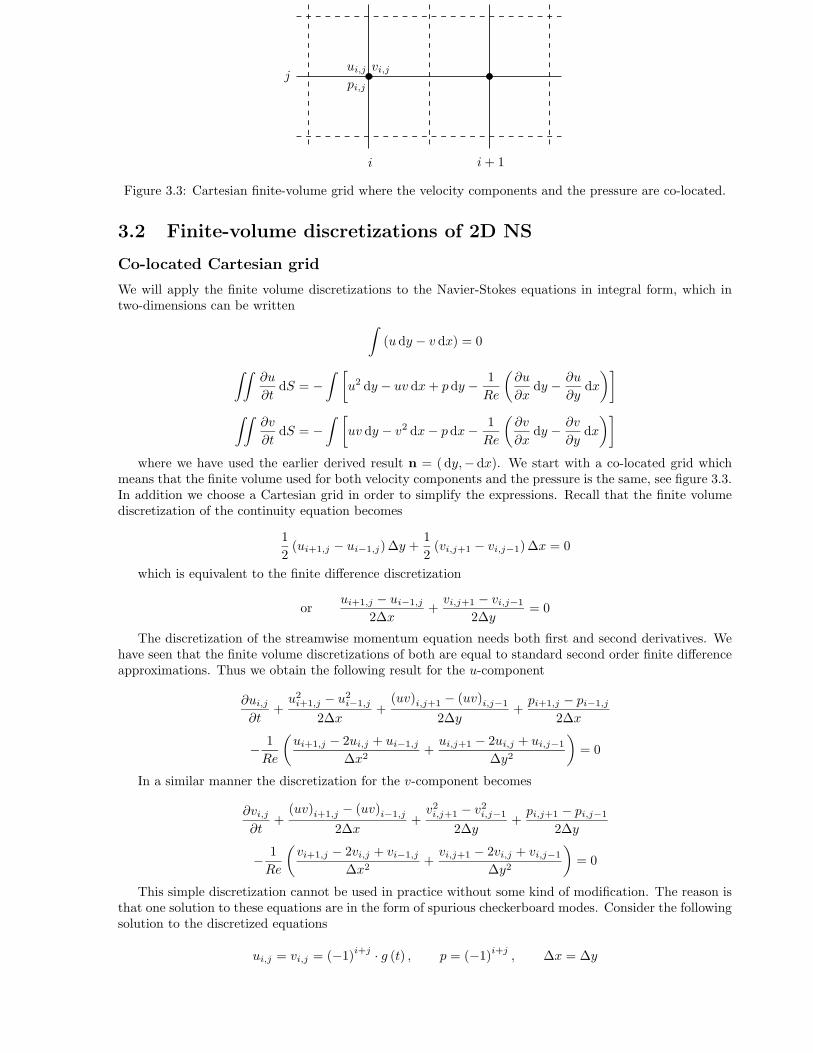
62 CHAPTER 3. FINITE VOLUME METHODS FOR INCOMPRESSIBLE FLOW
PSfrag replacements
x, x1y, x2z, x3u, u1v, u2w, u3x1x2x 0i
ri(x 0i , t
)
ui(x 0i , t
)
P(t = 0
)
xu1
u2 > u1x1x2x3x 0i
ui dtdx 0
i
dui dtri(dt)
dri(dt)
P1
P2
x1x2x3R3
R2
R1
r3
r2
r1π2 + dϕ12
V (t)S (t)
V (t+∆t)− V (t)S (t+∆t)
un
V (t+∆t)
pT0, U0
TwLT0U0
Gradient fieldswi∂p∂xi
uiDivergence free vectorfields // to boundary
Lhx1x2
p0 > p1p1undS
u · n∆txyu0p0
η = y√4νtuu0
y = η√4νt
tηy
ωz =ω(η)·u0√
πνt
tLδ
ω ≈ 0U →y, vx, u
LUδu0
η = y√νx/u0
f ′ = uu0
Blasius profile
δ∗
xSeparation point
⇐= Pressure forcexy
luT
xy
dxdy
−dxdl = (dx, dy)
ndl = (dy,−dx)i− 1, j + 1
i, j + 1i+ 1, j + 1
cc′
bb′
i− 1, ji+ 1, j
i, jAabcd
dd′
aa′
i− 1, j − 1i, j − 1
i+ 1, j − 1j
i i+ 1
ui,j vi,jpi,j
Figure 3.3: Cartesian finite-volume grid where the velocity components and the pressure are co-located.
3.2 Finite-volume discretizations of 2D NS
Co-located Cartesian grid
We will apply the finite volume discretizations to the Navier-Stokes equations in integral form, which intwo-dimensions can be written
∫
(udy − v dx) = 0
∫∫∂u
∂tdS = −
∫ [
u2 dy − uv dx+ pdy − 1
Re
(∂u
∂xdy − ∂u
∂ydx
)]
∫∫∂v
∂tdS = −
∫ [
uv dy − v2 dx− pdx− 1
Re
(∂v
∂xdy − ∂v
∂ydx
)]
where we have used the earlier derived result n = (dy,−dx). We start with a co-located grid whichmeans that the finite volume used for both velocity components and the pressure is the same, see figure 3.3.In addition we choose a Cartesian grid in order to simplify the expressions. Recall that the finite volumediscretization of the continuity equation becomes
1
2(ui+1,j − ui−1,j)∆y +
1
2(vi,j+1 − vi,j−1)∆x = 0
which is equivalent to the finite difference discretization
orui+1,j − ui−1,j
2∆x+vi,j+1 − vi,j−1
2∆y= 0
The discretization of the streamwise momentum equation needs both first and second derivatives. Wehave seen that the finite volume discretizations of both are equal to standard second order finite differenceapproximations. Thus we obtain the following result for the u-component
∂ui,j∂t
+u2i+1,j − u2i−1,j
2∆x+(uv)i,j+1 − (uv)i,j−1
2∆y+pi+1,j − pi−1,j
2∆x
− 1
Re
(ui+1,j − 2ui,j + ui−1,j
∆x2+ui,j+1 − 2ui,j + ui,j−1
∆y2
)
= 0
In a similar manner the discretization for the v-component becomes
∂vi,j∂t
+(uv)i+1,j − (uv)i−1,j
2∆x+v2i,j+1 − v2i,j−1
2∆y+pi,j+1 − pi,j−1
2∆y
− 1
Re
(vi+1,j − 2vi,j + vi−1,j
∆x2+vi,j+1 − 2vi,j + vi,j−1
∆y2
)
= 0
This simple discretization cannot be used in practice without some kind of modification. The reason isthat one solution to these equations are in the form of spurious checkerboard modes. Consider the followingsolution to the discretized equations
ui,j = vi,j = (−1)i+j · g (t) , p = (−1)i+j , ∆x = ∆y
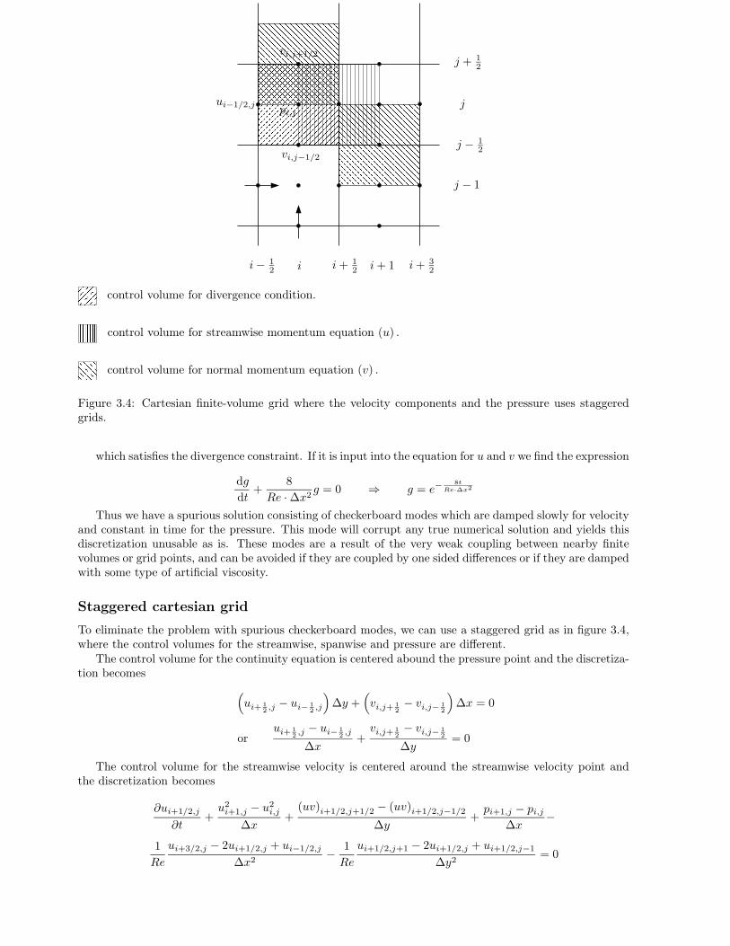
3.2. FINITE-VOLUME DISCRETIZATIONS OF 2D NS 63
'('('('('('('('(''('('('('('('('(''('('('('('('('(''('('('('('('('(''('('('('('('('(''('('('('('('('(''('('('('('('('(''('('('('('('('('
)()()()()()()())()()()()()()())()()()()()()())()()()()()()())()()()()()()())()()()()()()())()()()()()()())()()()()()()()*(*(*(*(*(*(*(**(*(*(*(*(*(*(**(*(*(*(*(*(*(**(*(*(*(*(*(*(*+(+(+(+(+(+(+(++(+(+(+(+(+(+(++(+(+(+(+(+(+(++(+(+(+(+(+(+(+,(,(,(,(,(,(,(,,(,(,(,(,(,(,(,,(,(,(,(,(,(,(,,(,(,(,(,(,(,(,-(-(-(-(-(-(-(--(-(-(-(-(-(-(--(-(-(-(-(-(-(--(-(-(-(-(-(-(-
.(.(.(.(.(.(.(..(.(.(.(.(.(.(..(.(.(.(.(.(.(..(.(.(.(.(.(.(./(/(/(/(/(/(/(//(/(/(/(/(/(/(//(/(/(/(/(/(/(//(/(/(/(/(/(/(/
PSfrag replacements
x, x1y, x2z, x3u, u1v, u2w, u3x1x2x 0i
ri(x 0i , t
)
ui(x 0i , t
)
P(t = 0
)
xu1
u2 > u1x1x2x3x 0i
ui dtdx 0
i
dui dtri(dt)
dri(dt)
P1
P2
x1x2x3R3
R2
R1
r3
r2
r1π2 + dϕ12
V (t)S (t)
V (t+∆t)− V (t)S (t+∆t)
un
V (t+∆t)
pT0, U0
TwLT0U0
Gradient fieldswi∂p∂xi
uiDivergence free vectorfields // to boundary
Lhx1x2
p0 > p1p1undS
u · n∆txyu0p0
η = y√4νtuu0
y = η√4νt
tηy
ωz =ω(η)·u0√
πνt
tLδ
ω ≈ 0U →y, vx, u
LUδu0
η = y√νx/u0
f ′ = uu0
Blasius profile
δ∗
xSeparation point
⇐= Pressure forcexy
luT
xy
dxdy
−dxdl = (dx, dy)
ndl = (dy,−dx)i− 1, j + 1
i, j + 1i+ 1, j + 1
cc′
bb′
i− 1, ji+ 1, j
i, jAabcd
dd′
aa′
i− 1, j − 1i, j − 1
i+ 1, j − 1j
ii+ 1ui,jvi,jpi,j
pi,j
vi,j+1/2
vi,j−1/2
ui−1/2,j
i− 12 i i+ 1
2 i+ 1 i+ 32
j + 12
j
j − 12
j − 1
00001111
PSfrag replacements
x, x1y, x2z, x3u, u1v, u2w, u3x1x2x 0i
ri(x 0i , t
)
ui(x 0i , t
)
P(t = 0
)
xu1
u2 > u1x1x2x3x 0i
ui dtdx 0
i
dui dtri(dt)
dri(dt)
P1
P2
x1x2x3R3
R2
R1
r3
r2
r1π2 + dϕ12
V (t)S (t)
V (t+∆t)− V (t)S (t+∆t)
un
V (t+∆t)
pT0, U0
TwLT0U0
Gradient fieldswi∂p∂xi
uiDivergence free vectorfields // to boundary
Lhx1x2
p0 > p1p1undS
u · n∆txyu0p0
η = y√4νtuu0
y = η√4νt
tηy
ωz =ω(η)·u0√
πνt
tLδ
ω ≈ 0U →y, vx, u
LUδu0
η = y√νx/u0
f ′ = uu0
Blasius profile
δ∗
xSeparation point
⇐= Pressure forcexy
luT
xy
dxdy
−dxdl = (dx, dy)
ndl = (dy,−dx)i− 1, j + 1
i, j + 1i+ 1, j + 1
cc′
bb′
i− 1, ji+ 1, j
i, jAabcd
dd′
aa′
i− 1, j − 1i, j − 1
i+ 1, j − 1j
ii+ 1ui,jvi,jpi,jpi,j
vi,j+1/2vi,j−1/2ui−1/2,ji− 1
2
ii+ 1
2
i+ 1i+ 3
2j + 1
2
jj − 1
2
j − 1control volume for divergence condition.
2323232232323243434344343434
PSfrag replacements
x, x1y, x2z, x3u, u1v, u2w, u3x1x2x 0i
ri(x 0i , t
)
ui(x 0i , t
)
P(t = 0
)
xu1
u2 > u1x1x2x3x 0i
ui dtdx 0
i
dui dtri(dt)
dri(dt)
P1
P2
x1x2x3R3
R2
R1
r3
r2
r1π2 + dϕ12
V (t)S (t)
V (t+∆t)− V (t)S (t+∆t)
un
V (t+∆t)
pT0, U0
TwLT0U0
Gradient fieldswi∂p∂xi
uiDivergence free vectorfields // to boundary
Lhx1x2
p0 > p1p1undS
u · n∆txyu0p0
η = y√4νtuu0
y = η√4νt
tηy
ωz =ω(η)·u0√
πνt
tLδ
ω ≈ 0U →y, vx, u
LUδu0
η = y√νx/u0
f ′ = uu0
Blasius profile
δ∗
xSeparation point
⇐= Pressure forcexy
luT
xy
dxdy
−dxdl = (dx, dy)
ndl = (dy,−dx)i− 1, j + 1
i, j + 1i+ 1, j + 1
cc′
bb′
i− 1, ji+ 1, j
i, jAabcd
dd′
aa′
i− 1, j − 1i, j − 1
i+ 1, j − 1j
ii+ 1ui,jvi,jpi,jpi,j
vi,j+1/2vi,j−1/2ui−1/2,ji− 1
2
ii+ 1
2
i+ 1i+ 3
2j + 1
2
jj − 1
2
j − 1control volume for divergence condition.
control volume for streamwise momentum equation (u) .
55556666
PSfrag replacements
x, x1y, x2z, x3u, u1v, u2w, u3x1x2x 0i
ri(x 0i , t
)
ui(x 0i , t
)
P(t = 0
)
xu1
u2 > u1x1x2x3x 0i
ui dtdx 0
i
dui dtri(dt)
dri(dt)
P1
P2
x1x2x3R3
R2
R1
r3
r2
r1π2 + dϕ12
V (t)S (t)
V (t+∆t)− V (t)S (t+∆t)
un
V (t+∆t)
pT0, U0
TwLT0U0
Gradient fieldswi∂p∂xi
uiDivergence free vectorfields // to boundary
Lhx1x2
p0 > p1p1undS
u · n∆txyu0p0
η = y√4νtuu0
y = η√4νt
tηy
ωz =ω(η)·u0√
πνt
tLδ
ω ≈ 0U →y, vx, u
LUδu0
η = y√νx/u0
f ′ = uu0
Blasius profile
δ∗
xSeparation point
⇐= Pressure forcexy
luT
xy
dxdy
−dxdl = (dx, dy)
ndl = (dy,−dx)i− 1, j + 1
i, j + 1i+ 1, j + 1
cc′
bb′
i− 1, ji+ 1, j
i, jAabcd
dd′
aa′
i− 1, j − 1i, j − 1
i+ 1, j − 1j
ii+ 1ui,jvi,jpi,jpi,j
vi,j+1/2vi,j−1/2ui−1/2,ji− 1
2
ii+ 1
2
i+ 1i+ 3
2j + 1
2
jj − 1
2
j − 1control volume for divergence condition.
control volume for streamwise momentum equation (u) .control volume for normal momentum equation (v) .
Figure 3.4: Cartesian finite-volume grid where the velocity components and the pressure uses staggeredgrids.
which satisfies the divergence constraint. If it is input into the equation for u and v we find the expression
dg
dt+
8
Re ·∆x2 g = 0 ⇒ g = e−8t
Re·∆x2
Thus we have a spurious solution consisting of checkerboard modes which are damped slowly for velocityand constant in time for the pressure. This mode will corrupt any true numerical solution and yields thisdiscretization unusable as is. These modes are a result of the very weak coupling between nearby finitevolumes or grid points, and can be avoided if they are coupled by one sided differences or if they are dampedwith some type of artificial viscosity.
Staggered cartesian grid
To eliminate the problem with spurious checkerboard modes, we can use a staggered grid as in figure 3.4,where the control volumes for the streamwise, spanwise and pressure are different.
The control volume for the continuity equation is centered abound the pressure point and the discretiza-tion becomes
(
ui+ 12 ,j − ui− 12 ,j)
∆y +(
vi,j+ 12 − vi,j− 12)
∆x = 0
orui+ 12 ,j − ui− 12 ,j
∆x+vi,j+ 12 − vi,j− 12
∆y= 0
The control volume for the streamwise velocity is centered around the streamwise velocity point andthe discretization becomes
∂ui+1/2,j
∂t+u2i+1,j − u2i,j
∆x+(uv)i+1/2,j+1/2 − (uv)i+1/2,j−1/2
∆y+pi+1,j − pi,j
∆x−
1
Re
ui+3/2,j − 2ui+1/2,j + ui−1/2,j∆x2
− 1
Re
ui+1/2,j+1 − 2ui+1/2,j + ui+1/2,j−1∆y2
= 0
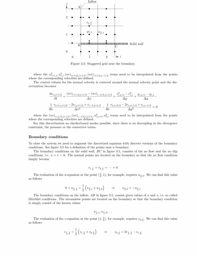
64 CHAPTER 3. FINITE VOLUME METHODS FOR INCOMPRESSIBLE FLOW
777777777777777777777777777777777777777777888888888888888888888888888888888888888888
PSfrag replacements
x, x1y, x2z, x3u, u1v, u2w, u3x1x2x 0i
ri(x 0i , t
)
ui(x 0i , t
)
P(t = 0
)
xu1
u2 > u1x1x2x3x 0i
ui dtdx 0
i
dui dtri(dt)
dri(dt)
P1
P2
x1x2x3R3
R2
R1
r3
r2
r1π2 + dϕ12
V (t)S (t)
V (t+∆t)− V (t)S (t+∆t)
un
V (t+∆t)
pT0, U0
TwLT0U0
Gradient fieldswi∂p∂xi
uiDivergence free vectorfields // to boundary
Lhx1x2
p0 > p1p1undS
u · n∆txyu0p0
η = y√4νtuu0
y = η√4νt
tηy
ωz =ω(η)·u0√
πνt
tLδ
ω ≈ 0U →y, vx, u
LUδu0
η = y√νx/u0
f ′ = uu0
Blasius profile
δ∗
xSeparation point
⇐= Pressure forcexy
luT
xy
dxdy
−dxdl = (dx, dy)
ndl = (dy,−dx)i− 1, j + 1
i, j + 1i+ 1, j + 1
cc′
bb′
i− 1, ji+ 1, j
i, jAabcd
dd′
aa′
i− 1, j − 1i, j − 1
i+ 1, j − 1j
ii+ 1ui,jvi,jpi,jpi,j
vi,j+1/2vi,j−1/2ui−1/2,ji− 1
2
ii+ 1
2
i+ 1i+ 3
2j + 1
2
jj − 1
2
j − 1 A
B C
u 32 ,1
v1, 32
p1,1
0
0
1
1
2
2
i
jInflow
Solid wall
Figure 3.5: Staggered grid near the boundary.
where the u2i+1,j , u2i,j , (uv)i+1/2,j+1/2 , (uv)i+1/2,j−1/2 terms need to be interpolated from the points
where the corresponding velocities are defined.
The control volume for the normal velocity is centered around the normal velocity point and the dis-cretization becomes
∂vi,j+1/2
∂t+(uv)i+1/2,j+1/2 − (uv)i−1/2,j+1/2
∆x+v2i,j+1 − v2i,j
∆y+pi,j+1 − pi,j
∆y−
1
Re
vi+1,j+1/2 − 2vi,j+1/2 + vi−1,j+1/2∆x2
− 1
Re
vi,j+3/2 − 2vi,j+1/2 + vi,j−1/2∆y2
= 0
where the (uv)i+1/2,j+1/2 , (uv)i−1/2,j+1/2 , u2i,j+1, u
2i,j terms need to be interpolated from the points
where the corresponding velocities are defined.
For this discretization no checkerboard modes possible, since there is no decoupling in the divergenceconstraint, the pressure or the convective terms.
Boundary conditions
To close the system we need to augment the discretized equation with discrete versions of the boundaryconditions. See figure 3.5 for a definition of the points near a boundary.
The boundary conditions on the solid wall, BC in figure 3.5, consists of the no flow and the no slipconditions, i.e. u = v = 0. The normal points are located on the boundary so that the no flow conditionsimply become
v1, 12 = v2, 12 = · · · = 0
The evaluation of the u-equation at the point ( 32 , 1), for example, requires u 32 ,0. We can find this valueas follows
0 = u 32 ,12=1
2
(
u 32 ,1+ u 3
2 ,0
)
⇒ u 32 ,0= −u 3
2 ,1
The boundary conditions on the inflow, AB in figure 3.5, consist given values of u and v, i.e. so calledDirichlet conditions. The streamwise points are located on the boundary so that the boundary conditionis simply consist of the known values
u 12 ,1, u 1
2 ,2, . . .
The evaluation of the v-equation at the point (1, 32 ), for example, requires v0, 32 . We can find this valueas follows
v 12 ,32=1
2
(
v1, 32 + v0,32
)
⇒ v0, 32 = 2v12 ,32− v1, 32

3.3. SUMMARY OF THE EQUATIONS 65
If AB in figure 3.5 is an outflow boundary, the boundary conditions may consist of ∂u∂x =
∂v∂x = 0, i.e.
so called Neumann conditions. These conditions should be evaluated at i = 12 . For the streamwise and
normal velocity we find
u− 12 ,2 = u 32 ,2, v0, 32 = v1, 32
Note that no reference is made to the pressure points outside the domain, so that in this formulationno boundary conditions for p is needed so far. However, depending on the particular discretization of thetime derivative and other the details of the solution method one may need to augment the the above withboundary conditions for the pressure. If this is the case particular care has to be taken so that thoseconditions do not upset the divergence free condition.
3.3 Summary of the equations
The discretized equations derived for the staggered grid can be written in the following form
∂ui+ 12 ,j
∂t+Ai+ 12 ,j +
pi+1,j − pi,j∆x
= 0
∂vi,j+ 12∂t
+Bi,j+ 12 +pi,j+1 − pi,j
∆y= 0
Di,j = 0
where the expression for the Ai+ 12 ,j can be written
Ai+ 12 ,j =
=u2i+1,j − u2i,j
∆x+(uv)i+ 12 ,j+
12− (uv)i+ 12 ,j− 12∆y
− 1
Re
ui+ 32 ,j − 2ui+ 12 ,j + ui− 12 ,j∆x2
− 1
Re
ui+ 12 ,j+1 − 2ui+ 12 ,j + ui+ 12 ,j−1∆y2
= expand and interpolate using grid values
=
[1
2∆x(ui+ 32 ,j − ui− 12 ,j) +
1
4∆y(vi+1,j+ 12 − vi,j+ 12 − vi+1,j− 12 − vi,j− 12 ) +
2
Re
(1
∆x2+
1
∆y2
)]
ui+ 12 ,j
+
(1
4∆xui+ 32 ,j −
1
Re∆x2
)
ui+ 32 ,j +
(1
4∆xui− 12 ,j −
1
Re∆x2
)
ui− 12 ,j
+
(1
4∆y(vi+1,j+ 12 + vi,j+
12)− 1
Re∆y2
)
ui+ 12 ,j+1 +
(1
4∆y(vi+1,j− 12 + vi,j− 12 )−
1
Re∆y2
)
ui+ 12 ,j−1
= a(u, v)i+ 12 ,jui+12 ,j+∑
nb
a(u, v)nbunb
The last line summarizes the expressions, where the sum over nb indicates a sum over the nearby nodes.The expression for Bi,j+ 12
can in a similar way be written
Bi,j+ 12 =
=(uv)i+ 12 ,j+
12− (uv)i− 12 ,j+ 12∆x
+v2i,j+1 − v2i,j
∆y
− 1R
vi+1,j+ 12 − 2vi,j+ 12 + vi−1,j+ 12∆x2
− 1
R
vi,j+ 32 − 2vi,j+ 12 + vi,j− 12∆y2
= expand and interpolate using grid values
= b(u, v)i,j+ 12 vi,j+12+∑
nb
b(u, v)nbvnb

66 CHAPTER 3. FINITE VOLUME METHODS FOR INCOMPRESSIBLE FLOW
where the expressions for b(u, v)i,j+ 12 and b(u, v)nb are analogous to a(u, v)i+ 12 ,j and a(u, v)nb, andtherefore not explicitly written out. The expression originating from the continuity equation is
Di,j =ui+ 12 ,j − ui− 12 ,j
∆x+vi,j+ 12 − vi,j− 12
∆y
These equations, including the boundary conditions, can be assembled into matrix form. We have
d
dt
uv0
+
A(u, v) 0 Gx
0 B(u, v) Gy
Dx Dy 0
uvp
=
fufv0
Here we we have used the definitions
u - vector of unknown streamwise velocitiesv - vector of unknown normal velocitiesp - vector of pressure unknownsA(u, v) - non-linear algebraic operator from advective and viscous terms of u-eq.B(u, v) - non-linear algebraic operator from advective and viscous terms of v-eq.Gx - linear algebraic operator from stremwise pressure gradientGy - linear algebraic operator from normal pressure gradientDx - linear algebraic operator from x-part of divergence constraintDy - linear algebraic operator from y-part of divergence constraintf - vector of source terms from BC
With obvious changes in notation, we can write the system of equations in an even more compact formas
d
dt
(u0
)
+
(N (u) GD 0
)(up
)
=
(f0
)
If this is compared to the finite element discretization in the next chapter, it is seen that the form ofthe discretized matrix equations are the same.
3.4 Time dependent flows
The projection method
For time-dependent flow a common way to solve the discrete equations is the projection or pressure correc-tion method. Sometimes this method and its generalizations are also called splitting methods. We illustratethe method using the system written in the compact notation defined above.
We start to discretize the time derivative with a first order explicit method
un+1 − un∆t
+N (un)un +Gpn+1 = f (tn)
Dun+1 = 0
Then we make a prediction of the velocity field at the next time step u∗ not satisfying continuity, andthen a correction involving p such that Dun+1 = 0. We have
u∗ − un∆t
+N (un)un = f (tn)
un+1 − u∗∆t
+Gpn+1 = 0
Dun+1 = 0
Next, apply the divergence operator D to the correction step
DGpn+1 =1
∆tD u∗
Here DG represents divgrad = Laplacian, i.e. discrete version of pressure Poisson equation. Thevelocity at the next time level thus becomes
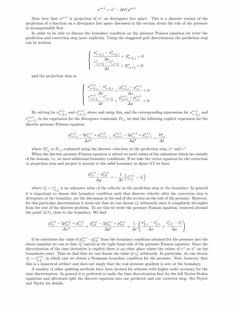
3.4. TIME DEPENDENT FLOWS 67
un+1 = u∗ −∆tG pn+1
Note here that un+1 is projection of u∗ on divergence free space. This is a discrete version of theprojection of a function on a divergence free space discussed in the section about the role of the pressurein incompressible flow.
In order to be able to discuss the boundary condition on the pressure Poisson equation we write theprediction and correction step more explicitly. Using the staggered grid discretization the prediction stepcan be written
u∗i+ 12 ,j
− uni+ 12 ,j
∆t+Ani+ 12 ,j
= 0
v∗i,j+ 12
− vni,j+ 12
∆t+Bn
i,j+ 12= 0
and the projection step as
un+1i+ 12 ,j
− u∗i+ 12 ,j
∆t+pn+1i+1,j − pn+1i,j
∆x= 0
vn+1i,j+ 12
− v∗i,j+ 12
∆t+pn+1i,j+1 − pn+1i,j
∆y= 0
By solving for un+1i+ 12 ,j
and vn+1i,j+ 12
above and using this, and the corresponding expressions for un+1i− 12 ,j
and
vn+1i,j− 12
, in the expression for the divergence constraint Di,j we find the following explicit expression for the
discrete pressure Poisson equation
pn+1i+1,j − 2pn+1i,j + pn+1i−1,j∆x2
+pn+1i,j+1 − 2pn+1i,j + pn+1i,j−1
∆y2=D∗i,j
∆t
where D∗i,j is Di,j evaluated using the discrete velocities at the prediction step, u
∗ and v∗.
When the discrete pressure Poisson equation is solved we need values of the unknowns which are outsideof the domain, i.e. we need additional boundary conditions. If we take the vector equation for the correctionor projection step and project it normal to the solid boundary in figure 3.5 we have
pn+12,1 − pn+12,0
∆y= − 1
∆t
(
vn+12, 12
− v∗Γ)
where v∗Γ = v∗2, 12
is an unknown value of the velocity in the prediction step at the boundary. In general
it is important to choose this boundary condition such that discrete velocity after the correction step isdivergence at the boundary, see the discussion in the end of the section on the role of the pressure. However,for this particular discretization it turns out that we can choose v∗Γ arbitrarily since it completely decouplesfrom the rest of the discrete problem. To see this we write the pressure Poisson equation, centered aboundthe point (2,1), close to the boundary. We find
pn+13,1 − 2pn+12,1 + pn+11,1
∆x2+pn+12,2 − 2pn+12,1 + pn+12,0
∆y2=
1
∆t
(u∗52 ,1− u∗3
2 ,1
∆x+v∗2, 32− v∗Γ∆y
)
if we substitute the value of pn+12,1 −pn+12,0 from the boundary condition obtained for the pressure into theabove equation we can se that v∗Γ cancels in the right hand side of the pressure Poisson equation. Since thediscretization of the time derivative is explicit there is no other place where the values of v∗ or u∗ on theboundaries enter. Thus we find that we can choose the value of v∗Γ arbitrarily. In particular, we can choosev∗Γ = vn+1
2, 12, in which case we obtain a Neumann boundary condition for the pressure. Note, however, that
this is a numerical artifact and does not imply that the real pressure gradient is zero at the boundary.
A number of other splitting methods have been devised for schemes with higher order accuracy for thetime discretization. In general it is preferred to make the time discretization first for the full Navier-Stokesequations and afterward split the discrete equation into one predictor and one corrector step. See Peyretand Taylor for details.

68 CHAPTER 3. FINITE VOLUME METHODS FOR INCOMPRESSIBLE FLOW
Time step restriction
For stability it is necessary that prediction step is stable, numerical evidence indicates that this is sufficient.In the predictor case the momentum equations decouple if we linearize them abound the solution U0, V0.It thus suffices to consider the equation
∂u
∂t+ U0
∂u
∂x+ V0
∂u
∂y=
1
Re∇2u
For simplicity we will here consider one-dimensional version
∂u
∂t+ U0
∂u
∂x=
1
Re
∂2u
∂x2
which in discretized form can be written
un+1j = unj +∆t
[
−U0unj+1 − unj−1
2∆x+1
Re
unj+1 − 2unj + unj−1∆x2
]
where we have chosen to call the discrete points where the u-velocity is evaluate for xj .We introduce
unj = Qn · ei·ωxj
into the discrete equation, together with the definitions
λ =U0∆t
∆x, α =
2∆t
Re∆x2, ξ = ω ·∆x
This implies that the amplification factor Q can be written
Q = 1− iλ sin (ξ)− 2α sin2(ξ
2
)
We find that the absolute value of Q satisfies
|Q| = 1− 4(λ2 − α2
)s2 + 4
(λ2 − s2
)s
= 1− 4s[(λ2 − α2
)s− λ2 + α
]≤ 1
where s = sin2(ξ2
)
. This implies that
Φ (s) = −(λ2 − α2
)s+ λ2 − α ≤ 0 ∀s : 0 ≤ s ≤ 1
Φ (s) is linear function of s and thus the the limiting condition on Φ (s) is given by its values at the twoend points of the s-interval. We find
Φ (0) = λ2 − α ≤ 0, Φ(1) = α2 − α ≤ 0which implies that
⇒ λ2 ≤ α ≤ 1substituting back the definitions of λ and α we find the following stability conditions
1
2U20∆tRe ≤ 1
2∆t
Re∆x2≤ 1
For the two dimensional version of the predictor step Peyret and Taylor [8] find the following stabilitylimits
1
4
(U20 + V
20
)∆t ·Re ≤ 1
4∆t
Re∆x2≤ 1
Note that this is a stronger condition than in the one-dimensional case.
3.5. GENERAL ITERATION METHODS FOR STEADY FLOWS 69
3.5 General iteration methods for steady flows
Distributive iteration
For steady flows we can still use the methods introduced for unsteady flows, and iterate the solution in timeto obtain a steady state. However, in many cases it is more effective to use other iteration methods. We willhere introduce a general distributive iteration method and apply it to the discretized steady Navier-Stokesequations.
For the steady case the discretized equations can be written in the form
(N(u) GD 0
)(up
)
=
(f0
)
which is of the form Ay = b. Now, let y = B y which implies that
AB y = b
and use the iteration scheme on this modified equation. We divide the matrix AB in the followingmanner
AB =M − T ⇒ M y = T y + b
and use this to define the iteration scheme
MB−1 yk+1 = TB−1 yk + b =MB−1 yk + b−Ayk
which can be simplified to
yk+1 = yk +BM−1 (b−Ayk)
︸ ︷︷ ︸
rk
where rk is the residual error in the k:th step of the iteration procedure.If B = I we obtain a regular iteration method where residual rk is used to update yk by inverting M ,
a simplified part of A, as in the Gauss-Seidell method for example. For this method we have
Ax = bA = L− U(L− U)x = bLxn+1 = U xn + b
Application to the steady Navier-Stokes equations
When the distributive iteration method is applied to the steady Naiver-Stokes we have
A =
(N(u) GD 0
)
we can obtain AB in the following block triangular form
AB =
(N(u) 0D −DN(u)−1G
)
if the matrix B has the form
B =
(I −N(u)−1G0 I
)
≈(
I −N(u)−1G0 I
)
where N(u)−1 is a simple approximation of the inverse of the discrete Navier-Stokes operator. We nowsplit AB =M − T where
M =
(Q 0D R
)
and where Q is an approximation of N(u) and R is an approximation of −DN−1G. Note that R is adiscrete Laplace like operator.

70 CHAPTER 3. FINITE VOLUME METHODS FOR INCOMPRESSIBLE FLOW
The SIMPLE (Semi-Implicit Method for Pressure Linked Equations) by Pantankar and Spalding (1972)can be thought of as a distributive iteration method. Wesseling [10] indicates that by choosing
N(u)−1 = [diagN(uk)]−1
Q = N(uk)
R = −D[diagN(uk)]−1G
we have a method which is essentially the original version of the SIMPLE method. Thus we have thefollowing iteration steps
1. First, we calculate the residual
b−Ayk =(f0
)
−(N(uk) GD 0
)(uk
pk
)
=
(rk1rk2
)
2. Second, we calculate M−1rk which implies
Qδu = rk1 ⇒ δu = Q−1 rk1
Rδp = rk2 −D δu
3. Third, we have the distribution step BM−1 rk which becomes
(δuδp
)
= B
(δuδp
)
=
(
δu− N−1Gδpδp
)
4. Fourth, there is an under relaxation step, where the velocities and the pressure is updated
uk+1 = uk + ωuδupk+1 = pk + ωpδp
The under relaxation is needed for the method to converge, thus ωu and ωp is usually substantiallylower that one.

Chapter 4
Finite element methods for
incompressible flow
The finite-element method (FEM) approximates an integral form of the governing equations. However,the integral form—called the variational form—is usually different from the one used for the finite-volumemethod. Moreover, different integral forms may be used for the same equation depending on circumstancessuch as boundary conditions. We introduce FEM first for a scalar advection–diffusion problem beforediscussing the Navier–Stokes equations.
4.1 FEM for an advection–diffusion problem
We consider the steady flow of an incompressible fluid in a bounded domain Ω, and we assume that itsvelocity field Uj is known (from a previous numerical solution, for instance). We assume that the boundaryΓ of the domain can be decomposed into two portions Γ0 and Γ1, as in figure 4.1 for instance. We areinterested to compute the temperature field u in the domain, modeled by the advection–diffusion problem
Uj∂u
∂xj− ν∇2u = f in Ω, (4.1a)
u = 0 on Γ0, (4.1b)
∂u
∂n= 0 on Γ1. (4.1c)
The coefficient ν > 0 is the thermal diffusivity. Incompressibility yields that∂Uj
∂xj= 0. We assume that
Γ1 is a solid wall, so that njUj = 0 on Γ1. This simplifies the analysis but is not essential. The Dirichletboundary condition u = 0 on Γ0 is called an isothermal condition, whereas the Neumann condition ∂u
∂n = 0on Γ1 is an adiabatic condition.
Deriving the integral form that is used to form the finite-element discretization requires some vectorcalculus. The product rule of differentiation yields
∂
∂xi
(
v∂u
∂xi
)
=∂v
∂xi
∂u
∂xi+ v∇2u. (4.2)
PSfrag replacements
x, x1y, x2z, x3u, u1v, u2w, u3x1x2x 0i
ri(x 0i , t
)
ui(x 0i , t
)
P(t = 0
)
xu1
u2 > u1x1x2x3x 0i
ui dtdx 0
i
dui dtri(dt)
dri(dt)
P1
P2
x1x2x3R3
R2
R1
r3
r2
r1π2 + dϕ12
V (t)S (t)
V (t+∆t)− V (t)S (t+∆t)
un
V (t+∆t)
pT0, U0
TwLT0U0
Gradient fieldswi∂p∂xi
uiDivergence free vectorfields // to boundary
Lhx1x2
p0 > p1p1undS
u · n∆txyu0p0
η = y√4νtuu0
y = η√4νt
tηy
ωz =ω(η)·u0√
πνt
tLδ
ω ≈ 0U →y, vx, u
LUδu0
η = y√νx/u0
f ′ = uu0
Blasius profile
δ∗
xSeparation point
⇐= Pressure forcexy
luT
xy
dxdy
−dxdl = (dx, dy)
ndl = (dy,−dx)i− 1, j + 1
i, j + 1i+ 1, j + 1
cc′
bb′
i− 1, ji+ 1, j
i, jAabcd
dd′
aa′
i− 1, j − 1i, j − 1
i+ 1, j − 1j
ii+ 1ui,jvi,jpi,jpi,j
vi,j+1/2vi,j−1/2ui−1/2,ji− 1
2
ii+ 1
2
i+ 1i+ 3
2j + 1
2
jj − 1
2
j − 1ABC
u 32 ,1
v1, 32p1,1
012ij
InflowSolid wall
n
Γ0
Γ1
Ω
Figure 4.1: A typical domain associated with the advection–diffusion problem (4.1).
71

72 CHAPTER 4. FINITE ELEMENT METHODS FOR INCOMPRESSIBLE FLOW
Recall the divergence theorem ∫
Ω
∂wi∂xi
dΩ =
∫
Γ
niwi dΓ. (4.3)
Integrating expression (4.2) and applying the divergence theorem on the left side yields
∫
Γ
v∂u
∂ndΓ =
∫
Ω
∂v
∂xi
∂u
∂xidΩ +
∫
Ω
v∇2udΩ. (4.4)
(Note that∂u
∂n= ni
∂u
∂xi.)
Let v be any smooth function such that v = 0 on Γ0. Multiplying equation (4.1a) with v, integratingover Ω, and utilizing expression (4.4) yields
∫
Ω
fv dΩ =
∫
Ω
vUj∂u
∂xjdΩ− ν
∫
Ω
v∇2udΩ =
∫
Ω
vUj∂u
∂xjdΩ + ν
∫
Ω
∂v
∂xj
∂u
∂xjdΩ− ν
¡¡¡¡µ0
∫
Γ
v∂u
∂ndΓ,
where the last term vanishes on Γ0 due to the requirements on v, and on Γ1 due to boundary condition (4.1c)We have thus shown that a smooth (twice continuously differentiable) solution to problem (4.1) (also
called a classical solution) satisfies the varational form
∫
Ω
vUj∂u
∂xjdΩ + ν
∫
Ω
∂v
∂xj
∂u
∂xjdΩ =
∫
Ω
fv dΩ (4.5)
for each smooth function v vanishing on Γ0We will now “forget” about the differential equation (4.1), and directly consider the variational form (4.5).
For this, we need to introduce the function space
V =
v :
∫
Ω
∂v
∂xi
∂v
∂xidΩ < +∞, v = 0 on Γ0
.
The space V is a linear space, that is, u, v ∈ V ⇒ αu + βv ∈ V ∀α, β ∈ R. The requirement that thegradient-square of each function in V is bounded should be intepreted as a requirement that the energy isbounded.
The variational problem will thus be
Find u ∈ V such that∫
Ω
vUj∂u
∂xjdΩ + ν
∫
Ω
∂v
∂xj
∂u
∂xjdΩ =
∫
Ω
fv dΩ ∀v ∈ V. (4.6)
A solution to variational problem (4.6) is called a weak solution to advection–diffusion problem (4.1). Thederivation leading up to expression (4.5) shows that a classical solution is a weak solution. However, a weaksolution may not be a classical solution since functions in V may fail to be twice continuously differentiable.
Note that the boundary conditions are incorporated into the variational problem. The Dirichlet bound-ary condition on Γ0 is explicitly included in the definition of V and is therefore referred to as an essentialboundary condition. The Neumann condition on Γ1 is defined implicitly through the variational form andis therefore called a natural boundary condition.
4.1.1 Finite element approximation
Let us triangulate the domain Ω by dividing it up into triangles, as in figure 4.2. Let M be the number oftriangles and N the number of nodes in Ω ∪ Γ1, that is, the nodes on Γ0 are excluded in the count. Let hbe the largest side of any triangle.
Let Vh be the space of all functions that are
- continuous on Ω,

4.1. FEM FOR AN ADVECTION–DIFFUSION PROBLEM 73
PSfrag replacements
x, x1y, x2z, x3u, u1v, u2w, u3x1x2x 0i
ri(x 0i , t
)
ui(x 0i , t
)
P(t = 0
)
xu1
u2 > u1x1x2x3x 0i
ui dtdx 0
i
dui dtri(dt)
dri(dt)
P1
P2
x1x2x3R3
R2
R1
r3
r2
r1π2 + dϕ12
V (t)S (t)
V (t+∆t)− V (t)S (t+∆t)
un
V (t+∆t)
pT0, U0
TwLT0U0
Gradient fieldswi∂p∂xi
uiDivergence free vectorfields // to boundary
Lhx1x2
p0 > p1p1undS
u · n∆txyu0p0
η = y√4νtuu0
y = η√4νt
tηy
ωz =ω(η)·u0√
πνt
tLδ
ω ≈ 0U →y, vx, u
LUδu0
η = y√νx/u0
f ′ = uu0
Blasius profile
δ∗
xSeparation point
⇐= Pressure forcexy
luT
xy
dxdy
−dxdl = (dx, dy)
ndl = (dy,−dx)i− 1, j + 1
i, j + 1i+ 1, j + 1
cc′
bb′
i− 1, ji+ 1, j
i, jAabcd
dd′
aa′
i− 1, j − 1i, j − 1
i+ 1, j − 1j
ii+ 1ui,jvi,jpi,jpi,j
vi,j+1/2vi,j−1/2ui−1/2,ji− 1
2
ii+ 1
2
i+ 1i+ 3
2j + 1
2
jj − 1
2
j − 1ABC
u 32 ,1
v1, 32p1,1
012ij
InflowSolid wall
nΓ0Γ1Ω
Γ0
Γ1
Figure 4.2: A triangulation. Here, the number N arethe black nodes.
PSfrag replacements
x, x1y, x2z, x3u, u1v, u2w, u3x1x2x 0i
ri(x 0i , t
)
ui(x 0i , t
)
P(t = 0
)
xu1
u2 > u1x1x2x3x 0i
ui dtdx 0
i
dui dtri(dt)
dri(dt)
P1
P2
x1x2x3R3
R2
R1
r3
r2
r1π2 + dϕ12
V (t)S (t)
V (t+∆t)− V (t)S (t+∆t)
un
V (t+∆t)
pT0, U0
TwLT0U0
Gradient fieldswi∂p∂xi
uiDivergence free vectorfields // to boundary
Lhx1x2
p0 > p1p1undS
u · n∆txyu0p0
η = y√4νtuu0
y = η√4νt
tηy
ωz =ω(η)·u0√
πνt
tLδ
ω ≈ 0U →y, vx, u
LUδu0
η = y√νx/u0
f ′ = uu0
Blasius profile
δ∗
xSeparation point
⇐= Pressure forcexy
luT
xy
dxdy
−dxdl = (dx, dy)
ndl = (dy,−dx)i− 1, j + 1
i, j + 1i+ 1, j + 1
cc′
bb′
i− 1, ji+ 1, j
i, jAabcd
dd′
aa′
i− 1, j − 1i, j − 1
i+ 1, j − 1j
ii+ 1ui,jvi,jpi,jpi,j
vi,j+1/2vi,j−1/2ui−1/2,ji− 1
2
ii+ 1
2
i+ 1i+ 3
2j + 1
2
jj − 1
2
j − 1ABC
u 32 ,1
v1, 32p1,1
012ij
InflowSolid wall
nΓ0Γ1Ω
Figure 4.3: The “tent or “hat basis function associ-ated with continuous, piece-wise linear functions.
- linear on each triangle,
- vanishing on Γ0.
Note that Vh ⊂ V . We get a finite-element approximation of our advection-diffusion problem by simplyreplacing V by Vh in variational problem (4.6), that is:
Find uh ∈ Vh such that∫
Ω
vhUj∂uh∂xj
dΩ + ν
∫
Ω
∂vh∂xj
∂uh∂xj
dΩ =
∫
Ω
fvh dΩ ∀vh ∈ Vh. (4.7)
Restricting the function space in a variational form to a subspace is called a Galerkin approximation. Thefinite-element method is a Galerkin approximation in which the subspace is given by piecewise polynomials.
4.1.2 The algebraic problem. Assembly.
Once the value of a function uh in Vh is known at all node points, it is easy to reconstruct it by linearinterpolation. This interpolation can be written as a sum of the “tent” basis functions Φ(n) (figure 4.3),which are functions in Vh that are zero at each node point except node n, where it is unity. Thus,
uh (xi) =
N∑
n=1
u(n)Φ(n) (xi) , (4.8)
where u(n) denotes the value of uh at node n. Note that expansion (4.8) forces uh = 0 on Γ0 since itexcludes the nodes on Γ0 in the sum.
Substituting expansion (4.8) into FEM approximation (4.7) yields
N∑
n=1
u(n)∫
Ω
vhUj∂Φ(n)
∂xjdΩ + ν
N∑
n=1
u(n)∫
Ω
∂vh∂xj
∂Φ(n)
∂xjdΩ =
∫
Ω
fvh dΩ ∀ vh ∈ Vh. (4.9)
Since each basis function is in Vh, we may choose vh = Φ(m) ∈ Vh for m = 1, . . . , N in equation (4.9), which
then becomes
N∑
n=1
u(n)∫
Ω
Φ(m)Uj∂Φ(n)
∂xjdΩ + ν
N∑
n=1
u(n)∫
Ω
∂Φ(m)
∂xj
∂Φ(n)
∂xjdΩ =
∫
Ω
fΦ(m) dΩ,m = 1, . . . , N . (4.10)
This is a linear system system Au = b, where A = C + νK and
Kmn =
∫
Ω
∂Φ(m)
∂xj
∂Φ(n)
∂xjdΩ, Cmn =
∫
Ω
Φ(m)Uj∂Φ(n)
∂xjdΩ, (4.11)
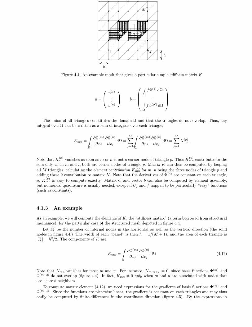
74 CHAPTER 4. FINITE ELEMENT METHODS FOR INCOMPRESSIBLE FLOW
9:9:9:9:9:9:9:99:9:9:9:9:9:9:99:9:9:9:9:9:9:99:9:9:9:9:9:9:99:9:9:9:9:9:9:99:9:9:9:9:9:9:99:9:9:9:9:9:9:99:9:9:9:9:9:9:9
;:;:;:;:;:;:;:;;:;:;:;:;:;:;:;;:;:;:;:;:;:;:;;:;:;:;:;:;:;:;;:;:;:;:;:;:;:;;:;:;:;:;:;:;:;;:;:;:;:;:;:;:;;:;:;:;:;:;:;:;
<:<:<:<:<:<:<:<<:<:<:<:<:<:<:<<:<:<:<:<:<:<:<<:<:<:<:<:<:<:<<:<:<:<:<:<:<:<<:<:<:<:<:<:<:<<:<:<:<:<:<:<:<<:<:<:<:<:<:<:<
=:=:=:=:=:=:=:==:=:=:=:=:=:=:==:=:=:=:=:=:=:==:=:=:=:=:=:=:==:=:=:=:=:=:=:==:=:=:=:=:=:=:==:=:=:=:=:=:=:==:=:=:=:=:=:=:=
PSfrag replacements
x, x1y, x2z, x3u, u1v, u2w, u3x1x2x 0i
ri(x 0i , t
)
ui(x 0i , t
)
P(t = 0
)
xu1
u2 > u1x1x2x3x 0i
ui dtdx 0
i
dui dtri(dt)
dri(dt)
P1
P2
x1x2x3R3
R2
R1
r3
r2
r1π2 + dϕ12
V (t)S (t)
V (t+∆t)− V (t)S (t+∆t)
un
V (t+∆t)
pT0, U0
TwLT0U0
Gradient fieldswi∂p∂xi
uiDivergence free vectorfields // to boundary
Lhx1x2
p0 > p1p1undS
u · n∆txyu0p0
η = y√4νtuu0
y = η√4νt
tηy
ωz =ω(η)·u0√
πνt
tLδ
ω ≈ 0U →y, vx, u
LUδu0
η = y√νx/u0
f ′ = uu0
Blasius profile
δ∗
xSeparation point
⇐= Pressure forcexy
luT
xy
dxdy
−dxdl = (dx, dy)
ndl = (dy,−dx)i− 1, j + 1
i, j + 1i+ 1, j + 1
cc′
bb′
i− 1, ji+ 1, j
i, jAabcd
dd′
aa′
i− 1, j − 1i, j − 1
i+ 1, j − 1j
ii+ 1ui,jvi,jpi,jpi,j
vi,j+1/2vi,j−1/2ui−1/2,ji− 1
2
ii+ 1
2
i+ 1i+ 3
2j + 1
2
jj − 1
2
j − 1ABC
u 32 ,1
v1, 32p1,1
012ij
InflowSolid wall
nΓ0Γ1Ω
M2
M
m m+ 2
1h
h
Figure 4.4: An example mesh that gives a particular simple stiffness matrix K
u =
u(1)
...u(n)
b =
∫
Ω
fΦ(1) dΩ
...∫
Ω
fΦ(N) dΩ
The union of all triangles constitutes the domain Ω and that the triangles do not overlap. Thus, anyintegral over Ω can be written as a sum of integrals over each triangle,
Kmn =
∫
Ω
∂Φ(m)
∂xj
∂Φ(n)
∂xjdΩ =
M∑
p=1
∫
Tp
∂Φ(m)
∂xj
∂Φ(n)
∂xjdΩ =
M∑
p=1
K(p)mn.
Note that K(p)mn vanishes as soon as m or n is not a corner node of triangle p. Thus K
(p)mn contributes to the
sum only when m and n both are corner nodes of triangle p. Matrix K can thus be computed by looping
all M triangles, calculating the element contribution K(p)mn for m, n being the three nodes of triangle p and
adding these 9 contribution to matrix K. Note that the derivatives of Φ(n) are constant on each triangle,
so K(p)mn is easy to compute exactly. Matrix C and vector b can also be computed by element assembly,
but numerical quadrature is usually needed, except if Uj and f happen to be particularly “easy” functions(such as constants).
4.1.3 An example
As an example, we will compute the elements of K, the “stiffness matrix” (a term borrowed from structuralmechanics), for the particular case of the structured mesh depicted in figure 4.4.
Let M be the number of internal nodes in the horizontal as well as the vertical direction (the solidnodes in figure 4.4.) The width of each “panel” is then h = 1/(M + 1), and the area of each triangle is|Tk| = h2/2. The components of K are
Kmn =
∫
Ω
∂Φ(m)
∂xj
∂Φ(n)
∂xjdΩ (4.12)
Note that Kmn vanishes for most m and n. For instance, Km,m+2 = 0, since basis functions Φ(m) andΦ(m+2) do not overlap (figure 4.4). In fact, Kmn 6= 0 only when m and n are associated with nodes thatare nearest neighbors.
To compute matrix element (4.12), we need expressions for the gradients of basis functions Φ(m) andΦ(m+1). Since the functions are piecewise linear, the gradient is constant on each triangles and may thuseasily be computed by finite-differences in the coordinate direction (figure 4.5). By the expressions in
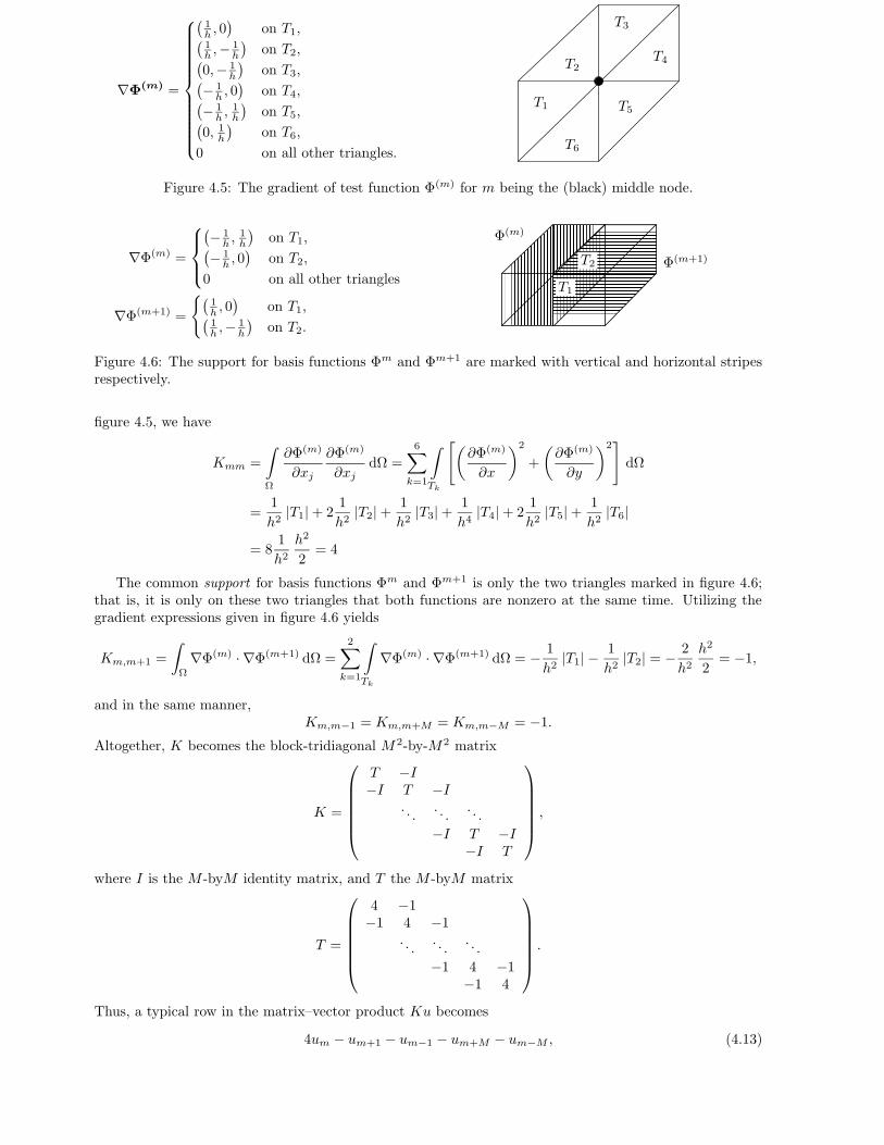
4.1. FEM FOR AN ADVECTION–DIFFUSION PROBLEM 75
∇Φ(m) =
(1h , 0)
on T1,(1h ,− 1
h
)on T2,
(0,− 1
h
)on T3,
(− 1h , 0)
on T4,(− 1h ,
1h
)on T5,
(0, 1h
)on T6,
0 on all other triangles.
PSfrag replacements
x, x1y, x2z, x3u, u1v, u2w, u3x1x2x 0i
ri(x 0i , t
)
ui(x 0i , t
)
P(t = 0
)
xu1
u2 > u1x1x2x3x 0i
ui dtdx 0
i
dui dtri(dt)
dri(dt)
P1
P2
x1x2x3R3
R2
R1
r3
r2
r1π2 + dϕ12
V (t)S (t)
V (t+∆t)− V (t)S (t+∆t)
un
V (t+∆t)
pT0, U0
TwLT0U0
Gradient fieldswi∂p∂xi
uiDivergence free vectorfields // to boundary
Lhx1x2
p0 > p1p1undS
u · n∆txyu0p0
η = y√4νtuu0
y = η√4νt
tηy
ωz =ω(η)·u0√
πνt
tLδ
ω ≈ 0U →y, vx, u
LUδu0
η = y√νx/u0
f ′ = uu0
Blasius profile
δ∗
xSeparation point
⇐= Pressure forcexy
luT
xy
dxdy
−dxdl = (dx, dy)
ndl = (dy,−dx)i− 1, j + 1
i, j + 1i+ 1, j + 1
cc′
bb′
i− 1, ji+ 1, j
i, jAabcd
dd′
aa′
i− 1, j − 1i, j − 1
i+ 1, j − 1j
ii+ 1ui,jvi,jpi,jpi,j
vi,j+1/2vi,j−1/2ui−1/2,ji− 1
2
ii+ 1
2
i+ 1i+ 3
2j + 1
2
jj − 1
2
j − 1ABC
u 32 ,1
v1, 32p1,1
012ij
InflowSolid wall
nΓ0Γ1Ω
M2
Mm
m+ 2
1h
T1
T2
T3
T4
T5
T6
Figure 4.5: The gradient of test function Φ(m) for m being the (black) middle node.
∇Φ(m) =
(− 1h ,
1h
)on T1,
(− 1h , 0)
on T2,
0 on all other triangles
∇Φ(m+1) =(
1h , 0)
on T1,(1h ,− 1
h
)on T2. >?>?>?>?>?>?>?>?>?>?>?>?>?>?>?>?>>?>?>?>?>?>?>?>?>?>?>?>?>?>?>?>?>>?>?>?>?>?>?>?>?>?>?>?>?>?>?>?>?>>?>?>?>?>?>?>?>?>?>?>?>?>?>?>?>?>>?>?>?>?>?>?>?>?>?>?>?>?>?>?>?>?>>?>?>?>?>?>?>?>?>?>?>?>?>?>?>?>?>>?>?>?>?>?>?>?>?>?>?>?>?>?>?>?>?>>?>?>?>?>?>?>?>?>?>?>?>?>?>?>?>?>
@?@?@?@?@?@?@?@?@?@?@?@?@?@?@?@@?@?@?@?@?@?@?@?@?@?@?@?@?@?@?@@?@?@?@?@?@?@?@?@?@?@?@?@?@?@?@@?@?@?@?@?@?@?@?@?@?@?@?@?@?@?@@?@?@?@?@?@?@?@?@?@?@?@?@?@?@?@@?@?@?@?@?@?@?@?@?@?@?@?@?@?@?@@?@?@?@?@?@?@?@?@?@?@?@?@?@?@?@@?@?@?@?@?@?@?@?@?@?@?@?@?@?@?@
A(A(A(A(A(A(A(A(AA(A(A(A(A(A(A(A(AA(A(A(A(A(A(A(A(AA(A(A(A(A(A(A(A(AA(A(A(A(A(A(A(A(AA(A(A(A(A(A(A(A(AA(A(A(A(A(A(A(A(AA(A(A(A(A(A(A(A(AA(A(A(A(A(A(A(A(AA(A(A(A(A(A(A(A(AA(A(A(A(A(A(A(A(AA(A(A(A(A(A(A(A(AA(A(A(A(A(A(A(A(AA(A(A(A(A(A(A(A(AA(A(A(A(A(A(A(A(AA(A(A(A(A(A(A(A(A
B(B(B(B(B(B(B(BB(B(B(B(B(B(B(BB(B(B(B(B(B(B(BB(B(B(B(B(B(B(BB(B(B(B(B(B(B(BB(B(B(B(B(B(B(BB(B(B(B(B(B(B(BB(B(B(B(B(B(B(BB(B(B(B(B(B(B(BB(B(B(B(B(B(B(BB(B(B(B(B(B(B(BB(B(B(B(B(B(B(BB(B(B(B(B(B(B(BB(B(B(B(B(B(B(BB(B(B(B(B(B(B(BB(B(B(B(B(B(B(B
PSfrag replacements
x, x1y, x2z, x3u, u1v, u2w, u3x1x2x 0i
ri(x 0i , t
)
ui(x 0i , t
)
P(t = 0
)
xu1
u2 > u1x1x2x3x 0i
ui dtdx 0
i
dui dtri(dt)
dri(dt)
P1
P2
x1x2x3R3
R2
R1
r3
r2
r1π2 + dϕ12
V (t)S (t)
V (t+∆t)− V (t)S (t+∆t)
un
V (t+∆t)
pT0, U0
TwLT0U0
Gradient fieldswi∂p∂xi
uiDivergence free vectorfields // to boundary
Lhx1x2
p0 > p1p1undS
u · n∆txyu0p0
η = y√4νtuu0
y = η√4νt
tηy
ωz =ω(η)·u0√
πνt
tLδ
ω ≈ 0U →y, vx, u
LUδu0
η = y√νx/u0
f ′ = uu0
Blasius profile
δ∗
xSeparation point
⇐= Pressure forcexy
luT
xy
dxdy
−dxdl = (dx, dy)
ndl = (dy,−dx)i− 1, j + 1
i, j + 1i+ 1, j + 1
cc′
bb′
i− 1, ji+ 1, j
i, jAabcd
dd′
aa′
i− 1, j − 1i, j − 1
i+ 1, j − 1j
ii+ 1ui,jvi,jpi,jpi,j
vi,j+1/2vi,j−1/2ui−1/2,ji− 1
2
ii+ 1
2
i+ 1i+ 3
2j + 1
2
jj − 1
2
j − 1ABC
u 32 ,1
v1, 32p1,1
012ij
InflowSolid wall
nΓ0Γ1Ω
M2
Mm
m+ 2
1h
T1
T2
Φ(m)
Φ(m+1)
Figure 4.6: The support for basis functions Φm and Φm+1 are marked with vertical and horizontal stripesrespectively.
figure 4.5, we have
Kmm =
∫
Ω
∂Φ(m)
∂xj
∂Φ(m)
∂xjdΩ =
6∑
k=1
∫
Tk
[(∂Φ(m)
∂x
)2
+
(∂Φ(m)
∂y
)2]
dΩ
=1
h2|T1|+ 2
1
h2|T2|+
1
h2|T3|+
1
h4|T4|+ 2
1
h2|T5|+
1
h2|T6|
= 81
h2h2
2= 4
The common support for basis functions Φm and Φm+1 is only the two triangles marked in figure 4.6;that is, it is only on these two triangles that both functions are nonzero at the same time. Utilizing thegradient expressions given in figure 4.6 yields
Km,m+1 =
∫
Ω
∇Φ(m) · ∇Φ(m+1) dΩ =2∑
k=1
∫
Tk
∇Φ(m) · ∇Φ(m+1) dΩ = − 1
h2|T1| −
1
h2|T2| = −
2
h2h2
2= −1,
and in the same manner,Km,m−1 = Km,m+M = Km,m−M = −1.
Altogether, K becomes the block-tridiagonal M 2-by-M2 matrix
K =
T −I−I T −I
. . .. . .
. . .
−I T −I−I T
,
where I is the M -byM identity matrix, and T the M -byM matrix
T =
4 −1−1 4 −1
. . .. . .
. . .
−1 4 −1−1 4
.
Thus, a typical row in the matrix–vector product Ku becomes
4um − um+1 − um−1 − um+M − um−M , (4.13)

76 CHAPTER 4. FINITE ELEMENT METHODS FOR INCOMPRESSIBLE FLOW
that is, after dividing expression (4.13) with h2, we recognize the classical five-point stencil for the negativeLaplacian −∇2.
Thus our finite-element discretization is for this particular mesh equivalent to a finite-volume or finite-difference discretization. However, for a general unstructured mesh, the finite-element discretization willnot give rise to any obvious finite-difference stencil.
4.1.4 Matrix properties and solvability
Matrix A is sparse: the elements of martix A are mostly zeros. At row m, matrix element Amn 6= 0 onlyin the columns where n represents a nearest neighbor to node m. The number of nonzero elements oneach row does not grow (on average) when the mesh is refined (since the number of nearest neighbors in amesh does not grow). Thus, the matrices become sparser and sparser as the mesh is refined. A commontechnique in finite-element codes is therefore to use sparse representation, that is, to store only the nonzeroelements and pointers to matrix locations.
It is immediate from expression (4.11) that Kmn = Knm, that is, K is a symmetric matrix (KT = K).Integration by parts also shows that matric C is skew symmetric (CT = −C).Theorem 1. K is positive definite, that is, vTKv > 0 for each v 6= 0.
Proof. Let vh ∈ Vh. Then vh =∑N
n=1 v(N)Φ(n). Denote v = (v(1), . . . , v(N))T .
vTKv =
N∑
m=1
N∑
n=1
v(n)∫
Ω
∂Φ(n)
∂xi
∂Φ(m)
∂xidΩ v(m)
=
∫
Ω
N∑
m=1
∂
∂xi
(
v(m)Φ(m)) N∑
n=1
∂
∂xi
(
v(m)Φ(n))
dΩ =
∫
Ω
∂vh∂xi
∂vh∂xi
dΩ ≥ 0,
with equality if and only if ∂vh
∂xi= 0, that is, if vh = Const. But since vh|Γ0 = 0, vh ≡ 0. ¤
From Theorem 1 also follows that A is positive definite. To see this, note that the skew-symmetry of Cyields that
vTCv =(vTCv
)T= vTCT v = −vTCv
that is, vTCv = 0 for each v. Thus
vTAv = vT (K + C) v = vTKv + vTCv = vTKv > 0
for each v 6= 0, that is, A is positive definite. However, A is not symmetric whenever Uj 6= 0.Recall that a linear system Au = b has a unique solution for each b if the matrix is nonsingular. A
positive-definite matrix is a particular example of a nonsingular matrix. We thus conclude that the linearsystem resulting from the finite-element discretization (4.7) has a unique solution.
4.1.5 Stability and accuracy
We have defined the finite-element approximation and showed that the finite-element approximation yieldsa linear system Au = b that has a unique solution. Now the question is whether the approximation is anygood. We will study the stability and accuracy of the numerical solution. FEM usually uses integral normsfor analysis of stability and accuracy. We start by reviewing some mathematical concepts that will be usedin the analysis.
Basic definitions and inequalities
The most basic integral norm is
‖v‖L2(Ω) =(∫
Ω
v2 dΩ
)1/2
For the current problem, a more fundamental quantity is the energy norm
‖v‖V =(∫
Ω
|∇v|2 dΩ)1/2
=
(∫
Ω
∂v
∂xi
∂v
∂xidΩ
)1/2
and associated inner product
(u, v)V =
∫
Ω
∇u · ∇v dΩ =∫
Ω
∂u
∂xi
∂v
∂xidΩ. (4.14)

4.1. FEM FOR AN ADVECTION–DIFFUSION PROBLEM 77
The Cauchy–Schwarz inequality for vectors a = (a1, . . . , an) is
|a · b| ≤ |a||b| = |a · a|1/2|b · b|1/2,
whereas for functions it reads
∣∣∣∣
∫
Ω
fg dΩ
∣∣∣∣≤(∫
Ω
f2 dΩ
)1/2(∫
Ω
g2 dΩ
)1/2
, (4.15)
which can be denoted(f, g)L2(Ω) ≤ ‖f‖L2(Ω)‖g‖L2(Ω).
The Cauchy–Schwarz inequality (4.15) implies that, for each nonzero, square-integrable g,
(∫
Ω
f2 dΩ
)1/2
≥∣∣∫
Ωfg dΩ
∣∣
(∫
Ωg2 dΩ
)1/2.
Choosing g = f yields equality in above expression. Thus
‖f‖L2(Ω) =(∫
Ω
f2 dΩ
)1/2
= maxg 6=0
∣∣∫
Ωfg dΩ
∣∣
(∫
Ωg2 dΩ
)1/2= max
g 6=0
∣∣∫
Ωfg dΩ
∣∣
‖g‖L2(Ω)
The rightmost expression is a “variational characterization” of the L2(Ω) norm, that is, it expresses thenorm in terms of something that is optimized. By inserting derivatives in the nominator and/or denominatorof the variational characterization, various exotic norms can be defined. A norm, different from the L2(Ω)norm and of importance for the Navier–Stokes equations is
‖p‖exotic = maxwi
∣∣∣∣
∫
Ω
p
(∂wi∂xi
)
dΩ
∣∣∣∣
(∫
Ω
|∇wi|2 dΩ)1/2
. (4.16)
This norm will be of crucial importance when we analyze the stability of FEM form the Navier–Stokesequations.
The Poincare inequality relates the energy and L2(Ω) norms:
Theorem 2 (Poincare inequality). There is a C > 0 such that
∫
Ω
v2 dΩ ≤ C
∫
Ω
∂v
∂xi
∂v
∂xidΩ,
that is,‖v‖2L2(Ω) ≤ C‖v‖2V
for each v ∈ V .
Remark 1. Theorem 2 says that the energy norm is stronger than then L2(Ω) norm. The smallest possiblevalue of C grows with the size of Ω. The Poincare inequality holds only if Ω is bounded in at least onedirection. Also, the inequality does not hold if
∫
Γ0dΓ = 0. However, the inequality
∫
Ω
v2 dΩ ≤ C
(∫
Ω
v2 dΩ +
∫
Ω
∂v
∂xi
∂v
∂xidΩ
)
holds also when∫
Γ0dΓ = 0.
Stability
Choosing vh = uh in equation (4.7) yields
∫
Ω
uhUj∂uh∂xj
dΩ + ν
∫
Ω
∂uh∂xj
∂uh∂xj
dΩ =
∫
Ω
fuh dΩ. (4.17)
Note that ∫
Ω
uhUj∂uh∂xj
dΩ = uTCu = 0,

78 CHAPTER 4. FINITE ELEMENT METHODS FOR INCOMPRESSIBLE FLOW
PSfrag replacements
x, x1y, x2z, x3u, u1v, u2w, u3x1x2x 0i
ri(x 0i , t
)
ui(x 0i , t
)
P(t = 0
)
xu1
u2 > u1x1x2x3x 0i
ui dtdx 0
i
dui dtri(dt)
dri(dt)
P1
P2
x1x2x3R3
R2
R1
r3
r2
r1π2 + dϕ12
V (t)S (t)
V (t+∆t)− V (t)S (t+∆t)
un
V (t+∆t)
pT0, U0
TwLT0U0
Gradient fieldswi∂p∂xi
uiDivergence free vectorfields // to boundary
Lhx1x2
p0 > p1p1undS
u · n∆txyu0p0
η = y√4νtuu0
y = η√4νt
tηy
ωz =ω(η)·u0√
πνt
tLδ
ω ≈ 0U →y, vx, u
LUδu0
η = y√νx/u0
f ′ = uu0
Blasius profile
δ∗
xSeparation point
⇐= Pressure forcexy
luT
xy
dxdy
−dxdl = (dx, dy)
ndl = (dy,−dx)i− 1, j + 1
i, j + 1i+ 1, j + 1
cc′
bb′
i− 1, ji+ 1, j
i, jAabcd
dd′
aa′
i− 1, j − 1i, j − 1
i+ 1, j − 1j
ii+ 1ui,jvi,jpi,jpi,j
vi,j+1/2vi,j−1/2ui−1/2,ji− 1
2
ii+ 1
2
i+ 1i+ 3
2j + 1
2
jj − 1
2
j − 1ABC
u 32 ,1
v1, 32p1,1
012ij
InflowSolid wall
nΓ0Γ1Ω
M2
Mm
m+ 2
1h
V
Vh
u
uh
Figure 4.7: An orthogonal projection on a line. Note that the vector u − uh is the shortest of all vectorsu− vh for vh ∈ Vh, that is, ‖u− uh‖ ≤ ‖u− vh‖ ∀vh ∈ Vh.
since C = −CT (using the notation of § 4.1.4).Expression (4.17) thus becomes
ν
∫
Ω
∂uh∂xi
∂uh∂xi
dΩ
︸ ︷︷ ︸
‖uh‖2V
=
∫
Ω
fuh dΩ
(Cauchy–Schwarz) ≤(∫
Ω
f2 dΩ
)1/2(∫
Ω
u2h dΩ
)1/2
(Poincare) ≤ C
(∫
Ω
f2 dΩ
)1/2(∫
Ω
∂uh∂xi
∂uh∂xi
dΩ
)1/2
≤ C‖f‖L2(Ω)‖uh‖V .
Dividing with ‖uh‖V shows that‖uh‖V ≤
C
ν‖f‖L2(Ω)
where the constant C does not depend on h. That is, we have shown that uh cannot blow up as thediscretization is refined, which is the same as saying that the numerical solution is stable.
Error bounds
Choosing v = vh ∈ Vh ⊂ V in variational problem (4.6) and subtracting equation (4.7) from(4.6) yields the“Galerkin orthogonality”,
ν
∫
Ω
∂vh∂xi
∂
∂xi(u− uh) dΩ +
∫
Ω
vhUj∂
∂xj(u− uh) dΩ = 0 ∀vh ∈ Vh.
This is a “true” orthogonality condition when Uj ≡ 0:
ν
∫
Ω
∂vh∂xi
∂
∂xi(u− uh) dΩ = 0 ∀vh ∈ Vh; (4.18)
that is, the error u − uh is orthogonal to each vh ∈ Vh with respect to the inner product (4.14). Cf. twoorthogonal vectors: a · b = 0 . Orthogonality relation (4.18) means that uh is an orthogonal projectionof u on Vh. As illustrated in figure 4.7, the orthogonal projection on a subspace yields the vector that isclosest to the given element in the norm derived from the inner product in which orthogonality is defined.Orthogonality property (4.18) (cf. figure 4.7) implies that the FE approximation is optimal in the energynorm when Ui ≡ 0:
‖u− uh‖V ≤ ‖u− vh‖V ∀vh ∈ Vh. (4.19)
The matrix A is symmetric in this case (since C = 0).When Uj 6= 0, the FEM approximation is no longer optimal in this sense. However, there is a C > 0
such that Cea’s lemma holds,
‖u− uh‖V ≤C
ν‖u− vh‖V ∀vh ∈ Vh. (4.20)
Matrix A is nonsymmetric in this case. Note that the approximation may be far from optimal when ν issmall, as the next example illustrates.

4.1. FEM FOR AN ADVECTION–DIFFUSION PROBLEM 79
0.9 0.92 0.94 0.96 0.98
0.1
0.2
0.3
0.4
0.5
0.6
0.7
0.8
PSfrag replacements
x, x1y, x2z, x3u, u1v, u2w, u3x1x2x 0i
ri(x 0i , t
)
ui(x 0i , t
)
P(t = 0
)
xu1
u2 > u1x1x2x3x 0i
ui dtdx 0
i
dui dtri(dt)
dri(dt)
P1
P2
x1x2x3R3
R2
R1
r3
r2
r1π2 + dϕ12
V (t)S (t)
V (t+∆t)− V (t)S (t+∆t)
un
V (t+∆t)
pT0, U0
TwLT0U0
Gradient fieldswi∂p∂xi
uiDivergence free vectorfields // to boundary
Lhx1x2
p0 > p1p1undS
u · n∆txyu0p0
η = y√4νtuu0
y = η√4νt
tηy
ωz =ω(η)·u0√
πνt
tLδ
ω ≈ 0U →y, vx, u
LUδu0
η = y√νx/u0
f ′ = uu0
Blasius profile
δ∗
xSeparation point
⇐= Pressure forcexy
luT
xy
dxdy
−dxdl = (dx, dy)
ndl = (dy,−dx)i− 1, j + 1
i, j + 1i+ 1, j + 1
cc′
bb′
i− 1, ji+ 1, j
i, jAabcd
dd′
aa′
i− 1, j − 1i, j − 1
i+ 1, j − 1j
ii+ 1ui,jvi,jpi,jpi,j
vi,j+1/2vi,j−1/2ui−1/2,ji− 1
2
ii+ 1
2
i+ 1i+ 3
2j + 1
2
jj − 1
2
j − 1ABC
u 32 ,1
v1, 32p1,1
0
12ij
InflowSolid wall
nΓ0Γ1Ω
M2
Mm
m+ 2
1
hVVhuuh
u
x
Figure 4.8: Under-resolved standard Galerkin finite-element approximations may yield oscillations foradvection-dominated flows.
PSfrag replacements
x, x1y, x2z, x3u, u1v, u2w, u3x1x2x 0i
ri(x 0i , t
)
ui(x 0i , t
)
P(t = 0
)
xu1
u2 > u1x1x2x3x 0i
ui dtdx 0
i
dui dtri(dt)
dri(dt)
P1
P2
x1x2x3R3
R2
R1
r3
r2
r1π2 + dϕ12
V (t)S (t)
V (t+∆t)− V (t)S (t+∆t)
un
V (t+∆t)
pT0, U0
TwLT0U0
Gradient fieldswi∂p∂xi
uiDivergence free vectorfields // to boundary
Lhx1x2
p0 > p1p1undS
u · n∆txyu0p0
η = y√4νtuu0
y = η√4νt
tηy
ωz =ω(η)·u0√
πνt
tLδ
ω ≈ 0U →y, vx, u
LUδu0
η = y√νx/u0
f ′ = uu0
Blasius profile
δ∗
xSeparation point
⇐= Pressure forcexy
luT
xy
dxdy
−dxdl = (dx, dy)
ndl = (dy,−dx)i− 1, j + 1
i, j + 1i+ 1, j + 1
cc′
bb′
i− 1, ji+ 1, j
i, jAabcd
dd′
aa′
i− 1, j − 1i, j − 1
i+ 1, j − 1j
ii+ 1ui,jvi,jpi,jpi,j
vi,j+1/2vi,j−1/2ui−1/2,ji− 1
2
ii+ 1
2
i+ 1i+ 3
2j + 1
2
jj − 1
2
j − 1ABC
u 32 ,1
v1, 32
v1, 32
p1,1
012ij
InflowSolid wall
nΓ0Γ1Ω
M2
Mm
m+ 2
1
hVVhuuh
Figure 4.9: An interpolant Πhv interpolates v at the nodal points.
Example 1. Let us consider the above FEM applied to the 1D problem
− 1
500u′′ + u′ = 1 in (0, 1).
u(0) = u(1) = 0(4.21)
The problem is advection dominated, that is, the viscosity coefficient in equation (4.21) is quite small:ν = 1/500. A boundary layer with sharp gradients forms close to x = 1. The solid line in figure 4.8 showsthe FE solution h = 1/1000, whereas the dashed line shows the FE approximation for h = 1/200. ¤
The result of example 1 is typical: under-resolved standard Galerkin methods may generate oscillationsfor advection-dominated flows in areas of sharp gradients.
An explanation of this phenomenon is that the directions of flow is not accounted for in the standardGalerkin approximation. Galerkin approximations correspond to finite-difference central schemes. Upwind-ing is used to prevent oscillations for finite-difference methods. Various methods exist to obtain similareffects in FEM, for instance streamline diffusion and discontinuous Galerkin. Both these methods modifythe basic Galerkin idea to account for flow-direction effects.
Approximation and mesh quality
Estimates (4.19) and (4.20) are independent of the choice of Vh! We only used that Vh ⊂ V . Next stepin assessing the error is an approximation problem: How well can functions in Vh approximate those inV ? This step is independent of the equation in question. Interpolants are used to study approximationproperties. The interpolant is the function Πhv ∈ Vh that interpolates the function v ∈ V at the nodepoints of the triangulation, as illustrated for a 1D case in figure 4.9.
Approximation theory yields that, for sufficiently smooth v,
‖v −Πhv‖L2(Ω) ≤ Ch2 “second order error”
‖v −Πhv‖V ≤ Ch “first order error”(4.22)
The constant C contains integrals of the second derivatives of v.
Amesh quality assumption is needed for (4.22) to hold. The essential point is: beware of “thin” triangles;do not let the shape deteriorate as the mesh is refined. A strategy to preserve mesh quality when refiningis to subdivide each triangle into four new triangles by joining the edge midpoints (figure 4.10).
Each of the conditions below is sufficient for approximation property (4.22) to hold:

80 CHAPTER 4. FINITE ELEMENT METHODS FOR INCOMPRESSIBLE FLOW
PSfrag replacements
x, x1y, x2z, x3u, u1v, u2w, u3x1x2x 0i
ri(x 0i , t
)
ui(x 0i , t
)
P(t = 0
)
xu1
u2 > u1x1x2x3x 0i
ui dtdx 0
i
dui dtri(dt)
dri(dt)
P1
P2
x1x2x3R3
R2
R1
r3
r2
r1π2 + dϕ12
V (t)S (t)
V (t+∆t)− V (t)S (t+∆t)
un
V (t+∆t)
pT0, U0
TwLT0U0
Gradient fieldswi∂p∂xi
uiDivergence free vectorfields // to boundary
Lhx1x2
p0 > p1p1undS
u · n∆txyu0p0
η = y√4νtuu0
y = η√4νt
tηy
ωz =ω(η)·u0√
πνt
tLδ
ω ≈ 0U →y, vx, u
LUδu0
η = y√νx/u0
f ′ = uu0
Blasius profile
δ∗
xSeparation point
⇐= Pressure forcexy
luT
xy
dxdy
−dxdl = (dx, dy)
ndl = (dy,−dx)i− 1, j + 1
i, j + 1i+ 1, j + 1
cc′
bb′
i− 1, ji+ 1, j
i, jAabcd
dd′
aa′
i− 1, j − 1i, j − 1
i+ 1, j − 1j
ii+ 1ui,jvi,jpi,jpi,j
vi,j+1/2vi,j−1/2ui−1/2,ji− 1
2
ii+ 1
2
i+ 1i+ 3
2j + 1
2
jj − 1
2
j − 1ABC
u 32 ,1
v1, 32p1,1
012ij
InflowSolid wall
nΓ0Γ1Ω
M2
Mm
m+ 2
1hVVhuuh
Figure 4.10: A subdivision that preserves mesh quality.
(i) (“Maximum angle condition”). The largest an-gle of any triangle should not approach 180 ash→ 0.
(ii) (“Chunkiness parameter condition”). Thequotient between the diameter of the largestcircle that can be inscribed and the diameterof the triangle should not vanish as h→ 0.
PSfrag replacements
x, x1y, x2z, x3u, u1v, u2w, u3x1x2x 0i
ri(x 0i , t
)
ui(x 0i , t
)
P(t = 0
)
xu1
u2 > u1x1x2x3x 0i
ui dtdx 0
i
dui dtri(dt)
dri(dt)
P1
P2
x1x2x3R3
R2
R1
r3
r2
r1π2 + dϕ12
V (t)S (t)
V (t+∆t)− V (t)S (t+∆t)
un
V (t+∆t)
pT0, U0
TwLT0U0
Gradient fieldswi∂p∂xi
uiDivergence free vectorfields // to boundary
Lhx1x2
p0 > p1p1undS
u · n∆txyu0p0
η = y√4νtuu0
y = η√4νt
tηy
ωz =ω(η)·u0√
πνt
tLδ
ω ≈ 0U →y, vx, u
LUδu0
η = y√νx/u0
f ′ = uu0
Blasius profile
δ∗
xSeparation point
⇐= Pressure forcexy
luT
xy
dxdy
−dxdl = (dx, dy)
ndl = (dy,−dx)i− 1, j + 1
i, j + 1i+ 1, j + 1
cc′
bb′
i− 1, ji+ 1, j
i, jAabcd
dd′
aa′
i− 1, j − 1i, j − 1
i+ 1, j − 1j
ii+ 1ui,jvi,jpi,jpi,j
vi,j+1/2vi,j−1/2ui−1/2,ji− 1
2
ii+ 1
2
i+ 1i+ 3
2j + 1
2
jj − 1
2
j − 1ABC
u 32 ,1
v1, 32p1,1
012ij
InflowSolid wall
nΓ0Γ1Ω
M2
Mm
m+ 2
1hVVhuuh
Condition (ii) implies (i), but not the reverse.
Accuracy of the FE solution
Error bounds (4.19) and (4.20) together with approximation property (4.22) implies
‖u− uh‖V ≤ Ch
Further analysis (not provided here) yields
‖u− uh‖L2(Ω) ≤ Ch2.
This second-order convergence rate requires a mesh quality assumption and a sufficiently smooth solution u(since the constant C contains second derivatives of u). The convergence rate is of optimal order : it agreeswith approximation property (4.22) and is the best order that in general can be obtained for, in this case,piecewise-linear functions. However, the solution may still be bad for a particular, too-crude mesh; recallexample 1.
Improving Accuracy
Accuracy is improved by refining the mesh (“h-method”). This may be done adaptively, where it is needed(say, in areas of large gradients), to prevent the matrices to become too large. Automatic methods foradaptation are common.
An alternative is to keep the mesh fixed and increase the order of the polynomials at each triangle(“p-method”). For instance, continuous, piecewise quadratics yields a third-order-accurate solution (in theL2(Ω) norm).
These strategies may be combined in the “h–p method”, where the mesh is refined in certain regionsand the order of approximations is increased in other.
4.1.6 Alternative Elements, 3D
A quadrilateral is a “skewed” rectangle: four points connected by straight lines to form a closed geometricobject. Nonoverlapping quadrilaterals can be used to “triangulate” a domain, as in figure 4.11.
An example of a finite-element space Vh on quadrilaterals is globally continuous functions varying linearlyalong the edges. As in the triangular case, the functions are defined uniquely by specifying the functionvalues at each node. The functions are defined by interpolation into the interior of each quadrilateral. Thisspace reduces to piecewise bilinear functions for rectangles with edges in the coordinate directions:
vh(x, y) = a+ b x+ c y + d xy
Quadrilaterals on a “logically rectangular domain” (a distorted rectangle, as in figure 4.11) yields a regularstructure to the matrix A. This may

4.1. FEM FOR AN ADVECTION–DIFFUSION PROBLEM 81
PSfrag replacements
x, x1y, x2z, x3u, u1v, u2w, u3x1x2x 0i
ri(x 0i , t
)
ui(x 0i , t
)
P(t = 0
)
xu1
u2 > u1x1x2x3x 0i
ui dtdx 0
i
dui dtri(dt)
dri(dt)
P1
P2
x1x2x3R3
R2
R1
r3
r2
r1π2 + dϕ12
V (t)S (t)
V (t+∆t)− V (t)S (t+∆t)
un
V (t+∆t)
pT0, U0
TwLT0U0
Gradient fieldswi∂p∂xi
uiDivergence free vectorfields // to boundary
Lhx1x2
p0 > p1p1undS
u · n∆txyu0p0
η = y√4νtuu0
y = η√4νt
tηy
ωz =ω(η)·u0√
πνt
tLδ
ω ≈ 0U →y, vx, u
LUδu0
η = y√νx/u0
f ′ = uu0
Blasius profile
δ∗
xSeparation point
⇐= Pressure forcexy
luT
xy
dxdy
−dxdl = (dx, dy)
ndl = (dy,−dx)i− 1, j + 1
i, j + 1i+ 1, j + 1
cc′
bb′
i− 1, ji+ 1, j
i, jAabcd
dd′
aa′
i− 1, j − 1i, j − 1
i+ 1, j − 1j
ii+ 1ui,jvi,jpi,jpi,j
vi,j+1/2vi,j−1/2ui−1/2,ji− 1
2
ii+ 1
2
i+ 1i+ 3
2j + 1
2
jj − 1
2
j − 1ABC
u 32 ,1
v1, 32p1,1
012ij
InflowSolid wall
nΓ0Γ1Ω
M2
Mm
m+ 2
1hVVhuuh
Figure 4.11: A logically rectangular domain triangulated with quadrilaterals.
PSfrag replacements
x, x1y, x2z, x3u, u1v, u2w, u3x1x2x 0i
ri(x 0i , t
)
ui(x 0i , t
)
P(t = 0
)
xu1
u2 > u1x1x2x3x 0i
ui dtdx 0
i
dui dtri(dt)
dri(dt)
P1
P2
x1x2x3R3
R2
R1
r3
r2
r1π2 + dϕ12
V (t)S (t)
V (t+∆t)− V (t)S (t+∆t)
un
V (t+∆t)
pT0, U0
TwLT0U0
Gradient fieldswi∂p∂xi
uiDivergence free vectorfields // to boundary
Lhx1x2
p0 > p1p1undS
u · n∆txyu0p0
η = y√4νtuu0
y = η√4νt
tηy
ωz =ω(η)·u0√
πνt
tLδ
ω ≈ 0U →y, vx, u
LUδu0
η = y√νx/u0
f ′ = uu0
Blasius profile
δ∗
xSeparation point
⇐= Pressure forcexy
luT
xy
dxdy
−dxdl = (dx, dy)
ndl = (dy,−dx)i− 1, j + 1
i, j + 1i+ 1, j + 1
cc′
bb′
i− 1, ji+ 1, j
i, jAabcd
dd′
aa′
i− 1, j − 1i, j − 1
i+ 1, j − 1j
ii+ 1ui,jvi,jpi,jpi,j
vi,j+1/2vi,j−1/2ui−1/2,ji− 1
2
ii+ 1
2
i+ 1i+ 3
2j + 1
2
jj − 1
2
j − 1ABC
u 32 ,1
v1, 32p1,1
012ij
InflowSolid wall
nΓ0Γ1Ω
M2
Mm
m+ 2
1hVVhuuh
Figure 4.12: In 3D, triangular and quadrilateral elements generalize to tetrahedral (left) and hexahedral(right) meshes.
• give high accuracy (particularly if the mesh is aligned with the flow), and
• allow efficient solution of the linear system (particularly for uniform, rectangular meshes).
Compared to triangular mesh, it is harder to generate quadrilateral meshes automatically for compli-cated geometries.
Triangular and quadrilateral meshes generalize in 3D to tetrahedral and hexahedral meshes (figure 4.12).Advantages and limitations with tetrahedral and hexahedral meshes are similar to corresponding meshesin 2D.

82 CHAPTER 4. FINITE ELEMENT METHODS FOR INCOMPRESSIBLE FLOW
C:C:C:C:C:C:C:C:C:C:C:C:C:C:C:C:C:C:C:C:C:C:C:C:C:C:C:C:C:C:C:C:C:C:C:C:C:C:C:C:CD:D:D:D:D:D:D:D:D:D:D:D:D:D:D:D:D:D:D:D:D:D:D:D:D:D:D:D:D:D:D:D:D:D:D:D:D:D:D:D:D
E:E:E:E:E:E:E:E:E:E:E:E:E:E:E:E:E:E:E:E:E:E:E:E:E:E:E:E:E:E:E:E:E:E:E:E:E:E:E:E:EE:E:E:E:E:E:E:E:E:E:E:E:E:E:E:E:E:E:E:E:E:E:E:E:E:E:E:E:E:E:E:E:E:E:E:E:E:E:E:E:EE:E:E:E:E:E:E:E:E:E:E:E:E:E:E:E:E:E:E:E:E:E:E:E:E:E:E:E:E:E:E:E:E:E:E:E:E:E:E:E:EE:E:E:E:E:E:E:E:E:E:E:E:E:E:E:E:E:E:E:E:E:E:E:E:E:E:E:E:E:E:E:E:E:E:E:E:E:E:E:E:EE:E:E:E:E:E:E:E:E:E:E:E:E:E:E:E:E:E:E:E:E:E:E:E:E:E:E:E:E:E:E:E:E:E:E:E:E:E:E:E:EE:E:E:E:E:E:E:E:E:E:E:E:E:E:E:E:E:E:E:E:E:E:E:E:E:E:E:E:E:E:E:E:E:E:E:E:E:E:E:E:EE:E:E:E:E:E:E:E:E:E:E:E:E:E:E:E:E:E:E:E:E:E:E:E:E:E:E:E:E:E:E:E:E:E:E:E:E:E:E:E:EE:E:E:E:E:E:E:E:E:E:E:E:E:E:E:E:E:E:E:E:E:E:E:E:E:E:E:E:E:E:E:E:E:E:E:E:E:E:E:E:EE:E:E:E:E:E:E:E:E:E:E:E:E:E:E:E:E:E:E:E:E:E:E:E:E:E:E:E:E:E:E:E:E:E:E:E:E:E:E:E:EE:E:E:E:E:E:E:E:E:E:E:E:E:E:E:E:E:E:E:E:E:E:E:E:E:E:E:E:E:E:E:E:E:E:E:E:E:E:E:E:E
F:F:F:F:F:F:F:F:F:F:F:F:F:F:F:F:F:F:F:F:F:F:F:F:F:F:F:F:F:F:F:F:F:F:F:F:F:F:F:F:FF:F:F:F:F:F:F:F:F:F:F:F:F:F:F:F:F:F:F:F:F:F:F:F:F:F:F:F:F:F:F:F:F:F:F:F:F:F:F:F:FF:F:F:F:F:F:F:F:F:F:F:F:F:F:F:F:F:F:F:F:F:F:F:F:F:F:F:F:F:F:F:F:F:F:F:F:F:F:F:F:FF:F:F:F:F:F:F:F:F:F:F:F:F:F:F:F:F:F:F:F:F:F:F:F:F:F:F:F:F:F:F:F:F:F:F:F:F:F:F:F:FF:F:F:F:F:F:F:F:F:F:F:F:F:F:F:F:F:F:F:F:F:F:F:F:F:F:F:F:F:F:F:F:F:F:F:F:F:F:F:F:FF:F:F:F:F:F:F:F:F:F:F:F:F:F:F:F:F:F:F:F:F:F:F:F:F:F:F:F:F:F:F:F:F:F:F:F:F:F:F:F:FF:F:F:F:F:F:F:F:F:F:F:F:F:F:F:F:F:F:F:F:F:F:F:F:F:F:F:F:F:F:F:F:F:F:F:F:F:F:F:F:FF:F:F:F:F:F:F:F:F:F:F:F:F:F:F:F:F:F:F:F:F:F:F:F:F:F:F:F:F:F:F:F:F:F:F:F:F:F:F:F:FF:F:F:F:F:F:F:F:F:F:F:F:F:F:F:F:F:F:F:F:F:F:F:F:F:F:F:F:F:F:F:F:F:F:F:F:F:F:F:F:FF:F:F:F:F:F:F:F:F:F:F:F:F:F:F:F:F:F:F:F:F:F:F:F:F:F:F:F:F:F:F:F:F:F:F:F:F:F:F:F:F
PSfrag replacements
x, x1y, x2z, x3u, u1v, u2w, u3x1x2x 0i
ri(x 0i , t
)
ui(x 0i , t
)
P(t = 0
)
xu1
u2 > u1x1x2x3x 0i
ui dtdx 0
i
dui dtri(dt)
dri(dt)
P1
P2
x1x2x3R3
R2
R1
r3
r2
r1π2 + dϕ12
V (t)S (t)
V (t+∆t)− V (t)S (t+∆t)
un
V (t+∆t)
pT0, U0
TwLT0U0
Gradient fieldswi∂p∂xi
uiDivergence free vectorfields // to boundary
Lhx1x2
p0 > p1p1undS
u · n∆txyu0p0
η = y√4νtuu0
y = η√4νt
tηy
ωz =ω(η)·u0√
πνt
tLδ
ω ≈ 0U →y, vx, u
LUδu0
η = y√νx/u0
f ′ = uu0
Blasius profile
δ∗
xSeparation point
⇐= Pressure forcexy
luT
xy
dxdy
−dxdl = (dx, dy)
ndl = (dy,−dx)i− 1, j + 1
i, j + 1i+ 1, j + 1
cc′
bb′
i− 1, ji+ 1, j
i, jAabcd
dd′
aa′
i− 1, j − 1i, j − 1
i+ 1, j − 1j
ii+ 1ui,jvi,jpi,jpi,j
vi,j+1/2vi,j−1/2ui−1/2,ji− 1
2
ii+ 1
2
i+ 1i+ 3
2j + 1
2
jj − 1
2
j − 1ABC
u 32 ,1
v1, 32p1,1
012ij
InflowSolid wall
nΓ0Γ1Ω
M2
Mm
m+ 2
1hVVhuuh
Γ0
Γ0
Γ0
Γ1Ω
Figure 4.13: A simple example of a domain.
G G GH H I IJ J K KL L M MN NO OP PQ QR RS ST TU UV VW WX XY YZ Z
[ [\ \] ]^ ^ _ _` ` a ab b
c cd de ef f
PSfrag replacements
x, x1y, x2z, x3u, u1v, u2w, u3x1x2x 0i
ri(x 0i , t
)
ui(x 0i , t
)
P(t = 0
)
xu1
u2 > u1x1x2x3x 0i
ui dtdx 0
i
dui dtri(dt)
dri(dt)
P1
P2
x1x2x3R3
R2
R1
r3
r2
r1π2 + dϕ12
V (t)S (t)
V (t+∆t)− V (t)S (t+∆t)
un
V (t+∆t)
pT0, U0
TwLT0U0
Gradient fieldswi∂p∂xi
uiDivergence free vectorfields // to boundary
Lhx1x2
p0 > p1p1undS
u · n∆txyu0p0
η = y√4νtuu0
y = η√4νt
tηy
ωz =ω(η)·u0√
πνt
tLδ
ω ≈ 0U →y, vx, u
LUδu0
η = y√νx/u0
f ′ = uu0
Blasius profile
δ∗
xSeparation point
⇐= Pressure forcexy
luT
xy
dxdy
−dxdl = (dx, dy)
ndl = (dy,−dx)i− 1, j + 1
i, j + 1i+ 1, j + 1
cc′
bb′
i− 1, ji+ 1, j
i, jAabcd
dd′
aa′
i− 1, j − 1i, j − 1
i+ 1, j − 1j
ii+ 1ui,jvi,jpi,jpi,j
vi,j+1/2vi,j−1/2ui−1/2,ji− 1
2
ii+ 1
2
i+ 1i+ 3
2j + 1
2
jj − 1
2
j − 1ABC
u 32 ,1
v1, 32p1,1
012ij
InflowSolid wall
nΓ0Γ1Ω
M2
Mm
m+ 2
1hVVhuuhΓ0Γ1Ω
Γ0
Γ0 Γ0
Γ0
Figure 4.14: The black nodes are the degrees of freedom for the velocity components, which are fewer thanthe number of triangles.
4.2 FEM for Navier–Stokes
We now turn to the Navier–Stokes equations for the steady flow of an incompressible fluid, and considera situation with flow in a bounded domain Ω. A simple example domain is depicted in figure 4.13. Themathematical problem in differential form is
uj∂ui∂xj
+∂p
∂xi− 1
Re∇2ui = fi in Ω, (4.23a)
∂ui∂xi
= 0 in Ω. (4.23b)
ui = gi on Γ0 (4.23c)
− 1
Re
∂ui∂xj
nj + pni = 0 on Γ1. (4.23d)
The boundary condition on Γ1 = ∂Ω \ Γ0 is of no obvious physical significance, but is useful as anartificial outflow condition.
The Navier–Stokes equations is a system of nonlinear advection–diffusion equations together withthe incompressibility condition (4.23b). This condition introduces new complications not present in theadvection–diffusion problem of section 4.1. Naive approximations of the Navier–Stokes equations are boundto produce disappoing results, as the following example indicates.
Example 2 (“the counting argument”). Consider a case with only Dirichlet boundary conditions—that is,Γ1 = ∅—and the mesh of figure 4.14. Assume that we use continuous, piecewise-linear approximations uh,vh for the x- and y-components of the velocity field. There are I number of panels in each direction andtherefore 2(I − 1)2 degrees of freedom (two times the number of black dots) for the velocity vector field.The left side of equation (4.23b), that is
∂uh∂x
+∂vh∂y
is here constant on each triangle. Thus, demanding equation (4.23b) to be satisfied on each triangle yields2I2 equations, which is more than the degrees of freedom for the velocity ! Thus uh = vh = 0 is the only FEfunction satisfying the incompressibility condition (4.23b)! ¤

4.2. FEM FOR NAVIER–STOKES 83
Following strategies can be used to tackle the problem of example 2.
(i) Use more degrees of freedom for the velocity—for instance continuous, piecewise quadratics on eachtriangle—to balance the large number of equations associated with the incompressibility condition.
(ii) Accept that the discrete velocities only is approximately divergence-free.
(iii) Associate the velocity with the midpoints of edges instead of the vertices. This also gives more degreesof freedom for the velocities. (There are ∼ 3I2 edges, but only ∼ 2I2 vertices).
Strategies (i) and (ii) are the “standard” methods, whereas (iii) leads to “non-conforming” approxima-tions related to finite-difference and finite-volume approximation with “staggered mesh”.
4.2.1 A variational form of the Navier–Stokes equations
To derive the variational form, we need new integration-by-part formulas. The product rule of differentiationyields
∂
∂xj
(
zi∂ui∂xj
)
=∂zi∂xj
∂ui∂xj
+ zi∇2ui (4.24)
and∂
∂xj(zjp) = zi
∂p
∂xi+ p
∂zj∂xj
. (4.25)
Integrating expressions (4.24) and (4.25) and applying the the divergence theorem (4.3) on the left sidesyields ∫
Γ
njzi∂ui∂xj
dΓ =
∫
Ω
∂zi∂xj
∂ui∂xj
dΩ +
∫
Ω
zi∇2ui dΩ (4.26)
and ∫
Γ
njzjpdΓ =
∫
Ω
zi∂p
∂xidΩ +
∫
Ω
p∂zi∂xi
dΩ, (4.27)
which are the integration-by-parts formulas needed to derive our variational form.Now, let zi be a smooth vector-valued function on Ω that vanishes on Γ0. Multiply both sides of
equation (4.23a) with zi, integrating over Ω, and utilizing (4.26) and (4.27), we find that
∫
Ω
zifi dΩ =
∫
Ω
ziuj∂ui∂xj
dΩ +
∫
Ω
zi∂p
∂xidΩ− 1
Re
∫
Ω
zi∇2ui dΩ
=
∫
Ω
ziuj∂ui∂xj
dΩ +1
Re
∫
Ω
∂zi∂xj
∂ui∂xj
dΩ− 1
Re
∫
Γ
njzi∂ui∂xj
dΓ−∫
Ω
p∂zi∂xi
dΩ +
∫
Γ
njzjpdΓ
=
∫
Ω
ziuj∂ui∂xj
dΩ +1
Re
∫
Ω
∂zi∂xj
∂ui∂xj
dΩ−∫
Ω
p∂zi∂xi
dΩ,
(4.28)
where, in the last equality, the boundary integrals vanish on Γ0 since zi = 0 on Γ0 and on Γ1 due to boundarycondition (4.23d). Moreover, multiplying equation (4.23b) with a smooth function q and integrating yields
∫
Ω
q∂ui∂xi
dΩ = 0 (4.29)
Thus, we conclude that a classical solution (a twice continuously differentiable solution) to the Navier–Stokes equations satisfies the variational forms (4.28) and (4.29) for all smooth functions zi and q such thatzi vanishes on Γ0.
Similarly as for the advection–diffusion problem, the variational form will be used to define weak solu-tions, without explicit reference to the differential equations. A difference with advection–diffusion problemis that we here need different function spaces for the velocity components and the pressure. Also note thatui = gi on Γ0 whereas zi vanishes on Γ0. To avoid this last complication and simplify the exposition, wewill only consider homogeneous boundary conditions, gi = 0. Thus, the equations will be “driven” only bythe right-hand side fi, which, for instance, could be gravity or magnetic forcing for a electrically conductingfluid.
The pressure space is
H = L2(Ω) =
q |∫
Ω
q2 dΩ < +∞
,
84 CHAPTER 4. FINITE ELEMENT METHODS FOR INCOMPRESSIBLE FLOW
and the space of velocity components is
V =
u |∫
Ω
∂u
∂xi
∂u
∂xidΩ < +∞ and u = 0 on Γ0
.
For the analysis in section 4.2.4, it will be convenient to work with the space V of the velocity vectoru = (u1, u2). Saying that u ∈ V is equivalent to saying that that each velocity component ui ∈ V . Theenergy norm for elements of V is denoted
‖u‖V =
(∫
Ω
∂ui∂xj
∂ui∂xj
dΩ
)1/2
,
whereas the L2(Ω) norm is
‖u‖L2(Ω) =(∫
Ω
uiui dΩ
)1/2
.
We assume that both boundary conditions really are active. In the case of only Dirichlet boundarycondition, that is, that Γ0 constitute the whole boundary, the pressure is only possible to specify uniquelyup to an additive constant.
The variational problem defining weak solutions to equation (4.23) is
Find ui ∈ V and p ∈ H such that∫
Ω
ziuj∂ui∂xj
dΩ +1
Re
∫
Ω
∂zi∂xj
∂ui∂xj
dΩ−∫
Ω
p∂zi∂xi
dΩ =
∫
Ω
zifi dΩ ∀zi ∈ V
∫
Ω
q∂ui∂xi
dΩ = 0 ∀q ∈ H
This is a variational problem of mixed type: two different spaces are involved. As for the advection–diffusionproblem, the boundary conditions are incorporated in the variational formulation. The essential boundaryconditions are here that ui = 0 on Γ0 and is explicitly assigned through the definition of V . The naturalboundary conditions are the boundary conditions on Γ1, implicitly specified through the variational form.Note that the natural boundary condition is different than for the advection–diffusion problem.
Remark 2. The mathematical properties of the Navier–Stokes equations are complicated, and importantissues are still unresolved. In fact, there is a $ 1 000 000 prize for the person that can develop a theorythat can satisfyingly explain their behavior in three space dimensions! A short summary of what is knownis the following.
For the unsteady problem on a given, finite time interval (0, T ), and
• in two space dimensions:
– a unique weak solution exists for any square-integrable f and for any Re,
– smooth data yield smooth solutions, so that weak solutions are classical solutions if data issmooth enough;
• in three space dimensions:
– a weak solution exists for any square-integrable f and for any Re.
– It is not known whether the weak solution always is unique (besides during some initial interval(0, T ∗), where the size of T ∗ is unknown).
– It is not known whether smooth data always yields a smooth solution, or if singularities canevolve from smooth data.
The steady problem has at least one weak solution, in 2D as well as 3D. Note that the steady problemmay have several solutions, even in 2D. ¤
Note that the natural boundary condition here not just is a Neumann condition, but the more compli-cated condition (4.23d).

4.2. FEM FOR NAVIER–STOKES 85
4.2.2 Finite-element approximations
To obtain a FEM, we choose subspaces Vh ⊂ V , Hh ⊂ H of piecewise polynomials, and replace V with Vhand H with Hh in the variational form. In 2D and in components, we obtain
Find uh, vh ∈ Vh and ph ∈ Hh such that∫
Ω
zh
(
uh∂uh∂x
+ vh∂uh∂y
)
dΩ +1
Re
∫
Ω
∂zh∂xj
∂uh∂xj
dΩ−∫
Ω
ph∂zh∂x
dΩ =
∫
Ω
zhf1 dΩ ∀zh ∈ Vh, (4.30a)
∫
Ω
zh
(
uh∂vh∂x
+ vh∂vh∂y
)
dΩ +1
Re
∫
Ω
∂zh∂xj
∂vh∂xj
dΩ−∫
Ω
ph∂zh∂y
dΩ =
∫
Ω
zhf2 dΩ ∀zh ∈ Vh, (4.30b)
∫
Ω
qh
(∂uh∂x
+∂vh∂y
)
dΩ = 0. (4.30c)
We postpone for a while the question on how to choose the subspaces Vh and Hh.
4.2.3 The algebraic problem in 2D
Expanding ph in basis for Hh, we obtain
ph (x, y) =
Np∑
n=1
p(n)ψ(n) (x, y) . (4.31)
Likewise, expanding uh, vh in basis for Vh yields
uh (x, y) =
Nu∑
n=1
u(n)ϕ(n) (x, y) , vh (x, y) =
Nu∑
n=1
v(n)ϕ(n) (x, y) . (4.32)
Now insert expansions (4.31) and (4.32) into equations (4.30). In (4.30a) and (4.30b), choose zh = ϕ(m)
for m = 1, . . . , Nu; in (4.30c), choose qh = ψ(m) for m = 1, . . . , Np. Then, equations (4.30) become
Nu∑
n=1
u(n)∫
Ω
ϕ(m)(
uh∂ϕ(n)
∂x+ vh
∂ϕ(n)
∂y
)
dΩ +1
Re
Nu∑
n=1
u(n)∫
Ω
(∂ϕ(m)
∂x
∂ϕ(n)
∂x+∂ϕ(m)
∂y
∂ϕ(n)
∂y
)
dΩ
−Np∑
n=1
p(n)∫
Ω
∂ϕ(m)
∂xψ(n) dΩ =
∫
Ω
ϕ(m)f1 dΩ m = 1, . . . , Nu
Nu∑
n=1
v(n)∫
Ω
ϕ(m)(
uh∂ϕ(n)
∂x+ vh
∂ϕ(n)
∂y
)
dΩ +1
Re
Nu∑
n=1
v(n)∫
Ω
(∂ϕ(m)
∂x
∂ϕ(n)
∂x+∂ϕ(m)
∂y
∂ϕ(n)
∂y
)
dΩ
−Np∑
n=1
p(n)∫
Ω
∂ϕ(m)
∂yψ(n) dΩ =
∫
Ω
ϕ(m)f2 dΩ m = 1, . . . , Nu
Nu∑
n=1
u(n)∫
Ω
ψ(m)∂ϕ(n)
∂xdΩ +
Nu∑
n=1
v(n)∫
Ω
ψ(m)∂ϕ(n)
∂ydΩ = 0 m = 1, . . . , Np
(4.33)
Placing the coefficients into column matrices,
u =(
u(1), . . . , u(Nu))T
, v =(
v(1), . . . , v(Nu))T
,
p =(
p(1), . . . , p(Np))T
,
we can write the system (4.33) in the matrix–vector form
C(uh, vh) +1ReK 0 G(x)
0 C(uh, vh) +1ReK G(y)
−G(x)T −G(y)T 0
uvp
=
b(x)
b(y)
0
, (4.34)

86 CHAPTER 4. FINITE ELEMENT METHODS FOR INCOMPRESSIBLE FLOW
where the matrix and vector components are
Kmn =
∫
Ω
(∂ϕ(m)
∂x
∂ϕ(n)
∂x+∂ϕ(m)
∂y
∂ϕ(n)
∂y
)
dΩ, Cmn(uh, vh) =
∫
Ω
ϕ(m)(
uh∂ϕ(n)
∂x+ vh
∂ϕ(n)
∂y
)
dΩ,
G(x)mn = −
∫
Ω
ψ(n)∂ϕ(m)
∂xdΩ, G(y)
mn = −∫
Ω
ψ(n)∂ϕ(m)
∂ydΩ, b(x)m =
∫
Ω
ϕ(m)f1 dΩ, b(y)m =
∫
Ω
ϕ(m)f2 dΩ.
(4.35)
Matrix K represents an approximation of the discrete negative Laplacian −∇2; C(uh, vh) the discreteadvection operator u ∂
∂x + v ∂∂y ; G
(x) and G(y) the discrete gradient ∇; and G(x)T and G(y)T the discretedivergence. That is, the structure of the Navier–Stokes equations are directly reflected in the nonlinearsystem (4.34). We obtained the same structure of the nonlinear equation for the finite-volume discretization,except that here, it is guaranteed the the last block row of the matrix is the negative transpose of the lastblock column.
4.2.4 Stability
So far, the approximating spaces Vh and Hh have not been specified. The counting argument of example 2indicates that not any choice is good. We will limit the discussion to the Stokes equations, whose finite-element formulation reads
Find uhi ∈ Vh and ph ∈ Hh such that∫
Ω
∂zhi∂xj
∂uhi∂xj
dΩ−∫
Ω
ph∂zhi∂xi
dΩ =
∫
Ω
zhi fi dΩ ∀ zhi ∈ Vh, (4.36a)
∫
Ω
qh∂uhi∂xi
dΩ = 0 ∀ qh ∈ Hh. (4.36b)
The Stokes equations is a limit case of the Navier–Stokes equations for very low Reynolds numbers andassume that inertia can be neglected compared to viscous forces. The Stokes equations may be used tomodel very viscous flow, creeping flow, lubrication, but also flow of common fluids (like air and water) atthe micro scale. Due to the lack of nonlinear advection, these are linear equations. Mathematically, theStokes equations are much easier to analyze than the full Navier–Stokes equations. Indeed, there exists aunique weak solutions for each square-integrable fi both in two and three space dimension. The reasonto start the analysis on the Stokes equation is that a stable Stokes discretization is necessary to obtain astable Navier–Stokes discretization.
As for the Navier–Stokes equations, we require that Vh ⊂ V and Hh ⊂ H. Recall that each function inV and H is required to be bounded in the energy and the L2(Ω) norm, respectively. Thus, in makes senseto require that the velocity and pressure approximations satisfy the same bounds, that is,
‖ph‖L2(Ω) =(∫
Ω
p2h dΩ
)1/2
≤ C
(∫
Ω
fifi dΩ
)1/2
= C‖f‖L2(Ω), (4.37a)
‖uh‖V =
(∫
Ω
∂uhi∂xj
∂uhi∂xj
dΩ
)1/2
≤ C‖f‖L2(Ω), (4.37b)
where the constant C should not depend on h. This implies that the approximations will not blow up whenthe mesh is refined.
Choosing zhi = uhi in equation (4.36a), we obtain
∫
Ω
∂uhi∂xj
∂uhi∂xj
dΩ−∫
Ω
ph∂uhi∂xi
dΩ =
∫
Ω
∂uhi∂xj
∂uhi∂xj
dΩ =
∫
Ω
uhi fi dΩ,
where the first equality follows from equation (4.36b). Thus,
‖uh‖2V =
∫
Ω
uhi fi dΩ ≤ ‖u‖L2(Ω)‖f‖L2(Ω) ≤ C‖u‖V ‖f‖L2(Ω) (4.38)
where the Cauchy–Schwarz inequality yields the first inequality, and the Poincare inequality the second.We thus conclude from expression (4.38) that
‖uh‖V ≤ C‖f‖L2(Ω), (4.39)

4.2. FEM FOR NAVIER–STOKES 87
that is, any Galerkin approximation of the velocity in the Stokes equations is stable! For bad choices ofsubspaces, we will of course obtain inaccurate velocity approximations, but they will not blow up as themesh is refined, since their energy norm is bounded by the given data fi.
Regarding the pressure, the situation is more complicated. Not any combination Hh and V h yieldstable pressure approximations in the sense of (4.37a). We will derive a compatibility condition betweenthe velocity and pressure spaces, the LBB condition, necessary to yield stable pressure approximations.
4.2.5 The LBB condition
Rearranging equation (4.36a) implies that for each zhi ∈ Vh,∫
Ω
ph∂zhi∂xi
dΩ =
∫
Ω
∂zhi∂xj
∂uhi∂xj
dΩ−∫
Ω
zhi fi dΩ
(Cauchy–Schwarz) ≤(∫
Ω
∂zhi∂xj
∂zhi∂xj
dΩ
)1/2(∫
Ω
∂uhi∂xj
∂uhi∂xj
dΩ
)1/2
+
(∫
Ω
zhi zhi dΩ
)1/2(∫
Ω
fifi dΩ
)1/2
= ‖zh‖V ‖uh‖V + ‖zh‖L2(Ω)‖f‖L2(Ω)(Poincare) ≤ ‖zh‖V ‖uh‖V + ‖zh‖V ‖f‖L2(Ω)(by (4.39)) ≤ C‖zh‖V ‖f‖L2(Ω) + ‖zh‖V ‖f‖L2(Ω).
(4.40)
Dividing expression (4.40) with ‖zh‖V yields that
1
‖zh‖V
∫
Ω
ph∂zhi∂xi
dΩ ≤ (C + 1)‖f‖L2(Ω)
for each zhi ∈ Vh, from which it follows that there is a C > 0 such that
max06=zi∈V
1
‖zh‖V
∫
Ω
ph∂zhi∂xi
dΩ ≤ C‖f‖L2(Ω). (4.41)
We have thus found a bound on the discrete pressure in the “exotic” norm (4.16). However, we were aimingfor the bound (4.37a). Thus, if it happens that
α‖ph‖L2(Ω) ≤ max06=zi∈Vh
1
‖zh‖V
∫
Ω
ph∂zhi∂xi
dΩ (4.42)
for some α > 0 independent of h, then it is immediate that ‖ph‖L2(Ω) ≤ C‖f‖L2(Ω) for some C > 0.Condition (4.42) says that our exotic norm is stronger than the L2(Ω)-norm for ph. The LBB-condition
is a condition on the pairing of spaces Vh and Hh that requires the exotic norm to be stronger than theL2(Ω)-norm for each function qh ∈ Hh. The derivation above proves thus that the LBB-condition issufficient for the pressure to be stably determined by data:
Theorem 3. Assume that the LBB-condition holds for the spaces Hh, Vh. That is, assume that there isan α > 0 independent of h, such that, for each qh ∈ Hh,
α
(∫
Ω
q2h dΩ
)1/2
≤ max06=zi∈Vh
1
‖zh‖V
∫
Ω
qh∂zhi∂xi
dΩ, (4.43)
then there is a C > 0 such that
(∫
Ω
p2h dΩ
)1/2
≤ C
(∫
Ω
|f |2 dΩ)1/2
holds, independently of h.
The LBB condition (4.43) is satisfied for Vh = V and Hh = H. That is, the pressure (before discretiza-
tion) is stably determined by data. The expression∫
Ωqh
∂zhi
∂xidΩ represents the discrete gradient of qh (see
§ 4.2.3). The LBB condition thus means that a zero discrete pressure gradient implies a zero value of thepressure. Conversely, if the LBB condition is not satisfied, it means that the discrete pressure gradientmay be small even when the pressure is not small: The discrete gradient cannot “feel” that the pressure islarge, an effect that usually manifests itself as wild pressure oscillations.

88 CHAPTER 4. FINITE ELEMENT METHODS FOR INCOMPRESSIBLE FLOW
−1
−1
−1
−1
−1
PSfrag replacements
x, x1y, x2z, x3u, u1v, u2w, u3x1x2x 0i
ri(x 0i , t
)
ui(x 0i , t
)
P(t = 0
)
xu1
u2 > u1x1x2x3x 0i
ui dtdx 0
i
dui dtri(dt)
dri(dt)
P1
P2
x1x2x3R3
R2
R1
r3
r2
r1π2 + dϕ12
V (t)S (t)
V (t+∆t)− V (t)S (t+∆t)
un
V (t+∆t)
pT0, U0
TwLT0U0
Gradient fieldswi∂p∂xi
uiDivergence free vectorfields // to boundary
Lhx1x2
p0 > p1p1undS
u · n∆txyu0p0
η = y√4νtuu0
y = η√4νt
tηy
ωz =ω(η)·u0√
πνt
tLδ
ω ≈ 0U →y, vx, u
LUδu0
η = y√νx/u0
f ′ = uu0
Blasius profile
δ∗
xSeparation point
⇐= Pressure forcexy
luT
xy
dxdy
−dxdl = (dx, dy)
ndl = (dy,−dx)i− 1, j + 1
i, j + 1i+ 1, j + 1
cc′
bb′
i− 1, ji+ 1, j
i, jAabcd
dd′
aa′
i− 1, j − 1i, j − 1
i+ 1, j − 1j
ii+ 1ui,jvi,jpi,jpi,j
vi,j+1/2vi,j−1/2ui−1/2,ji− 1
2
ii+ 1
2
i+ 1i+ 3
2j + 1
2
jj − 1
2
j − 1ABC
u 32 ,1
v1, 32p1,1
0
00
0
0
12ij
InflowSolid wall
nΓ0Γ1Ω
M2
Mm
m+ 2
1
1
11
11
hVVhuuhΓ0Γ1Ω
Figure 4.15: A checkerboard mode for equal-order interpolation on a regular triangular mesh.
4.2.6 Mass conservation
The integral∫
Γρniui dΓ yields the total flux of mass(in kg/s) through the boundary. There is no net
mass-flux through the boundary for a constant-density flow, so∫
Γρniui dΓ = 0. A velocity approximation
uhi is is globally mass conservative if∫
Γ
niuhi dΓ = 0,
or, equivalently, if∫
Ω
∂uhi∂xi
dΩ = 0,
by the divergence theorem (4.3). Recall from equation (4.30c) that∫
Ω
qh∂uhi∂xi
dΩ = 0 ∀qh ∈ Hh.
A Galerkin approximation is thus globally mass conservative if 1 ∈ Hh, that is, if constant functions canbe represented exactly in Hh. All reasonable FE approximation satisfy this.
A finite-element approximation is locally mass conservative if∫
K
∂uhi∂xi
dΩ = 0,
for each element K in the mesh. Not all finite-element approximations are locally mass conservative. Ifthe pressure approximations consist of piecewise constants on each element, the FE approximation will belocally mass conservative. However, it will not be locally mass conservative if the pressure approximationsare continuous and piecewise linear.
4.2.7 Choice of finite elements. Accuracy
Now we consider a regular triangulation of a 2D domain Ω, that is, a triangulation satisfying a mesh qualitycondition of the sort discussed in section 4.1.5.
“Equal-order interpolation”
Let us start by trying the approximation space we used for the advection–diffusion problem (section 4.1.1).That is, we use continuous functions that are linear on each triangle both for the functions in Hh and Vh.
This pair does not satisfy the LBB condition and yields an unstable discretization. In particular, thesystem matrix (4.34) is singular : the discrete gradient matrix G has linearly dependent columns. Thus,there is at least one nonzero Np-vector p
c such that Gpc = 0. Corresponding function pch ∈ Hh, whosenodal values are equal to the elements of pc is called a checkerboard mode.
Figure 4.15 depicts the nodal values of a checkerboard mode for equal-order interpolation. To see this,consider the element contribution, associated with a triangle Tn, to the ith row of vector Gp
c (notice fromthe expressions in figure 4.5 that ∂φi
∂x is constant on each triangle):
−∫
Tn
pch∂φi∂x
dΩ = −∂φi∂x
∣∣∣∣Tn
∫
Tn
pch dΩ ≡ 0,

4.2. FEM FOR NAVIER–STOKES 89
PSfrag replacements
x, x1y, x2z, x3u, u1v, u2w, u3x1x2x 0i
ri(x 0i , t
)
ui(x 0i , t
)
P(t = 0
)
xu1
u2 > u1x1x2x3x 0i
ui dtdx 0
i
dui dtri(dt)
dri(dt)
P1
P2
x1x2x3R3
R2
R1
r3
r2
r1π2 + dϕ12
V (t)S (t)
V (t+∆t)− V (t)S (t+∆t)
un
V (t+∆t)
pT0, U0
TwLT0U0
Gradient fieldswi∂p∂xi
uiDivergence free vectorfields // to boundary
Lhx1x2
p0 > p1p1undS
u · n∆txyu0p0
η = y√4νtuu0
y = η√4νt
tηy
ωz =ω(η)·u0√
πνt
tLδ
ω ≈ 0U →y, vx, u
LUδu0
η = y√νx/u0
f ′ = uu0
Blasius profile
δ∗
xSeparation point
⇐= Pressure forcexy
luT
xy
dxdy
−dxdl = (dx, dy)
ndl = (dy,−dx)i− 1, j + 1
i, j + 1i+ 1, j + 1
cc′
bb′
i− 1, ji+ 1, j
i, jAabcd
dd′
aa′
i− 1, j − 1i, j − 1
i+ 1, j − 1j
ii+ 1ui,jvi,jpi,jpi,j
vi,j+1/2vi,j−1/2ui−1/2,ji− 1
2
ii+ 1
2
i+ 1i+ 3
2j + 1
2
jj − 1
2
j − 1ABC
u 32 ,1
v1, 32p1,1
012ij
InflowSolid wall
nΓ0Γ1Ω
M2
Mm
m+ 2
1hVVhuuhΓ0Γ1Ω
Figure 4.16: The evaluation points at each triangle for the continuous, piecewise quadratic velocity approx-imations of the Taylor–Hood pair.
since the mean value of the function pch vanishes on each triangle, as can be seen from figure 4.15. The rightside of the LBB condition (4.43) vanishes for qh = pch, which immediately implies that the LBB cannothold for a space Hh that includes p
ch. This (and other) checkerboard mode will pollute the solution of the
Stokes as well as Navier–Stokes equations..
Constant pressure, (bi)linear velocities
Now we consider a triangulation either of triangles or rectangles. Let the functions in Hh be piecewiseconstant on each element. In case of triangular elements, the space Vh will be continuous functions, piecewiselinear on each element, whereas for quadrilateral elements, continuous functions that are piecewise bilinearon each rectangle comprise Vh.
Remark 3. The pressure approximations need not to be continuous in order for Hh ⊂ H. However, ifVh ⊂ V , the velocity approximations cannot be discontinuous, since ∇v is not a function for discontinuousv.
This choice leads to a locally mass-conserving approximation. However, for triangular elements, thecounting argument of example 2 applies here and indicates problems with this choice of elements. Indeed,the LBB conditions is not satisfied for this unstable discretization. Checkerboard modes similar as in fig-ure 4.15 exist. Still, the constant pressure—bilinear velocity space on rectangles is in widespread engineeringuse! “Fixes” have been developed to take care of pressure oscillations. For instance, the checkerboard modecan be filtered out from the discrete pressures. Moreover, common iterative methods to solve the resultingdiscrete equations (such as the projection schemes) implies a stabilization of the discretization.
The Taylor–Hood pair
Here, the functions in Hh and Vh are globally continuous and, on each triangle,
• ph ∈ Hh is linear, whereas
• uh, vh ∈ Vh is quadratic.
Thus, on each triangle, we have
uh = a+ b x+ c y + d xy + e x2 + fy2
The six coefficients a–f are uniquely determined by uh’s values at the triangle vertices and midpoints(figure 4.16).
A basisφ(m)(xi)
Nu
m=1of continuous, piecewise quadratic functions interpolates the nodal values of
figure 4.16, so that uh ∈ Vh can be expressed as uh(xi) =∑Nu
m=1 uiφ(m)(xi). There are two kinds of basis
functions here, illustrated in figures 4.17 and 4.18.The LBB condition is satisfied for the Taylor–Hood pair, and the following error estimates holds for a
smooth solution to the Navier–Stokes equation:
‖u− uh‖L2(Ω) ≤ Ch3
‖p− ph‖L2(Ω) ≤ Ch2
The Taylor–Hood pair is globally, but not locally mass conservative.The Taylor–Hood pair can be generalized to higher order. Then, the pressure and velocity approxima-
tions will be continuous functions, consising of piecewise polynomials of degree k for pressure and k+1 forvelocity (k ≥ 1) on each triangle.

90 CHAPTER 4. FINITE ELEMENT METHODS FOR INCOMPRESSIBLE FLOW
PSfrag replacements
x, x1y, x2z, x3u, u1v, u2w, u3x1x2x 0i
ri(x 0i , t
)
ui(x 0i , t
)
P(t = 0
)
xu1
u2 > u1x1x2x3x 0i
ui dtdx 0
i
dui dtri(dt)
dri(dt)
P1
P2
x1x2x3R3
R2
R1
r3
r2
r1π2 + dϕ12
V (t)S (t)
V (t+∆t)− V (t)S (t+∆t)
un
V (t+∆t)
pT0, U0
TwLT0U0
Gradient fieldswi∂p∂xi
uiDivergence free vectorfields // to boundary
Lhx1x2
p0 > p1p1undS
u · n∆txyu0p0
η = y√4νtuu0
y = η√4νt
tηy
ωz =ω(η)·u0√
πνt
tLδ
ω ≈ 0U →y, vx, u
LUδu0
η = y√νx/u0
f ′ = uu0
Blasius profile
δ∗
xSeparation point
⇐= Pressure forcexy
luT
xy
dxdy
−dxdl = (dx, dy)
ndl = (dy,−dx)i− 1, j + 1
i, j + 1i+ 1, j + 1
cc′
bb′
i− 1, ji+ 1, j
i, jAabcd
dd′
aa′
i− 1, j − 1i, j − 1
i+ 1, j − 1j
ii+ 1ui,jvi,jpi,jpi,j
vi,j+1/2vi,j−1/2ui−1/2,ji− 1
2
ii+ 1
2
i+ 1i+ 3
2j + 1
2
jj − 1
2
j − 1ABC
u 32 ,1
v1, 32p1,1
012ij
InflowSolid wall
nΓ0Γ1Ω
M2
Mm
m+ 2
1hVVhuuhΓ0Γ1Ω
Figure 4.17: The basis function φ(m)(xi) whenm corresponds to an edge-midpoint node
PSfrag replacements
x, x1y, x2z, x3u, u1v, u2w, u3x1x2x 0i
ri(x 0i , t
)
ui(x 0i , t
)
P(t = 0
)
xu1
u2 > u1x1x2x3x 0i
ui dtdx 0
i
dui dtri(dt)
dri(dt)
P1
P2
x1x2x3R3
R2
R1
r3
r2
r1π2 + dϕ12
V (t)S (t)
V (t+∆t)− V (t)S (t+∆t)
un
V (t+∆t)
pT0, U0
TwLT0U0
Gradient fieldswi∂p∂xi
uiDivergence free vectorfields // to boundary
Lhx1x2
p0 > p1p1undS
u · n∆txyu0p0
η = y√4νtuu0
y = η√4νt
tηy
ωz =ω(η)·u0√
πνt
tLδ
ω ≈ 0U →y, vx, u
LUδu0
η = y√νx/u0
f ′ = uu0
Blasius profile
δ∗
xSeparation point
⇐= Pressure forcexy
luT
xy
dxdy
−dxdl = (dx, dy)
ndl = (dy,−dx)i− 1, j + 1
i, j + 1i+ 1, j + 1
cc′
bb′
i− 1, ji+ 1, j
i, jAabcd
dd′
aa′
i− 1, j − 1i, j − 1
i+ 1, j − 1j
ii+ 1ui,jvi,jpi,jpi,j
vi,j+1/2vi,j−1/2ui−1/2,ji− 1
2
ii+ 1
2
i+ 1i+ 3
2j + 1
2
jj − 1
2
j − 1ABC
u 32 ,1
v1, 32p1,1
012ij
InflowSolid wall
nΓ0Γ1Ω
M2
Mm
m+ 2
1hVVhuuhΓ0Γ1Ω
Figure 4.18: The basis function φ(m)(xi) whenm corresponds to a corner node
O(h )
PSfrag replacements
x, x1y, x2z, x3u, u1v, u2w, u3x1x2x 0i
ri(x 0i , t
)
ui(x 0i , t
)
P(t = 0
)
xu1
u2 > u1x1x2x3x 0i
ui dtdx 0
i
dui dtri(dt)
dri(dt)
P1
P2
x1x2x3R3
R2
R1
r3
r2
r1π2 + dϕ12
V (t)S (t)
V (t+∆t)− V (t)S (t+∆t)
un
V (t+∆t)
pT0, U0
TwLT0U0
Gradient fieldswi∂p∂xi
uiDivergence free vectorfields // to boundary
Lhx1x2
p0 > p1p1undS
u · n∆txyu0p0
η = y√4νtuu0
y = η√4νt
tηy
ωz =ω(η)·u0√
πνt
tLδ
ω ≈ 0U →y, vx, u
LUδu0
η = y√νx/u0
f ′ = uu0
Blasius profile
δ∗
xSeparation point
⇐= Pressure forcexy
luT
xy
dxdy
−dxdl = (dx, dy)
ndl = (dy,−dx)i− 1, j + 1
i, j + 1i+ 1, j + 1
cc′
bb′
i− 1, ji+ 1, j
i, jAabcd
dd′
aa′
i− 1, j − 1i, j − 1
i+ 1, j − 1j
ii+ 1ui,jvi,jpi,jpi,j
vi,j+1/2vi,j−1/2ui−1/2,ji− 1
2
ii+ 1
2
i+ 1i+ 3
2j + 1
2
jj − 1
2
j − 1ABC
u 32 ,1
v1, 32p1,1
01
2
ij
InflowSolid wall
nΓ0Γ1Ω
M2
Mm
m+ 2
1hVVhuuhΓ0Γ1Ω
Figure 4.19: Approximating a curved boundary witha triangle sides leads to an O(h2) error of the bound-ary condition.
PSfrag replacements
x, x1y, x2z, x3u, u1v, u2w, u3x1x2x 0i
ri(x 0i , t
)
ui(x 0i , t
)
P(t = 0
)
xu1
u2 > u1x1x2x3x 0i
ui dtdx 0
i
dui dtri(dt)
dri(dt)
P1
P2
x1x2x3R3
R2
R1
r3
r2
r1π2 + dϕ12
V (t)S (t)
V (t+∆t)− V (t)S (t+∆t)
un
V (t+∆t)
pT0, U0
TwLT0U0
Gradient fieldswi∂p∂xi
uiDivergence free vectorfields // to boundary
Lhx1x2
p0 > p1p1undS
u · n∆txyu0p0
η = y√4νtuu0
y = η√4νt
tηy
ωz =ω(η)·u0√
πνt
tLδ
ω ≈ 0U →y, vx, u
LUδu0
η = y√νx/u0
f ′ = uu0
Blasius profile
δ∗
xSeparation point
⇐= Pressure forcexy
luT
xy
dxdy
−dxdl = (dx, dy)
ndl = (dy,−dx)i− 1, j + 1
i, j + 1i+ 1, j + 1
cc′
bb′
i− 1, ji+ 1, j
i, jAabcd
dd′
aa′
i− 1, j − 1i, j − 1
i+ 1, j − 1j
ii+ 1ui,jvi,jpi,jpi,j
vi,j+1/2vi,j−1/2ui−1/2,ji− 1
2
ii+ 1
2
i+ 1i+ 3
2j + 1
2
jj − 1
2
j − 1ABC
u 32 ,1
v1, 32p1,1
012ij
InflowSolid wall
nΓ0Γ1Ω
M2
Mm
m+ 2
1hVVhuuhΓ0Γ1Ω
Figure 4.20: Isoparametric elements use polynomialsof the same order as used for the FE approximationsto approximate the shape of the boundary.
Remark 4. Inaccuracies in approximations of the domain boundary may reduce the convergence rate ofhigher-order approximations. For instance, a straight-forward triangulation of a domain with a curvedboundary will lead to a boundary-condition error at the mid nodes of O(h2) (figure 4.19). This is finefor piecewise-linear approximations since the error anyway is O(h2). However, this inaccuracy at theboundary results in a half-order reduction of the convergence rate of piecewise quadratic approximations.Using curved elements restores convergence rate. The most common strategy for curved elements is knownas Isoparametric Elements: piecewise polynomials of the same degree as used in the FE approximation areused to approximate the shape of the boundary (figure 4.20).
A stable approximation with piecewise-linear velocities and pressures
Instead of using different approximation orders, as in the Taylor–Hood pair, we here consider differentmeshes for velocity and pressure. Both the velocity and pressure approximations consist of continuous,piecewise-linear functions on triangles, but each pressure triangle is subdivided into four velocity trianglesas in figure 4.21.
This is a stable approximation satisfying the LBB condition, and the following error estimates holds for
PSfrag replacements
x, x1y, x2z, x3u, u1v, u2w, u3x1x2x 0i
ri(x 0i , t
)
ui(x 0i , t
)
P(t = 0
)
xu1
u2 > u1x1x2x3x 0i
ui dtdx 0
i
dui dtri(dt)
dri(dt)
P1
P2
x1x2x3R3
R2
R1
r3
r2
r1π2 + dϕ12
V (t)S (t)
V (t+∆t)− V (t)S (t+∆t)
un
V (t+∆t)
pT0, U0
TwLT0U0
Gradient fieldswi∂p∂xi
uiDivergence free vectorfields // to boundary
Lhx1x2
p0 > p1p1undS
u · n∆txyu0p0
η = y√4νtuu0
y = η√4νt
tηy
ωz =ω(η)·u0√
πνt
tLδ
ω ≈ 0U →y, vx, u
LUδu0
η = y√νx/u0
f ′ = uu0
Blasius profile
δ∗
xSeparation point
⇐= Pressure forcexy
luT
xy
dxdy
−dxdl = (dx, dy)
ndl = (dy,−dx)i− 1, j + 1
i, j + 1i+ 1, j + 1
cc′
bb′
i− 1, ji+ 1, j
i, jAabcd
dd′
aa′
i− 1, j − 1i, j − 1
i+ 1, j − 1j
ii+ 1ui,jvi,jpi,jpi,j
vi,j+1/2vi,j−1/2ui−1/2,ji− 1
2
ii+ 1
2
i+ 1i+ 3
2j + 1
2
jj − 1
2
j − 1ABC
u 32 ,1
v1, 32p1,1
012ij
InflowSolid wall
nΓ0Γ1Ω
M2
Mm
m+ 2
1hVVhuuhΓ0Γ1Ω
Figure 4.21: Subdividing a pressure triangle into fourvelocity triangles yields a stable approximation withcontinuous, piecewise-linear functions for both veloc-ity and pressure.
PSfrag replacements
x, x1y, x2z, x3u, u1v, u2w, u3x1x2x 0i
ri(x 0i , t
)
ui(x 0i , t
)
P(t = 0
)
xu1
u2 > u1x1x2x3x 0i
ui dtdx 0
i
dui dtri(dt)
dri(dt)
P1
P2
x1x2x3R3
R2
R1
r3
r2
r1π2 + dϕ12
V (t)S (t)
V (t+∆t)− V (t)S (t+∆t)
un
V (t+∆t)
pT0, U0
TwLT0U0
Gradient fieldswi∂p∂xi
uiDivergence free vectorfields // to boundary
Lhx1x2
p0 > p1p1undS
u · n∆txyu0p0
η = y√4νtuu0
y = η√4νt
tηy
ωz =ω(η)·u0√
πνt
tLδ
ω ≈ 0U →y, vx, u
LUδu0
η = y√νx/u0
f ′ = uu0
Blasius profile
δ∗
xSeparation point
⇐= Pressure forcexy
luT
xy
dxdy
−dxdl = (dx, dy)
ndl = (dy,−dx)i− 1, j + 1
i, j + 1i+ 1, j + 1
cc′
bb′
i− 1, ji+ 1, j
i, jAabcd
dd′
aa′
i− 1, j − 1i, j − 1
i+ 1, j − 1j
ii+ 1ui,jvi,jpi,jpi,j
vi,j+1/2vi,j−1/2ui−1/2,ji− 1
2
ii+ 1
2
i+ 1i+ 3
2j + 1
2
jj − 1
2
j − 1ABC
u 32 ,1
v1, 32p1,1
012ij
InflowSolid wall
nΓ0Γ1Ω
M2
Mm
m+ 2
1hVVhuuhΓ0Γ1Ω
Figure 4.22: Subdividing a pressure rectangle intofour velocity rectangles yields a stable approximationwith continuous piecewise-bilinear functions for bothvelocity and pressure.

4.2. FEM FOR NAVIER–STOKES 91
PSfrag replacements
x, x1y, x2z, x3u, u1v, u2w, u3x1x2x 0i
ri(x 0i , t
)
ui(x 0i , t
)
P(t = 0
)
xu1
u2 > u1x1x2x3x 0i
ui dtdx 0
i
dui dtri(dt)
dri(dt)
P1
P2
x1x2x3R3
R2
R1
r3
r2
r1π2 + dϕ12
V (t)S (t)
V (t+∆t)− V (t)S (t+∆t)
un
V (t+∆t)
pT0, U0
TwLT0U0
Gradient fieldswi∂p∂xi
uiDivergence free vectorfields // to boundary
Lhx1x2
p0 > p1p1undS
u · n∆txyu0p0
η = y√4νtuu0
y = η√4νt
tηy
ωz =ω(η)·u0√
πνt
tLδ
ω ≈ 0U →y, vx, u
LUδu0
η = y√νx/u0
f ′ = uu0
Blasius profile
δ∗
xSeparation point
⇐= Pressure forcexy
luT
xy
dxdy
−dxdl = (dx, dy)
ndl = (dy,−dx)i− 1, j + 1
i, j + 1i+ 1, j + 1
cc′
bb′
i− 1, ji+ 1, j
i, jAabcd
dd′
aa′
i− 1, j − 1i, j − 1
i+ 1, j − 1j
ii+ 1ui,jvi,jpi,jpi,j
vi,j+1/2vi,j−1/2ui−1/2,ji− 1
2
ii+ 1
2
i+ 1i+ 3
2j + 1
2
jj − 1
2
j − 1ABC
u 32 ,1
v1, 32p1,1
012i
j
InflowSolid wall
nΓ0Γ1Ω
M2
Mm
m+ 2
1hVVhuuhΓ0Γ1Ω
Figure 4.23: The basis functions associated with thevelocity approximation for a nonconforming but sta-ble discretization.
PSfrag replacements
x, x1y, x2z, x3u, u1v, u2w, u3x1x2x 0i
ri(x 0i , t
)
ui(x 0i , t
)
P(t = 0
)
xu1
u2 > u1x1x2x3x 0i
ui dtdx 0
i
dui dtri(dt)
dri(dt)
P1
P2
x1x2x3R3
R2
R1
r3
r2
r1π2 + dϕ12
V (t)S (t)
V (t+∆t)− V (t)S (t+∆t)
un
V (t+∆t)
pT0, U0
TwLT0U0
Gradient fieldswi∂p∂xi
uiDivergence free vectorfields // to boundary
Lhx1x2
p0 > p1p1undS
u · n∆txyu0p0
η = y√4νtuu0
y = η√4νt
tηy
ωz =ω(η)·u0√
πνt
tLδ
ω ≈ 0U →y, vx, u
LUδu0
η = y√νx/u0
f ′ = uu0
Blasius profile
δ∗
xSeparation point
⇐= Pressure forcexy
luT
xy
dxdy
−dxdl = (dx, dy)
ndl = (dy,−dx)i− 1, j + 1
i, j + 1i+ 1, j + 1
cc′
bb′
i− 1, ji+ 1, j
i, jAabcd
dd′
aa′
i− 1, j − 1i, j − 1
i+ 1, j − 1j
ii+ 1ui,jvi,jpi,jpi,j
vi,j+1/2vi,j−1/2ui−1/2,ji− 1
2
ii+ 1
2
i+ 1i+ 3
2j + 1
2
jj − 1
2
j − 1ABC
u 32 ,1
v1, 32p1,1
012ij
InflowSolid wall
nΓ0Γ1Ω
M2
Mm
m+ 2
1hVVhuuhΓ0Γ1Ω
Figure 4.24: Approximations spanned bythe basis functions (4.23) yields piecewise-linear functions that are continuous onlyalong at the edge midpoints, in general.
a smooth solution to the Navier–Stokes equation:
‖u− uh‖L2(Ω) ≤ Ch2
‖p− ph‖L2(Ω) ≤ Ch
These approximations use the same number of unknowns and the same nodal locations as for the Taylor–Hood pair, but are one order less accurate. Calculating the matrix elements (4.35) is however somewhateasier than for the Taylor–Hood pair.
There is also a version of this discretization for rectangular meshes: Each pressure rectangle is thensubdivided into four velocity rectangles, as in figure 4.22. Both the velocity and pressure approximationsconsist of continuous and piecewise-bilinear functions.
A nonconforming method
The discussion after example 2 suggested a strategy to address the problem with the overdetermined incom-pressibility condition, namely to use nodal points on the edge mid points for the velocity. To accomplishthis, consider basis functions, associated with the edges, of the type depicted in figure 4.23. Basis functionφj is linear on each triangle and continuous along edge j (but discontinuous along four edges!). If x
i, yi
are the coordinates of the mid point of edge i, we have
φj(xi, yi) =
1 for i = j,
0 for i 6= j.
Now define the space of the velocity components Vh from all possible expansions
uh(x, y) =N∑
j=1
ujφj(x, y), vh(x, y) =N∑
j=1
vjφj(x, y),
Here, N is the total number of edges, excluding those on Γ1. Note that uh will be continuous only at edgemid points in general. Thus, Vh 6⊂ V since ∇uh is not a square-integrable (in fact, constant) function.Violating a property like Vh ⊂ V is called a variational crime. However, ∇uh restricted on each element isa square-integrable function. Letting Hh be piecewise constant on each triangle and Vh defined as above,we define the nonconforming FE approximation:
Find uh, vh ∈ Vh and ph ∈ Hh such that
M∑
n=1
∫
Tn
zhuh∂uh∂x
dΩ +M∑
n=1
∫
Tn
zhvh∂uh∂y
dΩ +1
Re
M∑
n=1
∫
Tn
∂zh∂xj
∂uh∂xj
dΩ−M∑
n=1
∫
Tn
ph∂zh∂x
dΩ =
∫
Ω
zhf1 dΩ ∀ zh ∈ Vh,
M∑
n=1
∫
Tn
zhuh∂vh∂x
dΩ +
M∑
n=1
∫
Tn
zhvh∂vh∂y
dΩ +1
Re
M∑
n=1
∫
Tn
∂zh∂xj
∂vh∂xj
dΩ−M∑
n=1
∫
Tn
ph∂zh∂y
dΩ =
∫
Ω
zhf2 dΩ ∀ zh ∈ Vh,
M∑
n=1
∫
Tn
qh
(∂uh∂x
+∂vh∂y
)
dΩ = 0 ∀ qh ∈ Hh,
where M is the number of triangles.

92 CHAPTER 4. FINITE ELEMENT METHODS FOR INCOMPRESSIBLE FLOW
The fact that Vh 6⊂ V complicates the analysis of this discretization. Nevertheless, the approximationis stable, although not as accurate as the Taylor–Hood pair, for instance. Other nice properties with thismethod is that it is locally mass conservative, and quite easy to implement.
But maybe the most interesting with this discretization is that it allows for a construction of a divergencefree velocity basis. In all types of discretizations discussed so far, including the present, we have used thesame basis for the uh and vh components. By a clever combination of basis functions of the type illustrated
in figure 4.23, it is possible to construct a new vector-valued basis functions ηj = (z(j)h , w
(j)h ) for the velocity
having the property
∇ · ηj =∂z
(j)h
∂x+∂w
(j)h
∂y= 0.
Expanding the velocity in this basis,
uh = (uh, vh) =
M∑
j=1
ujηj , (4.44)
yields that ∇ · uh = 0. Inserting expansion (4.44) into equations (4.30), and choosing (zh, wh) = ηi, thecontinuity equation and the pressure variable vanishes, and equations (4.30) reduce to
M∑
j=1
uj
∫
Ω
ηi · (uh · ∇)ηj dΩ + νM∑
j=1
uj
∫
Ω
∇ηi · ∇ηj dΩ +dNu∑
j=1
uj
∫
Ω
ηi · (uh · ∇)ηj dΩ =∫
Ω
ηi · f dΩ,
(4.45)
for i = 1, . . . , M . The Navier–Stokes equations then reduces to a vector-valued, non-linear advection–diffusion problem, quite similar to equation (4.10). This leads to a substantial simplification when designingan algorithm to solve the discretized equations; in fact, one of the great challenges for any solver ofthe Navier–Stokes equations is how to treat the incompressibility condition (4.30c). Unfortunately, theconstruction of the basis functions ηj is not straightforward.
Stabilization of unstable discretizations
Stability of the choices of elements presented in sections 4.2.7–4.2.7 relied on manipulations of the localpolynomial order, the meshes, or the conformity of the method. These manipulations complicate theimplementation. An alternative is to use the same approximations for velocity and pressure (equal-orderinterpolation) combined with a stabilization method. This circumvents the LBB condition.
We will present a very simple idea of this sort for the Stokes equations. First choose the same typeof approximations for the pressure and the velocity components, for instance continuous, piecewise-linearfunctions on a triangular mesh, and replace equations (4.36) with
Find uhi ∈ Vh and ph ∈ Hh such that∫
Ω
∂zhi∂xj
∂uhi∂xj
dΩ−∫
Ω
ph∂zhi∂xi
dΩ =
∫
Ω
zhi fi dΩ ∀ zhi ∈ Vh, (4.46a)
ε
∫
Ω
∂qh∂xi
∂ph∂xi
dΩ +
∫
Ω
qh∂uhi∂xi
dΩ = 0 ∀ qh ∈ Hh., (4.46b)
for some small ε > 0. Equation (4.46b) formally inconsistent by O(ε) with corresponding variational form.More advanced stabilization methods avoids this inconsistency by using a term that vanishes as h→ 0.
The main advantage with stabilization methods is the simplified implementation, but the method intro-duces an extra parameter that may need judicious tuning. Note also that the increased number of pressureunknowns, as compared with the discretization in section 4.2.7, does not increase the accuracy. The addedresolution introduced is filtered away by the introduction of the stability term.
To see that approximation (4.46) is stable, choose zhi = uhi , qh = ph and add equations (4.46a)

4.2. FEM FOR NAVIER–STOKES 93
and (4.46b),
∫
Ω
∂uhi∂xi
∂uhi∂xi
dΩ + ε
∫
Ω
∂ph∂xi
∂ph∂xi
dΩ =
∫
Ω
uhi fi dΩ
(Cauchy–Schwarz) ≤(∫
Ω
uhi uhi dΩ
)1/2(∫
Ω
fifi dΩ
)1/2
(Poincare) ≤ C
(∫
Ω
∂uhi∂xi
∂uhi∂xi
dΩ
)1/2(∫
Ω
fifi dΩ
)1/2
≤ C
(
ε
∫
Ω
∂ph∂xi
∂ph∂xi
dΩ +
∫
Ω
∂uhi∂xi
∂uhi∂xi
dΩ
)1/2(∫
Ω
fifi dΩ
)1/2
.
Dividing and squaring yields the stability estimate
∫
Ω
∂uhi∂xi
∂uhi∂xi
dΩ + ε
∫
Ω
∂ph∂xi
∂ph∂xi
dΩ ≤ C
∫
Ω
fifi dΩ.
Since C > 0 does not depend on h, both the velocity and pressure approximations cannot blow up as h→ 0,even though the discretization is unstable for ε = 0.

94 CHAPTER 4. FINITE ELEMENT METHODS FOR INCOMPRESSIBLE FLOW

Appendix A
Background material
A.1 Iterative solutions to linear systems
Gauss-Seidel method
The Laplace equation on a Cartesian grids can be discretized as
Φi+1,j − 2φi,j +Φi−1,j + β2 (Φi,j+1 − 2Φi,j +Φi,j−1) = 0where β = ∆x/∆y. We can solve for Φi,j ,
Φi,j =Φi+1,j +Φi−1,j + β2 (Φi,j+1 +Φi,j−1)
2 (1 + β2)
Gauss-Seidel uses this expression to update Φi,j (using the already updated values calculated in sameiteration), i.e.
Φk+1i,j =Φki+1,j +Φ
k+1i−1,j + β
2(Φki,j+1 +Φ
k+1i,j−1
)
2 (1 + β2)
PSfrag replacements
x, x1y, x2z, x3u, u1v, u2w, u3x1x2x 0i
ri(x 0i , t
)
ui(x 0i , t
)
P(t = 0
)
xu1
u2 > u1x1x2x3x 0i
ui dtdx 0
i
dui dtri(dt)
dri(dt)
P1
P2
x1x2x3R3
R2
R1
r3
r2
r1π2 + dϕ12
V (t)S (t)
V (t+∆t)− V (t)S (t+∆t)
un
V (t+∆t)
pT0, U0
TwLT0U0
Gradient fieldswi∂p∂xi
uiDivergence free vectorfields // to boundary
Lhx1x2
p0 > p1p1undS
u · n∆txyu0p0
η = y√4νtuu0
y = η√4νt
tηy
ωz =ω(η)·u0√
πνt
tLδ
ω ≈ 0U →y, vx, u
LUδu0
η = y√νx/u0
f ′ = uu0
Blasius profile
δ∗
xSeparation point
⇐= Pressure forcexy
luT
xy
dxdy
−dxdl = (dx, dy)
ndl = (dy,−dx)i− 1, j + 1
i, j + 1i+ 1, j + 1
cc′
bb′
i− 1, ji+ 1, j
i, jAabcd
dd′
aa′
i− 1, j − 1i, j − 1
i+ 1, j − 1j
ii+ 1ui,jvi,jpi,jpi,j
vi,j+1/2vi,j−1/2ui−1/2,ji− 1
2
ii+ 1
2
i+ 1i+ 3
2j + 1
2
jj − 1
2
j − 1ABC
u 32 ,1
v1, 32p1,1
012ij
InflowSolid wall
nΓ0Γ1Ω
M2
Mm
m+ 2
1hVVhuuhΓ0Γ1Ω
: to be updated
: new values
: old values
i− 1 i i+ 1
j − 1
j
j + 1
iterationdirection
This iteration method has a slow convergence, it is possible to show
‖Φ−Φk‖ ≤ ρm‖Φ−Φ0‖where
ρ = 1−O(h2)
h = ∆x = ∆y
e.i. the error is reduced by O(h2)each iteration. Requiring an error reduction to O
(h2)the number of
iterations must satisfy
ρm = O(h2)
which implies that
m = O(ln(h)
ln(ρ)
)
= O(
ln(h)
ln(1−O(h2))
)
= O(−h2 ln(h)
)
To proceed we note that we have N = n2 unknown interior nodes, see Figure A.1. Thus
95
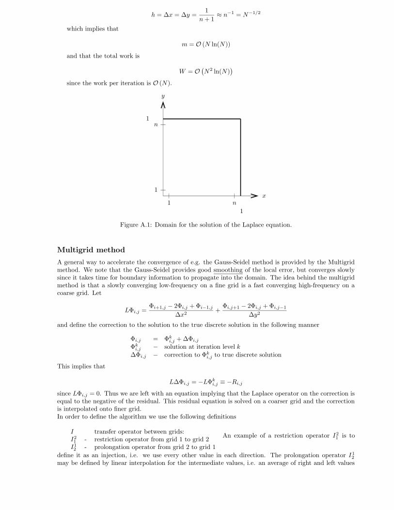
96 APPENDIX A. BACKGROUND MATERIAL
h = ∆x = ∆y =1
n+ 1≈ n−1 = N−1/2
which implies that
m = O (N ln(N))and that the total work is
W = O(N2 ln(N)
)
since the work per iteration is O (N).
PSfrag replacements
x, x1y, x2z, x3u, u1v, u2w, u3x1x2x 0i
ri(x 0i , t
)
ui(x 0i , t
)
P(t = 0
)
xu1
u2 > u1x1x2x3x 0i
ui dtdx 0
i
dui dtri(dt)
dri(dt)
P1
P2
x1x2x3R3
R2
R1
r3
r2
r1π2 + dϕ12
V (t)S (t)
V (t+∆t)− V (t)S (t+∆t)
un
V (t+∆t)
pT0, U0
TwLT0U0
Gradient fieldswi∂p∂xi
uiDivergence free vectorfields // to boundary
Lhx1x2
p0 > p1p1undS
u · n∆txyu0p0
η = y√4νtuu0
y = η√4νt
tηy
ωz =ω(η)·u0√
πνt
tLδ
ω ≈ 0U →y, vx, u
LUδu0
η = y√νx/u0
f ′ = uu0
Blasius profile
δ∗
xSeparation point
⇐= Pressure forcexy
luT
xy
dxdy
−dxdl = (dx, dy)
ndl = (dy,−dx)i− 1, j + 1
i, j + 1i+ 1, j + 1
cc′
bb′
i− 1, ji+ 1, j
i, jAabcd
dd′
aa′
i− 1, j − 1i, j − 1
i+ 1, j − 1j
ii+ 1ui,jvi,jpi,jpi,j
vi,j+1/2vi,j−1/2ui−1/2,ji− 1
2
ii+ 1
2
i+ 1i+ 3
2j + 1
2
jj − 1
2
j − 1ABC
u 32 ,1
v1, 32p1,1
012ij
InflowSolid wall
nΓ0Γ1Ω
M2
Mm
m+ 2
1hVVhuuhΓ0Γ1Ω
: to be updated
: new values: old values
i− 1i
i+ 1j − 1
jj + 1
iteration direction
x
y
1
1
1
1
n
n
Figure A.1: Domain for the solution of the Laplace equation.
Multigrid method
A general way to accelerate the convergence of e.g. the Gauss-Seidel method is provided by the Multigridmethod. We note that the Gauss-Seidel provides good smoothing of the local error, but converges slowlysince it takes time for boundary information to propagate into the domain. The idea behind the multigridmethod is that a slowly converging low-frequency on a fine grid is a fast converging high-frequency on acoarse grid. Let
LΦi,j =Φi+1,j − 2Φi,j +Φi−1,j
∆x2+Φi,j+1 − 2Φi,j +Φi,j−1
∆y2
and define the correction to the solution to the true discrete solution in the following manner
Φi,j = Φki,j +∆Φi,jΦki,j − solution at iteration level k∆Φi,j − correction to Φki,j to true discrete solution
This implies that
L∆Φi,j = −LΦki,j ≡ −Ri,jsince LΦi,j = 0. Thus we are left with an equation implying that the Laplace operator on the correction isequal to the negative of the residual. This residual equation is solved on a coarser grid and the correctionis interpolated onto finer grid.In order to define the algorithm we use the following definitions
I transfer operator between grids:I21 - restriction operator from grid 1 to grid 2I12 - prolongation operator from grid 2 to grid 1
An example of a restriction operator I21 is to
define it as an injection, i.e. we use every other value in each direction. The prolongation operator I12may be defined by linear interpolation for the intermediate values, i.e. an average of right and left values

A.2. CARTESIAN TENSOR NOTATION 97
PSfrag replacements
x, x1y, x2z, x3u, u1v, u2w, u3x1x2x 0i
ri(x 0i , t
)
ui(x 0i , t
)
P(t = 0
)
xu1
u2 > u1x1x2x3x 0i
ui dtdx 0
i
dui dtri(dt)
dri(dt)
P1
P2
x1x2x3R3
R2
R1
r3
r2
r1π2 + dϕ12
V (t)S (t)
V (t+∆t)− V (t)S (t+∆t)
un
V (t+∆t)
pT0, U0
TwLT0U0
Gradient fieldswi∂p∂xi
uiDivergence free vectorfields // to boundary
Lhx1x2
p0 > p1p1undS
u · n∆txyu0p0
η = y√4νtuu0
y = η√4νt
tηy
ωz =ω(η)·u0√
πνt
tLδ
ω ≈ 0U →y, vx, u
LUδu0
η = y√νx/u0
f ′ = uu0
Blasius profile
δ∗
xSeparation point
⇐= Pressure forcexy
luT
xy
dxdy
−dxdl = (dx, dy)
ndl = (dy,−dx)i− 1, j + 1
i, j + 1i+ 1, j + 1
cc′
bb′
i− 1, ji+ 1, j
i, jAabcd
dd′
aa′
i− 1, j − 1i, j − 1
i+ 1, j − 1j
ii+ 1ui,jvi,jpi,jpi,j
vi,j+1/2vi,j−1/2ui−1/2,ji− 1
2
ii+ 1
2
i+ 1i+ 3
2j + 1
2
jj − 1
2
j − 1ABC
u 32 ,1
v1, 32p1,1
012ij
InflowSolid wall
nΓ0Γ1Ω
M2
Mm
m+ 2
1hVVhuuhΓ0Γ1Ω
: to be updated
: new values: old values
i− 1i
i+ 1j − 1
jj + 1
iteration directionxy
1n
x
y
i
j
fine grid (1)
coarse grid (2)
Figure A.2: Two level grid.
and top and bottom values. The values marked with × in figure A.2 are then taken as an average of theaverages of the intermediate values.
Now we can define the following two level scheme:
1. LΦi,j iterated k times ⇒ LΦki,j = Ri,j
2. L∆Φi,j = −I21Ri,j iterated k times, ∆Φ0i,j = 0 (starting value) (here ∆Φi,j is definied on grid 2)
3. Φi,j = Φki,j + I
12∆Φi,j and goto 1.
at the end of 1. convergence is checked.Wesseling [10] estimated the work of the multigrid method to be W = O (N lnN), a substantial im-
provement over the Gauss-Seidel method.
A.2 Cartesian tensor notation
Tensor notation is a compact way to write vector and tensor formulas. Vectors and tensors are objectswhich are independent of the coordinate system they are represented in.In the Cartesian coordinate system in Figure A.3 we have the unit vectors
|ek| = 1 k = 1, 2, 3
The scalar product of two unit vectors is the Kronecker’s delta, δkl
ek · el = δkl =1 k = l0 k 6= l
and the position vector r is
r = x1e1 + x2e2 + x3e3 =
3∑
k=1
xkek = xkek.
The last expression make use of Einstein’s summation convention: when an index occurs twice in the sameexpression, the expression is implicitly summed over all values for that index.
Example
δkk = δll = δ11 + δ22 + δ33 = 3
δijaj = δi1a1 + δi2a2 + δi3a3 = ai.
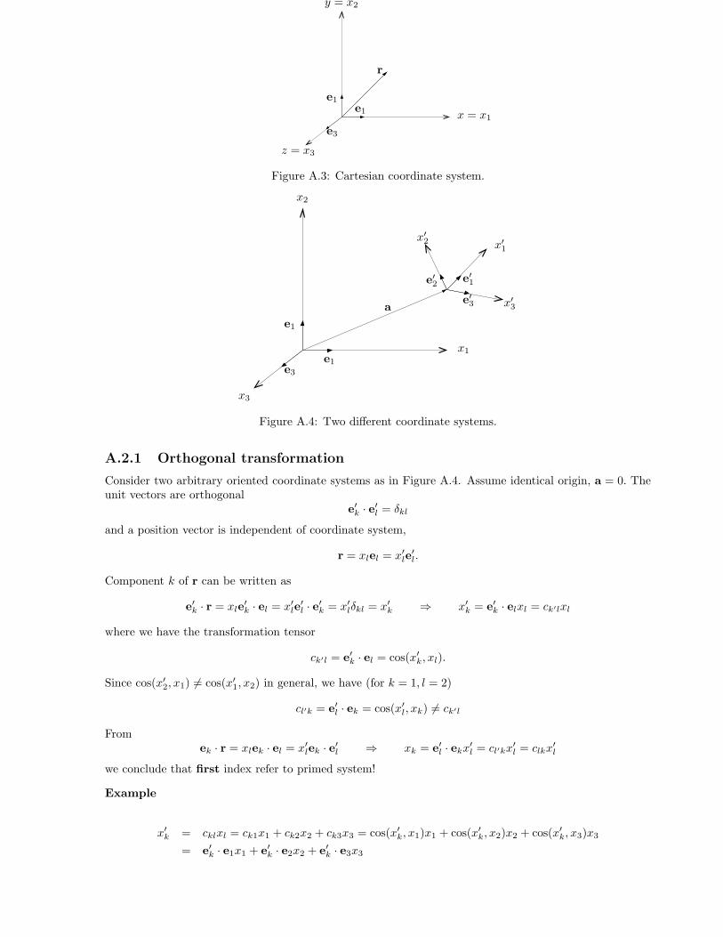
98 APPENDIX A. BACKGROUND MATERIAL
PSfrag replacements
x, x1y, x2z, x3u, u1v, u2w, u3x1x2x 0i
ri(x 0i , t
)
ui(x 0i , t
)
P(t = 0
)
xu1
u2 > u1x1x2x3x 0i
ui dtdx 0
i
dui dtri(dt)
dri(dt)
P1
P2
x1x2x3R3
R2
R1
r3
r2
r1π2 + dϕ12
V (t)S (t)
V (t+∆t)− V (t)S (t+∆t)
un
V (t+∆t)
pT0, U0
TwLT0U0
Gradient fieldswi∂p∂xi
uiDivergence free vectorfields // to boundary
Lhx1x2
p0 > p1p1undS
u · n∆txyu0p0
η = y√4νtuu0
y = η√4νt
tηy
ωz =ω(η)·u0√
πνt
tLδ
ω ≈ 0U →y, vx, u
LUδu0
η = y√νx/u0
f ′ = uu0
Blasius profile
δ∗
xSeparation point
⇐= Pressure forcexy
luT
xy
dxdy
−dxdl = (dx, dy)
ndl = (dy,−dx)i− 1, j + 1
i, j + 1i+ 1, j + 1
cc′
bb′
i− 1, ji+ 1, j
i, jAabcd
dd′
aa′
i− 1, j − 1i, j − 1
i+ 1, j − 1j
ii+ 1ui,jvi,jpi,jpi,j
vi,j+1/2vi,j−1/2ui−1/2,ji− 1
2
ii+ 1
2
i+ 1i+ 3
2j + 1
2
jj − 1
2
j − 1ABC
u 32 ,1
v1, 32p1,1
012ij
InflowSolid wall
nΓ0Γ1Ω
M2
Mm
m+ 2
1hVVhuuhΓ0Γ1Ω
: to be updated
: new values: old values
i− 1i
i+ 1j − 1
jj + 1
iteration directionxy
1nxy
ij
fine grid (1)coarse grid (2)
x = x1
y = x2
z = x3
r
e1e1
e2 e3
Figure A.3: Cartesian coordinate system.
PSfrag replacements
x, x1y, x2z, x3u, u1v, u2w, u3x1x2x 0i
ri(x 0i , t
)
ui(x 0i , t
)
P(t = 0
)
xu1
u2 > u1x1x2x3x 0i
ui dtdx 0
i
dui dtri(dt)
dri(dt)
P1
P2
x1x2x3R3
R2
R1
r3
r2
r1π2 + dϕ12
V (t)S (t)
V (t+∆t)− V (t)S (t+∆t)
un
V (t+∆t)
pT0, U0
TwLT0U0
Gradient fieldswi∂p∂xi
uiDivergence free vectorfields // to boundary
Lhx1x2
p0 > p1p1undS
u · n∆txyu0p0
η = y√4νtuu0
y = η√4νt
tηy
ωz =ω(η)·u0√
πνt
tLδ
ω ≈ 0U →y, vx, u
LUδu0
η = y√νx/u0
f ′ = uu0
Blasius profile
δ∗
xSeparation point
⇐= Pressure forcexy
luT
xy
dxdy
−dxdl = (dx, dy)
ndl = (dy,−dx)i− 1, j + 1
i, j + 1i+ 1, j + 1
cc′
bb′
i− 1, ji+ 1, j
i, jAabcd
dd′
aa′
i− 1, j − 1i, j − 1
i+ 1, j − 1j
ii+ 1ui,jvi,jpi,jpi,j
vi,j+1/2vi,j−1/2ui−1/2,ji− 1
2
ii+ 1
2
i+ 1i+ 3
2j + 1
2
jj − 1
2
j − 1ABC
u 32 ,1
v1, 32p1,1
012ij
InflowSolid wall
nΓ0Γ1Ω
M2
Mm
m+ 2
1hVVhuuhΓ0Γ1Ω
: to be updated
: new values: old values
i− 1i
i+ 1j − 1
jj + 1
iteration directionxy
1nxy
ij
fine grid (1)coarse grid (2)
x1
x2
x3
a
e1
e1
e2
e3
x′1x′2
x′3
e′1e′2
e′3
Figure A.4: Two different coordinate systems.
A.2.1 Orthogonal transformation
Consider two arbitrary oriented coordinate systems as in Figure A.4. Assume identical origin, a = 0. Theunit vectors are orthogonal
e′k · e′l = δkl
and a position vector is independent of coordinate system,
r = xlel = x′le′l.
Component k of r can be written as
e′k · r = xle′k · el = x′le
′l · e′k = x′lδkl = x′k ⇒ x′k = e′k · elxl = ck′lxl
where we have the transformation tensor
ck′l = e′k · el = cos(x′k, xl).
Since cos(x′2, x1) 6= cos(x′1, x2) in general, we have (for k = 1, l = 2)
cl′k = e′l · ek = cos(x′l, xk) 6= ck′l
Fromek · r = xlek · el = x′lek · e′l ⇒ xk = e′l · ekx′l = cl′kx
′l = clkx
′l
we conclude that first index refer to primed system!
Example
x′k = cklxl = ck1x1 + ck2x2 + ck3x3 = cos(x′k, x1)x1 + cos(x
′k, x2)x2 + cos(x
′k, x3)x3
= e′k · e1x1 + e′k · e2x2 + e′k · e3x3

A.2. CARTESIAN TENSOR NOTATION 99
PSfrag replacements
x, x1y, x2z, x3u, u1v, u2w, u3x1x2x 0i
ri(x 0i , t
)
ui(x 0i , t
)
P(t = 0
)
xu1
u2 > u1x1x2x3x 0i
ui dtdx 0
i
dui dtri(dt)
dri(dt)
P1
P2
x1x2x3R3
R2
R1
r3
r2
r1π2 + dϕ12
V (t)S (t)
V (t+∆t)− V (t)S (t+∆t)
un
V (t+∆t)
pT0, U0
TwLT0U0
Gradient fieldswi∂p∂xi
uiDivergence free vectorfields // to boundary
Lhx1x2
p0 > p1p1undS
u · n∆txyu0p0
η = y√4νtuu0
y = η√4νt
tηy
ωz =ω(η)·u0√
πνt
tLδ
ω ≈ 0U →y, vx, u
LUδu0
η = y√νx/u0
f ′ = uu0
Blasius profile
δ∗
xSeparation point
⇐= Pressure forcexy
luT
xy
dxdy
−dxdl = (dx, dy)
ndl = (dy,−dx)i− 1, j + 1
i, j + 1i+ 1, j + 1
cc′
bb′
i− 1, ji+ 1, j
i, jAabcd
dd′
aa′
i− 1, j − 1i, j − 1
i+ 1, j − 1j
ii+ 1ui,jvi,jpi,jpi,j
vi,j+1/2vi,j−1/2ui−1/2,ji− 1
2
ii+ 1
2
i+ 1i+ 3
2j + 1
2
jj − 1
2
j − 1ABC
u 32 ,1
v1, 32p1,1
012ij
InflowSolid wall
nΓ0Γ1Ω
M2
Mm
m+ 2
1hVVhuuhΓ0Γ1Ω
: to be updated
: new values: old values
i− 1i
i+ 1j − 1
jj + 1
iteration directionxy
1nxy
ij
fine grid (1)coarse grid (2)
e1x1
e1
e′2
e′2 · e1x1 = cos (x′2, x1)x1 = c21x1
Figure A.5: Projection of e1x1 on e′2.
which for component 2 reads
x′2 = e′2 · e1x1 + e′2 · e2x2 + e′2 · e3x3
∵ x′2 is projection of e1x1, e2x2, e3x3 on e′2. A visualization of the projection of e1x1 on e
′2 can be seen
in Figure A.5.
The relation between ckl and cml can be studied through
x′k︸︷︷︸
δkmx′m
= ckl xl︸︷︷︸
cmlx′m
= cklcmlx′m ⇒ (cklcml − δkm)x′m = 0.
In the same manner we have
xk︸︷︷︸
δkmxm
= clk x′l︸︷︷︸
clmxm
= clkclmxm ⇒ (clkclm − δkm)xm = 0.
A.2.2 Cartesian Tensors
Def. a Cartesian tensor of rank R is a set of quantities Tklm... which transform as a vector in each of itsR indices.
T ′klm... = ckrclscmp . . . Trsp...
ExampleFor scalars the rank is R = 0
a · b = a′k b′k = cklckm
︸ ︷︷ ︸
δlm
albm = albl,
for vectors R = 1
a′k = cklal
and for a tensor of second order we have R = 2
δ′kl = ckmclnδmn = ckmclm = δkl.
δkl is isotropic, i.e. identical in all coordinate systems.An outer product generates a tensor
T ′klS
′rs = ckmclncrpcsqTmnSpq
and an inner product generates a tensor
T ′klS
′ls = ckm clnclp
︸ ︷︷ ︸
δnp
csqTmnSpq = ckmcsqTmnSnq

100 APPENDIX A. BACKGROUND MATERIAL
A.2.3 Permutation tensor
εklm =
1−10
if klm is
evenoddno
permutation of (1, 2, 3)
As examples of permutations of 1,2,3 we have
(1,2,3), (3,1,2), (2,3,1) even permutation ε123 = 1(2,1,3), (3,2,1), (1,3,2) odd permutation ε213 = −1at least 2 subscripts equal no permutation ε221 = 0
A.2.4 Inner products, crossproducts and determinants
The inner product of the vectors a and b is
a · b = δijaibj = aibi = a1b1 + a2b2 + a3b3.
The cross product of a and b can be written as
a× b =
∣∣∣∣∣∣
e1 e2 e2a1 a2 a3b1 b2 b3
∣∣∣∣∣∣
= (a2b3 − a3b2)e1 + (a3b1 − a1b3)e2 + (a1b2 − a2b1)e3 = εijkeiajbk
and the determinant of the tensor aij is
|aij| =
∣∣∣∣∣∣
a11 a12 a13a21 a22 a23a31 a32 a33
∣∣∣∣∣∣
= εijka1ia2ja3k
=1
6εijk(ai1aj2ak3 + ai3aj1ak2 + ai2aj3ak1 − ai2aj1ak3 − ai3aj2ak1 − ai1aj3ak2 =
1
6εijkεpqraipajqakr.
We have the permutation relation
εklmεksp = δlsδmp − δlpδms. (A.1)
If we set s = l in (A.1) we getεklmεklp = (3− 1)δmp = 2δmp
and if we also use p = m we end up withεklmεklm = 6
The permutation tensor can also be used to derive the following vector relation
(a× b) · (c× d) = εijkajbkεilmcldm = (δjlδkm − δjmδlk)ajbkcldm= ajcjbkdk − ajdjbkck = (a · c)(b · d)− (a · d)(b · c)
A.2.5 Second rank tensors
All second rank tensors can be decomposed into symmetric and antisymmetric parts, Tkl = T(kl) + T[kl],where the antisymmetric part is
T[kl] = −T[lk] =1
2(Tkl − Tlk)
and the symmetric part
T(kl) = T(lk) =1
2(Tkl + Tlk) .
The symmetric part can be decomposed into isotropic and traceless part, T(kl) = T kl + T kl, the isotropicpart being
T kl =1
3Tmmδkl
and the traceless part is
T kl = T(kl) −1
3Tmmδkl.

A.2. CARTESIAN TENSOR NOTATION 101
If we project the isotropic, traceless and entisymmetric parts we get
S(kl)T[kl] =1
2
(S(kl)T[kl] + S(lk)T[lk]
)=1
2
(S(kl)T[kl] − S(lk)T[kl]
)= 0
SklT kl =1
3Smmδkl
(
T(kl) −1
3Tmmδkl
)
=1
3Smm
(
Tkk −1
3Tkkδll
)
= 0
⇒
SklT[kl] = S[kl]T[kl]
SklT(kl) = S(kl)T(kl)
SklT kl = SklT kl
SklT kl = SklT kl,
and each part is invariant under transformation
T ′[kl] = ckrclsT[rs] = −ckrclsT[sr] = −clrcksT[rs] = −T ′
[lk]
T ′rr = crpcrqTpq = δpqTpq = Tpp
T′kl = ckpclqT pq = ckpclq
(
T(pq) −1
3Trrδpq
)
= T ′(pq) −
1
3Trrδkl .
Since we only need three components to completely describe an antisymmetric tensor of rank R = 2 itcan be represented by its dual vector
di = εijkTjk =»»»»εijkT(jk) + εijkT[jk]
The first term on the right hand side is zero since εijk is antisymmetric in any two indecies. Multiply bothsides by εilm
εilmdi = εilmεijkTjk = (δljδmk − δlkδmj)Tjk = Tlm − Tml = 2T[lm] ⇒ T[lm] =1
2εilmdi
Note: There are 3 independent components in T[lm] and di.
In order to sum up, an arbitrary tensor of rank 2 can be divided into the following parts
Tkl = T(kl) + T[kl] = T kl + T kl + T[kl] =1
3Trrδkl︸ ︷︷ ︸
isotropic
+T(kl) −1
3Trrδkl
︸ ︷︷ ︸
traceless
+1
2εikldi︸ ︷︷ ︸
antisymmetric
Properties of the above parts are invariant under transformation. In the Navier-Stokes equations we havethe velocity gradient ∂ui
∂xj. The antisymmetric part of this tensor describes rotation, the isotropic part the
volume change and the traceless part describes the deformation of a fluid element.
ExampleWe have the second rank tensor
Tkl =
1 2 34 5 67 8 9
which can be divided into a symmetric part
T(kl)
=
1 3 53 5 75 7 9
and an antisymmetric part
T[kl]
=
0 −1 −21 0 −12 1 0
.
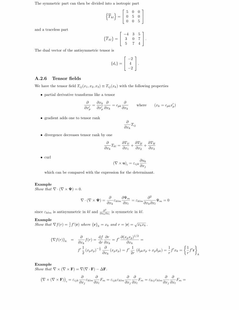
102 APPENDIX A. BACKGROUND MATERIAL
The symmetric part can then be divided into a isotropic part
T kl
=
5 0 00 5 00 0 5
and a traceless part
T kl=
−4 3 53 0 75 7 4
.
The dual vector of the antisymmetric tensor is
di =
−24−2
.
A.2.6 Tensor fields
We have the tensor field Tij(x1, x2, x3) ≡ Tij(xk) with the following properties
• partial derivative transforms like a tensor
∂
∂x′p=∂xk∂x′p
∂
∂xk= cpk
∂
∂xkwhere (xk = cpkx
′p)
• gradient adds one to tensor rank∂
∂xkTij
• divergence decreases tensor rank by one
∂
∂xkTkl =
∂T1l∂x1
+∂T2l∂x2
+∂T3l∂x3
• curl(∇× u)i = εijk
∂uk∂xj
which can be compared with the expression for the determinant.
ExampleShow that ∇ · (∇×Ψ) = 0.
∇ · (∇×Ψ) =∂
∂xkεklm
∂Ψm∂xl
= εklm∂2
∂xk∂xlΨm = 0
since εklm is antisymmetric in kl and ∂2
∂xk∂xlis symmetric in kl.
ExampleShow that ∇f(r) = 1
rf′(r) where rk = xk and r = |r| = √xkxk .
∇f(r)k =∂
∂xkf(r) =
df
dr
∂r
∂xk= f ′
∂(xpxp)1/2
∂xk=
f ′1
2(xpxp)
− 12 ∂
∂xk(xpxp) = f ′
1
2r(δpkxp + xpδpk) =
1
rf ′xk =
1
rf ′r
k
ExampleShow that ∇× (∇× F) = ∇(∇ · F)−∆F.(∇× (∇× F)
)
i= εijk
∂
∂xjεklm
∂
∂xlFm = εijkεklm
∂
∂xj
∂
∂xlFm = εkijεklm
∂
∂xj
∂
∂xlFm =

A.2. CARTESIAN TENSOR NOTATION 103
PSfrag replacements
x, x1y, x2z, x3u, u1v, u2w, u3x1x2x 0i
ri(x 0i , t
)
ui(x 0i , t
)
P(t = 0
)
xu1
u2 > u1x1x2x3x 0i
ui dtdx 0
i
dui dtri(dt)
dri(dt)
P1
P2
x1x2x3R3
R2
R1
r3
r2
r1π2 + dϕ12
V (t)S (t)
V (t+∆t)− V (t)S (t+∆t)
un
V (t+∆t)
pT0, U0
TwLT0U0
Gradient fieldswi∂p∂xi
uiDivergence free vectorfields // to boundary
Lhx1x2
p0 > p1p1undS
u · n∆txyu0p0
η = y√4νtuu0
y = η√4νt
tηy
ωz =ω(η)·u0√
πνt
tLδ
ω ≈ 0U →y, vx, u
LUδu0
η = y√νx/u0
f ′ = uu0
Blasius profile
δ∗
xSeparation point
⇐= Pressure forcexy
luT
xy
dxdy
−dxdl = (dx, dy)
ndl = (dy,−dx)i− 1, j + 1
i, j + 1i+ 1, j + 1
cc′
bb′
i− 1, ji+ 1, j
i, jAabcd
dd′
aa′
i− 1, j − 1i, j − 1
i+ 1, j − 1j
ii+ 1ui,jvi,jpi,jpi,j
vi,j+1/2vi,j−1/2ui−1/2,ji− 1
2
ii+ 1
2
i+ 1i+ 3
2j + 1
2
jj − 1
2
j − 1ABC
u 32 ,1
v1, 32p1,1
012ij
InflowSolid wall
nΓ0Γ1Ω
M2
Mm
m+ 2
1hVVhuuhΓ0Γ1Ω
: to be updated
: new values: old values
i− 1i
i+ 1j − 1
jj + 1
iteration directionxy
1nxy
ij
fine grid (1)coarse grid (2)
VS
n
dS = ndS
Figure A.6: Volume V bounded by the close surface S.
(δilδjm − δimδjl)∂
∂xj
∂
∂xlFm =
∂
∂xj
∂
∂xiFj −
∂
∂xj
∂
∂xjFi =
∂
∂xi
∂
∂xjFj −
∂
∂xj
∂
∂xjFi =
(∇(∇ · F)−∆F
)
i
Example
Show that if u = Ω× r then Ω =∇× u
2. This means, show that εijk
∂
∂xjuk = 2Ωi.
εijk∂
∂xjuk = uk = εklmΩlrm = εijk
∂
∂xj(εklmΩlrm) = εijkεklm
∂
∂xjΩlrm =
εkijεklm∂
∂xjΩlrm = (δilδjm − δimδjl)
∂
∂xjΩlrm =
∂
∂xmΩirm −
∂
∂xlΩlri = Ω independent of x = Ωi
∂rm∂xm
− Ωl∂ri∂xl
= ∂rm∂xm
= 1 + 1 + 1 = 3∂ri∂xl
= δil =
3Ωi − Ωlδil = 2Ωi
A.2.7 Gauss & Stokes integral theorems
Let n be the outward pointing normal to the closed surface S bounding the simply-connected volume V ,see Figure A.6. Gauss integral theorem then states
∮
S
a · ndS =∫
V
∇ · adV
or ∮
S
aknk dS =
∫
V
∂ak∂xk
dV
for a differentiable vector field a. This can be generalized to∮
S
Tklmnp dS =
∫
V
∂
∂xpTklm dV .
Example
∮
S
fndS =
∫
V
∇f dV .
∮
S
a× ndS =
∫
V
∇× adV if Tklmnm = εklmalnm.
Stokes theorem states that for a differentiable vector field a if an open simply-connected surface S isenclosed by a closed curve C, of which dl is the line element as in Figure A.7, then
∮
C
a · dl =∫
S
(∇× a) · ndS
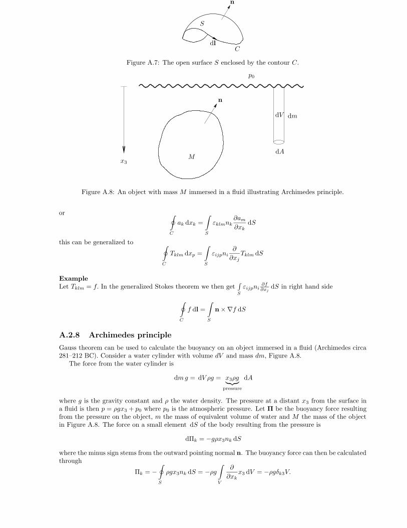
104 APPENDIX A. BACKGROUND MATERIAL
PSfrag replacements
x, x1y, x2z, x3u, u1v, u2w, u3x1x2x 0i
ri(x 0i , t
)
ui(x 0i , t
)
P(t = 0
)
xu1
u2 > u1x1x2x3x 0i
ui dtdx 0
i
dui dtri(dt)
dri(dt)
P1
P2
x1x2x3R3
R2
R1
r3
r2
r1π2 + dϕ12
V (t)S (t)
V (t+∆t)− V (t)S (t+∆t)
un
V (t+∆t)
pT0, U0
TwLT0U0
Gradient fieldswi∂p∂xi
uiDivergence free vectorfields // to boundary
Lhx1x2
p0 > p1p1undS
u · n∆txyu0p0
η = y√4νtuu0
y = η√4νt
tηy
ωz =ω(η)·u0√
πνt
tLδ
ω ≈ 0U →y, vx, u
LUδu0
η = y√νx/u0
f ′ = uu0
Blasius profile
δ∗
xSeparation point
⇐= Pressure forcexy
luT
xy
dxdy
−dxdl = (dx, dy)
ndl = (dy,−dx)i− 1, j + 1
i, j + 1i+ 1, j + 1
cc′
bb′
i− 1, ji+ 1, j
i, jAabcd
dd′
aa′
i− 1, j − 1i, j − 1
i+ 1, j − 1j
ii+ 1ui,jvi,jpi,jpi,j
vi,j+1/2vi,j−1/2ui−1/2,ji− 1
2
ii+ 1
2
i+ 1i+ 3
2j + 1
2
jj − 1
2
j − 1ABC
u 32 ,1
v1, 32p1,1
012ij
InflowSolid wall
nΓ0Γ1Ω
M2
Mm
m+ 2
1hVVhuuhΓ0Γ1Ω
: to be updated
: new values: old values
i− 1i
i+ 1j − 1
jj + 1
iteration directionxy
1nxy
ij
fine grid (1)coarse grid (2)
C
S
n
dl
Figure A.7: The open surface S enclosed by the contour C.
PSfrag replacements
x, x1y, x2z, x3u, u1v, u2w, u3x1x2x 0i
ri(x 0i , t
)
ui(x 0i , t
)
P(t = 0
)
xu1
u2 > u1x1x2x3x 0i
ui dtdx 0
i
dui dtri(dt)
dri(dt)
P1
P2
x1x2x3R3
R2
R1
r3
r2
r1π2 + dϕ12
V (t)S (t)
V (t+∆t)− V (t)S (t+∆t)
un
V (t+∆t)
pT0, U0
TwLT0U0
Gradient fieldswi∂p∂xi
uiDivergence free vectorfields // to boundary
Lhx1x2
p0 > p1p1undS
u · n∆txyu0p0
η = y√4νtuu0
y = η√4νt
tηy
ωz =ω(η)·u0√
πνt
tLδ
ω ≈ 0U →y, vx, u
LUδu0
η = y√νx/u0
f ′ = uu0
Blasius profile
δ∗
xSeparation point
⇐= Pressure forcexy
luT
xy
dxdy
−dxdl = (dx, dy)
ndl = (dy,−dx)i− 1, j + 1
i, j + 1i+ 1, j + 1
cc′
bb′
i− 1, ji+ 1, j
i, jAabcd
dd′
aa′
i− 1, j − 1i, j − 1
i+ 1, j − 1j
ii+ 1ui,jvi,jpi,jpi,j
vi,j+1/2vi,j−1/2ui−1/2,ji− 1
2
ii+ 1
2
i+ 1i+ 3
2j + 1
2
jj − 1
2
j − 1ABC
u 32 ,1
v1, 32p1,1
012ij
InflowSolid wall
nΓ0Γ1Ω
M2
Mm
m+ 2
1hVVhuuhΓ0Γ1Ω
: to be updated
: new values: old values
i− 1i
i+ 1j − 1
jj + 1
iteration directionxy
1nxy
ij
fine grid (1)coarse grid (2)
Mx3
n
dV dm
dA
p0
Figure A.8: An object with mass M immersed in a fluid illustrating Archimedes principle.
or ∮
C
ak dxk =
∫
S
εklmnk∂am∂xk
dS
this can be generalized to ∮
C
Tklm dxp =
∫
S
εijpni∂
∂xjTklm dS
ExampleLet Tklm = f. In the generalized Stokes theorem we then get
∫
S
εijpni∂f∂xj
dS in right hand side
∮
C
f dl =
∫
S
n×∇f dS
A.2.8 Archimedes principle
Gauss theorem can be used to calculate the buoyancy on an object immersed in a fluid (Archimedes circa281–212 BC). Consider a water cylinder with volume dV and mass dm, Figure A.8.
The force from the water cylinder is
dmg = dV ρg = x3ρg︸︷︷︸
pressure
dA
where g is the gravity constant and ρ the water density. The pressure at a distant x3 from the surface ina fluid is then p = ρgx3 + p0 where p0 is the atmospheric pressure. Let Π be the buoyancy force resultingfrom the pressure on the object, m the mass of equivalent volume of water and M the mass of the objectin Figure A.8. The force on a small element dS of the body resulting from the pressure is
dΠk = −gρx3nk dS
where the minus sign stems from the outward pointing normal n. The buoyancy force can then be calculatedthrough
Πk = −∮
S
ρgx3nk dS = −ρg∫
V
∂
∂xkx3 dV = −ρgδk3V.

A.2. CARTESIAN TENSOR NOTATION 105
PSfrag replacements
x, x1y, x2z, x3u, u1v, u2w, u3x1x2x 0i
ri(x 0i , t
)
ui(x 0i , t
)
P(t = 0
)
xu1
u2 > u1x1x2x3x 0i
ui dtdx 0
i
dui dtri(dt)
dri(dt)
P1
P2
x1x2x3R3
R2
R1
r3
r2
r1π2 + dϕ12
V (t)S (t)
V (t+∆t)− V (t)S (t+∆t)
un
V (t+∆t)
pT0, U0
TwLT0U0
Gradient fieldswi∂p∂xi
uiDivergence free vectorfields // to boundary
Lhx1x2
p0 > p1p1undS
u · n∆txyu0p0
η = y√4νtuu0
y = η√4νt
tηy
ωz =ω(η)·u0√
πνt
tLδ
ω ≈ 0U →y, vx, u
LUδu0
η = y√νx/u0
f ′ = uu0
Blasius profile
δ∗
xSeparation point
⇐= Pressure forcexy
luT
xy
dxdy
−dxdl = (dx, dy)
ndl = (dy,−dx)i− 1, j + 1
i, j + 1i+ 1, j + 1
cc′
bb′
i− 1, ji+ 1, j
i, jAabcd
dd′
aa′
i− 1, j − 1i, j − 1
i+ 1, j − 1j
ii+ 1ui,jvi,jpi,jpi,j
vi,j+1/2vi,j−1/2ui−1/2,ji− 1
2
ii+ 1
2
i+ 1i+ 3
2j + 1
2
jj − 1
2
j − 1ABC
u 32 ,1
v1, 32p1,1
012ij
InflowSolid wall
nΓ0Γ1Ω
M2
Mm
m+ 2
1hVVhuuhΓ0Γ1Ω
: to be updated
: new values: old values
i− 1i
i+ 1j − 1
jj + 1
iteration directionxy
1nxy
ij
fine grid (1)coarse grid (2)
Mg
mg
Figure A.9: The forces acting on an object immersed in a fluid. m is the mass of equivalent volume ofwater and M the mass of the body.
PSfrag replacements
x, x1y, x2z, x3u, u1v, u2w, u3x1x2x 0i
ri(x 0i , t
)
ui(x 0i , t
)
P(t = 0
)
xu1
u2 > u1x1x2x3x 0i
ui dtdx 0
i
dui dtri(dt)
dri(dt)
P1
P2
x1x2x3R3
R2
R1
r3
r2
r1π2 + dϕ12
V (t)S (t)
V (t+∆t)− V (t)S (t+∆t)
un
V (t+∆t)
pT0, U0
TwLT0U0
Gradient fieldswi∂p∂xi
uiDivergence free vectorfields // to boundary
Lhx1x2
p0 > p1p1undS
u · n∆txyu0p0
η = y√4νtuu0
y = η√4νt
tηy
ωz =ω(η)·u0√
πνt
tLδ
ω ≈ 0U →y, vx, u
LUδu0
η = y√νx/u0
f ′ = uu0
Blasius profile
δ∗
xSeparation point
⇐= Pressure forcexy
luT
xy
dxdy
−dxdl = (dx, dy)
ndl = (dy,−dx)i− 1, j + 1
i, j + 1i+ 1, j + 1
cc′
bb′
i− 1, ji+ 1, j
i, jAabcd
dd′
aa′
i− 1, j − 1i, j − 1
i+ 1, j − 1j
ii+ 1ui,jvi,jpi,jpi,j
vi,j+1/2vi,j−1/2ui−1/2,ji− 1
2
ii+ 1
2
i+ 1i+ 3
2j + 1
2
jj − 1
2
j − 1ABC
u 32 ,1
v1, 32p1,1
012ij
InflowSolid wall
nΓ0Γ1Ω
M2
Mm
m+ 2
1hVVhuuhΓ0Γ1Ω
: to be updated
: new values: old values
i− 1i
i+ 1j − 1
jj + 1
iteration directionxy
1nxy
ij
fine grid (1)coarse grid (2)
G
n
r− rG
Figure A.10: Moment around G from pressure forces acting on the object.
This means that the object loses some weight as the water is displaced. The buoyancy force is
Π3 = −ρgV = −gm
see Figure A.9.The moment of a force F at some arbitrary point with position vector r from the point of application of
the force isM = r×F. The moment around the center of gravity G of the homogenous body produced bythe pressure force dΠ acting on an element dS of the body is dMG = (r− rG)× dΠ as in Figure A.10.This can then be used to calculate the total moment around G form pressure forces on the body
MGk= −
∮
S
ρgεklm (xl − xGl)x3nm dS = −ρgεklm
∫
V
[∂
∂xm(xlx3)− xGl
∂x3∂xm
]
dV =
−ρgεklm∫
V
[δlmx3 + δm3xl − δm3xGl] dV = −ρgεkl3
∫
V
xl dV − xGlV
= 0
If a part of the fluid is frozen (without changing in density) this body is in equilibrium in the fluid:F =M = 0.

106 APPENDIX A. BACKGROUND MATERIAL
Appendix B
Supplementary material
B.1 Syllabus 2005
Computational Fluid Dynamics (5C1212), 5p.
Lecturers:
Dan Henningson (DH), [email protected], Mekanik, tel 790 9004
Katarina Gustavsson (KG), [email protected], NADA, tel 790 6696
Luca Brnadt (LB), [email protected], Mekanik, tel 790 7161
Erik Stalberg (ES), [email protected], Mekanik, tel 790 7161
Literature:
Copies from J.C. Tannehill, D.A. Anderson, R.H. Pletcher, Computational Fluid Mechanics and HeatTransfer, Taylor & Francis, 1997, (TAP)
Copies from Randall J LeVeque, Fininte Volume Method for Hyperbolic Problems, Cambridge UniversityPress, 2002 (LeV)
D. Henningson, Lecture notes on Computational Fluid Dynamics
K. Gustavsson, Lecture notes on Basic Numerics
Grading:
Test total of 50p., homeworks (required) 3×5 = 15p.Total points > 30 (3), > 40 (4), > 50 (5).
Web links
http://www.mech.kth.se/
Course plan
1. Tue 18/1 8-10, E51. Fluid dynamics I: LB
Introduction and outline of the course.
Derivation of the governing equations.
2. Wed 19/1 15-17, E51. Basic numerics I: KG
Mathematical behavior of hyperbolic, parabolic and elliptic equations. Well-posedness.KG Lecture notes
3. Thu 20/1 8-10, E35. Fluid dynamics II: LB
Derivation of the governing equations , cont.
107

108 APPENDIX B. SUPPLEMENTARY MATERIAL
4. Fri 21/1 15-17 L21. Basic numerics II: KG
Discretization by finite differences. Analysis of discretized equations; order of accuracy, convergenceand stability (von Neumann analysis).TAP: 3.1-3.3.5, 3.6, LeV: 8-8.2, 8.3.3
5. Tue 25/1 8-10, E51. Fluid dynamics III: LB
Derivation of the governing equations , cont.
6. Wed 26/1 15-17, Q36. Basic numerics III: KG
Numerical methods for model equations related to different levels of approximation of Navier Stokesequation: linear wave equation, Burgers equation, convection-diffusion equation. First and secondorder numerical methods such as upwind, Lax-Friedrichs, Lax-Wendroff, MacCormack, etc. Modifiedequation - dissipation and dispersion.TAP: 4.1-4.1.8, LeV: 8.6
7. Thu 27/1 8-10, V33. Fluid dynamics IV: LB
Dimensionless form, fluid phenomena, simplified equations
8. Fri 28/1 15-17, L21. Basic numerics IV: KG
Numerical methods for model equations, cont.
9. Mon 31/1 13-15, Q35. Compressible flow I: KG
Introduction to compressible flow. Euler equations, conservative/non-conservative form. Some ther-modynamics.LeV: 14
Scalar conservations laws: Conservation, weak solutions, non-uniqueness, entropy conditions. Shockformation, Rankine-Hugoniot relations.LeV: 11
10. Wed 2/2 15-17, E52. Compressible flow II: KG
Numerical methods for scalar conservation laws. Properties of the numerical scheme such as CFL-condition, conservation and TVD. First order methods. System of conservations lawsLeV: 4.1-4.9, 3
11. Fri 4/2 15-17, E52. Compressible flow III: KG
Numerical methods for Euler equations: MacCormack and artificial viscosity for non-linear systems.Numerical/physical boundary conditions. Shock tube problem.LeV: 3, 14
12. Tue 8/2 08-10, E51 . Compressible flow IV: KG
High resolution schemes for conservations laws.LeV: 6
13. Wed 9/2 15-17, D34. Compressible flow V: KG
Numerical methods for Euler equations. Boundary conditions, Riemann invariants. Compressibleflow in 2D.TAP: 6.3-6.7, LeV: 14
14. Fri 11/2 15-17, E35. Compressible flow VI: KG
Numerical methods for Euler equations, cont. Grids, algebraic mesh generation by transfinite inter-polation. Flow around an airfoil.
15. Tue 15/2 08-10, E3. Finite volume and finite difference methods I: DH
Laplace equation on arbitrary grids, equivalence with finite-differences, linear systems: Gauss-Seidelas smothers for multi-grid.
16. Wed 16/2 15-17, D34. Finite volume and finite difference methods II: DH
Introduction to incompressible flow. Properties of the equations, role of the pressure: artificialcompressibility and projection on divergence free space, Navier-Stokes in integral form.

B.2. STUDY QUESTIONS 109
17. Fri 18/2 15-17, E35. Finite volume and finite difference methods III: DH
Staggered grid/volume formulation + BC. Unsteady equations: projection and MAC method, dis-crete Poisson pressure eq.
18. Tue 22/2 8-10, Q34. Finite volume and finite difference methods IV: DH
Time step restrictions. Steady equations: distributive iteration and SIMPLE methods.
19. Thu 24/2 8-10, E35. Finite elements I: DH
An advection–diffusion problem. Variational form of the equation, weak solutions, essential andnatural boundary condition. Finite-element approximations, stability and accuracy, the algebraicproblem, matrix assembly.
20. Fri 25/2 15-17, E31. Finite elements II: DH
Navier–Stokes equations. Mixed variational form, Galerkin and FE approximations, the algebraicproblem. Stability, the LBB condition, mass conservation.
21. Tue 1/3 13-15, E31. Finite elements III: DH
Navier–Stokes equations. Mixed variational form, Galerkin and FE approximations, the algebraicproblem. Stability, the LBB condition, mass conservation.
22. Wed 2/3 15-17, Q33. Finite elements IV: DH
Navier–Stokes equations. Mixed variational form, Galerkin and FE approximations, the algebraicproblem. Stability, the LBB condition, mass conservation.
23. Sat 2/4 9-13, E31. EXAM.
Homeworks
• Homework 1A, due 31/1: Homework on NS equations.
• Homework 1B, due 31/1: Numerical methods for model equations. Different schemes. Dispersion,diffusion. Stability analysis.
• Homework 2, due 15/2: Numerical methods for non-linear conservation laws. Shock-tube.
• Homework 3, due 22/2: Running compressible Euler code; flow over a bump.
• Homework 4, due 1/3: FV homework + numerical project.
• Homework 5, due 8/3: FEM homework.
B.2 Study questions
1. Define and use the Rankine-Hugoniot jump condition to compute the shock speed for the followingproblem
ut + uux = 0 −∞ < x <∞, t > 0
u(x, 0) =
1 x ≤ 00 otherwise
2. Define the entropy condition for a scalar conservation law.
ut + f(u)x = 0 −∞ < x <∞, t > 0
with a convex flux function f(u). The shock is moving with speed s and the state to the left is givenby uL and the state to the right by uR.
Why do we need an entropy condition ?
3. Write a difference approximation (in 1D) on conservative form and define the notation.

110 APPENDIX B. SUPPLEMENTARY MATERIAL
4. Solve
ut + (u2
2)x = 0, u(x, 0) =
1 x < 0
0 x ≥ 0 (B.1)
by the upwind scheme on the following form,
un+1j = unj −∆t
∆xunj (u
nj − unj−1)
a) Will the numerical solution converge to the analytical solution?
b) If not, suggest another way of solving B.1.
5. Define a total variation decreasing (TVD) method. Why is this a desirable property ?
6. Investigate the one-sided difference scheme
un+1j = unj − a∆t
∆x(unj − unj−1)
for the advection equation
ut + aux = 0
Consider the cases a > 0 and a < 0.
a) Prove that the scheme is consistent and find the order of accuracy. Assume k/h constant.
b) Determine the stability requirement for a > 0 and show that it is unstable for a < 0.
7. Apply Lax-Friedrichs scheme to the linear wave equation
ut + aux = 0.
a) Write down the modified equation.
b) What type of equations is this?
c) What kind of behavior can we expect from the solution?
8. A the three-point centered scheme applied to
ut + aux = 0, a > 0.
yields the approximation
un+1j = unj +a∆t
2∆x(uj+1 − uj−1)
Show that this approximation is not stable even though the CFL condition is fulfilled.
9. What does Lax’s equivalence theorem state?
10. What is the condition on the n× n real matrix A(u) for the system
ut +Aux = 0
to be hyperbolic ?
11. The barotropic gas dynamic equations
ρt + ρux = 0 (B.2)
ut + uux +1
ρpx = 0
where
p = p(ρ) = Cργ
i and C a constant, can be linearized by considering small perturbations (ρ′, u′) around a motionlessgas.

B.2. STUDY QUESTIONS 111
gghhiijj kkll
mmnn
oooooooooo
ppppppppppn+1
PSfrag replacements
x, x1y, x2z, x3u, u1v, u2w, u3x1x2x 0i
ri(x 0i , t
)
ui(x 0i , t
)
P(t = 0
)
xu1
u2 > u1x1x2x3x 0i
ui dtdx 0
i
dui dtri(dt)
dri(dt)
P1
P2
x1x2x3R3
R2
R1
r3
r2
r1π2 + dϕ12
V (t)S (t)
V (t+∆t)− V (t)S (t+∆t)
un
V (t+∆t)
pT0, U0
TwLT0U0
Gradient fieldswi∂p∂xi
uiDivergence free vectorfields // to boundary
Lhx1x2
p0 > p1p1undS
u · n∆txyu0p0
η = y√4νtuu0
y = η√4νt
tηy
ωz =ω(η)·u0√
πνt
t
t
Lδ
ω ≈ 0U →y, vx, u
LUδu0
η = y√νx/u0
f ′ = uu0
Blasius profile
δ∗
xSeparation point
⇐= Pressure forcexy
luT
xy
dxdy
−dxdl = (dx, dy)
ndl = (dy,−dx)i− 1, j + 1
i, j + 1i+ 1, j + 1
cc′
bb′
i− 1, ji+ 1, j
i, jAabcd
dd′
aa′
i− 1, j − 1i, j − 1
i+ 1, j − 1j
ii+ 1ui,jvi,jpi,jpi,j
vi,j+1/2vi,j−1/2ui−1/2,ji− 1
2
ii+ 1
2
i+ 1i+ 3
2j + 1
2
jj − 1
2
j − 1ABC
u 32 ,1
v1, 32p1,1
012ij
InflowSolid wall
nΓ0Γ1Ω
M2
Mm
m+ 2
1hVVhuuhΓ0Γ1Ω
: to be updated
: new values: old values
i− 1i
i+ 1
j − 1
j
j + 1
iteration directionxy
1
n
xy
i
jfine grid (1)
coarse grid (2)
a) Let ρ = ρ0 + ρ′ and u = u0 + u′ where u0 = 0. Linearize the system (B.2) and show that thisyields the following linear system (the primes has been dropped)
ρt + ρ0ux = 0
ut +a2
ρ0ρx = 0 (B.3)
where a is the speed of sound. a and ρ0 are constants.
b) Is the system given by (B.3) a hyperbolic system? Motivate your answer.
c) Determine the characteristic variables in terms of ρ and u.
d) Determine the partial differential equations the characteristic variables fulfill - characteristic for-mulation.
e) Given initial conditions at t = 0 and let −∞ < x <∞ (no boundaries)
ρ(0, x) = sin(x) u(0, x) = 0
determine the analytical solution to (B.3) for t > 0. Hint: Start from the characteristic formulation.
12. The linearized form of (B.3) is given by
(ρu
)
t
+
(0 ρ0
a2/ρ0 0
)
︸ ︷︷ ︸
A
(ρu
)
x
= 0, (B.4)
where a is the speed of sound. a and ρ0 are constants.
a) Draw the domain of dependence of the solution to the system (B.4) in a point P in the x-t plane.
b) The system is solved numerically on a grid given by xj = j∆x, j = 0, 1, 2... and tn = n∆t, n =0, 1, 2, ..... using an explicit three-point scheme, see the figure below.
Draw the domain of dependence of the numerical solution at P (in the same figure as a)) of thethree-point scheme in the case when
i) the CFL condition is fulfilled
ii) the CFL condition is NOT fulfilled.
Assume that P is a grid point.
13. To solve Euler equations in 1D
ρt + ρux + uρx = 0
ut + uux +1
ρpx = 0
pt + ρc2ux + upx = 0
How many boundary conditions must be added at (motivate your answer)
inflow boundary when the flow is
a) Supersonic
b) Subsonic
outflow boundary when the flow is
c) Supersonic
d) Subsonic

112 APPENDIX B. SUPPLEMENTARY MATERIAL
14. Describe the ideas behind a flux splitting scheme for solving a non-linear hyperbolic system of equa-tions,
Ut + F (U)x = 0
15. a) Show that a vector field wi can be decomposed into
wi = ui +∂p
∂xi
where u is is divergence free and parallel to the boundary.
b) Apply this to the Navier-Stokes equations, show that the pressure term disappears and recover anequation for the pressure from the gradient part.
16. From the differential form of the Navier-Stokes equations obtain
a) the Navier-Stokes equations in integral form used in finite-volume discretizations,
b) a variational form of the Navier-Stokes equations used in finite-element discretizations.
17. a) Write down the appropriate function spaces for the pressure and velocity used to define weaksolutions to the Navier-Stokes equations.
b) Explain the concept of essential and natural boundary conditions.
18. a) How is a finite-element approximation defined?
b) Explain how to convert a FEM discretization to an algebraic problem, e.g. that the Navier-Stokesequations yield
(νK+C(u) G
GT 0
)(up
)
=
(f0
)
19. a) By choosing zh = uh in the finite element approximation of the Stokes problem, show that anyGalerkin velocity solution is stable.
b) Describe and interpret the LBB condition.
20. Choice of elements. Discrete elements pairs
a) constant pressure-bilinear velocities,
b) the Taylor-Hood pair,
c) a stable choice with piecewise linear velocities.
21. a) Derive the finite volume (FV) discretization on arbitrary grids of the continuity equation (∂ui/∂xi =0),
b) derive the FV discretization for Laplace equation on a Cartesian grid,
c) show that both are equivalent to a central difference approximation for Cartesian grids.
22. Derive the finite element (FEM) discretization for Laplace equation on a Cartesian grid and showthat it is equivalent to a central difference approximation.
23. Iterative techniques for linear systems.
a) Define Gauss-Seidel iterations for the Laplace equations,
b) Define the 2-level multigrid method for the Laplace equation,
24. State the difficulties associated with the the finite-volume discretizations of the Navier-Stokes equa-tions on a colocated grid? and show the form of the spurious solution which exist.
25. a) Define an appropriate staggered grid that can be used for the discretization of the Navier-Stokesequations,
b) write down the FV discretization of the Navier-Stokes equations on a staggered cartesian grid,
c) discuss how to treat noslip and inflow/outflow boundary conditions.
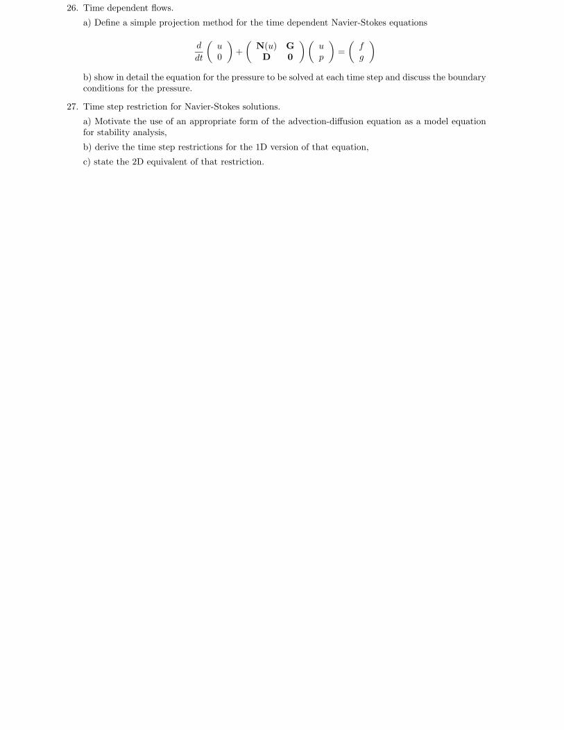
B.2. STUDY QUESTIONS 113
26. Time dependent flows.
a) Define a simple projection method for the time dependent Navier-Stokes equations
d
dt
(u0
)
+
(N(u) GD 0
)(up
)
=
(fg
)
b) show in detail the equation for the pressure to be solved at each time step and discuss the boundaryconditions for the pressure.
27. Time step restriction for Navier-Stokes solutions.
a) Motivate the use of an appropriate form of the advection-diffusion equation as a model equationfor stability analysis,
b) derive the time step restrictions for the 1D version of that equation,
c) state the 2D equivalent of that restriction.

114 APPENDIX B. SUPPLEMENTARY MATERIAL

Bibliography
[1] D.J. Acheson, 1990, Elementary Fluid Dynamics, Oxford University Press.
[2] J.D. Anderson, Jr., 1995, Computational Fluid Dynamics, The basics with applications, Mc Graw-Hill.
[3] C.A.J. Fletcher, 1991, Computational Techniques for Fluid Dynamics Volume 1, Second Edition,Springer-Verlag.
[4] C.A.J. Fletcher, 1991, Computational Techniques for Fluid Dynamics, Volume 2, Second Edition,Springer-Verlag.
[5] M. Griebel, T. Dornseifer and T. Neunhoeffer, 1998, Numerical Simulation in Fluid Dynamics, Apractical Introduction, SIAM Monographs on Mathematical Modeling and Computation.
[6] P.K. Kundu and I.M. Cohen, 2002, Fluid Mechanics, Second Edition, Academic Press.
[7] R.L. Panton, 1995, Incompressible Flow, Second Edition, Wiley-Interscience.
[8] R. Peyret, T.D. Taylor, 1983, Computational Methods for Fluid Flow, Springer-Verlag.
[9] J.C. Tannehill, D.A. Anderson and R.H. Pletcher, 1997, Computational Fluid Mechanics and HeatTransfer, Second Edition, Taylor and Francis.
[10] P. Wesseling, 2001, Principles of Computational Fluid Dynamics, Springer-Verlag.
115