Embed Size (px)
Citation preview

Lecture II: Continuous-Time and Discrete-Time
Signals
Maxim Raginsky
BME 171: Signals and Systems
Duke University
August 29, 2008
Maxim Raginsky Lecture II: Continuous-Time and Discrete-Time Signals
This lecture
Plan for the lecture:
1 Review: complex numbers
2 Continuous-time signals
unit step and unit rampunit impulsetransformations of time
3 Discrete-time signals
unit stepunit impulse
4 Periodic continuous-time and discrete-time signals
Maxim Raginsky Lecture II: Continuous-Time and Discrete-Time Signals

Review: complex numbers
Rectangular form: s = a + jb, j =√−1
a = Re(s), b = Im(s)
Polar form: s = rejθ
Euler’s formula: ejθ = cos θ + j sin θ
Complex conjugate: s∗ = a − jb = re−jθ
ss∗ = |s|2 = a2 + b2
0 Re s
Im s
θ
a
b
r = |s| =√
a2 + b2
θ = tan−1
(
b
a
)
Maxim Raginsky Lecture II: Continuous-Time and Discrete-Time Signals

Unit step and unit ramp
Unit step:
u(t) =
1, t ≥ 00, t < 0
u(t)
t0
1
Unit ramp:
r(t) =
t, t ≥ 00, t < 0 t0
1
1
r(t)
slop
e=1
Running integral representation:
r(t) =
∫ t
−∞
u(τ)dτ
Maxim Raginsky Lecture II: Continuous-Time and Discrete-Time Signals

Unit impulse
Unit impulse (aka Dirac delta-function):
1 δ(t) = 0 for t 6= 0
2∫ a
−aδ(t)dt = 1 for any a > 0
t0
(1)
δ(t)
The value of δ(t) at t = 0 is undefined; in particular, it is not +∞!
It is useful to think of δ(t) as an infinitesimally narrow pulse of unit areacentered around 0:
δ(t) = limε→0
δε(t),
where
δε(t) =
1/ε, −ε/2 ≤ t ≤ ε/20, |t| > ε/2
t
0
δε(t)
−ε/2 +ε/2
1/ε area=1
Maxim Raginsky Lecture II: Continuous-Time and Discrete-Time Signals
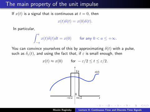
The main property of the unit impulse
If x(t) is a signal that is continuous at t = 0, then
x(t)δ(t) = x(0)δ(t).
In particular,∫ a
−a
x(t)δ(t)dt = x(0) for any 0 < a ≤ +∞.
You can convince yourselves of this by approximating δ(t) with a pulse,such as δε(t), and using the fact that, if ε is small enough, then
x(t) ≈ x(0) for − ε/2 ≤ t ≤ ε/2.
t
0−ε/2 +ε/2
1/ε x(t)
Maxim Raginsky Lecture II: Continuous-Time and Discrete-Time Signals
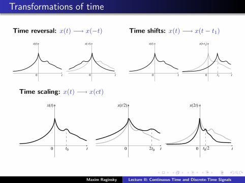
Transformations of time
Time reversal: x(t) −→ x(−t)
t0
x(t)
t0
x(-t)
Time shifts: x(t) −→ x(t − t1)
t0
x(t)
t0
x(t-t1)
t1
Time scaling: x(t) −→ x(ct)
t0
x(t)
t0
x(t/2)
t0
x(2t)
t0 2t0t0/2
Maxim Raginsky Lecture II: Continuous-Time and Discrete-Time Signals

Examples
Πτ (t) = u(
t + τ2
)
− u(
t − τ2
)
t0
Πτ(t)
-τ/2 τ/2
1
Λτ (t) = 2
τ
(
t + τ2
)
Πτ/2
(
t + τ4
)
− 2
τ
(
t − τ2
)
Πτ/2
(
t − τ4
)
t0
Λτ(t)
-τ/2 τ/2
1
Maxim Raginsky Lecture II: Continuous-Time and Discrete-Time Signals

More examples
x(t) = 2Π2.5(t − 0.25)
t0
x(t)
-1 1.5
2
x(t) = 2(t +2)Π1(t + 1.5)−2(t − 2)Π1(t − 1.5) + 2Π2(t)
t0
x(t)
-1 1
2
-2 2
x(t) =∑
∞
k=−∞g(t − kπ), where g(t) = tΠπ(t)
0
x(t)
-π π
1
−1
Maxim Raginsky Lecture II: Continuous-Time and Discrete-Time Signals
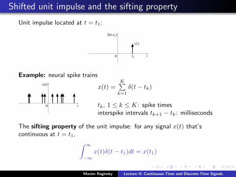
Shifted unit impulse and the sifting property
Unit impulse located at t = t1:
t0
(1)
δ(t-t1)
t1
Example: neural spike trains
t0
x(t)x(t) =
K∑
k=1
δ(t − tk)
tk, 1 ≤ k ≤ K: spike timesinterspike intervals tk+1 − tk: milliseconds
The sifting property of the unit impulse: for any signal x(t) that’scontinuous at t = t1,
∫
∞
−∞
x(t)δ(t − t1)dt = x(t1)
Maxim Raginsky Lecture II: Continuous-Time and Discrete-Time Signals
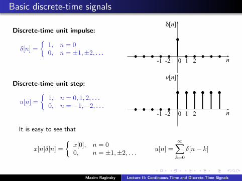
Basic discrete-time signals
Discrete-time unit impulse:
δ[n] =
1, n = 00, n = ±1,±2, . . .
0
δ[n]
n1 2-1 -2
Discrete-time unit step:
u[n] =
1, n = 0, 1, 2, . . .0, n = −1,−2, . . .
0
u[n]
n1 2-1 -2
It is easy to see that
x[n]δ[n] =
x[0], n = 00, n = ±1,±2, . . .
u[n] =
∞∑
k=0
δ[n − k]
Maxim Raginsky Lecture II: Continuous-Time and Discrete-Time Signals

Periodic continuous-time signals
x(t) is periodic if there exists a number T > 0, such that
x(t + T ) = x(t), for all t.
Fundamental period: smallest positive T , such that the above holds.
Examples:
0
x(t)
t
period = 2π/ω
sinusoid x(t) = A cos(ωt + θ)
0
x(t)
-π π
1
−1
period=π
triangular wave
Maxim Raginsky Lecture II: Continuous-Time and Discrete-Time Signals
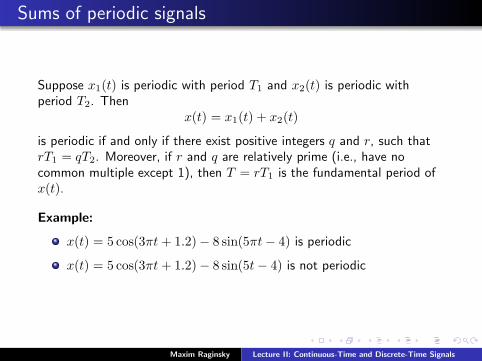
Sums of periodic signals
Suppose x1(t) is periodic with period T1 and x2(t) is periodic withperiod T2. Then
x(t) = x1(t) + x2(t)
is periodic if and only if there exist positive integers q and r, such thatrT1 = qT2. Moreover, if r and q are relatively prime (i.e., have nocommon multiple except 1), then T = rT1 is the fundamental period ofx(t).
Example:
x(t) = 5 cos(3πt + 1.2) − 8 sin(5πt − 4) is periodic
x(t) = 5 cos(3πt + 1.2) − 8 sin(5t − 4) is not periodic
Maxim Raginsky Lecture II: Continuous-Time and Discrete-Time Signals
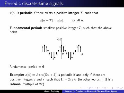
Periodic discrete-time signals
x[n] is periodic if there exists a positive integer T , such that
x[n + T ] = x[n], for all n.
Fundamental period: smallest positive integer T , such that the aboveholds.
x[n]
n0
fundamental period = 6
Example: x[n] = A cos(Ωn + θ) is periodic if and only if there are
positive integers q and r, such that Ω = 2πq/r (in other words, if Ω is a
rational multiple of 2π).
Maxim Raginsky Lecture II: Continuous-Time and Discrete-Time Signals