Lecture 5Continuous-time Queues (2)

Yin SunDept. Electrical and Computer Engineering

2

Outline� Continuous-time Markov Chains

� Little’s Law & M/M/1 Queue� Reading: Sections 9.2-9.3 of Srikant & Ying

� R. Srikant and Lei Ying, Communication Networks: An Optimization Control and Stochastic Networks Perspective, Cambridge University Press, 2014.

3

Continuous-time Queueing Systems

� Customers (or packets) arrive at a queue according to some arrival process, the service time of each customer is some random variable

� Arrival rate 𝜆: the average number of arriving customers per second

� Service rate 𝜇: the average number of customers served by a single server per second

4

Little’s Law

� Little’s Law also holds for continuous-time queues.� Little’s Law:

𝐿 = 𝜆 𝑊where 𝐿 is the average number of customers in the system, 𝑊 is the average time spent in the system, and 𝜆 is the arrival rate of the system.

5

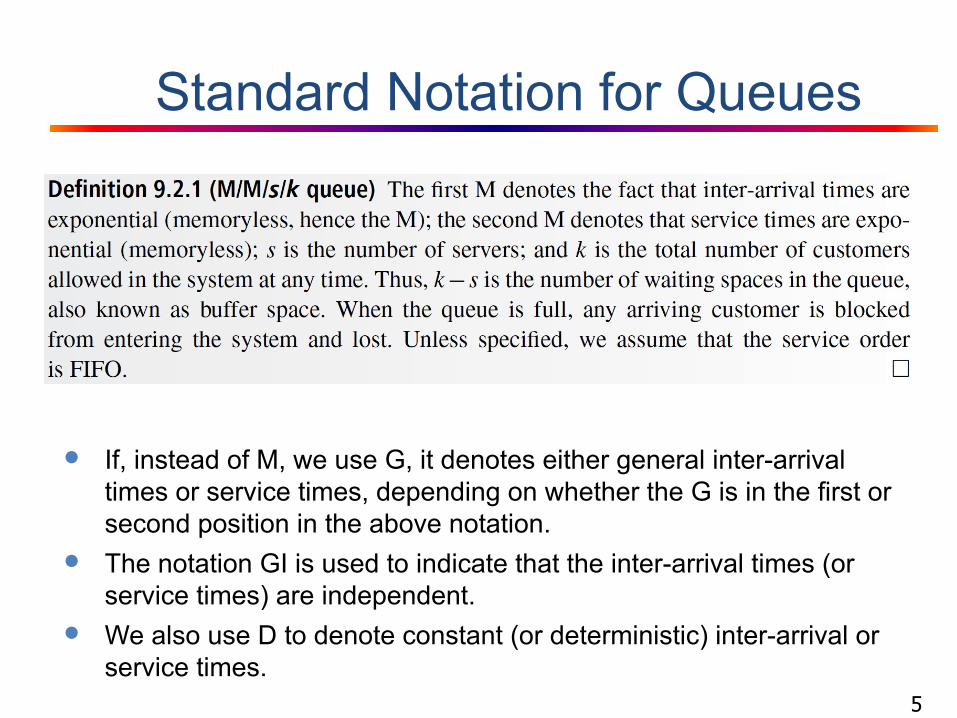
Standard Notation for Queues

� If, instead of M, we use G, it denotes either general inter-arrival times or service times, depending on whether the G is in the first or second position in the above notation.

� The notation GI is used to indicate that the inter-arrival times (or service times) are independent.

� We also use D to denote constant (or deterministic) inter-arrival or service times.

6

Poisson Process� An arrival process with exponentially distributed i.i.d. inter-

arrival times is called the Poisson process.

7

Poisson Process （2）

8

Uniformly Distributed Event Times� Let 𝑊!,𝑊", … ,𝑊# be the event times of a Poisson process.� Given 𝑋(𝑡) = 𝑛, the joint probability density function of 𝑊!,𝑊", … ,𝑊#

is given by

� If 𝑛 = 1, 𝑊! is uniformly distributed on [0, 𝑡].� If 𝑛 = 2, (𝑊!,𝑊") is uniformly distributed on a triangle shown below

𝑥!

𝑥"

𝑡

𝑡

9

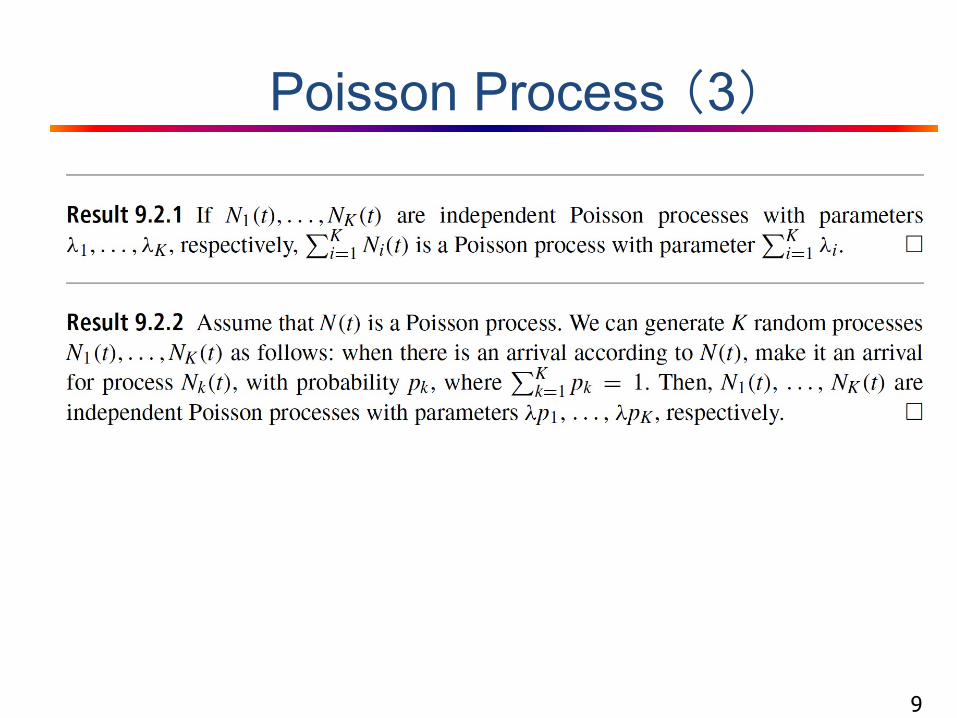
Poisson Process （3）

10

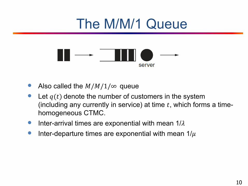
The M/M/1 Queue

� Also called the 𝑀/𝑀/1/∞ queue� Let 𝑞(𝑡) denote the number of customers in the system

(including any currently in service) at time 𝑡, which forms a time-homogeneous CTMC.

� Inter-arrival times are exponential with mean 1/𝜆� Inter-departure times are exponential with mean 1/𝜇

11

The M/M/1 Queue (2)

� Transition rate matrix 𝑸 is

� Derivations given in Srikant and Ying

12

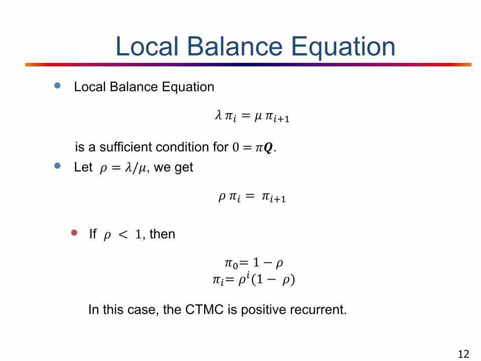
Local Balance Equation� Local Balance Equation

𝜆 𝜋$ = 𝜇 𝜋$%!

is a sufficient condition for 0 = 𝜋𝑸.� Let 𝜌 = 𝜆/𝜇, we get

𝜌 𝜋$ = 𝜋$%!

� If 𝜌 < 1, then

𝜋&= 1 − 𝜌𝜋$= 𝜌$(1 − 𝜌)

In this case, the CTMC is positive recurrent.

13

Performance of the M/M/1 Queue� The mean number of customers in the system:

𝐿 =;$'!

∞𝜌$(1 − 𝜌)𝑖 =

𝜌1 − 𝜌

� From Little’s law, the mean delay (i.e., waiting time in the queue + service time) of a customer:

𝑊= =>= ?

@ A >

� The mean waiting time of a customer in the queue:

𝑊( = 𝑊 −1𝜇=

𝜌𝜇 − 𝜆

14

Performance of the M/M/1 Queue (2)� The mean number of customers in the queue (again, by Little’s

law):

𝐿( = 𝜆𝑊( =𝜌"

1 − 𝜌

� Note that “the fraction of time the server is busy = Pr(there is at least one customer in the system)”� Hence, the fraction of time the server is busy is

𝑈 = 1 − 𝜋& = 𝜌

15

Performance of the M/M/1 Queue (3)� Note that “at most one customer can be in the server,” hence

𝐿) = average number of customers in the server= fraction of time that the server is busy = 𝑈 = 𝜌

� Waiting time in front of the server is

𝑊) = average amount of time spent by a customer in service= 1/𝜇.

� Applying Little’s law to the server alone, we obtain

𝑈 = 𝐿) = 𝜆𝑊) = 𝜆/𝜇 = 𝜌.

16

Summary� Little’s Law holds for continuous-time queues

� The M/M/1 queue � The mean queue length is 𝜌/(1 − 𝜌) and the mean delay is

1/(𝜇 − 𝜆).

� Reading: Sections 9.2-9.3 of Srikant & Ying