Lecture 6: Simple pricing review

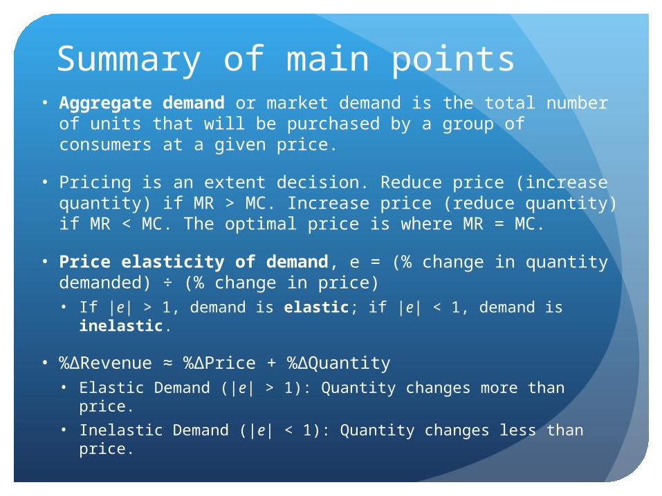
Summary of main points• Aggregate demand or market demand is the total number

of units that will be purchased by a group of consumers at a given price.

• Pricing is an extent decision. Reduce price (increase quantity) if MR > MC. Increase price (reduce quantity) if MR < MC. The optimal price is where MR = MC.

• Price elasticity of demand, e = (% change in quantity demanded) ÷ (% change in price)• If |e| > 1, demand is elastic; if |e| < 1, demand is inelastic.

• %ΔRevenue ≈ %ΔPrice + %ΔQuantity• Elastic Demand (|e| > 1): Quantity changes more than price.

• Inelastic Demand (|e| < 1): Quantity changes less than price.

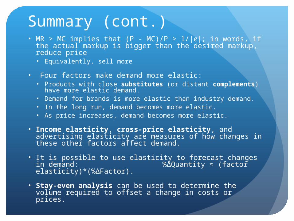
Summary (cont.)• MR > MC implies that (P - MC)/P > 1/|e|; in words, if the

actual markup is bigger than the desired markup, reduce price• Equivalently, sell more

• Four factors make demand more elastic:• Products with close substitutes (or distant complements)

have more elastic demand.• Demand for brands is more elastic than industry demand.• In the long run, demand becomes more elastic.• As price increases, demand becomes more elastic.

• Income elasticity, cross-price elasticity, and advertising elasticity are measures of how changes in these other factors affect demand.

• It is possible to use elasticity to forecast changes in demand: %ΔQuantity ≈ (factor elasticity)*(%ΔFactor).

• Stay-even analysis can be used to determine the volume required to offset a change in costs or prices.

KEY POINT #1

INDIVIDUAL DEMAND CURVES SLOPE DOWN…. THE LAW OF DEMAND!As we raise price, consumers will

respond by purchasing less.

4

Pricing trade-off• Pricing is an extent decision

• Profit= Total Revenue – Total Cost

• Demand curves turn pricing decisions into quantity decisions: “what price should I charge?” is equivalent to “how much should I sell?”

• Fundamental tradeoff:• Lower price sell more, but earn less on each unit

sold• Higher price sell less, but earn more on each unit

sold

• Tradeoff created by downward sloping demand

5

Pricing• Marginal analysis finds the profit increasing

solution to the pricing tradeoff.• It tells you only whether to raise or lower price, not

by how much.

• Definition: marginal revenue (MR) is change in total revenue from selling extra unit.

• If MR>0, then total revenue will increase if you sell one more. Highest level of MR doesn’t mean profits are maximized as we saw on our quiz.

• If MR>MC, then total profits will increase if you sell one more.

• We already know: Profits are maximized when MR = MC

6

KEY POINT #2

MARGINAL ANALYSIS TELLS US THAT WHEN MR>MC…. PRODUCE AND SELL MORE!!! HOW???? DECREASE PRICE

WHEN MR<MC…. WE ARE PRODUCING AND SELLING TOO MUCH…. SELL LESS!!! HOW??? INCREASE PRICE

7

Elasticity of demand

• Price elasticity is a factor in calculating MR.

• Definition: price elasticity of demand (e)• (% in Qd) (% in price)

• If |e| is less than one, demand is said to be inelastic.

• If |e| is greater than one, demand is said to be elastic.

8

Price change between month 1 and month 2

• Definition: Elasticity=

[(q2-q1)/(q1+q2)] [(p2-p1)/(p1+p2)].

• Note, by the law of demand, elasticity of price change should be negative.

• Example: On a promotion week for Vlasic, the price of Vlasic pickles dropped by 25% and quantity increased by 300%.• Is the price elasticity of demand -12?

• HINT: could something other than price be changing?

9

KEY POINT #3

WHEN DEMAND IS ELASTIC, RAISING THE PRICE WILL REDUCE REVENUE.

WHEN DEMAND IS INELASTIC, RAISING THE PRICE WILL RAISE REVENUE!!

Note: Remember revenue is only one side of the coin. We would need to know something about costs to determine if profit are maximized.

10

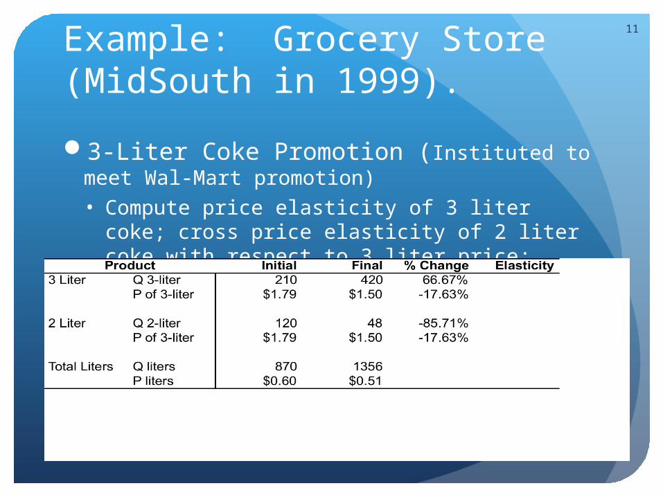
Example: Grocery Store (MidSouth in 1999).

3-Liter Coke Promotion (Instituted to meet Wal-Mart promotion)• Compute price elasticity of 3 liter coke; cross

price elasticity of 2 liter coke with respect to 3 liter price;

11

Revenue:

Demand for 3-liters was very elastic. Please calculate the revenue that resulted from the price decrease.

Did revenue increase or decrease?

Should increase as we already discussed.

We can show the %change in revenue is equal to the %change in price + % change in quantity.Since prices and quantities move in opposite

directions, total revenue changes will determined by which changes by more (in absolute value).

12

If you want, I’ll show you the math

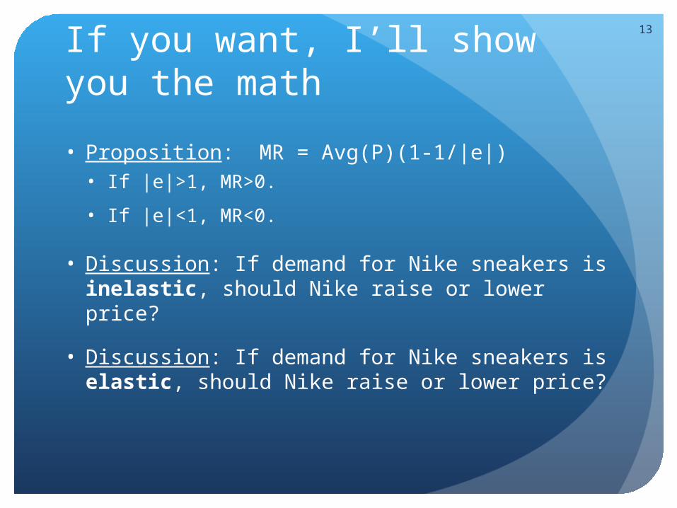
• Proposition: MR = Avg(P)(1-1/|e|)• If |e|>1, MR>0.

• If |e|<1, MR<0.

• Discussion: If demand for Nike sneakers is inelastic, should Nike raise or lower price?

• Discussion: If demand for Nike sneakers is elastic, should Nike raise or lower price?

13

Example

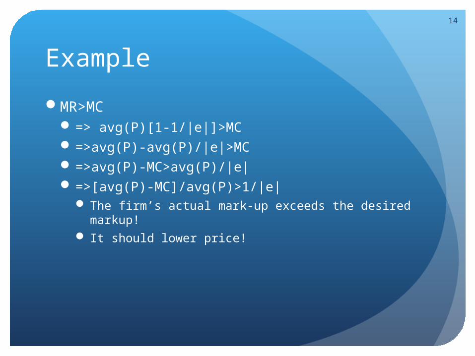
MR>MC=> avg(P)[1-1/|e|]>MC=>avg(P)-avg(P)/|e|>MC=>avg(P)-MC>avg(P)/|e|=>[avg(P)-MC]/avg(P)>1/|e|

The firm’s actual mark-up exceeds the desired markup! It should lower price!

14

Example

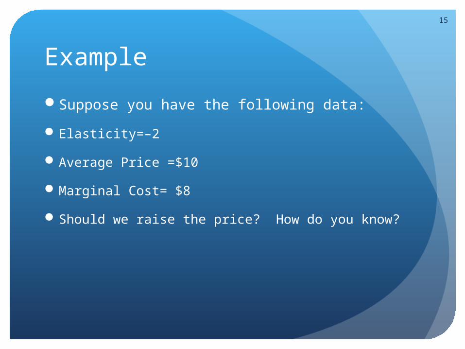
Suppose you have the following data:

Elasticity=–2

Average Price =$10

Marginal Cost= $8

Should we raise the price? How do you know?

15

Lecture 6: Topic #2Forecasting trend and

seasonality

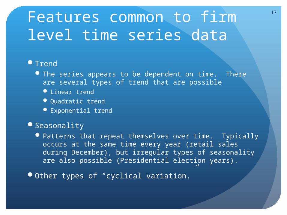
Features common to firm level time series data

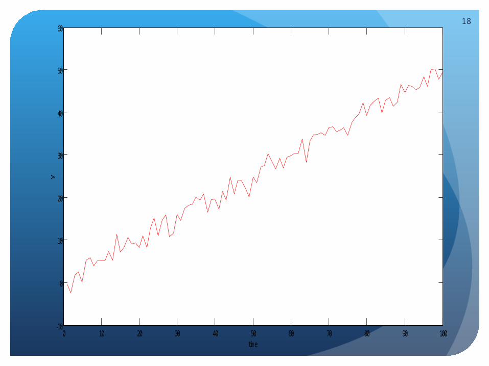
TrendThe series appears to be dependent on time. There are

several types of trend that are possible Linear trend Quadratic trend Exponential trend

SeasonalityPatterns that repeat themselves over time. Typically

occurs at the same time every year (retail sales during December), but irregular types of seasonality are also possible (Presidential election years).

Other types of “cyclical variation.”

17

18

0 10 20 30 40 50 60 70 80 90 100-10

0

10

20

30

40

50

60

time

y

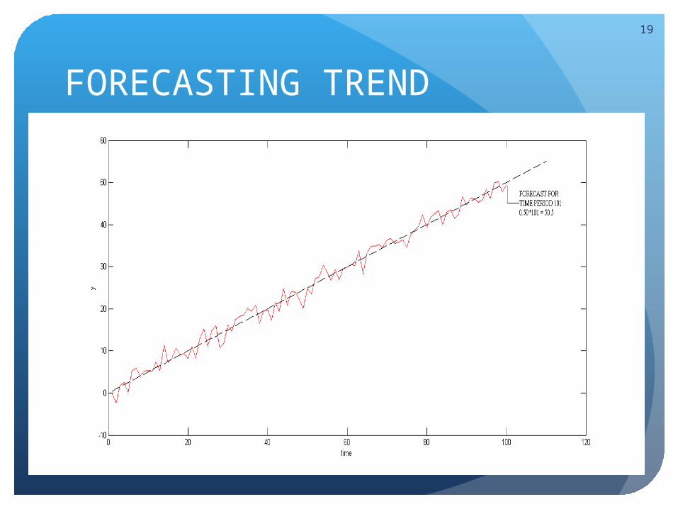
FORECASTING TREND

19

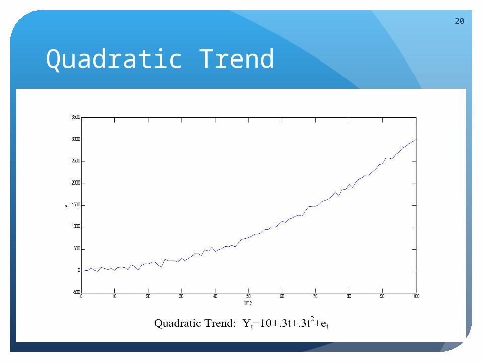
Quadratic Trend

20

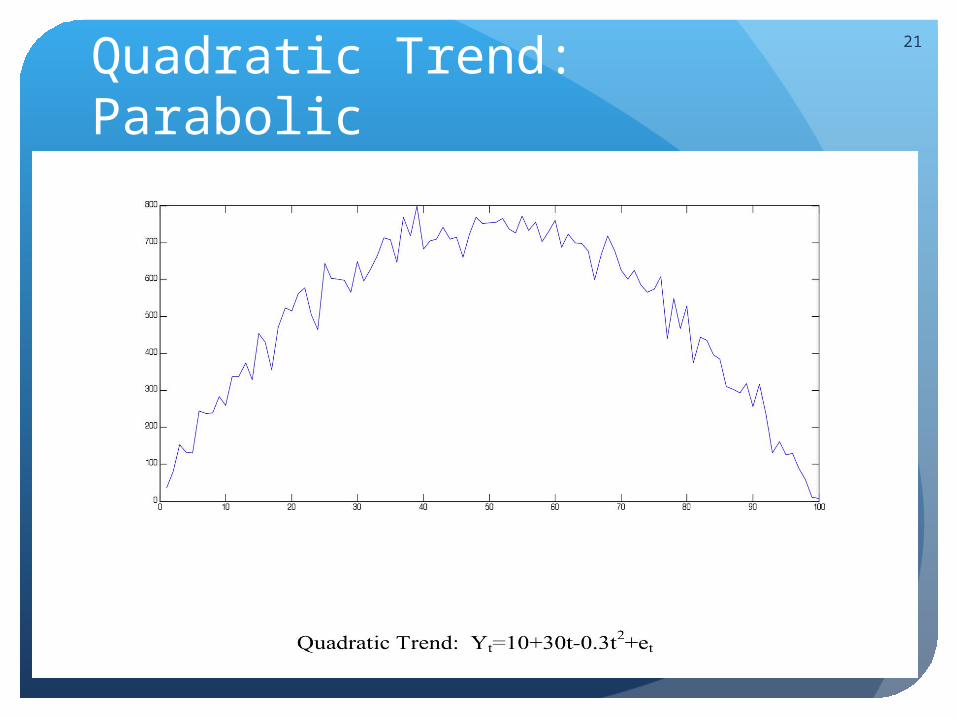
Quadratic Trend: Parabolic

21

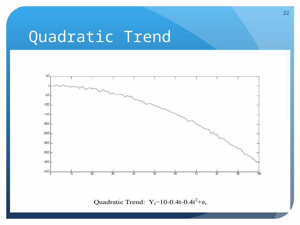
Quadratic Trend

22

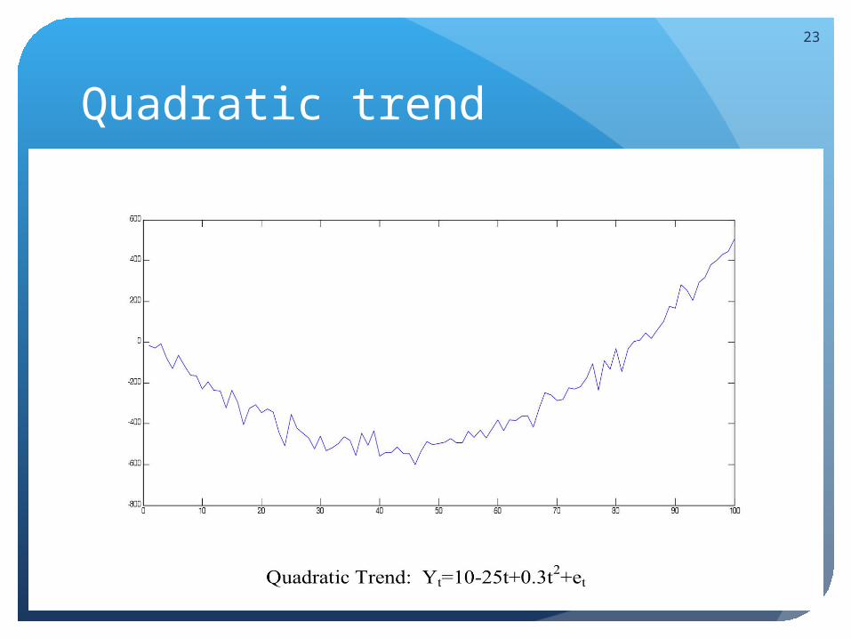
Quadratic trend

23

Modeling trend in EViews

Inspect the dataDoes the data appear to have a trend?

Is it linear? Is it quadratic? If the data appears to grow exponentially (population,

money supply, or perhaps even your firms sales) it may make sense to take the natural log of the variable. To do so in Eviews, we use the command “log.”

To create a linear time trend variable, suppose you call it ‘t’ use the following syntax in Eviews:genr t=@trend+1

24

Seasonality

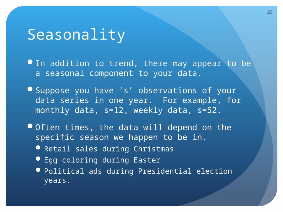
In addition to trend, there may appear to be a seasonal component to your data.

Suppose you have ‘s’ observations of your data series in one year. For example, for monthly data, s=12, weekly data, s=52.

Often times, the data will depend on the specific season we happen to be in.Retail sales during ChristmasEgg coloring during EasterPolitical ads during Presidential election years.

25

Modelling seasonality

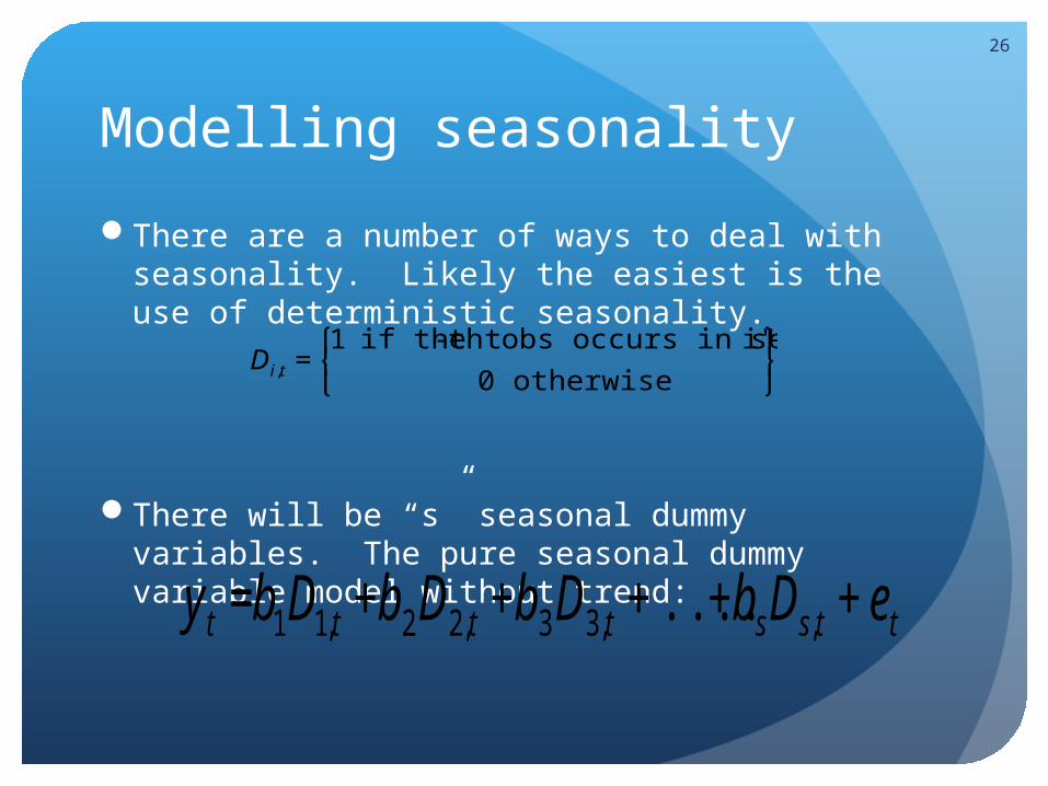
There are a number of ways to deal with seasonality. Likely the easiest is the use of deterministic seasonality.

There will be “s” seasonal dummy variables. The pure seasonal dummy variable model without trend:

26

€

Di,t =1 if the t - th obs occurs in season "i"

0 otherwise

⎧ ⎨ ⎩

⎫ ⎬ ⎭

€

y t =b1D1,t +b2D2,t +b3D3,t + ....+bsDs,t + et

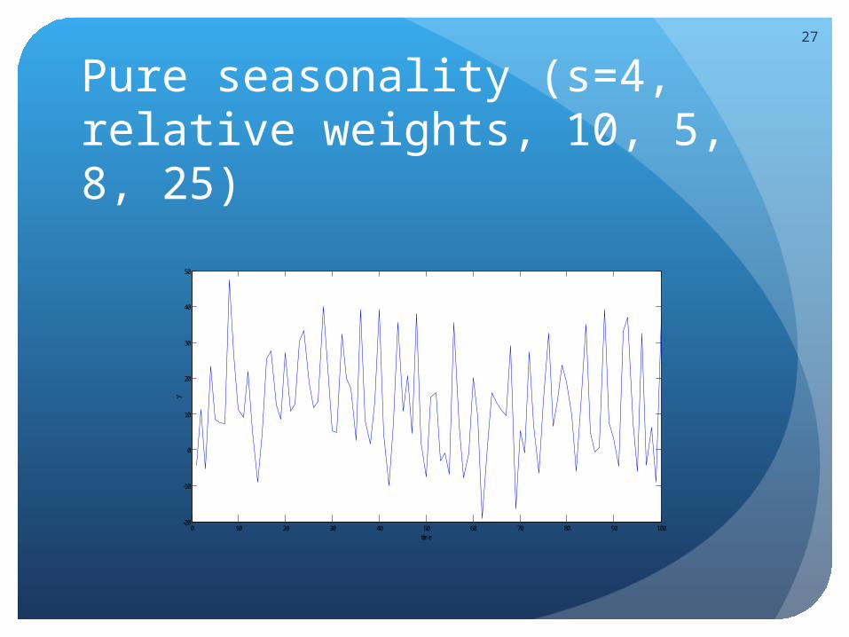
Pure seasonality (s=4, relative weights, 10, 5, 8, 25)

27

0 10 20 30 40 50 60 70 80 90 100-20

-10

0

10

20

30

40

50

time

y

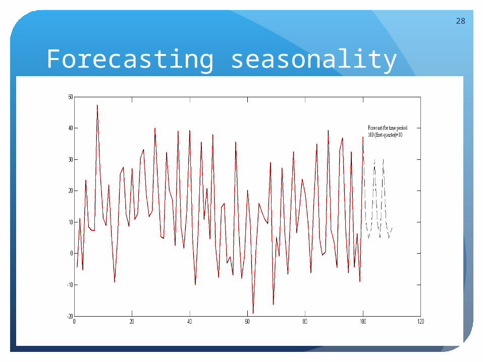
Forecasting seasonality

28

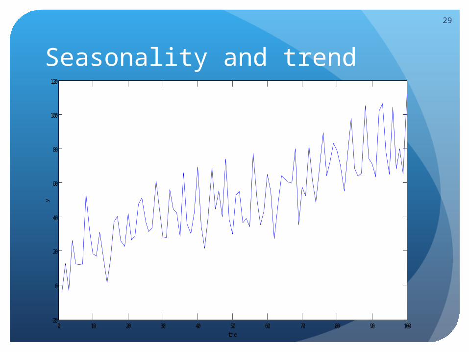
Seasonality and trend

29

0 10 20 30 40 50 60 70 80 90 100-20

0

20

40

60

80

100

120

time

y

To create seasonal dummies variables in Eviews, use the command “@seas().”

The first seasonal dummy variable is created:genr s1=@seas(1). IMPORTANT: If you include all “s” seasonal dummy

variable in your model, you must eliminate the constant from your regression model

30

Putting it all together

Often, seasonality and trend will account for a massive portion of the variance in the data. Even after accounting for these components, “something appears to be missing.”

In time series forecasting, the most powerful methods involve the use of ARMA components.

To determine if autoregressive-moving average components are present, we look at the correlogram of the residuals.

31

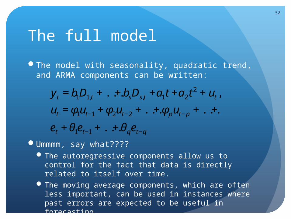
The full model

The model with seasonality, quadratic trend, and ARMA components can be written:

Ummmm, say what????The autoregressive components allow us to control

for the fact that data is directly related to itself over time.

The moving average components, which are often less important, can be used in instances where past errors are expected to be useful in forecasting.

32

€

y t = b1D1,t + ...+ bsDs,t +a1t +a2 t2 + ut ,

ut = φ1ut−1 + φ2ut−2 + ...+ φput− p + ...+

et +θ1et−1 + ...+θqet−q

Model selection

Autocorrelation (AC) can be used to choose a model. The autocorrelations measure any correlation or persistence. For ARMA(p,q) models, autocorrelations begin behaving like an AR(p) process after lag q.

Partial autocorrelations (PAC) only analyze direct correlations. For ARMA(p,q) processes, PACs begin behaving like an MA(q) process after lag p.

For AR(p) process, the autocorrelation is never theoretically zero, but PAC cuts off after lag p.

For MA(q) process, the PAC is never theoretically zero, but AC cuts off after lag q.

33

Model selection

An important statistic that can used in choosing a model is the Schwarz Bayesian Information Criteria. It rewards models that reduce the sum of squared errors, while penalizing models with too many regressors.SIC=log(SSE/T)+(k/T)log(T), where k is the number

of regressors.

The first part is our reward for reducing the sum of squared errors. The second part is our penalty for adding regressors. We prefer smaller numbers to larger number (-17 is smaller than -10).

34