LECTURE 6: Approximation by spline functions

October 29, 2012

1 First-degree and second-degree splines

1.1 First-degree spline

A spline function is a function that consists of polynomial pieces joined together withcertain smoothness conditions. For example, the polygonal function is a spline of degree1 which consists of linear polynomials joined together to achieve continuity. The pointst0, t1, . . . , tn are called knots.

S0 S1

S2S3

S7

S4

S5S6

a=t0 t1 t2 t3 t4 t5 t6 t7 t8=bx

In explicit form, the function must be defined piece by piece:

S(x) =

S0(x) x ∈ [t0, t1]S1(x) x ∈ [t1, t2]...Sn−1(x) x ∈ [tn−1, tn]

where each piece of S(x) is a linear polynomial:

Si(x) = aix+bi

A function such as S(x) is called piecewise linear.

1

Definition.A function S is called a spline of degree 1 if:

1. The domain of S is an interval [a,b].

2. S is continuous on [a,b].

3. There is a partitioning of the interval a = t0 < t1 < .. . < tn = b such that S is a linearpolynomial on each subinterval [ti, ti+1].

Example. The following function

S(x) =

x x ∈ [−1,0]1− x x ∈ (0,1)2x−2 x ∈ [1,2]

is not a spline because it is discontinuous at x = 0.

−1 −0.5 0 0.5 1 1.5 2

−1

−0.5

0

0.5

1

1.5

2

x

S(x)

Continuity of a function f at point s can be defined by the condition

limx→s+

f (x) = limx→s−

f (x) = f (s)

In other words, this means that the values of f must converge to the same limiting valuef (s) (which is the value of the function at s) from both above and below the point s.

2

Spline functions of degree 1 can be used for interpolation. Suppose that we have thefollowing table of values:

x t0 t1 . . . tny y0 y1 . . . yn

This can be represented by n+1 points in the xy-plane, and we can draw a polygonal line(a spline of degree 1) through the points.

The equation for the line segment on the interval [ti, ti+1] is given by

Si(x) = yi +mi(x− ti) = yi +yi+1− yi

ti+1− ti(x− ti)

Here mi is the slope of the line.

The following pseudocode is a function which utilizes n+ 1 table values to evaluate thefunction S(x):

real function Spline1(n, (ti), (yi), x)real array (ti)0:n,(yi)0:ninteger i,nreal xfor i=n-1 to 0 step -1 do

if x− ti ≤ 0 then exit loopend forSpline1 ← yi +(x− ti)[(yi+1− yi)/(ti+1− ti)]end function Spline1

3

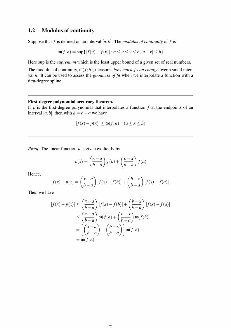
1.2 Modulus of continuity

Suppose that f is defined on an interval [a,b]. The modulus of continuity of f is

ω( f ;h) = sup{| f (u)− f (v)| : a≤ u≤ v≤ b, |u− v| ≤ h}

Here sup is the supremum which is the least upper bound of a given set of real numbers.

The modulus of continuity, ω( f ;h), measures how much f can change over a small inter-val h. It can be used to assess the goodness of fit when we interpolate a function with afirst-degree spline.

First-degree polynomial accuracy theorem.If p is the first-degree polynomial that interpolates a function f at the endpoints of aninterval [a,b], then with h = b−a we have

| f (x)− p(x)| ≤ ω( f ;h) (a≤ x≤ b)

Proof. The linear function p is given explicitly by

p(x) =(

x−ab−a

)f (b)+

(b− xb−a

)f (a)

Hence,

f (x)− p(x) =(

x−ab−a

)[ f (x)− f (b)]+

(b− xb−a

)[ f (x)− f (a)]

Then we have

| f (x)− p(x)| ≤(

x−ab−a

)| f (x)− f (b)|+

(b− xb−a

)| f (x)− f (a)|

≤(

x−ab−a

)ω( f ;h)+

(b− xb−a

)ω( f ;h)

=

[(x−ab−a

)+

(b− xb−a

)]ω( f ;h)

= ω( f ;h)

4

First-degree spline accuracy theorem.Let p be a first-degree spline having knots a = x0 < xi < .. . < xn = b. If p interpolates afunction f at these knots, then with h = max(xi− xi−1) we have

| f (x)− p(x)| ≤ ω( f ;h) (a≤ x≤ b)

This tells us that if more knots are inserted in such a way that the maximum spacing hgoes to zero, then the corresponding first-degree spline will converge uniformly to f .

Note that this type of a result does not exist in the polynomial interpolation theory! Thereincreasing the number of nodes may even lead to larger errors!

1.3 Second-degree splines

We are now considering piecewise quadratic functions, denoted by Q.

Definition.A function Q is called a spline of degree 2 if:

1. The domain of Q is an interval [a,b].

2. Q and Q′ are continuous on [a,b].

3. There are points ti (called knots) such that a = t0 < t1 < .. . < tn = b and Q is apolynomial of degree at most 2 on each subinterval [ti, ti+1].

In brief, a quadratic spline is a continuously differentiable piecewise quadratic function,where quadratic includes all linear combinations of the basic functions 1,x,x2.

5

Example. Consider the following function

Q(x) =

x2 x≤ 0−x2 0≤ x≤ 11−2x x≥ 1

The function is obviously piecewise quadratic. We can determine whether Q and Q′ arecontinuous by considering all the knot points separately:

limx→0−

Q(x) = limx→0−

x2 = 0 limx→0+

Q(x) = limx→0+

−x2 = 0

limx→1−

Q(x) = limx→1−

−x2 =−1 limx→1+

Q(x) = limx→1+

(1−2x) =−1

limx→0−

Q′(x) = limx→0−

2x = 0 limx→0+

Q′(x) = limx→0+

−2x = 0

limx→1−

Q′(x) = limx→1−

−2x =−2 limx→1+

Q′(x) = limx→1+

(−2) =−2

Thus, Q(x) is a quadratic spline.

−1 −0.5 0 0.5 1 1.5 2

−3

−2.5

−2

−1.5

−1

−0.5

0

0.5

1

x

Q(x)

6

1.4 Interpolating quadratic spline

Quadratic splines are not used in applications as often as natural cubic splines, but under-standing the simpler second-degree spline theory will help in grasping the more commonthird-degree splines.

Consider an interpolation problem with the following table of values:

x t0 t1 . . . tny y0 y1 . . . yn

Think of the nodes of the interpolation problem as being also the knots for the splinefunction to be constructed. A quadratic spline consists of n separate quadratic functions,Qi(x) = aix2 +bix+ ci. Thus we have 3n coefficients to determine.

The following conditions are imposed in order to determine the unknown coefficients:

(i) On each subinterval [ti, ti+1], the quadratic spline function Qi must satisfy the interpo-lation conditions: Qi(ti) = yi and Qi(ti+1) = yi+1. This imposes 2n conditions.

(ii) The continuity of Q does not impose any further conditions. But the continuity of Q′

at each of the interior points gives n−1 conditions.

(iii) We are now one condition short, since we have a total of 3n− 1 conditions from (i)and (ii). The last condition can be applied in different ways; e.g. Q′(t0) = 0 or Q′′0 = 0.

Derivation of the quadratic interpolating spline

We seek for a piecewise quadratic function

Q(x) =

Q0(x) x ∈ [t0, t1]Q1(x) x ∈ [t1, t2]...Qn−1(x) x ∈ [tn−1, tn]

which is continuously differentiable on the entire interval [t0, tn] and which interpolatesthe table:

Q(ti) = yi 0≤ i≤ n

Denote zi = Q′(ti). We can write the following formula for Qi:

Qi(x) =zi+1− zi

2(ti+1− ti)(x− ti)2 + zi(x− ti)+ yi

You can verify that: Qi(ti) = yi, Q′i(ti) = zi and Q′i(ti+1) = zi+1.

7

In order for Q to be continuous and to interpolate the data table, it is necessary and suffi-cient that Qi(ti+1) = yi+1 for i = 0,1, . . . ,n−1. This gives us the following:

zi+1 =−zi +2(

yi+1− yi

ti+1− ti

)(0≤ i≤ n−1)

This equation can be used to obtain the vector [z0,z1, . . . ,zn]T , starting with an arbitrary

value for z0 = Q′(t0).

Algorithm.(i.) Select z0 arbitrarily and compute z1, z2, . . . , zn using the recursion formula above.

(ii.) The quadratic spline interpolating function Q can now be constructed using the tablevalues for yi and ti together with the obtained values for zi.

2 Natural cubic splines

2.1 Splines of higher degree

First- and second-degree splines are not so useful for actual applications, because theirlow-order derivatives are discontinuous.

• For first-degree splines, the slope of the spline may change abruptly at the knots.

• For second-degree splines, the discontinuity is in the second derivative which meansthat the curvature of the quadratic spline changes abruptly at each node.

First-degree spline

−1 −0.5 0 0.5 1 1.5 2

0

0.5

1

1.5

2

x

S(x)

Second-degree spline

−1 −0.5 0 0.5 1 1.5 2

−3

−2.5

−2

−1.5

−1

−0.5

0

0.5

1

x

Q(x)

Higher-degree splines are useful whenever more smoothness is needed in the approximat-ing function.

8

Definition.A function S is called a spline of degree k if:

1. The domain of S is an interval [a,b].

2. S, S′, S′′, . . . ,S(k−1) are all continuous on [a,b].

3. There are points ti (the knots of S) such that a = t0 < t1 < .. . < tn = b and such thatS is a polynomial of degree at most k on each subinterval [ti, ti+1].

2.2 Natural cubic spline

Splines of degree 3 are called cubic splines. In this case, the spline function has twocontinuous derivatives which makes the graph of the function appear smooth.

We next turn to interpolating a table of given values using a cubic spline whose knotscoincide with the x values in the table.

x t0 t1 . . . tny y0 y1 . . . yn

The ti’s are the knots and are assumed to be arranged in ascending order. The function S,which we are constructing, consists of n cubic polynomial pieces:

S(x) =

S0(x) x ∈ [t0, t1]S1(x) x ∈ [t1, t2]...Sn−1(x) x ∈ [tn−1, tn]

Here Si denotes the cubic polynomial that will be used on the subinterval [ti, ti+1].

The interpolation conditions are

Si(ti) = yi (0≤ i≤ n)

The continuity conditions are imposed only at the interior knots t1, t2, . . . , tn−1:

limx→t−i

S(k)(ti) = limx→t+i

S(k)(ti) (k = 0,1,2)

Two extra conditions are needed in order to use all the degrees of freedom available. Wecan choose:

S′′(t0) = S′′(tn) = 0

The resulting spline function is termed a natural cubic spline.

9

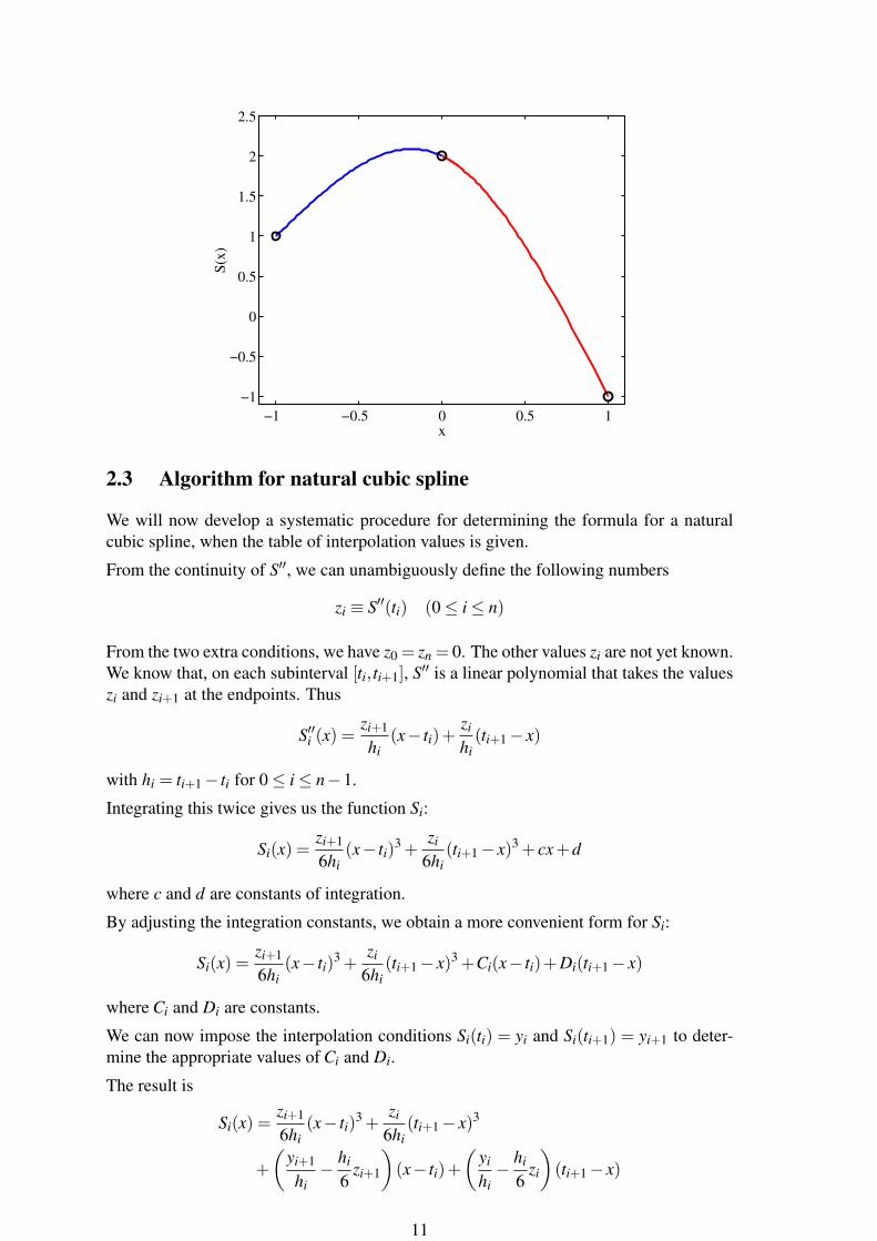
Example.

Determine the parameters a,b,c,d,e, f ,g and h so that S(x) is a natural cubic spline, where

S(x) =

{ax3 +bx2 + cx+d x ∈ [−1,0]ex3 + f x2 +gx+h x ∈ [0,1]

with interpolation conditions S(−1) = 1, S(0) = 2 and S(1) =−1.

Solution.

Let the two cubic polynomials be S0(x) and S1(x).

From the interpolation conditions we have

S0(0) = d = 2

S1(0) = h = 2

S0(−1) =−a+b− c =−1

S1(1) = e+ f +g =−3

The first derivative of S(x) is

S′(x) =

{3ax2 +2bx+ c3ex2 +2 f x+g

From the continuity condition of S′ we get

S′(0) = c = g

The second derivative is given by

S′′(x) =

{6ax+2b6ex+2 f

From the continuity of S′′ we get

S′′(0) = b = f

Two extra conditions areS′′(−1) =−6a+2b = 0

andS′′(1) =−6e+2 f = 0

From all these equations, we obtaina =−1, b =−3, c =−1, d = 2, e = 1, f =−3 and h = 2.

10

−1 −0.5 0 0.5 1

−1

−0.5

0

0.5

1

1.5

2

2.5

x

S(x)

2.3 Algorithm for natural cubic spline

We will now develop a systematic procedure for determining the formula for a naturalcubic spline, when the table of interpolation values is given.

From the continuity of S′′, we can unambiguously define the following numbers

zi ≡ S′′(ti) (0≤ i≤ n)

From the two extra conditions, we have z0 = zn = 0. The other values zi are not yet known.We know that, on each subinterval [ti, ti+1], S′′ is a linear polynomial that takes the valueszi and zi+1 at the endpoints. Thus

S′′i (x) =zi+1

hi(x− ti)+

zi

hi(ti+1− x)

with hi = ti+1− ti for 0≤ i≤ n−1.

Integrating this twice gives us the function Si:

Si(x) =zi+1

6hi(x− ti)3 +

zi

6hi(ti+1− x)3 + cx+d

where c and d are constants of integration.

By adjusting the integration constants, we obtain a more convenient form for Si:

Si(x) =zi+1

6hi(x− ti)3 +

zi

6hi(ti+1− x)3 +Ci(x− ti)+Di(ti+1− x)

where Ci and Di are constants.

We can now impose the interpolation conditions Si(ti) = yi and Si(ti+1) = yi+1 to deter-mine the appropriate values of Ci and Di.

The result is

Si(x) =zi+1

6hi(x− ti)3 +

zi

6hi(ti+1− x)3

+

(yi+1

hi− hi

6zi+1

)(x− ti)+

(yi

hi− hi

6zi

)(ti+1− x)

11

When the values z0,z1, . . . ,zn have been determined, the spline function S(x) is obtainedpiece by piece from this equation.

We now determine the zi’s. We use the remaining condition - namely the continuity of S′.At the interior knots ti for 1≤ i≤ n−1, we must have S′i−1(ti) = S′i(ti). We have

S′i(x) =zi+1

2hi(x− ti)2− zi

2hi(ti+1− x)2 +

yi+1

hi− hi

6zi+1−

yi

hi+

hi

6zi

This gives

S′i(ti) =−hi

6zi+1−

hi

3zi +bi,

wherebi =

1hi(yi+1− yi)

andhi = ti+1− ti.

Analogously, we have

S′i−1(ti) =−hi−1

6zi−1−

hi−1

3zi +bi−1

When these are set as equals, we get after rearrangement

hi−1zi−1 +2(hi−1 +hi)zi +hizi+1 = 6(bi−bi−1)

for 1≤ i≤ n−1.

By letting

ui = 2(hi−1 +hi)

vi = 6(bi−bi−1)

we obtain a tridiagonal system of equations:z0 = 0hi−1zi−1 +uizi +hizi+1 = vi (1≤ i≤ n−1)zn = 0

which is to be solved for the zi’s.

The first and last equations come from the natural cubic spline conditions S′′(t0)= S′′(tn)=0.

The tridiagonal system can be written in matrix form as follows:

1 0h0 u1 h1

h1 u2 h2. . . . . . . . .

0 1

z0z1z2...

zn−1zn

=

0v1v2...

vn−10

12

On eliminating the first and last equations, we obtainu1 h1h1 u2 h2

. . . . . . . . .hn−3 un−2 hn−2

hn−2 un−1

z1z2...

zn−2zn−1

=

v1v2...

vn−2vn−1

which is a symmetric tridiagonal system of order n−1.

Using the ideas presented in Chapter 5 of these lecture notes, we can develop an algorithmfor solving such a tridiagonal system.

The forward elimination phase in Gaussian elimination without pivoting would modifythe ui’s and vi’s as follows:ui← ui−

h2i−1

ui−1

vi← vi− hi−1vi−1ui−1

(i = 2,3, . . . ,n−1)

The back substitution yields{zn−i← vn−1

un−1

zi← vi−hizi+1ui

(i = n−2,n−3, . . . ,1)

13

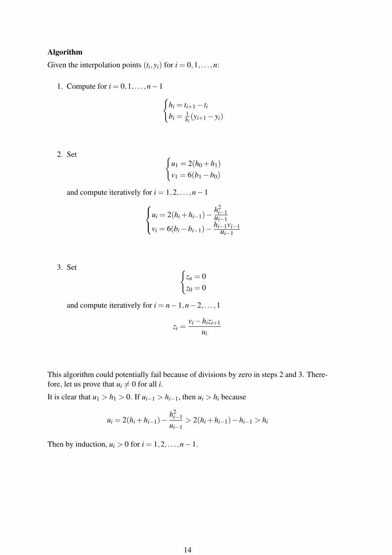
AlgorithmGiven the interpolation points (ti,yi) for i = 0,1, . . . ,n:

1. Compute for i = 0,1, . . . ,n−1{hi = ti+1− tibi =

1hi(yi+1− yi)

2. Set {u1 = 2(h0 +h1)

v1 = 6(b1−b0)

and compute iteratively for i = 1,2, . . . ,n−1ui = 2(hi +hi−1)−h2

i−1ui−1

vi = 6(bi−bi−1)− hi−1vi−1ui−1

3. Set {zn = 0z0 = 0

and compute iteratively for i = n−1,n−2, . . . ,1

zi =vi−hizi+1

ui

This algorithm could potentially fail because of divisions by zero in steps 2 and 3. There-fore, let us prove that ui 6= 0 for all i.

It is clear that u1 > h1 > 0. If ui−1 > hi−1, then ui > hi because

ui = 2(hi +hi−1)−h2

i−1

ui−1> 2(hi +hi−1)−hi−1 > hi

Then by induction, ui > 0 for i = 1,2, . . . ,n−1.

14

Evaluation of Si(x)

The following form for the cubic polynomial Si

Si(x) =zi+1

6hi(x− ti)3 +

zi

6hi(ti+1− x)3

+

(yi+1

hi− hi

6zi+1

)(x− ti)+

(yi

hi− hi

6zi

)(ti+1− x)

is not computationally very efficient.

A preferable form would be

Si(x) = Ai +Bi(x− ti)+Ci(x− ti)2 +Di(x− ti)3

Notice that the equation above is the Taylor expansion of Si about the point ti. Hence,

Ai = Si(ti) Bi = S′i(ti) Ci =12

S′′i (ti) Di =16

S′′′i (ti)

Therefore, Ai = yi and Ci = zi/2.

The coefficient of x3 is Di in the second form, whereas in the previously given form it is(zi+1− zi)/6hi. Thus

Di =1

6hi(zi+1− zi)

Finally, the value of S′i(ti) is given by

Bi =−hi

6zi+1−

hi

3zi +

1hi(yi+1− yi)

Thus the nested form of Si(x) is

Si(x) = yi +(x− ti)(

Bi +(x− ti)(

zi

2+

16hi

(x− ti)(zi+1− zi)

))

15

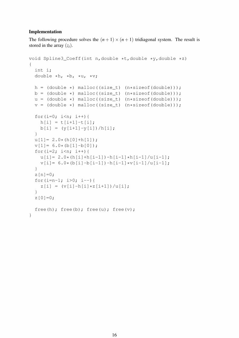
ImplementationThe following procedure solves the (n+ 1)× (n+ 1) tridiagonal system. The result isstored in the array (zi).

void Spline3_Coeff(int n,double *t,double *y,double *z){

int i;double *h, *b, *u, *v;

h = (double *) malloc((size_t) (n*sizeof(double)));b = (double *) malloc((size_t) (n*sizeof(double)));u = (double *) malloc((size_t) (n*sizeof(double)));v = (double *) malloc((size_t) (n*sizeof(double)));

for(i=0; i<n; i++){h[i] = t[i+1]-t[i];b[i] = (y[i+1]-y[i])/h[i];

}u[1]= 2.0*(h[0]+h[1]);v[1]= 6.0*(b[1]-b[0]);for(i=2; i<n; i++){

u[i]= 2.0*(h[i]+h[i-1])-h[i-1]*h[i-1]/u[i-1];v[i]= 6.0*(b[i]-b[i-1])-h[i-1]*v[i-1]/u[i-1];

}z[n]=0;for(i=n-1; i>0; i--){

z[i] = (v[i]-h[i]*z[i+1])/u[i];}z[0]=0;

free(h); free(b); free(u); free(v);}

16

The following procedure evaluates the natural cubic spline S(x) for a given value of x.The nested form is used in the evaluation of the Si’s.

double Spline3_Eval(int n, double *t,double *y, double *z, double x)

{int i;double h, tmp, result;

for(i=n-1; i>=0; i--) {if(x-t[i]>=0)

break;}h = t[i+1]-t[i];tmp = 0.5*z[i] + (x-t[i])*(z[i+1]-z[i])/(6.0*h);tmp = -(h/6.0)*(z[i+1]+2.0*z[i])+(y[i+1]-y[i])/h + (x-t[i])*tmp;result = y[i] + (x-t[i])*tmp;

return(result);}

17

Example

As an example, the natural cubic spline routines were implemented in a program whichdetermines the natural cubic spline interpolant for sinx at ten equidistant knots in theinterval [0,1.6875]. The spline function is evaluated at 37 equally spaced points in thesame interval. The figure below shows the spline function and the ten equidistant knots.

0 0.5 1 1.5

0

0.2

0.4

0.6

0.8

1knotsspline

The figure below shows the error |S(x)−sin(x)|, and for comparison, also the error |p(x)−sin(x)| obtained for the Newton form of the interpolating polynomial (Chapter 3). We notethat in this case the spline interpolant is not as accurate as the polynomial!

0 0.5 1 1.5

0

2

4

6

8

10

12

14

16

x 10−4

x

erro

r

splinepolynomial

18

Example 2

Here is another example which illustrates the differences between polynomial interpola-tion and cubic spline interpolation. Consider the serpentine curve given by

y =x

1/4+ x2

In order to have non-uniformly spaced knots, we write the curve in parametric form:{x = 1

2 tanθ

y = sin2θ

and take θ = i(π/12), where i =−5, . . . ,5.

If we use the parametric representation to generate the knots {x(θ),y(θ)}, the order of theknots must be rearranged so that the array (ti) runs from the smallest value to the largest.The values in array (yi) are also rearranged to correspond to the ordering of (ti). Afterthis, we can use the procedures Spline3_Coeff and Spline3_Eval to determinethe cubic spline interpolant of the serpentine curve.

The figure below shows the 13 knots, the polynomial interpolant and the cubic spline in-terpolant of the serpentine curve. Notice how the polynomial becomes wildly oscillatory,whereas the spline is an excellent fit.

−2 −1 0 1 2−6

−4

−2

0

2

4

6knotspolynomialspline

19

2.4 Smoothness property

The previous example illustrates why spline functions are better for data fitting than or-dinary polynomials. Interpolation by high-degree polynomials is often unsatisfactory be-cause polynomials exhibit oscillations.

Wild oscillations in a function can be attributed to its derivatives being very large. Forexample, for the curve in the figure below, f ′(x) is first large and positive and soon afterlarge and negative. Consequently, there is a point where f ′′(x) is large (since the value off ′ changes rapidly).

1 1.2 1.4 1.6 1.8 2 2.2

0

500

1000

1500

f’(x) < 0 f’(x) > 0

Spline functions do not exhibit such oscillatory behavior. In fact, from a certain point ofview, spline functions are the optimal functions for curve fitting.

Cubic spline smoothness theorem.If S is the natural cubic spline function that interpolates a twice-continuously differen-tiable function f at knots a = t0 < t1 < .. . < tn = b, then∫ b

a[S′′(x)]2dx≤

∫ b

a[ f ′′(x)]2dx

This theorem states that the average value of [S′′(x)]2 on the interval [a,b] is never largerthan the average value of [ f ′′(x)]2 on the same interval. Since [ f ′′(x)]2 is related to the cur-vature of f , we know that the spline interpolant will not oscillate more than the functionf itself does.

20

3 B splines

B splines are special spline functions that are well suited for numerical tasks. B splinesare often used in software packages for approximating data, and therefore, familiaritywith these functions is useful for anyone using such library codes. The name of B splinescomes from the fact that they form a basis for the set of all splines.

Here we assume that an infinite set of knots {ti} has been prescribed in such a way that{. . . < t−2 < t−1 < t0 < t1 < t2 < .. .

limi→∞ ti = ∞ =− limi→∞ t−i

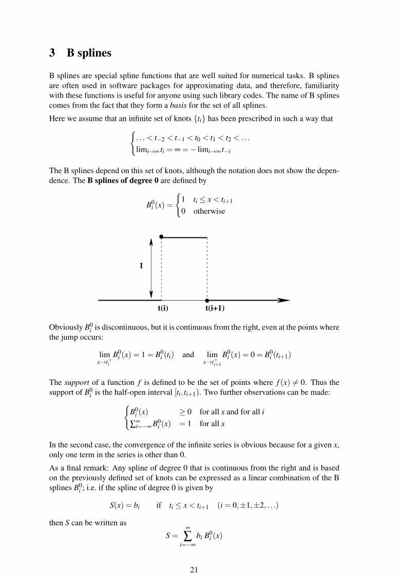
The B splines depend on this set of knots, although the notation does not show the depen-dence. The B splines of degree 0 are defined by

B0i (x) =

{1 ti ≤ x < ti+1

0 otherwise

t(i+1)t(i)

1

Obviously B0i is discontinuous, but it is continuous from the right, even at the points where

the jump occurs:

limx→t+i

B0i (x) = 1 = B0

i (ti) and limx→t+i+1

B0i (x) = 0 = B0

i (ti+1)

The support of a function f is defined to be the set of points where f (x) 6= 0. Thus thesupport of B0

i is the half-open interval [ti, ti+1). Two further observations can be made:{B0

i (x) ≥ 0 for all x and for all i

∑∞i=−∞ B0

i (x) = 1 for all x

In the second case, the convergence of the infinite series is obvious because for a given x,only one term in the series is other than 0.

As a final remark: Any spline of degree 0 that is continuous from the right and is basedon the previously defined set of knots can be expressed as a linear combination of the Bsplines B0

i ; i.e. if the spline of degree 0 is given by

S(x) = bi if ti ≤ x < ti+1 (i = 0,±1,±2, . . .)

then S can be written as

S =∞

∑i=−∞

bi B0i (x)

21

Higher degree splines

Using the functions B0i as a starting point, we can generate all the higher degree splines

by a simple recursive definition:

Bki (x) =

(x− ti

ti+k− ti

)Bk−1

i (x)+(

ti+k+1− xti+k+1− ti+1

)Bk−1

i+1 (x) (∗)

where k = 1,2, . . . and i = 0,±1,±2, . . ..

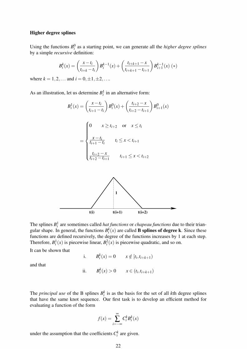
As an illustration, let us determine B1i in an alternative form:

B1i (x) =

(x− ti

ti+1− ti

)B0

i (x)+(

ti+2− xti+2− ti+1

)B0

i+1(x)

=

0 x≥ ti+2 or x≤ ti

x− titi+1− ti ti ≤ x < ti+1

ti+2− xti+2− ti+1

ti+1 ≤ x < ti+2

t(i+1)t(i) t(i+2)

1

The splines B1i are sometimes called hat functions or chapeau functions due to their trian-

gular shape. In general, the functions Bki (x) are called B splines of degree k. Since these

functions are defined recursively, the degree of the functions increases by 1 at each step.Therefore, B1

i (x) is piecewise linear, B2i (x) is piecewise quadratic, and so on.

It can be shown thati. Bk

i (x) = 0 x /∈ [ti, ti+k+1)

and thatii. Bk

i (x)> 0 x ∈ (ti, ti+k+1)

The principal use of the B splines Bki is as the basis for the set of all kth degree splines

that have the same knot sequence. Our first task is to develop an efficient method forevaluating a function of the form

f (x) =∞

∑i=−∞

Cki Bk

i (x)

under the assumption that the coefficients Cki are given.

22

Using the recursive definition of Bki (x), we obtain

f (x) =∞

∑i=−∞

Cki

[(x− ti

ti+k− ti

)Bk−1

i (x)+(

ti+k+1− xti+k+1− ti+1

)Bk−1

i+1 (x)]

=∞

∑i=−∞

[Ck

i

(x− ti

ti+k− ti

)+Ck

i−1

(ti+k− xti+k− ti

)]Bk−1

i (x)

=∞

∑i=−∞

Ck−1i Bk−1

i (x)

where Ck−1i is defined to be the appropriate coefficient from the second line of the equation

above.

This algebraic manipulation shows how a linear combination of Bki (x) can be expressed

as a linear combination of Bk−1i (x). Repeating the process k−1 times, gives

f (x) =∞

∑i=−∞

C0i B0

i (x)

The formula by which the coefficients C j−1i are obtained is

C j−1i =C j

i

(x− ti

ti+ j− ti

)+C j

i−1

(ti+ j− xti+ j− ti

)Now, in order to calculate f (x) on the interval tm ≤ x < tm+1 we only need k+ 1 coeffi-cients since

f (x) =∞

∑i=−∞

Cki Bk

i (x) =m

∑i=m−k

Cki Bk

i (x)

The coefficients Ckm,C

km−1, . . . ,C

km−k can be calculated from the equation (*) by forming

the following triangular array:

Ckm Ck−1

m . . . . . . C0m

Ckm−1 Ck−1

m−1 . . . C1m−1

... . . .

Ckm−k

We can now establish that

f (x) =∞

∑i=−∞

Bki (x) = 1 for all x and all k ≥ 0

We already know this for k = 0. For k > 0, we set Cki = 1 for all i. We can show (by

induction) that all the subsequent coefficients Cki ,C

k−1i , . . . ,C0

i are also equal to 1. Thus,at the end,

f (x) =∞

∑i=−∞

C0i B0

i (x) =∞

∑i=−∞

B0i (x) = 1

Therefore the sum of all B splines of degree k is unity.

23

Differentiation and integration

In many applications, B splines can be used as substitutes for complex functions. Differ-entiation and integration are important examples.

The smoothness of B splines Bki increases with the index k. It can be shown that Bk

i has acontinuous (k−1)th derivative. A basic result about the derivatives of B splines is

ddx

Bki (x) =

(k

ti+k− ti

)Bk−1

i (x)−(

kti+k+1− ti+1

)Bk−1

i+1 (x)

This can be proven by induction using the recursive formula (*). Using this result, we getthe following useful formula

ddx

∞

∑i=−∞

ciBki (x) =

∞

∑i=−∞

diBk−1i (x)

where

di = k(

ci− ci−1

ti+k− ti

)

B splines are also recommended for numerical integration. Here is a basic result:∫ x

−∞

Bki (s)ds =

(ti+k+1− ti+1

k+1

)∞

∑j=1

Bk+1j (x)

This can be verified by differentiating both sides with respect to x.

This leads to the following useful formula∫ x

−∞

∞

∑i=−∞

ciBki (s)ds =

∞

∑i=−∞

eiBk+1i (x)

where

ei =1

k+1

i

∑j=−∞

c j(t j+k+1− t j)

This formula gives an indefinite integral of any function expressed as a linear combinationof B splines. Any definite integral can be obtained by selecting a specific value for x.

For example, if x is a knot, say x = tm, then∫ tm

−∞

∞

∑i=−∞

ciBki (s)ds =

∞

∑i=−∞

eiBk+1i (tm) =

m

∑i=m−k−1

eiBk+1i (tm)

Matlab has a Spline toolbox which can be used for many tasks involving splines. Forexample, there are routines for interpolating data by splines and routines for least-squaresfits to data. There are also many demonstrations. Use the Matlab help command to learnmore about the properties.

24

4 Interpolation and approximation by B splines

We will now concentrate on the task of obtaining a B-spline representation of a givenfunction. We begin by considering the problem of interpolating a set of data. Later anoninterpolatory method of approximation is discussed.

A basic question is how to determine the coefficients in the expression

S(x) =∞

∑i=−∞

AiBki−k(x)

so that the resulting spline function interpolates a prescribed table of data:

x t0 t1 . . . tny y0 y1 . . . yn

Interpolation means thatS(ti) = yi (0≤ i≤ n)

B splines of degree 0We begin with the simplest splines, corresponding to k = 0:

B0i (t j) = δi j =

{1 i = j0 i 6= j

Here the solution is obvious: we set Ai = yi for 0 ≤ i ≤ n. All other coefficients arearbitrary.

Thus the zero-degree B spline

S(x) =n

∑i=0

yiB0i (x)

has the required interpolation property.

B splines of degree 1The next case, k = 1, also has a simple solution. The first-degree spline B1

i (x) can bedefined recursively using B0

i (x):

B1i (x) =

(x− ti

ti+1− ti

)B0

i (x)+(

ti+2− xti+2− ti+1

)B0

i+1(x)

=

0 x≥ ti+2 or x≤ ti

x− titi+1− ti ti < x < ti+1

ti+2− xti+2− ti+1

ti+1 ≤ x < ti+2

25

We can now use the fact that at the nodes t j we have

B1i−1(t j) = δi j

Hence, the first-degree B spline

S(x) =n

∑i=0

yiB1i−1(x)

has the required interpolation property.

If the table has four entries (n = 3), we use B1−1,B1

0,B11 and B1

2. The knots t−1, t0, t1, t2, t3and t4 are required for the definition of the four first-degree B splines. The knots t−1 andt4 can be arbitrary.

The figure below shows the graphs of the four B1i splines.

B−1

1

B1

0 B1

1B

1

2

t−1 t1t0 t2 t3 t4

In both of these elementary cases, the unknown coefficients A0,A1, . . . ,An were uniquelydefined by the interpolation conditions. Any terms outside the range {0,1, . . . ,n} have noinfluence on the values of S(x) at the knots t0, t1, . . . , tn.

For higher degree splines, there is some arbitrariness in choosing coefficients. In fact,none of the coefficients is uniquely determined by the interpolation conditions. This canbe advantageous if other properties are sought from the solution.

B splines of degree 2In the quadratic case, we want to determine the coefficients for the second-degree spline

S(x) =∞

∑i=−∞

AiB2i−2(x)

so that it interpolates the given table of n+1 data points.

At a node t j, we can express S(t j) using the following equation

S(t j) =∞

∑i=−∞

AiB2i−2(t j) =

1t j+1− t j−1

[A j(t j+1− t j)+A j+1(t j− t j−1)]

Imposing the interpolation conditions S(t j) = y j, we obtain the following system of equa-tions:

A j(t j+1− t j)+A j+1(t j− t j−1) = y j(t j+1− t j−1) (0≤ j ≤ n)

This is a system of n+1 linear equations in n+2 unknowns A0,A1, . . . ,An+1. This givesus the necessary and sufficient conditions for the coefficients.

26

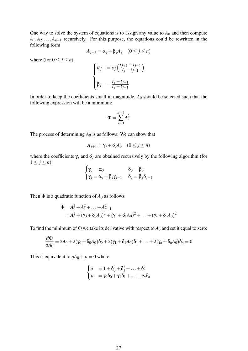
One way to solve the system of equations is to assign any value to A0 and then computeA1,A2, . . . ,An+1 recursively. For this purpose, the equations could be rewritten in thefollowing form

A j+1 = α j +β jA j (0≤ j ≤ n)

where (for 0≤ j ≤ n) α j = y j

(t j+1− t j−1t j− t j−1

)β j =

t j− t j+1t j− t j−1

In order to keep the coefficients small in magnitude, A0 should be selected such that thefollowing expression will be a minimum:

Φ =n+1

∑i=0

A2i

The process of determining A0 is as follows: We can show that

A j+1 = γ j +δ jA0 (0≤ j ≤ n)

where the coefficients γ j and δ j are obtained recursively by the following algorithm (for1≤ j ≤ n): {

γ0 = α0 δ0 = β0

γ j = α j +β jγ j−1 δ j = β jδ j−1

Then Φ is a quadratic function of A0 as follows:

Φ = A20 +A2

1 + . . .+A2n+1

= A20 +(γ0 +δ0A0)

2 +(γ1 +δ1A0)2 + . . .+(γn +δnA0)

2

To find the minimum of Φ we take its derivative with respect to A0 and set it equal to zero:

dΦ

dA0= 2A0 +2(γ0 +δ0A0)δ0 +2(γ1 +δ1A0)δ1 + . . .+2(γn +δnA0)δn = 0

This is equivalent to qA0 + p = 0 where{q = 1+δ2

0 +δ21 + . . .+δ2

n

p = γ0δ0 + γ1δ1 + . . .+ γnδn

27

Evaluation of the interpolating splineFinally, a set of results is quoted here in order to construct a procedure for evaluating S(x)once the coefficients Ai have been determined. The proof of these results is left as anexercise.

If the task is to evaluate the following second-degree spline

S(x) =∞

∑i=−∞

AiB2i−2(x)

at a given point x which lies in between the nodes t j−1 and t j, then we can calculate S(x)using the following equations

S(x) =1

t j− t j−1[d(x− t j−1)+ e(t j− x)]

where the functions d and e are given by

d =1

t j+1− t j−1[A j+1(x− t j−1)+A j(t j+1− x)]

ande =

1t j− t j−2

[A j(x− t j−2)+A j−1(t j− x)]

We are now ready to construct a program which calculates a quadratic spline interpolantfor a given set of data points.

28

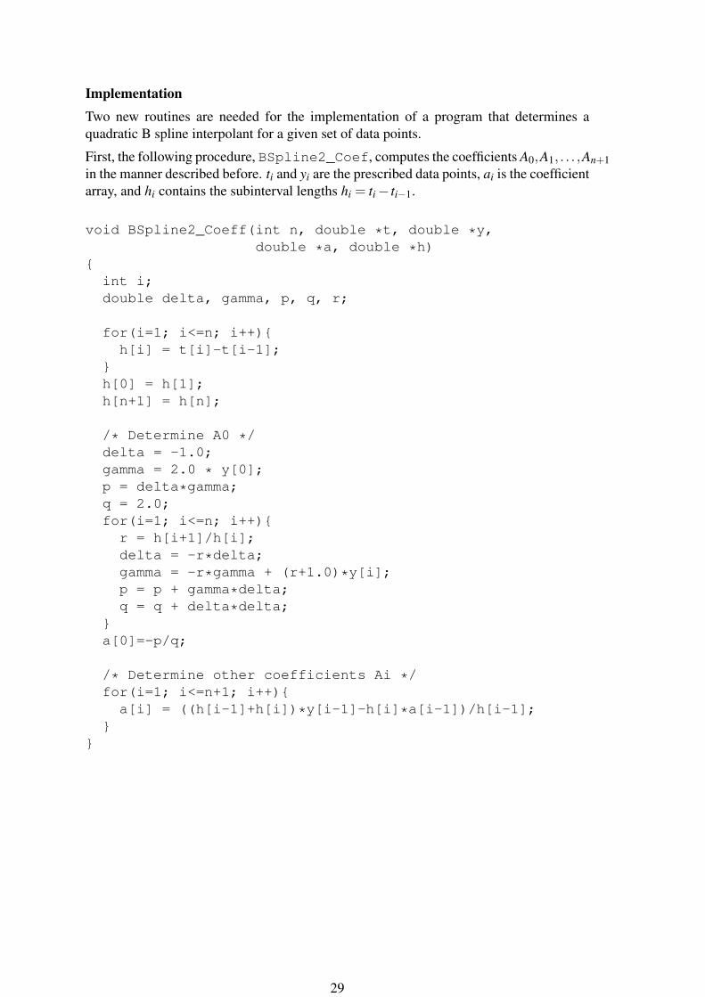
ImplementationTwo new routines are needed for the implementation of a program that determines aquadratic B spline interpolant for a given set of data points.

First, the following procedure, BSpline2_Coef, computes the coefficients A0,A1, . . . ,An+1in the manner described before. ti and yi are the prescribed data points, ai is the coefficientarray, and hi contains the subinterval lengths hi = ti− ti−1.

void BSpline2_Coeff(int n, double *t, double *y,double *a, double *h)

{int i;double delta, gamma, p, q, r;

for(i=1; i<=n; i++){h[i] = t[i]-t[i-1];

}h[0] = h[1];h[n+1] = h[n];

/* Determine A0 */delta = -1.0;gamma = 2.0 * y[0];p = delta*gamma;q = 2.0;for(i=1; i<=n; i++){

r = h[i+1]/h[i];delta = -r*delta;gamma = -r*gamma + (r+1.0)*y[i];p = p + gamma*delta;q = q + delta*delta;

}a[0]=-p/q;

/* Determine other coefficients Ai */for(i=1; i<=n+1; i++){

a[i] = ((h[i-1]+h[i])*y[i-1]-h[i]*a[i-1])/h[i-1];}

}

29

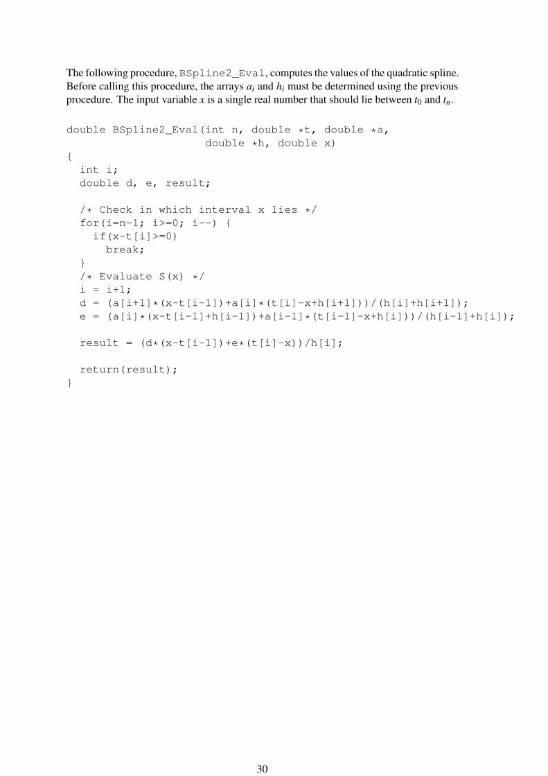
The following procedure, BSpline2_Eval, computes the values of the quadratic spline.Before calling this procedure, the arrays ai and hi must be determined using the previousprocedure. The input variable x is a single real number that should lie between t0 and tn.

double BSpline2_Eval(int n, double *t, double *a,double *h, double x)

{int i;double d, e, result;

/* Check in which interval x lies */for(i=n-1; i>=0; i--) {

if(x-t[i]>=0)break;

}/* Evaluate S(x) */i = i+1;d = (a[i+1]*(x-t[i-1])+a[i]*(t[i]-x+h[i+1]))/(h[i]+h[i+1]);e = (a[i]*(x-t[i-1]+h[i-1])+a[i-1]*(t[i-1]-x+h[i]))/(h[i-1]+h[i]);

result = (d*(x-t[i-1])+e*(t[i]-x))/h[i];

return(result);}

30

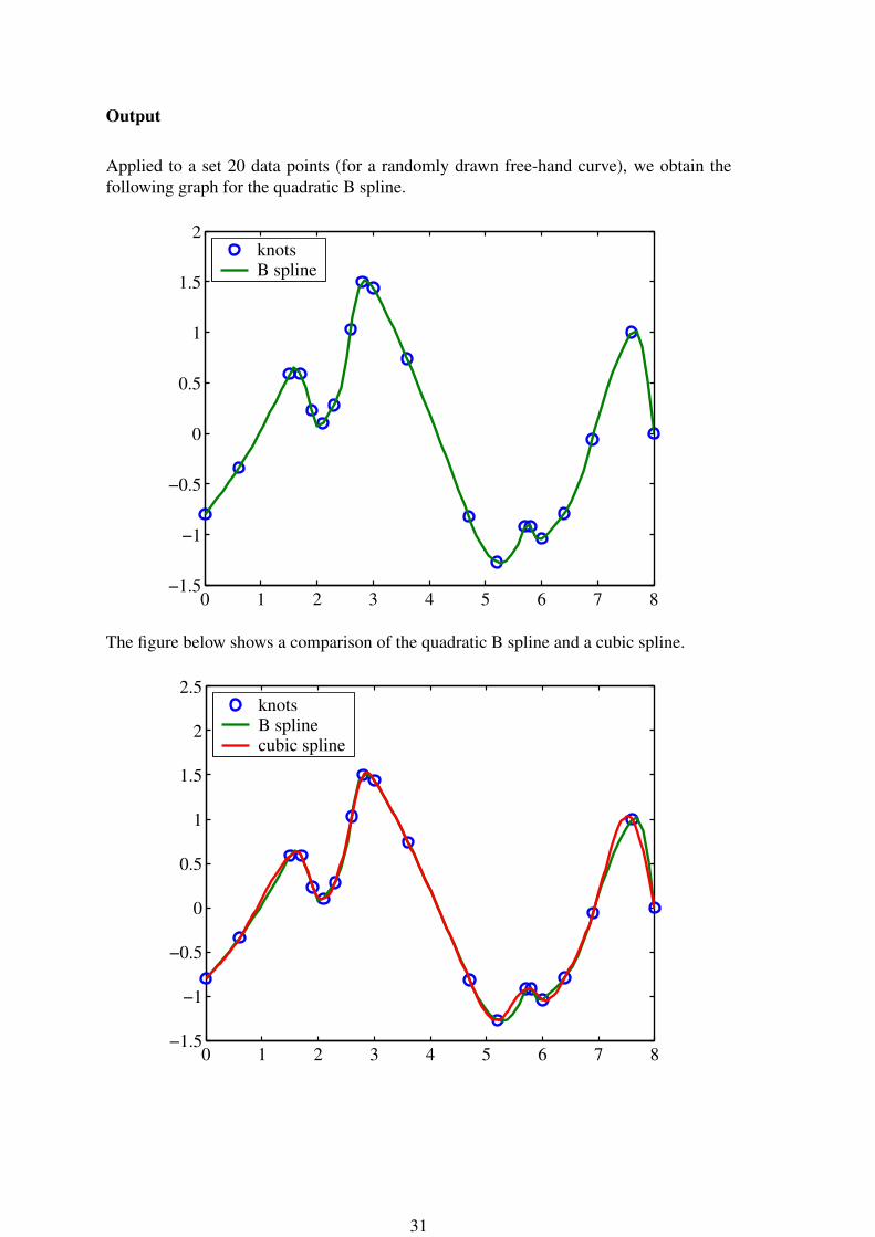
Output

Applied to a set 20 data points (for a randomly drawn free-hand curve), we obtain thefollowing graph for the quadratic B spline.

0 1 2 3 4 5 6 7 8−1.5

−1

−0.5

0

0.5

1

1.5

2knotsB spline

The figure below shows a comparison of the quadratic B spline and a cubic spline.

0 1 2 3 4 5 6 7 8−1.5

−1

−0.5

0

0.5

1

1.5

2

2.5knotsB splinecubic spline

31