Embed Size (px)
Citation preview

Lecture 4: Home Production and Labor Supply

Part 1:Labor Supply and Home Production
3
Simple Labor Supply Example: No Home Production
Look at static model:
1 1
( , )1 1
. .
. . .
:
:
C
N
C NU C N d
s t C wN
F O C
U C
U dN w
4
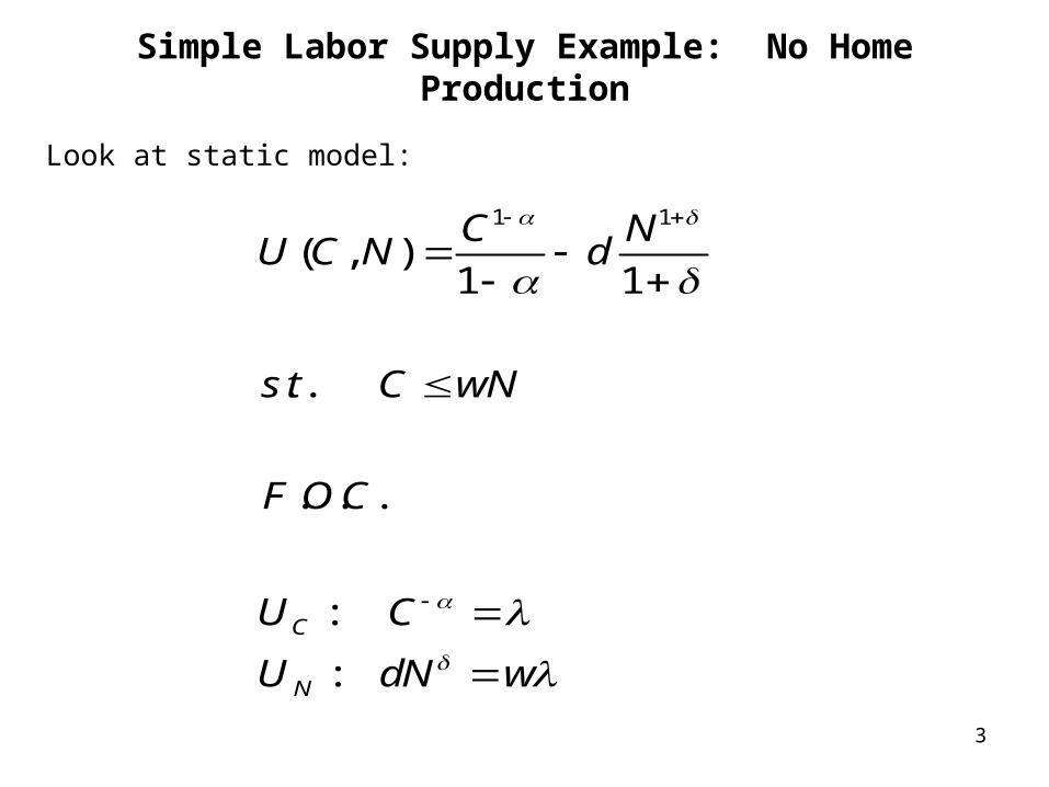
Simple Labor Supply Example: No Home Production
:
Take Logs:
1 1 1ln( ) ln( ) ln( ) ln( )
:
ln( ) ln( ) ln( )
NU dN w
N w d
Estimate
N A w
= labor supply elasticity with respect to wages (holding constant)
= labor supply elasticity with respect to marginal utility of wealth (holding w constant)
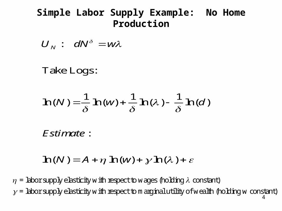
How Do Things Change With Home Production?
1 1
1/
1 1
1 1
( )( , )
1 1
. . X
( )
. . .
:
: ( )
: ( )
H X
C X
H H
N
C N HU C N d
s t wN
C H X
F O C
U C X
U C H d N H
U d N H w
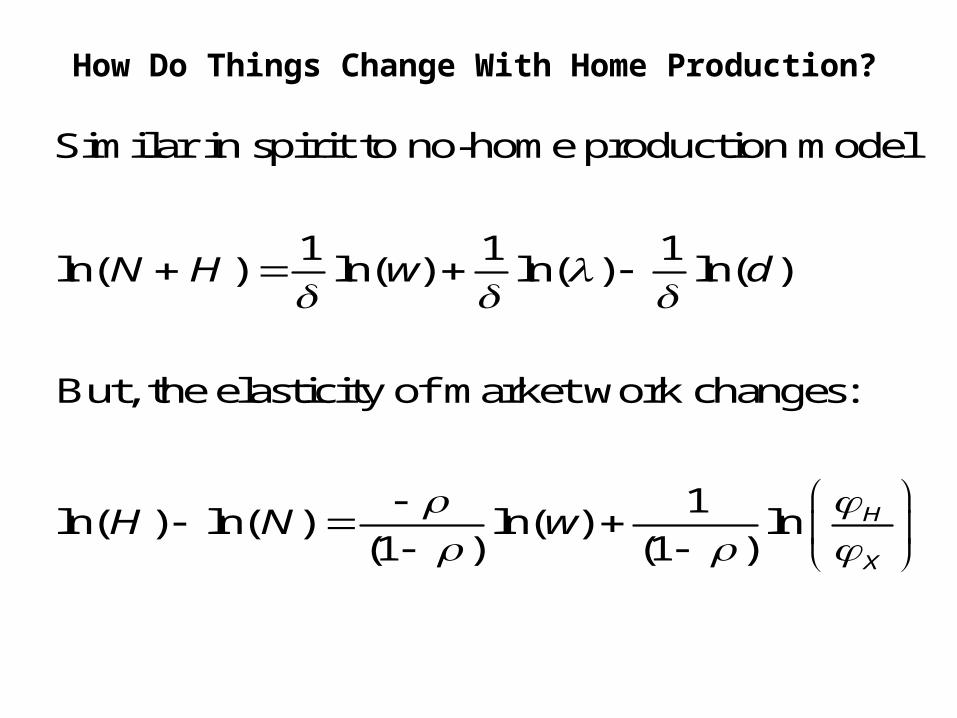
How Do Things Change With Home Production?
Similar in spirit to no-home production model
1 1 1ln( ) ln( ) ln( ) ln( )
But, the elasticity of market work changes:
1ln( ) ln( ) ln( ) ln
(1 ) (1 )H
X
N H w d
H N w
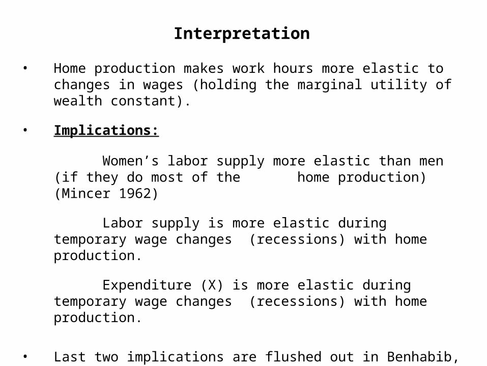
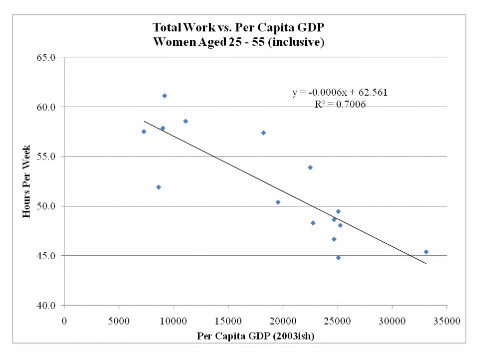
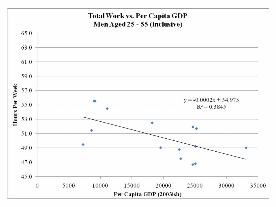
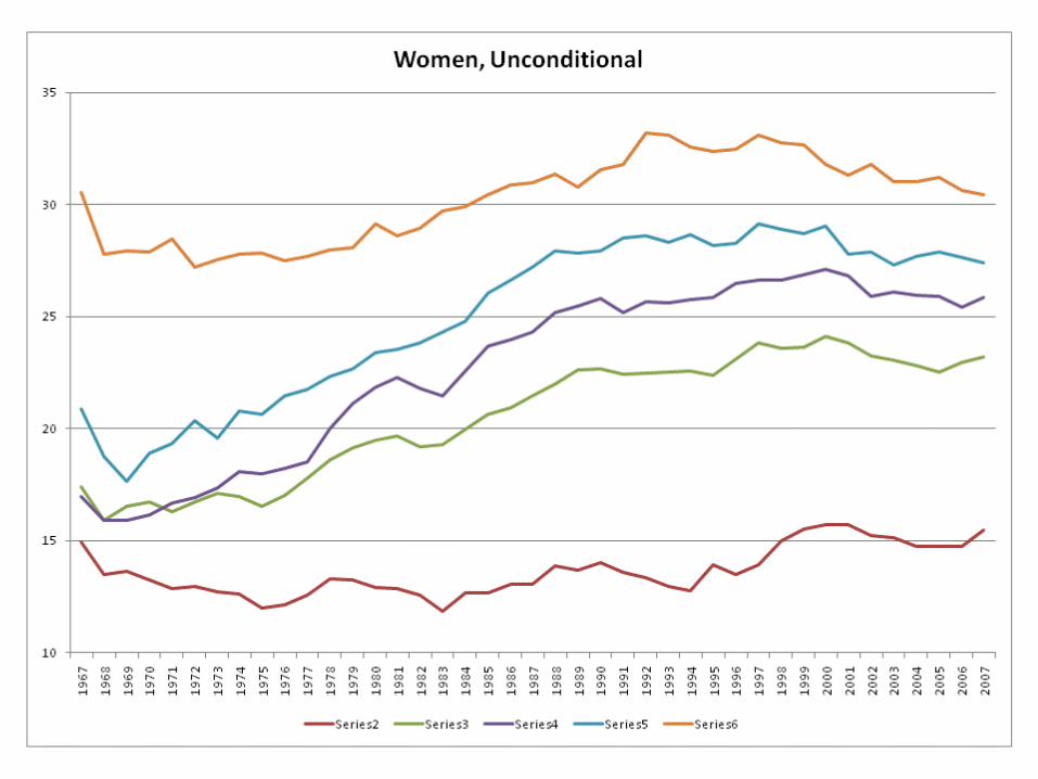
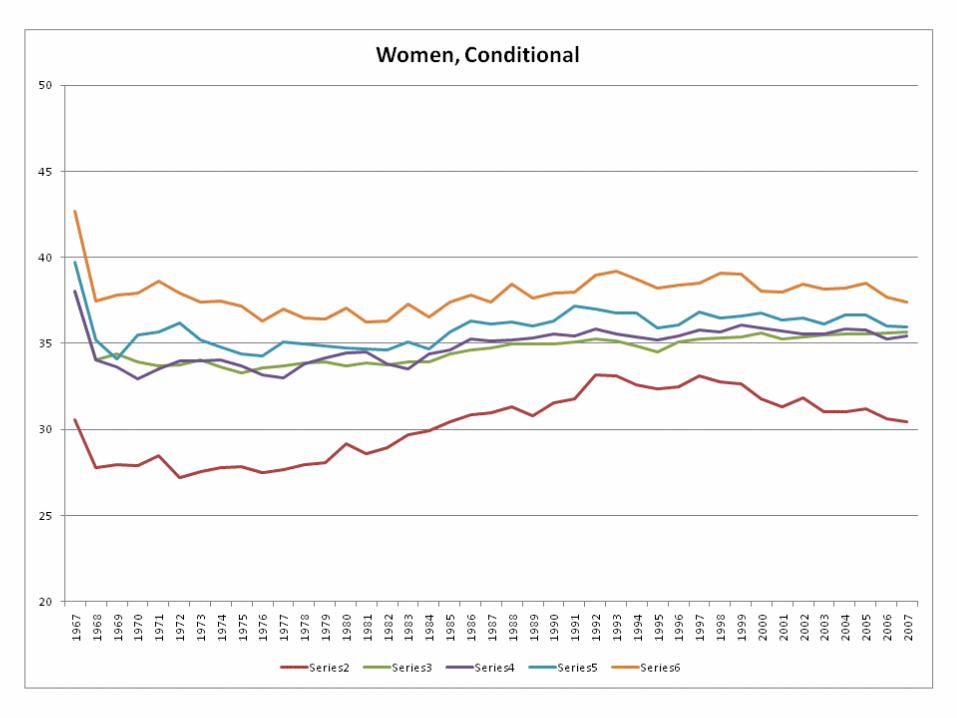
Interpretation
• Home production makes work hours more elastic to changes in wages (holding the marginal utility of wealth constant).
• Implications:
Women’s labor supply more elastic than men (if they do most of the home production) (Mincer 1962)
Labor supply is more elastic during temporary wage changes (recessions) with home production.
Expenditure (X) is more elastic during temporary wage changes (recessions) with home production.
• Last two implications are flushed out in Benhabib, Rogerson, and Wright’s “Home Work in Macroeconomics: Household Production and Aggregate Fluctuations” (JPE, 1991)
Part 2:Review of Trends in Leisure and Leisure
Inequality
Based on Aguiar and Hurst (2007, 2009)

Measures of Economic Inequality Have Increased Recently
• Wages (See Katz and Autor 1999)
• Consumption (Attanasio and Davis 1996 ; Attanasio et al. 2007)
• Consensus: “High Educated” standard of living has increased dramatically relative to “Low Educated”
standard of living since early 1980s
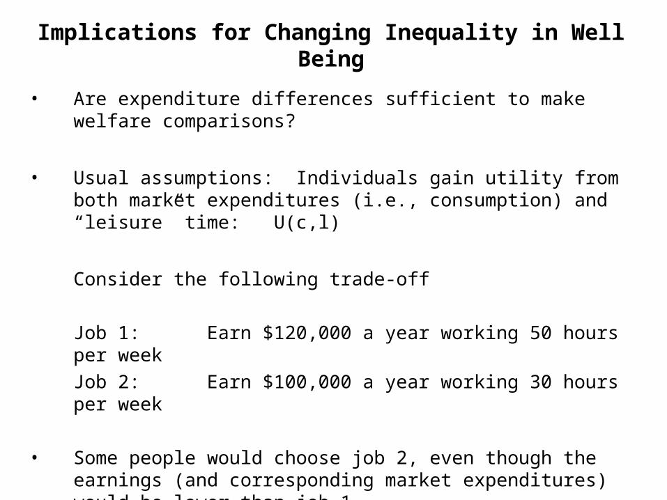
Implications for Changing Inequality in Well Being
• Are expenditure differences sufficient to make welfare comparisons?
• Usual assumptions: Individuals gain utility from both market expenditures (i.e., consumption) and “leisure” time: U(c,l)
Consider the following trade-off
Job 1: Earn $120,000 a year working 50 hours per week
Job 2: Earn $100,000 a year working 30 hours per week
• Some people would choose job 2, even though the earnings (and corresponding market expenditures) would be lower than job 1.
• People “value” time.

What We Do in this Paper
• Explore the changing nature of the allocation of time over the last 40 years.
– Focus on the aggregate trends.
– Examine the changing nature of “leisure inequality”.
• Ask a related question: Can changing educational differences in employment status explain changing leisure inequality?
• Why is that interesting? In terms of welfare implications, it is important to know whether low education individuals are taking more leisure because they are unable to find employment at their reservation wage. (Individuals will be off their labor supply curve).

Key Finding
• Leisure inequality has increased dramatically since 1985
– Relative to high educated men, low educated men have gained an additional 7 hours per week of leisure!
• At most, only 40% of the increase in leisure inequality can be explained by the potential of involuntary unemployment (including disability) of low educated men.
– This is an upper bound.
Some low educated men are out of the labor force by choice.
Some high educated men are involuntarily unemployed.
• Take Away: Need to think about how to measure changing relative well being between high and low educated men since 1985.
13
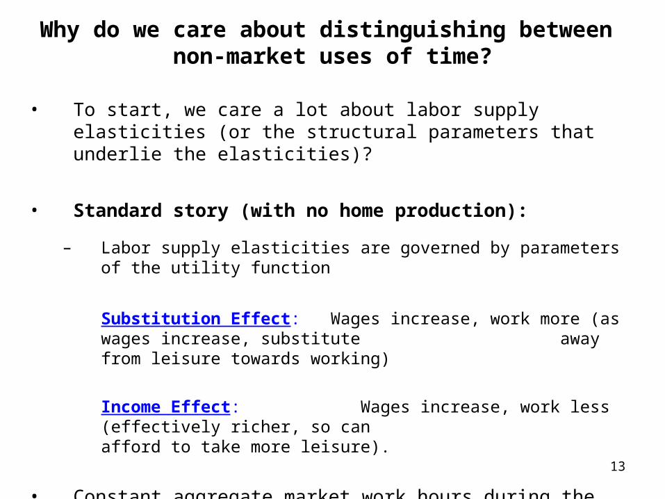
Why do we care about distinguishing between non-market uses of time?
• To start, we care a lot about labor supply elasticities (or the structural parameters that underlie the elasticities)?
• Standard story (with no home production):
– Labor supply elasticities are governed by parameters of the utility function
Substitution Effect: Wages increase, work more (as wages increase, substitute away from leisure towards working)
Income Effect: Wages increase, work less (effectively richer, so can afford to take more leisure).
• Constant aggregate market work hours during the last forty years as wages have increased has been interpreted as income and substitution effects (determined by these preference parameters) canceling.
14
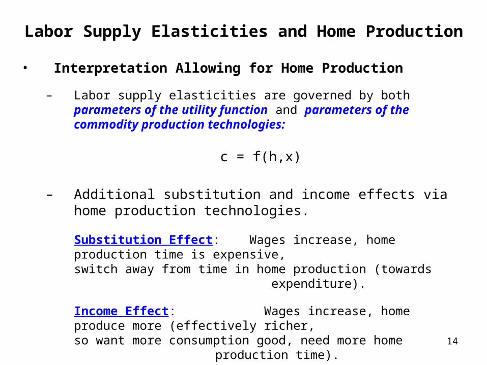
Labor Supply Elasticities and Home Production
• Interpretation Allowing for Home Production
– Labor supply elasticities are governed by both parameters of the utility function and parameters of the commodity production technologies:
c = f(h,x)
– Additional substitution and income effects via home production technologies.
Substitution Effect: Wages increase, home production time is expensive, switch away from time in home production
(towards expenditure).
Income Effect: Wages increase, home produce more (effectively richer, so want more consumption good, need more
home production time).
– Note, by definition, Leisure goods have little (if any) substitution effects
15
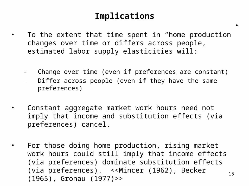
Implications
• To the extent that time spent in “home production” changes over time or differs across people, estimated labor supply elasticities will:
– Change over time (even if preferences are constant)
– Differ across people (even if they have the same preferences)
• Constant aggregate market work hours need not imply that income and substitution effects (via preferences) cancel.
• For those doing home production, rising market work hours could still imply that income effects (via preferences) dominate substitution effects (via preferences). <<Mincer (1962), Becker (1965), Gronau (1977)>>
• Can learn about preferences, the home production technologies and the leisure technologies by jointly examining the behavior of home production, leisure, and market work.
16
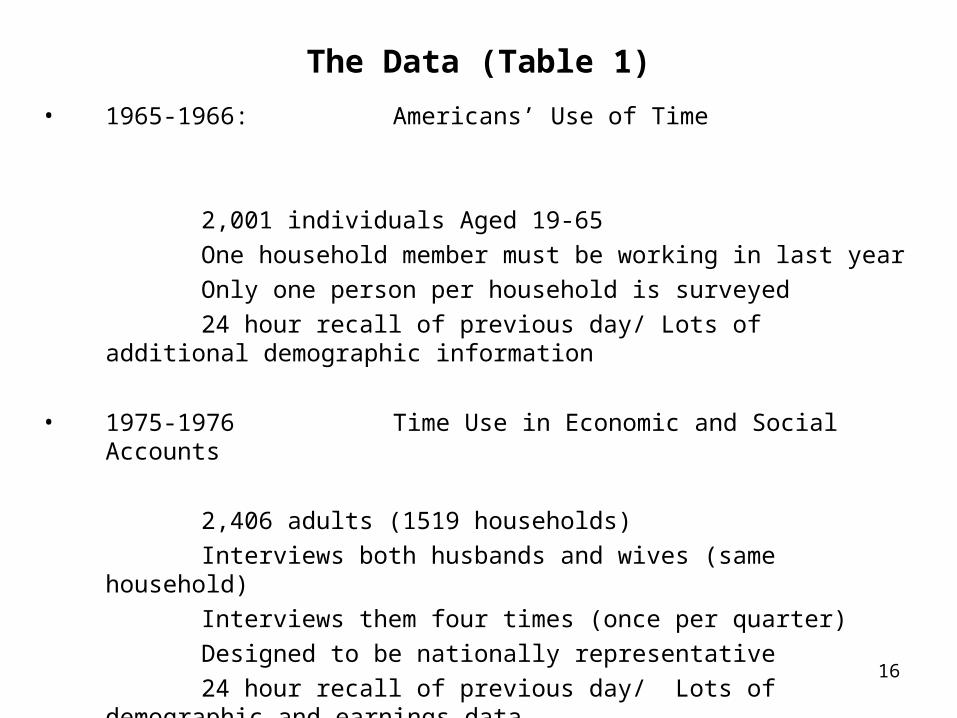
The Data (Table 1)
• 1965-1966: Americans’ Use of Time
2,001 individuals Aged 19-65
One household member must be working in last year
Only one person per household is surveyed
24 hour recall of previous day/ Lots of additional demographic information
• 1975-1976 Time Use in Economic and Social Accounts
2,406 adults (1519 households)
Interviews both husbands and wives (same household)
Interviews them four times (once per quarter)
Designed to be nationally representative
24 hour recall of previous day/ Lots of demographic and earnings data
Note: We only use first interview (fall 1975)
17
The Data (Table 1)
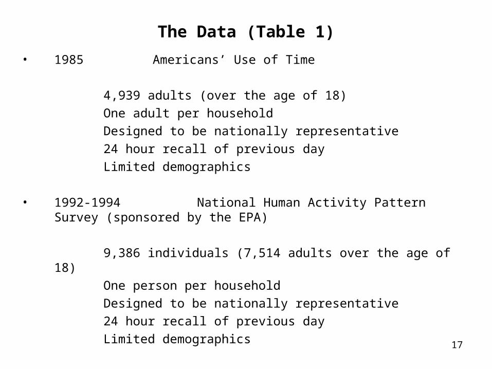
• 1985 Americans’ Use of Time
4,939 adults (over the age of 18)
One adult per household
Designed to be nationally representative
24 hour recall of previous day
Limited demographics
• 1992-1994 National Human Activity Pattern Survey (sponsored by the EPA)
9,386 individuals (7,514 adults over the age of 18)
One person per household
Designed to be nationally representative
24 hour recall of previous day
Limited demographics
18
The Data (Table 1)
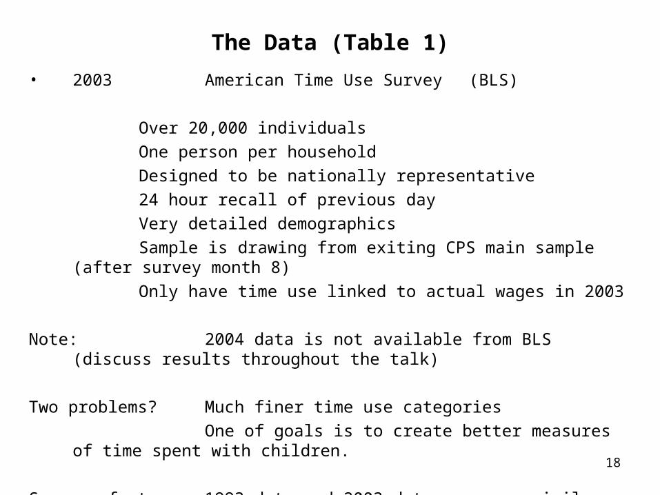
• 2003 American Time Use Survey (BLS)
Over 20,000 individuals
One person per household
Designed to be nationally representative
24 hour recall of previous day
Very detailed demographics
Sample is drawing from exiting CPS main sample (after survey month 8)
Only have time use linked to actual wages in 2003
Note: 2004 data is not available from BLS (discuss results throughout the talk)
Two problems? Much finer time use categories
One of goals is to create better measures of time spent with children.
Some comfort: 1993 data and 2003 data are very similar along many dimensions
19
Some Existing Work on Time Use
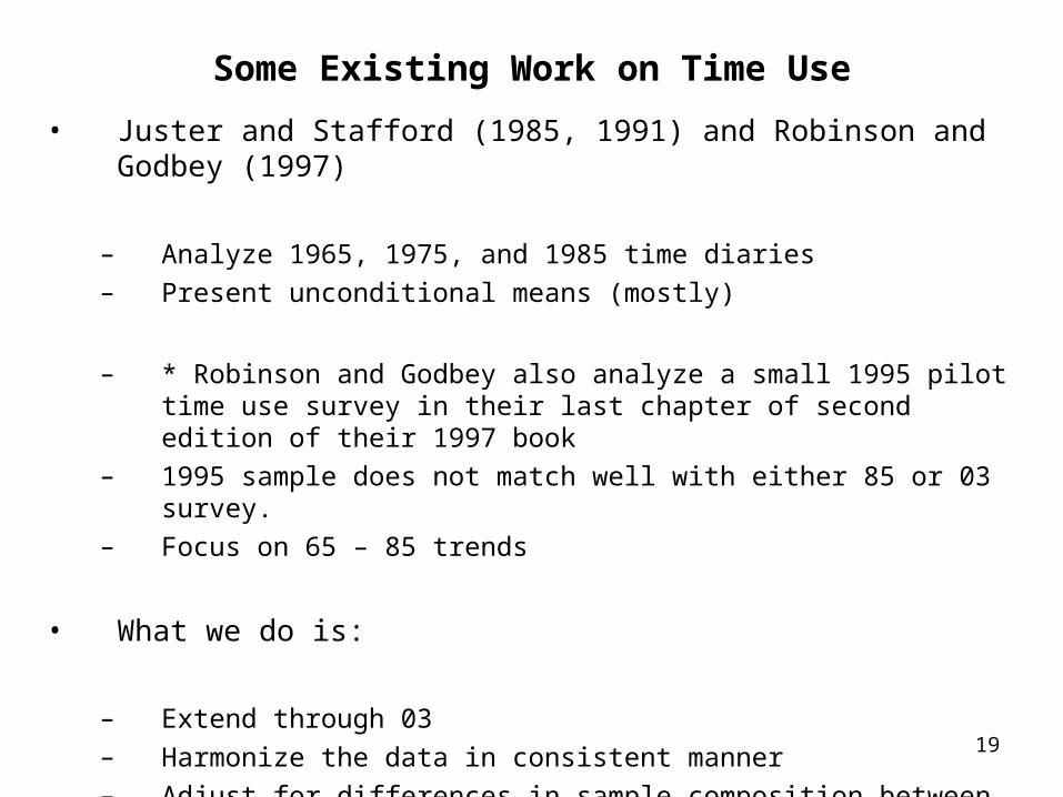
• Juster and Stafford (1985, 1991) and Robinson and Godbey (1997)
– Analyze 1965, 1975, and 1985 time diaries
– Present unconditional means (mostly)
– * Robinson and Godbey also analyze a small 1995 pilot time use survey in their last chapter of second edition of their 1997 book
– 1995 sample does not match well with either 85 or 03 survey.
– Focus on 65 – 85 trends
• What we do is:
– Extend through 03
– Harmonize the data in consistent manner
– Adjust for differences in sample composition between surveys
– Also show conditional means.
20
Creating consistent measures of Time Use
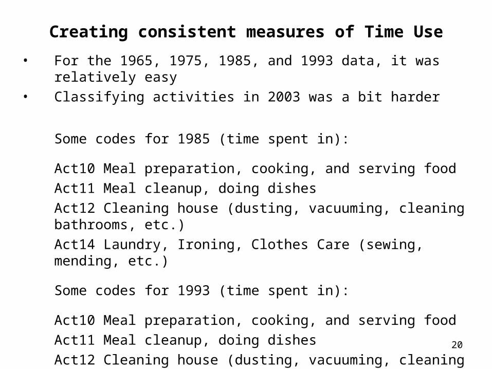
• For the 1965, 1975, 1985, and 1993 data, it was relatively easy
• Classifying activities in 2003 was a bit harder
Some codes for 1985 (time spent in):
Act10 Meal preparation, cooking, and serving food
Act11 Meal cleanup, doing dishes
Act12 Cleaning house (dusting, vacuuming, cleaning bathrooms, etc.)
Act14 Laundry, Ironing, Clothes Care (sewing, mending, etc.)
Some codes for 1993 (time spent in):
Act10 Meal preparation, cooking, and serving food
Act11 Meal cleanup, doing dishes
Act12 Cleaning house (dusting, vacuuming, cleaning bathrooms, etc.)
Act14 Laundry, Ironing, Clothes Care (sewing, mending, etc.)
21
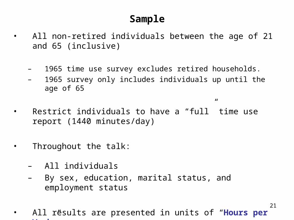
Sample
• All non-retired individuals between the age of 21 and 65 (inclusive)
– 1965 time use survey excludes retired households.
– 1965 survey only includes individuals up until the age of 65
• Restrict individuals to have a “full” time use report (1440 minutes/day)
• Throughout the talk:
– All individuals
– By sex, education, marital status, and employment status
• All results are presented in units of “Hours per Week”
22
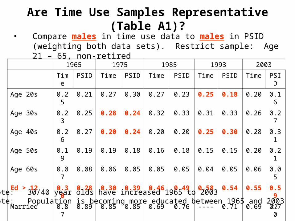
Are Time Use Samples Representative (Table A1)?• Compare males in time use data to males in PSID (weighting both data
sets). Restrict sample: Age 21 – 65, non-retired
1965 1975 1985 1993 2003
Time PSID Time PSID Time PSID Time PSID Time PSID
Age 20s 0.25 0.21 0.27 0.30 0.27 0.23 0.25 0.18 0.20 0.16
Age 30s 0.23 0.25 0.28 0.24 0.32 0.33 0.31 0.33 0.26 0.27
Age 40s 0.26 0.27 0.20 0.24 0.20 0.20 0.25 0.30 0.28 0.31
Age 50s 0.19 0.19 0.19 0.18 0.16 0.18 0.15 0.15 0.20 0.21
Age 60s 0.07 0.08 0.06 0.05 0.05 0.05 0.04 0.05 0.06 0.05
Ed > 12 0.30 0.28 0.30 0.39 0.46 0.49 0.58 0.54 0.55 0.59
Married 0.87 0.89 0.85 0.85 0.69 0.76 ---- 0.71 0.69 0.70
Have Kid 0.65 0.65 0.55 0.60 0.42 0.51 0.32 0.46 0.42 0.45
# of Kids
Employed
1.57
0.97
1.66
0.96
1.24
0.93
1.30
0.93
0.76
0.88
0.96
0.90
----
0.89
0.89
0.91
0.80
0.88
0.86
0.91
• Note: 30/40 year olds have increased 1965 to 2003• Note: Population is becoming more educated between 1965 and 2003
23
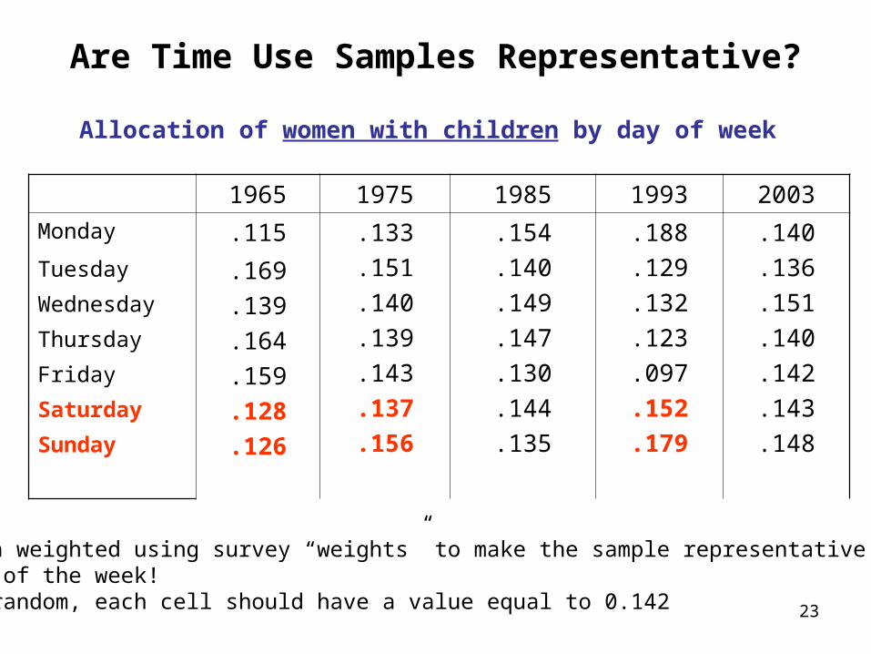
Are Time Use Samples Representative?
1965 1975 1985 1993 2003
Monday .115 .133
.151
.140
.139
.143
.137
.156
.154
.140
.149
.147
.130
.144
.135
.188
.129
.132
.123
.097
.152
.179
.140
.136
.151
.140
.142
.143
.148
Tuesday .169
.139
.164
.159
.128
.126
Wednesday
Thursday
Friday
Saturday
Sunday
• Data weighted using survey “weights” to make the sample representative by day of the week!
• If random, each cell should have a value equal to 0.142
Allocation of women with children by day of week
24
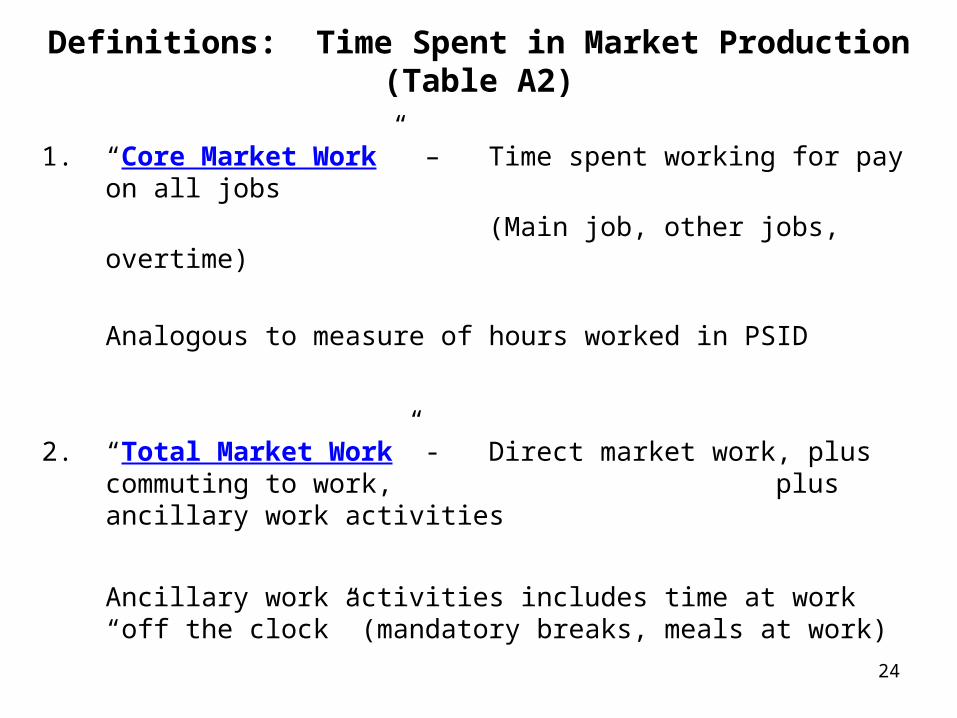
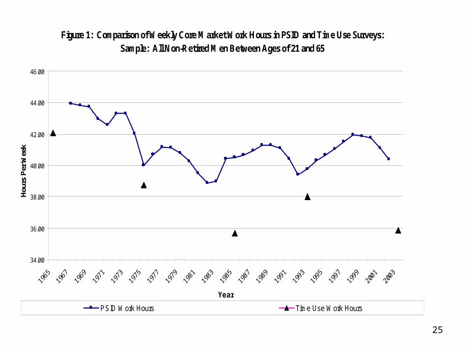
Definitions: Time Spent in Market Production (Table A2)
1. “Core Market Work” – Time spent working for pay on all jobs
(Main job, other jobs, overtime)
Analogous to measure of hours worked in PSID
2. “Total Market Work” - Direct market work, plus commuting to work, plus ancillary work activities
Ancillary work activities includes time at work “off the clock” (mandatory breaks, meals at work)
25
Figure 1: Comparison of Weekly Core Market Work Hours in PSID and Time Use Surveys: Sample: All Non-Retired Men Between Ages of 21 and 65
34.00
36.00
38.00
40.00
42.00
44.00
46.00
Year
Hou
rs P
er W
eek
PSID Work Hours Time Use Work Hours
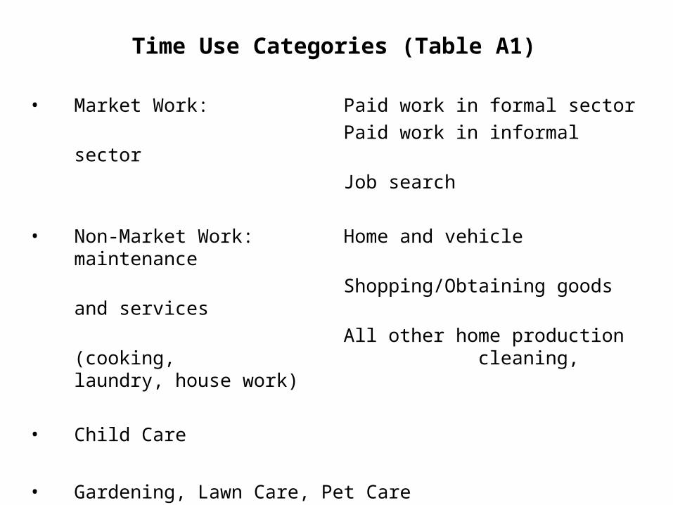
Time Use Categories (Table A1)
• Market Work: Paid work in formal sector
Paid work in informal sector
Job search
• Non-Market Work: Home and vehicle maintenance
Shopping/Obtaining goods and services
All other home production (cooking, cleaning, laundry, house work)
• Child Care
• Gardening, Lawn Care, Pet Care
Note: All associated travel time is embedded in the time use category
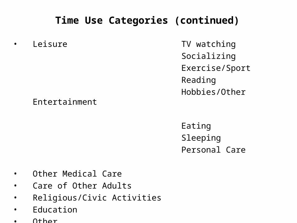
Time Use Categories (continued)
• Leisure TV watching
Socializing
Exercise/Sport
Reading
Hobbies/Other Entertainment
Eating
Sleeping
Personal Care
• Other Medical Care
• Care of Other Adults
• Religious/Civic Activities
• Education
• Other
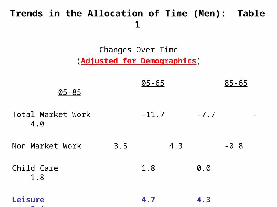
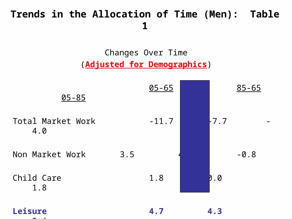
Trends in the Allocation of Time (Men): Table 1
Changes Over Time
(Adjusted for Demographics)
05-65 85-65 05-85
Total Market Work -11.7 -7.7 -4.0
Non Market Work 3.5 4.3 -0.8
Child Care 1.8 0.0 1.8
Leisure 4.7 4.3 0.4
Trends in the Allocation of Time (Men): Table 1
Changes Over Time
(Adjusted for Demographics)
05-65 85-65 05-85
Total Market Work -11.7 -7.7 -4.0
Non Market Work 3.5 4.3 -0.8
Child Care 1.8 0.0 1.8
Leisure 4.7 4.3 0.4
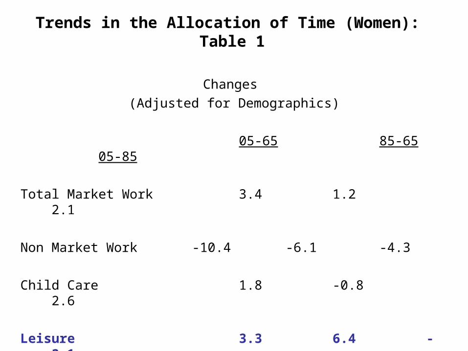
Trends in the Allocation of Time (Women): Table 1
Changes
(Adjusted for Demographics)
05-65 85-65 05-85
Total Market Work 3.4 1.2 2.1
Non Market Work -10.4 -6.1 -4.3
Child Care 1.8 -0.8 2.6
Leisure 3.3 6.4 -3.1
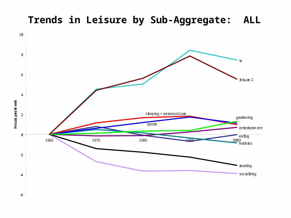
Trends in Leisure by Sub-Aggregate: ALL
tv
socializing
entertainment
hobbies
reading
eating
sleeping + personal care
sports
gardening
leisure 2
-6
-4
-2
0
2
4
6
8
10
1965 1975 1985 1993 2003
Ho
urs
per
Wee
k
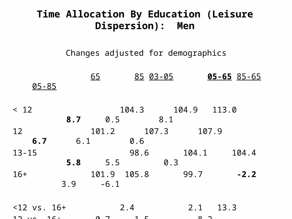
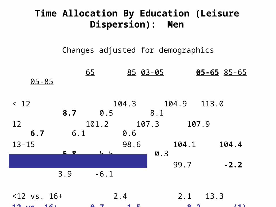
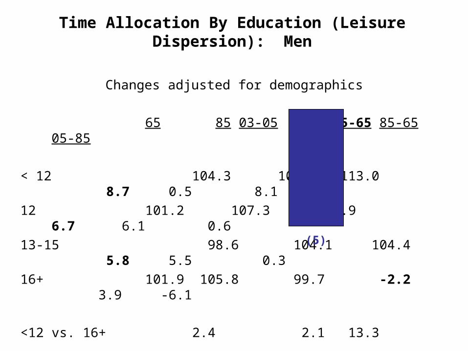
Time Allocation By Education (Leisure Dispersion): Men
Changes adjusted for demographics
65 85 03-05 05-65 85-65 05-85
< 12 104.3 104.9 113.0 8.7 0.5 8.1
12 101.2 107.3 107.9 6.7 6.1 0.6
13-15 98.6 104.1 104.4 5.8 5.5 0.3
16+ 101.9 105.8 99.7 -2.2 3.9 -6.1
<12 vs. 16+ 2.4 2.1 13.3
12 vs. 16+ -0.7 1.5 8.2
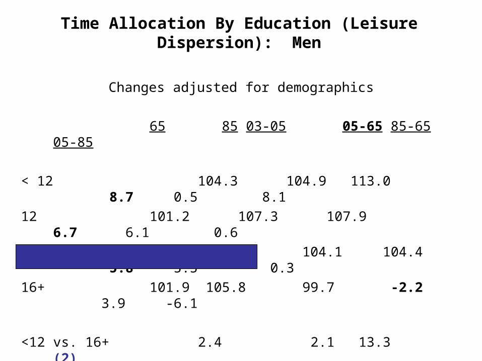
Time Allocation By Education (Leisure Dispersion): Men
Changes adjusted for demographics
65 85 03-05 05-65 85-65 05-85
< 12 104.3 104.9 113.0 8.7 0.5 8.1
12 101.2 107.3 107.9 6.7 6.1 0.6
13-15 98.6 104.1 104.4 5.8 5.5 0.3
16+ 101.9 105.8 99.7 -2.2 3.9 -6.1
<12 vs. 16+ 2.4 2.1 13.3
12 vs. 16+ -0.7 1.5 8.2 (1)
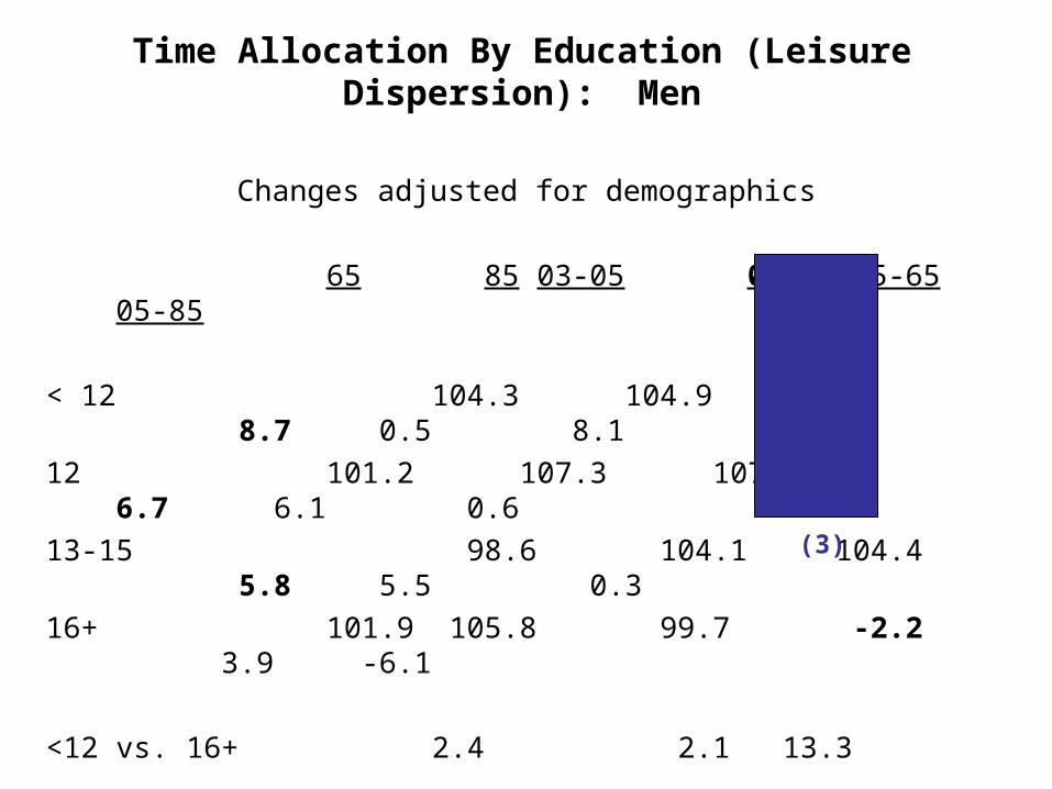
Time Allocation By Education (Leisure Dispersion): Men
Changes adjusted for demographics
65 85 03-05 05-65 85-65 05-85
< 12 104.3 104.9 113.0 8.7 0.5 8.1
12 101.2 107.3 107.9 6.7 6.1 0.6
13-15 98.6 104.1 104.4 5.8 5.5 0.3
16+ 101.9 105.8 99.7 -2.2 3.9 -6.1
<12 vs. 16+ 2.4 2.1 13.3 (2)
12 vs. 16+ -0.7 1.5 8.2
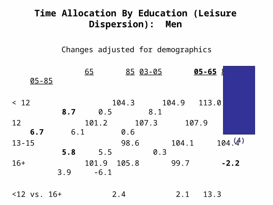
Time Allocation By Education (Leisure Dispersion): Men
Changes adjusted for demographics
65 85 03-05 05-65 85-65 05-85
< 12 104.3 104.9 113.0 8.7 0.5 8.1
12 101.2 107.3 107.9 6.7 6.1 0.6
13-15 98.6 104.1 104.4 5.8 5.5 0.3
16+ 101.9 105.8 99.7 -2.2 3.9 -6.1
<12 vs. 16+ 2.4 2.1 13.3
12 vs. 16+ -0.7 1.5 8.2
(3)
Time Allocation By Education (Leisure Dispersion): Men
Changes adjusted for demographics
65 85 03-05 05-65 85-65 05-85
< 12 104.3 104.9 113.0 8.7 0.5 8.1
12 101.2 107.3 107.9 6.7 6.1 0.6
13-15 98.6 104.1 104.4 5.8 5.5 0.3
16+ 101.9 105.8 99.7 -2.2 3.9 -6.1
<12 vs. 16+ 2.4 2.1 13.3
12 vs. 16+ -0.7 1.5 8.2
(4)
Time Allocation By Education (Leisure Dispersion): Men
Changes adjusted for demographics
65 85 03-05 05-65 85-65 05-85
< 12 104.3 104.9 113.0 8.7 0.5 8.1
12 101.2 107.3 107.9 6.7 6.1 0.6
13-15 98.6 104.1 104.4 5.8 5.5 0.3
16+ 101.9 105.8 99.7 -2.2 3.9 -6.1
<12 vs. 16+ 2.4 2.1 13.3
12 vs. 16+ -0.7 1.5 8.2
(5)

Time Allocation By Education (Leisure Dispersion): Men
Changes adjusted for demographics
65 85 03-05 05-65 85-65 05-85
< 12 104.3 104.9 113.0 8.7 0.5 8.1
12 101.2 107.3 107.9 6.7 6.1 0.6
13-15 98.6 104.1 104.4 5.8 5.5 0.3
16+ 101.9 105.8 99.7 -2.2 3.9 -6.1
<12 vs. 16+ 2.4 2.1 13.3
12 vs. 16+ -0.7 1.5 8.2
Question: Is the dispersion driven by the changing pool of individuals within each educational category?
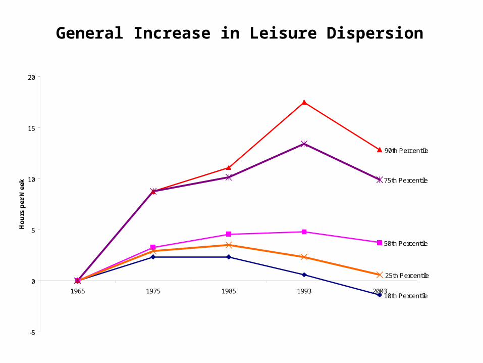
General Increase in Leisure Dispersion
10th Percentile
50th Percentile
90th Percentile
25th Percentile
75th Percentile
-5
0
5
10
15
20
1965 1975 1985 1993 2003
Ho
urs
per
Wee
k
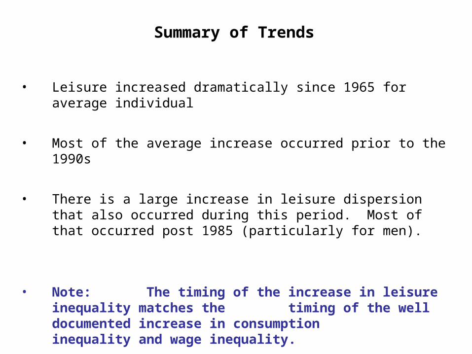
Summary of Trends
• Leisure increased dramatically since 1965 for average individual
• Most of the average increase occurred prior to the 1990s
• There is a large increase in leisure dispersion that also occurred during this period. Most of that occurred post 1985 (particularly for men).
• Note: The timing of the increase in leisure inequality matches the timing of the well documented increase in
consumption inequality and wage inequality.
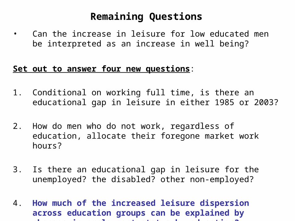
Remaining Questions
• Can the increase in leisure for low educated men be interpreted as an increase in well being?
Set out to answer four new questions:
1. Conditional on working full time, is there an educational gap in leisure in either 1985 or 2003?
2. How do men who do not work, regardless of education, allocate their foregone market work hours?
3. Is there an educational gap in leisure for the unemployed? the disabled? other non-employed?
4. How much of the increased leisure dispersion across education groups can be explained by changes in employment status by education?

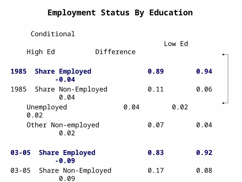
Employment Status By Education
Conditional
Low Ed High Ed Difference
1985 Share Employed 0.89 0.94 -0.04
1985 Share Non-Employed 0.11 0.06 0.04
Unemployed 0.04 0.02 0.02
Other Non-employed 0.07 0.04 0.02
03-05 Share Employed 0.83 0.92 -0.09
03-05 Share Non-Employed 0.17 0.08 0.09
Unemployed 0.05 0.04 0.02
Disabled 0.08 0.02 0.05
Other Non-employed 0.04 0.03 0.02
Note: From now on, we only focus on two education groups (because of small sample sizes in some cells).
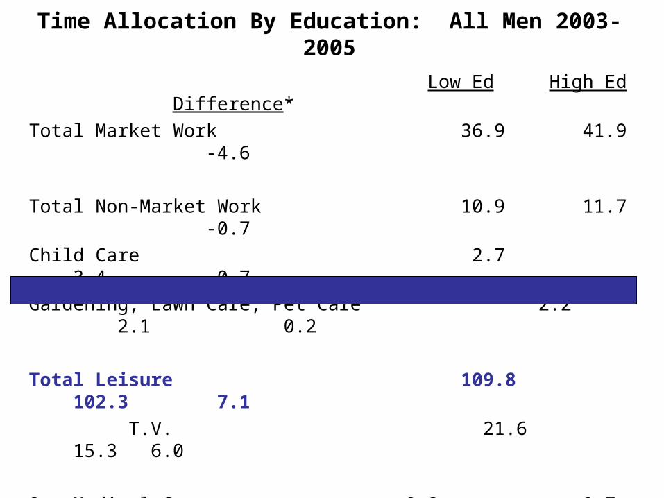
Time Allocation By Education: All Men 2003-2005
Low Ed High Ed Difference*
Total Market Work 36.9 41.9 -4.6
Total Non-Market Work 10.9 11.7 -0.7
Child Care 2.7 3.4 -0.7
Gardening, Lawn Care, Pet Care 2.2 2.1 0.2
Total Leisure 109.8 102.3 7.1
T.V. 21.6 15.3 6.0
Own Medical Care 0.8 0.7 0.1
Care of Other Adults 1.7 1.4 0.2
Religious/Civic Activities 1.5 1.9 -0.4
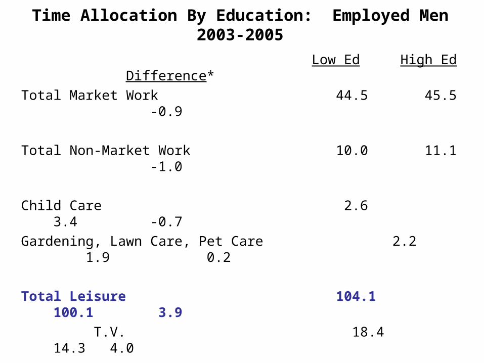
Time Allocation By Education: Employed Men 2003-2005
Low Ed High Ed Difference*
Total Market Work 44.5 45.5 -0.9
Total Non-Market Work 10.0 11.1 -1.0
Child Care 2.6 3.4 -0.7
Gardening, Lawn Care, Pet Care 2.2 1.9 0.2
Total Leisure 104.1 100.1 3.9
T.V. 18.4 14.3 4.0
Own Medical Care 0.5 0.6 -0.1
Care of Other Adults 1.6 1.3 0.3
Religious/Civic Activities 1.3 1.8 -0.5
* Conditional on Demographics
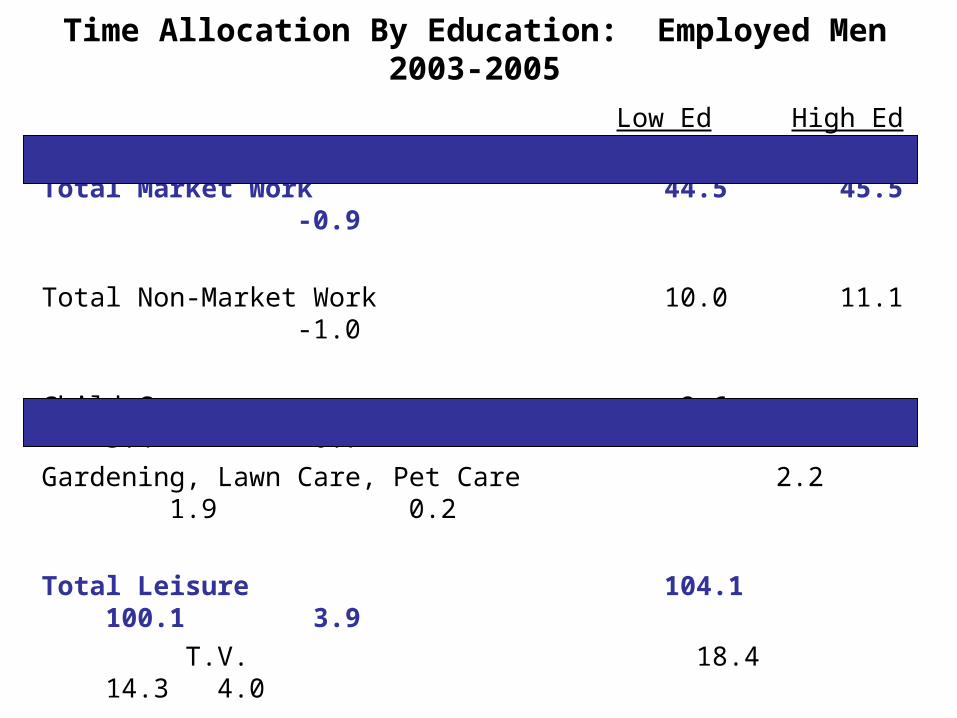
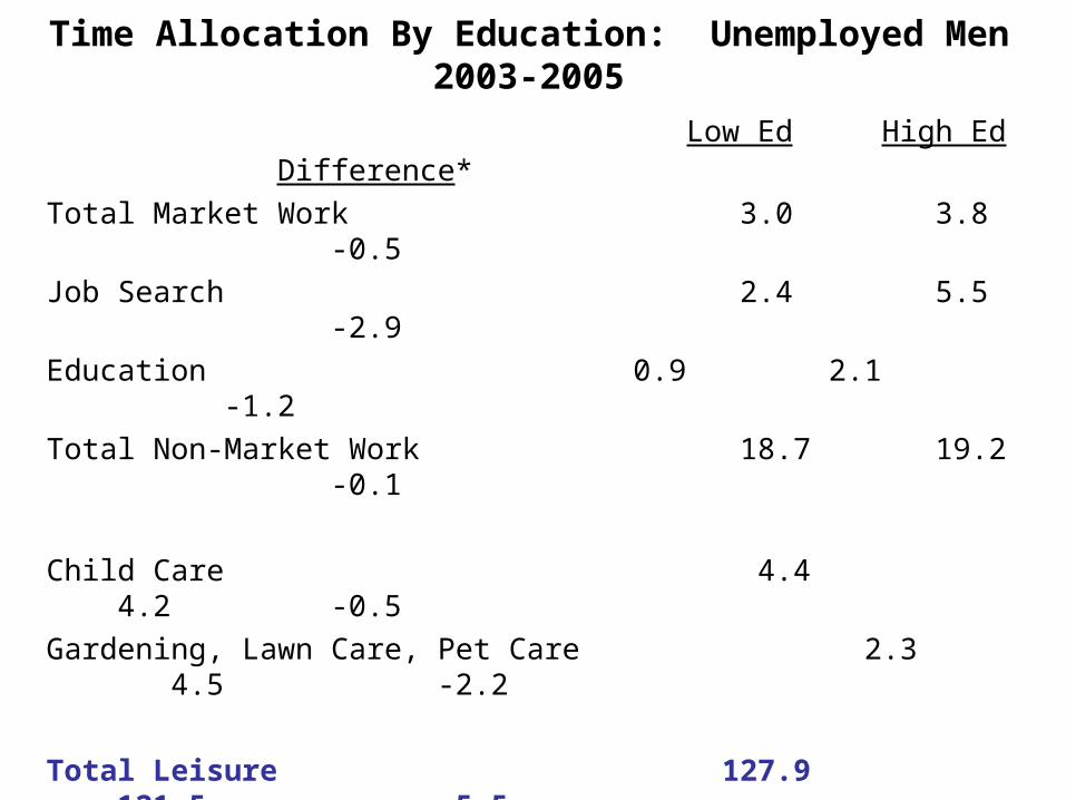
Time Allocation By Education: Unemployed Men 2003-2005
Low Ed High Ed Difference*
Total Market Work 3.0 3.8 -0.5
Job Search 2.4 5.5 -2.9
Education 0.9 2.1 -1.2
Total Non-Market Work 18.7 19.2 -0.1
Child Care 4.4 4.2 -0.5
Gardening, Lawn Care, Pet Care 2.3 4.5 -2.2
Total Leisure 127.9 121.5 5.5
T.V. 29.7 22.2 7.5
Own Medical Care 0.6 0.5 0.2
Care of Other Adults 3.0 2.4 0.8
Religious/Civic Activities 2.4 2.6 0.1
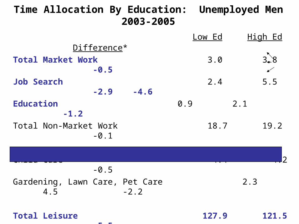
Time Allocation By Education: Unemployed Men 2003-2005
Low Ed High Ed Difference*
Total Market Work 3.0 3.8 -0.5
Job Search 2.4 5.5 -2.9 -4.6
Education 0.9 2.1 -1.2
Total Non-Market Work 18.7 19.2 -0.1
Child Care 4.4 4.2 -0.5
Gardening, Lawn Care, Pet Care 2.3 4.5 -2.2
Total Leisure 127.9 121.5 5.5
T.V. 29.7 22.2 7.5
Own Medical Care 0.6 0.5 0.2
Care of Other Adults 3.0 2.4 0.8
Religious/Civic Activities 2.4 2.6 0.1

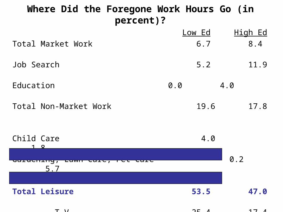
Where Did the Foregone Work Hours Go (in percent)?
Low Ed High Ed
Total Market Work 6.7 8.4
Job Search 5.2 11.9
Education 0.0 4.0
Total Non-Market Work 19.6 17.8
Child Care 4.0 1.8
Gardening, Lawn Care, Pet Care 0.2 5.7
Total Leisure 53.5 47.0
T.V. 25.4 17.4
Socialization 12.6 8.4
Sleeping 12.6 10.1
Other Entertainment/Hobbies -0.7 8.6
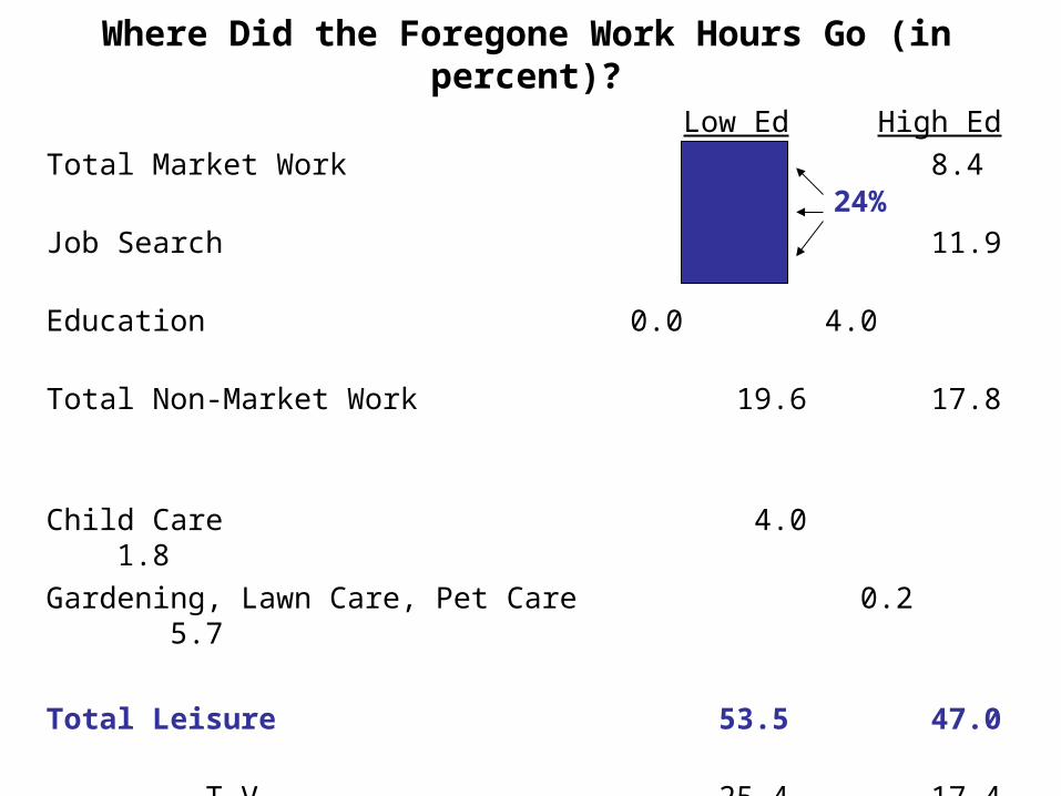
24%

Time Allocation By Education: Disabled Men 2003-2005
Low Ed High Ed Difference*
Total Market Work 0.0 0.7 -0.7
Job Search 0.0 0.2 -0.2
Education 0.2 1.6 -1.7
Total Non-Market Work 10.6 12.8 -1.8
Child Care 2.5 2.0 0.2
Gardening, Lawn Care, Pet Care 2.2 1.3 1.0
Total Leisure 144.1 138.7 5.7
T.V. 43.2 36.0 7.5
Own Medical Care 4.3 4.6 -0.5
Care of Other Adults 1.5 2.5 -1.4
Religious/Civic Activities 2.2 2.1 0.1
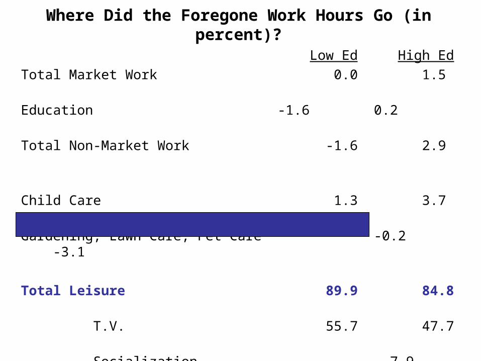
Where Did the Foregone Work Hours Go (in percent)?
Low Ed High Ed
Total Market Work 0.0 1.5
Education -1.6 0.2
Total Non-Market Work -1.6 2.9
Child Care 1.3 3.7
Gardening, Lawn Care, Pet Care -0.2 -3.1
Total Leisure 89.9 84.8
T.V. 55.7 47.7
Socialization 7.9 6.6
Sleeping 19.1 24.8
Other Entertainment/Hobbies 5.6 4.2
Own Medical Care 8.5 8.8
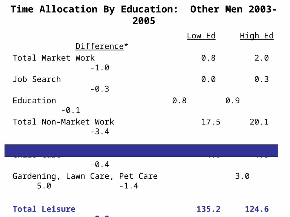
Time Allocation By Education: Other Men 2003-2005
Low Ed High Ed Difference*
Total Market Work 0.8 2.0 -1.0
Job Search 0.0 0.3 -0.3
Education 0.8 0.9 -0.1
Total Non-Market Work 17.5 20.1 -3.4
Child Care 4.0 4.5 -0.4
Gardening, Lawn Care, Pet Care 3.0 5.0 -1.4
Total Leisure 135.2 124.6 9.8
T.V. 32.9 24.6 8.5
Own Medical Care 1.4 2.3 -1.0
Care of Other Adults 2.2 2.5 0.0
Religious/Civic Activities 2.5 3.6 -0.8
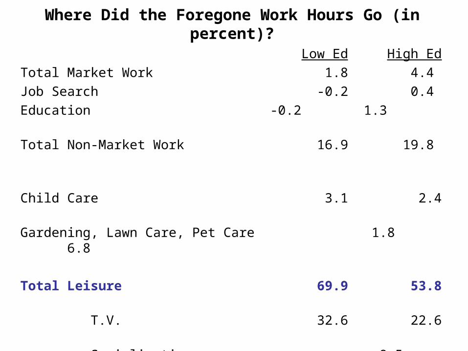
Where Did the Foregone Work Hours Go (in percent)?
Low Ed High Ed
Total Market Work 1.8 4.4
Job Search -0.2 0.4
Education -0.2 1.3
Total Non-Market Work 16.9 19.8
Child Care 3.1 2.4
Gardening, Lawn Care, Pet Care 1.8 6.8
Total Leisure 69.9 53.8
T.V. 32.6 22.6
Socialization 8.5 9.2
Sleeping 18.7 14.7
Other Entertainment/Hobbies 5.8 2.9

2003-2005 Cross Sectional Decomposition
• How much of the difference in leisure between high and low educated men in 2003-2005 is due to differences in job status?
Perform a Blinder-Oaxaca Decomposition:
Define Wjk = probability of being in job status k for educational attainment j
Xjk = hours per week of leisure for individual in job status k and educational attainment j.
Conditional Difference: 7.5 Hours Per Week
(WL – WH) XH (vectors): 2.4 Hours Per Week
WL(XL – XH) (vectors): 5.1 Hours Per Week
• Roughly 30% of difference in leisure in 2003-2005 between low and high educated men can be attributed to employment status differences.
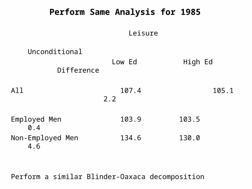
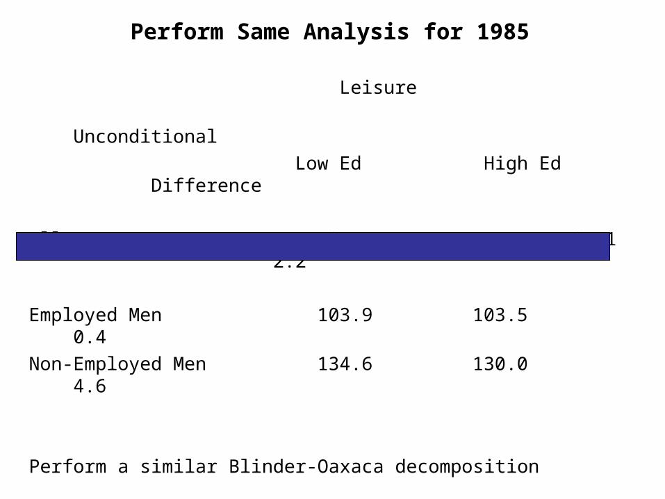
Perform Same Analysis for 1985
Leisure
Unconditional
Low Ed High Ed Difference
All 107.4 105.1 2.2
Employed Men 103.9 103.5 0.4
Non-Employed Men 134.6 130.0 4.6
Perform a similar Blinder-Oaxaca decomposition
• Roughly 60% of difference in leisure in 1985 between low and high educated men can be attributed to employment status differences.
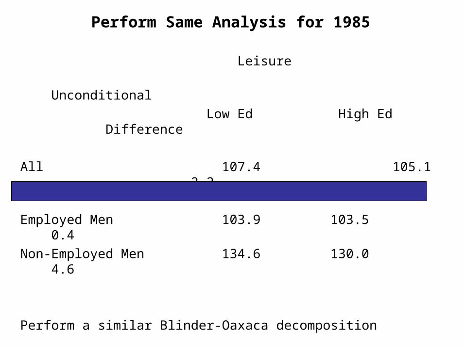
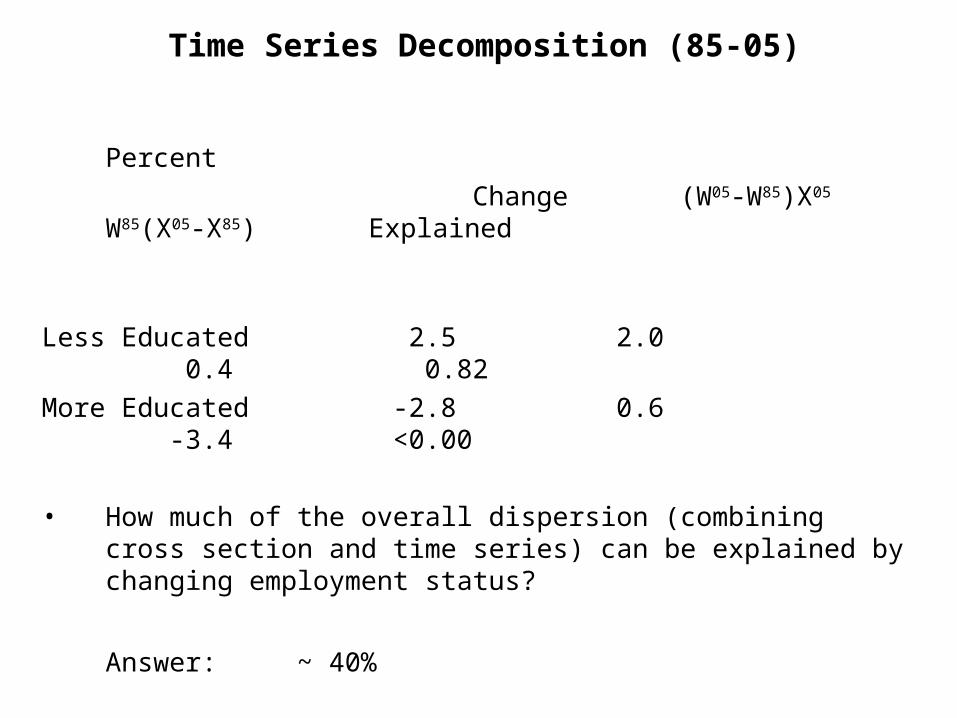
Time Series Decomposition (85-05)
Percent
Change (W05-W85)X05 W85(X05-X85) Explained
Less Educated 2.5 2.0 0.4 0.82
More Educated -2.8 0.6 -3.4<0.00
• How much of the overall dispersion (combining cross section and time series) can be explained by changing employment status?
Answer: ~ 40%
• Conclusion: If all non-employment is involuntary for low educated men, 60% of the documented leisure dispersion remains.
• Low educated men are still “choosing” to take more leisure than high educated men over last 25 years.
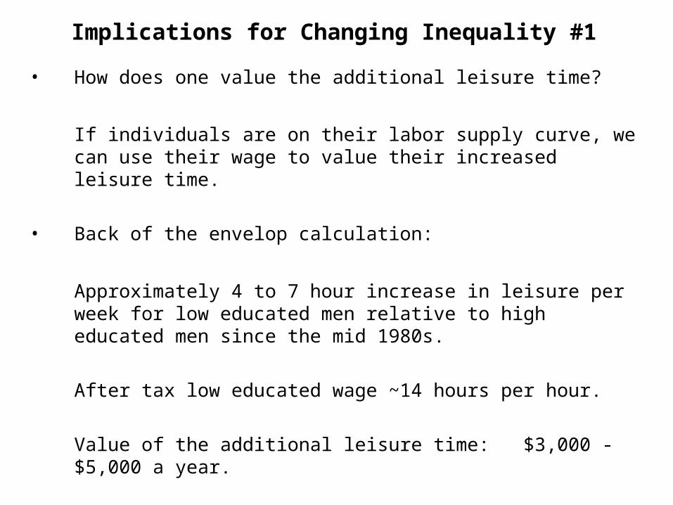
Implications for Changing Inequality #1
• How does one value the additional leisure time?
If individuals are on their labor supply curve, we can use their wage to value their increased leisure time.
• Back of the envelop calculation:
Approximately 4 to 7 hour increase in leisure per week for low educated men relative to high educated men since the mid 1980s.
After tax low educated wage ~14 hours per hour.
Value of the additional leisure time: $3,000 - $5,000 a year.
• Is this large?
Implications for Changing Inequality #2
• Provides a caution for interpreting measures of consumption inequality.
Time can be allocated to “home production” which can cause expenditure to diverge from true consumption.
Examples: Shopping intensity
Take advantage of time dependent discounts
Cooking meals
Do their own home production
• The unemployed do allocate more time to home production/shopping than their employed counterparts.
• Changes in employment propensities over time can be expected to change the mix of market expenditures and time that enter the commodity production function. (Aguiar and Hurst 2005, 2007a, 2007b)
Broader Implications
• Why do low educated men choose higher leisure relative to higher educated men?
1) Do wages differences cause the leisure differences?
– Substitution effects are important?
2) Or are preference differences driving the leisure differences? There are stark differences in behavior among the non-employed.
- Perhaps those with a taste for leisure are sorting are the ones
sorting into the low educated category.
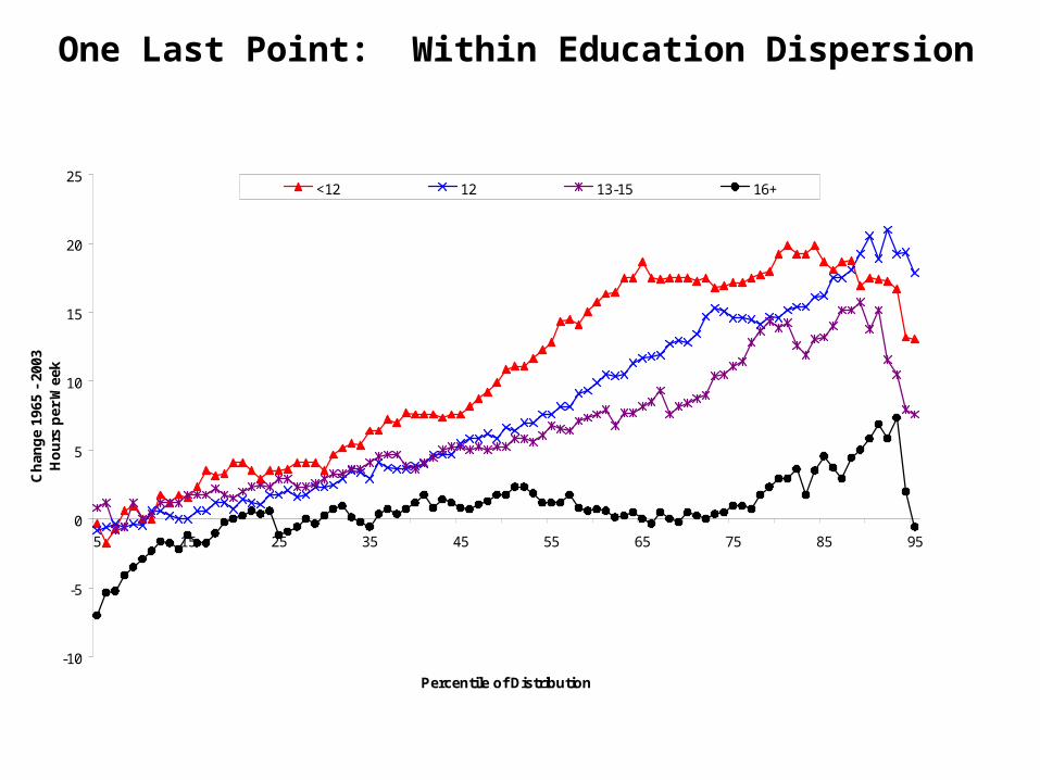
One Last Point: Within Education Dispersion
-10
-5
0
5
10
15
20
25
5 15 25 35 45 55 65 75 85 95
Percentile of Distribution
Ch
ang
e 19
65 -
200
3H
ou
rs p
er W
eek
<12 12 13-15 16+
Conclusions (Update)
• The allocation of time has changed dramatically over the last 40 years.
• The allocation differed dramatically by educational attainment with low educated individuals experiencing larger “leisure” increases than high educated individuals.
• Only about 40% of the dispersion can be explained by involuntary non-employment.

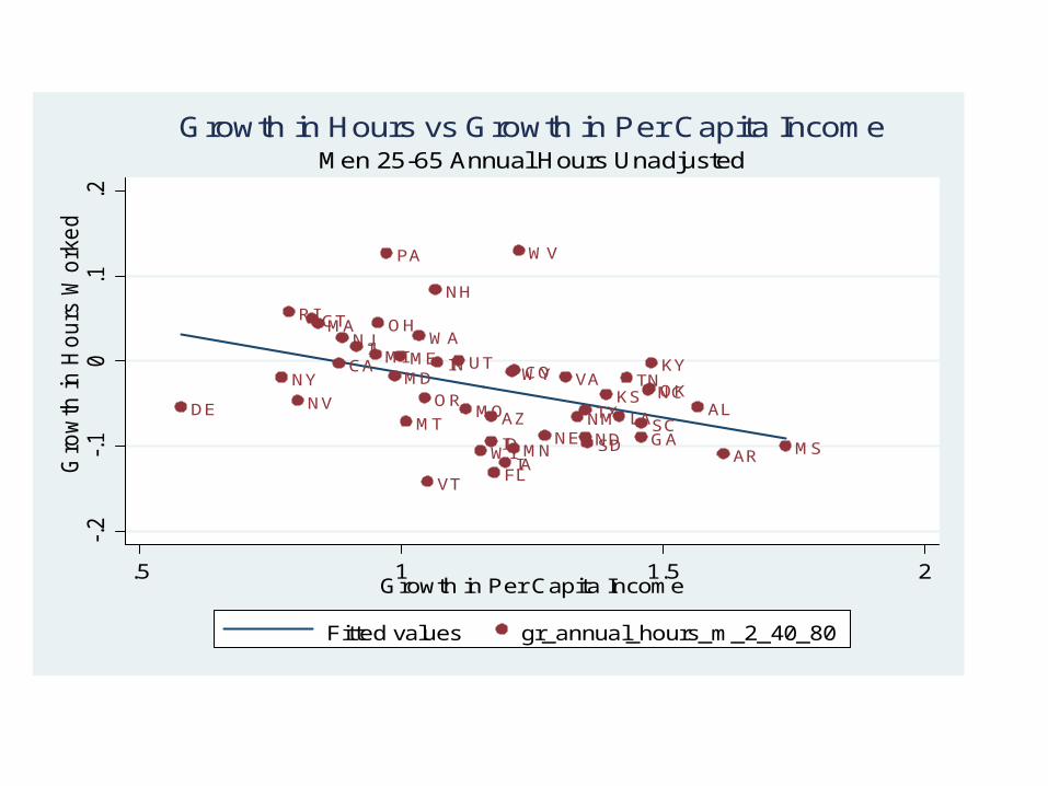
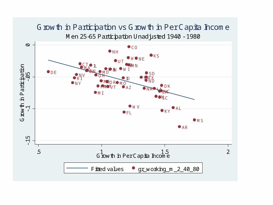
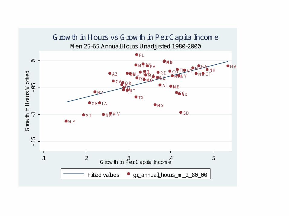
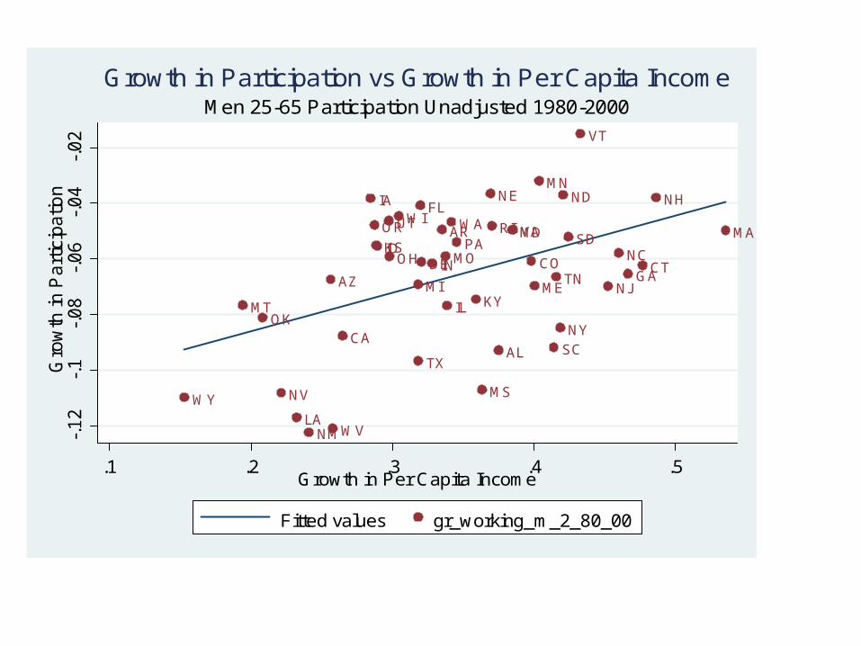
Part 3:Other Data I am Thinking About
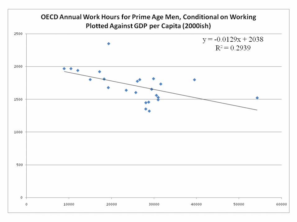
Do Income Effects Dominate Substitution Effects?
• I am not sure
ALAZ
AR
CA CO
CT
DE
FL
GAID
ILIN
IA
KS
KY
LA
MEMD
MA
MI
MN MS
MOMT
NE
NV
NH
NJ
NM
NYNC
ND
OH
OKOR
PA
RI
SCSD
TN
TX
UT
VT
VA
WA
WV
WI
WY
-.2
-.1
0.1
.2G
row
th in
Hours
Work
ed
.5 1 1.5 2Growth in Per Capita Income
Fitted values gr_annual_hours_m_2_40_80
Men 25-65 Annual Hours UnadjustedGrowth in Hours vs Growth in Per Capita Income
AL
AZ
AR
CA
CO
CT
DE
FL
GA
ID
ILIN
IA
KS
KY
LA
ME
MDMA
MI
MN
MS
MOMT
NE
NV
NH
NJ
NMNY
NC
NDOH
OKOR
PA
RI
SC
SD
TN
TX
UT
VT
VA
WA
WV
WI
WY
-.15
-.1
-.05
0G
row
th in
Pa
rtic
ipat
ion
.5 1 1.5 2Growth in Per Capita Income
Fitted values gr_working_m_2_40_80
Men 25-65 Participation Unadjusted 1940 - 1980Growth in Participation vs Growth in Per Capita Income
AL
AZ
AR
CA
CO CTDE
FL
GA
ID
ILIN
IAKS
KY
LA
ME
MDMAMI
MN
MS
MO
MT
NE
NV
NHNJ
NM
NY NC
ND
OH
OK
OR
PA
RI
SC
SD
TN
TX
UT
VT
VA
WA
WV
WI
WY
-.15
-.1
-.05
0G
row
th in
Hou
rs W
orke
d
.1 .2 .3 .4 .5Growth in Per Capita Income
Fitted values gr_annual_hours_m_2_80_00
Men 25-65 Annual Hours Unadjusted 1980-2000Growth in Hours vs Growth in Per Capita Income
AL
AZ
AR
CA
CO CTDE
FL
GA
ID
IL
IN
IA
KS
KY
LA
ME
MD MA
MI
MN
MS
MO
MT
NE
NV
NH
NJ
NM
NY
NC
ND
OH
OK
ORPA
RI
SC
SD
TN
TX
UT
VT
VAWA
WV
WI
WY
-.12
-.1
-.08
-.06
-.04
-.02
Gro
wth
in P
art
icip
atio
n
.1 .2 .3 .4 .5Growth in Per Capita Income
Fitted values gr_working_m_2_80_00
Men 25-65 Participation Unadjusted 1980-2000Growth in Participation vs Growth in Per Capita Income

Do Income or Substitution Effects Dominate onLabor Supply Decisions?
Part 4:Estimating Home Production Functions
Aguiar and Hurst (AER 2007)
85
Some Preliminaries
• Within most economic models, individual well being is usually measured as some function of consumption (c) and leisure (l) (i.e., U(c,l) )
• Empirically:
c is always measured as market expenditures (in dollars)
l is usually measured as time spent away from market work
• To the extent that non market activities are important (i.e., shopping and home production), the empirical measurements of c and l may not map directly into their theoretical counterparts.
86
An Example: Shopping
• Expenditure is price (p) * quantity (q) <<our measure of consumption>>
• Shopping is time intensive but it may affect prices paid (holding quantities constant)
• Given that time is an input into shopping, the opportunity cost of one’s time should determine how much an individual shops.
– Those whose time is less valuable should shop more and, all else equal, pay lower prices (holding quantities constant)
• A similar story could be told for home production
• By focusing on expenditure as sole measure of consumption, researchers will make false conclusions about individual well being.
– For example, declines in expenditure at the time of retirement
87
What We Do in This Paper
• Use new scanner data (on household grocery packaged goods) to document:
– Prices paid differs across individuals for the same good
– Price paid varies with proxies for cost of time.
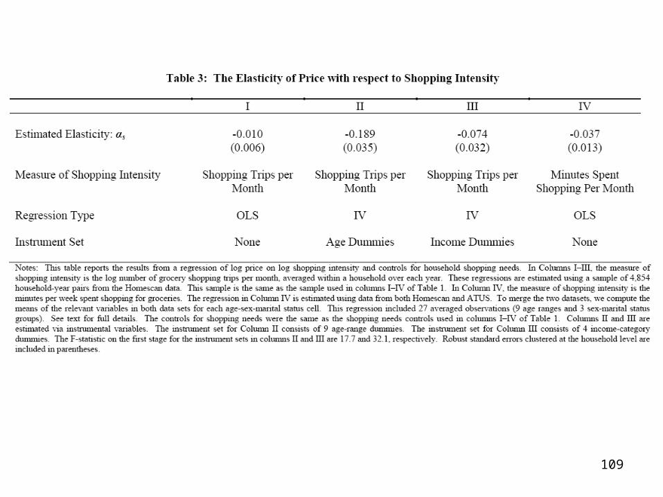
• Use this micro data to actually estimate household shopping functions which relate prices paid to shopping intensity.
– This shopping function will give us the implied opportunity cost of time for the shopper
• Given margin conditions, we can use the shopping function and time use data on home production to estimate the home production technology.
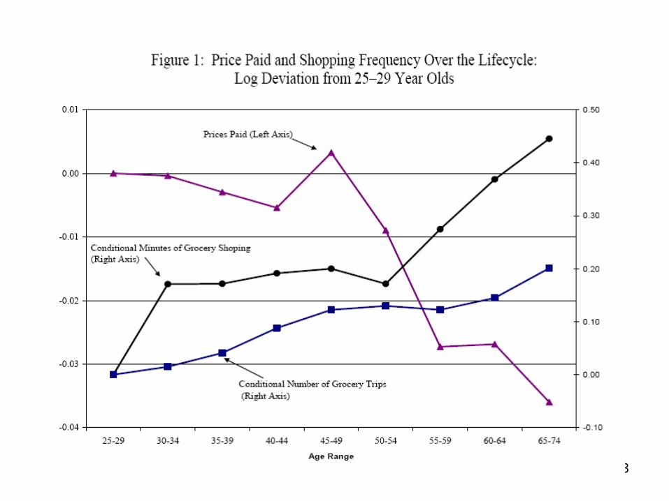
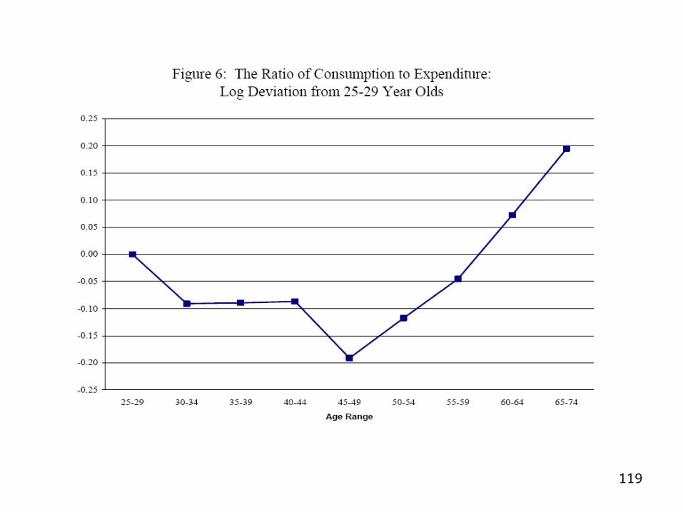
• Show empirically that the ratio of consumption to expenditure varies over the lifecycle

88
Scanner Data on Prices
• Note: In this data part of the paper, we will only be talking directly about food consumptions and expenditures (in model, we will extend the implications)
• Data is from AC Nielson HomeScan
– Panel of households
– Random sample within the MSA of households
• The survey is designed to be representative of the Denver metropolitan statistical area and summary demographics line up well with the 1994 PSID
– Coverage at several types of retail outlets

89
Scanner Data (continued)
• Each household is equipped with an electronic home scanning unit
• Each household member records every UPC-coded food purchase they make by scanning in the UPC code
• After each shopping trip, household records:
– What was purchased (i.e. scan in UPC code)
– Where purchase was made (specifically)
– Date of purchase
– Discounts/coupons (entered manually)
• AC Nielson collects the price data from all local shopping outlets.
• Data has decent demographics (income categories, household composition, employment status, sex, race, age of members, etc.). Collected annually.
90
• We have access to the Denver data for the years 1993-1995.
– Short panel
• Sample:
– 2,100 households (focus on age of shopper between 24 and 75) – 950,000 transactions – 40,000 household/month observations.
Sample
91
• Derive a price index using the scanner data
• Show some unconditional means of how this price index varies across differing income and demographic groups
• Think about measurement issues relating to our estimate of the price index
• Goal is to get estimate shopping and home production functions that I could import into our model
How am I going to Use the Data
92
Potential Measurement Issue 1: Underreporting
• Average monthly expenditure in the data set: $176/month (1993 dollars)
• Average total food “at home” in the PSID for similarly defined sample (1993 dollars) is $320 (55% coverage rate in the HomeScan Data)
• Differences between the coverage due to:
– Omission of certain grocery expenditures due to lack of UPC code (some meat, diary, fresh fruit and vegetables).
– Omission of expenditures due to household self-scanning.
• Explore underreporting by different age/education/year cells (forming a ratio by comparing homescan data to PSID). The gap does not vary with age – however, it does vary with education levels (only 42% of expenditures for high educated vs 55% for low educated).
• Underreporting not a problem for our analysis if random.
93
Potential Measurement Issue 2: Attrition
• Cannot observe on the extensive margin (homescan only releases data for households who participated consistently over the sample)
• Can observe attrition on intensive margin
– Compare average expenditures in Homescan between 1993, 1994, and 1995
– first quarter of 1994 had 1% less expenditures than first quarter of 1993
– first quarter of 1995 had 5% less expenditures than first quarter of 1993
• No difference in expenditure declines by age or education
• For completeness, we redid our whole analysis only including 1993 – no differences found
94
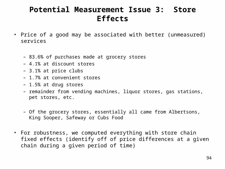
Potential Measurement Issue 3: Store Effects
• Price of a good may be associated with better (unmeasured) services
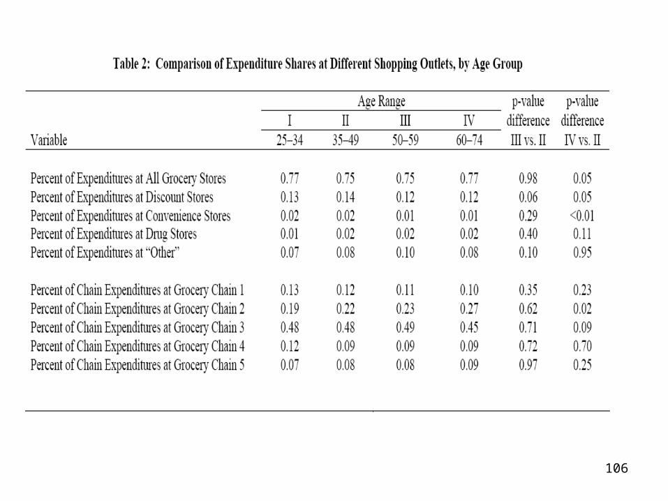
– 83.6% of purchases made at grocery stores
– 4.1% at discount stores
– 3.1% at price clubs
– 1.7% at convenient stores
– 1.5% at drug stores
– remainder from vending machines, liquor stores, gas stations, pet stores, etc.
– Of the grocery stores, essentially all came from Albertsons, King Sooper, Safeway or Cubs Food
• For robustness, we computed everything with store chain fixed effects (identify off of price differences at a given chain during a given period of time)
95
Aggregation over Prices
• We want a summary of the price a household pays
– Relate to cost of time
• Households buy many goods and basket varies over time
– Look at one popular good (milk)
– Define an index that answers: For its particular basket of goods, does this household pay more or less than other households?
96
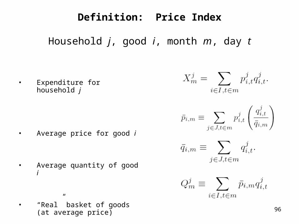
Definition: Price Index
Household j, good i, month m, day t
• Expenditure for household j
• Average price for good i
• Average quantity of good i
• “Real” basket of goods (at average price)
97
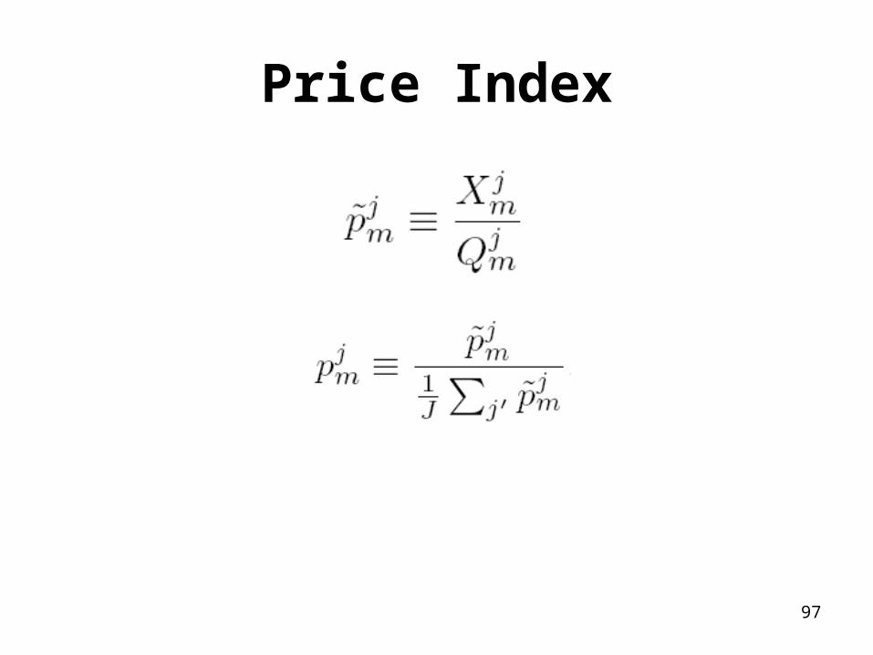
Price Index
98
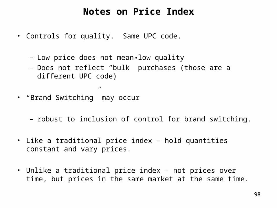
Notes on Price Index
• Controls for quality. Same UPC code.
– Low price does not mean low quality
– Does not reflect “bulk” purchases (those are a different UPC code)
• “Brand Switching” may occur
– robust to inclusion of control for brand switching.
• Like a traditional price index – hold quantities constant and vary prices.
• Unlike a traditional price index – not prices over time, but prices in the same market at the same time.
99
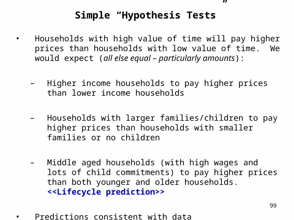
Simple “Hypothesis Tests”
• Households with high value of time will pay higher prices than households with low value of time. We would expect (all else equal – particularly amounts):
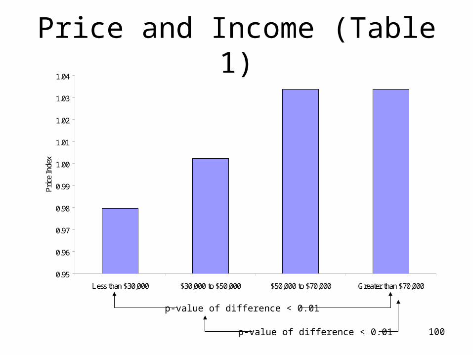
– Higher income households to pay higher prices than lower income households
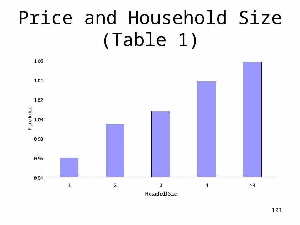
– Households with larger families/children to pay higher prices than households with smaller families or no children
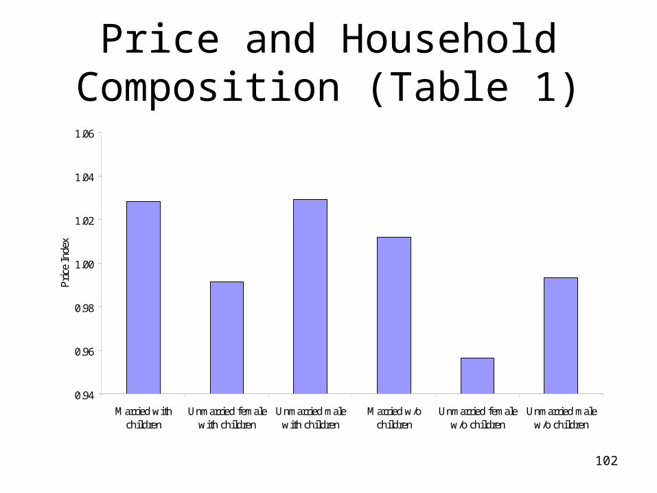
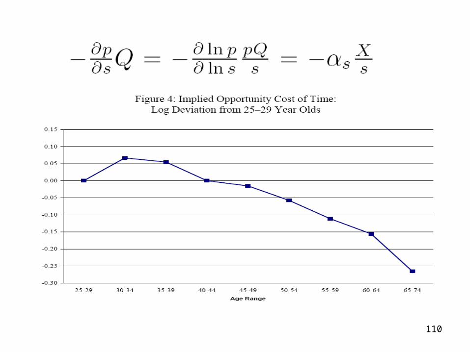
– Middle aged households (with high wages and lots of child commitments) to pay higher prices than both younger and older households. <<Lifecycle prediction>>
• Predictions consistent with data
100
Price and Income (Table 1)
0.95
0.96
0.97
0.98
0.99
1.00
1.01
1.02
1.03
1.04
Less than $30,000 $30,000 to $50,000 $50,000 to $70,000 Greater than $70,000
Pri
ce I
ndex
p-value of difference < 0.01
p-value of difference < 0.01
101
Price and Household Size (Table 1)
0.94
0.96
0.98
1.00
1.02
1.04
1.06
1 2 3 4 >4
Hosuehold Size
Pri
ce I
ndex
102
Price and Household Composition (Table 1)
0.94
0.96
0.98
1.00
1.02
1.04
1.06
Married withchildren
Unmarried femalewith children
Unmarried malewith children
Married w/ochildren
Unmarried femalew/o children
Unmarried malew/o children
Pri
ce I
ndex
103
104
105
106
107
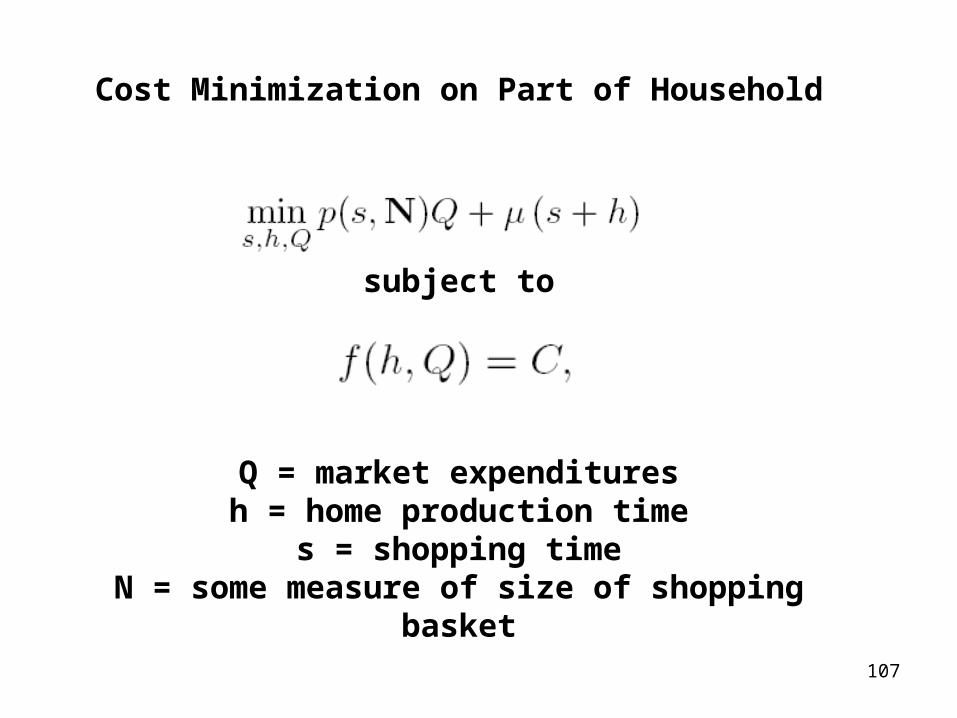
Cost Minimization on Part of Household
subject to
Q = market expendituresh = home production time
s = shopping timeN = some measure of size of shopping basket
108
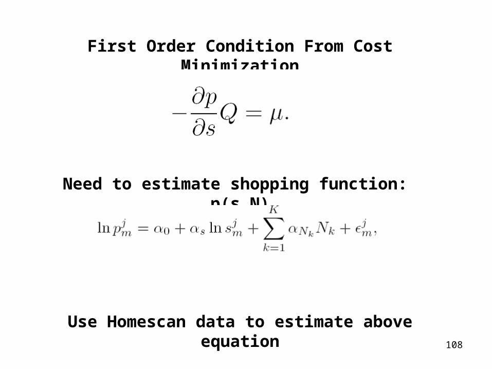
First Order Condition From Cost Minimization
Need to estimate shopping function: p(s,N)
Use Homescan data to estimate above equation
109
110
111
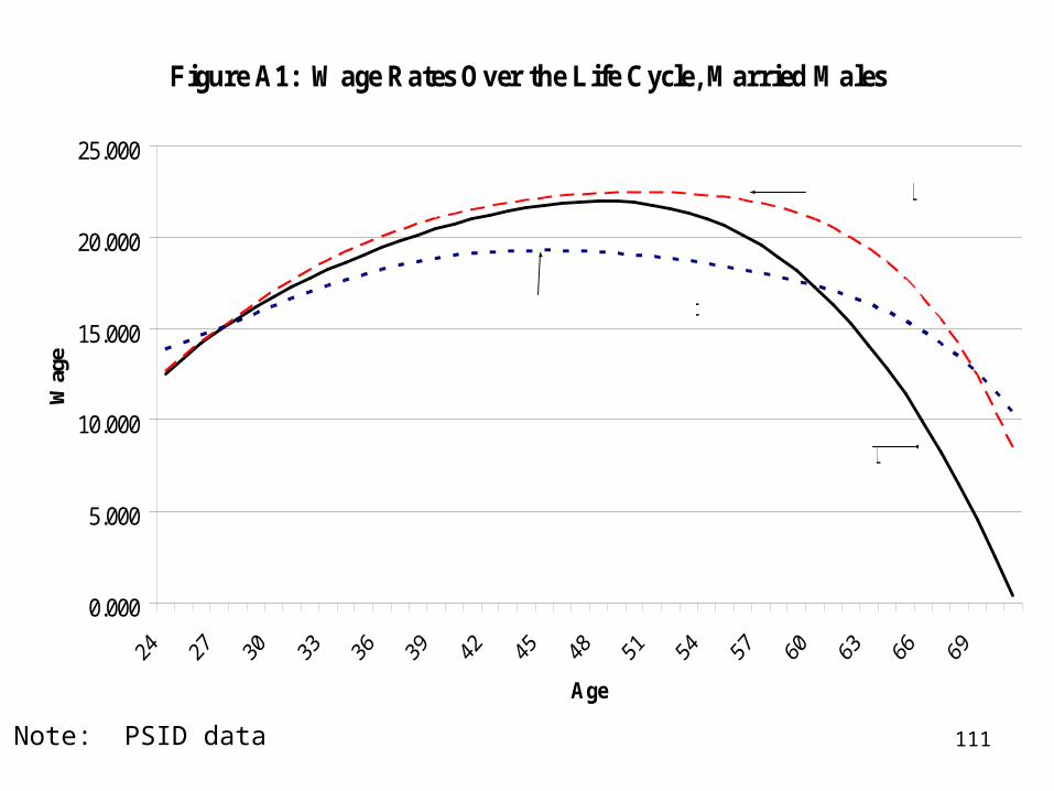
Figure A1: Wage Rates Over the Life Cycle, Married Males
0.000
5.000
10.000
15.000
20.000
25.000
Age
Wag
e
Conditional/Fixed Effect
Unconditional
Conditional
Note: PSID data
112
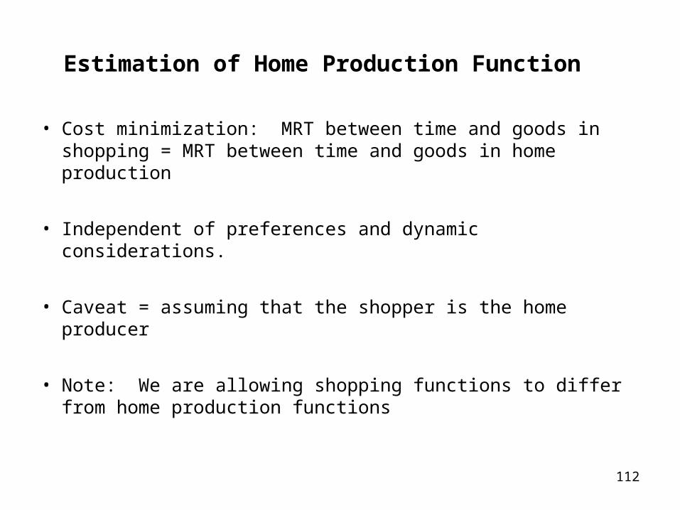
Estimation of Home Production Function
• Cost minimization: MRT between time and goods in shopping = MRT between time and goods in home production
• Independent of preferences and dynamic considerations.
• Caveat = assuming that the shopper is the home producer
• Note: We are allowing shopping functions to differ from home production functions
113
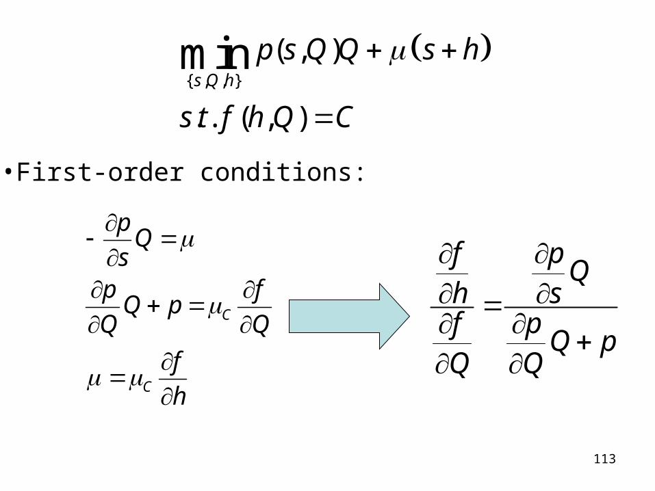
{ , , }
( , )
. . ( , )
mins Q h
p s Q Q s h
s t f h Q C
C
C
pQ
sp f
Q pQ Q
f
h
•First-order conditions:
f pQ
h sf p
Q pQ Q
114
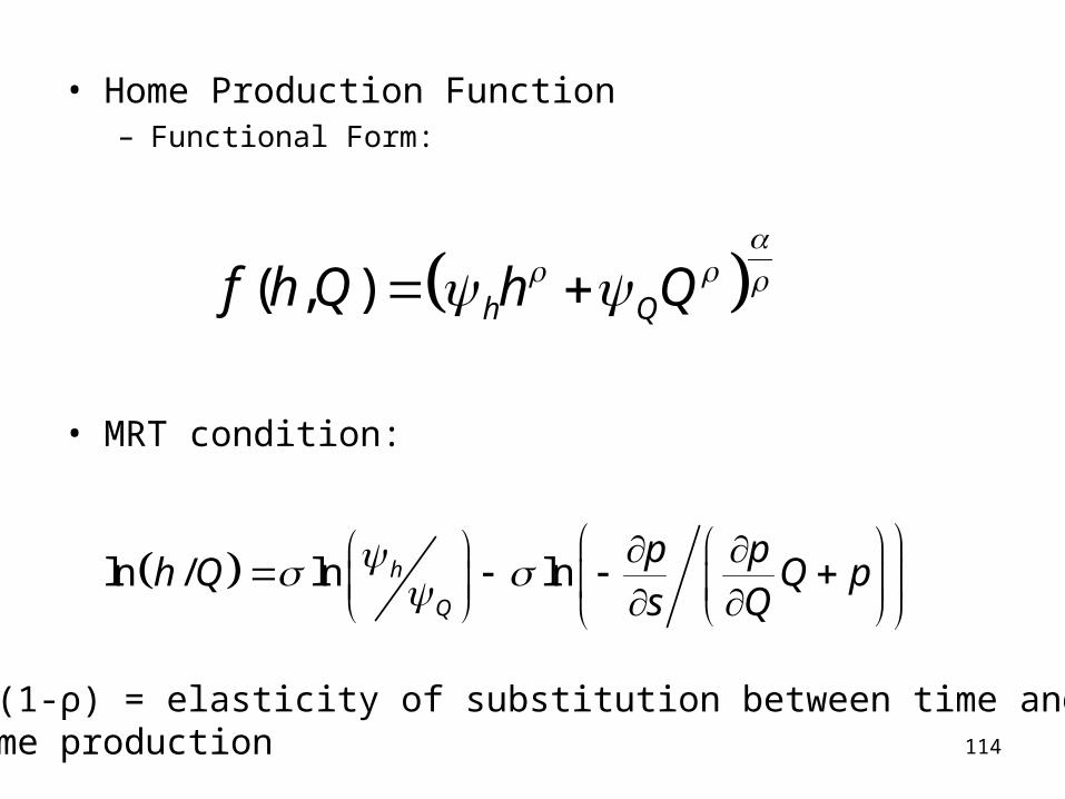
• Home Production Function– Functional Form:
• MRT condition:
( , ) h Qf h Q h Q
ln / ln lnh
Q
p ph Q Q p
s Q
• σ= 1/(1-ρ) = elasticity of substitution between time and goodsin home production

115
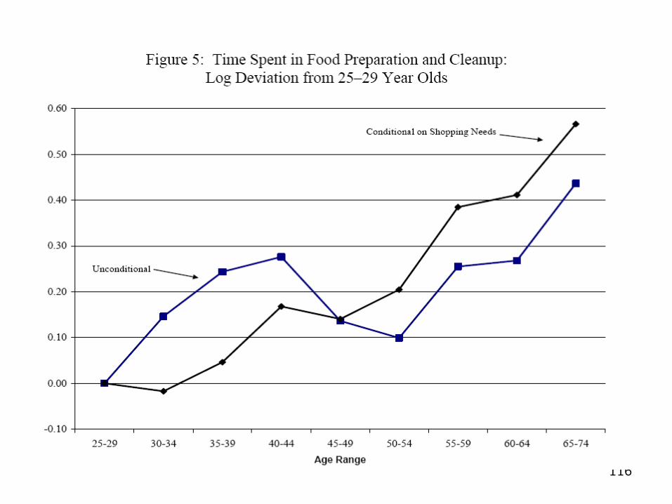
• RHS variable can be constructed from shopping data.
• No measure of h in scanner data set
– Merge in from ATUS using cells based on
– 92 separate cells represented in data
• Run “between effects” regression over cells
116
117
118
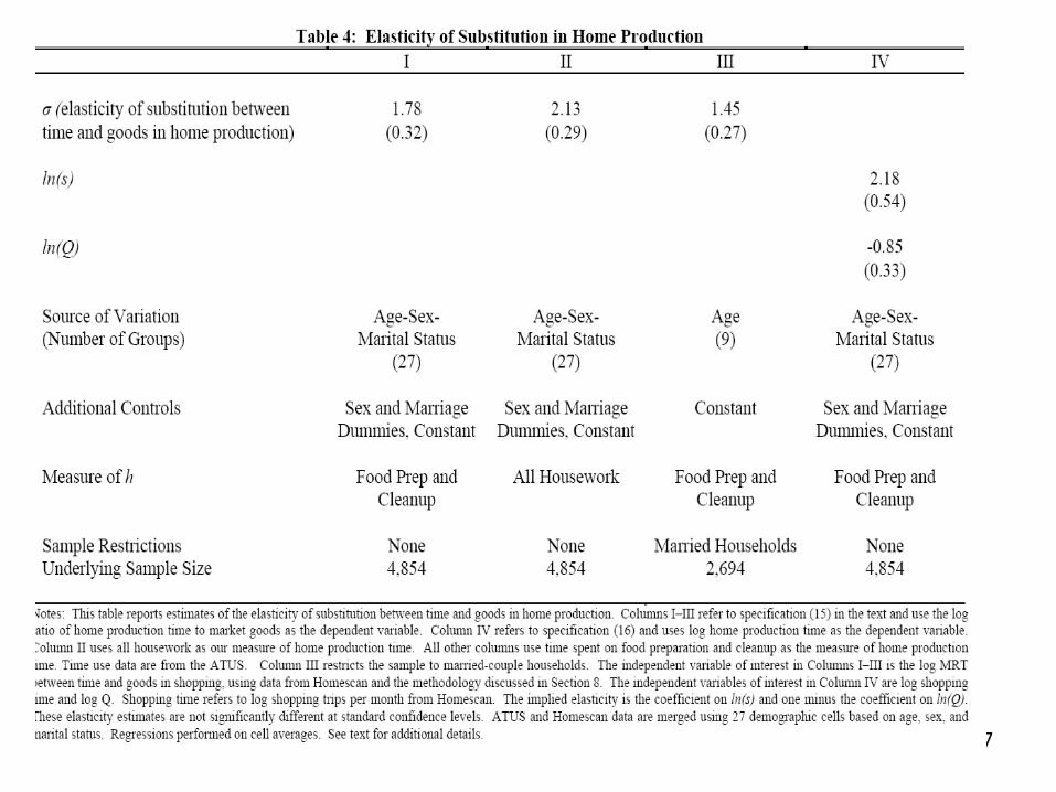
• We estimate an elasticity of substitution between time and goods in home production between 1.5 and 2.1.
– Less aggregation leads to lower estimates
• With estimated home production parameters, can estimate actual consumption given observed inputs.
– Consumption/Expenditure varies over lifecycle
– Even if consumption and leisure are separable in utility, need to be careful in interpreting lifecycle expenditure.
119
120
Conclusions (Need To Update)
• Fairly large elasticities between time and money due to shopping and home production.
• We find that households can and do alter the relationship between expenditures and consumption by varying time inputs.
• Household time use, prices, and expenditures vary in a way that is consistent with standard economic principles and the lifecycle profile of the relative price of time.
• Supports growing emphasis on importance of non-market sector in understanding household’s interaction in market
– Expenditures: “Hump” in household expenditures – particularly decline after middle age – consistent with forward-looking, patient agents.
– Labor supply: Stable market hours over last 40 years masks dramatic changes in time spent in home production and leisure.