LABOR SUPPLY

I. Consumer theoryII. Labor supply by individualsIII. What happens when

wages changeIV. Elasticity of labor supply

I. CONSUMER THEORY

Basis for theory of labor supply

SIMPLIFYING ASSUMPTIONSTwo Good WorldIndividuals express preferences

for 1 good in terms of what they will give up of another

Want more of everything

CONSTRAINED MAXIMIZATION PROBLEM: What one wants

Individual PreferencesExpressed in terms of Utility

derived from good or service (No $$ yet)

Negative slope (How much will you give up?)

Subject to diminishing returnsDifferent curves for different

people

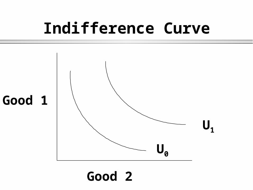
Indifference Curve

Good 2

Good 1

U0

U1

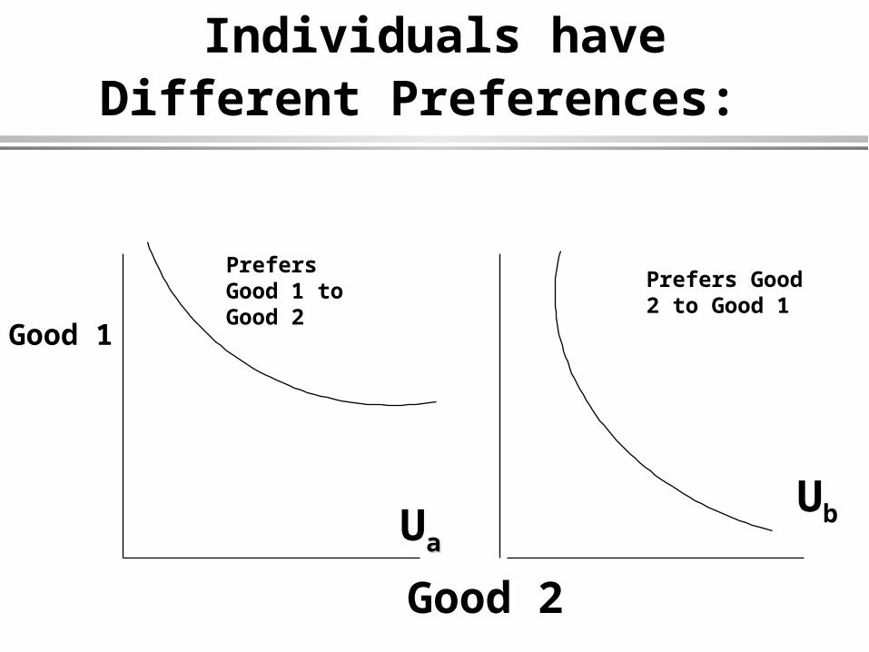
Individuals have Different Preferences:

Good 2

Good 1

Uaa

Ub

Prefers Good 1 to Good 2

Prefers Good 2 to Good 1

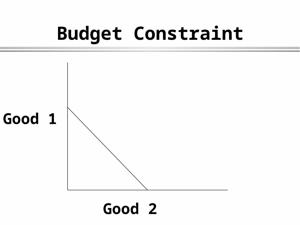
CONSTRAINED MAXIMIZATION: THE CONSTRAINT

Budget ConstraintExpressed in terms of relative

prices (price of good 1 and price of good 2)

Opportunity Cost: How much you would have to give up of good 1 to be able to afford more of good 2

Negative slopeSlope of line = relative price of 2 goods

Budget Constraint

Good 2

Good 1

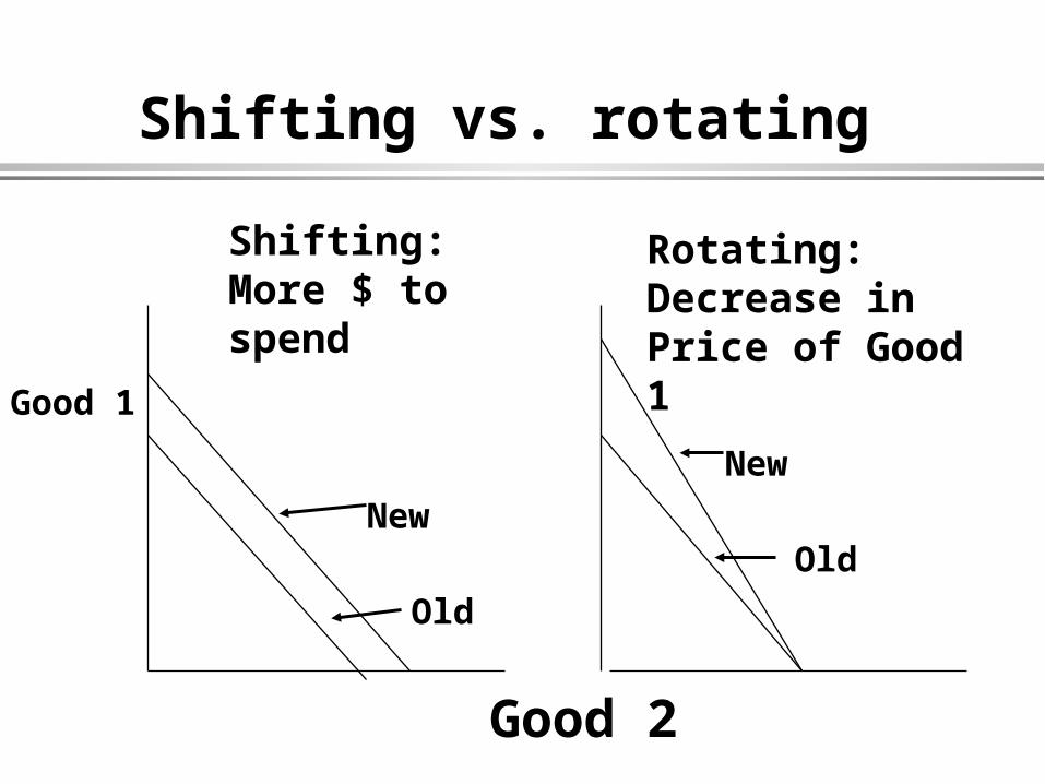
Shifting vs. rotating budget constraint

SHIFTING Occurs when

have move income to spend

Slope of line does not change

ROTATING Occurs when

relative prices change E.g., When good

one becomes more or less expensive relative to good two

Slope of line does change

Shifting vs. rotating

Good 2

Good 1

Shifting: More $ to spend

Rotating: Decrease in Price of Good 1

Old

New

New

Old

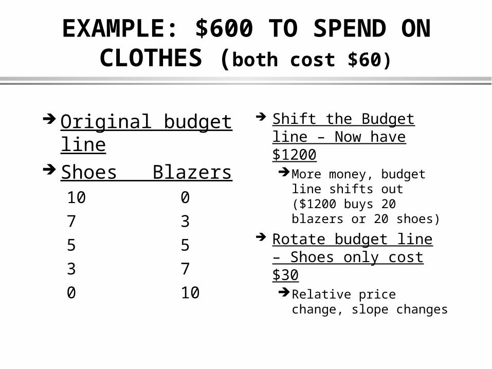
EXAMPLE: $600 TO SPEND ON CLOTHES (both cost $60)

Original budget line

Shoes Blazers10 07 35 53 70 10

Shift the Budget line – Now have $1200More money, budget

line shifts out ($1200 buys 20 blazers or 20 shoes)

Rotate budget line – Shoes only cost $30Relative price change,

slope changes

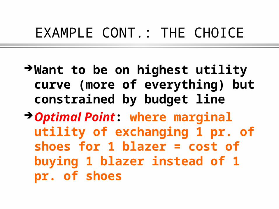
EXAMPLE CONT.: THE CHOICE

Want to be on highest utility curve (more of everything) but constrained by budget line

Optimal Point: where marginal utility of exchanging 1 pr. of shoes for 1 blazer = cost of buying 1 blazer instead of 1 pr. of shoes

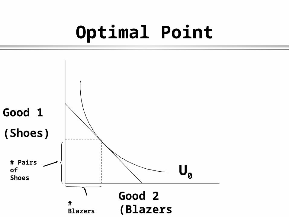
Optimal Point

Good 2 (Blazers)

Good 1

(Shoes)

U0

# Pairs of Shoes

# Blazers

II. LABOR SUPPLY DECISION

Applying Consumer Theory to Labor Supply

Two Goods LeisureAll other goods & services

(purchased with $)Consumer/worker deciding how

much to consume of each

INDIVIDUAL PREFERENCES

Hours of work: U=U(X,L)Depends on Demand for Leisure

How many goods will you give up to get more leisure?

Hours of Work = (Discretion Time) - Leisure

Diminishing Marginal UtilityFamily of CurvesDifferent Shapes for different people

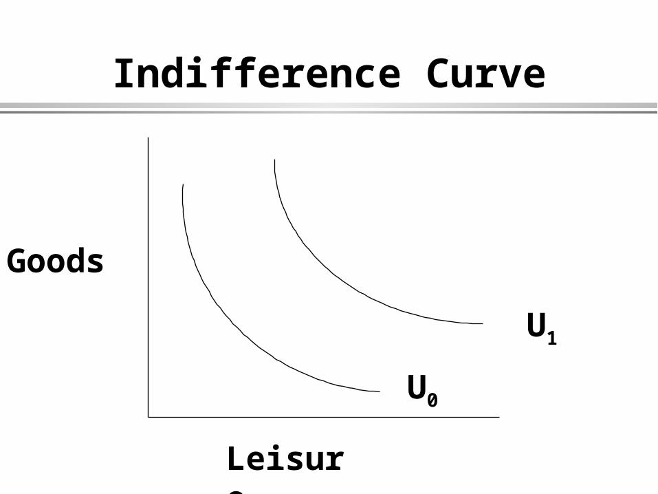
Indifference Curve

Leisure

Goods

U0

U1

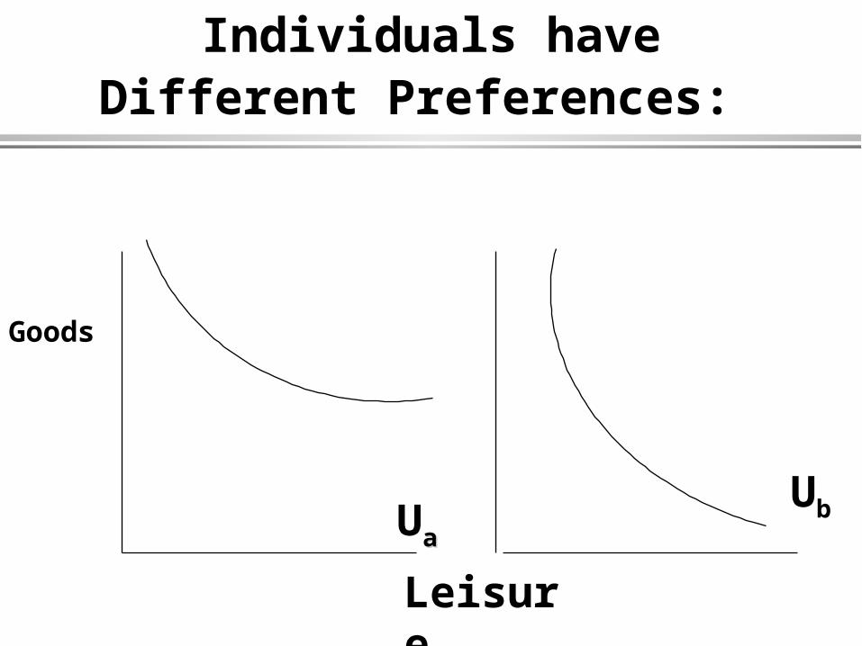
Individuals have Different Preferences:

Leisure

Goods

Uaa

Ub

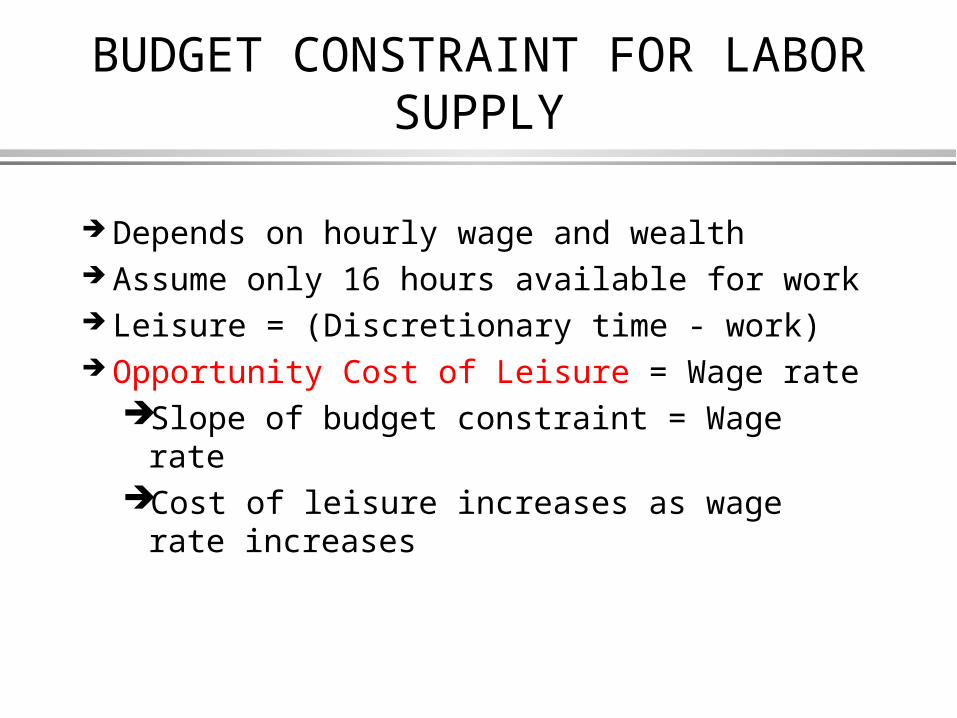
BUDGET CONSTRAINT FOR LABOR SUPPLY

Depends on hourly wage and wealth Assume only 16 hours available for work Leisure = (Discretionary time - work) Opportunity Cost of Leisure = Wage rate

Slope of budget constraint = Wage rate

Cost of leisure increases as wage rate increases

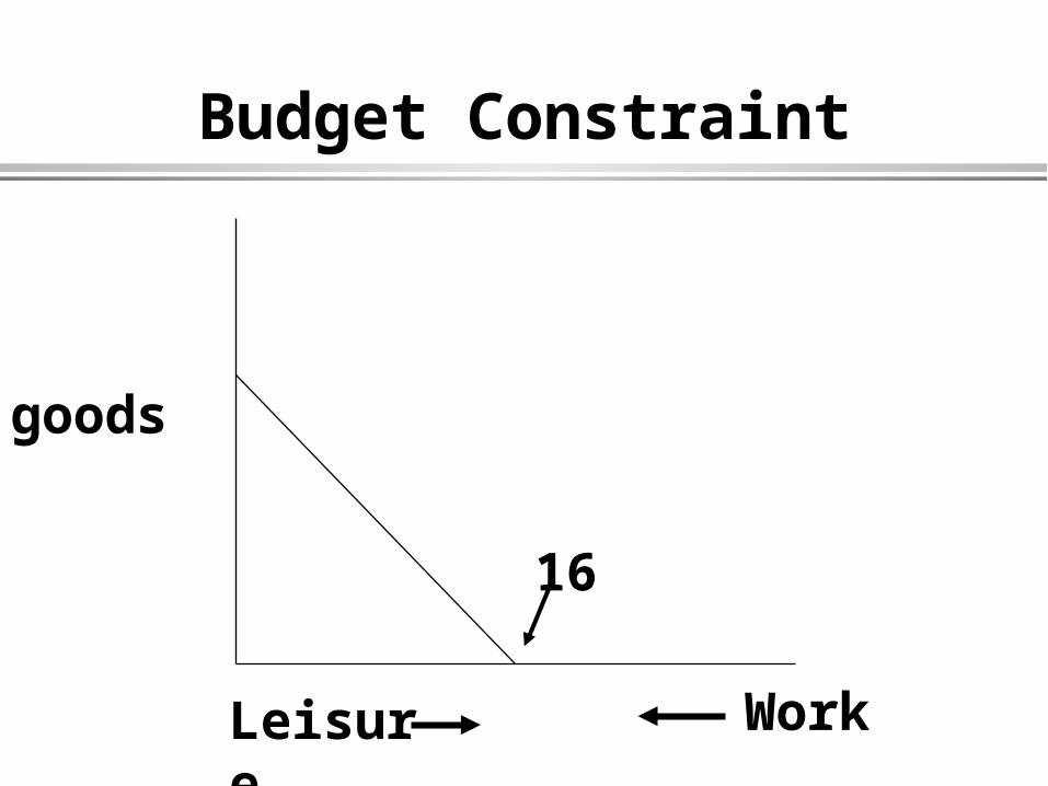
Budget Constraint

Leisure

goods

Work

16

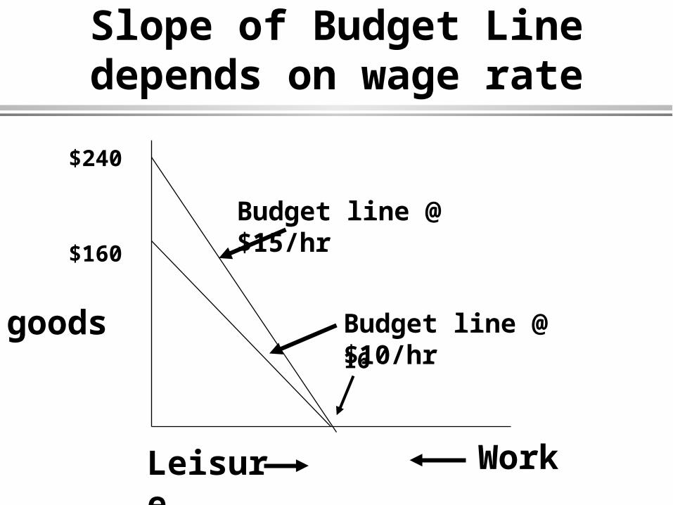
Slope of Budget Line depends on wage rate

Leisure

goods

Work

16

$160

Budget line @ $10/hr

$240

Budget line @ $15/hr

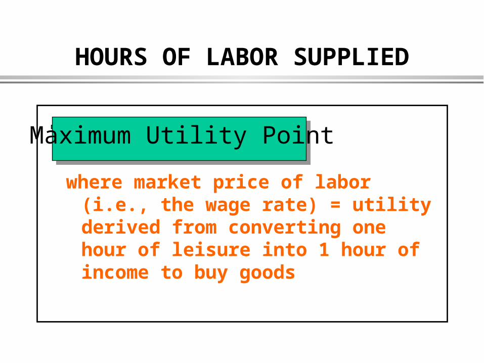
HOURS OF LABOR SUPPLIED

where market price of labor (i.e., the wage rate) = utility derived from converting one hour of leisure into 1 hour of income to buy goods

Maximum Utility Point

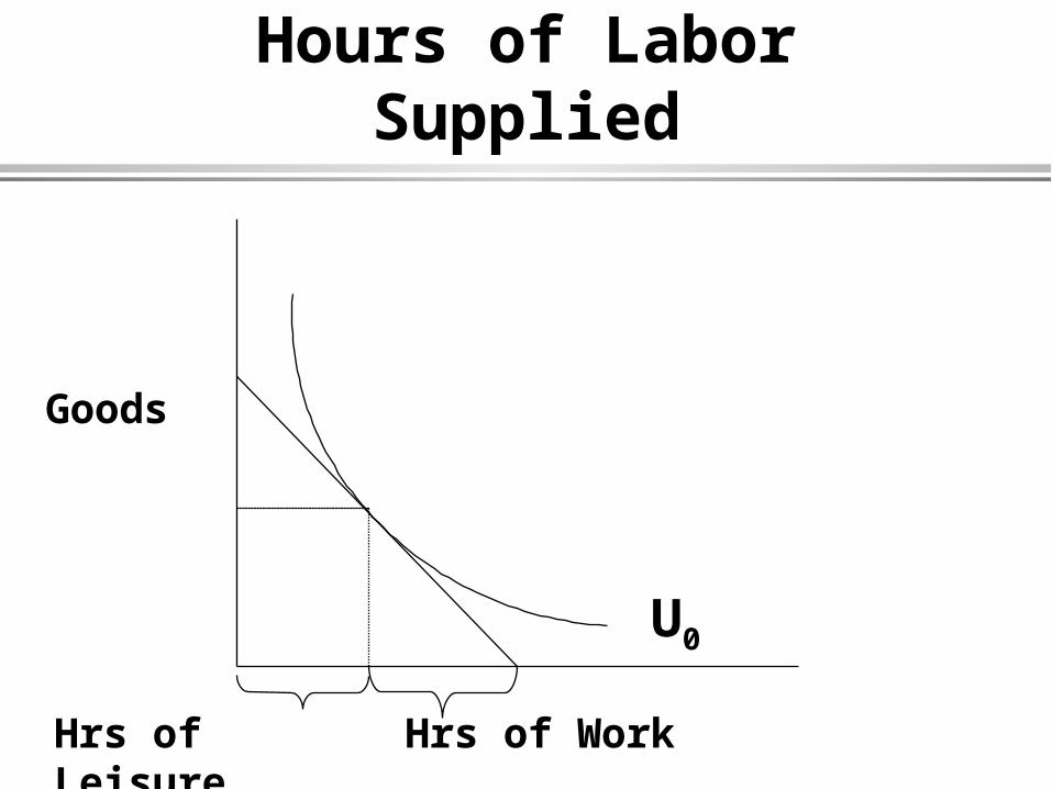
Hours of Labor Supplied

Hrs of Work

Goods

U0

Hrs of Leisure

Summary

Factors determining individual supply of labor Preferences for leisure versus goods

& services How much money one can earn in

the labor market How much wealth one has

III. EFFECT OF CHANGING WAGE RATE: 2 EFFECTS

1.SUBSTITUTION EFFECTResults from changing wage rateChange in wage rate = Change in

price of leisureWage Increase --> Increase price

of leisure --> Reduced demand for leisure --> Increased hours of work

Budget line rotates

EFFECT OF CHANGING WAGE RATE, CONT.

2. INCOME EFFECTWages increase wealthIncrease in wealth allows greater

consumption of “normal goods”Budget line shifts, no change in

slope BOTH EFFECTS OCCUR WITH WAGE

CHANGE2 Effects operate in opposite

directions

IV. ELASTICITY OF LABOR SUPPLY

Definition: % change qty. supplied/% change wages

Indicator of economic powerWage increase: the more inelastic the supply

of labor, the more powerful the workforceWage decrease: the more inelastic the supply

of labor, the less powerful the workforce

Supply of Labor more elastic:

In response to a wage increase: ·  Fewer barriers to entry (if raise wage): Skill,

education, and/or training time required to do the job, unions, internal labor market, certifications, etc.

·  The lower one’s preference for leisure ·  The lower one’s wealth In response to wage decrease: ·  The more employment alternatives elsewhere in the

market The greater one’s wealth ·  The greater one's preference for leisure

LABOR SUPPLY IN CONTEXT OF HOME LIFE

I. Theory of Household ProductionII. Supply by Multiple Members of the Household

I. THEORY OF HOUSEHOLD PRODUCTION: Household as “little factory”

Basic Premise: Individuals productive in two places, at home and in the market

Home Production Function: Goods can be purchased in the market or

produced at home Diminishing marginal productivity Differing productivity across individuals

HOME PRODUCTION AS PART OF BUDGET CONSTRAINT

TWO BUDGET CONSTRAINTS MONEY CONSTRAINT: Rate at

which can convert work hours to money (put with wealth) to buy goods & services

HOME CONSTRAINT: Rate at which can convert hours at home into goods & services

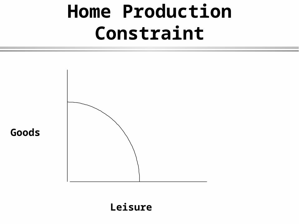
Home Production Constraint

Leisure

Goods

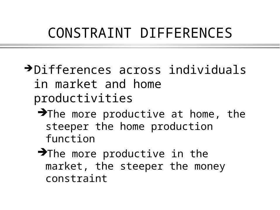
CONSTRAINT DIFFERENCES

Differences across individuals in market and home productivitiesThe more productive at home, the

steeper the home production functionThe more productive in the market,

the steeper the money constraint

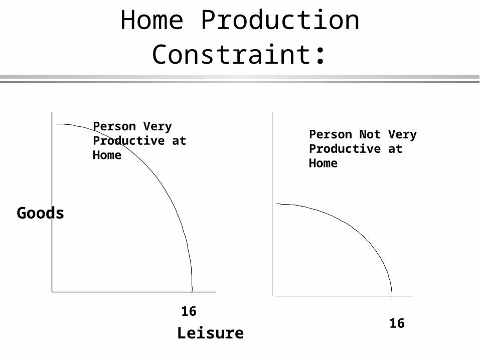
Home Production Constraint:

Leisure

Goods

Person Very Productive at Home

Person Not Very Productive at Home

1616

LABOR SUPPLY ALLOWING FOR HOME PRODUCTION

What is best mix of home-produced and market produced goods and services?

Maximize Utility = U(X,L), where X = Xh + Xm subj. to 2 budget constraints

Placement of curve Shape of curve shows trade-off b/n

purchased & home-produced goods Greater mkt. productivity -> greater

wage -> less home production

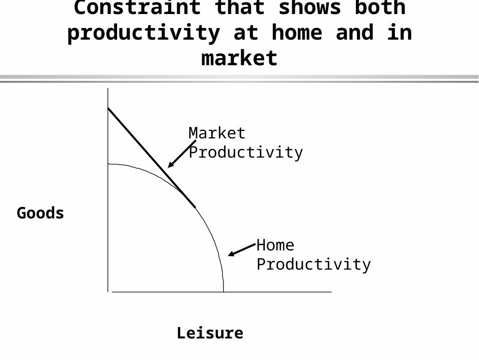
Constraint that shows both productivity at home and in

market

Leisure

Goods

Home Productivity

Market Productivity

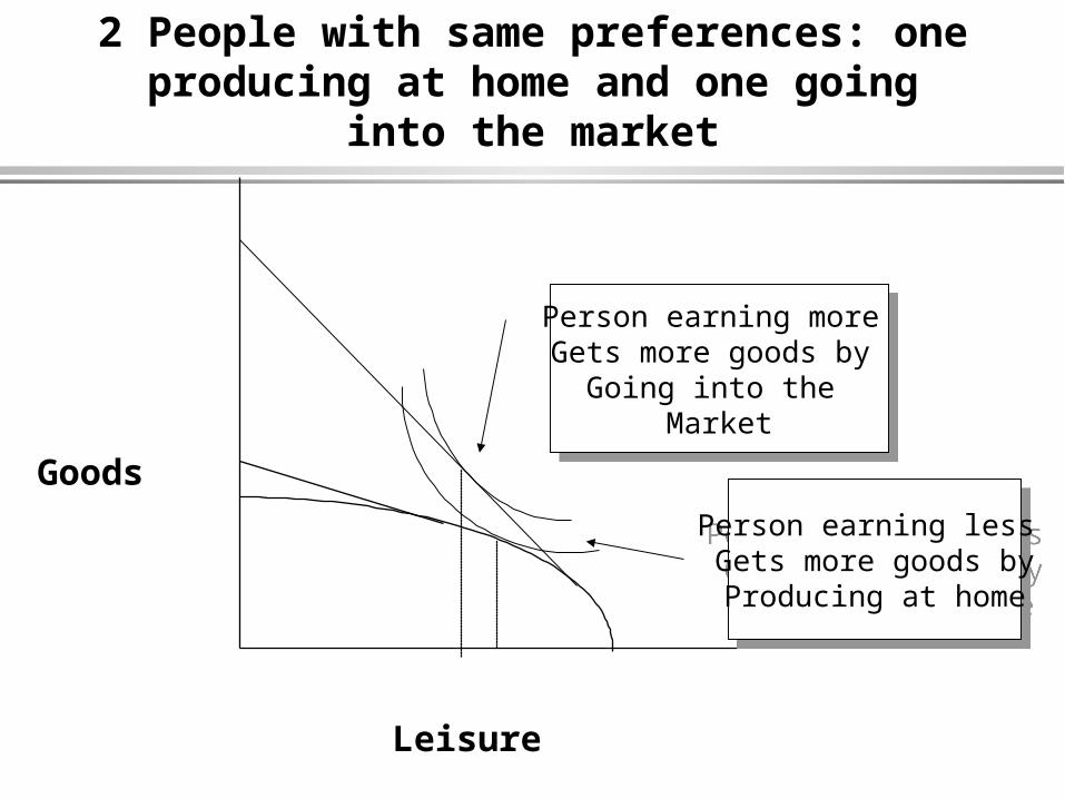
2 People with same preferences: one producing at home and one going

into the market

Leisure

Goods

Person earning more Gets more goods by

Going into the Market

Person earning more Gets more goods by

Going into the Market

Person earning less Gets more goods byProducing at home

Person earning less Gets more goods byProducing at home

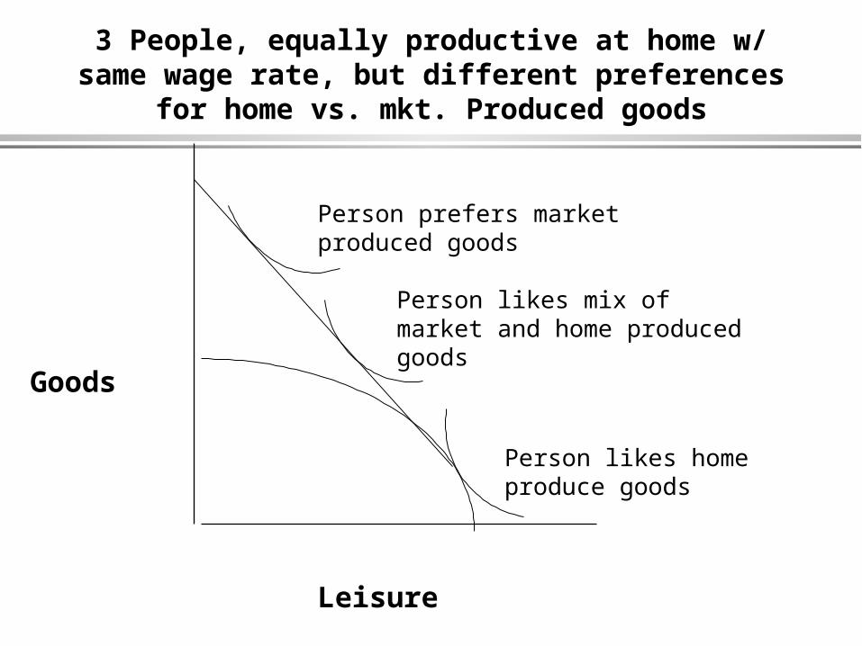
3 People, equally productive at home w/ same wage rate, but different preferences

for home vs. mkt. Produced goods

Leisure

Goods

Person prefers market produced goods

Person likes mix of market and home produced goods

Person likes home produce goods

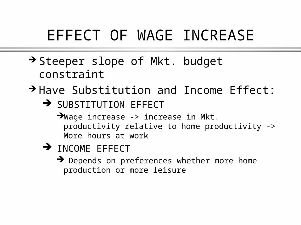
EFFECT OF WAGE INCREASE

Steeper slope of Mkt. budget constraint Have Substitution and Income Effect:

SUBSTITUTION EFFECTWage increase -> increase in Mkt. productivity

relative to home productivity -> More hours at work

INCOME EFFECT Depends on preferences whether more home

production or more leisure

SUMMARY

People differ in preferences for home & market produced goods

People differ in home productivity When wages are raised, some

people may work less

II. JOINT HOUSEHOLD LABOR SUPPLY DECISIONS

AssumptionsDecision-making unit: HH rather than

individual2 Potential earners

Point: Individuals make labor supply decisions based on household income and household preferences

HOUSEHOLD LABOR SUPPLY

Interdependent labor supply decisions Factors in Decision:

1) HH Preferences (mkt. goods, home goods, leisure)

2) Relative productivity at home & in marketInterdependent ProductivitiesProductivity of one spouse depends on other’s

supply to marketRecall diminishing marginal productivity of home

production

HH LABOR SUPPLY, CONT.

Decision Rule: if 1 hr. of work in mkt. by either person increases utility more than hr. of home work, will go into mkt.

Cross-elasticity of substitution: % Change Hi/ % Change Wj < > 0If > 0, couple are complementsIf < 0, couple is substitutes

Summary

Factors individuals take into account when making labor supply decision:Their earnings/wage rateTheir productivity at homeTheir wealthTheir preferences for market goods, home

produced goods and leisure These change with people’s life

circumstance.