mf620 1/2007 1

Lecture 2 Consumer Lecture 2 Consumer theory (continued)theory (continued)

Topics 1.4 : Topics 1.4 : Indirect Utility function and Indirect Utility function and Expenditure function. Expenditure function. Relation between these two Relation between these two functions.functions.

mf620 1/2007 2

1.4.1 Indirect Utility 1.4.1 Indirect Utility FunctionFunction

•• The level of utility when x(p,y) is The level of utility when x(p,y) is chosen must be the highest one for chosen must be the highest one for given prices and income.given prices and income.

•• Different Prices and income will give Different Prices and income will give us the different level of utility.us the different level of utility.

•• Let call the function that relate the Let call the function that relate the maximized utility to prices and maximized utility to prices and income as the income as the indirect utility functionindirect utility function

mf620 1/2007 3

1.4.1 Indirect Utility 1.4.1 Indirect Utility FunctionFunction

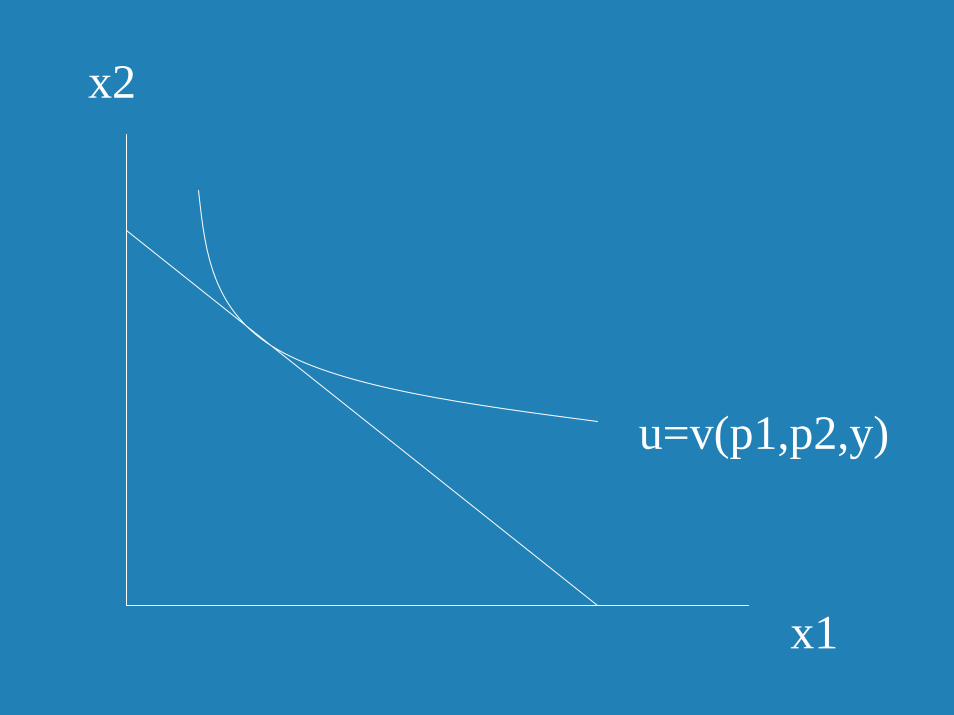
•• v(v(pp, y)= u(, y)= u(x(px(p,y)),y))•• When u is continuous, x exist, When u is continuous, x exist,

then v is wellthen v is well--defined.defined.•• From graph, v(p,y) gives the From graph, v(p,y) gives the

value of utility of the highest value of utility of the highest indifference curve that is indifference curve that is tangent to the budget line.tangent to the budget line.

u=v(p1,p2,y)

x1

x2

mf620 1/2007 5

1.4.1 Indirect Utility 1.4.1 Indirect Utility Function: PropertiesFunction: Properties

•• 1. Continuous at all p, y >01. Continuous at all p, y >0•• 2. Homogenous of degree zero in 2. Homogenous of degree zero in

(p, y)(p, y)•• 3. Strictly increasing in y3. Strictly increasing in y•• 4. Decreasing in prices4. Decreasing in prices•• 5. Quasiconvex in (p, y)5. Quasiconvex in (p, y)

mf620 1/2007 6

1.4.1 Indirect Utility 1.4.1 Indirect Utility Function: PropertiesFunction: Properties•• 6. Roy6. Roy’’s Identity:s Identity:

–– xx11 (p, y) = (p, y) = -- ∂∂v/v/∂∂pp11 / / ∂∂v/v/∂∂yyProofProof1.1. By the theorem of the MaximumBy the theorem of the Maximum2.2. To show that v(To show that v(tptp,,tyty)=t)=t00v(p,y). v(p,y).

Intuitively, the budget line is not Intuitively, the budget line is not shifted.shifted.

3. 3. ∂∂v/v/∂∂y > 0. Using the envelop theorem, y > 0. Using the envelop theorem, we know this is equal to we know this is equal to λλ* * and > 0 .and > 0 .

Intuitively, more income leads to higher Intuitively, more income leads to higher utility.utility.

mf620 1/2007 7

1.4.1 Indirect Utility 1.4.1 Indirect Utility Function: PropertiesFunction: Properties

4. 4. ∂∂v/v/∂∂p < 0. Use envelope p < 0. Use envelope theorem.theorem.

5. By definition5. By definitionv(pv(ptt,,yytt) ) ≤≤ max[v(pmax[v(p11,y,y11 ), v(p), v(p22,y,y22 )])]Consumers prefers one of any two Consumers prefers one of any two

extreme budget sets to any extreme budget sets to any average of the two.average of the two.

mf620 1/2007 8

1.4.1 Indirect Utility 1.4.1 Indirect Utility Function: PropertiesFunction: Properties

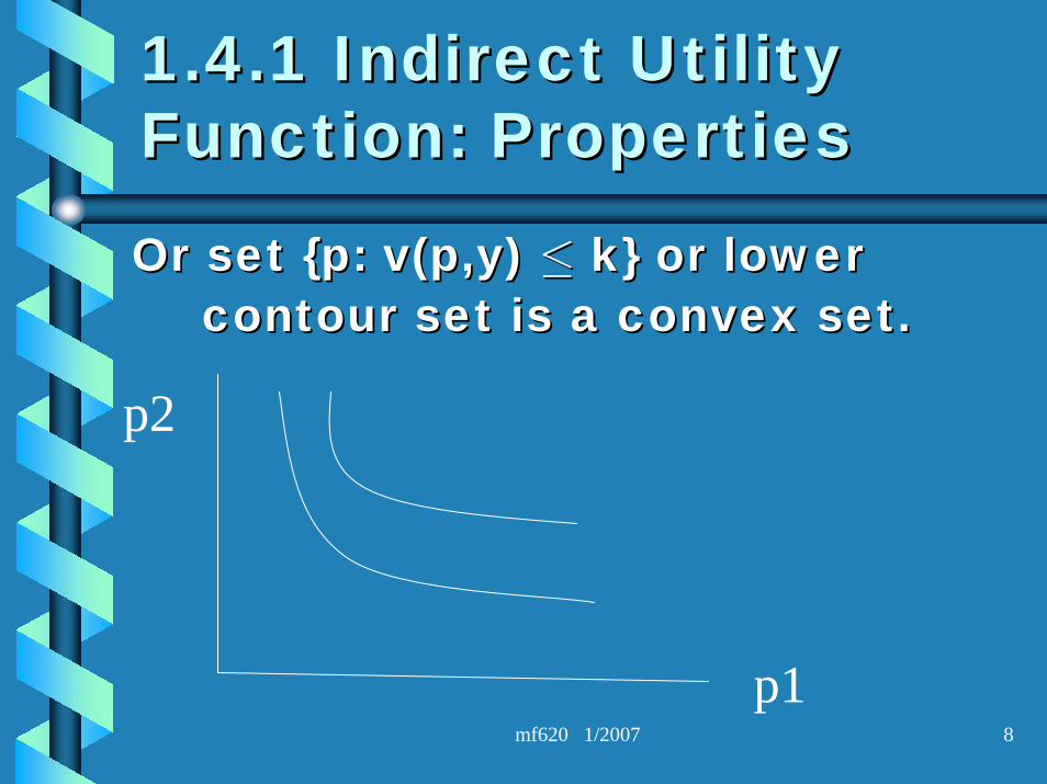
Or set {p: v(p,y) Or set {p: v(p,y) ≤≤ k} or lower k} or lower contour set is a convex set.contour set is a convex set.

p1

p2

mf620 1/2007 9

1.4.1 Indirect Utility 1.4.1 Indirect Utility Function: PropertiesFunction: Properties

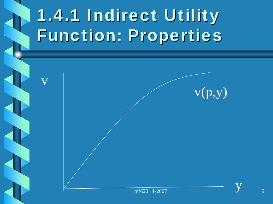
y

vv(p,y)

mf620 1/2007 10

1.4.1 Indirect Utility 1.4.1 Indirect Utility Function: PropertiesFunction: Properties

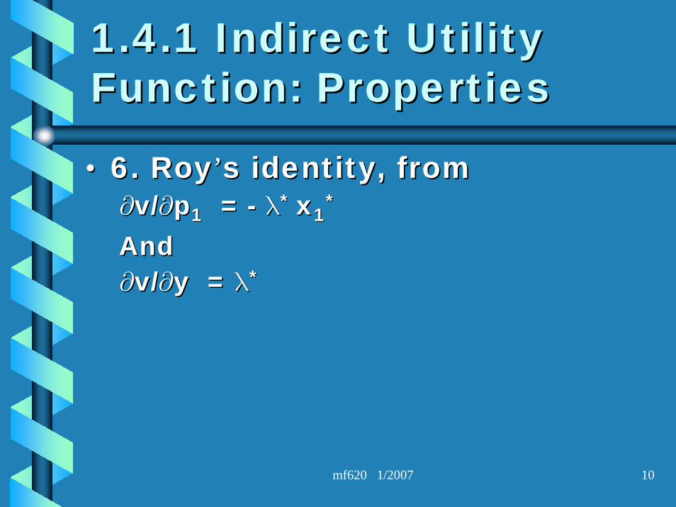
•• 6. Roy6. Roy’’s identity, froms identity, from∂∂v/v/∂∂pp11 = = -- λλ* * xx11

**

And And ∂∂v/v/∂∂y = y = λλ* *

mf620 1/2007 11

1.4.1 Indirect Utility 1.4.1 Indirect Utility Function: PropertiesFunction: Properties

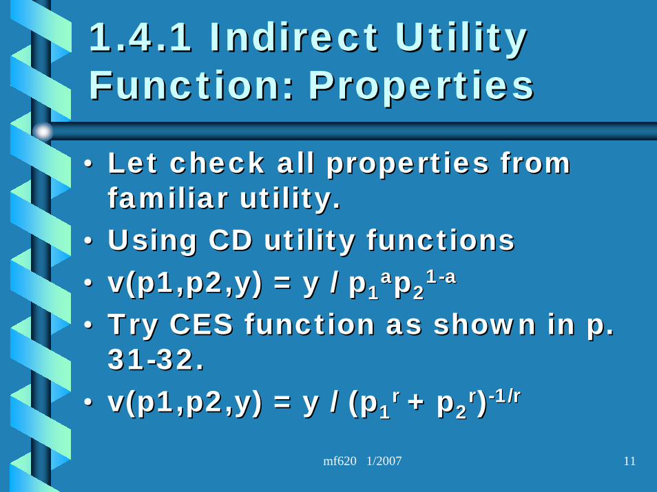
•• Let check all properties from Let check all properties from familiar utility.familiar utility.

•• Using CD utility functionsUsing CD utility functions•• v(p1,p2,y) = y / v(p1,p2,y) = y / pp11

aapp2211--aa

•• Try CES function as shown in p. Try CES function as shown in p. 3131--32.32.

•• v(p1,p2,y) = y / (v(p1,p2,y) = y / (pp11r r + p+ p22

rr))--1/r1/r

mf620 1/2007 12

1.4.2 Expenditure 1.4.2 Expenditure FunctionFunction

•• What is the minimum level of What is the minimum level of money or expenditure needed money or expenditure needed for given prices to get a given for given prices to get a given level of utility?level of utility?

•• minminxx px stpx st. u(x) . u(x) ≥≥ u.u.•• We specify the attainable level We specify the attainable level

of u, then ask for the minimum of u, then ask for the minimum money of achieving it.money of achieving it.

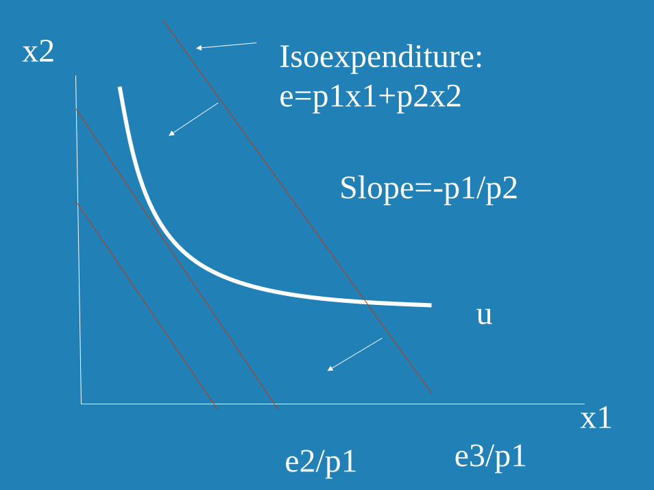
x1

x2

u

Slope=-p1/p2

e2/p1 e3/p1

Isoexpenditure: e=p1x1+p2x2

mf620 1/2007 14

1.4.2 Expenditure 1.4.2 Expenditure FunctionFunction

•• minminxx px stpx st. u(x) . u(x) ≥≥ u. u. •• Let Let xxhh(p,u) solves the problem(p,u) solves the problem•• The lowest expenditure to get u The lowest expenditure to get u

is equal to is equal to pxpxhh(p,u) (p,u) •• Let e(p,u) Let e(p,u) ≡≡ pxpxhh(p,u) (p,u) •• Called the Expenditure function.Called the Expenditure function.

mf620 1/2007 15

1.4.2 Expenditure 1.4.2 Expenditure FunctionFunction

•• xxhh(p,u) is called Hicksian (p,u) is called Hicksian Demand or Compensated Demand or Compensated demand function.demand function.

•• We can draw the Hicksian We can draw the Hicksian demand for good1 by letting the demand for good1 by letting the price of x1 to vary, as we did for price of x1 to vary, as we did for the Marshallian demand. the Marshallian demand.

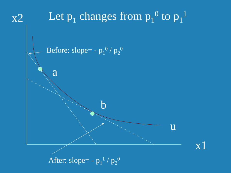
x1

x2 Let p1 changes from p10 to p1

1

Before: slope= - p10 / p2

0

After: slope= - p11 / p2

0

a

b

u

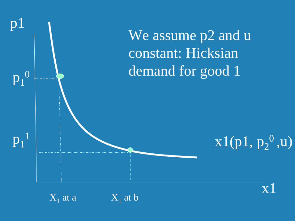
x1

p1

x1(p1, p20 ,u)

p10

p11

X1 at a X1 at b

We assume p2 and u constant: Hicksian demand for good 1

mf620 1/2007 18

1.4.2 Expenditure 1.4.2 Expenditure FunctionFunction•• Hicksian demand tells us what Hicksian demand tells us what

consumption bundles achieves a consumption bundles achieves a targeted utility and minimizes total targeted utility and minimizes total expenditure.expenditure.

•• Compensated term means Compensated term means ““as price of as price of good 1 varies (goes up), you lose some good 1 varies (goes up), you lose some utility, so to keep u constant, you utility, so to keep u constant, you needed to be compensated to be as needed to be compensated to be as happy as before.happy as before.

•• Hicksian demand is not directly Hicksian demand is not directly observable since it depends on utility, observable since it depends on utility, which is not observable.which is not observable.

mf620 1/2007 19

1.4.2 Expenditure 1.4.2 Expenditure Function: propertiesFunction: properties

•• Theorem 1.7Theorem 1.7•• 1. Continuous in p1. Continuous in p•• 2. Strictly increasing in u2. Strictly increasing in u•• 3. Increasing in p3. Increasing in p•• 4. Homogenous of degree 1 in p4. Homogenous of degree 1 in p•• 5. Concave in p5. Concave in p

mf620 1/2007 20

1.4.2 Expenditure 1.4.2 Expenditure Function: propertiesFunction: properties

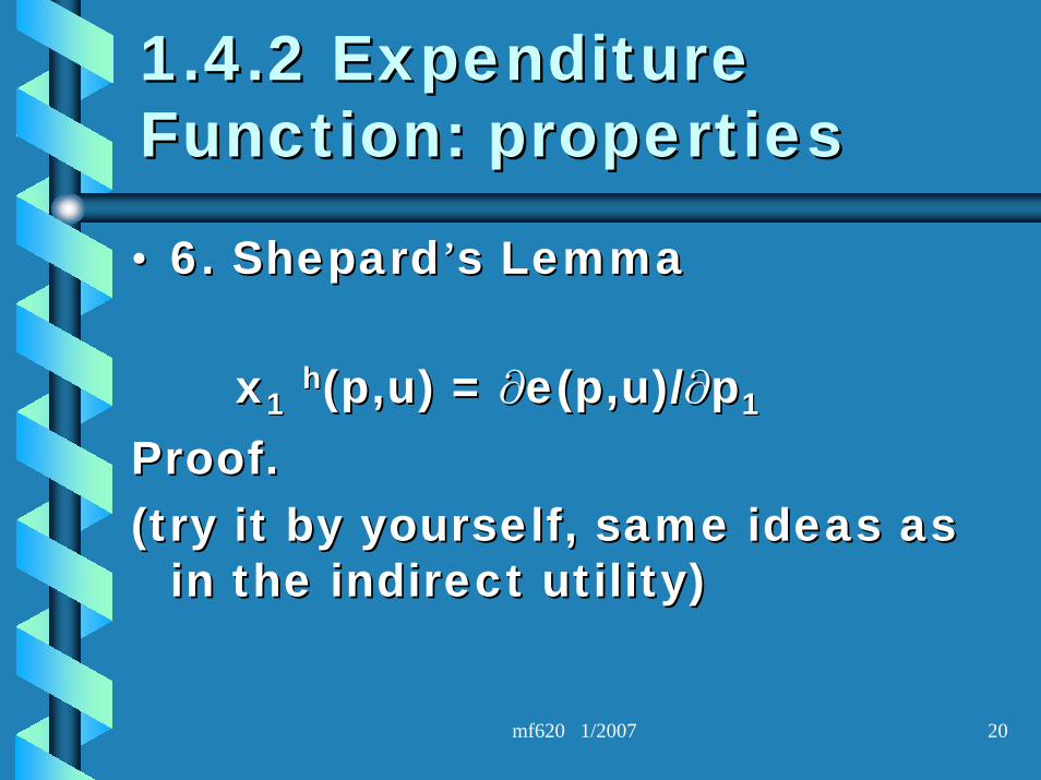
•• 6. Shepard6. Shepard’’s Lemmas Lemma

xx11hh(p,u) = (p,u) = ∂∂e(p,u)/e(p,u)/∂∂pp11

Proof.Proof.(try it by yourself, same ideas as (try it by yourself, same ideas as

in the indirect utility)in the indirect utility)

mf620 1/2007 21

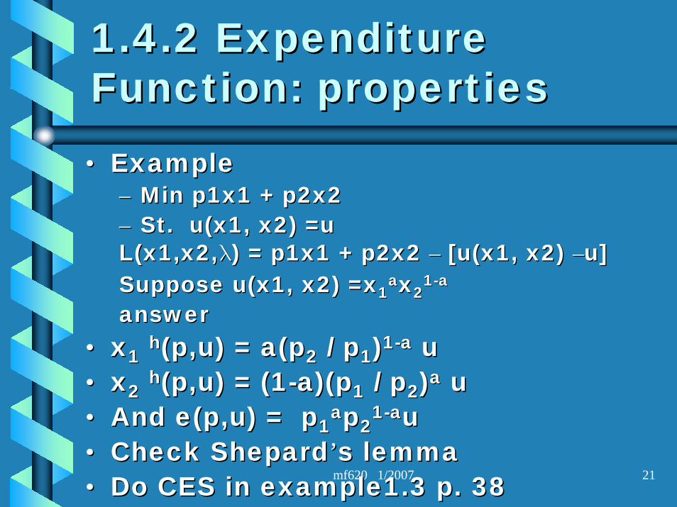
1.4.2 Expenditure 1.4.2 Expenditure Function: propertiesFunction: properties•• ExampleExample

–– Min p1x1 + p2x2Min p1x1 + p2x2–– St. u(x1, x2) =uSt. u(x1, x2) =uL(x1,x2,L(x1,x2,λλ) = ) = p1x1 + p2x2 p1x1 + p2x2 –– [u(x1, x2) [u(x1, x2) ––u]u]Suppose u(x1, x2) =xSuppose u(x1, x2) =x11

aaxx2211--aa

answeranswer•• xx11

hh(p,u) = a(p(p,u) = a(p22 / p/ p11))11--aa uu•• xx22

hh(p,u) = (1(p,u) = (1--a)(pa)(p11 / p/ p22))aa uu•• And e(p,u) = pAnd e(p,u) = p11

aapp2211--aauu

•• Check ShepardCheck Shepard’’s lemmas lemma•• Do CES in example1.3 p. 38Do CES in example1.3 p. 38

mf620 1/2007 22

1.4.3 Relations between 1.4.3 Relations between Expenditure and Indirect utilityExpenditure and Indirect utility

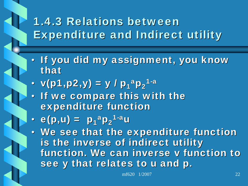
•• If you did my assignment, you know If you did my assignment, you know that that

•• v(p1,p2,y) = y / v(p1,p2,y) = y / pp11aapp22

11--aa

•• If we compare this with the If we compare this with the expenditure function expenditure function

•• e(p,u) = pe(p,u) = p11aapp22

11--aauu•• We see that the expenditure function We see that the expenditure function

is the inverse of indirect utility is the inverse of indirect utility function. We can inverse v function to function. We can inverse v function to see y that relates to u and p.see y that relates to u and p.

mf620 1/2007 23

Theorem 1.8 Duality between Theorem 1.8 Duality between indirect utility and expenditureindirect utility and expenditure

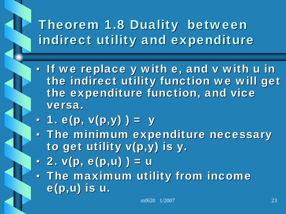
•• If we replace y with e, and v with u in If we replace y with e, and v with u in the indirect utility function we will get the indirect utility function we will get the expenditure function, and vice the expenditure function, and vice versa.versa.

•• 1. e(p, v(p,y) ) = y 1. e(p, v(p,y) ) = y •• The minimum expenditure necessary The minimum expenditure necessary

to get utility v(p,y) is y.to get utility v(p,y) is y.•• 2. v(p, e(p,u) ) = u2. v(p, e(p,u) ) = u•• The maximum utility from income The maximum utility from income

e(p,u) is u.e(p,u) is u.

mf620 1/2007 24

Theorem 1.8 Duality between Theorem 1.8 Duality between indirect utility and expenditureindirect utility and expenditure

•• This duality lets us work with one This duality lets us work with one problem and invert them to get problem and invert them to get solution of another problem.solution of another problem.

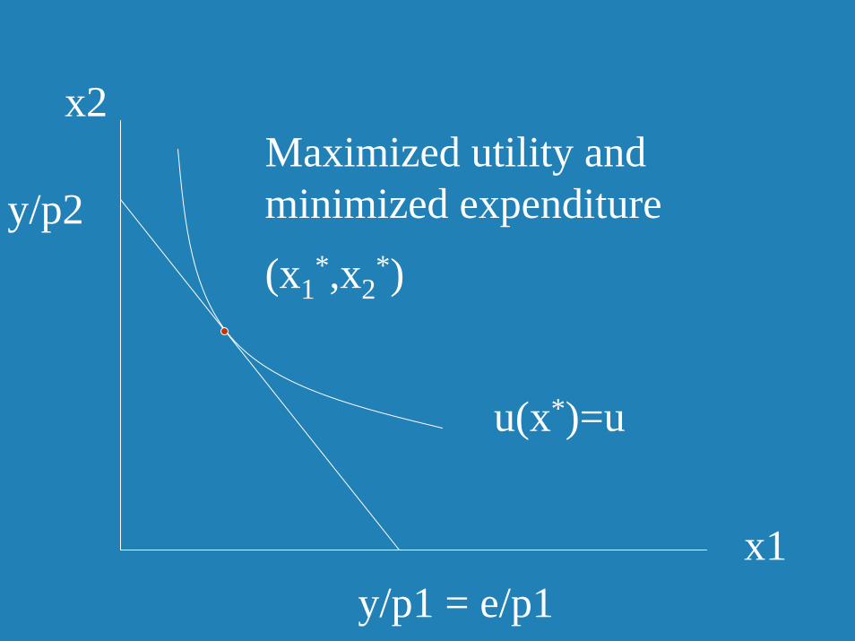
x2

x1

u(x*)=u

y/p1 = e/p1

y/p2(x1

*,x2*)

Maximized utility and minimized expenditure

mf620 1/2007 26

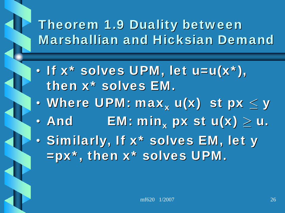
Theorem 1.9 Duality between Theorem 1.9 Duality between Marshallian and Hicksian DemandMarshallian and Hicksian Demand

•• If x* solves UPM, let u=u(x*), If x* solves UPM, let u=u(x*), then x* solves EM.then x* solves EM.

•• Where UPM: Where UPM: maxmaxxx u(x) u(x) st pxst px ≤≤ yy•• And EM: minAnd EM: minxx px stpx st u(x) u(x) ≥≥ u.u.•• Similarly, If x* solves EM, let y Similarly, If x* solves EM, let y

==pxpx*, then x* solves UPM.*, then x* solves UPM.

mf620 1/2007 27

Theorem 1.9 Duality between Theorem 1.9 Duality between Marshallian and Hicksian DemandMarshallian and Hicksian Demand

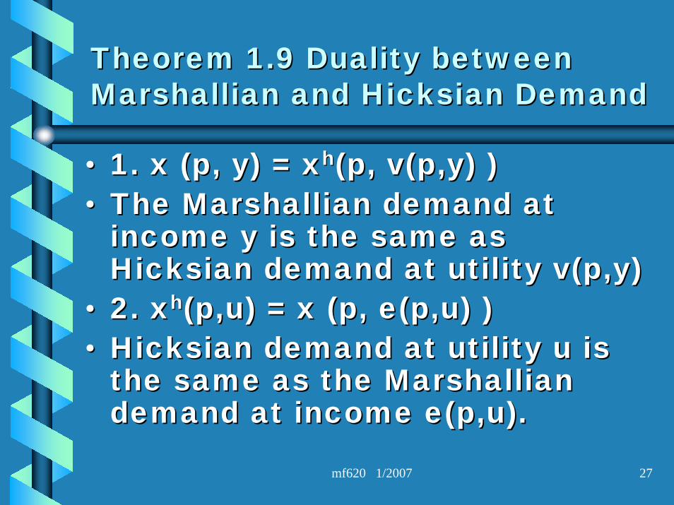
•• 1. x (p, y) = 1. x (p, y) = xxhh(p, v(p,y) )(p, v(p,y) )•• The Marshallian demand at The Marshallian demand at

income y is the same as income y is the same as Hicksian demand at utility v(p,y)Hicksian demand at utility v(p,y)

•• 2. 2. xxhh(p,u) = x (p, e(p,u) )(p,u) = x (p, e(p,u) )•• Hicksian demand at utility u is Hicksian demand at utility u is

the same as the Marshallian the same as the Marshallian demand at income e(p,u).demand at income e(p,u).

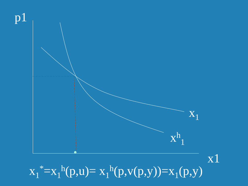
p1

x1

xh1

x1

x1*=x1

h(p,u)= x1h(p,v(p,y))=x1(p,y)

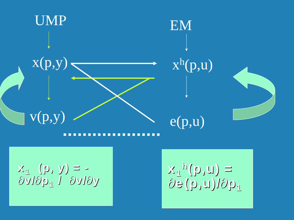
UMP

x(p,y)

v(p,y)

EM

xh(p,u)

e(p,u)

xx11hh(p,u) = (p,u) =

∂∂e(p,u)/e(p,u)/∂∂pp11

xx11 (p, y) = (p, y) = --∂∂v/v/∂∂pp11 / / ∂∂v/v/∂∂yy