EC422 Mathematical Economics 2 - econ.tu.ac.th

Chaiyuth Punyasavatust 1

EC422 Mathematical Economics 2

Chaiyuth Punyasavatsut


Course materials and evaluation• Texts: Dixit, A.K ; Sydsaeter et al.• Grading: 40,30,30. OK or not.• Resources:

ftp://econ.tu.ac.th/class/archan/CHAIYUTH/




Objectives

• Dynamic economics is about explaining economic behaviors through time.

• Explain the time paths of economic variables.

• Optimization concept.• The choice is the use of resources in

different time periods.• Maximizing a multiperiod objective

function of variables in many periods, subject to budget or resource constraints on these variables through time.


Objectives

• Find optimal time path for every choice variable.

• Three major approaches: Calculation of variation, maximum principle or optimal control theory (Hamiltonian), and dynamic programming (Bellman equation).

• And also method of Lagrange


Example: Economic Growth• choice between current consumption

and future consumption. • By reducing consumption today, will

lead to more resources or capital stock that can be used to produce consumption goods for future.

• What is the optimum consumption decision in each period.


Example: Business Cycles• Market equilibrium in a dynamic

setting• Explaining economic fluctuations

from technology shocks


Example: Dynamic Games• Oligopoly pricing• Two players try to solve the standard

optimization problem where the state variable depends on control variables chosen by both players.

• Nash equilibrium vs subgame perfect• Stackelberg game


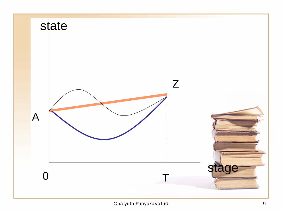
Common ingredients• 1. Initial point and terminal point• 2. Admissible paths from initial to terminal• 3. Path values• 4. Objective to max or min path value

and get the optimal path.


state

stageT0

Z

A


Mathematics is a language.

Lecture 1 Preliminary Mathematics


Convex Sets• 1. We often assume this or convexity

to guarantee that our analysis is tractable mathematically and the results are well-behaved or clear-cut.

• 2. A set is convex if for any two points in the set, all convex combinations of those two points are also points in the same set.


Convex Sets

“ S is a convex set if for all x1 and x2

belong to S, we havet x1 + (1--t) x2 ∈ S, for all t ∈ 0 ≤ t ≤ 1.”

• Equivalently, a set is convex iff we can connect any two points in the set by a straight line that lie entirely within this set.

• 3. For example, consider two points in a real line, R.


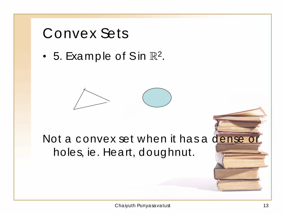
Convex Sets• 5. Example of S in R2.

Not a convex set when it has a dense or holes, ie. Heart, doughnut.


Closed Sets

• 1. Consider the simplest case, a close interval, [a, b], in the real line is a closed set. The sets on both sides of this interval (open interval) are open sets. The union of open sets is an open set. Thus, [a, b]c is an open set.


Closed Sets• 2. We call [a, b] a closed

set if its complement is an open set.

• 3. A set is closed if it contains all of the points in its boundary.


Bounded Sets• 1. Every open interval on

the real line, (a, b) ⊂ R is a bounded set.

• 2. In R2, an open ball is a disk containing set of points inside (excluding the circumference).

• 3. In R3, an open ball is the set of points inside the sphere of radius ε.


Compact Sets• 1. A set S in Rn is called

compact if it is closed and bounded.

• 2. Any open interval in R is not a compact set. (since not closed)

• 3. An open ball in Rn is not compact, similarly.

• 4 Rn is not compact since it is not bounded.


Real-valued functions

f is a real-value function if it maps elements of its domain into the real line.

Ex. Y = ax1 + bx2Ex. U = x1*x2


Level set• This allows us to study functions

of three variables by looking upon sets in the two dimensional plane.

• 1. A level set is the set of all elements in the domain of a function that map into the same number in the range.


Level set• 2. L( y=10) is a level set of the

real-valued function f : D → Riff L( y=10) = {x | x ∈ D, f(x) =10 }.

Ex. An isoquant is a set that all input bundles producing exactly 10 units of output.

• 3. Note that since f is a function-- that is it assigns a single number in the range—therefore, two difference level sets will never cross each other.


Level Set• Draw a picture


Level set• 4. Draw level sets in R2 and define

the superior set, S(y=10)≡ {x| x∈ D, f(x) ≥ 10}, for level y=10.

Ex. An input requirement set is a se of all input bundles that produce at least y units of output.

• 5. When f(x) is increasing, then S(y=10) will always lie on and above the level set L(y=10)


Level set• 6. Note that (a) f is increasing if f(x0)

≥ f(x1), for all x0 ≥ x1. (notice vector notation here).

• 7. Think of the level sets when f is decreasing.


Concave functions.• 1. In economics, we often see concave

real-valued functions when domains are convex sets.

• 2. f is a concave function iff for every pair of points on its graph, the chord joining them lies on or below the graph. Here, we look at the value of the function evaluated at convex combinations of any two points.


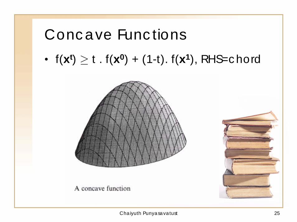
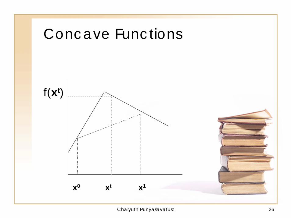
Concave Functions• f(xt) ≥ t . f(x0) + (1-t). f(x1), RHS=chord


Concave Functions

f(xt)

x0 xt x1


Concave functions.• 3. Another equivalent definition: f is a

concave function iff the set of points on and below (i.e. beneath) the graph is a convex set.

• 4. A concave function allows for linear segments. To rule out this, we require a strictly concave function.

• 5. “Strictly” normally is equivalent to get rid of equality sign in definition.


Concave functions.• 6. So, f is a strictly concave function

iff the chords joining any pairs of points must lie below the graph.

• 7. Nice properties of the concave functions are (1) the critical points are alwaysmaxima; (2) sum of concave functions is concave;


Concave functions.• (3) their level sets have just the right

shapes; they bound convex subsets from below.

• For (2), we need it for the grand utility or social welfare function.

• For (3), it has nice interpretations, diminishing marginal rate of substitution, and mixing goods make you happier.


Concave functions.• 8. A monotonic transformation of a

concave function needs not be concave.

• In fact, any monotonic transformation of a concave function is a quasiconcave function. Think of f(x) = x, and g(x) = x2.


• g is a monotonic transformation of I if g is strictly increasing function of I.

• Example. U(x,y)= xy. • Then, 3xy+2, (xy) 2, (xy) 2 +2, ln

(xy) are its monotone transformation.

• We use this property for an ordinal concept of utility.


Quasiconcave functions• 1. f is a quasiconcave function iff

the superior set is a convex set.• 2. The superior set is the set

containing points in domain that gives the function a value ≥ a specific value of y. So, it is the area on and above the level set of a given value of y.


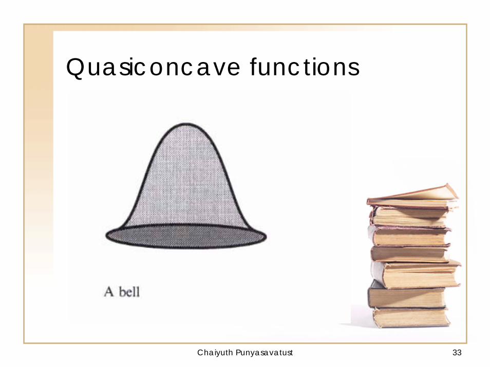
Quasiconcave functions


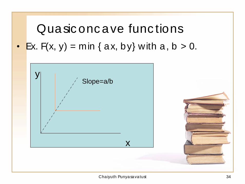
Quasiconcave functions• Ex. F(x, y) = min { ax, by} with a, b > 0.

y

x

Slope=a/b


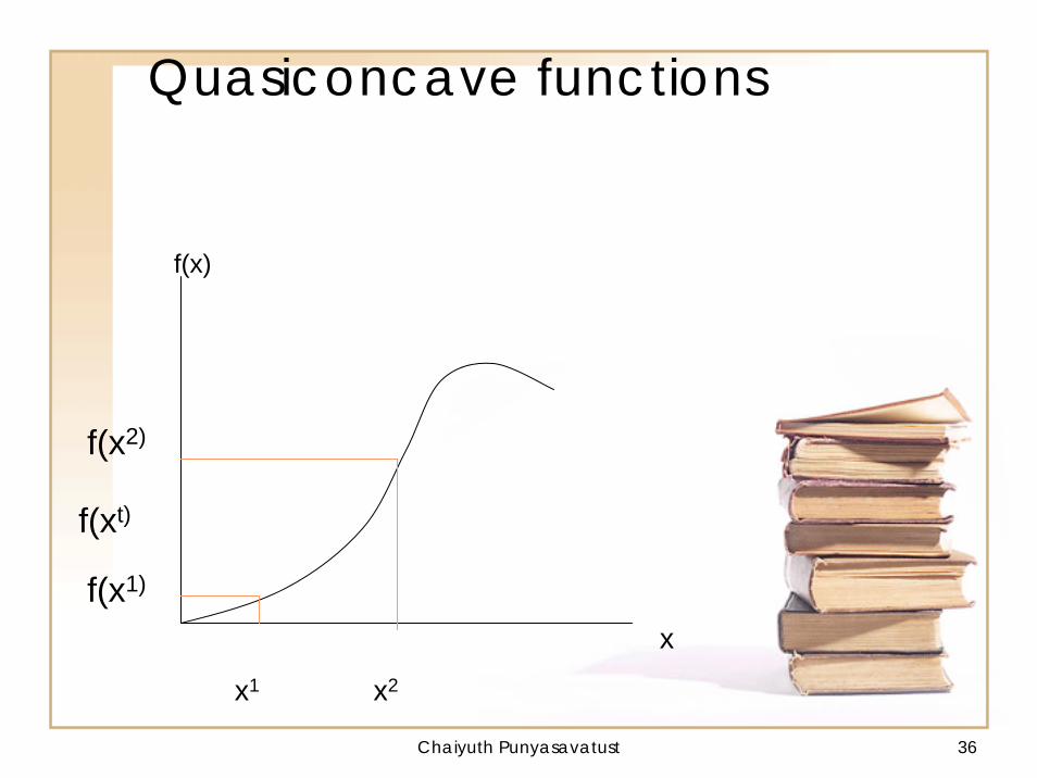
Quasiconcave functions• 3. Another definition is to look at the value of

the function: the value of the function at points formed by convex combination must be greater or equal the lowest value of the functions at any two points.

• That is, if f(x1) < f(x2), then f(x t) ≥ f(x1), for all t between 0 and 1, and x t ≡ t x1 + (1-t)x2.

• f(x t) ≥ Min [ f(x1), f(x2) ], for all t ∈[0,1]. Read “the smaller of ..”



f(x)

x

x1 x2

f(xt)

f(x1)

f(x2)



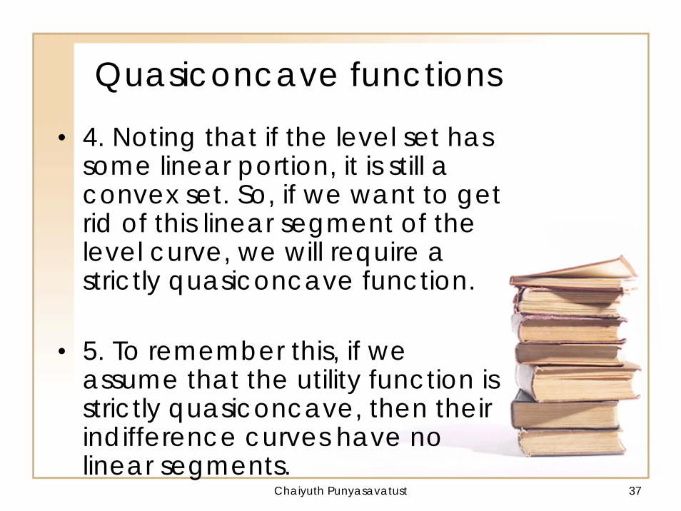
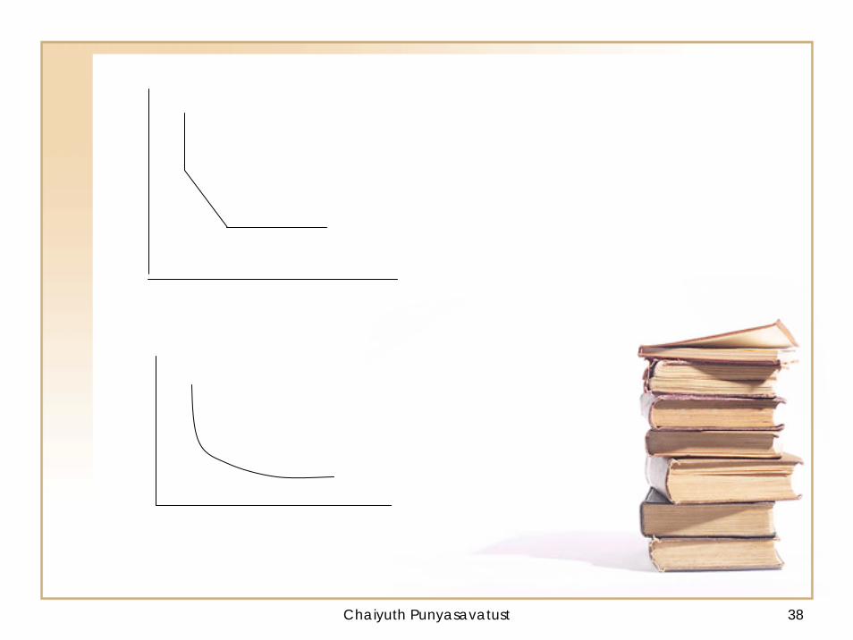
• 4. Noting that if the level set has some linear portion, it is still a convex set. So, if we want to get rid of this linear segment of the level curve, we will require a strictly quasiconcave function.

• 5. To remember this, if we assume that the utility function is strictly quasiconcave, then their indifference curves have no linear segments.



Quasiconcave functions• 6. Some properties of quasiconcave

functions: • (1) sum of quasiconcave functions is

not necessary quasiconcave; • (2) a critical point need not be a

maximum. For (1), think of z=x3-x, we know that both x3 and –x are both monotone in R, so they are quasiconcave, but z, a sum of quasiconcave functions is neither quasiconcave nor quasiconvex.


Concavity and quasiconcavity• 1. A concave function is always

quasiconcave. So, does the strictly function.

• 2. The reverse is not true. I.e. the bell curve, graph of x3 , a step function

• 3. From (1), we know that superior sets of a quasiconcave function are convex.

• 4. The linear graph is both quasiconcave and quasiconvex.


Concavity and quasiconcavity• 5. So far, we should feel that

we only need a function to be only a quasiconcave, if we need only a nice level curve that is convex to the origin, and a strictly quasiconcave for a nicer level curve.


Checking Concavity• 1. R1 : f is concave iff f " ≤ 0, for all x.2. R2 : f is concave iff the Hessian matrix is

negative semidefinite for all x in domain. The simplest way to check this is to verify that for all x, f11 ≤ 0 and f22 ≤ 0. Note that f11 is just a change in slope of the function in the direction of x1, keeping x2 constant. And for f12 is just a curvature of the function when x1 and x2 change at the same time. This rule of thumb does not allow for both zero values of f11 and f22.


Checking Concavity2.1 The precise way to check for a

concave function for two variables is to verify that (a) f11 ≤ 0; and (b) f11 f22 - f12f21 ≥ 0.

2.2 Conditions (a) and (b) are equivalently stated as the principal minors of the Hessian matrix always alternate in sign, starting with negative.

2.3 Principal minors are just the determinants of submatrices evaluated at the point x, as we move down the principal diagonal of the Hessian.


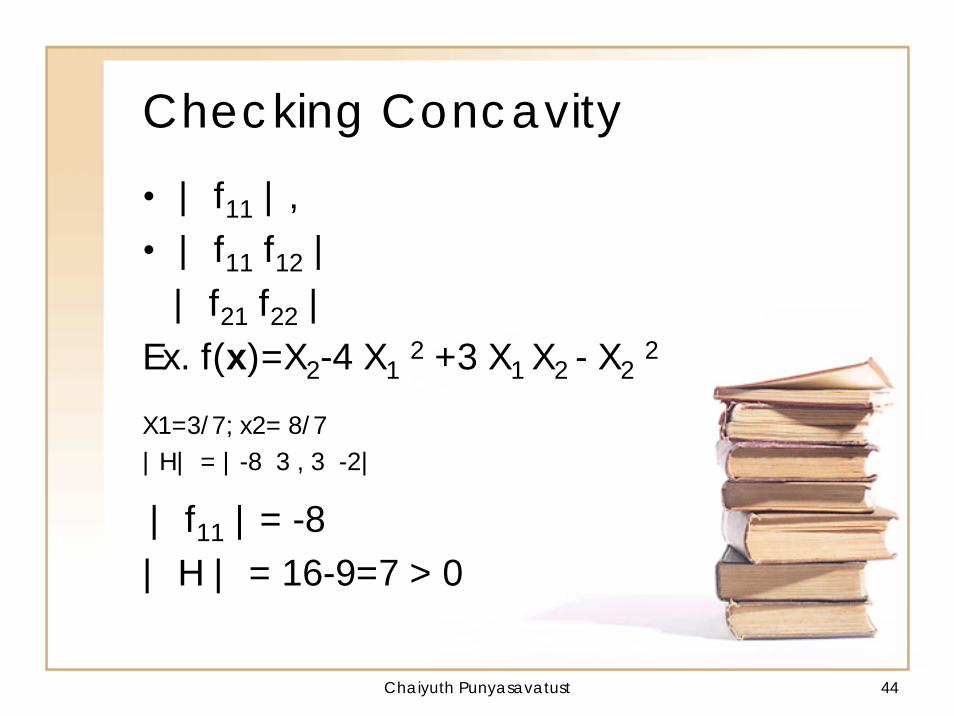
• | f11 |, • | f11 f12 |

| f21 f22 |Ex. f(x)=X2-4 X1

2 +3 X1 X2 - X22

X1=3/7; x2= 8/7|H| = |-8 3 , 3 -2|

| f11 |= -8| H | = 16-9=7 > 0

Checking Concavity


Checking Concavity

• 3. So, the Hessian matrix tells us about the curvature of the function evaluated at certain points.

• 4. For a strictly concave function, we require the Hessian matrix to be negative definite for all x in domain set. That is, we need f11 < 0 and f22< 0.


• 5. Example: f(x1, x2 )= x10.5x2

0.5. We can verify that f11 ≤ 0 and f22 ≤ 0 for all x in domain. Thus, f is a concave function, and is also quasiconcave.

• 6. How about f(x1, x2 ) = x1x2 . Here we have f11 = 0 and f22 = 0 and the determinant of the Hessian matrix (second order principal minor) is 0. In fact, this function is not neither concave nor convex.

Checking Concavity


Homogenous functions• 1. f is homogenous of degree k

if f(tx) = tk f(x), for all t > 0.• 2. When k =1, f is also called

linear homogenous.• 3. f(x) = A is homogenous

of degree . This function is also known as Cobb-Douglas function.

• 4. If f is homogenous of degree k, its partial derivatives are homogenous of degree k-1.

x x1 2α β

α β+


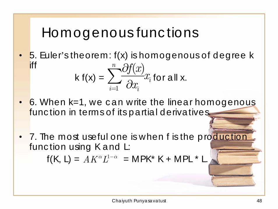
Homogenous functions• 5. Euler’s theorem: f(x) is homogenous of degree k

iffk f(x) = for all x.

• 6. When k=1, we can write the linear homogenous function in terms of its partial derivatives.

• 7. The most useful one is when f is the production function using K and L:

f(K, L) = = MPK* K + MPL * L.

n

ii i

f x xx1

( )=

∂∂∑

AK L1α α−


Useful theorems• 1. If f is quasiconcave and linearly

homogenous, then f is concave.• 2. Every Cobb-Douglas function of

two variables is quasiconcave.• 3. CES function is quasiconcave since

it is a monotonic transformation of a concave function.

• 4. A Cobb-Douglas function is concave iff it is CRTS or DRTS.


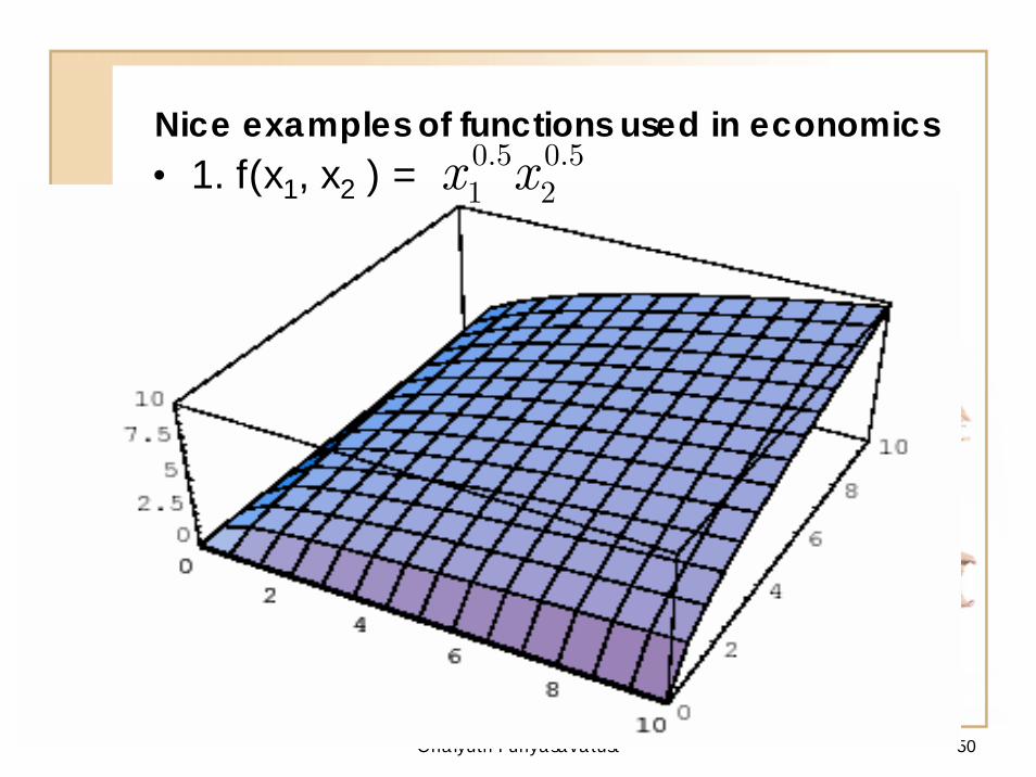
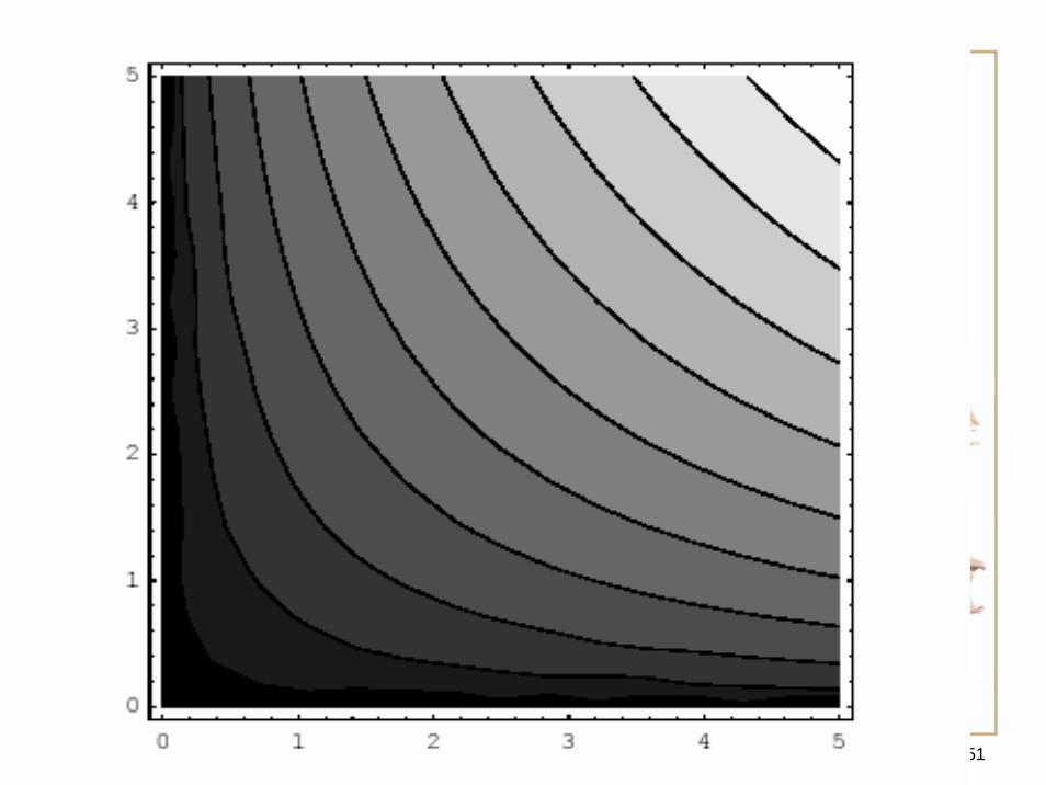
Nice examples of functions used in economics• 1. f(x1, x2 ) = x x0.5 0.5

1 2



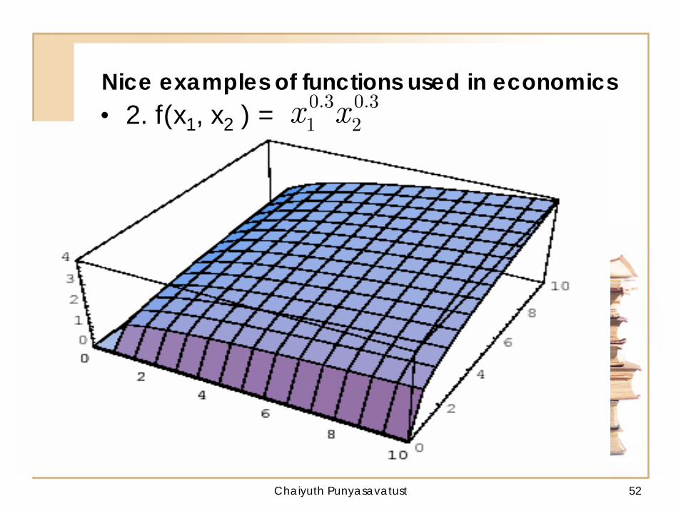
Nice examples of functions used in economics• 2. f(x1, x2 ) = x x0.3 0.3

1 2


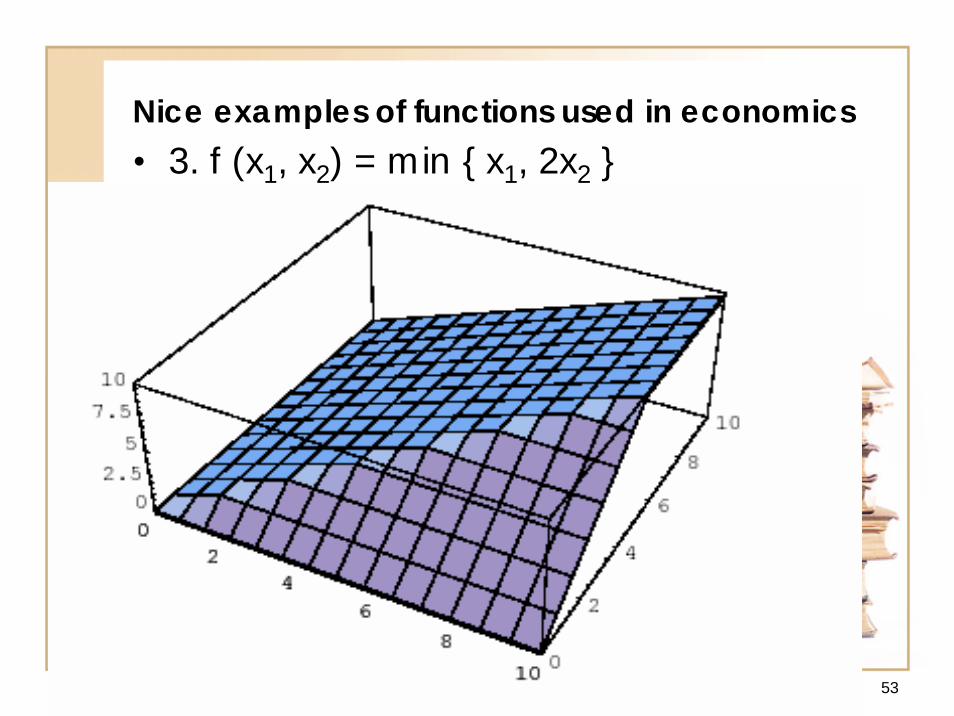
Nice examples of functions used in economics• 3. f (x1, x2) = min { x1, 2x2 }


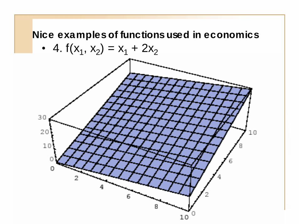
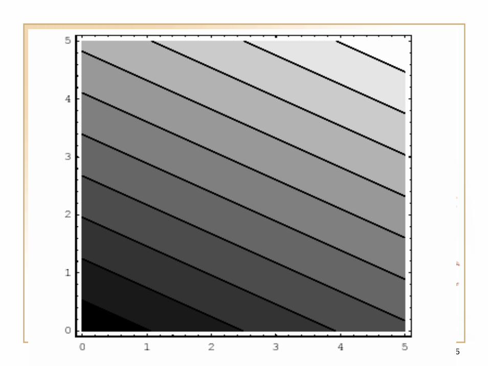
Nice examples of functions used in economics• 4. f(x1, x2) = x1 + 2x2


Documents

EC422 Mathematical Economics 2 - econ.tu.ac.th